Embed Size (px)
Citation preview
IMPACT OF FINANACIAL DERIVATIVES ON STOCK MARKET
VOLATILITY IN INDIA
Management Research Project -II
Submitted In the partial fulfillment of the Degree of Master of Business Administration
Semester-IV
By
Devanshi Barbhaya (12044311001)
Kinjal Bhadani (12044311003)
Nikshubha Goswami (12044311031)
Hetal Mistri (12044311048)
Arpita Patel (12044311068)
Under the Guidance of:
Prof. (Dr.) Mahendra Sharma Prof. & Head,
V. M. Patel Institute of Management.
&
Jayesh D. Patel Assistant Professor,
V. M. Patel Institute of Management.
Submitted To: V. M. Patel Institute of Management
(April 15, 2014)
i
CERTIFICATE BY THE GUIDE
This is to certify that the contents of this report entitled “Impact of financial derivative on
stock market volatility” submitted to V. M. Patel Institute of Management for the Award of
Master of Business Administration (MBA Sem-IV) is original research work carried out by
him/her/them under my supervision. This report has not been submitted either partly or
fully to any other University or Institute for award of any degree or diploma.
Name Exam number
Devanshi barbhaya (12044311001)
Kinjal bhadani (12044311003)
Nikshubha goswami (12044311031.)
Hetal mistri (12044311048.)
Arpita patel (12044311068)
Professor & Head,
V. M. Patel Institute Of Management,
Ganpat University.
Kherva.
Date :
Place :

ii
CANDIDATE’S STATEMENT
We hereby declare that the work incorporated in this report entitled “_The volatity
derivative of future price_” in partial fulfillment of the requirements for the award of
Master of Business Administration (Sem.-IV) is the outcome of original study undertaken
by us and it has not been submitted earlier to any other University or Institution for the
award of any Degree or Diploma.
Devanshi barbhay (12044311001)
Kinjal bhadani (12044311003)
Nikshubha goswami (12044311031)
Hetal mistri (12044311048)
Arpita patel (12044311068)
Date:
Place:

iii
PREFACE
One can deny for the importance of the practical exposure of the problem for its better
understanding and better grip of coming out with an industrially acceptable solution.
Being the Management student and performing small practical even is in itself an experience of
responsibility on our head. The project is certainly the best chance to work in the Management field
and have practical understanding of Management Strategic Planning and his implementation. This
exposure has really added a supplement and nourishment to our growing tree of management
knowledge- just like the fertilizer does to the plants.
In view of above, this report has been completed as a part of syllabus prescribed for the master of
business administration. This had been made in order to know volatility derivative of future price in
stock market overview and its strategic tools and its planning.
Barbhaya Devanshi 12044311001
Bhadani Kinjal 12044311003
Goswami Nikshubha 12044311031
Mistri Hetal 12044311040
Patel Arpita 12044311068

iv
ACKNOWLEDGEMENT
It is indeed of great moment to pleasure to express our sense of per found gratitude and ineptness
to all the people who have been instrumental in making our learning a rich experience. We got the
opportunity to do a challenging project in Management Research Project. The project is the
important part of our study and gives us a practical exposure to financial Tools its implementation
and it is almost impossible to do the same without the guidance of people in and around us.
It gives me immense pleasure to acknowledge financial Tools which has been nice enough to give
our chance to do our Report and providing us support throughout our Report period and
afterward.
We hereby take the pleasure of thanking all who have contributed to the making of this report.
Firstly we would like to thank Mr. Abhishek Parikh and Mr. Jayesh Patel , Who has provided
us full liberty, co –operation during our Report and sharing knowledge of her field with us always
with a smile.
THANK YOU.
v
CONTENTS
No. Name Page No.
Certificate by the Guide i
Candidate’s Statement ii
Preface iii
Acknowledgments Iv
List of Tables xiii
1 Introduction 1
1.2 Applications of Financial Derivatives 4
1.3 Volatility can be categorized as 10
1.4 Real economic effects of financial market volatility 11
1.5 Causes of Volatility 12
1.6 Measures to control volatility: 16
1.7 Measuring Volatility 19
1.8 Motivation of the Study 24
1.9 Reference 25
2 Review of literature 26
2.1 Reference 31
3 Research methodology 33
3.1 Statement of the problem 33
3.2 Objectives of the study 34
3.3 Hypotheses of the Study 34
3.4 Research design 34
3.5 Software’s used 36
3.7 Limitations of the Study 39
4 Impact of index futures on expected price 40
4.1 Impact of index futures on price discovery 40
4.1.1 The ARCH Model 41
4.1.2 The GARCH Model 41
4.1.3 Independent samples t- Test 42

vi
4.2 Implication of the study 45
5 Findings 47
6 Conclusion 48
7 Reference and Bibliography 49
8
Appendices 51

vii
LIST OF TABLES
NO. Name Page No.
1.1 Market timings of various products / markets in India 17
4.1 Group Statistics 44
4.2 Levine statistics for equality of variances 44
4.3 independent sample 44
8.1 Company name which have Future Contract: 52
8.2 Company name which not have Future Contract 55

1
INTRODUCTION
With the economic reforms ushered in the New Economic policy of July 1991, India made
an earnest entry into the process of world economic integration and globalization. Various
policy reforms were designed to integrate the Indian economy with the global economy. As a
result of liberalization & globalization of the Indian economy, a well functioning stock
market became a necessity. Steps were taken to reform the Indian stock market which is
crucial part of the financial system.
Numerous innovations & structural changes took place. Various kinds of financial
innovations, and new risk management strategies evolved. One development that has
particularly gained attention has been the extraordinary increase in the use of diverse
financial innovations, especially numerous kinds of new derivatives instruments.
Against the background of these sweeping changes an intense academic and public debate
has begun trying to assess whether these changes provide economic benefits or constitute a
threat to financial market stability. It has raised concerns about the economic impact of these
new instruments among policy makers, practitioners and economists alike. The regular
frequency of occurrence of financial crises in the last two decades and especially the outburst
of the US subprime crisis in 2008 has added authority to these concerns.
Derivatives are the financial instruments whose value is derived from the price of an
underlying item and this underlying item can be equity, index, foreign exchange, interest
rate, exchange rate, currency, commodity such as wheat, gold, silver, crude, chana (gram),
pepper, etc. or any other asset.
When the underlying in the derivative contracts are the financial instruments or indicators
like equity, index, currency, interest rate etc, they are called as financial derivatives. When
the underlying in the derivative contracts are commodities like gold, silver, chana, copper
etc, these are called as commodity derivatives.

2
Derivatives have probably been around for as long as people have been trading with one
another. Forward contracting dates back at least to the 12th century and may well have been
around even before then. Merchants entered into contracts with one another for future
delivery of specified amount of commodities at specified price.
In India derivatives were introduced as a part of capital market reforms to hedge price risk
resulting from greater financial integration between nations. These reforms were an integral
part of financial sector reforms recommended by the Narasimham Committee Report (1992)
on financial system. These reforms were aimed at enhancing, competition, transparency and
efficiency in the Indian financial market.
Factors driving the Growth of Financial Derivatives in India:
1. Increased volatility in asset prices in financial markets.
2. Increased integration of national financial market with the international markets.
3. Marked improvement in communication facilities and sharp decline in their costs.
4. Development of more sophisticated risk management tools, providing economic
agents a wider choice of risk management strategies, and
5. Innovations in the derivatives markets, which optimally combine the risks and
returns over a large number of financial assets leading to higher returns, reduced risk
as well as transactions costs as compared to individual financial assets
In India, derivatives were introduced in a phased manner after the recommendations of
the L. C. Gupta Committee Report in 1997. Futures, Forwards, Options and Swaps are
variants of derivative contracts and these can be further combined with each other or
with traditional securities and loan to create hybrid instruments.
Derivatives trading started in Indian markets on 9th June 2000 with the launch of
futures contracts in BSE Sensex on the Bombay Stock Exchange (BSE). Derivatives
trading started at NSE on 12th June 2000. At the outset, only Index Futures were
introduced. Stock futures, stock options and index options were all prohibited. In June
2001, index options trading commenced. Stock options trading started in July 2001 and
stock futures trading started in November 2001. Thus, the full set of equity derivatives

3
products was only available in November 2001. Sectoral indices were permitted for
derivatives trading in December 2002. During December 2007 SEBI permitted Mini
Derivative (F&O) contract on Index (Sensex and Nifty). Further, in January 2008,
longer tenure Index options contracts and Volatility Index and in April 2008, Bond
Index was introduced. In addition to the above, during August 2008, SEBI permitted
Exchange traded Currency Derivatives.
Since then the futures and options (F&O) segment has been continuously growing in
terms of new products, contracts, trade volume and value. At present, NSE has
established itself as the market leader in this segment in the country with majority of
market share. The F&O segment of the NSE outperformed the cash market segment. It
shows the importance of derivatives in the capital market of the economy.
In India, different derivatives instruments are permitted and regulated by various
regulators, like Reserve Bank of India (RBI), Securities and Exchange Board of India
(SEBI) and Forward Markets Commission (FMC).
SEBI is an apex body for overall development and regulation of securities market. It
was set up in 1988 as a non statutory body. Later on it became a statutory body under
Securities Exchange Board of India Act, 1992. The act entrusted SEBI with
comprehensive powers over practically all the aspects of capital market operations
The regulatory framework in India is based on the L.C. Gupta Committee Report, and
the J.R. Varma Committee Report. It is mostly consistent with the IOSCO principles
and addresses the common concerns of investor protection, market efficiency and
integrity and financial integrity. IOSCO (International Organization of Securities
Commission) is an international organization that brings together the regulators of the
world‘s securities and futures markets.
Derivatives trading in India can take can place either on a separate and independent
derivative exchange or on a separate segment of an existing Stock Exchange.
Derivative Exchange/Segment function as a Self-Regulatory Organisation (SRO) and
SEBI acts as the oversight regulator. The clearing & settlement of all trades on the

4
Derivative Exchange/Segment is done through a Clearing Corporation/House, which is
independent in governance and membership from the Derivative Exchange/Segment.
1.2 Applications of Financial Derivatives
Some of the applications of financial derivatives can be enumerated as follows:
1.2.1. Management of risk:
This is most important function of derivatives. Risk management is not about the
elimination of risk rather it is about the management of risk. Financial derivatives
provide a powerful tool for limiting risks that individuals and organizations face in the
ordinary conduct of their business.
1.2.2. Efficiency in trading:
Financial derivatives allow for free trading of risk components and that leads to
improving market efficiency. Traders can use a position in one or more financial
derivatives as a substitute for a position in the underlying instruments. In many
instances, traders find financial derivatives to be a more attractive instrument than the
underlying security. This is mainly because of the greater amount of liquidity in the
market offered by derivatives as well as the lower transaction costs associated with
trading a financial derivative as compared to the costs of trading the underlying
instrument in cash market.
1.2.3. Speculation:
This is not the only use, and probably not the most important use of financial
derivatives. Financial derivatives are considered to be risky. If not used properly, these
can lead to financial destruction in an organization like what happened in Barings Plc.
However, these instruments act as a powerful instrument for knowledgeable traders to
5
expose themselves to calculated and well understood risks in search of a reward, that is,
profit.
1.2.4. Price discovery:
Another important application of derivatives is the price discovery which means
revealing information about future cash market prices through the futures market.
Derivatives markets provide a mechanism by which diverse and scattered opinions of
future are collected into one readily discernible number which provides a consensus of
knowledgeable thinking.
Derivatives also create new kinds of risks. Several risk factors have been discussed in
the literature. We argue that the three key kinds mainly result from reinforcing the
factors that are assumed to promote a potentially destabilizing impact on financial
market volatility. The use of derivatives additionally increases the lack of transparency
in financial markets. This results from the growing complexity and diversity of
derivatives as well as from their off-balance sheet character. These characteristics also
lead to a greater uncertainty concerning the valuation of derivatives positions.
Combined with other key characteristics of derivatives namely: high leverage, low
transaction costs & mark-to market valuation might lead to destabilizing the market.
The presence of leverage positions in derivative market increases the potential losses in
the event of financial market distress & low transaction costs of derivatives trading
accelerates the speed and magnitude at which financial market positions are unwinded
in distressed times. Another risk factor stemming from the use of derivatives applies to
the high degree of concentration in derivatives markets that have increased the scale of
intra- and inter market linkages and hence the potential magnitude of adverse spillovers
and contagion effects in times of financial market distress.
Futures markets provide an indication of possible future trend in the stock market. One
such indicator is Open Interest (OI) indicator. Open Interest is the total number of
options and futures contracts that are not closed on a particular day.
Open interest applies primarily to the futures market; it helps to measure the flow of
6
money into the Futures Market. A rise in open interest in a futures contract along with
its price indicates bullishness, which means investors are creating long positions and
vice versa.
Increasing open interest means that new money is flowing into the marketplace. The
result will be that the present trend (up, down or sideways) will continue.
The open interest position that is reported each day represents the increase or decrease
in the number of contracts for that day, and it is shown as a positive or negative
number.
Apart from the need to minimize risk, other motive behind introduction of derivative
contracts on Indian stock exchanges has been that of containment of volatility.
Derivative instruments have their own merits and demerits. The concern, how the
introduction of the futures trading affects the volatility of the underlying assets has
been an interesting subject for the investors, exchanges and regulators, because the
introduction of the futures trading has significantly altered the movement of the share
price in the spot market.
Prices in derivatives and cash markets value the same underlying asset & because of
existence of leverage, the spot and futures market prices are linked by arbitrage, i.e.,
participants liquidating position in one market and taking comparable position at better
price in another market or choosing to acquire position in the market with most
favorable prices. The main argument against the introduction of the futures trading is
that it destabilizes the associated spot market by increasing the spot price volatility.
Under risk aversion, higher volatility should lead to higher risk premium. Thus
transmission of the volatility from futures to spot market would raise the required rate
of return of the investors in the market, leading to misallocation of the resources and
the potential loss of the welfare of the economy.
Hence, it is important to study the effect of the futures contract on spot market
volatility.
Increasing open interest means that new money is flowing into the marketplace. The
7
result will be that the present trend (up, down or sideways) will continue.
The open interest position that is reported each day represents the increase or decrease
in the number of contracts for that day, and it is shown as a positive or negative
number.
Some authors further assume that there is a lead- lag-relationship between derivatives
and cash markets, meaning that price discovery in derivatives markets leads the one in
the underlying cash market (see, for example, Debasish and Mishra, 2007; Floros and
Vougas, 2007). The rationale for this assumption is attributed to the main
characteristics of derivatives trading, namely lower transaction costs and higher
financial leverage, in particular. These characteristics supposedly motivate speculators
to prefer derivatives markets before cash markets. (Stoll and Whaley (1993)). Due to
this additional trading activity, enhances market liquidity and increases the amount of
information transmitted through market prices.
Futures markets provide an indication of possible future trend in the stock market. One
such indicator is Open Interest (OI) indicator. Open Interest is the total number of
options and futures contracts that are not closed on a particular day.
Open interest applies primarily to the futures market; it helps to measure the flow of
money into the Futures Market. A rise in open interest in a futures contract along with
its price indicates bullishness, which means investors are creating long positions and
vice versa.
Increasing open interest means that new money is flowing into the marketplace. The
result will be that the present trend (up, down or sideways) will continue.
The open interest position that is reported each day represents the increase or decrease
in the number of contracts for that day, and it is shown as a positive or negative
number.

8
Apart from the need to minimize risk, other motive behind introduction of derivative
contracts on Indian stock exchanges has been that of containment of volatility.
Derivative instruments have their own merits and demerits. The concern, how the
introduction of the futures trading affects the volatility of the underlying assets has
been an interesting subject for the investors, exchanges and regulators, because the
introduction of the futures trading has significantly altered the movement of the share
price in the spot market.
Prices in derivatives and cash markets value the same underlying asset & because of
existence of leverage, the spot and futures market prices are linked by arbitrage, i.e.,
participants liquidating position in one market and taking comparable position at better
price in another market or choosing to acquire position in the market with most
favorable prices. The main argument against the introduction of the futures trading is
that it destabilizes the associated spot market by increasing the spot price volatility.
Under risk aversion, higher volatility should lead to higher risk premium. Thus
transmission of the volatility from futures to spot market would raise the required rate
of return of the investors in the market, leading to misallocation of the resources and
the potential loss of the welfare of the economy.
Hence, it is important to study the effect of the futures on spot market volatility.
In 2002, Warren Buffet, the founder of the famous investment company Berkshire
Hathaway Inc. and the world richest man in 2008, warned his shareholders about the
possible risks stemming from the use of derivatives. He called them ―time bombs , both
for the parties that deal in them and the economic system‖ and ―financial weapons of mass
destruction‖ (Berkshire Hathaway Inc., 2002., p. 13 and 15). His strong words have got a
lot of public and political attention and are willingly cited when the potential negative
impact of derivatives is up for discussion. The astonishing growth in derivatives trading
since the nineties has given additional support for these kinds of concerns.
Derivatives were introduced for participants as hedging instruments. In India most
derivative traders describe themselves as hedgers and Indian laws generally require
derivatives to be used for hedging purpose only (Sarkar, 2006).
9
Although a large part of derivatives trading is mainly used for hedging purposes – the
other points are still far from clear, neither theoretically nor empirically. In practice it is
very difficult to differentiate a hedger from a speculator.
Volatility is difficult to analyze because it means different things to different people.
People are rarely precise when they talk about volatility. Also, there is a lot of
misinformation about volatility. They consider volatility to be another name for loss.
But this is not right. Volatility indicates ups and downs in the prices of securities which
could result in either loss or profit. However negative aspect of volatility overpowers
the positive aspect. People are more concerned about the loss as a result of volatile
market.
Volatility in the stock return is an integral part of stock market with the alternating bull
and bear phases. In the bullish market, the share prices soar high and in the bearish
market share prices fall down and these ups and downs determine the return and
volatility of the stock market.
Pricing of securities depends on volatility of each asset. An increase in stock market
volatility brings a large stock price change of advances or declines. Its not financial
market volatility itself but only excessive volatility, that is, extreme and fundamentally
not justified. Asset price fluctuations may potentially impair financial market stability.
1.3 Volatility can be categorized as:
A) Historical Volatility & Implied volatility
Historical volatility: Historical volatility is that volatility which is predicated on the
basis of information in the past or the past data. Thus, only past data forms the basis of
volatility at present.
Implied Volatility: A less well-known, but more valuable measure is implied volatility.
Unlike historical volatility which is predicted by the past, Implied Volatility is
predicted by the market.
This measure is the result of an important fact about derivatives: the price of the
10
derivative along with the price of the underlying security produces two observations of
the security's price. Arbitrageurs have used this fact to profit by determining whether a
security is improperly priced relative to its derivative. Students of the financial markets
can use the information provided by a security's observed prices along with the
security's observed derivative prices to generate important information. An analyst can
determine such volatility at virtually any instant in time.
B) Inter day or Intraday volatility
Inter–day Volatility: The variation in share price return between the two trading days is
called inter–day volatility. Inter–day volatility is computed by close to close and open
to open value of any index level on a daily basis.
Intra–day Volatility: The variation in share price return within the trading day is called
intra–day volatility. It indicates how the indices and shares behave in a particular day.
1.4. Real economic effects of financial market volatility:
1. Rises and falls in asset prices are associated with changes in household wealth and
thus consumption spending.
2. Equity price changes alter the propensity to invest because they change the relation
between the market value of corporate or individual assets and their replacement
cost.
3. Equity price changes have an impact on the balance sheet of firms, therefore altering
corporate spending.
4. Asset price booms and busts also affect international capital flows which in turn alter
currency values.
Investors interpret a raise in stock market volatility as an increase in the risk of equity
investment and consequently they shift their funds to less risky assets. It has an impact

11
on business investment spending and economic growth through a number of channels.
Changes in not only local but also global economic and political environment influence
the share price movements and show the state of stock market to the general public.
The developing economies are facing many impediments in their financial markets, and
with many other factors, high volatility in prices is a major factor of erosion of capital
from markets. As due to this the investors becomes fearful and run away from the
market. Though it is not the sign of inefficiency of market but it poses a threat to
crash‘ the market due to high volatility. High volatility creates high uncertainty in a
stock market and individual security prices and these may curtail the prices and
associated return.
In year 2012 , in view of economic uncertainties in India and abroad global rating
agency Standard & Poor's (S&P) scaled down India's credit rating outlook from ‗stable'
(BBB+) to ‗negative' (BBB-) with a warning of a downgrade if there is no
improvement in the fiscal situation and political climate. This would be just one step
away from junk bond status. In 83 % cases negative rating has turned to junk status.
Reasons for such act outlook are high inflation, weak government fiscal position, slow
domestic economic growth and the euro zone sovereign debt crisis which could impact
the economy. If this happens, India would not be able to attract foreign investment.
If demonstrated action is not taken to contain the fiscal deficit and the Indian economy
gets the ‗junk‘ tag, several pension funds and foreign institutional investors or FIIs
invested in India would have no option but to pull out because they are not permitted to
remain invested in a country whose sovereign rating is ‗junk‘. Once they leave, they
are legally mandated to stay out for at least a year, even if the rating changes earlier.
(Business Standard, 12th July 2012). Thus, uncertainty has an adverse effect on
investment which will further worsens and create a vicious circle.
12
1.5. Causes of Volatility
The stock market volatility is caused by number of factors such as change in inflation
rate, interest rate, financial leverage, corporate earnings, dividends yield policies,
bonds prices and many other macroeconomic, social and political variables such as
international trends, economic cycle, economic growth, budget, general business
conditions, credit policy etc. Volatility is driven by trading volume followed by arrival
of new information regarding new floats, or any kind of private information that
incorporate into market stock prices.
Amongst the literature of most relevance to the whole volatility issues is ‗Market
Volatility‘ of Robert Shiller (1990). Shiller is a firm advocate of the popular model
explanation of stock market volatility. The popular models are a qualitative explanation
of price fluctuations. In short, it proposes that investor reactions, due to psychological
or sociological beliefs, exert a great influence on the market than good economic sense
arguments.
Low volatility is preferred as it reduces unnecessary risk borne by investors thus
enables market traders to liquidate their assets without large price movements.
It is important to estimate volatility since volatility is a key parameter used in many
financial applications, from derivatives valuation to asset management and risk
management. Volatility measures the size of the errors made in modeling returns and
other financial variables. It was discovered that, for vast classes of models, the average
size of volatility is not constant but changes with time and is predictable.
Volatility of returns in financial markets can be a major stumbling block for attracting
investment in small developing economies. High returns and low level of volatility is
taken to be a symptom of a developed market. India with long history and China with
short history, both provide as high a return as the US and the UK market could provide
but the volatility in both countries is higher (M.T. Raju, Anirban Ghosh, 2004).

13
There are a number of other things that cause volatility. Amongst other things that
cause volatility is arbitrage. Arbitrage is the simultaneous or almost simultaneous
buying and selling of an asset to profit from price discrepancies. Arbitrage causes
markets to adjust prices quickly. This has the effect of causing information to be more
quickly assimilated into market prices. This is a curious result because arbitrage
requires no more information than the existence of a price discrepancy.
The faster information is disseminated, the quicker markets can react to both negative
and positive news. Improved trading technology makes it easier to take advantage of
arbitrage opportunities, and the resulting price alignment arbitrage causes. Finally,
more kinds of financial instruments allow investors more opportunity to move their
money to more kinds of investment positions when conditions change.
Speculation: Another reason for market volatility is speculation. Speculation is the act
of trading in an asset, or conducting a financial transaction, that carries significant risk
of losing most or all of the initial outlay, in expectation of a substantial gain. This
involves buying and selling of financial instrument and make money from the
anticipated price fluctuation. Speculation causes deviation of price form their intrinsic
value.
The volatility on the stock exchanges may be thought of as having two components:
1) The volatility arising due to information based price changes; and
2) Volatility arising due to noise trading/speculative trading, i.e., destabilizing
volatility.
Participants in financial markets may be real investors or they may be speculators. Real
investors invest on the basis of fundamental factors but speculators speculate on short
run price changes to make early profits. It is often difficult to identify the nature of
transaction as a hedge or speculative transaction. In general, speculative activities have
a major role in destabilizing the stock markets. Volatility due to speculators may take
alarming proportions.

14
Both hedgers and speculators are attracted to the futures market, which trade on the
basis of their expectations of the future price movements in the derivatives as well as
the underlying market. There are conflicting views regarding the impact of futures
contracts on volatility of spot market. Many studies have been made to find out the
impact of futures on volatility. Studies have shown mixed results. Some studies have
reported an increase in volatility and some report decrease or either no effect on
volatility.
Theoretically, what effect the trading of derivatives might have on the underlying
market dependents largely on the assumptions that we make about the market
participants. One of the key assumptions relates to the ability of the futures contracts to
attract either the more informed or uninformed traders to the market. Investors /
1.5.1. Derivatives lead to increase in volatility:
Increase in Volatility in spot market due to futures market can be attributed to both
rational & uninformed traders. However, volatility due to informed traders is not
harmful. Informed investors rationally process all fundamentals-related information
such as earnings, dividends, cash flows and so on and condition their trades upon it
which increases volatility,. On the other hand, uninformed traders, trade on information
other than fundamentals which increases volatility. This type of trading has been called
as ―noise trading‖ (Black, 1986; De Long et al., 1990), and involves any trading
strategy based on non fundamental indicators, including for example, technical analysis
and investor-sentiment. The presence of noise trading is really a concern to the policy
makers.
The presence of noise trading can cause prices to deviate substantially from
fundamentals (De Long et al., 1990) and give rise to jump-volatility (Becketti and
Sellon Jr., 1989), i.e., occasional and sudden extreme fluctuations in prices. Such
shocks can lead to potentially destabilizing outcomes—a highly volatile environment
with abrupt price swings would result in a high probability of market bubbles and
crashes.
15
In the absence of noise traders, volatility would be expected to follow a more normal
pattern in its distribution, which Becketti and Sellon Jr. (1989) have termed ―normal
volatility‖. From a practical perspective, such an increase in volatility should be
welcome; since the dominance of rational investors in futures markets would suggest
that any deviations from the fundamentals at the spot level would be arbitraged away,
leading to greater stabilization in capital markets. Another positive effect of this is that
the domination of the futures markets by rational investors will lead to a boost in the
liquidity of spot markets, thus reducing market frictions at the spot level. The volatility
which is of major concern is volatility due to noise traders. Futures market provides
him/her with an additional route to apply his/her non-fundamental trading strategies.
If the futures‘ prices are ―wrong‖ (over- or under-priced), this will be reflected into the
underlying spot market, affecting pricing there too. The wild swings in prices
irrespective of fundamentals expected will tend to amplify volatility at the spot market
level, enhancing its riskiness.
1.5.2. Derivatives lead to Decrease in volatility:
Derivatives not only lead to increase in volatility but have a stabilizing effect too. Index
futures reduces volatility and stabilizes the cash market by providing low cost
contingent strategies that enable investors to minimize portfolio risk by transferring
speculators from the spot to the futures market. Index futures enable investors to trade
large volumes at lower transaction costs, improving risk sharing and thereby reducing
volatility (Cox, 1976; Stein, 1987; Ross, 1989, Chan et al., 1991).
The model developed by Froot and Perold (1991) demonstrates that futures markets
cause an increase in the market depth due to the presence of more market makers in the
futures segment than in the cash market and the more rapid dissemination of
information. Volatility decreases since there is more rapid processing of information.
Many authors, e.g., Anthony, Miller, Homes and Tomset also suggest that market
participants prefer trading in the derivatives markets as compared to the trading in the
spot market, because of market frictions like transaction costs, capital requirements,
etc. These factors are also mentioned by Faff and Hiller to suggest that speculators
16
have an incentive to migrate to the derivatives market and move their ―risky‖ deeds to
the derivatives markets, thus causing some reduction in noise in the market and leading
to lower volatility in the underlying market.
1.6 Measures to control volatility: The following measures have been adopted to control volatility:
1.6.1. Circuit breakers:
A system of coordinated trading habits and/or price limits on equity markets and equity
derivative markets designed to provide cooling-off period and avert pani selling during
large, industry market declines. It is a measure used by some major stock and
commodities exchanges to restrict trading temporary when market rise or fall too far,
too fast. the exchange has implemented index-based market-wide circuit breakers in
company rolling settlement with from July 02, 2001. In addition to circuit breakers,
price band are also applicable on individual securities.
The index-based market-wide circuit breaker system applies at 3 stages of the index
movement, either way viz. at 10%, 15% and 20%. These circuit breakers when
triggered, bring about a coordinated trading halt in all equity and equity derivative
markets nationwide. The market-wide circuit breakers are triggered by movement of
either the BSE Sensex or the NSE S&P CNX Nifty, whichever is breached earlier.
1.6.2. Pre Trading Session:
Pre trading /Pre open session has been introduced by SEBI in July 2010 to discover
opening price. Its main motive is to eliminate/ minimize opening volatility on prices of
securities. The opening price will be the equilibrium price based on the demand &
supply of the security and not based on the price of the first trade for the security. Thus,
it allows for overnight news in securities to be suitably reflected in the opening price.
The pre-open session is of the duration of 15 minutes i.e. from 9:00 am to 9:15 am. The
pre-open session is comprised of Order Collection period and Order Matching period.
After completion of order matching there shall be silent period to facilitate the
17
transition from pre-open session to the normal market. All Securities forming part of
BSE Sensex and NSE Nifty are subject to pre Trading Session.
1.6.3. Increase in Market timing (trading hours):
To align Indian markets with those of the international markets & to facilitate the
assimilation of any economic information that flow in from other global markets,
discussions have been going on to increase market timings from 9 am to 5 pm. At
present, trading hours at stock exchanges are between 9.55 a. m and 3.30 p m. The
extension of market hours may help in effectively assimilating information and thereby
make Indian markets efficient in terms of better price discovery, reduction in volatility
and impact cost.
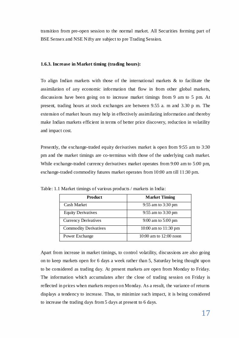
Presently, the exchange-traded equity derivatives market is open from 9:55 am to 3:30
pm and the market timings are co-terminus with those of the underlying cash market.
While exchange-traded currency derivatives market operates from 9:00 am to 5:00 pm,
exchange-traded commodity futures market operates from 10:00 am till 11:30 pm.
Table: 1.1 Market timings of various products / markets in India:
Product Market Timing
Cash Market 9:55 am to 3:30 pm
Equity Derivatives 9:55 am to 3:30 pm
Currency Derivatives 9:00 am to 5:00 pm
Commodity Derivatives 10:00 am to 11:30 pm
Power Exchange 10:00 am to 12:00 noon
Apart from increase in market timings, to control volatility, discussions are also going
on to keep markets open for 6 days a week rather than 5, Saturday being thought upon
to be considered as trading day. At present markets are open from Monday to Friday.
The information which accumulates after the close of trading session on Friday is
reflected in prices when markets reopen on Monday. As a result, the variance of returns
displays a tendency to increase. Thus, to minimize such impact, it is being considered
to increase the trading days from 5 days at present to 6 days.

18
1.6.4 The Market Surveillance system:
Market Surveillance systems have been developed and consolidated on a continuous
basis. Some of the surveillance systems and risk containment measures that have been
put in place are briefly given below:
Risk containment measures in the form of elaborate margining system and linking of
intra-day trading limits and exposure limits to capital adequacy;
Reporting by stock exchanges through periodic and event driven reports;
Establishment of independent surveillance cells in stock exchanges;
Inspection of intermediaries;
Suspension of trading in scrips to prevent market manipulation;
Formation of Inter Exchange Market Surveillance Group for prompt, interactive
and effective decision making on surveillance issues and co-ordination between
stock exchanges;
Implementation of On-line automated surveillance system (Stock Watch
System) at stock exchanges.
Though the minimum measures for risk containment have been specified by the SEBI,
the overall responsibility for risk containment lies with the exchanges. Exchanges have
been directed to take further measures as required. Some additional measures taken by
enforcement of early pay- ins by members with large positions and member-wise adhoc
margins.

19
1.7 Measuring Volatility
Measuring volatility presents some problems. Even simple measures of volatility are
relatively complex. Further, any measurement of volatility requires a lot of information.
Consequently, using any measure of volatility has both advantages and disadvantages.
1.7.1. Standard Deviation:
The most common measure of volatility is standard deviation. To calculate the standard
deviation, we have to first determine a time frame for returns we wish to measure. That
is, we must determine whether we wish to measure the volatility of hourly returns,
daily returns, monthly returns, etc. Standard deviation is a measure of dispersion from
the mean. The more is the deviation , the more is volatility and vice versa.
Where:
rt= rate of return on ith day
= the average rate of return for the month
i= the day identifier for the month ( i.e. for a month , i goes from 1 to 30 or 31)
This model is however still crude and more sophisticated models are frequently used
moving into the area covered by models such as the Exponential Weighted Volatility
models. If we are interested in what the volatility is this instant, the standard deviation
as a measure is of little use.
Stock prices volatility has received a great attention from both academicians and
practitioners over the last two decades because it can be used as a measure of risk in
financial markets. Over recent years, there has been a growth in interest in the
modelling of time-varying stock return volatility. Many economic models assume that
the variance, as a measure of uncertainty, is constant through time. However, empirical

20
evidence rejects this assumption. Economic time series have been found to exhibit
periods of unusually large volatility followed by periods of relative tranquility (Engle,
1982). In such circumstances, the assumption of constant variance (homoskedasticity)
is inappropriate (Nelson,1991). The time series are found to depend on their own past
value (autoregressive), depend on past information (conditional) and exhibit non-
constant variance (heteroskedasticity). It has been found that the stock market volatility
changes with time (i.e., it is ―time-varying‖) and also exhibits positive serial
correlation or ―volatility clustering‖. Large changes tend to be followed by large
changes and small changes tend to be followed by small changes, which mean that
volatility clustering is observed in financial returns data. This implies that the changes
are non-random. These characteristics of time series data can be adequately captured by
ARCH/ GARCH models.
To fully comprehend the GARCH model introduced by Bollerslev (1986) there should be a
clear understanding of the underlying assumptions and models from which GARCH is
derived. In its simplest form, an autoregressive model is a model in which we use the
statistical properties of the past behaviour of a variable y to predict its behaviour in the
future. An overview of these models is given below:
1.7.2. The ARCH Model:
Prior to the ARCH model introduced by Engle (1982), the most common way to
forecast volatility was to determine the standard deviation using a fixed number of the
most recent observations. As we know linear models are based on certain assumptions
and when these assumptions are violated, we use non linear models such as ARCH/
GARCH.
Time series data shows certain characteristics like heteroskedasticity (non constant
variance), volatility clustering, leptokurtosis and reversion towards the mean. Linear
models are not able to capture these characteristics of the time series data.

21
The variance of time series data is not constant, i.e. homoskedastic, but rather a
heteroskedastic process, it is unattractive to apply equal weights considering we know
recent events are more relevant. Moreover, it is not beneficial to assume zero weights
for observations prior to the fixed timeframe. The ARCH model overcomes these
assumptions by letting the weights be parameters to be estimated thereby determining
the most appropriate weights to forecast the variance. The Conditional volatility models
such as ARCH & GARCH incorporate time varying second order moments, where the
series at any time period t is decomposed into its conditional mean and conditional
variance. Both conditional mean and conditional variance depends on all past
information available up to period t-1. The acronym ARCH stands for Autoregressive
Conditional Heteroskedasticity. The term heteroskedasticity" refers to changing
volatility (i.e., variance). But it is not the variance itself which changes with time
according to an ARCH model; rather, it is the conditional variance which changes in a
specific way, depending on the available data. The conditional variance quantifies
uncertainty about the future observation.
An ARCH (1) model, where the conditional variance depends only on one lagged
square error term, is given by:
where,
ht= conditional variance
α o = constant term
α 1= weight
e2t-1= lagged squared error term\
We can capture more of the dependence in the conditional variance by increasing the
number of lags, p , giving us an ARCH( p ) model ARCH Shortcomings
Even though the ARCH model is useful but has its own shortcomings. For instance, we
do not know how many lags, p, we should apply for the best results. The potential
number of lags required to capture all of the dependence in the conditional variance
could be very large thus making the model not very parsimonious.
22
Intuitively, the more parameters we have in the model, the more likely it will be that
one of them will have a negative estimated value.
1.7.3 The GARCH Model:
Empirically, the family of GARCH (generalized ARCH) models has been very
successful in describing the financial data. ARCH and GARCH models treat
heteroskedasticity as a variance to be modeled. Of these models, the GARCH (1, 1) is
often considered by most investigators to be an excellent model for estimating
conditional volatility for a wide range of financial data (Bollerslev, Ray and Kenneth,
1992).
The GARCH specification, firstly proposed by Bollerslev (1986), formulates the serial
dependence of volatility and incorporates the past observations into the future
volatility. GARCH model was first used to model the autoregressive and time varying
nature of Inflation.
GARCH model overcomes the limitations of the ARCH model. Unlike the ARCH
model, the Generalized Autoregressive Centralized Heteroskedasticity model
(GARCH), introduced by Bollerslev (1986) only has three parameters that allows for an
infinite number of squared errors to influence the current conditional variance. This
makes it much more parsimonious than the ARCH model which is why it is widely
employed in practice. Like the ARCH model, the conditional variance determined
through GARCH is a weighted average of past squared residuals. However, the weights
decline gradually but they never reach zero. Essentially, the GARCH model allows the
conditional variance to be dependent upon previous own lags. Using the GARCH
approach, the conditional standard deviation is the measure of volatility, and
distinguishes between the predictable and unpredictable elements in the price process.
This leaves only the stochastic component and is hence a more accurate measure of the
actual risk associated with the price.

23
The GARCH (1, 1) model is given by:
GARCH Shortcomings
Though, in most of the cases, the ARCH and GARCH models are apparently successful
in estimating and forecasting the volatility of the financial time series data, they cannot
capture some of the important features of the data. The most interesting feature not
addressed by these models is the ―leverage effect‖ where the conditional variance
tends to respond asymmetrically to positive and negative shocks in returns. They fail to
capture the fat-tail property of financial data. This has lead to the use of non-normal
distributions (Student-t, Generalized Error Distribution and Skewed Student-t ), within
many nonlinear extensions of the GARCH model which have been proposed. Such as
the Exponential GARCH (EGARCH) of Nelson (1991) the so-called GJR model of
Glosten, Jagannathan, and Runkle (1993) and the Asymmetric Power ARCH
(APARCH) of Ding, Granger, and Engle (1993), to better model the fat-tailed (the
excess kurtosis), skewness and leverage effect characteristics.
Both ARCH and GARCH fail to capture this fact and as such may not produce accurate
forecasts. Recent models building on ARCH and GARCH such as the Threshold
ARCH (TARCH), Exponential GARCH (EGARCH) model have tried to overcome this
problem. However, in the present study we are not concerned about the asymmetries of
the data. The study utilizes GARCH (1,1) equation to model the volatility of the Indian
stock market.
1.8 Motivation of the Study: Generally, two types of arguments prevail in the existing literature. One school of thought
argues that derivatives trading increases stock market volatility due to high degree of
leverage, low transaction costs and hence increases speculation & destabilizes the market.
On the other hand, another school of thought claims that futures market plays an important
24
role in price discovery, enhances market efficiency and reduces asymmetry information of
spot market and has beneficial effect on the underlying cash market. This gives rise to the
controversy among the researchers, academicians and investors on the effect of derivatives
on the underlying market volatility.
A lot of studies have been made to study the effect of index futures on stock market
volatility. Not many studies analyse the impact of futures trading in individual stocks
on the volatility of the underlying. The studies which have been made previously
produce mixed results. The results varied depending on the time period studied and the
country studied.
Most of the studies made earlier considered a short time frame for study. This study
makes an attempt to provide generalizations about the impact of derivatives on stock
market volatility in India by studying the nature of volatility over a longer frame of
time. The present study is focused to know the impact of derivatives (both Index
Futures & Stock Futures) on the volatility of cash market in In

25
1.9 Reference
Narasimham Committee Report (1992) on financial system.
L. C. Gupta Committee Report (1997) In India, derivatives were introduced in a
phased manner after the recommendations of
J.R. Varma Committee Report. It is mostly consistent with the IOSCO(International
Organization of Securities Commission) principles and addresses the common
concerns of investor protection, market efficiency and integrity and financial integrity.

26
REVIEW OF LITERATURE
There has been a vast academic research to access whether or not there is excess volatility in
financial markets and whether or not recent financial market developments pose a threat to
financial market stability. One of these financial market developments has been the
introduction of derivatives trading on the Indian Stock Exchanges. Derivatives have been
introduced on the Indian stock exchanges with the main purpose to contain the volatility of
the Stock Market. Many studies have been conducted to find an answer to the question as to
whether derivatives have been successful in containing the volatility of the Indian Stock
Market.
This study is related to assessing the impact of both index futures & stock futures on the
volatility of the Indian spot market. With respect to futures trading, most of the studies are
related to index futures and very few studies are related to study the impact of SSFs on
volatility. Further, the studies which relate to assessing the impact of index futures
trading on the return volatility of the underlying covered a very short frame of time & the
studies which relate to assessing impact of individual stock futures trading on the return
volatility of the underlying generally consider a small sample of stocks.
As regards market efficiency, most of the studies which relate to index futures report an
increase in market efficiency after introduction of index futures.
A brief review of the studies made on this subject has been presented below.
Gulen and Mayhew (2000) Examine stock market volatility before and after the
introduction of index futures in 25 countries. They find that index futures had no significant
effect on the spot markets in all the countries excluding US and Japan. They also find that
spot volatility was independent of changes in futures trading in 18 countries, and that spot
volatility is negatively influenced by uninformed futures volume in Austria and the UK.
Bologna and Cavallo (2002) examine the effect of the introduction of stock index futures on
the volatility of the Italian spot market, and find a reduction in spot market volatility and
enhanced market efficiency. They conclude that increased impact of recent news and a

27
reduced effect of the uncertainty originating from the old news were the main reasons for this
phenomenon.
Chiang and Wang (2002) Investigate the impact of Taiwan Index futures trading on spot
price volatility using GJR GARCH model and conclude that the trading of TAIEX futures
had a major impact on spot price volatility, while the trading of MSCI Taiwan did not. They
conclude that the increase in asymmetric response behaviour following the beginning of the
trading of two index futures reflects the fact that a major proportion of the investors in TSE
Asian Journal of Finance & Accounting ISSN 1946-052X 2013, Vol. 5, No. 1
www.macrothink.org/ajfa 294 are non- institutional investors who are generally un- informed
and are prone to over react to the bad news. The introduction of the TAIEX futures trading
improves the efficiency of information transmission from futures to spot markets. Raju and
Karande (2003) find a reduction in spot market volatility after the introduction of index
futures.
Golaka C Nath (2003) Investigates behaviour of stock Market volatility after introduction of
derivatives by employing GARCH model. Using a sample of 20 stocks taken randomly from
the NIFTY, he observes that for most of the stocks, the volatility comes down in the post
derivative period while for only few stocks in the sample the volatility in the post derivatives
remains same or increases marginally. Thenmozhi and Thomas (2004) conclude that there is
a reduction in volatility in the underlying stock market and increased market efficiency
following the launch of NIFTY-linked futures.
Pok and Poshakwale (2004) Study the impact of the futures trading on spot market
volatility. They used data from both the underlying and non-underlying stocks of Malaysian
stock market. They used GARCH to test time varying volatility and volatility clustering in
data. They conclude that the initiation of futures trading increases spot market volatility and
the flow of information to the spot market. The underlying stocks respond more to recent
news whereas the non-underlying stocks respond to old news. Antoniou et al. (2005)
examined the relationship between index futures and their underlying markets. Vipul (2006)
investigate the effect of futures trading on volatility in Nifty and in individual stocks using
data for the period from 1998 to 2004. Using GARCH model to capture volatility clustering
28
phenomena in the data, he concludes that introduction of derivatives trading does not
destabilize the stock market.
Mallikarjunappa, T., and Afsal, E.M., (2008) Studied the impact of derivatives (futures
and options) on stock market volatility using a broad based index i.e. S&P CNX Nifty. To
account for heteroskedasticity in the return series GARCH (1, 1) model with dummy
variables has been used in the conditional variance equation. As opposed to their previous
study, this study reported that derivatives have made no impact on the spot market volatility
but the nature of the volatility patterns has altered during the post-derivatives period. The
post-derivatives period has shown that the sensitivity of the index returns to market returns
and any day-of-the-week effects have disappeared.
Marta Casas & Cepeda Edilberto(2008) Explained the ARCH, GARCH, and EGARCH
models and the estimation of their parameters using maximum likelihood technique. The
study concluded that GARCH (1,2) best explains the performance of stock prices and
EGARCH (2,1) best explains the returns series. Ramon L. Haydee (2008) in his study
developed the statistical model to forecast the volatility feature of Philippine inflation from
1995 to August 2007. The study has employed the Autoregressive Moving Average
(ARMA model and then included the Seasonal ARMA (SARMA) model to account for
seasonality in the mean equation. The variance equation has been formulated as the
Generalized Autoregressive Conditional Heteroskedasticity process.
Bansal Nikunj (2009) Analysed the impact of introduction of derivatives on thevolatility of
Indian stock market through ARCH/GARCH technique using S&P CNX NIFTY as a proxy
for Indian market. He has analysed the conditional volatility of interday market returns
before and after the introduction of derivatives using GARCH model. He has found that
derivatives trading has reduced the volatility of the Indian stock market.
Singh Gurcharan & Kansal Saloni (2010) examined the impact of financial derivatives
trading on the volatility of Indian stock market using Standard Deviation as a measure of
volatility. S& P CNX Nifty index has been used as a proxy for stock market and period
covered under the study varies from 1995-1996 to 2008-09 on the financial year basis. The
findings suggest that derivativestrading has reduced the volatility. The decrease in volatility

29
has been mainly attributed to the fact that derivatives markets attract an additional set of
traders to the market, which lead to increase in the trading volume. With the increase in
trading volume, underlying market stock prices reflect greater liquidity and market becomes
more stable.
Ajay Kumar Panda & KoustubhKanti Ray (2011) Analysed the effect of the introduction
of derivatives on the volatility of the Indian stock exchange by using GARCH (1,1) model.
They have found that there has been a change in structure of volatility after implementation of
derivatives and volatility persists for long in post derivatives period as compared to pre
derivatives period. They have also found that most of the stocks have become disintegrated
with market benchmark index after introduction of derivatives.
Kaur Gurpreet (2011) Examined the volatility in the Indian stock market after the
introduction of futures and option contracts. Various volatility forecasting approaches have
been used such as ARCH, GARCH and EGARCH models using the data for a sample period
of 10 years from April 1997 to March 2010. Closing prices of NSE Nifty 50 index have been
used as a proxy for stock market return. The conditional volatility of inter day market returns
before and after the introduction of derivatives products have been estimated with the
GARCH model. The analysis has concluded that the derivatives trading has enhanced the
efficiency of the stock market by reducing the spot market volatility and by enhancing the
liquidity.
Khan, Shah and Khan (2011) examined the Single Stock Futures‘ contracts trading on the
Karachi Stock Exchange and investigated the changes in the return volatility of the underlying
stocks using an augmented GJR-GARCH model as well the more traditional measures of
return volatility. Mixed results have been found for both the SSFs- listed stocks and the
sample of control group stocks in terms of changes in volatility of daily stock returns in the
post-futures periods using traditional measures of return volatility as well as the econometric
investigations. Hence, no conclusive evidences of single stock futures as having caused
changes in the return volatility of the underlying stocks have been found.
30
Suhasini Subramanian (2012) theoretically examined the impact of index futures on
volatility and noise trading. She has analysed contrasting theoretical approaches and empirical
evidence relating to the issue. The paper has concluded that the issue remains unresolved,
despite the many years of research that have gone into investigating the impact of index
futures. The policymaking implications and possible regulatory measures associated with
index futures have also been discussed.
A lot of studies related to different countries have been made to study the relation between
derivatives trading & volatility. Many studies are based on the Indian stock market as well.
But there is no consensus opinion about the impact of derivatives on the volatility of the
underlying stock market as reported by different studies related to India & other countries as
well. However, these studies covered a short span of time and considered a small sample of
stocks.

31
2.2 Reference
Gulen and Mayhew (2000) Examine stock market volatility before and after the
introduction of index futures in 25 countries.
Chiang and Wang (2002) Investigate the impact of Taiwan Index futures trading on
spot price volatility using GJR GARCH model and conclude that the trading of TAIEX
futures had a major impact on spot price volatility
Golaka C Nath (2003) Investigates behaviour of stock Market volatility after
introduction of derivatives by employing GARCH model. Using a sample of 20 stocks
taken randomly from the NIFTY
Pok and Poshakwale (2004) Study the impact of the futures trading on spot market
volatility. They used data from both the underlying and non-underlying stocks of
Malaysian stock market.
Mallikarjunappa, T., and Afsal, E.M., (2008) Studied the impact of derivatives
(futures and options) on stock market volatility using a broad based index i.e. S&P
CNX Nifty.
Marta Casas & Cepeda Edilberto(2008) Explained the ARCH, GARCH, and
EGARCH models and the estimation of their parameters using maximum likelihood
technique
Bansal Nikunj (2009) Analyzed the impact of introduction of derivatives on
thevolatility of Indian stock market through ARCH/GARCH technique using S&P
CNX NIFTY as a proxy for Indian market.
Singh Gurcharan & Kansal Saloni (2010) Examined the impact of financial
derivatives trading on the volatility of Indian stock market using Standard Deviation as
a measure of volatility
32
Ajay Kumar Panda & KoustubhKanti Ray (2011) Analyzed the effect of the
introduction of derivatives on the volatility of the Indian stock exchange by using
GARCH (1,1) model.
Kaur Gurpreet (2011) Examined the volatility in the Indian stock market after the
introduction of futures and option contracts.
Safi Ullah Khan, Attaullah Shah & Zaheer Abbas (2011) Examined the Single
Stock Futures‘ contracts trading on the Karachi Stock Exchange and investigated the
changes in the return volatility of the underlying stocks using an augmented GJR-
GARCH model
Suhasini Subramanian (2012) theoretically examined the impact of index futures on
volatility and noise trading.
33
RESEARCH METHODOLOGY
3.1. Statement of the problem:
One of the motives for introducing derivatives in India had been to contain the stock
market volatility. The perception that futures market can lead to decline in volatility in
spot market is common. However, the converse is also true. As a result, the impact of
trading derivatives on the volatility of spot market is widely debated and the role of
derivatives trading has been the focus of ample recent attention. Increased regulation
on derivatives has been put into practice, regardless of the lack of reliable statistical
evidence that derivatives trading is associated with change in volatility.
The sizeable blame for 2008 US subprime crisis is also put on derivatives. However we
cannot disregard the benefits of derivatives trading as it plays an important role in price
discovery, portfolio diversification and hedging. Some experts in financial markets also
hold a view that derivatives markets solely create market efficiency and hence, find no
ground for regulation within the financial sector and derivatives trading. There are still
disagreements on what role derivatives trading play regarding the stock market
volatility. A lot of studies have been previously made to address this issue but they
produce contradictory results.
Taking into consideration the above factors there is a need to study the impact of
derivatives contracts on Indian market.
The focus area of this thesis is to investigate the role of Index futures & Stock futures
trading on the volatility of the Indian spot markets. The aim of this study is to bring
perspectives to the ongoing debate about the role of derivatives in capital markets.
Thus, the main research question of this thesis is:
‘What is the impact of index futures & stock futures trading on the Indian spot market
volatility?’

34
3.2. Objectives of the study:
The study has been made to fulfill the following objectives:
1.1 To study comparative effect of future contract on stock expected return in the stock
market.
1.2 To study comparative effect of future contract on stock expected price volatility on
stock.
3.3 Hypotheses of the Study:
Based on the objectives of the study, following Null hypotheses have been
constructed to be proved:
Ho1 : There is a no effect of future contract on expected stock return in the stock
Market.
Ho2: There is an effect of future contract on expected stock return in the stock market.
Ho3: There is no any effect of future contract on expected stock price volatility on
Stock.
Ho4: There is an effect of future contract on expected stock price volatility on stock.
3.4. Research design:
Research design is considered as a "blueprint" for research, dealing with at least four
problems: which questions to study, which data are relevant, what data to collect, and
how to analyze the results.

35
The present study utilizes Descriptive Research Design. Descriptive research design
is a scientific method which involves observing and describing the behavior of a
subject without influencing it in any way. Though the study is primarily descriptive in
nature, it also utilizes
Experimental research design where we have controlled the impact of other macro
economic factors on volatility. Therefore, the research design used in this study is
“quantitative, non-experimental and descriptive”.
3.4.1. Data Collection
The historical stock price time series data & the data on indices have been collected
from the official website of National Stock Exchange of India i.e. www.nseindia.com.
And capital line. Other sources of data collection include various books, newspapers,
journals, & internet.
The data set comprises of time series data on 75 individual stocks and 2 indices from
National Stock Exchange (NSE) of India. NSE is India’s leading stock exchange and
records highest trading volume in the derivatives segment. It is value of present future
price in stock. and 75 stock is not present in future price. total data is taken 150
companies from 1st, April 2013 to 31st, March 2014 stock prices.
3.4.2. Sample Selection:
The samples have been selected using the following methodology:
1. Stocks on which derivatives are available:
The study incorporates a sample of 150 such stocks on which derivatives are available.
Derivatives are available at NSE on approximately 75 individual scrip.

36
The study incorporates 75 such stocks on which no derivatives are available. The
sample has been selected as follows:
2. Index on which derivatives are available:
As far as indices are concerned, Nifty has been used for the purpose of study. As a
benchmark index, the Nifty Index can be treated as a true replica of the Indian
derivatives market.
The two indices are stocks. i.e. a stock is present in future price and a stock is not
future price both data is taken same time in capital line.
3.5. Software’s used: The data has been analysed using Eviews 5.1 and spss softwares.
3.6. Statistical tools: The following statistical tools have been used in the study
3.6.1. The ARCH Model:
Under the ARCH model the „autocorrelation in volatility‟ is modeled by allowing the
conditional variance of the error term, to depend on the immediately previous value of
the squared error. Thus, the conditional variance is regressed on constant and lagged
values of the squared error term obtained from the mean equation.
Let the mean equation of the ARCH model follow an AR(1) process, given by:
Where :
The is the white noise process with mean=0 and variance=1
The conditional variance is given by:
37
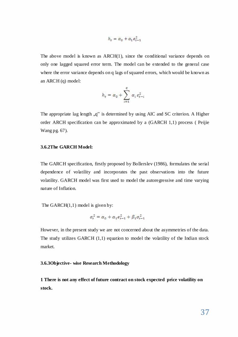
The above model is known as ARCH(1), since the conditional variance depends on
only one lagged squared error term. The model can be extended to the general case
where the error variance depends on q lags of squared errors, which would be known as
an ARCH (q) model:
The appropriate lag length „q‟ is determined by using AIC and SC criterion. A Higher
order ARCH specification can be approximated by a (GARCH 1,1) process ( Peijie
Wang pg. 67).
3.6.2The GARCH Model:
The GARCH specification, firstly proposed by Bollerslev (1986), formulates the serial
dependence of volatility and incorporates the past observations into the future
volatility. GARCH model was first used to model the autoregressive and time varying
nature of Inflation.
The GARCH(1,1) model is given by:
However, in the present study we are not concerned about the asymmetries of the data.
The study utilizes GARCH (1,1) equation to model the volatility of the Indian stock
market.
3.6.3Objective- wise Research Methodology
1 There is not any effect of future contract on stock expected price volatility on
stock.

38
In order to estimate volatility of the Indian Stock Market, GARCH model has been
formulated as follows:
Impact of Individual Stock Futures (SSF) on spot market volatility: In order to analyze
the impact of introduction of individual stock futures on spot market, daily closing
prices of all the sampled companies on which derivatives are traded have been
examined. These closing prices have been converted into logarithmic returns to make
them stationary. The mean equation has been specified by the baseline scenario, AR
After satisfying about the characteristics of the time series data, GARCH (1,1) model
has been used.
2. There is a effect of future contract on expected stock return in the stock market
To study the impact of derivatives trading on price discovery, we have divided the
entire series into two parts i.e.
Future Contract Present
Future Contract not Present
A comparison of ARCH and GARCH term in futures contract present and future
contract not present the impact of derivatives on price discover. Nifty index has been
used to price of Indian stock market.
1. The return series has been calculated from closing price for present value of future
price and not future price.
2. After a mean equation has been formulated as ARMA (1, 1) model, the residuals of
the model have been tested for the presence autocorrelation and heteroskedasticity.
3. Now error terms have been tested for any ARCH effects using ARCH LM test
testing the null hypothesis of no heteroskedasticity. A low p value rejected the null
hypothesis of no heteroskedasticity. This indicated the presence of
heteroskedasticity in the error terms supporting the use of ARCH/GARCH class
models to capture such characteristics.

39
4. Next, we fitted the most suitable GARCH (p, q) model specification with the help
of Akaike and Schwarz information criterion. AIC was least for GARCH (1,1)
model. Hence, the variance equation has been formulated as GARCH (1, 1) model
to capture the Indian Stock Market Volatility.
In order to estimate the level of volatility prevailing in the Indian stock market
unconditional variance has been estimated as follows:
Where:
Derivatives are assumed to play an important role in price discovery by increasing the
speed of information transmission. Thus a larger ARCH term and a smaller GARCH
term in post derivatives period would be the preferred outcome to explain the role of
derivatives on price discovery.
3.7 Limitations of the Study
1. The daily unadjusted close prices have been used and computed the day-to-day
changes, either as logarithmic returns. However, the unadjusted close prices did
not adjust for stock splits and dividend payments.
2. The analysis is confined to Secondary Data only.
3. All the limitations of the models deployed are applicable to this study also.
4. The study has not attempted to travel beyond GARCH-type models to predict
the market volatility and also only symmetric GARCH type models have been
used. The asymmetries in volatility have not been taken into account.

40
IMPACT OF FUTURES ON EXPECTED PRICE AND RETURN
An important aspect of derivatives trading that has been broadly discussed in the
literature refers to the aspect of information transmission. The mechanism of
information transmission plays a central role in achieving financial market efficiency.
The quicker, the new information is incorporated in asset prices, the higher is the
informational efficiency of financial markets. This process is also termed as price
discovery.
Derivatives are assumed to play an important role in price discovery because they offer
market participants the possibility to price their expectations of future states of the
economy and the underlying asset. Thus, expectations about future prices of the
underlying become measurable and this additional information is revealed to other
market participants acting in the derivatives and cash markets. This follows from the
fact that prices in derivatives and cash markets value the same underlying asset. They
therefore, are linked and will move together if markets are at least partly efficient.
Thus, the information about future prices of the underlying incorporated in the price of
the derivative can be shared free of charge by other market participants who have to
make their investment, production or consumption decisions. With the help of an
efficient price discovery process a more efficient inter temporal allocation of resources
can be achieved which is regarded as socially beneficial.
4.1 Impact of futures on price discovery:
To study the impact of index futures in discovering spot prices, daily closing prices of S
Nifty index have been used from 1st April 2013 to 31st March 2014. These closing
prices have been converted into stationary return series by taking logarithmic
differences.
4.1.1 The ARCH Model:
Under the ARCH model the „autocorrelation in volatility‟ is modeled by allowing the
conditional variance of the error term, to depend on the immediately previous value of

41
the squared error. Thus, the conditional variance is regressed on constant and lagged
values of the squared error term obtained from the mean equation.
Let the mean equation of the ARCH model follow an AR(1) process, given by:
Where :
The is the white noise process with mean=0 and variance=1
The conditional variance is given by:
The above model is known as ARCH(1), since the conditional variance depends on
only one lagged squared error term. The model can be extended to the general case
where the error variance depends on q lags of squared errors, which would be known as
an ARCH (q) model:
The appropriate lag length „q‟ is determined by using AIC and SC criterion. A Higher
order ARCH specification can be approximated by a (GARCH 1,1) process ( Peijie
Wang pg. 67).
4.1.2 The GARCH Model:
GARCH model overcomes the limitations of the ARCH model. Unlike the ARCH
model, the Generalized Autoregressive Centralized Heteroskedasticity model
(GARCH), introduced by Bollerslev (1986) only has three parameters that allows for an
infinite number of squared errors to influence the current conditional variance. This
makes it much more parsimonious than the ARCH model which is why it is widely
employed in practice. Like the ARCH model, the conditional variance determined
through GARCH is a weighted average of past squared residuals.

42
However, the weights decline gradually but they never reach zero. Essentially, the
GARCH model allows the conditional variance to be dependent upon previous own
lags. Using the GARCH approach, the conditional standard deviation is the measure of
volatility, and distinguishes between the predictable and unpredictable elements in the
price process. This leaves only the stochastic component and is hence a more accurate
measure of the actual risk associated with the price.
The GARCH(1,1) model is given by:
Both ARCH and GARCH fail to capture this fact and as such may not produce accurate
forecasts. Recent models building on ARCH and GARCH such as the Threshold
ARCH (TARCH), Exponential GARCH (EGARCH) model have tried to overcome this
problem. However, in the present study we are not concerned about the asymmetries of
the data. The study utilizes GARCH (1,1) equation to model the volatility of the Indian
stock market.
4.1.3 Independent samples t-test
The independent samples t-test is used when two separate sets of independent and
identically distributed samples are obtained, one from each of the two populations
being compared. For example, suppose we are evaluating the effect of a medical
treatment, and we enroll 100 subjects into our study, then randomly assign 50 subjects
to the treatment group and 50 subjects to the control group. In this case, we have two
independent samples and would use the unpaired form of the t-test. The randomization
is not essential here – if we contacted 100 people by phone and obtained each person's
age and gender, and then used a two-sample t-test to see whether the mean ages differ
by gender, this would also be an independent samples t-test, even though the data are
observational

43
Equal sample sizes, equal variance
This test is only used when both:
• the two sample sizes (that is, the number, n, of participants of each group) are
equal;
• it can be assumed that the two distributions have the same variance.
Violations of these assumptions are discussed below.
The t statistic to test whether the means are different can be calculated as follows:
where
Here is the grand standard deviation (or pooled standard deviation), 1 = group
one, 2 = group two. and are the unbiased estimators of the variances of the two
samples. The denominator of t is the standard error of the difference between two
means.
For significance testing, the degrees of freedom for this test is 2n − 2 where n is the
number of participants in each group.

44
Table 4.2 Levene statistics for equality of variances
Variable F-value Sig. Assumption
Variance 3.846 0.052 Supported
Residual error 11.260 0.001 Violated
Price mean 0.122 0.727 Violated
Table 4.3: independent smaple
Variable T df Sig. (2-tailed)
Variance 1.066 148 .288
Residual error -4.278 133.705 .000
Price mean -1.788 148 .076
Interpretation:
Variance:
In variance null hypothesis is accepted it means there is not an effect of future contract
on expected stock return in the spot market.
Table 4.1 Group Statistics
Codin
g N Mean
Std.
Deviation
Std. Error
Mean
Var1 1 75 .5451 .44994 .05230
2 75 .4764 .33256 .03815
Meant1 1 75 .9654 .06986 .00812
2 75 .9856 .06863 .00787
Res1 1 75 .1484 .20052 .02331
2 75 .3221 .28970 .03323
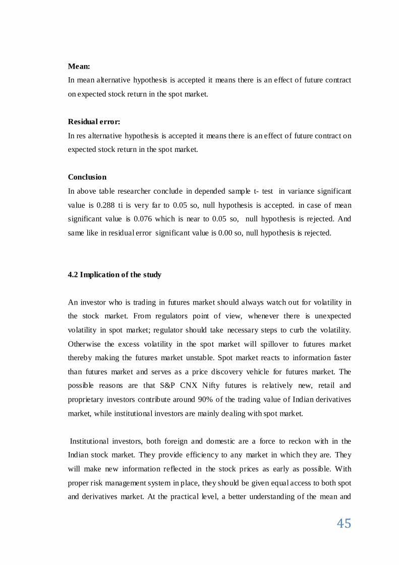
45
Mean:
In mean alternative hypothesis is accepted it means there is an effect of future contract
on expected stock return in the spot market.
Residual error:
In res alternative hypothesis is accepted it means there is an effect of future contract on
expected stock return in the spot market.
Conclusion
In above table researcher conclude in depended sample t- test in variance significant
value is 0.288 ti is very far to 0.05 so, null hypothesis is accepted. in case of mean
significant value is 0.076 which is near to 0.05 so, null hypothesis is rejected. And
same like in residual error significant value is 0.00 so, null hypothesis is rejected.
4.2 Implication of the study
An investor who is trading in futures market should always watch out for volatility in
the stock market. From regulators point of view, whenever there is unexpected
volatility in spot market; regulator should take necessary steps to curb the volatility.
Otherwise the excess volatility in the spot market will spillover to futures market
thereby making the futures market unstable. Spot market reacts to information faster
than futures market and serves as a price discovery vehicle for futures market. The
possible reasons are that S&P CNX Nifty futures is relatively new, retail and
proprietary investors contribute around 90% of the trading value of Indian derivatives
market, while institutional investors are mainly dealing with spot market.
Institutional investors, both foreign and domestic are a force to reckon with in the
Indian stock market. They provide efficiency to any market in which they are. They
will make new information reflected in the stock prices as early as possible. With
proper risk management system in place, they should be given equal access to both spot
and derivatives market. At the practical level, a better understanding of the mean and

46
variance dynamics of the spot and futures market can improve risk management and
investment decisions of the market agents.
Volatility estimation is important for several reasons and for different people in the
market pricing of securities is supposed to be dependent on volatility of each asset.
Market prices tend to exhibit periods of high and low volatility. This sort of behaviour
is called volatility clustering. Volatility clustering is tested for sample series, which
means “large changes tend to be followed by large changes, of either sign, and small
changes tend to be followed by small changes.”

47
FINDINGS
There has been a change in level of volatility in Indian stock market because of future
contract variance significant. Trading in Index futures have an impact on price
discovery. The index futures reported increase in informational efficiency by reporting
an increase in ARCH term & GARCH term and hence play role in price discovery.
The persistence in volatility has increased in the derivatives as a result of t- test while it
has shown for Index futures.
The empirical findings confirmed the fact that there has been no increase in volatility as
a result of derivatives trading. Volatility coefficient has neither shown an increase in
case of index futures.
The volatility in Indian stock market exhibits the characteristics with respect to the
Stylized features like autocorrelation, volatility clustering, asymmetry and persistence
in its daily return. The impact of financial derivatives on the volatility of NSE Nifty is
significant under all the models. It is due to the derivatives.
Future contract effect on expected retune in sport market and price volatility in Indian
stock market.

48
CONCLUSION
In order to contribute to the literature of Indian financial market, the study analyses the
impact of Index Futures trading & Single Stock Futures (SSFs) trading on stock market
volatility in India using GARCH(1,1) model. To study the impact of index futures
trading on volatility, daily closing prices of S&P CNX NIFTY have been used.
The data set comprises of time series data on 75 individual stocks and 2 indices from
National Stock Exchange (NSE) of India. NSE is India’s leading stock exchange and
records highest trading volume in the derivatives segment. It is value of present future
price in stock. and 75 stock is not present in future price. total data is taken 150
companies from 1st, April 2013 to 31st, March 2014 sock pries.
The preliminary analysis of data set suggests that volatility in the Indian stock market is
time varying in nature, persist to form clusters and has a long memory process. These
findings of the data characteristics have been consistent with previous studies of Indian
capital markets and justify the application of GARCH type models for the case. In
general, regarding the impact of derivatives on stock market volatility, index futures
alone have led to a increase in volatility in the expected pries and also help in price
discovery by improving the information efficiency.

49
BIBLIOGRAPHY
Narasimham Committee Report (1992) on financial system.
L. C. Gupta Committee Report (1997) In India, derivatives were introduced in a phased
manner after the recommendations of
J.R. Varma Committee Report. It is mostly consistent with the IOSCO(International
Organization of Securities Commission) principles and addresses the common concerns of
investor protection, market efficiency and integrity and financial integrity.
Gulen and Mayhew (2000) Examine stock market volatility before and after the introduction
of index futures in 25 countries.
Chiang and Wang (2002) Investigate the impact of Taiwan Index futures trading on spot
price volatility using GJR GARCH model and conclude that the trading of TAIEX futures
had a major impact on spot price volatility
Golaka C Nath (2003) Investigates behaviour of stock Market volatility after introduction of
derivatives by employing GARCH model. Using a sample of 20 stocks taken randomly from
the NIFTY
Pok and Poshakwale (2004) Study the impact of the futures trading on spot market
volatility. They used data from both the underlying and non-underlying stocks of Malaysian
stock market.

50
Mallikarjunappa, T., and Afsal, E.M., (2008) studied the impact of derivatives (futures
and options) on stock market volatility using a broad based index i.e. S&P CNX Nifty.
Marta Casas & Cepeda Edilberto(2008) explained the ARCH, GARCH, and EGARCH
models and the estimation of their parameters using maximum likelihood technique
Bansal Nikunj (2009) analysed the impact of introduction of derivatives on thevolatility
of Indian stock market through ARCH/GARCH technique using S&P CNX NIFTY as a
proxy for Indian market.
Singh Gurcharan & Kansal Saloni (2010) examined the impact of financial derivatives
trading on the volatility of Indian stock market using Standard Deviation as a measure of
volatility
Ajay Kumar Panda & KoustubhKanti Ray (2011) analysed the effect of the introduction
of derivatives on the volatility of the Indian stock exchange by using GARCH (1,1) model.
Kaur Gurpreet (2011) examined the volatility in the Indian stock market after the
introduction of futures and option contracts.
Safi Ullah Khan, Attaullah Shah & Zaheer Abbas (2011) examined the Single Stock
Futures‘ contracts trading on the Karachi Stock Exchange and investigated the changes in the
return volatility of the underlying stocks using an augmented GJR-GARCH model
Suhasini Subramanian (2012) theoretically examined the impact of index futures on
volatility and noise trading.

51
Books referred: Damodar N. Gujarati (2007), “Basic Econometrics”, Tata Mc. Graw Hill publishers, 4e, pp. 1-396. John Hanke (2009), “Business Forecasting”, Prentice Hall of India, Eastern Economy edition, pp. 381-457. Peijie Wang ( 2009), “ Financial Econometrics”, Roultledge Publishers, 2e, pp. 66-74. Ramu Ramanathan (2002), “Introductory Econometrics with Applications”, 5e, Cengage Learning, Harcourt College Publishers. Richard Harris & Robert Sollis (2006), “ Applied Time Series Modelling & Forecasting”, Wiley Publishers, Student Edition, pp. 213-259. Websites: www.nseindia.com www.capital line .com http://www.futuresindustry.org/volume-.asp
wikipedia.org/wiki/Derivative_(finance) www.bseindia.com/markets/Derivatives/DeriReports/introduction.aspx www.investopedia.com/terms/v/volatility.asp

52
Table: 8.1Company name which have Future Contract:
NO. Name c Series(-1) c Resid(-1)^2 Garch(-1) series01 Hindustan Zinc Ltd 3.439472 0.971384 4.113598 0.335712 0.011539
serioes02 Hindustan Unilever Ltd
7.506528 0.986448 0.683000 0.976704 0.539122
series03 Arvind Ltd 1.166588 0.984015 0.099637 0.047734 1.022195
series04 Grasim Industries Ltd 123.7299 0.954264 207.1573 0.127798 0.751342
series05 Havells India Ltd 18.76919 0.971569 113.9149 0.393402 0.088653
series06 HCL Technologies Ltd 4.113851 0.993465 11.23617 0.100051 0.878833
series07 ICICI Bank Ltd 47.14820 0.954083 756.4248 0.191422 -0.591346
series08 Aurobindo Pharma Ltd 2.047557 0.985552 0.34642 0.037158 0.947901
series09 ACC Ltd 41.78822 0.962444 412.5779 0.162005 -0.28379 series10 Ambuja Cements Ltd 10.01300 0.943017 6.84164 0.170676 0.38789
series11 Adani Ports & Special Economic Zone Ltd
8.211591 0.944201 5.273244 0.16564 0.43185
series12 Hexaware Technologies Ltd
0.704797 0.992018 0.205154 0.231313 0.779429
series13 Axis Bank Ltd 31.08417 0.973976 27.24265 0.047702 0.925287
series14 Indiabulls Real Estate Ltd
1.672113 0.972534 0.13898 0.056114 0.919152
series15 Federal Bank Ltd 1.114688 0.984466 7.300586 0.03324 -0.94811
series16 Andhra Bank -0.097706
1.001925 0.330911 0.305883 0.579186
series17 Hero Moto Corp Ltd 15.01565 0.990827 146.7744 0.134075 0.724671
series18 Ambuja Cements Ltd 10.013 0.943017 5.84164 0.170676 0.38789
series19 Allahabad Bank 0.133743 0.999815 4.158657 0.085454 0.216585
series20 Bank of India 0.186471 0.999913 45.96909 0.27724 -0.11945
series21 Godrej Industries Ltd 14.6708 0.947989 4.559266 0.126945 0.731786

53
series22 GMR Infrastructure Ltd
0.269458 0.987043 0.064079 0.168341 0.643296
series23 Adani Enterprises Ltd 7.424075 0.961783 1.107265 -0.06275 1.02955
series24 GAIL (India) Ltd 15.30812 0.953634 26.09692 0.093552 0.030741
series25 Apollo Hospitals Enterprise Ltd
46.27044 0.944103 27.7463 0.251056 0.694899
series26 Hindalco Industries Ltd
2.454531 0.976174 0.344613 0.105025 0.842304
series27 Asian Paints Ltd 31.42648 0.39449 1.08228 0.05224 0.933747
series28 Adani Power Ltd 0.880103 0.976077 0.153651 0.219332 0.866399
series29 HDFC Bank Ltd 40.93189 0.937784 5.682768 0.057393 0.904381
series30 GlaxoSmithkline Consumer Healthcare Ltd
298.1086 0.930889 323.0831 0.190357 0.80221
series31 Glenmark Pharmaceuticals Ltd
22.39325 0.958199 30.46589 0.98617 0.620256
series32 Hindustan Petroleum Corporation Ltd
2.905801 0.987151 16.80678 0.103028 0.37547
series33 Bajaj Auto Ltd 76.75067 0.959311 9.63855 -0.04005 1.032623
series34 Housing Development Finance Corporation Ltd
63.94876 0.921289 6.707058 0.060845 0.914616
series35 Cipla Ltd 22.86489 0.943277 20.44429 -0.04142 0.501614 series36 Cairn India Ltd 11.52346 0.962604 3.480258 0.205517 0.630131 series37 IDBI Bank Ltd 0.319248 0.995161 0.075613 0.067519 0.896025 series38 Bharat Petroleum
Corporation Ltd 13.68664 0.960806 7.37543 0.074423 0.819591
series39 Biocon Ltd 2.948471 0.989351 2.092181 0.196061 0.785913 series40 Canara Bank 0.711532 0.997195 1.204688 0.82139 0.910937 series41 Colgate-Palmolive
(India) Ltd 58.1929 0.955371 53.25748 0.390868 0.537799
series42 Dabur India Ltd 4.157408 0.973863 0.939486 0.137327 0.738493 series43 Bharti Airtel Ltd 13.90526 0.955439 0.941983 0.035111 0.945955 series44 Divis Laboratories Ltd 12.36889 0.987626 238.6721 0.192284 0.050389 series45 DLF Ltd 1.235894 0.993629 3.769838 0.08669 0.783397 series46 Bata India Ltd 9.281093 0.98767 47.6513 0.043283 0.77387 series47 Idea Cellular Ltd 48585 0.998811 0.906456 0.120709 0.810778 series48 Crompton Greaves Ltd 1.960537 0.978796 2.254513 0.147209 0.585812 series49 IDFC Ltd 0.812216 0.993622 11.15509 0.027472 -0.12816 series50 Coal India Ltd 10.16648 0.964078 0.331181 -0.03559 1.033219
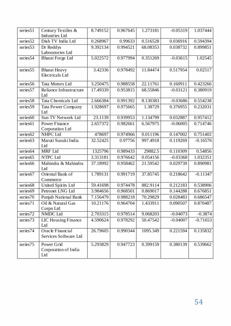
54
series51 Century Textiles & Industries Ltd
8.749152 0.967645 1.273181 -0.05319 1.037444
series52 Dish TV India Ltd 0.268967 0.99633 0.516528 0.036916 0.594394 series53 Dr Reddys
Laboratories Ltd 9.392134 0.994521 68.08353 0.038732 0.899851
series54 Bharat Forge Ltd 5.022572 0.977994 0.351269 -0.03615 1.02545
series55 Bharat Heavy Electricals Ltd
3.42336 0.978492 11.84474 0.517954 0.02517
series56 Tata Motors Ltd 3.250475 0.988558 22.11761 0.160911 0.423266 series57 Reliance Infrastructure
Ltd 17.49339 0.953815 68.55846 -0.03121 0.380919
series58 Tata Chemicals Ltd 2.666384 0.991392 8.130383 -0.03686 0.554238 series59 Tata Power Company
Ltd 1.928697 0.975665 1.38729 0.376955 0.232031
series60 Sun TV Network Ltd 23.1139 0.939953 1.134799 0.032887 0.957412 series61 Power Finance
Corporation Ltd 2.657372 0.982661 6.567975 -0.06005 0.714746
series62 NHPC Ltd 478697 0.974966 0.011196 0.147002 0.751402 series63 Maruti Suzuki India
Ltd 32.52425 0.97756 997.4918 0.119269 -0.16576
series64 MRF Ltd 1325796 0.989433 29882.5 0.110309 0.54856 series65 NTPC Ltd 3.313181 0.976642 0.054156 -0.03368 1.032351 series66 Mahindra & Mahindra
Ltd 37.18992 0.958462 21.59542 0.029739 0.890981
series67 Oriental Bank of Commerce
1.789131 0.991719 37.85745 0.218642 -0.11347
series68 United Spirits Ltd 59.41698 0.974478 882.9114 0.212183 0.538906 series69 Petronet LNG Ltd 3.984656 0.968501 0.869017 0.144288 0.676851 series70 Punjab National Bank 7.156479 0.988218 70.29829 0.028483 0.686547 series71 Oil & Natural Gas
Corpn Ltd 10.21176 0.964704 1.433911 0.090507 0.870487
series72 NMDC Ltd 2.703315 0.978514 9.068203 -0.04073 -0.3874 series73 LIC Housing Finance
Ltd 4.590624 0.978292 50.47542 -0.04007 -0.71653
series74 Oracle Financial Services Software Ltd
26.79605 0.990344 1095.349 0.221594 0.135832
series75 Power Grid Corporation of India Ltd
5.293829 0.947723 0.399159 0.380139 0.539662

55
Table:8.2 Company name which not have Future Contract:
NO. Name c Series(-1) c Resid(1)^2 Garch(-1)
series01 Sundaram Clayton Ltd 8.90661 0.971275 11.87756 0.209547 0.575146
series02 India Nippon Electricals
Ltd
8.082116 0.950879 2.977799 0.502687 0.383477
series03 Federal-Mogul Goetze
(India) Ltd
19.36683 0.902766 1.657395 0.700212 0.212401
series04 Vimta Labs Ltd -0.04623 0.999581 0.02075 0.728361 0.573761
series05 Amtek India Ltd 0.62709 0.990852 2.226699 1.3185 0.100338
series06 Hindalco Industries Ltd 2.454531 0.976174 0.344613 0.105025 0.842304
series07 Lumax Auto
Technologies Ltd
0.098443 1.000092 2.280661 0.124591 0.335485
series08 Munjal Auto Industries
Ltd
0.706469 0.977382 0.442903 0.366442 0.073926
series09 Sona Koyo Steering
Systems Ltd
0.13357 0.985595 0.002979 0.113514 0.866842
series10 Motherson Sumi Systems
Ltd
1.543322 1.543322 10.30637 0.396486 0.062907
series11 Amara Raja Batteries Ltd 5.461465 0.980864 21.91883 0.156852 0.335887
series12 Steel Strips Wheels Ltd 2.805899 0.979966 4.814732 0.864806 0.01319
series13 L G Balakrishnan & Bros
Ltd
2.720091 0.986039 6.408656 0.489043 0.365359
series14 Fiem Industries Ltd 2.752098 0.985633 0.100607 0.350767 0.733785
series15 Wheels India Ltd 35.15626 0.945423 351.4447 0.775407 -0.00999
series16 Hindustan Motors Ltd 0.18674 0.976726 0.026948 0.557748 -0.05688
series17 Ucal Fuel Systems Ltd 0.715903 0.984063 0.359353 0.508808 0.281087
series18 Goa Carbon Ltd 0.880829 0.98829 1.305238 0.758645 0.007433
series19 Autoline Industries Ltd 2.001341 0.973124 0.31582 0.25797 0.74665
series20 Bosch Ltd 349.8441 0.960312 4125.697 0.40782 0.301118
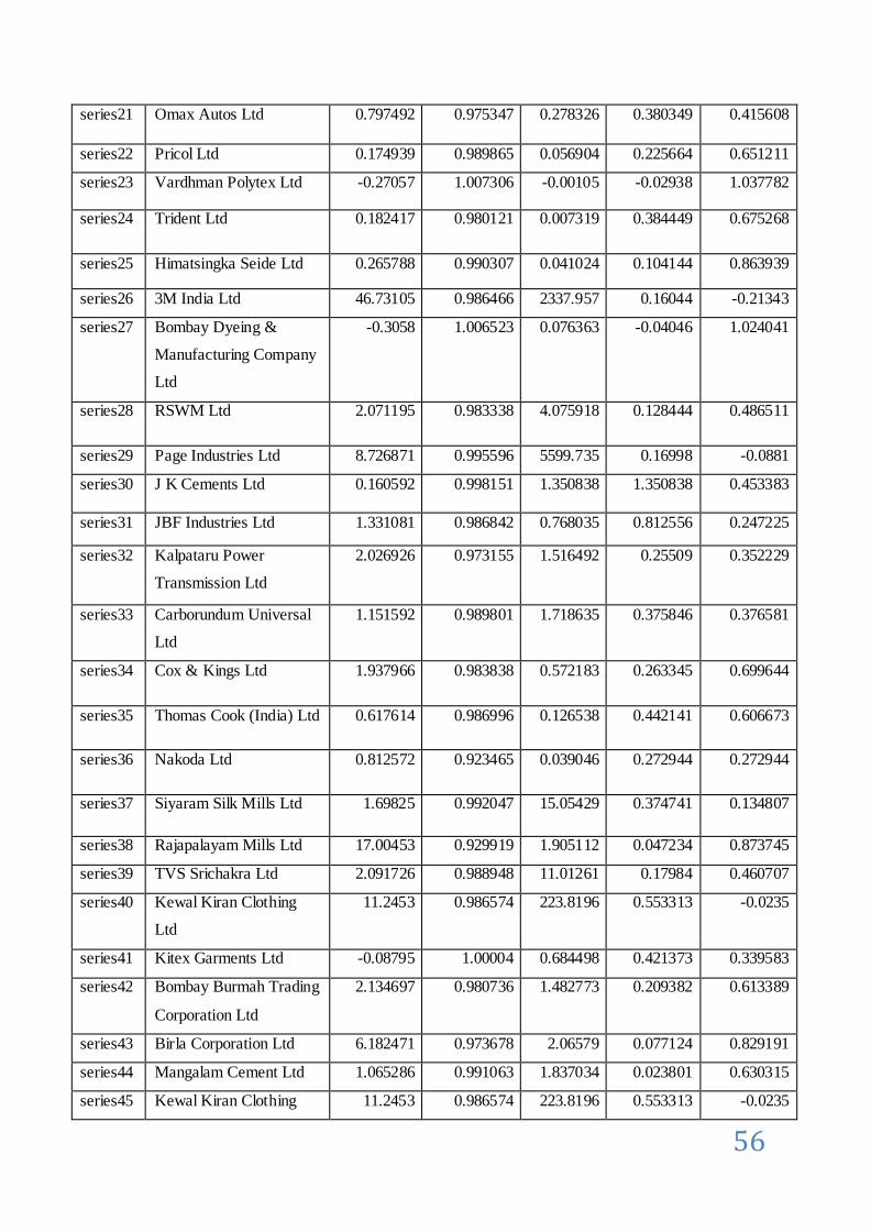
56
series21 Omax Autos Ltd 0.797492 0.975347 0.278326 0.380349 0.415608
series22 Pricol Ltd 0.174939 0.989865 0.056904 0.225664 0.651211
series23 Vardhman Polytex Ltd -0.27057 1.007306 -0.00105 -0.02938 1.037782
series24 Trident Ltd 0.182417 0.980121 0.007319 0.384449 0.675268
series25 Himatsingka Seide Ltd 0.265788 0.990307 0.041024 0.104144 0.863939
series26 3M India Ltd 46.73105 0.986466 2337.957 0.16044 -0.21343
series27 Bombay Dyeing &
Manufacturing Company
Ltd
-0.3058 1.006523 0.076363 -0.04046 1.024041
series28 RSWM Ltd 2.071195 0.983338 4.075918 0.128444 0.486511
series29 Page Industries Ltd 8.726871 0.995596 5599.735 0.16998 -0.0881
series30 J K Cements Ltd 0.160592 0.998151 1.350838 1.350838 0.453383
series31 JBF Industries Ltd 1.331081 0.986842 0.768035 0.812556 0.247225
series32 Kalpataru Power
Transmission Ltd
2.026926 0.973155 1.516492 0.25509 0.352229
series33 Carborundum Universal
Ltd
1.151592 0.989801 1.718635 0.375846 0.376581
series34 Cox & Kings Ltd 1.937966 0.983838 0.572183 0.263345 0.699644
series35 Thomas Cook (India) Ltd 0.617614 0.986996 0.126538 0.442141 0.606673
series36 Nakoda Ltd 0.812572 0.923465 0.039046 0.272944 0.272944
series37 Siyaram Silk Mills Ltd 1.69825 0.992047 15.05429 0.374741 0.134807
series38 Rajapalayam Mills Ltd 17.00453 0.929919 1.905112 0.047234 0.873745
series39 TVS Srichakra Ltd 2.091726 0.988948 11.01261 0.17984 0.460707
series40 Kewal Kiran Clothing
Ltd
11.2453 0.986574 223.8196 0.553313 -0.0235
series41 Kitex Garments Ltd -0.08795 1.00004 0.684498 0.421373 0.339583
series42 Bombay Burmah Trading
Corporation Ltd
2.134697 0.980736 1.482773 0.209382 0.613389
series43 Birla Corporation Ltd 6.182471 0.973678 2.06579 0.077124 0.829191
series44 Mangalam Cement Ltd 1.065286 0.991063 1.837034 0.023801 0.630315
series45 Kewal Kiran Clothing 11.2453 0.986574 223.8196 0.553313 -0.0235
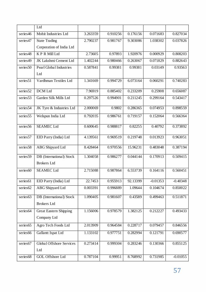
57
Ltd
series46 Mohit Industries Ltd 3.263359 0.910256 0.176156 0.071683 0.827034
series47 State Trading
Corporation of India Ltd
2.790237 0.981767 9.303086 1.038302 0.037826
series48 K P R Mill Ltd 2.73605 0.97893 1.920976 0.000929 0.808203
series49 JK Lakshmi Cement Ltd 1.402244 0.980466 0.263067 0.071829 0.882643
series50 Pearl Global Industries
Ltd
0.587841 0.99381 0.99381 0.03149 0.93563
series51 Vardhman Textiles Ltd 1.341669 0.994729 6.073164 0.060291 0.740283
series52 DCM Ltd 7.96919 0.885402 0.233209 0.25908 0.656087
series53 Garden Silk Mills Ltd 0.297526 0.994901 0.211245 0.299164 0.543417
series54 JK Tyre & Industries Ltd 2.000069 0.9802 0.286365 0.074953 0.898559
series55 Welspun India Ltd 0.792035 0.986761 0.719157 0.152064 0.566364
series56 SEAMEC Ltd 0.600645 0.988817 0.82255 0.40792 0.373892
series57 EID Parry (India) Ltd 4.139561 0.969519 0.219748 0.013923 0.963051
series58 ABG Shipyard Ltd 8.428464 0.970556 15.96231 0.483048 0.387194
series59 DB (International) Stock
Brokers Ltd
1.304058 0.986277 0.044144 0.170913 0.509415
series60 SEAMEC Ltd 2.715088 0.987864 6.553739 0.164116 0.560451
series61 EID Parry (India) Ltd 22.7453 0.955913 92.13399 -0.01353 -0.40348
series62 ABG Shipyard Ltd 0.003391 0.996889 1.09644 0.104674 0.850022
series63 DB (International) Stock
Brokers Ltd
1.090405 0.981607 0.43589 0.499463 0.511871
series64 Great Eastern Shipping
Company Ltd
1.156006 0.978579 1.382125 0.212227 0.493433
series65 Agro Tech Foods Ltd 2.013909 0.964584 0.228717 0.079457 0.846556
series66 Gallantt Ispat Ltd 1.133102 0.977751 0.282994 0.121791 0.690577
series67 Global Offshore Services
Ltd
0.273414 0.999304 0.283246 0.130366 0.855125
series68 GOL Offshore Ltd 0.787104 0.99951 8.768992 0.731985 -0.01055

58
series69 IIFL Holdings Ltd 8.060381 0.971616 35.88788 0.240597 -0.06169
series70 IIFL Holdings Ltd 0.608793 0.99741 1.019989 0.063028 0.871291
series71 Indian Hotels Co Ltd 0.391853 0.993856 0.970394 0.162794 0.478433
series72 Asian Hotels (North) Ltd 1.519304 0.958712 0.195001 0.330315 0.539142
series73 Vivimed Labs Ltd 2.097843 0.962383 0.189332 0.452161 0.458609
series74 Mcleod Russel India Ltd 2.715088 0.987864 6.553739 0.164116 0.560451
series75 The Ramco Cements Ltd 1.066736 0.9966 169.1994 0.304085 -0.15431