Impact of decreased wetlands on microclimate of Kolkata, India

Impact of decreased wetlands on microclimate of Kolkata, India

by

Xia Li

A thesis submitted to the Graduate Faculty of

Auburn University

in partial fulfillment of the

requirements for the Degree of

Master of Science

Auburn, Alabama

August 1, 2015

Keywords: Wetland shrinkage, built-up area expansion, microclimate changes, Kolkata

city, Weather Research and Forecasting (WRF) model

Copyright 2015 by Xia Li

Approved by

Chandana Mitra, Chair, Assistant Professor of Department of Geosciences

Luke Marzen, Professor of Department of Geosciences

Li Dong, Assistant Research Professor of Department of Geosciences

ii

ABSTRACT

The Landsat images were used to assess landuse/landcover (LULC) changes in

Kolkata Metropolitan Development Area (KMDA) from 1990 to 2011 and in East Kolkata

Wetlands (EKWs) from 1972 to 2011using a geographic object-based analysis (GeOBIA)

technique and post-classification comparison. Then, the Weather Research and Forecasting

(WRF) model was applied to investigate impacts of LULC dynamics on micro-climate

using three scenario analyses (real condition scenario; urbanization scenario; and irrigate

cropland expansion scenario). Results suggested that built-up area increased almost twice

in 2011 when comparing it to 1990. The increased area was mainly coursed by conversions

of wetlands and croplands. More specifically, EKWs decreased by 17.9% between 1972

and 2011. Urbanization can greatly increase regional temperature and stimulate sensible

heat fluxes but reduce latent heat fluxes and albedo. On the contrary, the expansion of

irrigated croplands decreased the temperature and sensible heat fluxes but increased latent

heat fluxes and albedo.

iii

Acknowledgments

I would like to thank my major professor Dr. Chandana Mitra for her guidance,

instruction, and support during my study at Auburn University. Her devotion and untiring

effort towards urban and climate research encouraged me to overcome difficulties in my

study and will be valuable for my academic career in the future. I would also like to express

much appreciation to committee members Dr. Luke Marzen and Dr. Li Dong, who are

always willing to offer help and give valuable suggestions to my work.

I would like to send my best regard to my friends. Discussions with Mr. Samriddhi

Shakya on research methods and scientific questions were always motivating and inspiring.

I also want to express my hearty thanks to Ms. Ting Du, Ms. Audrey Smith Hollis, and Mr.

Anthony Hall who helped me so much during my study in the Geosciences department.

I want to thank my parents for their support and help during my study and my life.

Words are not enough to express my gratitude for them. I also want to thank my husband,

Dr. Qichun Yang. Without his unending love and encouragement I could not finish my

thesis. Finally, I want to thank my son, Edward Yang. His lovely face and sweet smile

always gives me confidence to overcome the difficulties I met during my study period.

iv

Table of Contents

ABSTRACT ........................................................................................................................ ii

Acknowledgments.............................................................................................................. iii

List of Tables ..................................................................................................................... vi

List of Figures ................................................................................................................... vii

1. Introduction ..................................................................................................................1

1.1 Objectives ...............................................................................................................2

1.2 Thesis Structure ......................................................................................................3

1.3 Reference ................................................................................................................4

2. Land cover change in Kolkata Metropolitan Development area from 1990 to 2000 ..6

2.1 Introduction .............................................................................................................6

2.2 Study area ...............................................................................................................8

2.3 Methods ..................................................................................................................9

2.3.1 Data Collection ...............................................................................................9

2.3.2 LULC Classification .....................................................................................11

2.3.3 Post-classification Comparison Change Detection .......................................14

2.4 Result and discussion ............................................................................................15

2.4.1 Accuracy Assessment ...................................................................................15

2.4.2 Land cover changes in KMDA .....................................................................17

2.5 Reference ..............................................................................................................22

3. Spatial and Temporal Patterns of Wetland Cover changes in East Kolkata, India from

1972 to 20111 .............................................................................................................26

v

3.1 Introduction ...........................................................................................................26

3.2 Study Area ............................................................................................................28

3.3 Data Collection .....................................................................................................29

3.4 Results and Discussion .........................................................................................31

3.4.1 Wetland Shrinkage and Built-up Area Expansion ........................................31

3.4.2 Accuracy Assessment Results.......................................................................32

3.4.3 Conversion of Wetlands ................................................................................33

3.4.4 Population Growth and LULC Changes .......................................................36

3.5 Conclusions ...........................................................................................................36

3.6 Reference ..............................................................................................................39

4. Impact of wetland area decrease on microclimate as detected by Weather Research

and Forecasting (WRF) Model ..................................................................................42

4.1 Introduction ...........................................................................................................42

4.2 Material and Methodology ...................................................................................45

4.2.1 Methods.........................................................................................................45

4.2.2 Data ...............................................................................................................51

4.3 Results and discussion ..........................................................................................52

4.3.1 Scenario 1 – real weather simulation ............................................................52

4.3.2 Scenario comparison .....................................................................................57

4.4 Implication for future work ..................................................................................70

4.4 Reference ..............................................................................................................71

5. Summary ....................................................................................................................79

vi

List of Tables

Table 2.1 Landsat images selected for this study ............................................................. 10

Table 2.2 Summaries of classification accuracies (%) for Landsat images of 1990, 2000,

and 2011 ............................................................................................................................ 15

Table 2.3 Summaries of land cover areas in KMDA based on Landsat image

classification for 1990, 2000, and 2011 ............................................................................ 18

Table 3.1 Datasets of this study ........................................................................................ 30

Table 3.2 Summaries of land cover areas based on Landsat image classification for 1972,

1990, 2000, and 2011 ........................................................................................................ 32

Table 3.3 Summaries of classification accuracies (%) for Landsat images of 1972, 1990,

2000, and 2011 .................................................................................................................. 33

Table 3.4 Conversion of wetland to other land cover types during 1972 – 1990, 1990 –

2000, and 2000 – 2011 ...................................................................................................... 34

Table 4.1 Model configuration and physics schemes during simulation .......................... 48

Table 4.2 Assessment of temperature simulation ............................................................. 54

Table 4.3 Assessment of precipitation simulation ............................................................ 54

Table 4.4 Mean daily and standard deviation (SD) of climate variables of d04 in scenario

analyses ............................................................................................................................. 69

List of Figures

Figure 2.1 Location of the Kolkata Metropolitan Development area (KMDA) ................. 9

Figure 2.2 Land cover of Kolkata Metropolitan Development area (KMDA) in 1990,

2000 and 2011 ................................................................................................................... 18

Figure 2.3 Land cover change maps of the KMDA from 1990 to 2000 and from 2000 to

2011................................................................................................................................... 19

Figure 3.1 Location of the East Kolkata Wetlands (EKWs) ............................................. 29

Figure 3.2 Land cover change maps of the study area from 1972 to 1990, 1990 to 2000,

and 2000 to 2011 ............................................................................................................... 35

Figure 3.3 Relationships between area changes (km2) of land cover types and population

growth ............................................................................................................................... 36

Figure 4.1 Four nested domains selected for model simulation ....................................... 46

Figure 4.2 Domain d04 showing Kolkata city .................................................................. 46

Figure 4.3 Comparison of mean daily temperature in domain 1 between A) simulated

data and B) NCEP/NCAR reanalysis. ............................................................................... 52

Figure 4.4 Comparison of mean daily latent heat flux in domain 1 between A) simulated

data and B) NCEP/NCAR reanalysis. ............................................................................... 53

Figure 4.5 Comparison of mean daily sensible heat flux in domain 01 between A)

simulated data and B) NCEP/NCAR reanalysis. .............................................................. 53

Figure 4.6 Spatial variation of climate variables in real simulation (Scenario 1). A)

temperature (°C), B) precipitation (mm), C) latent heat flux (W m-2), D) sensible heat

flux(W m-2), and E) albedo. .............................................................................................. 56

Figure 4.7 Mean daily temperature (°C) changes following LULC change. A) Scenario 2

– Scenario 1, B) Scenario 3 – Scenario 1.......................................................................... 58

Figure 4.8 Mean daily precipitation changes (mm) following LULC change. A) Scenario

2 – Scenario 1, B) Scenario 3 – Scenario 1....................................................................... 60

viii

Figure 4.9 Changes of mean daily latent heat fluxes (W m-2) following LULC change. A)

Scenario 2 – Scenario 1, B) Scenario 3 – Scenario 1........................................................ 62

Figure 4.10 Changes of mean daily sensible heat fluxes (W m-2) following LULC change.

A) Scenario 2 – Scenario 1, B) Scenario 3 – Scenario 1. ................................................. 64

Figure 4.11 Changes of albedo following LULC change. A) Scenario 2 – Scenario 1, B)

Scenario 3 – Scenario 1..................................................................................................... 65

Figure 4.12 Comparison of climate variable changes among three scenario analyses. A)


flux(W m-2), and E) albedo. ............................................................................................. 66

1

1. Introduction

Wetland ecosystems are transitional regions between terrestrial and aquatic

ecosystems with unique soil conditions, plants, and animals, and are hot spots for both the

carbon and nutrient cycles (Mitsch & Gosselink 2007). In recent years, due to population

growth and urbanization, wetland areas are gradually undermined and converted into built-

up areas and agricultural lands (Scoones 1991; Hartig et al. 1997; Carlson & Arthur 2000;

Parihar et al. 2013). Land use and land cover (LULC) change significantly alters wetland

ecosystems through impacting plant communities and microclimate thereby changing

fluxes in water, nutrients, and energy across the land-atmosphere interface. For example,

expansion of built-up area significantly changes evapotranspiration and runoff generation

by increasing impervious surface areas. This process is more evident in developing

countries due to their higher urbanization rates than in developed countries (Henderson

2002; Cohen 2006).

The Kolkata Metropolitan Development area (KMDA) is the capital of the state of

West Bengal, India. As one of the largest Asia’s urban centers, this region experiences a

rapid urban population growth in recent decades. As reported by UN Habitat (2013), the

population of the KMDA was 15.55 million in 2010 and increased by about 97.08%

relative to 1975 (Taubenböck et al. 2009). The continuous population growth stimulated

rapid urban development and urban expansion in this area and threatened the land cover of

other types, especially the East Kolkata Wetlands (EKWs) that are located in the eastern

2

part of KMDA (Bhatta, 2009; Parihar et al. 2013; Sharma et al., 2015). Wetlands are

important land cover types in India because they have reduced soil erosion and act as water

receivers and nutrient purifiers for local ecosystems (Bhatta, 2009; Parihar et al., 2013). In

2002, EKWs were designated as the “Wetland of International Importance” under the

Ramsar Convention (Parihar et al. 2013). However, total wetland areas continuously

decreased in recent decades due to human population increase and intensifying

anthropogenic activities. Conversion from wetland to built-up area in Kolkata not only

affects ecological function of a region, but also alters microclimate and influence the

premonsoonal rainfall pattern (Mitra et al. 2012). Therefore, it is necessary to investigate

the impacts of wetland changes on climate in tropical regions since decreases in wetland

areas may have the most adverse influence on human society and natural resources.

1.1 Objectives

In this thesis, a comprehensive analysis of LULC change effects on climate in

Kolkata city was conducted. By classifying land covers in different years, spatially and

temporally patterns of land cover change during different periods were analyzed. Then, the

Weather Research and Forecasting (WRF) model was used to simulate potential impacts

of land cover changes on temperature, rainfall, and heat flux. This study concentrated on

three research questions: 1) How has KMDA land cover changed over time? 2) How much

wetland area has lost in EKWs over study period? 3) Does the wetland conversion have

any potential influence on the regional microclimates in KMDA? Based on these three

questions, the objectives of this study are

1) to investigate land cover changes in KMDA from 1990 to 2011 using classification and

post-classification, especially the wetland conversion in this area;

3

2) to study wetland conversion pattern at EKWs from 1972 to 2011 in detail;

3) to quantify the influence of wetland conversion in KMDA on microclimate based on the

Weather Research and Forecasting (WRF) model simulation.

1.2 Thesis Structure

Chapter 1 briefly introduces the background, scientific questions, objectives, and

structure of this thesis.

Chapter 2 analyzes land cover change in Kolkata city, especially the patterns of urban

expansion and wetland shrinkage in 1990, 2000, and 2011. Geographic object-based

classification was used to directly classify Landsat images of the above three years and

post-classification was applied to present land cover changes by comparing each class over

time.

Chapter 3 concentrates on the wetland area in the EKW area only. This chapter

presents spatial and temporal changes of wetland and built-up area in East Kolkata

wetlands in 1972, 1990, 2000 and 2011. In this chapter, Geographic object-based

classification and post-classification were also applied for data analysis.

Chapter 4 investigates potential influence of land cover change on micro-climate

change by Weather Research and Forecasting (WRF) model. Three scenario analyses were

conducted to identify contributions of wetland shrinkage on temperature, precipitation, and

energy changes.

Chapter 5 summarizes the significance and understanding of the impact of LULC

change especially wetland conversion on the microclimate of the Kolkata city.

4

1.3 Reference

Bhatta, B., 2009. Analysis of urban growth pattern using remote sensing and GIS: a case

study of Kolkata, India. International Journal of Remote Sensing, 30(18), pp.4733–

4746. Available at:

http://www.tandfonline.com/doi/abs/10.1080/01431160802651967 [Accessed

August 21, 2013].

Carlson, T.N. & Arthur, S.T., 2000. The impact of land use — land cover changes due to

urbanization on surface microclimate and hydrology: a satellite perspective. Global

and Planetary Change, 25(1-2), pp.49–65. Available at:

http://linkinghub.elsevier.com/retrieve/pii/S0921818100000217.

Cohen, B., 2006. Urbanization in developing countries: Current trends, future projections,

and key challenges for sustainability. Technology in Society, 28(1-2), pp.63–80.

Available at: http://linkinghub.elsevier.com/retrieve/pii/S0160791X05000588

[Accessed March 20, 2014].

Hartig, E. K., Grozev, O., & Rosenzweig, C. (1997). Climate change, agriculture and

wetlands in Eastern Europe: vulnerability, adaptation and policy. Climate Change, 36,

107–121.

Henderson, V., 2002. Urbanization in Developing Countries. The World Bank Research

Observer, 17(1), pp.89–112. Available at:

http://wbro.oupjournals.org/cgi/doi/10.1093/wbro/17.1.89.

Mitra, C., Shepherd, J.M. & Jordan, T., 2012. On the relationship between the

premonsoonal rainfall climatology and urban land cover dynamics in Kolkata city,

India. International Journal of Climatology, 32(9), pp.1443–1454. Available at:

http://doi.wiley.com/10.1002/joc.2366 [Accessed November 20, 2013].

Mitsch, W. J., & Gosselink, J. G. (2007). Wetlands. Program. John Wiley & Sons, Inc.

Parihar, S. M., Sarkar, S., Dutta, A., Sharma, S., & Dutta, T. (2013). Characterizing

wetland dynamics: a post-classification change detection analysis of the East Kolkata

Wetlands using open source satellite data.Geocarto International, 28(3), 273-287.

Sharma, R., Chakraborty, A., & Joshi, P. K. (2015). Geospatial quantification and analysis

of environmental changes in urbanizing city of Kolkata (India).Environmental

monitoring and assessment, 187(1), 1-12.

Scoones, I., 1991. Wetlands in drylands: key resources for agricultural and pastoral

production in Africa. Ambio, 20, pp.366–371.

http://linkinghub.elsevier.com/retrieve/pii/S0921818100000217

http://wbro.oupjournals.org/cgi/doi/10.1093/wbro/17.1.89

5

Taubenböck, H., Wegmann, M., Roth, A., Mehl, H., & Dech, S. (2009). Urbanization in

India–Spatiotemporal analysis using remote sensing data.Computers, Environment

and Urban Systems, 33(3), 179-188.

UN Habitat, 2013. State of the world’s cities 2012/2013: Prosperity of cities, Washington,

DC.

6

2. Land cover change in Kolkata Metropolitan Development area

from 1990 to 2000

2.1 Introduction

With continuous increases in population and development of industry, rapid land use

land cover changes are incessant in developing countries (Sharma et al., 2015). India is one

such example experiencing rapid urbanization due to urban population growth (UN, 2012).

Land covers in cities, and especially megacities in India have been altered by the urban

population increase. Kolkata is the second largest metropolis in South Asia. The population

density of Kolkata was over 24,000 persons km-2 in 2001 (Karar and Gupta, 2006).

Increasing population growth has stimulated rapid urban development and agricultural

expansion over the past 70 years after India achieved independence (UN Habitat, 2013).

According to Taubenböck et al. (2009), Kolkata showed the highest built-up densities over

all the other metropolitan areas in India. The rapid development of urban area has

substantially undermined other land cover types, especially wetland areas which could

probably have a profound influence on the surrounding environment and microclimate

(Mitra et al., 2012; Sharma et al., 2015). Therefore, a better understanding on land cover

changes is necessary for further climate study in the Kolkata city.

With the explosion of satellite data collection in recent decades, multiple methods have

been developed in land use/land cover (LULC) change studies. These methods can be

generally categorized into two consecutive steps including classification and post-

7

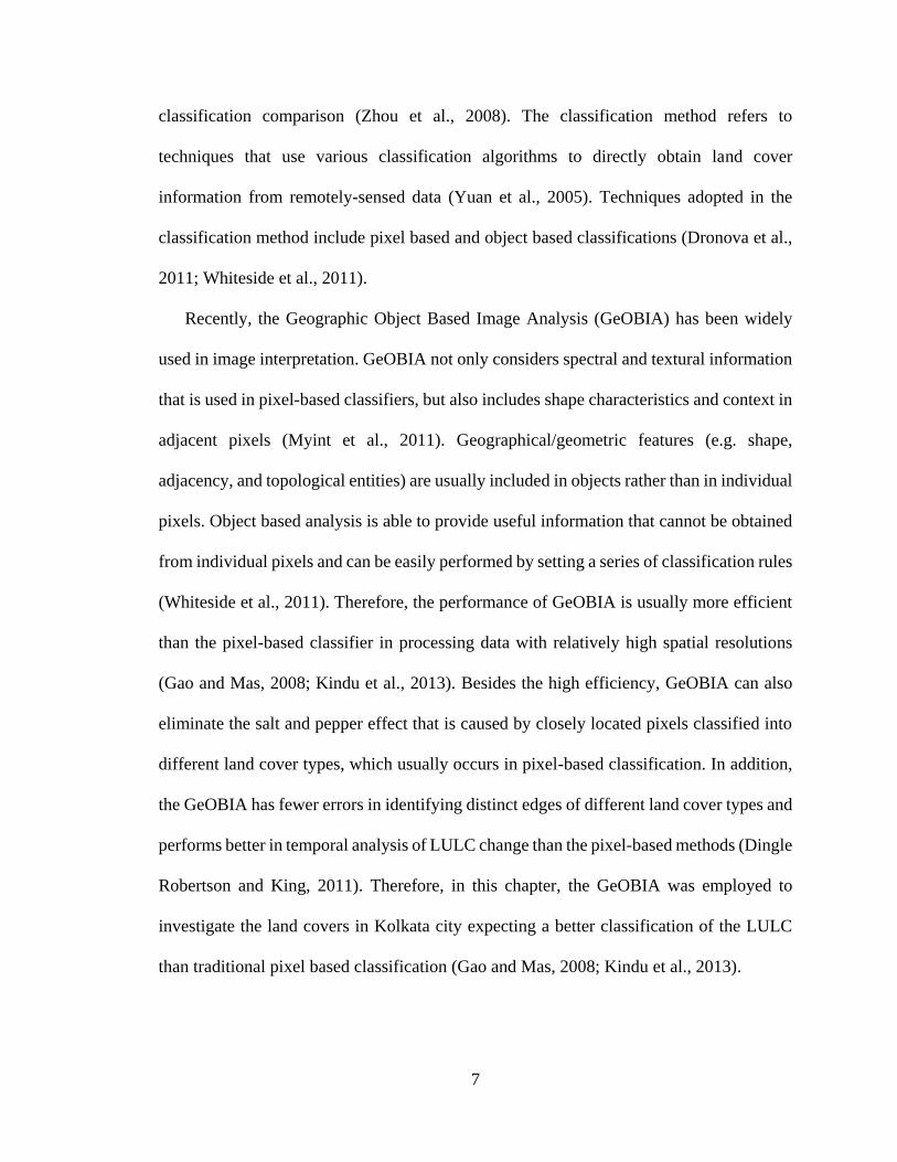
classification comparison (Zhou et al., 2008). The classification method refers to

techniques that use various classification algorithms to directly obtain land cover

information from remotely-sensed data (Yuan et al., 2005). Techniques adopted in the

classification method include pixel based and object based classifications (Dronova et al.,

2011; Whiteside et al., 2011).

Recently, the Geographic Object Based Image Analysis (GeOBIA) has been widely

used in image interpretation. GeOBIA not only considers spectral and textural information

that is used in pixel-based classifiers, but also includes shape characteristics and context in

adjacent pixels (Myint et al., 2011). Geographical/geometric features (e.g. shape,

adjacency, and topological entities) are usually included in objects rather than in individual

pixels. Object based analysis is able to provide useful information that cannot be obtained

from individual pixels and can be easily performed by setting a series of classification rules

(Whiteside et al., 2011). Therefore, the performance of GeOBIA is usually more efficient

than the pixel-based classifier in processing data with relatively high spatial resolutions

(Gao and Mas, 2008; Kindu et al., 2013). Besides the high efficiency, GeOBIA can also

eliminate the salt and pepper effect that is caused by closely located pixels classified into

different land cover types, which usually occurs in pixel-based classification. In addition,

the GeOBIA has fewer errors in identifying distinct edges of different land cover types and

performs better in temporal analysis of LULC change than the pixel-based methods (Dingle

Robertson and King, 2011). Therefore, in this chapter, the GeOBIA was employed to

investigate the land covers in Kolkata city expecting a better classification of the LULC

than traditional pixel based classification (Gao and Mas, 2008; Kindu et al., 2013).

8

Post-classification comparison provides land cover information by contrasting each

land cover class over time (Dewan and Yamaguchi, 2009) and thus has been widely used

for LULC change detection in various studies (Yuan et al., 2005; Zhou et al., 2008). An

advantage of this method is that it reduces change influences of using data provided by

multiple sensors under different atmospheric conditions or vegetation phenology stage

(Yuan et al., 2005; Zhou et al., 2008). A disadvantage is that this method is subject to error

propagation because the accuracy of post-classification comparison largely depends on the

accuracies of the individual classification for different time periods (Yuan et al., 2005;

Dewan and Yamaguchi, 2009). Therefore, high accuracy in image classification is a

prerequisite to produce reliable land cover change information.

In this chapter the GeOBIA method and post-classification comparison were applied to

detect land cover changes in Kolkata Metropolitan Development Area (KMDA) from 1990

to 2011. Objectives of this chapter were: 1) to investigate land cover changes in the KMDA

region using GeOBIA classification; 2) to analyze wetland conversion in recent years

through post-classification.

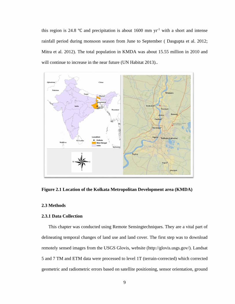
2.2 Study area

KMDA is the economic and cultural nucleus of eastern and north-eastern India. This

region is located in the eastern part of India with latitude ranging from 22°19' N to 23°01'

N and longitude from 88°04' E to 88°33' E. The total area of this region is approximate

1851 km2. It is one of the largest urban centers in Asia, and include the Kolkata Municipal

Corporation (KMC), 38 other municipalities, 77 non-municipal urban towns, 16 suburban

districts, and 445 rural districts (Dasgupta et al. 2012). The KMDA has a tropical climate

with a hot and humid summer and a dry and cool winter. The annual mean temperature of

9

this region is 24.8 ℃ and precipitation is about 1600 mm yr-1 with a short and intense

rainfall period during monsoon season from June to September ( Dasgupta et al. 2012;

Mitra et al. 2012). The total population in KMDA was about 15.55 million in 2010 and

will continue to increase in the near future (UN Habitat 2013)..

Figure 2.1 Location of the Kolkata Metropolitan Development area (KMDA)

2.3 Methods

2.3.1 Data Collection

This chapter was conducted using Remote Sensingtechniques. They are a vital part of

delineating temporal changes of land use and land cover. The first step was to download

remotely sensed images from the USGS Glovis, website (http://glovis.usgs.gov/). Landsat

5 and 7 TM and ETM data were processed to level 1T (terrain-corrected) which corrected

geometric and radiometric errors based on satellite positioning, sensor orientation, ground

10

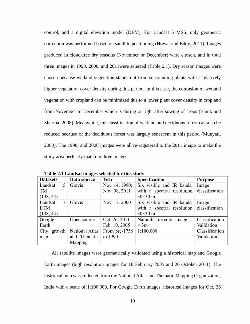
control, and a digital elevation model (DEM). For Landsat 5 MSS, only geometric

correction was performed based on satellite positioning (Howat and Eddy, 2011). Images

produced in cloud-free dry seasons (November or December) were chosen, and in total

three images in 1990, 2000, and 2011were selected (Table 2.1). Dry season images were

chosen because wetland vegetation stands out from surrounding plants with a relatively

higher vegetation cover density during this period. In this case, the confusion of wetland

vegetation with cropland can be minimized due to a lower plant cover density in cropland

from November to December which is during or right after sowing of crops (Banik and

Sharma, 2008). Meanwhile, misclassification of wetland and deciduous forest can also be

reduced because of the deciduous forest was largely senescent in this period (Munyati,

2000). The 1990, and 2000 images were all re-registered to the 2011 image to make the

study area perfectly match in three images.

Table 2.1 Landsat images selected for this study

Datasets Data source Year Specification Purpose

Landsat 5

TM

(138, 44)

Glovis Nov. 14, 1990;

Nov. 08, 2011

Six visible and IR bands,

with a spectral resolution

30×30 m

Image

classification

Landsat 7

ETM

(138, 44)

Glovis Nov. 17, 2000 Six visible and IR bands,


30×30 m

Image

classification

Google

Earth

Open source Oct. 26, 2011

Feb. 10, 2005

Natural/True color image,

< 3m

Classification

Validation

City growth

map

National Atlas

and Thematic

Mapping

From pre-1756

to 1990

1:100,000 Classification

Validation

All satellite images were geometrically validated using a historical map and Google

Earth images (high resolution images for 10 February 2005 and 26 October 2011). The

historical map was collected from the National Atlas and Thematic Mapping Organization,

India with a scale of 1:100,000. For Google Earth images, historical images for Oct. 26

11

2011 and Feb. 10, 2005 were used as references for data interpretation and classification

accuracy assessment of the Landsat images. Moreover, the classification results were also

compared with original Landsat images since there were few reference data for the study

area (Parihar et al., 2013).

2.3.2 LULC Classification

2.3.2.1 GeOBIA Classification

In this chapter, GeOBIA technique was to process the selected Landsat images. Four

land cover types were identified from the Landsat image data including wetlands with

water body only, wetlands with vegetation, built-up areas, and all other land cover types

(including forest, agriculture, and bare land). The GeOBIA method consists of two steps

including segmentation and rule-based classification (Zhou et al., 2008; Zohmann et al.,

2013). In segmentation, image data is divided into recognizable objects. Here a multi-

resolution segmentation with eCognition developer 8.64.0 software was used. The

segmentation algorithm is a bottom-up merging technique, beginning with a single pixel

and uses similarity rules to merge image data into larger units that is set by users (Zhou et

al., 2008; Kindu et al., 2013; Zohmann et al., 2013). Parameters used in this process include:

scale, shape, and compactness. The scale parameter is influenced by image heterogeneity

(considering object feature, color, and shape) and directly controls object sizes (Benz et al.,

2004). The greater the scale parameter is, the larger the average size of the objects that are

defined. Whiteside et al. (2011) emphasized the importance of scale parameter selection in

the GeOBIA classification. Large scale values may under-segment the image, leading to a

large number of mixed land covers; while small scale values could lead to over-segmenting

the image, causing high numbers of adjacent objects to be classified with the same land

12

cover. The shape parameter adjusts shape of objects using spectral values of image layers.

A maximum shape parameter of 1.0 suggests that created objects would not be related to

the spectral information, while with values less than 0.1 means the object is spectrally

homogeneous (Myint et al., 2011). According to Moffett and Gorelick (2013), wetland

features could be better distingushed using a low shape parameter. The compactness

parameter balances the compactness and smoothness of object boundaries. In this study,

the three parameters were estimated by visual interpretation to make sure most objects after

segmentation are internally homogenous (Zhou et al., 2008). Based on the trial and error

process, the scale parameters in this project were set to 3 for Landsat MSS image and 5 for

Landsat TM and ETM images with a shape parameter of 0.2 and a compactness parameter

of 0.7 for the two types of images, respectively

The rule-based classification used to define land cover class for each object

implemented the characteristics of brightness, size homogeneity, as well as Normalized

Difference Water Index (NDWI) and Normalized Difference Vegetation Index (NDVI)

(Gao, 1996; Zhou et al., 2008). NDWI was applied to separate water bodies from other

land cover types (Balçik, 2014). NDWI is a typical index in the multiple-band method used

to identify water surface from Landsat image data, as vegetation and open water show

distinctively different features of reflectance over the near infrared and green bands (Gao,

1996; Chen et al., 2006; Balçik, 2014). Similar to NDWI, NDVI is another widely used

multiple-band method to extract vegetation (including wetland vegetation, agricultural

plants and forests) from urban areas in this study. In the vegetation group, wetland

vegetation is distinguished from other land cover type because wetland vegetation has

higher NDVI values due to the low plant cover density in cropland from November to

13

December which is during or right after sowing of crops (Munyati, 2000; Banik & Sharma,

2008). Vegetation adjacent to a water body are most likely to be wetland vegetation

according to the wetland definition (Cedfeldt et al., 2000; Wright and Gallant, 2007).

Therefore, besides NDVI, distance to water was also used as a rule for wetland vegetation

classification in processing satellite data. Brightness and size homogeneity were also

applied to further separate built-up areas and other land cover types (Salehi et al., 2012).

Four images were classified with similar rulesets but different threshold values for all

classes.

2.3.2.2 Accuracy Assessment

The eCognition software provides four accuracy assessment methods including

classification stability, best classification result, error matrix based on Test and Training

Area (TTA) mask, and error matrix based on sample. According to eCognition 8.64.0 user

guide (http://www.ecognition.cc/download/eCognition_8.64.0_Release_Notes.pdf), the

classification stability computes the difference between the largest and the second largest

membership values for each pixel and sums for the whole class. The best classification

result shows a visual representation of the pixel with the largest membership value. The

error matrix based on TTA mask uses test areas as reference data to check results of

classification. The error matrix based on sample is similar to error matrix based on TTA

mask, but it considers samples not pixels of a TTA mask. In this study, the error matrix

based on TTA mask was chosen as the assessment method, which is commonly used for

accuracy evaluation in remote sensing data classification (Zohmann et al., 2013). A TTA

mask with 200 test objects was created for each image and verified using the historical map,

the Google Earth images and the classified images by previous studies. Then the masks

were loaded in eCognition software to compare if the classes in the classified images are

14

in agreement with the test areas in the mask. After comparison, the overall accuracy,

producer’s accuracy, and user’s accuracy were provided by the error matrix and the

percentage of objects that was correctly identified for each class can be obtained. The

producer’s accuracy shows the omission errors related to a class. It is derived from the

number of correctly classified pixels of a class divided by the total number of pixels of that

class used for assessment. The user’s accuracy measures the commission errors related to

a class. It is calculated by the number of pixels correctly classified divided by the total

number of pixels predicted to be that class in the assessment (Foody, 2005).

2.3.3 Post-classification Comparison Change Detection

Post-classification is a commonly used method to validate and compare the rate of

change of LULC. Here it was applied to investigate change of LULC from 1990 to 2011

in the study area. Based on the classified images, two periods were compared to

demonstrate LULC changes with time, including 1990-2000 and 2000-2011. For each

period, a matrix process was used to compare two classified vector images using ERDAS

software. Using the classified images as input files and selecting a default 1 meter as the

output cell size, the two vector images were converted to a raster image with changing

areas in the attribute table to present land cover changes. Land conversion was quantified

by comparing the area value of one class with the corresponding value of that class in the

other image. This value is expressed as a percentage of LULC changes (P, %) (Eq.1)

(Kindu et al., 2013) and quantified as a conversion rate (r) (Eq.2):

𝑃𝑖 = (𝐴𝑖,𝑓𝑖𝑛𝑎𝑙−𝐴𝑖,𝑖𝑛𝑖𝑡𝑖𝑎𝑙

𝐴𝑖,𝑖𝑛𝑖𝑡𝑖𝑎𝑙) × 100 (Eq.1)

𝑟𝑖 = (𝐴𝑖,𝑓𝑖𝑛𝑎𝑙−𝐴𝑖,𝑖𝑛𝑖𝑡𝑖𝑎𝑙

𝛥𝑦𝑒𝑎𝑟) × 100 (Eq.2)

15

where i refers to the ith class of land cover for change detection, Ainitial and Afinal are the

areas of class in the initial year and in the final year, respectively, 𝛥year represents the total

years between the initial year and the final year. For P and r, positive values suggest an

increasing area of that land cover class during study period, while negative values suggest

a decreasing land cover area with time.

2.4 Result and discussion

2.4.1 Accuracy Assessment

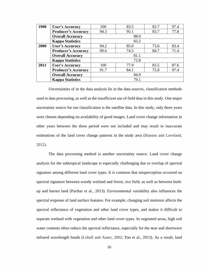
Accuracy assessment of the classification results was conducted by checking the

user’s accuracy and producer’s accuracy for each land cover types, as well as overall

accuracy and kappa statistics for the each classified land cover maps. In general, the

GeOBIA classification provides reasonable land cover information for the study area since

the overall accuracy of the satellite image interpretation ranged from 81.1% to 88.0%. Of

all the four land cover types, wetlands with water bodies had the highest accuracy. Both

the user’s and the producer’s accuracies for this land cover type were over 90%. For the

built-up area, the accuracy analysis showed comparable producer’s and user’s accuracy in

1990. The user’s accuracy was lower than that of producer’s in 2000 but higher in 2011.

For the wetlands with vegetation, the producer’s accuracy was higher (95.1%) in 1990 than

the other years. For the other years, both producer’s and user’s accuracies ranged from

74.5% to 85%. Highest user’s accuracy occurred in 1990, whereas the highest producer’s

accuracy occurred in 2011.

Table 2.2 Summaries of classification accuracies (%) for Landsat images of 1990,

2000, and 2011

Water

(wetlands)

Vegetation

(Wetlands)

Built-up

areas

Others

16

1990 User’s Accuracy 100 83.5 83.7 97.4

Producer’s Accuracy 94.3 95.1 83.7 77.8

Overall Accuracy 88.0

Kappa Statistics 83.2

2000 User’s Accuracy 94.2 85.0 73.6 83.4




2011 User’s Accuracy 100 77.9 83.5 87.6




Uncertainties of in the data analysis lie in the data sources, classification methods

used in data processing, as well as the insufficient use of field data in this study. One major

uncertainty source for our classification is the satellite data. In this study, only three years

were chosen depending on availability of good images. Land cover change information in

other years between the three period were not included and may result in inaccurate

estimations of the land cover change patterns in the study area (Hansen and Loveland,

2012).

The data processing method is another uncertainty source. Land cover change

analysis for the subtropical landscape is especially challenging due to overlap of spectral

signature among different land cover types. It is common that misperception occurred on

spectral signature between woody wetland and forest, rice field, as well as between built-

up and barren land (Parihar et al., 2013). Environmental variability also influences the

spectral response of land surface features. For example, changing soil moisture affects the

spectral reflectance of vegetation and other land cover types, and makes it difficult to

separate wetland with vegetation and other land cover types. In vegetated areas, high soil

water contents often reduce the spectral reflectance, especially for the near and shortwave

infrared wavelength bands (Lobell and Asner, 2002; Pan et al., 2013). As a result, land

17

cover classification based on pure spectral signatures in the wetland environment may

result in poor classification performance. In addition, more ground truth activities should

be performed to improve the land cover classification and for the evaluation of

classification results.

2.4.2 Land cover changes in KMDA

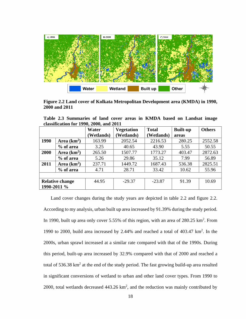
Spatial distributions of major land covers in the study area can be found in the

classification results of the satellite images (Figure 2.2). Wetlands and the other category

land cover are the two major land cover types. Percentages of total wetlands were 43.90%,

35.12% and 33.42% in 1990, 2000 and 2011 respectively. Wetlands with surface waters

were mainly distributed along the Hooghly River, and the southeastern areas in this region.

In 2000, surface waters also appeared in southwest parts of this region. Areas along the

river channel are also regions where vegetated wetland area are located. Large areas of

vegetated wetland were mainly located in the southern parts of the study area in 1990. In

eastern parts of this region, vegetated wetlands were mainly scattered among other land

cover types. In 2000, vegetated wetland areas in the south parts were reduced significantly,

and the reduction trend continued in 2011. Built-up regions were mainly distributed along

the river, especially around the Kolkata city. Locations of area with large built-up regions

remained unchanged in the study area but size of the built-up regions increased, especially

in south and southeast Kolkata. In addition, built-up areas spread out and scattered over

much larger regions in 2011 than the other two years.

18

Figure 2.2 Land cover of Kolkata Metropolitan Development area (KMDA) in 1990,

2000 and 2011

Table 2.3 Summaries of land cover areas in KMDA based on Landsat image

classification for 1990, 2000, and 2011

Water

(Wetlands)

Vegetation

(Wetlands)

Total

(Wetlands)

Built-up

areas

Others

1990 Area (km2) 163.99 2052.54 2216.53 280.25 2552.58

% of area 3.25 40.65 43.90 5.55 50.55

2000 Area (km2) 265.50 1507.77 1773.27 403.47 2872.63

% of area 5.26 29.86 35.12 7.99 56.89

2011 Area (km2) 237.71 1449.72 1687.43 536.38 2825.51

% of area 4.71 28.71 33.42 10.62 55.96

Relative change

1990-2011 %

44.95 -29.37 -23.87 91.39 10.69

Land cover changes during the study years are depicted in table 2.2 and figure 2.2.

According to my analysis, urban built up area increased by 91.39% during the study period.

In 1990, built up area only cover 5.55% of this region, with an area of 280.25 km2. From

1990 to 2000, build area increased by 2.44% and reached a total of 403.47 km2. In the

2000s, urban sprawl increased at a similar rate compared with that of the 1990s. During

this period, built-up area increased by 32.9% compared with that of 2000 and reached a

total of 536.38 km2 at the end of the study period. The fast growing build-up area resulted

in significant conversions of wetland to urban and other land cover types. From 1990 to

2000, total wetlands decreased 443.26 km2, and the reduction was mainly contributed by

19

wetlands with vegetation, which decreased by 544.77 km2, whereas wetlands with water

bodies increased by 101.51 km2 during the same period. The increased water body may be

caused by a high precipitation rate at this region in 2000, which increased areas of wetlands

and water bodies of temperate wetlands (Rao et al., 2004). For the second period, total

wetland areas further decreased, but at a much slower rate. The period from 2000 to 2011

witnessed a decrease of 85.84 km2 in total wetland areas, and this reduction was attributable

to both wetlands with vegetation and surface waters. Besides built-up areas and wetlands,

other land cover types identified in this study also showed significant changes, especially

for the 1990s. During 1990 and 2000, this land cover category increased by 320.05 km2.

However, in the second period (2000-2011), total area of this category did not show

significant changes.2.4.3 Land conversions among major land cover types in KMDA

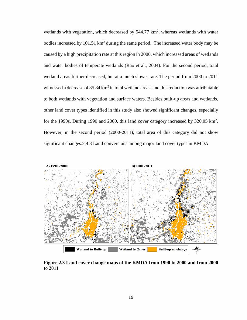
Figure 2.3 Land cover change maps of the KMDA from 1990 to 2000 and from 2000

to 2011

20

Figure 2.3 demonstrates land cover conventions in the two time periods. From 1990 to

2000, urban area in the central regions of the study area has increased dramatically. Urban

sprawl also occurred in the southern edges of the Kolkata city. During this period, land

conversion from wetlands to other land cover types mainly scattered in the southern parts

of the study area, especially in the southwest parts. Land conversions between 2000 and

2011 from wetland to urban area were significant. In this period, the results showed large

areas of wetland conversion along the Hooghly River channels in the northern regions of

the Kolkata city. Meanwhile, there were also large areas of wetlands converted to other

land cover types and the conversion mainly occurred along the Hooghly River, in

southwestern and northeastern areas of this region.

Natural properties and human activities are two major groups of drivers accounting

for land cover change (Veldkamp and Fresco 1996). Specifically, natural properties refer

to physical and chemical conditions of soil, climate factors, as well as pest and disease

impacts, whereas human factors reference to population increase and economic activities.

For the KMDA area, natural and anthropogenic factors both resulted in land cover changes.

For example, wetland ecosystems are sensitive to amount of water supply (Erwin, 2009).

During low precipitation periods, some temperate wetlands may dry up or even be used as

croplands (Parihar et al., 2013). This shows a natural factor influencing land cover types.

Population growth is another major reason for the urban sprawl. UN habitat (2013) showed

that population increased by 50% from 1990 to 2011 in this area. As presented in previous

sections, increasing urban areas were mainly distributed in areas adjacent to the Kolkata

area. Expanding population requires extra supply of food, facilities for housing as well as

infrastructures for transportation and commercial activities. As a result, wetlands or other

21

land cover types in the adjacent regions of the Kolkata city were removed and cleared for

construction. Increasing populations also required more agricultural products which led to

expansion of other land cover types from 1990 to 2000.

22

2.5 Reference

Balçik, F. B. (2014). Determining the impact of urban components on land surface

temperature of Istanbul by using remote sensing indices. Environmental Monitoring

and Assessment, 186(2), 859–872. doi:10.1007/s10661-013-3427-5

Banik, P., & Sharma, R. C. (2008). Effects of integrated nutrient management with

mulching on rice (Oryza sativa) – based cropping systems in rainfed eastern plateau

area. Indian Journal of Agricultural Sciences, 78, 243–3.

Benz, U. C., Hofmann, P., Willhauck, G., Lingenfelder, I., & Heynen, M. (2004). Multi-

resolution, object-oriented fuzzy analysis of remote sensing data for GIS-ready

information. ISPRS Journal of Photogrammetry and Remote Sensing, 58(3-4), 239–

258. doi:10.1016/j.isprsjprs.2003.10.002

Cedfeldt, P. T., Watzin, M. C., & Richardson, B. D. (2000). Using GIS to identify

functionally significant wetlands in the northeastern United States. Environmental

Management, 26(1), 13–24. doi:10.1007/s002670010067

Chen, X.-L., Zhao, H.-M., Li, P.-X., & Yin, Z.-Y. (2006). Remote sensing image – based

analysis of the relationship between urban heat island and land use/cover changes.

Remote Sensing of Environment, 104(2), 133–146. doi:10.1016/j.rse.2005.11.016

Dasgupta, S., Gosain, A. K., Rao, S., Roy, S., & Sarraf, M. (2013). A megacity in a

changing climate: the case of Kolkata. Climatic change, 116(3-4), 747-766.

Dewan, A. M., & Yamaguchi, Y. (2009). Land use and land cover change in Greater

Dhaka, Bangladesh: Using remote sensing to promote sustainable urbanization.

Applied Geography, 29(3), 390–401. doi:10.1016/j.apgeog.2008.12.005

Dingle Robertson, L., & King, D. J. (2011). Comparison of pixel- and object-based

classification in land cover change mapping. International Journal of Remote Sensing,

32(6), 1505–1529. doi:10.1080/01431160903571791

Dronova, I., Gong, P., & Wang, L. (2011). Object-based analysis and change detection of

major wetland cover types and their classification uncertainty during the low water

period at Poyang Lake, China. Remote Sensing of Environment, 115(12), 3220–3236.

doi:10.1016/j.rse.2011.07.006

Erwin, K. L. (2009). Wetlands and global climate change: the role of wetland restoration

in a changing world. Wetlands Ecology and management, 17(1), 71-84.

Foody, G. M. (2005). Local characterization of thematic classification accuracy through

spatially constrained confusion matrices. International Journal of Remote

Sensing, 26(6), 1217-1228.

23

Gao, B. (1996). NDWI – a normalized difference water index for remote sensing of

vegetation liquid water from space. Remote Sensing of Environment, 58, 257–266.

Gao, Y., & Mas, J. F. (2008). A comparison of the performance of pixel based and object

based classifications over images with various spatial resolutions. OnLine Journal of

Earth Sciences, 2(1), 27–35.

Hansen, M. C., & Loveland, T. R. (2012). A review of large area monitoring of land cover

change using Landsat data. Remote sensing of Environment, 122, 66-74.

Howat, I. M., & Eddy, A. (2011). Multi-decadal retreat of Greenland’s marine-terminating

glaciers. Journal of Glaciology, 57, 389–396.

Karar, K., & Gupta, A. K. (2006). Seasonal variations and chemical characterization of

ambient PM10 at residential and industrial sites of an urban region of Kolkata

(Calcutta), India. Atmospheric Research, 81(1), 36–53.

doi:10.1016/j.atmosres.2005.11.003

Kindu, M., Schneider, T., Teketay, D., & Knoke, T. (2013). Land use/Land cover change

analysis using object-based classification approach in Munessa-Shashemene

landscape of the Ethiopian Highlands. Remote Sensing, 5(5), 2411–2435.

doi:10.3390/rs5052411

Lobell, D. B., & Asner, G. P. (2002). Moisture effects on soil reflectance. Soil Science

Society of America Journal, 66(3), 722-727.

Moffett, K. B., & Gorelick, S. M. (2013). Distinguishing wetland vegetation and channel

features with object-based image segmentation. International Journal of Remote

Sensing, 34(4), 1332–1354. doi:10.1080/01431161.2012.718463

Munyati, C. (2000). Wetland change detection on the Kafue Flats, Zambia, by

classification of a multitemporal remote sensing image dataset. International Journal

of Remote Sensing, 21(9), 1787–1806.

Myint, S. W., Gober, P., Brazel, A., Grossman-Clarke, S., & Weng, Q. (2011). Per-pixel

vs. object-based classification of urban land cover extraction using high spatial

resolution imagery. Remote Sensing of Environment, 115(5), 1145–1161.

doi:10.1016/j.rse.2010.12.017

Pan, S., Li, G., Yang, Q., Ouyang, Z., Lockaby, G., & Tian, H. (2013). Monitoring Land-

Use and Land-Cover Change in the Eastern Gulf Coastal Plain 3 using Multi-temporal

Landsat imagery. Journal of Geophysics & Remote Sensing.


wetland dynamics a post-classification change detection analysis of the East Kolkata

Wetlands using open source satellite data. Geocarto International, 28(3), 273–287.

24

Rao, G. P., Jaswal, A. K., & Kumar, M. S. (2004). Effects of urbanization on

meteorological parameters. Mausam, 55(3), 429-440

Salehi, B., Zhang, Y., Zhong, M., & Dey, V. (2012). Object-based classification of urban

areas using VHR imagery and height points ancillary data. Remote Sensing, 4(12),

2256–2276. doi:10.3390/rs4082256

Sharma, R., Chakraborty, A., & Joshi, P. K. (2015). Geospatial quantification and analysis

of environmental changes in urbanizing city of Kolkata (India).Environmental

monitoring and assessment, 187(1), 1-12.

Taubenböck, H., Wegmann, M., Roth, a., Mehl, H., & Dech, S. (2009). Urbanization in

India – Spatiotemporal analysis using remote sensing data. Computers, Environment

and Urban Systems, 33(3), 179–188. doi:10.1016/j.compenvurbsys.2008.09.003

UN (2012). World urbanization prospects – The 2011 revision. New York: United Nation

Department of Economic and Social Affairs/Population Division.

UN Habitat. (2013). State of the world’s cities 2012/2013: Prosperity of cities (p. 135).

Washington, DC.

Veldkamp A and Fresco L O 1996 CLUE : a conceptual model to study the Conversion of

Land Use and its Effects Ecological Modelling 85 253–70

Whiteside, T. G., Boggs, G. S., & Maier, S. W. (2011). Comparing object-based and pixel-

based classifications for mapping savannas. International Journal of Applied Earth

Observation and Geoinformation, 13(6), 884–893. doi:10.1016/j.jag.2011.06.008

Wright, C., & Gallant, A. (2007). Improved wetland remote sensing in Yellowstone

National Park using classification trees to combine TM imagery and ancillary

environmental data. Remote Sensing of Environment, 107(4), 582–605.

doi:10.1016/j.rse.2006.10.019

Yuan, F., Sawaya, K. E., Loeffelholz, B. C., & Bauer, M. E. (2005). Land cover

classification and change analysis of the Twin Cities (Minnesota) Metropolitan Area

by multitemporal Landsat remote sensing. Remote Sensing of Environment, 98(2-3),

317–328. doi:10.1016/j.rse.2005.08.006

Zhou, W., Troy, A. & Grove, M., 2008. Object-based Land Cover Classification and

Change Analysis in the Baltimore Metropolitan Area Using Multitemporal High

Resolution Remote Sensing Data. Sensors, 8, pp.1613–1636.

Zohmann, M., Pennerstorfer, J., & Nopp-Mayr, U. (2013). Modelling habitat suitability for

alpine rock ptarmigan (Lagopus muta helvetica) combining object-based

classification of IKONOS imagery and Habitat Suitability Index modelling.

Ecological Modelling, 254, 22–32. doi:10.1016/j.ecolmodel.2013.01.008

25

26

3. Spatial and Temporal Patterns of Wetland Cover changes in

East Kolkata, India from 1972 to 20111

1 This chapter has been accepted by Journal of Applied Geospatial Research. (Li, X., Mitra, C.,

Marzen, L., & Yang, Q. (2015). Spatial and Temporal Patterns of Wetland Cover changes in East

Kolkata Wetlands, India from 1972 to 2011. International Journal of Applied Geospatial Research

(Accepted).)

3.1 Introduction

Wetland ecosystems are transitional regions between terrestrial and aquatic ecosystems

with unique soil conditions, plants, and animals, and are essential components of terrestrial

carbon and nutrient cycles (Mitsch and Gosselink, 2007; Cui et al., 2009; Li et al., 2012).

Initially, conversion of wetland areas to agricultural lands was a main reason for wetland

loss globally. Large areas wetlands were converted to cropland to sustain food production

for the ever-increasing population (Rijsberman and De Silva, 2003). In recent time

population growth and urbanization have further undermined wetland areas and gradually

converted them to built-up areas and agricultural lands (Bolca et al., 2007; Cui et al., 2010;

Parihar et al., 2013). Drainage ditches for cropland have significantly lowered the water

table depth of wetlands and reduced water-storage capacity and changed local hydrological

cycling such as precipitation and runoff (Bartzen et al., 2010). Wetland conversion to built-

up area results in an increase in impervious surfaces which may cause increases in

evapotranspiration and runoff (Carlson and Arthur, 2000). These changes may also

increase temperature due to rising greenhouse gas emissions from human-related sources

and reduced vegetation covers (Chen et al., 2006; Balçik, 2014). Therefore, a thorough

27

investigation of LULC dynamics on wetland ecosystems is the key to understandings of

LULC change-induced hydrological, ecological and climatic processes.

The geographic object-based analysis is being widely used for wetland classification in

recent years (Dingle Robertson and King, 2011; Dronova et al., 2011; Moffett and Gorelick,

2013). As introduced in Chapter 2, it can reduce the salt and pepper effect and has fewer

edge errors compared with the pixel-based methods. Since high spectral and spatial

heterogeneities exist in wetland classification due to differences in water depths and

vegetation, the process is highly context-dependent (Wright and Gallant, 2007; Cui et al.,

2010). The features of object-based analysis make GeOBIA a very useful method in

investigating changes in wetlands over long periods. Identifying related indices is the key

for wetland detection during the classification process. Water body is a commonly used

index to identify wetlands in satellite images (Mitsch and Gosselink, 2007). Surface water

shows relatively higher reflectance in the visible wavelengths and lower reflectance in

near-infrared wavelengths than other land cover types, so it can be extracted through a

multi-band technique which considers the reflectance of water over multiple bands (Jensen,

2006; Campbell and Wynne, 2011). The Normalized Difference Water Index (NDWI) is a

typical index in the multiple-band method used to identify water surface from Landsat

image data, as vegetation and open water show distinctively different features of

reflectance over the near infrared and green bands (Gao, 1996; Chen et al., 2006; Balçik,

2014). Moreover, Munyati (2000) used dry season Landsat images to distinguish wetland

vegetation from deciduous forest since wetland vegetation shown a higher Normalized

Difference Vegetation Index (NDVI) than deciduous forest that was largely senescent in

autumn.

28

In this chapter, the GeoBIA and post-classification comparison were applied to detect

wetland shrinkage in East Kolkata Wetlands (EKWs), India, from 1972 to 2011. EKWs are

important to Kolkata, eastern India because they have reduced soil erosion and act as water

receivers and nutrient purifiers (Bhatta, 2009; Parihar et al., 2013). In 2002, the EKWs

were designated as “Wetland of International Importance” under the Ramsar Convention.

However, due to the rapid population growth, large areas of wetlands have been converted

to agricultural and built-up areas, especially for vegetated areas of wetlands which are more

susceptible to human disturbances and can be easily transformed to croplands and built-up

areas (Hartig et al., 1997; Bartzen et al., 2010; Parihar et al., 2013). The substantial decrease

in wetlands has raised increasing concerns and also helped etch out the research question

for our study - How EKWs land cover has changed over time? Though Parihar et al. (2013)

have studied open water area shrinkage in EKWs using a traditional pixel-based

classification, they paid little attention about the vegetation areas of wetlands. In this study,

the GeOBIA was applied in an attempt to accomplish a more detailed wetland classification

of EKWs considering both water bodies and wetland vegetation. The objectives of this

study were: 1) to classify LULC in EKW region using GeOBIA classification; 2) to analyze

and quantify LULC dynamics during the study period; 3) to discuss spatial patterns of

wetland conversion. Results of the study provide useful information on the historical LULC

changes which can be used to assess impacts of land conversions on regional hydrology,

biodiversity and climate in Kolkata city which experience intensive urbanization and

agricultural expansion.

3.2 Study Area

29

Figure 3.1 Location of the East Kolkata Wetlands (EKWs)

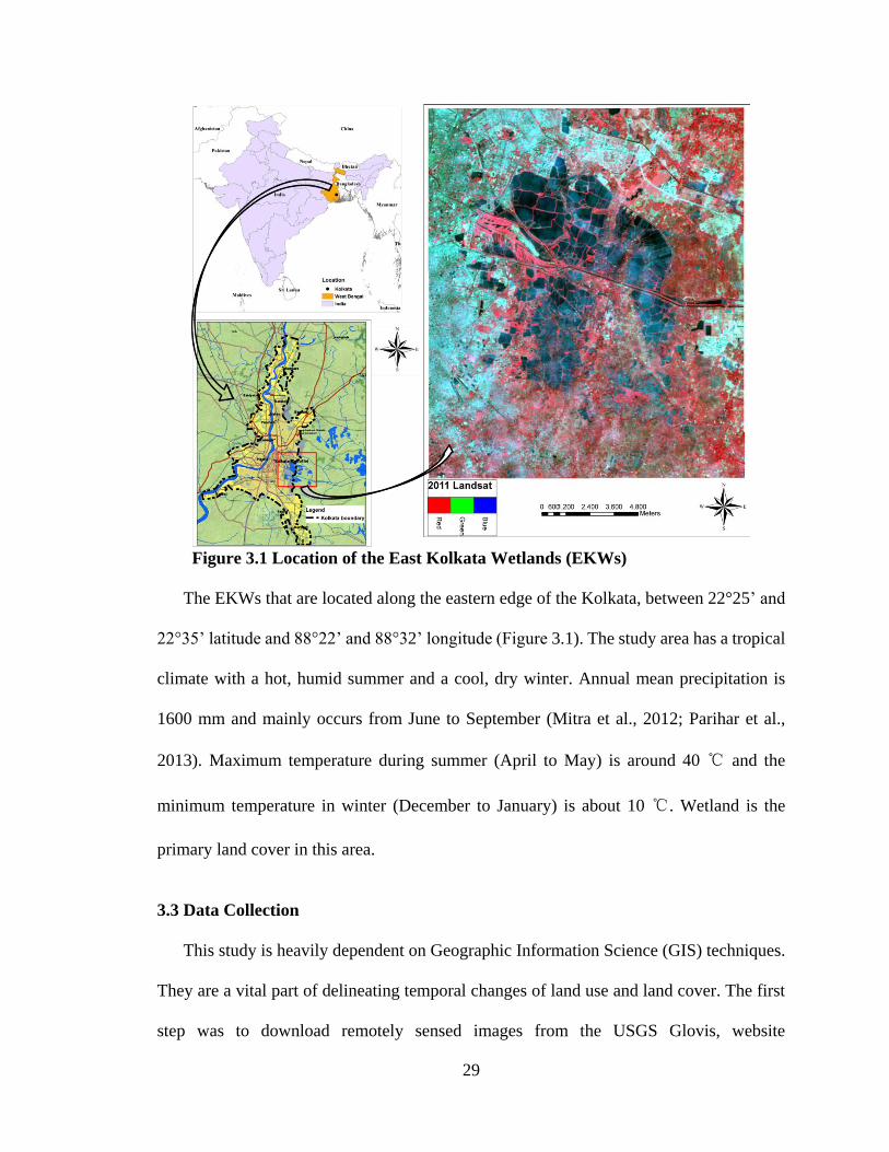
The EKWs that are located along the eastern edge of the Kolkata, between 22°25’ and

22°35’ latitude and 88°22’ and 88°32’ longitude (Figure 3.1). The study area has a tropical

climate with a hot, humid summer and a cool, dry winter. Annual mean precipitation is

1600 mm and mainly occurs from June to September (Mitra et al., 2012; Parihar et al.,

2013). Maximum temperature during summer (April to May) is around 40 ℃ and the

minimum temperature in winter (December to January) is about 10 ℃. Wetland is the

primary land cover in this area.

3.3 Data Collection

This study is heavily dependent on Geographic Information Science (GIS) techniques.

They are a vital part of delineating temporal changes of land use and land cover. The first

step was to download remotely sensed images from the USGS Glovis, website

30

(http://glovis.usgs.gov/). Landsat 5 and 7 TM and ETM data were processed to level 1T

(terrain-corrected) which corrected geometric and radiometric errors based on satellite

positioning, sensor orientation, ground control, and a digital elevation model (DEM). For

Landsat 1-5 MSS, only geometric correction was applied based on satellite positioning

(Howat and Eddy, 2011). Images generated in cloud-free dry seasons (November or

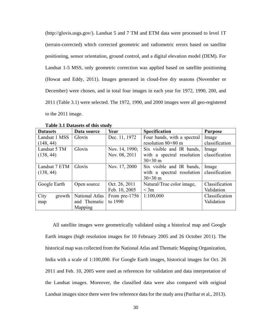
December) were chosen, and in total four images in each year for 1972, 1990, 200, and

2011 (Table 3.1) were selected. The 1972, 1990, and 2000 images were all geo-registered

to the 2011 image.

Table 3.1 Datasets of this study

Datasets Data source Year Specification Purpose

Landsat 1 MSS

(148, 44)

Glovis Dec. 11, 1972 Four bands, with a spectral

resolution 80×80 m

Image

classification

Landsat 5 TM

(138, 44)

Glovis Nov. 14, 1990;

Nov. 08, 2011

Six visible and IR bands,


30×30 m

Image

classification

Landsat 7 ETM

(138, 44)

Glovis Nov. 17, 2000 Six visible and IR bands,


30×30 m

Image

classification

Google Earth Open source Oct. 26, 2011

Feb. 10, 2005

Natural/True color image,

< 3m

Classification

Validation

City growth

map

National Atlas

and Thematic

Mapping

From pre-1756

to 1990

1:100,000 Classification

Validation

All satellite images were geometrically validated using a historical map and Google

Earth images (high resolution images for 10 February 2005 and 26 October 2011). The

historical map was collected from the National Atlas and Thematic Mapping Organization,

India with a scale of 1:100,000. For Google Earth images, historical images for Oct. 26

2011 and Feb. 10, 2005 were used as references for validation and data interpretation of

the Landsat images. Moreover, the classified data were also compared with original

Landsat images since there were few reference data for the study area (Parihar et al., 2013).

31

After LULC change analysis, population data in Kolkata city were also collected to

further investigate if the population growth of Kolkata city could be a cause for possible

wetland conversions. The population data were collected from studies of United Nations

(2005) and UN Habitat (2013) and were linearly interpolated to generate population data

in 1972, 1990, 2000, and 2011.

3.4 Results and Discussion

3.4.1 Wetland Shrinkage and Built-up Area Expansion

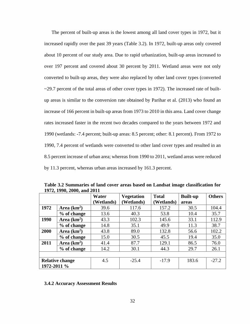
Wetlands (including open water and wetlands with vegetation) were the major land

cover type in study area, accounting for 53.9 percent of the total region in 1972 (Table 3.2).

From 1972 to 2011, total wetland areas decreased by 28.1 km2, leading to a 17.9 percent

reduction. Open water area showed relatively low variability among the four study years

(ranging from 39.6 km2 to 43.8 km2) and was about 5 percent smaller in 1972 than other

years; while vegetation zones of wetlands decreased about 30.0 km2 during the 39 years,

accounting for 25.4 percent of the total region in 1972. This result is reasonable because

open water area can also be influenced by precipitation. Low monsoonal rainfall was found

in EKWs during 1972 (Mitra et al., 2012), which might reduce areas with surface water in

some seasonal wetlands and wetlands with low water depth. For the vegetation zones, since

most land is arable with a lower water depth than in open water, they were vulnerable to

human activities and were readily used for urban construction and agricultural development

(Yuan et al., 2005; Biswas, 2010). The results further suggest that wetlands cannot be

effectively classified if water bodies are used as the only indicator. This may be one reason

for the low accuracies in wetland classification in the study by Parihar et al. (2013).

32

The percent of built-up areas is the lowest among all land cover types in 1972, but it

increased rapidly over the past 39 years (Table 3.2). In 1972, built-up areas only covered

about 10 percent of our study area. Due to rapid urbanization, built-up areas increased to

over 197 percent and covered about 30 percent by 2011. Wetland areas were not only

converted to built-up areas, they were also replaced by other land cover types (converted

~29.7 percent of the total areas of other cover types in 1972). The increased rate of built-

up areas is similar to the conversion rate obtained by Parihar et al. (2013) who found an

increase of 166 percent in built-up areas from 1973 to 2010 in this area. Land cover change

rates increased faster in the recent two decades compared to the years between 1972 and

1990 (wetlands: -7.4 percent; built-up areas: 8.5 percent; other: 8.1 percent). From 1972 to

1990, 7.4 percent of wetlands were converted to other land cover types and resulted in an

8.5 percent increase of urban area; whereas from 1990 to 2011, wetland areas were reduced

by 11.3 percent, whereas urban areas increased by 161.3 percent.

Table 3.2 Summaries of land cover areas based on Landsat image classification for

1972, 1990, 2000, and 2011

Water

(Wetlands)

Vegetation

(Wetlands)

Total

(Wetlands)

Built-up

areas

Others

1972 Area (km2) 39.6 117.6 157.2 30.5 104.4

% of change 13.6 40.3 53.8 10.4 35.7

1990 Area (km2) 43.3 102.3 145.6 33.1 112.9

% of change 14.8 35.1 49.9 11.3 38.7

2000 Area (km2) 43.8 89.0 132.8 56.6 102.2

% of change 15.0 30.5 45.5 19.4 35.0

2011 Area (km2) 41.4 87.7 129.1 86.5 76.0

% of change 14.2 30.1 44.3 29.7 26.1

Relative change

1972-2011 %

4.5 -25.4 -17.9 183.6 -27.2

3.4.2 Accuracy Assessment Results

33

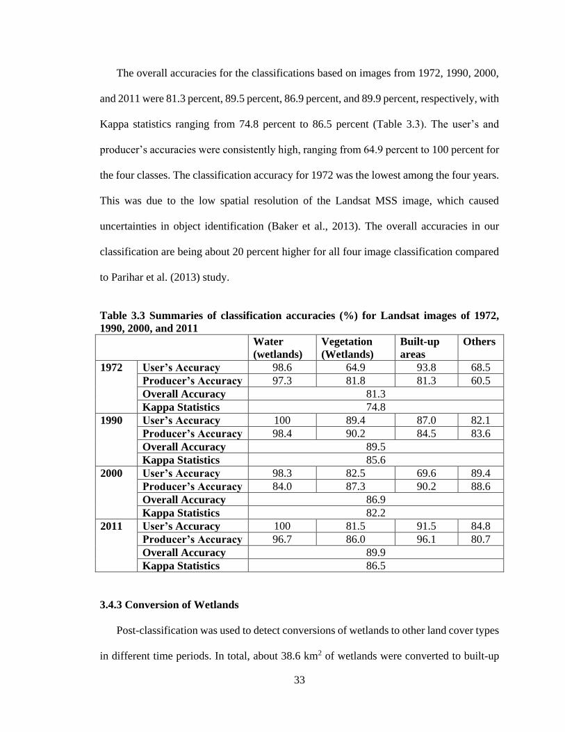
The overall accuracies for the classifications based on images from 1972, 1990, 2000,

and 2011 were 81.3 percent, 89.5 percent, 86.9 percent, and 89.9 percent, respectively, with

Kappa statistics ranging from 74.8 percent to 86.5 percent (Table 3.3). The user’s and

producer’s accuracies were consistently high, ranging from 64.9 percent to 100 percent for

the four classes. The classification accuracy for 1972 was the lowest among the four years.

This was due to the low spatial resolution of the Landsat MSS image, which caused

uncertainties in object identification (Baker et al., 2013). The overall accuracies in our

classification are being about 20 percent higher for all four image classification compared

to Parihar et al. (2013) study.

Table 3.3 Summaries of classification accuracies (%) for Landsat images of 1972,

1990, 2000, and 2011

Water

(wetlands)

Vegetation

(Wetlands)

Built-up

areas

Others

1972 User’s Accuracy 98.6 64.9 93.8 68.5




1990 User’s Accuracy 100 89.4 87.0 82.1




2000 User’s Accuracy 98.3 82.5 69.6 89.4




2011 User’s Accuracy 100 81.5 91.5 84.8




3.4.3 Conversion of Wetlands

Post-classification was used to detect conversions of wetlands to other land cover types

in different time periods. In total, about 38.6 km2 of wetlands were converted to built-up

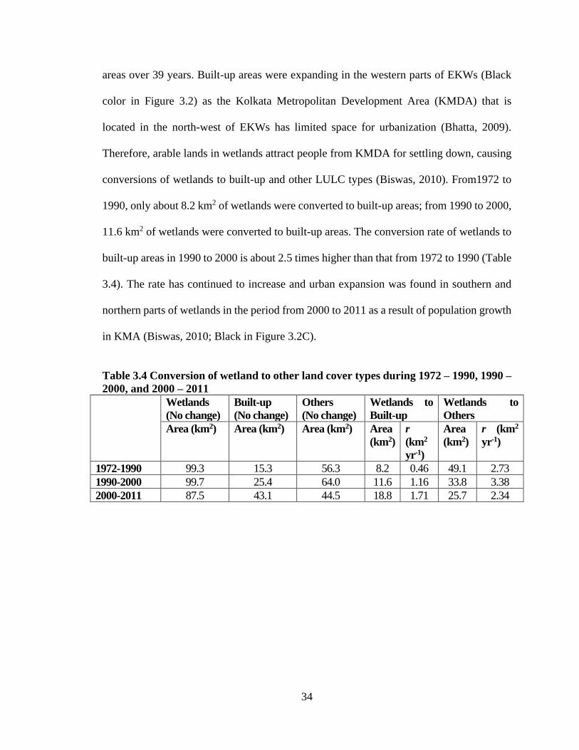
34

areas over 39 years. Built-up areas were expanding in the western parts of EKWs (Black

color in Figure 3.2) as the Kolkata Metropolitan Development Area (KMDA) that is

located in the north-west of EKWs has limited space for urbanization (Bhatta, 2009).

Therefore, arable lands in wetlands attract people from KMDA for settling down, causing

conversions of wetlands to built-up and other LULC types (Biswas, 2010). From1972 to

1990, only about 8.2 km2 of wetlands were converted to built-up areas; from 1990 to 2000,

11.6 km2 of wetlands were converted to built-up areas. The conversion rate of wetlands to

built-up areas in 1990 to 2000 is about 2.5 times higher than that from 1972 to 1990 (Table

3.4). The rate has continued to increase and urban expansion was found in southern and

northern parts of wetlands in the period from 2000 to 2011 as a result of population growth

in KMA (Biswas, 2010; Black in Figure 3.2C).

Table 3.4 Conversion of wetland to other land cover types during 1972 – 1990, 1990 –

2000, and 2000 – 2011

Wetlands

(No change)

Built-up

(No change)

Others

(No change)

Wetlands to

Built-up

Wetlands to

Others

Area (km2) Area (km2) Area (km2) Area

(km2)

r

(km2

yr-1)

Area

(km2)

r (km2

yr-1)

1972-1990 99.3 15.3 56.3 8.2 0.46 49.1 2.73

1990-2000 99.7 25.4 64.0 11.6 1.16 33.8 3.38

2000-2011 87.5 43.1 44.5 18.8 1.71 25.7 2.34

35

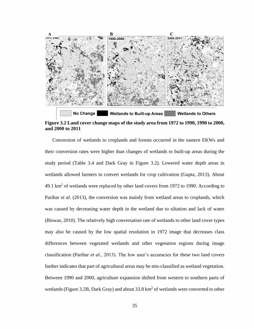
Figure 3.2 Land cover change maps of the study area from 1972 to 1990, 1990 to 2000,

and 2000 to 2011

Conversion of wetlands to croplands and forests occurred in the eastern EKWs and

their conversion rates were higher than changes of wetlands to built-up areas during the

study period (Table 3.4 and Dark Gray in Figure 3.2). Lowered water depth areas in

wetlands allowed farmers to convert wetlands for crop cultivation (Gupta, 2013). About

49.1 km2 of wetlands were replaced by other land covers from 1972 to 1990. According to

Parihar et al. (2013), the conversion was mainly from wetland areas to croplands, which

was caused by decreasing water depth in the wetland due to siltation and lack of water

(Biswas, 2010). The relatively high conversation rate of wetlands to other land cover types

may also be caused by the low spatial resolution in 1972 image that decreases class

differences between vegetated wetlands and other vegetation regions during image

classification (Parihar et al., 2013). The low user’s accuracies for these two land covers

further indicates that part of agricultural areas may be mis-classified as wetland vegetation.

Between 1990 and 2000, agriculture expansion shifted from western to southern parts of

wetlands (Figure 3.2B, Dark Gray) and about 33.8 km2 of wetlands were converted to other

36

land cover types. The conversion rate decreased slightly in the period from 2000 to 2011

when about 25.7 km2 other land types increased at the expense of wetlands.

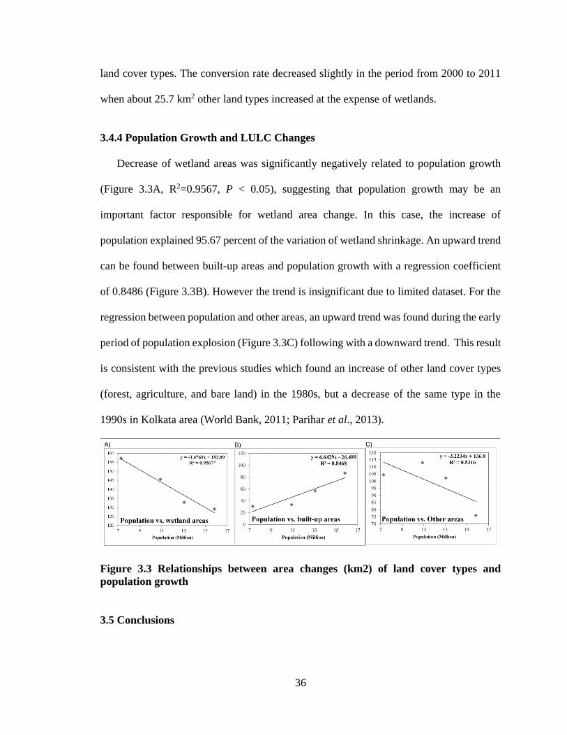
3.4.4 Population Growth and LULC Changes

Decrease of wetland areas was significantly negatively related to population growth

(Figure 3.3A, R2=0.9567, P < 0.05), suggesting that population growth may be an

important factor responsible for wetland area change. In this case, the increase of

population explained 95.67 percent of the variation of wetland shrinkage. An upward trend

can be found between built-up areas and population growth with a regression coefficient

of 0.8486 (Figure 3.3B). However the trend is insignificant due to limited dataset. For the

regression between population and other areas, an upward trend was found during the early

period of population explosion (Figure 3.3C) following with a downward trend. This result

is consistent with the previous studies which found an increase of other land cover types

(forest, agriculture, and bare land) in the 1980s, but a decrease of the same type in the

1990s in Kolkata area (World Bank, 2011; Parihar et al., 2013).

Figure 3.3 Relationships between area changes (km2) of land cover types and

population growth

3.5 Conclusions

37

Kolkata city in eastern India has seen unprecedented growth in recent years and in the

process a lot of the wetlands bordering the city have been transformed into built-up and

other land cover types. In this study four remotely sensed images (1972 – 2011) were used

to delineate the temporal and spatial patterns of wetland conversion to built-up areas or to

other types of land cover. The satellite data were processed using GeOBIA method and

post-classification comparison. GeOBIA as a classification technique using shape,

adjacency, and topological entities is increasingly becoming a better method than the

traditional pixel based classification. Accuracy assessment of classification indicated that

GeOBIA can provide accurate land cover conversion information with overall accuracies

ranging from 81.3 percent to 89.9 percent for the four classified images. The study suggests

a rapid decrease of wetland areas in EKWs due to an expansion of urban areas and other

land cover types (i.e. croplands, forests, and bare land). According to post-classification,

about 24.5 percent of wetlands have been converted to built-up areas over the past 39 years

change and the conversion rates increased with each time period analyzed. Western EKWs

showed a higher rate of area change than other parts of the study area. Conversion of

wetlands to other land cover types is also a reason for wetland shrinkage in EKWs, which

occurred mainly in eastern and southern parts of EKWs. The categorical estimation of

EKWs LULC conversion is a much needed assessment aligned with rapidly growing urban

development in the global south. It will help in understanding the land-atmospheric

dynamics, social and economic transitions in vulnerable areas like EKWs. To further utilize

this study EKWs LULC classification will be fed into the Weather Research and

Forecasting (WRF) model (Skamarock et al., 2008) to investigate the role of wetland

conversion in influencing the microclimatic variability in and around Kolkata City. Studies

38

like the above are a step further into quantifying the impacts of population pressure on

resources and land cover types which will help plan better for a sustainable future in fast

growing developing world urban areas.

39

3.6 Reference

Baker, B. A., Warner, T. A., Conley, J. F., & McNeil, B. E. (2013). Does spatial resolution

matter? A multi-scale comparison of object-based and pixel-based methods for

detecting change associated with gas well drilling operations. International Journal


Balçik, F. B. (2014). Determining the impact of urban components on land surface

temperature of Istanbul by using remote sensing indices. Environmental Monitoring

and Assessment, 186(2), 859–872. doi:10.1007/s10661-013-3427-5

Bartzen, B. A., Dufour, K. W., Clark, R. G., & Caswell, F. D. (2010). Trends in agricultural

impact and recovery of wetlands in prairie Canada. Ecological Application, 20(2),

525–538.

Bhatta, B. (2009). Analysis of urban growth pattern using remote sensing and GIS: a case

study of Kolkata, India. International Journal of Remote Sensing, 30(18), 4733–4746.

doi:10.1080/01431160802651967

Biswas, A. (2010). The spatial evaluation of sustainability in urban growth : measurement,

analysis and approach for south – east region of Kolkata, India, 1–8. Retrieved from

http://rdarc.itakura.toyo.ac.jp/webdav/ask/public/ACP2010/2.pdf

Bolca, M., Turkyilmaz, B., Kurucu, Y., Altinbas, U., Esetlili, M. T., & Gulgun, B. (2007).

Determination of impact of urbanization on agricultural land and wetland land use in

Balçovas’ delta by remote sensing and GIS technique. Environmental Monitoring and

Assessment, 131(1-3), 409–19. doi:10.1007/s10661-006-9486-0

Campbell, J. B., & Wynne, R. H. (2011). Introduction to remote sensing. New York: The

Guilford Press.

Carlson, T. N., & Arthur, S. T. (2000). The impact of land use - land cover changes due to


and Planetary Change, 25(1-2), 49–65. doi:10.1016/S0921-8181(00)00021-7

Chen, X.-L., Zhao, H.-M., Li, P.-X., & Yin, Z.-Y. (2006). Remote sensing image – based

analysis of the relationship between urban heat island and land use/cover changes.

Remote Sensing of Environment, 104(2), 133–146. doi:10.1016/j.rse.2005.11.016

Cui, B., Li, X., & Zhang, K. (2010). Classification of hydrological conditions to assess

water allocation schemes for Lake Baiyangdian in North China. Journal of Hydrology,

385(1-4), 247–256. doi:10.1016/j.jhydrol.2010.02.026

Cui, B., Yang, Q., Yang, Z., & Zhang, K. (2009). Evaluating the ecological performance

of wetland restoration in the Yellow River Delta, China. Ecological Engineering,

35(7), 1090–1103. doi:10.1016/j.ecoleng.2009.03.022

40

Dingle Robertson, L., & King, D. J. (2011). Comparison of pixel- and object-based

classification in land cover change mapping. International Journal of Remote Sensing,

32(6), 1505–1529. doi:10.1080/01431160903571791

Dronova, I., Gong, P., & Wang, L. (2011). Object-based analysis and change detection of

major wetland cover types and their classification uncertainty during the low water

period at Poyang Lake, China. Remote Sensing of Environment, 115(12), 3220–3236.

doi:10.1016/j.rse.2011.07.006

Gao, B. (1996). NDWI – a normalized difference water index for remote sensing of

vegetation liquid water from space. Remote Sensing of Environment, 58, 257–266.

Gupta, S. (2013). Changing land-use of East Kolkata Wetland, India. International Journal

of Applied Research and Studies, II(3), 1–8.


wetlands in Eastern Europe: vulnerability, adaptation and policy. Climate Change, 36,

107–121.

Howat, I. M., & Eddy, A. (2011). Multi-decadal retreat of Greenland’s marine-terminating

glaciers. Journal of Glaciology, 57, 389–396.

Jensen, J. R. (2006). Remote sensing of the environment: an earth resource perspective.

New Jersey: Prentice Hall, Upper Saddle River.

Li, X., Cui, B., Yang, Q., Tian, H., Lan, Y., Wang, T., & Han, Z. (2012). Detritus quality

controls macrophyte decomposition under different nutrient concentrations in a

eutrophic shallow lake, North China. PloS One, 7(7), e42042.

doi:10.1371/journal.pone.0042042

Mitra, C., Shepherd, J. M., & Jordan, T. (2012). On the relationship between the


India. International Journal of Climatology, 32(9), 1443–1454. doi:10.1002/joc.2366

Mitsch, W. J., & Gosselink, J. G. (2007). Wetlands. Program. John Wiley & Sons, Inc.

Moffett, K. B., & Gorelick, S. M. (2013). Distinguishing wetland vegetation and channel

features with object-based image segmentation. International Journal of Remote

Sensing, 34(4), 1332–1354. doi:10.1080/01431161.2012.718463

Munyati, C. (2000). Wetland change detection on the Kafue Flats, Zambia, by

classification of a multitemporal remote sensing image dataset. International Journal


41


wetland dynamics a post-classification change detection analysis of the East Kolkata

Wetlands using open source satellite data. Geocarto International, 28(3), 273–287.

Rijsberman, F., & De Silva, S. (2003). Sustainable agriculture and wetlands. In J.

Verhoeven, B. Beltman, R. Bobbink, & D. Whigham (Eds.), Wetlands and natural

resource management (pp. 33–52). Heidelberg: Springer.

Skamarock, W. C., Klemp, J. B., Dudhia, J., Gill, D. O., Barker, D. M., Duda, M. G.,

Huang, X. Y., Wang, W., Powers, J. G. (2008). A description of the advanced research

WRF version 3 NCAR/TN-475+STR.

UN Habitat. (2013). State of the world’s cities 2012/2013: Prosperity of cities (p. 135).

Washington, DC.

United Nations. (2005). World urbanization prospects, the 2005 revision. New York.

Retrived from

http://www.un.org/esa/population/publications/WUP2005/2005WUPHighlights_Fin

al_Report.pdf

World Bank. (2011). India – Vulnerability of Kolkata metropolitan area to increased

precipitation in a changing climate. Washington, DC: World Bank. Retrieved from

http://documents.worldbank.org/curated/en/2011/06/15781516/india-vulnerability-

kolkata-metropolitan-area-increased-precipitation-changing-climate

Wright, C., & Gallant, A. (2007). Improved wetland remote sensing in Yellowstone

National Park using classification trees to combine TM imagery and ancillary

environmental data. Remote Sensing of Environment, 107(4), 582–605.

doi:10.1016/j.rse.2006.10.019

Yuan, F., Sawaya, K. E., Loeffelholz, B. C., & Bauer, M. E. (2005). Land cover

classification and change analysis of the Twin Cities (Minnesota) Metropolitan Area

by multitemporal Landsat remote sensing. Remote Sensing of Environment, 98(2-3),

317–328. doi:10.1016/j.rse.2005.08.006

42

4. Impact of wetland area decrease on microclimate as detected by

Weather Research and Forecasting (WRF) Model

4.1 Introduction

Microclimate is the climatic conditions on a specific local scale. It synthesizes “the

ambient physical conditions due to either atmospheric variables or exchanges with other

bodies over a period of time representative of all the conditions determined by the natural

and manmade forcing factors” (Camuffo 1998, p8). The atmospheric variables including

temperature, humidity, and precipitation are important for human existence and can be

influenced by human activities (Hartig et al. 1997; McMichael et al. 2006). Meanwhile,

microclimate also affects the ecological processes of ecosystems. Elevated temperature

tends to increase crop yields (Stone et al. 1999; van Ittersum et al. 2003) and to precede

phenological events of plants such as leafing, flowering, and shooting (Estrella et al. 2007).

Precipitation and soil moisture play important roles in controlling the plant productivity

and regional nutrient cycling (Schuur 2003; Heisler-White et al. 2008).

Land use/land cover (LULC) dynamics is one of the main factors causing changes

in microclimate in recent decades (Rahman, 2014). Wetlands are essential components of

microclimate because they have their own characteristic moisture cycles due to the specific

aquatic plants present (Carrington et al. 2001). Conversion of wetland areas to agricultural

lands was a main reason for wetland loss in the world due to the increased population

43

pressures, and the conversion rate has been further accelerated dramatically in the 20th

century due to reductions in runoff and increase in evapotranspiration under climate change

(Hartig et al. 1997; Rijsberman and De Silva, 2006). The drainage ditches built for

agriculture have significantly lowered the water table of wetlands and reduced water-

storage capacity, changing local hydrological cycling such as evapotranspiration and

runoff (Bartzen et al. 2010). Moreover, Marshall et al. (2004) suggested that shifts of

wetlands to croplands have resulted in or increased the severity of freezes in South Florida

because decreases in water depth influenced the effective heat capacity and lowered the

minimum temperature. Besides water storage, changes in vegetation types can also

influence precipitation and local water cycling due to differences in evapotranspiration

(Kutzbach et al. 1996; Carrington et al. 2001).

Decreases in wetland regions not only alter compositions of plants but also

influence the permeability of surface land. Conversion of wetland to built-up areas

increases the impervious surfaces that increase surface runoff, and therefore impacting the

water cycle of the region. Along with increased built-up areas elevated temperature can

also be observed due to urban heat island effect, which is mainly caused by elevated heat

emissions from human-related sources and reduced vegetation covers (Weng et al. 2004;

Chen et al. 2006; Tan et al. 2009). Carlson and Arthur (2000) investigated the effects of

LULC dynamics on microclimate at three different locations by satellite imagery in

Philadelphia, PA, U.S. Experimental results suggested that areas with large water bodies

were sensitive to built-up area expansion. The temperature increased 38% while the

moisture decreased 14% when a region changed from an open water body to 30%

urbanized area (Carlson and Arthur 2000).

44

Influences on microclimate due to LULC change can be explored by the Weather

Research and Forecasting (WRF) model (Hong et al. 2009; Mahmood et al. 2011). The

WRF model is a fully compressible, non-hydrostatic numerical weather prediction system

used for weather forecasting and atmospheric research (Skamarock et al., 2008). It has been

developed by a community of government agencies and researchers. The model is able to

conduct both real data simulations (observations, analyses) and idealized atmospheric

condition predictions and to serve a wide range of application areas from meters to

thousands of kilometers (http://www.wrf-model.org/). The efficiency of the model has

been proved in several research fields including air quality prediction (Misenis and Zhang

2010; Zhang et al. 2010a), fire-weather simulation (Mölders 2008), extreme weather

simulation (Wang et al. 2006; Evans and McCabe 2010), as well as climate change issues

(Jiménez et al. 2011; Zaitchik et al. 2013).

Various studies have used the WRF model to successfully assess the impact of

LULC dynamics on microclimate. As discussed above, changes in land cover can

significantly alter the microclimate of a region. The WRF model is highly sensitive to

vegetation fluctuations and land use changes (Hong et al. 2009; Mahmood et al. 2011).

Zhang et al. (2010b) utilized WRF model to investigate the microclimate change in China.

They found that conversion of cropland to urban space increased both temperature and

precipitation but decreased surface humidity with a stronger influence in summer than in

winter. Mahmood et al. (2011) used the WRF model by combining it with the National

Center for Atmospheric Research's (NCAR) fifth generation mesoscale model (MM5)

model to investigate the responses of climatic indices on LULC dynamics in Western

Kentucky, USA. Results suggested that changes in land use influence latent heat flux,

http://www.wrf-model.org/

45

temperature, relative humidity, as well as wind. However, the impacts were diminished

during nighttime. More specifically, by incorporating Noah Urban Canopy together with

WRF model, Grossman-Clarke et al. (2010) explored how much urban expansion

contributes to an increase in near-surface air temperature and they observed the maximum

temperature increase when irrigated agricultural lands were replaced by suburban areas.

Under the pressure of rapid population growth, it is easy to expand agricultural

and built-up areas at the expense of wetlands because drained wetlands provide perfect

sources for arable lands in dry season (Scoones 1991). It is necessary to evaluate how

greatly the microclimate can be altered due to wetland shrinkage as that could influence

economic growth and have impacts on human health. In this chapter, WRF model was

applied to investigate influences of LULC change and wetland conversion on temperature,

precipitation, latent heat flux, sensible heat flux, and albedo at Kolkata city. The study

will be of first order significance in assessing the role of urban area increase on Kolkata’s

local hydrology and climate.

4.2 Material and Methodology

4.2.1 Methods

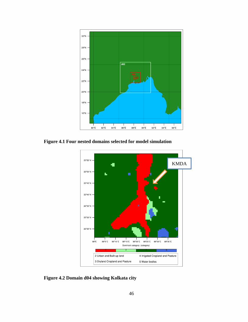
46

Figure 4.1 Four nested domains selected for model simulation

Figure 4.2 Domain d04 showing Kolkata city

KMDA

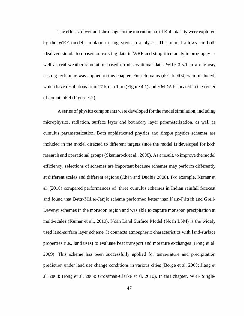
47

The effects of wetland shrinkage on the microclimate of Kolkata city were explored

by the WRF model simulation using scenario analyses. This model allows for both

idealized simulation based on existing data in WRF and simplified analytic orography as

well as real weather simulation based on observational data. WRF 3.5.1 in a one-way

nesting technique was applied in this chapter. Four domains (d01 to d04) were included,

which have resolutions from 27 km to 1km (Figure 4.1) and KMDA is located in the center

of domain d04 (Figure 4.2).

A series of physics components were developed for the model simulation, including

microphysics, radiation, surface layer and boundary layer parameterization, as well as

cumulus parameterization. Both sophisticated physics and simple physics schemes are

included in the model directed to different targets since the model is developed for both

research and operational groups (Skamarock et al., 2008). As a result, to improve the model

efficiency, selections of schemes are important because schemes may perform differently

at different scales and different regions (Chen and Dudhia 2000). For example, Kumar et

al. (2010) compared performances of three cumulus schemes in Indian rainfall forecast

and found that Betts-Miller-Janjic scheme performed better than Kain-Fritsch and Grell-

Devenyi schemes in the monsoon region and was able to capture monsoon precipitation at

multi-scales (Kumar et al., 2010). Noah Land Surface Model (Noah LSM) is the widely

used land-surface layer scheme. It connects atmospheric characteristics with land-surface

properties (i.e., land uses) to evaluate heat transport and moisture exchanges (Hong et al.

2009). This scheme has been successfully applied for temperature and precipitation

prediction under land use change conditions in various cities (Borge et al. 2008; Jiang et

al. 2008; Hong et al. 2009; Grossman-Clarke et al. 2010). In this chapter, WRF Single-

48

Moment 5-class microphysical scheme was applied to predict water vapor and condensate

as cloud, rain, cloud ice and precipitation ice (Skamarock et al. 2008). The Noah LSM

scheme was selected as land-surface layer scheme. The rapid radiative transfer model for

GCM (RRTMG) was used to determine transfer processes of longwave radiation (Iacono

et al. 2008) and Dudhia scheme was chosen for shortwave radiation. Yonsei University

scheme was applied to solve turbulent vertical fluxes throughout the planetary boundary

layer (PBL) (Hu et al. 2010). For the cumulus scheme, Betts-Miller-Janjic scheme was

used in this chapter. Some details of the model configuration were listed in Table 4.1.

Table 4.1 Model configuration and physics schemes during simulation

Number of domains 4

Resolution 27 km (domain d01), 9 km (domain d02),

3 km (domain d03), 1 km (domain d04)

Number of grid points 70 × 70 (all domains)

Map projection Mercator

Central point of the domain Central latitude: 22.66° N

Central longitude: 88.33° E

Microphysics scheme Single-Moment 5-class microphysical

scheme

Land-surface layer scheme Noah land surface model

Radiation scheme (long wave) Rapid radiative transfer model for GCM

(RRTMG)

Radiation scheme (short wave) Dudhia scheme

Boundary layer physics Yonsei University scheme

49

Cumulus convection scheme Betts-Miller-Janjic scheme

4.2.1.1 Scenario Analyses

Scenario analyses were conducted to quantify contributions of wetland conversion

to microclimate changes. This study used three scenarios running from November 2011 to

January 2012. The reason for choosing this period is because this period is the dry season

in Kolkata city, which can reduce anomalous precipitation due to the influence of monsoon

rainfall.

Scenario 1: Real weather simulation

A real weather running was first applied to simulate microclimate in KMDA during

the chosen period. This process used the 33-category U.S. Geological Survey (USGS) Land

Use/Land Cover system as LULC data for Kolkata city.

Scenario 2: wetland and cropland to built-up conversion

The assumption in this scenario was that conversions of wetlands and croplands to

built-up areas are the assumed LULC change during study period. Other LULC patterns

are kept unchanged similar to LULC patterns in 2011. To achieve this object, parameters

of “dryland cropland and pasture”, “irrigated cropland and pasture”, “herbaceous wetland”,

and “wooded wetland” were changed to parameters of “urban and build-up land” in

LANDUSE.TBL and VEGPARM.TBL and re-run the weather simulation.

Scenario 3: wetland and dryland cropland to irrigate cropland conversion

The assumption in this scenario was that conversions of wetlands and dryland

cropland to irrigate cropland are the assumed LULC change during study period. Other

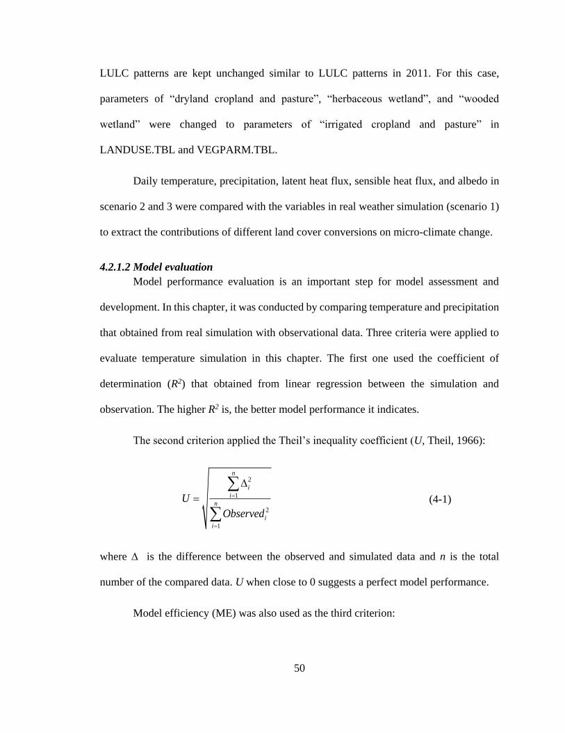
50

LULC patterns are kept unchanged similar to LULC patterns in 2011. For this case,

parameters of “dryland cropland and pasture”, “herbaceous wetland”, and “wooded

wetland” were changed to parameters of “irrigated cropland and pasture” in

LANDUSE.TBL and VEGPARM.TBL.

Daily temperature, precipitation, latent heat flux, sensible heat flux, and albedo in

scenario 2 and 3 were compared with the variables in real weather simulation (scenario 1)

to extract the contributions of different land cover conversions on micro-climate change.

4.2.1.2 Model evaluation

Model performance evaluation is an important step for model assessment and

development. In this chapter, it was conducted by comparing temperature and precipitation

that obtained from real simulation with observational data. Three criteria were applied to

evaluate temperature simulation in this chapter. The first one used the coefficient of

determination (R2) that obtained from linear regression between the simulation and

observation. The higher R2 is, the better model performance it indicates.

The second criterion applied the Theil’s inequality coefficient (U, Theil, 1966):

2

1

2

1

n

i

i

n

i

i

U

Observed

(4-1)

where ∆ is the difference between the observed and simulated data and n is the total

number of the compared data. U when close to 0 suggests a perfect model performance.

Model efficiency (ME) was also used as the third criterion:

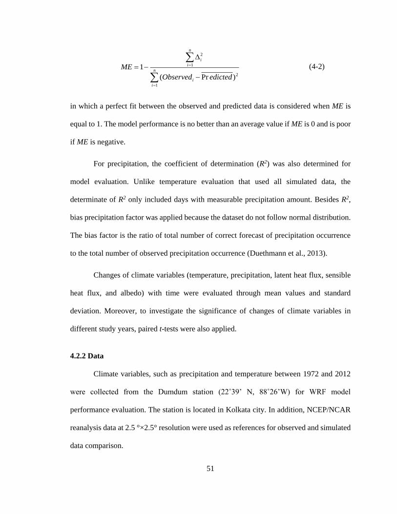
51

2

1

2

1

1

( Pr )

n

i

i

n

i

i

ME

Observed edicted

(4-2)

in which a perfect fit between the observed and predicted data is considered when ME is

equal to 1. The model performance is no better than an average value if ME is 0 and is poor

if ME is negative.

For precipitation, the coefficient of determination (R2) was also determined for

model evaluation. Unlike temperature evaluation that used all simulated data, the

determinate of R2 only included days with measurable precipitation amount. Besides R2,

bias precipitation factor was applied because the dataset do not follow normal distribution.

The bias factor is the ratio of total number of correct forecast of precipitation occurrence

to the total number of observed precipitation occurrence (Duethmann et al., 2013).

Changes of climate variables (temperature, precipitation, latent heat flux, sensible

heat flux, and albedo) with time were evaluated through mean values and standard

deviation. Moreover, to investigate the significance of changes of climate variables in

different study years, paired t-tests were also applied.

4.2.2 Data

Climate variables, such as precipitation and temperature between 1972 and 2012

were collected from the Dumdum station (22˚39’ N, 88˚26’W) for WRF model

performance evaluation. The station is located in Kolkata city. In addition, NCEP/NCAR

reanalysis data at 2.5 °×2.5° resolution were used as references for observed and simulated

data comparison.

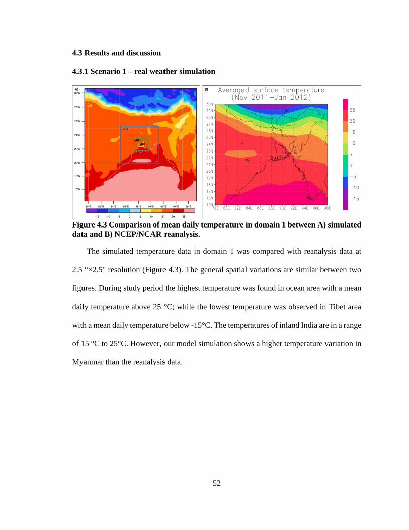
52

4.3 Results and discussion

4.3.1 Scenario 1 – real weather simulation

Figure 4.3 Comparison of mean daily temperature in domain 1 between A) simulated

data and B) NCEP/NCAR reanalysis.

The simulated temperature data in domain 1 was compared with reanalysis data at

2.5 °×2.5° resolution (Figure 4.3). The general spatial variations are similar between two

figures. During study period the highest temperature was found in ocean area with a mean

daily temperature above 25 °C; while the lowest temperature was observed in Tibet area

with a mean daily temperature below -15°C. The temperatures of inland India are in a range

of 15 °C to 25°C. However, our model simulation shows a higher temperature variation in

Myanmar than the reanalysis data.

53

Figure 4.4 Comparison of mean daily latent heat flux in domain 1 between A)

simulated data and B) NCEP/NCAR reanalysis.

Figure 4.5 Comparison of mean daily sensible heat flux in domain 01 between A)

simulated data and B) NCEP/NCAR reanalysis.

Simulated heat fluxes by WRF were also evaluated against the reanalysis data. In this

study, latent heat flux refers to the energy flux exchange between land surface and the

atmosphere that is used for phase changes of water through evapotranspiration and

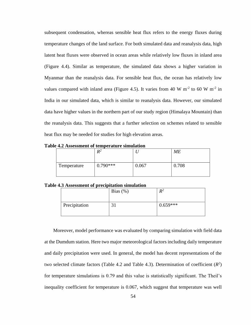
54

subsequent condensation, whereas sensible heat flux refers to the energy fluxes during

temperature changes of the land surface. For both simulated data and reanalysis data, high

latent heat fluxes were observed in ocean areas while relatively low fluxes in inland area

(Figure 4.4). Similar as temperature, the simulated data shows a higher variation in

Myanmar than the reanalysis data. For sensible heat flux, the ocean has relatively low

values compared with inland area (Figure 4.5). It varies from 40 W m-2 to 60 W m-2 in

India in our simulated data, which is similar to reanalysis data. However, our simulated

data have higher values in the northern part of our study region (Himalaya Mountain) than

the reanalysis data. This suggests that a further selection on schemes related to sensible

heat flux may be needed for studies for high elevation areas.

Table 4.2 Assessment of temperature simulation

R2 U ME

Temperature 0.790*** 0.067 0.708

Table 4.3 Assessment of precipitation simulation

Bias (%) R2

Precipitation 31 0.659***

Moreover, model performance was evaluated by comparing simulation with field data

at the Dumdum station. Here two major meteorological factors including daily temperature

and daily precipitation were used. In general, the model has decent representations of the

two selected climate factors (Table 4.2 and Table 4.3). Determination of coefficient (R2)

for temperature simulations is 0.79 and this value is statistically significant. The Theil’s

inequality coefficient for temperature is 0.067, which suggest that temperature was well

55

simulated by the model. In addition, ME value (0.708) is close to 1 and further indicates

that the real-simulation reasonable matched observed data. Determination of coefficient

for precipitation simulation is 0.659 and also suggested that the modeled precipitation

events matched observation well. Bias between model simulation and field data indicate

that there are some discrepancies between modeled and simulated precipitation.

The WRF model has been widely used in simulating regional meteorological

conditions (Evans et al., 2012; Shrivastava et al., 2015; Yang et al., 2015). A variety of

evaluation methodologies have been developed to evaluate the performance of the model

(Jankov et al., 2005). Results of the evolution in this study is consistent with previous

studies that shows less bias in temperature simulation than that in precipitation (Evans et

al., 2012). In addition to the uncertainties in input land cover data and temporal/spatial

resolution multiple driving forces, physical options in model parameterization could be an

important cause for the discrepancies between model simulation and observation

(Shrivastava et al., 2015). In the future, model performance could be potentially improved

by optimizing multiple parameterization schemes (Lee et al., 2011).

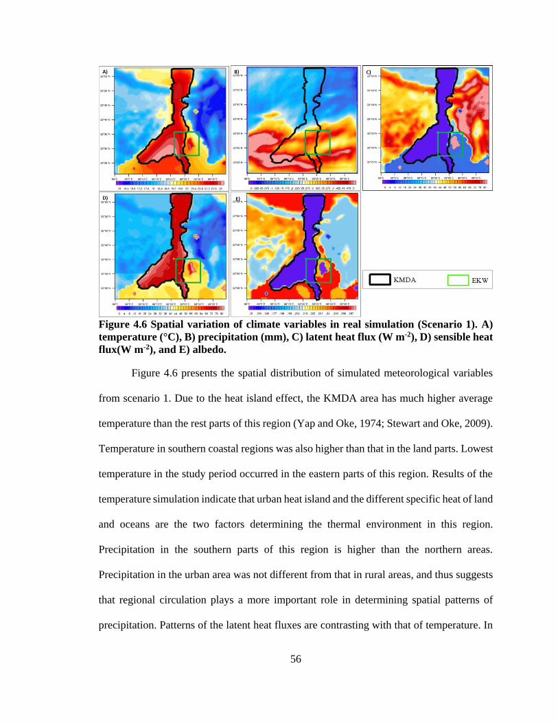
56

Figure 4.6 Spatial variation of climate variables in real simulation (Scenario 1). A)


flux(W m-2), and E) albedo.

Figure 4.6 presents the spatial distribution of simulated meteorological variables

from scenario 1. Due to the heat island effect, the KMDA area has much higher average

temperature than the rest parts of this region (Yap and Oke, 1974; Stewart and Oke, 2009).

Temperature in southern coastal regions was also higher than that in the land parts. Lowest

temperature in the study period occurred in the eastern parts of this region. Results of the

temperature simulation indicate that urban heat island and the different specific heat of land

and oceans are the two factors determining the thermal environment in this region.

Precipitation in the southern parts of this region is higher than the northern areas.

Precipitation in the urban area was not different from that in rural areas, and thus suggests

that regional circulation plays a more important role in determining spatial patterns of

precipitation. Patterns of the latent heat fluxes are contrasting with that of temperature. In

57

the KMDA region and the southern parts of the study area where heat fluxes from land to

the atmosphere are low, average temperatures are mainly over 19ºC. Conversely, in the rest

cropland regions which show much higher latent heat flux (generally over 40 W m-2),

temperatures were generally below 19ºC. Low water contents in soils of built-up regions

were mainly responsible for the low latent heat fluxes in urban regions. Contrasting

patterns between latent heat flux and temperature is in line with the previous investigations

that reported the cooling effects of plantation relative to built-up regions. However, it

should be noted that even latent heat flux at the EKW region was high, it did not result in

low temperature in this region. Instead, temperatures in this area are comparable with that

in the urban regions. Possible explanation can be derived from the EKW distribution of the

sensible latent flux figure. As depicted in figure 4.6D, water body of EKW region had high

sensible heat fluxes during winter time, and thus resulted in the relatively higher

temperature (Sánchez-Carrillo et al., 2004). Due to the low specific heat in urban area,

urban areas tend to be net source of sensible heat, whereas the rest parts of the study area

tended to obtain energy from the atmosphere to support evapotranspiration.

4.3.2 Scenario comparison

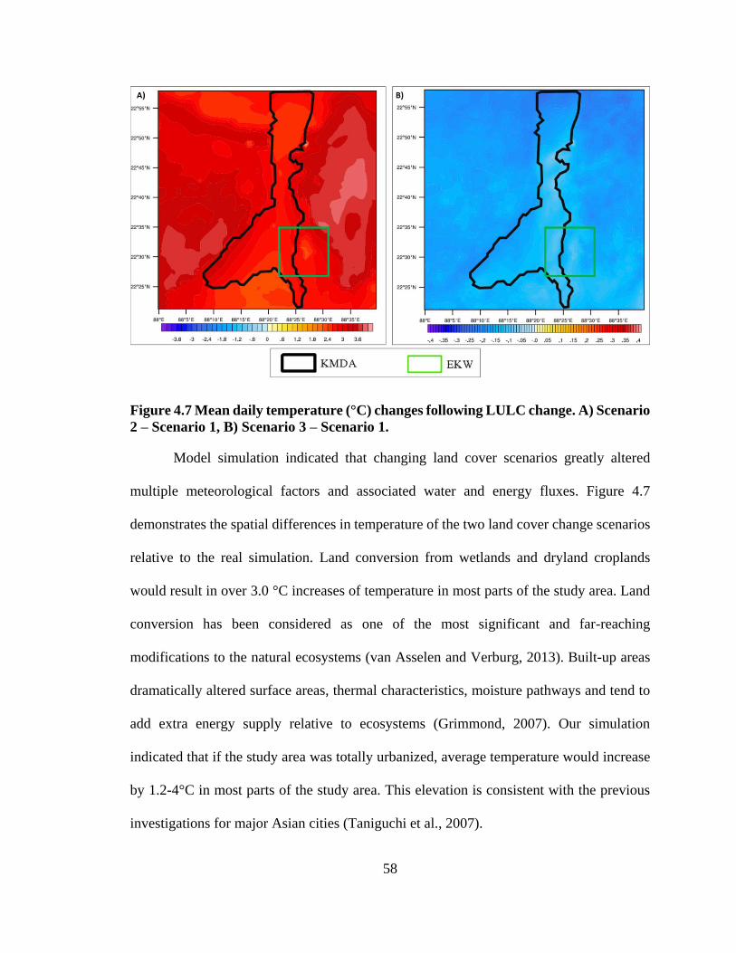
58

Figure 4.7 Mean daily temperature (°C) changes following LULC change. A) Scenario

2 – Scenario 1, B) Scenario 3 – Scenario 1.

Model simulation indicated that changing land cover scenarios greatly altered

multiple meteorological factors and associated water and energy fluxes. Figure 4.7

demonstrates the spatial differences in temperature of the two land cover change scenarios

relative to the real simulation. Land conversion from wetlands and dryland croplands

would result in over 3.0 °C increases of temperature in most parts of the study area. Land

conversion has been considered as one of the most significant and far-reaching

modifications to the natural ecosystems (van Asselen and Verburg, 2013). Built-up areas

dramatically altered surface areas, thermal characteristics, moisture pathways and tend to

add extra energy supply relative to ecosystems (Grimmond, 2007). Our simulation

indicated that if the study area was totally urbanized, average temperature would increase

by 1.2-4°C in most parts of the study area. This elevation is consistent with the previous

investigations for major Asian cities (Taniguchi et al., 2007).

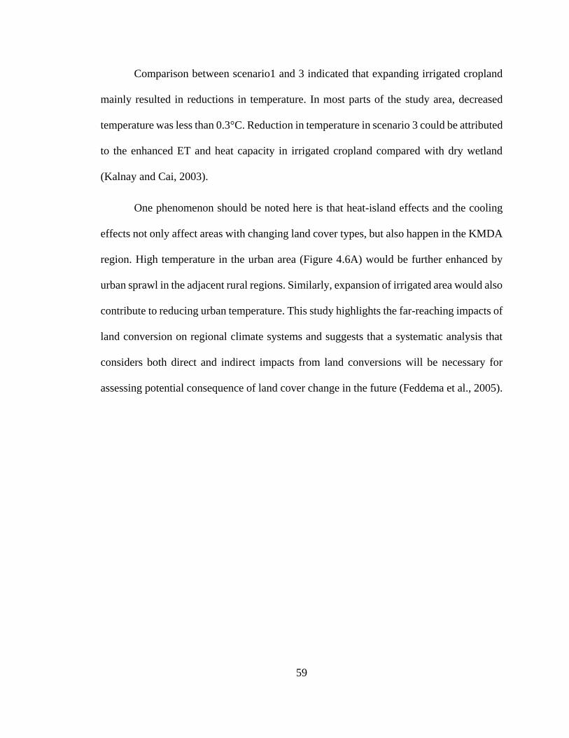
59

Comparison between scenario1 and 3 indicated that expanding irrigated cropland

mainly resulted in reductions in temperature. In most parts of the study area, decreased

temperature was less than 0.3°C. Reduction in temperature in scenario 3 could be attributed

to the enhanced ET and heat capacity in irrigated cropland compared with dry wetland

(Kalnay and Cai, 2003).

One phenomenon should be noted here is that heat-island effects and the cooling

effects not only affect areas with changing land cover types, but also happen in the KMDA

region. High temperature in the urban area (Figure 4.6A) would be further enhanced by

urban sprawl in the adjacent rural regions. Similarly, expansion of irrigated area would also

contribute to reducing urban temperature. This study highlights the far-reaching impacts of

land conversion on regional climate systems and suggests that a systematic analysis that

considers both direct and indirect impacts from land conversions will be necessary for

assessing potential consequence of land cover change in the future (Feddema et al., 2005).

60

Figure 4.8 Mean daily precipitation changes (mm) following LULC change. A)

Scenario 2 – Scenario 1, B) Scenario 3 – Scenario 1.

Impacts of land cover changes on precipitation are complicated (Mahmood et al.,

2010). Figure 4.8 shows that land cover conversion induced both increased and decreased

precipitation in the study area. For urbanization scenario, precipitation center tends to move

northeastern ward and leads to increased rainfall in the northeastern parts of this region.

This may be caused by downwind effect. In real weather simulation, the precipitation is

extremely higher in Jan. 7th and Jan 8th than in other days with southwest winds. The low-

level prevailing wind tends to advect the moisture and low level convergence downstream

urbanized area and thus leads to enhanced precipitation some distance downwind of urban

areas (Shepherd et al., 2002). For the EKW domain, precipitation is mainly enhanced,

except for in the central areas where wetlands are located. For the KMDA domain, rainfall

was generally stimulated in the south, but reduced in the central-north areas. Northern

61

regions of the study area also received higher rainfall relative to the control simulation.

Decreased precipitation can be found in the southwestern parts of this region.

Impacts of urbanization on rainfall patterns have been widely documented,

especially for major metropolitan areas. In consistent with some of the previous

investigations, this study also shows that response of precipitation to urbanization is not as

evident as that of temperature (Tayanc and Toros, 1997). Underlying mechanisms

regulating rainfall response to urbanization have not been adequately explored yet.

Urbanization induces a series of complicated changes in land surface roughness, soil

moisture and the exchange of water and energy between land and the atmosphere (Lamptey

et al., 2005). These changes can either offset or enhance each other and thus further

complicate the spatial patterns of precipitation (Trusilova et al., 2008).

Expansion of irrigated cropland tends to move the precipitation center to the central

regions of the study area. Figure 4.8B suggests that most parts of the central and eastern

areas would experience enhanced rainfall. Reduced rainfall was mainly located in the

southwestern and northwestern parts of the study area. For the EKW domain, irrigated

cropland tends to enhance precipitation in most parts of this area. In the KMDA domain,

precipitation showed significant increases in the center of the city but decreases in northern

and southern parts of the city. In the southeast corner of the city, precipitation was

significantly reduced.

Previous studies have reported that expansion of irrigation has positive impacts on

precipitation (Wei et al., 2012). Increases in precipitation are possibly caused by enhanced

evapotranspiration following expanded irrigated land (Deangelis et al., 2010). Similar to

the impacts contributed by urbanization, precipitation changes in scenario 3 may also due

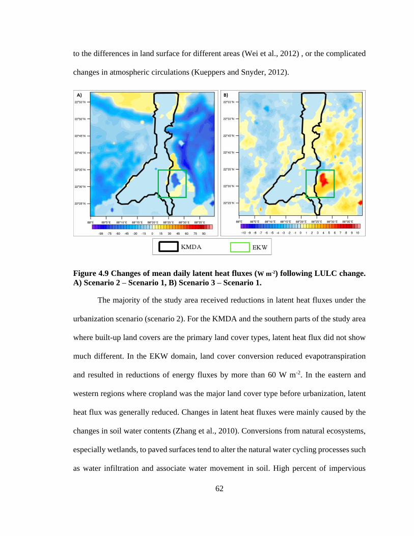
62

to the differences in land surface for different areas (Wei et al., 2012) , or the complicated

changes in atmospheric circulations (Kueppers and Snyder, 2012).

Figure 4.9 Changes of mean daily latent heat fluxes (W m-2) following LULC change.

A) Scenario 2 – Scenario 1, B) Scenario 3 – Scenario 1.

The majority of the study area received reductions in latent heat fluxes under the

urbanization scenario (scenario 2). For the KMDA and the southern parts of the study area

where built-up land covers are the primary land cover types, latent heat flux did not show

much different. In the EKW domain, land cover conversion reduced evapotranspiration

and resulted in reductions of energy fluxes by more than 60 W m-2. In the eastern and

western regions where cropland was the major land cover type before urbanization, latent

heat flux was generally reduced. Changes in latent heat fluxes were mainly caused by the

changes in soil water contents (Zhang et al., 2010). Conversions from natural ecosystems,

especially wetlands, to paved surfaces tend to alter the natural water cycling processes such

as water infiltration and associate water movement in soil. High percent of impervious

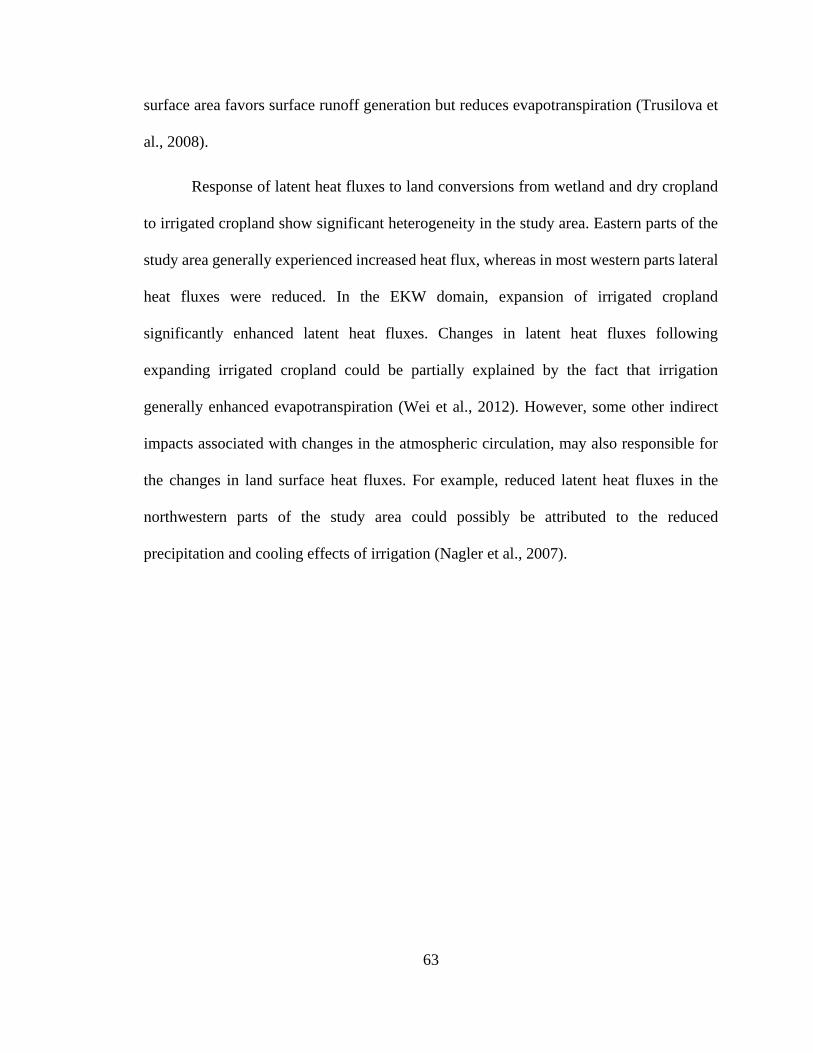
63

surface area favors surface runoff generation but reduces evapotranspiration (Trusilova et

al., 2008).

Response of latent heat fluxes to land conversions from wetland and dry cropland

to irrigated cropland show significant heterogeneity in the study area. Eastern parts of the

study area generally experienced increased heat flux, whereas in most western parts lateral

heat fluxes were reduced. In the EKW domain, expansion of irrigated cropland

significantly enhanced latent heat fluxes. Changes in latent heat fluxes following

expanding irrigated cropland could be partially explained by the fact that irrigation

generally enhanced evapotranspiration (Wei et al., 2012). However, some other indirect

impacts associated with changes in the atmospheric circulation, may also responsible for

the changes in land surface heat fluxes. For example, reduced latent heat fluxes in the

northwestern parts of the study area could possibly be attributed to the reduced

precipitation and cooling effects of irrigation (Nagler et al., 2007).

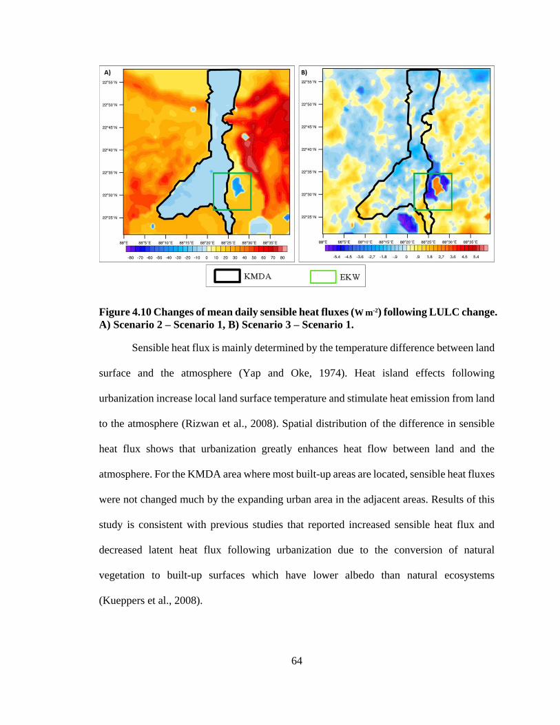
64

Figure 4.10 Changes of mean daily sensible heat fluxes (W m-2) following LULC change.

A) Scenario 2 – Scenario 1, B) Scenario 3 – Scenario 1.

Sensible heat flux is mainly determined by the temperature difference between land

surface and the atmosphere (Yap and Oke, 1974). Heat island effects following

urbanization increase local land surface temperature and stimulate heat emission from land

to the atmosphere (Rizwan et al., 2008). Spatial distribution of the difference in sensible

heat flux shows that urbanization greatly enhances heat flow between land and the

atmosphere. For the KMDA area where most built-up areas are located, sensible heat fluxes

were not changed much by the expanding urban area in the adjacent areas. Results of this

study is consistent with previous studies that reported increased sensible heat flux and

decreased latent heat flux following urbanization due to the conversion of natural

vegetation to built-up surfaces which have lower albedo than natural ecosystems

(Kueppers et al., 2008).

65

Although increasing irrigated croplands mainly reduced air temperature in this

region (Figure 4.7), changes in sensible heat fluxes are either positive or negative relative

to the unchanged land cover scenario. Figure 4.10 indicates that in the western and eastern

regions of this study area, sensible heat fluxes are mainly enhanced, whereas in the central

regions, the heat flux is mainly reduced. In the KMDA domain, where land cover is

consistent between the two simulations, sensible heat flux was also reduced and thus

suggested that irrigation activities in the local areas may affect energy fluxes in surrounding

areas (Stohlgren et al., 1998).

Figure 4.11 Changes of albedo following LULC change. A) Scenario 2 – Scenario 1,

B) Scenario 3 – Scenario 1

Albedo is the fraction of solar energy reflected from the Earth back to space. It can

be changed by land cover change. Royer et al. (1988) found a decrease in surface albedo

when vegetation converted to urban areas. The relatively low albedo in urban areas than

cropland may be caused by the multireflection effect between buildings (Wang et al., 2007).

Besides that, more aerosol emissions in urban area absorb solar shortwave radiation and

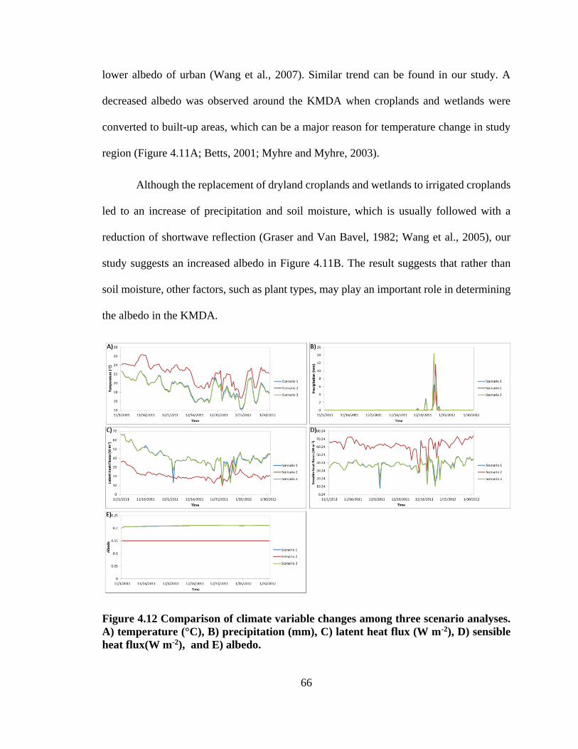
66

lower albedo of urban (Wang et al., 2007). Similar trend can be found in our study. A

decreased albedo was observed around the KMDA when croplands and wetlands were

converted to built-up areas, which can be a major reason for temperature change in study

region (Figure 4.11A; Betts, 2001; Myhre and Myhre, 2003).

Although the replacement of dryland croplands and wetlands to irrigated croplands

led to an increase of precipitation and soil moisture, which is usually followed with a

reduction of shortwave reflection (Graser and Van Bavel, 1982; Wang et al., 2005), our

study suggests an increased albedo in Figure 4.11B. The result suggests that rather than

soil moisture, other factors, such as plant types, may play an important role in determining

the albedo in the KMDA.

Figure 4.12 Comparison of climate variable changes among three scenario analyses.

A) temperature (°C), B) precipitation (mm), C) latent heat flux (W m-2), D) sensible

heat flux(W m-2), and E) albedo.

67

This study also checked the temporal patterns of major meteorological variables

from the three scenario simulations (Figure 4.12). Results indicated that scenario 1 and 3

generated similar temperature time series from the beginning of November, 2011 to the

end of January, 2012. In the two scenarios, temperatures generally had decreasing trends

with significant variability occurring in January of 2012. The study indicated that urban

sprawl could dramatically increase average temperature. Due to the changing albedo and

hydrological cycles, urban area tended to have higher temperature (Ren et al., 2008).

However, the temporal variation of temperature from scenario 2 is similar to that of the

other scenarios, and thus suggested that atmospheric circulation play the primary role in

determining temporal changes in temperature.

Winter is a dry season in India since most of the rainfall events occur in the

monsoon season (Krishnamurthy and Shukla, 2007). The three simulations agreed well in

that no precipitation occurs in November and December of 2011, which is similar to the

observational data. The simulations were also consistent in the occurrence of rainfall events

in January 2012. However, the magnitudes of rainfall were divergent from the three

simulations. For the two rainfall events occurred around December 20th and in the

beginning of January, scenario 1 and 3 had similar estimates. However, precipitations from

scenario 2 during these two events were significantly lower in the scenario 2 simulation.

Largest discrepancies among the three simulations occurred to the rainfall events occurs

around January 7th. For this event, scenarios (2 and 3) with changing land cover types

tended to induce heavy rainfalls compared with the real simulation.

Changing land covers could largely change the energy exchange between land and

the atmosphere (Douglas et al., 2006). For the latent heat flux, both scenario1 and 3 showed

68

similar temporal patterns which decreased with time during the study period. The temporal

trend was similar to that of temperature, and indicated that low temperature may reduce

evapotranspiration and associate energy fluxes in January of 2012 (Lamptey et al., 2005).

The two scenarios had very close estimates, especially in the last two months in 2011. In

January of 2012, latent energy flux was a bit higher than that of scenario 1, but their

temporal variability was almost identical. This study suggests that urbanization would

totally alter the exchange between land and the atmosphere (Kueppers and Snyder, 2012).

Increasing urban areas significantly reduced lateral heat fluxes relative to the other two

scenarios. In addition to the magnitude, temporal variability in scenario 2 was also much

lower than the other simulations.

In contrast to the patterns of latent heat flux, sensible heat fluxes demonstrated

increasing trends during the study period. Again, scenario 1 and 3 had similar temporal

patterns, but scenario 2 resulted in much higher sensible heat fluxes relative to the other

two simulations. Moreover, sensible heat fluxes following the urbanization scenario

increased greatly and suggested that urbanized land surfaces are important heat generating

source (Kitada et al., 1998).

Since albedo is determined by the land use covers, it only showed slightly

increasing trend temporal changes as land cover types were fixed for each simulation.

Albedo in scenario 1 and 3 were all around 0.21, and indicating that land conversion from

wetland and dry cropland to irrigated cropland did not significantly change the average

albedo of the entire region. However, urbanization at the expense of natural and agricultural

ecosystems tended to increase albedo.

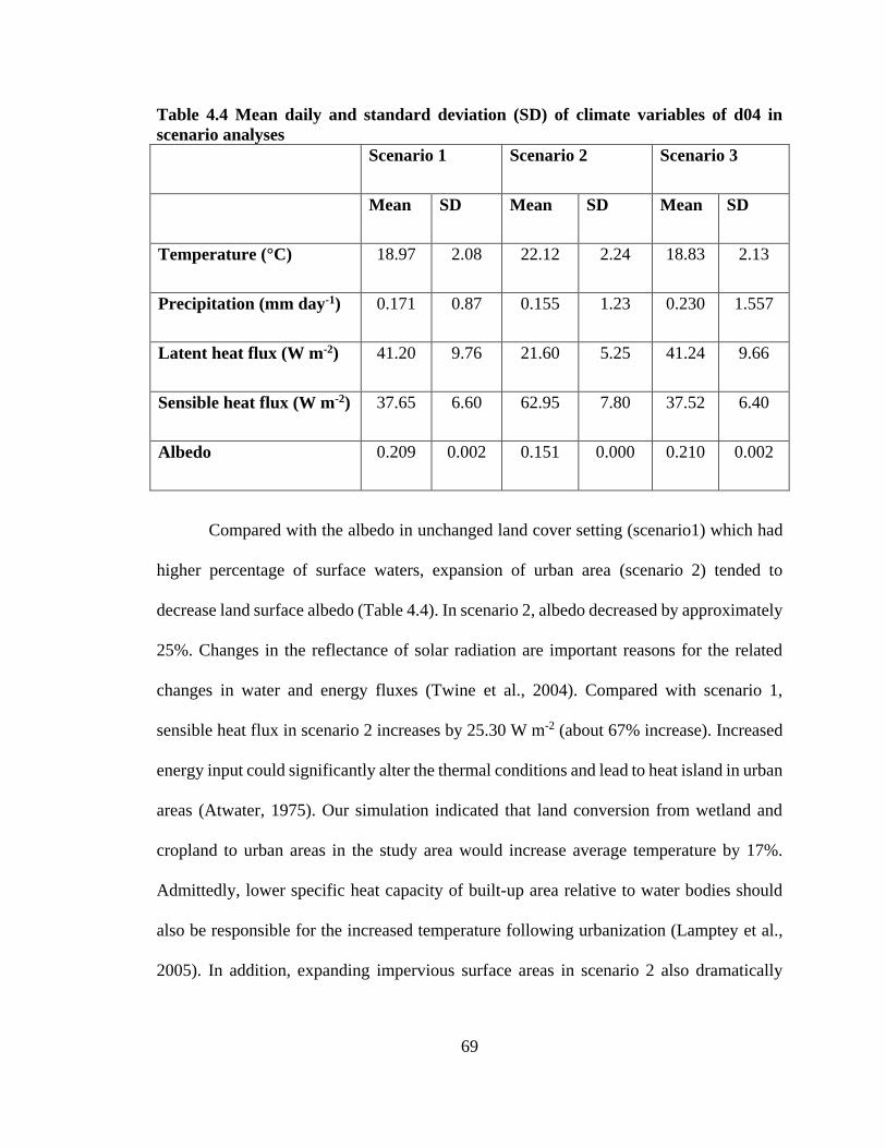
69

Table 4.4 Mean daily and standard deviation (SD) of climate variables of d04 in

scenario analyses

Scenario 1 Scenario 2 Scenario 3

Mean SD Mean SD Mean SD

Temperature (°C) 18.97 2.08 22.12 2.24 18.83 2.13

Precipitation (mm day-1) 0.171 0.87 0.155 1.23 0.230 1.557

Latent heat flux (W m-2) 41.20 9.76 21.60 5.25 41.24 9.66

Sensible heat flux (W m-2) 37.65 6.60 62.95 7.80 37.52 6.40

Albedo 0.209 0.002 0.151 0.000 0.210 0.002

Compared with the albedo in unchanged land cover setting (scenario1) which had

higher percentage of surface waters, expansion of urban area (scenario 2) tended to

decrease land surface albedo (Table 4.4). In scenario 2, albedo decreased by approximately

25%. Changes in the reflectance of solar radiation are important reasons for the related

changes in water and energy fluxes (Twine et al., 2004). Compared with scenario 1,

sensible heat flux in scenario 2 increases by 25.30 W m-2 (about 67% increase). Increased

energy input could significantly alter the thermal conditions and lead to heat island in urban

areas (Atwater, 1975). Our simulation indicated that land conversion from wetland and

cropland to urban areas in the study area would increase average temperature by 17%.

Admittedly, lower specific heat capacity of built-up area relative to water bodies should

also be responsible for the increased temperature following urbanization (Lamptey et al.,

2005). In addition, expanding impervious surface areas in scenario 2 also dramatically

70

affected water cycling (Jacobson, 2011). A decreased precipitation of domain 4 can be

observed in scenario 2 relative to scenario 1 due to a northeast movement of precipitation.

Comparison of regional average water and energy fluxes between scenario 3 and

scenario 1 indicated that conversion from wetland and dry cropland to irrigated cropland

had much smaller impacts on regional climate system than that of urbanization (scenario

2). Model simulation suggested that average albedo and energy fluxes in scenario 3 are

similar as that of scenario 1. One significant change in scenario 3 was the increased

precipitation relative to the real simulation. Table 4.4 indicates that precipitation increases

by approximately 35% after land conversion. This change is in line with previous studies

which reported that irrigation could potentially increase precipitation (Deangelis et al.,

2010).

4.4 Limitation of the research and future directions.

In this chapter, USGS land Use/Land Cover system was used as land cover input

for WRF model simulation. However, as shown in Figure 4.2, the USGS classification does

not distinguish EKWs from surrounding croplands, which may increase errors in weather

and climate simulation and inaccurately estimate land cover change effects on climate. To

get more precise simulation on microclimate, using self-classified images is the best way

to improve the accuracy of land cover input to the model. The EKWs were successfully

classified in chapter 3 with overall accuracies ranging from 81.3 percent to 89.9 percent.

Therefore, one further step of this study is to revise land cover input based on self-classified

images to better simulate the influence of wetland conversion on microclimate in KMDA.

71

4.4 Reference

Anil Kumar, R., Dudhia, J., & Bhowmik, S. K. (2010). Evaluation of Physics options of

the Weather Research and Forecasting (WRF) Model to simulate high impact heavy

rainfall events over Indian Monsoon region. Geofizika, 27(2), 101-125.

Atwater, M. a. (1975). Thermal Changes Induced by Urbanization and Pollutants. Journal

of Applied Meteorology. http://doi.org/10.1175/1520-

0450(1975)014<1061:TCIBUA>2.0.CO;2

Bartzen, B. A., Dufour, K. W., Clark, R. G., & Caswell, F. D. (2010). Trends in agricultural

impact and recovery of wetlands in prairie Canada. Ecological Applications, 20(2),

525-538.

Betts, R. A. (2001). Biogeophysical impacts of land use on present‐day climate: Near‐surface temperature change and radiative forcing. Atmospheric Science Letters, 2(1‐4), 39-51.

Borge, R., Alexandrov, V., Del Vas, J. J., Lumbreras, J., & Rodríguez, E. (2008). A

comprehensive sensitivity analysis of the WRF model for air quality applications over

the Iberian Peninsula. Atmospheric Environment, 42(37), 8560-8574.

Camuffo, D. (1998). Microclimate for Cultural Heritage, Amsterdam and New York:

Elsevier.

Carlson, T. N., & Arthur, S. T. (2000). The impact of land use—land cover changes due to


and Planetary Change, 25(1), 49-65.

Carrington, D. P., Gallimore, R. G., & Kutzbach, J. E. (2001). Climate sensitivity to

wetlands and wetland vegetation in mid-Holocene North Africa.Climate

Dynamics, 17(2-3), 151-157.

Chen, S. & Dudhia, J. (2000). Annual Report : WRF PHYSICS, Available at:

http://www.mmm.ucar.edu/wrf/users/docs/wrf-doc-physics.pdf.

Chen, X. L., Zhao, H. M., Li, P. X., & Yin, Z. Y. (2006). Remote sensing image-based

analysis of the relationship between urban heat island and land use/cover

changes. Remote sensing of environment, 104(2), 133-146.

Deangelis, A., Dominguez, F., Fan, Y., Robock, A., Kustu, M. D., & Robinson, D. (2010).

Evidence of enhanced precipitation due to irrigation over the Great Plains of the

United States. Journal of Geophysical Research: Atmospheres, 115(15), 1–14.

http://doi.org/10.1029/2010JD013892

72

Douglas, E. M., Niyogi, D., Frolking, S., Yeluripati, J. B., Pielke, R. a., Niyogi, N., …

Mohanty, U. C. (2006). Changes in moisture and energy fluxes due to agricultural

land use and irrigation in the Indian Monsoon Belt. Geophysical Research Letters,

33(14), 1–5. http://doi.org/10.1029/2006GL026550

Duethmann, D., Zimmer, J., Gafurov, A., Güntner, A., Kriegel, D., Merz, B., &

Vorogushyn, S. (2013). Evaluation of areal precipitation estimates based on

downscaled reanalysis and station data by hydrological modelling. Hydrology and

Earth System Sciences, 17(7), 2415-2434.

Estrella, N., Sparks, T. H., & Menzel, A. (2007). Trends and temperature response in the

phenology of crops in Germany. Global Change Biology, 13(8), 1737-1747.

Evans, J. P., & McCabe, M. F. (2010, August). Evaluating a regional climate model's

ability to simulate the climate of the South-east coast of Australia. InIOP Conference

Series: Earth and Environmental Science (Vol. 11, No. 1, p. 012004). IOP Publishing.

Evans, J. P., Ekström, M., & Ji, F. (2012). Evaluating the performance of a WRF physics

ensemble over South-East Australia. Climate Dynamics, 39(6), 1241–1258.

http://doi.org/10.1007/s00382-011-1244-5

Feddema, J. J., Oleson, K. W., Bonan, G. B., Mearns, L. O., Buja, L. E., Meehl, G. a, &

Washington, W. M. (2005). The importance of land-cover change in simulating future

climates. Science (New York, N.Y.), 310(5754), 1674–1678.

http://doi.org/10.1126/science.1118160

Graser, E. A., & Van Bavel, C. H. M. (1982). The effect of soil moisture upon soil

albedo. Agricultural Meteorology, 27(1), 17-26.

Grimmond, S. U. E. (2007). Urbanization and global environmental change: local effects

of urban warming, 83–88.

Grossman-Clarke, S., Zehnder, J. A., Loridan, T., & Grimmond, C. S. B. (2010).

Contribution of land use changes to near-surface air temperatures during recent

summer extreme heat events in the Phoenix metropolitan area.Journal of Applied

Meteorology and Climatology, 49(8), 1649-1664.


wetlands in Eastern Europe: vulnerability, adaptation and policy.Climatic

Change, 36(1-2), 107-121.

Heisler-White, J. L., Knapp, A. K., & Kelly, E. F. (2008). Increasing precipitation event

size increases aboveground net primary productivity in a semi-arid

grassland. Oecologia, 158(1), 129-140.

http://doi.org/10.1126/science.1118160

73

Hong, S., Lakshmi, V., Small, E. E., Chen, F., Tewari, M., & Manning, K. W. (2009).

Effects of vegetation and soil moisture on the simulated land surface processes from

the coupled WRF/Noah model. Journal of Geophysical Research: Atmospheres

(1984–2012), 114(D18).

Hu, X. M., Nielsen-Gammon, J. W., & Zhang, F. (2010). Evaluation of three planetary

boundary layer schemes in the WRF model. Journal of Applied Meteorology and

Climatology, 49(9), 1831-1844.

Iacono, M. J., Delamere, J. S., Mlawer, E. J., Shephard, M. W., Clough, S. A., & Collins,

W. D. (2008). Radiative forcing by long‐lived greenhouse gases: Calculations with

the AER radiative transfer models. Journal of Geophysical Research: Atmospheres

(1984–2012), 113(D13).

Jacobson, C. R. (2011). Identification and quantification of the hydrological impacts of

imperviousness in urban catchments: a review. Journal of Environmental

Management, 92(6), 1438–48. http://doi.org/10.1016/j.jenvman.2011.01.018

Jankov, I., Gallus, W. a., Segal, M., Shaw, B., & Koch, S. E. (2005). The Impact of

Different WRF Model Physical Parameterizations and Their Interactions on Warm

Season MCS Rainfall. Weather and Forecasting, 20(6), 1048–1060.

http://doi.org/10.1175/WAF888.1

Jiang, X., Wiedinmyer, C., Chen, F., Yang, Z. L., & Lo, J. C. F. (2008). Predicted impacts

of climate and land use change on surface ozone in the Houston, Texas, area. Journal

of Geophysical Research: Atmospheres (1984–2012), 113(D20).

Jiménez, P. A., Vilà-Guerau de Arellano, J., González-Rouco, J. F., Navarro, J., Montávez,

J. P., García-Bustamante, E., & Dudhia, J. (2011). The Effect of Heat Waves and

Drought on Surface Wind Circulations in the Northeast of the Iberian Peninsula

during the Summer of 2003. Journal of Climate, 24(20), 5416-5422.

Kalnay, E., & Cai, M. (2003). Impact of Urbanization and land-use change on climate.

Nature, 423(May), 528–531. http://doi.org/10.1038/nature01649.1.

Kitada, T., Okamura, K., & Tanaka, S. (1998). Effects of Topography and Urbanization on

Local Winds and Thermal Environment in the Nohbi Plain, Coastal Region of Central

Japan: A Numerical Analysis by Mesoscale Meteorological Model with a k −ε

Turbulence Model. Journal of Applied Meteorology, 37(10), 1026–1046.

http://doi.org/10.1175/1520-0450(1998)037<1026:EOTAUO>2.0.CO;2

Krishnamurthy, V., & Shukla, J. (2007). Intraseasonal and seasonally persisting patterns

of indian monsoon rainfall. Journal of Climate, 20(1), 3–20.

http://doi.org/10.1175/JCLI3981.1

74

Kueppers, L. M., & Snyder, M. a. (2012). Influence of irrigated agriculture on diurnal

surface energy and water fluxes, surface climate, and atmospheric circulation in

California. Climate Dynamics, 38(5-6), 1017–1029. http://doi.org/10.1007/s00382-

011-1123-0

Kueppers, L. M., Snyder, M. a., Sloan, L. C., Cayan, D., Jin, J., Kanamaru, H., … Weare,

B. (2008). Seasonal temperature responses to land-use change in the western United

States. Global and Planetary Change, 60(3-4), 250–264.

http://doi.org/10.1016/j.gloplacha.2007.03.005

Kutzbach, J., Bonan, G., Foley, J., & Harrison, S. P. (1996). Vegetation and soil feedbacks

on the response of the African monsoon to orbital forcing in the early to middle

Holocene.

Lamptey, B. L., Barron, E. J., & Pollard, D. (2005). Impacts of agriculture and urbanization

on the climate of the Northeastern United States. Global and Planetary Change, 49(3-

4), 203–221. http://doi.org/10.1016/j.gloplacha.2005.10.001

Lee, S. H., Kim, S. W., Angevine, W. M., Bianco, L., McKeen, S. a., Senff, C. J., …

Zamora, R. J. (2011). Evaluation of urban surface parameterizations in the WRF

model using measurements during the Texas Air Quality Study 2006 field campaign.

Atmospheric Chemistry and Physics, 11(5), 2127–2143. http://doi.org/10.5194/acp-

11-2127-2011

Mahmood, R., Leeper, R., & Quintanar, A. I. (2011). Sensitivity of planetary boundary

layer atmosphere to historical and future changes of land use/land cover, vegetation

fraction, and soil moisture in Western Kentucky, USA. Global and Planetary

Change, 78(1), 36-53.

Mahmood, R., Quintanar, A. I., Conner, G., Leeper, R., Dobler, S., Pielke, R. a., … Syktus,

J. (2010). Impacts of Land Use/Land Cover Change on Climate and Future Research

Priorities. Bulletin of the American Meteorological Society, 91(1), 37–46.

http://doi.org/10.1175/2009BAMS2769.1

Marshall, C. H., Pielke Sr, R. A., & Steyaert, L. T. (2004). Has the conversion of natural

wetlands to agricultural land increased the incidence and severity of damaging freezes

in south Florida? Monthly Weather Review, 132(9), 2243-2258.

McMichael, A. J., Woodruff, R. E., & Hales, S. (2006). Climate change and human health:

present and future risks. The Lancet, 367(9513), 859-869

Misenis, C., & Zhang, Y. (2010). An examination of sensitivity of WRF/Chem predictions

to physical parameterizations, horizontal grid spacing, and nesting

options. Atmospheric Research, 97(3), 315-334.

75

Mitra, C., Shepherd, J. M., & Jordan, T. (2012). On the relationship between the


India. International Journal of Climatology, 32(9), 1443-1454.

Mölders, N. (2008). Suitability of the Weather Research and Forecasting (WRF) model to

predict the June 2005 fire weather for Interior Alaska. Weather and

Forecasting, 23(5), 953-973.

Myhre, G., & Myhre, A. (2003). Uncertainties in radiative forcing due to surface albedo

changes caused by land-use changes. Journal of Climate, 16(10), 1511-1524.

Nagler, P. L., Glenn, E. P., Kim, H., Emmerich, W., Scott, R. L., Huxman, T. E., & Huete,

a. R. (2007). Relationship between evapotranspiration and precipitation pulses in a

semiarid rangeland estimated by moisture flux towers and MODIS vegetation indices.

Journal of Arid Environments, 70(3), 443–462.

http://doi.org/10.1016/j.jaridenv.2006.12.026

Rahman, M. (2014). Growth of Alabama Urban Areas and Its Impact on Changing

Environmental Dynamics. MS Thesis, Auburn University.

Ren, G., Zhou, Y., Chu, Z., Zhou, J., Zhang, A., Guo, J., & Liu, X. (2008). Urbanization

Effects on Observed Surface Air Temperature Trends in North China. Journal of

Climate, 21(6), 1333–1348. http://doi.org/10.1175/2007JCLI1348.1

Rijsberman, F., & de Silva, S. (2006). Sustainable agriculture and wetlands. In Wetlands

and natural resource management (pp. 33-52). Springer Berlin Heidelberg.

Rizwan, A. M., Dennis, L. Y. C., & Liu, C. (2008). A review on the generation,

determination and mitigation of Urban Heat Island. Journal of Environmental

Sciences, 20(1), 120–128. http://doi.org/10.1016/S1001-0742(08)60019-4

Royer, A., Charbonneau, L., & Bonn, F. (1988). Urbanization and Landsat MSS albedo

change in the Windsor-Quebec corridor since 1972. International Journal of Remote

Sensing, 9(3), 555-566.

Sánchez-Carrillo, S., Angeler, D. G., Sánchez-Andrés, R., Alvarez-Cobelas, M., &

Garatuza-Payán, J. (2004). Evapotranspiration in semi-arid wetlands: relationships

between inundation and the macrophyte-cover: open-water ratio.Advances in Water

Resources, 27(6), 643-655.

Schuur, E. A. (2003). Productivity and global climate revisited: the sensitivity of tropical

forest growth to precipitation. Ecology, 84(5), 1165-1170.

Scoones, I. (1991). Wetlands in drylands: key resources for agricultural and pastoral

production in Africa. Ambio, 366-371.

76

Shepherd, J. M., Pierce, H., & Negri, A. J. (2002). Rainfall modification by major urban

areas: Observations from spaceborne rain radar on the TRMM satellite. Journal of

Applied Meteorology, 41(7), 689-701.

Shrivastava, R., Dash, S. K., Oza, R. B., & Hegde, M. N. (2015). Evaluation of

parameterization schemes in the Weather Research and Forecasting (WRF) model: A

case study for the Kaiga nuclear power plant site. Annals of Nuclear Energy, 75, 693–

702. http://doi.org/10.1016/j.anucene.2014.09.016

Skamarock, W. C., Klemp, J. B., Dudhia, J., Gill, D. O., Barker, D. M., Duda, M. G.,

Huang, X. Y., Wang, W., Powers, J. G. (2008). A description of the advanced research

WRF version 3. NCAR Technical Note NCAR/TN-475+STR.

Stewart, I., & Oke, T. R. (2009, January). Newly developed “thermal climate zones” for

defining and measuring urban heat island magnitude in the canopy layer. In Eighth

Symposium on Urban Environment, Phoenix, AZ.

Stohlgren, T. J., Chase, T. N., Pielke, R. A., Kittel, T. G. F., & Baron, J. S. (1998). Evidence

that local land use practices influence regional climate, vegetation, and stream flow

patterns in adjacent. Global Change Biology, 4, 495–504.

Stone, P. J., Sorensen, I. B., & Jamieson, P. D. (1999). Effect of soil temperature on

phenology, canopy development, biomass and yield of maize in a cool-temperate

climate. Field Crops Research, 63(2), 169-178.

Tan, K. C., San Lim, H., MatJafri, M. Z., & Abdullah, K. (2010). Landsat data to evaluate

urban expansion and determine land use/land cover changes in Penang Island,

Malaysia. Environmental Earth Sciences, 60(7), 1509-1521.

Taniguchi, M., Uemura, T., & Jago-on, K. (2007). Combined Effects of Urbanization and

Global Warming on Subsurface Temperature in Four Asian Cities. Vadose Zone

Journal, 6(3), 591. http://doi.org/10.2136/vzj2006.0094

Tayanc, M., & Toros, H. (1997). Urbanization effects on regional climate change in the

case of four large cities of turkey. Climatic Change, 35(4), 501–524.

http://doi.org/Doi 10.1023/A:1005357915441

Theil H., Beerens G., Tilanus C. B., De Leeuw C. (1966). Applied economic forecasting.

North-Hollad, Amsterdam, the Netherlands.

Trusilova, K., Jung, M., Churkina, G., Karsten, U., Heimann, M., & Claussen, M. (2008).

Urbanization impacts on the climate in Europe: Numerical experiments by the PSU-

NCAR mesoscale model (MM5). Journal of Applied Meteorology and Climatology,

47(5), 1442–1455. http://doi.org/10.1175/2007JAMC1624.1

http://doi.org/10.1016/j.anucene.2014.09.016

77

Twine, T. E., Kucharik, C. J., & Foley, J. A. (2004). Effects of Land Cover Change on the

Energy and Water Balance of the Mississippi River Basin. Journal of

Hydrometeorology, 5, 640–655.

Van Asselen, S., & Verburg, P. H. (2013). Land cover change or land-use intensification:

simulating land system change with a global-scale land change model. Global Change

Biology, 19, 3648–3667. http://doi.org/10.1111/gcb.12331

Van Ittersum, M. K., Howden, S. M., & Asseng, S. (2003). Sensitivity of productivity and

deep drainage of wheat cropping systems in a Mediterranean environment to changes

in CO 2, temperature and precipitation. Agriculture, Ecosystems &

Environment, 97(1), 255-273.

Wang, K., Wang, J., Wang, P., Sparrow, M., Yang, J., & Chen, H. (2007). Influences of

urbanization on surface characteristics as derived from the Moderate‐Resolution

Imaging Spectroradiometer: A case study for the Beijing metropolitan area. Journal

of Geophysical Research: Atmospheres (1984–2012), 112(D22).

Wang, K., Wang, P., Liu, J., Sparrow, M., Haginoya, S., & Zhou, X. (2005). Variation of

surface albedo and soil thermal parameters with soil moisture content at a semi-desert

site on the western Tibetan Plateau. Boundary-Layer Meteorology, 116(1), 117-129.

Wang, S. C., Huang, S. X., & Yi, L. I. (2006). Sensitive numerical simulation and analysis

of rainstorm using nested WRF model. Journal of Hydrodynamics, Ser. B, 18(5), 578-

586.

Wei, J., Dirmeyer, P. a., Wisser, D., Bosilovich, M. G., & Mocko, D. M. (2012). Where

does the irrigation water go? An estimate of the contribution of irrigation to

precipitation using MERRA. Journal of Hydrometeorology, (Shiklomanov 2000),

121015111806002. http://doi.org/10.1175/JHM-D-12-079.1

Weng, Q., Lu, D., & Schubring, J. (2004). Estimation of land surface temperature–

vegetation abundance relationship for urban heat island studies.Remote sensing of

Environment, 89(4), 467-483.

Wickham, J. D., Wade, T. G., & Riitters, K. H. (2012). Comparison of cropland and forest

surface temperatures across the conterminous United States. Agricultural and Forest

Meteorology, 166, 137-143.

Yang, M., Jiang, Y., Lu, X., Zhao, H., Ye, Y., & Tian, Y. (2015). A weather research and

forecasting model evaluation for simulating heavy precipitation over the downstream

area of the Yalong River Basin. Journal of Zhejiang University SCIENCE A, 16(1),

18–37. http://doi.org/10.1631/jzus.A1400347

Yap, D., & Oke, T. R. (1974). Sensible heat fluxes over an urban area-Vancouver, B.C.

Journal of Applied Meteorology, 13, 880–890.

78

Zaitchik, B. F., Santanello, J. A., Kumar, S. V., & Peters-Lidard, C. D. (2013).

Representation of soil moisture feedbacks during drought in NASA unified WRF

(NU-WRF). Journal of Hydrometeorology, 14(1), 360-367.

Zhang, N., Gao, Z., Wang, X., & Chen, Y. (2010). Modeling the impact of urbanization on

the local and regional climate in Yangtze River Delta, China. Theoretical and Applied

Climatology, 102(3), 331–342. http://doi.org/10.1007/s00704-010-0263-1

Zhang, N., Gao, Z., Wang, X., & Chen, Y. (2010b). Modeling the impact of urbanization

on the local and regional climate in Yangtze River Delta, China.Theoretical and

applied climatology, 102(3-4), 331-342.

Zhang, Y., Wen, X. Y., & Jang, C. J. (2010a). Simulating chemistry–aerosol–cloud–

radiation–climate feedbacks over the continental US using the online-coupled

Weather Research Forecasting Model with chemistry (WRF/Chem).Atmospheric

Environment, 44(29), 3568-3582.

Zhao, M., Pitman, a. J., & Chase, T. (2001). The impact of land cover change on the

atmospheric circulation. Climate Dynamics, 17(5-6), 467–477.

http://doi.org/10.1007/PL00013740

79

5. Summary

Wetlands are important transitional ecosystems between terrestrial and aquatic

ecosystems due to their unique roles in water, carbon, and nutrient cycles. In recent years,

due to population growth and urbanization, wetland areas are gradually undermined and

converted into built-up areas and agricultural lands. This is especially true in the densely

populated and fast growing Kolkata Metropolitan Development area (KMDA) area.

Investigating the impacts of land cover conversion on local and regional climate systems

will provide useful information for land cover management and land cover policy making.

In this study, LULC change was analyzed using Landsat images in the East Kolkata

Wetland (EKW) areas and the entire KMDA region from 1972 to 2011. After that, potential

impacts of the urbanization and expanding irrigation croplands were estimated by feeding

the Weather Research and Forecasting (WRF) model with different land cover change

scenarios.

Built up area in KMDA increased by 91.39% from 1990 to 2011. The fast growing

build-up area resulted in significant conversions of wetland to urban and other land cover

types. From 1990 to 2000, total wetlands decreased 443.26 km2, and the reduction was

mainly contributed by wetlands with vegetation, which decreased by 544.77 km2, whereas

wetlands with water bodies increased by 101.51 km2 of the same period. From 1972 to

2011, total wetlands in the EKW region decreased by 28.1 km2, leading to a 17.9 percent

80

reduction. Open water area showed relatively low variability among the four study years

(ranging from 39.6 km2 to 43.8 km2) and was about 5 percent smaller in 1972 than other

years; while vegetation zones of wetlands decreased about 30.0 km2 during the 39 years,

accounting for 25.4 percent of the total region in 1972.

To explore the potential impacts of land conversions, two future land cover change

scenarios were framed. For the urbanization scenario, the assumption is that all the

wetlands and croplands would be converted to built-up area; for the irrigation expansion

scenario, the assumption is that all wetlands and dry croplands would be replace by

irrigated wetlands. These scenario analyses indicated that land cover change could

dramatically affected multiple weather and climate variables. Model simulations indicated

that urbanization would greatly increase regional temperature in this area, but expanded

irrigation would have a cooling effect in this region. Impacts of land use changes on

precipitation are complicated. In the urbanization scenario, precipitation center tends to

move eastern ward and leads to increased rainfall in the eastern parts of this region.

Increased irrigation would stimulate rainfall in central and eastern areas but reduce rainfall

in southwestern and northwestern parts of the study area. This study suggests that

urbanization would totally alter the flux exchanges between land and the atmosphere.

Increasing urban areas significantly reduced lateral heat fluxes and albedo. Sensible heat

fluxes following the urbanization scenario are mainly above zero and suggested that

urbanized land surfaces mainly act as heat sources.

This study investigated historical land cover changes in the KMDA area and

projected future climate change driven by potential land cover changes. Climate change

projection not only predicted the future spatiotemporal patterns of multiple climate factors,

81

but also provide some insights into policy making related to land cover management, water

resource management, and agriculture management to adapt and mitigate future climate

changes in this populous region.

Documents

Impact of decreased wetlands on microclimate of Kolkata, India