IMPACT OF CORPORATE SUBSIDIES ON BORROWING COSTS OF LOCAL

GOVERNMENTS∗

Sudheer Chava†. Baridhi Malakar‡ Manpreet Singh§

Abstract

We analyze the impact of $38 billion of corporate subsidies given by U.S.

local governments during 2005-2018 on their borrowing costs. We find that

winning counties experience an 8 bps (2.85%) increase in their bond yields as

compared to the losing counties. Winning counties with a lower debt capacity

or a weaker bargaining power relative to the recipient firms experience higher

borrowing costs (15–22 bps). In contrast, counties winning deals with a higher

potential jobs multiplier experience lower borrowing costs (5–7 bps). Our

results highlight some potential costs of corporate subsidies given by local

governments ostensibly to create jobs.

Keywords: Corporate Subsidies, Municipal Debt, Public Finance

JEL Classification: G12, H25, H74

∗We thank Rohan Ganduri, Stephan Heblich, Mattia Landoni, Andres Liberman, Weiling Liu, An-toinette Schoar, Michael Schwert and seminar participants at Georgia Tech and Northeastern Universityfor comments that helped to improve the paper. We also thank the selection committees of FMA NapaValley Conference 2020, SFS Cavalcade 2020, European Finance Association Conference, 2020, TransAtlantic Doctoral Conference 2020 and Brookings Institute’s Municipal Finance Conference 2020 for ac-cepting the paper. We are grateful to Swarup Khargonkar, Sarah Lenceski, Zachary Martin and BharatThakre for their excellent research assistance.†Scheller College of Business, Georgia Tech, Email: schava6@gatech.edu‡Scheller College of Business, Georgia Tech, Email: baridhi.malakar@scheller.gatech.edu.§Scheller College of Business, Georgia Tech, Email: msingh92@gatech.edu (corresponding author).

1 Introduction

State and local governments in the United States compete intensely, by offering subsidies

in the form of tax abatement and grants, to attract firms to their regions.1 Targeted

business incentives may help job creation and economic development through multiplier

effects. However, the foregone revenue may require local governments to increase taxes or

municipal debt or both to fulfill the additional demand for public services or cut spending

(Bartik, 2019). In this paper, we shed light on the net economic impact of large corporate

subsidy deals by documenting their effects on the borrowing costs of local governments.

The municipal debt market, at $3.8 trillion, is a significant source of financing for local

governments in the U.S. A direct assessment of the economic impact of corporate subsidies

on the local community is challenging given the significant uncertainty about the level and

timing of the proposed investment, the number and type of jobs created, wages offered

and the multiplier effects.2 Moreover, confounding events during the long gestation period

complicate the measurement of multiplier effects as they rely on a number of assumptions.

To the extent that bond prices reflect investors’ expectations about the future revenues

and costs of the local governments, municipal bond market provides an ideal setting to

study the net economic benefits of the corporate subsidies to the local governments.

The announcement of the subsidized corporate investment on the borrowing costs of

local governments is ambiguous. We hypothesize that municipal bondholders react pos-

itively to the deal announcement if the expected economic benefits (including multiplier

effects) from the promised investment exceed the costs to finance the additional civic

burden (including the subsidy itself). Alternatively, bond investors may react negatively

to the announcement if the costs outweigh the benefits.

We hand-collect county-level data on competition for large corporate investment deals

with $50 million or greater subsidy. These deals involved an aggregate subsidy of $38

billion during 2005–2018 for a total planned investment of $131 billion. Identifying the

causal impact of the announcement of a corporate subsidy deal on the borrowing costs of

local government is challenging since we cannot observe what would have happened if the

winning county did not win the bid. So, we follow Greenstone, Hornbeck, and Moretti

1Buss (2001) details that as early as 1844, Pennsylvania had invested over USD 100 million in morethan 150 corporations and placed directors on their boards. More recently, 238 cities made bids offeringtax incentives for Amazon HQ2 that promised $5 billion investment. The winners, New York City, andNorthern Virginia offered tax rebates and other incentives totaling $5.5 billion (see: https://tinyurl.com/yy95kmlb).

2For example, in 2017, Wisconsin announced $4.1 billion subsidy to FoxConn, which is $1,774 perhousehold and $230,000 per job. After the announcement, FoxConn has repeatedly changed its invest-ment plans and the number of jobs it will create.

1

(2010) and Bloom et al. (2019) and consider counties that were the closest runner-up

bidder for the project (the losing county) as the counterfactual county.3

Using secondary market trades for 123,187 municipal bonds of the winning-losing

county pairs for the 127 deals, we estimate event-study style difference-in-differences re-

gression with deal fixed effects (i.e., winning-losing county-pair fixed effects) and calendar-

time month fixed effects (to control for declining trends in the yields during our sample

period). First, we confirm that the the pre-trends in the key economic indicators (for

example, the unemployment rate, aggregate county employment growth, county ratings,

and the underlying county risk using local betas (Tuzel and Zhang, 2017)) for the winning-

losing county pairs are statistically similar. However, we find that within a quarter after

the announcement of the deal, there is an upward trend in the bond yields of winning

counties while there is no change in the bond yields for losing counties. The bond yields

for winning counties increase by 5.43 to basis points (bps) (8.36 bps) compared to the los-

ing counties, within 6 months (within 36 months) after the deal. The results are similar

when yield-spreads or tax-adjusted yield-spreads are used as the dependent variable.

One of the identifying assumptions for our empirical strategy is that the bidding

counties follow similar economic trends before the deal. In line with this assumption, we

confirm that the bond yields of winning and losing counties follow similar trends, and the

difference between the two groups is statistically insignificant before the announcement

of the deal. We also find an upward (downward) trend for aggregate employment (unem-

ployment rate) for both winning and losing counties after the deal announcement. These

findings suggest that our results are unlikely to be driven by the poor economic condi-

tion of bidding counties. However, corporations do not choose their locations randomly

(Greenstone, Hornbeck, and Moretti, 2010). So, we estimate a predictive regression of

winner dummy using various county-level ex-ante observable characteristics such as the

level and changes in unemployment rate, level and changes in the labor force, house price

index and personal income. We do not find any of these observable county-level char-

acteristics systematically predict the probability of winning the deal. But, the subsidy

offered to the winning county is positively correlated with the jobs promised and invest-

ment size, while negatively correlated with winning state’s previous year budget surplus.

Another possible concern with our identification may be that the timing of the subsidy

announcement confounds with the declining economic health of the winning counties.

3We provide evidence for validity of the identifying assumption i.e. the winning county and the closestrunner-up bidder follow similar economic trends before the deal. Further, the inherent secrecy maintainedby local governments alleviates concerns about bond investors anticipating the deal. Meanwhile, thetwo-way matching between the firm and county reduces the concerns about market-timing by localgovernment issuers.

2

The evidence that not all types of municipal bonds demonstrate an increase in the yields

helps mitigate this concern. In fact, there is a decline in yields for bonds issued for

some public services (-5.24 bps) and water-sewer projects (-8.33 bps) after the subsidy

announcement.

Local governments face a trade-off in using targeted business incentives for economic

development. The corporate subsidy deal may bring in new jobs with possible spillovers

(Greenstone, Hornbeck, and Moretti, 2010). However, the increased demand for public

services after the new plant opening along with foregone tax revenue may require counties

to increase municipal debt. Our main result suggests that on average, the costs outweigh

the benefits from the subsidy. However, there is significant heterogeneity across the muni

bond response for various municipalities. In order to shed more light on the underlying

economic mechanism, we explore the heterogeneity in the deals and among winning

counties based on the expected costs and benefits of the deal. Specifically, we analyze

the heterogeneity in the potential multiplier effects of the deal based on various deal

characteristics and the role of debt capacity of the winning county and how it may

impact the cost of existing and additional borrowings of the winning local governments.

First, we consider ex-ante debt capacity of local governments in three ways: a) interest

expenditure, b) county credit ratings, and c) tax privilege (similar to Babina, Jotikasthira,

Lundblad, and Ramadorai (2019)). We expect that a lower debt capacity of the counties

may result in greater increase in bond yields after the deal. We find that counties with

higher interest expenditure show a higher impact on yields (15-22 bps). Interestingly,

for counties with low interest expenditure, the borrowing cost decreases by at most 8.93

bps. This suggests that for these counties the benefits outweigh the costs. Moreover,

counties with lower ex-ante credit rating also end up paying relatively higher yields on

their existing debt after the deal. Finally, we also find that lower (higher) tax privilege

increases (decreases) the borrowing costs of winning counties.

We use two measures to understand the implications of expected jobs multiplier effects

on municipal bond yields after the deal. Deals involving lower jobs multiplier may show

a greater increase in bond yields for winning counties. In our first measure, we focus on

knowledge spillovers using the economic importance of aggregate value of patents granted

to the firm before the deal (Kogan, Papanikolaou, Seru, and Stoffman, 2017) which is

receiving the subsidy. We find that subsidy deals involving more (less) innovative firms

show a decrease (increase) in municipal yields of at most 5 bps (at most 16.83 bps) after

the announcement. We also use industry-level jobs multiplier from Economic Policy

Institute to quantify the differential effect on municipal bond yields. We find that deals

involving industries with low multiplier effect show a greater impact on borrowing cost

3

of the winning counties. Next, we study the interaction between these two factors: debt

capacity and expected multiplier effects. We find that the potential gains from knowledge

spillover and jobs multiplier help mitigate the negative effects of debt capacity. For

example, with high jobs multiplier, the borrowing cost reduces by about 7 bps, even for

winning counties with high ex-ante interest expenditure.

As additional heterogeneity, we study the bargaining power of the winning counties

relative to firm involved in the subsidy deal. We use four measures of bargaining power:

a) the ratio of firm assets to the county-level revenue, b) ratio of subsidy offered to ex-

ante county’s budget surplus, c) intensity of competition (the gap between the bidding

states budget surplus to revenue ratio) and d) unemployment rate. We expect that

counties with a weaker bargaining power observe a higher increase in borrowing costs.

For example, based on firm assets to county revenue, we find that counties with low (high)

bargaining power observe an increase (decrease) of 14.52 (4.50) bps in bond yields. We

find consistent results with the other three measures of bargaining power.

We focus on secondary market trades to avoid any confounding endogeneity due to

market-timing in the new municipal bond issuance market. Our baseline results include

multiple controls specific to the bond. We control for coupon rate, size of issuance, re-

maining maturity, callability, status of credit enhancement and type of security based

on bond repayment source (tax sources for general obligation bonds and specific revenue

stream for revenue bonds). Further, we utilize county-specific controls including lagged

level and changes in the unemployment rate and labor force, the average per capita

county income, and house prices to control for local economic conditions. As a restrictive

specification, we control for bond fixed effects to further control for bond-specific unob-

servables. To control for any state and county unobservables, in some specifications, we

also include the county and state fixed effects. Besides, in a falsification test, we consider

the impact on the bonds of the winning county that have negligible credit risk (i.e., bonds

which are pre-refunded with escrow accounts in state and local government securities)

and find that, as expected, there is no impact.

Finally, we test the implication of higher borrowing costs reflected by the secondary

market yields. First, we find that compared to a year before the deal, the new municipal

issuance for the winning counties increases to about 3 times in the year after the deal.

Whereas, for the losing counties this increase is only about 1.5 times. Further, we show

that this higher issuance is driven by winning counties with more debt capacity i.e., those

with lower interest burden. Compared to the losing counties, there is an increase of about

4.7 bps in new issuance yields for the winners after the deal. Next, we analyze if winning

counties constrained by their debt capacity increase taxes or not. We find that counties

4

with high interest expenditure experience an increase in property tax revenue without

a commensurate increase in house price index. These results suggest that counties may

either be increasing the property tax rates or reassessing the property values. Moreover,

we do not find any changes in the expenditure on the public services at the county level.

Overall, our results suggest that ex-ante debt capacity of the county may influence the

choice of financing the increased demand for public services following a plant subsidy,

either by increasing debt or by raising property taxes.

Our paper relates to the large literature on tax incentives (see survey by Akcigit

and Stantcheva (2020)). Specifically, we contribute to the literature on the economics of

location-based tax incentives (Glaeser, 2001; Austin, Glaeser, and Summers, 2018). Our

paper builds on the literature4 on the net aggregate implications of subsidy-based location

economics by studying their impact on the yields of municipal bonds, a critical source

of financing for the local governments. Our results suggest that some winning counties,

especially those with a weaker bargaining power vis-a-vis the corporation, experience

an increase in their bond yields after winning the deal. To the best of our knowledge,

our paper is the first attempt to use the municipal bond market as a lens to evaluate

the impact of corporate subsidies on the local communities. In this regard, we also

contribute to the recent literature on municipal bonds (Adelino, Cunha, and Ferreira,

2017; Schwert, 2017; Gao, Lee, and Murphy, 2019a,b; Babina, Jotikasthira, Lundblad,

and Ramadorai, 2019). Our hand collected records of winning and losing counties for

large subsidy (defined as those exceeding USD 50 million) deals in the United States may

also be useful for future studies.

The rest of the paper proceeds as follows. We discuss our empirical methodology and

identification concerns in Section 2. Section 3 describes our data and provides summary

statistics. Our main empirical results are presented in Section 4, and we conclude in

Section 5.

2 Identification Challenges and Methodology

In this section we firstly discuss the challenges in identifying the impact of location-based

policies and then describe our empirical specification.

4Greenstone, Hornbeck, and Moretti (2010) document a 12% increase in total factor productivity(TFP) in incumbents of the winning county 5 years after the opening of a large plant suggesting agglom-eration gain to the county. Slattery (2018) uses the state-level bidding process to show that the firmscapture the welfare gains in subsidy competition. Bartik (2017) and Serrato and Zidar (2018) find taxcredits, rather than statutory rates, better explain the variation in corporate tax revenue. Ossa (2015)and Mast (2018) empirically estimate their model to consider the subsidy setting decision using datafrom New York state.

5

2.1 Identification Challenges

The first econometric challenge is that the targeted subsidies are not random. Large

corporations usually invite bids on subsidy packages from various counties that wish to

attract investment in their jurisdiction. However, if a specific location is endowed with

natural resources (Glaeser, 2001) or other strategic advantages pertinent to a specific

kind of firms, they are more likely to get repeated investments in that sector or industry.

Therefore, the assignment of ‘winner’ of a corporate subsidy deal may depend on local

economic conditions.

Greenstone and Moretti (2004) argues that firms’ decisions are governed by the ex-

pected future supply of inputs and the magnitude of subsidy offered by the county. This

results in a two-way matching between government decision-makers and corporate agents

to arrive at the ‘winner’ between the bidding counties. To the extent that local officials

cannot fully determine their chances of winning the plant by merely offering the higher

subsidy, the assignment of ‘winner’ is closer to being random. The uncertainty in the

final treatment assignment after the subsidy bids have been made offers some support to

the causal effect.

The next challenge is to identify the control group. Following Greenstone, Hornbeck,

and Moretti (2010), we denote a ‘winner’ as the bidding county that was chosen by the

firm to locate their project and use the closest runner-up bidder, the ‘losing’ county,

as a counterfactual. In an ideal experiment, we would like to have the same incentive

package offered by the competing locations. However, it is difficult to obtain the data of

subsidy offer made by the losing county because of the inherent secrecy maintained by

local governments (see Figure IA10). Regardless, there is adequate anecdotal evidence

in support of a bidding process involving competitive subsidy bids offered by both the

bidders5.

Finally, another potential threat to our identification stems from the local economic

conditions resulting in a negative selection. The underlying assumption in our identi-

fication strategy requires that winning and corresponding losing county follow similar

economic trends before the deal announcement. If the winning county is in worse eco-

nomic shape, then it’s bond yields should be higher which implies that our main effect is

over-estimated. We plot the trends for bond yield, county-level aggregate employment,

unemployment rate, bond rating, and local beta around the subsidy announcement and

do not find supporting evidence for negative selection (see Section 4.1.2 for details.)

5For example, Kansas and Missouri arrived at a subsidy armistice only in August2019 after a history of shuffling jobs across the border: https://www.wsj.com/articles/

the-kansas-missouri-subsidy-armistice-11565824671

6

2.2 Methodology

Our baseline event study focuses on the impact of corporate subsidies on the borrowing

cost of local governments. Consistent with Greenstone, Hornbeck, and Moretti (2010),

we rely on the stakeholders’ expertise to identify the closest bidder as the counterfactual.

This approach has the advantage of not introducing any researcher-specific biases in

choosing the counterfactual. We carefully read the newspaper articles to identify 127

winner-loser deal pairs at the county level spanning 39 states during 2005-2018. We use

a three-year window before, and after the subsidy announcements6. We use secondary

market trades as the baseline case because these bonds are already trading in the winner-

loser county pairs at the time of the deal announcement (and mitigate any concerns with

deal related bond issuance driving our results).

Using a standard difference-in-differences approach between the treatment and control

counties’ bond yields in the secondary market for municipal bonds results in the baseline

specification as below:

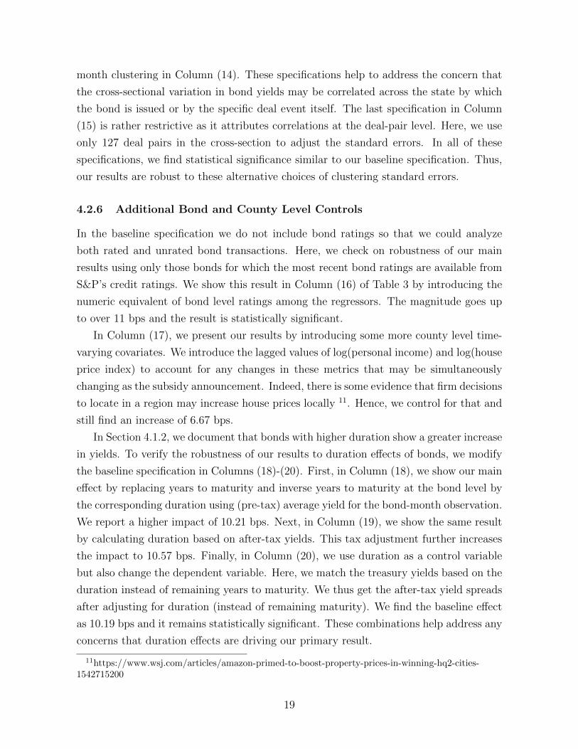
yi,c,d,t = α + β0 ∗Winneri,c,d ∗ Posti,c,t + β1 ∗Winneri,c,d + β2 ∗ Posti,c,t (1)

+BondControls+ CountyControls+ ηd + γt + εi,c,d,t

where, index i refers to bond, c refers to county, d denotes the deal pair and t indicates

the event year-month. After-tax yield spread is the dependent variable in yi,d,t obtained

from secondary market trades in local municipal bonds (described in Section 3). We also

use the raw average yield and yield spread as dependent variables. Winner corresponds

to a dummy set to one for a county that ultimately wins the subsidy deal. This dummy

equals zero for the runner-up county in that subsidy deal. Post represents a dummy that

is assigned a value of one for months after the deal is announced and zero otherwise.

The coefficient of interest is β0. The baseline specification also includes two sets of fixed

effects: deal pair fixed effects (ηd), so the comparisons are within bonds mapped to a

winner-loser pair; γt denotes year-month fixed effects to control for time trends. We

follow Bergstresser, Cohen, and Shenai (2013); Gao, Lee, and Murphy (2019a) to include

amount issued, coupon rate, dummy for status of insurance and dummy based on general

obligation versus revenue bond security type, collectively represented as BondControls.

CountyControls refers to a vector of county level measures to control for local economic

conditions. It includes the lagged value of log of labor force in the county, lagged county

unemployment rate, the percentage change in the annual labor force level and the per-

centage change in the annual unemployment rate. In all our specifications we follow

6Our results are robust to using other windows, as shown in Panel C of Table 2

7

Gao, Lee, and Murphy (2019a) in clustering standard errors at the issue-year month

level, unless specified otherwise. Our results are robust to alternate clustering methods

and reported in Section 4.2.5

Our difference-in-differences approach following Greenstone, Hornbeck, and Moretti

(2010) affords us some advantages over previously used methods in the literature. First,

we do not compare the winning counties with all other counties in the US. Such a re-

gression is likely to lead to biased estimates due to unobserved heterogeneity among the

two sets of counties. Counties that offer large subsidies could be fundamentally different

from the rest of the counties within the US. Plausibly, a county that is likely to gain

more from a particular firm locating within it is more likely to attract the project with

greater incentives. Simultaneously, a county in greater need to increase jobs is likely to

offer an aggressive incentives package. By doing so, it could try to overcome its inherent

disadvantages and influence the firms’ location decisions. These omitted factors may

also be correlated with the bond yields of the respective local issuers. By restricting

the sample to only those that were also involved in bidding for the same corporation at

the same time, we reduce the bias from such unobserved heterogeneity. To the extent

that counties may be bidding for new jobs during specific business cycles, our deals are

distributed over different periods in the 14 years during 2005-2018.

3 Data

In this section we provide details about data used in this paper. First, in Section 3.1, we

describe our data on corporate subsidies. Section 3.2 discusses the data used from the

municipal bond market. Finally, we describe some other variables used in this study in

Section 3.3.

3.1 Corporate Subsidies

The Good Jobs First Subsidy Tracker (Mattera, 2016) provides a starting point with its

compilation on establishment-level spending data. As shown in Figure IA1, states and

the federal government spent more than USD 10 billion every year in corporate subsidies

after the financial crisis of 2009. Further, there has been an increase in the portion of

subsidies offered by state governments during the sampler period of 2005-2018. States

differ in the amount of subsidy they have offered in the past with New York, Louisiana

and Michigan ranking among the top three (see Figure IA2 for a ranking among states).

On per capita basis, Washington, Oregon and Louisiana spent over USD 1,500 during this

8

period. Specifically, Figure IA3 depicts the subsidy value per capita using a chloropleth

map with five breaks shown in the legend.

One of the challenges that previous studies faced in evaluating the impact of corporate

subsidies is the lack of comprehensive data at the county-level. We discuss the literature

on location-based incentives in Internet Appendix A. The identification used in this paper

relies on close-bidding auctions where two cities compete against each other to attract a

firm. Local governments may be backed by their respective states in sponsoring money.

However, there is no published data source documenting such competing bids based on

subsidy. One contribution of our paper is to provide the first records of winning and

losing counties for large subsidy (defined as those exceeding USD 50 million) deals in the

United States. We detail the construction of the data in the Internet Appendix B.

We can identify 127 winner-loser deal pairs at the county level, which we define as

consisting our final sample with subsidy over USD 50 million in each deal7. Of these,

39 deal pairs overlap with those used in Bloom, Brynjolfsson, Foster, Jarmin, Patnaik,

Saporta-Eksten, and Van Reenen (2019). We provide a summary of the subsidy deals in

our final sample in Table 1. Panel A shows the distribution across all deals. The mean

subsidy amount in the deals is USD 300 million, whereas the median amount is USD 123

million. Comparing this to the proposed investment, we find that the median deal gets

37% subsidy as a proportion of investment. The average subsidy per job promised by

the firm amounts to nearly USD 468,000. Panel B shows that most of these deals are for

new/expansion projects with about half the deals in manufacturing (Panel C). In Table

IA3, we evaluate probable metrics in the data which may help predict the level of subsidy

offered by the winning counties. We find the investment amount and jobs promised to

be strongly correlated. Figure IA4 provides a distribution of the subsidy amounts over

different buckets. Each bin worth less than USD 500 million has at least 20 deals each.

3.2 Municipal Bonds

Municipal bond characteristics are obtained from Municipal Bonds dataset by FTSE

Russel (formerly known as Mergent MBSD). We retrieve the key bond characteristics

such as CUSIP, dated date, amount issued, size of the issue, state of the issuing authority,

name of the issuer, yield to maturity, tax status, insurance status, pre-refunding status,

type of bid, coupon rate and maturity date for bonds issued after 1990. We also use

7As such, there are 120 unique firm-year level subsidy deals among bidding states. For 6 deal-pairs,we do not have information on the jobs promised. There were 13 pairs for which we could not gatherdata on the size of investment for the proposed project.

9

S&P credit ratings for these bonds by reconstructing the time-series of the most recent

ratings from the history of CUSIP-level rating changes. We encode character ratings

into numerically equivalent values ranging from 28 for the highest quality and 1 for the

lowest.

An important step in our data construction is to link the bonds issued at the local

level to the counties which make the subsidy bids. This geographic mapping would allow

us to study the implications on other economic variables using data on demographics and

county-level financial metrics. Since the FTSE Municipal Bonds dataset does not have the

county name of each bond, we need to supplement this information from other sources like

Bloomberg. However, in light of Bloomberg’s download limit, it is not feasible to search

information on each CUSIP individually. Therefore, we first extract the first 6 digits of

the CUSIP to arrive at the issuer’s identity8. Out of 63,754 unique issuer identity (6-digit

CUSIPs), Bloomberg provides us with county-state names on 59,901 issuers. For these

issuers, we match the Federal Information Processing Standards (FIPS) code. The FIPS

is then used as the matching key between bonds and bidding counties involved in offering

corporate subsidies. We also match the names of issuers to the type of (issuer) government

(state, city, county, other) on Electronic Municipal Market Access (EMMA) provided by

Municipal Securities Rulemaking Board. We use this information to distinguish local

bonds from state level bonds because we are interested in the non-state bonds.

We use Municipal Securities Rulemaking Board (MSRB) database on secondary mar-

ket transactions during 2005-2018. Our paper closely follows Gao, Lee, and Murphy

(2019a) in aggregating the volume-weighted trades to a monthly level. Following Down-

ing and Zhang (2004); Gao et al. (2019b), we only use customer buy trades to eliminate

the possibility of bid-ask bounce effects. Table IA4 summarizes each step of the sam-

ple construction (Schwert, 2017). Given our primary focus on the borrowing cost from

secondary market yields, our sample is derived from the joint overlap between the bond

characteristics and bond trades at the CUSIP level. In matching the bond transactions

from secondary market data to their respective issuance characteristics (from FTSE Rus-

sell), we rely on the CUSIP as the key identifier. In Table IA5, we provide descriptive

statistics on bond features pertaining to the primary market and secondary market, re-

spectively. We provide the description of key variables in Table A1.

The primary outcome variable used in Equation 1 is the tax-adjusted spread over

risk free rate. We match the bond’s remaining maturity to that of zero coupon yields

8The 9-digit CUSIP consists of the first six characters representing the base that identifies the bondissuer. The seventh and eighth digits identify the type of the bond or the issue. The ninth digit is acheck digit that is generated automatically.

10

to get the reference benchmark for risk free rate following Gurkaynak, Sack, and Wright

(2007). Tax adjustment follows Schwert (2017) wherein marginal tax rate impounded in

the tax-exempt bond yields is assumed to be the top statutory income tax rate in each

state. This is consistent with the broad base of high net worth individuals and households

who form a major section of investors in the US municipal bond market (often through

mutual funds even). A detailed study on tax segmentation across states by Pirinsky and

Wang (2011) shows significant costs on both issuers and investors in the form of higher

yields. In particular, we use:

1 − τs,t = (1 − τ fedt ) ∗ (1 − τ states,t ) (2)

To compute the tax-adjusted spread on secondary market yields:

spreadi,t =yi,t

(1 − τs,t)− rt, (3)

where rt corresponds to the maturity matched zero coupon yield for a bond traded at

time t. From Schwert (2017), we use the top federal income tax rate as 35% during 2005

to 2012, and 39.6% for 2013 to 2015. Extending the last segment further, we use the

same rate for 2016 as well. Subsequently, we match the municipal bond yields to similar

maturity zero coupon yields (ZCY) to get the corresponding proxy for risk free rates. We

round the bond maturity in years to the nearest integer. Since ZCY is not available for

maturity over 30 years, we can not match those bond observations with risk free rate and

they do not feature in the final analysis. However, since the average remaining maturity

for the sample is 10 years, this should not create a significant bias.

3.3 Other Variables

We use Census data from the Census Bureau Annual Survey of Local Government Fi-

nances to get details on revenue, property tax, expenditures and indebtedness of the local

bodies. This gives us detailed constituents of revenue and tax components at the local

level, which we use in additional tests to examine the implications for our main results.

We use county level household income from Internal Revenue Service (IRS) to get total

personal income at the county level. Our unemployment data comes from Bureau of La-

bor Statistics. For county-level population, we use data from Surveillance, Epidemiology,

and End Results (SEER) Program under the National Cancer Institute. As a proxy for

risk free rate, we use zero coupon yield provided by FEDS, which provides continuously

compounded yields for maturities up to 30 years. To get tax-adjusted yield spreads, we

11

use the highest income tax bracket for the corresponding state of the bond issuer from

the Federation of Tax Administrators.

4 Results

We discuss our baseline results (Section 4.1) for Equation 1, including evidence from

the dynamics from the raw data on yields, evidence on parallel trends assumption and

a falsification test. Section 4.2 shows robustness tests for our baseline specification. We

propose the potential mechanism to explain our results in Section 4.3. In Section 4.4,

we analyze the heterogeneity in relative bargaining power between the county and the

firm involved in the subsidy deal. Finally, we discuss the impact on primary market of

municipal bonds (Section 4.5) and local property taxes and public expenditure (Section

4.6).

4.1 Impact on Borrowing Costs of Local Governments

4.1.1 Dynamics and Baseline Results

We begin our analysis by plotting the yields observed in the secondary market between

the winning and losing counties. Our event window comprises three years before and

after the subsidy deal announcement. We use the 12 months before the event window

(T=-37 to T=-48 months) as the benchmark period to evaluate the pre-trends between

the treatment and control groups. We depict the observations aggregated to a quarterly

scale to mitigate the inherent limitations of liquidity in the municipal bond market. We

plot the raw yields based on Equation 4 below.

yi,c,d,t = α + βq ∗q=12∑q=−12

Winneri,c,q ∗ Posti,c,q + δq ∗q=12∑q=−12

Loseri,c,q ∗ Posti,c,q (4)

+ ηd + κt + εi,c,d,t

where, index i refers to bond, c refers to county, d denotes the deal pair, t indicates

the event year-month and q refers to the quarter corresponding to the event month t.

After-tax yield spread is the dependent variable in yi,c,d,t obtained from secondary market

trades in local municipal bonds. ηd represents the deal-pair fixed effects; κt represents the

year-month fixed effects. The coefficients βq and δq represent the average change in yields

with respect to the benchmark period for the winning and losing counties, respectively.

In Figure 1a, the solid line with circles plots the pre-tax average yield over the 3-year

12

window for winning counties on average. The losing counties are depicted using a dashed

line with diamonds. The figure reveals no statistical difference between the two groups

before the deal announcement. The treatment and control groups exhibit parallel trends

in terms of bond yields. Second, the average yields for the winning counties appears to be

higher than that of the losing counties in the first quarter after the deal. Finally, we find

that the difference between the two groups persists for at least 10 quarters. The trends

look similar for yield spread as the dependent variable (Figure 1b). Consistent with

Schwert (2017), we adjust the yield and yield spread for taxes because many municipal

bonds are tax-exempt securities. We find similar results for after-tax yield and after-tax

yield spread (Figures 1c and 1d) as our dependent variable. We use the after-tax yield

spread as our primary dependent variable in the subsequent analysis.

Note that the above results only represent the raw difference in yields between the

two groups by stacking the 127 deal-pairs in our sample into an aggregated set. These

findings do not control for differences in bond characteristics and local economic condi-

tions over time. Next, we estimate our difference-in-differences using our baseline Equa-

tion 1. Here, the coefficient β0 of the interaction term, Winneri,d * Posti,t, identifies

the differential effect after the subsidy deal announcement on average yields of winning

counties in comparison to the losing counties where we control for observable character-

istics. To revisit our identifying assumption: the losing county serves as an adequate

counterfactual to map how the winner’s yields would have changed in the absence of the

deal announcement. The deal fixed effects ensure estimation from within each deal pair.

The year-month fixed effects control for declining yields in the overall municipal market

during our sample period, over and above the treasury adjustment for spreads.

Table 2, Panel A reports the effect of winning a subsidy deal on the municipal bond

yields using Equation 1. In Column (1) - Column (3), we estimate the regression equation

using the raw average yield as the dependent variable. Specifically, Column (1) denotes

the estimates without using any controls. We use bond level controls in Column (2),

which consist of coupon (%), log(amount issued in USD), dummies for callable bonds,

additional credit enhancement, general obligation bond and competitively issued bonds,

remaining years to maturity and inverse years to maturity. We provide the description

of key variables in Table A1. In Column (3), we control for the county-level variation

in unemployment rate and labor force. We use the lagged values (to the year of deal

announcement) for log(labor force) and unemployment rate, and the percentage change

in unemployment rate and labor force, respectively. Since subsidies are often motivated

by job creation, we use these measures at the county level consistent with previous

13

literature.9 Thereafter, in each successive triplet of columns, we follow the same scheme

and show our results using yield spread as a dependent variable, followed by after-tax

yield spread.

Using Column (9) of after-tax yield spread as our baseline case implies that the yield

spread for winning counties increases by 8.36 bps after the subsidy announcement, in

comparison to the losing counties. The 8.36 bps is equivalent to additional borrowing

cost amounting to 7.5% (=2.8/38) of the total subsidy ($38 billion) offered during the

sample period. To arrive at this magnitude, we start with the outstanding municipal

debt of the winning counties. We find that this amount is ∼ $400 billion in the deal year.

The increase of 8.36 bps amounts to $334 million (=0.000836*400*1,000) in additional

interest costs per annum. The average outstanding maturity of bonds is 10 years. We

discount this additional monetary cost for 10 years using the average yield (winners) of

2.8% to get $2.8 billion.

Next, in Panel B we show the baseline result of Column (9) using different forward

windows, keeping the pre-event window same as three years. We find that the magnitude

of the differential impact increases from about 5 bps within the first six months after

the event (Column (1)) to about 12 bps in 5 years (Column(8)). There seems to be a

gradual increase in magnitude which likely persists beyond the immediate near-term. To

evaluate the sensitivity of our results against the choice of window used, we show our main

result in Panel C using different pre- and post-windows. While the effect is relatively

small in magnitude and weak in significance for the 12 month window in Column (1), we

see qualitatively similar results for other windows in the remaining columns. We argue

that a longer period is needed both in the preceding and succeeding periods around the

announcement to arrive at sharper estimates of the effect, especially given the limited

trading in the municipal bond market. We also observe an increase in trading activity

after the deal announcement. We find an increase in both customer buy and customer

sell trades and report results in Table IA8. In the next sub-section, we provide evidence

on the parallel trends assumption.

4.1.2 Do bond yields respond to underlying local economic differences?

Our baseline comparison between winning and losing counties’ yields assumes similar

local economic conditions between the treatment and control groups during the event

window around the deal. The results in Section 4.1 suggests that winning and losing

9We report these coefficients for bond level and county level controls in Table IA7. For robustness,we further include the lagged values of log(personal income) and log(house price index). The magnitudeof our main effect remains similar reported in Section 4.2

14

counties exhibit parallel trends in their bond yields. However, as discussed before, the

decision by local governments to engage in the bidding process to attract firms may

not be random. Thee local administration may be attempting to create new jobs or to

retain existing ones by offering incentives. It could be the case that bondholders from

these counties are responding to underlying differences between the winning and losing

counties. We test such underlying economic differences based on some relevant observable

economic indicators. We present the comparison of the average trends at the county-level

in a) aggregate employment, b) unemployment rate, c) S&P municipal bond rating and

d) local beta between winners and losers in Figure IA5. In each of these subplots we

use the annualized version of Equation 4, but additionally introduce county fixed effects.

Here, we cluster standard errors at the deal level.

In Figures IA5a and IA5b, we find that the aggregate employment shows an upward

trend while the unemployment rate decreases. Both winning and losing counties seem

to follow a similar trajectory with no statistical difference between them. This supports

our parallel trends assumption on these key metrics related to employment. However, it

is worth noting that after the subsidy deal, the increase in employment in the winning

county is similar to that in the losing county.

Further, Figures IA5c and IA5d provide a comparison of the county level credit-

worthiness and riskiness, respectively. We use bond level ratings aggregated up to the

event-year to get the county level ratings. As shown in the figure, the two groups do not

show any difference in trends. Since the rating of the winners is not worse than that of

the losers, this also helps against the concern of negative selection. Finally, the local beta

is a measure defined in Tuzel and Zhang (2017). Using this as a proxy for the underlying

riskiness of the counties, we find that both winning and losing counties had similar local

beta during the event window. Overall, the results suggest that the winning and losing

counties look similar based on local economic conditions during the event period.

Next, we estimate a multivariate linear probability model to understand if the local

economic factors jointly determine the probability of winning a deal by the county. We

use the local conditions during the 3 years before the deal as the regressors. In addition

to using the four control variables in our baseline specification on unemployment and

labor force, we further introduce the median income and house price index. Table IA9

shows the regression results where we introduce each regressor successively. We plot the

coefficients from Column (6) in Figure IA6 and show the confidence intervals at the 95%

level. For each metric on the y-axis, we show the explanatory power in determining

the ‘winner’ dummy. We find that the coefficient for none of these key local metrics

significantly differs from zero.

15

Another potential concern in our identification is about the timing of the subsidy

announcement. In our baseline specification, we use county level controls to absorb vari-

ation in key economic metrics that may be relevant to the subsidy offer. But it does

not control for unobserved time-varying county specific changes that may be happening

simultaneously as the deal is announced, which may also affect the bond yields. More-

over, local government officials may be responding to undisclosed information about the

county’s health with the incentive deal. If bondholders are also privy to such private

information that may weaken our main result. However, if this is the case, we should

observe increase in yields for all types of bonds irrespective of use of proceeds. We find

that not all types of municipal bonds demonstrate a change in yields as shown in Figure

IA7. The effect is primarily driven by bonds raised to finance primary education (5.11

bps), economic development (7.06 bps) and infrastructure (21.19 bps). In fact, the neg-

ative effect on other public services (-5.24 bps) and water-sewer (-8.33 bps) shows that

the results are not driven by the declining health of the winning county. Consistently,

we also find that bonds with longer duration show a higher increase in yields. For exam-

ple, bonds with duration less than 5 years do not seem to get affected. There is a 7.11

bps increase in bonds with duration of 5-10 year and 12.44 bps increase for bonds with

duration over 10 years.

4.1.3 Falsification Tests: Pre-Refunded Bonds

It is common for municipal bond issuers to pre-refund bonds before the call date by

issuing new debt and holding the proceeds in a trust to fund remaining payments until

the call date. This would effectively render the pre-refunded bonds risk free (Fischer,

1983; Chalmers, 1998; Schwert, 2017). Local governments may choose to pre-refund their

bonds thereby offering a clean change of the said bonds from risky to risk-free. We exploit

this argument to claim that bonds which have been thus “insured” would not see any

significant change in their yields in our setting of Equation 1.

To construct the sample of pre-refunded bonds for this test, we follow Ang, Green,

Longstaff, and Xing (2017) and Schwert (2017). We apply the following filters to our

sample: keep only the pre-refunded bonds, exclude bonds that are not exempt from

federal within-state income taxes; exclude pre-refunded bonds that are not escrowed by

Treasury securities, State and Local Government Series (SLGS), or cash. Finally, we

exclude bonds that are pre-refunded within 90 days of the call date since the Internal

Revenue Service treats these transactions as different from pre-refunding, called current

refunding. Table IA6 shows the results of the falsification test. In Column (1), we find

that the average yield for winners goes up by a marginally small magnitude of about

16

1.5 bps, but the measure is not statistically significant. Likewise, in Column (2), we do

not find any significant change to the yield spread as the outcome variable among the

pre-refunded bonds. Finally, Columns (3) and (4) report the effect on after-tax yield

spreads without and with county controls, respectively. The magnitude is even smaller

than the previous two columns and statistically insignificant again. Thus, we do not find

any impact on these pre-refunded bonds as they have been secured against the escrow of

funds deemed for their outstanding payments. The absence of any marginal impact in

the subset of pre-refunded bonds suggests that our main effect is not driven by overall

market conditions in the US municipal market.

4.2 Robustness Tests

In this section, we test the robustness of our main result in Column (9) of Table 2 to

various alternative specifications. We present the results of these robustness checks in

Table 3.

4.2.1 Is the effect driven by large institutional trades?

In 2018, about USD 0.96 trillion out of USD 3.25 trillion of the municipal bond holdings

was managed by money market mutual funds and exchange-traded funds. One poten-

tial concern is that few large institutional trades may be driving our main result. We

separate our results into sub-samples of trades constituting various buckets. Retail-sized

transactions usually correspond to $ 100,000 or less 10. Column (1)-(3) depict the main

effect from Equation 1, as derived from trade sizes worth ≤ $25,000, ≤ $50,000 and ≤$100,000. The increase in borrowing cost is over 9 bps in each of these sub-samples. This

suggests that our main result is also present in smaller transactions.

4.2.2 Are results driven by newly issued bonds?

Even though our data from MSRB on secondary market bond yields is cleaned for

primary-market transactions recorded therein, we assume further precaution in favor

of seasoned bonds. In Columns (4)-(7), we report our baseline results by dropping bonds

that were recently issued i.e., within 6, 12, 24 and 36 months of the subsidy announce-

ments. By doing so, we remove bonds from the sample that have been newly issued and

may demonstrate unusual trading in the initial phases. The magnitude ranges from 7.46

to 5.01 bps, which is lower than our baseline case, but still statistically and economically

10http://www.msrb.org/~/media/Files/Resources/Mark-Up-Disclosure-and-Trading.ashx?

17

significant. This shows that our results are not only driven by trading activity in newly

issued bonds.

4.2.3 Financial Crisis of 2009

Another potential worry may be due to the sample period spanning the financial crisis

of 2009. Understandably, this was a period of major volatility in the financial markets

across asset classes and municipal bonds were not immune to this. As a result, we report

our findings by excluding this period from our data. We consider two approaches: first,

in Column (8), we show our results by only keeping bond transactions after 2009. This

reduces the number of observations and the magnitude goes down to 5.83 bps. Second, in

Column (9), we show the results by retaining only those deal events that were announced

after 2009. In this case, the borrowing cost increases by 8 bps. Taken together, we argue

that our regression estimates in the baseline specification are not entirely driven by

unusual activity in the municipal bond market due to the financial crisis of 2008-09.

4.2.4 Other Trades

In our baseline estimates, we use only customer buy trades at the local level. We test

our specification using a different set of trades/bonds in our baseline. First, to evaluate

if our results are sensitive to the choice of customer-buy trades, we run the baseline

regression using only the customer-sell trades (Column (10)). There is still an increase

of about 6 bps. Second, in Column (11), we document the impact on state level bonds

only (otherwise excluded from our main sample) among the bidding states. As expected,

the impact is much lower (1.39 bps) at the state-level as the primary impact of many of

the corporate subsidy deals is at the local county level.

4.2.5 Assumptions on correlation of standard errors

In our baseline specification, we cluster standard errors by issue-year month following

Gao, Lee, and Murphy (2019a,b). In Columns (12)-(15), we show our main result using

alternative definitions for clustering. First, we consider the possibility that the standard

errors may be correlated across different bond issuers over the calendar months (see

Column (12)). Further, it could also be that the error term in our main specification

is correlated over specific bond issues and over event months (instead of year month),

i.e. relative to the subsidy announcement date. This accounts for the fact that the bond

market response may be sharper and correlated in the first few months just after the

news of the deal. We also use state-year month clustering in Column (13) and deal-year

18

month clustering in Column (14). These specifications help to address the concern that

the cross-sectional variation in bond yields may be correlated across the state by which

the bond is issued or by the specific deal event itself. The last specification in Column

(15) is rather restrictive as it attributes correlations at the deal-pair level. Here, we use

only 127 deal pairs in the cross-section to adjust the standard errors. In all of these

specifications, we find statistical significance similar to our baseline specification. Thus,

our results are robust to these alternative choices of clustering standard errors.

4.2.6 Additional Bond and County Level Controls

In the baseline specification we do not include bond ratings so that we could analyze

both rated and unrated bond transactions. Here, we check on robustness of our main

results using only those bonds for which the most recent bond ratings are available from

S&P’s credit ratings. We show this result in Column (16) of Table 3 by introducing the

numeric equivalent of bond level ratings among the regressors. The magnitude goes up

to over 11 bps and the result is statistically significant.

In Column (17), we present our results by introducing some more county level time-

varying covariates. We introduce the lagged values of log(personal income) and log(house

price index) to account for any changes in these metrics that may be simultaneously

changing as the subsidy announcement. Indeed, there is some evidence that firm decisions

to locate in a region may increase house prices locally 11. Hence, we control for that and

still find an increase of 6.67 bps.

In Section 4.1.2, we document that bonds with higher duration show a greater increase

in yields. To verify the robustness of our results to duration effects of bonds, we modify

the baseline specification in Columns (18)-(20). First, in Column (18), we show our main

effect by replacing years to maturity and inverse years to maturity at the bond level by

the corresponding duration using (pre-tax) average yield for the bond-month observation.

We report a higher impact of 10.21 bps. Next, in Column (19), we show the same result

by calculating duration based on after-tax yields. This tax adjustment further increases

the impact to 10.57 bps. Finally, in Column (20), we use duration as a control variable

but also change the dependent variable. Here, we match the treasury yields based on the

duration instead of remaining years to maturity. We thus get the after-tax yield spreads

after adjusting for duration (instead of remaining maturity). We find the baseline effect

as 10.19 bps and it remains statistically significant. These combinations help address any

concerns that duration effects are driving our primary result.

11https://www.wsj.com/articles/amazon-primed-to-boost-property-prices-in-winning-hq2-cities-1542715200

19

4.2.7 Unobserved heterogeneity at county and state levels

Our baseline specification controls for relevant time-varying county-level observables. We

now consider whether our results are robust to a host of unobserved factors at the county

and state level. First, we absorb all county level, time-invariant variation beyond the deal

fixed effects in Column (21). This yields a baseline effect of 10.54 bps. Next, we impose

county-year fixed effects to absorb county-level variation that changes over calendar years.

In Column (22), we report an increase of 2.87 bps which is statistically significant at the

1% level. Given the buy and hold nature of the investors in this market, we argue that

this is a very restrictive setting. This results in a substantially muted effect. Next, in

Column (23) we show the result by dropping counties that may get repeated as a winner

or a loser within 6 years of the previous deal. Here, the number of observations reduces

substantially but even so the magnitude increases to 13.42 bps. Next, to control for state

level characteristics among the bidding counties, we show our results with state fixed

effects and state-year fixed effects in Columns (24) and (25) respectively. This may be

relevant because the competition often manifests at the level of the state governments.

We find a significant impact even though the magnitude drops to 3.16 bps in Column

(25). Overall, our results suggest that time-varying unobservables at county and state

levels may not be the primary driver of our main results.

4.2.8 Alternative specifications

Finally, we also consider some other specifications. We start with a very restrictive

specification in Column (26) where we impose bond fixed effects. We also require that

the same bond was trading at least once before and after the announcement of subsidy.

These requirements are over and above the baseline specification which seeks to tease out

variation between winning county and losing county from within a deal pair. Here, the

magnitude drops to about 4 bps, but is still significant. We argue that this bond-specific

impact may not represent the average borrowing cost prevailing for the overall county

in the secondary market. Thus, it is an under-estimation of the main effect and may

correspond to the lower-bound.

Next, we address the concern that the relative age of the transaction with the respect

to the deal announcement may vary over time. We introduce event month fixed effects

over and above the year-month fixed effects in Column (27). The magnitude remains

similar to our baseline case. Next, in Column (28) we replace the year-month fixed

effects with event-month fixed effects. Our magnitude goes up to 9.31 bps, thereby

indicating that our choice of using the year month fixed effects is more conservative.

20

In Column (29), we use the event month fixed effects as in the Column (28), but now

cluster the standard errors by issue-event month. Our results are still robust to this

choice of clustering for the alternative specification in fixed effects. In Column (30), we

replace the month fixed effects with calendar year fixed effects and find that a higher

magnitude of 11.25 bps for our key variable. This again reinforces our rationale to use

the more conservative year month fixed effects in the baseline specification to absorb for

month-specific variation over and above the year-specific variation.

4.3 Mechanism

As we discussed before, the local governments face a trade-off while using targeted busi-

ness incentives i.e., foregoing future tax revenue versus anticipated jobs multiplier benefit

(see Greenstone and Moretti (2004)). The increased demand for public services after the

new plant opening while simultaneously foregoing revenue in the form of subsidy may

require local governments to increase municipal debt. The underlying debt capacity of

the winning counties may impact the cost of existing debt and additional borrowing.

Whereas, the large multiplier effect of new plant on incumbent businesses may attenuate

the effect of debt capacity. In this section, we discuss the effect of debt capacity on

municipal borrowing cost and its interaction with the expected multiplier effects.

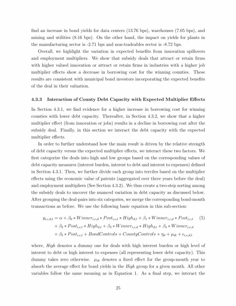
4.3.1 County Debt Capacity

We consider ex-ante debt capacity of local governments using three proxies: a) interest

expenditure, b) county credit ratings, and c) tax privilege. First, we expect the secondary

market impact to be higher for winning counties with large ex-ante interest expenditure.

To this end, we use three measures based on the ex-ante interest expenditure, namely:

(i) interest burden (ratio of interest on general debt to total revenue), (ii) interest to debt

(ratio of interest on general debt to total long term debt outstanding) and (iii) interest

to expenses (ratio of interest on general debt to total expenditure). We use interest in

the year preceding the deal, scaled by the corresponding fiscal metric two years before

the deal. A high value of the interest expenditure measure corresponds to a low debt

capacity.

We divide the winning counties into two bins based on the median of the interest

expenditure measures (as defined above). Using our baseline Equation 1 with interactions

for the bins, we estimate the differential impact on high versus low debt capacity counties.

We also include group-month fixed effects in the regression. The results are depicted in

Figure 2 which shows the coefficient of interaction term for each group. First, among

21

counties with high interest burden ratio, we find the bond yields going up by 15.34 bps.

This corresponds to the higher debt burden these counties face since more of their revenue

is devoted to meeting general debt interest costs. Similarly, in the next bar graphs, we

find that the borrowing cost for counties with higher ex-ante interest to debt ratio goes

up by 22.13 bps. In contrast, counties with low interest to debt see a reduction in yields

of about 8.93 bps. The difference between the two groups is economically and statistically

significant. We find similar results by using interest to expense ratio.

Next, we consider debt capacity using county credit ratings. Table 4 shows the

results for our analysis. We interact our baseline Equation 1 with dummy variables

corresponding to ex-ante high credit rating versus low credit rating winning counties12.

As before, we control for the average effect within a group in a given month using the

relevant fixed effects. Our estimation results show that a lower credit rating is associated

with a higher increase in the winning county’s municipal bond yields. In Column (1),

we show the results corresponding to all bonds (with a rating) in our sample. We find

an increase of 8.45 bps for counties rated as A+ and below; whereas, the increase in

yields is 5.89 bps for counties rated as AA- and above. Similarly, within the subset of

general obligation bonds, the yields go up by 16.69 bps among the low rated counties. On

the other hand, the yields decrease by 6.74 bps for high rated counties. The difference

between the two groups is economically and statistically significant. Column (3) shows

the results corresponding to the subset of revenue bonds, which are qualitatively similar

to the full sample results of Column (1).

Finally, drawing upon the demand side of municipal bonds, we explore the debt

capacity of the county with respect to the local investor base. This argument is based

on the retail clientele/ownership for municipal bonds, the local home biasand the unique

tax-exemption from investment into this market. These features support the idea that

if a county has many potential subscribers to local bonds, then it should have a higher

debt capacity. As a result it should find better cushion against adverse shocks to its

bond prices. To test this, we adapt the tax privilege measure in Babina, Jotikasthira,

Lundblad, and Ramadorai (2019). It is defined as the highest state income tax rate

applied to income from municipal bonds issued by other states minus the highest state

income tax rate applied to income from the winning state-issued municipal bonds. Since

12The county level credit rating is based on the average S&P rating for the corresponding bonds asobtained from MBSD. To use a clean period before the event, we focus on ratings during 12 to 24months prior to the deal month. Here, our subset of general obligation bonds is obtained by specificallyusing“Unlimited Tax GO” bonds. All others are classified as revenue bonds. We separately obtaincounty level rating corresponding to all bonds, general obligation bonds only and revenue bonds bondsonly respectively.

22

different states in the US have different state level tax rates, it creates a distortion in the

incentives to buy/hold municipal bonds. States with lower tax privileges are more likely

to have a smaller investor base.

In Table 5, we document the variation among different terciles of tax privilege among

the winning counties. We use the baseline specification from Equation 1, after control-

ling for average group-month effects. Column (1) shows the results for the full sample

where we find a 21.61 bps increase for the lowest tercile, alongside a contrasting 19.49

bps decline in yields for the highest group. Column (2) shows a similar effect for tax-

exempt bonds. Consistent with Babina, Jotikasthira, Lundblad, and Ramadorai (2019),

we further control our baseline specification with the lagged values of debt-to-income at

the county level. We obtain the county level total personal income from the Internal

Revenue Service data. We show our results in Column (3) with magnitudes being sim-

ilar to the previous two columns. Finally, we use a measure of tax privilege gap as the

difference in tax privilege between the winning and losing counties. Following a similar

scheme, we show the results in Columns (4) - (6). Once again, the low tax incentive

winners experience a much larger increase in borrowing costs than their medium-placed

counterparts. For winners in the high tax privilege bracket, there is a reduction in yields

by 8-19 bps. The evidence supports that a low debt capacity measured by a low tax

privilege results in a greater increase in bond yields.

To summarize, our results in this subsection provide evidence in favor of the ex-ante

debt capacity of winners as the underlying channel. We show that winning counties which

face a higher interest burden are associated with up to 21 bps as additional borrowing

cost. Similarly, low rated counties also pay more for their debt after the deal. Finally,

a lower tax privilege reflects lower debt capacity for a county resulting in up to 27 bps

increase in bond yields.

4.3.2 Expected Multiplier Effects

In this sub-section we evaluate the heterogeneity in potential benefits after the subsidy

deal. As noted before, a direct assessment of the future economic impact of the subsidies

on the local community is challenging. Most of these projects have a long gestation period

and the benefits get realized over a longer horizon. We hypothesize that the municipal

bond prices reflect the expected local benefit from the subsidy deal. We measure the

expected multiplier effects using two proxies: a) knowledge spillover using firm patents,

and b) national industry-specific jobs multiplier.

First, to measure knowledge spillover, we follow Kogan, Papanikolaou, Seru, and

Stoffman (2017) to quantify the economic importance of each patent of the firm receiving

23

the subsidy. Specifically, we use the dollar value of innovation associated with the firm

receiving the subsidy. We aggregate this value over patents granted three (and five) years

before the deal13. We create three equal terciles among winners in the matched deals.

Using our baseline Equation 1 interacted with the corresponding group of the tercile, we

get the results as depicted in Figure 3a. We also control for group-month fixed effects. By

aggregating up to three years before the deal, we find an increase in yields of 16.83 bps

among deals involving firms with the lowest tercile of patent value. On the other hand,

the borrowing cost seems to go down in deals involving firms with the highest tercile of

patent value. The difference between these two extremes of 19.31 bps is economically and

statistically significant. Further, we find a similar impact when we use a longer history of

the firms and aggregate the value of patents up to five years before the deal. The lowest

group shows a statistically significant increase in yields of 14.71 bps, while the yields

drop significantly by 5.06 bps among the high patent values. Once again, the difference

of 19.77 bps is statistically and economically significant. Taken together, the evidence

suggests that the borrowing cost decreases for deals involving high innovation/patent

value (see Moretti (2012)).

The economic benefit reported in the press releases of many subsidy deals includes the

prospect of many indirect jobs getting created. Proponents of corporate subsidy often

refer to this multiplicative effect on jobs created in the value chain of a given industry

(based on upstream or downstream linkages). As a result, we consider the variation

across deals based on the jobs multiplier associated with a given industry. For this, we

hand match the industry (and/or project description) of the 127 deals in our sample to

employment multipliers by industry provided by the Economic Policy Institute14. We

divide the winners of the subsidy deals into terciles based on the employment multipliers

associated with the industry of the firm. Then, we use our baseline Equation 1 interacted

with the corresponding group. We also control for group-month fixed effects. Figure 3b

shows the differential effect across the three groups. Among deals in the lowest tercile,

the impact is highest: borrowing cost goes up by 7.01 bps. The effect diminishes to 3.12

bps and 1.71 bps in the medium and high jobs multiplier groups. The difference between

the impact on the lowest and the highest terciles is 5.30 bps. This statistically significant

result points toward the economic interpretation of smaller increase in the borrowing

cost after the subsidy deal if the expected employment multiplier for the deal is higher.

Further, we find variation at the industry level of the deal, as reported in Figure 3c. We

13We are able to match 60 deal-pairs in our subsidy database to the patents granted until 2010. Fordeals which can be linked to the patent-CRSP (firm) database but do not have any patents associatedwith them, we assign their value of innovation as zero.

14https://www.epi.org/publication/updated-employment-multipliers-for-the-u-s-economy/

24

find an increase in bond yields for data centers (13.76 bps), warehouses (7.05 bps), and

mining and utilities (8.16 bps). On the other hand, the impact on yields for plants in

the manufacturing sector is -2.71 bps and non-tradeables sector is -8.72 bps.

Overall, we highlight the variation in expected benefits from innovation spillovers

and employment multipliers. We show that subsidy deals that attract or retain firms

with higher valued innovation or attract or retain firms in industries with a higher job

multiplier effects show a decrease in borrowing cost for the winning counties. These

results are consistent with municipal bond investors incorporating the expected benefits

of the deal in their valuation.

4.3.3 Interaction of County Debt Capacity with Expected Multiplier Effects

In Section 4.3.1, we find evidence for a higher increase in borrowing cost for winning

counties with lower debt capacity. Thereafter, in Section 4.3.2, we show that a higher

multiplier effect (from innovation or jobs) results in a decline in borrowing cost after the

subsidy deal. Finally, in this section we interact the debt capacity with the expected

multiplier effects.

In order to further understand how the main result is driven by the relative strength

of debt capacity versus the expected multiplier effects, we interact these two factors. We

first categorize the deals into high and low groups based on the corresponding values of

debt capacity measures (interest burden, interest to debt and interest to expenses) defined

in Section 4.3.1. Then, we further divide each group into terciles based on the multiplier

effects using the economic value of patents (aggregated over three years before the deal)

and employment multipliers (See Section 4.3.2). We thus create a two-step sorting among

the subsidy deals to uncover the nuanced variation in debt capacity as discussed below.

After grouping the deal-pairs into six categories, we merge the corresponding bond-month

transactions as before. We use the following basic equation in this sub-section:

yi,c,d,t = α + β0 ∗Winneri,c,d ∗ Posti,c,t ∗Highd,t + β1 ∗Winneri,c,d ∗ Posti,c,t (5)

+ β2 ∗ Posti,c,t ∗Highd,t + β3 ∗Winneri,c,d ∗Highd,t + β4 ∗Winneri,c,d

+ β5 ∗ Posti,c,t +BondControls+ CountyControls+ ηd + µdt + εi,c,d,t

where, High denotes a dummy one for deals with high interest burden or high level of

interest to debt or high interest to expenses (all representing lower debt capacity). This

dummy takes zero otherwise. µdt denotes a fixed effect for the group-month year to

absorb the average effect for bond yields in the High group for a given month. All other

variables follow the same meaning as in Equation 1. As a final step, we interact the

25

equation above with corresponding dummies at the deal level pertaining to terciles in

value of patents and employment multipliers. We suitably modify µdt to control for the

average effect of the tercile sub-group in a given month.

In Figure 4a, we show how debt capacity interacts with knowledge spillover. For

example, using interest burden, we find that the differential effect of high interest burden

is muted due to a high value of patents (-0.04 bps). We find similar results using other

measures of debt capacity, like interest to debt and interest to expenses. Next, we

interact the debt capacity with jobs multiplier. We find similar results. We show that

the marginal impact of high interest burden is significantly reduced for deals with high

jobs multiplier (-7.87 bps). Our results show similar effect with other measures using

interest to debt and interest to expenses.

Taken together, our results in Section 4.3 suggest that lower debt capacity increases

the impact on borrowing cost. Whereas, expected multiplier attenuates this impact. Fur-

ther, the interaction of debt capacity with expected multiplier suggests that the potential

gains from knowledge spillover and expected jobs may help mitigate the negative effects

of debt capacity.

4.4 Bargaining Power: County versus Firm

So far, we have considered the impact of the debt capacity of the county and potential

multiplier effects of the deal on the municipal bond yields. But, the amount of subsidy

given to attract or retain firms to the county relative to the projected benefits is likely

to be a major factor in the price reaction to the deal. The offered subsidy is in turn

likely to depend on the relative bargaining power between the parties involved in the

subsidy deal. We argue that while firms may hire site consultants to conduct their

search through a bidding mechanism15, local governments may not have access to such

sophisticated resources. To assess the relative bargaining power between the county and

the firm, we use the following: a) ratio of firm’s assets to county’s revenue, b) ratio of

subsidy to county’s budget surplus, c) intensity of bidding competition, and d) county’s

unemployment rate.

First, we divide the winning counties based on the ratio of firm assets to county-level

revenue. We hypothesize that if the firm (size represented by assets) is larger than the

county (size represented by revenue), then the county’s relative bargaining power is likely

to be lower. Therefore, the impact on borrowing cost would be higher. In Column (1) of

15For instance, The Wall Street Journal reported on a cadre of consultants which help companies decidethe location of their projects: https://www.wsj.com/articles/meet-the-fixers-pitting-states-against-each-other-to-win-tax-breaks-for-new-factories-11558152005

26

Table 6, we report our results for the baseline Equation 1 interacted with terciles of this

measure. We also control for group-year month fixed effects. We find that yields go up

by 14.52 bps for deals with high firm assets to county revenue ratio. On the other hand,

the yields actually decrease by 4.5 bps when this ratio is low. The difference between

the two sub-groups is significant. We find similar impact by using our second measure of

subsidy to county budget surplus ratio. As shown in Column (2), the cost increases by

19.37 bps for the high group, but decreases by 11.53 bps when the corresponding ratio

is low.

Since the competition for these firm investments is often supported by the state level

governments, we construct our next measure at the state level. We calculate the ratio

of state level budget surplus to revenue and use the gap between the winning and losing

state as a measure of intensity of competition. As the gap between states increases,

the competition is likely to be lower and the county’s bargaining power is likely to be

higher. In Column (3), we show our results based on the interaction with intensity of

competition. We find that the secondary market yields go up by 20.86 bps when the

intensity of competition is high (surplus to revenue gap is low). Whereas, the yields

decrease by 5.73 bps when the intensity of competition is low. Finally, we show our

results based on county level unemployment rate in Column (4). For counties with

high unemployment rate, we expect them to have lower bargaining power in the bidding

process causing a greater impact on yields (22.32 bps). Whereas, for counties with low

unemployment rate, the yields actually go down by about 4 bps. The resultant differential

effect is 26.42 bps.

Overall, we argue that the four measures of bargaining power highlight the differential

impact of relative bargaining power on the amount of subsidy offered and through it, the

market reaction to the deal. A lower bargaining power causes a greater increase in

yields (between 14-22 bps). Our results also bring out that the municipal borrowing

cost responds favorably (reduction of 4-11 bps) to subsidy announcements when the

bargaining power of the local government is high.

4.5 Impact on New Issuance of Municipal Bonds

The results in the previous sections suggest that the borrowing cost increases for the

winning counties in the secondary bonds market. This is especially so in counties with low

debt capacity, with low bargaining power and in deals involving low expected multiplier

effect. In this Section, we test the implications of higher secondary market yields on new

issuance.

27

First, we consider the volume of municipal debt issued in the form of bonds. Given

that some of the additional economic activity/expansion would have to be financed

through borrowings, we expect the winning counties to issue more debt. This could

especially be the case when the winners need to create the infrastructure needed to sup-

port the large plant. Instead of diverting cash from regular sources of revenue (which

may already be earmarked for dedicated uses), borrowing in the public market could be

a feasible option. In this light, we present our results in Figure 5a where we compare

the volume of bond issuance at the county level between the winning and losing counties

after the deal announcement.

For each county, we calculate the total par value of bonds issued in the six month

rolling window during T=-6 to T=-12 months before the corresponding deal event. We

normalize this value to one and compute total par value of new issuances relative to

this amount in the half years after the announcement. The ratio represents the relative

growth in issuance among winners, compared to the corresponding growth of losers. The

vertical bars in the figure show the upper and lower limits based on the standard error of

the mean values. We find that the winning counties issue nearly 2-3 times more debt in

each of the half years immediately following the deal up to three years. Specifically, the

difference shows up after 12, 18 and 30 months after the deal. Further, to understand how

debt capacity may influence new issuance, we split the winners based on this metric. In

Figure 5b, we find evidence consistent with our proposed mechanism. Counties with low

interest burden (higher debt capacity) are able to issue more debt than their counterparts.

Specifically, in the year after the deal their issuance of municipal bonds increases to about

4-6 times.

As a final step in our analysis in the primary market of municipal bonds, we evaluate

the impact of the event on the primary market using new bonds issuance data. The

average new issuance in the sample is $43 million for the winners. Therefore, it becomes

important to understand the borrowing cost implications in raising the additonal funds.

To this end, we use a similar estimate as the difference-in-differences Equation 1 of the

secondary market. However, we only include deal fixed effects and issuer fixed effects.

We also control for bond ratings at the time of issuance. We cluster standard errors at

the issue-dated month level. Table 7 shows our results from the primary market yields.

In Column (1), we estimate the difference-in-differences coefficient from within the same

deal-pair, absorbing for the issuer fixed effect. We report an increase of 11.61 bps. We

show our results in Column (5) after controlling for bond characteristics, local economic

conditions and ratings where the main estimate is 4.71 bps.

Overall, our results suggest that the primary market bond issuance is associated with

28

an increase in yields by about 4.5 bps after the subsidy announcement. However, one

caveat to these results is that counties and local governments may rationally expect a

higher borrowing cost following the deal announcement and may try to time the market

and raise funds well before or after the event. Thats one of the reasons where we can

focus on secondary market trades of exisitng bonds in our baseline analysis to evaluate

the impact on borrowing cost of the corporate subsidy deal.

4.6 Impact on Property Taxes and Public Expenditure

So far we find evidence suggesting an increase in borrowing cost of local governments after

the deal both in the secondary and primary bond market. We also show that the new

municipal bond issuance increases for winning counties (compared to the losing counties),

but only for counties with low interest burden i.e. high debt capacity. Keeping these

results in mind, we now investigate the impact on public expenditure and local property

taxes.

Following a large plant subsidy, the local governments may be faced with addi-

tional/new demand for public services or risk cutting quality/services. They may choose

to finance this growth by raising taxes or increasing borrowing or both. To evaluate the

relative preference between the choices of financing, we extend our analysis to property

taxes using the annualized version of Equation 4, but additionally introduce county fixed

effects. Here, we cluster standard errors at the deal level.

In Figure 6a, we find evidence wherein counties which could not increase debt show

an increase in property tax revenue. For winning counties with high interest burden (low

debt capacity), the property tax revenue per capita goes up by about USD 100 after the

deal. Interestingly, we do not find a commensurate increase in the house price index for

these counties, as shown in Figure 6b. We obtain house price index from Federal Housing

Finance Agency (FHFA). Taken together, these results seem to suggest that these local

governments may be increasing tax rates or reassessing property values to realize this

higher property tax revenue. In the Internet Appendix, we show similar results by using

other measures of interest expenditure, namely: interest to debt (Figure IA8) and interest

to expense (Figure IA9).

Finally, in Table IA10 we show the impact on county level expenditures around the

corporate subsidy deal. First, in Columns (1)-(4), we show the aggregate effect for the

coefficient of interest from our difference-in-difference setting. We scale all the dependent

variables by population of the corresponding year to get the per capita impact. There

is no significant change in total expenditure, elementary education expenditure, health

29

expenditure and police and protection expenditure. Next, we show the interaction effects

in Columns (5)-(8) by using our proxy for debt capacity in the form of interest burden.

We do not find any significant change for any of the expenditures. However, Column (7)

does show a significant decline in health expenditure per capita of USD 91.11 for counties

with high interest burden.

Overall, we find evidence suggesting that there is an increase in borrowing cost for

the the winning county after the subsidy announcement. This is driven by counties

with low debt capacity, low bargaining power and low expected multiplier effects. As

a result, only counties with high debt capacity are able to issue new debt after the

deal. Whereas, counties with low debt capacity seem to rely on property tax revenue to

finance the increased demand for public services. We do not find any significant changes

in expenditure on local public services.

5 Conclusion

Corporate subsidies have recently attracted much attention16 in the United States even

though this practice can be traced back to 1791 (Buss, 2001). Some policy makers

favoring corporate incentives highlight the importance of creating more jobs. Whereas,

others worry about the costs of financing the incentives and the additional burden on

public services. In light of this divergence, our paper evaluates how subsidy deals impact

the borrowing costs of local governments and their expenditure on civic services. Counties

face a trade-off while using targeted business incentives for economic development i.e.,

foregoing future tax revenue versus anticipated jobs multiplier gains. If the additional

civic burden requires local governments to raise more debt, the underlying debt capacity

may impact the borrowing cost. On the other hand, the net benefit from the expected

multiplier effect may attenuate the effect of debt capacity.

Using detailed hand-collected data on corporate welfare deals worth USD 38 billion

during 2005-2018, we provide new evidence through the lens of municipal bond yields. We

find that the cost of municipal debt in the secondary market increases for the winning

counties compared to the losing counties. This amounts to an additional 7.5% of the

total subsidy offered. We propose a mechanism based on the ex-ante debt capacity of

the winning counties and its interaction with expected jobs multiplier. We find a greater

increase in yields after the deal for counties with lower debt capacity and lower bargaining

power. Interestingly, the yields decrease for counties with high multiplier effect, measured

using ex-ante firm value of patents and jobs multiplier. Further, the debt capacity effect

16https://www.nytimes.com/2018/04/24/opinion/amazon-hq2-incentives-taxes.html

30

is attenuated by the multiplier effect.

As a result of our main effect, we document evidence supporting greater issuance by

counties which have high debt capacity. Whereas, counties with low debt capacity observe

an increase in property tax revenue without similar change in house price index. This

seems to suggest that these counties likely finance the additional civic burden after the

deal by raising property tax rates. To our knowledge, our paper is the first to document

the impact of corporate subsidies on the borrowing cost of local governments. Our results

suggest that the costs of some of the corporate subsidy deals to some of the counties may

be more than the benefits from attracting or retaining firms through the subsidy deal.

31

References

Adelino, M., I. Cunha, and M. A. Ferreira (2017). The economic effects of public financing: Evidencefrom municipal bond ratings recalibration. The Review of Financial Studies 30 (9), 3223–3268.

Akcigit, U. and S. Stantcheva (2020). Taxation and innovation: What do we know? Technical report,National Bureau of Economic Research.

Ambrosius, M. M. (1989). The effectiveness of state economic development policies: A time-seriesanalysis. Western Political Quarterly 42 (3), 283–300.

Ang, A., R. C. Green, F. A. Longstaff, and Y. Xing (2017). Advance refundings of municipal bonds.The Journal of Finance 72 (4), 1645–1682.

Austin, B. A., E. L. Glaeser, and L. H. Summers (2018). Jobs for the heartland: Place-based policies in21st century america. Technical report, National Bureau of Economic Research.

Babina, T., C. Jotikasthira, C. T. Lundblad, and T. Ramadorai (2019). Heterogeneous taxes and limitedrisk sharing: Evidence from municipal bonds. Review of Financial Studies forthcoming .

Bartik, T. J. (2017). A new panel database on business incentives for economic development offered bystate and local governments in the united states.

Bartik, T. J. (2019). Making Sense of Incentives: Taming Business Incentives to Promote Prosperity.WE Upjohn Institute.

Bergstresser, D., R. Cohen, and S. Shenai (2013). Demographic fractionalization and the municipal bondmarket. Municipal Finance Journal 34 (3).

Bertrand, M. and S. Mullainathan (2003). Enjoying the quiet life? corporate governance and managerialpreferences. Journal of political Economy 111 (5), 1043–1075.

Bloom, N., E. Brynjolfsson, L. Foster, R. Jarmin, M. Patnaik, I. Saporta-Eksten, and J. Van Reenen(2019). What drives differences in management practices? American Economic Review 109 (5),1648–83.

Burnier, D. (1992). Becoming competitive: How policymakers view incentive-based development policy.Economic Development Quarterly 6 (1), 14–24.

Buss, T. F. (2001). The effect of state tax incentives on economic growth and firm location decisions:An overview of the literature. Economic Development Quarterly 15 (1), 90–105.

Chalmers, J. M. (1998). Default risk cannot explain the muni puzzle: Evidence from municipal bondsthat are secured by us treasury obligations. The Review of Financial Studies 11 (2), 281–308.

Chi, K. S. and D. Leatherby (1997). State Business Incentives: Trends and Options for the Future:Executive Summary. Council of State Governments.

Downing, C. and F. Zhang (2004). Trading activity and price volatility in the municipal bond market.The Journal of Finance 59 (2), 899–931.

Eisinger, P. K. and R. M. La (1988). The rise of the entrepreneurial state: State and local economicdevelopment policy in the United States. Univ of Wisconsin Press.

Fischer, P. J. (1983). Note, advance refunding and municipal bond market efficiency. Journal of Eco-nomics and Business 35 (1), 11–20.

Gao, P., C. Lee, and D. Murphy (2019a). Financing dies in darkness? the impact of newspaper closureson public finance. Journal of Financial Economics.

Gao, P., C. Lee, and D. Murphy (2019b). Municipal borrowing costs and state policies for distressedmunicipalities. Journal of Financial Economics 132 (2), 404–426.

32

Gilbert, J. L. (1995). Selling the city without selling out: New legislation on development incentivesemphasizes accountability. The Urban Lawyer , 427–493.

Glaeser, E. L. (2001). The economics of location-based tax incentives. Working Paper .

Greenstone, M., R. Hornbeck, and E. Moretti (2010). Identifying agglomeration spillovers: Evidencefrom winners and losers of large plant openings. Journal of Political Economy 118 (3), 536–598.

Greenstone, M. and E. Moretti (2004). Bidding for industrial plants: Does winning a ’million dollarplant’ increase welfare? University of California Berkeley .

Gurkaynak, R. S., B. Sack, and J. H. Wright (2007). The us treasury yield curve: 1961 to the present.Journal of monetary Economics 54 (8), 2291–2304.

Hanson, A. (2019). Taxes and economic development: An update on the state of the economics literature.

Hanson, A. and S. Rohlin (2018). A toolkit for evaluating spatially targeted urban redevelopmentincentives: Methods, lessons, and best practices. Journal of Urban Affairs, 1–22.

Kogan, L., D. Papanikolaou, A. Seru, and N. Stoffman (2017). Technological innovation, resourceallocation, and growth. The Quarterly Journal of Economics 132 (2), 665–712.

Mast, E. (2018). Race to the bottom? local tax break competition and business location. EmploymentResearch Newsletter 25 (1), 2.

Mattera, P. (2016). Subsidy tracker 3.0. Good Jobs First. Accessed using: http://www. goodjobsfirst.org/subsidy-tracker .

Moretti, E. (2012). The new geography of jobs. Houghton Mifflin Harcourt.

Noll, R. G. and A. Zimbalist (2011). Sports, jobs, and taxes: The economic impact of sports teams andstadiums. Brookings Institution Press.

Ossa, R. (2015). A quantitative analysis of subsidy competition in the us. Technical report, NationalBureau of Economic Research.

Pirinsky, C. A. and Q. Wang (2011). Market segmentation and the cost of capital in a domestic market:Evidence from municipal bonds. Financial Management 40 (2), 455–481.

Schwert, M. (2017). Municipal bond liquidity and default risk. The Journal of Finance 72 (4), 1683–1722.

Serrato, J. C. S. and O. Zidar (2018). The structure of state corporate taxation and its impact on statetax revenues and economic activity. Journal of Public Economics 167, 158–176.

Slattery, C. (2018). Bidding for firms: Subsidy competition in the us. Available at SSRN 3250356 .

Taylor, M. (1993). Proposal to prohibit industrial relocation subsidies. Tex. L. Rev. 72, 669.

Tuzel, S. and M. B. Zhang (2017). Local risk, local factors, and asset prices. The Journal of Fi-nance 72 (1), 325–370.

Watson, D. J. (1995). The new civil war: Government competition for economic development. PraegerPublishers.

Wolman, H. (1988). Local economic development policy: What explains the divergence between policyanalysis and political behavior. Journal of Urban Affairs 10 (1), 19–28.

33

Panel A: Before Tax

−10

−5

0

5

10

Co

eff

icie

nt

−12 −10 −8 −6 −4 −2 0 2 4 6 8 10 12Quarters relative to Deal

Winner LB/UB

Loser Difference

Yield ( bp )

(a)

−10

−5

0

5

10

Co

eff

icie

nt

−12 −10 −8 −6 −4 −2 0 2 4 6 8 10 12Quarters relative to Deal

Winner LB/UB

Loser Difference

Yield Spread ( bp )

(b)

Figure 1: Baseline Result - Winner vs Loser: In this figure, we plot the yields and yieldspreads (before and after tax) for municipal bonds traded before and after the subsidy announcement.Panel A plots the before-tax yield and yield spread. Panel B shows the after-tax yield and spread. ReferTable A1 for variables description. The coefficients are shown in basis points. We regress the yield andspreads on monthly interaction dummies for winner and loser using fixed effects for deal and year monthas in Equation 4. The benchmark period is the quarter preceding the window (-12,12). Standard errorsare clustered by issue-year month. The dashed line represents 95% confidence intervals.

34

Panel B: After Tax

−20

−10

0

10

20C

oe

ffic

ien

t

−12 −10 −8 −6 −4 −2 0 2 4 6 8 10 12Quarters relative to Deal

Winner LB/UB

Loser Difference

Yield ( bp )

(c)

−20

−10

0

10

20

Co

eff

icie

nt

−12 −10 −8 −6 −4 −2 0 2 4 6 8 10 12Quarters relative to Deal

Winner LB/UB

Loser Difference

Yield Spread ( bp )

(d)

35

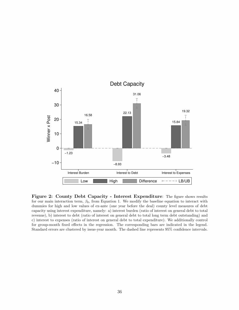
−1.23

−8.93

−3.48

15.34

22.13

15.84

16.58

31.06

19.32

−10

0

10

20

30

40

Win

ner

x P

ost

Interest Burden Interest to Debt Interest to Expenses

Low High Difference LB/UB

Debt Capacity

Figure 2: County Debt Capacity - Interest Expenditure: The figure shows resultsfor our main interaction term, β0, from Equation 1. We modify the baseline equation to interact withdummies for high and low values of ex-ante (one year before the deal) county level measures of debtcapacity using interest expenditure, namely: a) interest burden (ratio of interest on general debt to totalrevenue), b) interest to debt (ratio of interest on general debt to total long term debt outstanding) andc) interest to expenses (ratio of interest on general debt to total expenditure). We additionally controlfor group-month fixed effects in the regression. The corresponding bars are indicated in the legend.Standard errors are clustered by issue-year month. The dashed line represents 95% confidence intervals.

36

16.83

14.71

−2.48

−5.06

−0.880.37

19.31 19.77

−10

0

10

20

30

Win

ne

r x P

ost

Aggregating upto 3 years before deal Aggregating upto 5 years before deal

Low Medium High Difference LB/UB

Firm Value of Patents

(a)

7.01

1.71

3.12

5.30

0

2

4

6

8

10

Win

ne

r x P

ost

Low Medium High Difference LB/UB

Industry Level Jobs Multiplier

(b)

-2.71

-8.72

13.76

7.05 8.16

-6.90

-20

-10

0

10

20

Win

ner x

Pos

t

Manufa

cturin

g

Non-Trad

eable

s

Data C

entre

s

Wareho

using

Mining

All Othe

r

Industry of Deal

(c)

Figure 3: Expected Multiplier Effect: The figure shows results for our main interactionterm, β0, from Equation 1. We modify the baseline equation to interact with dummies corresponding tothe firm value of patents (sub-figure(a)), industry level jobs multiplier (sub-figure(b)) and the industryof the deal (sub-figure(c)). We additionally control for group-month fixed effects in the regression. Insub-figure (a), we show results by aggregating the value of patents at the firm level 3 years and 5 yearsbefore the deal, respectively. Jobs multipliers in sub-figure (b) are obtained from Economic PolicyInstitute. Industry groups in sub-figure (c) of the recipient firms are based on NAICS classification,which are recombined further. Specifically, non-tradeables include wholesale trade and retail trade.Data centers include professional and scientific, finance and insurance, information, and managementand administrative sectors. Mining is a combination of mining and energy, utilities, and construction.Warehousing includes transportation and warehousing, and real estate. Standard errors are clusteredby issue-year month. The dashed line represents 95% confidence intervals.

37

15.38

63.70

19.72

−0.04

4.80

0.11

−8.68

42.57

3.15

15.42

58.90

19.61

−20

0

20

40

60

80

Win

ner

x P

ost x H

igh

Interest Burden Interest to Debt Interest to Expenses

Firm Value of Patents

(a)

39.7441.66

44.24

−7.87 −7.47 −7.18

13.14

46.58

15.77

47.61 49.1251.42

−20

0

20

40

60

Win

ner

x P

ost x H

igh

Interest Burden Interest to Debt Interest to Expenses

Low Medium High Difference LB/UB

Industry Level Jobs Multiplier

(b)

Figure 4: Interaction of Debt Capacity with Multiplier Effect: The figure showsresults for the triple interaction term, β0, from Equation 5, interacted with the corresponding tercile ofmultiplier effect. Specifically, we modify the equation to interact with dummies corresponding to thesub-group of firm value of patents (sub-figure(a)) and industry level jobs multiplier (sub-figure(b)) atthe deal level. We additionally control for group-month fixed effects in the regression. In each figure,the triple interaction coefficient on the y-axis is shown with respect to the corresponding debt capacitymeasure. As before, we use interest burden, interest to debt and interest to expenses. A higher value ofinterest represents lower debt capacity. Standard errors are clustered by issue-year month. The dashedline represents 95% confidence intervals.

38

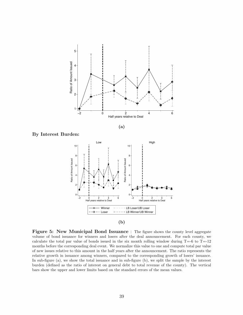
1

2

3

4

5

Ratio o

f A

mount Is

sued

−2 0 2 4 6Half years relative to Deal

(a)

By Interest Burden:

0

2

4

6

8

10

Ratio o

f A

mount Is

sued

−2 0 2 4 6Half years relative to Deal

Low

0

2

4

6

8

10

Ratio o

f A

mount Is

sued

−2 0 2 4 6Half years relative to Deal

High

Winner LB Loser/UB Loser

Loser LB Winner/UB Winner

(b)

Figure 5: New Municipal Bond Issuance : The figure shows the county level aggregatevolume of bond issuance for winners and losers after the deal announcement. For each county, wecalculate the total par value of bonds issued in the six month rolling window during T=-6 to T=-12months before the corresponding deal event. We normalize this value to one and compute total par valueof new issues relative to this amount in the half years after the announcement. The ratio represents therelative growth in issuance among winners, compared to the corresponding growth of losers’ issuance.In sub-figure (a), we show the total issuance and in sub-figure (b), we split the sample by the interestburden (defined as the ratio of interest on general debt to total revenue of the county). The verticalbars show the upper and lower limits based on the standard errors of the mean values.

39

By Interest Burden:

−100

0

100

200

300

Co

eff

icie

nt

−3 −2 −1 0 1 2 3Years relative to deal

Low

−100

0

100

200

300

Co

eff

icie

nt

−3 −2 −1 0 1 2 3Years relative to deal

High

(a) Property Tax Revenue per capita

−50

0

50

Co

eff

icie

nt

−3 −2 −1 0 1 2 3Years relative to deal

Low

−50

0

50

Co

eff

icie

nt

−3 −2 −1 0 1 2 3Years relative to deal

High

Winner LB/UB

Loser Difference

(b) FHFA House Price Index

Figure 6: Impact on Local Property Taxes: The figure represents the relative changes inproperty taxes among winners split by the interest burden, compared to the corresponding losers. Insub-figure (a), we show the property tax revenue and in sub-figure (b), we represent the house price indexobtained from Federal Housing Finance Agency ( FHFA). we use the annualized version of Equation 4,but additionally introduce county and event-year fixed effects. Here, we cluster standard errors at thedeal level. The benchmark period is the year before the window (-3,3). The dashed line represents 95%confidence intervals.

40

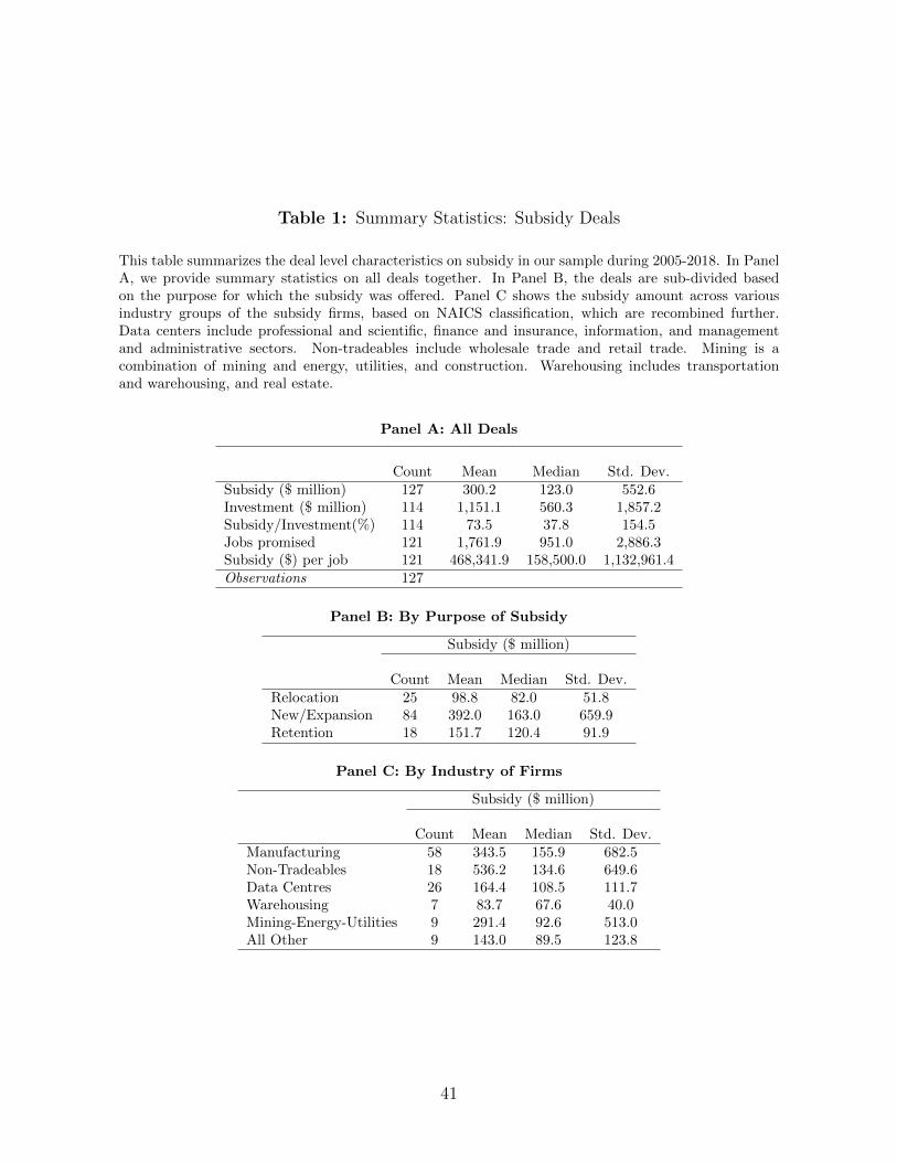
Table 1: Summary Statistics: Subsidy Deals

This table summarizes the deal level characteristics on subsidy in our sample during 2005-2018. In PanelA, we provide summary statistics on all deals together. In Panel B, the deals are sub-divided basedon the purpose for which the subsidy was offered. Panel C shows the subsidy amount across variousindustry groups of the subsidy firms, based on NAICS classification, which are recombined further.Data centers include professional and scientific, finance and insurance, information, and managementand administrative sectors. Non-tradeables include wholesale trade and retail trade. Mining is acombination of mining and energy, utilities, and construction. Warehousing includes transportationand warehousing, and real estate.

Panel A: All Deals

Count Mean Median Std. Dev.Subsidy ($ million) 127 300.2 123.0 552.6Investment ($ million) 114 1,151.1 560.3 1,857.2Subsidy/Investment(%) 114 73.5 37.8 154.5Jobs promised 121 1,761.9 951.0 2,886.3Subsidy ($) per job 121 468,341.9 158,500.0 1,132,961.4Observations 127

Panel B: By Purpose of Subsidy

Subsidy ($ million)

Count Mean Median Std. Dev.Relocation 25 98.8 82.0 51.8New/Expansion 84 392.0 163.0 659.9Retention 18 151.7 120.4 91.9

Panel C: By Industry of Firms

Subsidy ($ million)

Count Mean Median Std. Dev.Manufacturing 58 343.5 155.9 682.5Non-Tradeables 18 536.2 134.6 649.6Data Centres 26 164.4 108.5 111.7Warehousing 7 83.7 67.6 40.0Mining-Energy-Utilities 9 291.4 92.6 513.0All Other 9 143.0 89.5 123.8

41

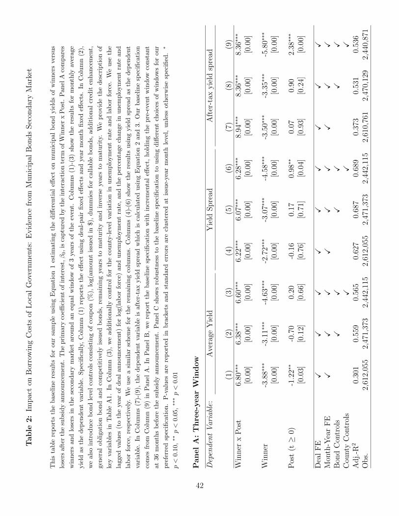
Table

2:

Impac

ton

Bor

row

ing

Cos

tsof

Loca

lG

over

nm

ents

:E

vid

ence

from

Munic

ipal

Bon

ds

Sec

ondar

yM

arke

t

Th

ista

ble

rep

orts

the

bas

elin

ere

sult

sfo

rou

rsa

mp

leu

sin

gE

qu

ati

on

1es

tim

ati

ng

the

diff

eren

tial

effec

ton

mu

nic

ipal

bon

dyie

lds

of

win

ner

sve

rsus

lose

rsaf

ter

the

sub

sid

yan

nou

nce

men

t.T

he

pri

mary

coeffi

cien

tof

inte

rest

,β0,

isca

ptu

red

by

the

inte

ract

ion

term

of

Win

ner

xP

ost

.P

an

elA

com

pare

s

win

ner

san

dlo

sers

inth

ese

con

dar

ym

arket

arou

nd

an

equ

al

win

dow

of

3ye

ars

of

the

even

t.C

olu

mn

s(1

)-(3

)sh

owth

ere

sult

sfo

rm

onth

lyav

erage

yie

ldas

the

dep

end

ent

vari

able

.S

pec

ifica

lly,

Col

um

n(1

)re

port

sth

eeff

ect

usi

ng

dea

l-p

air

fixed

effec

tsan

dye

ar

month

fixed

effec

ts.

InC

olu

mn

(2),

we

also

intr

od

uce

bon

dle

vel

contr

ols

con

sist

ing

of

cou

pon

(%),

log(a

mou

nt

issu

edin

$),

du

mm

ies

for

call

ab

leb

on

ds,

ad

dit

ion

al

cred

iten

han

cem

ent,

gen

eral

obli

gati

onb

ond

and

com

pet

itiv

ely

issu

edb

on

ds,

rem

ain

ing

years

tom

atu

rity

an

din

vers

eye

ars

tom

atu

rity

.W

ep

rovid

eth

ed

escr

ipti

on

of

key

vari

able

sin

Tab

leA

1.In

Col

um

n(3

),w

ead

dit

ion

all

yco

ntr

ol

for

the

cou

nty

-lev

elva

riati

on

inu

nem

plo

ym

ent

rate

an

dla

bor

forc

e.W

eu

seth

e

lagg

edva

lues

(to

the

year

ofd

eal

ann

oun

cem

ent)

for

log(l

ab

or

forc

e)an

du

nem

plo

ym

ent

rate

,an

dth

ep

erce

nta

ge

chan

ge

inu

nem

plo

ym

ent

rate

an

d

lab

orfo

rce,

resp

ecti

vely

.W

eu

sea

sim

ilar

schem

efo

rth

ere

main

ing

colu

mn

s.C

olu

mn

s(4

)-(6

)sh

owth

ere

sult

su

sin

gyie

ldsp

read

as

the

dep

end

ent

vari

able

.In

Col

um

ns

(7)-

(9),

the

dep

end

ent

vari

ab

leis

aft

er-t

ax

yie

ldsp

read

wh

ich

isca

lcu

late

du

sin

gE

qu

ati

on

2an

d3.

Ou

rb

ase

lin

esp

ecifi

cati

on

com

esfr

omC

olu

mn

(9)

inP

anel

A.

InP

anel

B,

we

rep

ort

the

base

lin

esp

ecifi

cati

on

wit

hin

crem

enta

leff

ect,

hold

ing

the

pre

-eve

nt

win

dow

con

stant

at36

mon

ths

bef

ore

the

sub

sid

yan

nou

nce

men

t.P

an

elC

show

sro

bu

stn

ess

toth

eb

ase

lin

esp

ecifi

cati

on

tou

sin

gd

iffer

ent

choic

esof

win

dow

sfo

rou

r

pre

ferr

edsp

ecifi

cati

on.

P-v

alu

esar

ere

por

ted

inb

rack

ets

an

dst

an

dard

erro

rsare

clu

ster

edat

issu

e-ye

ar

month

leve

l,un

less

oth

erw

ise

spec

ified

.∗

p<

0.10

,∗∗p<

0.0

5,∗∗∗p<

0.01

Pan

el

A:

Thre

e-y

ear

Win

dow

Depen

dentVariable:

Ave

rage

Yie

ldY

ield

Spre

adA

fter

-tax

yie

ldsp

read

(1)

(2)

(3)

(4)

(5)

(6)

(7)

(8)

(9)

Win

ner

xP

ost

6.80∗∗∗

6.38∗∗∗

6.60∗∗∗

6.22∗∗∗

6.07∗∗∗

6.28∗∗∗

8.94∗∗∗

8.36∗∗∗

8.36∗∗∗

[0.0

0][0

.00]

[0.0

0][0

.00]

[0.0

0][0

.00]

[0.0

0][0

.00]

[0.0

0]

Win

ner

-3.8

8∗∗∗

-3.1

1∗∗∗

-4.6

3∗∗∗

-2.7

2∗∗∗

-3.0

7∗∗∗

-4.5

8∗∗∗

-3.5

0∗∗∗

-3.3

5∗∗∗

-5.8

0∗∗∗

[0.0

0][0

.00]

[0.0

0][0

.00]

[0.0

0][0

.00]

[0.0

0][0

.00]

[0.0

0]

Pos

t(t

≥0)

-1.2

2∗∗

-0.7

00.

20-0

.16

0.17

0.98∗∗

0.07

0.90

2.38∗∗∗

[0.0

3][0

.12]

[0.6

6][0

.76]

[0.7

1][0

.04]

[0.9

3][0

.24]

[0.0

0]

Dea

lF

EX

XX

XX

XX

XX

Mon

th-Y

ear

FE

XX

XX

XX

XX

XB

ond

Con

trol

sX

XX

XX

XC

ounty

Con

trol

sX

XX

Adj.

-R2

0.30

10.

559

0.56

50.

627

0.68

70.

689

0.37

30.

531

0.53

6O

bs.

2,61

2,05

52,

471,

373

2,44

2,11

52,

612,

055

2,47

1,37

32,

442,

115

2,61

0,76

12,

470,

129

2,44

0,87

1

42

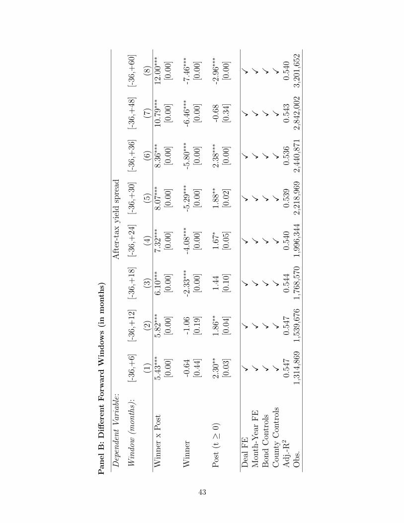
Pan

el

B:

Diff

ere

nt

Forw

ard

Win

dow

s(i

nm

onth

s)

DependentVariable:

Aft

er-t

axyie

ldsp

read

Window(m

onths)

:[-

36,+

6][-

36,+

12]

[-36

,+18

][-

36,+

24]

[-36

,+30

][-

36,+

36]

[-36

,+48

][-

36,+

60]

(1)

(2)

(3)

(4)

(5)

(6)

(7)

(8)

Win

ner

xP

ost

5.43∗∗∗

5.82∗∗∗

6.10∗∗∗

7.32∗∗∗

8.07∗∗∗

8.36∗∗∗

10.7

9∗∗∗

12.0

0∗∗∗

[0.0

0][0

.00]

[0.0

0][0

.00]

[0.0

0][0

.00]

[0.0

0][0

.00]

Win

ner

-0.6

4-1

.06

-2.3

3∗∗∗

-4.0

8∗∗∗

-5.2

9∗∗∗

-5.8

0∗∗∗

-6.4

6∗∗∗

-7.4

6∗∗∗

[0.4

4][0

.19]

[0.0

0][0

.00]

[0.0

0][0

.00]

[0.0

0][0

.00]

Pos

t(t

≥0)

2.30∗∗

1.86∗∗

1.44

1.67∗

1.88∗∗

2.38∗∗∗

-0.6

8-2

.96∗∗∗

[0.0

3][0

.04]

[0.1

0][0

.05]

[0.0

2][0

.00]

[0.3

4][0

.00]

Dea

lF

EX

XX

XX

XX

XM

onth

-Yea

rF

EX

XX

XX

XX

XB

ond

Con

trol

sX

XX

XX

XX

XC

ounty

Con

trol

sX

XX

XX

XX

XA

dj.

-R2

0.54

70.

547

0.54

40.

540

0.53

90.

536

0.54

30.

540

Ob

s.1,

314,

869

1,53

9,67

61,

768,

570

1,99

6,34

42,

218,

969

2,44

0,87

12,

842,

002

3,20

1,65

2

43

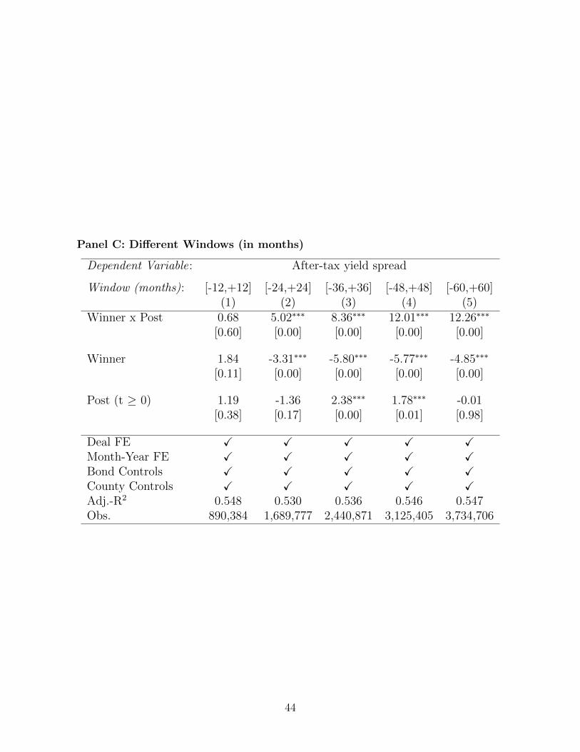
Panel C: Different Windows (in months)

Dependent Variable: After-tax yield spread

Window (months): [-12,+12] [-24,+24] [-36,+36] [-48,+48] [-60,+60](1) (2) (3) (4) (5)

Winner x Post 0.68 5.02∗∗∗ 8.36∗∗∗ 12.01∗∗∗ 12.26∗∗∗

[0.60] [0.00] [0.00] [0.00] [0.00]

Winner 1.84 -3.31∗∗∗ -5.80∗∗∗ -5.77∗∗∗ -4.85∗∗∗

[0.11] [0.00] [0.00] [0.00] [0.00]

Post (t ≥ 0) 1.19 -1.36 2.38∗∗∗ 1.78∗∗∗ -0.01[0.38] [0.17] [0.00] [0.01] [0.98]

Deal FE X X X X XMonth-Year FE X X X X XBond Controls X X X X XCounty Controls X X X X XAdj.-R2 0.548 0.530 0.536 0.546 0.547Obs. 890,384 1,689,777 2,440,871 3,125,405 3,734,706

44

Table 3: Robustness Tests

In this table we report results for various robustness test on our baseline specification, i.e., Column (9)

of Table 2. In Columns (1)-(3), we report results using only customer-buy trades with transaction size

≤ $25,000, ≤ $50,000 and ≤ $100,000, respectively. Columns (4)-(7) report regression results where

we drop bonds that are dated within 6 months, 12 months, 24 months and 36 months, respectively. In

Column (8), we use transactions after the financial crisis of 2009. Likewise, in Column (9), we show

results with deals after 2009. Column (10) shows the results with customer sell trades only. In Column

(11), we document the impact on state-level bonds for the bidding counties. We replace county-level

controls with lagged values of state revenue and state budget surplus. Columns (12)-(15) report results

with alternative choices of clustering the standard errors, namely: issuer-year month, issue-event

month, state-year month and deal-year month. In Column (16), we show the results for bonds with

non-missing S&P credit ratings. We use the most recent ratings for a given CUSIP. In Column (17), we

introduce additional county level time-varying covariates using lagged values of log(personal income)

and log(house price index). In Columns (18)-(20), we control for duration. First, in Column (18) we

use duration in the controls by replacing years to maturity and inverse of years to maturity. Second,

in Column (19), we use tax-adjusted duration to replace years to maturity and inverse of years to

maturity. Finally, Column (20) shows the result by using after-tax yield spread based on treasury

yields matched to duration (instead of remaining years to maturity) while simultaneously controlling

for duration instead of years to maturity and inverse of years to maturity. Columns (21)-(25) report

results controlling for unobserved factors at the county and state level. Specifically, in Column (21), we

introduce county fixed effect to the baseline. Column (22) shows results with county-year fixed effects

added to the baseline. In Column (23), we drop counties that may have overlapping bonds across deal

events. Any county which features in two or more deals as a bidder (winner or loser) over less than

6 years is dropped. Column (24) shows the results with state fixed effects added to the baseline. In

Column (25), we introduce state-year fixed effects. Columns (26)-(30) show the results with alternative

specifications. Specifically, Column (26) shows the results with bond fixed effects. We also require that

the bond should have at least one transaction before and after the deal announcement. The bond level

time-invariant controls get dropped. We also have to omit the years to maturity and inverse years

to maturity for consistent estimation of the variance co-variance matrix given our set of fixed effects.

Column (27) we introduce event-month fixed effects to the baseline. In Column (28), we drop the

year month fixed effects and replace it with the event-month fixed effects in the baseline. For Column

(29), we change the clustering of Column (28) from the baseline definition (of issue-year month) to

issue-event month. In Column (30), we show the results by replacing year-month fixed effects in the

baseline with year fixed effects. P-values are reported in brackets and standard errors are clustered at

issue-year month level, unless otherwise specified. ∗ p < 0.10, ∗∗ p < 0.05, ∗∗∗ p < 0.01

45

DependentVariable:

Aft

er-t

axyie

ldsp

read

Tra

nsa

ctio

nSiz

e($

)D

rop

Bon

ds

Dat

edW

ith

inF

inan

cial

Cri

sis

Oth

erT

rad

es

≤25

,000

≤50

,000

≤10

0,00

06

mon

ths

12m

onth

s24

mon

ths

36m

onth

sU

seT

rad

es>

2009

Use

Dea

ls>

2009

Sel

lT

rad

esS

tate

-lev

elB

ond

s(1

)(2

)(3

)(4

)(5

)(6

)(7

)(8

)(9

)(1

0)(1

1)

Win

ner

xP

ost

10.9

4∗∗∗

10.1

9∗∗∗

9.82∗∗∗

7.46∗∗∗

6.67∗∗∗

5.93∗∗∗

5.01∗∗∗

5.83∗∗∗

8.03∗∗∗

5.90∗∗∗

1.39∗∗∗

[0.0

0][0

.00]

[0.0

0][0

.00]

[0.0

0][0

.00]

[0.0

0][0

.00]

[0.0

0][0

.00]

[0.0

0]

Adj.

-R2

0.56

10.

559

0.55

70.

528

0.52

00.

501

0.48

00.

461

0.47

90.

511

0.57

9O

bs.

1,67

1,46

62,

006,

739

2,17

6,37

22,

286,

940

2,14

8,44

31,

860,

059

1,57

5,19

01,

690,

678

1,68

7,08

82,

173,

656

5,00

4,49

8

Clu

ster

ing

Addit

ional

Con

trol

sC

ontr

olling

for

Dura

tion

Issu

er-Y

MIs

sue-

Eve

nt

Mon

thSta

te-Y

MD

eal-

YM

Add

Rat

ings

Mor

eC

ounty

Con

trol

sU

seD

ura

tion

Use

afte

r-ta

xdura

tion

Dura

tion

adju

sted

spre

ad(1

2)(1

3)(1

4)(1

5)(1

6)(1

7)(1

8)(1

9)(2

0)

Win

ner

xP

ost

8.36∗∗∗

8.36∗∗∗

8.36∗∗∗

8.36∗∗∗

11.8

7∗∗∗

6.67∗∗∗

10.2

1∗∗∗

10.5

7∗∗∗

10.1

9∗∗∗

[0.0

0][0

.00]

[0.0

0][0

.00]

[0.0

0][0

.00]

[0.0

0][0

.00]

[0.0

0]

Adj.

-R2

0.53

60.

536

0.53

60.

536

0.58

90.

544

0.52

60.

499

0.75

8O

bs.

2,44

0,87

12,

440,

871

2,44

0,87

12,

440,

871

1,87

8,73

02,

190,

155

2,33

9,99

32,

339,

993

2,33

9,99

3

Un

obse

rvab

les:

Cou

nty

and

Sta

teO

ther

Sp

ecifi

cati

ons

Use

Use

Cou

nty

-D

rop

Cou

nti

esU

seU

seS

tate

-U

seA

dd

Eve

nt-

Rep

lace

YM

FE

toC

lust

erby

Issu

e-R

epla

cem

onth

FE

Cou

nty

FE

Yea

rF

Ew

ith

Ove

rlap

Sta

teF

EY

ear

FE

Bon

dF

EM

onth

FE

even

t-m

onth

FE

even

tm

onth

wit

hye

arF

E(2

1)(2

2)(2

3)(2

4)(2

5)(2

6)(2

7)(2

8)(2

9)(3

0)

Win

ner

xP

ost

10.5

4∗∗∗

2.87∗∗∗

13.4

2∗∗∗

11.4

8∗∗∗

3.16∗∗∗

3.95∗∗∗

8.35∗∗∗

9.31∗∗∗

9.31∗∗∗

11.2

5∗∗∗

[0.0

0][0

.00]

[0.0

0][0

.00]

[0.0

0][0

.00]

[0.0

0][0

.00]

[0.0

0][0

.00]

Ad

j.-R

20.

545

0.55

40.

584

0.54

20.

551

0.82

70.

536

0.35

30.

353

0.45

1O

bs.

2,44

0,87

12,

440,

860

936,

385

2,44

0,87

12,

440,

871

1,91

2,60

32,

440,

871

2,44

0,87

12,

440,

871

2,44

0,87

1

46

Table 4: County Debt Capacity: Evidence based on Credit Ratings

This table shows the evidence based on ex-ante county level ratings among winning counties, using

the baseline Equation 1. To control for the average impact within a particular group for that month

we add group-month fixed effects. We then interact the main equation with dummies corresponding

to the average S&P rating group of the county during -12 to -24 months before the deal. The rating

group belonging to AA- and above corresponds to higher credit rating quality, while A+ and below

represent lower credit quality. First, in Columns (1), we show the impact on the full sample of bonds for

which county level ratings are available in the benchmark period (-12 to -24 months) using all bonds.

Second, in Column (2), we replicate this approach using a sub-sample of general obligation (GO) bonds

only. Finally, Column (3) shows the impact on revenue (RV) bonds alone. P-values are reported in

brackets and standard errors are clustered at issue-year month level. ∗ p < 0.10, ∗∗ p < 0.05, ∗∗∗ p < 0.01

Dependent Variable: After-tax Yield Spread

All Bonds GO Bonds RV BondsWinner x Post (1) (2) (3)AA- and above 5.89∗∗∗ -6.74∗∗∗ 5.35∗∗

[0.00] [0.00] [0.01]

A+ and below 8.45∗∗∗ 16.69∗∗∗ 7.31∗∗∗

[0.00] [0.00] [0.00]Difference 2.552 23.43 1.955p-val 0.18 0.00 0.45Deal FE X X XMonth-Year FE X X XCounty Controls X X XGroup-Month FE X X XAdj.-R2 0.524 0.544 0.526Obs. 2,140,846 702,235 1,410,426

47

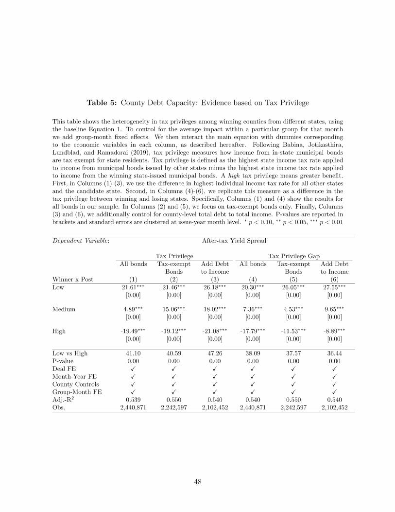
Table 5: County Debt Capacity: Evidence based on Tax Privilege

This table shows the heterogeneity in tax privileges among winning counties from different states, usingthe baseline Equation 1. To control for the average impact within a particular group for that monthwe add group-month fixed effects. We then interact the main equation with dummies correspondingto the economic variables in each column, as described hereafter. Following Babina, Jotikasthira,Lundblad, and Ramadorai (2019), tax privilege measures how income from in-state municipal bondsare tax exempt for state residents. Tax privilege is defined as the highest state income tax rate appliedto income from municipal bonds issued by other states minus the highest state income tax rate appliedto income from the winning state-issued municipal bonds. A high tax privilege means greater benefit.First, in Columns (1)-(3), we use the difference in highest individual income tax rate for all other statesand the candidate state. Second, in Columns (4)-(6), we replicate this measure as a difference in thetax privilege between winning and losing states. Specifically, Columns (1) and (4) show the results forall bonds in our sample. In Columns (2) and (5), we focus on tax-exempt bonds only. Finally, Columns(3) and (6), we additionally control for county-level total debt to total income. P-values are reported inbrackets and standard errors are clustered at issue-year month level. ∗ p < 0.10, ∗∗ p < 0.05, ∗∗∗ p < 0.01

Dependent Variable: After-tax Yield Spread

Tax Privilege Tax Privilege GapAll bonds Tax-exempt Add Debt All bonds Tax-exempt Add Debt

Bonds to Income Bonds to IncomeWinner x Post (1) (2) (3) (4) (5) (6)Low 21.61∗∗∗ 21.46∗∗∗ 26.18∗∗∗ 20.30∗∗∗ 26.05∗∗∗ 27.55∗∗∗

[0.00] [0.00] [0.00] [0.00] [0.00] [0.00]

Medium 4.89∗∗∗ 15.06∗∗∗ 18.02∗∗∗ 7.36∗∗∗ 4.53∗∗∗ 9.65∗∗∗

[0.00] [0.00] [0.00] [0.00] [0.00] [0.00]

High -19.49∗∗∗ -19.12∗∗∗ -21.08∗∗∗ -17.79∗∗∗ -11.53∗∗∗ -8.89∗∗∗

[0.00] [0.00] [0.00] [0.00] [0.00] [0.00]

Low vs High 41.10 40.59 47.26 38.09 37.57 36.44P-value 0.00 0.00 0.00 0.00 0.00 0.00Deal FE X X X X X XMonth-Year FE X X X X X XCounty Controls X X X X X XGroup-Month FE X X X X X XAdj.-R2 0.539 0.550 0.540 0.540 0.550 0.540Obs. 2,440,871 2,242,597 2,102,452 2,440,871 2,242,597 2,102,452

48

Table 6: Bargaining Power of Winning Counties

This table shows the heterogeneity in bargaining power across counties and states, using the baselineEquation 1. Group-month fixed effects are added in addition, to control for the average impact withina particular group for that month. We then interact the main equation with dummies corresponding

to the economic variables in each column, as described hereafter. Column (1) showsFirmAssets

CountyRevenuedenoting the ratio of the lagged value of firm assets to lagged county revenue of the winner. A highvalue of the ratio indicates low bargaining power of the county. In Column (2), we use the ratio ofsubsidy to lagged value of county-level budget surplus to create the three groups. Counties which had topay a large amount of subsidy in comparison to their budget surplus would represent higher desperationand lower bargaining power. Column (3) shows the interactions based on Intensity of Competition.We use the gap between winning and losing states in their budget surplus to revenue coverage ratiosas proxy for intensity of bidding competition. A low gap in ratios denotes high bidding competitionleading to low bargaining power for the winner. In Column (4) we provide evidence from the ex-anteUnemployment Rate of the winning counties in the year before the deal. P-values are reported inbrackets and standard errors are clustered at issue-year month level. ∗ p < 0.10, ∗∗ p < 0.05, ∗∗∗ p < 0.01

Dependent Variable: After-tax Yield Spread

Firm Assets Subsidy Intensity of UnemploymentCounty Revenue County Surplus Competition Rate

Winner x Post (1) (2) (3) (4)Low -4.50∗∗∗ -11.53∗∗∗ -5.73∗∗∗ -4.10∗∗∗

[0.00] [0.00] [0.00] [0.00]

Medium 5.73∗∗∗ 16.15∗∗∗ 10.76∗∗∗ -1.07[0.00] [0.00] [0.00] [0.51]

High 14.52∗∗∗ 19.37∗∗∗ 20.86∗∗∗ 22.32∗∗∗

[0.00] [0.00] [0.00] [0.00]

High vs Low 19.02 30.91 26.59 26.42P-value 0.00 0.00 0.00 0.00Deal FE X X X XMonth-Year FE X X X XCounty Controls X X X XGroup-Month FE X X X XAdj.-R2 0.543 0.537 0.538 0.537Obs. 2,030,786 2,427,378 2,438,182 2,438,182

49

Table 7: Impact on Primary Market of Municipal Bonds

This table shows the effect of subsidy announcement on new bond issuances using a difference-in-

differences estimate similar to the baseline specification. It is based on primary market bonds in

Equation 1, for offering yields. In Column (1), we show the result by using only the deal fixed effects

and issuer fixed effects in the baseline equation. Next, in Column (2), we introduce bond level controls.

Column (3) shows the results with county controls. Finally, Column (4) shows the results with rating

controls also added to the specification. We use S & P credit ratings at the time of issuance. P-values

are reported in brackets and standard errors are clustered at issue-dated month level. ∗ p < 0.10, ∗∗

p < 0.05, ∗∗∗ p < 0.01

Dependent Variable: Offering Yield

(1) (2) (3) (4)Winner x Post 11.61∗∗∗ 6.21∗∗∗ 4.59∗∗∗ 4.71∗∗∗

[0.00] [0.00] [0.00] [0.01]

Winner -5.56 -6.18∗∗ -0.42 -0.33[0.14] [0.04] [0.89] [0.92]

Post (t ≥ 0) -46.18∗∗∗ -36.93∗∗∗ -35.78∗∗∗ -36.59∗∗∗

[0.00] [0.00] [0.00] [0.00]

Deal FE X X X XIssuer FE X X X XBond Controls X X XCounty Controls X XRating Controls XAdj.-R2 0.421 0.824 0.833 0.835Obs. 343,519 340,241 336,559 217,414

50

For Online Publication–Internet Appendix

A Corporate Subsidies in the U.S.

Since colonial times, businesses have been offered tax-related incentives (Eisinger and La, 1988; Taylor,1993). Buss (2001) provides some interesting details about the history of subsidy competition. Even asearly as 1800, states financed infrastructure and offered capital to businesses. For example, Pennsylvaniahad invested USD 100 million in more than 150 corporations and placed directors on their boardsby 1844. While intense rivalry between Pittsburgh and Philadelphia led to substantial investmentin public infrastructure, widespread corruption also ensued. As a result, constitutional amendmentsoutlawed some of these practices (Watson, 1995). Relevant to many deals in our setting, Mississippipioneered tax-exempt municipal bonds to attract industries in 1936. Subsequently, by 1959, 21 stateshad established state-level business development corporations. Much of this new economic developmentwas often financed through debt. In the later part of the 20th century, the unemployment crises of the1970s and the recessions in early 1980s resulted in an aggressive war between states to win/retain jobs.

Chi and Leatherby (1997) document 15 most common business tax incentives ranging from corporateand personal tax exemption to various forms of tax credits related to job creation or research anddevelopment. Hanson (2019) provides some broad conclusions about the usefulness of different types oftax incentives. Property taxes and tax concessions are fully capitalized into property values. Whereas,tax increment financing (TIF) is not an effective economic redevelopment tool. On the other hand,increasing the corporate tax rate reduces employment and decreases business entry. Even so, there hasbeen justification for such tax incentives with various motivations: protecting (retaining) businesses frombeing lost to other states, shielding businesses from competition, revitalizing failing firms (Ambrosius,1989; Burnier, 1992; Wolman, 1988) or attracting new firms from outside. When most states offer suchsubsidy bids and incentives, other states also make room for such developmental tools (Gilbert, 1995).There is also an argument made in favor of subsidies since these are revenues forgone but not actualcash paid out. Another justification comes from Noll and Zimbalist (2011): if society has underemployedresources then that could be used more productively through corporate incentive programs. The primarydifficulty in understanding the overall impact of using subsidies for local economic development stemsfrom the endogeneity: policy changes/moves are directly correlated with outcomes of interest (Hanson,2019). In this regard, Hanson and Rohlin (2018) provides a detailed toolkit of methods and best practicesin evaluating spatially targeted urban redevelopment incentives. We try to incorporate some of thoserecommendations in our methodology and identification.

B Data on Corporate Subsidies in the U.S.

Subsidy Deals

The Good Jobs First Subsidy Tracker (Mattera, 2016) provides a starting point with its compilationon establishment-level spending data. They source these data from the state level dossiers on revenueforegone/credit offered in the Tax Expenditure Reports. Further, states also report incentives allocatedthrough various programs provided by their respective economic development offices. Such disclosuresare usually cited in the annual (or biennial) state-level budgets. The state Department of Revenue orBudget Office may be responsible for updating and maintaining such (web) archives. Still other statesthat do not report establishment-level monetary spending through subsidies in their financial data arealso present in the Subsidy Tracker dataset. News articles, press releases, and Freedom of InformationAct (FOIA) requests are used/cited in the dataset for these additional deals. However, the Good JobsFirst does not exhaustively contain all the subsidy programs launched and run by various states. Atbest, it may be most relevant for the larger set of discretionary subsidies floated by states and localgovernments. Overall, the existing dataset reports state-year level observations. For our purposes, thedataset needs to be enhanced with key variables that are not already recorded.

As of June 2018, the Subsidy Tracker files contained 606,899 records of subsidy items listed in theirfull dataset. We focus on records after 1990, wherein the year of subsidy is not missing. Also, our settingrequires bidding competition between non-federal governments. Hence, we omit deals where the moneyis sponsored by the federal government of United States. This further omits 221,000 records. (FigureIA1 brings out the proportion of federal versus non-federal incentives.) As a further check to verifyagainst federal money sponsoring some of these deals, we check the raw data included in our samplefor loans granted by the US government. While some of the composite subsidy packages may containcomponents offered by the US government, the total subsidy listed under state-level deals excludes thesefederal loans. In order to focus on large, economically meaningful deals for the local governments, werestrict our sample to subsidy values exceeding USD 50 million. After dropping such records, we areleft with 573 observations, which have to be manually parsed further because they include repetitionsat the firm or parent company level. Due to a lack of consistent nomenclature of firms, we parse thisinformation through careful reading. Specifically, a “Megadeal” may include various incentives stitched

1

together from money/tax abatement offered by the city, town, county and state governments. TheSubsidy Tracker data may or may not include overlapping items at the state level. For instance, in 2006the state of Florida offered USD 310 million as subsidy to Burnham Institute for Medical Research tolocate their medical research facility in Orlando (Orange County), which included USD 155.3 million fromthe Innovation Incentive Fund. Given the existing overlap in the raw Subsidy Tracker data, both theseobservations show up after the above filters. Florida statutes list an Innovation Incentive Program17 ‘torespond expeditiously to extraordinary economic opportunities and to compete effectively for high-valueresearch and development, innovation business, and alternative and renewal energy projects.’ In archivalreports, grants approved under the scheme date back to 1995–96.

Narrowing down to 2005–2018 for our sample period, we get 437 records. This imposition of calendaryears chosen is based on the availability of secondary market transactions in municipal bonds, describedlater. From the variables listed by Good Jobs First, we are primarily interested in the company name,parent firm, firm location, year, subsidy amount, subsidy adjusted, level of subsidy (based on the govern-ment level), city/county of the facility, number of jobs promised and total investment. There are cases ofmissing information. Additional data is gathered to plug in the FIPS code for the county, NAICS codefor the proposed facility or firm, and the purpose of the subsidy: new plant/expansion, retention, orrelocation. To distinguish between retention versus expansions, we rely on documented evidence in thenewspaper articles. A retention must be for a facility already operating in a location; whereas, expansionsmay be a new unit/assembly line. Understandably, retentions are often without any fresh investmentsmade by the firms. However, significant effort is devoted to comprehensively parse through local printmedia/newspapers to find out the losing county (and state) and earliest date of announcement for thesubsidy/plant. These two variables were the most painstaking aspects of the data collection procedure.In this context, our dataset construction is more granular and focused than Slattery (2018), who usesstate-level bidding competition. The Subsidy Tracker dataset never provides information on the losingcounty nor the precise announcement date. In Table IA1, we show a comparison of the original datasetversus the one constructed after hand-collection of relevant variables.

Through a careful manual reading of the newspaper articles, we can identify 127 winner-loser dealpairs at the county level, which we define as consisting our final sample18. Of these, 39 deal pairs overlapwith those used in Bloom, Brynjolfsson, Foster, Jarmin, Patnaik, Saporta-Eksten, and Van Reenen(2019). Where it was not possible to reasonably align a winning/losing city to a single county, allcounties were included. Since losing county information in these articles is worded very differently, itis challenging to automate the process through a programmed algorithm. We argue that given theincongruity between the size of the state and the subsidy offered, the local governments’ lens wouldbe more relevant as a setting, in terms of proportion. Motivated by reasons similar to those cited inBertrand and Mullainathan (2003) on using the exact dates of law passage for announcement effectsof anti-takeover provisions, we rely on earliest available dates for a given deal. Specifically, if date ofincentive approval/announcement is before the plant announcement date, we use this date because themarket already learns of the potential subsidy offer. However, occasionally, the facility announcementpredates the precise disclosures on all incentives that may have been offered to lure in the firm.

There is inherent secrecy maintained by local government and economic development board officialsabout such subsidy offers. The underlying assumption being that disclosures would invite other com-petitors; alternatively, invite moral hazard problems for counties that may be desperately keen to winnew jobs. For instance, consider the case of Burnham Institute for Medical Research in choosing Floridain 2006. Local officials refused to share details of the economic incentives bid in the public media for fearof instigating more competition from other locations/bidders (See Figure IA10). A snapshot of someproject names attributed to subsidy deals is provided in Table IA2 of the Appendix.

Caveats

Moreover, state economic development boards often revamp their (web) archives when the officer/Governorin charge loses power. This also becomes a hurdle in collecting information. As indicated before, wedo not claim to have collected the full universe of the subsidies offered to corporations. In fact, doingso may complicate the task of identifying the impact of corporate subsidies on the local governments,based on insignificant amounts waived off in abatement. Also, there is no way to ascertain what subsidybid was offered by the runner-up county/location. Only in some cases, the newspaper stories carry thecompeting bid offered. Largely, this remains unobserved in the current setting - and we acknowledgethis as a major limitation in the data. Especially so, in cases where more than one city is known to havecompeted. For deals with multiple losers, there is no direct way to ascertain as to which among thosewas the closest to getting the deal. We base our judgment on subjective assessment of grammatical hintsavailable in the article documenting the story. Therefore, this is not a robust way to identify the closestrunner-up location. To replicate the inter-state competition, wherever possible, priority is offered to alocation outside the winning state in assigning the runner-up county (for multiple runners-up).

17https://tinyurl.com/y2jze7ys18As such, there are 120 unique firm-year level subsidy deals among bidding states.

2

Table

IA1:

Com

par

ison

ofSubsi

dy

Dat

aset

s

Th

ista

ble

pro

vid

esa

snap

shot

com

par

ison

ofth

ein

form

ati

on

on

sub

sid

yd

eals

bet

wee

nth

eori

gin

al

data

from

Good

Job

sF

irst

Su

bsi

dy

Tra

cker

and

the

com

ple

ted

dat

aset

pre

par

edaf

ter

han

d-c

oll

ecti

on

.P

an

elA

show

sa

sam

ple

of

data

avail

ab

lefr

om

Good

Job

sF

irst

.P

an

elB

show

sth

ein

form

atio

nav

aila

ble

inou

rco

mple

ted

dat

aset

.??

?d

enote

sth

at

som

ein

form

ati

on

may

be

avail

ab

le,

wh

ile

bla

nks

rep

rese

nt

no

info

rmati

on

avail

ab

le.

PanelA:Good

JobsFirst

Win

ner

Lose

rC

om

pan

yY

ear

Date

Subsi

dy

($m

il)

Inves

tmen

t($

mil)

Sta

teC

ounty

Sta

teC

ounty

Jobs

Purp

ose

Baxte

rIn

tern

atio

nal

2012

211

???

GA

???

???

???

Fox

conn

2017

479

21000

0W

IR

aci

ne

13000

???

Ver

tex

Pharm

aceu

tica

ls201

172

???

MA

???

500

???

PanelB:Completed

Data

set

Win

ner

Lose

rC

om

pan

yY

ear

Date

Subsi

dy

($m

il)

Inves

tmen

t($

mil)

Sta

teC

ounty

Sta

teC

ounty

Jobs

Purp

ose

Baxte

rIn

tern

atio

nal

2012

4/19/

2012

211

1000

GA

New

ton

NC

Durh

am

1500

New

Fox

conn

2017

7/26/2017

4792

100

00

WI

Raci

ne

MI

Way

ne

13000

New

Ver

tex

Pharm

aceu

tica

ls201

19/1

5/2011

72

2500

MA

Suff

olk

MA

Mid

dle

sex

500

Rel

oca

tion

3

Table IA2: Names of Projects (Amounts in $ million)

This table shows some examples of project names under which the respective bidding processes wereencoded by the winning local governments in order to maintain secrecy.

Company Year State Project Name Investment SubsidyEastman Chemical 2007 TN Reinvest 1,300 100Burnham Institute for Medical Research 2006 FL Power 90 310Freightquote 2012 MO Apple 44 64Airbus (EADS) 2012 AL Hope 600 158.5Northrop Grunman 2014 FL Magellan 500 471Benteler Steel/Tube 2012 LA Delta 900 81.75

Table IA3: Determinants of Subsidy

This table reports a linear regression of the amount of subsidy in our sample of deals for 2005-2018 onmetrics potentially linked to the incentive. P-values are reported in brackets and standard errors arerobust to heteroskedasticity. ∗ p < 0.10, ∗∗ p < 0.05, ∗∗∗ p < 0.01

Subsidy (USD million)

Jobs (1000) 136.58*** 95.22*** 93.88*** 111.42*** 68.25*** 64.92***[0.00] [0.00] [0.00] [0.00] [0.00] [0.00]

Investment (USD mil) 0.12** 0.12** 0.10*** 0.10*** 0.10***[0.04] [0.03] [0.00] [0.00] [0.00]

State Expenditure (USD mil) -0.25 -12.55[0.80] [0.17]

Median HH-Incomet−1(1000) -2.77 -3.09*[0.14] [0.07]

State Surplus Gap (USD mil) -3.81*[0.08]

Constant 52.61 -1.37 9.06 628.83 181.16* 200.18**[0.25] [0.98] [0.90] [0.15] [0.06] [0.03]

State FE X X XEvent-Year FE X X XAdj.-R2 0.507 0.617 0.613 0.761 0.825 0.832Obs. 121 112 111 104 96 96

4

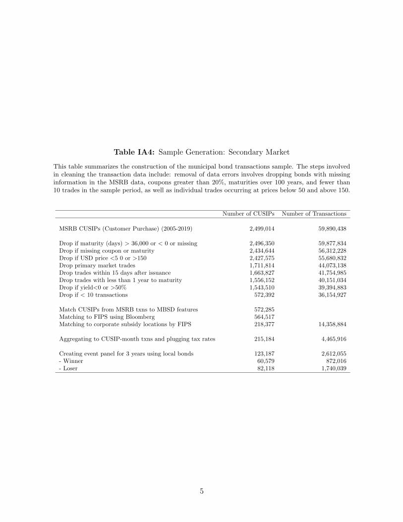
Table IA4: Sample Generation: Secondary Market

This table summarizes the construction of the municipal bond transactions sample. The steps involvedin cleaning the transaction data include: removal of data errors involves dropping bonds with missinginformation in the MSRB data, coupons greater than 20%, maturities over 100 years, and fewer than10 trades in the sample period, as well as individual trades occurring at prices below 50 and above 150.

Number of CUSIPs Number of Transactions

MSRB CUSIPs (Customer Purchase) (2005-2019) 2,499,014 59,890,438

Drop if maturity (days) > 36,000 or < 0 or missing 2,496,350 59,877,834Drop if missing coupon or maturity 2,434,644 56,312,228Drop if USD price <5 0 or >150 2,427,575 55,680,832Drop primary market trades 1,711,814 44,073,138Drop trades within 15 days after issuance 1,663,827 41,754,985Drop trades with less than 1 year to maturity 1,556,152 40,151,034Drop if yield<0 or >50% 1,543,510 39,394,883Drop if < 10 transactions 572,392 36,154,927

Match CUSIPs from MSRB txns to MBSD features 572,285Matching to FIPS using Bloomberg 564,517Matching to corporate subsidy locations by FIPS 218,377 14,358,884

Aggregating to CUSIP-month txns and plugging tax rates 215,184 4,465,916

Creating event panel for 3 years using local bonds 123,187 2,612,055- Winner 60,579 872,016- Loser 82,118 1,740,039

5

Table IA5: Summary Statistics: Municipal Bonds

This table summarizes the bond level characteristics for our sample of bonds linked to corporatesubsidies during 2005-2018. Panel A reports the secondary market attributes. Panel B reports theprimary market features. The key variables are described in Table A1.

Panel A: Secondary market

Count Mean Median Std. Dev.WinnerAverage Yield(%) 872,016 2.8 2.9 1.5Yield Spread(%) 872,016 1.4 1.2 1.8After-tax Yield Spread (%) 870,722 3.2 2.6 2.4Remaining Maturity (years) 872,016 10.0 8.8 7.1LoserAverage Yield(%) 1,740,039 2.7 2.8 1.5Yield Spread(%) 1,740,039 1.3 1.2 1.8After-tax Yield Spread (%) 1,740,039 3.2 2.6 2.4Remaining Maturity (years) 1,740,039 10.8 9.3 7.6Observations 2,612,055

Panel B: Primary market

Count Mean Median Std. Dev.WinnerOffering Yield(%) 134,475 2.8 2.9 1.4Offering Price ($) 134,499 103.7 101.7 7.4Coupon(%) 137,374 3.6 4.0 1.3Years to Maturity 137,374 9.3 8.2 6.5Years to Call 55,316 9.0 9.7 1.7Amount ($ million) 135,465 3.1 0.7 16.6Issue Size ($ million) 137,374 43.3 11.5 122.8LoserOffering Yield(%) 214,434 3.0 3.0 1.4Offering Price ($) 214,462 103.6 101.8 9.4Coupon(%) 218,222 3.7 4.0 1.3Years to Maturity 218,222 10.0 8.9 6.8Years to Call 95,862 8.8 9.7 2.1Amount ($ million) 214,503 5.0 0.8 22.6Issue Size ($ million) 218,222 84.1 14.3 196.0Observations 355,596

6

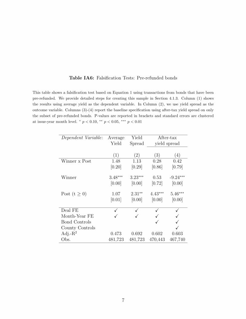
Table IA6: Falsification Tests: Pre-refunded bonds

This table shows a falsification test based on Equation 1 using transactions from bonds that have been

pre-refunded. We provide detailed steps for creating this sample in Section 4.1.3. Column (1) shows

the results using average yield as the dependent variable. In Column (2), we use yield spread as the

outcome variable. Columns (3)-(4) report the baseline specification using after-tax yield spread on only

the subset of pre-refunded bonds. P-values are reported in brackets and standard errors are clustered

at issue-year month level. ∗ p < 0.10, ∗∗ p < 0.05, ∗∗∗ p < 0.01

Dependent Variable: Average Yield After-taxYield Spread yield spread

(1) (2) (3) (4)Winner x Post 1.48 1.13 0.28 0.42

[0.20] [0.29] [0.86] [0.79]

Winner 3.48∗∗∗ 3.23∗∗∗ 0.53 -9.24∗∗∗

[0.00] [0.00] [0.72] [0.00]

Post (t ≥ 0) 1.07 2.31∗∗ 4.43∗∗∗ 5.46∗∗∗

[0.01] [0.00] [0.00] [0.00]

Deal FE X X X XMonth-Year FE X X X XBond Controls X XCounty Controls XAdj.-R2 0.473 0.692 0.602 0.603Obs. 481,723 481,723 470,443 467,740

7

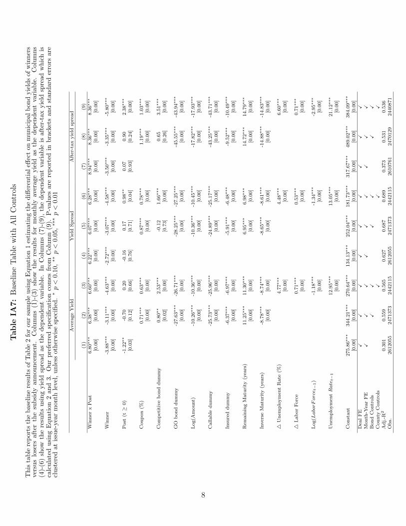
Table

IA7:

Bas

elin

eT

able

wit

hA

llC

ontr

ols

Th

ista

ble

rep

orts

the

bas

elin

ere

sult

sof

Tab

le2

for

ou

rsa

mp

leu

sin

gE

qu

ati

on

1es

tim

ati

ng

the

diff

eren

tial

effec

ton

mu

nic

ipal

bon

dyie

lds

of

win

ner

sve

rsu

slo

sers

afte

rth

esu

bsi

dy

ann

oun

cem

ent.

Colu

mn

s(1

)-(3

)sh

owth

ere

sult

sfo

rm

onth

lyav

erage

yie

ldas

the

dep

end

ent

vari

ab

le.

Colu

mn

s(4

)-(6

)sh

owth

ere

sult

su

sin

gyie

ldsp

read

asth

ed

epen

den

tva

riab

le.

InC

olu

mn

s(7

)-(9

),th

ed

epen

den

tva

riab

leis

aft

er-t

ax

yie

ldsp

read

wh

ich

isca

lcu

late

du

sin

gE

qu

atio

n2

and

3.O

ur

pre

ferr

edsp

ecifi

cati

on

com

esfr

om

Colu

mn

(9).

P-v

alu

esare

rep

ort

edin

bra

cket

san

dst

an

dard

erro

rsare

clu

ster

edat

issu

e-ye

arm

onth

leve

l,u

nle

ssot

her

wis

esp

ecifi

ed.∗p<

0.1

0,∗∗p<

0.05,∗∗∗p<

0.01

AverageYield

Yield

Spread

After-taxyield

spread

(1)

(2)

(3)

(4)

(5)

(6)

(7)

(8)

(9)

Winner

xPost

6.80∗∗

∗6.38∗∗

∗6.60∗∗

∗6.22∗∗

∗6.07∗∗

∗6.28∗∗

∗8.94∗∗

∗8.36∗∗

∗8.36∗∗

∗

[0.00]

[0.00]

[0.00]

[0.00]

[0.00]

[0.00]

[0.00]

[0.00]

[0.00]

Winner

-3.88∗∗

∗-3.11∗∗

∗-4.63∗∗

∗-2.72∗∗

∗-3.07∗∗

∗-4.58∗∗

∗-3.50∗∗

∗-3.35∗∗

∗-5.80∗∗

∗

[0.00]

[0.00]

[0.00]

[0.00]

[0.00]

[0.00]

[0.00]

[0.00]

[0.00]

Post

(t≥

0)

-1.22∗∗

-0.70

0.20

-0.16

0.17

0.98∗∗

0.07

0.90

2.38∗∗

∗

[0.03]

[0.12]

[0.66]

[0.76]

[0.71]

[0.04]

[0.93]

[0.24]

[0.00]

Coupon(%

)0.71∗∗

∗0.63∗∗

∗0.87∗∗

∗0.78∗∗

∗1.19∗∗

∗1.03∗∗

∗

[0.00]

[0.00]

[0.00]

[0.00]

[0.00]

[0.00]

Competitivebonddummy

0.80∗∗

2.53∗∗

∗-0.12

1.66∗∗

∗0.65

3.51∗∗

∗

[0.02]

[0.00]

[0.73]

[0.00]

[0.26]

[0.00]

GO

bonddummy

-27.63∗∗

∗-26.71∗∗

∗-28.25∗∗

∗-27.25∗∗

∗-45.55∗∗

∗-43.94∗∗

∗

[0.00]

[0.00]

[0.00]

[0.00]

[0.00]

[0.00]

Log(A

mount)

-10.26∗∗

∗-10.36∗∗

∗-10.36∗∗

∗-10.45∗∗

∗-17.82∗∗

∗-17.93∗∗

∗

[0.00]

[0.00]

[0.00]

[0.00]

[0.00]

[0.00]

Callable

dummy

-25.73∗∗

∗-25.96∗∗

∗-24.89∗∗

∗-25.17∗∗

∗-43.25∗∗

∗-43.71∗∗

∗

[0.00]

[0.00]

[0.00]

[0.00]

[0.00]

[0.00]

Insu

reddummy

-6.37∗∗

∗-6.97∗∗

∗-5.91∗∗

∗-6.48∗∗

∗-9.52∗∗

∗-10.49∗∗

∗

[0.00]

[0.00]

[0.00]

[0.00]

[0.00]

[0.00]

Rem

ainingMatu

rity

(yea

rs)

11.25∗∗

∗11.30∗∗

∗6.95∗∗

∗6.98∗∗

∗14.72∗∗

∗14.79∗∗

∗

[0.00]

[0.00]

[0.00]

[0.00]

[0.00]

[0.00]

Inverse

Matu

rity

(yea

rs)

-8.78∗∗

∗-8.74∗∗

∗-8.65∗∗

∗-8.61∗∗

∗-14.88∗∗

∗-14.83∗∗

∗

[0.00]

[0.00]

[0.00]

[0.00]

[0.00]

[0.00]

4Unem

ploymen

tRate

(%)

4.77∗∗

∗4.48∗∗

∗6.60∗∗

∗

[0.00]

[0.00]

[0.00]

4LaborForce

0.71∗∗

∗0.53∗∗

∗0.71∗∗

∗

[0.00]

[0.00]

[0.00]

Log(L

aborForce

t−1)

-1.18∗∗

∗-1.34∗∗

∗-2.95∗∗

∗

[0.00]

[0.00]

[0.00]

Unem

ploymen

tRate

t−1

12.95∗∗

∗13.05∗∗

∗21.12∗∗

∗

[0.00]

[0.00]

[0.00]

Constant

275.86∗∗

∗344.21∗∗

∗270.64∗∗

∗134.13∗∗

∗252.04∗∗

∗181.73∗∗

∗317.67∗∗

∗489.02∗∗

∗384.09∗∗

∗

[0.00]

[0.00]

[0.00]

[0.00]

[0.00]

[0.00]

[0.00]

[0.00]

[0.00]

Dea

lFE

XX

XX

XX

XX

XMonth

-Yea

rFE

XX

XX

XX

XX

XBondControls

XX

XX

XX

County

Controls

XX

XAdj.-R

20.301

0.559

0.565

0.627

0.687

0.689

0.373

0.531

0.536

Obs.

2612055

2471373

2442115

2612055

2471373

2442115

2610761

2470129

2440871

8

Table IA8: Trading Volume

This table reports the baseline results similar to Table 2 for our sample using Equation 1, with trading

volume as the dependent variable. Columns (1)-(2) show the results for a sub-sample of customer buy

trades. Columns (3)-(4) show the results for a sub-sample of customer sell trades. Finally, Columns

(5)-(6), use the sum total of buy and sell trades (wherever available) as the dependent variable in the

trading volume. P-values are reported in brackets and standard errors are clustered at issue-year month

level, unless otherwise specified. ∗ p < 0.10, ∗∗ p < 0.05, ∗∗∗ p < 0.01

Dependent Variable: Trading volume (bond-month)

Customer Buy Customer Sell Total(1) (2) (3) (4) (5) (6)

Winner x Post 36,860.38∗∗∗ 38,538.15∗∗∗ 44,894.96∗∗∗ 47,995.37∗∗∗ 87,101.09∗∗∗ 92,656.04∗∗∗

[0.00] [0.00] [0.00] [0.00] [0.00] [0.00]

Winner -22,669.41∗∗∗ -19,363.06∗∗∗ -24,175.89∗∗∗ -25,659.89∗∗∗ -45,544.56∗∗∗ -48,348.35∗∗∗

[0.00] [0.00] [0.00] [0.00] [0.00] [0.00]

Post (t ≥ 0) -24,621.30∗∗∗ -24,900.02∗∗∗ -11,735.60 -11,983.65 -33,091.52 -33,498.17[0.01] [0.01] [0.31] [0.30] [0.12] [0.12]

Deal FE X X X X X XMonth-Year FE X X X X X XBond Controls X X X X X XCounty Controls X X XAdj.-R2 0.049 0.049 0.047 0.047 0.053 0.053Obs. 2,471,373 2,442,115 1,971,026 1,951,056 1,971,026 1,951,056

9

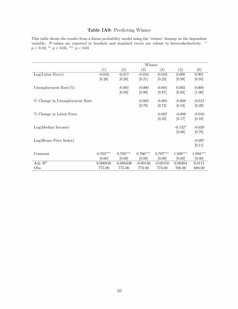
Table IA9: Predicting Winner

This table shows the results from a linear probability model using the ’winner’ dummy as the dependentvariable. P-values are reported in brackets and standard errors are robust to heteroskedasticity. ∗

p < 0.10, ∗∗ p < 0.05, ∗∗∗ p < 0.01

Winner(1) (2) (3) (4) (5) (6)

Log(Labor Force) -0.016 -0.017 -0.016 -0.016 0.000 0.001[0.20] [0.20] [0.21] [0.23] [0.98] [0.95]

Unemployment Rate(%) -0.001 -0.000 -0.001 0.002 0.000[0.93] [0.99] [0.87] [0.82] [1.00]

% Change in Unemployment Rate -0.005 -0.005 -0.008 -0.012[0.70] [0.72] [0.53] [0.39]

% Change in Labor Force -0.007 -0.009 -0.010[0.32] [0.17] [0.16]

Log(Median Income) -0.132∗ -0.028[0.06] [0.76]

Log(House Price Index) -0.097[0.11]

Constant 0.703∗∗∗ 0.709∗∗∗ 0.706∗∗∗ 0.707∗∗∗ 1.929∗∗∗ 1.988∗∗∗

[0.00] [0.00] [0.00] [0.00] [0.00] [0.00]Adj.-R2 0.000848 -0.000436 -0.00146 -0.00150 0.00384 0.0111Obs. 775.00 775.00 773.00 773.00 706.00 680.00

10

Table

IA10:

Impac

ton

Public

Exp

endit

ure

Th

ista

ble

show

sth

eim

pac

tof

sub

sid

yon

loca

lgov

ern

men

tex

pen

dit

ure

ssc

ali

ng

each

met

ric

at

the

per

cap

ita

level

.W

eu

seth

ean

nuali

zed

ver

sion

ofE

qu

atio

n1

asth

ep

rim

ary

spec

ifica

tion

for

this

tab

le.

Colu

mn

s(1

)-(4

)sh

owth

eaggre

gate

imp

act

per

cap

ita,

wh

ile

Colu

mn

s(5

)-(8

)p

rese

nt

the

resu

lts

bas

edon

sub

grou

ps

ofth

ein

tere

stb

urd

en.

Sp

ecifi

call

y,w

esh

owth

ein

tera

cted

form

of

the

diff

eren

ce-i

n-d

iffer

ence

ses

tim

ate

base

don

ad

um

my

vari

able

(Low

and

Hig

h)

bas

edon

the

med

ian

valu

eam

on

gw

inn

ing

cou

nti

es.

Inth

ese

inte

ract

edsp

ecifi

cati

on

s,w

ere

pla

ceth

eev

ent-

year

fixed

effec

tsw

ith

grou

p-e

vent

year

fixed

effec

tsto

ab

sorb

the

un

der

lyin

ggro

up

spec

ific

yea

rly

vari

ati

on

.P

-valu

esare

rep

ort

edin

bra

cket

san

dst

and

ard

erro

rsar

ecl

ust

ered

atth

ed

eal

leve

l.∗p<

0.1

0,∗∗p<

0.05,∗∗∗p<

0.01

Dep

enden

tV

ari

abl

e:

Tot

alE

lem

enta

ryH

ealt

hP

oli

cean

dT

otal

Ele

men

tary

Hea

lth

Poli

cean

dE

xp

end

itu

reE

du

cati

onP

rote

ctio

nE

du

cati

on

Pro

tect

ion

By

Inte

rest

Bu

rden

(1)

(2)

(3)

(4)

(5)

(6)

(7)

(8)

Win

ner

xP

ost

-24.

593.

80

-38.

58

-1.8

5[0

.63]

[0.8

6]

[0.2

5][0

.74]

Win

ner

xP

ost

x-1

4.09

-10.

056.6

00.4

9L

ow[0

.84]

[0.7

6][0

.91]

[0.9

5]

Win

ner

xP

ost

x-4

2.27

17.

77

-91.1

1∗∗∗

-5.3

6H

igh

[0.5

6][0

.54]

[0.0

0]

[0.5

1]

Low

vs

Hig

h28.

18-2

7.81

97.7

15.

844

P-v

alu

e0.7

80.5

30.

14

0.61

Dea

lF

EX

XX

XX

XX

XC

ounty

FE

XX

XX

XX

XX

Eve

nt-

Yea

rF

EX

XX

XG

rou

pE

vent-

Yea

rF

EX

XX

XC

ounty

Con

trol

sX

XX

XX

XX

XA

dj.

-R2

0.97

10.

956

0.982

0.9

73

0.97

10.9

56

0.9

820.9

72O

bs.

1,62

91,

629

1,62

91,6

291,

618

1,6

181,6

18

1,618

11

010

20

30

Am

ount in

US

D b

illion

2005

2006

2007

2008

2009

2010

2011

2012

2013

2014

2015

2016

2017

2018*

Non Federal Federal

Figure IA1: Total Subsidy: The vertical bars show the aggregated value of total subsidy offeredby federal and non-federal (state and local bodies) governments for each year during 2005-2018. Thisdoes not include federal loans. Calculated based on Source: Good Jobs First, Subsidy Tracker. *Denotesincomplete data for the year, till June 2018

010

20

30

Am

ount in

US

D b

illion

NY

LA

MI

WA

NJ

IN

OR

WI

TX

KY

MO

NC

TN

CT

IL

CA

AL

OH

NV

IA

MS

FL

PA

SC

MD

OK

GA

MN

MA

UT

NM

VA

CO

AR

KS

ME

AZ

RI

ID

WV

DE

NE

AK

VT

MT

NH

SD

ND

WY

HI

Figure IA2: Total Subsidy by States: The figure shows ranking among US states basedon total non-federal subsidy offered during 2005-2018. Calculated based on Source: Good Jobs First,Subsidy Tracker

12

Above 1,5001,000 − 1,500500 − 1,000200 − 500Below 200

Figure IA3: Subsidy per Capita: The state-level distribution of subsidy per capita (in USD)is shown for the period 2005-2018. Calculated based on Source: Good Jobs First, Subsidy Tracker

010

20

30

Fre

quency

50−75 75−100 100−200 200−500 >500

Figure IA4: Distribution of Subsidy (USD million): In this figure, we plot the numberof deals in our sample of winner-loser pairs during 2005-2018 across different ranges of subsidy bins.

13

−.02

0

.02

.04

.06

.08

Coeffic

ient

−3 −2 −1 0 1 2 3Years relative to deal

Winner Loser

LB/UB LB/UB

Log(Aggregate Employment)

(a)

−1

−.5

0

.5

1

Coeffic

ient

−3 −2 −1 0 1 2 3Years relative to deal

Winner Loser

LB/UB LB/UB

Unemployment Rate

(b)

−.6

−.4

−.2

0

.2

Coeffic

ient

−3 −2 −1 0 1 2 3Years relative to deal

Winner Loser

LB/UB LB/UB

Rating

(c)

−.02

−.01

0

.01

.02

Coeffic

ient

−3 −2 −1 0 1 2 3

Years relative to deal

Winner Loser

LB/UB LB/UB

Local Beta

(d)

Figure IA5: Identifying Assumption - Local Economy: The figure shows the localeconomic conditions at the county level between the bidding counties, around the event of subsidyannouncement. we use the annualized version of Equation 4, but additionally introduce county fixedeffects. Here, we cluster standard errors at the deal level. The benchmark period is the year before thewindow (-3,3). The dashed line represents 95% confidence intervals.

14

Log(Labor Force)

Unemployment Rate(%)

% Change in Unemployment Rate

% Change in Labor Force

Log(Median Income)

Log(House Price Index)

−.2 −.1 0 .1 .2

Figure IA6: Predicting Winners: This figure reports the regression coefficients of a linearprobability model predicting the winners using local economic variables. We use local economic variables3 years before the deal. Confidence intervals at the 95% level are plotted.

15

5.117.06

−5.24

21.19

−8.33

−10

0

10

20

30

Win

ne

r x P

ost

Primar

y Edu

catio

n

Dev

elop

men

t

Oth

er P

ublic

Ser

vice

s

Infra

stru

ctur

e

Wat

er−S

ewer

Purpose of Bond

(a)

0.77

7.11

12.44

0

5

10

15

Win

ne

r x P

ost

0 to

5 yea

rs

5 to

10

year

s

Ove

r 10

year

s

Duration

(b)

Figure IA7: Use of Proceeds: The figure shows results for our main interaction term, β0,from Equation 1. We modify the baseline equation to interact with dummies corresponding to the useof proceeds (sub-figure(a)) and duration (sub-figure(b)). We additionally control for group-month fixedeffects in the regression. The classification of purpose of bond is based on use of proceeds similar toGao, Lee, and Murphy (2019b)

16

By Interest to Debt:

−100

0

100

200

300

Co

eff

icie

nt

−3 −2 −1 0 1 2 3Years relative to deal

Low

−100

0

100

200

300

Co

eff

icie

nt

−3 −2 −1 0 1 2 3Years relative to deal

High

(a) Property Tax Revenue per capita

−100

−50

0

50

Co

eff

icie

nt

−3 −2 −1 0 1 2 3Years relative to deal

Low

−100

−50

0

50

Co

eff

icie

nt

−3 −2 −1 0 1 2 3Years relative to deal

High

Winner LB/UB

Loser Difference

(b) FHFA House Price Index

Figure IA8: Impact on Local Property Taxes: The figure represents the relative changesin property taxes among winners split by the interest to debt, compared to the corresponding losers. Insub-figure (a), we show the property tax revenue and in sub-figure (b), we represent the house price indexobtained from Federal Housing Finance Agency ( FHFA). we use the annualized version of Equation 4,but additionally introduce county and event-year fixed effects. Here, we cluster standard errors at thedeal level. The benchmark period is the year before the window (-3,3). The dashed line represents 95%confidence intervals.

17

By Interest to Expenses:

−100

0

100

200

300

Co

eff

icie

nt

−3 −2 −1 0 1 2 3Years relative to deal

Low

−100

0

100

200

300

Co

eff

icie

nt

−3 −2 −1 0 1 2 3Years relative to deal

High

(a) Property Tax Revenue per capita

−50

0

50

Co

eff

icie

nt

−3 −2 −1 0 1 2 3Years relative to deal

Low

−50

0

50

Co

eff

icie

nt

−3 −2 −1 0 1 2 3Years relative to deal

High

Winner LB/UB

Loser Difference

(b) FHFA House Price Index

Figure IA9: Impact on Local Property Taxes: The figure represents the relative changesin property taxes among winners split by the interest to expenses, compared to the corresponding losers.In sub-figure (a), we show the property tax revenue and in sub-figure (b), we represent the house priceindex obtained from Federal Housing Finance Agency ( FHFA). we use the annualized version of Equation4, but additionally introduce county and event-year fixed effects. Here, we cluster standard errors at thedeal level. The benchmark period is the year before the window (-3,3). The dashed line represents 95%confidence intervals.

18

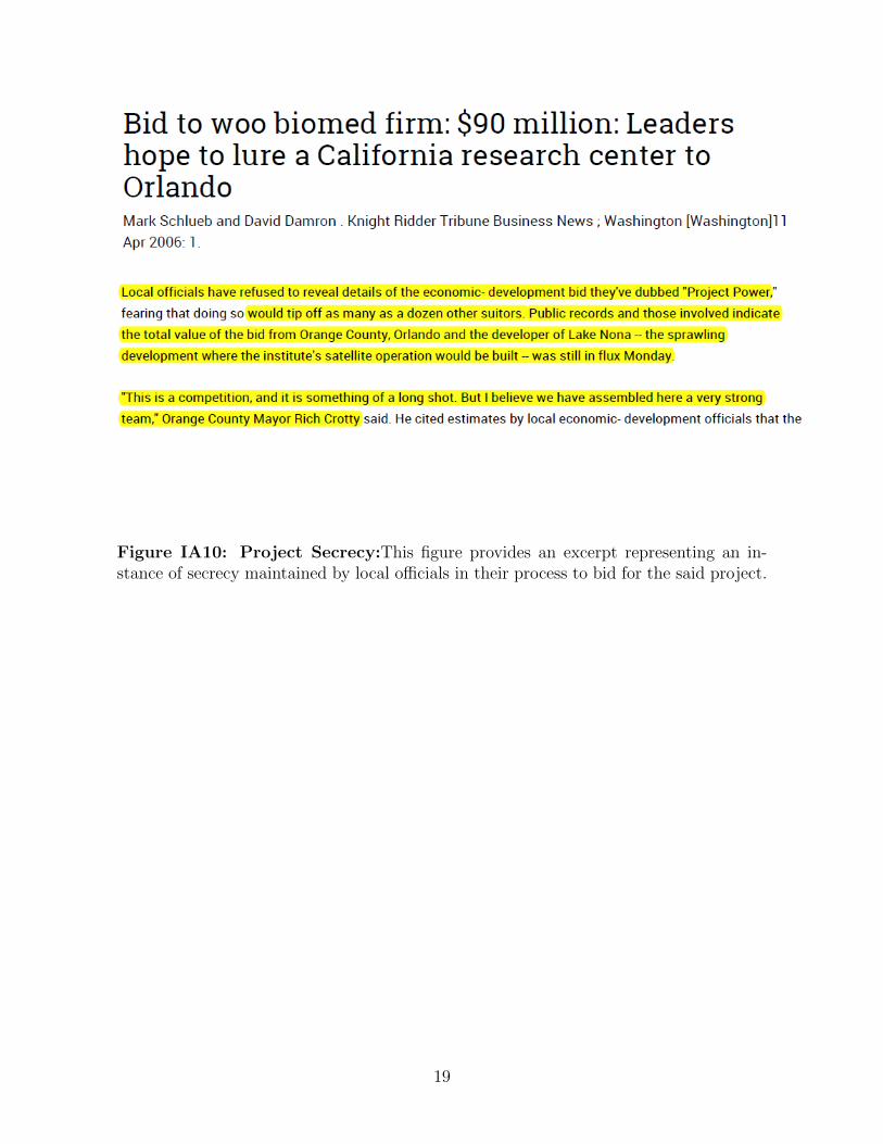
Figure IA10: Project Secrecy:This figure provides an excerpt representing an in-stance of secrecy maintained by local officials in their process to bid for the said project.

19

Table A1: Description of Key Variables

This table reports variable definitions. Data sources include the municipal bond transaction data from

the Municipal Security Rulemaking Board (MSRB), FTSE Russell’s Municipal Bond Securities Database

(FTSE, formerly known as Mergent MBSD), zero coupon yield provided by FEDS, highest income tax

bracket for the corresponding state of the bond issuer from the Federation of Tax Administrators (FTA),

Census data from the Census Bureau Annual Survey of Local Government Finances (CLGF), and subsidy

data from Subsidy Tracker which was enhanced through hand-collection (ST-HC).

Variable Description Source

Winner Dummy set to one for a county that ultimately

wins the subsidy deal. This dummy equals zero

for the runner-up county in that subsidy deal.

ST-HC

Post Dummy that is assigned a value of one for months

after the deal is announced and zero otherwise.

ST-HC, MSRB

Average Yield Volume-weighted average yield for a CUSIP in a

given month. Volume refers to the par value of

the trade.

MSRB

Yield Spread Calculated as the difference between the Average

Yield and the risk free rate. We use the maturity

matched zero coupon yields as the benchmark

for risk free rate following Gurkaynak, Sack, and

Wright (2007).

MSRB, FEDS

After-tax Yield Spread Calculated as the difference between the tax-

adjusted Average Yield and the risk free rate.

We use the maturity matched zero coupon yields

as the benchmark for risk free rate following

Gurkaynak, Sack, and Wright (2007). We follow

Schwert (2017) in applying the tax adjustment.

It is calculated as below:

spreadi,t =yi,t

(1 − τ fedt ) ∗ (1 − τ states,t ))− rt

MSRB, FEDS, FTA

Competitive Bond Dummy Dummy variable that equals 1 if the issue is sold

to underwriters on a competitive basis, and is 0

otherwise

FTSE

20

Variable Description Source

GO Bond Dummy Dummy variable for general obligation bond. A

GO bond is a municipal bond backed by the

credit and taxing power of the issuing jurisdic-

tion rather than the revenue from a given project.

FTSE

Log(Amount) Log transformation of the dollar amount of the

individual bond’s (9-digit CUSIP) original offer-

ing.

FTSE

Callable Dummy Dummy variable that equals 1 if the issue is

callable, and is 0 otherwise.

FTSE

Insured Dummy Dummy variable that equals 1 if the issue is in-

sured, and is 0 otherwise.

FTSE

Remaining Maturity Individual bond maturity measured in years. FTSE, MSRB

Inverse Maturity Inverse of the value of Remaining Maturity ; to

account for non-linearity.

FTSE, MSRB

Interest burden Ratio of interest on general debt to total revenue

for the county.

CLGF

Interest to debt Ratio of interest on general debt to total long

term debt outstanding for the county.

CLGF

Interest to expenses Ratio of interest on general debt to total expen-

diture for the county.

CLGF

Tax privilege The highest state income tax rate applied to

income from municipal bonds issued by other

states minus the highest state income tax rate

applied to income from the winning state-issued

municipal bonds.

FTA

Tax privilege gap Difference in tax privilege between the winning

and losing counties. The tax privilege gap results

from these counties belonging to different states.

FTA

21