Impact of Coordinator Mobility on the throughput in

a Zigbee Mesh Networks Harsh Dhaka

Computer Science and Engineering

Department

Thapar University

Patiala

Atishay Jain Computer Science and Engineering

Department

Thapar University

Patiala

Karun Verma Computer Science and Engineering

Department

Thapar University

Patiala

Abstract— Zigbee (IEEE 802.15.4) standard interconnects simple,

low power and low processing capability wireless devices. The

Zigbee devices facilitate numerous applications such as pervasive

computing, national security, monitoring and control etc. An

effective positioning of nodes in a ZigBee network is particularly

important in improving the performance (e.g., throughput) of

ZigBee networks. In the wireless sensor network (WSN)

literature, the use of a mobile sink is often recommended as an

effective defense against the so-called hot-spot phenomenon. But

the effects of mobile coordinator on the performance of the

network are not given due consideration. In this paper, we

perform extensive evaluation, using OPNET Modeler, to study

the impact of coordinator mobility on ZigBee mesh network. The

results show that the ZigBee mesh routing algorithm exhibits

significant performance difference when the router are placed at

different locations and the trajectories of coordinator are varied.

We also show that the status of ACK in the packet also plays a

critical role in deciding network performances.

Keywords-Sensor Networks; Zigbee; Mobile Coordinator

I. INTRODUCTION

The conventional wireless sensor network (WSN)

architecture consists of a large number of devices (wireless

sensor nodes) at the bottommost layer. On top of these devices

there is a subsystem which supports the routing of the data

from the node to the gateway. The wireless sensor nodes are

miniature battery powered devices with very less power

consumption rates making them appropriate for use in the

remote areas. These sensor nodes are distributed randomly in

area and connected to the outside world through a gateway. A

sensor can act as a Full Functional Device (FFD) or a Reduced

Functional Device (RFD) [8], with at least one FFD acting as a

Coordinator. The primary goal of the RFDs (end devices) is to

gather the data from the surrounding environment and route it

to the coordinator which has superior computing capabilities

and serves as gateway for the entire network. This type of setup

with multiple nodes sending data to a single processing unit are

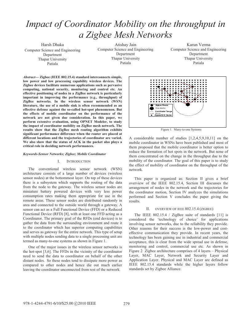
termed as many-to-one systems as shown in Figure 1.

One of the major issues in the wireless sensor networks is

the hot-spot [3,6]. The FFDs in the vicinity of the coordinator

need to send the data to coordinator on behalf of the other

distant nodes. So these nodes tend to dissipate more power as

compared to other nodes and hence die out much earlier

leaving the coordinator unconnected from rest of the network.

Figure 1. Many-to-one Systems

A considerable number of studies [1,2,4,5,9,10,11] on the

mobile coordinator in WSNs have been published and most of

them proposed that the mobile coordinator is better option to

reduce the formation of hot spots in the network. But none of

them concentrated on the change in the throughput due to the

mobility of the coordinator. The goal of this paper is to study

the effect of mobility of coordinator on the throughput of the

network.

This paper is organized as: Section II gives a brief

overview of the IEEE 802.15.4, Section III discusses the

arrangement of nodes in the network and the trajectories for

the coordinator motion, Section IV analyzes the simulations

performed and Section V concludes the paper giving the

results.

II. OVERVIEW OF IEEE 802.15.4 (ZIGBEE)

The IEEE 802.15.4 / ZigBee suite of standards [11] is

considered the ‘technology of choice’ for applications

involving sensor networks, due to the reliability they provide.

Other reasons for their success is the low-power and cost-

effective communication they provide. In recent years, the

technology has been gaining use in industrial and commercial

acceptance, this is clear from the wide spread use in defense,

monitoring and control, commercial use etc. As shown in

Figure 2 Zigbee architecture comprises of 4 layers – Physical

Layer, MAC Layer, Network and Security Layer and

Application Layer. Physical and MAC Layer are defined as

IEEE 802.15.4 standards while the higher layers follow

standards set by Zigbee Alliance.

279978-1-4244-4791-6/10/$25.00 c©2010 IEEE

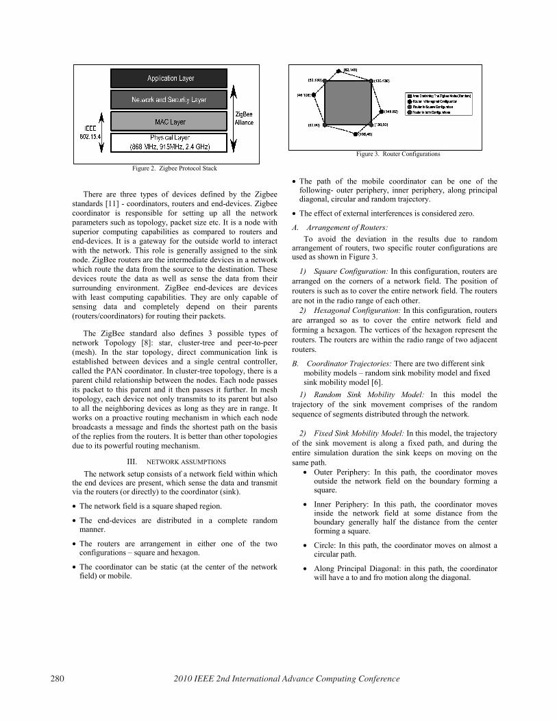
Figure 2. Zigbee Protocol Stack

There are three types of devices defined by the Zigbee standards [11] - coordinators, routers and end-devices. Zigbee coordinator is responsible for setting up all the network parameters such as topology, packet size etc. It is a node with superior computing capabilities as compared to routers and end-devices. It is a gateway for the outside world to interact with the network. This role is generally assigned to the sink node. ZigBee routers are the intermediate devices in a network which route the data from the source to the destination. These devices route the data as well as sense the data from their surrounding environment. ZigBee end-devices are devices with least computing capabilities. They are only capable of sensing data and completely depend on their parents (routers/coordinators) for routing their packets.

The ZigBee standard also defines 3 possible types of network Topology [8]: star, cluster-tree and peer-to-peer (mesh). In the star topology, direct communication link is established between devices and a single central controller, called the PAN coordinator. In cluster-tree topology, there is a parent child relationship between the nodes. Each node passes its packet to this parent and it then passes it further. In mesh topology, each device not only transmits to its parent but also to all the neighboring devices as long as they are in range. It works on a proactive routing mechanism in which each node broadcasts a message and finds the shortest path on the basis of the replies from the routers. It is better than other topologies due to its powerful routing mechanism.

III. NETWORK ASSUMPTIONS

The network setup consists of a network field within which the end devices are present, which sense the data and transmit via the routers (or directly) to the coordinator (sink).

• The network field is a square shaped region.

• The end-devices are distributed in a complete random manner.

• The routers are arrangement in either one of the two configurations – square and hexagon.

• The coordinator can be static (at the center of the network field) or mobile.

Figure 3. Router Configurations

• The path of the mobile coordinator can be one of the following- outer periphery, inner periphery, along principal diagonal, circular and random trajectory.

• The effect of external interferences is considered zero.

A. Arrangement of Routers: To avoid the deviation in the results due to random

arrangement of routers, two specific router configurations are used as shown in Figure 3.

1) Square Configuration: In this configuration, routers are arranged on the corners of a network field. The position of routers is such as to cover the entire network field. The routers are not in the radio range of each other.

2) Hexagonal Configuration: In this configuration, routers are arranged so as to cover the entire network field and forming a hexagon. The vertices of the hexagon represent the routers. The routers are within the radio range of two adjacent routers.

B. Coordinator Trajectories: There are two different sink mobility models – random sink mobility model and fixed sink mobility model [6].

1) Random Sink Mobility Model: In this model the trajectory of the sink movement comprises of the random sequence of segments distributed through the network.

2) Fixed Sink Mobility Model: In this model, the trajectory of the sink movement is along a fixed path, and during the entire simulation duration the sink keeps on moving on the same path.

• Outer Periphery: In this path, the coordinator moves outside the network field on the boundary forming a square.

• Inner Periphery: In this path, the coordinator moves inside the network field at some distance from the boundary generally half the distance from the center forming a square.

• Circle: In this path, the coordinator moves on almost a circular path.

• Along Principal Diagonal: in this path, the coordinator will have a to and fro motion along the diagonal.

280 2010 IEEE 2nd International Advance Computing Conference

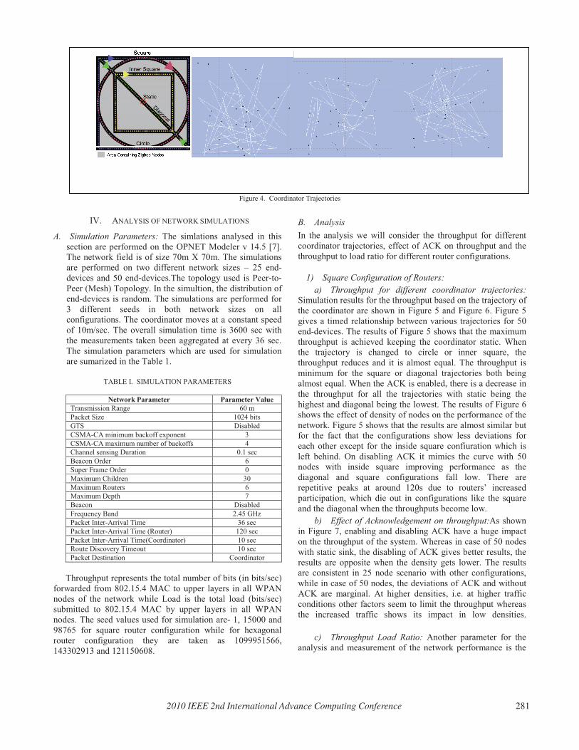
Figure 4. Coordinator Trajectories

IV. ANALYSIS OF NETWORK SIMULATIONS

A. Simulation Parameters: The simlations analysed in this

section are performed on the OPNET Modeler v 14.5 [7].

The network field is of size 70m X 70m. The simulations

are performed on two different network sizes – 25 end-

devices and 50 end-devices.The topology used is Peer-to-

Peer (Mesh) Topology. In the simultion, the distribution of

end-devices is random. The simulations are performed for

3 different seeds in both network sizes on all

configurations. The coordinator moves at a constant speed

of 10m/sec. The overall simulation time is 3600 sec with

the measurements taken been aggregated at every 36 sec.

The simulation parameters which are used for simulation

are sumarized in the Table 1.

TABLE I. SIMULATION PARAMETERS

Network Parameter Parameter Value

Transmission Range 60 m

Packet Size 1024 bits

GTS Disabled

CSMA-CA minimum backoff exponent 3

CSMA-CA maximum number of backoffs 4

Channel sensing Duration 0.1 sec

Beacon Order 6

Super Frame Order 0

Maximum Children 30

Maximum Routers 6

Maximum Depth 7

Beacon Disabled

Frequency Band 2.45 GHz

Packet Inter-Arrival Time 36 sec

Packet Inter-Arrival Time (Router) 120 sec

Packet Inter-Arrival Time(Coordinator) 10 sec

Route Discovery Timeout 10 sec

Packet Destination Coordinator

Throughput represents the total number of bits (in bits/sec)

forwarded from 802.15.4 MAC to upper layers in all WPAN

nodes of the network while Load is the total load (bits/sec)

submitted to 802.15.4 MAC by upper layers in all WPAN

nodes. The seed values used for simulation are- 1, 15000 and

98765 for square router configuration while for hexagonal

router configuration they are taken as 1099951566,

143302913 and 121150608.

B. Analysis

In the analysis we will consider the throughput for different

coordinator trajectories, effect of ACK on throughput and the

throughput to load ratio for different router configurations.

1) Square Configuration of Routers:

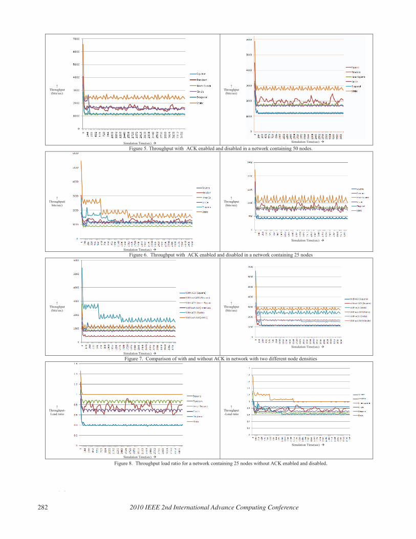
a) Throughput for different coordinator trajectories: Simulation results for the throughput based on the trajectory of

the coordinator are shown in Figure 5 and Figure 6. Figure 5

gives a timed relationship between various trajectories for 50

end-devices. The results of Figure 5 shows that the maximum

throughput is achieved keeping the coordinator static. When

the trajectory is changed to circle or inner square, the

throughput reduces and it is almost equal. The throughput is

minimum for the square or diagonal trajectories both being

almost equal. When the ACK is enabled, there is a decrease in

the throughput for all the trajectories with static being the

highest and diagonal being the lowest. The results of Figure 6

shows the effect of density of nodes on the performance of the

network. Figure 5 shows that the results are almost similar but

for the fact that the configurations show less deviations for

each other except for the inside square confiuration which is

left behind. On disabling ACK it mimics the curve with 50

nodes with inside square improving performance as the

diagonal and square configurations fall low. There are

repetitive peaks at around 120s due to routers’ increased

participation, which die out in configurations like the square

and the diagonal when the throughputs become low.

b) Effect of Acknowledgement on throughput:As shown

in Figure 7, enabling and disabling ACK have a huge impact

on the throughput of the system. Whereas in case of 50 nodes

with static sink, the disabling of ACK gives better results, the

results are opposite when the density gets lower. The results

are consistent in 25 node scenario with other configurations,

while in case of 50 nodes, the deviations of ACK and without

ACK are marginal. At higher densities, i.e. at higher traffic

conditions other factors seem to limit the throughput whereas

the increased traffic shows its impact in low densities.

c) Throughput Load Ratio: Another parameter for the

analysis and measurement of the network performance is the

2010 IEEE 2nd International Advance Computing Conference 281

throughput to load ratio which should be close to one. The

�

Throughput (bits/sec)

Simulation Time(sec) �

�

Throughput(bits/sec)

Simulation Time(sec) �

Figure 5. Throughput with ACK enabled and disabled in a network containing 50 nodes.

�

Throughput(

bits/sec)

Simulation Time(sec) �

�

Throughput

(bits/sec)

Simulation Time(sec) �

Figure 6. Throughput with ACK enabled and disabled in a network containing 25 nodes

�

Throughput

(bits/sec)

Simulation Time(sec) �

�

Throughput

(bits/sec)

Simulation Time(sec) �

Figure 7. Comparison of with and without ACK in network with two different node densities

�

Throughput-

Load ratio

Simulation Time(sec) �

�

Throughput

-Load ratio

Simulation Time(sec) �

Figure 8. Throughput load ratio for a network containing 25 nodes without ACK enabled and disabled.

282 2010 IEEE 2nd International Advance Computing Conference

deviations imply loss of packets while transmision. Figure 8

show the ratios for various configurations. The static sink

configuration has a near perfect ratio, with a higher than one

ratio for 25 nodes due to two devices reading and forwarding

the same packet(directly to sink and via router). Diagonal

again has the worst performance due to inability to get packets

from the opposite end routers most of the time, while it varies

between 0.6 to 0.9 for others with ACK improving

performances of diagonal and square considerably.

2) Hexagonal Configuration of Routers:

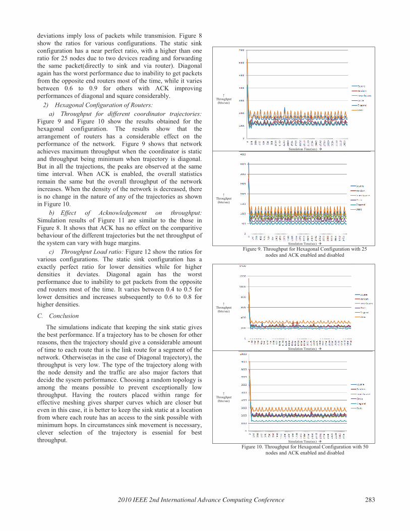
a) Throughput for different coordinator trajectories:

Figure 9 and Figure 10 show the results obtained for the

hexagonal configuration. The results show that the

arrangement of routers has a considerable effect on the

performance of the network. Figure 9 shows that network

achieves maximum throughput when the coordinator is static

and throughput being minimum when trajectory is diagonal.

But in all the trajections, the peaks are observed at the same

time interval. When ACK is enabled, the overall statistics

remain the same but the overall throughput of the network

increases. When the density of the network is decreased, there

is no change in the nature of any of the trajectories as shown

in Figure 10.

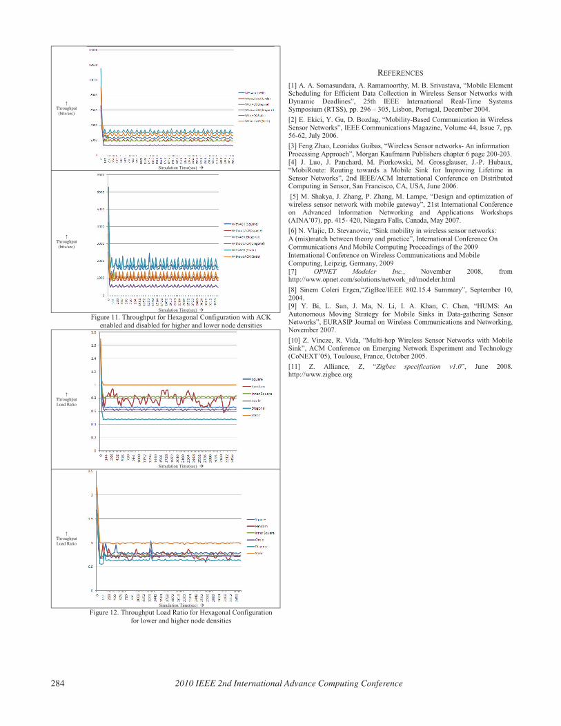
b) Effect of Acknowledgement on throughput:

Simulation results of Figure 11 are similar to the those in

Figure 8. It shows that ACK has no effect on the comparitive

behaviour of the different trajectories but the net throughput of

the system can vary with huge margins.

c) Throughput Load ratio: Figure 12 show the ratios for

various configurations. The static sink configuration has a

exactly perfect ratio for lower densities while for higher

densities it deviates. Diagonal again has the worst

performance due to inability to get packets from the opposite

end routers most of the time. It varies between 0.4 to 0.5 for

lower densities and increases subsequently to 0.6 to 0.8 for

higher densities.

C. Conclusion

The simulations indicate that keeping the sink static gives

the best performance. If a trajectory has to be chosen for other

reasons, then the trajectory should give a considerable amount

of time to each route that is the link route for a segment of the

network. Otherwise(as in the case of Diagonal trajectory), the

throughput is very low. The type of the trajectory along with

the node density and the traffic are also major factors that

decide the sysem performance. Choosing a random topology is

among the means possible to prevent exceptionally low

throughput. Having the routers placed within range for

effective meshing gives sharper curves which are closer but

even in this case, it is better to keep the sink static at a location

from where each route has an access to the sink possible with

minimum hops. In circumstances sink movement is necessary,

clever selection of the trajectory is essenial for best

throughput.

�

Throughput (bits/sec)

Simulation Time(sec) �

�

Throughput

(bits/sec)

Simulation Time(sec) �

Figure 9. Throughput for Hexagonal Configuration with 25

nodes and ACK enabled and disabled

�

Throughput

(bits/sec)

Simulation Time(sec) �

�

Throughput

(bits/sec)

Simulation Time(sec) �

Figure 10. Throughput for Hexagonal Configuration with 50

nodes and ACK enabled and disabled

2010 IEEE 2nd International Advance Computing Conference 283

REFERENCES

[1] A. A. Somasundara, A. Ramamoorthy, M. B. Srivastava, “Mobile Element Scheduling for Efficient Data Collection in Wireless Sensor Networks with Dynamic Deadlines”, 25th IEEE International Real-Time Systems Symposium (RTSS), pp. 296 – 305, Lisbon, Portugal, December 2004.

[2] E. Ekici, Y. Gu, D. Bozdag, “Mobility-Based Communication in Wireless Sensor Networks”, IEEE Communications Magazine, Volume 44, Issue 7, pp. 56-62, July 2006.

[3] Feng Zhao, Leonidas Guibas, “Wireless Sensor networks- An information Processing Approach”, Morgan Kaufmann Publishers chapter 6 page 200-203.

[4] J. Luo, J. Panchard, M. Piorkowski, M. Grossglauser, J.-P. Hubaux, “MobiRoute: Routing towards a Mobile Sink for Improving Lifetime in Sensor Networks”, 2nd IEEE/ACM International Conference on Distributed Computing in Sensor, San Francisco, CA, USA, June 2006.

[5] M. Shakya, J. Zhang, P. Zhang, M. Lampe, “Design and optimization of wireless sensor network with mobile gateway”, 21st International Conference on Advanced Information Networking and Applications Workshops (AINA’07), pp. 415- 420, Niagara Falls, Canada, May 2007.

[6] N. Vlajic, D. Stevanovic, “Sink mobility in wireless sensor networks: A (mis)match between theory and practice”, International Conference On

Communications And Mobile Computing Proceedings of the 2009

International Conference on Wireless Communications and Mobile Computing, Leipzig, Germany, 2009

[7] OPNET Modeler Inc., November 2008, from http://www.opnet.com/solutions/network_rd/modeler.html

[8] Sinem Coleri Ergen,“ZigBee/IEEE 802.15.4 Summary”, September 10,

2004. [9] Y. Bi, L. Sun, J. Ma, N. Li, I. A. Khan, C. Chen, “HUMS: An Autonomous Moving Strategy for Mobile Sinks in Data-gathering Sensor Networks”, EURASIP Journal on Wireless Communications and Networking, November 2007.

[10] Z. Vincze, R. Vida, “Multi-hop Wireless Sensor Networks with Mobile Sink”, ACM Conference on Emerging Network Experiment and Technology (CoNEXT’05), Toulouse, France, October 2005.

[11] Z. Alliance, Z, “Zigbee specification v1.0”, June 2008. http://www.zigbee.org

�

Throughput

(bits/sec)

Simulation Time(sec) �

�

Throughput

(bits/sec)

Simulation Time(sec) �

Figure 11. Throughput for Hexagonal Configuration with ACK

enabled and disabled for higher and lower node densities

�

Throughput

Load Ratio

Simulation Time(sec) �

�

Throughput

Load Ratio

Simulation Time(sec) �

Figure 12. Throughput Load Ratio for Hexagonal Configuration

for lower and higher node densities

284 2010 IEEE 2nd International Advance Computing Conference