IMPACT OF CHANGES IN MARRIAGE LAW: IMPLICATIONS FOR FERTILITY AND SCHOOL … · 2014-08-16 · IMPACT OF CHANGES IN MARRIAGE LAW: IMPLICATIONS FOR FERTILITY AND SCHOOL ENROLLMENT

IMPACT OF CHANGES IN MARRIAGE LAW: IMPLICATIONS FOR FERTILITYAND SCHOOL ENROLLMENT

PRASHANT BHARADWAJ †

ABSTRACT. Does the postponement of marriage affect fertility and investment in human capital?

I study this question in the context of a 1957 amendment to the marriage law in Mississippi that

was aimed at delaying the age of marriage; changes included raising the minimum age for men and

women, parental consent requirements, compulsory blood tests and proof of age. Using a difference-

in-differences design at the county level, I find that overall marriages per 1000 in the population

in Mississippi and its neighboring counties decreased by nearly 75%; crude birth rate decreased

between 2-6%; and school enrollment increased by 3% after the law was enacted (by 1960). An

unintended consequence of the law change was that illegitimate births among young black mothers

increased by 7%. I show that changes in labor market conditions during this period cannot explain

the changes in marriages, births and enrollment. I conclude that stricter marriage-related regulation

leading to a delay in marriage can postpone fertility and increase school enrollment.

† DEPARTMENT OF ECONOMICS, UNIVERSITY OF CALIFORNIA SAN DIEGOE-mail address: [email protected].

Much thanks to Achyuta Adhvaryu, Joseph Altonji, Michael Boozer, Julie Cullen, Gordon Dahl, Roger Gordon,Fabian Lange, Paul Niehaus and Ebonya Washington for comments on earlier versions of this paper. Dick Johnsonwas instrumental in obtaining historical data from Mississippi. Hrithik Bansal, Karina Litvak and Taylor Marvinprovided excellent research assistance. This version: June 2014.

1

2 BHARADWAJ

1. INTRODUCTION

The decision of when to marry has important consequences for men and women. Particu-

larly for women, early marriage is often associated with lower socio-economic status and schooling

(Dahl 2009, Field & Ambrus 2006). Marital status is also known to be an important determinant

of female labor force participation (Angrist & Evans 1996, Heckman & McCurdy 1980, Stevenson

2008); moreover, women seem to invest more in their careers if they delay fertility and marriage

(Goldin & Katz 2002). It is clear that women’s (and to some extent men’s) marital decisions are

intricately tied to their economic outcomes. While marriage is considered a choice, laws regard-

ing marriage often control various aspects of who marries, when people marry, partner choice and

number of partners. Moreover, societal norms place importance on the act of marriage to legit-

imize co-habitation and childbearing. In the US, for example, married couples form 90% of all

heterosexual couples (US census Report 2007)1 and the majority of children born are to married

couples (Hamilton et al, 2005). Given the central role of marriage (78% of all women above the

age of 18 ever marry), marriage laws can have direct implications for the economic outcomes of

men and women.

Marriage laws can be used as a policy tool as well - in 1980 China raised the age of

marriage for women in a bid to control fertility. On the other hand, if legal marriage is just a

formality or if marriage laws are routinely ignored,2 then it is likely that changes in marriage law

will not have much of an impact. Given the intended policy goals of marriage laws as well as rising

cohabitation rates, an important, empirical question surrounding marriage laws is whether changes

in marriage laws, particularly changes that raise the cost of marriage, have an impact on marriage

rates, fertility and schooling. Fertility and schooling reflect key investments that men and women

make early on in their adult lives that have long term consequences for welfare and labor market

1While rates of co-habitation have been on the rise in the US, demographic evidence suggests that it is not becominga substitute to marriage (Raley 2001).2A case in point is the change in marriage law in India in 1978 which raised the minimum age of marriage. The ChildMarriage Restraint Act of 1978 increased the age of marriage for women from 15 to 18, however, the data shows nosharp breaks around this time period in the age at which women got married. Moreover, survey data evidence showsthat awareness of these marriage laws is also weak in the Indian context.

IMPACT OF CHANGES IN MARRIAGE LAW 3

outcomes; hence, from a policy perspective it is relevant to know whether and how marriage laws

affect these investments.

While many recent papers have examined the consequences of divorce laws,3 few have

studied the impact of marriage law changes on outcomes such as fertility and schooling. Dahl

(2009) uses marriage law changes as an instrument for delayed marriage to study the relationship

between early teen marriage and poverty. However, Dahl uses marriage law changes along with

schooling changes to analyze the impact of both laws simultaneously as changes in compulsory

schooling laws often coincide with changes in marriage laws. Buckles, Guldi and Price (2009)

examine the role played by blood test requirements for obtaining marriage licenses, and find that

even small increases to the cost of marriage can decrease marriage rates and increase the incidence

of illegitimate births. Finally, Blank, Charles and Sallee (2009) find evidence of misreporting of

age in marriage licenses, and find that young men and women tend to avoid restrictive marriage

laws by getting married in a different state. This paper adds to this body of work by examining not

only the effect of changes in marriage laws on marriage rates, but also on fertility and educational

investments. While this paper examines the impact of a wide range of marriage law changes,

the results make it clear that the age restrictions perhaps have the largest impact. Hence, this

paper complements Buckles, Guldi and Price (2009) in showcasing another aspect of marriage law

changes and its impact on a wide range of policy relevant outcomes.

A priori, it is not clear what effect increasing barriers to marriage will have on fertility

and schooling. If entering into marriage becomes harder, individuals may simply have children

out of wedlock, exacerbating the problem since then the father is less likely to help raise the child.

After marriage, the sharing of resources becomes easier, hence spouses may also be more likely to

have a chance to get further education – so, the postponement of marriage could reduce education

(Stevenson (2007) shows that divorce laws negatively impact spousal support for education related

investments). Alternatively, if people are reluctant to have children out of wedlock, postponement

of marriage could lead to a drop in the birth rate. Moreover, unmarried women lacking spousal

3Stevenson (2007, 2008), Stevenson and Wolfers (2006), Rasul (2006) are some of the many papers that considerthe impact of divorce laws on various outcomes like fertility, education, marriage quality, and incidences of domesticviolence.

4 BHARADWAJ

support might have more incentives to invest in their own education - hence marriage laws could

increase school enrollment and educational attainment. Hence, the impact of changes in marriage

law is essentially an empirical question.

In 1957, the state of Mississippi amended its marriage law. The changes included an

increase in the minimum marriage age for women from 12 to 15 years and for men from 14 to 17

years. The law also introduced a parental consent requirement if either party was under the age of

18, a compulsory three day waiting period, serological blood tests and proof of age. In addition,

brides under the age of 21 were required to marry in their county of residence. Hence, the barriers

to marriage were raised not just via increasing minimum age laws but also by introducing blood

tests and other requirements, affected everyone. Using a difference-in-differences strategy that

considers Mississippi and its surrounding counties as the treatment group and remaining counties

in the states neighboring Mississippi (Alabama, Louisiana, Arkansas and Tennessee) as the control

group, I find that by 1960, marriages per 1000 had decreased by 75%, crude birth rate (births per

1000 in the population) decreased between 2-6%, and enrollment among 14-17 year olds increased

by 3% more than the corresponding change in the control group. Using yearly state-level data from

1952 to 1960, I find that the percentage of total births born to young black women decreased by

8%, and similarly for white women, the decline was 18% more than the change in the control

group. However, this decrease in births is mitigated by an increase in illegitimate births, primarily

among black women.

I focus on short run effects of the law change as there were tremendous social and eco-

nomic changes in the 1960s - in particular due to the Civil Rights Act of 1964 - that could confound

an analysis of long run outcomes. Moreover, the 1960s and 1970s saw the introduction of vari-

ous contraceptives (the birth control pill in particular), the legalization of abortion, and changes in

divorce laws, which could also affect marriage and fertility (Goldin and Katz 2002, Donohue &

Levitt 2001, Ananat and Hungerman 2011, Bailey 2006). With this caveat in place, using the 1990

census I do not find long run effects on fertility, suggesting that the drop in birth rates is simply


a delay in fertility.4 I do find that women affected by the law were more likely to complete high

school in the long run.

This paper’s relevance extends to the context of developing countries, where age at first

marriage and educational attainment of women tend to be quite low. Therefore, for women in

developing countries who have high levels of fertility and low levels of educational attainment,

laws that delay marriage might be welfare improving. Field and Ambrus (2008) show that women

who marry later attain more years of education in Bangladesh. Given this finding, they hypothesize

that imposing universal age of consent laws can raise educational levels of women. The findings

of this paper provides direct corroborating evidence towards this idea, albeit in the setting of the

American South. Marriage laws are also thought of as a tool for reducing fertility. The results of

this paper suggest that raising the minimum age of marriage delays fertility but perhaps has little

effect on completed fertility.

2. BACKGROUND AND PRELIMINARY EVIDENCE OF MARRIAGE DECLINE

In 1957, the state of Mississippi amended its existing marriage laws. A Time magazine

article from December 1957 carried a prediction that the proposed changes in marriage law would

"shoot out loveland’s neon lights and keep rash child brides at home". In particular, the article

mentions that, due to lenient laws in Mississippi compared to its neighboring states, the state’s

border counties were a haven for early marriages. Changes in Mississippi’s marriage laws were

driven by "increased pressure from physicians, ministers and clubwomen". The changes included

raising the minimum age of marriage for women from 12 to 15, for men from 14 to 17, and

introducing parental consent laws. Circuit clerks were required to notify the parents of minors via

registered mail during the mandatory three day waiting period (which was also introduced at the

same time). Age verification and blood tests were additional requirements that were added to the

existing laws.

Did these changes lead to a decline in marriages? To answer this question, I begin by

summarizing some of the findings of Plateris (1966), who first examined the impact of this law

4This is in contrast to an earlier version of the Field and Amrbus (2006) paper, Field (2004) where a delay in marriageis found to have a sizable but barely significant impact on completed fertility.

6 BHARADWAJ

change on marriage rates. I also present additional evidence of the marriage decline using data

from the Vital Statistics and the City and County Handbooks (section 3 describes the data used in

this paper in detail). The evidence I present here is largely graphical and the econometric evidence

is presented later in the paper.

While the marriage law amendment was passed in 1957, it went into effect in 1958 and

immediately resulted in a substantial decline in marriages performed in Mississippi. The result-

ing decline in Mississippi was a combination of a decline from out of state couples and in state

couples who did not meet the requirements. Indeed, Mississippi’s laws prior to 1958 were lenient

in comparison to its surrounding states of Alabama, Arkansas, Louisiana and Tennessee. Figure

2 uses yearly marriage rates from the Vital Statistics to show the decline in Mississippi relative

to its surrounding states. Importantly, it shows that while marriages in Mississippi declined and

marriages in surrounding states increased, in no way was the increase enough to compensate for

the massive decline. Plateris (1966) uses state of residence information from the Mississippi State

Board of Health to confirm this (see Appendix Table 1).5 From 1957 to 1959, Plateris (1966) notes

that marriages in Mississippi where both spouses resided in the state declined by 20%, while mar-

riages in Mississippi where both spouses were non-residents of Mississippi declined by 90%. As

a result, most of the decline in Mississippi itself was driven by the drop in out of state marriages.

Out of state couples who did not get married in Mississippi could still get married in their home

state and many did so. However, even taking the increase in marriages in neighboring states into

account, the area in general saw a decline in the number of marriages by 13%. I confirm these

findings using county level marriage data and plotting changes in marriage rates between 1950-54

and 1954-1960. Figures 3a and 3b clearly show a large decline after the law change in counties

that were closer to the Mississippi border (in particular along the Mississippi-Alabama border).

As further evidence, Figure 4a shows the drop in marriages at the state-level using census

data from 1930 through 1970. This figure is also useful in seeing that before 1950 we do not see

any Mississippi specific trends in marriages. In fact, between 1930 and 1950 trends in marriage in

Mississippi looked very similar to trends in its neighboring states as well as other Southern states.

5Appendix Tables are available at http://prbharadwaj.wordpress.com/papers/


After 1950, however, we see that the proportion of married 19-year-olds (they were 16-17 when the

law was passed) in Mississippi drops sharply, below that of all other states. Figure 4b uses age of

marriage data from the 1960 and 1970 census to compute the fraction of married teenagers. While

this figure is predictably noisier, the decline in marriage in Mississippi is apparent. Importantly,

these graphs show why a difference-in-differences approach is needed - the proportion of married

19-year-olds, or the fraction of married teenagers in other states, also seems to have declined in the

late 1950s; hence, it will be crucial to separate the decline due to the secular trend from the decline

due to the marriage law.

3. DATA AND EMPIRICAL STRATEGY

Isolating the impact of the change in marriage law is a critical challenge in this case. It is

likely that changes in schooling and fertility of women is caused by local and/or macro conditions

unrelated to the change in marriage law. The main strategy used to differentiate the effect of the law

from other causes in this paper is a difference-in-differences strategy; however, data limitations for

certain outcomes and years determine the type of difference-in-differences strategy used. Critical

for my strategy, neighboring states of Mississippi did not experience a change in marriage law

during this period (1950-1960), and no state considered for the analysis experienced a change in

compulsory schooling laws. Moreover, Arkansas, Tennessee and Louisiana’s minimum marriage

age for women was 16, while Alabama’s was 14 during 1950-1960. In fact, Mississippi was the

only state in the country during this decade to have the minimum age at 12 for women - all states

had a higher minimum age by 1950.6

One of the main challenges while using a difference-in-differences strategy is to appro-

priately define treatment and control groups. Section 2 suggests a few different ways to define

treatment and control groups. The definition of treatment is based largely on the degree of data

disaggregation available. Using county level data, we can use distance from the Mississippi border

as a continuous measure of treatment or Mississippi and its surrounding counties as treatment and

remaining counties in the neighboring states as control as a dichotomous measure of the areas that6One might worry about migration out of Mississippi to get married after the change in law, especially to Alabamasince the minimum age there was less than Mississippi after 1957. However, we know from Plateris (1966) that thiswas not very prevalent who reports a net decline of 20% for Mississippi resident marriages.

8 BHARADWAJ

were affected by the law change (as suggested by Figure 3). Using state-level data, we can use

Mississippi and neighboring states as treatment and remaining southern states (where Southern is

defined as a census region) as the control, for example. In addition, the nature of the law change

implies that younger age groups should be more affected than older age groups. The age dimension

of the law changes allows for a triple difference strategy; i.e. comparing younger and older age

groups across treatment and control states before and after the law change.

However, as I explain below, some of these strategies cannot be used in conjunction due to

data limitations. Importantly, some of the data is available for more years, which allows for a more

accurate control for trends prior to the law change, another aspect of a difference-in-differences

analysis that is quite critical. The subsections below explain in detail the different strategies used.

3.1. County Level Analysis. County level analysis has the distinct advantage that I can examine

changes in border counties relative to interior counties of neighboring states. Specifically, it allows

me to construct treatment groups such that the intensity of "treatment" decreases with distance

away from the Mississippi border. Comparing counties within the same state that only differ by

distance to the Mississippi border reduces the possibility that factors other than the law change in

Mississippi are driving the results. However, this strategy comes at the cost of not being able to

include Mississippi as part of the results. To include Mississippi as part of the treatment group,

I define a more restrictive treatment group comprising counties in Mississippi and counties in

neighboring states that share a border with Mississippi. The remaining counties in neighboring

states comprise the control group under this specification. Evidence from Section 2 suggests that

this is a reasonable way to assign treatment and control. Under this definition of treatment and

control, in some specifications, I can take advantage of using county level data by controlling for

state-by-year trends.7 A major advantage of county level data over census data is that county level

data is available for inter-censal years. Marriage rates, for example, are available for the years

1948, 1950, 1954 and 1960 at the county level, while fertility is available at the yearly level from

1945-1965. This allows me to control accurately for trends prior to the law change.

7Again, doing so would exclude Mississippi counties since all Mississippi counties are defined as a "treated" county.


The disadvantage of using county level data is that the county level data does not contain

details on sex, race or age. In particular data by age would have allowed for sharper analysis

since the minimum age and parental consent laws were directed towards younger age groups. In

sum, the county level analysis yields the preferred set of estimates. While using data by age and

gender is an important check on the validity of the estimates, the advantage of using distance from

the Mississippi border as well as data from inter-censal years and being able to control for state

specific trends is a major advantage of using county level data.

The difference-in-differences strategy using county level data can be estimated as follows:

Outcomeijt = β1Treatijt + β2Postijt + β3(TreatijtXPostijt) + αjt + γXijt + εijt(1)

Where Outcomeijt stands for an outcome like marriage or enrollment rates in county i

in state j at time t. Treatijt denotes whether the county is defined as a "treated" county. In the

case of using distance from the Mississippi border, Treatijt is simply the inverse of distance to the

Mississippi border. An alternative definition of treatment used in this paper is to define all counties

in Mississippi and border counties of neighboring states as treated. In this case, Treatijt is simply

a dummy variable, taking the value of 1 for treated counties and 0 for control counties. Postijt

is dummy variable that takes a value of 1 for years after 1957 and is 0 otherwise. The coefficient

of interest here is β3 which is the difference-in-differences coefficient. Xijt denotes a vector of

controls like tractor use, employment in manufacturing, etc. αit denotes the state-by-year fixed

effect, although I can only use this in cases where Mississippi is not included in the analysis. In

the specifications that include Mississippi, I use state and year fixed effects.8

Due to the inclusion of border counties in neighboring states in the treatment group, stan-

dard errors are clustered at the county level. However, results using different level of clusters is

shown in the Appendix. Bertrand, Duflo and Mullainathan (2004) stress the importance of clus-

tering standard errors while using DD techniques to examine the impact of law changes. Since the

law was imposed at the state-level in Mississippi, an argument could be made that conservative

8This specification is:

Outcomeijt = β1Treatijt + β2Postijt + β3(TreatijtXPostijt) + α1t + α2j + γXijt + εijt

10 BHARADWAJ

standard errors are achieved by clustering at the state-level. However, clustering at the state-level

yields five clusters in my case leading to large standard errors for some of the results. To deal with

small number of clusters, I use three approaches. First, I use the methodology in Buchmueller,

DiNardo and Valleta (2011) of using "placebo" states to obtain the sampling distribution of the

difference-in-differences coefficient. In other words, equation 1 is estimated using other states as

the treated state and the coefficient obtained for Mississippi is compared to the coefficient obtained

for other states. According to Buchmueller, DiNardo and Valleta (2011), this procedure results in

"conservative and appropriate" standard errors. Second, I can increase the number of clusters under

the standard procedure by expanding the control group to counties in Texas, Florida, Oklahoma,

Virginia, West Virginia, Georgia, Kentucky, North Carolina, Delaware and Maryland/Washington

DC. This give me 10 more states to include, increasing the number of clusters to 15. I could also

include all states in the country and increase the number of clusters to 50. In general, different

clustering procedures do not affect the interpretation of the main results. Even under the most

conservative of clustering procedures, most of the results remain statistically significant. Results

with different clustering methods are presented in Appendix Table 2.

County level data for birth rates and enrollment was obtained from the City and County

Handbooks for the years 1948, 1950, 1954 and 1960. Data is not available for the intervening

years. This data is at the county level and contains important demographic (marriage, fertility

and schooling) and labor market related variables (wages, tractor use etc). The City and County

data book get their birth and marriage data from the Vital Statistics. However, not all variables

are present for all years, nor are they necessarily in a format that is comparable across years. For

example, school enrollment in the City and County Handbook is available for age groups 14-17 in

1950, but only for age groups 5-34 in 1960. Hence, school enrollment data at a comparable level

between 1950 and 1960 is obtained from the historical census collection from the University of

Virginia Library website. The historical census provides county identifiers, but as it is a census,


there is no data on enrollment for any intercensal year.9 In addition, I obtained yearly county level

births from 1946-1965 thanks to a data collection effort undertaken by Martha Bailey.10

3.2. State-Level Analysis. Data at the state-level comes from the census and has the advantage

that some of this data contains data by age. Since the law change was intended to affect certain age

groups more than others, using age specific information, I can assign treatment status not only by

state of residence, but also by age. I can do this using census data from 1950 and 1960. Women

below the age of 21 (and particularly below the age of 18) in 1957-1958 were impacted by the

change in marriage law, so women above the age of 21 in 1957 should not be affected by the

change in marriage law, or at the very least should be affected less than women below the age of

21. This is because while proof of age and blood test requirements affected everybody, the age

restrictions were an added barrier for women below the age of 21 in 1960. In addition, verifying

the results using census data is critical in light of potential misreporting of age in marriage licenses

(Blank, Charles and Sallee (2009)). A triple difference-in-differences (essentially a state-cohort

analysis) exploits the age specific impact of the marriage law.

Using 1950 and 1960 census data at the state-level, the estimating equations typically take

the following form:

Yijtg = βg(Treatijtg ∗ Postijtg ∗∑g=33

g=14Aijtg) + γ1(Treatijtg ∗∑g=33

g=14Aijtg) +(2)

γ2(Postijtg ∗∑g=33

g=14Aijtg) + γ3Treatijtg + γ4Postijtg +

γ5∑g=33

g=14Aijtg + υijtg

Where Yijtg is the relevant outcome (age of marriage, school enrollment, number of chil-

dren, etc) for person i in state j at time t belonging to age group g. Treat is a dummy that takes

9The historical censuses also do not have marriages and births by sex, race or age. They simply contain aggregates forthe year 1950 and 1960.10Bailey, Martha J. 2010. 1946-65 County Natality Data for AL, AR, MS, LA, TN. University of Michigan, December31. Data collection funded by the University of Michigan’s National Poverty Center, Robert Wood Johnson Healthand Society Programs, University of Michigan Population Research Center’s Eva Mueller Award, and the NationalInstitute of Health (Grant HD058065-01A1).

12 BHARADWAJ

on 1 if the person lives in Mississippi or its neighboring states and 0 otherwise.11 Post is a dummy

that is 1 if year is 1960 and 0 otherwise. A is a dummy that takes on the value of 1 if the person

belongs to age group g and 0 otherwise. The DD estimate is the triple interaction of Age, Treat

and Post, and all lower interaction terms and main effects are included in the regression. Note that

the interaction of Treat and Post is not included. The inclusion of all age dummies interacted

with Treat and Post implies that the double interaction is completely described by this triple

interaction.

Triple DD estimates are obtained by comparing the β for younger versus older age groups.

Standard errors are clustered at the state-year level. The age groups (as of 1957) are 11-14, 16-20,

21-25 and 26-30. These groupings were made to facilitate presentation of the results and to clearly

show that the main impacts of the marriage law are coming through younger age groups.12 While

the triple interaction for all age groups is included, double interactions and main effects for age

group 26-30 form the excluded group. A key advantage of the census data is that in 1960 the

census asked about age at first marriage for the sample that reports having been married (in 1950,

while they do not ask about age at first marriage, they ask about duration of marriage from which

we can impute the age of marriage for those who report currently being married). Age of marriage

in the census is likely to be more reliable than age of marriage in the Vital Statistics since the Vital

Statistics records age of marriage at the time of marriage when incentives to misreport age might

be higher. In the census, there are no such incentives to misreport.

The disadvantage of using census level data is that there is no data for the inter-censal

years. This limits the extent to which I can control for differential trends in the 1950s. Moreover,

it is difficult to accurately assign treatment status with just state-level identifiers. Since border

counties of neighboring states of Mississippi were also affected, I present results using two versions

of a treatment group. My preferred estimate comes from using just Mississippi and its neighboring

11State of residence from the census is used to assign persons to treatment or control group. Since the law change wasimplemented in 1958, only two years passed between the passage of the law and the 1960 census. In 1960 9% reporthaving lived in a different state in the last 5 years in the treatment group and 12% in the control group. Moreover, themigration rates are much lower for blacks than for white. Only 3% of blacks report having lived in a different state inthe past 5 years in 1960 in the treatment group, while the same statistic for the control group is around 5%. The 1950census does not have comparable migration information.12The groupings per se are not essential to the results - indeed Appendix Table 3 shows very similar results when theage group dummies in equation 2 are replaced with individual age dummies.


states as the treatment group and the remaining states in the southern region (as defined by the

census) as the control group. As a robustness check, I assign only Mississippi as the treatment

group and treat its neighbors as the control group.

As a compromise between the county level data and the census data, I collected data from

the Vital Statistics at the state-level for outcomes such as births and illegitimate births. The state-

level Vital Statistics were available from 1952 onwards and provide yearly information on births

and illegitimate births by age and race of the mother. While I cannot conduct a distance level

analysis with this data, I can estimate equation 1 using Mississippi as the treated state and its

neighbors as the control states for various age groups.

4. RESULTS

This section presents results from estimating equations 1 and 2. Since county level esti-

mates are the preferred estimates, for each outcome I first present county level estimates followed

by state-level estimates.

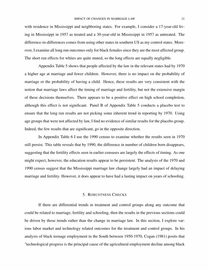
4.1. Marriage decline. While Figures 1-4 largely establish the impact of the law change on mar-

riage rates, this section provides more specific evidence. Using distance to the Mississippi border

as the definition of treatment, Table 2 estimates equation 1 and shows that distance to border mat-

ters for marriage rates after 1957 (the interaction of distance inverse and post dummy), and that

this is a statistically significant effect. In order the make the table interpretable, I use the inverse

of distance to Mississippi border, therefore, the interaction term suggests that places close to the

Mississippi border after the law change experienced an increase in marriages. This confirms the

casual observation in Plateris (1966, replicated in Appendix Table 1) as well as Figure 5. Note,

that this increase does not make up for the overall decrease in number of marriages.

The downside to this definition of treatment is that it necessarily excludes Mississippi

from the analysis. In order to include Mississippi as a treated group, I define Mississippi and

bordering counties as the treatment group, with remaining counties in the neighboring states as the

control group. Table 3 shows estimates of equation 1 with various controls. While the treatment

group definition stays the same (Mississippi and counties in AL, AR, TN and LA that border

14 BHARADWAJ

it), Column 1 uses all southern counties as the control group. Column 2 shows that restricting

the control group to counties in the neighboring states of Mississippi does not change the results

much. In Column 3, I add state and year controls, which again do not make any difference (I can

use state fixed effects as the treatment group consists of counties within states). Columns 4 and

5 add county level controls like manufacturing wages, employment in manufacturing industries,

number of farms and employment in agriculture - these are key labor market related variables and

trends in these variables could affect marriage rates independently of the change in law. Since

agricultural employment was only collected for 1950 and 1960, Column 5 has fewer observations

than Column 4. Comparing coefficients across Columns 1-5 shows that adding controls does not

change the coefficient on the difference-in-differences estimator (the interaction of Treatment and

Post dummies). The results indicate that after the change in law, treatment counties experienced

a drop of 10 marriages per 1000 in the population. Prior to 1957, the marriages per 1000 in

Mississippi and its neighboring counties was around 22 (Table 1). Table 2 shows a remarkable

decline of almost 50% compared to the pre-law change average.

Columns 6 and 7 show the impact of the marriage law when we exclude Mississippi from

the analysis. Because the entire state of Mississippi is part of the treatment group, when I include

state-by-year fixed effects, only the border counties in the neighboring states are identified. Hence,

the DD estimator has a positive sign for these columns. Comparing Column 6 and 7 also shows

that adding state-by-year fixed effects, which controls for state specific trends does not change the

fact that marriage rates were affected by the change in law. This suggests that the DD estimator is

indeed picking up the change in marriages due to the change in law as opposed to changes due to

other differential trends at the state-level.

Moving to state-level analysis using the data from the census, Table 4 shows that for

younger age groups among women, the probability of being married (this is defined throughout

this analysis as being married by the time of the relevant census) decreased and the age of marriage

increased by 1960. This table is created by estimating equation 2 using 5 year age groups instead

of individual age dummies for easy interpretation. The omitted age group is the age group 31-35.

Compared to this age group, Column 6 in Table 2 shows, for example, that black women in the age


group 16-20 as of 1957 experienced an increase in marriage age of nearly 0.4 years. Compared

to the average age of marriage for black women in the sample (19 years), the increase in marriage

age is quite large. The same applies for the probability of being married. Black women in the age

range 16-20 are 13 percentage points less likely to report being married by 1960, representing a

23% change from the mean probability of being married.

Comparing the difference-in-differences coefficient across various age groups, it is clear

that the most impacted age group is the group aged 16-20 in 1957-58, rather than say the age group

of 26-30. This is reassuring as the changes in the marriage law were mainly directed at younger

age groups due to various age restrictions.

Results using census data show that most of the overall effects appear to be driven by

blacks. Blacks formed a large portion of the overall population in the South - by 1960 blacks were

about 26% of the population in Mississippi and its surrounding states (Mississippi’s population at

the time was nearly 51% black). Moreover, among black women, the effect on marriages extends

to the 21-25 age group as well. This is likely due to restrictions like proof of age and blood tests

being a greater burden on blacks than on whites during this time period. This is similar to Buckles,

Guldi and Price (2009), who find that blood test laws for marriages were more of a deterrent to

blacks. Thus, relative to whites, it appears that the marriage law changes in Mississippi raised the

cost of marriage mainly for blacks.

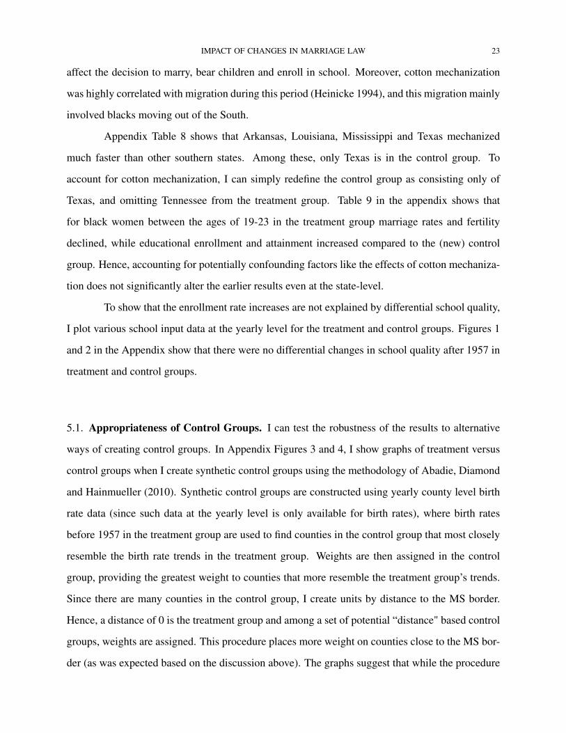
4.2. Fertility. Figure 6 provides some visual evidence that, while there was no relationship be-

tween the change in births between 1950-1954 and distance to the Mississippi border, the largest

drop in number of births per 1000 in the population occur near the border to Mississippi by 1960.

As distance from the border increases, the drop in births appears to decrease. Column 2 in Table 2

shows that counties closer to the border after 1957 had a statistically significant drop in crude birth

rates (the estimation follows equation 1 using the log crude birth rate as the dependent variable).

However, unlike the graphs and figures used to show the decline in marriages, the drop in births

is smaller in magnitude and hence is better represented in regression tables. Figure 6 shows that

areas close to the border after the law change show greater negative changes (this was not the case

before the law change) than areas further away.

16 BHARADWAJ

Table 5 follows a similar estimation strategy as that of Table 3. Equation 1 is estimated

using log of births per 1000 in the population as the dependent variable. Once again, it is clear that

adding controls does not change the coefficients. While Table 3 shows that marriages increased

slightly in the border counties, Table 4 shows that births decreased (Columns 6 and 7). This is not

inconsistent at all as the overall marriages in the border counties did decline - it is just that before

the change in law, all the marriages were being recorded in Mississippi. The coefficients across the

main specifications including Mississippi suggest a drop around 5-6%. This drop in births is quite

substantial considering that between 1910 and 1954, the drop in crude birth rate was around 16%

for the entire country.

Tables 6a and 6b estimate Equation 1 using yearly county level data. I choose to present

this separately and not as my main specification as I do not have data for control variables like

wages and employment at the yearly level. Table 6a uses this yearly data and defines years after

1957 as years affected by the law change. The difference-in-differences coefficient in this table is

negative throughout, even with the inclusion of state and state-by-year fixed effects. The results

also seem robust to the inclusion of state linear and state non-linear time trends (the coefficients of

interest are just shy of significance at the 10% level in the first panel of Table 6a). The middle panel

of 6a estimates the same relationships but restricts the control group to counties within 200 miles

of the Mississippi border. These counties are arguably more similar to Mississippi (see Table 1)

prior to the law change. Again, the results are largely consistent with the top panel. These results

are not affected by the years chosen to be in the sample. In the bottom panel of this table, I restrict

attention to the years 1955-1960 and effects are largely unchanged, suggesting that the effects are

not driven by earlier or later time periods. An important way in which these results differ from the

results in Table 5 is in the magnitude of the coefficients. The coefficients in Table 6a are quite a bit

smaller than those in Table 5. One reason for this is that there were likely changes in 1954-1960

not related to the marriage law change and Table 5 hence might be playing up some of these larger

reasons behind the fertility decline. The estimates in Table 6a suggest a decline in fertility around

2%.


The other major advantage of the yearly data is that I can estimate a difference-in-differences

estimate using each year between 1950-1963 as a placebo year in which the law change occurred.

In other words, I can treat each year as though it were a “treated" year and compute the difference-

in-differences estimates. Hence, if events in 1956 Mississippi unrelated to the law change were

driving the fertility results, we should see the difference-in-differences coefficient for that year

be negative and significant. Table 6b shows that it is precisely in 1958 that the difference-in-

differences coefficient becomes negative and statistically significant.13 In years prior to 1958, the

difference-in-differences coefficient is positive (although not statistically significant), indicating

that the treated counties had a higher birth rate compared to the control counties, and this begins to

change precisely in 1958. However, as is clear from the estimates, while consistent with the idea

that the law change is driving these results, the existence of a mild pre-trend (although not statisti-

cally significant) and the lack of a strict trend-break around 1957 in some specifications should be

treated with caution. Accounting for state specific trends does not change the results much, except

that some of the difference-in-differences coefficients are no longer statistically significant.

Another source of yearly data on fertility is the Vital Statistics tabulations of the number

of births at the state-level. One advantage of these tabulations over the yearly county level data is

that these tabulations are available by race and age. Tables 7a and 7b explore the fraction of births

by race and age in a similar difference-in-differences set up as in equation 1. Table 7a shows that

the decline in births is for younger age groups and is larger in magnitude for blacks. Hence, it

corroborates the results presented earlier showing that the law perhaps affected blacks more. The

Vital Statistics also reports the number of illegitimate births by age and race for this time period.

For younger women, I find an increase in illegitimate births after the passage of the law (Table 7b).

Hence, while the law in effect prevented younger age groups from marrying and having children,

it did have some unintended consequences as it raised the number of illegitimate children.

Data from the census reveals that women affected by the law change in Mississippi were

less likely to have children compared to women not affected by the law change. Table 8 shows that

compared to older groups in control counties, black women in the age group 16-20 are nearly 10

13Note that each coefficient shown in this table comes from a separate regression.

18 BHARADWAJ

percentage points less likely to have a child. The fraction of black women in 1950 in this age range

that had children was around 43%. Hence, relative to that mean, this is a large effect. Comparing

the DD coefficient of this age group to the age group 26-30 shows that it was the younger groups

that were most affected. As in the case of marriage rates, blacks appear more affected than whites

and seem to be driving the overall results. This is perhaps another reason why the results in the

overall county level data sets are perhaps a bit muted in comparison. County level data by race

might show sharper decreases.

Taken together, the results from county and state-level data support the idea that increasing

barriers to marriage led to a decrease in birth rates, at least in the immediate short run by the early

1960s. Later in this section, I examine some of the long run consequences on fertility due to the

change in marriage law in Mississippi. However, given the larger declines in fertility that were

taking place all over the country during this period, some of the declines using broader differences

(1954-1960, or 1950-1960) could be capturing more than just the changes due to the law change.

However, the results by distance to the Mississippi border, analysis by age of the mother, and the

results using county level yearly data should mitigate concerns that forces other than the marriage

law are driving all the results.

4.3. School Enrollment. Goldin and Katz (2002) find that when women have control over their

fertility, they invest more in their career. Does a change in marriage law discouraging early mar-

riage have a similar effect? According to Field and Ambrus (2006), a mandated increase in the

minimum age of marriage should result in greater educational attainment for women. Using the

same empirical strategies as before, I examine whether the change in law led to greater educational

attainment and enrollment. Unfortunately, data on school enrollment is not as extensive for this

period as the data on fertility. For example, there are no comparable yearly county or state-level

data on enrollment rates for all treatment and control areas.

The county level data for enrollment only exists for 1950 and 1960 (this is because com-

parable enrollment data was only available via the Historical census). Hence, I cannot produce

a graph similar to Figures 5 and 6 – instead, in Figure 7, I plot the 1960-1950 difference against

distance to Mississippi border. The graph indicates a strong trend similar to Figure 5, in that areas


close to the border experience the highest gains in enrollment. Column 3 in Table 2 shows that

counties closer to the border after 1957 had statistically higher enrollment rate gains compared to

counties further away (the estimations follows equation 1 using enrollment rates as the dependent

variable).

Table 9 shows estimates the DD coefficients for school enrollment. Similar to Tables 3 and

5, I estimate equation 1 using percentage of 14-17 year olds enrolled in school as the dependent

variable. The DD estimates across all specifications are robust to the addition of controls and

suggest that the change in marriage law led to a 2.5 percentage point increase in school enrollment

for this age group. Since overall school enrollment rates were quite high, this represents a small

increase of 3% over the mean enrollment at that time. During the decade of 1950-1960, there were

no changes to compulsory schooling laws in Mississippi or its neighboring states (Dahl 2009).

These findings are in line with Field and Ambrus (2006) who posit that a compulsory increase in

marriage age will lead to greater school attainment. Unfortunately, the county level data does not

permit an analysis of schooling attainment by 1960. This is because schooling attainment data is

only collected for people above the age of 25 who are too old to be affected by the law.

Using data from the census, I show that black enrollment rates for the younger age groups

were the most impacted. Compared to older age groups and to the control states, Table 10 shows

that black men and women between ages 16-20 had higher enrollment rates in 1960. As in the case

of the other outcomes examined, the overall results appear to be driven by the results for blacks.

A concern might be that these results are driven by changes in the quality of education during

this period in treatment compared to control groups. In Appendix Figures 1 and 2, I show that

treatment groups did not have a differential change in conventional school quality measures during

this time period. Moreover, Appendix Table 7a shows that employment and wages did not change

differentially in treatment areas during this time period, thus making it unlikely that changes in

returns to education explain the increase in enrollment rates (I explain Appendix Table 7a in detail

in the section on robustness checks).

4.4. Evidence from law changes in other states. In 1957 a few other states, (not those in our

treatment or control group) also instituted changes in their marriage laws. These changes, however,

20 BHARADWAJ

did not alter the minimum age of marriage, but instead increased premarital requirements as in the

case of South Carolina, where a parental affidavit was required for parties under the age of 16.

Other states more broadly instituted requirements for blood tests (some of these were repealed in

the 1980s as discussed in Buckles, Guldi and Price (2011)). The states that experienced a change

in law around the same time period were Arizona, New Mexico, Iowa, Indiana and South Carolina

(Plateris 1966).14 Using the same strategy as in equation 2 and using census data, we can examine

whether these changes in law resulted in decreases in marriage rates and fertility.

Table 11 suggests that marriage laws had little impact in Arizona, New-Mexico (I combine

these states into one treatment group since they share a border) and Indiana on the probability

of marriage for different age groups. However, in Iowa there does appear to be a sizable effect

concentrated in the early age groups, just as in Mississippi. However, Mississippi had an equally

sizable negative effect for the next age category as well (this coefficient is just shy of significance

at the 10% level). Note that the results for Mississippi are different in this table as I use a more

restricted version of treatment and control (Mississippi is treatment and neighboring states are

control). This is to make it compatible with the other states examined where I use just the state as

the treated area and its neighbors as the control. Comparing the results of other states to that of

Mississippi shows that the law changes in Mississippi had a much bigger impact than elsewhere.

This is likely due to the age and other restrictions included in the new Mississippi law which were

not a feature of the law changes in other states that focused mainly on blood tests. It is also likely

that since blacks were more impacted by the law change (blood tests and other requirements were

likely more expensive for blacks), and blacks comprised a significant fraction of the population in

Mississippi, that we see larger effects in Mississippi.

4.5. Long run outcomes. Using the census of 1970 and 1990, I examine the long run impacts

of the law change. I do this by using age in 1957 as a variable that defines treatment, along

14It is difficult to pin down precisely what the changes in law in these other states were. Examining law citations fromWestLaw and LexusNexus, it appears that the change in law in Arizona, New Mexico and Indiana was a change inblood test requirement, while the change in South Carolina was a change in parental consent. I was not able to find asimilar citation for the Iowa law change.


with residence in Mississippi and neighboring states. For example, I consider a 17-year-old liv-

ing in Mississippi in 1957 as treated and a 30-year-old in Mississippi in 1957 as untreated. The

difference-in-differences comes from using other states in southern US as my control states. More-

over, I examine all long run outcomes only for black females since they are the most affected group.

The short run effects for whites are quite muted, so the long effects are equally negligible.

Appendix Table 5 shows that people affected by the law in the relevant states had by 1970

a higher age at marriage and fewer children. However, there is no impact on the probability of

marriage or the probability of having a child. Hence, these results are very consistent with the

notion that marriage laws affect the timing of marriage and fertility, but not the extensive margin

of these decisions themselves. There appears to be a positive effect on high school completion,

although this effect is not significant. Panel B of Appendix Table 5 conducts a placebo test to

ensure that the long run results are not picking some inherent trend in reporting by 1970. Using

age groups that were not affected by law, I find no evidence of similar results for the placebo group.

Indeed, the few results that are significant, go in the opposite direction.

In Appendix Table 6 I use the 1990 census to examine whether the results seen in 1970

still persist. This table reveals that by 1990, the difference in number of children born disappears,

suggesting that the fertility effects seen in earlier censuses are largely the effects of timing. As one

might expect, however, the education results appear to be persistent. The analysis of the 1970 and

1990 census suggest that the Mississippi marriage law change largely had an impact of delaying

marriage and fertility. However, it does appear to have had a lasting impact on years of schooling.

5. ROBUSTNESS CHECKS

If there are differential trends in treatment and control groups along any outcome that

could be related to marriage, fertility and schooling, then the results in the previous sections could

be driven by those trends rather than the change in marriage law. In this section, I explore var-

ious labor market and technology related outcomes for the treatment and control groups. In his

analysis of black teenage employment in the South between 1950-1970, Cogan (1981) posits that

"technological progress is the principal cause of the agricultural employment decline among black

22 BHARADWAJ

youth". Hence, we might worry that the treatment and control counties have differential trends in

the adoption or use of various agricultural technologies leading to differential trends in marriage,

fertility and schooling.

Appendix Table 7a shows a DD estimate for various labor market and technological out-

comes. Manufacturing employment, manufacturing wage, and tractor use on farms do not seem

to have changed differentially in treatment counties after the passage of the marriage law. How-

ever, the number of farms per 1000 in the population as well as agricultural employment seem to

have differentially decreased after the passage the of the law. Including these variables directly in

regressions in Tables 3, 5 and 9 does not change the DD estimate. Moreover, percent employed

in agriculture seems to have no statistically significant effect on marriages or the crude birth rate

(Column 5 in Tables 3 and 5). Farms per 1000 in the population do not have a statistically sig-

nificant effect on marriages (Column 6, Table 3). Moreover including a state-by-year fixed effect

seems to negate any effect farms per 1000 might have on school enrollment (Column 7, Table 9).

However, to examine this further, I add to the set of controls in Column 5 in Tables 3, 5 and 9

the interactions of farms per 1000 with the Post and Treat dummy. The idea behind this is that

if farms per 1000 before and after the change in law was the real mover in marriage, fertility and

enrollment, including the interaction of farms per 1000 and the Post dummy should capture the

entire treatment effect. Adding these controls makes no differences to the original DD estimates

(results not reported, available upon request).

In Appendix Table 7b, I randomly assign treatment status to counties within the states of

Louisiana, Arkansas, Mississippi, Tennessee and Alabama. With a 1000 repetitions of regressions

of the form of equation 1, I am able to reject that random assignment of treatment can generate the

results obtained by the DD estimate.

A concern I was able to account for effectively in the county level analysis was that of

technological advancement in agriculture in the treatment versus the control group. States like

Mississippi, its neighboring states and Texas (one of the states in the control group) mechanized

much more rapidly than other Southern states. It is important to control for cotton mechanization

because the advent of mechanization could have impacted returns to schooling, which in turn might


affect the decision to marry, bear children and enroll in school. Moreover, cotton mechanization

was highly correlated with migration during this period (Heinicke 1994), and this migration mainly

involved blacks moving out of the South.

Appendix Table 8 shows that Arkansas, Louisiana, Mississippi and Texas mechanized

much faster than other southern states. Among these, only Texas is in the control group. To

account for cotton mechanization, I can simply redefine the control group as consisting only of

Texas, and omitting Tennessee from the treatment group. Table 9 in the appendix shows that

for black women between the ages of 19-23 in the treatment group marriage rates and fertility

declined, while educational enrollment and attainment increased compared to the (new) control

group. Hence, accounting for potentially confounding factors like the effects of cotton mechaniza-

tion does not significantly alter the earlier results even at the state-level.

To show that the enrollment rate increases are not explained by differential school quality,

I plot various school input data at the yearly level for the treatment and control groups. Figures 1

and 2 in the Appendix show that there were no differential changes in school quality after 1957 in

treatment and control groups.

5.1. Appropriateness of Control Groups. I can test the robustness of the results to alternative

ways of creating control groups. In Appendix Figures 3 and 4, I show graphs of treatment versus

control groups when I create synthetic control groups using the methodology of Abadie, Diamond

and Hainmueller (2010). Synthetic control groups are constructed using yearly county level birth

rate data (since such data at the yearly level is only available for birth rates), where birth rates

before 1957 in the treatment group are used to find counties in the control group that most closely

resemble the birth rate trends in the treatment group. Weights are then assigned in the control

group, providing the greatest weight to counties that more resemble the treatment group’s trends.

Since there are many counties in the control group, I create units by distance to the MS border.

Hence, a distance of 0 is the treatment group and among a set of potential “distance" based control

groups, weights are assigned. This procedure places more weight on counties close to the MS bor-

der (as was expected based on the discussion above). The graphs suggest that while the procedure

24 BHARADWAJ

matches quite well on pre-law change trends, the trends after the law change diverge, suggesting a

drop in birth rates in treatment relative to control groups.

Another way to construct control groups is to use propensity matching techniques to place

weights on counties in the control group that match the counties in the treatment group on observ-

ables. For this procedure, we use the data from the City and County Handbook to match on a large

set of observables like marriage rates, birth rates, percent farms, percent employed in manufac-

turing and agriculture, and the manufacturing wage from 1950 and 1954. As Appendix Table 11

suggests, when weighted using the inverse propensity weights, while birth and marriage rates are

not statistically different pre-1960, they are statistically different in 1960. Hence, even with a more

flexible way of constructing control groups, the essence of the results are retained.

6. CONCLUSIONS

This paper shows that raising the cost of marriage can have large impacts on marriage

rates, crude birth rates and school enrollment. Hence, barriers to marriage for women can result in

delayed fertility, and if early marriage can be delayed, can even lead to higher school enrollment.

The change in marriage law in Mississippi in 1957-58 involved an increase in the minimum age of

marriage, parental consent requirements, and other restrictions like blood tests, proof of age and a

compulsory waiting period. Most of the effects appear concentrated on young women as the law

was aimed at preventing marriage and delaying childbearing at a young age. However, I do find a

small increase in illegitimacy after the law was passed. School enrollment rates experienced a small

increase as a result of the law. As Field and Ambrus (2006) suggest, an increase in minimum age

could be one way of creating barriers that could be beneficial for women’s educational outcomes.

However, in large part the law change had bite in this context because the US has good

legal enforcement, unlike other settings, in particular developing countries where knowledge of

such law changes is scarce. For example, in India the minimum marriage age for women is 18

years, yet in a survey of nearly 90,000 married women conducted in 1992-1993, only 35% were

aware of the law. However, in such societies pre-marital sex and child bearing out of wedlock

is rather taboo, so postponing marriage would likely delay fertility and raise schooling. Hence,


with better enforcement of laws, it is likely that even in the developing country context changes in

marriage law would have similar effects to what I find in the case of Mississippi.

This paper contributes to the understanding of how public policy on marriages can affect

important outcomes like fertility and education. While co-habitation rates and out of wedlock

births have been on the rise, marriage still occupies a central role in American society. However,

further research is needed to analyze why raising the cost of marriage (apart from minimum age

laws) can alter the decision to marry. If people take into account the lifetime benefit of marriage

into their decision to marry today, a small increase in costs via, say, proof of age requirement

should not substantially alter this decision. Moreover, such costs should have a smaller effect if

people expect to pay this cost later.

26 BHARADWAJ

7. REFERENCES

Angrist, J & Evans, W. Schooling and Labor Market Consequences of the 1970 State

Abortion Reforms, NBER Working Paper, 1996.

Bauman, LJ & Stein, REK. Psychological Issues in Contemporary Family and Community

Life in Rudolph’s Pediatrics, 2002.

Bertran, M., Duflo, E., & Mullainathan, S. How much should we trust difference-in-

differences estimates?, Quarterly Journal of Economics, 2004.

Blank, R.M., Charles, K.K., Sallee, J.M. A Cautionary Tale about the Use of Administra-

tive Data: Evidence from Age of Marriage Laws, American Economic Journal: Applied Econom-

ics, 1(2): 128Ð49, 2009.

Buckles, K., Guldi, M., Price, J. Changing the Price of Marriage: Evidence from Blood

Test Requirements, NBER Working Paper 15161, 2009.

Cott, N. Public Vows: A History of Marriage and the Nation, Harvard University Press,

2002.

Card, D & Krueger, A. School Quality and Black-White Relative Earnings: A Direct As-

sessment, Quarterly Journal of Economics, 1992.

Dahl, G. Early Teen Marriage and Future Poverty, forthcoming in Demography, 2009.

Field, E & Ambrus, A. Early Marriage, Age of Menarche and Female Schooling Attain-

ment in Bangladesh, Journal of Political Economy, 2008.

General Laws of the State of Mississippi, 1957

Goldin, C & Katz, L. The Power of the Pill: Oral Contraceptives and Women’s Career

and Marriage Decisions, Journal of Political Economy, August 2002.

Heckman, J & McCurdy, T. A Dynamic Model of Female Labor Supply, Review of Eco-

nomic Studies, 1980.

Heinicke, C. African-American Migration and Mechanized Cotton Harvesting, 1950-1960,

Explorations in Economic History, 1994.

Mississippi Statistical Abstract, 1973. Division of Research, College of Business and

Industry, Mississippi State University.


Plateris,A. The Impact of the Amendment of Marriage Laws in Mississippi, Journal of

Marriage and the Family, 1966.

Raley, RK. Increasing Fertility in Cohabiting Unions - Evidence for the Second Demo-

graphic Transition in the United States?, Demography, 2001.

Rasul, I. Marriage Markets and Divorce Laws, Journal of Law, Economics, and Organi-

zation, 2006.

Stevenson, B. & Wolfers, J. Bargaining in the Shadow of the Law: Divorce Laws and

Family Distress, Quarterly Journal of Economics, 2006.

Stevenson, B. Impact of Divorce Laws on Marriage Specific Capital, Journal of Labor

Economics, 2007.

Stevenson, B. Divorce Laws and Women’s Labor Supply, Journal of Empirical Legal Stud-

ies, 2008.

Vital Statistics of Mississippi, various years. Obtained parts of these publications via

personal contact with Mississippi Department of Public Health.

28 BHARADWAJ

8. ONLINE DATA APPENDIX - NOT FOR PUBLICATION

8.1. County level data. The city and county data book from years 1948, 1950, 1954 and 1960

were used ( County and City Data Book Consolidated Data File 1947-1977). The paper uses the

following variables:

• Marriages: Number of marriages, 1948, 1950, 1954 & 1960

• Births: Total number of births - 1948, 1950, 1954 & 1960 (starting in 1964 this changes to

number of live births)

• Population: Total population for 1950 & 1960

• Farms: Number of farms 1950, 1954 & 1960

• Manufacturing wages: Data available for 1947, 1954 & 1958. I use the 1947 data as proxy

for 1950 data, and 1958 data as proxy for 1960 data for this variable. This variable is in

1000’s of dollars.

• Percent farms with tractors: Data available for 1954 and 1959. I use the 1959 data as proxy

for 1960 data.

• Employment in agriculture: total employment in agriculture, data available for 1950 and

1960

• Manufacturing employment: total employed in manufacturing. Data available for 1949,

1950, 1954 & 1958. 1949 data proxies for 1948 data, and 1958 data proxies for 1960 data.

8.2. Historical Census. The historical census of 1950 and 1960 was used to construct the enroll-

ment variables at the county level.

• Population: Population between the ages of 14-17. This variable was needed from the 1960

census

• Enrollment: Population enrolled between the ages of 14-17, also collected from the 1960

cenus.

• Percent enrolled: Percent 14-17 year olds enrolled. This variable was directly obtained

from the 1950 census.


8.3. Census Variables. 1% sample from the 1950 and 1960 censuses were used. The paper uses

the following variables:

• STATEFIP: reports the state in which the household was located.

• MARST: gives each person’s current marital status. For the 1950 and 1960 census, this

was asked of women above the age of 14.

• SEX: reports whether the person was male or female.

• RACE: the detailed version of this variable was used.

• AGE: reports the person’s age in years as of the last birthday.

• PERWT: indicates how many persons in the U.S. population are represented by a given

person in an IPUMS sample. PERWT must be used to get representative statistics from the

1950 census.

• SCHOOL: indicates whether the respondent attended school during a specified period. This

variable is used to construct the school enrollment variable used in the paper. For the 1950

and 1960 censuses, if a person attended school 2 months prior to the census on April 1st of

that year, they were coded as attending schooling. In the 1950 census, this question is only

asked of Sample Line Individuals. Hence, appropriate weights have to be used while using

this variable from 1950.

• HIGRADE: reports the highest grade of school attended or completed by the respondent.

Again in 1950, this variable is only available for Sample Line Individuals.

• NCHILD: counts the number of own children (of any age or marital status) residing with

each individual. NCHILD includes step-children and adopted children as well as biological

children.

• SLWT: reports the number of persons in the general population represented by each sample-

line person in 1940 and 1950. In 1950, SLWT has a value of zero for non-sample-line per-

sons. For years in which there is no sample-line record (like 1960), SLWT is the same as

person weight, PERWT (the number of persons in the population represented by the case).

8.4. Defining Treatment and Control Groups.

30 BHARADWAJ

8.4.1. Definition of border county. Treatment group consists of all counties in Mississippi and

counties bordering Mississippi. The following are counties bordering Mississippi: Chicot, Choctaw,

Colbert, Concordia, Desha, East Carroll, East Feliciana, Fayette, Franklin, Hardeman, Hardin,

Lamar, Lauderdale, Lee, Madison, Marion, Mc Nairy, Mobile, Phillips, Pickens, Shelby, St He-

lena, Sumter, Tangipahoa, Tensas, Washington, West Feliciana

8.4.2. Creating Figures 3 and 4. Data for Figures 3 and 4 are from the County and City Data Book

Consolidated Data File 1947-1977. The maps were created using GPS Visualizer available as of

this writing at www.gpsvisualizer.com.

8.4.3. Treatment group at the state-level. Treatment group at the state-level consists of Missis-

sippi, Alabama, Louisiana, Arkansas and Tennessee. Control group consists of Texas, Florida,

Oklahoma, Virginia, West Virginia, Georgia, Kentucky, North Carolina, Delaware, Maryland and

Washington DC. South Carolina is excluded as it too had a change in marriage law at the same time

(around 1956). However, including South Carolina in the control group does not significantly alter

the results. As can be seen in Figures 3 and 4, there does not appear to have been a vast change in

marriages in SC after the change in marriage law.

Figure 1

Figure 2

Notes: Data from Vital Statisics. Neighboring states of MS are Arkansas, Tennessee, Louisiana and Alabama. Marriage rates are marriages per 1000 in the population.

Notes: Data from Vital Statistics of Mississippi. Figure shows number of marriages (regardless of residence of bride and groom) that occurred in Mississippi.

Figure 3a - Change in Marriages 1950-1954

Figure 3b - Change in Marriages 1954-1960

Notes: Change in marriages is the percent change from the previous year of available data. Absolute value of the percent change is shown on the maps. County level data is from the County and City Databook 1950, 1954 and 1960.

Figure 4a

Figure 4b

Notes: Data for Figure 4a uses the Census of 1930-1970. Data for Figure 4b uses the census of 1960 and 1970 and computes fraction married using data on age of marriage reported.

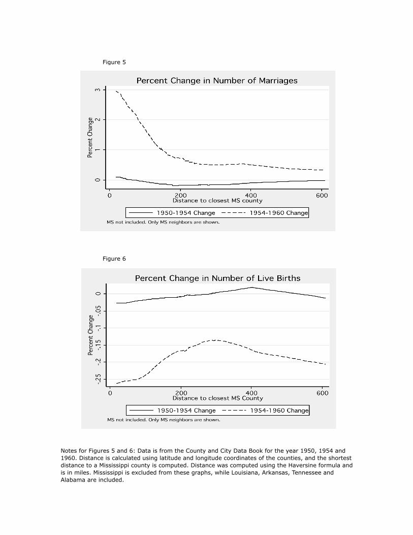
Figure 5

Figure 6

Notes for Figures 5 and 6: Data is from the County and City Data Book for the year 1950, 1954 and 1960. Distance is calculated using latitude and longitude coordinates of the counties, and the shortest distance to a Mississippi county is computed. Distance was computed using the Haversine formula and is in miles. Mississippi is excluded from these graphs, while Louisiana, Arkansas, Tennessee and Alabama are included.

Figure 7

Notes: Data is from the Historical Census of 1950 and 1960 at the county level. Distance is calculated using latitude and longitude coordinates of the counties, and the shortest distance to a Mississippi county is computed. Distance was computed using the Haversine formula and is in miles. Mississippi is excluded from these graphs. Louisiana, Arkansas, Tennessee and Alabama are included. Data for inter censal years is not available.

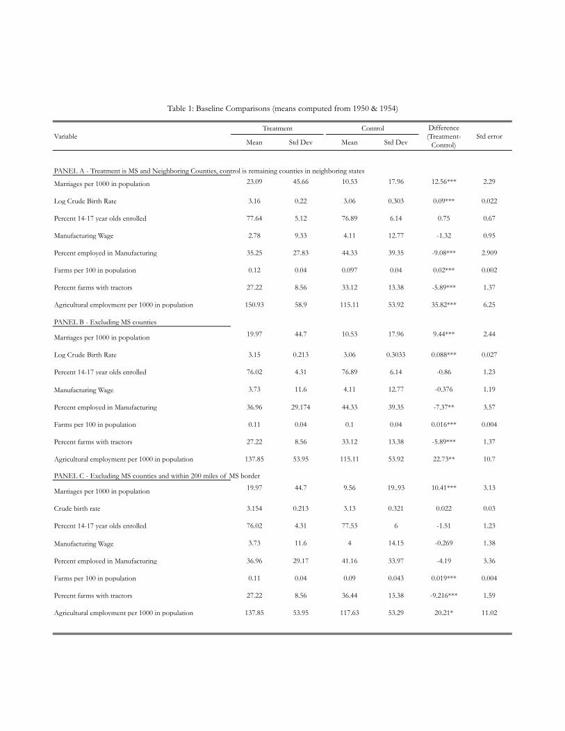
Mean Std Dev Mean Std Dev

PANEL A - Treatment is MS and Neighboring Counties, control is remaining counties in neighboring states

Marriages per 1000 in population 23.09 45.66 10.53 17.96 12.56*** 2.29

Log Crude Birth Rate 3.16 0.22 3.06 0.303 0.09*** 0.022

Percent 14-17 year olds enrolled 77.64 5.12 76.89 6.14 0.75 0.67

Manufacturing Wage 2.78 9.33 4.11 12.77 -1.32 0.95

Percent employed in Manufacturing 35.25 27.83 44.33 39.35 -9.08*** 2.909

Farms per 100 in population 0.12 0.04 0.097 0.04 0.02*** 0.002

Percent farms with tractors 27.22 8.56 33.12 13.38 -5.89*** 1.37

Agricultural employment per 1000 in population 150.93 58.9 115.11 53.92 35.82*** 6.25

PANEL B - Excluding MS counties

Marriages per 1000 in population 19.97 44.7 10.53 17.96 9.44*** 2.44

Log Crude Birth Rate 3.15 0.213 3.06 0.3033 0.088*** 0.027

Percent 14-17 year olds enrolled 76.02 4.31 76.89 6.14 -0.86 1.23

Manufacturing Wage 3.73 11.6 4.11 12.77 -0.376 1.19

Percent employed in Manufacturing 36.96 29.174 44.33 39.35 -7.37** 3.57



Agricultural employment per 1000 in population 137.85 53.95 115.11 53.92 22.73** 10.7

PANEL C - Excluding MS counties and within 200 miles of MS border

Marriages per 1000 in population 19.97 44.7 9.56 19..93 10.41*** 3.13

Crude birth rate 3.154 0.213 3.13 0.321 0.022 0.03

Percent 14-17 year olds enrolled 76.02 4.31 77.53 6 -1.51 1.23

Manufacturing Wage 3.73 11.6 4 14.15 -0.269 1.38

Percent employed in Manufacturing 36.96 29.17 41.16 33.97 -4.19 3.36



Agricultural employment per 1000 in population 137.85 53.95 117.63 53.29 20.21* 11.02

Table 1: Baseline Comparisons (means computed from 1950 & 1954)

VariableTreatment Control Difference

(Treatment-Control)

Std error

Marriages Log CBR Enrollment

1 2 3

Distance Inverse X Post 138.37 -11.19*** 185.8***

[67.162]** (1.587) (42.53)Inverse of distance to MS border -240.53 7.198*** -79.61**

[68.91]*** (1.367) (39.34)Post (=1 if year ≥ 1957) -3.485 -0.233*** 4.698***

[1.645]** (0.0238) (0.563)Fixed Effects used

Controls

Mean of dependent variable 10.02 3.006 80.29R-squared 0.08 0.505 0.427Observations 903 903 586* significant at 10%; ** significant at 5%; *** significant at 1%, robust std errors, clustered at the county level

Table 2: Impact of Marriage law and distance from Mississippi border

State, Year

Manufacturing wage, Farms per 1000 people, Percent employed in Manufacturing

Notes: Marriages are marriages per 1000 in population, births are log births per 1000 in population and enrollment is the percentage of 14-17 year olds enrolled in school. Distance (in miles) is computed using latitude-longitude information on counties and distance to the closest MS county using the Haversine formula is used. Mississippi is excluded from these regressions, as all points within Mississippi have a distance of 0. Counties from neighboring states of MS used .

1 2 3 4 5 6 7

Post X Treatment -12.678 -12.509 -12.509 -13.389 -10.414 4.96 4.303

[3.656]*** [3.749]*** [3.756]*** [4.027]*** [4.077]** [1.241]*** [0.910]***Treatment (=1 if MS or county bordering MS)

11.657 11.626 -1.232 0.628 1.83 -5.6 -5.309

[4.010]*** [4.104]*** [1.319] [1.501] [2.509] [0.808]*** [0.737]***Post (=1 if year ≥ 1957) -0.135 -0.305 -0.026 -2.188 -4.195 -2.662 2.902

[0.451] [0.919] [1.093] [1.451] [1.748]** [1.413]* [0.790]***Manufacturing wage -0.051 -0.042 -0.037 -0.051

[0.039] [0.032] [0.032] [0.033]Farms per 1000 in population 1.186 20.608 11.794 1.978

[21.637] [29.631] [17.796] [17.846]Percent employed in Mfgr 0.047 0.005 0.048 0.044

[0.040] [0.029] [0.043] [0.043]Percent employed in Agri -0.037

[0.034]

Fixed Effects used None None State , Year State , Year State , Year State , Year State X Year

Control Group All counties in Southern USA

Mean of dependent variable 12.04 12.82 12.98

R-squared 0.01 0.04 0.09 0.09 0.08 0.08 0.16Observations 5807 1532 1532 1149 766 903 903

* significant at 10%; ** significant at 5%; *** significant at 1%, robust std errors, clustered at the county level

13.05 10.05

Notes: Cols 1-5 use a state-year cluster, and columns 6 and 7 use a treament group, state -year cluster since MS is excluded in these regressions. Dependent variable is marriages per 1000 of the population. Data from city and county data book for years 1948, 1950, 1954, and 1960 is used. Population at the county level for 1950 and 1960 is used to compute the percentages (1954 numbers are divided by the population in 1950). Treatment is 1 if state is Mississippi and border counties. Percent employed in manufacturing and agriculture also uses population from 1950 and 1960 as the base. Agricultural employment data is only available for 1950 and 1960. Manufacturing employment and wages data is not available for 1948. Regression follows equation 1 in the paper.

Table 3: Impact of Marriage Law on Marriages

Marriages per 1000 in population

All treatment counties used MS not included

----------------------------------Counties in states neighboring MS only----------------------

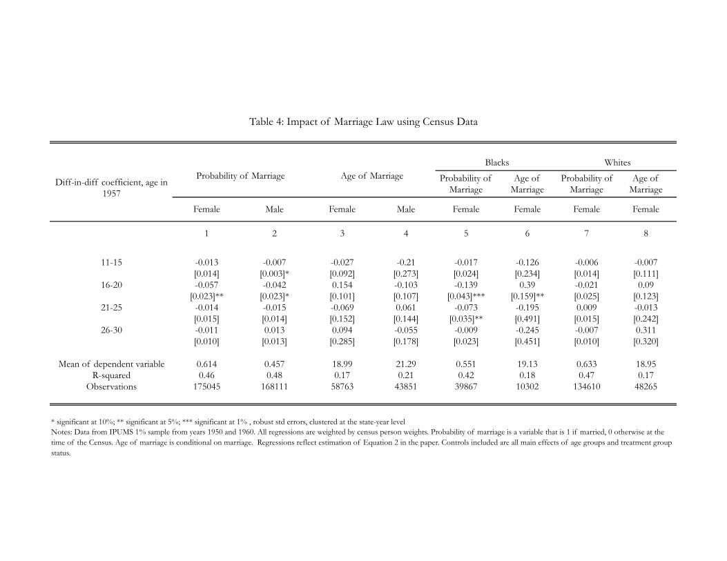
Probability of Marriage

Age of Marriage

Probability of Marriage

Age of Marriage

Female Male Female Male Female Female Female Female

1 2 3 4 5 6 7 8

11-15 -0.013 -0.007 -0.027 -0.21 -0.017 -0.126 -0.006 -0.007[0.014] [0.003]* [0.092] [0.273] [0.024] [0.234] [0.014] [0.111]

16-20 -0.057 -0.042 0.154 -0.103 -0.139 0.39 -0.021 0.09[0.023]** [0.023]* [0.101] [0.107] [0.043]*** [0.159]** [0.025] [0.123]

21-25 -0.014 -0.015 -0.069 0.061 -0.073 -0.195 0.009 -0.013[0.015] [0.014] [0.152] [0.144] [0.035]** [0.491] [0.015] [0.242]

26-30 -0.011 0.013 0.094 -0.055 -0.009 -0.245 -0.007 0.311[0.010] [0.013] [0.285] [0.178] [0.023] [0.451] [0.010] [0.320]

Mean of dependent variable 0.614 0.457 18.99 21.29 0.551 19.13 0.633 18.95R-squared 0.46 0.48 0.17 0.21 0.42 0.18 0.47 0.17

Observations 175045 168111 58763 43851 39867 10302 134610 48265

* significant at 10%; ** significant at 5%; *** significant at 1% , robust std errors, clustered at the state-year levelNotes: Data from IPUMS 1% sample from years 1950 and 1960. All regressions are weighted by census person weights. Probability of marriage is a variable that is 1 if married, 0 otherwise at the time of the Census. Age of marriage is conditional on marriage. Regressions reflect estimation of Equation 2 in the paper. Controls included are all main effects of age groups and treatment group status.

Table 4: Impact of Marriage Law using Census Data

Diff-in-diff coefficient, age in 1957

Probability of Marriage Age of MarriageBlacks Whites

1 2 3 4 5 6 7Post X Treatment -0.0158 -0.0424* -0.0424* -0.0584*** -0.0558** -0.136*** -0.113***

(0.0185) (0.0216) (0.0216) (0.0218) (0.0274) (0.0286) (0.0307)Treatment (=1 if MS or county bordering MS) 0.0781*** 0.0903*** 0.0487 0.0769** 0.0575* 0.104*** 0.0952***

(0.0213) (0.0253) (0.0397) (0.0308) (0.0324) (0.0338) (0.0358)Post (=1 if year ≥ 1957) -0.269*** -0.242*** -0.310*** -0.320*** -0.300*** -0.322*** -0.371***

(0.00609) (0.0126) (0.0144) (0.0168) (0.0185) (0.0182) (0.0221)Manufacturing wage -0.00117** -0.00139*** -0.00142*** -0.00130***

(0.000479) (0.000497) (0.000463) (0.000461)Farms per 1000 in population -3.222*** -4.138*** -3.336*** -3.353***

(0.228) (0.408) (0.277) (0.280)Percent employed in Mfgr -0.000440 -8.80e-06 -0.000470 -0.000599*

(0.000336) (0.000362) (0.000351) (0.000352)Percent employed in Agri 0.000953***

(0.000359)Fixed Effects used None None State , Year State , Year State , Year State , Year State X Year


Observations 4,650 1,372 1,372 1,029 686 810 810R-squared 0.139 0.182 0.371 0.501 0.503 0.514 0.541


Notes: Dependent variable is log births per 1000 of the population. Data from city and county data book for years 1948, 1950, 1954, and 1960 is used. Population at the county level for 1950 and 1960 is used to compute the percentages (1954 numbers are divided by the average population between 1950 and 1960). Treatment is 1 if state is Mississippi and border counties. Agricultural employment data is only available for 1950 and 1960. Manufacturing employment and wages data is not available for 1948. Regressions reflect estimation of Equation 1 in the paper. Outliers in the dependent variable (top and bottom 5% of the counties with changes in birth rates) removed. Including these counties increases the magnitude of the effect to around 8-9% in columns 1-5 and the effects remaining statistically significant. These estimates are presented in Appendix Table 13.

Table 5: Impact of Marriage Law on Crude Birth Rate

Log Births per 1000 in population



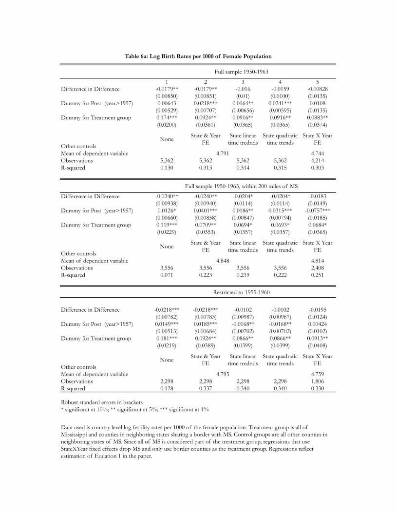
1 2 3 4 5Difference in Difference -0.0179** -0.0179** -0.016 -0.0159 -0.00828

(0.00850) (0.00851) (0.01) (0.0100) (0.0135)Dummy for Post (year>1957) 0.00643 0.0218*** 0.0164** 0.0241*** 0.0108

(0.00529) (0.00707) (0.00656) (0.00595) (0.0135)Dummy for Treatment group 0.174*** 0.0924** 0.0916** 0.0916** 0.0883**

(0.0200) (0.0361) (0.0365) (0.0365) (0.0374)

Other controlsNone State & Year

FEState linear

time tredndsState quadratic

time trendsState X Year

FE

Mean of dependent variable 4.744Observations 5,362 5,362 5,362 5,362 4,214R-squared 0.130 0.313 0.314 0.315 0.303

Difference in Difference -0.0240** -0.0240** -0.0204* -0.0204* -0.0183(0.00938) (0.00940) (0.0114) (0.0114) (0.0149)

Dummy for Post (year>1957) 0.0126* 0.0401*** 0.0186** 0.0315*** -0.0757***(0.00660) (0.00858) (0.00847) (0.00794) (0.0185)

Dummy for Treatment group 0.119*** 0.0709** 0.0694* 0.0693* 0.0684*(0.0229) (0.0353) (0.0357) (0.0357) (0.0365)


FEState linear



FE


Difference in Difference -0.0218*** -0.0218*** -0.0102 -0.0102 -0.0195(0.00782) (0.00783) (0.00987) (0.00987) (0.0124)

Dummy for Post (year>1957) 0.0149*** 0.0185*** -0.0168** -0.0168** 0.00424(0.00513) (0.00684) (0.00702) (0.00702) (0.0102)

Dummy for Treatment group 0.181*** 0.0924** 0.0866** 0.0866** 0.0913**(0.0219) (0.0389) (0.0399) (0.0399) (0.0408)


FEState linear



FE


Robust standard errors in brackets* significant at 10%; ** significant at 5%; *** significant at 1%

Restricted to 1955-1960

4.791

4.795

Data used is country level log fertility rates per 1000 of the female population. Treatment group is all of Mississippi and counties in neighboring states sharing a border with MS. Control groups are all other counties in neighboring states of MS. Since all of MS is considered part of the treatment group, regressions that use StateXYear fixed effects drop MS and only use border counties as the treatment group. Regressions reflect estimation of Equation 1 in the paper.

Table 6a: Log Birth Rates per 1000 of Female Population

Full sample 1950-1963

4.848

Full sample 1950-1963, within 200 miles of MS

Difference in Difference Coefficient

1 2 3 41951 0.000464 0.00188 0.0131 0.00421

(0.0108) (0.0189) (0.0115) (0.0190)1952 -0.00290 -0.0251* -0.000120 -0.0184

(0.00843) (0.0141) (0.00957) (0.0152)1953 0.0179** 0.0134 0.0116 0.0157

(0.00855) (0.0141) (0.00940) (0.0148)1954 0.0140 0.0117 0.0118 0.0128

(0.00849) (0.0135) (0.00869) (0.0142)1955 0.0363*** 0.0251* 0.0414*** 0.0335**

(0.00806) (0.0133) (0.00889) (0.0130)1956 0.0148 0.0108 0.0170 0.0242

(0.00918) (0.0161) (0.0107) (0.0159)1957 -0.00641 -0.0149 -0.0136 -0.0127

(0.00820) (0.0151) (0.00926) (0.0156)1958 -0.0138* -0.0148 -0.0303*** -0.0266**

(0.00797) (0.0132) (0.00817) (0.0125)1959 -0.000617 -0.0207 -0.00680 -0.0274

(0.00916) (0.0189) (0.0102) (0.0201)1960 -0.0114 -0.00649 -0.0167 -0.0121

(0.00954) (0.0130) (0.0103) (0.0139)1961 -0.0141 -0.00436 -0.0175* -0.0124

(0.00891) (0.0149) (0.0103) (0.0158)1962 -0.0123 0.00987 -0.0120 0.00437

(0.0113) (0.0167) (0.0119) (0.0176)1963 -0.0137 0.00594 -0.00534 0.00654

(0.0110) (0.0154) (0.0121) (0.0164)

Controls State, Year FE StateXYear FE State, Year FE StateXYear FE

Observations 5362 4214 3556 2,408Robust standard errors in brackets* significant at 10%; ** significant at 5%; *** significant at 1%

Table 6b: Log Birth Rates per 1000 of Female Population

Full Sample Sample within 200 Miles of MS Border

Notes: Reported coefficients are difference in difference coefficients for each year. Separate regressions are estimated for each coefficient in a specification similar to Equation 1. Treatment and control group definitions are the same as in Table 5. Columns including StateXYear FE's have fewer observations as Mississippi is omitted from those regressions (as all of Mississippi is treated as opposed to just border counties in neighboring states).

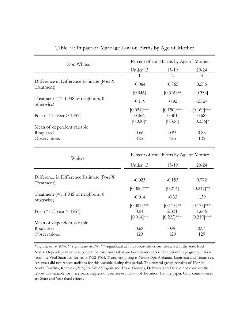
Under 15 15-19 20-241 2 3

Difference in Difference Estimate (Post X Treatment) -0.064 -0.765 0.556

[0.046] [0.316]** [0.334]Treatment (=1 if MS or neighbors, 0 otherwise) -0.119 -0.92 -2.124

[0.024]*** [0.150]*** [0.169]***Post (=1 if year > 1957) 0.066 0.301 -0.683

[0.030]* [0.336] [0.336]*Mean of dependent variableR-squared 0.66 0.83 0.83Observations 125 125 125

Under 15 15-19 20-24

Difference in Difference Estimate (Post X Treatment) -0.023 -0.153 0.772

[0.006]*** [0.214] [0.247]**Treatment (=1 if MS or neighbors, 0 otherwise) -0.014 -0.33 1.39

[0.003]*** [0.115]** [0.133]***Post (=1 if year > 1957) 0.04 2.331 1.646

[0.014]** [0.222]*** [0.219]***Mean of dependent variableR-squared 0.68 0.96 0.94Observations 129 129 129

* significant at 10%; ** significant at 5%; *** significant at 1%, robust std errors, clustered at the state level Notes: Dependent variable is percent of total births that are born to mothers of the relevant age group. Data is from the Vital Statistics, for years 1952-1964. Treatment group is Mississippi, Alabama, Louisiana and Tennessee. Arkansas did not report statistics for this variable during this period. The control group consists of Florida, North Carolina, Kentucky, Virginia, West Virginia and Texas. Georgia, Delaware and DC did not consistently report this variable for these years. Regressions reflect estimation of Equation 1 in the paper. Only controls used are State and Year fixed effects.

Table 7a: Impact of Marriage Law on Births by Age of Mother

Non Whites Percent of total births by Age of Mother

WhitesPercent of total births by Age of Mother

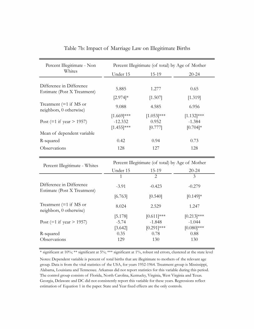
Under 15 15-19 20-24

Difference in Difference Estimate (Post X Treatment) 5.885 1.277 0.65

[2.974]* [1.507] [1.319]Treatment (=1 if MS or neighbors, 0 otherwise)

9.088 4.585 6.956

[1.669]*** [1.053]*** [1.132]***Post (=1 if year > 1957) -12.332 0.952 -1.384

[1.455]*** [0.777] [0.704]*Mean of dependent variable

R-squared 0.42 0.94 0.73

Observations 128 127 128

Under 15 15-19 20-241 2 3

Difference in Difference Estimate (Post X Treatment)

-3.91 -0.423 -0.279

[6.763] [0.540] [0.149]*

Treatment (=1 if MS or neighbors, 0 otherwise)

8.024 2.529 1.247

[5.178] [0.611]*** [0.213]***Post (=1 if year > 1957) -5.74 -1.848 -1.044

[3.642] [0.291]*** [0.080]***R-squared 0.35 0.78 0.88Observations 129 130 130

* significant at 10%; ** significant at 5%; *** significant at 1%, robust std errors, clustered at the state level

Notes: Dependent variable is percent of total births that are illegitimate to mothers of the relevant age group. Data is from the vital statistics of the USA, for years 1952-1964. Treatment group is Mississippi, Alabama, Louisiana and Tennessee. Arkansas did not report statistics for this variable during this period. The control group consists of Florida, North Carolina, Kentucky, Virginia, West Virginia and Texas. Georgia, Delaware and DC did not consistently report this variable for these years. Regressions reflect estimation of Equation 1 in the paper. State and Year fixed effects are the only controls.

Table 7b: Impact of Marriage Law on Illegitimate Births

Percent Illegitimate - Non Whites

Percent Illegitimate (of total) by Age of Mother

Percent Illegitimate - Whites Percent Illegitimate (of total) by Age of Mother

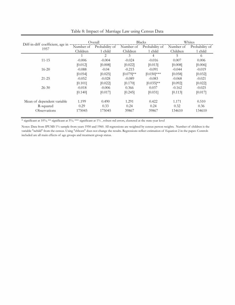
1 2 3 4 5 611-15 -0.006 -0.004 -0.024 -0.016 0.007 0.006

[0.012] [0.008] [0.022] [0.013] [0.008] [0.006]16-20 -0.088 -0.04 -0.215 -0.091 -0.044 -0.019

[0.054] [0.025] [0.079]** [0.030]*** [0.058] [0.032]21-25 -0.052 -0.028 -0.089 -0.083 -0.068 -0.021

[0.101] [0.022] [0.170] [0.035]** [0.092] [0.022]26-30 -0.018 -0.006 0.366 0.037 -0.162 -0.025

[0.140] [0.017] [0.245] [0.031] [0.113] [0.017]

Mean of dependent variable 1.199 0.490 1.291 0.422 1.171 0.510R-squared 0.29 0.33 0.24 0.24 0.32 0.36

Observations 175045 175045 39867 39867 134610 134610

* significant at 10%; ** significant at 5%; *** significant at 1% , robust std errors, clustered at the state-year level

Probability of 1 child

Notes: Data from IPUMS 1% sample from years 1950 and 1960. All regressions are weighted by census person weights. Number of children is the variable "nchild" from the census. Using "chborn" does not change the results. Regressions reflect estimation of Equation 2 in the paper. Controls included are all main effects of age groups and treatment group status.



Overall Blacks WhitesNumber of

ChildrenProbability of

1 childNumber of

ChildrenProbability of

1 childNumber of

Children

1 2 3 4 5 6 7Post X Treatment 2.65 2.658 2.658 2.547 2.244 2.857 2.075

[0.501]*** [0.573]*** [0.575]*** [0.599]*** [0.615]*** [1.121]** [0.943]**Treatment (=1 if MS or county bordering MS)

2.029 0.745 -1.608 -1.34 -0.656 -1.485 -1.073

[0.549]*** [0.620] [0.858]* [0.801]* [0.755] [0.977] [0.933]Post (=1 if year ≥ 1957) 6.725 6.694 6.694 5.985 4.735 5.941 6.825

[0.225]*** [0.357]*** [0.358]*** [0.430]*** [0.450]*** [0.457]*** [0.668]***Manufacturing wage 0.027 0.03 0.03 0.03

[0.013]** [0.014]** [0.014]** [0.015]**Farms per 1000 in population -10.799 30.404 -11.361 -7.806

[7.630] [11.814]** [9.276] [9.340]Percent employed in Mfgr 0.024 0.011 0.026 0.031

[0.008]*** [0.007] [0.009]*** [0.009]***Percent employed in Agri -0.049

[0.010]***

Fixed Effects used None None State , Year State , Year State , Year State , Year State X Year


Mean of dependent variable 79.04

R-squared 0.2 0.31 0.42 0.45 0.48 0.42 0.45Observations 2476 750 750 750 750 586 586


80.85 80.3

Notes: Dependent variable is percent of 14-17 year olds who are currently enrolled in school. Data from the historical census of 1950 and 1960 is used. Treatment is 1 if state is Mississippi and border counties. Percent employed in manufacturing and agriculture uses population from 1950 and 1960 as the base. Agricultural employment data is only available for 1950 and 1960. Regressions reflect estimation of Equation 1 in the paper.

Table 9: Impact of Marriage Law on School Enrollment

Percent of 14-17 year olds enrolled in school



Enrollment Highest grade completed Enrollment Highest grade

completed

Female Male Female Male Female Female Female Female1 2 3 4 5 6 7 8

11-15 0.022 -0.01 0.219 0.242 0.019 -0.116 0.02 0.274[0.023] [0.029] [0.166] [0.171] [0.048] [0.290] [0.026] [0.165]

16-20 0.043 -0.004 0.388 0.327 0.097 0.053 0.024 0.397[0.015]*** [0.026] [0.184]** [0.344] [0.037]** [0.360] [0.021] [0.255]

21-25 0.012 0.019 -0.027 0.248 0.011 -0.004 0.011 0.006[0.010] [0.013] [0.194] [0.268] [0.016] [0.495] [0.013] [0.248]

26-30 -0.008 -0.013 -0.093 0.008 0.005 -0.499 -0.013 0.14[0.016] [0.033] [0.194] [0.223] [0.031] [0.521] [0.016] [0.274]

Mean of dependent variable 0.271 0.326 7.176 7.119 0.287 5.785 0.266 7.589R-squared 0.49 0.39 0.49 0.46 0.46 0.53 0.5 0.48Observations 92666 90218 175045 168111 18552 39867 73796 134610


Notes: Data from IPUMS 1% sample from years 1950 and 1960. All regressions are weighted by census person weights. Regressions reflect estimation of Equation 2 in the paper. Controls included are all main effects of age groups and treatment group status.



Overall Blacks Whites

Enrollment Highest grade completed

Mississippi Arizona & New Mexico

Indiana South Carolina Iowa

1 2 3 4 5

11-15 -0.0362** 0.00273 -0.0106 0.00733 -0.0249*(0.0179) (0.0202) (0.0118) (0.0163) (0.0136)

16-20 -0.0395 -0.0274 -0.0161 -0.0269 -0.0121(0.0262) (0.0274) (0.0199) (0.0267) (0.0261)

21-25 -0.0189 0.0136 0.0330*** 0.00647 -0.0190(0.0184) (0.0189) (0.0122) (0.0184) (0.0160)

26-30 -0.00322 -0.0208 -0.0260*** 0.0131 -0.0121(0.0141) (0.0151) (0.00937) (0.0164) (0.0136)

Mean of dependent variable 0.604 0.649 0.611 0.591 0.600Observations 49,517 83,779 104,196 39,553 65,760




Probability of Marriage: Women

Notes: Data from IPUMS 1% sample from years 1950 and 1960. Regressions represent estimation of equation 2 in the paper. For each state in the columns, the neighboring states are used as a control group. Please see Appendix for list of control states used for each treated state. Controls included are all main effects of age groups and treatment group status.

Documents

IMPACT OF CHANGES IN MARRIAGE LAW: IMPLICATIONS FOR FERTILITY AND SCHOOL … · 2014-08-16 · IMPACT OF CHANGES IN MARRIAGE LAW: IMPLICATIONS FOR FERTILITY AND SCHOOL ENROLLMENT