Embed Size (px)
Citation preview
Impact of Acknowledgments on Application Performance in 4GLTE Networks
by
Brett M. Levasseur
Thesis
Submitted to the Faculty
of the
WORCESTER POLYTECHNIC INSTITUTE
In partial fulfillment of the requirements for the
Degree of Master of Science
in
Computer Science
by
May 2014
APPROVED:
Professor Mark Claypool, Thesis Advisor
Professor Robert Kinicki, Thesis Advisor
Professor Emmanuel Agu, Thesis Reader
Professor Craig E. Wills, Head of Department
i

This work is sponsored by the Department of the Air Force under Air Force Contract
FA8721-05-C-0002. Opinions, interpretations, conclusions and recommendations are those
of the author and not necessarily endorsed by the United States Government.
ii
Abstract
4G LTE is a new cellular phone network standard to provide both the capacity and
Quality of Service (QoS) needed to support multimedia applications. Recent research
in LTE has explored modifications to the current QoS setup, creating MAC layer
schedulers and modifying the current QoS architecture. However, what has not been
fully explored are the effects of LTE retransmission choices and capabilities on QoS.
This thesis examines the impact of using acknowledgments to recover lost data over
the wireless interface on VoIP, FTP and MPEG video applications. Issues explored
include interaction between application performance, network transport protocols, LTE
acknowledgment mode, and wireless conditions.
Simulations show that LTE retransmissions improve FTP throughput by 0.1 to
0.8 Mb/s. With delay sensitive applications, like VoIP and video, the benefits of
retransmissions are dependent on the loss rate. When the wireless loss rate is less than
20%, VoIP has similar performance with and without LTE retransmissions. At higher
loss rates the use of LTE retransmissions adds degrading the VoIP quality by 71%.
With UDP video, the choice of retransmissions or not makes little change when the
wireless loss rates are less than 10%. With higher wireless loss rates, the frame arrival
delay increases by up to 539% with LTE retransmissions, but the frame rate of the
video decreases by up to 34% without those retransmissions.
LTE providers should configure their networks to use retransmission policies appro-
priate for the type of application traffic. This thesis shows that VoIP, FTP and video
require different configurations in the LTE network layers.
iii
Contents
1 Introduction 1
2 Background 4
2.1 Overview of 4G LTE . . . . . . . . . . . . . . . . . . . . . . . . . . . . . . . 4
2.1.1 Network Layers . . . . . . . . . . . . . . . . . . . . . . . . . . . . . . 5
2.1.2 Quality of Service . . . . . . . . . . . . . . . . . . . . . . . . . . . . . 17
2.1.3 Long Term Evolution (LTE) Retransmissions and Applications . . . . 18
2.2 ns-3 . . . . . . . . . . . . . . . . . . . . . . . . . . . . . . . . . . . . . . . . 24
2.2.1 Transmission Control Protocol (TCP) . . . . . . . . . . . . . . . . . . 25
2.2.2 User Datagram Protocol (UDP) . . . . . . . . . . . . . . . . . . . . . 26
2.3 Applications . . . . . . . . . . . . . . . . . . . . . . . . . . . . . . . . . . . . 26
2.3.1 Voice over IP (VoIP) . . . . . . . . . . . . . . . . . . . . . . . . . . . 26
2.3.2 file transfer protocol (FTP) . . . . . . . . . . . . . . . . . . . . . . . 28
2.3.3 Video . . . . . . . . . . . . . . . . . . . . . . . . . . . . . . . . . . . 29
3 Related Work 31
3.1 Applications in Cellular Networks . . . . . . . . . . . . . . . . . . . . . . . . 31
3.2 LTE Measurements . . . . . . . . . . . . . . . . . . . . . . . . . . . . . . . . 32
3.3 hybrid automatic repeat request (HARQ) . . . . . . . . . . . . . . . . . . . . 33
3.4 Radio Link Control (RLC) . . . . . . . . . . . . . . . . . . . . . . . . . . . . 34
3.5 VoIP in LTE . . . . . . . . . . . . . . . . . . . . . . . . . . . . . . . . . . . . 35
4 Approach 36
4.1 Problem Statement . . . . . . . . . . . . . . . . . . . . . . . . . . . . . . . . 36
4.2 Simulator Additions . . . . . . . . . . . . . . . . . . . . . . . . . . . . . . . 39
4.3 Simulator Settings . . . . . . . . . . . . . . . . . . . . . . . . . . . . . . . . 43
iv

4.3.1 VoIP . . . . . . . . . . . . . . . . . . . . . . . . . . . . . . . . . . . . 43
4.3.2 FTP . . . . . . . . . . . . . . . . . . . . . . . . . . . . . . . . . . . . 44
4.3.3 Video . . . . . . . . . . . . . . . . . . . . . . . . . . . . . . . . . . . 45
4.3.4 Simulated Network . . . . . . . . . . . . . . . . . . . . . . . . . . . . 46
4.3.5 Constant Settings . . . . . . . . . . . . . . . . . . . . . . . . . . . . . 46
4.3.6 Variable Settings . . . . . . . . . . . . . . . . . . . . . . . . . . . . . 51
4.3.7 Simulation Time . . . . . . . . . . . . . . . . . . . . . . . . . . . . . 55
5 Results 60
5.1 ns-3 LTE Additions . . . . . . . . . . . . . . . . . . . . . . . . . . . . . . . . 60
5.1.1 Adding NACKs to Status PDUs . . . . . . . . . . . . . . . . . . . . . 60
5.1.2 Detecting Sequence Numbers to NACK . . . . . . . . . . . . . . . . . 60
5.2 Baseline . . . . . . . . . . . . . . . . . . . . . . . . . . . . . . . . . . . . . . 61
5.2.1 No Loss . . . . . . . . . . . . . . . . . . . . . . . . . . . . . . . . . . 61
5.2.2 Basic Loss . . . . . . . . . . . . . . . . . . . . . . . . . . . . . . . . . 66
5.3 VoIP Simulations . . . . . . . . . . . . . . . . . . . . . . . . . . . . . . . . . 73
5.3.1 VoIP with varied RLC settings . . . . . . . . . . . . . . . . . . . . . 73
5.3.2 VoIP with AM vs UM with varied loss . . . . . . . . . . . . . . . . . 82
5.4 FTP Simulations . . . . . . . . . . . . . . . . . . . . . . . . . . . . . . . . . 87
5.4.1 FTP with varied RLC settings . . . . . . . . . . . . . . . . . . . . . . 87
5.4.2 FTP with AM vs UM with varied loss . . . . . . . . . . . . . . . . . 93
5.5 movie picture experts group (MPEG) Simulations . . . . . . . . . . . . . . . 96
5.5.1 MPEG with varied RLC settings . . . . . . . . . . . . . . . . . . . . 96
5.5.2 MPEG with AM vs UM with varied loss . . . . . . . . . . . . . . . . 101
6 Conclusion 103
7 Future Work 106
v
References 107
A Acronyms 113
B channel quality indicator (CQI) 119
C Additional Figures 122
vi
List of Figures
1 Evolved Packet Core . . . . . . . . . . . . . . . . . . . . . . . . . . . . . . . 4
2 Maximum transport block size. . . . . . . . . . . . . . . . . . . . . . . . . . 8
3 Maximum possible throughput in LTE . . . . . . . . . . . . . . . . . . . . . 9
4 Unacknowledged Mode [2] . . . . . . . . . . . . . . . . . . . . . . . . . . . . 12
5 Acknowledged Mode [2] . . . . . . . . . . . . . . . . . . . . . . . . . . . . . . 13
6 AM Transmission Window [30] . . . . . . . . . . . . . . . . . . . . . . . . . . 14
7 AM Reception Window [30] . . . . . . . . . . . . . . . . . . . . . . . . . . . 15
8 Example RLC SDU Segmentation [1] . . . . . . . . . . . . . . . . . . . . . . 15
9 PDCP PDU [1] . . . . . . . . . . . . . . . . . . . . . . . . . . . . . . . . . . 16
10 SAE Bearer Service Architecture [1] . . . . . . . . . . . . . . . . . . . . . . . 17
11 HARQ retransmissions for downlink traffic. This diagram was modified from
an example in [17]. . . . . . . . . . . . . . . . . . . . . . . . . . . . . . . . . 21
12 Simple example of congestion window growth in TCP. . . . . . . . . . . . . . 25
13 Status protocol data unit (PDU) for RLC AM [2] . . . . . . . . . . . . . . . 39
14 Network used during simulations. . . . . . . . . . . . . . . . . . . . . . . . . 46
15 Default simulation radio map. . . . . . . . . . . . . . . . . . . . . . . . . . . 49
16 Gilbert-Elliot model. Figure based on [24]. . . . . . . . . . . . . . . . . . . . 53
17 Standard deviation for the VoIP packets. . . . . . . . . . . . . . . . . . . . . 56
18 Standard deviation for the MPEG application. . . . . . . . . . . . . . . . . . 57
19 Standard deviation of frame sizes and delay for the MPEG application. . . . 59
20 Validation tests of updates to LTE module . . . . . . . . . . . . . . . . . . . 62
21 Baseline delay for UDP packets. . . . . . . . . . . . . . . . . . . . . . . . . . 64
22 TCP rate seen by the UE using RLC AM and UM. . . . . . . . . . . . . . . 64
23 Baseline video frame delay. . . . . . . . . . . . . . . . . . . . . . . . . . . . . 67
24 Sample of 25% fading trace file. . . . . . . . . . . . . . . . . . . . . . . . . . 68
vii
25 RLC AM and UM performance for VoIP with a 25% loss rate. . . . . . . . . 69
26 RLC AM and UM performance for FTP with a 25% loss rate. . . . . . . . . 71
27 Video frame delay with uniform 25% loss. . . . . . . . . . . . . . . . . . . . 72
28 CDF of loss gap lengths. . . . . . . . . . . . . . . . . . . . . . . . . . . . . . 74
29 VoIP t-Reordering tests. . . . . . . . . . . . . . . . . . . . . . . . . . . . . . 77
30 UDP delay when varying t-Reordering timer. . . . . . . . . . . . . . . . . . . 78
31 VoIP t-StatusProhibit tests. . . . . . . . . . . . . . . . . . . . . . . . . . . . 80
32 Maximum possible STATUS PDUs that can be sent in 1 second. . . . . . . . 81
33 Results for different losses with t-Reordering = 30 ms and t-StatusProhibit =
50 ms, with input model gap lengths up to 30. . . . . . . . . . . . . . . . . . 83
34 Results for different losses with t-Reordering = 30 ms and t-StatusProhibit =
50 ms, with input model gap lengths up to 100. . . . . . . . . . . . . . . . . 84
35 25 and 30% loss VoIP AM tests. . . . . . . . . . . . . . . . . . . . . . . . . . 85
36 CDF of loss gap lengths. . . . . . . . . . . . . . . . . . . . . . . . . . . . . . 87
37 Average FTP throughput for t-Reordering. . . . . . . . . . . . . . . . . . . . 89
38 AM t-StatusProhibit . . . . . . . . . . . . . . . . . . . . . . . . . . . . . . . 92
39 Average FTP throughput for t-StatusProhibit. . . . . . . . . . . . . . . . . . 92
40 Average FTP throughput for t-Reordering = 50 ms and t-StatusProhibit =
75 ms . . . . . . . . . . . . . . . . . . . . . . . . . . . . . . . . . . . . . . . 94
41 CDF of loss gap lengths. . . . . . . . . . . . . . . . . . . . . . . . . . . . . . 96
42 Average delay and frame rates for MPEG with varied t-Reordering. . . . . . 99
43 Average delay and frame rates for MPEG with varied t-StatusProhibit . . . 100
44 Average delay and frame rate for t-Reordering = 30 ms and t-StatusProhibit
= 75 ms. . . . . . . . . . . . . . . . . . . . . . . . . . . . . . . . . . . . . . . 101
45 Map of where CQI measurements were taken. . . . . . . . . . . . . . . . . . 120
46 CQI measurements . . . . . . . . . . . . . . . . . . . . . . . . . . . . . . . . 121
47 Baseline RLC Receive Window with VoIP . . . . . . . . . . . . . . . . . . . 122
viii
48 Baseline FTP RLC Receive Windows. . . . . . . . . . . . . . . . . . . . . . . 123
49 Baseline RLC UM receive window for Video. . . . . . . . . . . . . . . . . . . 123
50 RLC performance for FTP with a uniform 25% loss rate. . . . . . . . . . . . 124
ix
List of Tables
1 CQI Table [4]. . . . . . . . . . . . . . . . . . . . . . . . . . . . . . . . . . . . 6
2 modulation and coding scheme (MCS) Modulation and transport block size
(TBS) Index [4]. . . . . . . . . . . . . . . . . . . . . . . . . . . . . . . . . . . 7
3 Listening Quality Scale with MOS [37] . . . . . . . . . . . . . . . . . . . . . 29
4 MPEG frame trace. . . . . . . . . . . . . . . . . . . . . . . . . . . . . . . . . 45
5 Suggested settings from [5] for some RLC layer timers. . . . . . . . . . . . . 55
6 Verizon core network latencies March 2014 [40] . . . . . . . . . . . . . . . . . 75
7 FTP results AM t-Reordering . . . . . . . . . . . . . . . . . . . . . . . . . . 88
8 FTP results UM t-Reordering . . . . . . . . . . . . . . . . . . . . . . . . . . 89
9 FTP results AM t-StatusProhibit . . . . . . . . . . . . . . . . . . . . . . . . 91
10 FTP results AM multiple loss rates . . . . . . . . . . . . . . . . . . . . . . . 93
11 FTP results UM multiple loss rates . . . . . . . . . . . . . . . . . . . . . . . 94
12 MPEG frames lost with UM . . . . . . . . . . . . . . . . . . . . . . . . . . . 98
13 MPEG frames lost with UM . . . . . . . . . . . . . . . . . . . . . . . . . . . 102
x
1 Introduction
In recent years, mobile technology has increased both in capability and penetration in every-
day use. Cisco reports that over half a billion mobile devices and connections were added in
2013 and 77% of this growth came from smartphones [16]. Global mobile data traffic grew
81% and mobile video traffic took up 53% of all mobile data traffic in 2013. Cisco also found
that 4G connections generated 14.5 times more traffic on average than non 4G connections.
While the total number of 4G connections only account for 2.9% of all mobile connections
they account for 30% of mobile traffic. Cisco predicts that by 2018 4G traffic will account
for half of all mobile traffic. With the growing usage of 4G networks research into LTE and
other 4G protocols is important for businesses and users alike.
A common problem for all networks is managing loss and minimizing the delay of data.
For wireless networks this is especially problematic as the wireless link is constantly shifting
in signal quality based on local interference sources like buildings or other radio wave emitting
objects and mobility of the communicating nodes. All wireless networks need to define how
to handle diverse radio environments while maintaining a good quality for users.
As the noise in a signal seen by a device increases, LTE decreases the amount of bits
sent to improve the chances of the data arriving without error. When data is lost LTE
provides retransmissions at two different network layers to reduce loss. LTE also has multiple
parameters that adjust how retransmissions are managed in the network. However, the exact
settings used by a network are not known to its users or application developers. Further,
the network provider may not know what settings they should use.
The choice of how retransmissions are managed has a large impact on the end user appli-
cations. Some programs require all data sent to be received without error like emails or file
transfers. However other application like VoIP or live video streaming need minimal network
delay and can accept some loss. With the multiple ways LTE can configure retransmissions
it is possible that some network configuration may be beneficial to some types of applications
1

while harmful to others.
In previous research into LTE retransmissions authors have focused on one of two retrans-
mission techniques at the Media Access Control (MAC) and RLC layers in LTE but not both.
Kawser et al. [29] looked at how the maximum number of MAC layer retransmissions do not
always improve the total amount of data lost. Makidis [30] simulated RLC retransmissions
with Web and FTP traffic. While this work shows some impacts of using retransmissions it
does not look at any of the adjustable parameters with the RLC layer. Other research into
LTE retransmissions like Asheralieva et al. [9] looked at VoIP simulations in LTE with and
without MAC layer retransmissions. This work did not look at the impact of the RLC layer
retransmissions.
This work examines how configurations in the RLC layer for retransmission of data lost
in the wireless last hop impact applications like VoIP and video that are delay sensitive and
FTP, which is throughput sensitive. Preferred settings are found through simulations of an
LTE network with varied loss rates on the wireless link. These simulations are supported by
an open source To complete this work new code is added to the LTE simulator to support
the use of negative acknowledgments (NACKs) in acknowledged mode (AM), which is part
of the LTE specification but was not implemented in the simulator.
A built in capability of the simulator sets when the wireless noise is great enough to
lose data. A Gilbert Elliot model is used to define at what time, how long and what radio
frequencies experience enough noise to induce loss. First, experiments use VoIP, FTP and
video applications at 10% wireless loss (a goal according to the LTE specification). These
tests adjust two parameters in LTE, the timers t-Reordering and t-StatusProhibit. The
results indicate what settings are preferred for the applications. Next these parameters are
fixed based on the earlier findings and the amount of wireless loss is adjusted. From these
tests we find if the applications perform better when LTE performs extra retransmissions to
recover lost data or not.
Simulations show that LTE retransmissions improve FTP throughput by 0.1 to 0.8 Mb/s.
2
With delay sensitive applications, like VoIP and video, the benefits of retransmissions are
dependent on the loss rate. When the wireless loss rate is less than 20%, VoIP has similar
performance with and without LTE retransmissions. At higher loss rates the use of LTE
retransmissions adds degrading the VoIP quality by 71%. With UDP video, the choice of
retransmissions or not makes little change when the wireless loss rates are less than 10%.
With higher wireless loss rates, the frame arrival delay increases by up to 539% with LTE
retransmissions, but the frame rate of the video decreases by up to 34% without those
retransmissions.
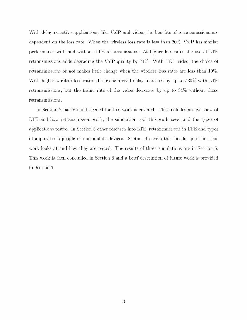
In Section 2 background needed for this work is covered. This includes an overview of
LTE and how retransmission work, the simulation tool this work uses, and the types of
applications tested. In Section 3 other research into LTE, retransmissions in LTE and types
of applications people use on mobile devices. Section 4 covers the specific questions this
work looks at and how they are tested. The results of these simulations are in Section 5.
This work is then concluded in Section 6 and a brief description of future work is provided
in Section 7.
3

Figure 1: Evolved Packet Core
2 Background
2.1 Overview of 4G LTE
Long Term Evolution (LTE) is one of the current 4G cellular phone technologies deployed
in multiple countries around the world. The core network for LTE is known as System Ar-
chitecture Evolution (SAE). This network is split into two primary areas, evolved packet
core (EPC) that makes up the connection from gateways on Internet protocol (IP) networks
to the enhanced node b (eNodeB) access points and evolved universal mobile telecommu-
nications system terrestrial radio access (E-UTRA) that makes up the wireless last link to
user devices known as user equipment (UE) [6]. Unlike previous phone network technologies
like global system for mobile communications (GSM), general packet radio service (GPRS)
and niversal Mobile Telecommunications System (UMTS), LTE is entirely packet switched.
GSM was a circuit switched network while GPRS and UMTS supported both circuit and
packet switching [21]. The LTE network is depicted in Figure 1. The components of the
network are:
• Serving Gateway (SGW) - A node that determines which eNodeB to route and send
packets to.
• Packet Delivery Network Gateway (PGW) - Connectivity to external networks like the
4

Internet.
• enhanced node b (eNodeB) - Wireless access point for the radio interface E-UTRA.
• user equipment (UE) - End devices that connect to the LTE network such as phones,
tablets and computers with LTE connect cards.
2.1.1 Network Layers
In this section we give a brief overview of the layers that make up the wireless link in
LTE. From bottom to top these are the physical, MAC, RLC and Packet Data Convergence
Protocol (PDCP) layers that handle both user data and LTE control messages. Above these
layers LTE has additional control layers called the Radio Resource Control (RRC) and Non
Access Stratum (NAS). The following sections pay particular attention to topics needed for
understanding retransmissions in LTE and size of transmission opportunities.
2.1.1.1 Physical Layer
The physical layer handles transmitting data over radio waves between the eNodeB and
UE. LTE can transmit data in physical resource blocks (PRBs) that take up 0.5 ms slots in
time and 15kHz of radio bandwidth. The more contiguous radio frequencies a LTE network
has the more data can be sent in parallel. The smallest physical resource LTE can send is
a transport block that takes up 1 ms transmission time interval (TTI) (2 slots) and some
number of PRBs depending on what the network has available and what the scheduler allows.
In LTE the maximum number of PRBs in a transport block is 100.
Channel Quality As for other wireless standards, LTE will monitor the quality of the
radio signal and adjust the encoding rate for better performance. A UE will regularly check
the receive signal quality and report a CQIs value (among others values) to the eNodeB. The
CQI represents the data encoding scheme and code rate to use so that the block level error
rate (BLER) of received data is at most 10% [17]. BLER is a major metric in determining
5

Table 1: CQI Table [4].
CQI index Modulation Code Rate x 1024 Efficiency0 out of range1 QPSK 78 0.15232 QPSK 120 0.23443 QPSK 193 0.37704 QPSK 308 0.60165 QPSK 449 0.87706 QPSK 602 1.17587 16QAM 378 1.47668 16QAM 490 1.91419 16QAM 616 2.406310 64QAM 466 2.730511 64QAM 567 3.322312 64QAM 666 3.902313 64QAM 772 4.523414 64QAM 873 5.115215 64QAM 948 5.5547
how to send data in LTE. BLER is specifically defined as the ratio of the number of erroneous
blocks received to the total number of blocks sent where an erroneous block is a transport
block whose cyclic redundancy check is wrong [7]. The modulation determines how many bits
can be encoded per orthogonal frequency-division multiplexing (OFDM) symbol (the method
of encoding bits in the radio spectrum) and the coding rate is the ratio of the number of
bits transmitted compared to the number of bits that could be transmitted. Table 1 shows
CQI values and their meaning.
The eNodeB takes the CQI value and determines a MCSs value between 0 and 31 (though
29 - 31 are reserved for future use). The MCS value selected will not necessarily map to
the same modulation encoding that the UE requested with its CQI. The MCS values and
their modulation (listed in 2, 4 and 6 bits) are shown in Table 2 along with a TBS index.
The TBS index is combined with the number of PRBs to determine how large the transport
block sent is. Possible transport block sizes are given in table 7.1.7.2.1-1 of [4]. For example,
a good signal to noise ratios (SINRs) will have a high MCS value of 28, which maps to a
transport block index of 26. If there are 100 PRBs available then the transport block will be
6
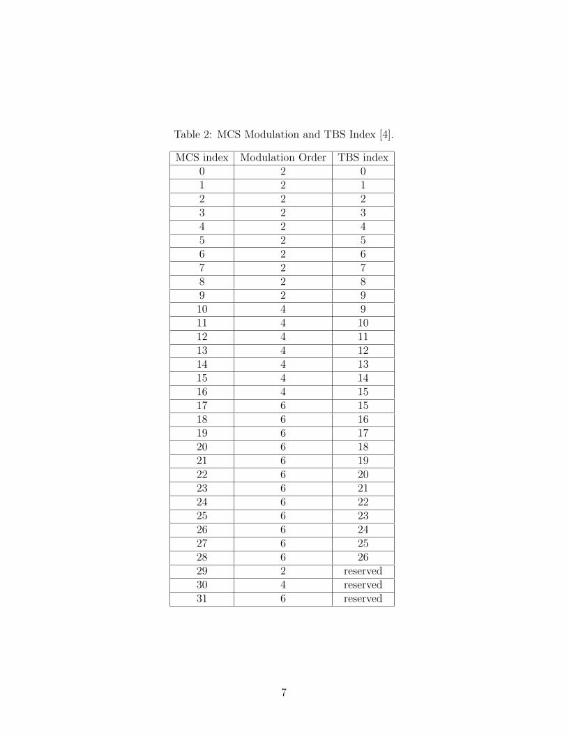
Table 2: MCS Modulation and TBS Index [4].
MCS index Modulation Order TBS index0 2 01 2 12 2 23 2 34 2 45 2 56 2 67 2 78 2 89 2 910 4 911 4 1012 4 1113 4 1214 4 1315 4 1416 4 1517 6 1518 6 1619 6 1720 6 1821 6 1922 6 2023 6 2124 6 2225 6 2326 6 2427 6 2528 6 2629 2 reserved30 4 reserved31 6 reserved
7
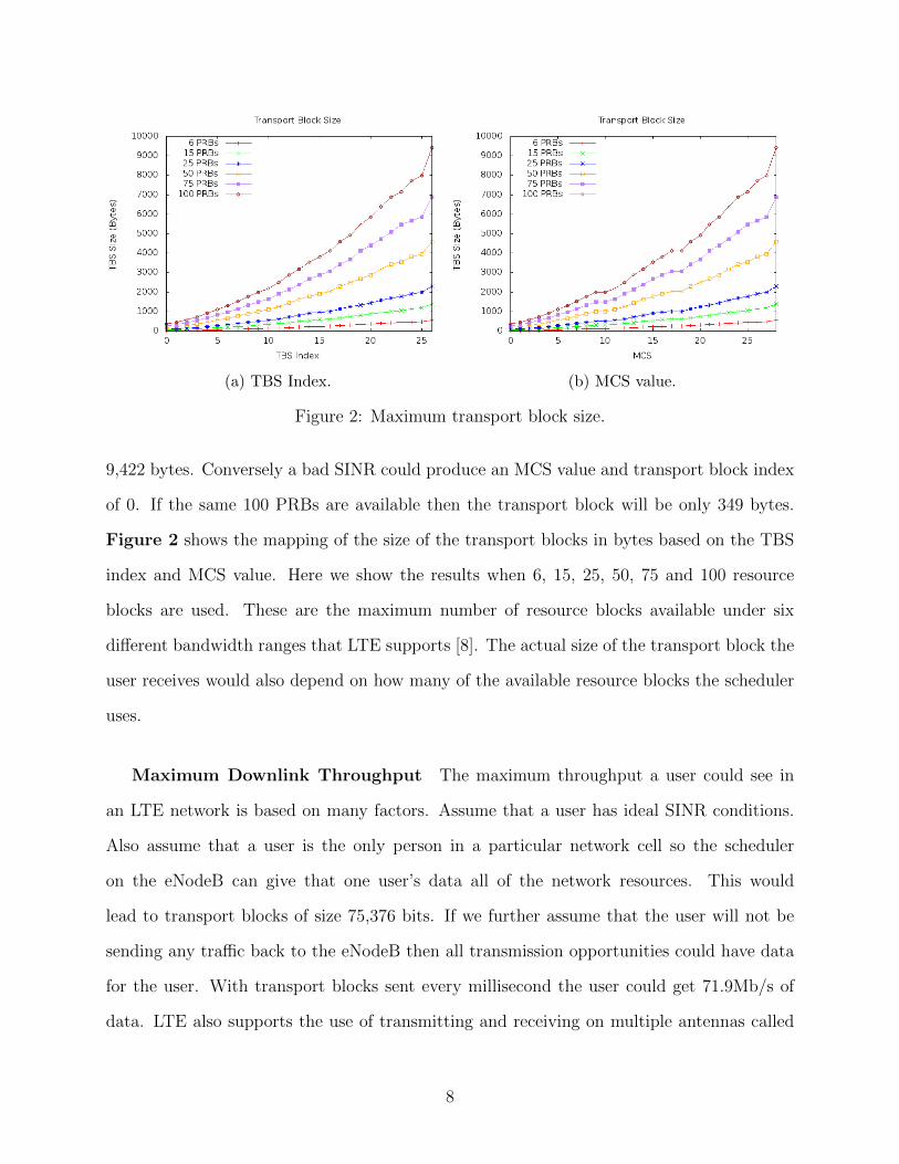
(a) TBS Index. (b) MCS value.
Figure 2: Maximum transport block size.
9,422 bytes. Conversely a bad SINR could produce an MCS value and transport block index
of 0. If the same 100 PRBs are available then the transport block will be only 349 bytes.
Figure 2 shows the mapping of the size of the transport blocks in bytes based on the TBS
index and MCS value. Here we show the results when 6, 15, 25, 50, 75 and 100 resource
blocks are used. These are the maximum number of resource blocks available under six
different bandwidth ranges that LTE supports [8]. The actual size of the transport block the
user receives would also depend on how many of the available resource blocks the scheduler
uses.
Maximum Downlink Throughput The maximum throughput a user could see in
an LTE network is based on many factors. Assume that a user has ideal SINR conditions.
Also assume that a user is the only person in a particular network cell so the scheduler
on the eNodeB can give that one user’s data all of the network resources. This would
lead to transport blocks of size 75,376 bits. If we further assume that the user will not be
sending any traffic back to the eNodeB then all transmission opportunities could have data
for the user. With transport blocks sent every millisecond the user could get 71.9Mb/s of
data. LTE also supports the use of transmitting and receiving on multiple antennas called
8
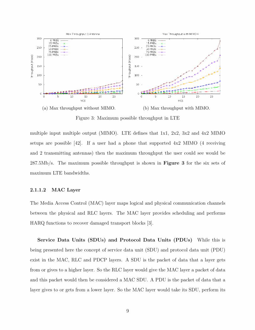
(a) Max throughput without MIMO. (b) Max throughput with MIMO.
Figure 3: Maximum possible throughput in LTE
multiple input multiple output (MIMO). LTE defines that 1x1, 2x2, 3x2 and 4x2 MIMO
setups are possible [42]. If a user had a phone that supported 4x2 MIMO (4 receiving
and 2 transmitting antennas) then the maximum throughput the user could see would be
287.5Mb/s. The maximum possible throughput is shown in Figure 3 for the six sets of
maximum LTE bandwidths.
2.1.1.2 MAC Layer
The Media Access Control (MAC) layer maps logical and physical communication channels
between the physical and RLC layers. The MAC layer provides scheduling and performs
HARQ functions to recover damaged transport blocks [3].
Service Data Units (SDUs) and Protocol Data Units (PDUs) While this is
being presented here the concept of service data unit (SDU) and protocol data unit (PDU)
exist in the MAC, RLC and PDCP layers. A SDU is the packet of data that a layer gets
from or gives to a higher layer. So the RLC layer would give the MAC layer a packet of data
and this packet would then be considered a MAC SDU. A PDU is the packet of data that a
layer gives to or gets from a lower layer. So the MAC layer would take its SDU, perform its
9
processing and then create a MAC layer PDU that it then provides to the physical layer. The
MAC, RLC and PDCP layers will take SDUs from higher layers, perform some processing
to create PDUs to give to lower layers and take PDUs from lower layers, perform some
processing to create SDUs to provide to higher layers. The MAC layer packs only one SDU
per PDU.
Hybrid Automatic Repeat Request (HARQ) The MAC layer’s HARQ process
attempts to correct for any data lost during transmission. For each transport block received
the HARQ mechanism checks to see if the data was received successfully. This is done using
forward error correction (FEC) bits and parity bits that come with the transport block [3].
If no errors are detected then an acknowledgment (ACK) is returned to the sender and the
data is passed up to the higher network layers. If an error is detected then a NACK is
returned and the transport block is kept. On future retransmissions multiple copies of the
damaged data can be combined to create the original data [3]. More information on how
these retransmissions work is in Section 2.1.3.
2.1.1.3 Radio Link Control (RLC) Layer
The Radio Link Control (RLC) Layer provides segmentation and reassembly between the
original data frames and those encoded in the transport blocks [2]. How the RLC layer deals
with segmentation and reassembly depends on the mode of transmission in use. The RLC
layer has several transmission modes, transparent mode (TM) for control data, unacknowl-
edged mode (UM) that just handles out-of-order reassembly and acknowledged mode (AM)
that provides acknowledgments for transport blocks that could not be repaired or retrieved
through the HARQ mechanisms at the MAC layer. While these three modes are different
they all share some features. All modes support a variable size of RLC SDU that must be
a multiple of 8 bits. The data PDUs made in the RLC layer come from RLC SDU handed
down from the PDCP layer. Also all control PDUs are created in the RLC layer itself. All
10
three layers can only transmit PDUs when the lower MAC layer informs of a transmission
opportunity.
transparent mode (TM) TM is used for control messages only and not user applica-
tion data. There is no segmentation or concatenation of RLC SDUs . Unlike in UM and AM
there are no RLC headers added to the PDU. Any PDU received by this layer are delivered
directly to the PDCP layer as there has been no segmentation or reassembly to take into
account.
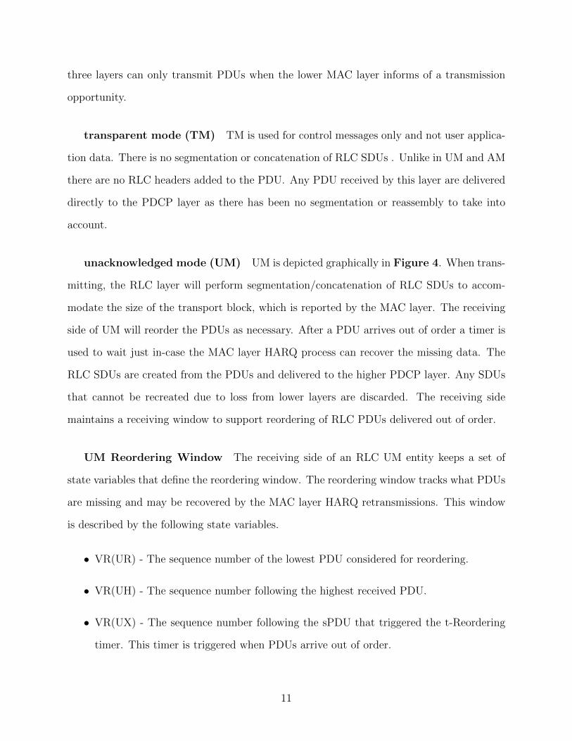
unacknowledged mode (UM) UM is depicted graphically in Figure 4. When trans-
mitting, the RLC layer will perform segmentation/concatenation of RLC SDUs to accom-
modate the size of the transport block, which is reported by the MAC layer. The receiving
side of UM will reorder the PDUs as necessary. After a PDU arrives out of order a timer is
used to wait just in-case the MAC layer HARQ process can recover the missing data. The
RLC SDUs are created from the PDUs and delivered to the higher PDCP layer. Any SDUs
that cannot be recreated due to loss from lower layers are discarded. The receiving side
maintains a receiving window to support reordering of RLC PDUs delivered out of order.
UM Reordering Window The receiving side of an RLC UM entity keeps a set of
state variables that define the reordering window. The reordering window tracks what PDUs
are missing and may be recovered by the MAC layer HARQ retransmissions. This window
is described by the following state variables.
• VR(UR) - The sequence number of the lowest PDU considered for reordering.
• VR(UH) - The sequence number following the highest received PDU.
• VR(UX) - The sequence number following the sPDU that triggered the t-Reordering
timer. This timer is triggered when PDUs arrive out of order.
11
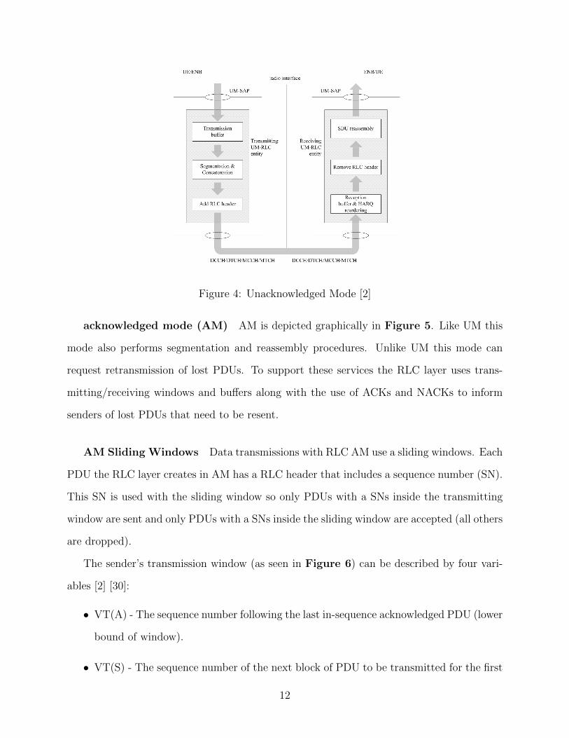
Figure 4: Unacknowledged Mode [2]
acknowledged mode (AM) AM is depicted graphically in Figure 5. Like UM this
mode also performs segmentation and reassembly procedures. Unlike UM this mode can
request retransmission of lost PDUs. To support these services the RLC layer uses trans-
mitting/receiving windows and buffers along with the use of ACKs and NACKs to inform
senders of lost PDUs that need to be resent.
AM Sliding Windows Data transmissions with RLC AM use a sliding windows. Each
PDU the RLC layer creates in AM has a RLC header that includes a sequence number (SN).
This SN is used with the sliding window so only PDUs with a SNs inside the transmitting
window are sent and only PDUs with a SNs inside the sliding window are accepted (all others
are dropped).
The sender’s transmission window (as seen in Figure 6) can be described by four vari-
ables [2] [30]:
• VT(A) - The sequence number following the last in-sequence acknowledged PDU (lower
bound of window).
• VT(S) - The sequence number of the next block of PDU to be transmitted for the first
12
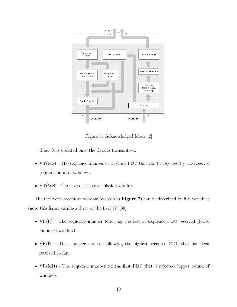
Figure 5: Acknowledged Mode [2]
time. It is updated once the data is transmitted.
• VT(MS) - The sequence number of the first PDU that can be rejected by the receiver
(upper bound of window).
• VT(WS) - The size of the transmission window.
The receiver’s reception window (as seen in Figure 7) can be described by five variables
(note this figure displays three of the five) [2] [30]:
• VR(R) - The sequence number following the last in sequence PDU received (lower
bound of window).
• VR(H) - The sequence number following the highest accepted PDU that has been
received so far.
• VR(MR) - The sequence number for the first PDU that is rejected (upper bound of
window).
13
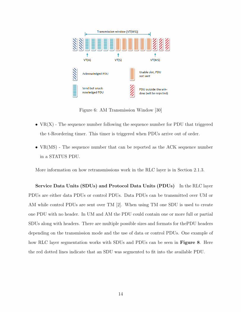
Figure 6: AM Transmission Window [30]
• VR(X) - The sequence number following the sequence number for PDU that triggered
the t-Reordering timer. This timer is triggered when PDUs arrive out of order.
• VR(MS) - The sequence number that can be reported as the ACK sequence number
in a STATUS PDU.
More information on how retransmissions work in the RLC layer is in Section 2.1.3.
Service Data Units (SDUs) and Protocol Data Units (PDUs) In the RLC layer
PDUs are either data PDUs or control PDUs. Data PDUs can be transmitted over UM or
AM while control PDUs are sent over TM [2]. When using TM one SDU is used to create
one PDU with no header. In UM and AM the PDU could contain one or more full or partial
SDUs along with headers. There are multiple possible sizes and formats for thePDU headers
depending on the transmission mode and the use of data or control PDUs. One example of
how RLC layer segmentation works with SDUs and PDUs can be seen in Figure 8. Here
the red dotted lines indicate that an SDU was segmented to fit into the available PDU.
14
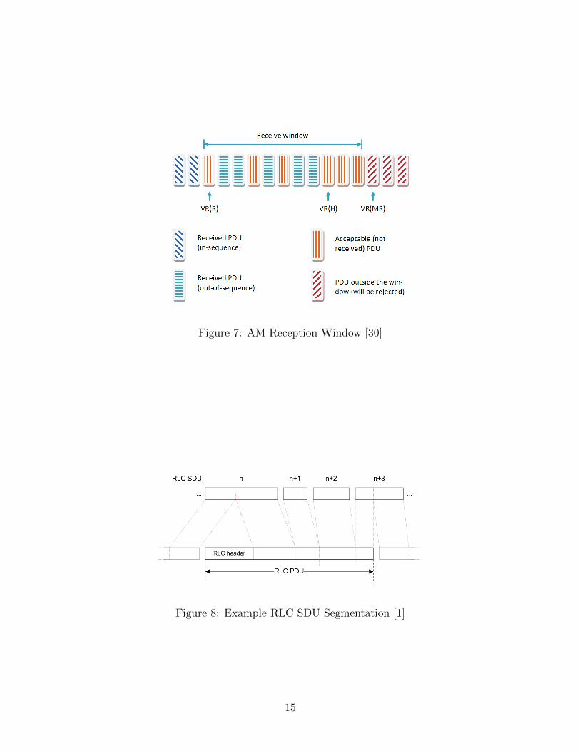
Figure 7: AM Reception Window [30]
Figure 8: Example RLC SDU Segmentation [1]
15

Figure 9: PDCP PDU [1]
2.1.1.4 Packet Data Convergence Protocol (PDCP) Layer
The Packet Data Convergence Protocol (PDCP) layer provides capabilities such as encryp-
tion/decryption, robust header compression for VoIP, integrity protection and SN to provide
duplicate removal [1]. The structure of the PDCP PDU is fairly simple. One PDCP SDU
makes up the payload and the header is either one or two octets long. The structure of this
PDU can be seen in Figure 9. When carrying user data the PDCP SDU will contain one
IP packet.
2.1.1.5 Radio Resource Control (RRC) Layer
The Radio Resource Control (RRC) layer is primarily concerned with the management of
the connections in E-UTRA [1]. This is the highest LTE related layer on a UE. The eNodeB
also has a RRC layer along with the NAS layer.
2.1.1.6 Non Access Stratum (NAS) Layer
The NAS layer exists only on the eNodeB and not on the UEs. Similar to the RRC layer it
handles control functions though at a higher level. The services and functions of the NAS
layer include quality of service (QoS) resource control, handling the mobility of idle devices,
paging origination and the configuration and control of security [1].
16
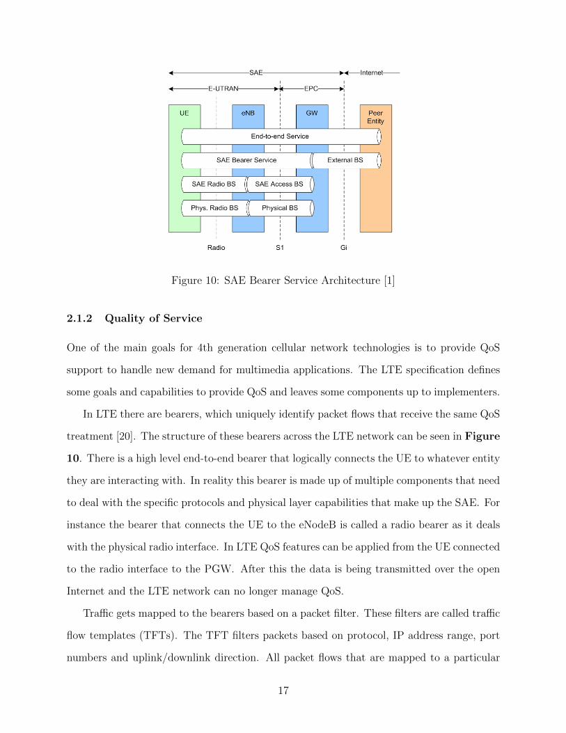
Figure 10: SAE Bearer Service Architecture [1]
2.1.2 Quality of Service
One of the main goals for 4th generation cellular network technologies is to provide QoS
support to handle new demand for multimedia applications. The LTE specification defines
some goals and capabilities to provide QoS and leaves some components up to implementers.
In LTE there are bearers, which uniquely identify packet flows that receive the same QoS
treatment [20]. The structure of these bearers across the LTE network can be seen in Figure
10. There is a high level end-to-end bearer that logically connects the UE to whatever entity
they are interacting with. In reality this bearer is made up of multiple components that need
to deal with the specific protocols and physical layer capabilities that make up the SAE. For
instance the bearer that connects the UE to the eNodeB is called a radio bearer as it deals
with the physical radio interface. In LTE QoS features can be applied from the UE connected
to the radio interface to the PGW. After this the data is being transmitted over the open
Internet and the LTE network can no longer manage QoS.
Traffic gets mapped to the bearers based on a packet filter. These filters are called traffic
flow templates (TFTs). The TFT filters packets based on protocol, IP address range, port
numbers and uplink/downlink direction. All packet flows that are mapped to a particular
17

bearer receive the same packet-forwarding treatment like scheduling, queue management and
other QoS techniques [20]. There is one bearer per QoS class (defined in the next section)
and IP address of the UE [20]. While a UE will have multiple bearers they can be classified
as guaranteed bit rate (GBR) and non-guaranteed bit rate (GBR). As their names suggest
GBR bearers needs to support a minimal bit rate for all of its packet flows while non-GBR
bearers make no such promise [20].
Bearers are also classified based on how they are created. A bearer can be either a default
or dedicated bearer [20]. The default bearer is created when the UE first connects to the
LTE network. This default bearer is also a non-GBR bearer as it must exist no matter
what the network conditions are. Any other bearer that gets created to fill a particular QoS
requirement is considered a dedicated bearer. The TFT of the default bearer allows all traffic
while each dedicated bearer gets a specific TFT to separate its traffic from other flows.
2.1.3 LTE Retransmissions and Applications
For a developer the high bandwidth and QoS considerations in LTE are beneficial for many
applications. However while the LTE specification provides many options there is little the
application developer can do. The only features that the developer can potentially control
that impact LTE are the IP address, port numbers and protocols to use when accessing
content on the Internet. These features can trigger specific radio bearers as discussed in
Section 2.1.2. From the application developers perspective however LTE is a black box.
There is no information on what potential radio bearers are setup or how to access them.
While a phone call is likely to get a high quality of service but a VoIP application a developer
builds cannot indicate what their application needs. There is no information to the developer
on if they will receive AM or UM operations in the RLC layer.
While there is no way for an application developer to know what they will be getting it
would be helpful to know what settings in LTE cause what results on the end application.
This work focuses on settings in the MAC and RLC layers as they deal with retransmissions
18
on the wireless link. For applications we look at examples with delay constraints such as live
voice and video.
2.1.3.1 MAC
As described earlier the MAC layer will attempt to fix lost or damaged data using HARQ.
HARQ is a stop and wait protocol so no new data can be sent until the transmission is
acknowledged. This wait time would add large delays to LTE so the MAC layer compensates
by maintaining multiple HARQ processes in parallel [17]. When frequency division duplexing
(FDD) is used (uplink and downlink are separated by radio frequencies) their are eight
HARQ processes for downlink and uplink traffic. When time division duplexing (TDD) is
used (uplink and downlink are separated by transmission at specific TTIs) the number of
processes for downlink and uplink is dependent on the TDD configuration.
The timing on retransmissions are dependent on if synchronous or asynchronous HARQ
is used. With asynchronous the ID of the specific HARQ process is sent with the ACK or
NACK. This way a receiver can change when they send this control message. With syn-
chronous HARQ the receiver sends the ACK/NACK in a specific subframe, which indicates
the HARQ processes it is associated with. In LTE the downlink uses asynchronous HARQ
while the uplink uses synchronous [17].
For downlink transmissions HARQ will send up to 3 retransmissions [8]. If any of these
packets arrive without error or if any of them run through soft combination (combining
bad PDUs to create the original version) produces a valid packet then the data can be sent
to the RLC layer. If after 3 retransmissions the data cannot be reproduced through soft
combining then it is considered lost. Since multiple processes are sending data and possibly
waiting retransmissions the MAC layer can receive good packets before an earlier bad packet
is corrected. It is up to the higher RLC layer to re-order the data.
Since each HARQ process must wait for an ACK or NACK there is a delay before the
next message can be sent. The delay comes from two times the propagation delay (sending
19
the message from one node to another and then the ACK or NACK) and the time to process
the message at the receiver. Radio waves propagate at the speed of light and since LTE has
to support cells as large as 100km from the tower [17] this translates to a propagation delay
of less than a millisecond.
While the downlink uses asynchronous HARQ and can request retransmissions at an
indeterminate time, there is still a schedule that leads to minimal delay. In FDD there are
eight HARQ processes that transmit one after the next. This means that after a process
transmits it will not get another opportunity until after the other 7 HARQ processes have
sent their data. An example of this is given by [17] and is depicted in Figure 11. Please
note that the transmission and reception windows shown in Figure 11 for the UE are offset.
This is meant to indicate how the UE needs to account for its distance from the eNodeB
and adjust its clock to remain synchronous. This difference is called a timing advance and
is managed with the help of the eNodeB.
The eight processes send a message every subframe (1 ms interval). Say that a HARQ
process at the eNodeB sends its transport block at time n. After a propagation delay the
message arrives at the UE at its time n. The UE then has until time n+4 to determine if an
ACK or NACK is required. At n+4 the UE can send its control message, which arrives at
the eNodeB at its time n+4. At this point a total of 5 HARQ processes could have sent data
leaving another 3 processes to send their data before the original process can either send
new data or resend old at time n+8. This gives us a round trip time of 8 ms for the HARQ
operation when using 8 HARQ processes [17]. If the eNodeB needs to resend the data the
maximum of 3 times then the UE will not get the last retransmission until time n+24. After
processing (3 ms) the final transmission the UE would likely not be able to provide data to
the RLC layer until about 28 ms. Now asynchronous HARQ could be used to change the
order of retransmissions. If this happens however one HARQ process could get a shorter
round trip time (RTT) for its retransmissions at the expense of another process getting an
increased RTT. This example shows how all HARQ processes can be fair to one another.
20
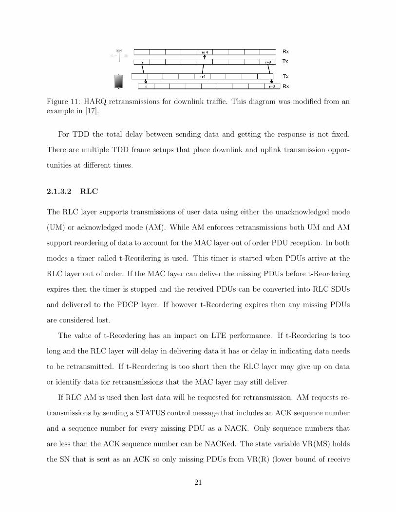
Figure 11: HARQ retransmissions for downlink traffic. This diagram was modified from anexample in [17].
For TDD the total delay between sending data and getting the response is not fixed.
There are multiple TDD frame setups that place downlink and uplink transmission oppor-
tunities at different times.
2.1.3.2 RLC
The RLC layer supports transmissions of user data using either the unacknowledged mode
(UM) or acknowledged mode (AM). While AM enforces retransmissions both UM and AM
support reordering of data to account for the MAC layer out of order PDU reception. In both
modes a timer called t-Reordering is used. This timer is started when PDUs arrive at the
RLC layer out of order. If the MAC layer can deliver the missing PDUs before t-Reordering
expires then the timer is stopped and the received PDUs can be converted into RLC SDUs
and delivered to the PDCP layer. If however t-Reordering expires then any missing PDUs
are considered lost.
The value of t-Reordering has an impact on LTE performance. If t-Reordering is too
long and the RLC layer will delay in delivering data it has or delay in indicating data needs
to be retransmitted. If t-Reordering is too short then the RLC layer may give up on data
or identify data for retransmissions that the MAC layer may still deliver.
If RLC AM is used then lost data will be requested for retransmission. AM requests re-
transmissions by sending a STATUS control message that includes an ACK sequence number
and a sequence number for every missing PDU as a NACK. Only sequence numbers that
are less than the ACK sequence number can be NACKed. The state variable VR(MS) holds
the SN that is sent as an ACK so only missing PDUs from VR(R) (lower bound of receive
21
window) to VR(MS) can be NACKed. The variable VR(H) is the SN after the largest SN
received. VR(H) can be greater than VR(MS).
As new PDUs arrive in sequence VR(R), VR(MS) and VR(MR) are all updated normally.
Once a PDU arrives out of order VR(X) is set to the SN of the PDU that just arrived and
the timer t-Reordering is started. VR(H) is also updated as this is the new highest seen SN.
While t-Reordering is running new PDUs that arrive cause different status variable updates.
As long as the PDU with SN VR(X) does not arrive then VR(R), VR(MR) and VR(MS)
will not update, though VR(H) could. If the missing PDU arrives before the timer expires
then VR(R), VR(MR) and VR(MS) are all updated and the timer is stopped. If however
t-Reordering expires then VR(MS) is updated to the first SN for the PDU after VR(H) for
which not all bytes have been received. This allows for the missing PDU to now b included
as a NACK in a STATUS message. Also when the timer expires if VR(H) is greater than
VR(MS) then other PDUs are missing. If so then t-Reordering are started again. At this
point during the second run of t-Reordering the original missing PDU may arrive. If so then
VR(R) and VR(MR) will be able to update again as it was this original missing PDU that
stopped the lower bound of the receiving window.
For every PDU in AM there is a retransmission count. When a PDU is considered for
retransmission its count is incremented. This makes it up to the transmitter when a PDU
should be abandoned. In AM there is a constant called maxRetxThreshold that identifies
the maximum number of retransmissions for a PDU. However the LTE specification does
not say that a PDU is dropped once its maximum retransmission count is reached. Instead
a message is sent up to the control RRC layer. In the RRC layer the notification of a PDU
reaching its maximum retransmission threshold is considered a radio link failure [5]. When
the UE has detected a radio link failure its RRC layer attempts to reconnect to the RRC
layer at the eNodeB. If a connection is reestablished then the UE releases its RLC and PDCP
entities and existing MAC configuration. This will also cause any existing data received at
the RLC layer but not yet delivered to the higher layers to be lost. This includes all RLC
22

layer data for any other existing connections as well.
The transmitting side of the RLC connection can request a STATUS message through a
poll request. The poll request comes in the form of one bit in the header of a data PDU that
is sent. The transmitter keeps track of two constants to determine when a poll is requested.
These are pollPDU and pollByte. These constants indicate how many PDUs or bytes to
send before requesting a poll for status. A poll is requested whenever one of these constants
is exceeded.
The STATUS message from the receiving RLC AM entity contains the ACKs and NACKs
for the transmitter. The receiving side makes a STATUS message based on a few actions.
First if the timer t-Reordering expires then the receiver will send a STATUS message. Also
the transmitter can request that a STATUS message be sent in the RLC header of transmitted
data. The transmitter keeps track of two state variables, pollPDU and pollByte. These are
maximum the number of PDUs and maximum number of bytes sent between the transmitter
asking for STATUS messages. Once one of these two constants are reached the transmitter
asks for a new STATUS message. At the same time the transmitter will start the timer
t-PollRetransmit. If the STATUS message does not arrive before t-PollRetransmit expires
then the transmitter assumes its poll for STATUS was lost and it sends another. Not only
will the transmitter resend its poll request when the timer expires but it also checks the
status of its buffers. If there is no new data or retransmitted data to send but there is data
pending ACKs then the LTE specification says that the transmitter can either put the last
sent data (VT(S) - 1) into the retransmission buffer, or put all unacknowledged PDUs into
the retransmission buffer.
Another AM timer on the receiver side is is t-StatusProhibit. As long as this timer is
running the RLC layer cannot send any status messages with ACKs or NACKs. This setting
is important because it can delay the RLC layer asking for retransmission and therefore
delay delivering PDUs that have already been received.
23
2.2 ns-3
ns-31 is an open source discrete-event network simulator. ns-3 comes with modules for
simulating network components, protocols and physical transmission methods. The goal of
ns-3 is to improve the core architecture, software integration and educational components
of ns-22. Funding for ns-3 initially came from the National Science Foundation3 and the
Planete4 group at INRIA Sophia Antipolis5. Additional educational and government agencies
have provided founding for ns-3 as well. While ns-2 is still widely used in research the number
of ns-3 users has grown. Between 2009 and 2012 ns-3 was downloaded 50,792 times. As of
the 3.16 release of ns-3 there were 113 listed authors and 25 maintainers of the project6.
One of the modules built into the normal ns-3 distribution is an LTE/EPC Network
Simulator[11]. This module, called LENA, is developed by the Centre Tecnologic de Teleco-
municacions de Catalunya7. Development of the LTE module for ns-3 is ongoing.
The current version of the LTE module allows the creation of simulation networks involv-
ing Internet host connected to cellular phone towers through the EPC that then communicate
over wireless with UEs. In the LTE module users can specify radio bearers for communica-
tion, scheduling algorithms, use of RLC transmission modes, location of towers and other
settings.
Since the LTE module is integrated into ns-3 it can also take advantage of other existing
ns-3 modules. This includes use of normal Internet hosts for UEs to communicate with,
adding buildings to cause obstructions to the propagation of wireless signals, mobility models
to factor movement of UEs, wireless propagation loss models and other features.
1https://www.nsnam.org/2http://nsnam.isi.edu/nsnam/index.php3http://www.nsf.gov/4http://www-sop.inria.fr/planete/index.html5http://www.inria.fr/centre/sophia/6https://www.nsnam.org/overview/statistics/7http://networks.cttc.es/mobile-networks/software-tools/lena/
24
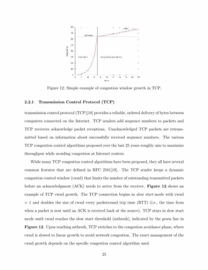
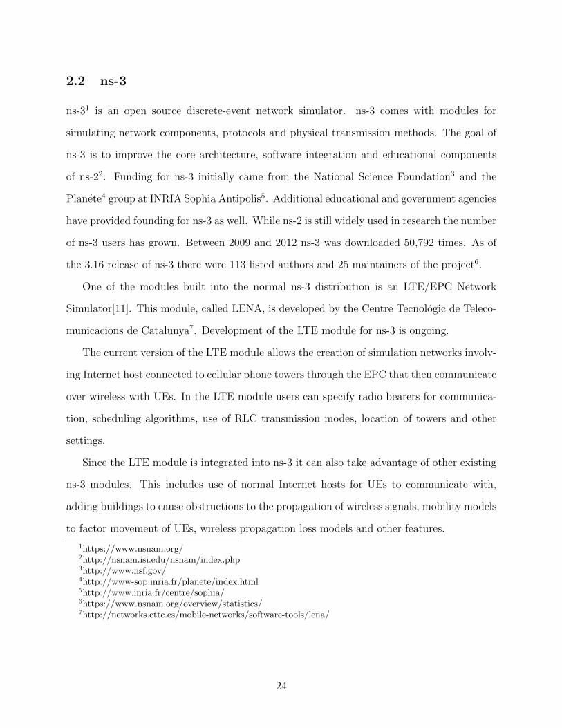
Figure 12: Simple example of congestion window growth in TCP.
2.2.1 Transmission Control Protocol (TCP)
transmission control protocol (TCP)[18] provides a reliable, ordered delivery of bytes between
computers connected on the Internet. TCP senders add sequence numbers to packets and
TCP receivers acknowledge packet receptions. Unacknowledged TCP packets are retrans-
mitted based on information about successfully received sequence numbers. The various
TCP congestion control algorithms proposed over the last 25 years roughly aim to maximize
throughput while avoiding congestion at Internet routers.
While many TCP congestion control algorithms have been proposed, they all have several
common features that are defined in RFC 2581[19]. The TCP sender keeps a dynamic
congestion control window (cwnd) that limits the number of outstanding transmitted packets
before an acknowledgment (ACK) needs to arrive from the receiver. Figure 12 shows an
example of TCP cwnd growth. The TCP connection begins in slow start mode with cwnd
= 1 and doubles the size of cwnd every packetround trip time (RTT) (i.e., the time from
when a packet is sent until an ACK is received back at the source). TCP stays in slow start
mode until cwnd reaches the slow start threshold (ssthresh), indicated by the green line in
Figure 12. Upon reaching ssthresh, TCP switches to the congestion avoidance phase, where
cwnd is slowed to linear growth to avoid network congestion. The exact management of the
cwnd growth depends on the specific congestion control algorithm used.
25
As of version 3.19, ns-3 natively supports the congestion control algorithms are Reno,
NewReno, Tahoe, Westwood and Westwood+. There are also software modules for ns-3 that
can provide access to the operating systems TCP stack but this is only supported on some
systems and does not provide the fine grained logging of the native ns-3 code.
2.2.2 User Datagram Protocol (UDP)
user datagram protocol (UDP)[34] provides delivery of bytes between computers connected
on the Internet with a minimal protocol overhead. This protocol only defines the source
port, destination port, length of the data and a checksum along with the message. There
is no reliable delivery of data with UDP. If a packet is lost then it cannot be recovered.
UDP is meant for applications that do not require any reliability in a message reaching its
destination. The low overhead of UDP makes it ideal for real time applications where the
delay of waiting for the retransmission of data is unacceptable.
2.3 Applications
2.3.1 VoIP
Voice over IP (VoIP) and conversational video allow users to communicate with each other
over the Internet in real time. Providing a good QoS for these types of applications is
measured by the quality of the communication the users have. Does the user experience
lost parts of the conversation? Does it take too long to receive data that the users are left
waiting for responses? Is the audio and video clear and understandable? This section briefly
introduces some basic components to VoIP and conversational video systems and discusses
what can be considered a good QoS.
While there are many protocols and technologies for manipulating audio and video data
they all follow a few fundamental steps. When a source has audio or video data to send it
first encodes it into binary data for transmission. The type of encoding used could employ
26
techniques to recover lost data or minimize the size. The sender then packetizes the data and
sends it. The receiver normally keeps a buffer to hold incoming data. The buffer is used to
provide a steady playback as the arrival of data is subject to network delays. The data is then
decoded and presented to the user. In general the sources for delay are encoding/decoding,
packetization, network latency and buffering [28] [10].
The choice of encoder impacts how much data is generated and the rate of transmission
needed for the conversation. While there are many types of encoders one common example
is G.711 [36]. This coded creates 160 bytes of application data. This is encapsulated in a
real time protocol (RTP) packet with a 12 byte header to provide some timing information
on how to play out the data. This is placed in a UDP packet (8 byte header) and then in
an IP frame (20 byte header). This codec transmit data every 20 ms creating a data rate of
64Kb/s.
For users on either end of a connection to maintain a conversation either through VoIP
or video they need to receive data quickly with a minimum of loss. Unfortunately packet
loss and transmission delays are at odds with one another. TCP provides reliable delivery
through retransmissions, which adds delay. UDP adds minimal overhead to data, which
improves delay but lost data cannot be recovered. Holding live conversations are more
sensitive to delay than packet loss [15]. The International Telecommunication Union (ITU)
recommends that one way delay should be less than 400 ms at most while a limit of 150 ms
would allow most applications to run without any users realizing the delay[39].
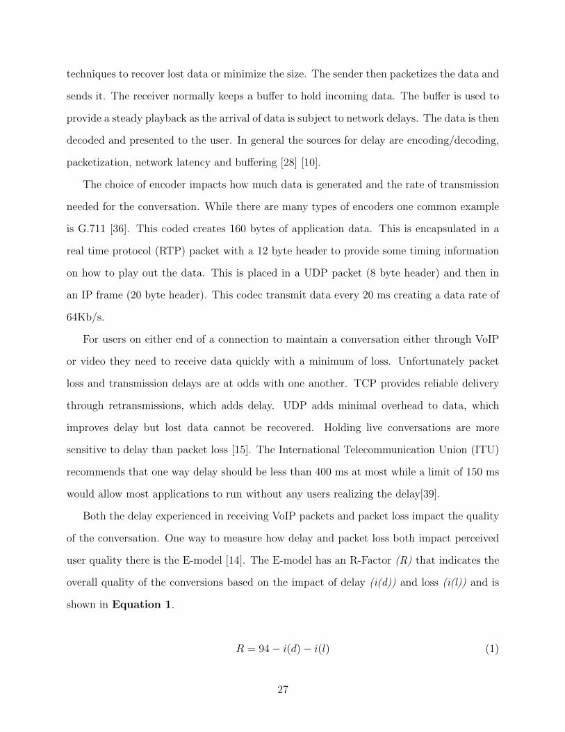
Both the delay experienced in receiving VoIP packets and packet loss impact the quality
of the conversation. One way to measure how delay and packet loss both impact perceived
user quality there is the E-model [14]. The E-model has an R-Factor (R) that indicates the
overall quality of the conversions based on the impact of delay (i(d)) and loss (i(l)) and is
shown in Equation 1.
R = 94 − i(d) − i(l) (1)
27

Table 3: Listening Quality Scale with MOS [37]
Speech Quality MOSExcellent 5Good 4Fair 3Poor 2Bad 1
The impact from delay is calculated from Equation 2. Here the one way delay (d) is
used in two different equations depending on if the delay is smaller or larger than 177.3 ms.
i(d) =
0.024 × d d ≤177.3
0.024 × d + 0.11 × (d− 177.3) d >177.3(2)
The impact from packet loss, (i(l)) is calculated using Equation 3.
i(l) = 30 × log(1 + 15 × l) (3)
The result of Equation 1 produces a number from 0 to 94. 94 is the best quality while 0
is the worst. This value can then be used to calculate a G-Model mean opinion score (MOS)
[12]. The MOS was originally created as a metric for getting a users opinion of voice call
quality. The ITU outlines how to map the R value to the MOS in [38]. R values less than
0 make a MOS of 1. Values between 0 and 100 are set using Equation 4. Any R value
greater than 100 results in a MOS of 5. Equation 1 can only create an R value as high as
94 but this is because this particular equation for the E-Model R factor is slightly different
than others. The original MOS ranges from 1 - 5 as seen in Table 3. Equation 4 will only
produce a maximum MOS of 4.5.
E(R) = 1.0 + 0.035 ×R + 0.000007 ×R× (R− 60) × (100 −R) (4)
28
2.3.2 FTP
file transfer protocol (FTP) is a protocol for transferring a file from one computer to another
over a network. FTP creates a connection from one host to another and sends the contents
of a file using TCP to ensure all of the entire file arrives at the receiver without error. While
FTP is not concerned with delay like a VoIP or a video application is it is concerned with the
overall throughput available to it. TCP will transfer data as fast as possible on the network
so the current capacity of a network determines how much TCP can send and therefore how
long it will take to transfer the entire file. FTP is a simple example for a TCP application
to use in comparison with the VoIP and video applications. The TCP throughput is used to
measure application performance.
2.3.3 Video
A video is just a series of pictures presented at a particular frame rate (there is also the audio
component but the largest part of the data is the image). When the pictures are presented
at a particular frame rate a viewer perceives motion by the changes in the picture. Video
compression techniques take advantage of the fact that not all of the information in every
picture is required. While there are multiple video encoding formats the examples used in
this work use MPEG [22]. MPEG relies on temporal and spatial redundancy reduction. The
idea is that across time and space (part of the image) there is content that is duplicated
across frames that could be removed. In MPEG there are three types of frames, I, P and
B. The I frame has the least amount of compression and provides a basic image. A P frame
references a previously seen I frame and denotes what content in the image has changed
for the future. A B frame also indicates portions of an image that change but it refers to
previous and upcoming frames. MPEG then encodes a video into a series of I, P and B
frames to reduce the total amount of data needed for the video. While the P and B frames
denote changes there are still multiple I frames with a larger copy of the image. This is so
video playback can provide random access [22]. A similar idea of removing redundant parts
29
of images that either cannot be detected or can be recreated by the player is a part of many
video compression schemes. The frame rate at the receiver is used to measure application
performance.
30
3 Related Work
As cellular networks and mobile devices have become more common in society, research
into these areas has been ongoing. This section covers research in mobile applications and
aspects of LTE. First, research into mobile applications shows that communication focus
is prominent for users. Research into LTE is then considered. This includes measurements
of real application data in LTE networks, some aspects of wireless retransmissions and a
specific look at VoIP in LTE.
3.1 Applications in Cellular Networks
Xu et al. [41] examines the types of applications used by phones across the US by a tier-1
cellular network provider. The data set for this study was collected from all links within
the tier-1 network from the radio access (cell phone towers) to the Internet. This data was
collected over one week in August 2010. The authors found that 20% of mobile applications
dealt with content local to the users such as news and radio stations for the area around the
user’s location. They also found that certain applications were likely to be used together
(one after another) like multiple news applications. Many applications had identifiable usage
patterns. News applications are used more in the morning for instance. Other applications
like games are more likely when the user is traveling, e.g., while waiting in an airport.
One important finding related to this work is that the top data consumer application was
a personalized Internet radio, which was responsible for more than 3 TB of data over the
week. This shows that streaming audio is a popular application for mobile devices.
Bohmer et al. [13] studied the applications users ran on their mobile phones and how
they used them. The authors created an Android application that collected data on when
applications were installed, opened, closed, updated and installed. The application sent
this data back to the authors to use for their study. To encourage users to participate
the application would also make recommendations on other applications the user may be
31
interested in. The authors collected data for 4,125 users from August 2010 to January 2011.
They found that, on average, users spend 59.23 minutes per day on their mobile devices. The
authors found that mobile application were also most likely used for communication through
phone calls, emails, texts and other communication applications. This research shows that
communication type applications that are delay sensitive are used regularly.
3.2 LTE Measurements
Huang et al. [25] examined data collected from an LTE network in a US city in October
2012 amounting to 2.9 TB of data. The authors characterized the network protocols, network
characteristics and types of applications used in the dataset. They found that TCP made
up 95.3% of traffic flows and 97.2% of bytes. The majority of the remaining flows and bytes
used UDP. Downlink data sent from the tower to the phone took up the majority of the data
in the network. Of the top 5% of flows (by payload size) 74.4% were related to video or audio
applications. One result of this research is that the RTT from the LTE network to the UE
was shorter than the RTT of the LTE network to external Web servers. The authors reported
the normalized RTT for connection going from the UE to a monitoring node inside the LTE
network and then connections from the monitoring node to the external server handling the
application request. For about 40% of all data collected, the RTT of the connection from
the UE to the monitoring node was larger than from the monitoring node to the external
server. For the rest of the data collected the RTT from the UE to the monitor was smaller
than from the monitor to the external server. The authors also found that 38.1% of TCP
flows did not have any TCP layer retransmissions. While Huang et al [25] collected a large
volume of real data, they did not have access to data from the LTE network layers. We do
not know what RLC settings the networks used or how many PRBs were available.
Jiang et a.l [27] examined TCP performance in 3G and 4G networks including LTE.
Their measurements show the existence of large buffers in cellular networks leading to buffer
bloat problems. The authors found that at least for the Android operating system (which
32
is open source) the maximum window size for TCP was a static setting based on the type
of network used. The reason for this is to limit the number of bytes in flight to reduce the
increased RTT due to having large buffers. The idea is that the more data gets pushed
through the network the more data has to sit in buffers meaning the time to get the data
increases. This issue was found in both a AT&T HSPA+ 3G network and a Verizon LTE
4G network. The LTE network had higher throughput and lower RTTs compared to the 3G
network but both have problems due to the static maximum TCP window size. The authors
proposed an algorithm that would dynamically adjust the maximum window size to balance
throughput and RTT concerns. This work shows how throughput and latency issues are still
a concern in existing LTE networks. While this work looked at making adjustments to TCP,
there is no information on the configuration of the underlying LTE network that handled
the traffic.
3.3 HARQ
Kawser et al. [29] looked at saving radio resources by limiting the maximum number of
HARQ retransmissions. Their reasoning was that for nodes experiencing poor radio con-
ditions having three retransmissions would not provide a successful retransmission or soft
combining to recover the lost data. The authors used an LTE link layer simulator to exam-
ine the difference in the BLER of the wireless transmission with bad SINR. Their results
show only a small performance improvement for the full three retransmissions. The authors
instead suggest that for poor radio conditions only one or two retransmissions should be
allowed in HARQ. This work only looks at performance related to the MAC layer HARQ
process. It does not include any retransmissions from the RLC layer, nor does it show how
these retransmissions and delays impact high level applications.
Ikuno et al. [26] examined how HARQ layer retransmissions create a SINR shift in the
BLER curve. In LTE, a BLER of 10% or less is the target used to set the modulation and
encoding scheme. The received SINR at the UE is used to create BLER curves showing
33
what the expected BLER is for different SINRs. As the SINR worsens the BLER increases.
Changing the modulation and encoding scheme moves the BLER curve, for example, going
from 64 to 16 quadrature amplitude modulation (QAM) would move the the curve so the
same SINR would have a lower BLER. The authors developed a model that takes into
account the number of HARQ retransmissions and the current modulation scheme to pre-
dict the SINR gain in decibels. When compared to simulations run using a Matlab based
downlink physical layer simulator [32], this work showed an error rate in predicting the SINR
improvement of less than 1% for QPSK and 16 QAM but a 11% error rate for 64 QAM. This
work does not look at any of the possible applications of this research but with the ability to
better predict the improvements from HARQ retransmissions, a system could make better
decisions on how to transfer data
3.4 RLC
Makidis [30] implemented and evaluated RLC AM for his Master’s thesis. The author im-
plemented their RLC AM in ns-2 and tested with TCP based application like Web browsing
with hypertex transfer protocol (HTTP) and FTP traffic. Simulations showed that using
RLC AM works well with applications that experience contention. Comparing RLC AM with
two other selective repeat protocols showed that the adaptive selective repeat is preferred
when maximizing TCP throughput. The throughput for Web browsing traffic in RLC AM
was significantly lower than both the selective repeat variants. RLC AM performed better
when dealing with large file transfers with FTP.
While Makdis implemented the RLC AM protocol in ns-2, he did not implement the
other LTE layers. This is problematic as the loss rate applied to these simulations do not
take the MAC layer HARQ retransmissions into account. The author did not implement
the RLC UM or run any tests with this option. This is possibly because the author was
trying to show the impact of retransmissions, but the MAC layer would have provided
retransmissions for comparison. Since the author stated that the RLC parameters he used
34

were shown experimentally to have good results, there was no adjusting of these parameters
to show what changes would occur to the end results.
3.5 VoIP in LTE
Asheralieva et al. [9] simulated running VoIP applications over LTE. These authors focused
on two packet scheduling mechanisms and if HARQ was used or not. The authors’ found
that HARQ can improve QoS for VoIP services. These authors simulation took into account
scheduling along with the physical and MAC layers. They did not include the RLC layer
that would handle reordering of packets during packet loss. They also did not consider at if
the RLC layer was enforcing retransmission of lost packets.
Masum et al. [31] examined the end-to-end delay of VoIP applications in LTE networks.
The authors used the OPNET simulator and created example networks to examine a baseline
VoIP network, a congested VoIP network and a VoIP congested network with an FTP traffic
mix. In these scenarios the authors modified speed of UEs, packet loss and the available
bandwidth (changing the number of available PRBs). They found that when there is no
movement the end-to-end delay is slightly higher for networks congested with only VoIP
traffic, however the authors do not examine why their simulations produced these results. In
the other scenarios the end-to-end delay was better when nodes were mobile. In congested
VoIP networks the speed of the mobile UEs had little impact on packet loss. For the network
with mixed FTP traffic, stationary nodes saw little packet loss while mobile nodes saw more.
While the work of Masum et al shows the delay perceived in VoIP over LTE, they did
not adjust any of the settings in the RLC layer. They also did not report any information
about performance in the MAC or RLC layers. The highest average packet loss across their
tests was less than 4%.
35
4 Approach
4.1 Problem Statement
The LTE specification allows for retransmissions in both the MAC and RLC layer. The MAC
layer retransmissions recover most lost packets with low latency while the RLC layer adds
retransmissions to keep wireless error rates below 1% to improve TCP performance [17]. The
use of QoS classes and radio bearers allow for multiple RLC entities and potentially multiple
configurations for the use of AM/UM and other configurations. However, network providers
do not publish information on what their QoS setups are and data flows can only be classified
by their protocol, IP addresses, ports used and the direction of traffic (uplink/downlink). As
it stands the application developer does not know if the application is connected through the
RLC AM for higher reliability or through UM for lower latency. There is also no information
for the developer on what settings are being used inside the RLC layer for timeouts or status
messages.
As an example assume a developer knows their application will need to send sets of
messages in bursts. It may be best if this string of messages is not interrupted by RLC AM
STATUS messages. If the LTE network posted its QoS classes and the RLC layer settings
the developer could potentially setup the protocol and port numbers their applications use to
ensure the traffic gets sent to the QoS class with the best RLC settings for their application.
4.1.0.1 Objectives
This work examines how adjustments to the configurable parameters in the RLC layer im-
pacts application level performance for applications. Specifically, this work looks at applica-
tions with different QoS concerns and characteristics. VoIP applications need to keep both
a low delay and low packet loss rate while sending a small amount of data at a relatively
low rate. FTP applications are mostly concerned with throughput so files can be moved
36
as quickly as possible and without any loss. Video applications send large amounts of data
that require a low amount of packet loss. However the format of the video adds additional
concerns. A video for a live conversation like a video conference will be concerned with the
delay on arriving video frames and will allow some packet loss. A video of a past recorded
event like a movie on the other hand can use a playout buffer to compensate for more delay
while expecting few if any packets to be lost. The following outlines how we will test these
applications within LTE.
4.1.0.2 VoIP with varied RLC settings
Test a VoIP application with different settings for t-Reordering and t-StatusProhibit timers.
Methods Configure ns-3 simulations to use a constant bit rate application that uses
UDP. The application is designed to send traffic at a constant rate of 64 Kb/s to align
with the G.711 encoding standard [36]. Simulation runs use AM and UM with different
settings for the t-Reordering and t-StatusProhibit timer with some wireless loss. The delay
of arriving UDP packets and percent of packet lost is used to calculate the MOS to determine
the settings for these timers that produce the best results.
4.1.0.3 VoIP with AM vs UM with varied loss
Test a VoIP application with constant settings in RLC AM and UM with different amounts
of loss.
Methods Using the same application setup for testing the RLC layer settings this test
compares using the preferred settings found previously with a varied amount of wireless loss
to find under what conditions AM or UM perform better. Once again the MOS is used to
determine the overall quality of the conversation.
37
4.1.0.4 FTP with varied RLC settings
Test the performance of transferring a file from a server to a UE using varied RLC settings.
Methods Configure ns-3 simulations to use an FTP -like application where TCP New
Reno is used to send as much data as possible from a server to the UE. The settings for the
t-Reordering and t-StatusProhibit are varied with AM and UM to find settings that produce
the highest throughput for the application.
4.1.0.5 FTP with AM vs UM with varied loss
Test the performance of transferring a file from a server to a UE using both AM and UM
with different amounts of loss.
Methods Using the preferred settings for t-Reordering and t-StatusProhibit run the
FTP simulation for both AM and UM with a varied amount of wireless loss to find under
what condition AM or UM perform better based on the application throughput.
4.1.0.6 MPEG video with varied RLC settings
Test the performance of MPEG video transferring from a server to the UE using varied RLC
settings.
Methods Configure ns-3 simulations to use an MPEG UDP application. The applica-
tion is designed to send UDP packets based on a trace file from a real MPEG-4 encoding of
a video. These simulations adjust the settings for t-Reordering and t-StatusProhibit timers
long with using AM and UM to find reasonable settings for these timers.
4.1.0.7 MPEG video with AM vs UM
Test the performance of MPEG videos when using AM and UM and varying loss.
38
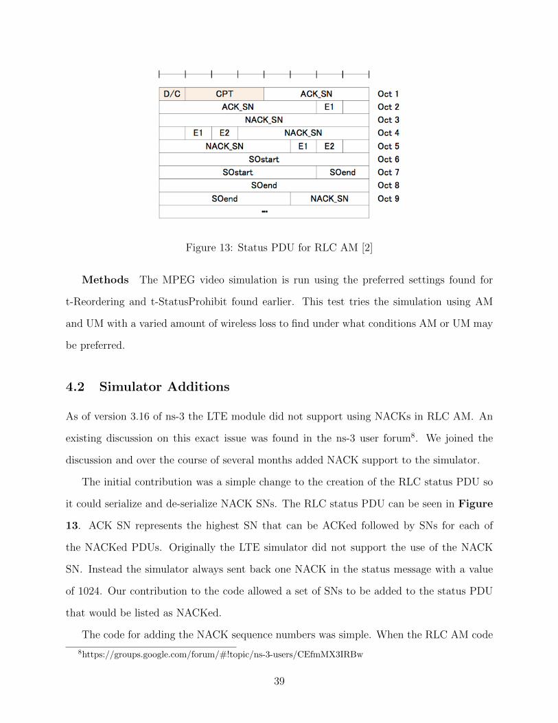
Figure 13: Status PDU for RLC AM [2]
Methods The MPEG video simulation is run using the preferred settings found for
t-Reordering and t-StatusProhibit found earlier. This test tries the simulation using AM
and UM with a varied amount of wireless loss to find under what conditions AM or UM may
be preferred.
4.2 Simulator Additions
As of version 3.16 of ns-3 the LTE module did not support using NACKs in RLC AM. An
existing discussion on this exact issue was found in the ns-3 user forum8. We joined the
discussion and over the course of several months added NACK support to the simulator.
The initial contribution was a simple change to the creation of the RLC status PDU so
it could serialize and de-serialize NACK SNs. The RLC status PDU can be seen in Figure
13. ACK SN represents the highest SN that can be ACKed followed by SNs for each of
the NACKed PDUs. Originally the LTE simulator did not support the use of the NACK
SN. Instead the simulator always sent back one NACK in the status message with a value
of 1024. Our contribution to the code allowed a set of SNs to be added to the status PDU
that would be listed as NACKed.
The code for adding the NACK sequence numbers was simple. When the RLC AM code
8https://groups.google.com/forum/#!topic/ns-3-users/CEfmMX3IRBw
39
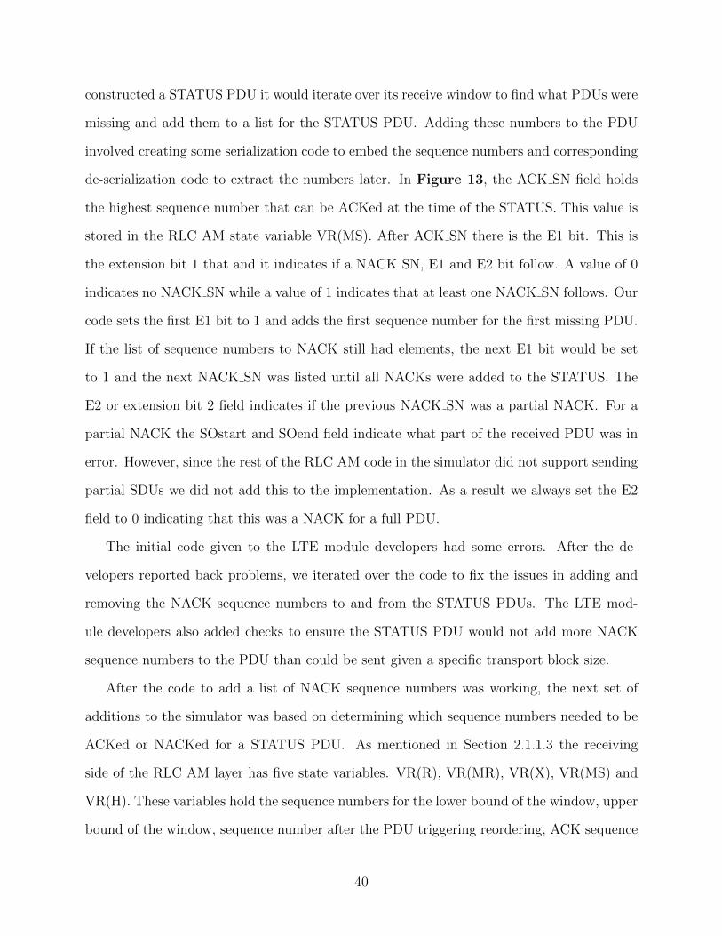
constructed a STATUS PDU it would iterate over its receive window to find what PDUs were
missing and add them to a list for the STATUS PDU. Adding these numbers to the PDU
involved creating some serialization code to embed the sequence numbers and corresponding
de-serialization code to extract the numbers later. In Figure 13, the ACK SN field holds
the highest sequence number that can be ACKed at the time of the STATUS. This value is
stored in the RLC AM state variable VR(MS). After ACK SN there is the E1 bit. This is
the extension bit 1 that and it indicates if a NACK SN, E1 and E2 bit follow. A value of 0
indicates no NACK SN while a value of 1 indicates that at least one NACK SN follows. Our
code sets the first E1 bit to 1 and adds the first sequence number for the first missing PDU.
If the list of sequence numbers to NACK still had elements, the next E1 bit would be set
to 1 and the next NACK SN was listed until all NACKs were added to the STATUS. The
E2 or extension bit 2 field indicates if the previous NACK SN was a partial NACK. For a
partial NACK the SOstart and SOend field indicate what part of the received PDU was in
error. However, since the rest of the RLC AM code in the simulator did not support sending
partial SDUs we did not add this to the implementation. As a result we always set the E2
field to 0 indicating that this was a NACK for a full PDU.
The initial code given to the LTE module developers had some errors. After the de-
velopers reported back problems, we iterated over the code to fix the issues in adding and
removing the NACK sequence numbers to and from the STATUS PDUs. The LTE mod-
ule developers also added checks to ensure the STATUS PDU would not add more NACK
sequence numbers to the PDU than could be sent given a specific transport block size.
After the code to add a list of NACK sequence numbers was working, the next set of
additions to the simulator was based on determining which sequence numbers needed to be
ACKed or NACKed for a STATUS PDU. As mentioned in Section 2.1.1.3 the receiving
side of the RLC AM layer has five state variables. VR(R), VR(MR), VR(X), VR(MS) and
VR(H). These variables hold the sequence numbers for the lower bound of the window, upper
bound of the window, sequence number after the PDU triggering reordering, ACK sequence
40
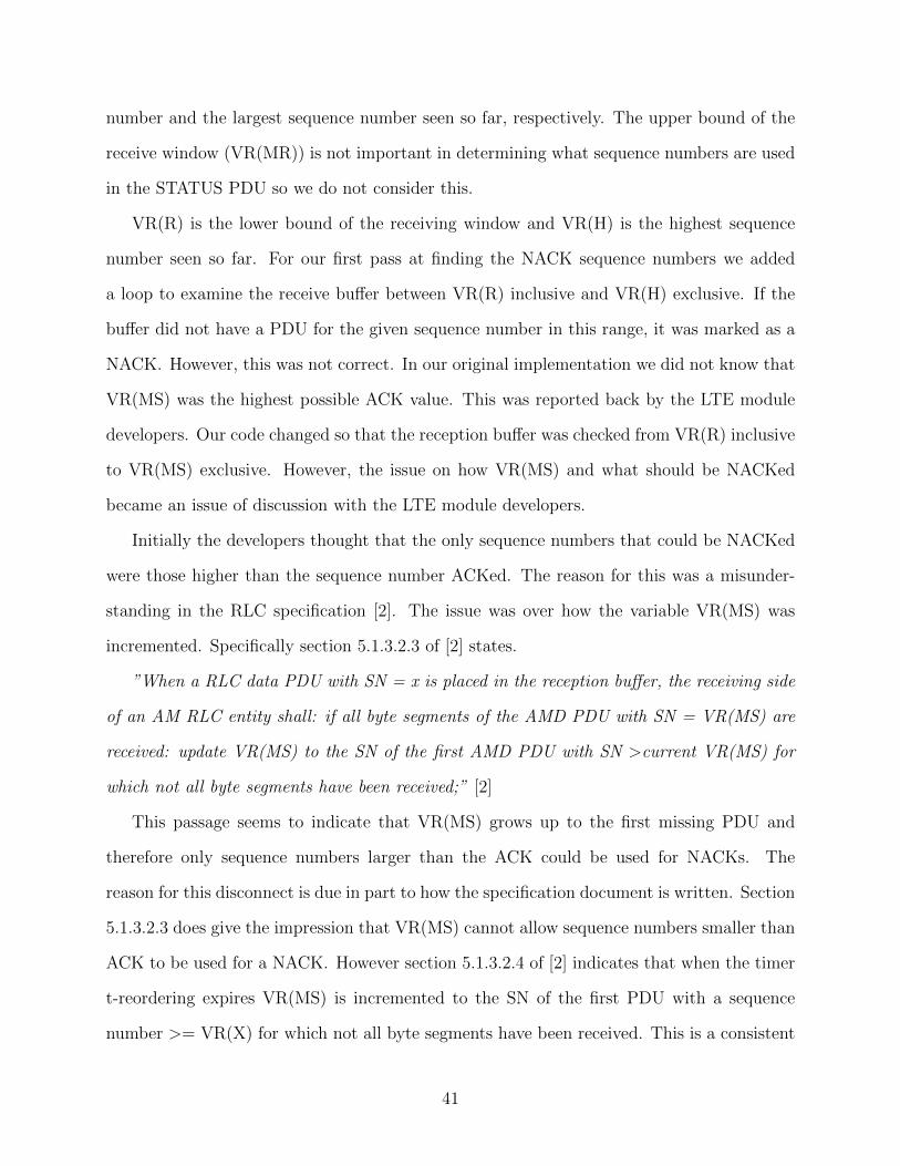
number and the largest sequence number seen so far, respectively. The upper bound of the
receive window (VR(MR)) is not important in determining what sequence numbers are used
in the STATUS PDU so we do not consider this.
VR(R) is the lower bound of the receiving window and VR(H) is the highest sequence
number seen so far. For our first pass at finding the NACK sequence numbers we added
a loop to examine the receive buffer between VR(R) inclusive and VR(H) exclusive. If the
buffer did not have a PDU for the given sequence number in this range, it was marked as a
NACK. However, this was not correct. In our original implementation we did not know that
VR(MS) was the highest possible ACK value. This was reported back by the LTE module
developers. Our code changed so that the reception buffer was checked from VR(R) inclusive
to VR(MS) exclusive. However, the issue on how VR(MS) and what should be NACKed
became an issue of discussion with the LTE module developers.
Initially the developers thought that the only sequence numbers that could be NACKed
were those higher than the sequence number ACKed. The reason for this was a misunder-
standing in the RLC specification [2]. The issue was over how the variable VR(MS) was
incremented. Specifically section 5.1.3.2.3 of [2] states.
”When a RLC data PDU with SN = x is placed in the reception buffer, the receiving side
of an AM RLC entity shall: if all byte segments of the AMD PDU with SN = VR(MS) are
received: update VR(MS) to the SN of the first AMD PDU with SN >current VR(MS) for
which not all byte segments have been received;” [2]
This passage seems to indicate that VR(MS) grows up to the first missing PDU and
therefore only sequence numbers larger than the ACK could be used for NACKs. The
reason for this disconnect is due in part to how the specification document is written. Section
5.1.3.2.3 does give the impression that VR(MS) cannot allow sequence numbers smaller than
ACK to be used for a NACK. However section 5.1.3.2.4 of [2] indicates that when the timer
t-reordering expires VR(MS) is incremented to the SN of the first PDU with a sequence
number >= VR(X) for which not all byte segments have been received. This is a consistent
41
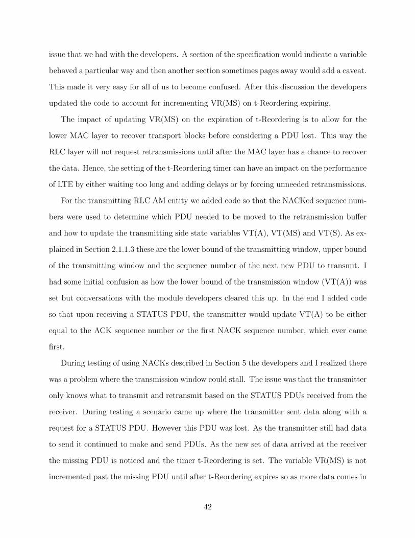
issue that we had with the developers. A section of the specification would indicate a variable
behaved a particular way and then another section sometimes pages away would add a caveat.
This made it very easy for all of us to become confused. After this discussion the developers
updated the code to account for incrementing VR(MS) on t-Reordering expiring.
The impact of updating VR(MS) on the expiration of t-Reordering is to allow for the
lower MAC layer to recover transport blocks before considering a PDU lost. This way the
RLC layer will not request retransmissions until after the MAC layer has a chance to recover
the data. Hence, the setting of the t-Reordering timer can have an impact on the performance
of LTE by either waiting too long and adding delays or by forcing unneeded retransmissions.
For the transmitting RLC AM entity we added code so that the NACKed sequence num-
bers were used to determine which PDU needed to be moved to the retransmission buffer
and how to update the transmitting side state variables VT(A), VT(MS) and VT(S). As ex-
plained in Section 2.1.1.3 these are the lower bound of the transmitting window, upper bound
of the transmitting window and the sequence number of the next new PDU to transmit. I
had some initial confusion as how the lower bound of the transmission window (VT(A)) was
set but conversations with the module developers cleared this up. In the end I added code
so that upon receiving a STATUS PDU, the transmitter would update VT(A) to be either
equal to the ACK sequence number or the first NACK sequence number, which ever came
first.
During testing of using NACKs described in Section 5 the developers and I realized there
was a problem where the transmission window could stall. The issue was that the transmitter
only knows what to transmit and retransmit based on the STATUS PDUs received from the
receiver. During testing a scenario came up where the transmitter sent data along with a
request for a STATUS PDU. However this PDU was lost. As the transmitter still had data
to send it continued to make and send PDUs. As the new set of data arrived at the receiver
the missing PDU is noticed and the timer t-Reordering is set. The variable VR(MS) is not
incremented past the missing PDU until after t-Reordering expires so as more data comes in
42
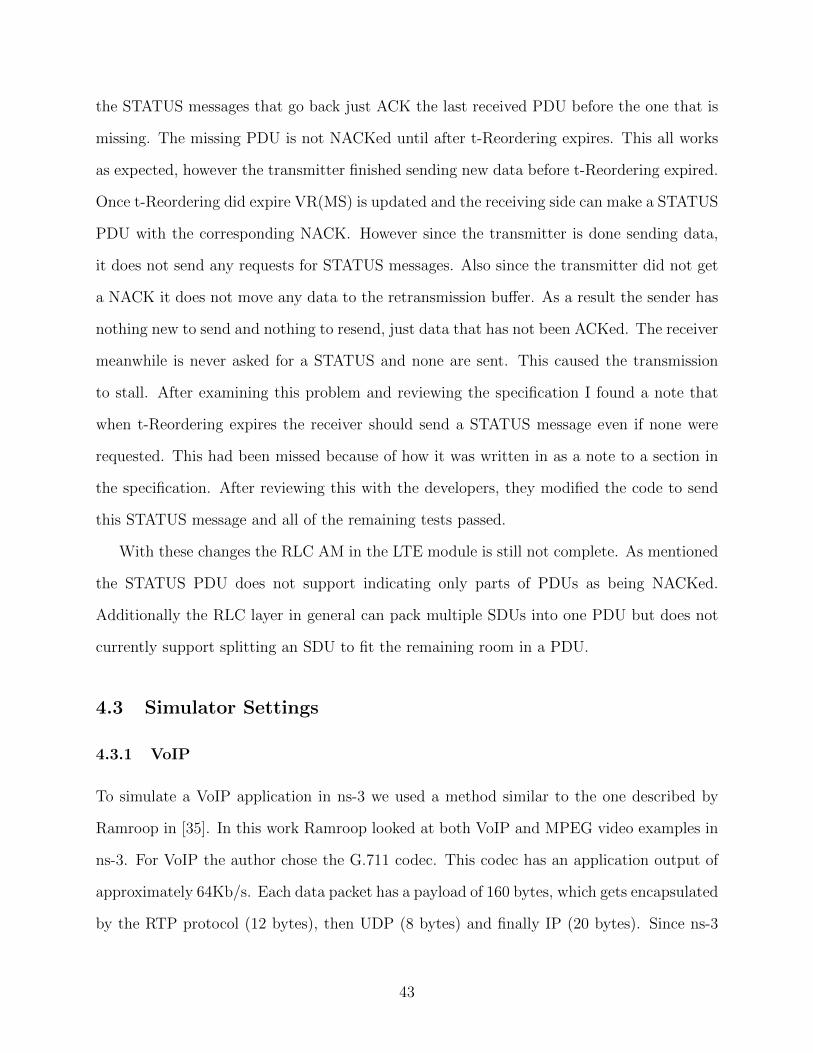
the STATUS messages that go back just ACK the last received PDU before the one that is
missing. The missing PDU is not NACKed until after t-Reordering expires. This all works
as expected, however the transmitter finished sending new data before t-Reordering expired.
Once t-Reordering did expire VR(MS) is updated and the receiving side can make a STATUS
PDU with the corresponding NACK. However since the transmitter is done sending data,
it does not send any requests for STATUS messages. Also since the transmitter did not get
a NACK it does not move any data to the retransmission buffer. As a result the sender has
nothing new to send and nothing to resend, just data that has not been ACKed. The receiver
meanwhile is never asked for a STATUS and none are sent. This caused the transmission
to stall. After examining this problem and reviewing the specification I found a note that
when t-Reordering expires the receiver should send a STATUS message even if none were
requested. This had been missed because of how it was written in as a note to a section in
the specification. After reviewing this with the developers, they modified the code to send
this STATUS message and all of the remaining tests passed.
With these changes the RLC AM in the LTE module is still not complete. As mentioned
the STATUS PDU does not support indicating only parts of PDUs as being NACKed.
Additionally the RLC layer in general can pack multiple SDUs into one PDU but does not
currently support splitting an SDU to fit the remaining room in a PDU.
4.3 Simulator Settings
4.3.1 VoIP
To simulate a VoIP application in ns-3 we used a method similar to the one described by
Ramroop in [35]. In this work Ramroop looked at both VoIP and MPEG video examples in
ns-3. For VoIP the author chose the G.711 codec. This codec has an application output of
approximately 64Kb/s. Each data packet has a payload of 160 bytes, which gets encapsulated
by the RTP protocol (12 bytes), then UDP (8 bytes) and finally IP (20 bytes). Since ns-3
43
does not have a module for RTP the author added the 12 bytes of RTP header to the data
packet for a size of 172 bytes. These are then encapsulated by UDP and IP as supported
in ns-3. To simulate a VoIP conversation, Ramroop used an on/off ns-3 application that
allows control either directly or through a random value (with a specified mean) when to
turn sending on and off. For simplicity we decided to make our VoIP example a simple
constant bit rate. This is not like a real VoIP conversation but since we are interested on
the delay of packet arrival and loss, it is an acceptable trade off.
In ns-3 we created a constant bit rate (CBR) sending UDP application. We set the
payload size in bytes to be 172 bytes (160 bytes of data and 12 of RTP header) and set an
interval on sending packets of 0.02 seconds to generate 50 packets per second.
4.3.2 FTP
To simulate FTP, ns-3 has a bulk send application that transfers data as fast as possible
using TCP. The application sets the maximum number of bytes to transfer, allowing the
simulation to send files of varied sizes. The TCP stack in ns-3 supports only a few of the
early TCP congestion control algorithms. These are Reno, NewReno, Tahoe, Westwood and
Westwood+. ns-3 does support accessing the TCP stack of the operating system through
extensions like the network simulation cradle (NSC) and direct code execution (DCE). While
NSC and DCE allows the use of modern TCP implementations, these components are not
part of the default ns-3 and do not work on all operating systems. Attempts to use NSC with
the LTE module caused the TCP simulations to end before sending all data. The reason
for this error is unknown and there was not enough time to thoroughly examine the cause.
Similarly, there was not enough time to examine how DCE could be used. As a result these
simulations use the ns-3 default of NewReno. This means that the TCP implementation will
take longer to fill the congestion window, opposed to newer algorithms.
44

Table 4: MPEG frame trace.
Frame No. FrameType Time[ms] Length[byte]1 I 0 75592 P 120 34423 B 40 18654 B 80 20215 P 240 22826 B 160 15327 B 200 18538 P 360 22169 B 280 151510 B 320 1664
4.3.3 Video
For video we use a sample application that comes with ns-3. This applications takes as its
input a trace file that defines an MPEG 4 video. The trace file lists four columns for a
row number, frame type, time to send the packet and size of the packet in bytes as seen in
Table 4. Example trace files for this application are available from the Telecommunications
Network Group at the Technische Universitat Berlin9.
The video trace file used in these simulations is for a soccer match and has an average
bit rate of about 1.05 Mb/s. The trace file application in ns-3 reads the trace file and sends
UDP packets for the video frames at the specified time intervals. The application does not
support any notion of playback buffers or how the video will look to the receiver. Instead
we examine packet loss and the difference in delay of the packets as they arrive at the UE.
Since this application uses UDP, we set the maximum packet size to 1,460 bytes, leaving
more than enough room for the IP header. Any video frames larger than this are broken
into multiple UDP packets.
9http://www-tkn.ee.tu-berlin.de/research/trace/trace.html
45
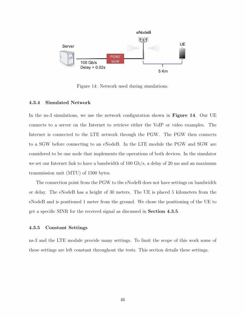
Figure 14: Network used during simulations.
4.3.4 Simulated Network
In the ns-3 simulations, we use the network configuration shown in Figure 14. Our UE
connects to a server on the Internet to retrieve either the VoIP or video examples. The
Internet is connected to the LTE network through the PGW. The PGW then connects
to a SGW before connecting to an eNodeB. In the LTE module the PGW and SGW are
considered to be one node that implements the operations of both devices. In the simulator
we set our Internet link to have a bandwidth of 100 Gb/s, a delay of 20 ms and an maximum
transmission unit (MTU) of 1500 bytes.
The connection point from the PGW to the eNodeB does not have settings on bandwidth
or delay. The eNodeB has a height of 30 meters. The UE is placed 5 kilometers from the
eNodeB and is positioned 1 meter from the ground. We chose the positioning of the UE to
get a specific SINR for the received signal as discussed in Section 4.3.5.
4.3.5 Constant Settings
ns-3 and the LTE module provide many settings. To limit the scope of this work some of
these settings are left constant throughout the tests. This section details these settings.
46
4.3.5.1 Mobility
For our simulations the UE nodes remain stationary throughout the simulation. Mobile
wireless nodes often see variable network conditions due to multipath fading, moving between
cells and entering bad signal locations. In this work we are not looking at situations where
a wireless node moves between cells, we are instead using fading trace files to apply wireless
loss.
4.3.5.2 Distance
The distance from the eNodeB and UE is the same for all of the simulations. In the ns-
3 simulator the distance between the nodes impacts the attenuation on the wireless signal
causing nodes further away to experience a worse SINR. Unless otherwise noted the distance
between the eNodeB and the UE in these simulations is 5Km. The reason for this was to
create a baseline SINR so the UE would report a CQI of 8. This CQI was chosen based on
real measurements described in Appendix B.
4.3.5.3 Available PRBs
As mentioned in Section 2.1.1 an LTE network can support 6 different configurations in
bandwidth ranges providing different number of available PRBs. For all of these simulations
we set the network to have the the maximum frequency range of 20MHz and 100PRBs. This
is the default for the simulator.
4.3.5.4 Basic Radio Environment
ns-3 and the LTE module provide multiple tools for creating the radio environment. This
impacts the SINR the nodes experience. These settings include the power of the transmitters,
background noise, multipath fading models buildings, building materials, interference sources
and fading traces to create a realistic radio environment. In this work, we focus on how LTE
handles loss but we do not look into specific origins of the loss. We use the fading trace file
47
to apply loss as this allows the fine granularity of selecting specific radio frequency ranges
and time frames to apply a poor SINR. We do not examine having interference from any
other wireless transmitters or from having obstructing buildings.
For propagation loss ns-3 has a few options. These simulations use the FriisPropagation-
LossModel since the only factor that impacts SINR is the distance between the eNodeB and
the UE. In these simulations the FriisPropagationLossModel sets the base line SINR that
the fading trace file manipulates.
The settings on transmission powers and noise remain constant throughout the simula-
tions. For the baseline radio environment that the fading trace file manipulates, we created
a setup where the SINR experienced by the UE causes it to send a CQI of 8 to the eNodeB.
The reason for this was that 8 was the average CQI requested from a phone that we took
measurement on for a week as described in Appendix B. Both the eNodeB and UE can have
their transmission powers and noise figures set. The transmission power as its name suggests
sets the amount of power used to transmit. The noise figure is an additional SINR setting
caused by imperfections in the antenna for the device. For this work we keep the noise figure
on both devices set to 0. To set the transmission power we first tried the default settings (30
dBm and 10 dBm for the eNodeB and eNodeB respectively). We then adjusted the position
of the nodes and the transmission power so that both nodes could communicate with one
another with the UE requesting a CQI of 8. Using the default settings for the transmission
power, the UE only requested a CQI of 8 when it was so far away that its own transmissions
could not be heard by the eNodeB. We therefore lowered the transmission power on the
eNodeB and moved the UE closer (to 5Km) so that the UE would request a CQI of 8 and
the eNodeB would be able to hear the transmissions from the UE. The final settings on the
transmission powers was 20dBm for the eNodeB and 10dBm for the UE.
The LTE module also allows for setting the E-UTRA absolute radio frequency channel
number (EARFCN) for both the downlink and the uplink [8]. The EARFCN identify the
carrier frequency used in the uplink and downlink. These were left on their default settings of
48
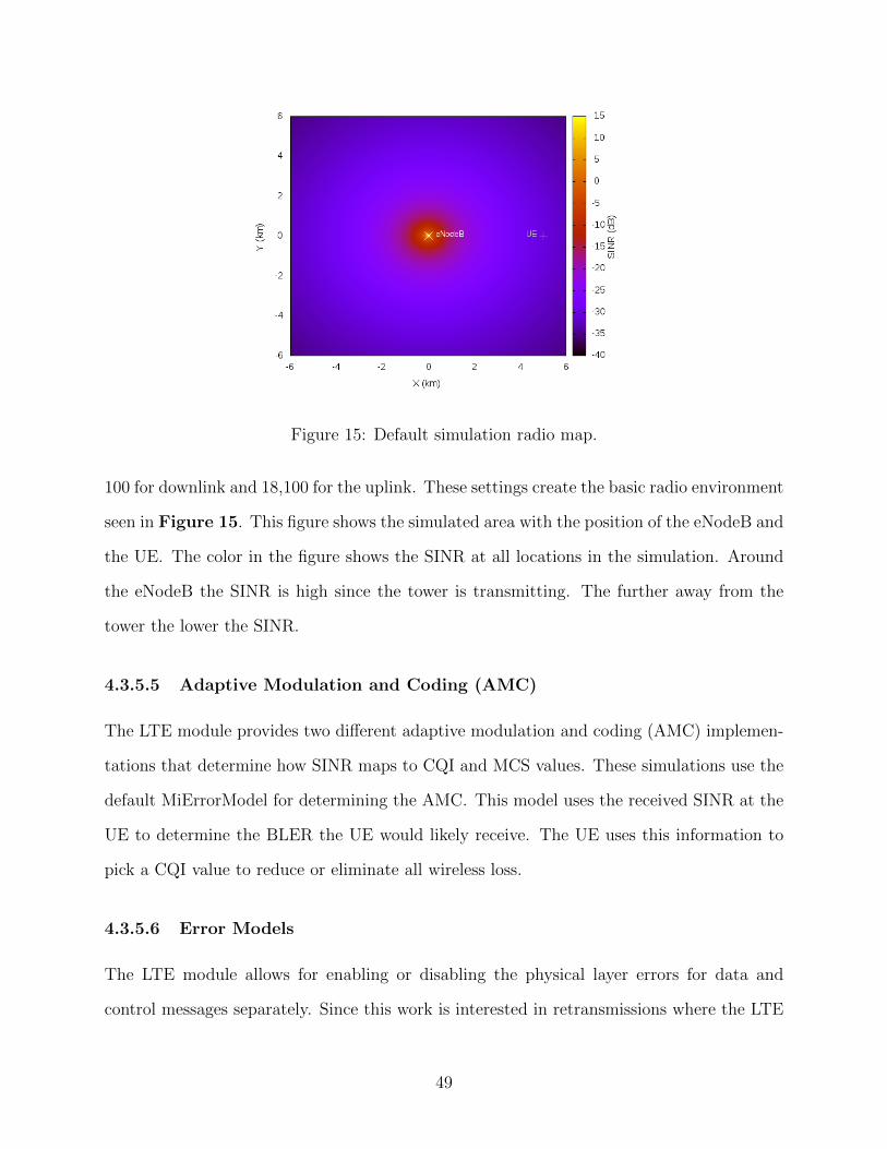
Figure 15: Default simulation radio map.
100 for downlink and 18,100 for the uplink. These settings create the basic radio environment
seen in Figure 15. This figure shows the simulated area with the position of the eNodeB and
the UE. The color in the figure shows the SINR at all locations in the simulation. Around
the eNodeB the SINR is high since the tower is transmitting. The further away from the
tower the lower the SINR.
4.3.5.5 Adaptive Modulation and Coding (AMC)
The LTE module provides two different adaptive modulation and coding (AMC) implemen-
tations that determine how SINR maps to CQI and MCS values. These simulations use the
default MiErrorModel for determining the AMC. This model uses the received SINR at the
UE to determine the BLER the UE would likely receive. The UE uses this information to
pick a CQI value to reduce or eliminate all wireless loss.
4.3.5.6 Error Models
The LTE module allows for enabling or disabling the physical layer errors for data and
control messages separately. Since this work is interested in retransmissions where the LTE
49
control messages work as intended, we set the data error model enabled and the control error
model disabled.
4.3.5.7 Buffers
Both AM and UM use buffers to store data for transmission. However, since AM is supposed
to provide reliable data transmission the ns-3 LTE module implementers set its buffers
without a limit so there should be no dropped data due to buffer overflow. UM on the other
hand does have a setting to set the maximum size of the buffer. Since we are interested in
losses caused by the physical layer and not an overflowing buffer we set the UM buffer, limit
to be 9,999,999 bytes to avoid any dropped data.
4.3.5.8 MAC Scheduler
The LTE module allows setting different MAC schedulers to determine how data is sent and
received from all of the UEs. Since these simulations only have one UE, we use the default
proportional fair MAC scheduler.
4.3.5.9 RLC MaxRetxThreshold
The RLC AM variable maxRetxThreshold determines how many RLC layer retransmissions
are allowed. When a RLC PDU surpasses this retransmission limit, a radio link failure
message is sent to the RRC layer as described in Section 2.1.3. The ns-3 LTE model does
not support sending the radio link failure message to the RRC layer. As a result making
any adjustments to this setting do not have an impact. Since the radio link failure causes
the UE to reset its connection, this work assumes that if a RLC PDU passes its maximum
retransmission threshold then the communication will have failed. The default in the ns-3
simulator for maxRetxThreshold is 5.
50
4.3.5.10 RLC PollBytes and PollPDU
The RLC AM variables PollBytes and PollPDU determine how many PDUs or bytes to send
before requesting a STATUS message from the receiver. For this work we decided to focus
on the timers t-Reordering and t-StatusProhibit so we leave these variables to their default
in the simulator of 1 PDU and 50 bytes.
4.3.5.11 RLC t-PollRetransmit
The RLC AM timer t-PollRetransmit is used by the transmitter to determine how long after
requesting a STATUS message it should wait before sending the poll request again. In this
work we decided to focus on the timers t-Reordering and t-StatusProhibit. This variable is
left with its default setting from the simulator of 100 ms.
4.3.6 Variable Settings
4.3.6.1 Wireless Loss
To adjust the wireless loss experienced by the UE we used a fading trace file. The fading
trace file specifies a SINR value to apply to a specific PRB at a specific TTI. As a result we
can set when and where data can be lost. Normally the fading trace file is generated through
a Matlab script with a set of parameters to create a realistic radio environment10. For these
simulations we are interested in examining how loss and retransmissions impact the higher
level application. We could try generating realistic fading trace files but this means we lose
control over the specific loss instances. Instead we created our own fading traces to control
exactly when and where loss occurs.
For the UE to lose any data the SINR must be low enough that the signal is disrupted
by the noise. LTE is designed to adjust the modulation and coding to keep the BLER to less
than 10% [17]. This means that as the SINR gets lower the UE requests lower CQI values.
10https://www.nsnam.org/docs/models/html/lte-user.html
51
The eNodeB can then respond by choosing a different modulation and coding scheme that
sends less data but with a better chance of it arriving undamaged. While the goal is for
a BLER of 10% the ns-3 LTE module does not automatically add a random error to the
transmission. The simulator uses the SINR combined with the modulation and coding to
determine if a particular transport block would be lost. Since the UE requests a lower CQI
when the SINR worsens, the simulator does not see any transport blocks lost until the SINR
is worse than the eNodeB can compensate. This means that as long as the MCS that the
eNodeB transmits at is above 0 there will be no errors.
When the MCS is 0 there might still be no errors. However once the MCS is at 0 the
eNodeB can no longer compensate so as the SINR continues to worsen there is nothing
that can be done to stop the transport blocks from being corrupted. In real life multiple
interference sources may cause transport blocks to be lost before the UE can request a lower
CQI but for these simulations we are only applying SINR for loss through the fading trace
file.
The values in the fading trace file can lower the SINR at specific times and for specific
PRBs. The UE responds to this by requesting lower CQI values to decrease the throughput
and decrease the chances of lost data. Since we do not have any other sources of wireless
loss in our simulations, we do not lose data until the SINR is low enough that the eNodeB
cannot compensate. We found that applying a SINR of -100dB to a PRB was enough to
cause it to fail on reception.
To create the fading trace files we use two methods. For a first round of tests a simple
uniform probability distribution is used to provide initial insight into how loss impacts the
LTE layers. The majority of the tests however use a Gilbert-Elliot [23] model. The Gilbert-
Elliot model is a common method used to simulate packet loss. This model is depicted in
Figure 16. There are two states to the model. One state is considered good and has low
packet losses while the other state is considered bad with high packet losses. There are
also probabilities that control when to stay in a state or transition to another. The exact
52
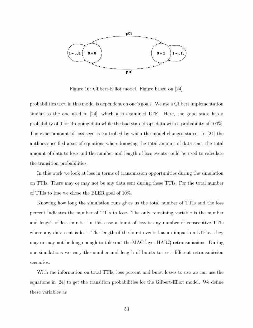
Figure 16: Gilbert-Elliot model. Figure based on [24].
probabilities used in this model is dependent on one’s goals. We use a Gilbert implementation
similar to the one used in [24], which also examined LTE. Here, the good state has a
probability of 0 for dropping data while the bad state drops data with a probability of 100%.
The exact amount of loss seen is controlled by when the model changes states. In [24] the
authors specified a set of equations where knowing the total amount of data sent, the total
amount of data to lose and the number and length of loss events could be used to calculate
the transition probabilities.
In this work we look at loss in terms of transmission opportunities during the simulation
on TTIs. There may or may not be any data sent during these TTIs. For the total number
of TTIs to lose we chose the BLER goal of 10%.
Knowing how long the simulation runs gives us the total number of TTIs and the loss
percent indicates the number of TTIs to lose. The only remaining variable is the number
and length of loss bursts. In this case a burst of loss is any number of consecutive TTIs
where any data sent is lost. The length of the burst events has an impact on LTE as they
may or may not be long enough to take out the MAC layer HARQ retransmissions. During
our simulations we vary the number and length of bursts to test different retransmission
scenarios.
With the information on total TTIs, loss percent and burst losses to use we can use the
equations in [24] to get the transition probabilities for the Gilbert-Elliot model. We define
these variables as
53
• ok - The number of burst losses of length k.
• a - The total number of TTIs.
• d - The total number of lost TTIs.
With these variables we calculate the probability of moving from the good to the bad
state using Equation 5 and the probability of staying in the bad state using Equation 6.
p01 =
∑∞k=1 ok
a(5)
1 − p10 =
∑∞k=1(k − 1) × ok
d− 1(6)
From these equations we get the probabilities of the state changes. However, while these
equations take the number of gaps and gap lengths in as parameters the result from running
the Gilbert-Elliot model will not match up. There is no guarantee that the state change
probabilities will produce the same output as the input parameters. However our goal is to
be able to get the correct overall loss rate. We examine the actual gap lengths versus the
input parameters as we make fading trace files and ensure that the loss rate is correct.
For the initial tests to find the preferred settings of t-Reordering and t-StatusProhibit
we use a loss rate of 10% to match the goal for BLER inside LTE. However once we find
these preferred settings and fix them we create fading trace files with other error rates using
both the Gilbert-Ellilot model bursty loss and comparing this to simple uniform loss rates.
4.3.6.2 RLC Settings
The RLC layer contains a few settings for both AM and UM. These settings impact how
the RLC layer handles retransmissions and how long it waits before declaring data lost. The
specific settings we test are:
54
Table 5: Suggested settings from [5] for some RLC layer timers.
Setting Name Valuest-Reordering 0 ms, 5 ms, 10 ms, 15 ms, 20 ms, 25 ms, 30 ms, 35 ms,
40 ms, 45 ms, 50 ms, 55 ms, 60 ms, 65 ms, 70 ms, 75 ms80 ms, 85 ms, 90 ms, 100 ms, 110 ms, 120 ms, 130 ms140 ms, 150 ms, 160 ms, 170 ms, 180 ms, 190 ms, 200 ms
t-StatusProhibit 0 ms, 5 ms, 10 ms, 15 ms, 20 ms, 25 ms, 30 ms, 35 ms,40 ms, 45 ms, 50 ms, 55 ms, 60 ms, 65 ms, 70 ms, 75 ms80 ms, 85 ms, 90 ms, 95 ms 100 ms, 105 ms, 110 ms,115 ms, 120 ms, 125 ms, 130 ms, 135 ms, 140 ms, 145 ms,150 ms, 155 ms, 160 ms, 165 ms, 170 ms, 175 ms, 180 ms,185 ms, 190 ms, 195 ms, 200 ms, 205 ms, 210 ms, 215 ms,220 ms, 225 ms, 230 ms, 235 ms, 240 ms, 245 ms, 250 ms,300 ms, 350 ms, 400 ms, 450 ms, 500 ms
• t-Reordering - Adjustments to this timer change when the receiving side RLC entity
(AM and UM) detect a lost PDU.
• t-StatusProhibit - Adjustments to this timer change the shortest time between the
receiving side RLC entity sending status messages with ACKs and NACKs.
The specification for the RRC layer defines a set of suggested values for these parameters.
These values are shown in Table 5.
4.3.7 Simulation Time
To determine the amount of time the simulation runs we look at the granularity of events
and the types of applications used. In LTE, data can be transmitted every subframe (1 ms)
so in a matter of seconds the simulation will produce data relating to thousands of possible
transmissions and retransmissions. When examining retransmissions at the lower layer we
can run experiments for a few seconds. When examining the performance at the application
layer we need to run the simulation for longer.
The application should run long enough in the simulation to overcome any natural varia-
tion in its nature. For instance in TCP there is the slow start phase that starts the congestion
window small. This causes an initial low bandwidth for the application using TCP (in this
55
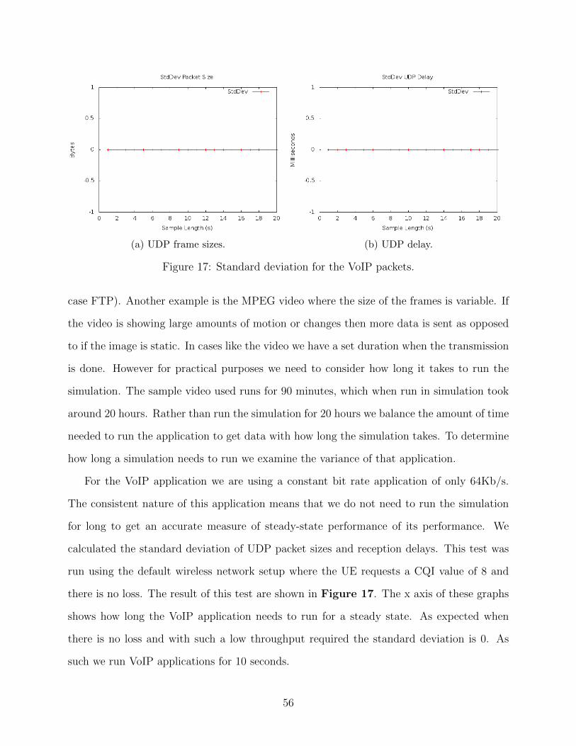
(a) UDP frame sizes. (b) UDP delay.
Figure 17: Standard deviation for the VoIP packets.
case FTP). Another example is the MPEG video where the size of the frames is variable. If
the video is showing large amounts of motion or changes then more data is sent as opposed
to if the image is static. In cases like the video we have a set duration when the transmission
is done. However for practical purposes we need to consider how long it takes to run the
simulation. The sample video used runs for 90 minutes, which when run in simulation took
around 20 hours. Rather than run the simulation for 20 hours we balance the amount of time
needed to run the application to get data with how long the simulation takes. To determine
how long a simulation needs to run we examine the variance of that application.
For the VoIP application we are using a constant bit rate application of only 64Kb/s.
The consistent nature of this application means that we do not need to run the simulation
for long to get an accurate measure of steady-state performance of its performance. We
calculated the standard deviation of UDP packet sizes and reception delays. This test was
run using the default wireless network setup where the UE requests a CQI value of 8 and
there is no loss. The result of this test are shown in Figure 17. The x axis of these graphs
shows how long the VoIP application needs to run for a steady state. As expected when
there is no loss and with such a low throughput required the standard deviation is 0. As
such we run VoIP applications for 10 seconds.
56

(a) Full TCP trace. (b) TCP trace after initial startup.
Figure 18: Standard deviation for the MPEG application.
For the FTP application the TCP throughput is of interest. When sending a file the
delay is not as much of a concern as receiving the file properly so we are not as concerned
with the delay of the TCP packets. To determine how long the FTP application should
run we examine the standard deviation of the throughput as shown in Figure 18. When
examining throughput we look at the data sent over time. For this example for each second
of simulation time we add up all of the packets received in that second to get the number of
bits received in that second. We do not average the throughput over more than one second.
The initial variation in the application comes from the slow start phase of the TCP
congestion window. Once the TCP congestion window fills the maximum bandwidth the
connection allows the flow of TCP ACKs to throttle the sending rate. In Figure 18a
the standard deviation on the throughput initially varies within 2 Mb/s before eventually
dropping below 0.5 Mb/s. By starting the throughput analysis one second after the FTP
application starts the the standard deviation becomes much more stable as seen in Figure
18b. Since the standard deviation remains stable we can run the FTP simulation for only
a few seconds as long as we note the slow start discrepancy. The FTP simulations will run
for 11 seconds (1 second of slow start and 10 seconds of normal operation when there is no
loss).
57
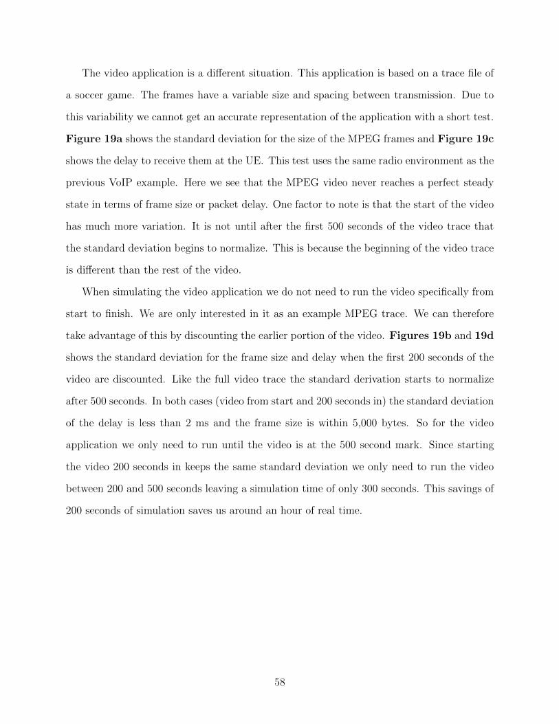
The video application is a different situation. This application is based on a trace file of
a soccer game. The frames have a variable size and spacing between transmission. Due to
this variability we cannot get an accurate representation of the application with a short test.
Figure 19a shows the standard deviation for the size of the MPEG frames and Figure 19c
shows the delay to receive them at the UE. This test uses the same radio environment as the
previous VoIP example. Here we see that the MPEG video never reaches a perfect steady
state in terms of frame size or packet delay. One factor to note is that the start of the video
has much more variation. It is not until after the first 500 seconds of the video trace that
the standard deviation begins to normalize. This is because the beginning of the video trace
is different than the rest of the video.
When simulating the video application we do not need to run the video specifically from
start to finish. We are only interested in it as an example MPEG trace. We can therefore
take advantage of this by discounting the earlier portion of the video. Figures 19b and 19d
shows the standard deviation for the frame size and delay when the first 200 seconds of the
video are discounted. Like the full video trace the standard derivation starts to normalize
after 500 seconds. In both cases (video from start and 200 seconds in) the standard deviation
of the delay is less than 2 ms and the frame size is within 5,000 bytes. So for the video
application we only need to run until the video is at the 500 second mark. Since starting
the video 200 seconds in keeps the same standard deviation we only need to run the video
between 200 and 500 seconds leaving a simulation time of only 300 seconds. This savings of
200 seconds of simulation saves us around an hour of real time.
58
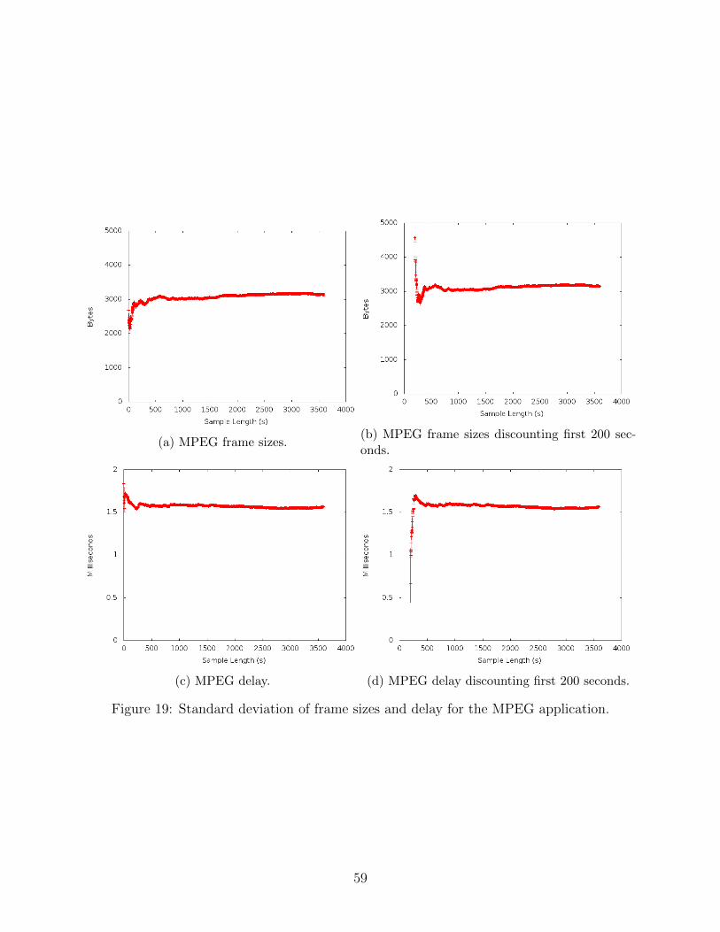
(a) MPEG frame sizes.(b) MPEG frame sizes discounting first 200 sec-onds.
(c) MPEG delay. (d) MPEG delay discounting first 200 seconds.
Figure 19: Standard deviation of frame sizes and delay for the MPEG application.
59
5 Results
This section looks at the results of running simulations in ns-3. Section 5.1 examine the
changes made to support NACKs in STATUS messages. Section 5.2 is the baseline test
for all applications with no wireless loss. Section 5.2.2 covers the basics of how wireless
loss impacts the applications. The results of the application simulations for VoIP, FTP and
MPEG are provided in Sections 5.3, 5.4 and 5.5 respectively.
5.1 ns-3 LTE Additions
5.1.1 Adding NACKs to Status PDUs
As mentioned in Section 4.2 we needed to modify the LTE simulation module to support the
use of NACKs in RLC AM. The first of these changes was to add support for serializing and
de-serializing the NACK SNs in the RLC AM status PDU. We submitted an initial patch to
the LTE module developers who wrote a test case to validate the result. This exposed some
flaws in the initial patch, which we corrected. The final version of this patch passed the test
case. The test case created by the developers simply input information to place in the status
PDU and confirmed that the resulting bytes in the header created the correct number.
5.1.2 Detecting Sequence Numbers to NACK
The other additions to the simulator identified which PDUs had not been received and
making the correct NACK requests to retrieve them. Once again the developers of the
LTE module created a test case to validate this work. The test case set the loss rate and
checked that the receiving RLC AM entity sent back the correct NACKs to retrieve all of
the missing PDUs. There was no limit to the number of retransmissions. After multiple
rounds of working with the developers and others on the discussion forum, finding bugs and
suggesting fixes we finally got all of these tests to pass.
60
Figure 20 shows four different loss rates during the test case. The test is setup to send
1,000 RRC layer PDUs from one eNodeB to an UE. The test passes if all 1,000 PDUs make
it. Since the PDUs are from the higher RRC layer the RLC layer may deliver one RRC
PDU per RLC PDU or one RLC PDU may contain multiple RRC PDUs. In Figure 20a
and Figure 20b the loss rate of 0% and 25% respectively produces very similar graphs. In
Figure 20a the lower bound on the receiving window VR(R) is obstructed by VR(H), the
highest seen SN. In Figure 20b you can see VR(R) more as there is some loss of packets.
Figures 20c and 20d show more diversity due to the higher loss rates of 75% and 95%
respectively. VR(H) stays higher than VR(R) most of the time due to so many lost packets.
Fewer total RLC layer PDUs were received. As PDUs were lost the RLC layer started to
pack more RRC PDUs into the RLC PDUs. This is because the loss rate set in the simulation
does not take into account the radio physical layer. So the total amount of data that can be
sent during each transmission opportunity is large. As PDUs are lost they are moved into
the retransmission buffer. As the buffer fills the transmission opportunities have more data
available to pack into the RLC PDUs. At the end of Figures 20c and 20d the lower bound
on the receive window finally matches the highest RLC PDU sequence number received.
5.2 Baseline
5.2.1 No Loss
The first simulation set a baseline for the VoIP and video data. This simulation had no loss
and checks how the VoIP and video examples work in both UM and AM. The important
results in this section is the delay experienced by the applications without any retransmissions
or adjustments to other RLC settings. Future tests compare against the baseline to see how
the retransmissions impact both the amount and variability of delay.
61
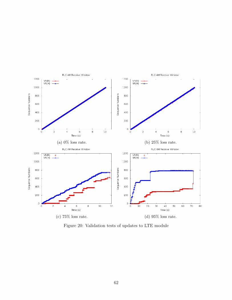
(a) 0% loss rate. (b) 25% loss rate.
(c) 75% loss rate. (d) 95% loss rate.
Figure 20: Validation tests of updates to LTE module
62
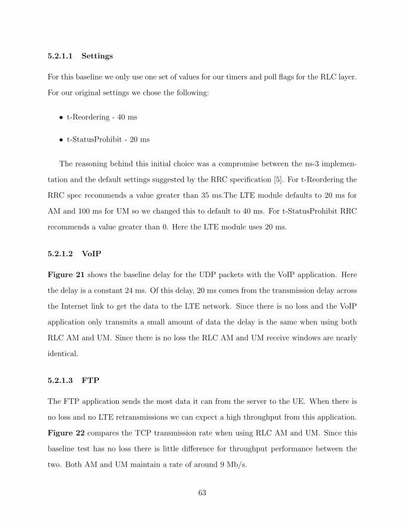
5.2.1.1 Settings
For this baseline we only use one set of values for our timers and poll flags for the RLC layer.
For our original settings we chose the following:
• t-Reordering - 40 ms
• t-StatusProhibit - 20 ms
The reasoning behind this initial choice was a compromise between the ns-3 implemen-
tation and the default settings suggested by the RRC specification [5]. For t-Reordering the
RRC spec recommends a value greater than 35 ms.The LTE module defaults to 20 ms for
AM and 100 ms for UM so we changed this to default to 40 ms. For t-StatusProhibit RRC
recommends a value greater than 0. Here the LTE module uses 20 ms.
5.2.1.2 VoIP
Figure 21 shows the baseline delay for the UDP packets with the VoIP application. Here
the delay is a constant 24 ms. Of this delay, 20 ms comes from the transmission delay across
the Internet link to get the data to the LTE network. Since there is no loss and the VoIP
application only transmits a small amount of data the delay is the same when using both
RLC AM and UM. Since there is no loss the RLC AM and UM receive windows are nearly
identical.
5.2.1.3 FTP
The FTP application sends the most data it can from the server to the UE. When there is
no loss and no LTE retransmissions we can expect a high throughput from this application.
Figure 22 compares the TCP transmission rate when using RLC AM and UM. Since this
baseline test has no loss there is little difference for throughput performance between the
two. Both AM and UM maintain a rate of around 9 Mb/s.
63
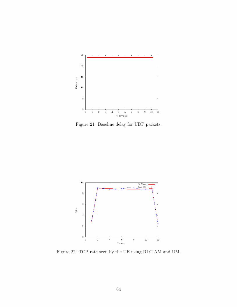
Figure 21: Baseline delay for UDP packets.
Figure 22: TCP rate seen by the UE using RLC AM and UM.
64
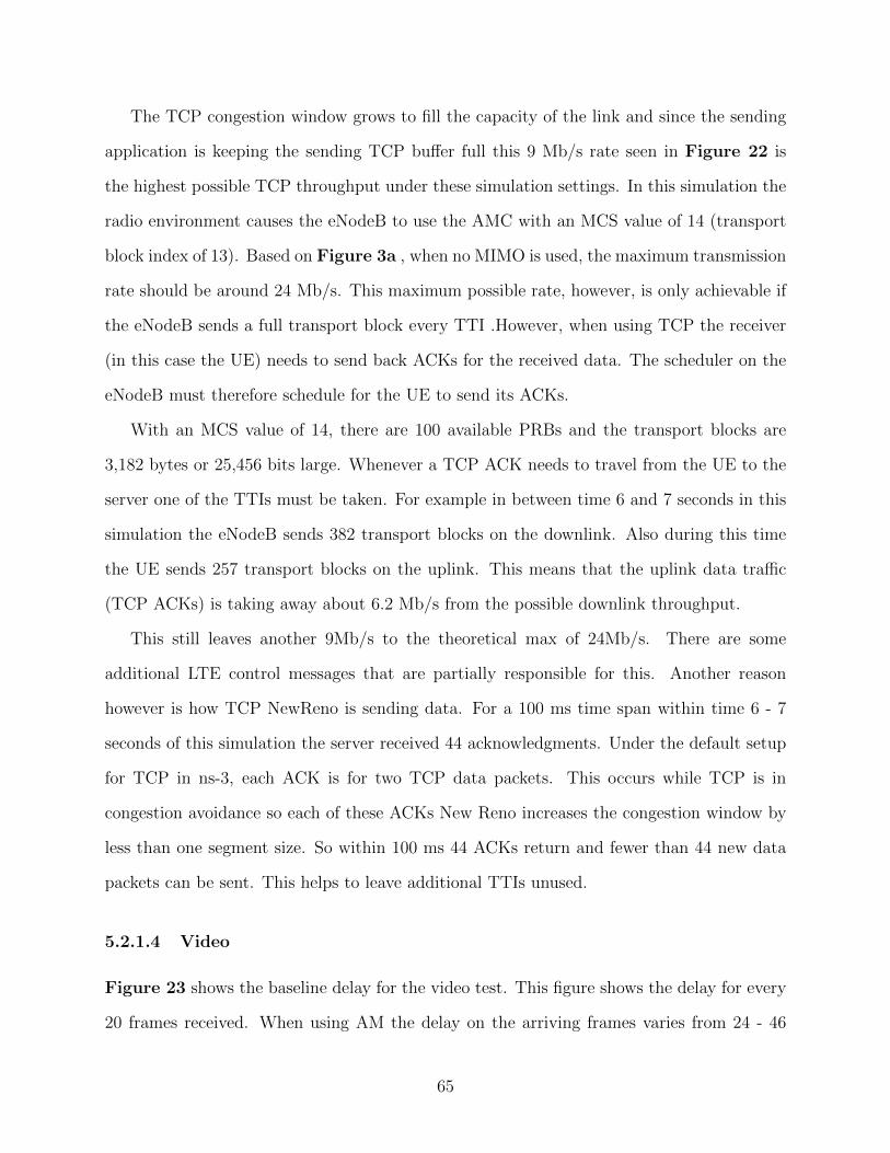
The TCP congestion window grows to fill the capacity of the link and since the sending
application is keeping the sending TCP buffer full this 9 Mb/s rate seen in Figure 22 is
the highest possible TCP throughput under these simulation settings. In this simulation the
radio environment causes the eNodeB to use the AMC with an MCS value of 14 (transport
block index of 13). Based on Figure 3a , when no MIMO is used, the maximum transmission
rate should be around 24 Mb/s. This maximum possible rate, however, is only achievable if
the eNodeB sends a full transport block every TTI .However, when using TCP the receiver
(in this case the UE) needs to send back ACKs for the received data. The scheduler on the
eNodeB must therefore schedule for the UE to send its ACKs.
With an MCS value of 14, there are 100 available PRBs and the transport blocks are
3,182 bytes or 25,456 bits large. Whenever a TCP ACK needs to travel from the UE to the
server one of the TTIs must be taken. For example in between time 6 and 7 seconds in this
simulation the eNodeB sends 382 transport blocks on the downlink. Also during this time
the UE sends 257 transport blocks on the uplink. This means that the uplink data traffic
(TCP ACKs) is taking away about 6.2 Mb/s from the possible downlink throughput.
This still leaves another 9Mb/s to the theoretical max of 24Mb/s. There are some
additional LTE control messages that are partially responsible for this. Another reason
however is how TCP NewReno is sending data. For a 100 ms time span within time 6 - 7
seconds of this simulation the server received 44 acknowledgments. Under the default setup
for TCP in ns-3, each ACK is for two TCP data packets. This occurs while TCP is in
congestion avoidance so each of these ACKs New Reno increases the congestion window by
less than one segment size. So within 100 ms 44 ACKs return and fewer than 44 new data
packets can be sent. This helps to leave additional TTIs unused.
5.2.1.4 Video
Figure 23 shows the baseline delay for the video test. This figure shows the delay for every
20 frames received. When using AM the delay on the arriving frames varies from 24 - 46
65
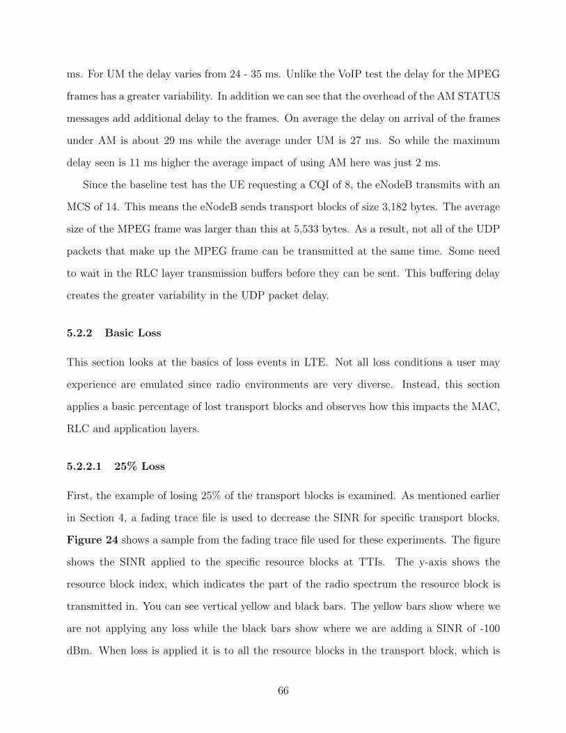
ms. For UM the delay varies from 24 - 35 ms. Unlike the VoIP test the delay for the MPEG
frames has a greater variability. In addition we can see that the overhead of the AM STATUS
messages add additional delay to the frames. On average the delay on arrival of the frames
under AM is about 29 ms while the average under UM is 27 ms. So while the maximum
delay seen is 11 ms higher the average impact of using AM here was just 2 ms.
Since the baseline test has the UE requesting a CQI of 8, the eNodeB transmits with an
MCS of 14. This means the eNodeB sends transport blocks of size 3,182 bytes. The average
size of the MPEG frame was larger than this at 5,533 bytes. As a result, not all of the UDP
packets that make up the MPEG frame can be transmitted at the same time. Some need
to wait in the RLC layer transmission buffers before they can be sent. This buffering delay
creates the greater variability in the UDP packet delay.
5.2.2 Basic Loss
This section looks at the basics of loss events in LTE. Not all loss conditions a user may
experience are emulated since radio environments are very diverse. Instead, this section
applies a basic percentage of lost transport blocks and observes how this impacts the MAC,
RLC and application layers.
5.2.2.1 25% Loss
First, the example of losing 25% of the transport blocks is examined. As mentioned earlier
in Section 4, a fading trace file is used to decrease the SINR for specific transport blocks.
Figure 24 shows a sample from the fading trace file used for these experiments. The figure
shows the SINR applied to the specific resource blocks at TTIs. The y-axis shows the
resource block index, which indicates the part of the radio spectrum the resource block is
transmitted in. You can see vertical yellow and black bars. The yellow bars show where we
are not applying any loss while the black bars show where we are adding a SINR of -100
dBm. When loss is applied it is to all the resource blocks in the transport block, which is
66
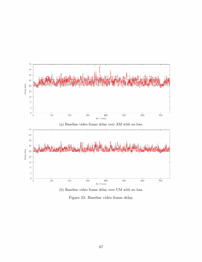
(a) Baseline video frame delay over AM with no loss.
(b) Baseline video frame delay over UM with no loss.
Figure 23: Baseline video frame delay.
67
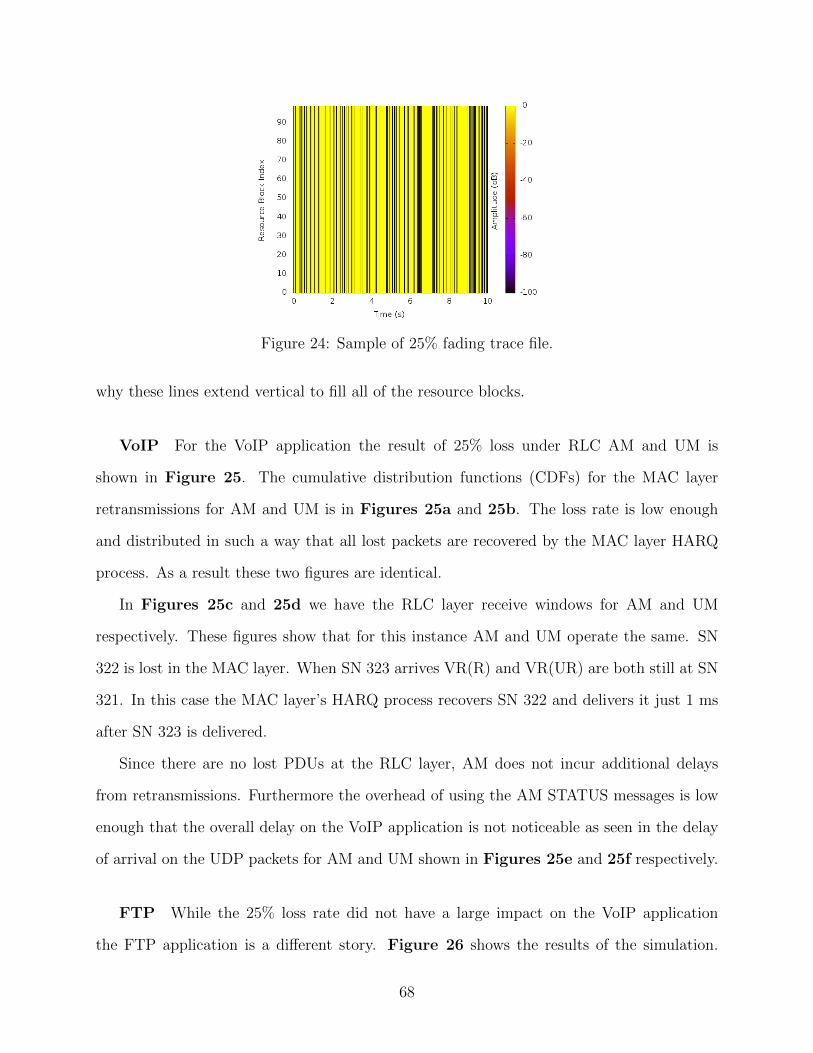
Figure 24: Sample of 25% fading trace file.
why these lines extend vertical to fill all of the resource blocks.
VoIP For the VoIP application the result of 25% loss under RLC AM and UM is
shown in Figure 25. The cumulative distribution functions (CDFs) for the MAC layer
retransmissions for AM and UM is in Figures 25a and 25b. The loss rate is low enough
and distributed in such a way that all lost packets are recovered by the MAC layer HARQ
process. As a result these two figures are identical.
In Figures 25c and 25d we have the RLC layer receive windows for AM and UM
respectively. These figures show that for this instance AM and UM operate the same. SN
322 is lost in the MAC layer. When SN 323 arrives VR(R) and VR(UR) are both still at SN
321. In this case the MAC layer’s HARQ process recovers SN 322 and delivers it just 1 ms
after SN 323 is delivered.
Since there are no lost PDUs at the RLC layer, AM does not incur additional delays
from retransmissions. Furthermore the overhead of using the AM STATUS messages is low
enough that the overall delay on the VoIP application is not noticeable as seen in the delay
of arrival on the UDP packets for AM and UM shown in Figures 25e and 25f respectively.
FTP While the 25% loss rate did not have a large impact on the VoIP application
the FTP application is a different story. Figure 26 shows the results of the simulation.
68
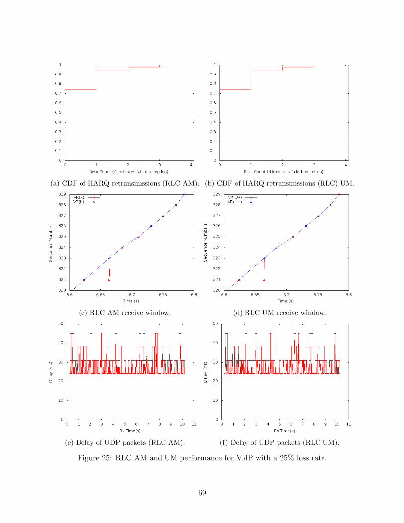
(a) CDF of HARQ retransmissions (RLC AM). (b) CDF of HARQ retransmissions (RLC) UM.
(c) RLC AM receive window. (d) RLC UM receive window.
(e) Delay of UDP packets (RLC AM). (f) Delay of UDP packets (RLC UM).
Figure 25: RLC AM and UM performance for VoIP with a 25% loss rate.
69
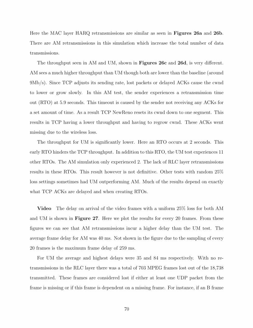
Here the MAC layer HARQ retransmissions are similar as seen in Figures 26a and 26b.
There are AM retransmissions in this simulation which increase the total number of data
transmissions.
The throughput seen in AM and UM, shown in Figures 26c and 26d, is very different.
AM sees a much higher throughput than UM though both are lower than the baseline (around
9Mb/s). Since TCP adjusts its sending rate, lost packets or delayed ACKs cause the cwnd
to lower or grow slowly. In this AM test, the sender experiences a retransmission time
out (RTO) at 5.9 seconds. This timeout is caused by the sender not receiving any ACKs for
a set amount of time. As a result TCP NewReno resets its cwnd down to one segment. This
results in TCP having a lower throughput and having to regrow cwnd. These ACKs went
missing due to the wireless loss.
The throughput for UM is significantly lower. Here an RTO occurs at 2 seconds. This
early RTO hinders the TCP throughput. In addition to this RTO, the UM test experiences 11
other RTOs. The AM simulation only experienced 2. The lack of RLC layer retransmissions
results in these RTOs. This result however is not definitive. Other tests with random 25%
loss settings sometimes had UM outperforming AM. Much of the results depend on exactly
what TCP ACKs are delayed and when creating RTOs.
Video The delay on arrival of the video frames with a uniform 25% loss for both AM
and UM is shown in Figure 27. Here we plot the results for every 20 frames. From these
figures we can see that AM retransmissions incur a higher delay than the UM test. The
average frame delay for AM was 40 ms. Not shown in the figure due to the sampling of every
20 frames is the maximum frame delay of 259 ms.
For UM the average and highest delays were 35 and 84 ms respectively. With no re-
transmissions in the RLC layer there was a total of 703 MPEG frames lost out of the 18,738
transmitted. These frames are considered lost if either at least one UDP packet from the
frame is missing or if this frame is dependent on a missing frame. For instance, if an B frame
70
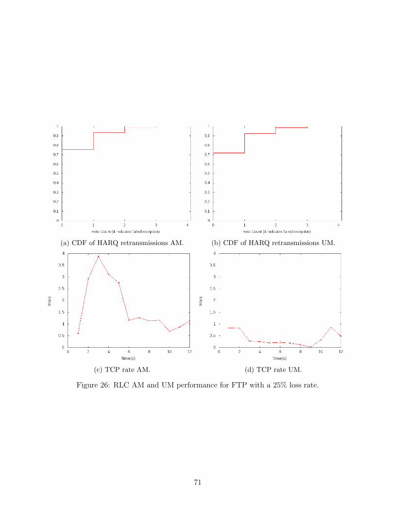
(a) CDF of HARQ retransmissions AM. (b) CDF of HARQ retransmissions UM.
(c) TCP rate AM. (d) TCP rate UM.
Figure 26: RLC AM and UM performance for FTP with a 25% loss rate.
71
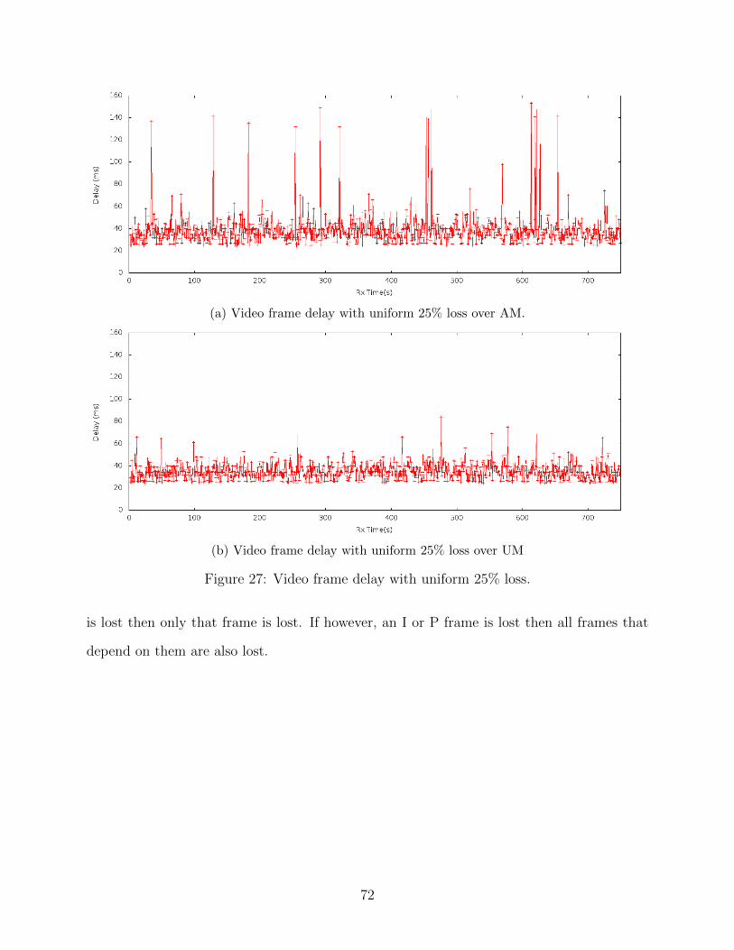
(a) Video frame delay with uniform 25% loss over AM.
(b) Video frame delay with uniform 25% loss over UM
Figure 27: Video frame delay with uniform 25% loss.
is lost then only that frame is lost. If however, an I or P frame is lost then all frames that
depend on them are also lost.
72

5.3 VoIP Simulations
This section investigates at how bursty loss events combined with modification to RLC layer
settings impact the VoIP application. First the t-Reordering and t-StatusProhibit timers are
adjusted to find settings that provide better performance for VoIP. Then with these timers
fixed, the loss rate of the wireless link is adjusted to find if VoIP works better under AM or
UM.
5.3.1 VoIP with varied RLC settings
To setup the fading trace file we select a loss rate of 10%. Additionally, we need some example
gap lengths for Equations 5 and 6. These equations set the transition probabilities when
the gap lengths are known. We need the transition probabilities to generate our gap lengths.
We first select a set of input gap lengths to generate the transition probabilities and then
use the Gilbert model to generate the wireless gaps to use in the simulation. For the input
gap lengths we randomly select gaps between 1 - 30 ms inclusive and then randomly select
the number of those gaps to match the loss percentage. We chose these gap lengths due to
the RTT for the MAC layer HARQ process. We want to be sure that the gap lengths can
be large enough to encompass the 3 maximum retransmissions. With these retransmissions
taking 7 ms in the simulator, a gap length of 21 would be sufficient. We rounded this up to
30 to account for more input gap lengths. The output of these equations gave us the state
change probabilities. While in the good state there is a 0.633% probability of transitioning
to the bad state. When in the bad state there is a 6.255% probability of transitioning to the
good state.
The result of this was a fading trace file that had 9.96% total loss of TTIs. The CDF
in Figure 28 comparing a uniform 10% loss, the input gap lengths to the model and the
resulting gap length used to create the fading trace file.
While our simulation shows the delay of delivering UDP packets, this is not representative
73
Figure 28: CDF of loss gap lengths.
of a full VoIP conversation. We used a simple simulation where a server sent the UDP packets
into the LTE E-UTRA network. In a real situation there would be another VoIP client
sending data into the core network that would then be directed to the LTE network. To
account for the core latency of getting the UDP packets to the LTE network, we add a fixed
delay to all of the packets. We use latency statistics collected in the Verizon network available
from [40] to try two call scenarios. One call represents trans Atlantic and the other trans
Pacific. These statistics represent the latency on Internet control message protocol (ICMP)
packets that traveled through core networks to span different network ranges. This data
from Verizon is for on March 2014. As the statistics shown in [40] are likely to be updated
we have recorded them in Table 6. When calculating the MOS and delays for these tests we
add the delays reported by Verizon to account for the core network delays. The simulations
have a server that sends data into the LTE network over a link with a delay of 20 ms. This
delay would be a part of the Verizon core network delay so 20 ms is also subtracted from
the Verizon core network delays to take this into account.
To calculate the MOS we could look at the entire simulation and get the average. How-
ever, in a conversation, bursts of bad errors could cause the user to perceive the call as bad
quality even when the average for the entire conversation is good. If we take any arbitrarily
small unit of time to calculate the MOS, we can see results for only a few packets, which may
74
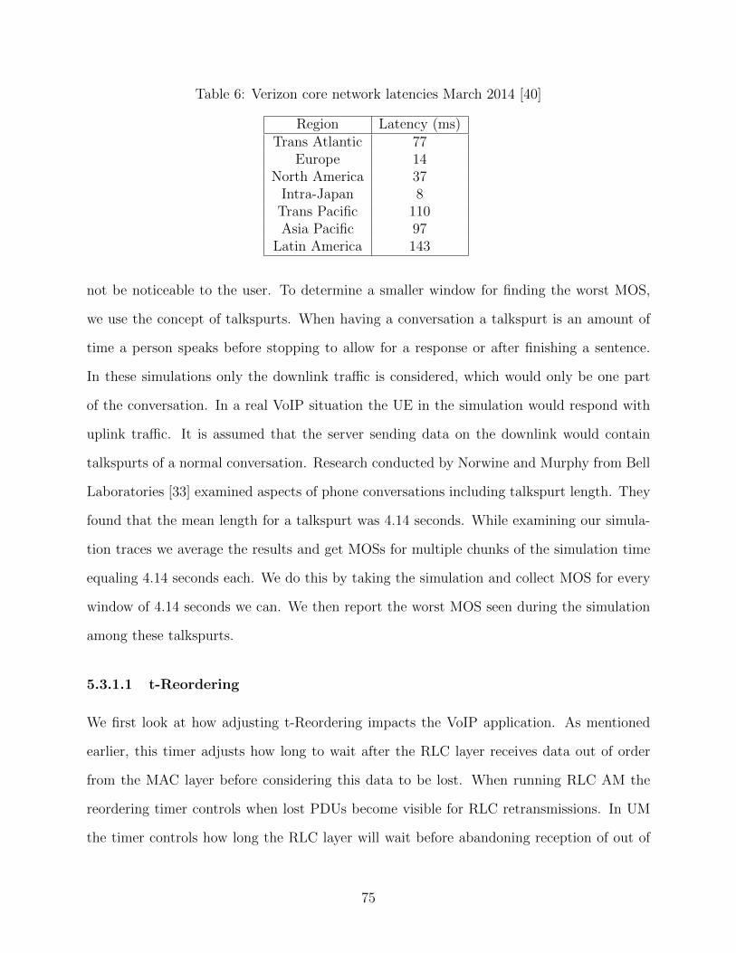
Table 6: Verizon core network latencies March 2014 [40]
Region Latency (ms)Trans Atlantic 77
Europe 14North America 37
Intra-Japan 8Trans Pacific 110Asia Pacific 97
Latin America 143
not be noticeable to the user. To determine a smaller window for finding the worst MOS,
we use the concept of talkspurts. When having a conversation a talkspurt is an amount of
time a person speaks before stopping to allow for a response or after finishing a sentence.
In these simulations only the downlink traffic is considered, which would only be one part
of the conversation. In a real VoIP situation the UE in the simulation would respond with
uplink traffic. It is assumed that the server sending data on the downlink would contain
talkspurts of a normal conversation. Research conducted by Norwine and Murphy from Bell
Laboratories [33] examined aspects of phone conversations including talkspurt length. They
found that the mean length for a talkspurt was 4.14 seconds. While examining our simula-
tion traces we average the results and get MOSs for multiple chunks of the simulation time
equaling 4.14 seconds each. We do this by taking the simulation and collect MOS for every
window of 4.14 seconds we can. We then report the worst MOS seen during the simulation
among these talkspurts.
5.3.1.1 t-Reordering
We first look at how adjusting t-Reordering impacts the VoIP application. As mentioned
earlier, this timer adjusts how long to wait after the RLC layer receives data out of order
from the MAC layer before considering this data to be lost. When running RLC AM the
reordering timer controls when lost PDUs become visible for RLC retransmissions. In UM
the timer controls how long the RLC layer will wait before abandoning reception of out of
75
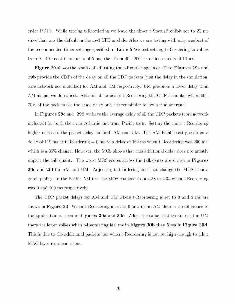
order PDUs. While testing t-Reordering we leave the timer t-StatusProhibit set to 20 ms
since that was the default in the ns-3 LTE module. Also we are testing with only a subset of
the recommended timer settings specified in Table 5 We test setting t-Reordering to values
from 0 - 40 ms at increments of 5 ms, then from 40 - 200 ms at increments of 10 ms.
Figure 29 shows the results of adjusting the t-Reordering timer. First Figures 29a and
29b provide the CDFs of the delay on all the UDP packets (just the delay in the simulation,
core network not included) for AM and UM respectively. UM produces a lower delay than
AM as one would expect. Also for all values of t-Reordering the CDF is similar where 60 -
70% of the packets see the same delay and the remainder follow a similar trend.
In Figures 29c and 29d we have the average delay of all the UDP packets (core network
included) for both the trans Atlantic and trans Pacific tests. Setting the timer t-Reordering
higher increases the packet delay for both AM and UM. The AM Pacific test goes from a
delay of 119 ms at t-Reordering = 0 ms to a delay of 162 ms when t-Reordering was 200 ms,
which is a 36% change. However, the MOS shows that this additional delay does not greatly
impact the call quality. The worst MOS scores across the talkspurts are shown in Figures
29e and 29f for AM and UM. Adjusting t-Reordering does not change the MOS from a
good quality. In the Pacific AM test the MOS changed from 4.38 to 4.34 when t-Reordering
was 0 and 200 ms respectively.
The UDP packet delays for AM and UM where t-Reordering is set to 0 and 5 ms are
shown in Figure 30. When t-Reordering is set to 0 or 5 ms in AM there is no difference to
the application as seen in Figures 30a and 30c. When the same settings are used in UM
there are fewer spikes when t-Reordering is 0 ms in Figure 30b than 5 ms in Figure 30d.
This is due to the additional packets lost when t-Reordering is not set high enough to allow
MAC layer retransmissions.
76
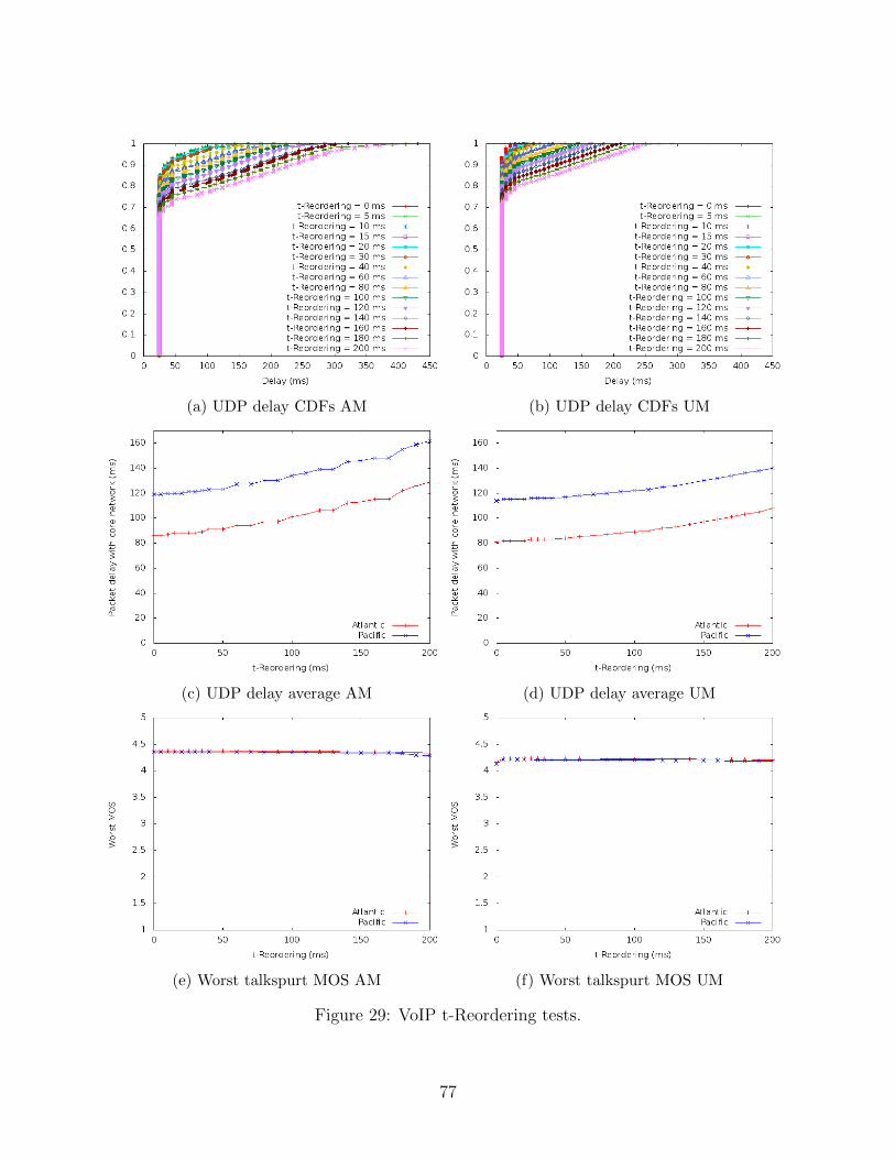
(a) UDP delay CDFs AM (b) UDP delay CDFs UM
(c) UDP delay average AM (d) UDP delay average UM
(e) Worst talkspurt MOS AM (f) Worst talkspurt MOS UM
Figure 29: VoIP t-Reordering tests.
77
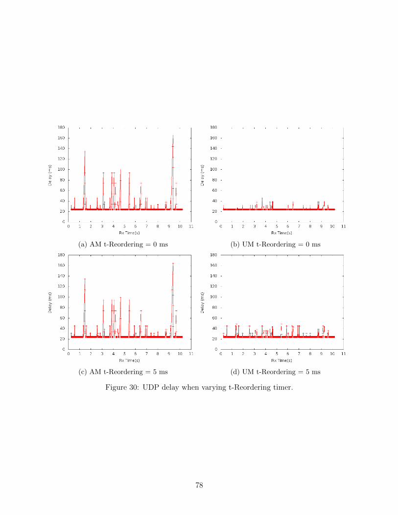
(a) AM t-Reordering = 0 ms (b) UM t-Reordering = 0 ms
(c) AM t-Reordering = 5 ms (d) UM t-Reordering = 5 ms
Figure 30: UDP delay when varying t-Reordering timer.
78
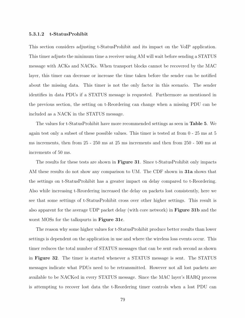
5.3.1.2 t-StatusProhibit
This section considers adjusting t-StatusProhibit and its impact on the VoIP application.
This timer adjusts the minimum time a receiver using AM will wait before sending a STATUS
message with ACKs and NACKs. When transport blocks cannot be recovered by the MAC
layer, this timer can decrease or increase the time taken before the sender can be notified
about the missing data. This timer is not the only factor in this scenario. The sender
identifies in data PDUs if a STATUS message is requested. Furthermore as mentioned in
the previous section, the setting on t-Reordering can change when a missing PDU can be
included as a NACK in the STATUS message.
The values for t-StatusProhibit have more recommended settings as seen in Table 5. We
again test only a subset of these possible values. This timer is tested at from 0 - 25 ms at 5
ms increments, then from 25 - 250 ms at 25 ms increments and then from 250 - 500 ms at
increments of 50 ms.
The results for these tests are shown in Figure 31. Since t-StatusProhibit only impacts
AM these results do not show any comparison to UM. The CDF shown in 31a shows that
the settings on t-StatusProhibit has a greater impact on delay compared to t-Reordering.
Also while increasing t-Reordering increased the delay on packets lost consistently, here we
see that some settings of t-StatusProhibit cross over other higher settings. This result is
also apparent for the average UDP packet delay (with core network) in Figure 31b and the
worst MOSs for the talkspurts in Figure 31c.
The reason why some higher values for t-StatusProhibit produce better results than lower
settings is dependent on the application in use and where the wireless loss events occur. This
timer reduces the total number of STATUS messages that can be sent each second as shown
in Figure 32. The timer is started whenever a STATUS message is sent. The STATUS
messages indicate what PDUs need to be retransmitted. However not all lost packets are
available to be NACKed in every STATUS message. Since the MAC layer’s HARQ process
is attempting to recover lost data the t-Reordering timer controls when a lost PDU can
79

(a) UDP delay CDF for t-StatusProhibit.
(b) UDP delay average AM
(c) Worst talkspurt MOS AM
Figure 31: VoIP t-StatusProhibit tests.
80
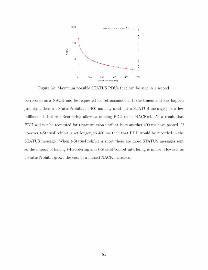
Figure 32: Maximum possible STATUS PDUs that can be sent in 1 second.
be recored as a NACK and be requested for retransmission. If the timers and loss happen
just right then a t-StatusProhibit of 400 ms may send out a STATUS message just a few
milliseconds before t-Reordering allows a missing PDU to be NACKed. As a result that
PDU will not be requested for retransmission until at least another 400 ms have passed. If
however t-StatusProhibit is set longer, to 450 ms then that PDU would be recorded in the
STATUS message. When t-StatusProhibit is short there are more STATUS messages sent
so the impact of having t-Reordering and t-StatusProhibit interfering is minor. However as
t-StatusProhibit grows the cost of a missed NACK increases.
81

5.3.2 VoIP with AM vs UM with varied loss
We next want to fix both t-Reordering and t-StatusProhibit and adjust the amount of
wireless loss using the Gilbert-Elliot model. From the previous tests we know that adjusting
t-Reordering has little impact while having a large t-StatusProhibit increases the cost of
missing NACKs. We set t-Reordering to 30 ms. Because we do not want to risk loosing
any PDUs that could be recovered by the MAC layer. Since the timer is not started until a
PDU with a higher SN is received and LTE can send data every millisecond we only need to
worry about the three retransmissions. With a HARQ RTT of 8 ms we need to make sure
the timer is at least 24 ms. We chose 30 ms to allow some room for starting the timer.
We set the value of t-StatusProhibit to 50 ms. From the previous tests in Figure 31b
and 31c we can see that a setting of 50 ms does not experience the same performance
impacts as higher values. Also Figure 32 indicates that the potential cost of having very
low values could consume many TTIs leaving few for user data.
Next the Gilbert-Ellilot model was used to create fading trace files for loss rates of 5%,
10%, 15%, 20%, 25%, 30%, 35%, 40%, 45% and 50%. For loss rates 5 - 35%, we can generate
the loss gap lengths using our original method where we first randomly select a set of gap
lengths from 0 to 30 to find the state transition probabilities that are then used to run the
Gilbert model to generate the actual fading loss trace. However for loss rates 40 - 50% these
gap lengths proved too small. The resulting state transition probabilities kept producing
fading trace files with total loss percentages less than their targets. So for loss rates 40 -
50% we randomly select gap lengths up to 100 as input. This then produced state transition
probabilities for the Gilbert model which resulted in fading trace files that met the loss goals.
The results of these simulations are shown in Figure 33 for the Gilbert loss model where
our input gap lengths are up to size 30 while Figure 34 shows the results for higher loss
rate where we increased the gap lengths on the input data up to 100. Here for the Atlantic
(left) and Pacific (right) tests we see that at low loss rates the performance of AM and UM
are similar. However as the loss rates increase the extra delay in using AM out weighs the
82
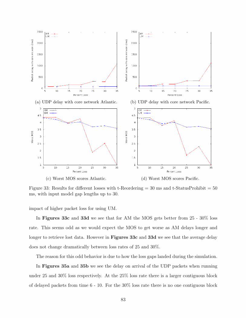
(a) UDP delay with core network Atlantic. (b) UDP delay with core network Pacific.
(c) Worst MOS scores Atlantic. (d) Worst MOS scores Pacific.
Figure 33: Results for different losses with t-Reordering = 30 ms and t-StatusProhibit = 50ms, with input model gap lengths up to 30.
impact of higher packet loss for using UM.
In Figures 33c and 33d we see that for AM the MOS gets better from 25 - 30% loss
rate. This seems odd as we would expect the MOS to get worse as AM delays longer and
longer to retrieve lost data. However in Figures 33c and 33d we see that the average delay
does not change dramatically between loss rates of 25 and 30%.
The reason for this odd behavior is due to how the loss gaps landed during the simulation.
In Figures 35a and 35b we see the delay on arrival of the UDP packets when running
under 25 and 30% loss respectively. At the 25% loss rate there is a larger contiguous block
of delayed packets from time 6 - 10. For the 30% loss rate there is no one contiguous block
83
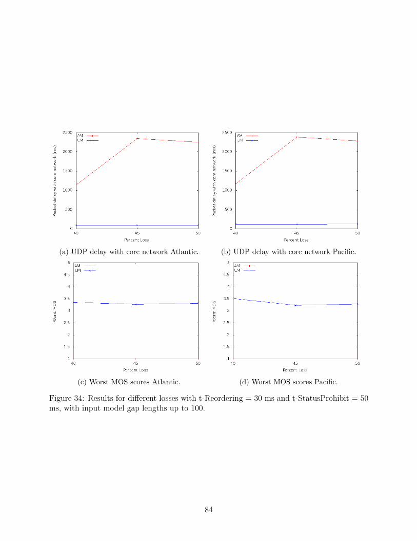
(a) UDP delay with core network Atlantic. (b) UDP delay with core network Pacific.
(c) Worst MOS scores Atlantic. (d) Worst MOS scores Pacific.
Figure 34: Results for different losses with t-Reordering = 30 ms and t-StatusProhibit = 50ms, with input model gap lengths up to 100.
84
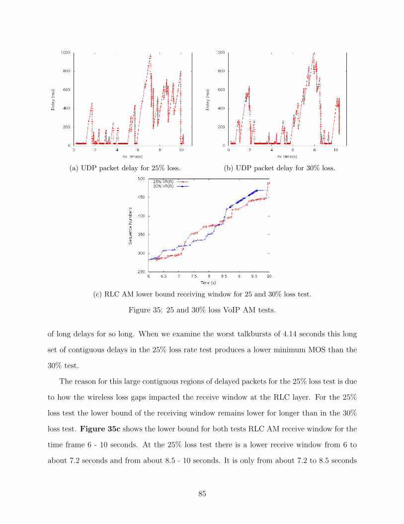
(a) UDP packet delay for 25% loss. (b) UDP packet delay for 30% loss.
(c) RLC AM lower bound receiving window for 25 and 30% loss test.
Figure 35: 25 and 30% loss VoIP AM tests.
of long delays for so long. When we examine the worst talkbursts of 4.14 seconds this long
set of contiguous delays in the 25% loss rate test produces a lower minimum MOS than the
30% test.
The reason for this large contiguous regions of delayed packets for the 25% loss test is due
to how the wireless loss gaps impacted the receive window at the RLC layer. For the 25%
loss test the lower bound of the receiving window remains lower for longer than in the 30%
loss test. Figure 35c shows the lower bound for both tests RLC AM receive window for the
time frame 6 - 10 seconds. At the 25% loss test there is a lower receive window from 6 to
about 7.2 seconds and from about 8.5 - 10 seconds. It is only from about 7.2 to 8.5 seconds
85
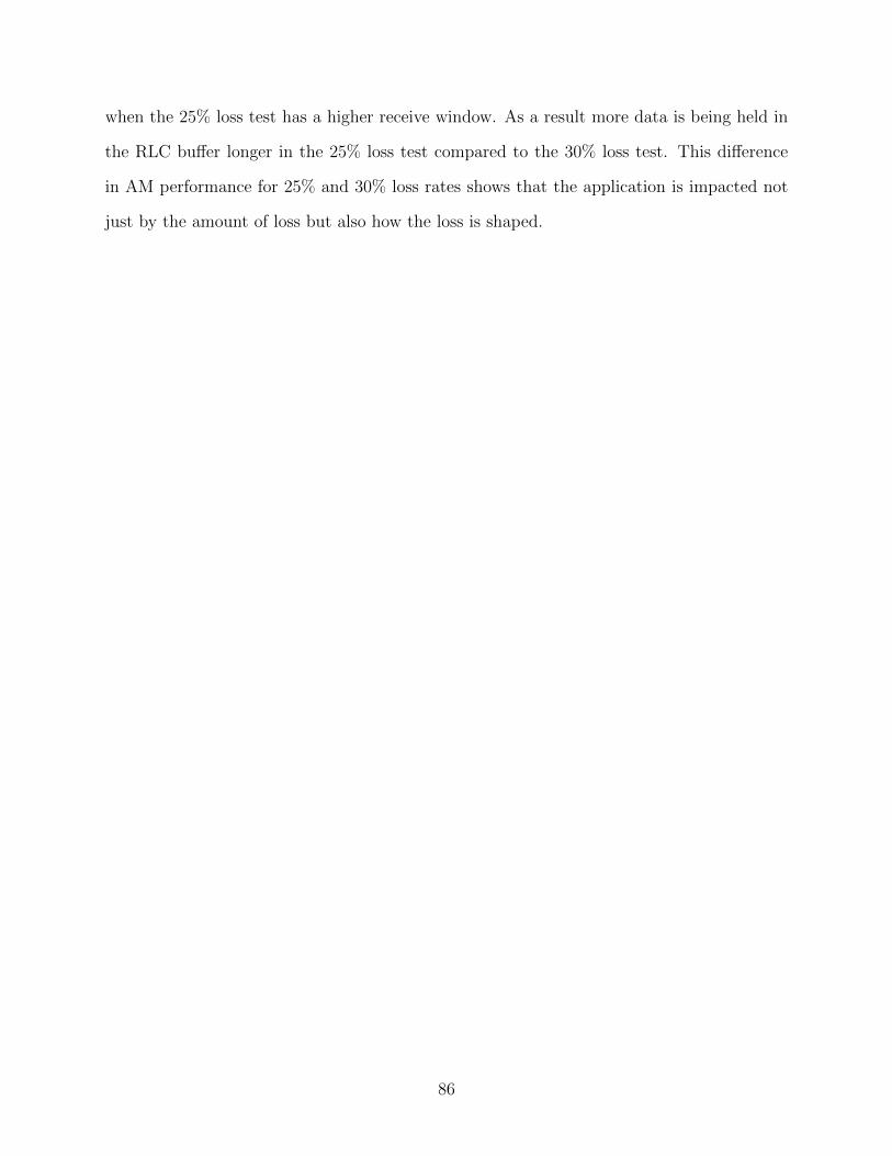
when the 25% loss test has a higher receive window. As a result more data is being held in
the RLC buffer longer in the 25% loss test compared to the 30% loss test. This difference
in AM performance for 25% and 30% loss rates shows that the application is impacted not
just by the amount of loss but also how the loss is shaped.
86
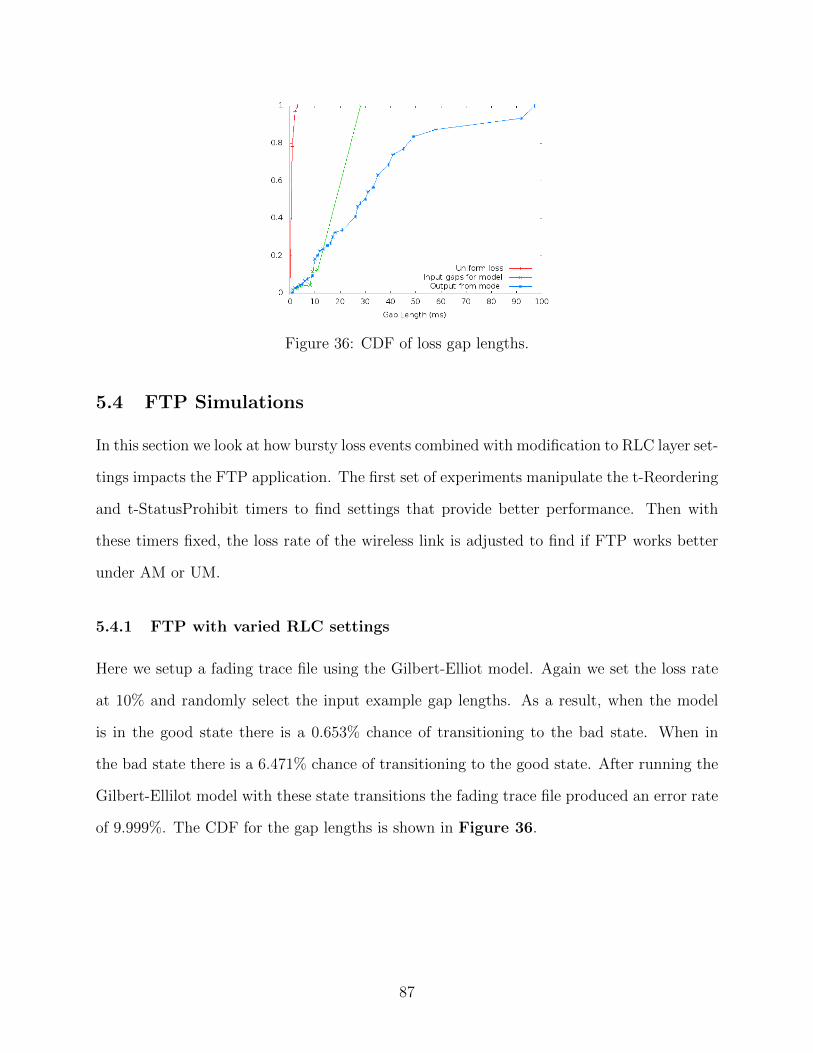
Figure 36: CDF of loss gap lengths.
5.4 FTP Simulations
In this section we look at how bursty loss events combined with modification to RLC layer set-
tings impacts the FTP application. The first set of experiments manipulate the t-Reordering
and t-StatusProhibit timers to find settings that provide better performance. Then with
these timers fixed, the loss rate of the wireless link is adjusted to find if FTP works better
under AM or UM.
5.4.1 FTP with varied RLC settings
Here we setup a fading trace file using the Gilbert-Elliot model. Again we set the loss rate
at 10% and randomly select the input example gap lengths. As a result, when the model
is in the good state there is a 0.653% chance of transitioning to the bad state. When in
the bad state there is a 6.471% chance of transitioning to the good state. After running the
Gilbert-Ellilot model with these state transitions the fading trace file produced an error rate
of 9.999%. The CDF for the gap lengths is shown in Figure 36.
87

Table 7: FTP results AM t-Reordering
t-Reordering Average Mb/s Standard Dev Mb/s0 5.2 2.25 4.0 1.910 4.6 2.215 5.1 2.520 4.4 1.925 2.3 1.330 2.3 1.335 2.3 1.340 2.5 1.350 4.7 1.960 4.4 2.070 5.2 1.980 5.3 2.390 5.0 2.1100 3.4 2.0110 4.4 2.2120 3.9 2.2130 4.3 2.0140 3.7 2.1150 3.4 1.5160 3.6 1.7170 3.6 1.7180 3.6 1.7190 4.0 1.6200 3.6 1.7
5.4.1.1 t-Reordering
The results of adjusting the timer t-Reordering for AM and UM are shown in Tables 7 and
8 respectively. These tables list the average and standard deviation of the TCP throughput
seen at the receiver. The standard deviations range from 0.2 - 2.5 Mb/s. The reason for
the large standard deviation comes from TCP RTOs. When the TCP data or TCP ACKs
are lost the sending server can see long delays from arriving ACKs. If this delay is too long
TCP experiences RTOs and lowers cwnd to 1 segment size. TCP returns to slow start. The
results for t-Reordering are also shown in Figure 37.
The throughput In Figure 37 generally gets worse as the setting of t-Reordering in-
88
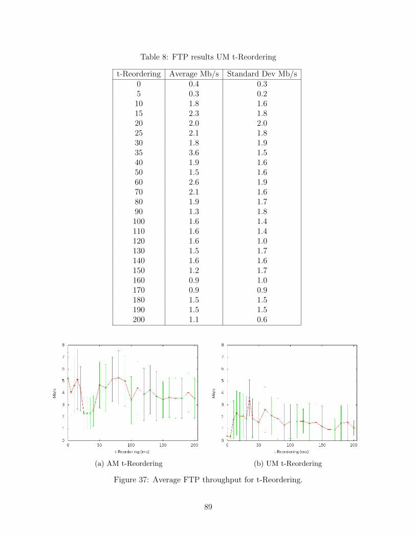
Table 8: FTP results UM t-Reordering
t-Reordering Average Mb/s Standard Dev Mb/s0 0.4 0.35 0.3 0.210 1.8 1.615 2.3 1.820 2.0 2.025 2.1 1.830 1.8 1.935 3.6 1.540 1.9 1.650 1.5 1.660 2.6 1.970 2.1 1.680 1.9 1.790 1.3 1.8100 1.6 1.4110 1.6 1.4120 1.6 1.0130 1.5 1.7140 1.6 1.6150 1.2 1.7160 0.9 1.0170 0.9 0.9180 1.5 1.5190 1.5 1.5200 1.1 0.6
(a) AM t-Reordering (b) UM t-Reordering
Figure 37: Average FTP throughput for t-Reordering.
89
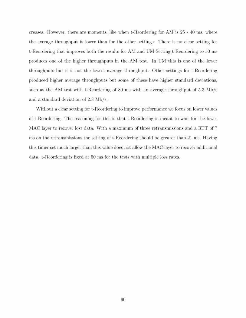
creases. However, there are moments, like when t-Reordering for AM is 25 - 40 ms, where
the average throughput is lower than for the other settings. There is no clear setting for
t-Reordering that improves both the results for AM and UM Setting t-Reordering to 50 ms
produces one of the higher throughputs in the AM test. In UM this is one of the lower
throughputs but it is not the lowest average throughput. Other settings for t-Reordering
produced higher average throughputs but some of these have higher standard deviations,
such as the AM test with t-Reordering of 80 ms with an average throughput of 5.3 Mb/s
and a standard deviation of 2.3 Mb/s.
Without a clear setting for t-Reordering to improve performance we focus on lower values
of t-Reordering. The reasoning for this is that t-Reordering is meant to wait for the lower
MAC layer to recover lost data. With a maximum of three retransmissions and a RTT of 7
ms on the retransmissions the setting of t-Reordering should be greater than 21 ms. Having
this timer set much larger than this value does not allow the MAC layer to recover additional
data. t-Reordering is fixed at 50 ms for the tests with multiple loss rates.
90

Table 9: FTP results AM t-StatusProhibit
t-StatusProhibit Average Mb/s Standard Dev Mb/s0 2.9 1.55 4.4 3.210 3.9 2.115 4.2 1.820 2.5 1.325 3.7 2.550 4.9 2.375 5.5 2.1100 4.7 2.1125 3.8 1.8150 4.7 1.9175 3.1 2.0200 3.5 1.6225 2.7 1.6250 2.5 1.9300 2.9 1.3350 2.3 2.1400 3.7 2.1450 3.7 2.1500 1.6 1.1
5.4.1.2 t-StatusProhibit
The result of adjusting t-StatusProhibit also has a high standard deviation as seen in Table
9. Here delaying STATUS messages that could recover lost data or increasing the rate of
STATUS messages, removing opportunities to transmit data, negatively impact the average
throughput and the standard deviation seen. The results of both the t-StatusProhibit are
also shown in Figure 38.
In Figure 38, as the setting on t-StatusProhibit increases the average throughput tends
to decrease. Like with the setting of t-Reordering this is not always true as some higher
settings of t-StatusProhibit produces higher throughputs. Unlike the tests with t-Reordering
there is one setting that produces a noticeable improvement in throughput. In the following
tests with varied loss rates the timer t-StatusPrhobit is set to 75 ms.
91

Figure 38: AM t-StatusProhibit
Figure 39: Average FTP throughput for t-StatusProhibit.
92
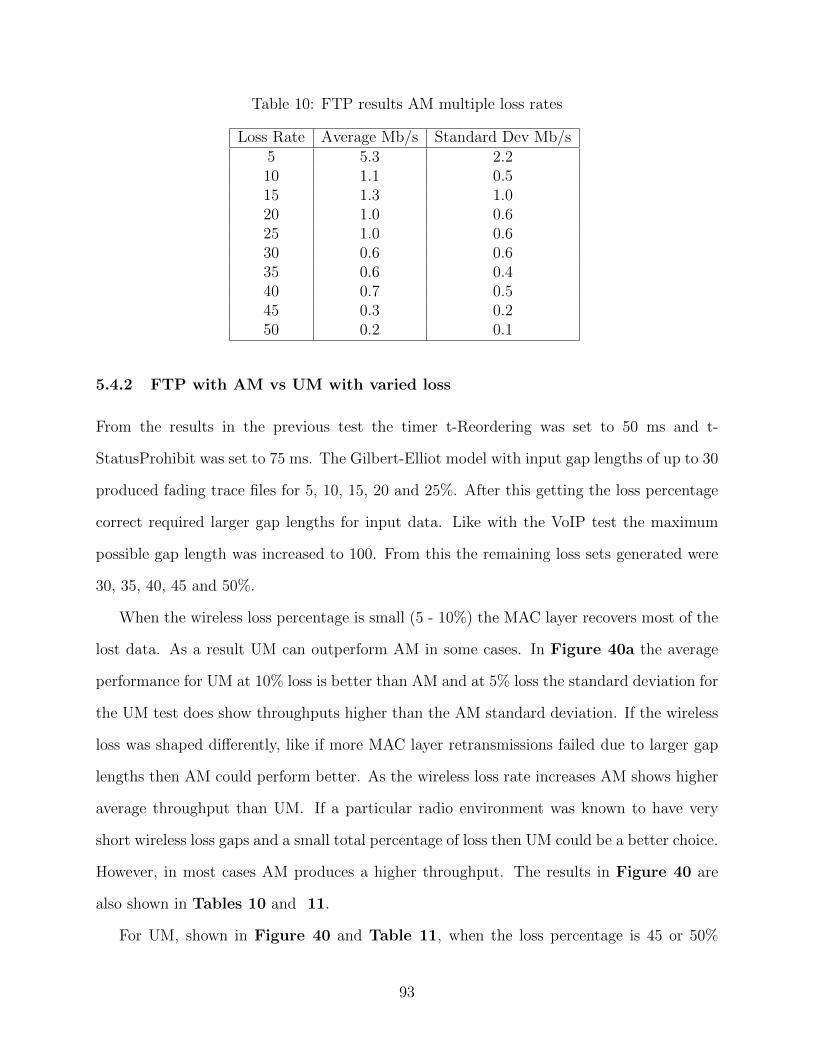
Table 10: FTP results AM multiple loss rates
Loss Rate Average Mb/s Standard Dev Mb/s5 5.3 2.210 1.1 0.515 1.3 1.020 1.0 0.625 1.0 0.630 0.6 0.635 0.6 0.440 0.7 0.545 0.3 0.250 0.2 0.1
5.4.2 FTP with AM vs UM with varied loss
From the results in the previous test the timer t-Reordering was set to 50 ms and t-
StatusProhibit was set to 75 ms. The Gilbert-Elliot model with input gap lengths of up to 30
produced fading trace files for 5, 10, 15, 20 and 25%. After this getting the loss percentage
correct required larger gap lengths for input data. Like with the VoIP test the maximum
possible gap length was increased to 100. From this the remaining loss sets generated were
30, 35, 40, 45 and 50%.
When the wireless loss percentage is small (5 - 10%) the MAC layer recovers most of the
lost data. As a result UM can outperform AM in some cases. In Figure 40a the average
performance for UM at 10% loss is better than AM and at 5% loss the standard deviation for
the UM test does show throughputs higher than the AM standard deviation. If the wireless
loss was shaped differently, like if more MAC layer retransmissions failed due to larger gap
lengths then AM could perform better. As the wireless loss rate increases AM shows higher
average throughput than UM. If a particular radio environment was known to have very
short wireless loss gaps and a small total percentage of loss then UM could be a better choice.
However, in most cases AM produces a higher throughput. The results in Figure 40 are
also shown in Tables 10 and 11.
For UM, shown in Figure 40 and Table 11, when the loss percentage is 45 or 50%
93
(a) Input gap lengths maximum of 30. (b) Input gap lengths maximum of 100.
Figure 40: Average FTP throughput for t-Reordering = 50 ms and t-StatusProhibit = 75ms
Table 11: FTP results UM multiple loss rates
Loss Rate Average Mb/s Standard Dev Mb/s5 4.8 3.110 1.6 0.915 0.8 0.620 0.2 0.125 0.2 0.230 0.2 0.335 0.2 0.240 0.1 0.145 0.1 0.050 0.1 0.1
94
very little data is received. For example, when the loss rate is 45% the data is only received
for about 2 seconds out of the 10 seconds that sender was transmitting TCP data. The
other data sent was lost before the congestion window had a chance to leave TCP slow start.
This is why the standard deviation for UM at 45% loss is 0, there was just not enough data
received to see variation.
The UE running AM at 45% loss on the other hand receives data for every second of
the simulation thanks to the RLC layer retransmissions. The overall TCP throughput is low
with an average of 0.3 Mb/s due to all the losses but it does receive more data than UM.
Other than the average throughput being lower the fact that UM can go for seconds without
receiving any data suggests that application layer connections could experience socket and
connection timeouts. AM on the other hand manages to keep at least some data arriving to
keep connection and socket timeouts from occurring.
95
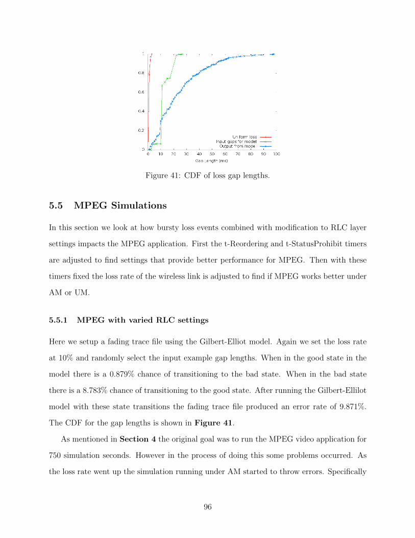
Figure 41: CDF of loss gap lengths.
5.5 MPEG Simulations
In this section we look at how bursty loss events combined with modification to RLC layer
settings impacts the MPEG application. First the t-Reordering and t-StatusProhibit timers
are adjusted to find settings that provide better performance for MPEG. Then with these
timers fixed the loss rate of the wireless link is adjusted to find if MPEG works better under
AM or UM.
5.5.1 MPEG with varied RLC settings
Here we setup a fading trace file using the Gilbert-Elliot model. Again we set the loss rate
at 10% and randomly select the input example gap lengths. When in the good state in the
model there is a 0.879% chance of transitioning to the bad state. When in the bad state
there is a 8.783% chance of transitioning to the good state. After running the Gilbert-Ellilot
model with these state transitions the fading trace file produced an error rate of 9.871%.
The CDF for the gap lengths is shown in Figure 41.
As mentioned in Section 4 the original goal was to run the MPEG video application for
750 simulation seconds. However in the process of doing this some problems occurred. As
the loss rate went up the simulation running under AM started to throw errors. Specifically
96
a test in the LTE simulation module stopped the simulation because a set piece of data
in some of the packet headers was not valid. This indicated to the simulator that some
error occurred while writing, reading or transporting data. After examining the code it
appears that a high load on AM from sending large amounts of data (the video) compared
to the amount of available bandwidth (transport block size) along with the need for many
retransmissions exposed this problem. Unfortunately, there was not enough time to fully
debug and fix this issue. This bug did not impact the other simulations run as the test in
the simulator code catches and ends any simulation that experiences the error. This error
only occurred after about 450 seconds of simulation time. To avoid this error the amount of
time to run the MPEG video simulation was set to 300 seconds.
The following tests show the average delay of receiving the MPEG frames. For UM we
also report the percent of frames lost. A frame loss is defined as a frame having any of its
UDP packets lost or any frame whose dependent frame is lost. As mentioned earlier MPEG
has I, P and B frames where P frames are dependent on the previous I or P frame and B
frames are dependent on the past or previous I or P frame. The sample trace file for the
video sends frames in the order I, P, B, B, P, B, B, P, B, B and then repeats. Any B frame
loss is just that frame. Any I or P frame loss causes losses for all following frames up to the
next I or B frame preceding an arrived I frame.
97
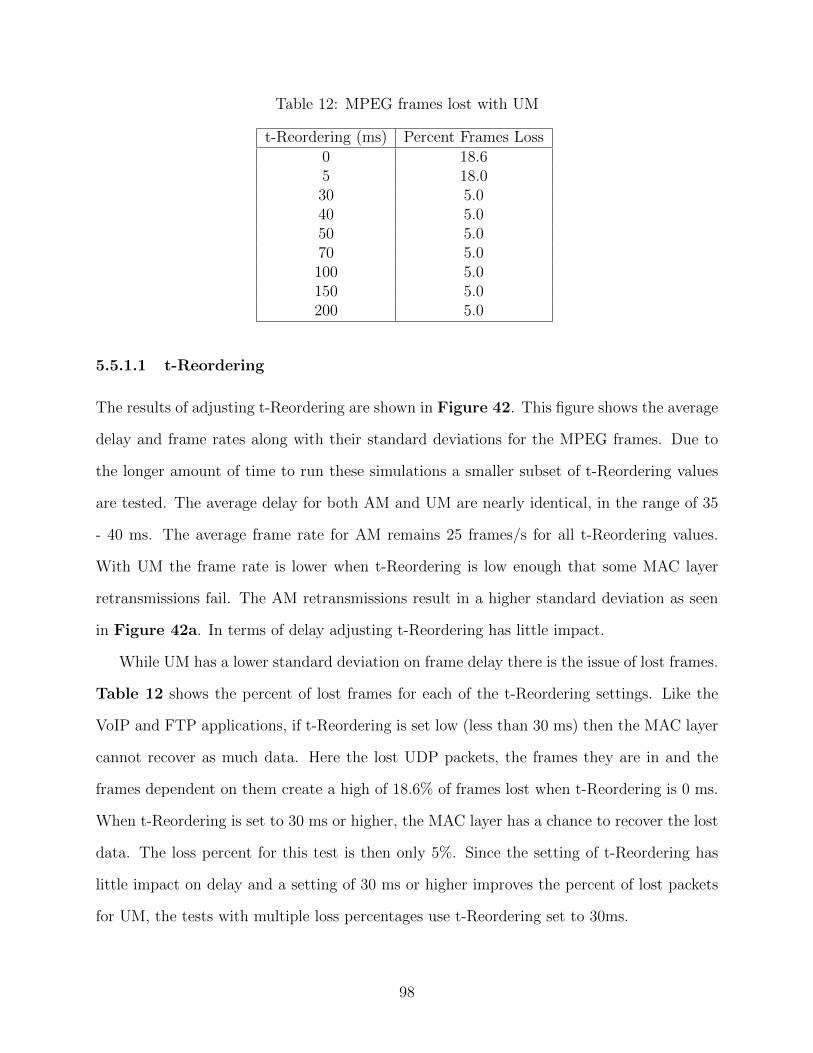
Table 12: MPEG frames lost with UM
t-Reordering (ms) Percent Frames Loss0 18.65 18.030 5.040 5.050 5.070 5.0100 5.0150 5.0200 5.0
5.5.1.1 t-Reordering
The results of adjusting t-Reordering are shown in Figure 42. This figure shows the average
delay and frame rates along with their standard deviations for the MPEG frames. Due to
the longer amount of time to run these simulations a smaller subset of t-Reordering values
are tested. The average delay for both AM and UM are nearly identical, in the range of 35
- 40 ms. The average frame rate for AM remains 25 frames/s for all t-Reordering values.
With UM the frame rate is lower when t-Reordering is low enough that some MAC layer
retransmissions fail. The AM retransmissions result in a higher standard deviation as seen
in Figure 42a. In terms of delay adjusting t-Reordering has little impact.
While UM has a lower standard deviation on frame delay there is the issue of lost frames.
Table 12 shows the percent of lost frames for each of the t-Reordering settings. Like the
VoIP and FTP applications, if t-Reordering is set low (less than 30 ms) then the MAC layer
cannot recover as much data. Here the lost UDP packets, the frames they are in and the
frames dependent on them create a high of 18.6% of frames lost when t-Reordering is 0 ms.
When t-Reordering is set to 30 ms or higher, the MAC layer has a chance to recover the lost
data. The loss percent for this test is then only 5%. Since the setting of t-Reordering has
little impact on delay and a setting of 30 ms or higher improves the percent of lost packets
for UM, the tests with multiple loss percentages use t-Reordering set to 30ms.
98
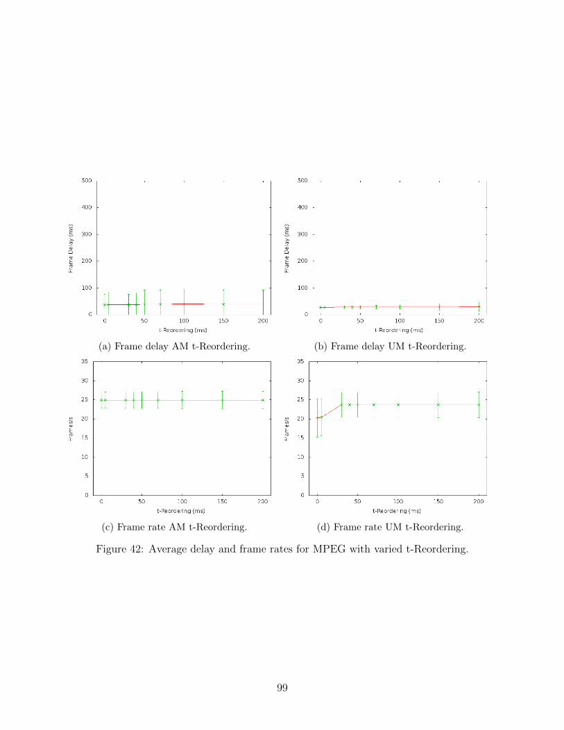
(a) Frame delay AM t-Reordering. (b) Frame delay UM t-Reordering.
(c) Frame rate AM t-Reordering. (d) Frame rate UM t-Reordering.
Figure 42: Average delay and frame rates for MPEG with varied t-Reordering.
99
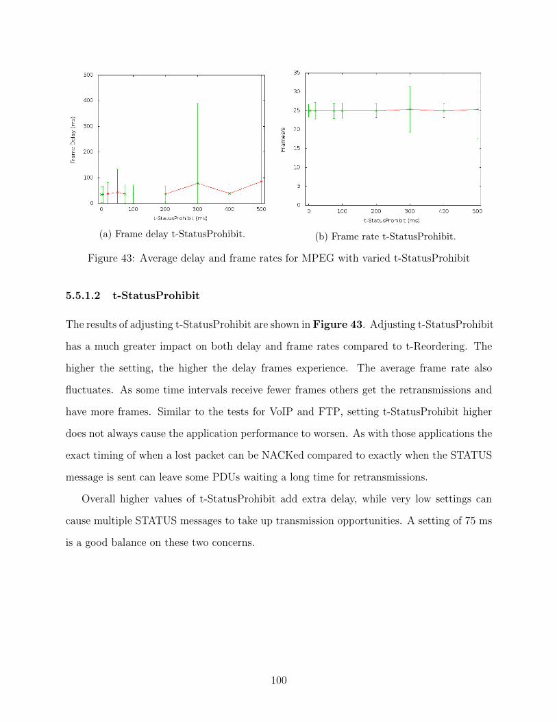
(a) Frame delay t-StatusProhibit. (b) Frame rate t-StatusProhibit.
Figure 43: Average delay and frame rates for MPEG with varied t-StatusProhibit
5.5.1.2 t-StatusProhibit
The results of adjusting t-StatusProhibit are shown in Figure 43. Adjusting t-StatusProhibit
has a much greater impact on both delay and frame rates compared to t-Reordering. The
higher the setting, the higher the delay frames experience. The average frame rate also
fluctuates. As some time intervals receive fewer frames others get the retransmissions and
have more frames. Similar to the tests for VoIP and FTP, setting t-StatusProhibit higher
does not always cause the application performance to worsen. As with those applications the
exact timing of when a lost packet can be NACKed compared to exactly when the STATUS
message is sent can leave some PDUs waiting a long time for retransmissions.
Overall higher values of t-StatusProhibit add extra delay, while very low settings can
cause multiple STATUS messages to take up transmission opportunities. A setting of 75 ms
is a good balance on these two concerns.
100
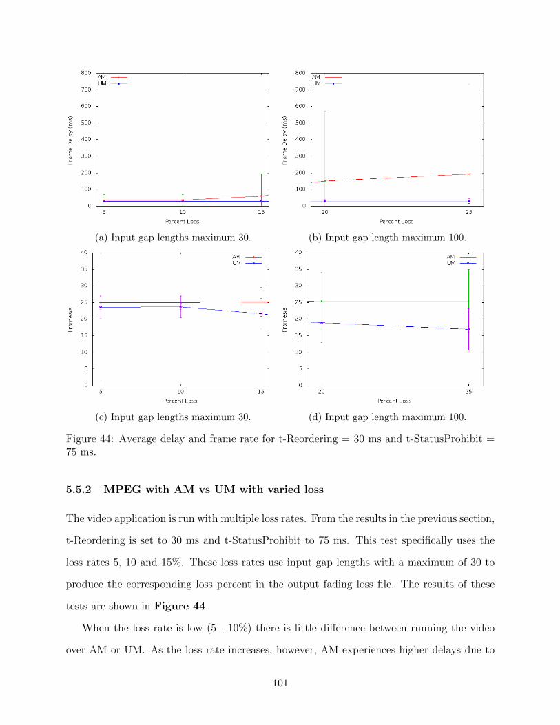
(a) Input gap lengths maximum 30. (b) Input gap length maximum 100.
(c) Input gap lengths maximum 30. (d) Input gap length maximum 100.
Figure 44: Average delay and frame rate for t-Reordering = 30 ms and t-StatusProhibit =75 ms.
5.5.2 MPEG with AM vs UM with varied loss
The video application is run with multiple loss rates. From the results in the previous section,
t-Reordering is set to 30 ms and t-StatusProhibit to 75 ms. This test specifically uses the
loss rates 5, 10 and 15%. These loss rates use input gap lengths with a maximum of 30 to
produce the corresponding loss percent in the output fading loss file. The results of these
tests are shown in Figure 44.
When the loss rate is low (5 - 10%) there is little difference between running the video
over AM or UM. As the loss rate increases, however, AM experiences higher delays due to
101
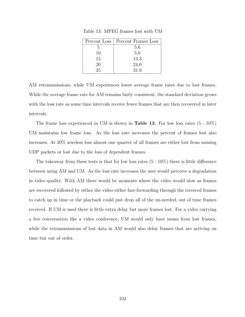
Table 13: MPEG frames lost with UM
Percent Loss Percent Frames Loss5 5.610 5.015 13.320 24.025 31.9
AM retransmissions, while UM experiences lower average frame rates due to lost frames.
While the average frame rate for AM remains fairly consistent, the standard deviation grows
with the loss rate as some time intervals receive fewer frames that are then recovered in later
intervals.
The frame loss experienced in UM is shown in Table 13. For low loss rates (5 - 10%)
UM maintains low frame loss. As the loss rate increases the percent of frames lost also
increases. At 20% wireless loss almost one quarter of all frames are either lost from missing
UDP packets or lost due to the loss of dependent frames.
The takeaway from these tests is that for low loss rates (5 - 10%) there is little difference
between using AM and UM. As the loss rate increases the user would perceive a degradation
in video quality. With AM there would be moments where the video would slow as frames
are recovered followed by either the video either fast-forwarding through the received frames
to catch up in time or the playback could just drop all of the un-needed, out of time frames
received. If UM is used there is little extra delay but more frames lost. For a video carrying
a live conversation like a video conference, UM would only have issues from lost frames,
while the retransmissions of lost data in AM would also delay frames that are arriving on
time but out of order.
102
6 Conclusion
This work examines how retransmissions in 4G LTE impact VoIP, FTP and video appli-
cations. VoIP and video over UDP are sensitive to delay and the amount of data lost in
transit. FTP is sensitive to the throughput of data. In LTE, retransmissions occur between
the eNodeB and UE at both the MAC and RLC layers. In the RLC layer there are choices
for either using retransmissions or not (AM and UM). In addition, the RLC layer has config-
uration parameters to set how long to wait for the MAC layer to recover data (t-Reordering)
and the minimum time to wait in-between sending ACKs and NACKs between the eNodeB
and UE.
To test the impact of 4G LTE retransmissions, we used the open source ns-3 packet
network simulator, which has a LTE module. This module did not support sending NACKs
in RLC AM STATUS messages. We added this capability to the simulator and sent these
changes back to the developers of the module. We ran six experiments with two nodes over
a range of loss and latency conditions.
In the VoIP simulations, the benefit of extra retransmissions in AM improved call quality
up to a 20% loss of data on the wireless link. After this, the added delay of retransmissions
was more detrimental to the total lost packets. The values for timers t-Reordering and t-
StatusProhibit were set to 30 ms and 50 ms respectively. With t-Reordering at 30 ms the
MAC layer has a chance to recover lost data that a lower setting could lose in UM. Higher
settings to t-Reordering can delay retransmissions of lost data in AM, although this impact
was small. For t-StatusProhibit at 75 ms, a STATUS message of ACKs and NACKs can
only be sent at least once every 75 ms. Smaller settings did not improve performance, while
higher settings greatly reduced the call quality.
The FTP simulations maintain a higher TCP throughput when using AM as opposed
to UM. The additional LTE retransmissions reduce the number of TCP retransmissions
required. However, large numbers of TCP RTOs cause great variability in throughputs. This
103
is especially true when using AM since the TCP layer must wait for the LTE retransmissions
without any feedback. The RLC timers t-Reordering and t-StatusProhibit were set to 50
ms and 75 ms respectively. During testing, lower values of t-Reordering produced higher
throughput though some lower settings such as 25 - 40 ms produced a much lower throughput
when using AM. Similarly t-StatusProhibit also produced higher throughputs for lower
settings. However, very low settings of this timer increase the number of STATUS messages,
taking away from application data transmission opportunities.
The MPEG video simulations show that UM maintains a lower average delay between
27 and 30 ms with low frame loss compared to AM, with average delays between 35 and 200
ms. However, while UM maintains a lower average delay the resulting lost frames mean that
UM has a lower average frame rate. When using AM the lost frames are recovered, but the
video experiences a much larger variation in frame rates as losses in one time interval can
lead to more frames arriving (due to retransmissions) in another. While UM experiences
increasing frame loss with an increase in wireless loss, those frames that arrive without error
have little delay while in AM frames that arrive correctly but out of order need to wait for
the AM retransmissions. For the VoIP and FTP applications, the settings of t-Reordering
and t-StatusProhibit produce lower delays for MPEG video when the timers are set within
the range of tens of milliseconds. t-Reordering was set to 30 ms and t-StatusProhibit to 75
ms.
Delay sensitive applications like VoIP and UDP-based video have better performance
when run over RLC UM while throughput sensitive applications like FTP perform better
with the extra retransmissions of AM. Of the RLC settings examined, the timer t-Reordering
is best set at least high enough to allow the MAC layer to recover all the lost data it can.
The timer t-StatusProhibit is best set low enough to not adversely delay ACKs and NACKs
but not so low that the network spends all of its transmission opportunities sending AM
STATUS messages instead of application data. While there are other RLC retransmission
settings and other types of applications, these simulations show some of the features network
104
providers can expect for some of the common applications they carry on their networks.
LTE networks should set the value of the RLC layer timers based on the type of ap-
plication in use. This is partially possible today through the use of QoS classes. Section
2.1.2 notes that there is one RLC entity for each QoS class. Each RLC entity could set the
timers t-Reordering and t-StatusProhibit, along with the choice to use AM or UM, to best
handle the traffic they carry. Today traffic is mapped to these classes using traffic direction
(downlink or uplink), IP address, port number and transport protocol. This granularity is
not sufficient. For instance a VoIP application over UDP and a UDP MPEG video would not
necessarily map to different QoS classes. What is needed in LTE is a method for applications
to indicate to the LTE network layers what settings they require.
105
7 Future Work
Future work would in this area includes expanding on the applications, RLC layer settings
used in testing and adding more features to the LTE simulator used. The video application
tested used UDP packets, making the video like a live conversation setup where delay is
more important that lost data. Other videos like television shows and movies where no
loss is acceptable would use TCP as the underlying protocol. The default TCP congestion
control mechanism used here is New Reno. The ns-3 simulator needs newer methods like
BIC, CUBIC and Compound to provide more realistic simulators of what would happen in
modern networks.
At the RLC layer there are more settings related to retransmissions that need testing.
The timer t-PollRetransmit controls the time the sender waits before re-sending a request
for an AM STATUS message. Linked to this setting are the flags pollPDU and pollByte.
These flags indicate how many PDUs or bytes a node is allowed to send before requesting
the AM STATUS message. These settings impact when AM uses STATUS messages and
therefore impacts when PDUs can be ACKed or NACKed.
The LTE simulator in ns-3 is still under active development and could use more features
that are in LTE. The RLC layer keeps a maximum retransmission count for PDUs when
using AM. Currently the simulator does not use this information. Additions are needed so
that the proper RRC layer control mechanism operate when a PDU is retransmitted more
than the AM maximum. Also while the simulator currently supports packing multiple IP
frames into a single RLC PDU it does not yet support the ability to segment these frames
(encased inside PDCP layer PDUs across multiple RLC layer PDUs). This feature would
reduced empty portions of transport blocks transmitted that could have fit additional data.
106
References
[1] 3GPP. 3rd Genervation Partnership Project; Technical Specification Group Ra-
dio Access Network; Evolved Universal Terrestrial Radio Access (E-UTRA) and
Evoloved Universal Terrestrial Radio Access Network (E-UTRAN); Overall descrip-
tion; stage 2(Release 8). Technical Specification 36.300v8.0.0, 3GPP, march 2007.
http://www.3gpp.org/ftp/Specs/html-info/36300.htm.
[2] 3GPP. 3rd Genervation Partnership Project; Technical Specification Group Radio
Access Network; Evolved Universal Terrestrial Radio Access (E-UTRA); Radio Link
Control (RLC) protocol specification (Release 8). Technical Specification 36.322v8.0.0,
3GPP, December 2007. http://www.3gpp.org/ftp/Specs/html-info/36322.htm.
[3] 3GPP. 3rd Genervation Partnership Project; Technical Specification Group Radio Ac-
cess Network; Evolved Universal Terrestrial Radio Access (E-UTRA) Medium Access
Control (MAC) protocol specification (Release 8). Technical Specification 36.321v8.2.0,
3GPP, May 2008. http://www.3gpp.org/ftp/Specs/html-info/36321.htm.
[4] 3GPP. 3rd Genervation Partnership Project; Technical Specification Group Radio Ac-
cess Network; Evolved Universal Terrestrial Radio Access (E-UTRA); Physical layer
procedures (Release 8). Technical Specification 36.213v8.4.0, 3GPP, September 2008.
http://www.3gpp.org/ftp/Specs/html-info/36213.htm.
[5] 3GPP. 3rd Genervation Partnership Project; Technical Specification Group Radio Ac-
cess Network; Evolved Universal Terrestrial Radio Access (E-UTRA); Radio Resource
Control (RRC) Protocol specification (Release 8). Technical Specification 36.331v8.10.0,
3GPP, march 2008. http://www.3gpp.org/ftp/Specs/html-info/36331.htm.
107
[6] 3GPP. UTRA-UTRAN Long Term Evolution (LTE) and 3GPP Sys-
tem Architecture Evolution (SAE). Technical report, 3GPP, 2008.
ftp://ftp.3gpp.org/Inbox/2008%5Fweb%5Ffiles/LTA%5FPaper.pdf.
[7] 3GPP. Universal Mobile Telecommunications System (UMTS); User
Equipment (UE) conformance specification; Radio transmission and re-
ception (FDD); Part 1: Conformance specification (3GPP TS 34.121-
1 version 8.8.0 Release 8). Technical Specification 34.121-1v8.8.0, 3GPP,
2009. http://www.etsi.org/deliver/etsi ts/134100 134199/13412101/08.08.00 60/
ts 13412101v080800p.pdf.
[8] 3GPP. 3rd Generation Partnership Project; Technical Specification Group Radio Access
Network; Evolved Universal Terrestrial Radio Access (E-UTRA); Base Station (BS)
radio transmission and reception (Release 8). Technical Specification 36.104v8.13.0,
3GPP, 2012. http://www.3gpp.org/DynaReport/36104.htm.
[9] A. Asheralieva, J.Y. Khan, and K. Mahata. Performance analysis of voip services on the
lte network. In Australasian Telecommunication Networks and Applications Conference
(ATNAC), 2011, pages 1–6, Nov 2011.
[10] M. Baldi and Y. Ofek. End-to-end delay analysis of videoconferencing over packet-
switched networks. Networking, IEEE/ACM Transactions on, 8(4):479–492, Aug 2000.
[11] Nicola Baldo, Marco Miozzo, Manuel Requena-Esteso, and Jaume Nin-Guerrero. An
open source product-oriented lte network simulator based on ns-3. In Proceedings of the
14th ACM International Conference on Modeling, Analysis and Simulation of Wireless
and Mobile Systems, MSWiM ’11, pages 293–298, New York, NY, USA, 2011. ACM.
[12] Ricky A Bangun, E Dutkiewicz, and GJ Anido. An analysis of multi-player network
games traffic. In Multimedia Signal Processing, 1999 IEEE 3rd Workshop on, pages
3–8. IEEE, 1999.
108
[13] Matthias Bohmer, Brent Hecht, Johannes Schoning, Antonio Kruger, and Gernot Bauer.
Falling asleep with angry birds, facebook and kindle: a large scale study on mobile appli-
cation usage. In Proceedings of the 13th International Conference on Human Computer
Interaction with Mobile Devices and Services, pages 47–56. ACM, 2011.
[14] Leandro Carvalho, Edjair Mota, Regeane Aguiar, Ana F Lima, Jose Neuman de Souza,
and Anderson Barreto. An E-model implementation for speech quality evaluation in
VoIP systems. In Proceedings of the 10th IEEE Symposium on Computers and Com-
munications, volume 154. IEEE Computer Society, 2005.
[15] Xiuzhong Chen, Chunfeng Wang, Dong Xuan, Zhongcheng Li, Yinghua Min, and Wei
Zhao. Survey on QoS management of VoIP. In Computer Networks and Mobile Comput-
ing, 2003. ICCNMC 2003. 2003 International Conference on, pages 69–77, Oct 2003.
[16] Cisco. Cisco Visual Networking Index: Global Mobile Data Traf-
fic Forecast Update, 2013-2018. Technical report, Cisco, 2014.
http://www.cisco.com/en/US/solutions/collateral/ns341/ns525/ns537/ns705/ns827/
white paper c11-520862.pdf.
[17] Erik Dahlman, Stefan Parkvall, and Johan Skold. 4G LTE/LTE-Advanced for Mobile
Broadband. Academic Press, Oxford, 2011.
[18] DARPA. Transmission Control Protocol. RFC RFC793, DARPA, September 1981.
RFC793.
[19] DARPA. TCP Congestion Control. RFC RF2581, DARPA, April 1999. RFC2581.
[20] H. Ekstrom. QoS Control in the 3GPP Evolved Packet System. Communications
Magazine, IEEE, 47(2):76–83, 2009.
[21] Frederic Firmin. 3GPP The Evolved Packet Core @ONLINE, April 2013.
http://www.3gpp.org/The-Evolved-Packet-Core.
109
[22] Didier Le Gall. Mpeg: A video compression standard for multimedia applications.
Commun. ACM, 34(4):46–58, 1991.
[23] Edgar N Gilbert. Capacity of a burst-noise channel. Bell system technical journal,
39(5):1253–1265, 1960.
[24] N Gordo and A Daniel. Evaluating video quality degradation from data packet losses
in an lte environment. Master’s thesis, Lulea University of Technology, Universitet-
somradet, Porsn, 971 87 Lulea, Sweden, 2009.
[25] Junxian Huang, Feng Qian, Yihua Guo, Yuanyuan Zhou, Qiang Xu, Z. Morley Mao,
Subhabrata Sen, and Oliver Spatscheck. An In-depth Study of LTE: Effect of Network
Protocol and Application Behavior on Performance. In Proceedings of the ACM SIG-
COMM 2013 Conference on SIGCOMM, SIGCOMM ’13, pages 363–374, New York,
NY, USA, 2013. ACM.
[26] Josep Colom Ikuno, Martin Wrulich, and Markus Rupp. Performance and modeling
of lte h-arq. In Proc. International ITG Workshop on Smart Antennas (WSA 2009),
Berlin, Germany, 2009.
[27] Haiqing Jiang, Yaogong Wang, Kyunghan Lee, and Injong Rhee. Tackling bufferbloat in
3g/4g networks. In Proceedings of the 2012 ACM conference on Internet measurement
conference, pages 329–342. ACM, 2012.
[28] Stylianos Karapantazis and Fotini-Niovi Pavlidou. VoIP: A comprehensive survey on a
promising technology. Computer Networks, 53(12):2050–2090, 2009.
[29] T. Mohammad Kawser, Nafix Imtiaz Bin Hamid, Nayeemul Hasan, M. Shah Alam, and
M. Musfiqur Rahman. Limiting HARQ Retransmissions in Downlink for Poor Radio
Link in LTE. International Journal of Information and Electronics Engineering, 2012.
110
[30] Michael Makidis. Implementing and evaluating the RLC/AM protocol of the 3GPP
specification. Master’s thesis, Athens University of Economics and Business, 2007.
[31] Ebna Masum and Jewel Babu. End-to-End Delay Performance Evaluation for VoIP in
the LTE network. Master’s thesis, Blekinge Institue of Technology, 2011.
[32] Christian Mehlfuhrer, Martin Wrulich, J Colom Ikuno, Dagmar Bosanska, and Markus
Rupp. Simulating the long term evolution physical layer. In Proc. of the 17th European
Signal Processing Conference (EUSIPCO 2009), Glasgow, Scotland, volume 27, page
124, 2009.
[33] AC Norwine and OJ Murphy. Characteristic time intervals in telephonic conversation.
Bell System Technical Journal, 17(2):281–291, 1938.
[34] J. Postel. User Datagram Protocol. Technical Report RF768, August 1980. RFC768.
[35] Sanjay Ramroop. A DiffServ model for the NS-3 simulator. Tech-
nical Report 807004374, The University of the West Indies Elec-
trical and Computer Engineering Department, September 2010.
http://www.eng.uwi.tt/depts/elec/staff/rvadams/sramroop/index.htm.
[36] International Telecommunication Union. Pulse Code Movulation (PCM) of
Vlice Frequencies. Technical Specification G.711, ITU-T, November 1988.
https://www.itu.int/rec/dologin pub.asp?lang=e&id=T-REC-G.711-198811-I!!PDF-
E&type=items.
[37] International Telecommunication Union. Methods for subjective determination of trans-
mission quality. Technical Specification P.800, ITU-T, 1996. http://www.itu.int/rec/T-
REC-P.800-199608-I/en.
111
[38] International Telecommunication Union. The E-model, a computational model for
use in transmission planning. Technical Specification G.107, ITU-T, December 1998.
http://www.itu.int/rec/T-REC-G.107-199812-S/en.
[39] International Telecommunication Union. International telephone connections and
circuits - General Recommendations on the transmission quality for an en-
tire international telephone connection. Technical Specification G.114, ITU-T,
May 2003. http://www.itu.int/rec/dologin pub.asp?lang=e&id=T-REC-G.114-200305-
I!!PDF-E&type=items.
[40] Verizon. IP Lagency Sstatistics, April 2014. http://www.verizonenterprise.com/about/
network/latency/.
[41] Qiang Xu, Jeffrey Erman, Alexandre Gerber, Zhuoqing Mao, Jeffrey Pang, and Shobha
Venkataraman. Identifying diverse usage behaviors of smartphone apps. In Proceedings
of the 2011 ACM SIGCOMM conference on Internet measurement conference, pages
329–344. ACM, 2011.
[42] Jim Zyren. Overveiw of the 3GPP Long Trem Evolition Physical Layer. Technical
report, Freescale Semiconductor, 07 2007.
112
A Acronyms
This section lists the acronyms used in this paper.
ACK acknowledgment . . . . . . . . . . . . . . . . . . . . . . . . . . . . . . . . . . . . . . . . . . . . . . . . . . . . . . . . . . . . . . . . . 10
AM acknowledged mode . . . . . . . . . . . . . . . . . . . . . . . . . . . . . . . . . . . . . . . . . . . . . . . . . . . . . . . . . . . . . . . . 2
AMC adaptive modulation and coding . . . . . . . . . . . . . . . . . . . . . . . . . . . . . . . . . . . . . . . . . . . . . . . . 49
API application program interface . . . . . . . . . . . . . . . . . . . . . . . . . . . . . . . . . . . . . . . . . . . . . . . . . . . . 119
BLER block level error rate . . . . . . . . . . . . . . . . . . . . . . . . . . . . . . . . . . . . . . . . . . . . . . . . . . . . . . . . . . . . 5
CBR constant bit rate . . . . . . . . . . . . . . . . . . . . . . . . . . . . . . . . . . . . . . . . . . . . . . . . . . . . . . . . . . . . . . . . .44
CDF cumulative distribution function . . . . . . . . . . . . . . . . . . . . . . . . . . . . . . . . . . . . . . . . . . . . . . . . . 68
cwnd congestion control window. . . . . . . . . . . . . . . . . . . . . . . . . . . . . . . . . . . . . . . . . . . . . . . . . . . . . . . 25
CQI channel quality indicator . . . . . . . . . . . . . . . . . . . . . . . . . . . . . . . . . . . . . . . . . . . . . . . . . . . . . . . . . . vi
DCE direct code execution . . . . . . . . . . . . . . . . . . . . . . . . . . . . . . . . . . . . . . . . . . . . . . . . . . . . . . . . . . . . 44
113
EARFCN E-UTRA absolute radio frequency channel number . . . . . . . . . . . . . . . . . . . . . . . . . 48
eNodeB enhanced node b . . . . . . . . . . . . . . . . . . . . . . . . . . . . . . . . . . . . . . . . . . . . . . . . . . . . . . . . . . . . . . 4
EPC evolved packet core . . . . . . . . . . . . . . . . . . . . . . . . . . . . . . . . . . . . . . . . . . . . . . . . . . . . . . . . . . . . . . . 4
E-UTRA evolved universal mobile telecommunications system terrestrial radio access . . . 4
FDD frequency division duplexing . . . . . . . . . . . . . . . . . . . . . . . . . . . . . . . . . . . . . . . . . . . . . . . . . . . . . 19
FEC forward error correction . . . . . . . . . . . . . . . . . . . . . . . . . . . . . . . . . . . . . . . . . . . . . . . . . . . . . . . . . . 10
FTP file transfer protocol . . . . . . . . . . . . . . . . . . . . . . . . . . . . . . . . . . . . . . . . . . . . . . . . . . . . . . . . . . . . . . iv
GBR guaranteed bit rate . . . . . . . . . . . . . . . . . . . . . . . . . . . . . . . . . . . . . . . . . . . . . . . . . . . . . . . . . . . . . . 18
GPRS general packet radio service . . . . . . . . . . . . . . . . . . . . . . . . . . . . . . . . . . . . . . . . . . . . . . . . . . . . . 4
GSM global system for mobile communications . . . . . . . . . . . . . . . . . . . . . . . . . . . . . . . . . . . . . . . . . 4
HARQ hybrid automatic repeat request . . . . . . . . . . . . . . . . . . . . . . . . . . . . . . . . . . . . . . . . . . . . . . . iv
114
HTTP hypertex transfer protocol . . . . . . . . . . . . . . . . . . . . . . . . . . . . . . . . . . . . . . . . . . . . . . . . . . . . . 34
ICMP Internet control message protocol . . . . . . . . . . . . . . . . . . . . . . . . . . . . . . . . . . . . . . . . . . . . . . .74
IP Internet protocol . . . . . . . . . . . . . . . . . . . . . . . . . . . . . . . . . . . . . . . . . . . . . . . . . . . . . . . . . . . . . . . . . . . . 4
ITU International Telecommunication Union. . . . . . . . . . . . . . . . . . . . . . . . . . . . . . . . . . . . . . . . . . .27
LTE Long Term Evolution . . . . . . . . . . . . . . . . . . . . . . . . . . . . . . . . . . . . . . . . . . . . . . . . . . . . . . . . . . . . . iv
MAC Media Access Control . . . . . . . . . . . . . . . . . . . . . . . . . . . . . . . . . . . . . . . . . . . . . . . . . . . . . . . . . . . . 2
MCS modulation and coding scheme . . . . . . . . . . . . . . . . . . . . . . . . . . . . . . . . . . . . . . . . . . . . . . . . . . . x
MIMO multiple input multiple output . . . . . . . . . . . . . . . . . . . . . . . . . . . . . . . . . . . . . . . . . . . . . . . . . .9
MOS mean opinion score . . . . . . . . . . . . . . . . . . . . . . . . . . . . . . . . . . . . . . . . . . . . . . . . . . . . . . . . . . . . . . 28
MPEG movie picture experts group . . . . . . . . . . . . . . . . . . . . . . . . . . . . . . . . . . . . . . . . . . . . . . . . . . . . v
MTU maximum transmission unit . . . . . . . . . . . . . . . . . . . . . . . . . . . . . . . . . . . . . . . . . . . . . . . . . . . . . 46
115

NACK negative acknowledgment . . . . . . . . . . . . . . . . . . . . . . . . . . . . . . . . . . . . . . . . . . . . . . . . . . . . . . . 2
NAS Non Access Stratum . . . . . . . . . . . . . . . . . . . . . . . . . . . . . . . . . . . . . . . . . . . . . . . . . . . . . . . . . . . . . . 5
NSC network simulation cradle . . . . . . . . . . . . . . . . . . . . . . . . . . . . . . . . . . . . . . . . . . . . . . . . . . . . . . . . 44
OFDM orthogonal frequency-division multiplexing. . . . . . . . . . . . . . . . . . . . . . . . . . . . . . . . . . . . . .6
PDCP Packet Data Convergence Protocol . . . . . . . . . . . . . . . . . . . . . . . . . . . . . . . . . . . . . . . . . . . . . . 5
PDU protocol data unit . . . . . . . . . . . . . . . . . . . . . . . . . . . . . . . . . . . . . . . . . . . . . . . . . . . . . . . . . . . . . . . vii
PGW Packet Delivery Network Gateway . . . . . . . . . . . . . . . . . . . . . . . . . . . . . . . . . . . . . . . . . . . . . . . 4
PRB physical resource block . . . . . . . . . . . . . . . . . . . . . . . . . . . . . . . . . . . . . . . . . . . . . . . . . . . . . . . . . . . . 5
QAM quadrature amplitude modulation . . . . . . . . . . . . . . . . . . . . . . . . . . . . . . . . . . . . . . . . . . . . . . . 34
QoS quality of service . . . . . . . . . . . . . . . . . . . . . . . . . . . . . . . . . . . . . . . . . . . . . . . . . . . . . . . . . . . . . . . . . 16
RLC Radio Link Control . . . . . . . . . . . . . . . . . . . . . . . . . . . . . . . . . . . . . . . . . . . . . . . . . . . . . . . . . . . . . . . iv
116
RRC Radio Resource Control . . . . . . . . . . . . . . . . . . . . . . . . . . . . . . . . . . . . . . . . . . . . . . . . . . . . . . . . . . .5
RTO retransmission time out . . . . . . . . . . . . . . . . . . . . . . . . . . . . . . . . . . . . . . . . . . . . . . . . . . . . . . . . . . 70
RTP real time protocol . . . . . . . . . . . . . . . . . . . . . . . . . . . . . . . . . . . . . . . . . . . . . . . . . . . . . . . . . . . . . . . . 27
RTT round trip time . . . . . . . . . . . . . . . . . . . . . . . . . . . . . . . . . . . . . . . . . . . . . . . . . . . . . . . . . . . . . . . . . . 20
SAE System Architecture Evolution . . . . . . . . . . . . . . . . . . . . . . . . . . . . . . . . . . . . . . . . . . . . . . . . . . . . 4
SDU service data unit . . . . . . . . . . . . . . . . . . . . . . . . . . . . . . . . . . . . . . . . . . . . . . . . . . . . . . . . . . . . . . . . . . 9
SGW Serving Gateway . . . . . . . . . . . . . . . . . . . . . . . . . . . . . . . . . . . . . . . . . . . . . . . . . . . . . . . . . . . . . . . . . 4
ssthresh slow start threshold . . . . . . . . . . . . . . . . . . . . . . . . . . . . . . . . . . . . . . . . . . . . . . . . . . . . . . . . . . 25
SN sequence number. . . . . . . . . . . . . . . . . . . . . . . . . . . . . . . . . . . . . . . . . . . . . . . . . . . . . . . . . . . . . . . . . . .12
SINR signal to noise ratio . . . . . . . . . . . . . . . . . . . . . . . . . . . . . . . . . . . . . . . . . . . . . . . . . . . . . . . . . . . . . . 6
TBS transport block size . . . . . . . . . . . . . . . . . . . . . . . . . . . . . . . . . . . . . . . . . . . . . . . . . . . . . . . . . . . . . . . x
117
TCP transmission control protocol. . . . . . . . . . . . . . . . . . . . . . . . . . . . . . . . . . . . . . . . . . . . . . . . . . . . .25
TDD time division duplexing . . . . . . . . . . . . . . . . . . . . . . . . . . . . . . . . . . . . . . . . . . . . . . . . . . . . . . . . . . 19
TFT traffic flow template . . . . . . . . . . . . . . . . . . . . . . . . . . . . . . . . . . . . . . . . . . . . . . . . . . . . . . . . . . . . . . 17
TM transparent mode . . . . . . . . . . . . . . . . . . . . . . . . . . . . . . . . . . . . . . . . . . . . . . . . . . . . . . . . . . . . . . . . . 10
TTI transmission time interval . . . . . . . . . . . . . . . . . . . . . . . . . . . . . . . . . . . . . . . . . . . . . . . . . . . . . . . . . . 5
UDP user datagram protocol . . . . . . . . . . . . . . . . . . . . . . . . . . . . . . . . . . . . . . . . . . . . . . . . . . . . . . . . . . 26
UE user equipment . . . . . . . . . . . . . . . . . . . . . . . . . . . . . . . . . . . . . . . . . . . . . . . . . . . . . . . . . . . . . . . . . . . . . 4
UM unacknowledged mode . . . . . . . . . . . . . . . . . . . . . . . . . . . . . . . . . . . . . . . . . . . . . . . . . . . . . . . . . . . . 10
UMTS niversal Mobile Telecommunications System . . . . . . . . . . . . . . . . . . . . . . . . . . . . . . . . . . . . 4
VoIP Voice over IP . . . . . . . . . . . . . . . . . . . . . . . . . . . . . . . . . . . . . . . . . . . . . . . . . . . . . . . . . . . . . . . . . . . . iv
118

B CQI
The SINR of the UE has a great impact on the rate at which it can receive data and how
much loss it experiences. While we cannot know what the eNodeB sends to a UE like a
phone without a spectrum analyzer we can know what modulation encoding the phone asks
for. In version 4.2 of the Android application program interface (API) supports getting
information on LTE, including what CQI value the device reports to the tower. To get an
idea of what real life signal quality a user might expect we recorded the CQI reported by
a Samsung Galaxy Nexus smart phone running Android API version 4.2.2. We checked
for this information every 2 minutes but we did not record data when the phone had no
LTE connection. Reasons for missing connections included being connected on a 3G cellular
network or having the device in an area where there was no signal.
We collected this data in Massachusetts. Specifically in the areas of Bristol, Middlesex,
Norfolk, Plymouth and Worcester counties. You can see a subset of the data locations in
Figure 45 where the push-pins show some of the CQI values measured and their approximate
location. During this data collection the phone connected to 81 distinct LTE cells (identified
by cell ID information provided through the Android API).
The phone used to gather this data was carried and used as a normal phone with no
special attention to orientation or placement. The phone was in some cases left on tables,
carried by hand or in pocket. The phone was used as a normal smart phone, which included
making phone calls and applications.
The result of these measurements are shown in Figure 46. Table 1 shows that CQI
values of 1 - 6 indicate QPSK, 7 - 9 is 16QAM and 10 - 15 is 64QAM. Figure 46a shows
CQI measurements categorized by urban and suburban areas, where the phone was mostly
stationary or moving at a walking pace, and traveling roads, where the phone was in a car
traveling at speeds from 40 - 65 miles per hour. In both urban and suburban areas the phone
mostly requested a CQI value of 8. While traveling on roads there was a greater variety of
119
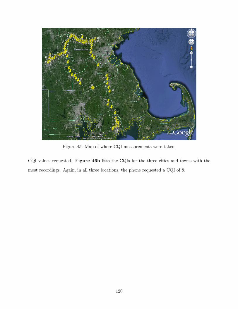
Figure 45: Map of where CQI measurements were taken.
CQI values requested. Figure 46b lists the CQIs for the three cities and towns with the
most recordings. Again, in all three locations, the phone requested a CQI of 8.
120
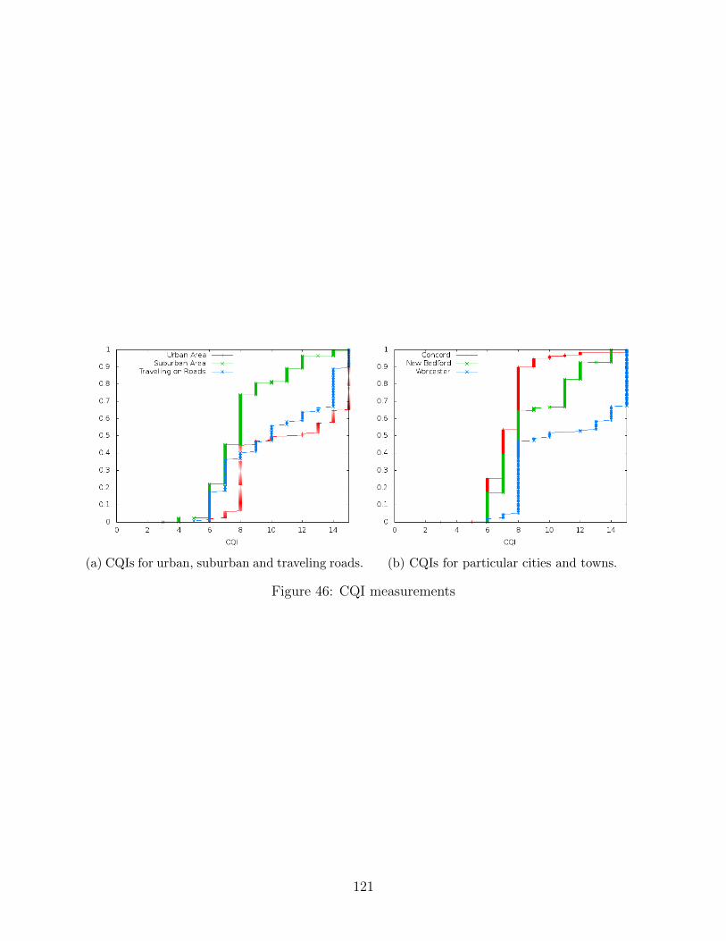
(a) CQIs for urban, suburban and traveling roads. (b) CQIs for particular cities and towns.
Figure 46: CQI measurements
121
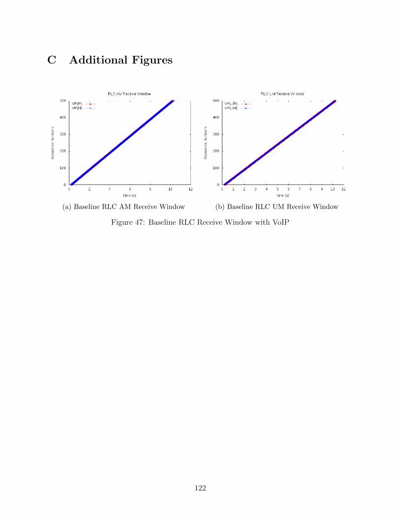
C Additional Figures
(a) Baseline RLC AM Receive Window (b) Baseline RLC UM Receive Window
Figure 47: Baseline RLC Receive Window with VoIP
122

(a) RLC AM Receive Window for UE (b) RLC UM Receive Window for UE.
(c) RLC AM Receive Window for eNodeB. (d) RLC UM Receive Window for eNodeB
Figure 48: Baseline FTP RLC Receive Windows.
Figure 49: Baseline RLC UM receive window for Video.
123
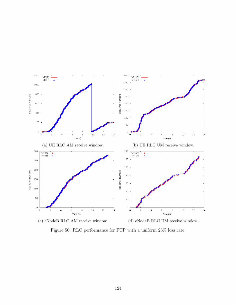
(a) UE RLC AM receive window. (b) UE RLC UM receive window.
(c) eNodeB RLC AM receive window. (d) eNodeB RLC UM receive window.
Figure 50: RLC performance for FTP with a uniform 25% loss rate.
124