IMPACT ASSESSMENT OF FINAL REPORT

I IMPACT ASSESSMENT

I OF REDUCING GASOLINE VOLATILITY

I I

FINAL REPORT

30 NOVEMBER 1983

Prepared for The Research Division

of the Air Resources Board

of the State of California

under Contract No A2-051-32

8(] IJ Bonner ampMoore Management Science I 2727 Allen Parkwaybull Houston Texas 77019 (713) 522-6800 bull TWX 910 881 2542

CAR-8201

The statements and conclusions in this report are

those of the contractor and not necessarily those of

the California Air Resources Board The mention of

commercial products their source or their use in conshy

nection with material reported herein is not to be

construed as either an actual or implied endorsement of

such products

I

ABSTRACT

This report documents a study of the potential impacts on hydrocarbon emissions on vehicle performance and

on refining operations investments and costs of restricting

volatility of gasoline sold in California during the summer

Current volatility limits require a vapor pressure of no

more than 9 psia Assessments of impacts were made for

restrictions of 8 7 and 6 psia fuels in two future situashy

tions based on 1985 and 1990 crude and product forecasts

Results cover emissions effects in terms of vehicular

exhaust and evaporative losses as well as non-vehicular

evaporative losses Vehicle performance effects are defined

in terms of cold start warm-up driveability and safety

considerations Industry-level refining costs are developed

in terms of raw material capital and operating components

Typical refining situations are also examined

Bonner ampMoore Management Bcience

l CAR-8201 i

ACKNOWLEDGMENT

As part of the management of this project ARB

scheduled bi-monthly meetings to review progress and results

Included at these reviews were three representatives from

the refining industry namely Mr HF Bowerman represhy

senting a group of independent refiners Mr W T Danker

representing Chevron USA and Mr T A Wandstrat represhy

senting Shell Oil Company Time spent by these people and

their associates in review of interim results as well as the

study plan and premises provided useful criticism and sugshy

gestions Their efforts as well as those of the various

ARB staff involved with this study are gratefully acknowlshy

edged Particular recognition must be made of the support

provided by Mr Eric Fujita who acted as the technical proshy

ject administrator for ARB

In addition to the various staff within Bonner amp Moore Management Science who assisted in this study the

project team included two subcontractors Mr R W Hurn

of R-H Technical Services Bartlesville Oklahoma who

supplied expertise in the area of vehicle performance Mr

Garrett E Pack of Mittelhauser Corporation El Toro

California conducted the part of this study dealing with

emissions impacts

Bonner ampPMore Managemeft Science CAR-8201 ii

TABLE OF CONTENTS

Paragraph Page

SECTION 1

INTRODUCTION

11 GASOLINE VOLATILITY ITS PURPOSE AND ITS CONTROL------------------------------- 1-2

SECTION 2

SUMMARY OF RESULTS

21 EMISSION IMPACTS SUMMARY------------------ 2-3

22 VEHICLE PERFORMANCE IMPACTS SUMMARY------- 2-7

23 REFINING IMPACTS SUMMARY------------------ 2-8

24 ISSUES NOT COVERED------------------------ 2-15

25 CONCLUSIONS------------------------------- 2-16

26 RECOMMENDATIONS--------------------------- 2-17

SECTION 3

STUDY APPROACH

3 1 EMISSIONS ESTIMATIONS--------------------- 3-1

31 1 Vehicle Classification---------- 3-1

3 1 2 Fuel Factors-------------------- 3-3

3 1 3 Data Base and Calculation Methodology--------------------- 3-5

Bonner ampMoore Managenet 8cience i i iCAR-82O1

TABLE OF CONTENTS (Cont)

Paragraph Page

4322 Gasoline Octane 4-69

4323 Gasoline Sulfur 4-69

433 Refinery Simulator Results------ 4-70

CAR-8201Bomer ampMoore Managemert Science vi

LIST OF APPENDICES

Paragraph Page

APPENDIX A

REFINERY DEMAND FORECASTS A-3

APPENDIX B

CRUDE SUPPLY FORECAST B-3

APPENDIX C

ECONOMIC ASSUMPTIONS C-3

APPENDIX D

SUMMARY OF INTERVIEWS WITH REFINERS---- D-3

APPENDIX E

PRODUCT SPECIFICATIONS---------- E-3

APPENDIX F

MODELING----------------- F-3

APPENDIX G

VEHICLE EMISSIONS PERFORMANCE AND SAFETY--------------------------- G-3

APPENDIX H

VEHICLE EMISSIONS DETAIL--------- H-3

CAR-8201 Bomer ampMoore Management Bcience vii

LIST OF TABLES

Number

2-1 Reactive Organic Emissions Summary From Vehicle and Non-Vehicular Sources---------

2-2 Refining Cost Impacts for Reduced RVP Limits------------------------------------

2-3 Crude Requirements-----------------------shy

2-4 Capital Requirements---------------------shy

2-5 Added Cost - Minimum Action Cases--------shy

4-1 Adjustment of Model-Predicted Distillation Characteristics---------------------------

4-2 Exhaust Emissions Adjustment Factors------

4-3 Estimated California Vehicle Exhaust Emissions---------------------------------

4-4 Evaporative Emissions Adjustment Factors

4-5 Estimated California Vehicle Evaporative Emissions---------------------------------

4-6 Non-Vehicular Emissions-------------------


4-8 Fuel Combustion Emission Factors----------

4-9 Refinery Changes Affecting Process Emissions---------------------------------

4-10 Incremental Refinery Process Emissions (Fuel Oil Displaced by Rejected Hydro-carbons)----------------------------------

4-11 Incremental Refinery Process Emissions (Constant Fuel Oil)-----------------------

4-12 Range of Volatility Characteristics-------

4-13 Changes in Raw Material Cost--------------

4-14 Changes in Raw Material Requirements------

Page

2-6

2-10

2-13

2-13

2-14

4-7

4-10

4-11

4-14

4-17

4-26

4-28

4-33

4-34

4-36

4-37

4-39

4-55

4-56

Bonner ampMoore Management Science CAR-82 0 1 viii

Number

1 l

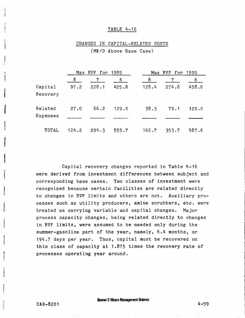
4-15

4-16

4-17

4-18

4-19

4-20

4-21

4-22

4-23

4-24

LIST OF TABLES (Cont)

Increased Energy Requirements------------shy

Changes in Capital-Related Costs---------shy

Changes in Capital Investment------------shy

Changes in Variable Operating Costs------shy

Changes in Total Refining Costs----------shy

Capital Estimates For Rejected Hydrocarbons------------------------------

Sensitivity Analyses Results-------------shy

Added Cost - Minimum Action Cases ($BBL of 9 RVP Production)----------------------

Added Cost - Minimum Action Cases ($BBL of Gasoline at Stated Vapor Pressure)

Gasoline Production - Minimum Action Cases-------------------------------------

Page

4-57

4-59

4-60

4-61

4-62

4-65

4-68

4-75

4-76

4-80

Bonner ampMoore Management 8cienceCAR-8201

I

ix

Figure

2-1

2-2

4-1

4-2

4-3

4-4

4-5

LIST OF ILLUSTRATIONS

Page

RVP Effect on Estimated Emissions 2-5

Refining Cost Impacts for Reduced RVP Limits------------------------------------ 2-9

1980 CRC Intermediate Temperature Program -RVP Effect on Acceleration Stalls-------- 4-44

Flammability of Vapor Over Gasoline------- 4-50

Added Cost $BBL 9 RVP Gasoline (By RVP Within Model Type)---------------- 4-78

Added Costs $BBL 9 RVP Gasoline Produced (By Model Within RVP Class)------ 4-79

Relative Gasoline Production-------------- 4-81

Omner ampMoore Management Science CAR-82 0 1 X

SECTION 1

INTRODUCTION

This report documents a study of impacts resulting from potential restriction of summer gasoline vapor pressure

in the State of California The study was sponsored by the

Research Division of the Air Resources Board (ARB) of the

State of California under contract No A2-051-32 Award of the study contract was made as a consequence of successful

response to a solicitation dated October 27 1981 titled Request for Proposal Entitled Impact of Reducing Gasoline

Volatility in California

The general purpose of this study was to assess the r impacts of lowering the allowable vapor pressure of gasoshy

lines during the summer period Impacts included in these

assessments are effects on hydrocarbon emissions on vehicle

performance on crude requirements on process investments and on refining costs Three more restrictive vapor presshy

sure levels than presently required were studied Impacts

were assessed for two future situations namely projected

environments for 1985 and 1990

Beyond this introductory section this report conshy

tains three other sections and eight appendices Section 2

presents a summary of results Section 3 describes the main elements of the study approach as a framework for the

readers uses of the study results Section 4 presents

detailed results and methodologies Appendix material conshy

tains supporting information

Bonner ampMoore Management Bclence CAR-8201 1-1

The language and contents of this report assume

that readers are familiar with the overall operations of

refining crude oil and the problems of controlling air

quality The report therefore makes use of terms and

references to processes used in petroleum refining and

emissions control without definition On the other hand

the summary of results presented in Section 2 does not

require intimate knowledge of the technologies of refining

or emissions control A brief discussion of the importance

and control of gasoline volatility is present here for those

readers who are not familiar with the subject

11 GASOLINE VOLATILITY ITS PURPOSE AND ITS CONTROL

To function properly as a fuel for spark-ignited

internal-combustion engines gasolines must have certain

volatility characteristics To permit easy starting of a

cold engine the fuel must contain enough low-boiling hydroshy

carbons to provide at ambient temperature an air-fuel-vapor

mixture that is rich enough to be ignited Performance

after starting and during engine warm-up is also influenced

by the concentrations of low-boiling constituents If

however the concentration of low-boiling hydrocarbons is

not restricted the fuel pump (after warm-up) may become

vapor locked and fail to supply enough fuel to support comshy

bustion causing the engine to stall

With the recognition that hydrocarbon emissions

adversely affect air quality evaporative loss of lowshy

boiling hydrocarbons from vehicle fuel systems has become

another reason for concern about gasoline volatility Two

methods have been implemented to reduce fuel system losses

Donner ampMoore Management Science 1-2 CAR-820middot1

One is the use of on-board vapor-collection devices The

other is the reduction of gasoline volatility below the

level required to protect against fuel system vapor-lock

This latter method has been applied only in the State of

California and only to gasoline used during the summer

season On-board vapor-collection devices have the theoreshy

tical potential of restricting evaporative losses regardless

of fuel volatility characteristics and at all ambient conshy

ditions These devices are in general use today being

essentially passive they require little maintenance and are

relatively durable Disadvantages include higher initial

cost potentially inadequate design capacity and potential

for system deterioration and subsequent malfunction

Restricting gasoline volatility has the advantage of reducshy

ing losses throughout distribution and dispensing systems as

well as from the vehicle fuel system Disadvantages include

higher fuel-manufacturing costs and poor vehicle performance

To understand the reasons for the increased cost of lowshy

volatility gasoline it is helpful to review the manner by

which gasoline volatility is controlled during its manufacshy

ture and certain relevant economic factors

As formulated gasoline contains hydrocarbons whose

boiling points range from 58middotF to approximately 400middotF1 The

concentrations of the hydrocarbons in this range are conshy

trolled to satisfy a variety of quality characteristics

including volatility This control is accomplished by the

control of the refining processes which produce gasoline

constituent stocks and by the careful blending of these

1small amounts of hydrocarbons boiling outside this range are usually present because physical separation processes are imperfect

Bomer ampMoore Management 8cience CAR-8201 1-3

intermediate stocks to produce finished gasolines Propershy

ties of blend stocks are determined largely by the nature of

the processes involved but can be varied somewhat by adjustshy

ing operating conditions of those processes Satisfying

quality requirements of finished gasolines is achieved by

controlled blending of available blend stocks

Two measures of volatility are used to obtain

desired cold-start and warm-up characteristics These

measures are Reid Vapor PressureC1) and the volume-percent

boiling below approximately 160middotF(2) These same propershy

ties have been shown to relate to evaporative lossesC3)

They are closely related to the concentration of C4 and C5

hydrocarbons in gasoline and to somewhat lesser extent to

the concentration of C6s Thus control of gasoline volashy

tility is related to the inclusion of these hydrocarbons in

gasoline blend stocks

In particular most refiners have access to normal

butane both as a purchased raw material and as a refinery

stream Historically normal butane has been available as a

by-product from natural gas processing and has been priced

well below that of gasoline Thus the refiner has an

incentive to blend the maximum amount of butane into his

gasoline as limited by vapor-lock considerations A further

incentive is the fact that normal butane has a high octane

rating and thus reduces the cost of meeting octane requireshy

ments of finished gasolines

Summer gasoline in California presently cannot

exceed a Reid Vapor Pressure (RVP) of 90 psi If gasoline

volatility is restricted below present levels refiners must

further restrict the amount of low-boiling hydrocarbons in

their blends This will prevent their using a relatively

inexpensive component as well as require compensating for

Bomer ampMoore Managemert Bclence 1-4 CAR-8201

the octane quality it would provide The first step toward

meeting more restrictive RVP limits would be to restrict (or discontinue) blending butane as such The second step would

be to change processing to exclude butane presently contained

in other blend stocks This could require modification of

existing separation facilities andor the installation of

new facilities to remove contained butanes As a furtherI step extreme RVP limits could require removal of some C5

hydrocarbons which in most cases would require new separashy

tion facilities Not only would the refiner incur additional

costs for removal of these hydrocarbons from gasoline there

l ij

would be a loss in revenue since the rejected materials

would be less valuable in their alternative dispositions

Achieving these alternate dispositions would require capital

expenditures for new facilities such as storage tanks

loading racks lines and pumps Finally additional crudeI and adjusted processing conditions would be required to make

up for the gasoline volume lost by rejecting light hydrocarshy

bons to other dispositions

Honner ampMoore Managemet Bclence CAR-8201 1-5

REFERENCES

(1)ASTM - D-323

( 2 )ASTM - D-86

(3)The Feasibility and Impact of Reducing Hydrocarbon

Emissions by Reducing Gasoline Volatility December 9 1975 State of Californa Air Resources Board

Donner ampMoore Managemeft Bcience 1-6 CAR-8201

SECTION 2

SUMMARY OF RESULTS

I

Impacts assessed in this study and summarized in

this section are limited to those addressed in the work

statement of the original solicitation from ARB They

include impacts on hydrocarbon emissions vehicle performshy

ance refining operations and costs Gasoline volatility

restrictions were defined for this study in terms of vapor

pressure limits Three more restrictive levels than preshy

sently required for summer gasoline have been studied

These are limits of 8 psi 7 psi and 6 psi Two future

situations were examined namely projected environments for

1985 and 1990

Emissions impacts were in part determined from

estimates of changes in vehicle systems behavior These

estimates were made using relationships that have been

developed from results of studies designed to associate

vehicle emissions with fuel volatility characteristics The

volatility characteristics assumed for this study were those

of the gasoline blends derived from projections of future

refinery operations under the various vapor pressure levels

mentioned above Future refining operations were determined

by analyses of the behavior of mathematical models of Calishy

fornias refining facilities

I I

Bonner ampMoore Management Science CAR-8201 2-1

Quantifying impacts of restricting summer gasoline

volatility was the purpose of this study Certain qualitashy

tive results are apparent from making these assessments

namely

1) Limiting vapor pressure to the extreme of 6 RVP would be counter-effective in reducing

hydrocarbon emissions Limiting vapor presshy

sure to 7 RVP may also be counter-effective

2) Exhaust emissions from vehicles would increase

if vapor pressure were restricted to 7 RVP or

less

3) Evaporative emissions from vehicles pre-dating

late 1970 models would improve with reduced

vapor pressure Later model-year vehicles

would probably show little effect

4) Available data on vehicle performance and

emissions is lacking for fuels with low vapor

pressures No data are available for future

vehicle designs

5) Data for existing models indicates that vehishy

cle performance will suffer if vapor pressure

is restricted further than allowed by present

regulations

Dooner ampMoore Management Bcience CAR-8201 2-2

6) At lower limits of vapor pressure decreased driveability and potential for greater exploshysion hazard of fuel tank vapor impact safety considerations

7) Manufacturing costs of gasoline will increase

significantly if vapor pressure is restricted further than allowed by present regulations

Summaries of results from assessment of the various impacts are presented in following subsections This secshy

tion includes a summary of issues not covered as well asr some that were suggested by the study itself Finally

there are subsections presenting conclusions and recommendshy

ations

It should be emphasized that costs identified in

this study pertain to refining impacts Costs related to

automotive design and production and socioeconomic benefits

relating to changes in air quality are not addressed

2 1 EMISSION IMPACTS SUMMARY r A negligible reduction or even an increase in vehishyI cle exhaust emissions is indicated for vapor pressure limits

down to 8 RVP With further reduction in the 7 to 6 RVP

range exhaust emissions are shown to increase by as much as

25 percent For vehicles pre-dating the late 1970s evaposhy

rative emissions would be progressively reduced by as much

as 50 percent Evaporative emissions from late 1970 models

and newer vehicles probably would be negligible This is

because vehicles equipped with current evaporative control technology show little reaction to fuel volatility changes

Bonner amphe~ Hclence CAR-8201 2-3

Emissions from non-vehicular sources would be

reduced if gasoline vapor pressure were further restricted

These sources include refining blending and storage tanks

terminal and transportation facilities and dispensing

operations

Estimated emissions from all sources are summarized

in Table 2-1 Also shown is the net change in estimated

emissions at limits of 8 7 and 6 RVP

The overriding effect of increased exhaust emission

estimates at lower RVP limits is illustrated graphically in

Figure 2-1 As shown total reactive organic emissions for

1985 are at a minimum between 8 and 7 RVP For 1990 the

minimum is between 9 and 8 RVP In both years evaporative

losses from vehicular and non-vehicular sources decrease

with reduced maximum RVP but are offset with the increased

emissions from vehicular exhaust

Because vehicular evaporative emission estimates

include the assumption that post-1979 vehicles will respond

to RVP changes as indicated for pre-1979 vehicles reduction

in estimated evaporative emissions should be considered as a

maximum benefit for lowering RVP limits If no reduction in

evaporative emissions were realized total emission would

increase with any decrease in RVP limits

Estimates in Table 2-1 and Figure 2-1 are based on

adjusted model-predicted results As discussed in Section

41 without this adjustment for model bias gasoline volashy

tilities predicted by model results at 9 RVP disagree with

data from gasoline surveys No explanation for this disshy

crepancy could be determined from an examination of the data

Domer ampMoore Management Scece

2-4 CAR-8201

Non-VehicularEEm ra Evaporative

Cl 8 U)

[)

s 0

middotr-1 [) [)

middotr-1 12 lil

t) middotr-1

s ro deg~ 0

Q)

middotr-1 micro t) ro Q)

p

1200

1100

1000

900

800

700

600

500

400

300

200

100

0

I~~~~~~~J

85 90

Exhaust

85 90 85 90

l11j li1

lillil1 l11111

iillll illii

85 90

5 6 7 8 9

Maximum RVP psi

Figure 2-1 RVP Effect on Estimated Emissions (Using Adjusted Volatility Results)

CAR-8201 lb1ner ampMoore Management 8cier1te 2-5

TABLE 2-1 I)

I CJ

REACTIVE ORGANIC EMISSIONS SUMMARY FROM VEHICLE AND NON-VEHICULAR SOURCES

(Short Tons Per Day)

Vehicle Vehicle Non-Vehicular Cumulative

Year RVP Exhaust1 Evaporative1 Sources Total Reduction Reduction

i ~ 1985 9 768 272 11 3 1153

I 8 789 226 101 1116 37 37

I 7 835 180 92 1107 9 46

6 959 115 80 1154 -47 -1

I 1990 9 710 139 114 963

8 737 114 101 952 1 1 1 1

7 793 93 93 979 -27 -16

6 891 65 77 1033 -54 -70

(1 i-~ I co I) -~-------~--~---------~-----~-0 I 1Using adjusted volatility results bull

l employed in the model or the survey samples Since there is

no reason to think that gasoline volatility (at constant

I RVP) should change significantly in the future emissions

estimates were prepared with adjusted as well as modelshypredicted results1f

J 22 VEHICLE PERFORMANCE IMPACTS SUMMARY

I If 1980s90s vehicles respond as do earlier

models vehicle performance would suffer from volatilityr reduction particularly at the lower levels that were

studied As with the assessment of emissions data from

I late-model production vehicles are vital to reliable projecshy

tion of performance impacts Lacking new information it

can only be assumed that performance will be degraded if

vehicles are required to operate on fuels having volatility

significantly below that typical of current fuels The

degree of degradation could be negligible to severe dependshy

ing upon RVP level and could be markedly vehicle dependent

as new air-fuel and engine control technologies are introshy

duced

ii

I Safety impacts of volatility reduction involve

driveability and a possible hazard of fuel tank explosion

Poor acceleration and stalling would be experienced with

sensitive systems and with very-low-volatility fuel Recshy

ognizing the critical importance of the performance factor

data on driveability should be obtained with late-model

vehicles using fuel at RVP levels in the low range of

interest

1 1Emission estimates from both sets of volatilities are preshysented in Section 41 Estimates using the unadjusted volatility results indicate some improvement in exhaust emissions at 8 RVP

ii Bonner ampMoore Managemert 8clence

CAR-8201 2-7

TABLE 2-2

REFINING COST IMPACTS FOR

REDUCED RVP LIMITS (Above Base Case)

Max RVP for 1985 Max RVP for 1990 8 7 6 8 7 6

Annual Costs MM$Yr1

Raw Materials 407 835 1443 376 797 1447

Capital Related 242 573 1082 325 688 1144

Variable Operating 02 04 01 ~ 01 10

Total 65 1 141 2 253-2 704 1492 2601

Added Gasoline Costs $BBL

Raw Materials 028 058 100 021 058 105

Capital Related 0 17 040 075 023 050 083

Variable Operating ooo ooo ooo ooo ooo 001

Total 045 098 175 050 108 189

1Assumes summer period is 64 months

Bonner ampMoore Managerret Science

2-10 CAR-8201

be met regardless of the cost of doing so because refining

as a whole does meet demands On the other hand an indishy

vidual refinery can choose to change its market share of a particular product

Another reason that these industry-average costs

may not reflect costs for a given refinery is the influence

of complexity location and to some extent size Complexshy

ity relates to processing flexibility location to crude

supply A limited discussion of individual refinery impacts

is made later in this section

I

At the industry level as shown in Figure 2-2

approximately half of the cost increase for reducing vapor

pressure is for increased crude consumption The increase

derives from having to process more crude to compensate for

gasoline volume lost when lowering vapor pressure Another

small increased need for crude relates to slighily more proshy

l cess energy being required to control gasoline vapor presshy

sure and to process the additional crude mentioned above

Table 2-3 shows the crude oil increase associated

with lowering vapor pressure The impact is shown as the

daily summer-time increase for the State and as a fraction

1 of the gasoline production Because processing changes proshy Ji

duced small increases in by-product LPG and petroleum coke

crude increases are also shown after adjusting for the energy-equivalent volume of by-products This latter is

based on the fact that these by-products represent energy

supply which would theoretically decrease overall crude

requirements at constant energy supply

J

Bemer ampMoore Management 8cience CAR-8201 2-11

Capital related costs shown in Figure 2-2 and Table

2-2 pertain to expanded and new process capacity needed to

meet lower vapor pressure restrictions The capital required

is summarized in Table 2-4 Results are presented as total

investment impact for the State and as investment required

per barrel of gasoline to allow estimation of total investshy

ment at other levels of gasoline demand

Also shown in Table 2-4 are investment impacts

deriving from facilities probably needed in storing and

transporting low-boiling hydrocarbons rejected from gasoline

blending in order to meet more restrictive vapor pressures

These facilities might be installed by refiners or by other

potential consumers of these low-boiling hydrocarbons

Thus they are shown as distinct from refining investment

impacts

Any given refinery could be expected to show

effects different from the industry-average results preshy

sented above These differences would derive from the parshy

ticular crudes processed the particular processes in place

and the effects of market prices and market shares for that

refinery A limited examination of the range of specific

refinery effects of changing gasoline vapor pressure was

made by assuming that each refinery would adjust his operashy

tions without making capital investments

A summary of these minimum action effects is shown

in Table 2-5 The effects are shown as the added per-barrel

costs of manufacturing gasoline to varying vapor pressure

limits As shown changing RVP has a similar effect on gasoshy

line cost increase regardless of the refining situation

9onre ampMoore Managemett BIBlce 2-12 CAR-8201

1

~

~ TABLE 2-3

Q CRUDE REQUIREMENTS (Above Base Case)

f

Ii

~

Max 8

RVP for _7_

1985 _6_

Max 8

RVP for _7_

1990 6

~ i Daily Increase MBPD

percent of gasoline 100

13 213 29

356 48

86 12

177 25

331 47

I~

~

Adjusted Daily Increase MBPD

percent of gasoline

63 o8

13 1 17

219 29

57 o8

122

17

21 8

31

I 1I ~

TABLE 2-4

CAPITAL REQUIREMENTS (Above Base Case)

i~ Max RVP for 1985 Max RVP for 1990 li 8 _7_ 6 8 _7_ 6

1 Refining Facilities

if MM$ 79 185 345 104 223 372 ~ $BBL of gasoline 106 248 463 146 314 524m

~ Disposal Facilities

MM$ 13 25 58 13 27 50

[ $BBL of gasoline _11 _ll _Isect_ 18 -3sect_ _lQ l

Total Capital MM$ 92 210 403 117 250 422 I~ $BBL of gasoline 123 282 541 165 352 594

1T

ri J1

Bonner ampMoore Management 8clence i CAR-8201 2-13 1

~-

TABLE 2-5

ADDED COST - MINIMUM ACTION CASES ($Bbl of Gasoline Production at

Stated Vapor Pressure)

Refinery Situation

Maximum Allowed Vapor

8 RVP 7 RVP

Pressure

6 RVP

Complex Refinery running

Composite Crude 027 o68 146

Cracking Refinery running

Mixed Crude 030 061 099


Low Sulfur Crude 037 066 122


Wilmington Crude 060 1 14

Cracking Refinery with

small alkylation running

Wilmington Crude 030 061 1 15


Alaskan North Slope Crude 030 060 093

Hydroskimmer

reformer

with large

021 o68 179

Hydroskimmer

reformer

with small

0 18 o66 125

Bonner ampPlmre Management 8clence CAR-82012-14

24 ISSUES NOT COVERED

Several issues of related importance were not

included in this study Most of these were beyond the scope

of the study One sensitivity of results to alcohol

blending was not investigated because experimental data

indicate malfunction of fuel tank canisters when alcohol

vapors have been adsorbed because adding alcohol has a

marked increasing effect on vapor pressure and because

octane effects were studied as a sensitivity parameter

One issue is the question of customer reaction to

potential deterioration of performance and higher gasoline

cost If customer reaction were to influence buying preshy

ference toward diesel-powered vehicles a shift in gasoline

and diesel fuel demands would occur No attempt was made in

this study to assess the effect of performance and fuel cost

on buyer behavior

Another subject not covered is the engine-design

cost increases which may be associated with lower-volatility

gasolines No attempt was made to assess such costs Auto

manufacturers would however have to consider the measures

to be taken to compensate for driveability and interactions

between warm-up schedules emissions control and performance

Although ARB work has recognized the importance of

Front-End-Vapor-Index (FEVI) in correlating emissions and

fuel properties this study has considered changing maximum

vapor pressures and allowing FEVI to fall where it may

Industry on the other hand might be able to lower FEVI by

selective control of both vapor pressure and low-boiling

characteristics

Bonner amplbJre Management 8cience CAR-8201 2-15

Bonner amprue Managemet ~ 2-18 CAR-8201

I

SECTION 3

STUDY APPROACH

The purpose of this section is to provide the reader with a general understanding of the major premises and approach used in the study This understanding is important in judging the relevancy of results as well as

their limitations Section 3 material has been organized to parallel that used in presenting the result summaries in Section 2 and detailed results in Section 4

EMISSIONS ESTIMATIONS

3 1 1 Vehicle Classification

Mobile sources from which emissions would be

impacted by change in gasoline volatility include

Light-duty passenger vehicles Light-duty trucks Diesel-powered

Medium-duty trucks units

Heavy-duty trucks and excluded

Motorcycles

Three sources of hydrocarbon emissions are recogshynized within each of these classes 1) exhaust (or tailshypipe) 2) fuel tank and carburetor evaporative losses and

3) crank-case emissions The latter crankcase emissions are relatively unaffected by fuel volatility and additionshy

ally are assumed totally controlled in later-year equipment Crankcase emissions are therefore considered in this study

to be unaffected by volatility reduction Both exhaust and

Bonner ampMoore Management Science

CAR-82O1 3-1

I

evaporative emissions are affected Each is affected difshy

ferently and therefore is considered separately in the

study

While emissions factors have been developed for

each of the categories of vehicles recognized above experishy

mental work concerning effects of volatility on emissions

has been limited to light-duty passenger vehicles1 Howshy

ever this one class is dominant as a vehicle emissions

source accounting in 1980 for some 70 percent of all vehicshy

ular hydrocarbon emissions as estimated by the ARB Moreshy

over control technology employed in light-duty trucks has

closely followed that of light-duty passenger vehicles and

therefore the volatilityemissions relationships that are

established for the passenger vehicles can be assumed to

apply to light-duty trucks When light-duty truck emissions

are grouped with light-duty passenger vehicle emissions the

two classes account for about 85 percent of all 1980 vehicushy

lar hydrocarbon emissions as estimated by ARB At this

point lacking an experimental data base to describe the

volatility impact on emissions from medium-duty and heavyshy

duty trucks and from motorcycles the decision could have

been made to assume no influence and in effect hold the

truckmotorcycle fraction (roughly 15 percent) of vehicular

emissions unchanged by the different volatility levels

That approach was not chosen because it is recognized that

both evaporative and exhaust emissions in all classes of

vehicles are influenced by factors that are common to all

classes and that the direction if not degree of influence

is in the main common to all

1the statement refers to systematic experimental work of nature and scope to yield information that could be extrashypolated to the general vehicle population No attempt was made to uncover experimental data that might be more directly applicable to vehicles other than light passenger types

Donner amprbJre Malaagermnt 9cBlce 3-2 CAR-8201

I

For purposes of this study therefore the

volatilityemissions relationships for light-duty passenger

vehicles--with appropriate selectivity and matching--were used in estimating effects on emissions from all other

vehicle classes

3 1 bull 2 Fuel Factors

Very early work to relate volatility to emissions

f established that both exhaust and evaporative emissions were

related to volatility measured not only as RVP but also ast one or more volatility parameters that reflect more fully

the front-end and mid-range distillation characteristics of

the fuel It was therefore relevant in this study to exashy

mine how fuels were changed in distillation behavior as well as in RVP value Several expressions of volatility

(additional to RVP) have been found useful in relating

emissions These include

Modified Reid Vapor Pressure1 Front-End Volatility Index1 Various expressions of vaporliquid ratio and

Percent evaporated at some defined temperature

in a specified distillation

1For a definition of these expressions see Appendix G

Bonner ampMoore Mcl1a(lefT18ft 8cienceCAR-8201 3-3

Each of these expressions has been found useful in

one or another varied correlations However of the choices

RVP used alone and RVP plus the value for percent evaporated

at 160middotF 1 have been found to be the most generally useful

These expressions of volatility have the advantages

that

1) they are available from information typically

gathered and used in refinery operations and

fuel analyses and

2) they permit generally good correlation of

volatility with exhaust emissions and with

both diurnal (fuel tank) and with hot soak

(carburetor) evaporative losses

RVP and the associated value of percent distilled

at 160middotF were therefore chosen as the fuel parameters to

be used in estimating volatility effects on vehicular emisshy

sions These two measurements are combined to produce a

calculated property called front-end-volatility index (FEVI)

Vehicular emissions have been estimated by relating FEVI

with emissions data and projecting impacts of lower RVP fuels

based on their estimated FEVIs

Details concerning the data and calculation proceshy

dures are presented in Section 41

1The value of 158middotF often is referenced instead of 160middotF The latter (160) results from rounding 158middotF which correshysponds to 7omiddotc the accepted metric-based reference point for this volatility expression This temperature differshyence is masked by limited accuracy of model results

Bomer ampMDe Manageroont 8cience3-4 CAR-8201

3 1 bull 3 Data Base and Calculation Methodology

Two major studies by which vehicular emissions were related to gasoline volatility were made in the late 1960s

to late 1970s using test vehicles that in the aggregate represented model years 1968 through 1977 (1) (2) (3) In

each of these studies RVP and other volatility charactershyistics were varied systematically to allow analysis of the

several relevant volatility variables Later studies have

focused upon the effects of fuel volatility when alcohols are blended into gasoline

I VEHICLE PERFORMANCE ASSESSMENT

Cold-start and warm-up performance are closely

related to fuel volatility and vehicles in the US auto

population have been designed to operate most satisfactorily

with gasolines that have volatility characteristics as

currently marketed Vehicle performance is likely to be

adversely affected by reduction of vapor pressure limits on

summer gasolines The following subsections discusses the

data pertaining to vehicle performance and the methodology

for assessing vapor pressure impacts on performance

Data Base

Experimental work circa 1970 to relate volatility

and emissions included some study of effects on driveshy

ability(4) However the driveability study was neither as

extensive nor as fundamentally connected as the emissions study and results were quantifiable only within quite broad

limits Moreover engine design vehicle powerweight

ratios emissions control technology and interactive


vehicle warm-up and emissions controls have changed markedly

since the 1969-1970s work was done Given these considerashy

tions experience gained in the earliest volatility

emissionsdriveability studies is useful only in a broad

qualitative sense

Additional data are available from tests conducted

by the Coordinating Research Council (CRC)(5) and from less

extensive studies made within the petroleum industry(6)(7)

The CRC tests were run using 16 cars roughly representative

of the 1980 model-year market share distribution among the

three major US manufacturers Driveability testing was

comprehensive in coverage of engine malfunctions and

employed quite sophisticated rating and data analysis techshy

niques -Unfortunately for the purposes of this study the

gasolines that were used in the CRC study were within the

range of commercial US gasolines and do not provide data

that are directly applicable to fuels at volatility levels

well below 9 RVP Nonetheless the CRC data provide signishy

ficant insight into the volatility parameters that are at

work affecting driveability and permit some qualitative

judgments to be made concerning volatility effects within

the RVP range of interest in this study

Data available from ChevronC6) were obtained using

1973 through 1976 model automobiles and fuels that included

one fuel at 65 RVP The Chevron data are therefore of

great value to the assessment to be made although they are

in no sense definitive of effects to be expected with

vehicles dominant in the late 1980s

Bonner ampPAJore Management Science 3-6 CAR-8201

Methodology

The methodology used herein in assessing volatility

effects on driveability is essentially non-quantitative

Findings in the studies that are referenced were used to

identify the volatility parameters that historically are

found to govern engine performance subsequently the proshy

jected 1985-1990 fuels were examined with regard to those

parameters so identified and the driveabiityvolatility r relationships that have been developed These were intershy

preted broadly and with due recognition of two important

I facts about engines vehicles and systems control factors

that critically influence the driveabilityvolatility relationship There areI

~

1) These critical interactive factors have not

been examined in definitive studies of late

model cars and

2) Automotive systems are in a period of design

transition and there exists no basis for proshy

jecting volatility effects to those designs

that will evolve

In consideration of both the imprecise character of

existing data and the uncertainty for future systems behashy

vior there has been no attempt to differentiate driveabilshy

ity effects at discrete levels of volatility reduction The

discussion in Section 42 refers to effects that might be

associated with volatility reduction from 9 to 6 RVP

Neither the point within that range at which effects would

become significant nor the severity of the effect can be

further identified or quantified at this time Experimental

work with late model vehicles is essential to define further

the effect of reduced volatility at any discrete level

within the 9 to 6 RVP range~

Bonner GMoore Managemet 8clence CAR-8201 3-7

33 REFINING ASSESSMENTS

As with the study of any industrial segment analyshy

sis of the petroleum refining sector in the State of Calishy

fornia involves simplifying assumptions These assumptions

obviously can restrict the accuracy and applicability of

results Other assumptions primarily related to modeling

refining technologies can produce inaccuracies and can also

limit the range of applicability of results In addition

it must be recognized that product demand and crude supply

forecasts needed to define future situations are of unknown

accuracy

331 Refinery Modeling

Two types of models were employed in the assessment

of refining impacts One was a linear programming model of

the composite of all California refiners presently in operashy

tion The other is a refinery process simulator which was

used to analyze several specific refining situations

3311 Linear Programming Model

An LP model was employed to assess the response of

the refining industry as a whole This model was designed

to require satisfying forecasted product demands using

crudes as projected to be available Four levels of gasoshy

line vapor pressure for each of two future years were examshy

ined Decision variables in the model included varying process operating conditions dispositions and allocation of

process intermediate stocks and blend stocks and installashy

tion of new process capacity andor expansion of existing

capacity By relying on the optimizing procedures of linear

Hmner ampMoore Management Bce1ce 3-8 CAR-8201

1

programming the solution for a particular case represents

the best balance among operating raw material and capital

costs for minimizing the overall cost of meeting future product demands at each RVP level Refining impacts were determined from comparisons of results from cases for a

given future year A base case with gasoline vapor presshy

sure at 9 psi represents industry operations if no changer in present regulations occurs Differences between a case

at lower RVP and the base case provide measure of the

increase in operating costs crude requirements and capital

investments needed to meet the more restrictive volatility

limits under study

Yields and properties of streams from distilling

available crudes reflected groupings into four categories Three represented low medium and high sulfur-content cateshygories and the fourth represented Alaskan North Slope (ANS)

crude Volumes of the first three were set by crude availashy

bility forecastsmiddot ANS was allowed to vary since it was

defined as the marginal crude source for the West Coast

Refinery processing was represented generically and does not

depend on any specific licensors technology

Operations associated with gasoline manufacture as

well as those for other major fuel products were represented

in detail to reflect quality limitations All major proshy

cesses from crude distillation through product blending were depicted The capacities of these processes were defined to

represent the combined capacities of similar processing in

all operating refineries To characterize the future capashy

bility of these plants current capacities were adjusted to reflect facilities under construction and announced for

future installation

8ooner ampMoore Management Bcience CAR-8201 3-9

Non-fuel product operations were simplified to

reduce model size and thus computation and analysis costs

Petrochemical feedstock interfaces involved a reasonable

selection of all possible refinery intermediates and used

simplified process depictions Specifically benzene

toluene and xylene production was modeled as a single yield

structure representing extraction and distillation separashy

tions of a single reformate producing a combined aromatics

extract plus light and heavy raffinates The combined aroshy

matics stream was assumed to satisfy the combined demands

for all alkylbenzenes

Production of lube oils waxes asphalts and solshy

vents was represented by a set of simple recipes (formulas)

without regard for the downstream processing requirements

after crude distillation1

A single model of regional refining capability

ignores the peculiarities of each refinery in that region

It implies a degree of intermediate product exchange flexishy

bility not utilized in practice It ignores the degree to

which specific crudes are segregated by being charged to

specific refineries It obscures the effects of varying

complexity Any attempt to define future graduation in

refinery complexity would however be difficult to support

because existing and future complexity patterns are the

results of many variables For example the Small Refiners

Bias (SRB) has influenced the viability of small simple

refineries Elimination of the SRB with decontrol of crude

prices and removal of allocation regulations has caused some

1Processing such as asphalt blowing lube hydrotreating etc were ignored and were excluded from composite conshyfiguration detail

Honner ampMoore Management lance CAR-82013-10

r I

i]ll small refineries to go out of business(8) Competition

from foreign refined product imports as another example

could have a variety of effects on domestic refining

The interaction of refineries of differing complexshy

ities is not well documented in publicly available sources The degree to which two refineries of differing complexities

in a given location compete for raw material supply and market shares is dictated primarily by considerations other

than refinery complexity Therefore defining how a refinshyery of a given complexity might have to change to meet some

new situation does not indicate what other refineries of

similar complexity will do

By modeling Californias refining capability as a

( single refinery it is possible to determine in general

what changes to existing capacity and what new processing

would be needed in that region It is not however possishyble to say within which refineries of the region these conshy

figuration changes would occur because of this essential

simplifying assumption and because of factors outside of the

scope of this study

Refining representations were modeled without

regard to the degree of integration or the variety of conshy

figurations or ownership type No special recognition of the small refiner was employed While this simplifying

assumption causes results to misstate the impact on small

refiners it is the uniqueness of such situations which

prevents their examination within the scope of this study and without access to data confidential to each refiner

Bomer ampMoore Managemert Bcience CAR-8201 3-11

Process options in the model are based on current

technology It is likely that areas of new technology will

surface over the next decade Their exact form is however

impossible to predict at this time Technological breakshy

through has therefore not been included in this study

3312 Refinery Simulator

Individual refining situations have been analyzed

by using a refinery simulator system developed for rapid

material balance and refining cost estimating Unlike the

LP model employed for industry-level assessments the refinshy

ery simulator does not utilize optimization for selection

of operating conditions stream dispositions or for product

yield determination Instead it requires the user to input

process capacities and operating conditions as well as speshy

cific crude compositions and rates Product yields are

then determined by utilizing available processes and feeds

under a set of predetermined priorities for a limited set of

alternatives Process yield relationships stream quality

distinctions and product quality limitations are greatly

simplified in order to provide rapid computation and lowshy

cost results

Use of this tool in this study has been the examishy

nation of the impact on a selected set of theoretical

refinery situations of operating in the overall refining

environment of lower vapor pressure limits but without

expending capital for basic refining The overall refining

environment was defined by using incremental product costs

from the 6-RVP-1990 LP model results as refinery netback

values This implies that marginal product markets are set

by incremental refining costs Impacts on the capabilities

of these theoretical refinery situations were determined as

Homer ampPme Malaagenet Science 3-12 CAR-8201

changes in revenues and changes in gasoline producibility

which would be the primary cause of revenue changes At

reduced vapor pressure limits additional processing and

capital costs also accounted for facilities which would be

needed to separate light hydrocarbons from certain gasoline blend stocks

Approximations of product prices and quality

correction costs were used in conjunction with refinery

simulation models to estimate the profitability effects and

product distribution changes for several typical refinery

situations Effort was made when specifying these individshy

ual refinery situations to not represent any specific existshy

ing refinery in California The objective was to specify

refinery situations that span those in operation

I Eight situations were selected

1) Five cracking refiners each with a different

crude type

2) Two medium-sized hydroskimming refineries

each with a different crude type

i 3) A single moderately large complex refinery

running the same proportions of four crude

types as defined for the LP model


332 Study Premises

Three sets of premises have been adopted in making

this study They pertain to forecasted product demands and

crude supply to certain economic and financial assumptions

and to maintaining an energy balance while changing maximum

vapor pressure limits These are discussed further in the

following subsections

3321 Product Demands and Raw Material Supply

All major fuel product and non-fuel product demands

used in this study were forecast on the assumption that

changes in vapor pressure limits would not change the cost

of production sufficient to change the overall behavior of

consumers Thus trends of recent demand history have been

projected in relationship to pertinent econometric factors

The resulting demands (adjusted for historical movements

into and out of the state) were imposed as fixed requireshy

ments on the industry-level LP model

Two by-products were identified as LPG (propane)

and petroleum coke and were allowed to vary as dictated by

conditions for each case studied While a reason for this

approach relates to computational convenience1 each of these

by-products represents a separate forecasting problem LPG

production as reported apparently accounts for propane

included in certain crude deliveries that does not show in

1The degrees of freedom allowed by these prevent unrealistic operating conditions andor failure to achieve a feasible solution

ampmer ampPloJre Mooagement Science 3-14 CAR-8201

crude assay data Experience has shown that forcing an industry model to meet reported levels of LPG production

causes irrational model behavior Petroleum coke because some part is typically exported does not compete totally

with other sources of industrial energy Coke and perhaps

sulfur can be viewed as the only significant by-products of the refining industry

Crude supply was forecast by projecting recent trends in domestic field production rates except where

enhanced recovery methods are being applied In those

cases allowances were made by reducing decline rates

Areas of potential new production particularly that of offshyshore Santa Barbara were recognized as future sources

Foreign crude imports were projected to continue to decline In particular it was assumed that Arabian Gulf crude would

be discontinued by 1990 Alaskan North Slope crude which was projected to be abundant enough to meet the balance of

crude requirements at least through the end of this century

was assumed to replace the importation of Arabian Gulf crude

to the West Coast North Slope crude was therefore employed in this study as the marginal crude source

Details of product demand and crude supply foreshy

casts are contained in Appendix A and B respectively

3322 Economic and Financial Assumptions

All economics in this study are in terms of

constant 1982 dollars Raw material costs and product reveshynues are based on a laid-in cost of $2980 per barrel for

Alaskan North Slope crude and on recent market quotations

Bonre 6 Moore Management 8cience CAR-8201 3-15

REFERENCES

( 1 )Bureau of Mines US Department of Interior

RI 7291 1970

(2)Bureau of Mines US Department of Interior

RI 7707 1972

(3)The Effect of Fuel Volatility Variations on Evaporative

and Exhaust Emissions Exxon Research and Engineering

May 1979 API 4310

(4)study of the Interaction of Fuel Volatility and Automoshy

tive Design as They Relate to Driveability Ethyl Corshy

poration April 1972 NTIS PV 210 353 (Report of a

Study sponsored by the American Petroleum Institute)

(5)Effects of Fuel Volatility on Driveability of 1980 Model

Cars at Low and Intermediate Ambient Temperature CRC

Report No 524 March 1982

(6)unpublished data made available by Chevron Research

(7)cold Weather Driveability Performance of 1975-1981 Model

Cars AM Horowitz amp MS Stawnychy Mobil RampD SAE

Technical Paper 821203 1982

(8)oil and Gas Journal September 21 1981 p 71

Ible ampMoore Maoagenet 8cience 3-18 CAR-8201

I

SECTION 4

DETAILED RESULTS AND METHODOLOGIES

Material presented in this section provides the

supporting detail for results derived from the study of

impacts of lowering the allowable vapor pressure of summer

gasolines in the State of California Order of presentation

r parallels that of Section 2 Where appropriate details of methodologies and calculations are also presented

41 HYDROCARBON EMISSIONS IMPACTS

Restricting the vapor pressure of summer gasoline

is one avenue toward reduced hydrocarbon emissions Thus a

prime objective of this study is the assessment of changes

in emissions These changes include vehicular as well as

non-vehicular source effects Details of assessment

methods and results are presented in the following subsecshy

tions

Two major studies by which vehicular emissions were

related to gasoline volatility were made in the late 1960s

to late 1970s using test vehicles that in the aggregate represented model years 1968 through 1977(1) (2) (3) In

each of these studies RVP and other volatility charactershy

istics were varied systematically to allow analysis of the


Bonner ampMoom Managemert Bcience CAR-8201 4-1

focused upon the effects of fuel volatility when alcohols

are blended with gasoline However the use of data from

fuels that contained alcohol is questionable for the

following reasons

1) Compared with straight gasoline azeotropic

behavior of alcohol-gasoline mixtures changes

both the quantity and the vapor composition of

material evaporated during distillation and

during vaporization in the fuel system

2) Alcohol behaves quite differently from light

hydrocarbons with regard to adsorption

description characteristics and thus to behashy

vior in evaporative-loss-control canisters

Given these considerations the data base was

limited to fuels that did not contain alcohol Two prinshy

cipal data sources therefore remain

1) Emissions effect on pre-control vehicles were

estimated from relationships developed by

Wade et a1(4) using data from the series of

experiments (1) amp (2) referenced above This

work was done by the US Bureau of Mines

using a total of thirty-one 1968-70 vehicles

and

2) Effects on post-control vehicles were estishy

mated from relationships developed using data

from experiments sponsored by API referenceC3)

Model years 1974 through 1977 were represented

in eight vehicles used for the tests

Bomer ampMoore Management Science 4-2 CAR-8201

I

The data are notably lacking in information directshy

ly related to 1978 and later model year cars and therefore

extrapolation of the data to late-model and future producshy

tion is put in question With respect to exhaust emissions

however two considerations are relevant

1) For catalytic and non-catalytic systems

respectively basic engine combustion and

exhaust hydrocarbon control concepts will not

[ have changed markedly from those represented

in the late 1970s test vehicles and

( 2) Throughout the period of the late 1960s

through the late 1970s during which time

engines and hydrocarbon control were changed

markedly patterns of sensitivity to fuel

volatility remained relatively consistent

On this evidence it appears that extrapolation ofr existing data will provide useful and credible estimates of

future expectations for volatility effects on exhaust emisshy

sions

With regard to evaporative emissions data were not

found that would be directly applicable to gasolines used in

1980 and later (ie 2-gram-control-level) vehicles Moreshy

over emissions control requirements control technology

and fuel system design which impacts evaporative losses

(eg fuel injection) all have changed substantially from

those that prevailed in systems for which the bulk of expershy

imental data are available Therefore use of relationships

established in the two major studies of the 1960s and

1970s is speculative

Honner ampMoore Management Bcience CAR-8201 4-3

Beyond the two major studies the data are limited

to information from a study that involved three 1978-79

vehicles1 An approach to projecting effects on evapora-

tive emissions has therefore been chosen wherein estimates

are based on the relationships developed in the two major

studies (referenced earlier) and where those estimates are

qualified to reflect the evidence found in work with the

three 1978-79 model vehicles(5)

The data base as described above provides the folshy

lowing equations that relate fuel volatility to emissions

EXHAUST EMISSIONS

For Non-catalyst Vehicles

HCA= 3166-008[RVP + 08(160)] + 000148[RVP + 08(160)]2

(at a value of approximately 27 for [RVPmiddot+ 08(160)]

HCA at a minimum)

For Catalyst Equipped Vehicles

HCA= 1544-0185[RVP + 013(160)] + 000789[RVP + 013(160)] 2

(at a value of approximately 117 for [RVP + 013(160)]

HCA at a minimum)

Where HCA= exhaust hydrocarbon in grams per mile

RVP = Reid Vapor Pressure psi and

160 = percent distilled at 160-F

1Evaporative loss control level for these vehicles was 60 grams

Domer ampMoore Management Science CAR-8201

EVAPORATIVE EMISSIONS

For Pre-Control Vehicles

Total Evaporative HCE = 00692 x RVP2(147-101 RVP) +

00719(160)-05317

For 70-77 Vehicles Category A Control1

Hot soak loss HCE = loge-1[o062(RVP + 06(160))-1132]

Diurnal loss HCE = loge-1(0546 RVP-8182)

r For 70-77 Vehicles Category B Control2

I Hot soak loss HCE = 0061[RVP + 02(160)]-0403


Where HCE = evaporative loss hydrocarbon in grams per mile

l RVP and 160 are as previously defined

Note For pre-control vehicles the calculation yields total

evaporative emissions for an assumed 95middotF Los Angeles

day For controlled vehicles the calculation yields

predicted SHED values that do not necessarily reflect

sensitivity to ambient temperature at the different RVP levels Evaporative loss data at elevated

ambient temperatures are needed to resolve uncershy

tainty in this area

1category A Control denotes canister control of tank (diurnal) losses only

2category B Control denotes canister control of both tank and carburetor (hot soak) losses

Bonner ampMoore Management ScienceCAR-8201 4-5

For 78-79 Vehicles

Evaporative losses are shown to be essentially independent

of fuel volatility within the range approximately 5-10 RVP

The relationships given above were used as applishy

cable to calculate exhaust and evaporative emission rates

for each of the vehicle classes as designated1 Calculashy

tions were made assuming gasoline characteristics projected

by results from the industry-level model of California

refining for each of the RVP levels in the years 1985 and

1990

Comparison of model-predicted distillation characshy

teristics to those for survey samples for California summer

gasoline indicates a model bias Systematic review of

blending data and yields for gasoline components does not

provide an explanation for this bias There is no reason

however to expect a change in distillation characteristics

at similar vapor pressure limits Therefore model-predicted

values for percent distilled at 160middotF and for 50 percent

temperatures have been adjusted by a constant to force

results at 9 RVP to match the arithmetic average of data

from survey results Model results and adjusted results are

shown in Table 4-1

1calculations for the 78-79 vehicles were unnecessary inasmuch as the data for those vehicles show no measurshyable sensitivity to RVP change within the RVP range of interest

Bomer ampMoore Management Science4-6 CAR-8201

TABLE 4-1

ADJUSTMENT OF MODEL-PREDICTED[ DISTILLATION CHARACTERISTICS

f 1 ~ ~ 160bullF 50~ TemQbullz middotF

Pre- Pre-r Year Grade RVP dieted WBias dieted WBias

I 1985 Leaded Regular 87 333 243 196 219

I 77 325 235 197 220 67 304 214 199 222 57 260 170 200 223

1985 Unleaded Regular 87 319 219 198 228 77 296 196 201 232 67 270 170 207 238 57 218 118 215 246

( 1985 Unleaded Premium 87 296 176 211 232

77 286 166 213 234I 67 282 162 217 238 57 228 108 219 240

~ il

1990 Leaded Regular 87 350 24o 193 217 77 325 215 195 219

i 67 308 198 196 2201 _ 57 245 135 210 234

li 1990 Unleaded Regular 87 279 219 204 228 77 273 213 207 231 67 263 203 209 233r

[ 57 218 158 215 239

[ 1990 Unleaded Premium 87 279 179 215 23211

77 248 148 220 237 67 233 133 219 236 5-7 229 129 219 236

4-7CAR-8201 Bomer ampMoore Management Science

The emission rates calculated using the values from

Table 4-1 were used to obtain emission adjustment factors

which would relate emissions at each reduced volatility

level to the emissions projected for the corresponding 9 RVP

base fuel Except for their use in calculating the adjustshy

ment factors the emission rates have no significance in the

study and are therefore unreported

Emission adjustment factors were then used to

adjust exhaust and evaporation emissions projected by ARB

The emissions data were provided in the form of computer

projections dated March 13 1982 and entitled Predicted

California Vehicle Emissions The projections as provided

included the years 1978 and 1990 Projections for 1985 and

1990 are included in Appendix H

The methodology for developing these projections is

described in an ARB publicationC6) and its supplements(7)(8)

The data and methods used in making the estimates obviously

become part of the basis for the work reported here These

emissions data are total hydrocarbon emissions For the

purposes of the study emissions of reactive organic gases

were requested Total hydrocarbon emissions were thereshy

fore converted to reactive organic emissions using factors

developed by ARB(9) The factors used were

Gasoline Exhaust - Catalytic Control 0935

Gasoline Exhaust - Non-Catalytic Control 0967

Gasoline Evaporation 1 000

Bonner ampMoore Management Science CAR-8201

4 1 1 Vehicle Exhaust Emissions

Adjustment factors were calculated for two classes

of vehicles--those with catalysts and those without The latter non-catalyst vehicles include both pre-control and

post-control vehicles that employ only engine modifications for exhaust emissions control Catalyst vehicles include

those using unleaded regular and unleaded premium grades of

gasoline The factors are presented in Table 4-2

The general character of the interactive RVP and

160 influences appears to have been well established in the

behavior of vehicles produced through the late 70s Howshy

ever data are inadequate to define the combination of RVP

and 160 that will result in minimal exhaust emissions for

late model cars( In estimating emissions impacts it was recognized

I that the 50 percent distillation points projected by LP model

results for the 198590 fuels were somewhat lower than is

typical of current fuels and there was concern for the effect

that an assumed higher 50 percent temperatures would have on

estimated emissions Accordingly calculations were madell using distillation values more nearly corresponding to 1980 fuels Re-calculation resulted in no substantial effect of

the revised 50 percent data and therefore the factors were

allowed to stand as originally calculated

The estimated exhaust emissions for different fuel

volatilities are listed in Table 4-3 In estimating emisshy

sions for catalyst-equipped vehicles the adjustment factors

for unleaded regular and unleaded premium grades were weighted

by the forecasted volumes of these gasoline grades

Bonner ampMoore Management Bcience CAR-8201 4-9

Volumes forecast for 1985 and 1990 are

BarrelsCalendar Day

Unleaded Unleaded

Year Regular Premium

1985 385000 155000

1990 393000 196000

TABLE 4-2

EXHAUST EMISSIONS ADJUSTMENT FACTORS1

Catalyst Cars

Fuel Non-Catalyst Cars Unleaded

Year RVP Leaded Gasoline Unleaded Premium

(2) ( 3) (2) (3) (2) ( 3) 1985 9 100 100 100 100 100 100

8 098 100 098 104 099 105

7 096 100 102 1 13 102 1 14

6 095 104 115 135 1 15 135

1990 9 100 100 100 100 1 00 100

8 097 103 100 1 03 1 00 107

7 095 105 104 110 106 1 18

6 094 107 117 127 115 132

1Two-place accuracy is shown to present the trends that result from the evaluations employed even though such accuracy cannot be defended

(2)Using model-predicted volatilities (3)Using adjusted volatilities

Homer ampMoCJe Managemert lmlCe

4-10 CAR-8201

-- -- - - - -- - --

~~ -p-~-- ~ p~ F~~ ~ ~~ ~--- -1 -

TABLE 4-3 ()

gtx I ESTIMATED CALIFORNIA VEHICLE EXHAUST EMISSIONS co I) (Emissions of Reactive Organic Gases

-0

in Short Tons Per Day)

Sheet 1 of 2

Using Model-Predicted Volatility Results

I Light-Duty Light-Duty Medium-Duty~ ~

3 Passenger Trucks Trucks Heavy-QCl ca Fuel Non- Non- Non- Duty Motor-

1 3 Q) Year RVP Cat Cat Cat Cat Cat Cat Trucks 2_Ycles Total

a

1985 9 413 113 79 52 22 27 51 11 768 Q 8 406 111 77 52 21 27 50 10 754

7 421 109 80 50 22 26 49 10 767 6 475 107 90 50 25 26 49 10 832

1990 9 468 24 97 22 29 12 48 10 710 8 468 24 97 21 29 12 46 10 707

7 489 23 102 21 30 11 46 10 732 6 544 23 113 20 34 1 1 45 10 800

~ I--

J I-I)

TABLE 4-3

ESTIMATED CALIFORNIA VEHICLE EXHAUST EMISSIONS

(Emissions of Reactive Organic Gases in Short Tons Per Day)

Sheet 2 of 2

i f ~

f i

Year

1985

Fuel RVP

9 8

7 6

Using Adjusted Volatility Results

Light-Duty Light-Duty Medium-Duty

Passenger Trucks Trucks Heavy-

Non- Non- Non- Duty

Cat Cat Cat Cat Cat Cat Trucks

413 113 79 52 22 27 51 430 11 3 82 52 23 27 51

467 113 89 52 25 27 51 558 118 107 54 30 28 53

Motor-_poundYcles

11 1 1

1 1 1 1

Total

768 789

835

959

() i ~ I 00 N 0 _

1990 9 8

7 6

468

487

529 604

24

25

25 26

97 101

110 125

22

23

23 24

29 30

33 37

12 12

13 13

48 49

50 51

10 10

10 11

710

737

793 891

Heavy duty trucks and motorcycles were assumed to use leaded gasoline only

Reduction of fuel volatility outside the range for

which vehicles currently are designed would almost certainly

have some effect on CO and NOx emissions but the limited

scope of this study precluded investigation and estimation

of those effects Directionally CO emissions may be

expected to increase with use of lower RVP fuel at the lower( ambient temperatures that would be encountered Specific

attention to the question of RVP impact on CO emissions probshy

ably is warranted in case further consideration is given to

volatility reduction

I 412 Vehicular Evaporative Emissions

Factors were calculated for three categories of

vehicles (1) pre-control (2) Category A evaporative

control defined as including those systems employing canshy ister storage only for fuel tank or diurnal loss and (3) Category B defined as including those vehicles equipped

with canister storage for both diurnal and hot soak losses

Evaporative emission factors are shown in Table 4-4

I These factors were averaged and weighted using preshy

dicted gasoline grade volumes to arrive at a weighted avershy

age factor for each future case This weighted average

factor was multiplied times total vehicle evaporative emisshy

sions as shown in the ARB projections in order to estimate

emissions at reduced RVP limits This approach was used

Bonner 8 Moore Management 8clence CAR-8201 4-13

TABLE 4-4

i-1 EVAPORATIVE EMISSIONS ADJUSTMENT FACTORsa

A

r= Sheet 1 of 2


Leaded Unleaded Leaded Unleaded Fuel Gasoline Unleaded Premium Gasoline Unleaded Premium

Year RVP --Pre-Control-- --Post-Control--Vehicles Vehiclesb

A B A B A Bi ci 1985 9 100 100 100 100 100 100 100

f 8 87 91 85 86 81 go 83 7 74 79 68 7 3 62 83 68

f 6 58 63 47 56 39 64 n

1990 9 100 100 100 100 100 100 100 8 86 85 82 91 83 83 77

i 7 74 75 66 82 66 74 59 6 55 56 42 65 43 68 45

aTwo-place accuracy is doubtful for the values in this table but the second decimal is retained to better enable visualization of the trends that result from application of the correlations that were used

bA limited amount of data obtained in tests with 1978 and 1979 model vehicles () would indicate no measurable effect on evaporative emissions in reducing fuelgt ti volatility within the range of 10 to 5 RVP The data base is judged inadeshyI

(X) quate to extrapolate those findings to the post-79 car population howeverN 0 the indication of reduced sensitivity to RVP in post-79 production is posishy~ tive The factors given here should therefore be considered only as downside

limits (ie maximum effects) and should not be considered as effects to be anticipated for the car population of the next decade

-- --

r--________-~ P~-JJ--= r- P~ ~ ~ = -- -- ~~ ~ ~ P~ Jiampiiiii~ r51bull---=--~ _~ --sg t~~~ n~-~ci ___--~=7 ~-=~---

TABLE 4-4 ()

gt EVAPORATIVE EMISSIONS ADJUSTMENT FACTORsa 0 I

N CXgt Sheet 2 of 2 0 I




i A B A B A B

~ 1985 9 100 100 100 100 100 100 100f 8 083 go 81 85 16 90 16ffl 7 061 78 60 73 52 82 56

6 o45 62 34 56 22 63 22f 1 1990 9 100 100 100 1 bull 00 1 bull 00 100 100

8 077 85 16 91 80 83 10

f 7 062 75 56 82 61 73 47 6 033 55 25 65 33 68 28


bA limited amount of data obtained in tests with 1978 and 1979 model vehicles would indicate no measurable effect on evaporative emissions in reducing fuel volatility within the range of 10 to 5 RVP The data base is judged inadeshy

J I quate to extrapolate those findings to the post-79 car population however

I the indication of reduced sensitivity to RVP in post-79 production is posishyU1 tive The factors given here should therefore be considered only as downside


because there was not a complete set of data for defining

the number of vehicles using each type of emission control

Arithmetic averages were computed for the following groups

1) Leaded gasoline pre-control vehicles postshy

control Category A and post-control

Category B

2) Unleaded gasoline post-control vehicle

Category A and Category B

3) Unleaded premium gasoline post-control


These group averages were then weighted using foreshy

casted refinery output volumes to calculate an overall

weighted average for a given RVP case for a given year

This overall factor was multiplied times ARB predicted fuel

tank (diurnal) and hot soak (carburetor) emissions and added

to ARB predicted crankcase emissions to estimate total evapshy

orative emissions Table 4-5 shows group average factors

weighting values and calculated evaporative emissions all

of which are considered to be reactive organics1

As would be expected the results show that vehicle

evaporative emissions decrease with reduced fuel volatility 2

The decrease is much more significant in 1985 than in 1990 The effect is attributed to a larger population of vehicles

having 2 gram control level and a smaller population having

older less effective evaporative controls in 1990 Even

1An example calculation is given at the end of this subshysection

2see footnotes in Table 4-4

Bonner ampMoore Management 8Lience

4-16 CAR-8201

_~~1 ~ ~ ~ ~ ~ ~ ~~ ~~ ~~ ~~_J__a_f=

TABLE 4-5 ()

gt x I ESTIMATED CALIFORNIA VEHICLE EVAPORATIVE EMISSIONS

O) N

-0

Sheet 1 of 2

Using Model Predicted Volatility Results

Averaged amp Weighted Factors Emissions 2 short tonday

Fuel Unleaded Weighted Diurnal amp Crank

i Year RVP Leaded Unleaded Premium Average Hot Soak Case Total ~

r 1985 9 100 100 100 100 ( 1) 270 2 272iI 8 aBB 083 087 085 ( 1) 230 2 232

1 7 074 067 075 071 ( 1) 191 2 193

6 056 o47 053 051 ( 1) 138 2 140

~

1990 9 100 100 100 100 (2) 139 0 139 8 o84 087 aBo 085 (2) 118 0 118

7 072 074 067 071 (2) 100 0 100 6 051 054 057 054 (2) 75 0 75

( 1) Weighted on the basis of the following gasoline volumes Leaded - 205000 BCD Unleaded Regular - 385000 BCD and Unleaded

J I Premium - 155000 BCD

-i-(2) Weighted on the basis of the following volumes Leaded - 121000 BCD

Unleaded Regular - 393000 BCD and Unleaded Premium - 196000 BCD

I

TABLE 4-5 -t=

a co ESTIMATED CALIFORNIA VEHICLE EVAPORATIVE EMISSIONS

Sheet 2 of 2


Averaged amp Weighted Factors Emissions 2 short tondar


i Year RVP Leaded Unleaded Premium Average Hot Soak Case Total

f ~

1985 9 100 100 100 100 ( 1 ) 270 2 272 8 o85 081 083 083 ( 1 ) 224 2 226

7 o68 063 o69 066 ( 1) 178 2 180I f 6 o47 039 043 042 ( 1) 113 2 115

1990 9 100 100 100 100 (2) 139 0 139 8 079 o86 077 082 (2) 114 0 114

7 o64 072 060 067 (2) 93 0 93 6 038 049 048 047 ( 2) 65 0 65

gt ()

( 1) Weighted on the basis of the following gasoline volumeslf I Leaded - 205000 BCD Unleaded Regular - 385000 BCD and Unleaded

CXgt I) Premium - 155000 BCD

-0

(2) Weighted on the basis of the following volumes Leaded - 121000 BCD Unleaded Regular - 393000 BCD and Unleaded Premium - 196000 BCD

without a fuel volatility reduction evaporative losses from

vehicles in 1990 are predicted to be about 50 percent of

1985 losses Since limited recent test data indicates the

possibility that post-control vehicles would show no change

in evaporative losses with decreased vapor pressure the

estimates in Table 4-5 should be viewed as maximum benefit values Changing post-control vehicle factors in Table 4-4

to a constant 100 produces weighted average factors that vary no more than five percent from the base factors Under

such an assumption evaporative emissions estimates decrease

by no more than 12 short tons per day for 1985 and less than

six short tons per day in 1990

An example calculation for 1985 8 RVP follows

1) Average the evaporative emission adjustment

factor from Table 4-3 for each grade of gasoshy

line

Leaded= (087+091+085) - 3 = o877

Unleaded= (086+081) - 2 = 0835

Unleaded Prem= (090+083) - 2 = 0865

2) Calculate a weighted average

Total gasoline volume= 745000 BPD

Weighted Average= [(0877)(205000) +

(0835)(385000) + (0865)(155000)]

- 745000 = 0852

3) Calculate diurnal and hot soak emission

= 0852(270) = 230 tonday

Calculate total evaporative emission by adding

crankcase emission

230 + 2 = 232 tonday


I

4 13 Non-Vehicular Emissions

Sources of non-vehicular emissions comprise gasoshy

line storage and distribution facilities beginning at prodshy

uct gasoline storage in the refinery continuing with

transportation by tank truck or tank car storage in bulk

plants or terminals and culminating in refueling of the

vehicle Hydrocarbon emissions from these sources result

from breathing working spillage and from diffusional

effects related to vapor pressure

An existing hydrocarbons emission inventory

obtained from ARB was used as a basis for estimating the

effects of fuel volatility on hydrocarbon emissions from

non-vehicular sources The storage distribution network was

characterized in terms of the equipment involved emission

controls that would be in place and the effect of vapor

pressure on emissions from the various operations involved

in storage and distribution The effect of vapor pressure

was correlated in terms of adjustment factors which could be

applied to the emissions inventory in order to predict emisshy

sions at reduced vapor pressure

4131 Emission Inventory

The basis for the work was a series of computerized

projections1 done by ARB for the years 1979 1983 and 1987

entitled Emissions Data SystemGasoline-Evap These

reports give emissions by process and activity for each air

1computer printouts were dated December 21 1982 December 22 1982 and December 26 1982 respectively

Romm ampMoore Management 8cience

4-20 CAR-8201

basin in California Process categories include broad areas

of hydrocarbon emissions such as tanks tank cars and trucks

marine vessels vehicle refueling and off-road motor vehicles

Activity categories give additional breakdown of emissions

within the process categories and include such activities as

petroleum refining bulk plants and service stations For

the purpose of the work performed here emissions for on-I road motor vehicles were extracted from the emissions invenshy

tory since that type of emissions is considered earlier in subsections 411 and 412

Since the object of this work was to estimate emisshy

sions in 1985 and 1990 the existing inventory had to be

translated from 1983 and 1987 to the years of interest

Fortunately hydrocarbon emissions in 1983 and 1987 were

nearly constant once emissions from on-road motor vehicles

were extracted Emissions from non-vehicular sources were

projected to be 113 tonsday in 1983 and 115 tonsday in

r 1987 for the entire state The 1983 inventory was then

assumed to be applicable to 1985 and the 1987 inventory was

assumed to be applicable to 1990

4132 Liquid Storage

Two types of storage are used for storing relashy

tively large volumes of gasoline - floating-roof tanks and

fixed cone-roof tanks equipped with vapor recovery facilishyties Gasoline is also stored in drum-type storage conshy

tainers in service stations and small storage facilities

Hydrocarbon emissions occur through breathing and working

I

Romer ampMoore Management Science CAR-8201 4-21

This study assumes that floating-roof storage is

used for large volume storage requirements such as petroleum

refinery product storage Cone-roof storage tanks are

assumed to be used in other storage applications

AP-42(10) gives correlations for predicting emisshy

sions from both types of storage The effect of vapor

pressure in these correlations usually expressed as true

vapor-pressure was analyzed in order to determine adjustshy

ment factors for lower volatility gasoline products In

floating-roof tanks the effect of vapor pressure on

breathing losses is related by the following expression

(____)

147 [ 1 + ( 1 - ~) 05 ] 2

147

Where pis the true vapor pressure in psi at a

given temperature corresponding to a given Reid vapor

pressure In all work performed the temperature was

assumed to be 7omiddotF Using this expression adjustment facshy

tors for breathing losses from floating-roof tanks were

determined as follows

Adjustment

RVP Factor

9 10 8 o842 7 0735 6 0593

In addition to breathing losses floating-roof

tanks also experience working losses However these are

small by comparison and for purposes of adjusting the

emissions inventory the above factors were used

lkmer ampMoore Management Science

4-22 CAR-8201

In cone-roof tanks breathing losses are related to true vapor pressure by the following expression

147 - pI p

Working losses are also a function of true vapor

pressure The adjustment factors that were determined for

breathing and working losses are summarized below

Breathing Working

RVP Adjustment Factor Adjustment Factor

I

9 1 000 1 000 8 o867 0873 7 0799 0782 6 o656 o655

Since the factors for breathing and working were so similarI the factors for breathing losses were used in adjusting the

emission inventory

4133 Loading Losses

Loading losses are applicable to tank car truck

and marine operations Emission factors given in AP-42 show

that loading losses are a direct linear function of true

vapor pressure Therefore adjustment factors to the ARB

predicted hydrocarbon emissions from tank cars trucks and

I l

I Bonner ampMoore Management Science

CAR-8201 4-23

marine vessels were calculated by converting RVP to vapor

pressure at 7omiddotF and divided by the vapor pressure correshy

sponding to 9 RVP The adjustment factors are summarized as

follows

RVP Adjustment Factor

9 1 bull 000 8 0873 7 0782 6 0655

4134 Vehicle Refueling

Two sets of adjustment factors were calculated for

estimating emissions from vehicle refueling one set for

estimating emissions from service station operation and one

set for all other refueling operations Service station

operations were assumed to employ Stage II controls while

all other refueling operations were assumed to not require

such controls Stage II controls recover displaced gasoline

vapors from vehicle fuel tanks during filling operations

For service station operations it was determined

that emissions as predicted by ARB resulted equally from

loading losses (described in 4133) and from spillage

Fuel volatility has no effect upon spillage Thus calcushy

lated adjustment factors reflecting this weighting of

loading losses and spillage are as follows

RVP Adjustment Factors

9 1000 8 0937 7 0891 6 0828

Bonner ampMoore Management Science 4-24 CAR-8201

Where Stage II controls are not involved loading

losses dominate spillage Investigations indicated that

loading loss resulted in about 90 percent of the emissions

from vehicle refueling whereas spillage accounted for 10

percent Again spillage is unrelated to fuel volatility

Consequently by weighting loading losses to account for 90

percent of vehicle refueling emissions and spillage for 10

percent the following adjustment factors were determined


I 9 1 000 8 o886 7 0804 6 0690

4135 Impact on Non-Vehicular Emissions

Estimated non-vehicular hydrocarbon emissions at

reduced gasoline volatilities are summarized in Table 4-6 These emissions were treated as reactive organic gases

Total emissions from all process and activity categories

(except on-road motor vehicles) are shown for each air basin

and the total state

Emissions in 1985 and 1990 are nearly the same

indicating there are no other significant changes affecting

hydrocarbon emissions This implies that there are no major

additions to storage increases or decreases in gasoline

volumes or implementation of hydrocarbon emission controls

The ARB hydrocarbon emission inventory for the same sources

for 1979 show significantly higher emissions than for 1983 The reduction in emissions from 1979 to 1983 was approxishy

mately 40 percent This reduction in emissions is attrishy

buted to implementation of Stage II controls at service

stations in major air basins

Bomer ampMoore Management Bcience CAR-8201 4-25

less than six tons per day Under such an assumption the

net cumulative reduction (using adjusted volatility results)

for a 6 RVP limit would be -145 and -138 tons per day for

1985 and 1990 respectively Even with a limit of 8 RVP the

net emissions are slightly increased using the emissions

based on adjusted volatility results

4 1 bull 5 Refinery Process Emissions

Refinery changes to produce lower volatility fuel

result in material balance changes and process through-put

changes that could affect refinery process emissions For

example low molecular weight hydrocarbons are backed out of

gasoline and additional coke production and sulfur recovery

occur In addition greater quantities of fuel are used in

combustion operations

The purpose of the work reported in this section is

to address changes in refinery process emissions that might

occur as a consequence of producing lower volatility fuels

4151 Analytical Approach

The approach taken considered only significant

changes that could result in major contributions to pollushy

tant emissions These emissions include particulates

hydrocarbons carbon monoxide (CO) sulfur dioxide (S02)

and nitrogen oxides (NOx) Major areas where significant

changes in pollutant emissions could occur were determined

to be catalytic cracking sulfur recovery fuel combustion

and coke handling Changes in hydrocarbon emissions from

refinery storage tanks were excluded since these emissions

are addressed in subsection 4135

Bonner ampMoore Management Bcience 4-30 CAR-8201

Emissions factors were addressed broadly since the

characterization had to represent all California refineries

Source material used to establish emission criteria include AP-42(10) BAAQMD Rules and Regulations(11) and SCAQMD

Rules and Regulations(12) In addition work from a recent

refinery environmental impact report was used to estimate

some emission criteria that was not directly available from

any of the other source material

Catalytic cracking units in California refineries

would be expected to have electrostatic precipitators and CO

I boilers AP-42 suggests using emission factors of 45 lb103

barrels of fresh feed for particulates and 71 lb103 barrel

of fresh feed for nitrogen oxide Carbon monoxide and hydroshy

carbons are negligible downstream of CO boilers so2 emisshy

sions from a catalytic cracking regenerator are available

directly from the LP runs performed in this study

I Refineries in California would have highly effishy

cient tailgas treating units Recovery of additional sulfur

production can be assumed to be 999 percent effective

leaving 01 percent to be emitted as S02

I Both refinery fuel gas combustion and liquid fuel

oil combustion must be addressed because LP results showed

that fuel oil combustion decreased and refinery fuel gas

combustion increased as a consequence of changes to produce

reduced volatility gasolines Emission factors for gas and

fuel oil combustion were derived from AP-42 and converted to

a billion (109) BTU heating value basis Sulfur dioxide

emissions from fuel gas combustion were determined on the

basis of the gas containing 01 grainscf H2S which is the

new source standard S02 emissions from fuel oil combustion


CAR-8201 4-31

were evaluated on the basis of an average fuel sulfur conshy

tent of 0347 weight percent This value was derived from

the LP results and represents a mix of low and medium sulfur

No 6 fuel oil Emission factors used in this work are sumshy

marized in Table 4-8

Coke handling results in fugitive particulate emisshy

sions Other coking related emissions such as sulfur dioxshy

ide and combustion emissions are accounted for in the sulfur

recovery and fuel combustion emissions Fugitive emissions

related to coke handling are based on a recent refinery

environmental impact report concerning a 600 tonday coker

addition The project included controls such as sprays

baghouses and buildings to enclose coke storage that would

probably be typical of California refineries today The

fugitive emissions from this project were 363 lbhr Coke

handling particulate emissions in this work are ratioed from

this particular refinery basis

4152 Changes in Refinery Emissions

Important refinery unit through-put and material

balance changes are shown in Table 4-9 The changes shown

are those judged most likely to affect process emissions

The data shown in this table have been extracted from LP

model results and assume that rejected low-boiling hydrocarshy

bons displace fuel oil in the industrial energy supply

Bomer ampMoore Manageroont Science

4-32 CAR-8201

TABLE 4-8

FUEL COMBUSTION EMISSION FACTORS

Emission Factori lb109 BTU

Pollutant Fuel Gas Combustion Fuel Oil Combustion

q

i

I l l

Particulate

S02

co

105

204

179

39

386

355

il Hydrocarbon 7

I NOx 174 425

( R

Bemer ampMoore Management Bcince middot CAR-8201 4-33

TABLE 4-9

t I

w t

i Year c

f 1985i

fcc cc i

I ii

ij

1990

n gt ~ I

(X) I)

RVP

g(a)

8

7 6

g(a)

8

7 6A(b)

6B(b)

REFINERY CHANGES AFFECTING PROCESS EMISSIONS

INCREASED THROUGHPUT 1 PRODUCTION OR USE

Cat Cracking__ Sulfur Coking Fuels

Thruput

103 BID S02 STD

408289

7677 21 116

32903

75 0

-1 -2

384271 6615

9538

24875

0273

89 0

-1

-1 0

Recovered

Sulfur STD

Coke STD

Gas 109 BTUDay

1144 10

30 42

11275

227 468

933

432848

64946

120846

225429

1654

7 26

7 42

14352

223 441

893 881

402288

62807

129158

245868

202067

Oil

109 BTUDay

237212

-54215

-96409

-186997

294674

-49119

-95-544 -192142 -166311

(a)9 RVP cases show base throughput or production quantities All other cases show- increase over 9 RVP case (b)6A is 1500 ppm sulfur in gasoline products 6B is 400 ppm sulfur in gasoline products

0

Most LP results in Table 4-9 are based upon 1500

ppm sulfur content for gasoline products Two 6-RVP cases

in 1990 are shown One represents 1500 ppm sulfur content the second Case 6B represents 400 ppm sulfur content

With the exception of catalytic cracking gasoline sulfur

level does not change the results shown in a manner that

would significantly effect process emission estimates The

1990 low sulfur case (6B) indicates the catalytic cracking

throughput and regenerator S02 production will not change

In calculating process emissions from catalytic cracking

the other fuel volatility cases were adjusted to reflect the

I impact of lowsulfur gasoline products The current limit

for gasoline sulfur content is 300 ppm While measurable

the effect of changing gasoline sulfur content from 1500 ppm1

1 il to 400 ppm is small and suggests that there is no signifishy

cant effect for lowering to 300 ppm Use of the 1500-ppm

results represent a worst-case situation

Pollutant emission changes were determined using the

data from Table 4-9 and emission factors described in subshy

section 4151 The changes are summarized in Table 4-9

Emission changes from catalytic cracking sulfur recovery

and coke handling were inconsequential (less than 01

tonday) The only consequential changes were those that

resulted from fuel combustion Virtually all of the changes

shown in Table 4-10 are the result of fuel combustion

emission effects The table shows that process emissions

decreased The reason is that low-sulfur and medium-sulfur

fuel oil is backed out of refinery fuel and light hydrocarshy

bons (being backed out of gasoline) are being burned instead

Because fuel gas combustion results in lower pollutant

emissions than does fuel oil combustion (see emission facshy

tors in Section 3413) there is an apparent net reduction

in emissions

Dimer ampMoore Management Bclence CAR-8201 4-35

TABLE 4-10

INCREMENTAL REFINERY PROCESS EMISSIONS

(Fuel Oil Displaced by Rejected Hydrocarbons)

Incremental Emissions tonday

Year

1985

RVP

8

7

6

Parti-

culate

-07

-12

-24

1990 8

7

6

-06

-12

-24

Note Minus indicates

Hydro-

carbon

-02

-03

-06

-02

emissions

co

-04

-06

-13

-05

-12

reduction

S02

-98

-173

-33-7

-88

-345

NOx

-5-9

-100

-200

-50

-9 1

-194

Homer ampMoore Mooagement 8cience 4-36 CAR-8201

Industry however might not be able to utilize low-boiling hydrocarbons as fuel or might find alternative

more profitable outlets Should industrial fuel oil use

remain constant incremental process emissions would

increase somewhat as shown in Table 4-11

TABLE 4-11


(Constant Fuel Oil)

Incremental Emissionsz tondat

Parti- Hydro-1 Year RVP cu late carbon co S02 NOx

1985 8 0 1 Nil 01 0 1 09

7 02 Nil 02 03 2 1

6 03 Nil 03 o4 33

1990 8 0 1 Nil 01 02 12

7 02 Nil 04 29

6 o4 Nil 05 06

Bonner BMoore Management Science CAR-8201 4-37

42 VEHICLE PERFORMANCE

Among the many uncertainties surrounding volatility

effects one reasonably firm understanding has emerged that

driveability is influenced by mid-ranged volatility as well

as by RVP and by narrowly-defined front-end volatility It

was therefore desirable to examine the changes in 1985-1990

fuels with respect to the mid-range changes that accompany

volatility reductions This was done by estimating from

the fuels quality predictions two volatility charactershy

istics

1) Front-end Volatility Index (FEVI) where

FEVI = RVP + 013(160middotF) and

2) Temperature for 50 evaporated

From LP model results these characteristics range

as shown in Table 4-12

For purposes of assessing driveability impacts the

FEVI values for all categories of fuels can be considered to

decrease within the range between 12 and 7 if volatility

were reduced from 9 to 6 RVP Corresponding fifty percent

points would increase by about smiddotF to 2omiddotF degrees Driveshy

ability is discussed within the perspective of these ranges

of volatility modification

Driveability studies that are intended to apply to

US vehicles typically investigate vapor lock at aboveshy

normal temperatures and investigate starting warm-up and

overall driveability at sub-ambient to normal-ambient temshy

peratures Vapor lock problems are not normally associated

with fuels at the 9 RVP level--and are not at issue in

reductions below that level and therefore for purposes of

Honner ampMoore Management Science 4-38 CAR-8201

TABLE 4-12

RANGE OF VOLATILITY CHARACTERISTICS (Using Adjusted Volatility Results)

r FEVI 50~ TemQ z middotFl _9__8__7__6_ _9__8__7__6_

Leaded Regulari

1985 118 107 90 79 219 220 222 223

I 1990 119 105 90 75 217 219 220 234

Unleaded Regular ii

1985 115 102 89 72 229 232 238 246

1990 112 104 93 77 230 233 235 241 1 Unleaded Premium

1985 109 98 88 7 1 232 234 238 240

1990 110 96 86 74 231 236 235 235

[ )

l 11 It


lL CAR-8201 4-39

from the 1985-1990 cases would shift the 6-RVP curves from

the 9-RVP base by about 15 to possibly 30 degrees Comshy

paratively then it might be expected that start-and-driveshy

away demerits would increase possibly 50 to 100 percent

between the 9 RVP and corresponding 6 RVP fuels The avershy

age drivers perception of a driveability impairment of this

severity would depend upon the level of performance achieved

with the base fuel Using characteristics of the 1985-1990

fuels in connection with findings of the Mobil study a

driveability rating of about 100 demerits would be assigned

to the base fuel ratings for the lower volatility fuels

would then be roughly estimated to range between 100 and

200 A recent CRC study predicts only 90-percent customer

satisfaction with fuels at 100 demerits rating with severely

declining customer acceptance at higher demerit levels

Data from ChevronC14) support the Mobil data

Chevron data obtained on eight 1973-1976 model cars show

engine stalls at both 55middotF and 75middotF tests to be increased by

a factor of about 3 when FE_VI is reduced from 11 8 to 8 3

The 118 to 83 range of FEVI reductions for the Chevron

fuels corresponds roughly to the reduction estimated from

this study and therefore comparable effects on driveability

are indicated Thus an increased possibly severe1 freshy

quency of stalls is to be expected with volatility reduced

to the extent herein considered

1chevron data from tests at 55middotF and 75middotF show stalls increased from about 10 per 100 starts to between 30 and 50 per 100 starts when FEVI was reduced from 118 to 83

Domer ampMoore Management 8cience 4-42 CAR-8201

Overall Driveability and Emissions Impact

middot11

1 h 4231 Overall Driveability

Work done by CRC using 1980 model cars(2) and

unpublished data by Chevron(3) provide the best information

for assessing driveability overall Considering only inforshy

mation from the CRC tests made at intermediate temperatures

(40middotF to 69middotF) volatility is shown related to overall driveshy

ability of 1980 cars as a function of T10 T50 and T90

wherein the distillation points are weighted respectively

at about 06 10 and 04 Those weightings compare closely

with corresponding values 08 10 and 03 determined from

results of the Mobil work at 45bullF(6) The weighting values

show two things clearly

1) That both near-front-end volatility (10 pershy

cent temperature and RVP) and mid-range volashy

i tility (50 percent temperature) are important

and

2) That taken together 10 percent and 50 percent

points are dominant as driveability influences

Direct application of the bulk of available data is

uncertain because the fuels that were involved were at RVP

levels around 9 RVP and above However the data clearly

are significant in that they show driveability adversely

affected beginning at about the 9-RVP level with fuels havshy

ing 50 percent points at values projected for the 1985-1990

reduced volatility cases This is illustrated in Figure

4-1

Romer ampMoore Management Bcience CAR-8201 4-43

--

~ f

JO

70 X 193degF 50 Temp

60 50 Tenp

en micro middotr-l 50 1985 1990 l--l Volatility Range(1)

8 From This Stldy(1) D 40 ~lt1

_30 bull-- - X --_ middot -20 middot===19Jop- -- _~~

~~ ~xX10

0 5 6 7 8 9 10 11 12 13 14

RVP psia

Figure 4-1 1980 CRC Intermediate Temperature Program -RVP Effect on Acceleration Stallsshy

(At Constant 50 Temp)

Bomer ampMoore Malagemeft 8cBlce4-44 CAR-8201

if 1 ~ 11 4232 Driveability and Emissions Relationships

The emissions adjustment factors that are used in

projecting effects on emissions inventory were derived from

experience in tests made following the federal emissions test

procedure (FTP) The procedure disallows data from tests

during which specified engine malfunction occurs and in

r

I practice tests typically are aborted upon any other than

very minor malfunction The effect is to exclude from FTP

data those measurements that would reflect elevated emisshy

sions from significantly malfunctioning engines For that

reason emissions data from FTP tests will not fully reflect

the emissions consequences of malfunctions from fuel related

causes

Considering the relative importance of tailpipe and

evaporative emissions an in-depth investigation of this facshy

tor in the overall emissions impact of volatility reduction

l would be essential to a definitive assessment However

lacking opportunity for and information from a definitive

analysis data from a recent Chevron study provide some

guidance In this study the emissions data from disallowed

tests are compared with the remainder of all tests conducted

during the course of a 20 car fleet test of a proprietary

I product The disallowed tests involved

14 occurrences of excessive cranking time

6 occurrences of engine faltering

13 occurrences of engine stall

Eighteen of the twenty cars in the test were included among

those that malfunctioned


Data comparisons showed that hydrocarbon emissions

measured roughly twenty-five to thirty-five percent higher

in those tests during which a malfunction occurred Equatshy

ing this to the real population is not possible but an ordershy

of-magnitude estimate is possible from the data available

from the 1975 8-car Chevron work Results of that work show

an increase of between 25 and 35 stalls per 100 starts when

fuel volatility was reduced from 118 to 83 FEVI (as comshy

pared with about 118 and 71 FEVI for the respective and

9-RVP and 6-RVP cases projected for the 1985-1990 California

fuels) These data would say that about 35 percent of coldshy

start trips would result in emissions elevated by possibly

an average of 35 percent for an overall increase of 10 pershy

cent in emissions during a typical trip from cold-start

424 Mileage

The effect of volatility reduction in 1985-1990 fuels

would depend more upon engine response to volatility per se

than upon any other factor Specific heat content of the

lowest volatility fuel would be from one to two percent

higher than that of the corresponding 9-RVP fuel that fact

might suggest a gain in fuel economy However fuel economy

achieved by current technology engines is highly sensitive

to close control over fuelair mixture ratio--including

cylinder-to-cylinder distribution--and to good balance

between actual engine response and such factors as choke

timetemperature schedules The operational response of

early-80s vehicles to volatility change is largely unknown

and that of later production is not predictable Actual

data are sparse but the data that are available support the

expectation that the higher heat content of a typical low

volatility fuel is not effectively utilized Chevrons 8

vehicles test of an 83 FEVI fuel against 118 FEVI fuel

lkmer ampMoore Managemert 8ce1ce 4-46 CAR-8201

showed a one percent gain in mpg economy but about equal

loss in fuel Btu economy On balance it appears that there

should be expectation neither of significant gain nor of

significant loss in fuel economy with volatility reduction

In the area of performance particularly serious questions

about adverse effects on warm-up and acceleration stalls

should outweigh consideration for a probably negligible

effect on fuel economy

Finally it is apparent that the trend in engine

design for both emissions control and fuel economy is toward

an ever-increasing dependence upon close control of interacshy

tive factors that involve fuel characteristics and engine

warm-up and acceleration behavior It appears likely

therefore that late-model and new engine systems will not

provide greater tolerance in fuel characteristics and that( significant deviations in fuel characteristics from engine

design requirements may incur measurable performance penalty

I This assessment of the factors identified above is judgmentshy

al but also is supported by views expressed by fuels and

engine specialists in discussions entered into for purposes

of preparing this report Recognizing the importance of

fuel economy and the criticality of performance in vehicle

operations a more definitive assessment is called for

Fact is however that the data essential to more definition

I assessment are not available and therefore should be acquired

if further decisions regarding fuel volatility are to be

soundly based

Bomer ampPtbJre Management Bcience CAR-8201

i

425 Safety

Two aspects of impacts on safety warrant attention

driving safety related primarily to acceleration performshy

ance ie hesitation and stalls and safety related to ignishy

tion of fuel tank vapors Driving safety is not addressed

directly in this study but reference to-the earlier informashy

tion covering performance suggests a potential safety problem

in this area

A potential for fuel tank explosion definitely

exists with 6-RVP and 7-RVP fuels at temperatures within the

range of 3omiddotF downward to 2omiddotF and lower as shown in the

results of calculations following procedures derived from

NACA Technical Note 3276 (published 1956)1 The risk is

probably low at the 7-RVP level of fuel volatility and at

the 3omiddotF temperature level However it should be recogshy

nized that fuels manufactured to the 6-RVP or 7-RVP level

will generally fall below the specified RVP limit and in

some cases may be well below that value Moreover unusual

conditions can increase the risk of encountering an ignitshy

able airfuel mixture beyond normal expectations For

example near-exhaustion of liquid fuel can appreciably

affect the explosivity of vapor above the liquid in the

tank This would be particularly true if the fuel temshy

perature were elevated during daytime summer driving and

allowed to cool overnight at an abnormally low temperature

1For the method of calculation see Appendix G


I

Hydrocarbon concentration in the airfuel mixture

at equilibrium over fuel at varied temperature is shown in

Figure 4-2 Hydrocarbon concentrations below ten percent

should be considered dangerous and an explosive condition

indicated below nine percent The rich flammability limit

for gasoline vapor is given as 76 volume percent by NFPA

but this value applies to the vapor mixture o~ full-boilingshy

range gasolines Calculated values for the flammability

limits of the equilibrium vapor mixture provide a more( reliable guide to risk of fuel tank vapor ignition and

should be used here The principal conclusion is that fuels

within the range of the lower volatility levels beingr studied under conditions that logically could be encounshy

tered will generate a potential for fuel tank vapor ignishy

tion A detailed assessment of the relative risk at various RVP levels and the identification of exposure factors eg

time temperature location are beyond the scope of this

study As a convenient source of reference however calcushy

lated values for hydrocarbon concentrations and flammability limits as determined for this study are included in Appendix

G


14

H 0 0-i m 12 gt s

middotrl

s 0

0 H ro 10 CJ 0 H d gt-i r cO

8

6

7 2 RVP

6 7 RVP

X 62 RVP

Egt_ X 57 RVP

x ~reg

_ J _ _ Egt _ ____ c_ _2 uel0

~Cigt _ - - - - - - - - - - - -_ 5 2

--~ Gas_gline

X--- -- - Rich Flamllabili ty Lirni t

Fue~

~

(D Calculated (See Appendix G 4)

Per NFPA 325M

20 30 40

Temp deg F

Figure 4-2 Flammability of Vapor Over Gasoline

Dooner ampMoore Maoagement Science4-50 CAR-8201

REFINING IMPACT

This study included estimating the impacts on

three major categories of refining operations of restrictshy

ing summer gasoline vapor pressure These categories are

refining costs raw material and energy requirements and

capital requirements for facilities Sensitivity of these

assessments to certain exogenous factors has also been studied

The bulk of the study effort on refining impacts

was directed toward overall industry effects and derived

from the use of a linear programming model of Californias

composite refining capability A brief description of this

model was presented in Section 331 Descriptions of cershy

tain aspects and details of this model have been included as

appendices to this report Future product demands imposed

on the model are discussed in Appendix A Projected crude( supplies are discussed in Appendix B Economics assumptions

and factors are presented in Appendix C Prior to construcshy

tion of the LP model operations (current and potential)

associated with vapor pressure control were discussed with

several California refiners A summary of these interviews

is presented in Appendix D

I A consequence which will result if gasoline vapor

pressure is restricted more than that presently required is

the rejection of some amount of low-boiling hydrocarbons

from gasoline formulation Alternative disposition of these

low-boiling hydrocarbons is to fuel systems for refining

process energy and for power generation The modeling

requirements to properly assess the implications of thisIIL

alternative disposition are discussed in Appendix F Pershy

tinent elements of these appendices are included in the

later presentations of detailed results

Bonner ampMoore Management 8cience CAR-8201 4-51

It is appropriate at this point to discuss the

use of the LP model and to identify the cases which were

run Two cases with gasoline vapor pressure limited to

9 psi 1 maximum were run to establish base cases for 1985

and 1990 With the exceptions of atmospheric and vacuum

crude distillation and of butane isomerization all fuel

products processes were allowed to be built or expanded

Alaskan North Slope (ANS) crude was defined as the marginal

crude at a laid-in cost of $2980 per barrel Iso-butane

and normal butane were also made available at costs of

$3290 and $3010 per barrel respectively Methane as a

feed for hydrogen manufacture was given a cost equivalent to

$548 per million Btu Sales of two products namely proshy

pane LPG and petroleum coke were allowed to vary at prices

of $2100 per barrel and $423 per fuel-oil-equivalent

barrel respectively The latter is equivalent to $20 per

short ton Both prices are based on recent market price

ratios to the cost of crude oil All costs and net-back

values used in the study are in terms of constant 1982

dollars

Because the data source from which demand forecasts

were developed includes refinery energy in the industrial

energy category it was necessary that the 1985 base case be

run with raw energy as an available external source This

source was given an estimate cost of $548 per million Btu

on the assumption that low sulfur-content and medium sulfurshy

content fuel oil will be the marginal source of industrial

energy2 Using the quantity of purchased raw energy

1Actual RVP specifications were defined to recognize a blending tolerance of 03 psi Thus the maximum RVP for base case runs was 87 psi

2weighted average of the incremental costs of low and medium sulfur-content fuel oils from the 1985 base case confirmed the estimated cost

Honner ampMoore Management Bceue

4-52 CAR-8201

required by the 1985 ba~e case volume equivalents of low

sulfur-content and medium sulfur-content fuel oils were

determined using the ratio of forecasted demands for these

two fuels Demands for fuel oils were then reduced by the

calculated volume equivalents of purchased energy for all

subsequent cases which were allowed to utilize fuel oils as

well as plant fuel gas as energy sources In this way each[ case reflects an energy cost based on the incremental cost

of fuel oil for that case and protects the energy demand

i associated with the forecast being used while allowing for

changes in refining energy requirements associated with

changes in RVP limitsf

Each subject case was constrained to a particular

vapor pressure limit namely 8 or 7 or 6 psi1 Variable

raw materials and by-products economics were the same as

those defined for the base cases Initial major process

capacities for subject cases were defined however as those

I utilized in the respective base case solutions Crude disshy

tillation capacities were exceptions since it is recognized

that the industry is expected to remain in a surplus status

even with recent shut-downs of some plants Limiting inishy

tial capacities in this manner allows the subject case

results to reflect the need for new and expanded capacity

required to meet more restrictive vapor pressures Even

though individual refineries may have surplus capacity on

some down-stream processes this procedure recognizes that

the industry as a whole has not invested in facilities for

low-vapor-pressure control and thus use of facilities for

1A constant vapor pressure blending tolerance of 03 psi was applied in each case thus limits were 77 67 and 5-7 psi respectively

Bomer ampMoore Management 8clence CAR-8201 4-53

that purpose precludes subsequent use as planned At some

point the refining industry would have to replace capacity

utilized in meeting restricted volatility to accommodate

whatever was originally planned for those facilities

Industry-Level Impacts

Four categories of cost impacts have been derived

from the LP model results Associated with each is an opershy

ational aspect of interest These are discussed in the folshy

lowing subsections Each is derived from the differences

between base and subject case results for each of two future

periods namely 1985 and 1990 The first three categories

raw material costs capital related costs and operating

costs are directly related to refining The fourth disposhy

sal costs may be associated with refining but could be

incurred wherever the rejected light hydrocarbons are used

4311 Raw Material Impacts

When butanes and pentanes are rejected from gasoshy

line blending in order to achieve a lower vapor pressure

additional crude must be processed to make up for the lost

gasoline volume Because butane has a high octane rating

its rejection requires additional processing to compensate

for lost octane quality Both of these processing needs

require more energy than is available from the rejected

light hydrocarbons thus requiring still more crude to be

processed

~ampMoore Managerrm 8cience 4-54 CAR-8201

Because the model was allowed to produce propane

LPG and petroleum coke as by-products their volumes priced

at their net-back values must be recognized in determining

the net cost of increased raw material requirements As

shown in Table 4-13 the value of increased production of

by-product is insufficient to offset increased crude costs

ff TABLE 4-13 t

CHANGES IN RAW MATERIAL COST

I (M$D Above Base Case)

Max RVP for 1985 Max RVP for 1990

ANS

LPG

COKE

Net

8 2987 -851

-45 2091

7 6342

-195-9 -92

4291

6 10605 -3006 -184 741 5

8 2572 -594 -44

1934

7 6 5262 9852

-1079 -2241 -87 -176

4096 7435

The volume of additional ANS crude associated with

changes in vapor pressure limits can be viewed as that shown

fj

j 1

by the LP model results It can be argued however that

by-product increases will offset energy demands and at

constant energy demand reduce the need for additional

Dooner ampMoore Management Science CAR-8201 4-55

crude on an energy-equivalent basis1 Table 4-14 shows the

additional crude as derived from model results and adjusted

for the energy equivalents of by-products2

ANS

(as such)

ANS

(adjusted)

ANS (adjusted

for LPG

only)

TABLE 4-14

CHANGES IN RAW MATERIAL REQUIREMENTS

(MBPD Above Base Case)


8

100

7

213

6

356

8

86

7

177

6

331

63 13 1 21 9 5-7 122 21 8

75 155 268 69 145 265

1Reducing gasoline vapor pressure increases its average density slightly and as a consequence its heating value (ie volumetric energy content) For this study no adjustment to gasoline demand was made to account for the potential increase in mile-per-gallon efficiency which would theoretically occur

2Factors used are ANS0614(LPG) and ANS113(COKE)

4-56 CAR-8201 Bomer ampMoore Mooagemenl Scince

Also shown in Table 4-13 is the additional ANS

crude adjusted for only LPG on the basis that marginal coke

productions is sold as exported fuel and would not contrishy

bute to Californias energy supply f I j

Process energy changes account for part of the net

raw material changes As shown in Table 4-15 energyl changes in terms of equivalent ANS crude represent from 20

to 30 percent of the adjusted ANS increase shown in Table

4-13 Examination of changes in energy content of gasoline

and distillate fuel production shows most of the energyshybalance discrepancy to be accounted for by gasoline1 If

all of the energy-balance mismatch were associated with

gasoline heating value changes its specific gravity would

have to increase by approximately 08 percent per unit

decrease in RVP LP results on the other hand show an

increase of approximately 06 percent per unit decrease in

I RVP

TABLE 4-15

l INCREASED ENERGY REQUIREMENTS

(Above Base Case)

Max RVP for 1985 Max RVP for 1990f 8 7 6 8 7 6

BtuMMMD 7 1 163 256 98 224 357

EquivANS 13 29 45 17 39 63

MBPD

ANS566 MMBTUBBL

1Heavy fuel production is adjusted internally to satisfy a fixed energy demand

Bomer ampMoore Management Bclence

CAR-8201 4-57

4312 Capital Related Impacts

Changing vapor pressure limits requires expanded

facilities to process the additional crude required to

replace lost gasoline volume and to supply additional proshy

cess energy New facilities are also required to separate

contained light hydrocarbons from various blend stocks to

achieve RVP limits of 7 psi and lower Investment amortizashy

tion and interest operating labor maintenance insurance

ad valorum taxes and overhead associated with new and

expanded facilities require additional income Further

federal and state income taxes on the additional income must

also be received as additional revenue Table 4-16 sumshy

marizes the capital related costs derived from the LP model

results Capital recovery costs are those for amortization

interest and income taxes1 Expenses are all other capitalshy

related costs

1rncome taxes which are affected by depreciation credits vary from year to year A daily average can however be calculated from the present value of the stream of tax payments and applied as a fraction of the capital recovery For the financial factors used in this study the average tax payment is 012 times the capital recovery

1mEr amp~Ma1iagerret Bcience4-58 CAR-8201

l IT

Capital

Recovery

i Related

Expenses

TOTAL

I

f

TABLE 4-16

CHANGES IN CAPITAL-RELATED COSTS

(M$D Above Base Case)

Max RVP for 1985 Max RVP for 1990 7 6 8 7 6

2281 4258 1284 2746 4586

662 1299 383 79 1 1290

2943 5557 1667 3537 5876

8 972

210

1242

Capital recovery changes reported in Table 4-16 were derived from investment differences between subject and

corresponding base cases Two classes of investment were recognized because certain facilities are related directly

to changes in RVP limits and others are not Auxiliary proshy

cesses such as utility producers amine scrubbers etc were

treated as carrying variable and capital changes Major process capacity changes being related directly to changes

in RVP limits were assumed to be needed only during the summer-gasoline part of the year namely 64 months or

1947 days per year Thus capital must be recovered on

this class of capacity at 1875 times the recovery rate of

processes operating year around


i

Initial investments for each subject case less the

initial investment for the appropriate base case are shown

in Table 4-17

TABLE 4-17

CHANGES IN CAPITAL INVESTMENT

(MM$ Above Base Case)


8

Major 721

processes

7 6

1692 3158

8 7 6

953 2030 3402

Minor 67

processes

158 295 89 190 317

Refining

Total 788 1850 3453 1042 2227 371 9

Disposal

facilities 129 250 584 126 268 496

Total

Change 917 2100 4037 1168 2495 421 5

Also shown in Table 4-17 are the estimated capital

requirements for disposal of rejected light hydrocarbons

Development of these latter is discussed in subsection

4315

Bonner ampMoore Maoagemeot 8cience 4-60 CAR-820middot1

The statements and conclusions in this report are

those of the contractor and not necessarily those of

the California Air Resources Board The mention of

commercial products their source or their use in conshy

nection with material reported herein is not to be

construed as either an actual or implied endorsement of

such products

I

ABSTRACT
















l CAR-8201 i

ACKNOWLEDGMENT





















emissions impacts


TABLE OF CONTENTS

Paragraph Page

SECTION 1

INTRODUCTION


SECTION 2

SUMMARY OF RESULTS





25 CONCLUSIONS------------------------------- 2-16


SECTION 3

STUDY APPROACH



3 1 2 Fuel Factors-------------------- 3-3




Paragraph Page





LIST OF APPENDICES

Paragraph Page

APPENDIX A


APPENDIX B


APPENDIX C


APPENDIX D


APPENDIX E


APPENDIX F

MODELING----------------- F-3

APPENDIX G


APPENDIX H



LIST OF TABLES

Number




















Page

2-6

2-10

2-13

2-13

2-14

4-7

4-10

4-11

4-14

4-17

4-26

4-28

4-33

4-34

4-36

4-37

4-39

4-55

4-56


Number

1 l

4-15

4-16

4-17

4-18

4-19

4-20

4-21

4-22

4-23

4-24












Page

4-57

4-59

4-60

4-61

4-62

4-65

4-68

4-75

4-76

4-80


I

ix

Figure

2-1

2-2

4-1

4-2

4-3

4-4

4-5


Page









SECTION 1

INTRODUCTION



























































































































l ij









REFERENCES

(1)ASTM - D-323

( 2 )ASTM - D-86




SECTION 2

SUMMARY OF RESULTS

I











1985 and 1990












I I





namely






less








vehicle designs




regulations








ations


















operations


























2-4 CAR-8201


Cl 8 U)

[)

s 0

middotr-1 [) [)

middotr-1 12 lil

t) middotr-1

s ro deg~ 0

Q)


p

1200

1100

1000

900

800

700

600

500

400

300

200

100

0

I~~~~~~~J

85 90

Exhaust

85 90 85 90

l11j li1

lillil1 l11111

iillll illii

85 90

5 6 7 8 9

Maximum RVP psi



TABLE 2-1 I)

I CJ





i ~ 1985 9 768 272 11 3 1153

I 8 789 226 101 1116 37 37

I 7 835 180 92 1107 9 46

6 959 115 80 1154 -47 -1

I 1990 9 710 139 114 963

8 737 114 101 952 1 1 1 1

7 793 93 93 979 -27 -16

6 891 65 77 1033 -54 -70


















duced

ii








interest



CAR-8201 2-7

TABLE 2-2




Annual Costs MM$Yr1

Raw Materials 407 835 1443 376 797 1447

Capital Related 242 573 1082 325 688 1144


Total 65 1 141 2 253-2 704 1492 2601


Raw Materials 028 058 100 021 058 105

Capital Related 0 17 040 075 023 050 083


Total 045 098 175 050 108 189



2-10 CAR-8201










I


















J
















impacts
















1

~

~ TABLE 2-3


f

Ii

~

Max 8

RVP for _7_

1985 _6_

Max 8

RVP for _7_

1990 6



13 213 29

356 48

86 12

177 25

331 47

I~

~


percent of gasoline

63 o8

13 1 17

219 29

57 o8

122

17

21 8

31

I 1I ~

TABLE 2-4






MM$ 13 25 58 13 27 50



1T

ri J1


~-

TABLE 2-5



Refinery Situation


8 RVP 7 RVP

Pressure

6 RVP














Hydroskimmer

reformer

with large

021 o68 179

Hydroskimmer

reformer

with small

0 18 o66 125

















on buyer behavior













characteristics



I

SECTION 3

STUDY APPROACH










Motorcycles






CAR-82O1 3-1

I



study





























I




vehicle classes




















that



fuel analyses and

































Data Base












qualitative sense

























Methodology











~



model cars and




that will evolve
























accuracy


















1









limits under study















future installation
































r I
















scope of this study




























cost results



























crude type







332 Study Premises














































REFERENCES


RI 7291 1970


RI 7707 1972



May 1979 API 4310














I

SECTION 4














tions











following reasons



















and







I


















sions






















EXHAUST EMISSIONS


HCA= 3166-008[RVP + 08(160)] + 000148[RVP + 08(160)]2


HCA at a minimum)


HCA= 1544-0185[RVP + 013(160)] + 000789[RVP + 013(160)] 2


HCA at a minimum)









00719(160)-05317















tainty in this area




For 78-79 Vehicles









1990












shown in Table 4-1



TABLE 4-1




I 1985 Leaded Regular 87 333 243 196 219

I 77 325 235 197 220 67 304 214 199 222 57 260 170 200 223



77 286 166 213 234I 67 282 162 217 238 57 228 108 219 240

~ il

1990 Leaded Regular 87 350 24o 193 217 77 325 215 195 219

i 67 308 198 196 2201 _ 57 245 135 210 234


[ 57 218 158 215 239


77 248 148 220 237 67 233 133 219 236 5-7 229 129 219 236























































BarrelsCalendar Day

Unleaded Unleaded


1985 385000 155000

1990 393000 196000

TABLE 4-2


Catalyst Cars



(2) ( 3) (2) (3) (2) ( 3) 1985 9 100 100 100 100 100 100

8 098 100 098 104 099 105

7 096 100 102 1 13 102 1 14

6 095 104 115 135 1 15 135

1990 9 100 100 100 100 1 00 100

8 097 103 100 1 03 1 00 107

7 095 105 104 110 106 1 18

6 094 107 117 127 115 132




4-10 CAR-8201

-- -- - - - -- - --

~~ -p-~-- ~ p~ F~~ ~ ~~ ~--- -1 -

TABLE 4-3 ()


-0


Sheet 1 of 2





a

1985 9 413 113 79 52 22 27 51 11 768 Q 8 406 111 77 52 21 27 50 10 754

7 421 109 80 50 22 26 49 10 767 6 475 107 90 50 25 26 49 10 832

1990 9 468 24 97 22 29 12 48 10 710 8 468 24 97 21 29 12 46 10 707

7 489 23 102 21 30 11 46 10 732 6 544 23 113 20 34 1 1 45 10 800

~ I--

J I-I)

TABLE 4-3



Sheet 2 of 2

i f ~

f i

Year

1985

Fuel RVP

9 8

7 6




Non- Non- Non- Duty


413 113 79 52 22 27 51 430 11 3 82 52 23 27 51

467 113 89 52 25 27 51 558 118 107 54 30 28 53

Motor-_poundYcles

11 1 1

1 1 1 1

Total

768 789

835

959

() i ~ I 00 N 0 _

1990 9 8

7 6

468

487

529 604

24

25

25 26

97 101

110 125

22

23

23 24

29 30

33 37

12 12

13 13

48 49

50 51

10 10

10 11

710

737

793 891
























TABLE 4-4


A

r= Sheet 1 of 2




A B A B A Bi ci 1985 9 100 100 100 100 100 100 100

f 8 87 91 85 86 81 go 83 7 74 79 68 7 3 62 83 68

f 6 58 63 47 56 39 64 n

1990 9 100 100 100 100 100 100 100 8 86 85 82 91 83 83 77

i 7 74 75 66 82 66 74 59 6 55 56 42 65 43 68 45





-- --


TABLE 4-4 ()






i A B A B A B

~ 1985 9 100 100 100 100 100 100 100f 8 083 go 81 85 16 90 16ffl 7 061 78 60 73 52 82 56

6 o45 62 34 56 22 63 22f 1 1990 9 100 100 100 1 bull 00 1 bull 00 100 100

8 077 85 16 91 80 83 10

f 7 062 75 56 82 61 73 47 6 033 55 25 65 33 68 28











Category B






















4-16 CAR-8201

_~~1 ~ ~ ~ ~ ~ ~ ~~ ~~ ~~ ~~_J__a_f=

TABLE 4-5 ()


O) N

-0

Sheet 1 of 2





r 1985 9 100 100 100 100 ( 1) 270 2 272iI 8 aBB 083 087 085 ( 1) 230 2 232

1 7 074 067 075 071 ( 1) 191 2 193

6 056 o47 053 051 ( 1) 138 2 140

~

1990 9 100 100 100 100 (2) 139 0 139 8 o84 087 aBo 085 (2) 118 0 118

7 072 074 067 071 (2) 100 0 100 6 051 054 057 054 (2) 75 0 75





I

TABLE 4-5 -t=


Sheet 2 of 2





f ~

1985 9 100 100 100 100 ( 1 ) 270 2 272 8 o85 081 083 083 ( 1 ) 224 2 226

7 o68 063 o69 066 ( 1) 178 2 180I f 6 o47 039 043 042 ( 1) 113 2 115

1990 9 100 100 100 100 (2) 139 0 139 8 079 o86 077 082 (2) 114 0 114

7 o64 072 060 067 (2) 93 0 93 6 038 049 048 047 ( 2) 65 0 65

gt ()



-0















line

Leaded= (087+091+085) - 3 = o877

Unleaded= (086+081) - 2 = 0835

Unleaded Prem= (090+083) - 2 = 0865




(0835)(385000) + (0865)(155000)]

- 745000 = 0852


= 0852(270) = 230 tonday


crankcase emission

230 + 2 = 232 tonday


I




























4-20 CAR-8201



















4132 Liquid Storage






I













(____)

147 [ 1 + ( 1 - ~) 05 ] 2

147







Adjustment

RVP Factor

9 10 8 o842 7 0735 6 0593






4-22 CAR-8201


147 - pI p




Breathing Working


I

9 1 000 1 000 8 o867 0873 7 0799 0782 6 o656 o655


emission inventory

4133 Loading Losses






I l


CAR-8201 4-23




follows


9 1 bull 000 8 0873 7 0782 6 0655

















9 1000 8 0937 7 0891 6 0828











I 9 1 000 8 o886 7 0804 6 0690






and the total state







































































CAR-8201 4-31


























4-32 CAR-8201

TABLE 4-8




q

i

I l l

Particulate

S02

co

105

204

179

39

386

355

il Hydrocarbon 7

I NOx 174 425

( R


TABLE 4-9

t I

w t

i Year c

f 1985i

fcc cc i

I ii

ij

1990

n gt ~ I

(X) I)

RVP

g(a)

8

7 6

g(a)

8

7 6A(b)

6B(b)




Thruput

103 BID S02 STD

408289

7677 21 116

32903

75 0

-1 -2

384271 6615

9538

24875

0273

89 0

-1

-1 0

Recovered

Sulfur STD

Coke STD

Gas 109 BTUDay

1144 10

30 42

11275

227 468

933

432848

64946

120846

225429

1654

7 26

7 42

14352

223 441

893 881

402288

62807

129158

245868

202067

Oil

109 BTUDay

237212

-54215

-96409

-186997

294674

-49119

-95-544 -192142 -166311


0
































in emissions


TABLE 4-10




Year

1985

RVP

8

7

6

Parti-

culate

-07

-12

-24

1990 8

7

6

-06

-12

-24


Hydro-

carbon

-02

-03

-06

-02

emissions

co

-04

-06

-13

-05

-12

reduction

S02

-98

-173

-33-7

-88

-345

NOx

-5-9

-100

-200

-50

-9 1

-194






TABLE 4-11


(Constant Fuel Oil)



1985 8 0 1 Nil 01 0 1 09

7 02 Nil 02 03 2 1

6 03 Nil 03 o4 33

1990 8 0 1 Nil 01 02 12

7 02 Nil 04 29

6 o4 Nil 05 06











istics





















TABLE 4-12



Leaded Regulari

1985 118 107 90 79 219 220 222 223

I 1990 119 105 90 75 217 219 220 234

Unleaded Regular ii

1985 115 102 89 72 229 232 238 246


1985 109 98 88 7 1 232 234 238 240

1990 110 96 86 74 231 236 235 235

[ )

l 11 It


lL CAR-8201 4-39





























middot11
















and










4-1


--

~ f

JO


60 50 Tenp




~~ ~xX10

0 5 6 7 8 9 10 11 12 13 14

RVP psia










r







causes































424 Mileage












































soundly based


i

425 Safety







in this area




















I

















G


14

H 0 0-i m 12 gt s

middotrl

s 0


8

6

7 2 RVP

6 7 RVP

X 62 RVP

Egt_ X 57 RVP

x ~reg

_ J _ _ Egt _ ____ c_ _2 uel0

~Cigt _ - - - - - - - - - - - -_ 5 2

--~ Gas_gline


Fue~

~


Per NFPA 325M

20 30 40

Temp deg F



REFINING IMPACT


















































dollars












4-52 CAR-8201






















































processed








ff TABLE 4-13 t




ANS

LPG

COKE

Net

8 2987 -851

-45 2091

7 6342

-195-9 -92

4291

6 10605 -3006 -184 741 5

8 2572 -594 -44

1934

7 6 5262 9852

-1079 -2241 -87 -176

4096 7435



fj

j 1








ANS

(as such)

ANS

(adjusted)

ANS (adjusted

for LPG

only)

TABLE 4-14




8

100

7

213

6

356

8

86

7

177

6

331

63 13 1 21 9 5-7 122 21 8

75 155 268 69 145 265


















I RVP

TABLE 4-15


(Above Base Case)


BtuMMMD 7 1 163 256 98 224 357

EquivANS 13 29 45 17 39 63

MBPD

ANS566 MMBTUBBL



CAR-8201 4-57
















related costs



l IT

Capital

Recovery

i Related

Expenses

TOTAL

I

f

TABLE 4-16




2281 4258 1284 2746 4586

662 1299 383 79 1 1290

2943 5557 1667 3537 5876

8 972

210

1242











i



in Table 4-17

TABLE 4-17




8

Major 721

processes

7 6

1692 3158

8 7 6

953 2030 3402

Minor 67

processes

158 295 89 190 317

Refining

Total 788 1850 3453 1042 2227 371 9

Disposal

facilities 129 250 584 126 268 496

Total

Change 917 2100 4037 1168 2495 421 5




4315


I

ABSTRACT
















l CAR-8201 i

ACKNOWLEDGMENT





















emissions impacts


TABLE OF CONTENTS

Paragraph Page

SECTION 1

INTRODUCTION


SECTION 2

SUMMARY OF RESULTS





25 CONCLUSIONS------------------------------- 2-16


SECTION 3

STUDY APPROACH



3 1 2 Fuel Factors-------------------- 3-3




Paragraph Page





LIST OF APPENDICES

Paragraph Page

APPENDIX A


APPENDIX B


APPENDIX C


APPENDIX D


APPENDIX E


APPENDIX F

MODELING----------------- F-3

APPENDIX G


APPENDIX H



LIST OF TABLES

Number




















Page

2-6

2-10

2-13

2-13

2-14

4-7

4-10

4-11

4-14

4-17

4-26

4-28

4-33

4-34

4-36

4-37

4-39

4-55

4-56


Number

1 l

4-15

4-16

4-17

4-18

4-19

4-20

4-21

4-22

4-23

4-24












Page

4-57

4-59

4-60

4-61

4-62

4-65

4-68

4-75

4-76

4-80


I

ix

Figure

2-1

2-2

4-1

4-2

4-3

4-4

4-5


Page









SECTION 1

INTRODUCTION



























































































































l ij









REFERENCES

(1)ASTM - D-323

( 2 )ASTM - D-86




SECTION 2

SUMMARY OF RESULTS

I











1985 and 1990












I I





namely






less








vehicle designs




regulations








ations


















operations


























2-4 CAR-8201


Cl 8 U)

[)

s 0

middotr-1 [) [)

middotr-1 12 lil

t) middotr-1

s ro deg~ 0

Q)


p

1200

1100

1000

900

800

700

600

500

400

300

200

100

0

I~~~~~~~J

85 90

Exhaust

85 90 85 90

l11j li1

lillil1 l11111

iillll illii

85 90

5 6 7 8 9

Maximum RVP psi



TABLE 2-1 I)

I CJ





i ~ 1985 9 768 272 11 3 1153

I 8 789 226 101 1116 37 37

I 7 835 180 92 1107 9 46

6 959 115 80 1154 -47 -1

I 1990 9 710 139 114 963

8 737 114 101 952 1 1 1 1

7 793 93 93 979 -27 -16

6 891 65 77 1033 -54 -70


















duced

ii








interest



CAR-8201 2-7

TABLE 2-2




Annual Costs MM$Yr1

Raw Materials 407 835 1443 376 797 1447

Capital Related 242 573 1082 325 688 1144


Total 65 1 141 2 253-2 704 1492 2601


Raw Materials 028 058 100 021 058 105

Capital Related 0 17 040 075 023 050 083


Total 045 098 175 050 108 189



2-10 CAR-8201










I


















J
















impacts
















1

~

~ TABLE 2-3


f

Ii

~

Max 8

RVP for _7_

1985 _6_

Max 8

RVP for _7_

1990 6



13 213 29

356 48

86 12

177 25

331 47

I~

~


percent of gasoline

63 o8

13 1 17

219 29

57 o8

122

17

21 8

31

I 1I ~

TABLE 2-4






MM$ 13 25 58 13 27 50



1T

ri J1


~-

TABLE 2-5



Refinery Situation


8 RVP 7 RVP

Pressure

6 RVP














Hydroskimmer

reformer

with large

021 o68 179

Hydroskimmer

reformer

with small

0 18 o66 125

















on buyer behavior













characteristics



I

SECTION 3

STUDY APPROACH










Motorcycles






CAR-82O1 3-1

I



study





























I




vehicle classes




















that



fuel analyses and

































Data Base












qualitative sense

























Methodology











~



model cars and




that will evolve
























accuracy


















1









limits under study















future installation
































r I
















scope of this study




























cost results



























crude type







332 Study Premises














































REFERENCES


RI 7291 1970


RI 7707 1972



May 1979 API 4310














I

SECTION 4














tions











following reasons



















and







I


















sions






















EXHAUST EMISSIONS


HCA= 3166-008[RVP + 08(160)] + 000148[RVP + 08(160)]2


HCA at a minimum)


HCA= 1544-0185[RVP + 013(160)] + 000789[RVP + 013(160)] 2


HCA at a minimum)









00719(160)-05317















tainty in this area




For 78-79 Vehicles









1990












shown in Table 4-1



TABLE 4-1




I 1985 Leaded Regular 87 333 243 196 219

I 77 325 235 197 220 67 304 214 199 222 57 260 170 200 223



77 286 166 213 234I 67 282 162 217 238 57 228 108 219 240

~ il

1990 Leaded Regular 87 350 24o 193 217 77 325 215 195 219

i 67 308 198 196 2201 _ 57 245 135 210 234


[ 57 218 158 215 239


77 248 148 220 237 67 233 133 219 236 5-7 229 129 219 236























































BarrelsCalendar Day

Unleaded Unleaded


1985 385000 155000

1990 393000 196000

TABLE 4-2


Catalyst Cars



(2) ( 3) (2) (3) (2) ( 3) 1985 9 100 100 100 100 100 100

8 098 100 098 104 099 105

7 096 100 102 1 13 102 1 14

6 095 104 115 135 1 15 135

1990 9 100 100 100 100 1 00 100

8 097 103 100 1 03 1 00 107

7 095 105 104 110 106 1 18

6 094 107 117 127 115 132




4-10 CAR-8201

-- -- - - - -- - --

~~ -p-~-- ~ p~ F~~ ~ ~~ ~--- -1 -

TABLE 4-3 ()


-0


Sheet 1 of 2





a

1985 9 413 113 79 52 22 27 51 11 768 Q 8 406 111 77 52 21 27 50 10 754

7 421 109 80 50 22 26 49 10 767 6 475 107 90 50 25 26 49 10 832

1990 9 468 24 97 22 29 12 48 10 710 8 468 24 97 21 29 12 46 10 707

7 489 23 102 21 30 11 46 10 732 6 544 23 113 20 34 1 1 45 10 800

~ I--

J I-I)

TABLE 4-3



Sheet 2 of 2

i f ~

f i

Year

1985

Fuel RVP

9 8

7 6




Non- Non- Non- Duty


413 113 79 52 22 27 51 430 11 3 82 52 23 27 51

467 113 89 52 25 27 51 558 118 107 54 30 28 53

Motor-_poundYcles

11 1 1

1 1 1 1

Total

768 789

835

959

() i ~ I 00 N 0 _

1990 9 8

7 6

468

487

529 604

24

25

25 26

97 101

110 125

22

23

23 24

29 30

33 37

12 12

13 13

48 49

50 51

10 10

10 11

710

737

793 891
























TABLE 4-4


A

r= Sheet 1 of 2




A B A B A Bi ci 1985 9 100 100 100 100 100 100 100

f 8 87 91 85 86 81 go 83 7 74 79 68 7 3 62 83 68

f 6 58 63 47 56 39 64 n

1990 9 100 100 100 100 100 100 100 8 86 85 82 91 83 83 77

i 7 74 75 66 82 66 74 59 6 55 56 42 65 43 68 45





-- --


TABLE 4-4 ()






i A B A B A B

~ 1985 9 100 100 100 100 100 100 100f 8 083 go 81 85 16 90 16ffl 7 061 78 60 73 52 82 56

6 o45 62 34 56 22 63 22f 1 1990 9 100 100 100 1 bull 00 1 bull 00 100 100

8 077 85 16 91 80 83 10

f 7 062 75 56 82 61 73 47 6 033 55 25 65 33 68 28











Category B






















4-16 CAR-8201

_~~1 ~ ~ ~ ~ ~ ~ ~~ ~~ ~~ ~~_J__a_f=

TABLE 4-5 ()


O) N

-0

Sheet 1 of 2





r 1985 9 100 100 100 100 ( 1) 270 2 272iI 8 aBB 083 087 085 ( 1) 230 2 232

1 7 074 067 075 071 ( 1) 191 2 193

6 056 o47 053 051 ( 1) 138 2 140

~

1990 9 100 100 100 100 (2) 139 0 139 8 o84 087 aBo 085 (2) 118 0 118

7 072 074 067 071 (2) 100 0 100 6 051 054 057 054 (2) 75 0 75





I

TABLE 4-5 -t=


Sheet 2 of 2





f ~

1985 9 100 100 100 100 ( 1 ) 270 2 272 8 o85 081 083 083 ( 1 ) 224 2 226

7 o68 063 o69 066 ( 1) 178 2 180I f 6 o47 039 043 042 ( 1) 113 2 115

1990 9 100 100 100 100 (2) 139 0 139 8 079 o86 077 082 (2) 114 0 114

7 o64 072 060 067 (2) 93 0 93 6 038 049 048 047 ( 2) 65 0 65

gt ()



-0















line

Leaded= (087+091+085) - 3 = o877

Unleaded= (086+081) - 2 = 0835

Unleaded Prem= (090+083) - 2 = 0865




(0835)(385000) + (0865)(155000)]

- 745000 = 0852


= 0852(270) = 230 tonday


crankcase emission

230 + 2 = 232 tonday


I




























4-20 CAR-8201



















4132 Liquid Storage






I













(____)

147 [ 1 + ( 1 - ~) 05 ] 2

147







Adjustment

RVP Factor

9 10 8 o842 7 0735 6 0593






4-22 CAR-8201


147 - pI p




Breathing Working


I

9 1 000 1 000 8 o867 0873 7 0799 0782 6 o656 o655


emission inventory

4133 Loading Losses






I l


CAR-8201 4-23




follows


9 1 bull 000 8 0873 7 0782 6 0655

















9 1000 8 0937 7 0891 6 0828











I 9 1 000 8 o886 7 0804 6 0690






and the total state







































































CAR-8201 4-31


























4-32 CAR-8201

TABLE 4-8




q

i

I l l

Particulate

S02

co

105

204

179

39

386

355

il Hydrocarbon 7

I NOx 174 425

( R


TABLE 4-9

t I

w t

i Year c

f 1985i

fcc cc i

I ii

ij

1990

n gt ~ I

(X) I)

RVP

g(a)

8

7 6

g(a)

8

7 6A(b)

6B(b)




Thruput

103 BID S02 STD

408289

7677 21 116

32903

75 0

-1 -2

384271 6615

9538

24875

0273

89 0

-1

-1 0

Recovered

Sulfur STD

Coke STD

Gas 109 BTUDay

1144 10

30 42

11275

227 468

933

432848

64946

120846

225429

1654

7 26

7 42

14352

223 441

893 881

402288

62807

129158

245868

202067

Oil

109 BTUDay

237212

-54215

-96409

-186997

294674

-49119

-95-544 -192142 -166311


0
































in emissions


TABLE 4-10




Year

1985

RVP

8

7

6

Parti-

culate

-07

-12

-24

1990 8

7

6

-06

-12

-24


Hydro-

carbon

-02

-03

-06

-02

emissions

co

-04

-06

-13

-05

-12

reduction

S02

-98

-173

-33-7

-88

-345

NOx

-5-9

-100

-200

-50

-9 1

-194






TABLE 4-11


(Constant Fuel Oil)



1985 8 0 1 Nil 01 0 1 09

7 02 Nil 02 03 2 1

6 03 Nil 03 o4 33

1990 8 0 1 Nil 01 02 12

7 02 Nil 04 29

6 o4 Nil 05 06











istics





















TABLE 4-12



Leaded Regulari

1985 118 107 90 79 219 220 222 223

I 1990 119 105 90 75 217 219 220 234

Unleaded Regular ii

1985 115 102 89 72 229 232 238 246


1985 109 98 88 7 1 232 234 238 240

1990 110 96 86 74 231 236 235 235

[ )

l 11 It


lL CAR-8201 4-39





























middot11
















and










4-1


--

~ f

JO


60 50 Tenp




~~ ~xX10

0 5 6 7 8 9 10 11 12 13 14

RVP psia










r







causes































424 Mileage












































soundly based


i

425 Safety







in this area




















I

















G


14

H 0 0-i m 12 gt s

middotrl

s 0


8

6

7 2 RVP

6 7 RVP

X 62 RVP

Egt_ X 57 RVP

x ~reg

_ J _ _ Egt _ ____ c_ _2 uel0

~Cigt _ - - - - - - - - - - - -_ 5 2

--~ Gas_gline


Fue~

~


Per NFPA 325M

20 30 40

Temp deg F



REFINING IMPACT


















































dollars












4-52 CAR-8201






















































processed








ff TABLE 4-13 t




ANS

LPG

COKE

Net

8 2987 -851

-45 2091

7 6342

-195-9 -92

4291

6 10605 -3006 -184 741 5

8 2572 -594 -44

1934

7 6 5262 9852

-1079 -2241 -87 -176

4096 7435



fj

j 1








ANS

(as such)

ANS

(adjusted)

ANS (adjusted

for LPG

only)

TABLE 4-14




8

100

7

213

6

356

8

86

7

177

6

331

63 13 1 21 9 5-7 122 21 8

75 155 268 69 145 265


















I RVP

TABLE 4-15


(Above Base Case)


BtuMMMD 7 1 163 256 98 224 357

EquivANS 13 29 45 17 39 63

MBPD

ANS566 MMBTUBBL



CAR-8201 4-57
















related costs



l IT

Capital

Recovery

i Related

Expenses

TOTAL

I

f

TABLE 4-16




2281 4258 1284 2746 4586

662 1299 383 79 1 1290

2943 5557 1667 3537 5876

8 972

210

1242











i



in Table 4-17

TABLE 4-17




8

Major 721

processes

7 6

1692 3158

8 7 6

953 2030 3402

Minor 67

processes

158 295 89 190 317

Refining

Total 788 1850 3453 1042 2227 371 9

Disposal

facilities 129 250 584 126 268 496

Total

Change 917 2100 4037 1168 2495 421 5




4315


ACKNOWLEDGMENT





















emissions impacts


TABLE OF CONTENTS

Paragraph Page

SECTION 1

INTRODUCTION


SECTION 2

SUMMARY OF RESULTS





25 CONCLUSIONS------------------------------- 2-16


SECTION 3

STUDY APPROACH



3 1 2 Fuel Factors-------------------- 3-3




Paragraph Page





LIST OF APPENDICES

Paragraph Page

APPENDIX A


APPENDIX B


APPENDIX C


APPENDIX D


APPENDIX E


APPENDIX F

MODELING----------------- F-3

APPENDIX G


APPENDIX H



LIST OF TABLES

Number




















Page

2-6

2-10

2-13

2-13

2-14

4-7

4-10

4-11

4-14

4-17

4-26

4-28

4-33

4-34

4-36

4-37

4-39

4-55

4-56


Number

1 l

4-15

4-16

4-17

4-18

4-19

4-20

4-21

4-22

4-23

4-24












Page

4-57

4-59

4-60

4-61

4-62

4-65

4-68

4-75

4-76

4-80


I

ix

Figure

2-1

2-2

4-1

4-2

4-3

4-4

4-5


Page









SECTION 1

INTRODUCTION



























































































































l ij









REFERENCES

(1)ASTM - D-323

( 2 )ASTM - D-86




SECTION 2

SUMMARY OF RESULTS

I











1985 and 1990












I I





namely






less








vehicle designs




regulations








ations


















operations


























2-4 CAR-8201


Cl 8 U)

[)

s 0

middotr-1 [) [)

middotr-1 12 lil

t) middotr-1

s ro deg~ 0

Q)


p

1200

1100

1000

900

800

700

600

500

400

300

200

100

0

I~~~~~~~J

85 90

Exhaust

85 90 85 90

l11j li1

lillil1 l11111

iillll illii

85 90

5 6 7 8 9

Maximum RVP psi



TABLE 2-1 I)

I CJ





i ~ 1985 9 768 272 11 3 1153

I 8 789 226 101 1116 37 37

I 7 835 180 92 1107 9 46

6 959 115 80 1154 -47 -1

I 1990 9 710 139 114 963

8 737 114 101 952 1 1 1 1

7 793 93 93 979 -27 -16

6 891 65 77 1033 -54 -70


















duced

ii








interest



CAR-8201 2-7

TABLE 2-2




Annual Costs MM$Yr1

Raw Materials 407 835 1443 376 797 1447

Capital Related 242 573 1082 325 688 1144


Total 65 1 141 2 253-2 704 1492 2601


Raw Materials 028 058 100 021 058 105

Capital Related 0 17 040 075 023 050 083


Total 045 098 175 050 108 189



2-10 CAR-8201










I


















J
















impacts
















1

~

~ TABLE 2-3


f

Ii

~

Max 8

RVP for _7_

1985 _6_

Max 8

RVP for _7_

1990 6



13 213 29

356 48

86 12

177 25

331 47

I~

~


percent of gasoline

63 o8

13 1 17

219 29

57 o8

122

17

21 8

31

I 1I ~

TABLE 2-4






MM$ 13 25 58 13 27 50



1T

ri J1


~-

TABLE 2-5



Refinery Situation


8 RVP 7 RVP

Pressure

6 RVP














Hydroskimmer

reformer

with large

021 o68 179

Hydroskimmer

reformer

with small

0 18 o66 125

















on buyer behavior













characteristics



I

SECTION 3

STUDY APPROACH










Motorcycles






CAR-82O1 3-1

I



study





























I




vehicle classes




















that



fuel analyses and

































Data Base












qualitative sense

























Methodology











~



model cars and




that will evolve
























accuracy


















1









limits under study















future installation
































r I
















scope of this study




























cost results



























crude type







332 Study Premises














































REFERENCES


RI 7291 1970


RI 7707 1972



May 1979 API 4310














I

SECTION 4














tions











following reasons



















and







I


















sions






















EXHAUST EMISSIONS


HCA= 3166-008[RVP + 08(160)] + 000148[RVP + 08(160)]2


HCA at a minimum)


HCA= 1544-0185[RVP + 013(160)] + 000789[RVP + 013(160)] 2


HCA at a minimum)









00719(160)-05317















tainty in this area




For 78-79 Vehicles









1990












shown in Table 4-1



TABLE 4-1




I 1985 Leaded Regular 87 333 243 196 219

I 77 325 235 197 220 67 304 214 199 222 57 260 170 200 223



77 286 166 213 234I 67 282 162 217 238 57 228 108 219 240

~ il

1990 Leaded Regular 87 350 24o 193 217 77 325 215 195 219

i 67 308 198 196 2201 _ 57 245 135 210 234


[ 57 218 158 215 239


77 248 148 220 237 67 233 133 219 236 5-7 229 129 219 236























































BarrelsCalendar Day

Unleaded Unleaded


1985 385000 155000

1990 393000 196000

TABLE 4-2


Catalyst Cars



(2) ( 3) (2) (3) (2) ( 3) 1985 9 100 100 100 100 100 100

8 098 100 098 104 099 105

7 096 100 102 1 13 102 1 14

6 095 104 115 135 1 15 135

1990 9 100 100 100 100 1 00 100

8 097 103 100 1 03 1 00 107

7 095 105 104 110 106 1 18

6 094 107 117 127 115 132




4-10 CAR-8201

-- -- - - - -- - --

~~ -p-~-- ~ p~ F~~ ~ ~~ ~--- -1 -

TABLE 4-3 ()


-0


Sheet 1 of 2





a

1985 9 413 113 79 52 22 27 51 11 768 Q 8 406 111 77 52 21 27 50 10 754

7 421 109 80 50 22 26 49 10 767 6 475 107 90 50 25 26 49 10 832

1990 9 468 24 97 22 29 12 48 10 710 8 468 24 97 21 29 12 46 10 707

7 489 23 102 21 30 11 46 10 732 6 544 23 113 20 34 1 1 45 10 800

~ I--

J I-I)

TABLE 4-3



Sheet 2 of 2

i f ~

f i

Year

1985

Fuel RVP

9 8

7 6




Non- Non- Non- Duty


413 113 79 52 22 27 51 430 11 3 82 52 23 27 51

467 113 89 52 25 27 51 558 118 107 54 30 28 53

Motor-_poundYcles

11 1 1

1 1 1 1

Total

768 789

835

959

() i ~ I 00 N 0 _

1990 9 8

7 6

468

487

529 604

24

25

25 26

97 101

110 125

22

23

23 24

29 30

33 37

12 12

13 13

48 49

50 51

10 10

10 11

710

737

793 891
























TABLE 4-4


A

r= Sheet 1 of 2




A B A B A Bi ci 1985 9 100 100 100 100 100 100 100

f 8 87 91 85 86 81 go 83 7 74 79 68 7 3 62 83 68

f 6 58 63 47 56 39 64 n

1990 9 100 100 100 100 100 100 100 8 86 85 82 91 83 83 77

i 7 74 75 66 82 66 74 59 6 55 56 42 65 43 68 45





-- --


TABLE 4-4 ()






i A B A B A B

~ 1985 9 100 100 100 100 100 100 100f 8 083 go 81 85 16 90 16ffl 7 061 78 60 73 52 82 56

6 o45 62 34 56 22 63 22f 1 1990 9 100 100 100 1 bull 00 1 bull 00 100 100

8 077 85 16 91 80 83 10

f 7 062 75 56 82 61 73 47 6 033 55 25 65 33 68 28











Category B






















4-16 CAR-8201

_~~1 ~ ~ ~ ~ ~ ~ ~~ ~~ ~~ ~~_J__a_f=

TABLE 4-5 ()


O) N

-0

Sheet 1 of 2





r 1985 9 100 100 100 100 ( 1) 270 2 272iI 8 aBB 083 087 085 ( 1) 230 2 232

1 7 074 067 075 071 ( 1) 191 2 193

6 056 o47 053 051 ( 1) 138 2 140

~

1990 9 100 100 100 100 (2) 139 0 139 8 o84 087 aBo 085 (2) 118 0 118

7 072 074 067 071 (2) 100 0 100 6 051 054 057 054 (2) 75 0 75





I

TABLE 4-5 -t=


Sheet 2 of 2





f ~

1985 9 100 100 100 100 ( 1 ) 270 2 272 8 o85 081 083 083 ( 1 ) 224 2 226

7 o68 063 o69 066 ( 1) 178 2 180I f 6 o47 039 043 042 ( 1) 113 2 115

1990 9 100 100 100 100 (2) 139 0 139 8 079 o86 077 082 (2) 114 0 114

7 o64 072 060 067 (2) 93 0 93 6 038 049 048 047 ( 2) 65 0 65

gt ()



-0















line

Leaded= (087+091+085) - 3 = o877

Unleaded= (086+081) - 2 = 0835

Unleaded Prem= (090+083) - 2 = 0865




(0835)(385000) + (0865)(155000)]

- 745000 = 0852


= 0852(270) = 230 tonday


crankcase emission

230 + 2 = 232 tonday


I




























4-20 CAR-8201



















4132 Liquid Storage






I













(____)

147 [ 1 + ( 1 - ~) 05 ] 2

147







Adjustment

RVP Factor

9 10 8 o842 7 0735 6 0593






4-22 CAR-8201


147 - pI p




Breathing Working


I

9 1 000 1 000 8 o867 0873 7 0799 0782 6 o656 o655


emission inventory

4133 Loading Losses






I l


CAR-8201 4-23




follows


9 1 bull 000 8 0873 7 0782 6 0655

















9 1000 8 0937 7 0891 6 0828











I 9 1 000 8 o886 7 0804 6 0690






and the total state







































































CAR-8201 4-31


























4-32 CAR-8201

TABLE 4-8




q

i

I l l

Particulate

S02

co

105

204

179

39

386

355

il Hydrocarbon 7

I NOx 174 425

( R


TABLE 4-9

t I

w t

i Year c

f 1985i

fcc cc i

I ii

ij

1990

n gt ~ I

(X) I)

RVP

g(a)

8

7 6

g(a)

8

7 6A(b)

6B(b)




Thruput

103 BID S02 STD

408289

7677 21 116

32903

75 0

-1 -2

384271 6615

9538

24875

0273

89 0

-1

-1 0

Recovered

Sulfur STD

Coke STD

Gas 109 BTUDay

1144 10

30 42

11275

227 468

933

432848

64946

120846

225429

1654

7 26

7 42

14352

223 441

893 881

402288

62807

129158

245868

202067

Oil

109 BTUDay

237212

-54215

-96409

-186997

294674

-49119

-95-544 -192142 -166311


0
































in emissions


TABLE 4-10




Year

1985

RVP

8

7

6

Parti-

culate

-07

-12

-24

1990 8

7

6

-06

-12

-24


Hydro-

carbon

-02

-03

-06

-02

emissions

co

-04

-06

-13

-05

-12

reduction

S02

-98

-173

-33-7

-88

-345

NOx

-5-9

-100

-200

-50

-9 1

-194






TABLE 4-11


(Constant Fuel Oil)



1985 8 0 1 Nil 01 0 1 09

7 02 Nil 02 03 2 1

6 03 Nil 03 o4 33

1990 8 0 1 Nil 01 02 12

7 02 Nil 04 29

6 o4 Nil 05 06











istics





















TABLE 4-12



Leaded Regulari

1985 118 107 90 79 219 220 222 223

I 1990 119 105 90 75 217 219 220 234

Unleaded Regular ii

1985 115 102 89 72 229 232 238 246


1985 109 98 88 7 1 232 234 238 240

1990 110 96 86 74 231 236 235 235

[ )

l 11 It


lL CAR-8201 4-39





























middot11
















and










4-1


--

~ f

JO


60 50 Tenp




~~ ~xX10

0 5 6 7 8 9 10 11 12 13 14

RVP psia










r







causes































424 Mileage












































soundly based


i

425 Safety







in this area




















I

















G


14

H 0 0-i m 12 gt s

middotrl

s 0


8

6

7 2 RVP

6 7 RVP

X 62 RVP

Egt_ X 57 RVP

x ~reg

_ J _ _ Egt _ ____ c_ _2 uel0

~Cigt _ - - - - - - - - - - - -_ 5 2

--~ Gas_gline


Fue~

~


Per NFPA 325M

20 30 40

Temp deg F



REFINING IMPACT


















































dollars












4-52 CAR-8201






















































processed








ff TABLE 4-13 t




ANS

LPG

COKE

Net

8 2987 -851

-45 2091

7 6342

-195-9 -92

4291

6 10605 -3006 -184 741 5

8 2572 -594 -44

1934

7 6 5262 9852

-1079 -2241 -87 -176

4096 7435



fj

j 1








ANS

(as such)

ANS

(adjusted)

ANS (adjusted

for LPG

only)

TABLE 4-14




8

100

7

213

6

356

8

86

7

177

6

331

63 13 1 21 9 5-7 122 21 8

75 155 268 69 145 265


















I RVP

TABLE 4-15


(Above Base Case)


BtuMMMD 7 1 163 256 98 224 357

EquivANS 13 29 45 17 39 63

MBPD

ANS566 MMBTUBBL



CAR-8201 4-57
















related costs



l IT

Capital

Recovery

i Related

Expenses

TOTAL

I

f

TABLE 4-16




2281 4258 1284 2746 4586

662 1299 383 79 1 1290

2943 5557 1667 3537 5876

8 972

210

1242











i



in Table 4-17

TABLE 4-17




8

Major 721

processes

7 6

1692 3158

8 7 6

953 2030 3402

Minor 67

processes

158 295 89 190 317

Refining

Total 788 1850 3453 1042 2227 371 9

Disposal

facilities 129 250 584 126 268 496

Total

Change 917 2100 4037 1168 2495 421 5




4315


TABLE OF CONTENTS

Paragraph Page

SECTION 1

INTRODUCTION


SECTION 2

SUMMARY OF RESULTS





25 CONCLUSIONS------------------------------- 2-16


SECTION 3

STUDY APPROACH



3 1 2 Fuel Factors-------------------- 3-3




Paragraph Page





LIST OF APPENDICES

Paragraph Page

APPENDIX A


APPENDIX B


APPENDIX C


APPENDIX D


APPENDIX E


APPENDIX F

MODELING----------------- F-3

APPENDIX G


APPENDIX H



LIST OF TABLES

Number




















Page

2-6

2-10

2-13

2-13

2-14

4-7

4-10

4-11

4-14

4-17

4-26

4-28

4-33

4-34

4-36

4-37

4-39

4-55

4-56


Number

1 l

4-15

4-16

4-17

4-18

4-19

4-20

4-21

4-22

4-23

4-24












Page

4-57

4-59

4-60

4-61

4-62

4-65

4-68

4-75

4-76

4-80


I

ix

Figure

2-1

2-2

4-1

4-2

4-3

4-4

4-5


Page









SECTION 1

INTRODUCTION



























































































































l ij









REFERENCES

(1)ASTM - D-323

( 2 )ASTM - D-86




SECTION 2

SUMMARY OF RESULTS

I











1985 and 1990












I I





namely






less








vehicle designs




regulations








ations


















operations


























2-4 CAR-8201


Cl 8 U)

[)

s 0

middotr-1 [) [)

middotr-1 12 lil

t) middotr-1

s ro deg~ 0

Q)


p

1200

1100

1000

900

800

700

600

500

400

300

200

100

0

I~~~~~~~J

85 90

Exhaust

85 90 85 90

l11j li1

lillil1 l11111

iillll illii

85 90

5 6 7 8 9

Maximum RVP psi



TABLE 2-1 I)

I CJ





i ~ 1985 9 768 272 11 3 1153

I 8 789 226 101 1116 37 37

I 7 835 180 92 1107 9 46

6 959 115 80 1154 -47 -1

I 1990 9 710 139 114 963

8 737 114 101 952 1 1 1 1

7 793 93 93 979 -27 -16

6 891 65 77 1033 -54 -70


















duced

ii








interest



CAR-8201 2-7

TABLE 2-2




Annual Costs MM$Yr1

Raw Materials 407 835 1443 376 797 1447

Capital Related 242 573 1082 325 688 1144


Total 65 1 141 2 253-2 704 1492 2601


Raw Materials 028 058 100 021 058 105

Capital Related 0 17 040 075 023 050 083


Total 045 098 175 050 108 189



2-10 CAR-8201










I


















J
















impacts
















1

~

~ TABLE 2-3


f

Ii

~

Max 8

RVP for _7_

1985 _6_

Max 8

RVP for _7_

1990 6



13 213 29

356 48

86 12

177 25

331 47

I~

~


percent of gasoline

63 o8

13 1 17

219 29

57 o8

122

17

21 8

31

I 1I ~

TABLE 2-4






MM$ 13 25 58 13 27 50



1T

ri J1


~-

TABLE 2-5



Refinery Situation


8 RVP 7 RVP

Pressure

6 RVP














Hydroskimmer

reformer

with large

021 o68 179

Hydroskimmer

reformer

with small

0 18 o66 125

















on buyer behavior













characteristics



I

SECTION 3

STUDY APPROACH










Motorcycles






CAR-82O1 3-1

I



study





























I




vehicle classes




















that



fuel analyses and

































Data Base












qualitative sense

























Methodology











~



model cars and




that will evolve
























accuracy


















1









limits under study















future installation
































r I
















scope of this study




























cost results



























crude type







332 Study Premises














































REFERENCES


RI 7291 1970


RI 7707 1972



May 1979 API 4310














I

SECTION 4














tions











following reasons



















and







I


















sions






















EXHAUST EMISSIONS


HCA= 3166-008[RVP + 08(160)] + 000148[RVP + 08(160)]2


HCA at a minimum)


HCA= 1544-0185[RVP + 013(160)] + 000789[RVP + 013(160)] 2


HCA at a minimum)









00719(160)-05317















tainty in this area




For 78-79 Vehicles









1990












shown in Table 4-1



TABLE 4-1




I 1985 Leaded Regular 87 333 243 196 219

I 77 325 235 197 220 67 304 214 199 222 57 260 170 200 223



77 286 166 213 234I 67 282 162 217 238 57 228 108 219 240

~ il

1990 Leaded Regular 87 350 24o 193 217 77 325 215 195 219

i 67 308 198 196 2201 _ 57 245 135 210 234


[ 57 218 158 215 239


77 248 148 220 237 67 233 133 219 236 5-7 229 129 219 236























































BarrelsCalendar Day

Unleaded Unleaded


1985 385000 155000

1990 393000 196000

TABLE 4-2


Catalyst Cars



(2) ( 3) (2) (3) (2) ( 3) 1985 9 100 100 100 100 100 100

8 098 100 098 104 099 105

7 096 100 102 1 13 102 1 14

6 095 104 115 135 1 15 135

1990 9 100 100 100 100 1 00 100

8 097 103 100 1 03 1 00 107

7 095 105 104 110 106 1 18

6 094 107 117 127 115 132




4-10 CAR-8201

-- -- - - - -- - --

~~ -p-~-- ~ p~ F~~ ~ ~~ ~--- -1 -

TABLE 4-3 ()


-0


Sheet 1 of 2





a

1985 9 413 113 79 52 22 27 51 11 768 Q 8 406 111 77 52 21 27 50 10 754

7 421 109 80 50 22 26 49 10 767 6 475 107 90 50 25 26 49 10 832

1990 9 468 24 97 22 29 12 48 10 710 8 468 24 97 21 29 12 46 10 707

7 489 23 102 21 30 11 46 10 732 6 544 23 113 20 34 1 1 45 10 800

~ I--

J I-I)

TABLE 4-3



Sheet 2 of 2

i f ~

f i

Year

1985

Fuel RVP

9 8

7 6




Non- Non- Non- Duty


413 113 79 52 22 27 51 430 11 3 82 52 23 27 51

467 113 89 52 25 27 51 558 118 107 54 30 28 53

Motor-_poundYcles

11 1 1

1 1 1 1

Total

768 789

835

959

() i ~ I 00 N 0 _

1990 9 8

7 6

468

487

529 604

24

25

25 26

97 101

110 125

22

23

23 24

29 30

33 37

12 12

13 13

48 49

50 51

10 10

10 11

710

737

793 891
























TABLE 4-4


A

r= Sheet 1 of 2




A B A B A Bi ci 1985 9 100 100 100 100 100 100 100

f 8 87 91 85 86 81 go 83 7 74 79 68 7 3 62 83 68

f 6 58 63 47 56 39 64 n

1990 9 100 100 100 100 100 100 100 8 86 85 82 91 83 83 77

i 7 74 75 66 82 66 74 59 6 55 56 42 65 43 68 45





-- --


TABLE 4-4 ()






i A B A B A B

~ 1985 9 100 100 100 100 100 100 100f 8 083 go 81 85 16 90 16ffl 7 061 78 60 73 52 82 56

6 o45 62 34 56 22 63 22f 1 1990 9 100 100 100 1 bull 00 1 bull 00 100 100

8 077 85 16 91 80 83 10

f 7 062 75 56 82 61 73 47 6 033 55 25 65 33 68 28











Category B






















4-16 CAR-8201

_~~1 ~ ~ ~ ~ ~ ~ ~~ ~~ ~~ ~~_J__a_f=

TABLE 4-5 ()


O) N

-0

Sheet 1 of 2





r 1985 9 100 100 100 100 ( 1) 270 2 272iI 8 aBB 083 087 085 ( 1) 230 2 232

1 7 074 067 075 071 ( 1) 191 2 193

6 056 o47 053 051 ( 1) 138 2 140

~

1990 9 100 100 100 100 (2) 139 0 139 8 o84 087 aBo 085 (2) 118 0 118

7 072 074 067 071 (2) 100 0 100 6 051 054 057 054 (2) 75 0 75





I

TABLE 4-5 -t=


Sheet 2 of 2





f ~

1985 9 100 100 100 100 ( 1 ) 270 2 272 8 o85 081 083 083 ( 1 ) 224 2 226

7 o68 063 o69 066 ( 1) 178 2 180I f 6 o47 039 043 042 ( 1) 113 2 115

1990 9 100 100 100 100 (2) 139 0 139 8 079 o86 077 082 (2) 114 0 114

7 o64 072 060 067 (2) 93 0 93 6 038 049 048 047 ( 2) 65 0 65

gt ()



-0















line

Leaded= (087+091+085) - 3 = o877

Unleaded= (086+081) - 2 = 0835

Unleaded Prem= (090+083) - 2 = 0865




(0835)(385000) + (0865)(155000)]

- 745000 = 0852


= 0852(270) = 230 tonday


crankcase emission

230 + 2 = 232 tonday


I




























4-20 CAR-8201



















4132 Liquid Storage






I













(____)

147 [ 1 + ( 1 - ~) 05 ] 2

147







Adjustment

RVP Factor

9 10 8 o842 7 0735 6 0593






4-22 CAR-8201


147 - pI p




Breathing Working


I

9 1 000 1 000 8 o867 0873 7 0799 0782 6 o656 o655


emission inventory

4133 Loading Losses






I l


CAR-8201 4-23




follows


9 1 bull 000 8 0873 7 0782 6 0655

















9 1000 8 0937 7 0891 6 0828











I 9 1 000 8 o886 7 0804 6 0690






and the total state







































































CAR-8201 4-31


























4-32 CAR-8201

TABLE 4-8




q

i

I l l

Particulate

S02

co

105

204

179

39

386

355

il Hydrocarbon 7

I NOx 174 425

( R


TABLE 4-9

t I

w t

i Year c

f 1985i

fcc cc i

I ii

ij

1990

n gt ~ I

(X) I)

RVP

g(a)

8

7 6

g(a)

8

7 6A(b)

6B(b)




Thruput

103 BID S02 STD

408289

7677 21 116

32903

75 0

-1 -2

384271 6615

9538

24875

0273

89 0

-1

-1 0

Recovered

Sulfur STD

Coke STD

Gas 109 BTUDay

1144 10

30 42

11275

227 468

933

432848

64946

120846

225429

1654

7 26

7 42

14352

223 441

893 881

402288

62807

129158

245868

202067

Oil

109 BTUDay

237212

-54215

-96409

-186997

294674

-49119

-95-544 -192142 -166311


0
































in emissions


TABLE 4-10




Year

1985

RVP

8

7

6

Parti-

culate

-07

-12

-24

1990 8

7

6

-06

-12

-24


Hydro-

carbon

-02

-03

-06

-02

emissions

co

-04

-06

-13

-05

-12

reduction

S02

-98

-173

-33-7

-88

-345

NOx

-5-9

-100

-200

-50

-9 1

-194






TABLE 4-11


(Constant Fuel Oil)



1985 8 0 1 Nil 01 0 1 09

7 02 Nil 02 03 2 1

6 03 Nil 03 o4 33

1990 8 0 1 Nil 01 02 12

7 02 Nil 04 29

6 o4 Nil 05 06











istics





















TABLE 4-12



Leaded Regulari

1985 118 107 90 79 219 220 222 223

I 1990 119 105 90 75 217 219 220 234

Unleaded Regular ii

1985 115 102 89 72 229 232 238 246


1985 109 98 88 7 1 232 234 238 240

1990 110 96 86 74 231 236 235 235

[ )

l 11 It


lL CAR-8201 4-39





























middot11
















and










4-1


--

~ f

JO


60 50 Tenp




~~ ~xX10

0 5 6 7 8 9 10 11 12 13 14

RVP psia










r







causes































424 Mileage












































soundly based


i

425 Safety







in this area




















I

















G


14

H 0 0-i m 12 gt s

middotrl

s 0


8

6

7 2 RVP

6 7 RVP

X 62 RVP

Egt_ X 57 RVP

x ~reg

_ J _ _ Egt _ ____ c_ _2 uel0

~Cigt _ - - - - - - - - - - - -_ 5 2

--~ Gas_gline


Fue~

~


Per NFPA 325M

20 30 40

Temp deg F



REFINING IMPACT


















































dollars












4-52 CAR-8201






















































processed








ff TABLE 4-13 t




ANS

LPG

COKE

Net

8 2987 -851

-45 2091

7 6342

-195-9 -92

4291

6 10605 -3006 -184 741 5

8 2572 -594 -44

1934

7 6 5262 9852

-1079 -2241 -87 -176

4096 7435



fj

j 1








ANS

(as such)

ANS

(adjusted)

ANS (adjusted

for LPG

only)

TABLE 4-14




8

100

7

213

6

356

8

86

7

177

6

331

63 13 1 21 9 5-7 122 21 8

75 155 268 69 145 265


















I RVP

TABLE 4-15


(Above Base Case)


BtuMMMD 7 1 163 256 98 224 357

EquivANS 13 29 45 17 39 63

MBPD

ANS566 MMBTUBBL



CAR-8201 4-57
















related costs



l IT

Capital

Recovery

i Related

Expenses

TOTAL

I

f

TABLE 4-16




2281 4258 1284 2746 4586

662 1299 383 79 1 1290

2943 5557 1667 3537 5876

8 972

210

1242











i



in Table 4-17

TABLE 4-17




8

Major 721

processes

7 6

1692 3158

8 7 6

953 2030 3402

Minor 67

processes

158 295 89 190 317

Refining

Total 788 1850 3453 1042 2227 371 9

Disposal

facilities 129 250 584 126 268 496

Total

Change 917 2100 4037 1168 2495 421 5




4315



Paragraph Page





LIST OF APPENDICES

Paragraph Page

APPENDIX A


APPENDIX B


APPENDIX C


APPENDIX D


APPENDIX E


APPENDIX F

MODELING----------------- F-3

APPENDIX G


APPENDIX H



LIST OF TABLES

Number




















Page

2-6

2-10

2-13

2-13

2-14

4-7

4-10

4-11

4-14

4-17

4-26

4-28

4-33

4-34

4-36

4-37

4-39

4-55

4-56


Number

1 l

4-15

4-16

4-17

4-18

4-19

4-20

4-21

4-22

4-23

4-24












Page

4-57

4-59

4-60

4-61

4-62

4-65

4-68

4-75

4-76

4-80


I

ix

Figure

2-1

2-2

4-1

4-2

4-3

4-4

4-5


Page









SECTION 1

INTRODUCTION



























































































































l ij









REFERENCES

(1)ASTM - D-323

( 2 )ASTM - D-86




SECTION 2

SUMMARY OF RESULTS

I











1985 and 1990












I I





namely






less








vehicle designs




regulations








ations


















operations


























2-4 CAR-8201


Cl 8 U)

[)

s 0

middotr-1 [) [)

middotr-1 12 lil

t) middotr-1

s ro deg~ 0

Q)


p

1200

1100

1000

900

800

700

600

500

400

300

200

100

0

I~~~~~~~J

85 90

Exhaust

85 90 85 90

l11j li1

lillil1 l11111

iillll illii

85 90

5 6 7 8 9

Maximum RVP psi



TABLE 2-1 I)

I CJ





i ~ 1985 9 768 272 11 3 1153

I 8 789 226 101 1116 37 37

I 7 835 180 92 1107 9 46

6 959 115 80 1154 -47 -1

I 1990 9 710 139 114 963

8 737 114 101 952 1 1 1 1

7 793 93 93 979 -27 -16

6 891 65 77 1033 -54 -70


















duced

ii








interest



CAR-8201 2-7

TABLE 2-2




Annual Costs MM$Yr1

Raw Materials 407 835 1443 376 797 1447

Capital Related 242 573 1082 325 688 1144


Total 65 1 141 2 253-2 704 1492 2601


Raw Materials 028 058 100 021 058 105

Capital Related 0 17 040 075 023 050 083


Total 045 098 175 050 108 189



2-10 CAR-8201










I


















J
















impacts
















1

~

~ TABLE 2-3


f

Ii

~

Max 8

RVP for _7_

1985 _6_

Max 8

RVP for _7_

1990 6



13 213 29

356 48

86 12

177 25

331 47

I~

~


percent of gasoline

63 o8

13 1 17

219 29

57 o8

122

17

21 8

31

I 1I ~

TABLE 2-4






MM$ 13 25 58 13 27 50



1T

ri J1


~-

TABLE 2-5



Refinery Situation


8 RVP 7 RVP

Pressure

6 RVP














Hydroskimmer

reformer

with large

021 o68 179

Hydroskimmer

reformer

with small

0 18 o66 125

















on buyer behavior













characteristics



I

SECTION 3

STUDY APPROACH










Motorcycles






CAR-82O1 3-1

I



study





























I




vehicle classes




















that



fuel analyses and

































Data Base












qualitative sense

























Methodology











~



model cars and




that will evolve
























accuracy


















1









limits under study















future installation
































r I
















scope of this study




























cost results



























crude type







332 Study Premises














































REFERENCES


RI 7291 1970


RI 7707 1972



May 1979 API 4310














I

SECTION 4














tions











following reasons



















and







I


















sions






















EXHAUST EMISSIONS


HCA= 3166-008[RVP + 08(160)] + 000148[RVP + 08(160)]2


HCA at a minimum)


HCA= 1544-0185[RVP + 013(160)] + 000789[RVP + 013(160)] 2


HCA at a minimum)









00719(160)-05317















tainty in this area




For 78-79 Vehicles









1990












shown in Table 4-1



TABLE 4-1




I 1985 Leaded Regular 87 333 243 196 219

I 77 325 235 197 220 67 304 214 199 222 57 260 170 200 223



77 286 166 213 234I 67 282 162 217 238 57 228 108 219 240

~ il

1990 Leaded Regular 87 350 24o 193 217 77 325 215 195 219

i 67 308 198 196 2201 _ 57 245 135 210 234


[ 57 218 158 215 239


77 248 148 220 237 67 233 133 219 236 5-7 229 129 219 236























































BarrelsCalendar Day

Unleaded Unleaded


1985 385000 155000

1990 393000 196000

TABLE 4-2


Catalyst Cars



(2) ( 3) (2) (3) (2) ( 3) 1985 9 100 100 100 100 100 100

8 098 100 098 104 099 105

7 096 100 102 1 13 102 1 14

6 095 104 115 135 1 15 135

1990 9 100 100 100 100 1 00 100

8 097 103 100 1 03 1 00 107

7 095 105 104 110 106 1 18

6 094 107 117 127 115 132




4-10 CAR-8201

-- -- - - - -- - --

~~ -p-~-- ~ p~ F~~ ~ ~~ ~--- -1 -

TABLE 4-3 ()


-0


Sheet 1 of 2





a

1985 9 413 113 79 52 22 27 51 11 768 Q 8 406 111 77 52 21 27 50 10 754

7 421 109 80 50 22 26 49 10 767 6 475 107 90 50 25 26 49 10 832

1990 9 468 24 97 22 29 12 48 10 710 8 468 24 97 21 29 12 46 10 707

7 489 23 102 21 30 11 46 10 732 6 544 23 113 20 34 1 1 45 10 800

~ I--

J I-I)

TABLE 4-3



Sheet 2 of 2

i f ~

f i

Year

1985

Fuel RVP

9 8

7 6




Non- Non- Non- Duty


413 113 79 52 22 27 51 430 11 3 82 52 23 27 51

467 113 89 52 25 27 51 558 118 107 54 30 28 53

Motor-_poundYcles

11 1 1

1 1 1 1

Total

768 789

835

959

() i ~ I 00 N 0 _

1990 9 8

7 6

468

487

529 604

24

25

25 26

97 101

110 125

22

23

23 24

29 30

33 37

12 12

13 13

48 49

50 51

10 10

10 11

710

737

793 891
























TABLE 4-4


A

r= Sheet 1 of 2




A B A B A Bi ci 1985 9 100 100 100 100 100 100 100

f 8 87 91 85 86 81 go 83 7 74 79 68 7 3 62 83 68

f 6 58 63 47 56 39 64 n

1990 9 100 100 100 100 100 100 100 8 86 85 82 91 83 83 77

i 7 74 75 66 82 66 74 59 6 55 56 42 65 43 68 45





-- --


TABLE 4-4 ()






i A B A B A B

~ 1985 9 100 100 100 100 100 100 100f 8 083 go 81 85 16 90 16ffl 7 061 78 60 73 52 82 56

6 o45 62 34 56 22 63 22f 1 1990 9 100 100 100 1 bull 00 1 bull 00 100 100

8 077 85 16 91 80 83 10

f 7 062 75 56 82 61 73 47 6 033 55 25 65 33 68 28











Category B






















4-16 CAR-8201

_~~1 ~ ~ ~ ~ ~ ~ ~~ ~~ ~~ ~~_J__a_f=

TABLE 4-5 ()


O) N

-0

Sheet 1 of 2





r 1985 9 100 100 100 100 ( 1) 270 2 272iI 8 aBB 083 087 085 ( 1) 230 2 232

1 7 074 067 075 071 ( 1) 191 2 193

6 056 o47 053 051 ( 1) 138 2 140

~

1990 9 100 100 100 100 (2) 139 0 139 8 o84 087 aBo 085 (2) 118 0 118

7 072 074 067 071 (2) 100 0 100 6 051 054 057 054 (2) 75 0 75





I

TABLE 4-5 -t=


Sheet 2 of 2





f ~

1985 9 100 100 100 100 ( 1 ) 270 2 272 8 o85 081 083 083 ( 1 ) 224 2 226

7 o68 063 o69 066 ( 1) 178 2 180I f 6 o47 039 043 042 ( 1) 113 2 115

1990 9 100 100 100 100 (2) 139 0 139 8 079 o86 077 082 (2) 114 0 114

7 o64 072 060 067 (2) 93 0 93 6 038 049 048 047 ( 2) 65 0 65

gt ()



-0















line

Leaded= (087+091+085) - 3 = o877

Unleaded= (086+081) - 2 = 0835

Unleaded Prem= (090+083) - 2 = 0865




(0835)(385000) + (0865)(155000)]

- 745000 = 0852


= 0852(270) = 230 tonday


crankcase emission

230 + 2 = 232 tonday


I




























4-20 CAR-8201



















4132 Liquid Storage






I













(____)

147 [ 1 + ( 1 - ~) 05 ] 2

147







Adjustment

RVP Factor

9 10 8 o842 7 0735 6 0593






4-22 CAR-8201


147 - pI p




Breathing Working


I

9 1 000 1 000 8 o867 0873 7 0799 0782 6 o656 o655


emission inventory

4133 Loading Losses






I l


CAR-8201 4-23




follows


9 1 bull 000 8 0873 7 0782 6 0655

















9 1000 8 0937 7 0891 6 0828











I 9 1 000 8 o886 7 0804 6 0690






and the total state







































































CAR-8201 4-31


























4-32 CAR-8201

TABLE 4-8




q

i

I l l

Particulate

S02

co

105

204

179

39

386

355

il Hydrocarbon 7

I NOx 174 425

( R


TABLE 4-9

t I

w t

i Year c

f 1985i

fcc cc i

I ii

ij

1990

n gt ~ I

(X) I)

RVP

g(a)

8

7 6

g(a)

8

7 6A(b)

6B(b)




Thruput

103 BID S02 STD

408289

7677 21 116

32903

75 0

-1 -2

384271 6615

9538

24875

0273

89 0

-1

-1 0

Recovered

Sulfur STD

Coke STD

Gas 109 BTUDay

1144 10

30 42

11275

227 468

933

432848

64946

120846

225429

1654

7 26

7 42

14352

223 441

893 881

402288

62807

129158

245868

202067

Oil

109 BTUDay

237212

-54215

-96409

-186997

294674

-49119

-95-544 -192142 -166311


0
































in emissions


TABLE 4-10




Year

1985

RVP

8

7

6

Parti-

culate

-07

-12

-24

1990 8

7

6

-06

-12

-24


Hydro-

carbon

-02

-03

-06

-02

emissions

co

-04

-06

-13

-05

-12

reduction

S02

-98

-173

-33-7

-88

-345

NOx

-5-9

-100

-200

-50

-9 1

-194






TABLE 4-11


(Constant Fuel Oil)



1985 8 0 1 Nil 01 0 1 09

7 02 Nil 02 03 2 1

6 03 Nil 03 o4 33

1990 8 0 1 Nil 01 02 12

7 02 Nil 04 29

6 o4 Nil 05 06











istics





















TABLE 4-12



Leaded Regulari

1985 118 107 90 79 219 220 222 223

I 1990 119 105 90 75 217 219 220 234

Unleaded Regular ii

1985 115 102 89 72 229 232 238 246


1985 109 98 88 7 1 232 234 238 240

1990 110 96 86 74 231 236 235 235

[ )

l 11 It


lL CAR-8201 4-39





























middot11
















and










4-1


--

~ f

JO


60 50 Tenp




~~ ~xX10

0 5 6 7 8 9 10 11 12 13 14

RVP psia










r







causes































424 Mileage












































soundly based


i

425 Safety







in this area




















I

















G


14

H 0 0-i m 12 gt s

middotrl

s 0


8

6

7 2 RVP

6 7 RVP

X 62 RVP

Egt_ X 57 RVP

x ~reg

_ J _ _ Egt _ ____ c_ _2 uel0

~Cigt _ - - - - - - - - - - - -_ 5 2

--~ Gas_gline


Fue~

~


Per NFPA 325M

20 30 40

Temp deg F



REFINING IMPACT


















































dollars












4-52 CAR-8201






















































processed








ff TABLE 4-13 t




ANS

LPG

COKE

Net

8 2987 -851

-45 2091

7 6342

-195-9 -92

4291

6 10605 -3006 -184 741 5

8 2572 -594 -44

1934

7 6 5262 9852

-1079 -2241 -87 -176

4096 7435



fj

j 1








ANS

(as such)

ANS

(adjusted)

ANS (adjusted

for LPG

only)

TABLE 4-14




8

100

7

213

6

356

8

86

7

177

6

331

63 13 1 21 9 5-7 122 21 8

75 155 268 69 145 265


















I RVP

TABLE 4-15


(Above Base Case)


BtuMMMD 7 1 163 256 98 224 357

EquivANS 13 29 45 17 39 63

MBPD

ANS566 MMBTUBBL



CAR-8201 4-57
















related costs



l IT

Capital

Recovery

i Related

Expenses

TOTAL

I

f

TABLE 4-16




2281 4258 1284 2746 4586

662 1299 383 79 1 1290

2943 5557 1667 3537 5876

8 972

210

1242











i



in Table 4-17

TABLE 4-17




8

Major 721

processes

7 6

1692 3158

8 7 6

953 2030 3402

Minor 67

processes

158 295 89 190 317

Refining

Total 788 1850 3453 1042 2227 371 9

Disposal

facilities 129 250 584 126 268 496

Total

Change 917 2100 4037 1168 2495 421 5




4315


LIST OF APPENDICES

Paragraph Page

APPENDIX A


APPENDIX B


APPENDIX C


APPENDIX D


APPENDIX E


APPENDIX F

MODELING----------------- F-3

APPENDIX G


APPENDIX H



LIST OF TABLES

Number




















Page

2-6

2-10

2-13

2-13

2-14

4-7

4-10

4-11

4-14

4-17

4-26

4-28

4-33

4-34

4-36

4-37

4-39

4-55

4-56


Number

1 l

4-15

4-16

4-17

4-18

4-19

4-20

4-21

4-22

4-23

4-24












Page

4-57

4-59

4-60

4-61

4-62

4-65

4-68

4-75

4-76

4-80


I

ix

Figure

2-1

2-2

4-1

4-2

4-3

4-4

4-5


Page









SECTION 1

INTRODUCTION



























































































































l ij









REFERENCES

(1)ASTM - D-323

( 2 )ASTM - D-86




SECTION 2

SUMMARY OF RESULTS

I











1985 and 1990












I I





namely






less








vehicle designs




regulations








ations


















operations


























2-4 CAR-8201


Cl 8 U)

[)

s 0

middotr-1 [) [)

middotr-1 12 lil

t) middotr-1

s ro deg~ 0

Q)


p

1200

1100

1000

900

800

700

600

500

400

300

200

100

0

I~~~~~~~J

85 90

Exhaust

85 90 85 90

l11j li1

lillil1 l11111

iillll illii

85 90

5 6 7 8 9

Maximum RVP psi



TABLE 2-1 I)

I CJ





i ~ 1985 9 768 272 11 3 1153

I 8 789 226 101 1116 37 37

I 7 835 180 92 1107 9 46

6 959 115 80 1154 -47 -1

I 1990 9 710 139 114 963

8 737 114 101 952 1 1 1 1

7 793 93 93 979 -27 -16

6 891 65 77 1033 -54 -70


















duced

ii








interest



CAR-8201 2-7

TABLE 2-2




Annual Costs MM$Yr1

Raw Materials 407 835 1443 376 797 1447

Capital Related 242 573 1082 325 688 1144


Total 65 1 141 2 253-2 704 1492 2601


Raw Materials 028 058 100 021 058 105

Capital Related 0 17 040 075 023 050 083


Total 045 098 175 050 108 189



2-10 CAR-8201










I


















J
















impacts
















1

~

~ TABLE 2-3


f

Ii

~

Max 8

RVP for _7_

1985 _6_

Max 8

RVP for _7_

1990 6



13 213 29

356 48

86 12

177 25

331 47

I~

~


percent of gasoline

63 o8

13 1 17

219 29

57 o8

122

17

21 8

31

I 1I ~

TABLE 2-4






MM$ 13 25 58 13 27 50



1T

ri J1


~-

TABLE 2-5



Refinery Situation


8 RVP 7 RVP

Pressure

6 RVP














Hydroskimmer

reformer

with large

021 o68 179

Hydroskimmer

reformer

with small

0 18 o66 125

















on buyer behavior













characteristics



I

SECTION 3

STUDY APPROACH










Motorcycles






CAR-82O1 3-1

I



study





























I




vehicle classes




















that



fuel analyses and

































Data Base












qualitative sense

























Methodology











~



model cars and




that will evolve
























accuracy


















1









limits under study















future installation
































r I
















scope of this study




























cost results



























crude type







332 Study Premises














































REFERENCES


RI 7291 1970


RI 7707 1972



May 1979 API 4310














I

SECTION 4














tions











following reasons



















and







I


















sions






















EXHAUST EMISSIONS


HCA= 3166-008[RVP + 08(160)] + 000148[RVP + 08(160)]2


HCA at a minimum)


HCA= 1544-0185[RVP + 013(160)] + 000789[RVP + 013(160)] 2


HCA at a minimum)









00719(160)-05317















tainty in this area




For 78-79 Vehicles









1990












shown in Table 4-1



TABLE 4-1




I 1985 Leaded Regular 87 333 243 196 219

I 77 325 235 197 220 67 304 214 199 222 57 260 170 200 223



77 286 166 213 234I 67 282 162 217 238 57 228 108 219 240

~ il

1990 Leaded Regular 87 350 24o 193 217 77 325 215 195 219

i 67 308 198 196 2201 _ 57 245 135 210 234


[ 57 218 158 215 239


77 248 148 220 237 67 233 133 219 236 5-7 229 129 219 236























































BarrelsCalendar Day

Unleaded Unleaded


1985 385000 155000

1990 393000 196000

TABLE 4-2


Catalyst Cars



(2) ( 3) (2) (3) (2) ( 3) 1985 9 100 100 100 100 100 100

8 098 100 098 104 099 105

7 096 100 102 1 13 102 1 14

6 095 104 115 135 1 15 135

1990 9 100 100 100 100 1 00 100

8 097 103 100 1 03 1 00 107

7 095 105 104 110 106 1 18

6 094 107 117 127 115 132




4-10 CAR-8201

-- -- - - - -- - --

~~ -p-~-- ~ p~ F~~ ~ ~~ ~--- -1 -

TABLE 4-3 ()


-0


Sheet 1 of 2





a

1985 9 413 113 79 52 22 27 51 11 768 Q 8 406 111 77 52 21 27 50 10 754

7 421 109 80 50 22 26 49 10 767 6 475 107 90 50 25 26 49 10 832

1990 9 468 24 97 22 29 12 48 10 710 8 468 24 97 21 29 12 46 10 707

7 489 23 102 21 30 11 46 10 732 6 544 23 113 20 34 1 1 45 10 800

~ I--

J I-I)

TABLE 4-3



Sheet 2 of 2

i f ~

f i

Year

1985

Fuel RVP

9 8

7 6




Non- Non- Non- Duty


413 113 79 52 22 27 51 430 11 3 82 52 23 27 51

467 113 89 52 25 27 51 558 118 107 54 30 28 53

Motor-_poundYcles

11 1 1

1 1 1 1

Total

768 789

835

959

() i ~ I 00 N 0 _

1990 9 8

7 6

468

487

529 604

24

25

25 26

97 101

110 125

22

23

23 24

29 30

33 37

12 12

13 13

48 49

50 51

10 10

10 11

710

737

793 891
























TABLE 4-4


A

r= Sheet 1 of 2




A B A B A Bi ci 1985 9 100 100 100 100 100 100 100

f 8 87 91 85 86 81 go 83 7 74 79 68 7 3 62 83 68

f 6 58 63 47 56 39 64 n

1990 9 100 100 100 100 100 100 100 8 86 85 82 91 83 83 77

i 7 74 75 66 82 66 74 59 6 55 56 42 65 43 68 45





-- --


TABLE 4-4 ()






i A B A B A B

~ 1985 9 100 100 100 100 100 100 100f 8 083 go 81 85 16 90 16ffl 7 061 78 60 73 52 82 56

6 o45 62 34 56 22 63 22f 1 1990 9 100 100 100 1 bull 00 1 bull 00 100 100

8 077 85 16 91 80 83 10

f 7 062 75 56 82 61 73 47 6 033 55 25 65 33 68 28











Category B






















4-16 CAR-8201

_~~1 ~ ~ ~ ~ ~ ~ ~~ ~~ ~~ ~~_J__a_f=

TABLE 4-5 ()


O) N

-0

Sheet 1 of 2





r 1985 9 100 100 100 100 ( 1) 270 2 272iI 8 aBB 083 087 085 ( 1) 230 2 232

1 7 074 067 075 071 ( 1) 191 2 193

6 056 o47 053 051 ( 1) 138 2 140

~

1990 9 100 100 100 100 (2) 139 0 139 8 o84 087 aBo 085 (2) 118 0 118

7 072 074 067 071 (2) 100 0 100 6 051 054 057 054 (2) 75 0 75





I

TABLE 4-5 -t=


Sheet 2 of 2





f ~

1985 9 100 100 100 100 ( 1 ) 270 2 272 8 o85 081 083 083 ( 1 ) 224 2 226

7 o68 063 o69 066 ( 1) 178 2 180I f 6 o47 039 043 042 ( 1) 113 2 115

1990 9 100 100 100 100 (2) 139 0 139 8 079 o86 077 082 (2) 114 0 114

7 o64 072 060 067 (2) 93 0 93 6 038 049 048 047 ( 2) 65 0 65

gt ()



-0















line

Leaded= (087+091+085) - 3 = o877

Unleaded= (086+081) - 2 = 0835

Unleaded Prem= (090+083) - 2 = 0865




(0835)(385000) + (0865)(155000)]

- 745000 = 0852


= 0852(270) = 230 tonday


crankcase emission

230 + 2 = 232 tonday


I




























4-20 CAR-8201



















4132 Liquid Storage






I













(____)

147 [ 1 + ( 1 - ~) 05 ] 2

147







Adjustment

RVP Factor

9 10 8 o842 7 0735 6 0593






4-22 CAR-8201


147 - pI p




Breathing Working


I

9 1 000 1 000 8 o867 0873 7 0799 0782 6 o656 o655


emission inventory

4133 Loading Losses






I l


CAR-8201 4-23




follows


9 1 bull 000 8 0873 7 0782 6 0655

















9 1000 8 0937 7 0891 6 0828











I 9 1 000 8 o886 7 0804 6 0690






and the total state







































































CAR-8201 4-31


























4-32 CAR-8201

TABLE 4-8




q

i

I l l

Particulate

S02

co

105

204

179

39

386

355

il Hydrocarbon 7

I NOx 174 425

( R


TABLE 4-9

t I

w t

i Year c

f 1985i

fcc cc i

I ii

ij

1990

n gt ~ I

(X) I)

RVP

g(a)

8

7 6

g(a)

8

7 6A(b)

6B(b)




Thruput

103 BID S02 STD

408289

7677 21 116

32903

75 0

-1 -2

384271 6615

9538

24875

0273

89 0

-1

-1 0

Recovered

Sulfur STD

Coke STD

Gas 109 BTUDay

1144 10

30 42

11275

227 468

933

432848

64946

120846

225429

1654

7 26

7 42

14352

223 441

893 881

402288

62807

129158

245868

202067

Oil

109 BTUDay

237212

-54215

-96409

-186997

294674

-49119

-95-544 -192142 -166311


0
































in emissions


TABLE 4-10




Year

1985

RVP

8

7

6

Parti-

culate

-07

-12

-24

1990 8

7

6

-06

-12

-24


Hydro-

carbon

-02

-03

-06

-02

emissions

co

-04

-06

-13

-05

-12

reduction

S02

-98

-173

-33-7

-88

-345

NOx

-5-9

-100

-200

-50

-9 1

-194






TABLE 4-11


(Constant Fuel Oil)



1985 8 0 1 Nil 01 0 1 09

7 02 Nil 02 03 2 1

6 03 Nil 03 o4 33

1990 8 0 1 Nil 01 02 12

7 02 Nil 04 29

6 o4 Nil 05 06











istics





















TABLE 4-12



Leaded Regulari

1985 118 107 90 79 219 220 222 223

I 1990 119 105 90 75 217 219 220 234

Unleaded Regular ii

1985 115 102 89 72 229 232 238 246


1985 109 98 88 7 1 232 234 238 240

1990 110 96 86 74 231 236 235 235

[ )

l 11 It


lL CAR-8201 4-39





























middot11
















and










4-1


--

~ f

JO


60 50 Tenp




~~ ~xX10

0 5 6 7 8 9 10 11 12 13 14

RVP psia










r







causes































424 Mileage












































soundly based


i

425 Safety







in this area




















I

















G


14

H 0 0-i m 12 gt s

middotrl

s 0


8

6

7 2 RVP

6 7 RVP

X 62 RVP

Egt_ X 57 RVP

x ~reg

_ J _ _ Egt _ ____ c_ _2 uel0

~Cigt _ - - - - - - - - - - - -_ 5 2

--~ Gas_gline


Fue~

~


Per NFPA 325M

20 30 40

Temp deg F



REFINING IMPACT


















































dollars












4-52 CAR-8201






















































processed








ff TABLE 4-13 t




ANS

LPG

COKE

Net

8 2987 -851

-45 2091

7 6342

-195-9 -92

4291

6 10605 -3006 -184 741 5

8 2572 -594 -44

1934

7 6 5262 9852

-1079 -2241 -87 -176

4096 7435



fj

j 1








ANS

(as such)

ANS

(adjusted)

ANS (adjusted

for LPG

only)

TABLE 4-14




8

100

7

213

6

356

8

86

7

177

6

331

63 13 1 21 9 5-7 122 21 8

75 155 268 69 145 265


















I RVP

TABLE 4-15


(Above Base Case)


BtuMMMD 7 1 163 256 98 224 357

EquivANS 13 29 45 17 39 63

MBPD

ANS566 MMBTUBBL



CAR-8201 4-57
















related costs



l IT

Capital

Recovery

i Related

Expenses

TOTAL

I

f

TABLE 4-16




2281 4258 1284 2746 4586

662 1299 383 79 1 1290

2943 5557 1667 3537 5876

8 972

210

1242











i



in Table 4-17

TABLE 4-17




8

Major 721

processes

7 6

1692 3158

8 7 6

953 2030 3402

Minor 67

processes

158 295 89 190 317

Refining

Total 788 1850 3453 1042 2227 371 9

Disposal

facilities 129 250 584 126 268 496

Total

Change 917 2100 4037 1168 2495 421 5




4315


LIST OF TABLES

Number




















Page

2-6

2-10

2-13

2-13

2-14

4-7

4-10

4-11

4-14

4-17

4-26

4-28

4-33

4-34

4-36

4-37

4-39

4-55

4-56


Number

1 l

4-15

4-16

4-17

4-18

4-19

4-20

4-21

4-22

4-23

4-24












Page

4-57

4-59

4-60

4-61

4-62

4-65

4-68

4-75

4-76

4-80


I

ix

Figure

2-1

2-2

4-1

4-2

4-3

4-4

4-5


Page









SECTION 1

INTRODUCTION



























































































































l ij









REFERENCES

(1)ASTM - D-323

( 2 )ASTM - D-86




SECTION 2

SUMMARY OF RESULTS

I











1985 and 1990












I I





namely






less








vehicle designs




regulations








ations


















operations


























2-4 CAR-8201


Cl 8 U)

[)

s 0

middotr-1 [) [)

middotr-1 12 lil

t) middotr-1

s ro deg~ 0

Q)


p

1200

1100

1000

900

800

700

600

500

400

300

200

100

0

I~~~~~~~J

85 90

Exhaust

85 90 85 90

l11j li1

lillil1 l11111

iillll illii

85 90

5 6 7 8 9

Maximum RVP psi



TABLE 2-1 I)

I CJ





i ~ 1985 9 768 272 11 3 1153

I 8 789 226 101 1116 37 37

I 7 835 180 92 1107 9 46

6 959 115 80 1154 -47 -1

I 1990 9 710 139 114 963

8 737 114 101 952 1 1 1 1

7 793 93 93 979 -27 -16

6 891 65 77 1033 -54 -70


















duced

ii








interest



CAR-8201 2-7

TABLE 2-2




Annual Costs MM$Yr1

Raw Materials 407 835 1443 376 797 1447

Capital Related 242 573 1082 325 688 1144


Total 65 1 141 2 253-2 704 1492 2601


Raw Materials 028 058 100 021 058 105

Capital Related 0 17 040 075 023 050 083


Total 045 098 175 050 108 189



2-10 CAR-8201










I


















J
















impacts
















1

~

~ TABLE 2-3


f

Ii

~

Max 8

RVP for _7_

1985 _6_

Max 8

RVP for _7_

1990 6



13 213 29

356 48

86 12

177 25

331 47

I~

~


percent of gasoline

63 o8

13 1 17

219 29

57 o8

122

17

21 8

31

I 1I ~

TABLE 2-4






MM$ 13 25 58 13 27 50



1T

ri J1


~-

TABLE 2-5



Refinery Situation


8 RVP 7 RVP

Pressure

6 RVP














Hydroskimmer

reformer

with large

021 o68 179

Hydroskimmer

reformer

with small

0 18 o66 125

















on buyer behavior













characteristics



I

SECTION 3

STUDY APPROACH










Motorcycles






CAR-82O1 3-1

I



study





























I




vehicle classes




















that



fuel analyses and

































Data Base












qualitative sense

























Methodology











~



model cars and




that will evolve
























accuracy


















1









limits under study















future installation
































r I
















scope of this study




























cost results



























crude type







332 Study Premises














































REFERENCES


RI 7291 1970


RI 7707 1972



May 1979 API 4310














I

SECTION 4














tions











following reasons



















and







I


















sions






















EXHAUST EMISSIONS


HCA= 3166-008[RVP + 08(160)] + 000148[RVP + 08(160)]2


HCA at a minimum)


HCA= 1544-0185[RVP + 013(160)] + 000789[RVP + 013(160)] 2


HCA at a minimum)









00719(160)-05317















tainty in this area




For 78-79 Vehicles









1990












shown in Table 4-1



TABLE 4-1




I 1985 Leaded Regular 87 333 243 196 219

I 77 325 235 197 220 67 304 214 199 222 57 260 170 200 223



77 286 166 213 234I 67 282 162 217 238 57 228 108 219 240

~ il

1990 Leaded Regular 87 350 24o 193 217 77 325 215 195 219

i 67 308 198 196 2201 _ 57 245 135 210 234


[ 57 218 158 215 239


77 248 148 220 237 67 233 133 219 236 5-7 229 129 219 236























































BarrelsCalendar Day

Unleaded Unleaded


1985 385000 155000

1990 393000 196000

TABLE 4-2


Catalyst Cars



(2) ( 3) (2) (3) (2) ( 3) 1985 9 100 100 100 100 100 100

8 098 100 098 104 099 105

7 096 100 102 1 13 102 1 14

6 095 104 115 135 1 15 135

1990 9 100 100 100 100 1 00 100

8 097 103 100 1 03 1 00 107

7 095 105 104 110 106 1 18

6 094 107 117 127 115 132




4-10 CAR-8201

-- -- - - - -- - --

~~ -p-~-- ~ p~ F~~ ~ ~~ ~--- -1 -

TABLE 4-3 ()


-0


Sheet 1 of 2





a

1985 9 413 113 79 52 22 27 51 11 768 Q 8 406 111 77 52 21 27 50 10 754

7 421 109 80 50 22 26 49 10 767 6 475 107 90 50 25 26 49 10 832

1990 9 468 24 97 22 29 12 48 10 710 8 468 24 97 21 29 12 46 10 707

7 489 23 102 21 30 11 46 10 732 6 544 23 113 20 34 1 1 45 10 800

~ I--

J I-I)

TABLE 4-3



Sheet 2 of 2

i f ~

f i

Year

1985

Fuel RVP

9 8

7 6




Non- Non- Non- Duty


413 113 79 52 22 27 51 430 11 3 82 52 23 27 51

467 113 89 52 25 27 51 558 118 107 54 30 28 53

Motor-_poundYcles

11 1 1

1 1 1 1

Total

768 789

835

959

() i ~ I 00 N 0 _

1990 9 8

7 6

468

487

529 604

24

25

25 26

97 101

110 125

22

23

23 24

29 30

33 37

12 12

13 13

48 49

50 51

10 10

10 11

710

737

793 891
























TABLE 4-4


A

r= Sheet 1 of 2




A B A B A Bi ci 1985 9 100 100 100 100 100 100 100

f 8 87 91 85 86 81 go 83 7 74 79 68 7 3 62 83 68

f 6 58 63 47 56 39 64 n

1990 9 100 100 100 100 100 100 100 8 86 85 82 91 83 83 77

i 7 74 75 66 82 66 74 59 6 55 56 42 65 43 68 45





-- --


TABLE 4-4 ()






i A B A B A B

~ 1985 9 100 100 100 100 100 100 100f 8 083 go 81 85 16 90 16ffl 7 061 78 60 73 52 82 56

6 o45 62 34 56 22 63 22f 1 1990 9 100 100 100 1 bull 00 1 bull 00 100 100

8 077 85 16 91 80 83 10

f 7 062 75 56 82 61 73 47 6 033 55 25 65 33 68 28











Category B






















4-16 CAR-8201

_~~1 ~ ~ ~ ~ ~ ~ ~~ ~~ ~~ ~~_J__a_f=

TABLE 4-5 ()


O) N

-0

Sheet 1 of 2





r 1985 9 100 100 100 100 ( 1) 270 2 272iI 8 aBB 083 087 085 ( 1) 230 2 232

1 7 074 067 075 071 ( 1) 191 2 193

6 056 o47 053 051 ( 1) 138 2 140

~

1990 9 100 100 100 100 (2) 139 0 139 8 o84 087 aBo 085 (2) 118 0 118

7 072 074 067 071 (2) 100 0 100 6 051 054 057 054 (2) 75 0 75





I

TABLE 4-5 -t=


Sheet 2 of 2





f ~

1985 9 100 100 100 100 ( 1 ) 270 2 272 8 o85 081 083 083 ( 1 ) 224 2 226

7 o68 063 o69 066 ( 1) 178 2 180I f 6 o47 039 043 042 ( 1) 113 2 115

1990 9 100 100 100 100 (2) 139 0 139 8 079 o86 077 082 (2) 114 0 114

7 o64 072 060 067 (2) 93 0 93 6 038 049 048 047 ( 2) 65 0 65

gt ()



-0















line

Leaded= (087+091+085) - 3 = o877

Unleaded= (086+081) - 2 = 0835

Unleaded Prem= (090+083) - 2 = 0865




(0835)(385000) + (0865)(155000)]

- 745000 = 0852


= 0852(270) = 230 tonday


crankcase emission

230 + 2 = 232 tonday


I




























4-20 CAR-8201



















4132 Liquid Storage






I













(____)

147 [ 1 + ( 1 - ~) 05 ] 2

147







Adjustment

RVP Factor

9 10 8 o842 7 0735 6 0593






4-22 CAR-8201


147 - pI p




Breathing Working


I

9 1 000 1 000 8 o867 0873 7 0799 0782 6 o656 o655


emission inventory

4133 Loading Losses






I l


CAR-8201 4-23




follows


9 1 bull 000 8 0873 7 0782 6 0655

















9 1000 8 0937 7 0891 6 0828











I 9 1 000 8 o886 7 0804 6 0690






and the total state







































































CAR-8201 4-31


























4-32 CAR-8201

TABLE 4-8




q

i

I l l

Particulate

S02

co

105

204

179

39

386

355

il Hydrocarbon 7

I NOx 174 425

( R


TABLE 4-9

t I

w t

i Year c

f 1985i

fcc cc i

I ii

ij

1990

n gt ~ I

(X) I)

RVP

g(a)

8

7 6

g(a)

8

7 6A(b)

6B(b)




Thruput

103 BID S02 STD

408289

7677 21 116

32903

75 0

-1 -2

384271 6615

9538

24875

0273

89 0

-1

-1 0

Recovered

Sulfur STD

Coke STD

Gas 109 BTUDay

1144 10

30 42

11275

227 468

933

432848

64946

120846

225429

1654

7 26

7 42

14352

223 441

893 881

402288

62807

129158

245868

202067

Oil

109 BTUDay

237212

-54215

-96409

-186997

294674

-49119

-95-544 -192142 -166311


0
































in emissions


TABLE 4-10




Year

1985

RVP

8

7

6

Parti-

culate

-07

-12

-24

1990 8

7

6

-06

-12

-24


Hydro-

carbon

-02

-03

-06

-02

emissions

co

-04

-06

-13

-05

-12

reduction

S02

-98

-173

-33-7

-88

-345

NOx

-5-9

-100

-200

-50

-9 1

-194






TABLE 4-11


(Constant Fuel Oil)



1985 8 0 1 Nil 01 0 1 09

7 02 Nil 02 03 2 1

6 03 Nil 03 o4 33

1990 8 0 1 Nil 01 02 12

7 02 Nil 04 29

6 o4 Nil 05 06











istics





















TABLE 4-12



Leaded Regulari

1985 118 107 90 79 219 220 222 223

I 1990 119 105 90 75 217 219 220 234

Unleaded Regular ii

1985 115 102 89 72 229 232 238 246


1985 109 98 88 7 1 232 234 238 240

1990 110 96 86 74 231 236 235 235

[ )

l 11 It


lL CAR-8201 4-39





























middot11
















and










4-1


--

~ f

JO


60 50 Tenp




~~ ~xX10

0 5 6 7 8 9 10 11 12 13 14

RVP psia










r







causes































424 Mileage












































soundly based


i

425 Safety







in this area




















I

















G


14

H 0 0-i m 12 gt s

middotrl

s 0


8

6

7 2 RVP

6 7 RVP

X 62 RVP

Egt_ X 57 RVP

x ~reg

_ J _ _ Egt _ ____ c_ _2 uel0

~Cigt _ - - - - - - - - - - - -_ 5 2

--~ Gas_gline


Fue~

~


Per NFPA 325M

20 30 40

Temp deg F



REFINING IMPACT


















































dollars












4-52 CAR-8201






















































processed








ff TABLE 4-13 t




ANS

LPG

COKE

Net

8 2987 -851

-45 2091

7 6342

-195-9 -92

4291

6 10605 -3006 -184 741 5

8 2572 -594 -44

1934

7 6 5262 9852

-1079 -2241 -87 -176

4096 7435



fj

j 1








ANS

(as such)

ANS

(adjusted)

ANS (adjusted

for LPG

only)

TABLE 4-14




8

100

7

213

6

356

8

86

7

177

6

331

63 13 1 21 9 5-7 122 21 8

75 155 268 69 145 265


















I RVP

TABLE 4-15


(Above Base Case)


BtuMMMD 7 1 163 256 98 224 357

EquivANS 13 29 45 17 39 63

MBPD

ANS566 MMBTUBBL



CAR-8201 4-57
















related costs



l IT

Capital

Recovery

i Related

Expenses

TOTAL

I

f

TABLE 4-16




2281 4258 1284 2746 4586

662 1299 383 79 1 1290

2943 5557 1667 3537 5876

8 972

210

1242











i



in Table 4-17

TABLE 4-17




8

Major 721

processes

7 6

1692 3158

8 7 6

953 2030 3402

Minor 67

processes

158 295 89 190 317

Refining

Total 788 1850 3453 1042 2227 371 9

Disposal

facilities 129 250 584 126 268 496

Total

Change 917 2100 4037 1168 2495 421 5




4315


Number

1 l

4-15

4-16

4-17

4-18

4-19

4-20

4-21

4-22

4-23

4-24












Page

4-57

4-59

4-60

4-61

4-62

4-65

4-68

4-75

4-76

4-80


I

ix

Figure

2-1

2-2

4-1

4-2

4-3

4-4

4-5


Page









SECTION 1

INTRODUCTION



























































































































l ij









REFERENCES

(1)ASTM - D-323

( 2 )ASTM - D-86




SECTION 2

SUMMARY OF RESULTS

I











1985 and 1990












I I





namely






less








vehicle designs




regulations








ations


















operations


























2-4 CAR-8201


Cl 8 U)

[)

s 0

middotr-1 [) [)

middotr-1 12 lil

t) middotr-1

s ro deg~ 0

Q)


p

1200

1100

1000

900

800

700

600

500

400

300

200

100

0

I~~~~~~~J

85 90

Exhaust

85 90 85 90

l11j li1

lillil1 l11111

iillll illii

85 90

5 6 7 8 9

Maximum RVP psi



TABLE 2-1 I)

I CJ





i ~ 1985 9 768 272 11 3 1153

I 8 789 226 101 1116 37 37

I 7 835 180 92 1107 9 46

6 959 115 80 1154 -47 -1

I 1990 9 710 139 114 963

8 737 114 101 952 1 1 1 1

7 793 93 93 979 -27 -16

6 891 65 77 1033 -54 -70


















duced

ii








interest



CAR-8201 2-7

TABLE 2-2




Annual Costs MM$Yr1

Raw Materials 407 835 1443 376 797 1447

Capital Related 242 573 1082 325 688 1144


Total 65 1 141 2 253-2 704 1492 2601


Raw Materials 028 058 100 021 058 105

Capital Related 0 17 040 075 023 050 083


Total 045 098 175 050 108 189



2-10 CAR-8201










I


















J
















impacts
















1

~

~ TABLE 2-3


f

Ii

~

Max 8

RVP for _7_

1985 _6_

Max 8

RVP for _7_

1990 6



13 213 29

356 48

86 12

177 25

331 47

I~

~


percent of gasoline

63 o8

13 1 17

219 29

57 o8

122

17

21 8

31

I 1I ~

TABLE 2-4






MM$ 13 25 58 13 27 50



1T

ri J1


~-

TABLE 2-5



Refinery Situation


8 RVP 7 RVP

Pressure

6 RVP














Hydroskimmer

reformer

with large

021 o68 179

Hydroskimmer

reformer

with small

0 18 o66 125

















on buyer behavior













characteristics



I

SECTION 3

STUDY APPROACH










Motorcycles






CAR-82O1 3-1

I



study





























I




vehicle classes




















that



fuel analyses and

































Data Base












qualitative sense

























Methodology











~



model cars and




that will evolve
























accuracy


















1









limits under study















future installation
































r I
















scope of this study




























cost results



























crude type







332 Study Premises














































REFERENCES


RI 7291 1970


RI 7707 1972



May 1979 API 4310














I

SECTION 4














tions











following reasons



















and







I


















sions






















EXHAUST EMISSIONS


HCA= 3166-008[RVP + 08(160)] + 000148[RVP + 08(160)]2


HCA at a minimum)


HCA= 1544-0185[RVP + 013(160)] + 000789[RVP + 013(160)] 2


HCA at a minimum)









00719(160)-05317















tainty in this area




For 78-79 Vehicles









1990












shown in Table 4-1



TABLE 4-1




I 1985 Leaded Regular 87 333 243 196 219

I 77 325 235 197 220 67 304 214 199 222 57 260 170 200 223



77 286 166 213 234I 67 282 162 217 238 57 228 108 219 240

~ il

1990 Leaded Regular 87 350 24o 193 217 77 325 215 195 219

i 67 308 198 196 2201 _ 57 245 135 210 234


[ 57 218 158 215 239


77 248 148 220 237 67 233 133 219 236 5-7 229 129 219 236























































BarrelsCalendar Day

Unleaded Unleaded


1985 385000 155000

1990 393000 196000

TABLE 4-2


Catalyst Cars



(2) ( 3) (2) (3) (2) ( 3) 1985 9 100 100 100 100 100 100

8 098 100 098 104 099 105

7 096 100 102 1 13 102 1 14

6 095 104 115 135 1 15 135

1990 9 100 100 100 100 1 00 100

8 097 103 100 1 03 1 00 107

7 095 105 104 110 106 1 18

6 094 107 117 127 115 132




4-10 CAR-8201

-- -- - - - -- - --

~~ -p-~-- ~ p~ F~~ ~ ~~ ~--- -1 -

TABLE 4-3 ()


-0


Sheet 1 of 2





a

1985 9 413 113 79 52 22 27 51 11 768 Q 8 406 111 77 52 21 27 50 10 754

7 421 109 80 50 22 26 49 10 767 6 475 107 90 50 25 26 49 10 832

1990 9 468 24 97 22 29 12 48 10 710 8 468 24 97 21 29 12 46 10 707

7 489 23 102 21 30 11 46 10 732 6 544 23 113 20 34 1 1 45 10 800

~ I--

J I-I)

TABLE 4-3



Sheet 2 of 2

i f ~

f i

Year

1985

Fuel RVP

9 8

7 6




Non- Non- Non- Duty


413 113 79 52 22 27 51 430 11 3 82 52 23 27 51

467 113 89 52 25 27 51 558 118 107 54 30 28 53

Motor-_poundYcles

11 1 1

1 1 1 1

Total

768 789

835

959

() i ~ I 00 N 0 _

1990 9 8

7 6

468

487

529 604

24

25

25 26

97 101

110 125

22

23

23 24

29 30

33 37

12 12

13 13

48 49

50 51

10 10

10 11

710

737

793 891
























TABLE 4-4


A

r= Sheet 1 of 2




A B A B A Bi ci 1985 9 100 100 100 100 100 100 100

f 8 87 91 85 86 81 go 83 7 74 79 68 7 3 62 83 68

f 6 58 63 47 56 39 64 n

1990 9 100 100 100 100 100 100 100 8 86 85 82 91 83 83 77

i 7 74 75 66 82 66 74 59 6 55 56 42 65 43 68 45





-- --


TABLE 4-4 ()






i A B A B A B

~ 1985 9 100 100 100 100 100 100 100f 8 083 go 81 85 16 90 16ffl 7 061 78 60 73 52 82 56

6 o45 62 34 56 22 63 22f 1 1990 9 100 100 100 1 bull 00 1 bull 00 100 100

8 077 85 16 91 80 83 10

f 7 062 75 56 82 61 73 47 6 033 55 25 65 33 68 28











Category B






















4-16 CAR-8201

_~~1 ~ ~ ~ ~ ~ ~ ~~ ~~ ~~ ~~_J__a_f=

TABLE 4-5 ()


O) N

-0

Sheet 1 of 2





r 1985 9 100 100 100 100 ( 1) 270 2 272iI 8 aBB 083 087 085 ( 1) 230 2 232

1 7 074 067 075 071 ( 1) 191 2 193

6 056 o47 053 051 ( 1) 138 2 140

~

1990 9 100 100 100 100 (2) 139 0 139 8 o84 087 aBo 085 (2) 118 0 118

7 072 074 067 071 (2) 100 0 100 6 051 054 057 054 (2) 75 0 75





I

TABLE 4-5 -t=


Sheet 2 of 2





f ~

1985 9 100 100 100 100 ( 1 ) 270 2 272 8 o85 081 083 083 ( 1 ) 224 2 226

7 o68 063 o69 066 ( 1) 178 2 180I f 6 o47 039 043 042 ( 1) 113 2 115

1990 9 100 100 100 100 (2) 139 0 139 8 079 o86 077 082 (2) 114 0 114

7 o64 072 060 067 (2) 93 0 93 6 038 049 048 047 ( 2) 65 0 65

gt ()



-0















line

Leaded= (087+091+085) - 3 = o877

Unleaded= (086+081) - 2 = 0835

Unleaded Prem= (090+083) - 2 = 0865




(0835)(385000) + (0865)(155000)]

- 745000 = 0852


= 0852(270) = 230 tonday


crankcase emission

230 + 2 = 232 tonday


I




























4-20 CAR-8201



















4132 Liquid Storage






I













(____)

147 [ 1 + ( 1 - ~) 05 ] 2

147







Adjustment

RVP Factor

9 10 8 o842 7 0735 6 0593






4-22 CAR-8201


147 - pI p




Breathing Working


I

9 1 000 1 000 8 o867 0873 7 0799 0782 6 o656 o655


emission inventory

4133 Loading Losses






I l


CAR-8201 4-23




follows


9 1 bull 000 8 0873 7 0782 6 0655

















9 1000 8 0937 7 0891 6 0828











I 9 1 000 8 o886 7 0804 6 0690






and the total state







































































CAR-8201 4-31


























4-32 CAR-8201

TABLE 4-8




q

i

I l l

Particulate

S02

co

105

204

179

39

386

355

il Hydrocarbon 7

I NOx 174 425

( R


TABLE 4-9

t I

w t

i Year c

f 1985i

fcc cc i

I ii

ij

1990

n gt ~ I

(X) I)

RVP

g(a)

8

7 6

g(a)

8

7 6A(b)

6B(b)




Thruput

103 BID S02 STD

408289

7677 21 116

32903

75 0

-1 -2

384271 6615

9538

24875

0273

89 0

-1

-1 0

Recovered

Sulfur STD

Coke STD

Gas 109 BTUDay

1144 10

30 42

11275

227 468

933

432848

64946

120846

225429

1654

7 26

7 42

14352

223 441

893 881

402288

62807

129158

245868

202067

Oil

109 BTUDay

237212

-54215

-96409

-186997

294674

-49119

-95-544 -192142 -166311


0
































in emissions


TABLE 4-10




Year

1985

RVP

8

7

6

Parti-

culate

-07

-12

-24

1990 8

7

6

-06

-12

-24


Hydro-

carbon

-02

-03

-06

-02

emissions

co

-04

-06

-13

-05

-12

reduction

S02

-98

-173

-33-7

-88

-345

NOx

-5-9

-100

-200

-50

-9 1

-194






TABLE 4-11


(Constant Fuel Oil)



1985 8 0 1 Nil 01 0 1 09

7 02 Nil 02 03 2 1

6 03 Nil 03 o4 33

1990 8 0 1 Nil 01 02 12

7 02 Nil 04 29

6 o4 Nil 05 06











istics





















TABLE 4-12



Leaded Regulari

1985 118 107 90 79 219 220 222 223

I 1990 119 105 90 75 217 219 220 234

Unleaded Regular ii

1985 115 102 89 72 229 232 238 246


1985 109 98 88 7 1 232 234 238 240

1990 110 96 86 74 231 236 235 235

[ )

l 11 It


lL CAR-8201 4-39





























middot11
















and










4-1


--

~ f

JO


60 50 Tenp




~~ ~xX10

0 5 6 7 8 9 10 11 12 13 14

RVP psia










r







causes































424 Mileage












































soundly based


i

425 Safety







in this area




















I

















G


14

H 0 0-i m 12 gt s

middotrl

s 0


8

6

7 2 RVP

6 7 RVP

X 62 RVP

Egt_ X 57 RVP

x ~reg

_ J _ _ Egt _ ____ c_ _2 uel0

~Cigt _ - - - - - - - - - - - -_ 5 2

--~ Gas_gline


Fue~

~


Per NFPA 325M

20 30 40

Temp deg F



REFINING IMPACT


















































dollars












4-52 CAR-8201






















































processed








ff TABLE 4-13 t




ANS

LPG

COKE

Net

8 2987 -851

-45 2091

7 6342

-195-9 -92

4291

6 10605 -3006 -184 741 5

8 2572 -594 -44

1934

7 6 5262 9852

-1079 -2241 -87 -176

4096 7435



fj

j 1








ANS

(as such)

ANS

(adjusted)

ANS (adjusted

for LPG

only)

TABLE 4-14




8

100

7

213

6

356

8

86

7

177

6

331

63 13 1 21 9 5-7 122 21 8

75 155 268 69 145 265


















I RVP

TABLE 4-15


(Above Base Case)


BtuMMMD 7 1 163 256 98 224 357

EquivANS 13 29 45 17 39 63

MBPD

ANS566 MMBTUBBL



CAR-8201 4-57
















related costs



l IT

Capital

Recovery

i Related

Expenses

TOTAL

I

f

TABLE 4-16




2281 4258 1284 2746 4586

662 1299 383 79 1 1290

2943 5557 1667 3537 5876

8 972

210

1242











i



in Table 4-17

TABLE 4-17




8

Major 721

processes

7 6

1692 3158

8 7 6

953 2030 3402

Minor 67

processes

158 295 89 190 317

Refining

Total 788 1850 3453 1042 2227 371 9

Disposal

facilities 129 250 584 126 268 496

Total

Change 917 2100 4037 1168 2495 421 5




4315


Figure

2-1

2-2

4-1

4-2

4-3

4-4

4-5


Page









SECTION 1

INTRODUCTION



























































































































l ij









REFERENCES

(1)ASTM - D-323

( 2 )ASTM - D-86




SECTION 2

SUMMARY OF RESULTS

I











1985 and 1990












I I





namely






less








vehicle designs




regulations








ations


















operations


























2-4 CAR-8201


Cl 8 U)

[)

s 0

middotr-1 [) [)

middotr-1 12 lil

t) middotr-1

s ro deg~ 0

Q)


p

1200

1100

1000

900

800

700

600

500

400

300

200

100

0

I~~~~~~~J

85 90

Exhaust

85 90 85 90

l11j li1

lillil1 l11111

iillll illii

85 90

5 6 7 8 9

Maximum RVP psi



TABLE 2-1 I)

I CJ





i ~ 1985 9 768 272 11 3 1153

I 8 789 226 101 1116 37 37

I 7 835 180 92 1107 9 46

6 959 115 80 1154 -47 -1

I 1990 9 710 139 114 963

8 737 114 101 952 1 1 1 1

7 793 93 93 979 -27 -16

6 891 65 77 1033 -54 -70


















duced

ii








interest



CAR-8201 2-7

TABLE 2-2




Annual Costs MM$Yr1

Raw Materials 407 835 1443 376 797 1447

Capital Related 242 573 1082 325 688 1144


Total 65 1 141 2 253-2 704 1492 2601


Raw Materials 028 058 100 021 058 105

Capital Related 0 17 040 075 023 050 083


Total 045 098 175 050 108 189



2-10 CAR-8201










I


















J
















impacts
















1

~

~ TABLE 2-3


f

Ii

~

Max 8

RVP for _7_

1985 _6_

Max 8

RVP for _7_

1990 6



13 213 29

356 48

86 12

177 25

331 47

I~

~


percent of gasoline

63 o8

13 1 17

219 29

57 o8

122

17

21 8

31

I 1I ~

TABLE 2-4






MM$ 13 25 58 13 27 50



1T

ri J1


~-

TABLE 2-5



Refinery Situation


8 RVP 7 RVP

Pressure

6 RVP














Hydroskimmer

reformer

with large

021 o68 179

Hydroskimmer

reformer

with small

0 18 o66 125

















on buyer behavior













characteristics



I

SECTION 3

STUDY APPROACH










Motorcycles






CAR-82O1 3-1

I



study





























I




vehicle classes




















that



fuel analyses and

































Data Base












qualitative sense

























Methodology











~



model cars and




that will evolve
























accuracy


















1









limits under study















future installation
































r I
















scope of this study




























cost results



























crude type







332 Study Premises














































REFERENCES


RI 7291 1970


RI 7707 1972



May 1979 API 4310














I

SECTION 4














tions











following reasons



















and







I


















sions






















EXHAUST EMISSIONS


HCA= 3166-008[RVP + 08(160)] + 000148[RVP + 08(160)]2


HCA at a minimum)


HCA= 1544-0185[RVP + 013(160)] + 000789[RVP + 013(160)] 2


HCA at a minimum)









00719(160)-05317















tainty in this area




For 78-79 Vehicles









1990












shown in Table 4-1



TABLE 4-1




I 1985 Leaded Regular 87 333 243 196 219

I 77 325 235 197 220 67 304 214 199 222 57 260 170 200 223



77 286 166 213 234I 67 282 162 217 238 57 228 108 219 240

~ il

1990 Leaded Regular 87 350 24o 193 217 77 325 215 195 219

i 67 308 198 196 2201 _ 57 245 135 210 234


[ 57 218 158 215 239


77 248 148 220 237 67 233 133 219 236 5-7 229 129 219 236























































BarrelsCalendar Day

Unleaded Unleaded


1985 385000 155000

1990 393000 196000

TABLE 4-2


Catalyst Cars



(2) ( 3) (2) (3) (2) ( 3) 1985 9 100 100 100 100 100 100

8 098 100 098 104 099 105

7 096 100 102 1 13 102 1 14

6 095 104 115 135 1 15 135

1990 9 100 100 100 100 1 00 100

8 097 103 100 1 03 1 00 107

7 095 105 104 110 106 1 18

6 094 107 117 127 115 132




4-10 CAR-8201

-- -- - - - -- - --

~~ -p-~-- ~ p~ F~~ ~ ~~ ~--- -1 -

TABLE 4-3 ()


-0


Sheet 1 of 2





a

1985 9 413 113 79 52 22 27 51 11 768 Q 8 406 111 77 52 21 27 50 10 754

7 421 109 80 50 22 26 49 10 767 6 475 107 90 50 25 26 49 10 832

1990 9 468 24 97 22 29 12 48 10 710 8 468 24 97 21 29 12 46 10 707

7 489 23 102 21 30 11 46 10 732 6 544 23 113 20 34 1 1 45 10 800

~ I--

J I-I)

TABLE 4-3



Sheet 2 of 2

i f ~

f i

Year

1985

Fuel RVP

9 8

7 6




Non- Non- Non- Duty


413 113 79 52 22 27 51 430 11 3 82 52 23 27 51

467 113 89 52 25 27 51 558 118 107 54 30 28 53

Motor-_poundYcles

11 1 1

1 1 1 1

Total

768 789

835

959

() i ~ I 00 N 0 _

1990 9 8

7 6

468

487

529 604

24

25

25 26

97 101

110 125

22

23

23 24

29 30

33 37

12 12

13 13

48 49

50 51

10 10

10 11

710

737

793 891
























TABLE 4-4


A

r= Sheet 1 of 2




A B A B A Bi ci 1985 9 100 100 100 100 100 100 100

f 8 87 91 85 86 81 go 83 7 74 79 68 7 3 62 83 68

f 6 58 63 47 56 39 64 n

1990 9 100 100 100 100 100 100 100 8 86 85 82 91 83 83 77

i 7 74 75 66 82 66 74 59 6 55 56 42 65 43 68 45





-- --


TABLE 4-4 ()






i A B A B A B

~ 1985 9 100 100 100 100 100 100 100f 8 083 go 81 85 16 90 16ffl 7 061 78 60 73 52 82 56

6 o45 62 34 56 22 63 22f 1 1990 9 100 100 100 1 bull 00 1 bull 00 100 100

8 077 85 16 91 80 83 10

f 7 062 75 56 82 61 73 47 6 033 55 25 65 33 68 28











Category B






















4-16 CAR-8201

_~~1 ~ ~ ~ ~ ~ ~ ~~ ~~ ~~ ~~_J__a_f=

TABLE 4-5 ()


O) N

-0

Sheet 1 of 2





r 1985 9 100 100 100 100 ( 1) 270 2 272iI 8 aBB 083 087 085 ( 1) 230 2 232

1 7 074 067 075 071 ( 1) 191 2 193

6 056 o47 053 051 ( 1) 138 2 140

~

1990 9 100 100 100 100 (2) 139 0 139 8 o84 087 aBo 085 (2) 118 0 118

7 072 074 067 071 (2) 100 0 100 6 051 054 057 054 (2) 75 0 75





I

TABLE 4-5 -t=


Sheet 2 of 2





f ~

1985 9 100 100 100 100 ( 1 ) 270 2 272 8 o85 081 083 083 ( 1 ) 224 2 226

7 o68 063 o69 066 ( 1) 178 2 180I f 6 o47 039 043 042 ( 1) 113 2 115

1990 9 100 100 100 100 (2) 139 0 139 8 079 o86 077 082 (2) 114 0 114

7 o64 072 060 067 (2) 93 0 93 6 038 049 048 047 ( 2) 65 0 65

gt ()



-0















line

Leaded= (087+091+085) - 3 = o877

Unleaded= (086+081) - 2 = 0835

Unleaded Prem= (090+083) - 2 = 0865




(0835)(385000) + (0865)(155000)]

- 745000 = 0852


= 0852(270) = 230 tonday


crankcase emission

230 + 2 = 232 tonday


I




























4-20 CAR-8201



















4132 Liquid Storage






I













(____)

147 [ 1 + ( 1 - ~) 05 ] 2

147







Adjustment

RVP Factor

9 10 8 o842 7 0735 6 0593






4-22 CAR-8201


147 - pI p




Breathing Working


I

9 1 000 1 000 8 o867 0873 7 0799 0782 6 o656 o655


emission inventory

4133 Loading Losses






I l


CAR-8201 4-23




follows


9 1 bull 000 8 0873 7 0782 6 0655

















9 1000 8 0937 7 0891 6 0828











I 9 1 000 8 o886 7 0804 6 0690






and the total state







































































CAR-8201 4-31


























4-32 CAR-8201

TABLE 4-8




q

i

I l l

Particulate

S02

co

105

204

179

39

386

355

il Hydrocarbon 7

I NOx 174 425

( R


TABLE 4-9

t I

w t

i Year c

f 1985i

fcc cc i

I ii

ij

1990

n gt ~ I

(X) I)

RVP

g(a)

8

7 6

g(a)

8

7 6A(b)

6B(b)




Thruput

103 BID S02 STD

408289

7677 21 116

32903

75 0

-1 -2

384271 6615

9538

24875

0273

89 0

-1

-1 0

Recovered

Sulfur STD

Coke STD

Gas 109 BTUDay

1144 10

30 42

11275

227 468

933

432848

64946

120846

225429

1654

7 26

7 42

14352

223 441

893 881

402288

62807

129158

245868

202067

Oil

109 BTUDay

237212

-54215

-96409

-186997

294674

-49119

-95-544 -192142 -166311


0
































in emissions


TABLE 4-10




Year

1985

RVP

8

7

6

Parti-

culate

-07

-12

-24

1990 8

7

6

-06

-12

-24


Hydro-

carbon

-02

-03

-06

-02

emissions

co

-04

-06

-13

-05

-12

reduction

S02

-98

-173

-33-7

-88

-345

NOx

-5-9

-100

-200

-50

-9 1

-194






TABLE 4-11


(Constant Fuel Oil)



1985 8 0 1 Nil 01 0 1 09

7 02 Nil 02 03 2 1

6 03 Nil 03 o4 33

1990 8 0 1 Nil 01 02 12

7 02 Nil 04 29

6 o4 Nil 05 06











istics





















TABLE 4-12



Leaded Regulari

1985 118 107 90 79 219 220 222 223

I 1990 119 105 90 75 217 219 220 234

Unleaded Regular ii

1985 115 102 89 72 229 232 238 246


1985 109 98 88 7 1 232 234 238 240

1990 110 96 86 74 231 236 235 235

[ )

l 11 It


lL CAR-8201 4-39





























middot11
















and










4-1


--

~ f

JO


60 50 Tenp




~~ ~xX10

0 5 6 7 8 9 10 11 12 13 14

RVP psia










r







causes































424 Mileage












































soundly based


i

425 Safety







in this area




















I

















G


14

H 0 0-i m 12 gt s

middotrl

s 0


8

6

7 2 RVP

6 7 RVP

X 62 RVP

Egt_ X 57 RVP

x ~reg

_ J _ _ Egt _ ____ c_ _2 uel0

~Cigt _ - - - - - - - - - - - -_ 5 2

--~ Gas_gline


Fue~

~


Per NFPA 325M

20 30 40

Temp deg F



REFINING IMPACT


















































dollars












4-52 CAR-8201






















































processed








ff TABLE 4-13 t




ANS

LPG

COKE

Net

8 2987 -851

-45 2091

7 6342

-195-9 -92

4291

6 10605 -3006 -184 741 5

8 2572 -594 -44

1934

7 6 5262 9852

-1079 -2241 -87 -176

4096 7435



fj

j 1








ANS

(as such)

ANS

(adjusted)

ANS (adjusted

for LPG

only)

TABLE 4-14




8

100

7

213

6

356

8

86

7

177

6

331

63 13 1 21 9 5-7 122 21 8

75 155 268 69 145 265


















I RVP

TABLE 4-15


(Above Base Case)


BtuMMMD 7 1 163 256 98 224 357

EquivANS 13 29 45 17 39 63

MBPD

ANS566 MMBTUBBL



CAR-8201 4-57
















related costs



l IT

Capital

Recovery

i Related

Expenses

TOTAL

I

f

TABLE 4-16




2281 4258 1284 2746 4586

662 1299 383 79 1 1290

2943 5557 1667 3537 5876

8 972

210

1242











i



in Table 4-17

TABLE 4-17




8

Major 721

processes

7 6

1692 3158

8 7 6

953 2030 3402

Minor 67

processes

158 295 89 190 317

Refining

Total 788 1850 3453 1042 2227 371 9

Disposal

facilities 129 250 584 126 268 496

Total

Change 917 2100 4037 1168 2495 421 5




4315


SECTION 1

INTRODUCTION



























































































































l ij









REFERENCES

(1)ASTM - D-323

( 2 )ASTM - D-86




SECTION 2

SUMMARY OF RESULTS

I











1985 and 1990












I I





namely






less








vehicle designs




regulations








ations


















operations


























2-4 CAR-8201


Cl 8 U)

[)

s 0

middotr-1 [) [)

middotr-1 12 lil

t) middotr-1

s ro deg~ 0

Q)


p

1200

1100

1000

900

800

700

600

500

400

300

200

100

0

I~~~~~~~J

85 90

Exhaust

85 90 85 90

l11j li1

lillil1 l11111

iillll illii

85 90

5 6 7 8 9

Maximum RVP psi



TABLE 2-1 I)

I CJ





i ~ 1985 9 768 272 11 3 1153

I 8 789 226 101 1116 37 37

I 7 835 180 92 1107 9 46

6 959 115 80 1154 -47 -1

I 1990 9 710 139 114 963

8 737 114 101 952 1 1 1 1

7 793 93 93 979 -27 -16

6 891 65 77 1033 -54 -70


















duced

ii








interest



CAR-8201 2-7

TABLE 2-2




Annual Costs MM$Yr1

Raw Materials 407 835 1443 376 797 1447

Capital Related 242 573 1082 325 688 1144


Total 65 1 141 2 253-2 704 1492 2601


Raw Materials 028 058 100 021 058 105

Capital Related 0 17 040 075 023 050 083


Total 045 098 175 050 108 189



2-10 CAR-8201










I


















J
















impacts
















1

~

~ TABLE 2-3


f

Ii

~

Max 8

RVP for _7_

1985 _6_

Max 8

RVP for _7_

1990 6



13 213 29

356 48

86 12

177 25

331 47

I~

~


percent of gasoline

63 o8

13 1 17

219 29

57 o8

122

17

21 8

31

I 1I ~

TABLE 2-4






MM$ 13 25 58 13 27 50



1T

ri J1


~-

TABLE 2-5



Refinery Situation


8 RVP 7 RVP

Pressure

6 RVP














Hydroskimmer

reformer

with large

021 o68 179

Hydroskimmer

reformer

with small

0 18 o66 125

















on buyer behavior













characteristics



I

SECTION 3

STUDY APPROACH










Motorcycles






CAR-82O1 3-1

I



study





























I




vehicle classes




















that



fuel analyses and

































Data Base












qualitative sense

























Methodology











~



model cars and




that will evolve
























accuracy


















1









limits under study















future installation
































r I
















scope of this study




























cost results



























crude type







332 Study Premises














































REFERENCES


RI 7291 1970


RI 7707 1972



May 1979 API 4310














I

SECTION 4














tions











following reasons



















and







I


















sions






















EXHAUST EMISSIONS


HCA= 3166-008[RVP + 08(160)] + 000148[RVP + 08(160)]2


HCA at a minimum)


HCA= 1544-0185[RVP + 013(160)] + 000789[RVP + 013(160)] 2


HCA at a minimum)









00719(160)-05317















tainty in this area




For 78-79 Vehicles









1990












shown in Table 4-1



TABLE 4-1




I 1985 Leaded Regular 87 333 243 196 219

I 77 325 235 197 220 67 304 214 199 222 57 260 170 200 223



77 286 166 213 234I 67 282 162 217 238 57 228 108 219 240

~ il

1990 Leaded Regular 87 350 24o 193 217 77 325 215 195 219

i 67 308 198 196 2201 _ 57 245 135 210 234


[ 57 218 158 215 239


77 248 148 220 237 67 233 133 219 236 5-7 229 129 219 236























































BarrelsCalendar Day

Unleaded Unleaded


1985 385000 155000

1990 393000 196000

TABLE 4-2


Catalyst Cars



(2) ( 3) (2) (3) (2) ( 3) 1985 9 100 100 100 100 100 100

8 098 100 098 104 099 105

7 096 100 102 1 13 102 1 14

6 095 104 115 135 1 15 135

1990 9 100 100 100 100 1 00 100

8 097 103 100 1 03 1 00 107

7 095 105 104 110 106 1 18

6 094 107 117 127 115 132




4-10 CAR-8201

-- -- - - - -- - --

~~ -p-~-- ~ p~ F~~ ~ ~~ ~--- -1 -

TABLE 4-3 ()


-0


Sheet 1 of 2





a

1985 9 413 113 79 52 22 27 51 11 768 Q 8 406 111 77 52 21 27 50 10 754

7 421 109 80 50 22 26 49 10 767 6 475 107 90 50 25 26 49 10 832

1990 9 468 24 97 22 29 12 48 10 710 8 468 24 97 21 29 12 46 10 707

7 489 23 102 21 30 11 46 10 732 6 544 23 113 20 34 1 1 45 10 800

~ I--

J I-I)

TABLE 4-3



Sheet 2 of 2

i f ~

f i

Year

1985

Fuel RVP

9 8

7 6




Non- Non- Non- Duty


413 113 79 52 22 27 51 430 11 3 82 52 23 27 51

467 113 89 52 25 27 51 558 118 107 54 30 28 53

Motor-_poundYcles

11 1 1

1 1 1 1

Total

768 789

835

959

() i ~ I 00 N 0 _

1990 9 8

7 6

468

487

529 604

24

25

25 26

97 101

110 125

22

23

23 24

29 30

33 37

12 12

13 13

48 49

50 51

10 10

10 11

710

737

793 891
























TABLE 4-4


A

r= Sheet 1 of 2




A B A B A Bi ci 1985 9 100 100 100 100 100 100 100

f 8 87 91 85 86 81 go 83 7 74 79 68 7 3 62 83 68

f 6 58 63 47 56 39 64 n

1990 9 100 100 100 100 100 100 100 8 86 85 82 91 83 83 77

i 7 74 75 66 82 66 74 59 6 55 56 42 65 43 68 45





-- --


TABLE 4-4 ()






i A B A B A B

~ 1985 9 100 100 100 100 100 100 100f 8 083 go 81 85 16 90 16ffl 7 061 78 60 73 52 82 56

6 o45 62 34 56 22 63 22f 1 1990 9 100 100 100 1 bull 00 1 bull 00 100 100

8 077 85 16 91 80 83 10

f 7 062 75 56 82 61 73 47 6 033 55 25 65 33 68 28











Category B






















4-16 CAR-8201

_~~1 ~ ~ ~ ~ ~ ~ ~~ ~~ ~~ ~~_J__a_f=

TABLE 4-5 ()


O) N

-0

Sheet 1 of 2





r 1985 9 100 100 100 100 ( 1) 270 2 272iI 8 aBB 083 087 085 ( 1) 230 2 232

1 7 074 067 075 071 ( 1) 191 2 193

6 056 o47 053 051 ( 1) 138 2 140

~

1990 9 100 100 100 100 (2) 139 0 139 8 o84 087 aBo 085 (2) 118 0 118

7 072 074 067 071 (2) 100 0 100 6 051 054 057 054 (2) 75 0 75





I

TABLE 4-5 -t=


Sheet 2 of 2





f ~

1985 9 100 100 100 100 ( 1 ) 270 2 272 8 o85 081 083 083 ( 1 ) 224 2 226

7 o68 063 o69 066 ( 1) 178 2 180I f 6 o47 039 043 042 ( 1) 113 2 115

1990 9 100 100 100 100 (2) 139 0 139 8 079 o86 077 082 (2) 114 0 114

7 o64 072 060 067 (2) 93 0 93 6 038 049 048 047 ( 2) 65 0 65

gt ()



-0















line

Leaded= (087+091+085) - 3 = o877

Unleaded= (086+081) - 2 = 0835

Unleaded Prem= (090+083) - 2 = 0865




(0835)(385000) + (0865)(155000)]

- 745000 = 0852


= 0852(270) = 230 tonday


crankcase emission

230 + 2 = 232 tonday


I




























4-20 CAR-8201



















4132 Liquid Storage






I













(____)

147 [ 1 + ( 1 - ~) 05 ] 2

147







Adjustment

RVP Factor

9 10 8 o842 7 0735 6 0593






4-22 CAR-8201


147 - pI p




Breathing Working


I

9 1 000 1 000 8 o867 0873 7 0799 0782 6 o656 o655


emission inventory

4133 Loading Losses






I l


CAR-8201 4-23




follows


9 1 bull 000 8 0873 7 0782 6 0655

















9 1000 8 0937 7 0891 6 0828











I 9 1 000 8 o886 7 0804 6 0690






and the total state







































































CAR-8201 4-31


























4-32 CAR-8201

TABLE 4-8




q

i

I l l

Particulate

S02

co

105

204

179

39

386

355

il Hydrocarbon 7

I NOx 174 425

( R


TABLE 4-9

t I

w t

i Year c

f 1985i

fcc cc i

I ii

ij

1990

n gt ~ I

(X) I)

RVP

g(a)

8

7 6

g(a)

8

7 6A(b)

6B(b)




Thruput

103 BID S02 STD

408289

7677 21 116

32903

75 0

-1 -2

384271 6615

9538

24875

0273

89 0

-1

-1 0

Recovered

Sulfur STD

Coke STD

Gas 109 BTUDay

1144 10

30 42

11275

227 468

933

432848

64946

120846

225429

1654

7 26

7 42

14352

223 441

893 881

402288

62807

129158

245868

202067

Oil

109 BTUDay

237212

-54215

-96409

-186997

294674

-49119

-95-544 -192142 -166311


0
































in emissions


TABLE 4-10




Year

1985

RVP

8

7

6

Parti-

culate

-07

-12

-24

1990 8

7

6

-06

-12

-24


Hydro-

carbon

-02

-03

-06

-02

emissions

co

-04

-06

-13

-05

-12

reduction

S02

-98

-173

-33-7

-88

-345

NOx

-5-9

-100

-200

-50

-9 1

-194






TABLE 4-11


(Constant Fuel Oil)



1985 8 0 1 Nil 01 0 1 09

7 02 Nil 02 03 2 1

6 03 Nil 03 o4 33

1990 8 0 1 Nil 01 02 12

7 02 Nil 04 29

6 o4 Nil 05 06











istics





















TABLE 4-12



Leaded Regulari

1985 118 107 90 79 219 220 222 223

I 1990 119 105 90 75 217 219 220 234

Unleaded Regular ii

1985 115 102 89 72 229 232 238 246


1985 109 98 88 7 1 232 234 238 240

1990 110 96 86 74 231 236 235 235

[ )

l 11 It


lL CAR-8201 4-39





























middot11
















and










4-1


--

~ f

JO


60 50 Tenp




~~ ~xX10

0 5 6 7 8 9 10 11 12 13 14

RVP psia










r







causes































424 Mileage












































soundly based


i

425 Safety







in this area




















I

















G


14

H 0 0-i m 12 gt s

middotrl

s 0


8

6

7 2 RVP

6 7 RVP

X 62 RVP

Egt_ X 57 RVP

x ~reg

_ J _ _ Egt _ ____ c_ _2 uel0

~Cigt _ - - - - - - - - - - - -_ 5 2

--~ Gas_gline


Fue~

~


Per NFPA 325M

20 30 40

Temp deg F



REFINING IMPACT


















































dollars












4-52 CAR-8201






















































processed








ff TABLE 4-13 t




ANS

LPG

COKE

Net

8 2987 -851

-45 2091

7 6342

-195-9 -92

4291

6 10605 -3006 -184 741 5

8 2572 -594 -44

1934

7 6 5262 9852

-1079 -2241 -87 -176

4096 7435



fj

j 1








ANS

(as such)

ANS

(adjusted)

ANS (adjusted

for LPG

only)

TABLE 4-14




8

100

7

213

6

356

8

86

7

177

6

331

63 13 1 21 9 5-7 122 21 8

75 155 268 69 145 265


















I RVP

TABLE 4-15


(Above Base Case)


BtuMMMD 7 1 163 256 98 224 357

EquivANS 13 29 45 17 39 63

MBPD

ANS566 MMBTUBBL



CAR-8201 4-57
















related costs



l IT

Capital

Recovery

i Related

Expenses

TOTAL

I

f

TABLE 4-16




2281 4258 1284 2746 4586

662 1299 383 79 1 1290

2943 5557 1667 3537 5876

8 972

210

1242











i



in Table 4-17

TABLE 4-17




8

Major 721

processes

7 6

1692 3158

8 7 6

953 2030 3402

Minor 67

processes

158 295 89 190 317

Refining

Total 788 1850 3453 1042 2227 371 9

Disposal

facilities 129 250 584 126 268 496

Total

Change 917 2100 4037 1168 2495 421 5




4315








































































































l ij









REFERENCES

(1)ASTM - D-323

( 2 )ASTM - D-86




SECTION 2

SUMMARY OF RESULTS

I











1985 and 1990












I I





namely






less








vehicle designs




regulations








ations


















operations


























2-4 CAR-8201


Cl 8 U)

[)

s 0

middotr-1 [) [)

middotr-1 12 lil

t) middotr-1

s ro deg~ 0

Q)


p

1200

1100

1000

900

800

700

600

500

400

300

200

100

0

I~~~~~~~J

85 90

Exhaust

85 90 85 90

l11j li1

lillil1 l11111

iillll illii

85 90

5 6 7 8 9

Maximum RVP psi



TABLE 2-1 I)

I CJ





i ~ 1985 9 768 272 11 3 1153

I 8 789 226 101 1116 37 37

I 7 835 180 92 1107 9 46

6 959 115 80 1154 -47 -1

I 1990 9 710 139 114 963

8 737 114 101 952 1 1 1 1

7 793 93 93 979 -27 -16

6 891 65 77 1033 -54 -70


















duced

ii








interest



CAR-8201 2-7

TABLE 2-2




Annual Costs MM$Yr1

Raw Materials 407 835 1443 376 797 1447

Capital Related 242 573 1082 325 688 1144


Total 65 1 141 2 253-2 704 1492 2601


Raw Materials 028 058 100 021 058 105

Capital Related 0 17 040 075 023 050 083


Total 045 098 175 050 108 189



2-10 CAR-8201










I


















J
















impacts
















1

~

~ TABLE 2-3


f

Ii

~

Max 8

RVP for _7_

1985 _6_

Max 8

RVP for _7_

1990 6



13 213 29

356 48

86 12

177 25

331 47

I~

~


percent of gasoline

63 o8

13 1 17

219 29

57 o8

122

17

21 8

31

I 1I ~

TABLE 2-4






MM$ 13 25 58 13 27 50



1T

ri J1


~-

TABLE 2-5



Refinery Situation


8 RVP 7 RVP

Pressure

6 RVP














Hydroskimmer

reformer

with large

021 o68 179

Hydroskimmer

reformer

with small

0 18 o66 125

















on buyer behavior













characteristics



I

SECTION 3

STUDY APPROACH










Motorcycles






CAR-82O1 3-1

I



study





























I




vehicle classes




















that



fuel analyses and

































Data Base












qualitative sense

























Methodology











~



model cars and




that will evolve
























accuracy


















1









limits under study















future installation
































r I
















scope of this study




























cost results



























crude type







332 Study Premises














































REFERENCES


RI 7291 1970


RI 7707 1972



May 1979 API 4310














I

SECTION 4














tions











following reasons



















and







I


















sions






















EXHAUST EMISSIONS


HCA= 3166-008[RVP + 08(160)] + 000148[RVP + 08(160)]2


HCA at a minimum)


HCA= 1544-0185[RVP + 013(160)] + 000789[RVP + 013(160)] 2


HCA at a minimum)









00719(160)-05317















tainty in this area




For 78-79 Vehicles









1990












shown in Table 4-1



TABLE 4-1




I 1985 Leaded Regular 87 333 243 196 219

I 77 325 235 197 220 67 304 214 199 222 57 260 170 200 223



77 286 166 213 234I 67 282 162 217 238 57 228 108 219 240

~ il

1990 Leaded Regular 87 350 24o 193 217 77 325 215 195 219

i 67 308 198 196 2201 _ 57 245 135 210 234


[ 57 218 158 215 239


77 248 148 220 237 67 233 133 219 236 5-7 229 129 219 236























































BarrelsCalendar Day

Unleaded Unleaded


1985 385000 155000

1990 393000 196000

TABLE 4-2


Catalyst Cars



(2) ( 3) (2) (3) (2) ( 3) 1985 9 100 100 100 100 100 100

8 098 100 098 104 099 105

7 096 100 102 1 13 102 1 14

6 095 104 115 135 1 15 135

1990 9 100 100 100 100 1 00 100

8 097 103 100 1 03 1 00 107

7 095 105 104 110 106 1 18

6 094 107 117 127 115 132




4-10 CAR-8201

-- -- - - - -- - --

~~ -p-~-- ~ p~ F~~ ~ ~~ ~--- -1 -

TABLE 4-3 ()


-0


Sheet 1 of 2





a

1985 9 413 113 79 52 22 27 51 11 768 Q 8 406 111 77 52 21 27 50 10 754

7 421 109 80 50 22 26 49 10 767 6 475 107 90 50 25 26 49 10 832

1990 9 468 24 97 22 29 12 48 10 710 8 468 24 97 21 29 12 46 10 707

7 489 23 102 21 30 11 46 10 732 6 544 23 113 20 34 1 1 45 10 800

~ I--

J I-I)

TABLE 4-3



Sheet 2 of 2

i f ~

f i

Year

1985

Fuel RVP

9 8

7 6




Non- Non- Non- Duty


413 113 79 52 22 27 51 430 11 3 82 52 23 27 51

467 113 89 52 25 27 51 558 118 107 54 30 28 53

Motor-_poundYcles

11 1 1

1 1 1 1

Total

768 789

835

959

() i ~ I 00 N 0 _

1990 9 8

7 6

468

487

529 604

24

25

25 26

97 101

110 125

22

23

23 24

29 30

33 37

12 12

13 13

48 49

50 51

10 10

10 11

710

737

793 891
























TABLE 4-4


A

r= Sheet 1 of 2




A B A B A Bi ci 1985 9 100 100 100 100 100 100 100

f 8 87 91 85 86 81 go 83 7 74 79 68 7 3 62 83 68

f 6 58 63 47 56 39 64 n

1990 9 100 100 100 100 100 100 100 8 86 85 82 91 83 83 77

i 7 74 75 66 82 66 74 59 6 55 56 42 65 43 68 45





-- --


TABLE 4-4 ()






i A B A B A B

~ 1985 9 100 100 100 100 100 100 100f 8 083 go 81 85 16 90 16ffl 7 061 78 60 73 52 82 56

6 o45 62 34 56 22 63 22f 1 1990 9 100 100 100 1 bull 00 1 bull 00 100 100

8 077 85 16 91 80 83 10

f 7 062 75 56 82 61 73 47 6 033 55 25 65 33 68 28











Category B






















4-16 CAR-8201

_~~1 ~ ~ ~ ~ ~ ~ ~~ ~~ ~~ ~~_J__a_f=

TABLE 4-5 ()


O) N

-0

Sheet 1 of 2





r 1985 9 100 100 100 100 ( 1) 270 2 272iI 8 aBB 083 087 085 ( 1) 230 2 232

1 7 074 067 075 071 ( 1) 191 2 193

6 056 o47 053 051 ( 1) 138 2 140

~

1990 9 100 100 100 100 (2) 139 0 139 8 o84 087 aBo 085 (2) 118 0 118

7 072 074 067 071 (2) 100 0 100 6 051 054 057 054 (2) 75 0 75





I

TABLE 4-5 -t=


Sheet 2 of 2





f ~

1985 9 100 100 100 100 ( 1 ) 270 2 272 8 o85 081 083 083 ( 1 ) 224 2 226

7 o68 063 o69 066 ( 1) 178 2 180I f 6 o47 039 043 042 ( 1) 113 2 115

1990 9 100 100 100 100 (2) 139 0 139 8 079 o86 077 082 (2) 114 0 114

7 o64 072 060 067 (2) 93 0 93 6 038 049 048 047 ( 2) 65 0 65

gt ()



-0















line

Leaded= (087+091+085) - 3 = o877

Unleaded= (086+081) - 2 = 0835

Unleaded Prem= (090+083) - 2 = 0865




(0835)(385000) + (0865)(155000)]

- 745000 = 0852


= 0852(270) = 230 tonday


crankcase emission

230 + 2 = 232 tonday


I




























4-20 CAR-8201



















4132 Liquid Storage






I













(____)

147 [ 1 + ( 1 - ~) 05 ] 2

147







Adjustment

RVP Factor

9 10 8 o842 7 0735 6 0593






4-22 CAR-8201


147 - pI p




Breathing Working


I

9 1 000 1 000 8 o867 0873 7 0799 0782 6 o656 o655


emission inventory

4133 Loading Losses






I l


CAR-8201 4-23




follows


9 1 bull 000 8 0873 7 0782 6 0655

















9 1000 8 0937 7 0891 6 0828











I 9 1 000 8 o886 7 0804 6 0690






and the total state







































































CAR-8201 4-31


























4-32 CAR-8201

TABLE 4-8




q

i

I l l

Particulate

S02

co

105

204

179

39

386

355

il Hydrocarbon 7

I NOx 174 425

( R


TABLE 4-9

t I

w t

i Year c

f 1985i

fcc cc i

I ii

ij

1990

n gt ~ I

(X) I)

RVP

g(a)

8

7 6

g(a)

8

7 6A(b)

6B(b)




Thruput

103 BID S02 STD

408289

7677 21 116

32903

75 0

-1 -2

384271 6615

9538

24875

0273

89 0

-1

-1 0

Recovered

Sulfur STD

Coke STD

Gas 109 BTUDay

1144 10

30 42

11275

227 468

933

432848

64946

120846

225429

1654

7 26

7 42

14352

223 441

893 881

402288

62807

129158

245868

202067

Oil

109 BTUDay

237212

-54215

-96409

-186997

294674

-49119

-95-544 -192142 -166311


0
































in emissions


TABLE 4-10




Year

1985

RVP

8

7

6

Parti-

culate

-07

-12

-24

1990 8

7

6

-06

-12

-24


Hydro-

carbon

-02

-03

-06

-02

emissions

co

-04

-06

-13

-05

-12

reduction

S02

-98

-173

-33-7

-88

-345

NOx

-5-9

-100

-200

-50

-9 1

-194






TABLE 4-11


(Constant Fuel Oil)



1985 8 0 1 Nil 01 0 1 09

7 02 Nil 02 03 2 1

6 03 Nil 03 o4 33

1990 8 0 1 Nil 01 02 12

7 02 Nil 04 29

6 o4 Nil 05 06











istics





















TABLE 4-12



Leaded Regulari

1985 118 107 90 79 219 220 222 223

I 1990 119 105 90 75 217 219 220 234

Unleaded Regular ii

1985 115 102 89 72 229 232 238 246


1985 109 98 88 7 1 232 234 238 240

1990 110 96 86 74 231 236 235 235

[ )

l 11 It


lL CAR-8201 4-39





























middot11
















and










4-1


--

~ f

JO


60 50 Tenp




~~ ~xX10

0 5 6 7 8 9 10 11 12 13 14

RVP psia










r







causes































424 Mileage












































soundly based


i

425 Safety







in this area




















I

















G


14

H 0 0-i m 12 gt s

middotrl

s 0


8

6

7 2 RVP

6 7 RVP

X 62 RVP

Egt_ X 57 RVP

x ~reg

_ J _ _ Egt _ ____ c_ _2 uel0

~Cigt _ - - - - - - - - - - - -_ 5 2

--~ Gas_gline


Fue~

~


Per NFPA 325M

20 30 40

Temp deg F



REFINING IMPACT


















































dollars












4-52 CAR-8201






















































processed








ff TABLE 4-13 t




ANS

LPG

COKE

Net

8 2987 -851

-45 2091

7 6342

-195-9 -92

4291

6 10605 -3006 -184 741 5

8 2572 -594 -44

1934

7 6 5262 9852

-1079 -2241 -87 -176

4096 7435



fj

j 1








ANS

(as such)

ANS

(adjusted)

ANS (adjusted

for LPG

only)

TABLE 4-14




8

100

7

213

6

356

8

86

7

177

6

331

63 13 1 21 9 5-7 122 21 8

75 155 268 69 145 265


















I RVP

TABLE 4-15


(Above Base Case)


BtuMMMD 7 1 163 256 98 224 357

EquivANS 13 29 45 17 39 63

MBPD

ANS566 MMBTUBBL



CAR-8201 4-57
















related costs



l IT

Capital

Recovery

i Related

Expenses

TOTAL

I

f

TABLE 4-16




2281 4258 1284 2746 4586

662 1299 383 79 1 1290

2943 5557 1667 3537 5876

8 972

210

1242











i



in Table 4-17

TABLE 4-17




8

Major 721

processes

7 6

1692 3158

8 7 6

953 2030 3402

Minor 67

processes

158 295 89 190 317

Refining

Total 788 1850 3453 1042 2227 371 9

Disposal

facilities 129 250 584 126 268 496

Total

Change 917 2100 4037 1168 2495 421 5




4315










































































l ij









REFERENCES

(1)ASTM - D-323

( 2 )ASTM - D-86




SECTION 2

SUMMARY OF RESULTS

I











1985 and 1990












I I





namely






less








vehicle designs




regulations








ations


















operations


























2-4 CAR-8201


Cl 8 U)

[)

s 0

middotr-1 [) [)

middotr-1 12 lil

t) middotr-1

s ro deg~ 0

Q)


p

1200

1100

1000

900

800

700

600

500

400

300

200

100

0

I~~~~~~~J

85 90

Exhaust

85 90 85 90

l11j li1

lillil1 l11111

iillll illii

85 90

5 6 7 8 9

Maximum RVP psi



TABLE 2-1 I)

I CJ





i ~ 1985 9 768 272 11 3 1153

I 8 789 226 101 1116 37 37

I 7 835 180 92 1107 9 46

6 959 115 80 1154 -47 -1

I 1990 9 710 139 114 963

8 737 114 101 952 1 1 1 1

7 793 93 93 979 -27 -16

6 891 65 77 1033 -54 -70


















duced

ii








interest



CAR-8201 2-7

TABLE 2-2




Annual Costs MM$Yr1

Raw Materials 407 835 1443 376 797 1447

Capital Related 242 573 1082 325 688 1144


Total 65 1 141 2 253-2 704 1492 2601


Raw Materials 028 058 100 021 058 105

Capital Related 0 17 040 075 023 050 083


Total 045 098 175 050 108 189



2-10 CAR-8201










I


















J
















impacts
















1

~

~ TABLE 2-3


f

Ii

~

Max 8

RVP for _7_

1985 _6_

Max 8

RVP for _7_

1990 6



13 213 29

356 48

86 12

177 25

331 47

I~

~


percent of gasoline

63 o8

13 1 17

219 29

57 o8

122

17

21 8

31

I 1I ~

TABLE 2-4






MM$ 13 25 58 13 27 50



1T

ri J1


~-

TABLE 2-5



Refinery Situation


8 RVP 7 RVP

Pressure

6 RVP














Hydroskimmer

reformer

with large

021 o68 179

Hydroskimmer

reformer

with small

0 18 o66 125

















on buyer behavior













characteristics



I

SECTION 3

STUDY APPROACH










Motorcycles






CAR-82O1 3-1

I



study





























I




vehicle classes




















that



fuel analyses and

































Data Base












qualitative sense

























Methodology











~



model cars and




that will evolve
























accuracy


















1









limits under study















future installation
































r I
















scope of this study




























cost results



























crude type







332 Study Premises














































REFERENCES


RI 7291 1970


RI 7707 1972



May 1979 API 4310














I

SECTION 4














tions











following reasons



















and







I


















sions






















EXHAUST EMISSIONS


HCA= 3166-008[RVP + 08(160)] + 000148[RVP + 08(160)]2


HCA at a minimum)


HCA= 1544-0185[RVP + 013(160)] + 000789[RVP + 013(160)] 2


HCA at a minimum)









00719(160)-05317















tainty in this area




For 78-79 Vehicles









1990












shown in Table 4-1



TABLE 4-1




I 1985 Leaded Regular 87 333 243 196 219

I 77 325 235 197 220 67 304 214 199 222 57 260 170 200 223



77 286 166 213 234I 67 282 162 217 238 57 228 108 219 240

~ il

1990 Leaded Regular 87 350 24o 193 217 77 325 215 195 219

i 67 308 198 196 2201 _ 57 245 135 210 234


[ 57 218 158 215 239


77 248 148 220 237 67 233 133 219 236 5-7 229 129 219 236























































BarrelsCalendar Day

Unleaded Unleaded


1985 385000 155000

1990 393000 196000

TABLE 4-2


Catalyst Cars



(2) ( 3) (2) (3) (2) ( 3) 1985 9 100 100 100 100 100 100

8 098 100 098 104 099 105

7 096 100 102 1 13 102 1 14

6 095 104 115 135 1 15 135

1990 9 100 100 100 100 1 00 100

8 097 103 100 1 03 1 00 107

7 095 105 104 110 106 1 18

6 094 107 117 127 115 132




4-10 CAR-8201

-- -- - - - -- - --

~~ -p-~-- ~ p~ F~~ ~ ~~ ~--- -1 -

TABLE 4-3 ()


-0


Sheet 1 of 2





a

1985 9 413 113 79 52 22 27 51 11 768 Q 8 406 111 77 52 21 27 50 10 754

7 421 109 80 50 22 26 49 10 767 6 475 107 90 50 25 26 49 10 832

1990 9 468 24 97 22 29 12 48 10 710 8 468 24 97 21 29 12 46 10 707

7 489 23 102 21 30 11 46 10 732 6 544 23 113 20 34 1 1 45 10 800

~ I--

J I-I)

TABLE 4-3



Sheet 2 of 2

i f ~

f i

Year

1985

Fuel RVP

9 8

7 6




Non- Non- Non- Duty


413 113 79 52 22 27 51 430 11 3 82 52 23 27 51

467 113 89 52 25 27 51 558 118 107 54 30 28 53

Motor-_poundYcles

11 1 1

1 1 1 1

Total

768 789

835

959

() i ~ I 00 N 0 _

1990 9 8

7 6

468

487

529 604

24

25

25 26

97 101

110 125

22

23

23 24

29 30

33 37

12 12

13 13

48 49

50 51

10 10

10 11

710

737

793 891
























TABLE 4-4


A

r= Sheet 1 of 2




A B A B A Bi ci 1985 9 100 100 100 100 100 100 100

f 8 87 91 85 86 81 go 83 7 74 79 68 7 3 62 83 68

f 6 58 63 47 56 39 64 n

1990 9 100 100 100 100 100 100 100 8 86 85 82 91 83 83 77

i 7 74 75 66 82 66 74 59 6 55 56 42 65 43 68 45





-- --


TABLE 4-4 ()






i A B A B A B

~ 1985 9 100 100 100 100 100 100 100f 8 083 go 81 85 16 90 16ffl 7 061 78 60 73 52 82 56

6 o45 62 34 56 22 63 22f 1 1990 9 100 100 100 1 bull 00 1 bull 00 100 100

8 077 85 16 91 80 83 10

f 7 062 75 56 82 61 73 47 6 033 55 25 65 33 68 28











Category B






















4-16 CAR-8201

_~~1 ~ ~ ~ ~ ~ ~ ~~ ~~ ~~ ~~_J__a_f=

TABLE 4-5 ()


O) N

-0

Sheet 1 of 2





r 1985 9 100 100 100 100 ( 1) 270 2 272iI 8 aBB 083 087 085 ( 1) 230 2 232

1 7 074 067 075 071 ( 1) 191 2 193

6 056 o47 053 051 ( 1) 138 2 140

~

1990 9 100 100 100 100 (2) 139 0 139 8 o84 087 aBo 085 (2) 118 0 118

7 072 074 067 071 (2) 100 0 100 6 051 054 057 054 (2) 75 0 75





I

TABLE 4-5 -t=


Sheet 2 of 2





f ~

1985 9 100 100 100 100 ( 1 ) 270 2 272 8 o85 081 083 083 ( 1 ) 224 2 226

7 o68 063 o69 066 ( 1) 178 2 180I f 6 o47 039 043 042 ( 1) 113 2 115

1990 9 100 100 100 100 (2) 139 0 139 8 079 o86 077 082 (2) 114 0 114

7 o64 072 060 067 (2) 93 0 93 6 038 049 048 047 ( 2) 65 0 65

gt ()



-0















line

Leaded= (087+091+085) - 3 = o877

Unleaded= (086+081) - 2 = 0835

Unleaded Prem= (090+083) - 2 = 0865




(0835)(385000) + (0865)(155000)]

- 745000 = 0852


= 0852(270) = 230 tonday


crankcase emission

230 + 2 = 232 tonday


I




























4-20 CAR-8201



















4132 Liquid Storage






I













(____)

147 [ 1 + ( 1 - ~) 05 ] 2

147







Adjustment

RVP Factor

9 10 8 o842 7 0735 6 0593






4-22 CAR-8201


147 - pI p




Breathing Working


I

9 1 000 1 000 8 o867 0873 7 0799 0782 6 o656 o655


emission inventory

4133 Loading Losses






I l


CAR-8201 4-23




follows


9 1 bull 000 8 0873 7 0782 6 0655

















9 1000 8 0937 7 0891 6 0828











I 9 1 000 8 o886 7 0804 6 0690






and the total state







































































CAR-8201 4-31


























4-32 CAR-8201

TABLE 4-8




q

i

I l l

Particulate

S02

co

105

204

179

39

386

355

il Hydrocarbon 7

I NOx 174 425

( R


TABLE 4-9

t I

w t

i Year c

f 1985i

fcc cc i

I ii

ij

1990

n gt ~ I

(X) I)

RVP

g(a)

8

7 6

g(a)

8

7 6A(b)

6B(b)




Thruput

103 BID S02 STD

408289

7677 21 116

32903

75 0

-1 -2

384271 6615

9538

24875

0273

89 0

-1

-1 0

Recovered

Sulfur STD

Coke STD

Gas 109 BTUDay

1144 10

30 42

11275

227 468

933

432848

64946

120846

225429

1654

7 26

7 42

14352

223 441

893 881

402288

62807

129158

245868

202067

Oil

109 BTUDay

237212

-54215

-96409

-186997

294674

-49119

-95-544 -192142 -166311


0
































in emissions


TABLE 4-10




Year

1985

RVP

8

7

6

Parti-

culate

-07

-12

-24

1990 8

7

6

-06

-12

-24


Hydro-

carbon

-02

-03

-06

-02

emissions

co

-04

-06

-13

-05

-12

reduction

S02

-98

-173

-33-7

-88

-345

NOx

-5-9

-100

-200

-50

-9 1

-194






TABLE 4-11


(Constant Fuel Oil)



1985 8 0 1 Nil 01 0 1 09

7 02 Nil 02 03 2 1

6 03 Nil 03 o4 33

1990 8 0 1 Nil 01 02 12

7 02 Nil 04 29

6 o4 Nil 05 06











istics





















TABLE 4-12



Leaded Regulari

1985 118 107 90 79 219 220 222 223

I 1990 119 105 90 75 217 219 220 234

Unleaded Regular ii

1985 115 102 89 72 229 232 238 246


1985 109 98 88 7 1 232 234 238 240

1990 110 96 86 74 231 236 235 235

[ )

l 11 It


lL CAR-8201 4-39





























middot11
















and










4-1


--

~ f

JO


60 50 Tenp




~~ ~xX10

0 5 6 7 8 9 10 11 12 13 14

RVP psia










r







causes































424 Mileage












































soundly based


i

425 Safety







in this area




















I

















G


14

H 0 0-i m 12 gt s

middotrl

s 0


8

6

7 2 RVP

6 7 RVP

X 62 RVP

Egt_ X 57 RVP

x ~reg

_ J _ _ Egt _ ____ c_ _2 uel0

~Cigt _ - - - - - - - - - - - -_ 5 2

--~ Gas_gline


Fue~

~


Per NFPA 325M

20 30 40

Temp deg F



REFINING IMPACT


















































dollars












4-52 CAR-8201






















































processed








ff TABLE 4-13 t




ANS

LPG

COKE

Net

8 2987 -851

-45 2091

7 6342

-195-9 -92

4291

6 10605 -3006 -184 741 5

8 2572 -594 -44

1934

7 6 5262 9852

-1079 -2241 -87 -176

4096 7435



fj

j 1








ANS

(as such)

ANS

(adjusted)

ANS (adjusted

for LPG

only)

TABLE 4-14




8

100

7

213

6

356

8

86

7

177

6

331

63 13 1 21 9 5-7 122 21 8

75 155 268 69 145 265


















I RVP

TABLE 4-15


(Above Base Case)


BtuMMMD 7 1 163 256 98 224 357

EquivANS 13 29 45 17 39 63

MBPD

ANS566 MMBTUBBL



CAR-8201 4-57
















related costs



l IT

Capital

Recovery

i Related

Expenses

TOTAL

I

f

TABLE 4-16




2281 4258 1284 2746 4586

662 1299 383 79 1 1290

2943 5557 1667 3537 5876

8 972

210

1242











i



in Table 4-17

TABLE 4-17




8

Major 721

processes

7 6

1692 3158

8 7 6

953 2030 3402

Minor 67

processes

158 295 89 190 317

Refining

Total 788 1850 3453 1042 2227 371 9

Disposal

facilities 129 250 584 126 268 496

Total

Change 917 2100 4037 1168 2495 421 5




4315












































l ij









REFERENCES

(1)ASTM - D-323

( 2 )ASTM - D-86




SECTION 2

SUMMARY OF RESULTS

I











1985 and 1990












I I





namely






less








vehicle designs




regulations








ations


















operations


























2-4 CAR-8201


Cl 8 U)

[)

s 0

middotr-1 [) [)

middotr-1 12 lil

t) middotr-1

s ro deg~ 0

Q)


p

1200

1100

1000

900

800

700

600

500

400

300

200

100

0

I~~~~~~~J

85 90

Exhaust

85 90 85 90

l11j li1

lillil1 l11111

iillll illii

85 90

5 6 7 8 9

Maximum RVP psi



TABLE 2-1 I)

I CJ





i ~ 1985 9 768 272 11 3 1153

I 8 789 226 101 1116 37 37

I 7 835 180 92 1107 9 46

6 959 115 80 1154 -47 -1

I 1990 9 710 139 114 963

8 737 114 101 952 1 1 1 1

7 793 93 93 979 -27 -16

6 891 65 77 1033 -54 -70


















duced

ii








interest



CAR-8201 2-7

TABLE 2-2




Annual Costs MM$Yr1

Raw Materials 407 835 1443 376 797 1447

Capital Related 242 573 1082 325 688 1144


Total 65 1 141 2 253-2 704 1492 2601


Raw Materials 028 058 100 021 058 105

Capital Related 0 17 040 075 023 050 083


Total 045 098 175 050 108 189



2-10 CAR-8201










I


















J
















impacts
















1

~

~ TABLE 2-3


f

Ii

~

Max 8

RVP for _7_

1985 _6_

Max 8

RVP for _7_

1990 6



13 213 29

356 48

86 12

177 25

331 47

I~

~


percent of gasoline

63 o8

13 1 17

219 29

57 o8

122

17

21 8

31

I 1I ~

TABLE 2-4






MM$ 13 25 58 13 27 50



1T

ri J1


~-

TABLE 2-5



Refinery Situation


8 RVP 7 RVP

Pressure

6 RVP














Hydroskimmer

reformer

with large

021 o68 179

Hydroskimmer

reformer

with small

0 18 o66 125

















on buyer behavior













characteristics



I

SECTION 3

STUDY APPROACH










Motorcycles






CAR-82O1 3-1

I



study





























I




vehicle classes




















that



fuel analyses and

































Data Base












qualitative sense

























Methodology











~



model cars and




that will evolve
























accuracy


















1









limits under study















future installation
































r I
















scope of this study




























cost results



























crude type







332 Study Premises














































REFERENCES


RI 7291 1970


RI 7707 1972



May 1979 API 4310














I

SECTION 4














tions











following reasons



















and







I


















sions






















EXHAUST EMISSIONS


HCA= 3166-008[RVP + 08(160)] + 000148[RVP + 08(160)]2


HCA at a minimum)


HCA= 1544-0185[RVP + 013(160)] + 000789[RVP + 013(160)] 2


HCA at a minimum)









00719(160)-05317















tainty in this area




For 78-79 Vehicles









1990












shown in Table 4-1



TABLE 4-1




I 1985 Leaded Regular 87 333 243 196 219

I 77 325 235 197 220 67 304 214 199 222 57 260 170 200 223



77 286 166 213 234I 67 282 162 217 238 57 228 108 219 240

~ il

1990 Leaded Regular 87 350 24o 193 217 77 325 215 195 219

i 67 308 198 196 2201 _ 57 245 135 210 234


[ 57 218 158 215 239


77 248 148 220 237 67 233 133 219 236 5-7 229 129 219 236























































BarrelsCalendar Day

Unleaded Unleaded


1985 385000 155000

1990 393000 196000

TABLE 4-2


Catalyst Cars



(2) ( 3) (2) (3) (2) ( 3) 1985 9 100 100 100 100 100 100

8 098 100 098 104 099 105

7 096 100 102 1 13 102 1 14

6 095 104 115 135 1 15 135

1990 9 100 100 100 100 1 00 100

8 097 103 100 1 03 1 00 107

7 095 105 104 110 106 1 18

6 094 107 117 127 115 132




4-10 CAR-8201

-- -- - - - -- - --

~~ -p-~-- ~ p~ F~~ ~ ~~ ~--- -1 -

TABLE 4-3 ()


-0


Sheet 1 of 2





a

1985 9 413 113 79 52 22 27 51 11 768 Q 8 406 111 77 52 21 27 50 10 754

7 421 109 80 50 22 26 49 10 767 6 475 107 90 50 25 26 49 10 832

1990 9 468 24 97 22 29 12 48 10 710 8 468 24 97 21 29 12 46 10 707

7 489 23 102 21 30 11 46 10 732 6 544 23 113 20 34 1 1 45 10 800

~ I--

J I-I)

TABLE 4-3



Sheet 2 of 2

i f ~

f i

Year

1985

Fuel RVP

9 8

7 6




Non- Non- Non- Duty


413 113 79 52 22 27 51 430 11 3 82 52 23 27 51

467 113 89 52 25 27 51 558 118 107 54 30 28 53

Motor-_poundYcles

11 1 1

1 1 1 1

Total

768 789

835

959

() i ~ I 00 N 0 _

1990 9 8

7 6

468

487

529 604

24

25

25 26

97 101

110 125

22

23

23 24

29 30

33 37

12 12

13 13

48 49

50 51

10 10

10 11

710

737

793 891
























TABLE 4-4


A

r= Sheet 1 of 2




A B A B A Bi ci 1985 9 100 100 100 100 100 100 100

f 8 87 91 85 86 81 go 83 7 74 79 68 7 3 62 83 68

f 6 58 63 47 56 39 64 n

1990 9 100 100 100 100 100 100 100 8 86 85 82 91 83 83 77

i 7 74 75 66 82 66 74 59 6 55 56 42 65 43 68 45





-- --


TABLE 4-4 ()






i A B A B A B

~ 1985 9 100 100 100 100 100 100 100f 8 083 go 81 85 16 90 16ffl 7 061 78 60 73 52 82 56

6 o45 62 34 56 22 63 22f 1 1990 9 100 100 100 1 bull 00 1 bull 00 100 100

8 077 85 16 91 80 83 10

f 7 062 75 56 82 61 73 47 6 033 55 25 65 33 68 28











Category B






















4-16 CAR-8201

_~~1 ~ ~ ~ ~ ~ ~ ~~ ~~ ~~ ~~_J__a_f=

TABLE 4-5 ()


O) N

-0

Sheet 1 of 2





r 1985 9 100 100 100 100 ( 1) 270 2 272iI 8 aBB 083 087 085 ( 1) 230 2 232

1 7 074 067 075 071 ( 1) 191 2 193

6 056 o47 053 051 ( 1) 138 2 140

~

1990 9 100 100 100 100 (2) 139 0 139 8 o84 087 aBo 085 (2) 118 0 118

7 072 074 067 071 (2) 100 0 100 6 051 054 057 054 (2) 75 0 75





I

TABLE 4-5 -t=


Sheet 2 of 2





f ~

1985 9 100 100 100 100 ( 1 ) 270 2 272 8 o85 081 083 083 ( 1 ) 224 2 226

7 o68 063 o69 066 ( 1) 178 2 180I f 6 o47 039 043 042 ( 1) 113 2 115

1990 9 100 100 100 100 (2) 139 0 139 8 079 o86 077 082 (2) 114 0 114

7 o64 072 060 067 (2) 93 0 93 6 038 049 048 047 ( 2) 65 0 65

gt ()



-0















line

Leaded= (087+091+085) - 3 = o877

Unleaded= (086+081) - 2 = 0835

Unleaded Prem= (090+083) - 2 = 0865




(0835)(385000) + (0865)(155000)]

- 745000 = 0852


= 0852(270) = 230 tonday


crankcase emission

230 + 2 = 232 tonday


I




























4-20 CAR-8201



















4132 Liquid Storage






I













(____)

147 [ 1 + ( 1 - ~) 05 ] 2

147







Adjustment

RVP Factor

9 10 8 o842 7 0735 6 0593






4-22 CAR-8201


147 - pI p




Breathing Working


I

9 1 000 1 000 8 o867 0873 7 0799 0782 6 o656 o655


emission inventory

4133 Loading Losses






I l


CAR-8201 4-23




follows


9 1 bull 000 8 0873 7 0782 6 0655

















9 1000 8 0937 7 0891 6 0828











I 9 1 000 8 o886 7 0804 6 0690






and the total state







































































CAR-8201 4-31


























4-32 CAR-8201

TABLE 4-8




q

i

I l l

Particulate

S02

co

105

204

179

39

386

355

il Hydrocarbon 7

I NOx 174 425

( R


TABLE 4-9

t I

w t

i Year c

f 1985i

fcc cc i

I ii

ij

1990

n gt ~ I

(X) I)

RVP

g(a)

8

7 6

g(a)

8

7 6A(b)

6B(b)




Thruput

103 BID S02 STD

408289

7677 21 116

32903

75 0

-1 -2

384271 6615

9538

24875

0273

89 0

-1

-1 0

Recovered

Sulfur STD

Coke STD

Gas 109 BTUDay

1144 10

30 42

11275

227 468

933

432848

64946

120846

225429

1654

7 26

7 42

14352

223 441

893 881

402288

62807

129158

245868

202067

Oil

109 BTUDay

237212

-54215

-96409

-186997

294674

-49119

-95-544 -192142 -166311


0
































in emissions


TABLE 4-10




Year

1985

RVP

8

7

6

Parti-

culate

-07

-12

-24

1990 8

7

6

-06

-12

-24


Hydro-

carbon

-02

-03

-06

-02

emissions

co

-04

-06

-13

-05

-12

reduction

S02

-98

-173

-33-7

-88

-345

NOx

-5-9

-100

-200

-50

-9 1

-194






TABLE 4-11


(Constant Fuel Oil)



1985 8 0 1 Nil 01 0 1 09

7 02 Nil 02 03 2 1

6 03 Nil 03 o4 33

1990 8 0 1 Nil 01 02 12

7 02 Nil 04 29

6 o4 Nil 05 06











istics





















TABLE 4-12



Leaded Regulari

1985 118 107 90 79 219 220 222 223

I 1990 119 105 90 75 217 219 220 234

Unleaded Regular ii

1985 115 102 89 72 229 232 238 246


1985 109 98 88 7 1 232 234 238 240

1990 110 96 86 74 231 236 235 235

[ )

l 11 It


lL CAR-8201 4-39





























middot11
















and










4-1


--

~ f

JO


60 50 Tenp




~~ ~xX10

0 5 6 7 8 9 10 11 12 13 14

RVP psia










r







causes































424 Mileage












































soundly based


i

425 Safety







in this area




















I

















G


14

H 0 0-i m 12 gt s

middotrl

s 0


8

6

7 2 RVP

6 7 RVP

X 62 RVP

Egt_ X 57 RVP

x ~reg

_ J _ _ Egt _ ____ c_ _2 uel0

~Cigt _ - - - - - - - - - - - -_ 5 2

--~ Gas_gline


Fue~

~


Per NFPA 325M

20 30 40

Temp deg F



REFINING IMPACT


















































dollars












4-52 CAR-8201






















































processed








ff TABLE 4-13 t




ANS

LPG

COKE

Net

8 2987 -851

-45 2091

7 6342

-195-9 -92

4291

6 10605 -3006 -184 741 5

8 2572 -594 -44

1934

7 6 5262 9852

-1079 -2241 -87 -176

4096 7435



fj

j 1








ANS

(as such)

ANS

(adjusted)

ANS (adjusted

for LPG

only)

TABLE 4-14




8

100

7

213

6

356

8

86

7

177

6

331

63 13 1 21 9 5-7 122 21 8

75 155 268 69 145 265


















I RVP

TABLE 4-15


(Above Base Case)


BtuMMMD 7 1 163 256 98 224 357

EquivANS 13 29 45 17 39 63

MBPD

ANS566 MMBTUBBL



CAR-8201 4-57
















related costs



l IT

Capital

Recovery

i Related

Expenses

TOTAL

I

f

TABLE 4-16




2281 4258 1284 2746 4586

662 1299 383 79 1 1290

2943 5557 1667 3537 5876

8 972

210

1242











i



in Table 4-17

TABLE 4-17




8

Major 721

processes

7 6

1692 3158

8 7 6

953 2030 3402

Minor 67

processes

158 295 89 190 317

Refining

Total 788 1850 3453 1042 2227 371 9

Disposal

facilities 129 250 584 126 268 496

Total

Change 917 2100 4037 1168 2495 421 5




4315











l ij









REFERENCES

(1)ASTM - D-323

( 2 )ASTM - D-86




SECTION 2

SUMMARY OF RESULTS

I











1985 and 1990












I I





namely






less








vehicle designs




regulations








ations


















operations


























2-4 CAR-8201


Cl 8 U)

[)

s 0

middotr-1 [) [)

middotr-1 12 lil

t) middotr-1

s ro deg~ 0

Q)


p

1200

1100

1000

900

800

700

600

500

400

300

200

100

0

I~~~~~~~J

85 90

Exhaust

85 90 85 90

l11j li1

lillil1 l11111

iillll illii

85 90

5 6 7 8 9

Maximum RVP psi



TABLE 2-1 I)

I CJ





i ~ 1985 9 768 272 11 3 1153

I 8 789 226 101 1116 37 37

I 7 835 180 92 1107 9 46

6 959 115 80 1154 -47 -1

I 1990 9 710 139 114 963

8 737 114 101 952 1 1 1 1

7 793 93 93 979 -27 -16

6 891 65 77 1033 -54 -70


















duced

ii








interest



CAR-8201 2-7

TABLE 2-2




Annual Costs MM$Yr1

Raw Materials 407 835 1443 376 797 1447

Capital Related 242 573 1082 325 688 1144


Total 65 1 141 2 253-2 704 1492 2601


Raw Materials 028 058 100 021 058 105

Capital Related 0 17 040 075 023 050 083


Total 045 098 175 050 108 189



2-10 CAR-8201










I


















J
















impacts
















1

~

~ TABLE 2-3


f

Ii

~

Max 8

RVP for _7_

1985 _6_

Max 8

RVP for _7_

1990 6



13 213 29

356 48

86 12

177 25

331 47

I~

~


percent of gasoline

63 o8

13 1 17

219 29

57 o8

122

17

21 8

31

I 1I ~

TABLE 2-4






MM$ 13 25 58 13 27 50



1T

ri J1


~-

TABLE 2-5



Refinery Situation


8 RVP 7 RVP

Pressure

6 RVP














Hydroskimmer

reformer

with large

021 o68 179

Hydroskimmer

reformer

with small

0 18 o66 125

















on buyer behavior













characteristics



I

SECTION 3

STUDY APPROACH










Motorcycles






CAR-82O1 3-1

I



study





























I




vehicle classes




















that



fuel analyses and

































Data Base












qualitative sense

























Methodology











~



model cars and




that will evolve
























accuracy


















1









limits under study















future installation
































r I
















scope of this study




























cost results



























crude type







332 Study Premises














































REFERENCES


RI 7291 1970


RI 7707 1972



May 1979 API 4310














I

SECTION 4














tions











following reasons



















and







I


















sions






















EXHAUST EMISSIONS


HCA= 3166-008[RVP + 08(160)] + 000148[RVP + 08(160)]2


HCA at a minimum)


HCA= 1544-0185[RVP + 013(160)] + 000789[RVP + 013(160)] 2


HCA at a minimum)









00719(160)-05317















tainty in this area




For 78-79 Vehicles









1990












shown in Table 4-1



TABLE 4-1




I 1985 Leaded Regular 87 333 243 196 219

I 77 325 235 197 220 67 304 214 199 222 57 260 170 200 223



77 286 166 213 234I 67 282 162 217 238 57 228 108 219 240

~ il

1990 Leaded Regular 87 350 24o 193 217 77 325 215 195 219

i 67 308 198 196 2201 _ 57 245 135 210 234


[ 57 218 158 215 239


77 248 148 220 237 67 233 133 219 236 5-7 229 129 219 236























































BarrelsCalendar Day

Unleaded Unleaded


1985 385000 155000

1990 393000 196000

TABLE 4-2


Catalyst Cars



(2) ( 3) (2) (3) (2) ( 3) 1985 9 100 100 100 100 100 100

8 098 100 098 104 099 105

7 096 100 102 1 13 102 1 14

6 095 104 115 135 1 15 135

1990 9 100 100 100 100 1 00 100

8 097 103 100 1 03 1 00 107

7 095 105 104 110 106 1 18

6 094 107 117 127 115 132




4-10 CAR-8201

-- -- - - - -- - --

~~ -p-~-- ~ p~ F~~ ~ ~~ ~--- -1 -

TABLE 4-3 ()


-0


Sheet 1 of 2





a

1985 9 413 113 79 52 22 27 51 11 768 Q 8 406 111 77 52 21 27 50 10 754

7 421 109 80 50 22 26 49 10 767 6 475 107 90 50 25 26 49 10 832

1990 9 468 24 97 22 29 12 48 10 710 8 468 24 97 21 29 12 46 10 707

7 489 23 102 21 30 11 46 10 732 6 544 23 113 20 34 1 1 45 10 800

~ I--

J I-I)

TABLE 4-3



Sheet 2 of 2

i f ~

f i

Year

1985

Fuel RVP

9 8

7 6




Non- Non- Non- Duty


413 113 79 52 22 27 51 430 11 3 82 52 23 27 51

467 113 89 52 25 27 51 558 118 107 54 30 28 53

Motor-_poundYcles

11 1 1

1 1 1 1

Total

768 789

835

959

() i ~ I 00 N 0 _

1990 9 8

7 6

468

487

529 604

24

25

25 26

97 101

110 125

22

23

23 24

29 30

33 37

12 12

13 13

48 49

50 51

10 10

10 11

710

737

793 891
























TABLE 4-4


A

r= Sheet 1 of 2




A B A B A Bi ci 1985 9 100 100 100 100 100 100 100

f 8 87 91 85 86 81 go 83 7 74 79 68 7 3 62 83 68

f 6 58 63 47 56 39 64 n

1990 9 100 100 100 100 100 100 100 8 86 85 82 91 83 83 77

i 7 74 75 66 82 66 74 59 6 55 56 42 65 43 68 45





-- --


TABLE 4-4 ()






i A B A B A B

~ 1985 9 100 100 100 100 100 100 100f 8 083 go 81 85 16 90 16ffl 7 061 78 60 73 52 82 56

6 o45 62 34 56 22 63 22f 1 1990 9 100 100 100 1 bull 00 1 bull 00 100 100

8 077 85 16 91 80 83 10

f 7 062 75 56 82 61 73 47 6 033 55 25 65 33 68 28











Category B






















4-16 CAR-8201

_~~1 ~ ~ ~ ~ ~ ~ ~~ ~~ ~~ ~~_J__a_f=

TABLE 4-5 ()


O) N

-0

Sheet 1 of 2





r 1985 9 100 100 100 100 ( 1) 270 2 272iI 8 aBB 083 087 085 ( 1) 230 2 232

1 7 074 067 075 071 ( 1) 191 2 193

6 056 o47 053 051 ( 1) 138 2 140

~

1990 9 100 100 100 100 (2) 139 0 139 8 o84 087 aBo 085 (2) 118 0 118

7 072 074 067 071 (2) 100 0 100 6 051 054 057 054 (2) 75 0 75





I

TABLE 4-5 -t=


Sheet 2 of 2





f ~

1985 9 100 100 100 100 ( 1 ) 270 2 272 8 o85 081 083 083 ( 1 ) 224 2 226

7 o68 063 o69 066 ( 1) 178 2 180I f 6 o47 039 043 042 ( 1) 113 2 115

1990 9 100 100 100 100 (2) 139 0 139 8 079 o86 077 082 (2) 114 0 114

7 o64 072 060 067 (2) 93 0 93 6 038 049 048 047 ( 2) 65 0 65

gt ()



-0















line

Leaded= (087+091+085) - 3 = o877

Unleaded= (086+081) - 2 = 0835

Unleaded Prem= (090+083) - 2 = 0865




(0835)(385000) + (0865)(155000)]

- 745000 = 0852


= 0852(270) = 230 tonday


crankcase emission

230 + 2 = 232 tonday


I




























4-20 CAR-8201



















4132 Liquid Storage






I













(____)

147 [ 1 + ( 1 - ~) 05 ] 2

147







Adjustment

RVP Factor

9 10 8 o842 7 0735 6 0593






4-22 CAR-8201


147 - pI p




Breathing Working


I

9 1 000 1 000 8 o867 0873 7 0799 0782 6 o656 o655


emission inventory

4133 Loading Losses






I l


CAR-8201 4-23




follows


9 1 bull 000 8 0873 7 0782 6 0655

















9 1000 8 0937 7 0891 6 0828











I 9 1 000 8 o886 7 0804 6 0690






and the total state







































































CAR-8201 4-31


























4-32 CAR-8201

TABLE 4-8




q

i

I l l

Particulate

S02

co

105

204

179

39

386

355

il Hydrocarbon 7

I NOx 174 425

( R


TABLE 4-9

t I

w t

i Year c

f 1985i

fcc cc i

I ii

ij

1990

n gt ~ I

(X) I)

RVP

g(a)

8

7 6

g(a)

8

7 6A(b)

6B(b)




Thruput

103 BID S02 STD

408289

7677 21 116

32903

75 0

-1 -2

384271 6615

9538

24875

0273

89 0

-1

-1 0

Recovered

Sulfur STD

Coke STD

Gas 109 BTUDay

1144 10

30 42

11275

227 468

933

432848

64946

120846

225429

1654

7 26

7 42

14352

223 441

893 881

402288

62807

129158

245868

202067

Oil

109 BTUDay

237212

-54215

-96409

-186997

294674

-49119

-95-544 -192142 -166311


0
































in emissions


TABLE 4-10




Year

1985

RVP

8

7

6

Parti-

culate

-07

-12

-24

1990 8

7

6

-06

-12

-24


Hydro-

carbon

-02

-03

-06

-02

emissions

co

-04

-06

-13

-05

-12

reduction

S02

-98

-173

-33-7

-88

-345

NOx

-5-9

-100

-200

-50

-9 1

-194






TABLE 4-11


(Constant Fuel Oil)



1985 8 0 1 Nil 01 0 1 09

7 02 Nil 02 03 2 1

6 03 Nil 03 o4 33

1990 8 0 1 Nil 01 02 12

7 02 Nil 04 29

6 o4 Nil 05 06











istics





















TABLE 4-12



Leaded Regulari

1985 118 107 90 79 219 220 222 223

I 1990 119 105 90 75 217 219 220 234

Unleaded Regular ii

1985 115 102 89 72 229 232 238 246


1985 109 98 88 7 1 232 234 238 240

1990 110 96 86 74 231 236 235 235

[ )

l 11 It


lL CAR-8201 4-39





























middot11
















and










4-1


--

~ f

JO


60 50 Tenp




~~ ~xX10

0 5 6 7 8 9 10 11 12 13 14

RVP psia










r







causes































424 Mileage












































soundly based


i

425 Safety







in this area




















I

















G


14

H 0 0-i m 12 gt s

middotrl

s 0


8

6

7 2 RVP

6 7 RVP

X 62 RVP

Egt_ X 57 RVP

x ~reg

_ J _ _ Egt _ ____ c_ _2 uel0

~Cigt _ - - - - - - - - - - - -_ 5 2

--~ Gas_gline


Fue~

~


Per NFPA 325M

20 30 40

Temp deg F



REFINING IMPACT


















































dollars












4-52 CAR-8201






















































processed








ff TABLE 4-13 t




ANS

LPG

COKE

Net

8 2987 -851

-45 2091

7 6342

-195-9 -92

4291

6 10605 -3006 -184 741 5

8 2572 -594 -44

1934

7 6 5262 9852

-1079 -2241 -87 -176

4096 7435



fj

j 1








ANS

(as such)

ANS

(adjusted)

ANS (adjusted

for LPG

only)

TABLE 4-14




8

100

7

213

6

356

8

86

7

177

6

331

63 13 1 21 9 5-7 122 21 8

75 155 268 69 145 265


















I RVP

TABLE 4-15


(Above Base Case)


BtuMMMD 7 1 163 256 98 224 357

EquivANS 13 29 45 17 39 63

MBPD

ANS566 MMBTUBBL



CAR-8201 4-57
















related costs



l IT

Capital

Recovery

i Related

Expenses

TOTAL

I

f

TABLE 4-16




2281 4258 1284 2746 4586

662 1299 383 79 1 1290

2943 5557 1667 3537 5876

8 972

210

1242











i



in Table 4-17

TABLE 4-17




8

Major 721

processes

7 6

1692 3158

8 7 6

953 2030 3402

Minor 67

processes

158 295 89 190 317

Refining

Total 788 1850 3453 1042 2227 371 9

Disposal

facilities 129 250 584 126 268 496

Total

Change 917 2100 4037 1168 2495 421 5




4315


REFERENCES

(1)ASTM - D-323

( 2 )ASTM - D-86




SECTION 2

SUMMARY OF RESULTS

I











1985 and 1990












I I





namely






less








vehicle designs




regulations








ations


















operations


























2-4 CAR-8201


Cl 8 U)

[)

s 0

middotr-1 [) [)

middotr-1 12 lil

t) middotr-1

s ro deg~ 0

Q)


p

1200

1100

1000

900

800

700

600

500

400

300

200

100

0

I~~~~~~~J

85 90

Exhaust

85 90 85 90

l11j li1

lillil1 l11111

iillll illii

85 90

5 6 7 8 9

Maximum RVP psi



TABLE 2-1 I)

I CJ





i ~ 1985 9 768 272 11 3 1153

I 8 789 226 101 1116 37 37

I 7 835 180 92 1107 9 46

6 959 115 80 1154 -47 -1

I 1990 9 710 139 114 963

8 737 114 101 952 1 1 1 1

7 793 93 93 979 -27 -16

6 891 65 77 1033 -54 -70


















duced

ii








interest



CAR-8201 2-7

TABLE 2-2




Annual Costs MM$Yr1

Raw Materials 407 835 1443 376 797 1447

Capital Related 242 573 1082 325 688 1144


Total 65 1 141 2 253-2 704 1492 2601


Raw Materials 028 058 100 021 058 105

Capital Related 0 17 040 075 023 050 083


Total 045 098 175 050 108 189



2-10 CAR-8201










I


















J
















impacts
















1

~

~ TABLE 2-3


f

Ii

~

Max 8

RVP for _7_

1985 _6_

Max 8

RVP for _7_

1990 6



13 213 29

356 48

86 12

177 25

331 47

I~

~


percent of gasoline

63 o8

13 1 17

219 29

57 o8

122

17

21 8

31

I 1I ~

TABLE 2-4






MM$ 13 25 58 13 27 50



1T

ri J1


~-

TABLE 2-5



Refinery Situation


8 RVP 7 RVP

Pressure

6 RVP














Hydroskimmer

reformer

with large

021 o68 179

Hydroskimmer

reformer

with small

0 18 o66 125

















on buyer behavior













characteristics



I

SECTION 3

STUDY APPROACH










Motorcycles






CAR-82O1 3-1

I



study





























I




vehicle classes




















that



fuel analyses and

































Data Base












qualitative sense

























Methodology











~



model cars and




that will evolve
























accuracy


















1









limits under study















future installation
































r I
















scope of this study




























cost results



























crude type







332 Study Premises














































REFERENCES


RI 7291 1970


RI 7707 1972



May 1979 API 4310














I

SECTION 4














tions











following reasons



















and







I


















sions






















EXHAUST EMISSIONS


HCA= 3166-008[RVP + 08(160)] + 000148[RVP + 08(160)]2


HCA at a minimum)


HCA= 1544-0185[RVP + 013(160)] + 000789[RVP + 013(160)] 2


HCA at a minimum)









00719(160)-05317















tainty in this area




For 78-79 Vehicles









1990












shown in Table 4-1



TABLE 4-1




I 1985 Leaded Regular 87 333 243 196 219

I 77 325 235 197 220 67 304 214 199 222 57 260 170 200 223



77 286 166 213 234I 67 282 162 217 238 57 228 108 219 240

~ il

1990 Leaded Regular 87 350 24o 193 217 77 325 215 195 219

i 67 308 198 196 2201 _ 57 245 135 210 234


[ 57 218 158 215 239


77 248 148 220 237 67 233 133 219 236 5-7 229 129 219 236























































BarrelsCalendar Day

Unleaded Unleaded


1985 385000 155000

1990 393000 196000

TABLE 4-2


Catalyst Cars



(2) ( 3) (2) (3) (2) ( 3) 1985 9 100 100 100 100 100 100

8 098 100 098 104 099 105

7 096 100 102 1 13 102 1 14

6 095 104 115 135 1 15 135

1990 9 100 100 100 100 1 00 100

8 097 103 100 1 03 1 00 107

7 095 105 104 110 106 1 18

6 094 107 117 127 115 132




4-10 CAR-8201

-- -- - - - -- - --

~~ -p-~-- ~ p~ F~~ ~ ~~ ~--- -1 -

TABLE 4-3 ()


-0


Sheet 1 of 2





a

1985 9 413 113 79 52 22 27 51 11 768 Q 8 406 111 77 52 21 27 50 10 754

7 421 109 80 50 22 26 49 10 767 6 475 107 90 50 25 26 49 10 832

1990 9 468 24 97 22 29 12 48 10 710 8 468 24 97 21 29 12 46 10 707

7 489 23 102 21 30 11 46 10 732 6 544 23 113 20 34 1 1 45 10 800

~ I--

J I-I)

TABLE 4-3



Sheet 2 of 2

i f ~

f i

Year

1985

Fuel RVP

9 8

7 6




Non- Non- Non- Duty


413 113 79 52 22 27 51 430 11 3 82 52 23 27 51

467 113 89 52 25 27 51 558 118 107 54 30 28 53

Motor-_poundYcles

11 1 1

1 1 1 1

Total

768 789

835

959

() i ~ I 00 N 0 _

1990 9 8

7 6

468

487

529 604

24

25

25 26

97 101

110 125

22

23

23 24

29 30

33 37

12 12

13 13

48 49

50 51

10 10

10 11

710

737

793 891
























TABLE 4-4


A

r= Sheet 1 of 2




A B A B A Bi ci 1985 9 100 100 100 100 100 100 100

f 8 87 91 85 86 81 go 83 7 74 79 68 7 3 62 83 68

f 6 58 63 47 56 39 64 n

1990 9 100 100 100 100 100 100 100 8 86 85 82 91 83 83 77

i 7 74 75 66 82 66 74 59 6 55 56 42 65 43 68 45





-- --


TABLE 4-4 ()






i A B A B A B

~ 1985 9 100 100 100 100 100 100 100f 8 083 go 81 85 16 90 16ffl 7 061 78 60 73 52 82 56

6 o45 62 34 56 22 63 22f 1 1990 9 100 100 100 1 bull 00 1 bull 00 100 100

8 077 85 16 91 80 83 10

f 7 062 75 56 82 61 73 47 6 033 55 25 65 33 68 28











Category B






















4-16 CAR-8201

_~~1 ~ ~ ~ ~ ~ ~ ~~ ~~ ~~ ~~_J__a_f=

TABLE 4-5 ()


O) N

-0

Sheet 1 of 2





r 1985 9 100 100 100 100 ( 1) 270 2 272iI 8 aBB 083 087 085 ( 1) 230 2 232

1 7 074 067 075 071 ( 1) 191 2 193

6 056 o47 053 051 ( 1) 138 2 140

~

1990 9 100 100 100 100 (2) 139 0 139 8 o84 087 aBo 085 (2) 118 0 118

7 072 074 067 071 (2) 100 0 100 6 051 054 057 054 (2) 75 0 75





I

TABLE 4-5 -t=


Sheet 2 of 2





f ~

1985 9 100 100 100 100 ( 1 ) 270 2 272 8 o85 081 083 083 ( 1 ) 224 2 226

7 o68 063 o69 066 ( 1) 178 2 180I f 6 o47 039 043 042 ( 1) 113 2 115

1990 9 100 100 100 100 (2) 139 0 139 8 079 o86 077 082 (2) 114 0 114

7 o64 072 060 067 (2) 93 0 93 6 038 049 048 047 ( 2) 65 0 65

gt ()



-0















line

Leaded= (087+091+085) - 3 = o877

Unleaded= (086+081) - 2 = 0835

Unleaded Prem= (090+083) - 2 = 0865




(0835)(385000) + (0865)(155000)]

- 745000 = 0852


= 0852(270) = 230 tonday


crankcase emission

230 + 2 = 232 tonday


I




























4-20 CAR-8201



















4132 Liquid Storage






I













(____)

147 [ 1 + ( 1 - ~) 05 ] 2

147







Adjustment

RVP Factor

9 10 8 o842 7 0735 6 0593






4-22 CAR-8201


147 - pI p




Breathing Working


I

9 1 000 1 000 8 o867 0873 7 0799 0782 6 o656 o655


emission inventory

4133 Loading Losses






I l


CAR-8201 4-23




follows


9 1 bull 000 8 0873 7 0782 6 0655

















9 1000 8 0937 7 0891 6 0828











I 9 1 000 8 o886 7 0804 6 0690






and the total state







































































CAR-8201 4-31


























4-32 CAR-8201

TABLE 4-8




q

i

I l l

Particulate

S02

co

105

204

179

39

386

355

il Hydrocarbon 7

I NOx 174 425

( R


TABLE 4-9

t I

w t

i Year c

f 1985i

fcc cc i

I ii

ij

1990

n gt ~ I

(X) I)

RVP

g(a)

8

7 6

g(a)

8

7 6A(b)

6B(b)




Thruput

103 BID S02 STD

408289

7677 21 116

32903

75 0

-1 -2

384271 6615

9538

24875

0273

89 0

-1

-1 0

Recovered

Sulfur STD

Coke STD

Gas 109 BTUDay

1144 10

30 42

11275

227 468

933

432848

64946

120846

225429

1654

7 26

7 42

14352

223 441

893 881

402288

62807

129158

245868

202067

Oil

109 BTUDay

237212

-54215

-96409

-186997

294674

-49119

-95-544 -192142 -166311


0
































in emissions


TABLE 4-10




Year

1985

RVP

8

7

6

Parti-

culate

-07

-12

-24

1990 8

7

6

-06

-12

-24


Hydro-

carbon

-02

-03

-06

-02

emissions

co

-04

-06

-13

-05

-12

reduction

S02

-98

-173

-33-7

-88

-345

NOx

-5-9

-100

-200

-50

-9 1

-194






TABLE 4-11


(Constant Fuel Oil)



1985 8 0 1 Nil 01 0 1 09

7 02 Nil 02 03 2 1

6 03 Nil 03 o4 33

1990 8 0 1 Nil 01 02 12

7 02 Nil 04 29

6 o4 Nil 05 06











istics





















TABLE 4-12



Leaded Regulari

1985 118 107 90 79 219 220 222 223

I 1990 119 105 90 75 217 219 220 234

Unleaded Regular ii

1985 115 102 89 72 229 232 238 246


1985 109 98 88 7 1 232 234 238 240

1990 110 96 86 74 231 236 235 235

[ )

l 11 It


lL CAR-8201 4-39





























middot11
















and










4-1


--

~ f

JO


60 50 Tenp




~~ ~xX10

0 5 6 7 8 9 10 11 12 13 14

RVP psia










r







causes































424 Mileage












































soundly based


i

425 Safety







in this area




















I

















G


14

H 0 0-i m 12 gt s

middotrl

s 0


8

6

7 2 RVP

6 7 RVP

X 62 RVP

Egt_ X 57 RVP

x ~reg

_ J _ _ Egt _ ____ c_ _2 uel0

~Cigt _ - - - - - - - - - - - -_ 5 2

--~ Gas_gline


Fue~

~


Per NFPA 325M

20 30 40

Temp deg F



REFINING IMPACT


















































dollars












4-52 CAR-8201






















































processed








ff TABLE 4-13 t




ANS

LPG

COKE

Net

8 2987 -851

-45 2091

7 6342

-195-9 -92

4291

6 10605 -3006 -184 741 5

8 2572 -594 -44

1934

7 6 5262 9852

-1079 -2241 -87 -176

4096 7435



fj

j 1








ANS

(as such)

ANS

(adjusted)

ANS (adjusted

for LPG

only)

TABLE 4-14




8

100

7

213

6

356

8

86

7

177

6

331

63 13 1 21 9 5-7 122 21 8

75 155 268 69 145 265


















I RVP

TABLE 4-15


(Above Base Case)


BtuMMMD 7 1 163 256 98 224 357

EquivANS 13 29 45 17 39 63

MBPD

ANS566 MMBTUBBL



CAR-8201 4-57
















related costs



l IT

Capital

Recovery

i Related

Expenses

TOTAL

I

f

TABLE 4-16




2281 4258 1284 2746 4586

662 1299 383 79 1 1290

2943 5557 1667 3537 5876

8 972

210

1242











i



in Table 4-17

TABLE 4-17




8

Major 721

processes

7 6

1692 3158

8 7 6

953 2030 3402

Minor 67

processes

158 295 89 190 317

Refining

Total 788 1850 3453 1042 2227 371 9

Disposal

facilities 129 250 584 126 268 496

Total

Change 917 2100 4037 1168 2495 421 5




4315


Documents

IMPACT ASSESSMENT OF FINAL REPORT