Immigration, Search and Loss of Skill∗

Yoram Weiss, Robert M. Sauer and Menachem Gotlibovski†

Revised, October 2000

Abstract

This paper analyzes the process of entry of highly skilled immigrants intothe Israeli labor market, using panel data on several cohorts of recent immi-grants from the former USSR. The study develops and estimates an on-the-jobsearch model, cast as a finite horizon, discrete choice dynamic programmingproblem under uncertainty, that is capable of capturing the main features ofthis process; a speedy entry into the labor force, an initial phase of work atlow skill occupations, a gradual occupational upgrading and a sharp increasein wages. The estimated parameters of the model, together with informationon the wages of immigrants from earlier waves, allow the simulation of an oc-cupational path and associated wages, for each new immigrant, from the timeof arrival until retirement. The predicted lifetime earnings at the time of ar-rival are compared to the hypothetical lifetime earnings immigrants would haveobtained had their imported observable skills been valued in the same way ascomparable Israelis. The results of the study suggest that, on average, im-migrants can expect lifetime earnings to fall short of the lifetime earnings ofcomparable Israelis by 57 percent. Of this figure, 14 percentage points reflectfrictions associated with nonemployment and job distribution mismatch and43 percentage points reflect the gradual adaptation of imported schooling andexperience to the local labor market.

∗Financial support for this project was received from NICHD Grant Number 5 R01 HD34761-03.†Tel Aviv University (weiss@ccsg.tau.ac.il) Hebrew University of Jerusalem

(mssauer@mscc.huji.ac.il), Academic College of Tel-Aviv-Yaffo (chemi@post.tau.ac.il).

1

1 IntroductionStarting in late 1989, Israel has experienced amajor immigration wave of highly skilledworkers from the former Soviet Union. About 600, 000 immigrants entered Israelduring the period 1990 − 1995. The average level of schooling of these immigrantsis high, 14.7 years of schooling for males and 14.3 for females. This wave is withoutprecedent in terms of the imbalances it created in some high skill occupations. As aresult of the large scale immigration, the stock of physicians and engineers in Israelalmost doubled during the period 1990− 1993. Under these circumstances, it is notsurprising that many highly skilled immigrants were forced into low skill occupations.Among males who were 25 to 55 years old upon arrival, only 26 percent of those whoworked as scientists or engineers in the former USSR found similar jobs within thefirst three years of their stay. The extent of occupational downgrading among femalesand older males was even higher.1

The purpose of this paper is to investigate the observed short-run adjustmentprocess in immigrant occupational choices and wages and to infer some long-run im-plications. The main focus is on the loss of human capital suffered by the immigrantsand the implications of this loss to the immigrants themselves and to the Israelieconomy. With this purpose in mind, a model of on-the-job search is constructedand estimated, using panel data on 1, 086 male immigrants that reported their labormarket experience during the period 1990− 1995. The model is designed to describethe process of matching immigrants with jobs in Israel, where workers differ in skillsand jobs vary by skill requirements. The various jobs in the economy are consideredto be arranged in a “job hierarchy”2 where, in each occupation, jobs can be rankedaccording to the minimal level of schooling required to perform the job. Finding asuitable job, which maximizes the immigrant’s output (and wages) given his schoolingendowment, requires search. An immigrant who meets a particular employer will bequalified for the job only if his schooling exceeds the minimal requirement. A highlyskilled immigrant may accept job offers in low skill occupations because offers in highskill occupations are more rare, and he can continue to search on the job. Generally,workers will select occupations and job acceptance rules which do not fully exploittheir formal schooling. However, with time, immigrants find better matches and theirwages rise.The panel data on the recently arrived immigrants from the former Soviet Union

1A downgrading of skills was also observed among immigrants who came from the USSR duringthe years 1970− 1980. The skills and occupational composition of these immigrants were similar tothe current wave, but their number was smaller, about 150, 000 (see Flug, Kasir and Ofer, 1992).

2The approach was suggested by M. Reder, 1957, pp. 291-295. In his view, jobs are arranged ina “job hierarchy”, in which workers search for the best jobs for which they are qualified but, failingto find them, may end up in a less preferred job. In a favorable labor market (for workers), jobseekers find it relatively easy to move up the job hierarchy towards better jobs and vice versa. Thisoccurs because fewer workers compete for the good jobs and also because firms relax their hiringstandards.

2

are used to estimate the distribution of wage offers and job offer arrival rates in dif-ferent occupations in Israel, assuming that immigrants choose jobs according to theoptimal solution of a dynamic programming problem under uncertainty. Based onthe estimates, the loss of human capital is computed, where loss is defined as thedifference between the expected actual lifetime earnings and the expected potentiallifetime earnings that the immigrant would have obtained had he been employed atthe same jobs and earned the same wages as comparable Israelis. The expected dis-counted present value of the difference between actual earnings and potential earningsis, on average, 253, 200 US Dollars, which constitutes 57 percent of the present valueof potential earnings over the remaining working life (25 years, on average). Nearly75 percent of this estimated loss, 190, 900 US Dollars, can be attributed to the factthat in each job immigrants initially earn wages which are about a third of the wagesof comparable Israelis. Wages of immigrants rise sharply with time in Israel but donot fully catch up with the wages of natives (after 30 years in Israel immigrants arepredicted to earn 15 percent less on the same jobs). The remaining 25 percent of theloss, 62, 300 US Dollars, can be attributed to frictions associated with nonemploy-ment and job distribution mismatch. The estimated loss is probably an upper boundestimate of the social loss associated with the transfer of human capital, because dif-ferences in the quality of schooling and macro effects can cause the potential earningsof immigrants to fall short of the earnings of comparable natives.3

While the focus of this paper is on a particular episode - recent immigrationto Israel - the methods which are developed can be applied to other situations inwhich there is a major occupational restructuring, resulting from aggregate labormarket shocks such as technological innovations and changing trade patterns.4 Inthe model, losses in human capital occur as workers with a predetermined level ofschooling find themselves with no jobs and are willing to compromise and accept jobswith schooling requirements below their schooling endowment. Even in a smoothlyoperating economy, in which individuals can select their schooling and firms canchoose their job offers, the model predicts some “natural” loss of skills, akin to thenatural rate of unemployment.5

3The model does, however, include an explicit adjustment for quality differences in schoolingbetween the two countries.

4Several recent studies analyze the unemployment spells and wage losses following displacementdue to plant closure. See, for instance, Jacobson et al.,1993, Carrington and Zaman, 1994 and Neal,1995. These studies find a substantial and long-lasting loss of wages.

5Sicherman, 1990, noted the prevalence of over-education in a sample of American workers (thePanel Study of Income Dynamics). When asked “How much formal education is required to get ajob like yours?” about 40% of the respondents reported a number which was lower than their ownschooling attainment (only 16% of the respondents reported a higher number). The author ascribesthis discrepancy to a variety of reasons, including temporary mismatching and career mobility.

3

2 BackgroundThe mass immigration of Jews from the former Soviet Union to Israel, which startedtowards the end of 1989, amounted to a total of 600, 000 immigrants by the end of1995. The Israeli population at the end of 1989 was 4.56million and the pre-migrationpopulation growth rate during the 1980s was between 1.4% and 1.8% per annum.The 1990−1991 wave of immigration increased the population by 7.6%, in two years,which is more than twice the normal population growth. The slower immigrationflow between 1992 and 1995 contributed 1.3 percent a year in population growth.By the end of 1995, the recent immigrants from the former USSR constituted 11%of the total population and 12.1% of the population aged 15 and above. Comparedwith immigration to the US and other receiving countries, this wave stands out in itsmagnitude.While the flow of new workers from the Israeli established population is mainly

comprised of young inexperienced workers, the flow of immigrants from the formerSoviet Union is comprised of experienced workers of all ages. On average, immigrantsare older than Israeli workers by four years. This is in contrast to most immigrations,where immigrants tend to be relatively young. This feature reflects the exogenousrelaxation of emigration from the USSR and the free entry of Diaspora Jews to Israel.Thus, this immigration wave is less governed by self-selection.Another important feature of this wave of immigration is the immigrants’ excep-

tionally high level of education and prior experience in academic jobs. Those whoarrived during 1989− 1991 possessed an average of 14.5 years of schooling, comparedto 12.6 years among Israeli workers in 1991. About 70 percent of the immigrantsworked in high skill and medium skill occupations in the USSR, compared to only 30percent among Israeli workers. Of those immigrants that arrived between the end of1989 and the end of 1993, 57, 400 defined themselves as engineers and 12, 200 as medi-cal doctors. This is compared to 30, 200 native engineers and 15, 600 native physiciansworking in Israel in 1989. Many highly skilled immigrants were thus forced into oc-cupations that require less skill than they possess. Of the 112, 000 immigrants whoarrived during 1990− 1991, with 16 or more years of schooling, 75 percent worked inlow-skill occupations and only 13 percent found jobs in high-skill occupations withintheir initial stay in Israel (2.9 years on average).Immigrants from the former USSR entered the Israeli labor force quickly, willing

to accept almost any available job. The occupational distribution of first jobs amongimmigrants is similar to the distribution of jobs in the Israeli economy, implying asubstantial occupational downgrading. Following this initial phase, there is a secondphase in which the highly educated immigrants gradually upgrade their positions byfinding better jobs within the low-ranked occupations or move to jobs within high-ranked occupations. There is a rather sharp increase in wages as a function of timespent in Israel. During the period 1990− 1995, the annual growth rate in real wages

4

among immigrants was 6.4 percent.6 As immigrants spend more time in Israel, thevariability in wages across schooling groups and occupations rises, suggesting im-proved matching of workers to positions and rising returns for skills acquired abroad(see Eckstein and Weiss, 1998 and Freidberg, 2000). This process has occurred with-out much effect on the employment and wages of natives (see Friedberg, 1999 andEckstein and Weiss,1998), because of inflows of capital and increased exports.7 Insome professions, such as medicine, collective wage bargaining yielded substantialwage hikes for natives, despite the sharp increase in supply (see Sussman and Zakai,1998).

3 DataThe data sources for this study are two surveys conducted by the Brookdale Institute.The first survey, conducted in April-August 1992, interviewed a random sample of1, 118 immigrants that had arrived from the former Soviet Union after 1989. Ofthis representative sample, 910 immigrants were surveyed again during 1994. Thesecond survey, conducted in June-December 1995, consists of a random sample of1, 432 immigrants that arrived after 1989 and that reported being engineers in theformer Soviet Union. The two samples are pooled and the analysis is restricted tomales between the ages of 25 and 55 at the time of arrival, yielding a sample of1, 086 immigrants. The respondents’ length of stay in Israel ranges from 6 to 77months. Each immigrant supplied information on his occupational and educationalbackground in the former Soviet Union and a detailed history of his work experiencein Israel. Average sample values for the variables used in the analysis are presentedin Appendix Table A1.The possible occupations in Israel and the USSR are classified into 3 broad cate-

gories, based on their schooling requirements: 1) scientific and academic occupations,including government officials; 2) other professional occupations, including technicalworkers, teachers, nurses and artists; 3) all others. Tables 1 and 2 describe the occu-pational distribution of immigrants in the sample, in the former USSR and in Israel.The basic pattern in these tables is an initial transition by many immigrants downthe occupational ladder from occupations 1 and 2 in the former Soviet Union to occu-pation 3 in Israel, followed by a gradual recovery. About 89 percent of the immigrantsin the combined sample worked in occupations 1 and 2 in the former USSR (see Table2) but only 20 percent of them found a first job in these occupations in Israel. Mostof the immigrants, 75 percent, started their work career in Israel as unskilled workers

6A sharp increase of wages among immigrants is a common finding in most studies of immigration,although the reasons are not always clear. See Chiswick, 1978, and the surveys by Topel andLalonde, 1997, and Borjas, 1994. Green, 1999, discribes the process of occupational upgradingamong immigrants to Canada.

7Weak effects of immigration on the wages of natives have also been found in the US. See Altonjiand Card, 1991, and Card, 1999.

5

(see Table 1). However, with the passage of time, the percentage of immigrants whowork in occupation 1 rises sharply from 11.6 in month 12 to 36.7 percent in month60. Nonemployment declines sharply from 26.2 percent in month 12 to 7.8 percent inmonth 60.Within each broad occupational category, immigrants hold jobs that require some

minimal level of schooling. The minimum schooling requirement on a reported twodigit occupation is defined as the second decile of the native Israeli distribution ofcompleted schooling levels in that same two digit occupation. Table 3 shows theschooling requirements of the jobs that immigrants hold, in comparison to their im-ported schooling endowment and the schooling requirements of jobs held by Israeliswith the same schooling. The figures indicate that immigrants improve their jobssteadily, and after 6 years in Israel, the average requirement of their jobs is similarto the jobs held by comparable Israelis, except for immigrants with 17− 22 years ofschooling. These latter immigrants hold jobs that require less schooling than compa-rable Israelis.Althogh immigrants change jobs quite frequently, most of the immigrants reported

an accepted wage only once in their employment history.8 Of the 697 immigrants inthe engineers sample, 571 reported wages at the survey date. Of the 389 immigrantsin the representative sample, 102 reported wages once and 233 reported their acceptedwages twice or more, yielding another 646 wage observations. The total number ofwage observations is 1, 217. Approximately 45 percent of the reported wages are net oftaxes.9 Mean wages, by years of stay in Israel, are displayed in Table 4. The figuresshow that immigrants that work in occupations 1 and 2 obtain higher wages thanthose that work in occupation 3. There is a sharp increase in real wages within thesample period. Immigrants that reported wages during their sixth year in Israel havean average real wage which is higher by 78 percent than the average wage reportedduring the first year. This growth reflects the wage growth within jobs (58 percentin occupation 3) and the gradual shift to higher paying jobs and occupations.Before specifying the model and estimation procedure, it is useful to present de-

scriptive regressions that illustrate some important features of the data. The firstfeature is that imported skills, such as schooling and work experience, have virtuallyno effect on wage outcomes during the early years in Israel. Instead, the determin-ing factors are the occupation and job that the immigrant holds while in Israel (seeColumns 1 and 2 in Table 5). It is, therefore, important to explicitly model the pro-cess by which immigrants find jobs as well as the decision to accept job offers. Thesecond feature is that if one controls for the (endogenous) occupational variables,

8This reflects the nature of the questionaires. In the engineers sample, immigrants were asked toreport wages only at survey year, 1995. The representative sample was surveyed twice, in 1992 and1995. The second wave includes retrospective wage data.

9The questions in each survey slightly differed. Consequently, 26% of the reported wages in theengineers sample are net of taxes, while in the representative sample 61% of the reported wages arenet of taxes.

6

knowledge of Hebrew10 has a small and insignificant effect on wages.11 Moreover,knowledge of Hebrew is highly correlated with occupational history in Israel suggest-ing that language acquisition might also be endogenous (see columns 2 and 3 of Table5). Thus, given the lack of sufficient information on changes in knowledge of Hebrew,the information on language ability is not incorporated into the analysis.

4 The ModelIn order to describe the process by which immigrants gradually find a proper usefor their imported skills, a model of on-the-job search is developed. The searchmodel is cast as a finite horizon discrete choice dynamic programming problem underuncertainty and corresponds to the decision problem of a single individual. Individualsare allowed to be heterogenous, however, in both observed and unobserved dimensions.Suppose that immigrants vary in their skill endowments and local jobs vary in

their minimal skill requirements. The output achieved by employing a particularworker on a particular job depends on the match between the worker and the job.Specifically, a worker with less skill than the required minimum cannot perform thejob. A worker with more than the required minimum can perform the job and receivesa wage that depends both on the minimal requirement and the worker’s skill level.Workers meet employers randomly and receive job offers. The arrival rate of job

offers and the distribution of jobs by skill requirements differ across occupations. Jobswithin each occupation j are ranked according to the job’s minimal skill requirement,s, where s = 0, 1, ....S. Occupations are also ranked from 1 to J , based on the fre-quency distribution of jobs by skill requirements, where 1 is the occupation containingthe highest frequency of jobs with the highest minimal skill requirements. J is theoccupation with no skill requirements and a single wage, interpreted as the nonem-ployment state. Firms in different occupations offer a different wage for a given s,depending on technology and demand conditions. A local employer in occupation jwith job s who meets a worker with skill s∗ extends a job offer if and only if s∗ ≥ s. Ifthe worker is acceptable to the firm, the worker may choose whether or not to acceptthe offer.Workers have a finite working life, T, and time is discrete, t = 1, 2...T . In any

period, a worker can be in one of J ∗S states. In any given state, the worker receives10Immigrants reported wether they can understand, speak, write, and read professional material.

The possibilities for each item are: freely, with little difficulty, with much difficulty, and not at all.Knowledge of Hebrew is defined as answering “freely” or “with little difficulty” on all four items.Knowledge of Hebrew is reported at the time of survey in both samples. The representative samplealso reports speaking ability upon arrival. There is no effect of such ability on wage outcomes.11The knowledge of Hebrew variable does not distinguish much between immigrants because of

the availability of publicly provided language courses. About 85% of the sample finished a half yearprogram in a language school and, at the time of the survey, 75% reported having knowledge ofHebrew.

7

a flow of wages and nonmonetary returns. He may also receive an alternative joboffer and/or a notice of immediate job termination. It is assumed that, at most, onejob offer arrives each period. This offer may be from any one of the J ∗ S jobs. Theprobability of receiving a job offer in any period t is modeled as the product of threecomponents, λjkt, Pk (s), and Φk (s∗ ≥ s). λjkt is the probability of meeting an em-ployer in occupation k, given the current state is in a job in occupation j. Specifyingthe probability of meeting an employer in occupation k as a function of the previousoccupation j allows for state-dependence and choice of search intensity. When j = k,λjkt is the probability of meeting a different employer in the same occupation. Animmigrant may be more likely to meet a new employer in the same occupation in

which he currently works. There is also a positive probability, given by 1− JPj=1

λjkt,

that a person in occupation j receives no job offer in period t. Given that a workermeets an employer in occupation k, the probability that the minimal skill requirementfor the job is s, is denoted as Pk (s) .12 The last component of the job offer probabilityΦk (s

∗ ≥ s) denotes the probability that the worker is acceptable to the firm, or s∗ ≥ s.If a job offer arrives, which occurs with probability λjktPk (s)Φk (s∗ ≥ s), the indi-vidual decides whether or not to accept the offer by comparing its discounted presentvalue to the discounted present value of other feasible alternatives. The other feasiblealternatives are nonemployment and the current job, unless terminated. Terminationof the current job is also stochastic and occupation-specific. The job terminationprobability is denoted as δj.The current period returns on each job are specified as the sum of a job-specific

wage wsjt and a job-specific monetary equivalent of nonmonetary returns nsjt. Thevalue of future wages plus nonmonetary returns is not known at time t, only thedistribution of possible realizations is known. The worker thus faces a problem ofdecision under uncertainty in several dimensions. It is assumed that in each periodthe worker seeks to maximize his remaining expected lifetime income, inclusive of thenonmonetary value of nonmonetary returns.The remaining expected lifetime income of the individual, in each state at time t,

can be calculated recursively, using the following system of Bellman (1957) equations

Vsjt = wsjt + nsjt +∆(1− δj)

J−1Pk=1λjk,t+1

SPs0=0

Pk (s0) {Φk (s∗ ≥ s0)Etmax [Vsj,t+1, Vs0k,t+1, VJ,t+1]

+ (1−Φk (s∗ ≥ s0))Etmax [Vsj,t+1, VJ,t+1]}+

Ã1− J−1P

k=1λjk,t+1

!Etmax [Vsj,t+1, VJ,t+1]

(1)

12λjkt∗Pk (s) could be collapsed into one term, say λsjs0kt. For reasons of computational tractabil-ity, parsimony and identification, the former specification is adopted.

8

+∆δj

J−1Pk=1λjk,t+1

SPs0=0

Pk (s0) {Φk (s∗ ≥ s0)Etmax [Vs0k,t+1, VJ,t+1]

+ (1− Φk (s∗ ≥ s0))Et [VJ,t+1]}+Ã1− J−1P

k=1λjk,t+1

!Et [VJ,t+1] .

Vsjt denotes the discounted present value of remaining lifetime income in job s inoccupation j in month t. ∆ = 1

1+ris the discount factor and r is the monthly interest

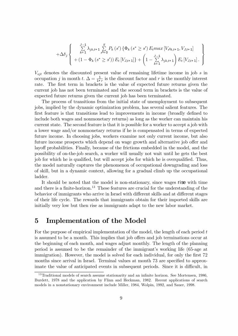
rate. The first term in brackets is the value of expected future returns given thecurrent job has not been terminated and the second term in brackets is the value ofexpected future returns given the current job has been terminated.The process of transitions from the initial state of unemployment to subsequent

jobs, implied by the dynamic optimization problem, has several salient features. Thefirst feature is that transitions lead to improvements in income (broadly defined toinclude both wages and nonmonetary returns) as long as the worker can maintain hiscurrent state. The second feature is that it is possible for a worker to accept a job witha lower wage and/or nonmonetary returns if he is compensated in terms of expectedfuture income. In choosing jobs, workers examine not only current income, but alsofuture income prospects which depend on wage growth and alternative job offer andlayoff probabilities. Finally, because of the frictions embedded in the model, and thepossibility of on-the-job search, a worker will usually not wait until he gets the bestjob for which he is qualified, but will accept jobs for which he is overqualified. Thus,the model naturally captures the phenomenon of occupational downgrading and lossof skill, but in a dynamic context, allowing for a gradual climb up the occupationalladder.It should be noted that the model is non-stationary, since wages rise with time

and there is a finite-horizon.13 These features are crucial for the understanding of thebehavior of immigrants who arrive in Israel with different skills and at different stagesof their life cycle. The rewards that immigrants obtain for their imported skills areinitially very low but then rise as immigrants adapt to the new labor market.

5 Implementation of the ModelFor the purpose of empirical implementation of the model, the length of each period tis assumed to be a month. This implies that job offers and job terminations occur atthe beginning of each month, and wages adjust monthly. The length of the planningperiod is assumed to be the remainder of the immigrant’s working life (65-age atimmigration). However, the model is solved for each individual, for only the first 72months since arrival in Israel. Terminal values at month 73 are specified to approx-imate the value of anticipated events in subsequent periods. Since it is difficult, in

13Traditional models of search assume stationarity and an infinite horizon. See Mortensen, 1986,Burdett, 1978 and the application by Flinn and Heckman, 1982. Recent applications of searchmodels in a nonstationary environment include Miller, 1984, Wolpin, 1992, and Sauer, 1998.

9

general, to find analytical solutions to dynamic programs of this type, the model issolved numerically by backward recursion, starting with the terminal value functionsin month 73.In each month, the immigrant can hold a job in one of four broad occupational

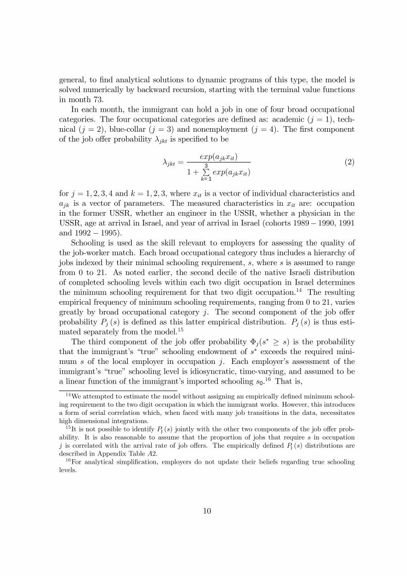
categories. The four occupational categories are defined as: academic (j = 1), tech-nical (j = 2), blue-collar (j = 3) and nonemployment (j = 4). The first componentof the job offer probability λjkt is specified to be

λjkt =exp(ajkxit)

1 +3Pk=1exp(ajkxit)

(2)

for j = 1, 2, 3, 4 and k = 1, 2, 3, where xit is a vector of individual characteristics andajk is a vector of parameters. The measured characteristics in xit are: occupationin the former USSR, whether an engineer in the USSR, whether a physician in theUSSR, age at arrival in Israel, and year of arrival in Israel (cohorts 1989− 1990, 1991and 1992− 1995).Schooling is used as the skill relevant to employers for assessing the quality of

the job-worker match. Each broad occupational category thus includes a hierarchy ofjobs indexed by their minimal schooling requirement, s, where s is assumed to rangefrom 0 to 21. As noted earlier, the second decile of the native Israeli distributionof completed schooling levels within each two digit occupation in Israel determinesthe minimum schooling requirement for that two digit occupation.14 The resultingempirical frequency of minimum schooling requirements, ranging from 0 to 21, variesgreatly by broad occupational category j. The second component of the job offerprobability Pj (s) is defined as this latter empirical distribution. Pj (s) is thus esti-mated separately from the model.15

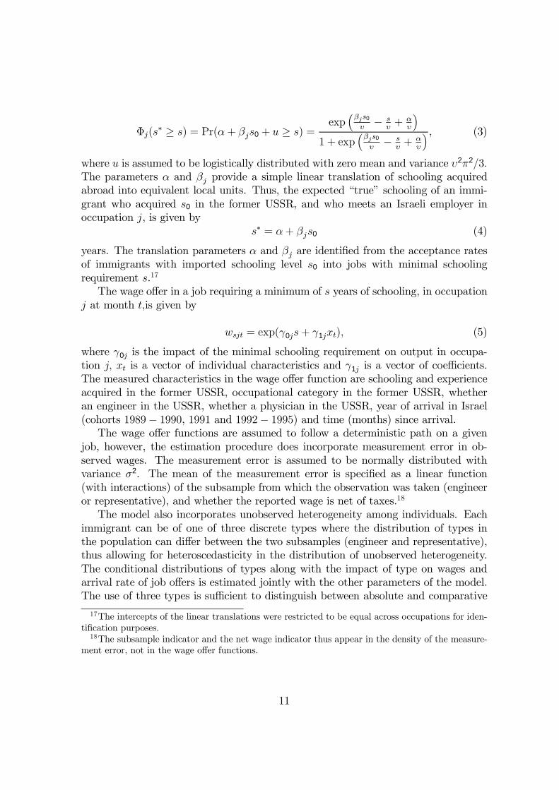
The third component of the job offer probability Φj(s∗ ≥ s) is the probabilitythat the immigrant’s “true” schooling endowment of s∗ exceeds the required mini-mum s of the local employer in occupation j. Each employer’s assessment of theimmigrant’s “true” schooling level is idiosyncratic, time-varying, and assumed to bea linear function of the immigrant’s imported schooling s0.16 That is,

14We attempted to estimate the model without assigning an empirically defined minimum school-ing requirement to the two digit occupation in which the immigrant works. However, this introducesa form of serial correlation which, when faced with many job transitions in the data, necessitateshigh dimensional integrations.15It is not possible to identify Pj(s) jointly with the other two components of the job offer prob-

ability. It is also reasonable to assume that the proportion of jobs that require s in occupationj is correlated with the arrival rate of job offers. The empirically defined Pj(s) distributions aredescribed in Appendix Table A2.16For analytical simplification, employers do not update their beliefs regarding true schooling

levels.

10

Φj(s∗ ≥ s) = Pr(α+ βjs0 + u ≥ s) =

exp³βjs0

υ− s

υ+ α

υ

´1 + exp

³βjs0

υ− s

υ+ α

υ

´ , (3)

where u is assumed to be logistically distributed with zero mean and variance υ2π2/3.The parameters α and βj provide a simple linear translation of schooling acquiredabroad into equivalent local units. Thus, the expected “true” schooling of an immi-grant who acquired s0 in the former USSR, and who meets an Israeli employer inoccupation j, is given by

s∗ = α+ βjs0 (4)

years. The translation parameters α and βj are identified from the acceptance ratesof immigrants with imported schooling level s0 into jobs with minimal schoolingrequirement s.17

The wage offer in a job requiring a minimum of s years of schooling, in occupationj at month t,is given by

wsjt = exp(γ0js+ γ1jxt), (5)

where γ0j is the impact of the minimal schooling requirement on output in occupa-tion j, xt is a vector of individual characteristics and γ1j is a vector of coefficients.The measured characteristics in the wage offer function are schooling and experienceacquired in the former USSR, occupational category in the former USSR, whetheran engineer in the USSR, whether a physician in the USSR, year of arrival in Israel(cohorts 1989− 1990, 1991 and 1992− 1995) and time (months) since arrival.The wage offer functions are assumed to follow a deterministic path on a given

job, however, the estimation procedure does incorporate measurement error in ob-served wages. The measurement error is assumed to be normally distributed withvariance σ2. The mean of the measurement error is specified as a linear function(with interactions) of the subsample from which the observation was taken (engineeror representative), and whether the reported wage is net of taxes.18

The model also incorporates unobserved heterogeneity among individuals. Eachimmigrant can be of one of three discrete types where the distribution of types inthe population can differ between the two subsamples (engineer and representative),thus allowing for heteroscedasticity in the distribution of unobserved heterogeneity.The conditional distributions of types along with the impact of type on wages andarrival rate of job offers is estimated jointly with the other parameters of the model.The use of three types is sufficient to distinguish between absolute and comparative

17The intercepts of the linear translations were restricted to be equal across occupations for iden-tification purposes.18The subsample indicator and the net wage indicator thus appear in the density of the measure-

ment error, not in the wage offer functions.

11

advantages in the unobserved ability of immigrants in different occupations.19

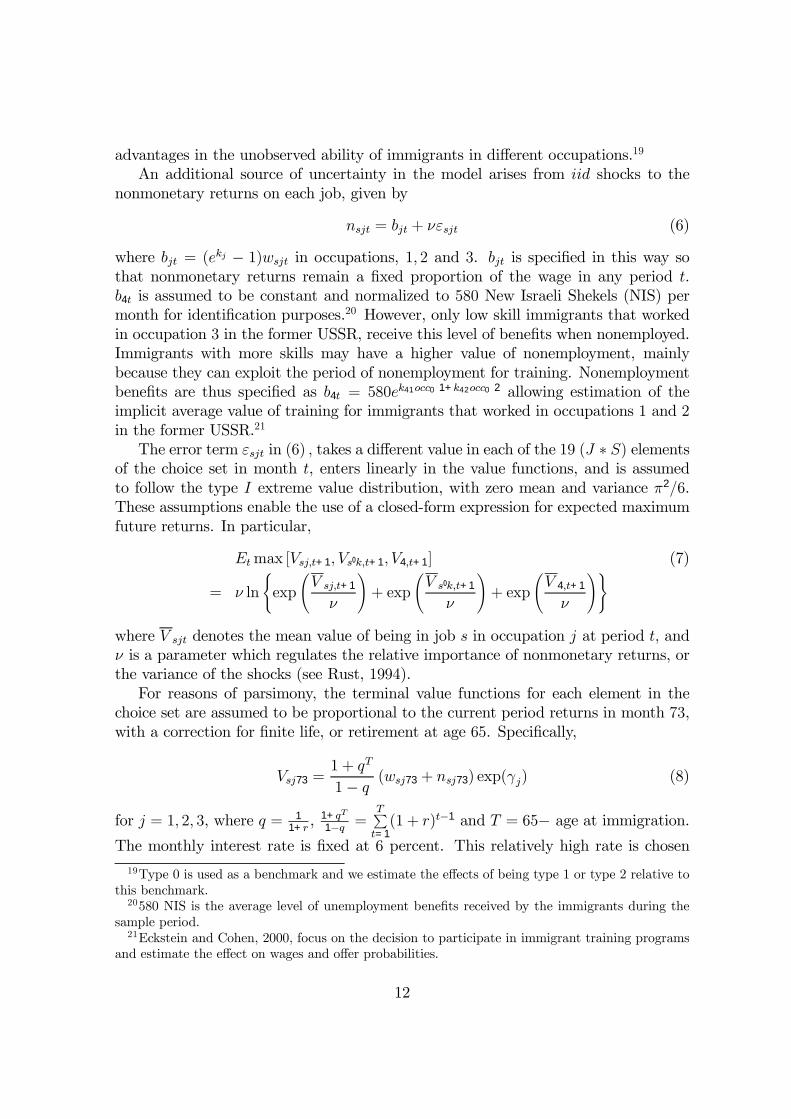
An additional source of uncertainty in the model arises from iid shocks to thenonmonetary returns on each job, given by

nsjt = bjt + νεsjt (6)

where bjt = (ekj − 1)wsjt in occupations, 1, 2 and 3. bjt is specified in this way sothat nonmonetary returns remain a fixed proportion of the wage in any period t.b4t is assumed to be constant and normalized to 580 New Israeli Shekels (NIS) permonth for identification purposes.20 However, only low skill immigrants that workedin occupation 3 in the former USSR, receive this level of benefits when nonemployed.Immigrants with more skills may have a higher value of nonemployment, mainlybecause they can exploit the period of nonemployment for training. Nonemploymentbenefits are thus specified as b4t = 580ek41occ0 1+k42occ0 2 allowing estimation of theimplicit average value of training for immigrants that worked in occupations 1 and 2in the former USSR.21

The error term εsjt in (6) , takes a different value in each of the 19 (J ∗ S) elementsof the choice set in month t, enters linearly in the value functions, and is assumedto follow the type I extreme value distribution, with zero mean and variance π2/6.These assumptions enable the use of a closed-form expression for expected maximumfuture returns. In particular,

Etmax [Vsj,t+1, Vs0k,t+1, V4,t+1] (7)

= ν ln

(exp

ÃV sj,t+1

ν

!+ exp

ÃV s0k,t+1

ν

!+ exp

ÃV 4,t+1

ν

!)

where V sjt denotes the mean value of being in job s in occupation j at period t, andν is a parameter which regulates the relative importance of nonmonetary returns, orthe variance of the shocks (see Rust, 1994).For reasons of parsimony, the terminal value functions for each element in the

choice set are assumed to be proportional to the current period returns in month 73,with a correction for finite life, or retirement at age 65. Specifically,

Vsj73 =1 + qT

1− q (wsj73 + nsj73) exp(γj) (8)

for j = 1, 2, 3, where q = 11+r, 1+qT

1−q =TPt=1(1 + r)t−1 and T = 65− age at immigration.

The monthly interest rate is fixed at 6 percent. This relatively high rate is chosen

19Type 0 is used as a benchmark and we estimate the effects of being type 1 or type 2 relative tothis benchmark.20580 NIS is the average level of unemployment benefits received by the immigrants during the

sample period.21Eckstein and Cohen, 2000, focus on the decision to participate in immigrant training programs

and estimate the effect on wages and offer probabilities.

12

to reflect the fact that immigrants had almost no initial assets and face borrowingconstraints.22 The proportionality constants γj, j = 1, 2, 3 are estimable parametersand capture the implicit value of future events.The model is estimated using full information maximum likelihood. For a given

vector of trial parameters, the dynamic program is solved by backward recursionfor each immigrant and for each unobserved type, starting with the terminal valuefunctions in month 73. Given the type-specific expected value functions for eachindividual, in every state in each month, the estimation problem is reduced to astatic panel data multinomial logit with unobserved heterogeneity. That is, given theassumptions on the shock to nonmonetary returns, the choice probabilities can becalculated according to the closed form

Pr (Vs0kt ≥ Vsjt, Vs0kt ≥ V4t) =

exp(V s0kt−V 4t

ν)

1 + exp(V sjt−V 4t

ν) + exp(V s0kt−V 4t

ν)

. (9)

Observed wages, on accepted jobs, are incorporated into estimation by multiplyingthe choice probability in month t by the measurement error density in the reportedwage. The choice probability is thus conditional on the true wage. If no wage isobserved, only the choice probability enters the type-specific likelihood contribution.The unconditional likelihood contribution of each individual is constructed by

taking a weighted average over the three type-specific likelihood contributions (seeHeckman and Singer (1984)). The weights are specified to be a (logistic) function ofthe subsample indicator. The parameters of the model are recovered by re-solving thedynamic program and re-constructing the likelihood contributions for each iterationof the optimization algorithm. The solution to the dynamic program, the inclusion ofpermanent unobserved heterogeneity and the joint estimation of the wage functionsand choice probabilities correct the wage function estimates for biases due to self-selection.23

6 ResultsThis section discusses specific parameter estimates of interest only, since there are atotal of 104 estimated parameters, and highlights the main features of the model. Theparameter estimates and their associated standard errors are presented in AppendixTable A3.24

22We attempted to estimate the interest rate along with the other parameters of the model butwere not successful. The interest rate could not be separated from the arrival rates of job offers.23The state space is small enough to enable a full solution to the dynamic program. The incor-

poration of endogenously accumulated job and/or occupation-specific work experience in the modelwould increase the size of the state space to an extent that would require approximate solutiontechniques (see Keane and Wolpin, 1994, for further discussion).24Standard errors are calculated by using numerical derivatives and the outer product approxi-

mation to the Hessian.

13

6.1 Wages

The estimated parameters of the wage offer functions show that the returns immi-grants obtain in Israel for potential work experience in the USSR are very small inoccupations 1 and 3. In occupation 2, returns are relatively higher but still small inmagnitude. In contrast, experience accumulated in Israel during the first 6 years, asproxied by time in Israel, has a substantial positive effect of .00665 per month, (8.0percent annually) in occupations 1 and 2. In occupation 3, experience accumulatedin Israel has a slightly smaller but still substantial positive effect of .00649 per month(7.8 percent annually). The impact of imported schooling on wages, on any givenjob for which schooling exceeds the minimal requirement, is negligible in occupation3, slightly negative in occupation 1 and somewhat more negative in occupation 2.However, higher imported schooling levels are associated with a higher probability ofobtaining a job with a greater minimal schooling requirement. Immigrants that findjobs with higher schooling requirements, obtain a wage increase of 3.3 percent peryear of required schooling in occupations 1 and 2, and 1.1 percent in occupation 3.The model thus captures the two main features of the wage data; increasing meanwages over time and rising inequality. The rising inequality is due to the gradualmove of immigrants with higher schooling levels into jobs that have higher minimalschooling requirements.The effects of other imported characteristics on wage offers are generally not sta-

tistically significant. The exceptions are the significant positive effect in occupation2 of having been an engineer, and the significant negative effect in of having been aphysician in occupations 1 and 3. . The results also indicate that unobserved types1 and 2 obtain substantially lower wages than unobserved type 0 in all occupations.Type 1 is penalized mainly in occupations 2 and 3, while type 2 is penalized mainlyin occupations 1 and 3.

6.2 Nonmonetary Returns

The variance component υ of nonmonetary returns is estimated to be 3267 NIS.Thus, a nonmonetary shock of one standard deviation, which under the extremevalue distribution occurs with a probability of about 13 percent, has an effect whichis approximately equal to the mean wage in the sample, 3304 NIS. This suggeststhat nonmonetary shocks can play an important role. One feature of the data whichinfluences this result is the presence of transitions, mainly within occupation 3, intojobs with lower minimal schooling requirements and lower wages.The estimates of the systematic components of nonmonetary returns, kj, j =

1, 2, 3 imply that mean nonmonetary benefits are zero for jobs in occupation 1. Inoccupation 2, nonmonetary benefits increase current period returns by 16 percent ofthe wage, and in occupation 3, nonmonetary benefits increase current period returnsby 18 percent of the wage. The estimates of mean nonmonetary returns are not

14

significantly different from zero.25 The estimate of the nonemployment benefit shifterk41 implies that immigrants that worked in occupation 1 in the former USSR valuecurrent nonemployment benefits by 45 percent more than unskilled immigrants fromoccupation 3 in the former USSR. The estimate of k42 implies that immigrants fromoccupation 2 value current nonemployment benefits by only 5.3 percent more thanunskilled immigrants. The additional benefit among skilled immigrants may reflectthe value of training programs in which many of these workers participate.26

6.3 Job Offer and Job Termination Probabilities

Table 6 presents the estimated values of λjkt, for each of the three unobserved typesof immigrants. There are large differences in these probabilities between the threeunobserved types. The estimates imply that type 0 immigrants meet substantiallymore employers in occupation 1. Type 1 immigrants meet very few employers outsideof occupation 3. Type 2 immigrants meet more employers in occupation 3 than bothtype 0 and type 1 immigrants.The table also shows that λjkt is generally higher when in nonemployment. For

example, the probability of meeting an employer in occupation 1 is higher fromnonemployment than from jobs in occupation 3 and occupation 2, for all types³bλ41t > bλ31t > bλ21t

´. However, being already employed in occupation 1 and being

in nonemployment yield similar estimated probabilities³bλ41t

∼= bλ11t

´. An exception

to this latter pattern occurs when employed in occupation 3. The probability ofmeeting an employer in occupation 3 is higher in nonemployment.The estimated values of λ41t for types 0, 1 and 2 are .032, .002 and .011, respec-

tively. The estimated values of λ43t are much higher, .129, .029 and .165 for thethree types, respectively. Thus, from nonemployment, a type 0 immigrant’s expectedwaiting time to meet an employer in occupation 1 is 29 months, while his expectedwaiting time to meet an employer in occupation 3 is only 8 months. These estimatesreflect the market conditions that immigrants face upon entry. It is much easier forthem to find jobs as unskilled workers.Based on the estimated parameters of λjkt, it is further noted that older individ-

uals, and those who arrived in Israel in later years, have lower probabilities to meetemployers in occupations 1 and 2. This reflects possible changes in cohort quality and“congestion” effects in Israel. As expected, the occupational category in the formerUSSR is an important signal for Israeli employers. Immigrants that worked in occu-pation 1 in the former USSR meet substantially more employers in occupation 1 in

25This is due to correlation with the terminal value parameters, which also influence the value ofa job within the sample period. The terminal value parameters, however, are highly significant.26Approximately 60 percent of skilled male immigrants (immigrants from occupations 1 and 2 in

the former USSR) participate in job training programs, for 6 months on average. Job training isprovided by the government and is conditioned on a prior course in Hebrew language proficiency,lasting 4 months on average. See Eckstein and Cohen, 2000.

15

Israel. In comparison to all others that worked in occupation 1 in the former USSR,engineers meet fewer employers in occupation 1 while physicians meet more.The estimated coefficient for Φj(s∗ ≥ s), the probability of being accepted to a job

having already met an employer, yield the following quality adjustment for importedschooling

s∗1 = 10.072 + .456s0

s∗2 = 10.072 + .270s0 (10)

s∗3 = 10.072 + .080s0.

The marginal effects of imported schooling are thus .456 in occupation 1, .270 inoccupation 2 and .080 in occupation 3. The corresponding “break even” levels are19, 14 and 11 years of schooling , in occupations 1, 2 and 3, respectively. For com-parability with Israelis, imported schooling is adjusted downwards (upwards) if it isabove (below) the break even level.The acceptance probabilities, which depend also on the estimated variances, are

displayed in Figure 1. In occupation 1, immigrants are accepted with probabilityclose to 1 to jobs that require less than their imported schooling, s0. They arealso accepted with a positive probability into jobs requiring slightly more schoolingthan they posses. For example, an immigrant with 15 years of imported schoolingis accepted with probabilities of .909, .451 and .063 to jobs requiring 16, 17 and 18years of schooling, respectively.These results reflect the fact that, in the former USSR, one could become an

engineer (physician) by going to elementary and high school for 10 years, followedby 5 (6) years of university training. Immigrants that find jobs in occupation 1 asdoctors or engineers, are treated as if they have schooling comparable to Israelis,that is, 16 (18) years of schooling. In occupation 3, practically everyone is acceptedto jobs requiring 10 years or less, but the best jobs in this occupation, requiring 12years of schooling, are generally not available to immigrants, even with a high levelof schooling. Similarly, immigrants with a high level of schooling have only a smallprobability to be accepted into jobs requiring 16 years of schooling in occupation 2.Stated differently, immigrants have a lower probability than Israelis to receive the topoffers in occupations 2 and 3.The model also allows for involuntary separations due to job termination. The

estimates of δj are .0035 .0081 and .0052 in occupations, 1, 2 and 3, respectively.The termination probability estimates are small but highly significant. The estimatesimply that immigrants can hold on to their jobs for long periods of time (24, 10 and16 years, respectively) unless they decide to quit.

6.4 Choice Probabilities and Types

Table 7 presents the predicted occupational choice distribution by unobserved type forselected months after immigration. The choice frequencies are calculated by drawing

16

from the distributions of the random elements of the model, simulating choice historiesfor each individual 10, 000 times, and averaging over all simulations and individuals.The figures show that the proportion of each type of immigrant in occupation 1

grows over time but that there is a much higher proportion of type 0 immigrantsin this occupation in each month. Moreover, the proportion of type 0 immigrants inoccupation 1 increases at a much faster rate. The proportion of each type of immigrantin occupation 2 is also nondecreasing. Type 2 immigrants have the highest proportionin occupation 2 as well as the fastest rate of increase. In occupation 3, the proportionof each type of immigrant rises to a peak and subsequently falls. The peak occursearlier for type 0 and type 2 immigrants. In nonemployment, the proportion of type1 immigrants is clearly the highest. Nonemployment falls sharply for types 0 and 2and only gradually for type 1 immigrants.The choice frequency patterns in Table 7 can be explained by the fact that a

nonemployed type 0 immigrant accepts almost any job offer in the early months afterarrival. However, as his occupational status in Israel improves, he accepts feweroffers outside of occupation 1. A type 1 immigrant is reluctant to accept offers fromoccupation 3 in which his wage penalty is highest. A type 1 immigrant waits for offersin occupation 1, but these offers arrive with a very low frequency. In contrast, a type2 immigrant accepts offers mainly from occupation 2 in which his wage penalty is thelowest.Based on the sign patterns of the estimated parameters in the wage offer functions

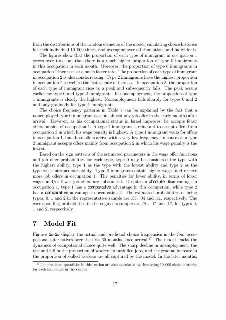
and job offer probabilities for each type, type 0 may be considered the type withthe highest ability, type 1 as the type with the lowest ability and type 2 as thetype with intermediate ability. Type 0 immigrants obtain higher wages and receivemore job offers in occupation 1. The penalties for lower ability, in terms of lowerwages and/or fewer job offers are substantial. Despite an absolute disadvantage inoccupation 1, type 1 has a comparative advantage in this occupation, while type 2has a comparative advantage in occupation 2. The estimated probabilities of beingtypes, 0, 1 and 2 in the representative sample are .55, .04 and .41, respectively. Thecorresponding probabilities in the engineers sample are .76, .07 and .17, for types 0,1 and 2, respectively.

7 Model FitFigures 2a-2d display the actual and predicted choice frequencies in the four occu-pational alternatives over the first 60 months since arrival.27 The model tracks thedynamics of occupational choice quite well. The sharp decline in unemployment, therise and fall in the proportion of workers in unskilled jobs, and the gradual increase inthe proportion of skilled workers are all captured by the model. In the later months,

27The predicted quantities in this section are also calculated by simulating 10, 000 choice historiesfor each individual in the sample.

17

in which there are fewer observations, there is a mild underprediction of the propor-tion in occupation 1 and an overprediction of the proportion in occupation 3. On thebasis of a chi-square test which compares the actual and predicted choice distributionsin each month, the hypothesis of identical actual and predicted choice distributionsis not rejected in 54 out of 72 months.28

Table 8 presents the actual and predicted monthly transitions across occupations,averaged over the sample period. The fit is quite good. On the basis of a chi-square test, the hypothesis that the actual and predicted transition matrices areidentical is not rejected. The matrix shows that entry into occupation 1 occursmost often from nonemployment. Workers in occupations 2 and 3 enter occupation 1indirectly, through nonemployment. Voluntary transitions into nonemployment occurwhen there are large random shocks to nonmonetary returns. However, these shocksmainly influence mismatches, i.e., type 2 immigrants that work in occupation 1 andtype 1 immigrants that work in occupation 3. These movements also reflect, in part,participation in training programs.The model is also capable of capturing the time patterns in transitions during the

sample period. In Figures 3a and 3b, the actual and predicted transition rates betweenemployment and nonemployment during the first 60 months are displayed. The modelreproduces the decline in the exit rate from nonemployment and the decline in there-entry rate into nonemployment without reliance on time effects in the arrival rateof job offers. The decline in the re-entry rate into nonemployment occurs as wagesrise sharply over time. The opportunity cost of voluntarily separating and searchingefficiently in nonemployment rises, thus discouraging these types of transitions. Thedecline in the exit rate from nonemployment is explained by the changing mix ofunobserved types in the population of the nonemployed over time. Type 0 and type 2immigrants constitute the majority of the nonemployed in the early months and theseimmigrants have relatively high exit rates. In the later months, the population of thenonemployed consists mainly of type 1 immigrants. Type 1 immigrants have very pooremployment prospects and thus low exit rates from nonemployment. On the basisof a chi-square test in each month, the hypothesis of identical actual and predictedexit rates from nonemployment is not rejected in 66 out of 72 months. Similarly, thehypothesis of identical actual and predicted entry rates into nonemployment is notrejected in 68 out of 72 months.Table 9 presents the actual and predicted mean accepted wages in each occupation-

job category in which there are wage observations. As shown in the table, predictedwages track observed wages quite well for the cells in which there are a substantialnumber of wage observations. Examining the fit for all immigrants with wages, thesimple correlations between actual and predicted wages is .602 in logs. Althoughthe maximum likelihood estimation adjusts the coefficients of the wage functions tofit both wages and occupational choices, it yields a wage fit that exceeds the fit of

28The chi-square statistics are not adjusted for the fact that the parameters of the model havebeen estimated. Rejection of the null hypothesis is at the 5 percent level of significance.

18

a reduced form log-linear regression of wages on the same exogenous variables thatappear in the structural model (.519 in logs). For comparison purposes the predictedvalues from the second OLS regression specification in Table 5, which includes theendogenous job choice variables, are also displayed.29

Table 9 also reveals large differences in predicted wages by type. A type 1 im-migrant earns very low wages in occupation 3, while his wages in occupation 1, inthe rare case that he finds a job in occupation 1, are substantially higher. A type 2immigrant obtains the highest wages in occupation 2. A type 0 immigrant obtainsthe highest wages in occupation 1.Table 10 illustrates the impact of job transitions on wage growth. Employed

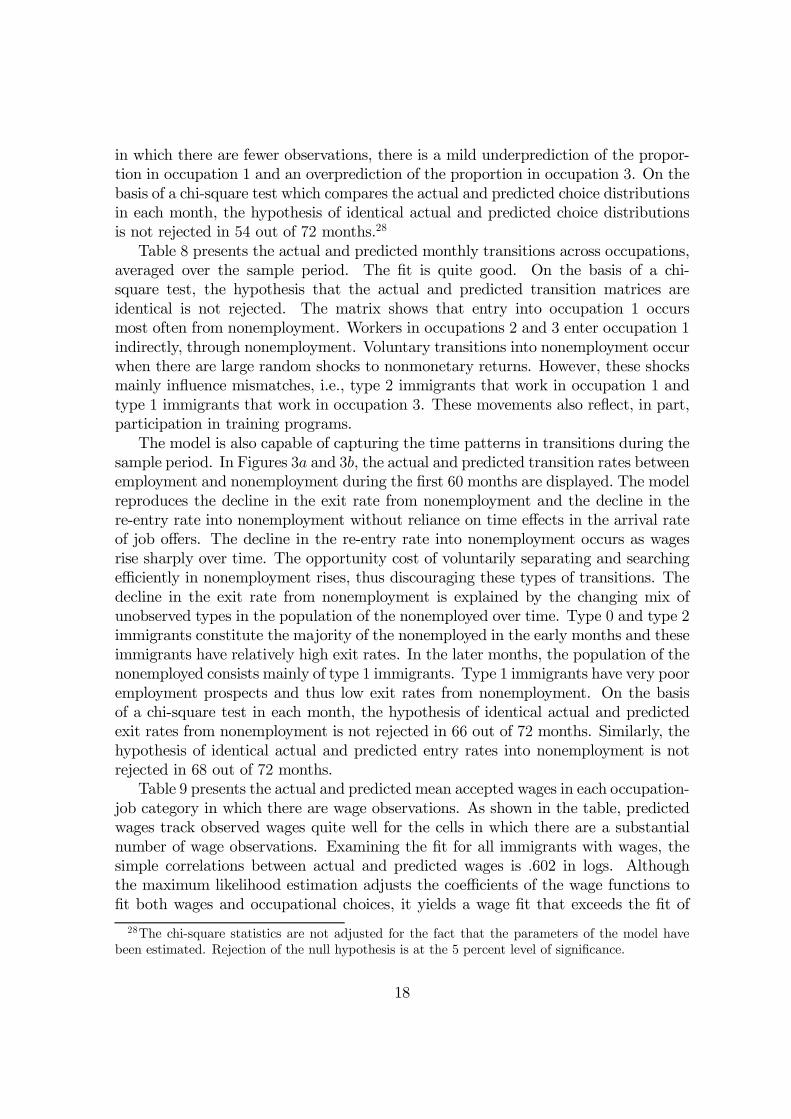
workers are classified into stayers and movers. Stayers are immigrants that do notchange their job from period t to period t + 1. Movers, from period t to periodt + 1, are subdivided into job changers within and across occupations. The tablepresents the actual and simulated proportions of such transitions and the associatedpredicted wage changes30, averaged over individuals and sample months. The modelmimics the sample proportions of movers and stayers quite well. The predicted wagegrowth among stayers is a weighted average of the estimated monthly wage growthparameters in occupations 1, 2 and 3. Movers within occupations have a predictedaverage monthly wage growth of 2 percent and movers across occupations have asubstantial average wage growth of 18.3 percent. The predicted impact of job changeson wage growth is thus quite large. However, such switches are rare and occur in only1.1 percent of the time periods. The majority of transitions are to nonemploymentand from nonemployment. Ignoring the impact of these latter transitions on wages,which occur 25.6 percent of the time, the average annual growth rate in wages foremployed workers is 8.82 percent a year. Approximately 18 percent of the annual wagegrowth (1.32 percentage points) can be attributed to job switches. These results aresimilar to the reduced form estimates, based on pooled cross section data for theperiod 1991 − 1995, presented in Eckstein and Weiss, 1998. In this latter study, 17percent (1.13 percentage points) of a predicted annual wage growth of 6.71 percentcan be attributed to occupational switches. Among immigrants with 16+ years ofschooling, 17 percent (1.44 percentage points) of a predicted annual wage growthof 8.28% can be attributed to occupational switches. Apart from the differences inthe samples, the main methodological difference in the study presented here is thatoccupational switches are endogenously determined.

29The OLS regression is similar but not identical to the wage functions estimated in the model.For example, the regression is not estimated separately for each occupation and does not includecontrols for unobserved heterogeneity. The corresponding measure of fit is .592 in logs.30The data on wages in the sample is very sparse and there are no observations of wage changes

among stayers or movers in adjacent months. Therefore, we cannot present the corresponding actualwage changes.

19

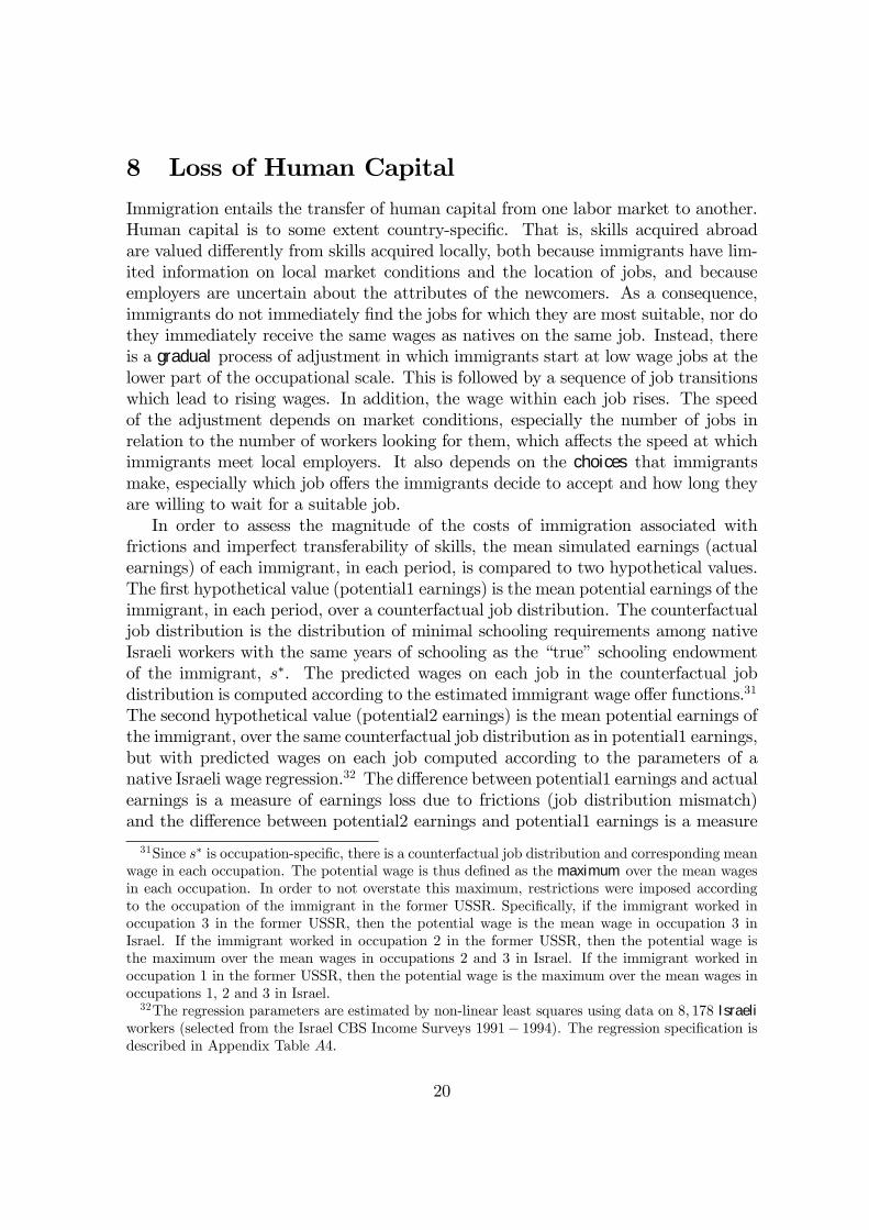
8 Loss of Human CapitalImmigration entails the transfer of human capital from one labor market to another.Human capital is to some extent country-specific. That is, skills acquired abroadare valued differently from skills acquired locally, both because immigrants have lim-ited information on local market conditions and the location of jobs, and becauseemployers are uncertain about the attributes of the newcomers. As a consequence,immigrants do not immediately find the jobs for which they are most suitable, nor dothey immediately receive the same wages as natives on the same job. Instead, thereis a gradual process of adjustment in which immigrants start at low wage jobs at thelower part of the occupational scale. This is followed by a sequence of job transitionswhich lead to rising wages. In addition, the wage within each job rises. The speedof the adjustment depends on market conditions, especially the number of jobs inrelation to the number of workers looking for them, which affects the speed at whichimmigrants meet local employers. It also depends on the choices that immigrantsmake, especially which job offers the immigrants decide to accept and how long theyare willing to wait for a suitable job.In order to assess the magnitude of the costs of immigration associated with

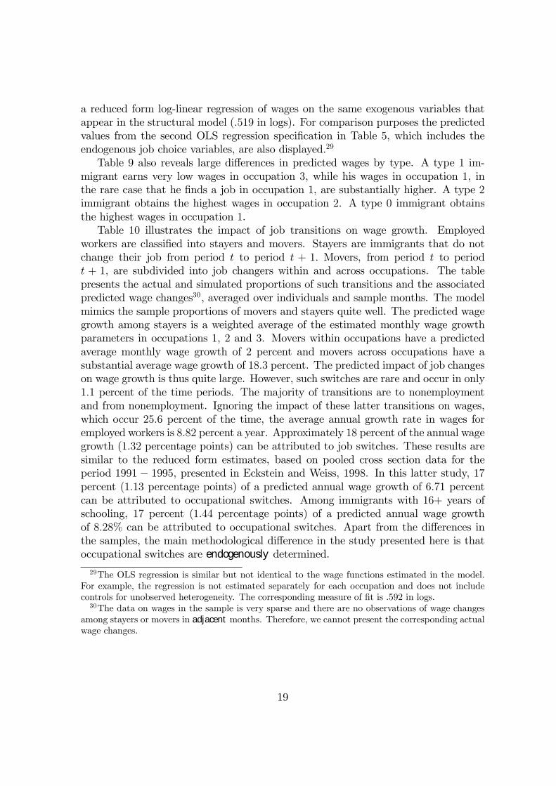
frictions and imperfect transferability of skills, the mean simulated earnings (actualearnings) of each immigrant, in each period, is compared to two hypothetical values.The first hypothetical value (potential1 earnings) is the mean potential earnings of theimmigrant, in each period, over a counterfactual job distribution. The counterfactualjob distribution is the distribution of minimal schooling requirements among nativeIsraeli workers with the same years of schooling as the “true” schooling endowmentof the immigrant, s∗. The predicted wages on each job in the counterfactual jobdistribution is computed according to the estimated immigrant wage offer functions.31

The second hypothetical value (potential2 earnings) is the mean potential earnings ofthe immigrant, over the same counterfactual job distribution as in potential1 earnings,but with predicted wages on each job computed according to the parameters of anative Israeli wage regression.32 The difference between potential1 earnings and actualearnings is a measure of earnings loss due to frictions (job distribution mismatch)and the difference between potential2 earnings and potential1 earnings is a measure

31Since s∗ is occupation-specific, there is a counterfactual job distribution and corresponding meanwage in each occupation. The potential wage is thus defined as the maximum over the mean wagesin each occupation. In order to not overstate this maximum, restrictions were imposed accordingto the occupation of the immigrant in the former USSR. Specifically, if the immigrant worked inoccupation 3 in the former USSR, then the potential wage is the mean wage in occupation 3 inIsrael. If the immigrant worked in occupation 2 in the former USSR, then the potential wage isthe maximum over the mean wages in occupations 2 and 3 in Israel. If the immigrant worked inoccupation 1 in the former USSR, then the potential wage is the maximum over the mean wages inoccupations 1, 2 and 3 in Israel.32The regression parameters are estimated by non-linear least squares using data on 8, 178 Israeli

workers (selected from the Israel CBS Income Surveys 1991− 1994). The regression specification isdescribed in Appendix Table A4.

20

of earnings loss due to a lower market valuation of imported skills.For the purpose of assessing long-run outcomes, the actual and potential earnings

of each immigrant are computed from the age at arrival until retirement at age 65. Inorder to calculate actual and potential earnings past month 72 in Israel (the horizon ofthe model) in a computationally practical way, a period length of one year is assumedin the simulation of the model beyond month 72. Further, since it is not possible toidentify quadratic effects on wage growth within the sample period, and thus reliablypredict wage offers beyond month 72, the wage offer functions in the yearly model arereplaced by wage functions estimated separately, using data on the annual earningsof previous waves of immigrants from the Soviet Union.33 However, the importedwage functions in the yearly model do not contaminate the simulated job choicesin months. That is, the monthly model and the yearly model are disconnected byseparate backward recursions. The backward recursion and subsequent simulationof the monthly model uses the terminal value functions, as in estimation.34 Theestimated monthly wage offer functions do, however, influence job choices in theyearly model. The ratio of the wage offer in each job in month 73, according theestimated monthly model, to the wage offer in each job in month 73, according tothe out-of-sample regression, is used to adjust the yearly wage offers. Let this ratiobe denoted by

wmsj73

wysj73. The yearly wage offers in each job, in each year, is multiplied by

wmsj73

wysj73.35

Figure 4a displays the time paths of simulated actual and potential earnings, aver-aged over immigrants that worked in occupation 1 in the former USSR and that were40 years old or younger on arrival. Figure 4b displays the corresponding time pathsfor immigrants that were older than 40 on arrival. The simulated actual earnings ofimmigrants are always below their simulated potential earnings, but the gap closeswith the duration of time in Israel. The change over time in potential2 earnings isdriven by the immigrants’ increase in local work experience, where the impact of totalwork experience (imported plus local) is evaluated using the native Israeli regression

33The regression specification, which is similar to that in Eckstein and Weiss 1998, is described inAppendix Table A4. In the out of sample predictions there are no pure time effects. The growth inwages is attributed to accumulation of experience and rising prices of imported skills.34It is interesting to note that connecting the monthly and yearly models by a full backward

recursion starting from age 65, does not substantially change the simulation results. The terminalvalue functions estimated in the model are thus consistent with the value functions generated usingthe imported wage functions.35Estimated monthly job offer probabilities are also transformed into yearly equivalents. Let q

be the probability of meeting an employer in a particular month where q = 1 − λj1t − λj2t − λj3t.The probability that the person will meet an employer in occupation k once during the year (i.e.,

in one of n months) is λjkt

£1 + q + q2 + · · ·+ qn−1

¤= λjkt

h1−qn

1−q

iThe probability that the person

will receive no offer is qn. Clearly, λj1t

h1−qn

1−q

i+ λj2t

h1−qn

1−q

i+ λj3t

h1−qn

1−q

i+ qn = 1, since q =

1−λj1t−λj2t−λj3t. The other two components of the job offer probability, Pj (s) and Φj(s∗ ≥ s),

are not dependent on the length of the period.

21

coefficients. The sharp rise in potential1 earnings reflects the higher return that im-migrants obtain for local work experience using the coefficients of the immigrant wagefunctions. The higher return is mainly due to rising returns to imported skills andcomplementarity between local and imported human capital (see Eckstein and Weiss,1998). The even sharper rise in simulated actual earnings occurs as the distributionof jobs that immigrants hold changes over time. That is, the strong wage growth isaccompanied by a movement into higher paying jobs and occupations.There are marked differences in the time paths of actual and potential earnings

between the two age groups. Younger immigrants initially earn half of their potential,but gradually close the gap. After 25 years in Israel, younger immigrants earn 70percent of what they would have earned as native Israelis. The gap in earnings inyear 25 is evenly divided between job distribution mismatch and a lower marketvaluation of imported skills. Immigrants that arrived at an older age initially earnthe same as younger immigrants, but these earnings constitute only a third of theirpotential, indicating negligible initial returns to imported work experience. As timesince immigration advances, the rewards for imported skills rise for both younger andolder immigrants, but the occupational status of older immigrants is substantiallylower. Older immigrants remain locked in low skill occupations. After 10 years inIsrael, older immigrants earn only half as much as comparable native Israelis. Thedifferent rates of occupational upgrading by age at arrival are shown in Table 11.Among immigrants that worked in occupation 1 in the former USSR and that were40 years old or less on arrival, 60 percent are predicted to be employed in occupation1 in Israel, 25 years after immigration. This is compared to 75 percent among similarimmigrants from the USSR that arrived in Israel during the 1970s (see Eckstein andWeiss, 1998).Because of the sharp changes in earnings with time in Israel and the endogeneity

of wages and jobs, whereby currently low wages may be traded for higher wages in thefuture, the appropriate summary statistic of earnings loss is the difference in the ex-pected discounted present value of actual and potential earnings over the immigrantsremaining working life. Table 12 describes the main findings for this summary mea-sure.36 The estimated lifetime earnings loss (potential2-actual) is 253, 200 US Dollars.This loss constitutes 57 percent of the lifetime earnings that these immigrants wouldhave obtained had they been native Israelis with the same measured attributes. Theestimated lifetime loss is thus quite substantial.Most of the loss, 190, 900 US Dollars, can be attributed to the fact that immigrants

are paid lower wages than Israelis on the same jobs, especially in the early years afterarrival. This loss constitutes 43 percent of total potential lifetime earnings. Thelifetime loss of earnings due to frictions in the labor market (nonemployment and jobdistribution mismatch) is 62, 300 US Dollars, which constitutes 14 percent of totalpotential lifetime earnings.

36In the calculation of discounted lifetime earnings, zeros are included when the immigrant issimulated to be in nonemployment.

22

The estimated lifetime earnings loss varies substantially among immigrants. Im-migrants with more schooling tend to have higher total losses. Given the strongcorrelation between schooling levels and occupation, immigrants who worked in oc-cupations 1 and 2 in the former USSR also suffer higher total losses. The figuresshow that physicians have higher losses than engineers, older immigrants have higherlosses than younger immigrants, losses increase with later arrival cohorts and type 1immigrants suffer exceedingly large losses.In order to gauge the relative importance of job distribution mismatch and a lower

market valuation of imported skills, the table decomposes the total loss into the lossdue to frictions and the loss due to prices. The estimates indicate that the loss dueto prices is, generally, far more important. This is mainly due to the lower returnsto imported schooling.37 The difference between the loss due to frictions and theloss due to prices is greatest for physicians. Immigrants that were physicians in theUSSR obtain jobs in the medical profession rather quickly in Israel but earn muchlower wages than native physicians.38 The smallest difference between the loss dueto frictions and the loss due to prices is for engineers and type 1 immigrants. Thelarge number of immigrants with engineering degrees nearly doubled the total stockof engineers in Israel. This group thus faces special difficulties obtaining engineeringjobs in the Israeli labor market. Type 1 immigrants suffer a relatively large loss due tofrictions since they constitute the permanently nonemployed. It should be noted thatthere is a discontinuity in the ranking of relative losses due to prices over schoolinglevels and occupations. Immigrants with 13-14 years suffer higher relative losses dueto prices than immigrants with 15 years of schooling. Correspondingly, immigrantsthat worked in occupation 2 in the former USSR suffer higher relative losses due toprices than immigrants that worked in occupation 1 in the former USSR. This resultis due to the relatively lower actual earnings of this group of immigrants in occupation3, the occupation in which many of these immigrants find employment.The lifetime earnings loss calculations aim at estimating the social loss of output

to the receiving country associated with the movement of human capital across labormarkets. For this reason, the loss calculations do not include the benefits that im-migrants receive when nonemployed nor the monetary value of nonmonetary benefitswhen employed. Further, the wages of Israelis are used as a benchmark. Althoughthe model contains an equivalence scale that transforms the schooling of immigrantsto local schooling, there may still be unaccounted for differences in the quality ofschooling acquired locally and abroad. Moreover, the counterfactual exercises do notaccount for possible macro effects on the Israeli labor market and wage structure.For these reasons, the potential earnings of the recent immigrants may be overstatedwhen they are attributed the current earnings of Israelis with the same observable

37Other studies have also found a higher rate of return for locally acquired schooling, see Ecksteinand Weiss, 1998, and Friedberg, 1999).38The national health system considerably expanded in the wake of the mass immigration from

the former USSR.

23

characteristics. Therefore, the estimated losses among the different groups are anupper bound on actual losses. Biases in the separately estimated immigrant and Is-raeli wage functions, due to sample selection and/or unmeasured characteristics, alsoreduce the accuracy of our estimates. We thus have more confidence in the rankingof the losses across groups of immigrants with different attributes than in the actualmagnitude of the loss.Recall that the model assumes a high annual real discount rate of 6 percent to

capture the borrowing constraint facing immigrants that came to Israel with no assets.This fact should not prevent the use of an appropriate “social” discount rate toevaluate the social loss associated with immigration. As displayed in the last tworows of Table 12, the relative losses are only slightly affected by using an annualreal discount rate of 3 percent to evaluate the discounted present value. Clearly, ifimmigrants had better access to the capital market and had faced an interest rate of3 percent, there would have been a marked effect on their choices and the estimatedparameters of the model.

9 ConclusionThis paper examines the process of entry of highly skilled immigrants into the Israelilabor market, using panel data on several cohorts of recent immigrants from theformer USSR. The main emphasis in the paper is on the occupational choices ofimmigrants that arrive with different skills and at different points in their life-cycle.This study does not investigate the reasons for wage growth within occupations andjobs, but explicitly models how immigrants adjust their choices to the expected risein their wages with the passage of time.As has been demonstrated, a simple on-the-job search model, cast as a finite-

horizon discrete choice dynamic programming problem under uncertainty, capturesquite well the observed dynamics of occupational choice during the first six years inIsrael. The dynamics consist of a speedy entry into the labor force, an initial phaseof work at low skill occupations, followed by a gradual occupational upgrading. Themodel explains the changing proportions of immigrants working in different occupa-tions in Israel without relying on time effects in job offer probabilities. The sharpincrease in the proportion of immigrants working in low skill jobs is due to the will-ingness of immigrants with high schooling levels and previous work experience in highskill occupations in the USSR, to work in low skill jobs in Israel. The subsequentdecrease in the proportion working in low skill jobs is due to the gradual transitionsof these highly skilled immigrants to jobs in high skill occupations. Permanent un-observed heterogeneity among immigrants is shown to be important in explainingthe observed declining exit rates from nonemployment. Immigrants with high exitrates from nonemployment constitute the majority without jobs in the early monthsafter immigration. As these immigrants leave nonemployment, the population ofthe nonemployed is increasingly made up of immigrants with very poor employment

24

prospects. The model is also capable of explaining the declining re-entry rates intononemployment. Nonemployment re-entry rates decline over time as wage growth onthe job raises the opportunity cost of searching efficiently for better job opportunitiesfrom nonemployment.The estimated parameters of the behavioral model, together with information on

the wages of immigrants from earlier waves, are used to examine the speed of wageconvergence between immigrants and natives. The simulation of an occupational pathand associated wages for each immigrant upon arrival to the host country and untilretirement, suggests that the earnings of recently arrived immigrants will slowly ap-proach the earnings of comparable natives. However, the sharp growth in earnings,combined with the heterogeneity in age at entry, suggest the use of the discountedpresent value of lifetime earnings as a better summary measure of economic perfor-mance in the new country. The lifetime earnings predicted by the model are thuscompared to the hypothetical lifetime earnings that immigrants would have obtainedhad their imported observable skills been valued, from the time of arrival, in the sameway as comparable natives with the same labor market experience and schooling. Theresults indicate a large gap between actual and potential lifetime earnings measures.On average, immigrants from the former USSR to Israel can expect lifetime earningsto fall short of the lifetime earnings of comparable natives by 57 percent. Of thisfigure, 14 percentage points reflect frictions associated with nonemployment and jobdistribution mismatch, and 43 percentage points reflect the gradual adaptation ofschooling and experience imported from the former USSR to the Israeli labor market.Our interpretation of these findings is that, because of lack of information by

employers on the quality of newly arrived immigrants, and by immigrants of their op-portunities in the new labor market, and because of the need for complementary localcapital (such as, language, social connections and familiarity with local institutions),there is, necessarily, a gradual process of adjustment and adaptation. The speed ofadjustment depends on market conditions and the choices made by the immigrants,which interact in a complicated way. It is not clear whether, and to what extent, thereare market failures in this process and whether there is some policy that could reducethe social loss. It is possible that limited borrowing capacity prevents immigrantsfrom making the required local investment in on the job training, which should bethe main vehicle for the acquisition of local general human capital. There is, however,no way to ascertain the quantitative importance of this latter consideration.

25

References[1] Altonji, J. and Card, D. (1991), ”The Effects of Immigration on the Labor Mar-

ket Outcomes of Less-Skilled Natives,” in J. Abowd and R. Freeman (eds.), Im-migration, Trade and the Labor Market, Chicago: University of ChicagoPress.

[2] Borjas, G. (1994), ”The Economics of Immigration,” Journal of EconomicLiterature, 32, 1667-1717.

[3] Burdett, K. (1978), “Job Search and Quit Rates,” American Economic Re-view, 68, 212-220.

[4] Card, D. (1999), ”Immigrants Inflows, Native Outflows, and the Labor MarketImpacts of Higher Immigration,”Journal of Labor Economics, forthcoming.

[5] Carrington, W. and A. Zaman (1994), “Inter-Industry Variation in the Costs ofJob Displacement,” Journal of Labor Economics, 12, 243-275.

[6] Chiswick, B. (1978), ”The Effect of Americanization on the Earnings of Foreign-Born Men,” Journal of Political Economy, 86, 897-922.

[7] Chiswick, B. (1998), ”Hebrew Language Usage: Determinants and Effects onEarnings among Immigrants in Israel,” Journal of Population Economics,11(2), 253-71.

[8] Eckstein, Z. and S. Cohen (2000), “Training and Occupational Choice,” unpub-lished manuscript.

[9] Eckstein, Z. and Y. Weiss (1998), “The Absorption of Highly Skilled Immigrants:Israel 1990-1995,” Foerder Institute Working Paper 3-98.

[10] Flinn, C. and J. Heckman (1982), “Newmethods for Analyzing Structural Modelsof Labor Force Dynamics,” Journal of Econometrics, 18, 115-168.

[11] Flug, K., Kasir, N. and G. Ofer (1992), “The Absorption of Soviet Immigrantsinto the Labor Market from 1990 Onwards: Aspects of Occupational Substitutionand Retention,” Bank of Israel Discussion Paper No. 9213.

[12] Friedberg, R. (1999), ”The Impact of Mass Migration on the Israeli Labor Mar-ket,” Quarterly Journal of Economics, forthcoming

[13] Friedberg, R. (2000), “You Can’t, Take it With You? Immigration Assimila-tion and the Portability of Human Capital: Evidence From Israel,” Journal ofLabor Economics, 18, 221-250.

26

[14] Green, D. (1999), ”Immigrant Occupational Attainment: Assimilation and Mo-bility over Time,” Journal of Labor Economics, 17, 49-79.

[15] Jacobson, L., LaLonde, R. and D. Sullivan (1993), “Earning Losses of DisplacedWorkers,” American Economic Review, 83, 685-709.

[16] Keane, M.P., and K.I. Wolpin, (1994), “The Solution and Estimation of DiscreteChoice Dynamic Programming Models by Simulation and Interpolation: MonteCarlo Evidence,” Review of Economics and Statistics, 17, 648-672.

[17] LaLonde, R. and R.Topel (1997), “Economic Impact of International Migrationand the Performance of Migrants,” in O. Stark and M. Rosenzweig (eds.)Hand-book of Population and Family Economics, Amsterdam: Elsevier.

[18] Miller, R. (1984), “Job Matching and Occupational Choice,” Journal of Polit-ical Economy, 92, 1086-1120.

[19] Mortensen, D. (1986), “Job Search and Labor Market Analysis,” in: Ashenfelter,O. and R. Layard (ed.) Handbook of Labor Economics, North Holland,Amsterdam.

[20] Neal, D. (1995), ”Industry Specific Human Capital: Evidence from DisplacedWorkers” Journal of Labor Economics, 13, 653-677.

[21] Reder, M. (1957), Labor in a Growing Economy, Wiley, New York.

[22] Rust, J. (1994), Structural Estimation of Markov Decision Problems,” in R. En-gle and D. McFadden (eds.)Handbook of Econometrics, Vol. 4, Amsterdam:Elsevier.

[23] Sauer, R. M. (1998), ”Job Mobility and the Market for Lawyers,” Journal ofPolitical Economy, 106, 147-171.

[24] Sicherman, N. (1991), “Over Education in the Labor Market,” Journal of La-bor Economics, 9, 101-122.

[25] Sussman, Z. and D. Zakai (1998), ”The Mass Immigration to of Physicians toIsrael and the Steep Rise in Wages of Veterans in Israel: A Paradox?” ResearchDepartment, Bank of Israel.

[26] Wolpin, K. (1992), “The Determinants of Black White Differences in Early Em-ployment Careers: Search, Layoffs, Quits and Endogenous Wage Growth,” Jour-nal of Political Economy, 100, 535-560.

27

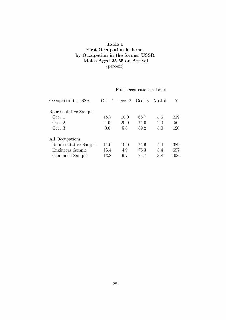
Table 1First Occupation in Israel

by Occupation in the former USSRMales Aged 25-55 on Arrival

(percent)

First Occupation in Israel

Occupation in USSR Occ. 1 Occ. 2 Occ. 3 No Job N

Representative SampleOcc. 1 18.7 10.0 66.7 4.6 219Occ. 2 4.0 20.0 74.0 2.0 50Occ. 3 0.0 5.8 89.2 5.0 120

All OccupationsRepresentative Sample 11.0 10.0 74.6 4.4 389Engineers Sample 15.4 4.9 76.3 3.4 697Combined Sample 13.8 6.7 75.7 3.8 1086

28

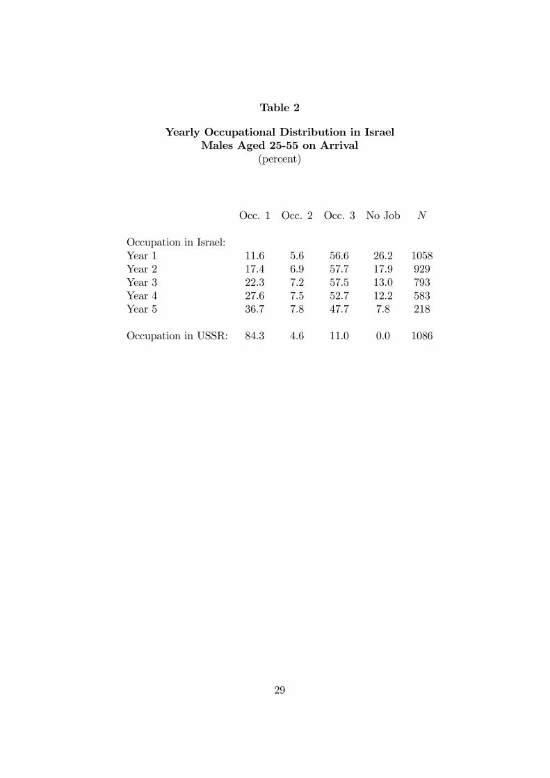
Table 2

Yearly Occupational Distribution in IsraelMales Aged 25-55 on Arrival

(percent)

Occ. 1 Occ. 2 Occ. 3 No Job N

Occupation in Israel:Year 1 11.6 5.6 56.6 26.2 1058Year 2 17.4 6.9 57.7 17.9 929Year 3 22.3 7.2 57.5 13.0 793Year 4 27.6 7.5 52.7 12.2 583Year 5 36.7 7.8 47.7 7.8 218

Occupation in USSR: 84.3 4.6 11.0 0.0 1086

29

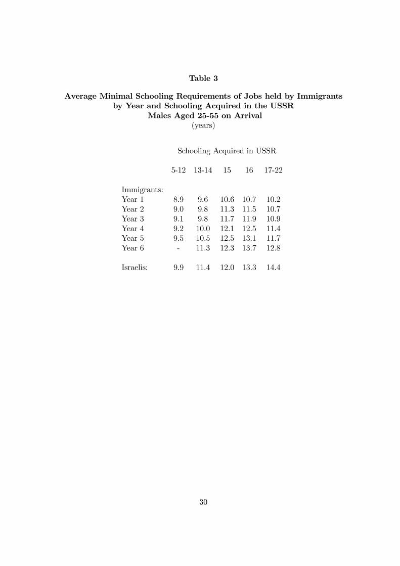
Table 3

Average Minimal Schooling Requirements of Jobs held by Immigrantsby Year and Schooling Acquired in the USSR

Males Aged 25-55 on Arrival(years)

Schooling Acquired in USSR

5-12 13-14 15 16 17-22

Immigrants:Year 1 8.9 9.6 10.6 10.7 10.2Year 2 9.0 9.8 11.3 11.5 10.7Year 3 9.1 9.8 11.7 11.9 10.9Year 4 9.2 10.0 12.1 12.5 11.4Year 5 9.5 10.5 12.5 13.1 11.7Year 6 - 11.3 12.3 13.7 12.8

Israelis: 9.9 11.4 12.0 13.3 14.4

30

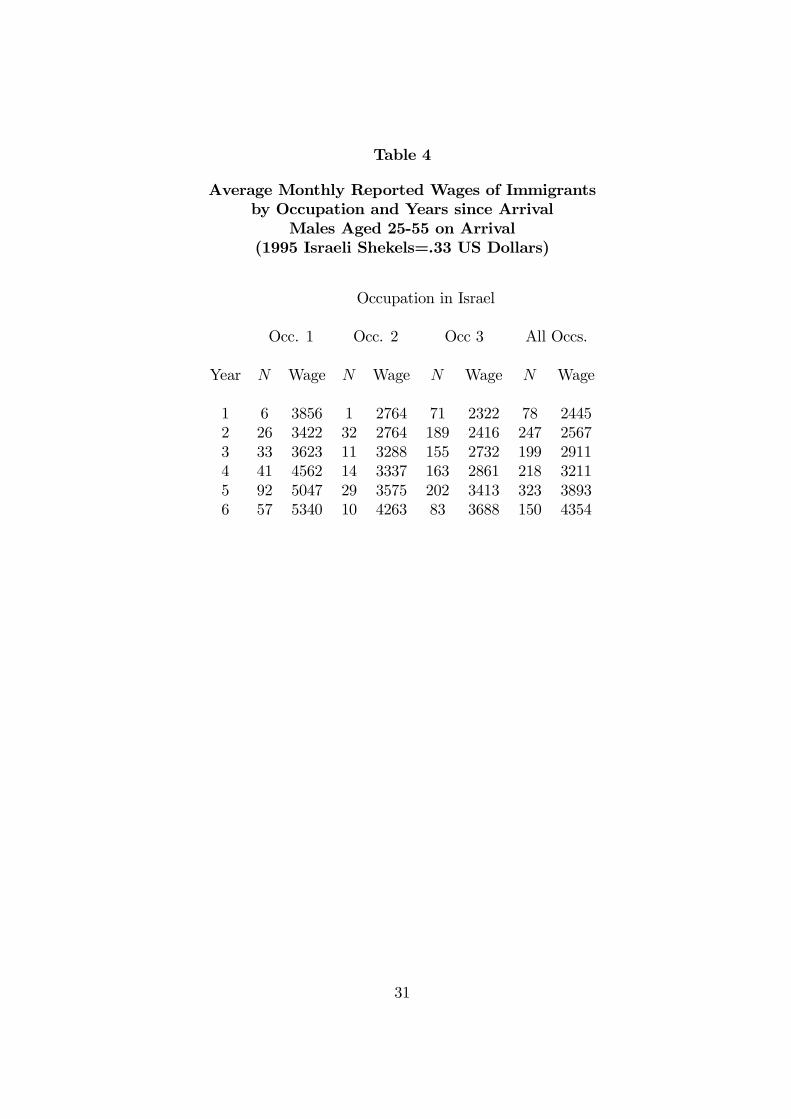
Table 4

Average Monthly Reported Wages of Immigrantsby Occupation and Years since Arrival

Males Aged 25-55 on Arrival(1995 Israeli Shekels=.33 US Dollars)

Occupation in Israel

Occ. 1 Occ. 2 Occ 3 All Occs.

Year N Wage N Wage N Wage N Wage

1 6 3856 1 2764 71 2322 78 24452 26 3422 32 2764 189 2416 247 25673 33 3623 11 3288 155 2732 199 29114 41 4562 14 3337 163 2861 218 32115 92 5047 29 3575 202 3413 323 38936 57 5340 10 4263 83 3688 150 4354

31

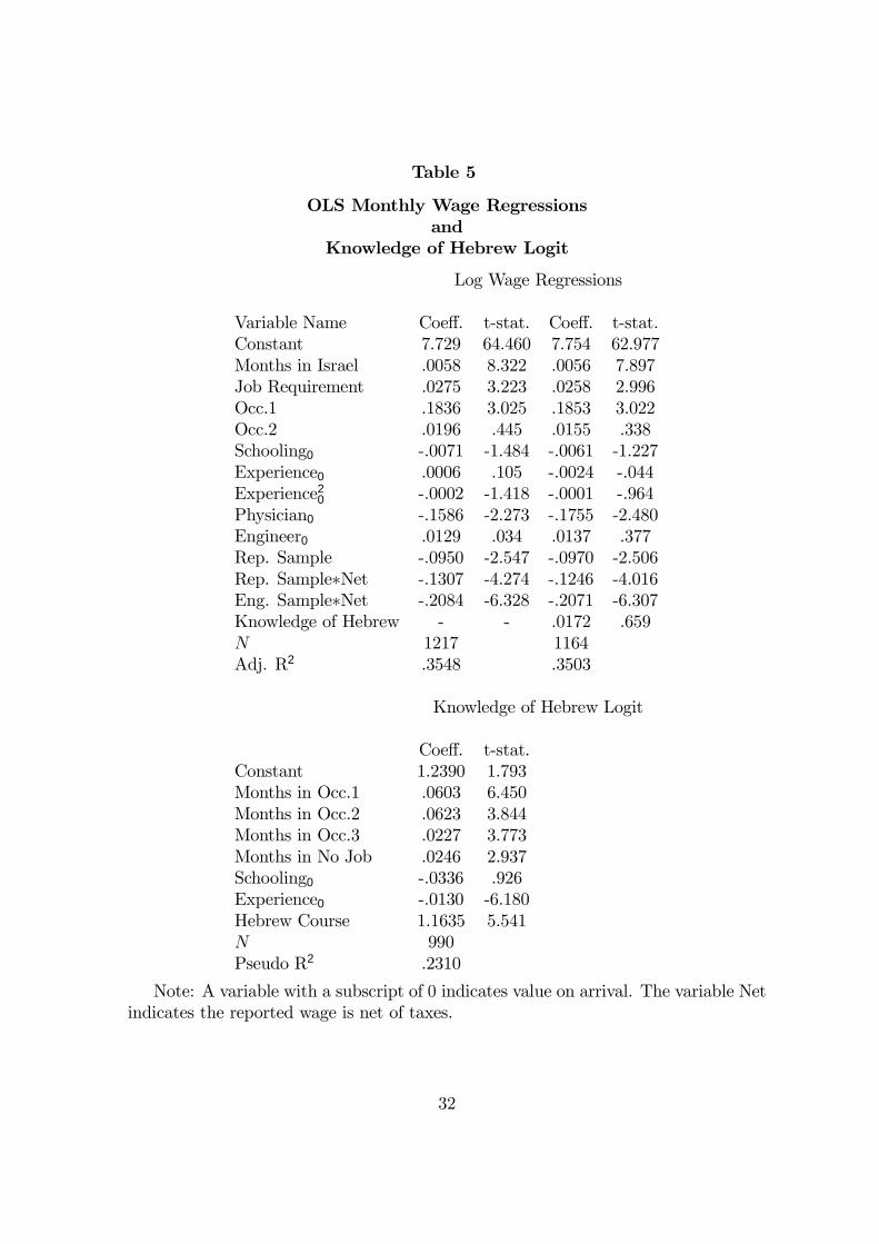
Table 5

OLS Monthly Wage Regressionsand

Knowledge of Hebrew Logit

Log Wage Regressions

Variable Name Coeff. t-stat. Coeff. t-stat.Constant 7.729 64.460 7.754 62.977Months in Israel .0058 8.322 .0056 7.897Job Requirement .0275 3.223 .0258 2.996Occ.1 .1836 3.025 .1853 3.022Occ.2 .0196 .445 .0155 .338Schooling0 -.0071 -1.484 -.0061 -1.227Experience0 .0006 .105 -.0024 -.044Experience2

0 -.0002 -1.418 -.0001 -.964Physician0 -.1586 -2.273 -.1755 -2.480Engineer0 .0129 .034 .0137 .377Rep. Sample -.0950 -2.547 -.0970 -2.506Rep. Sample∗Net -.1307 -4.274 -.1246 -4.016Eng. Sample∗Net -.2084 -6.328 -.2071 -6.307Knowledge of Hebrew - - .0172 .659N 1217 1164Adj. R2 .3548 .3503

Knowledge of Hebrew Logit

Coeff. t-stat.Constant 1.2390 1.793Months in Occ.1 .0603 6.450Months in Occ.2 .0623 3.844Months in Occ.3 .0227 3.773Months in No Job .0246 2.937Schooling0 -.0336 .926Experience0 -.0130 -6.180Hebrew Course 1.1635 5.541N 990Pseudo R2 .2310

Note: A variable with a subscript of 0 indicates value on arrival. The variable Netindicates the reported wage is net of taxes.

32

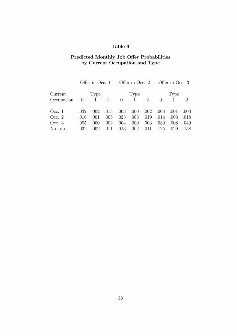
Table 6

Predicted Monthly Job Offer Probabilitiesby Current Occupation and Type

Offer in Occ. 1 Offer in Occ. 2 Offer in Occ. 3

Current Type Type TypeOccupation 0 1 2 0 1 2 0 1 2

Occ. 1 .032 .002 .013 .003 .000 .002 .003 .001 .003Occ. 2 .016 .001 .005 .023 .003 .019 .014 .003 .018Occ. 3 .005 .000 .002 .004 .000 .003 .039 .008 .049No Job .032 .002 .011 .013 .002 .011 .125 .029 .158

33

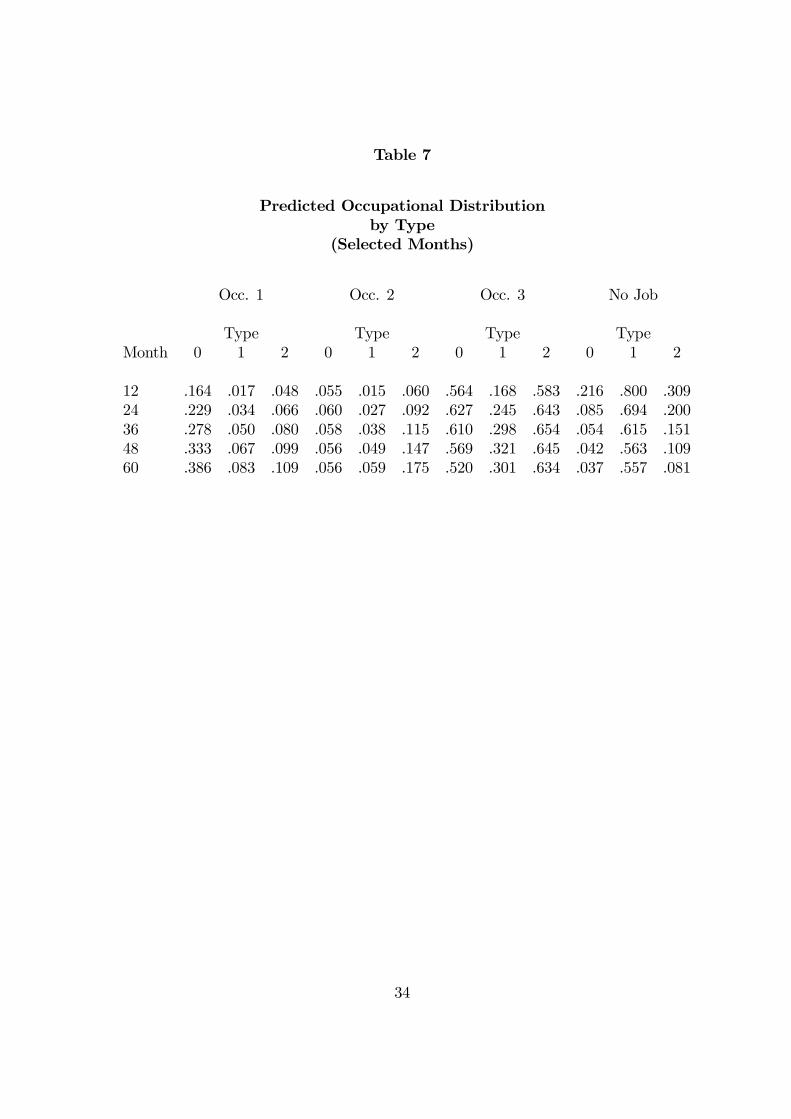
Table 7

Predicted Occupational Distributionby Type

(Selected Months)

Occ. 1 Occ. 2 Occ. 3 No Job

Type Type Type TypeMonth 0 1 2 0 1 2 0 1 2 0 1 2

12 .164 .017 .048 .055 .015 .060 .564 .168 .583 .216 .800 .30924 .229 .034 .066 .060 .027 .092 .627 .245 .643 .085 .694 .20036 .278 .050 .080 .058 .038 .115 .610 .298 .654 .054 .615 .15148 .333 .067 .099 .056 .049 .147 .569 .321 .645 .042 .563 .10960 .386 .083 .109 .056 .059 .175 .520 .301 .634 .037 .557 .081

34

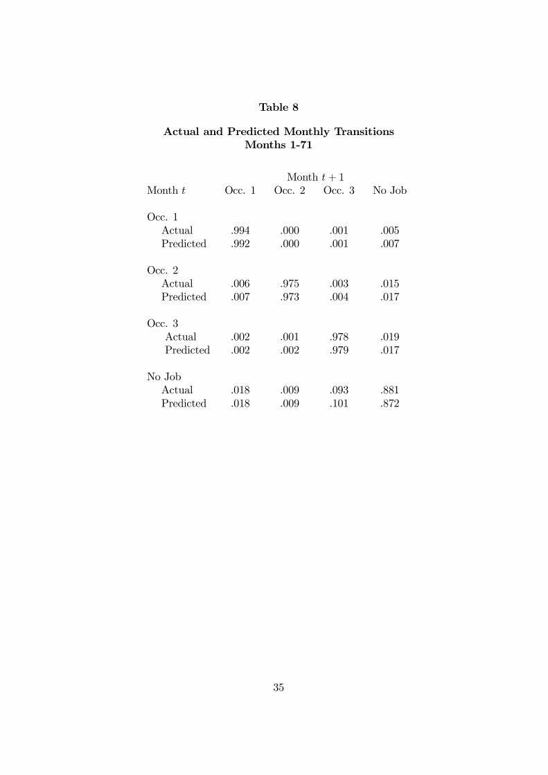
Table 8

Actual and Predicted Monthly TransitionsMonths 1-71

Month t+ 1Month t Occ. 1 Occ. 2 Occ. 3 No Job

Occ. 1Actual .994 .000 .001 .005Predicted .992 .000 .001 .007

Occ. 2Actual .006 .975 .003 .015Predicted .007 .973 .004 .017

Occ. 3Actual .002 .001 .978 .019Predicted .002 .002 .979 .017

No JobActual .018 .009 .093 .881Predicted .018 .009 .101 .872

35

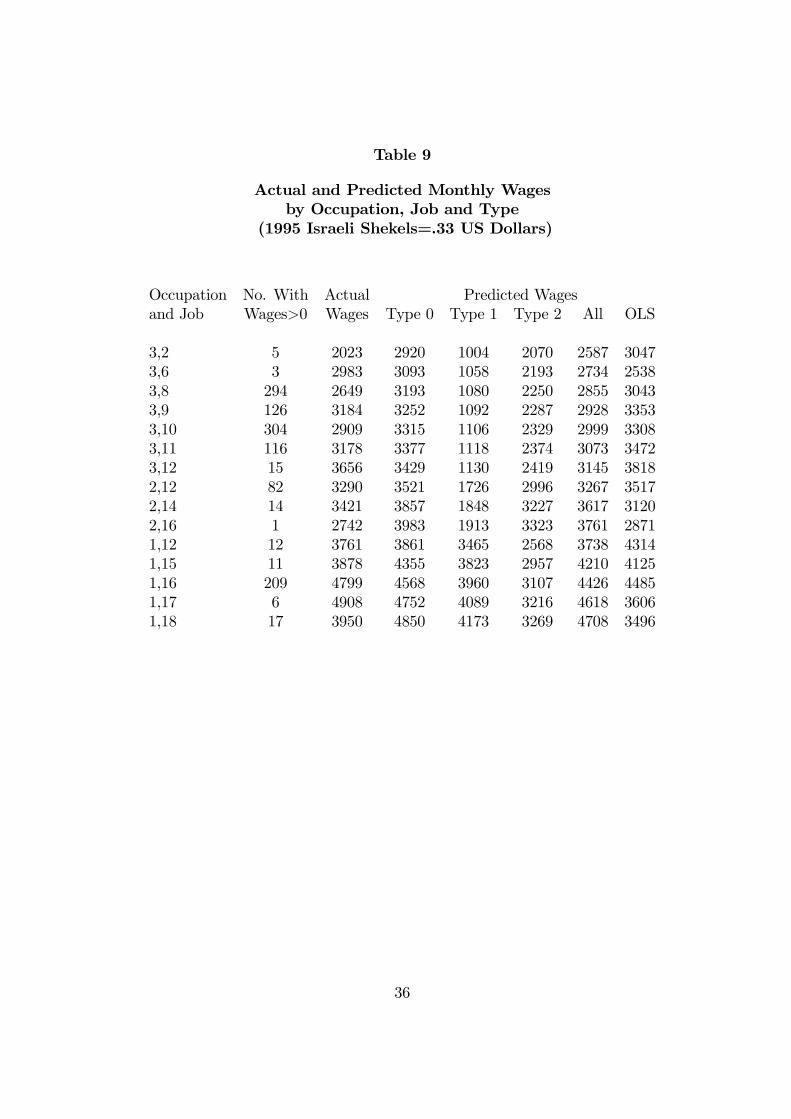
Table 9

Actual and Predicted Monthly Wagesby Occupation, Job and Type

(1995 Israeli Shekels=.33 US Dollars)

Occupation No. With Actual Predicted Wagesand Job Wages>0 Wages Type 0 Type 1 Type 2 All OLS

3,2 5 2023 2920 1004 2070 2587 30473,6 3 2983 3093 1058 2193 2734 25383,8 294 2649 3193 1080 2250 2855 30433,9 126 3184 3252 1092 2287 2928 33533,10 304 2909 3315 1106 2329 2999 33083,11 116 3178 3377 1118 2374 3073 34723,12 15 3656 3429 1130 2419 3145 38182,12 82 3290 3521 1726 2996 3267 35172,14 14 3421 3857 1848 3227 3617 31202,16 1 2742 3983 1913 3323 3761 28711,12 12 3761 3861 3465 2568 3738 43141,15 11 3878 4355 3823 2957 4210 41251,16 209 4799 4568 3960 3107 4426 44851,17 6 4908 4752 4089 3216 4618 36061,18 17 3950 4850 4173 3269 4708 3496

36

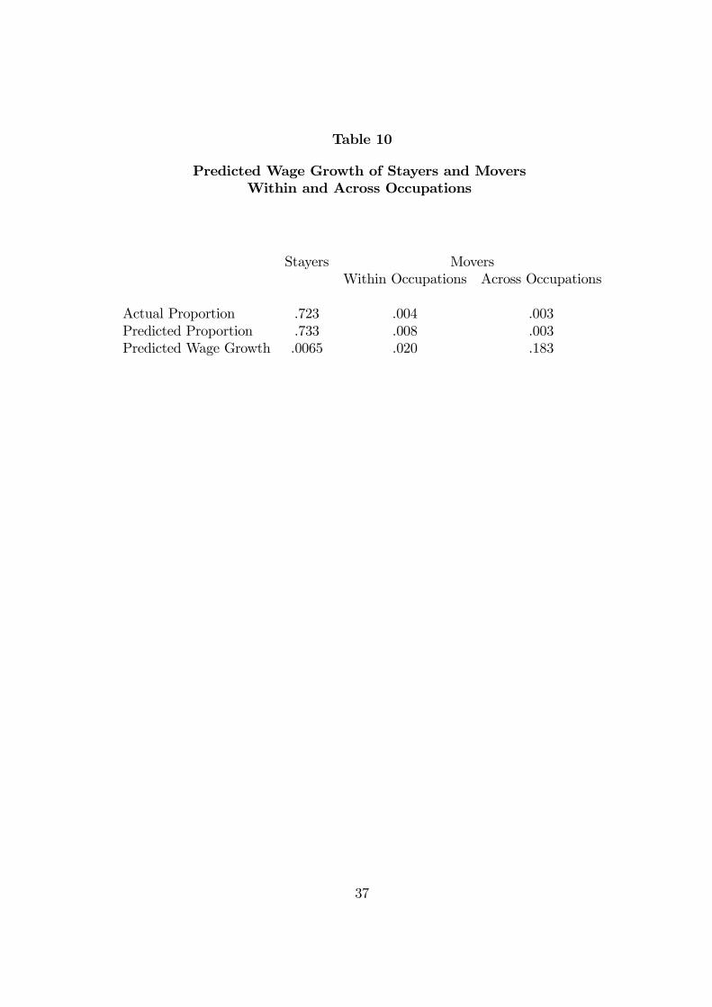
Table 10

Predicted Wage Growth of Stayers and MoversWithin and Across Occupations

Stayers MoversWithin Occupations Across Occupations

Actual Proportion .723 .004 .003Predicted Proportion .733 .008 .003Predicted Wage Growth .0065 .020 .183

37

Table 11

Occupational Choice DistributionImmigrants from Occupation 1 in USSR

by Age at Arrival

Younger than 40 Older than 40Occ. 1 Occ. 2 Occ. 3 No Job Occ. 1 Occ. 2 Occ. 3 No Job

Year1 .175 .069 .483 .273 .123 .039 .560 .2772 .246 .087 .522 .145 .159 .043 .647 .1503 .289 .092 .514 .105 .177 .042 .668 .1134 .320 .090 .506 .084 .187 .040 .678 .0945 .342 .086 .498 .073 .195 .038 .682 .0856 .347 .085 .495 .073 .197 .038 .680 .0857 .397 .087 .435 .081 .239 .048 .635 .0788 .418 .088 .417 .076 .261 .052 .619 .0699 .437 .089 .400 .073 .280 .055 .601 .06410 .455 .088 .385 .071 .305 .058 .577 .06111 .472 .087 .371 .07012 .487 .086 .359 .06813 .501 .084 .349 .06614 .514 .082 .339 .06415 .526 .081 .331 .06316 .536 .079 .324 .06117 .546 .077 .317 .06018 .554 .076 .311 .05819 .563 .074 .306 .05720 .570 .073 .302 .05621 .576 .071 .298 .05522 .582 .070 .295 .05323 .588 .068 .291 .05324 .593 .067 .289 .05225 .596 .066 .287 .051

38

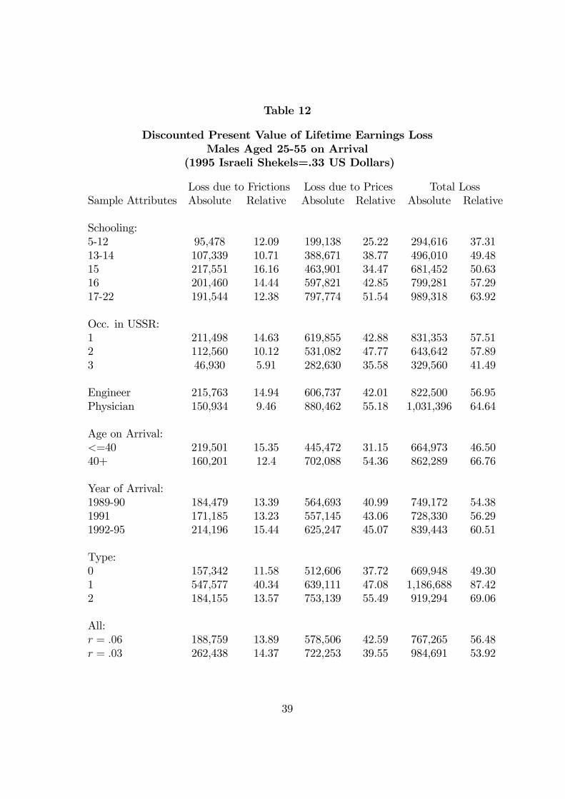
Table 12

Discounted Present Value of Lifetime Earnings LossMales Aged 25-55 on Arrival

(1995 Israeli Shekels=.33 US Dollars)

Loss due to Frictions Loss due to Prices Total LossSample Attributes Absolute Relative Absolute Relative Absolute Relative

Schooling:5-12 95,478 12.09 199,138 25.22 294,616 37.3113-14 107,339 10.71 388,671 38.77 496,010 49.4815 217,551 16.16 463,901 34.47 681,452 50.6316 201,460 14.44 597,821 42.85 799,281 57.2917-22 191,544 12.38 797,774 51.54 989,318 63.92

Occ. in USSR:1 211,498 14.63 619,855 42.88 831,353 57.512 112,560 10.12 531,082 47.77 643,642 57.893 46,930 5.91 282,630 35.58 329,560 41.49

Engineer 215,763 14.94 606,737 42.01 822,500 56.95Physician 150,934 9.46 880,462 55.18 1,031,396 64.64

Age on Arrival:<=40 219,501 15.35 445,472 31.15 664,973 46.5040+ 160,201 12.4 702,088 54.36 862,289 66.76

Year of Arrival:1989-90 184,479 13.39 564,693 40.99 749,172 54.381991 171,185 13.23 557,145 43.06 728,330 56.291992-95 214,196 15.44 625,247 45.07 839,443 60.51

Type:0 157,342 11.58 512,606 37.72 669,948 49.301 547,577 40.34 639,111 47.08 1,186,688 87.422 184,155 13.57 753,139 55.49 919,294 69.06

All:r = .06 188,759 13.89 578,506 42.59 767,265 56.48r = .03 262,438 14.37 722,253 39.55 984,691 53.92

39

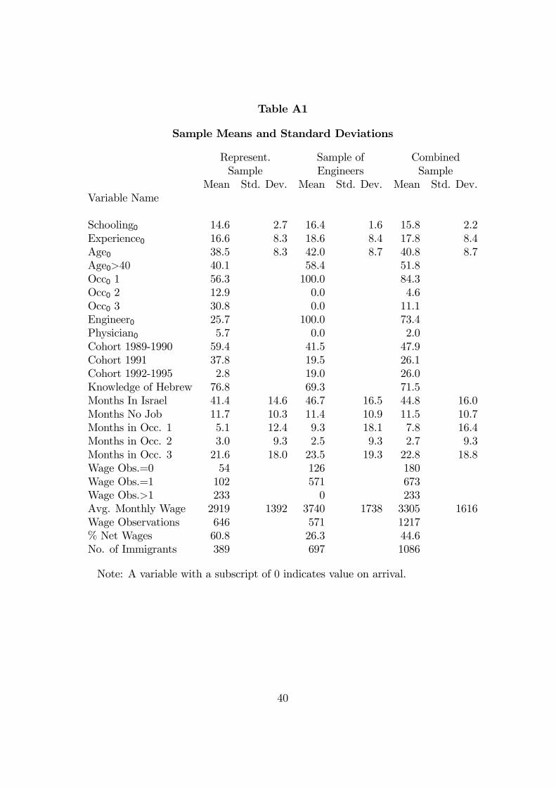
Table A1

Sample Means and Standard Deviations

Represent. Sample of CombinedSample Engineers Sample

Mean Std. Dev. Mean Std. Dev. Mean Std. Dev.Variable Name

Schooling0 14.6 2.7 16.4 1.6 15.8 2.2Experience0 16.6 8.3 18.6 8.4 17.8 8.4Age0 38.5 8.3 42.0 8.7 40.8 8.7Age0>40 40.1 58.4 51.8Occ0 1 56.3 100.0 84.3Occ0 2 12.9 0.0 4.6Occ0 3 30.8 0.0 11.1Engineer0 25.7 100.0 73.4Physician0 5.7 0.0 2.0Cohort 1989-1990 59.4 41.5 47.9Cohort 1991 37.8 19.5 26.1Cohort 1992-1995 2.8 19.0 26.0Knowledge of Hebrew 76.8 69.3 71.5Months In Israel 41.4 14.6 46.7 16.5 44.8 16.0Months No Job 11.7 10.3 11.4 10.9 11.5 10.7Months in Occ. 1 5.1 12.4 9.3 18.1 7.8 16.4Months in Occ. 2 3.0 9.3 2.5 9.3 2.7 9.3Months in Occ. 3 21.6 18.0 23.5 19.3 22.8 18.8Wage Obs.=0 54 126 180Wage Obs.=1 102 571 673Wage Obs.>1 233 0 233Avg. Monthly Wage 2919 1392 3740 1738 3305 1616Wage Observations 646 571 1217% Net Wages 60.8 26.3 44.6No. of Immigrants 389 697 1086

Note: A variable with a subscript of 0 indicates value on arrival.

40

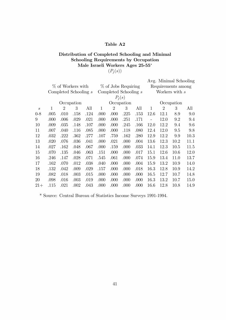
Table A2

Distribution of Completed Schooling and MinimalSchooling Requirements by OccupationMale Israeli Workers Ages 25-55∗

(Pj(s))

Avg. Minimal Schooling% of Workers with % of Jobs Requiring Requirements among

Completed Schooling s Completed Schooling s Workers with sPj(s)

Occupation Occupation Occupations 1 2 3 All 1 2 3 All 1 2 3 All0-8 .005 .010 .158 .124 .000 .000 .225 .153 12.6 12.1 8.9 9.09 .000 .006 .029 .021 .000 .000 .251 .171 - 12.0 9.2 9.410 .009 .035 .148 .107 .000 .000 .245 .166 12.0 12.2 9.4 9.611 .007 .040 .116 .085 .000 .000 .118 .080 12.4 12.0 9.5 9.812 .032 .222 .362 .277 .107 .759 .162 .280 12.9 12.2 9.9 10.313 .020 .076 .036 .041 .000 .021 .000 .004 13.6 12.3 10.2 11.114 .027 .162 .048 .067 .000 .159 .000 .033 14.1 12.3 10.5 11.515 .070 .135 .046 .063 .151 .000 .000 .017 15.1 12.6 10.6 12.016 .246 .147 .028 .071 .545 .061 .000 .074 15.9 13.4 11.0 13.717 .162 .070 .012 .038 .040 .000 .000 .004 15.9 13.2 10.9 14.018 .132 .042 .009 .029 .157 .000 .000 .018 16.3 12.8 10.9 14.219 .082 .018 .003 .015 .000 .000 .000 .000 16.5 12.7 10.7 14.820 .098 .016 .003 .019 .000 .000 .000 .000 16.3 13.2 10.7 15.021+ .115 .021 .002 .043 .000 .000 .000 .000 16.6 12.8 10.8 14.9

* Source: Central Bureau of Statistics Income Surveys 1991-1994.

41

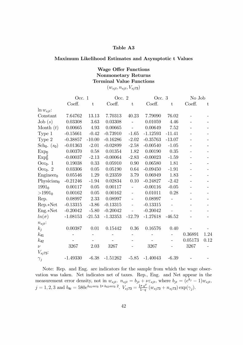
Table A3

Maximum Likelihood Estimates and Asymptotic t Values

Wage Offer FunctionsNonmonetary Returns

Terminal Value Functions(wsjt, nsjt, Vsj73)

Occ. 1 Occ. 2 Occ. 3 No JobCoeff. t Coeff. t Coeff. t Coeff. t

lnwsjt:Constant 7.64762 13.13 7.70313 40.23 7.79090 76.02 - -Job (s) 0.03308 3.63 0.03308 - 0.01059 4.46 - -Month (t) 0.00665 4.93 0.00665 - 0.00649 7.52 - -Type 1 -0.15661 -0.42 -0.73910 -1.65 -1.12593 -11.41 - -Type 2 -0.38857 -10.00 -0.16286 -2.02 -0.35763 -13.07 - -Sch0. (s0) -0.01363 -2.01 -0.02899 -2.58 -0.00540 -1.05 - -Exp0 0.00370 0.58 0.01354 1.82 0.00190 0.35 - -Exp2

0 -0.00037 -2.13 -0.00064 -2.83 -0.00023 -1.59 - -Occ0. 1 0.19038 0.33 0.05910 0.90 0.06580 1.81 - -Occ0. 2 0.03306 0.05 0.05190 0.64 -0.09450 -1.91 - -Engineer0 0.05546 1.29 0.23359 3.79 0.06949 1.83 - -Physician0 -0.21246 -1.94 0.02834 0.10 -0.24827 -2.42 - -19910 0.00117 0.05 0.00117 - -0.00116 -0.05 - ->19910 0.00162 0.05 0.00162 - 0.01011 0.28 - -Rep. 0.08997 2.33 0.08997 - 0.08997 - - -Rep.∗Net -0.13315 -3.86 -0.13315 - -0.13315 - - -Eng.∗Net -0.20042 -5.80 -0.20042 - -0.20042 - - -ln(σ) -1.08153 -21.53 -1.32353 -12.79 -1.27618 -46.52 - -nsjt:kj 0.00387 0.01 0.15442 0.36 0.16576 0.40 - -k41 - - - - - - 0.36891 1.24k42 - - - - - - 0.05173 0.12ν 3267 2.03 3267 - 3267 - 3267 -Vsj73:γj -1.49330 -6.38 -1.51262 -5.85 -1.40043 -6.39 - -

Note: Rep. and Eng. are indicators for the sample from which the wage obser-vation was taken. Net indicates net of taxes. Rep., Eng. and Net appear in themeasurement error density, not in wsjt. nsjt = bjt + νεsjt, where bjt = (ekj − 1)wsjt,j = 1, 2, 3 and b4t = 580ek41occ0 1+k42occ0 2. Vsj73 =

1+qT

1−q (wsj73 + nsj73) exp(γj).

42

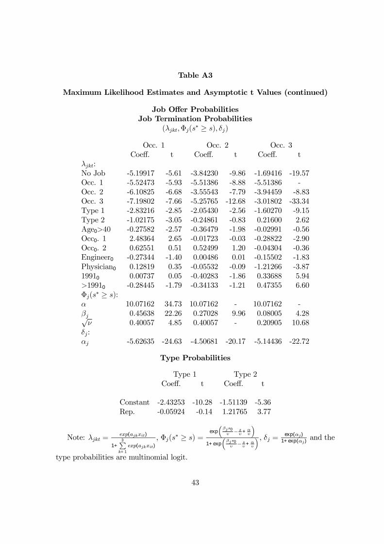
Table A3

Maximum Likelihood Estimates and Asymptotic t Values (continued)

Job Offer ProbabilitiesJob Termination Probabilities

(λjkt,Φj(s∗ ≥ s), δj)

Occ. 1 Occ. 2 Occ. 3Coeff. t Coeff. t Coeff. t

λjkt:No Job -5.19917 -5.61 -3.84230 -9.86 -1.69416 -19.57Occ. 1 -5.52473 -5.93 -5.51386 -8.88 -5.51386 -Occ. 2 -6.10825 -6.68 -3.55543 -7.79 -3.94459 -8.83Occ. 3 -7.19802 -7.66 -5.25765 -12.68 -3.01802 -33.34Type 1 -2.83216 -2.85 -2.05430 -2.56 -1.60270 -9.15Type 2 -1.02175 -3.05 -0.24861 -0.83 0.21600 2.62Age0>40 -0.27582 -2.57 -0.36479 -1.98 -0.02991 -0.56Occ0. 1 2.48364 2.65 -0.01723 -0.03 -0.28822 -2.90Occ0. 2 0.62551 0.51 0.52499 1.20 -0.04304 -0.36Engineer0 -0.27344 -1.40 0.00486 0.01 -0.15502 -1.83Physician0 0.12819 0.35 -0.05532 -0.09 -1.21266 -3.8719910 0.00737 0.05 -0.40283 -1.86 0.33688 5.94>19910 -0.28445 -1.79 -0.34133 -1.21 0.47355 6.60Φj(s

∗ ≥ s):α 10.07162 34.73 10.07162 - 10.07162 -βj 0.45638 22.26 0.27028 9.96 0.08005 4.28√ν 0.40057 4.85 0.40057 - 0.20905 10.68

δj:αj -5.62635 -24.63 -4.50681 -20.17 -5.14436 -22.72

Type Probabilities

Type 1 Type 2Coeff. t Coeff. t

Constant -2.43253 -10.28 -1.51139 -5.36Rep. -0.05924 -0.14 1.21765 3.77

Note: λjkt =exp(ajkxit)

1+3P

k=1

exp(ajkxit)

, Φj(s∗ ≥ s) =exp

³βjs0υ− sυ

+αυ

´1+exp

³βjs0υ− sυ

+αυ

´ , δj = exp(αj)

1+exp(αj)and the

type probabilities are multinomial logit.

43

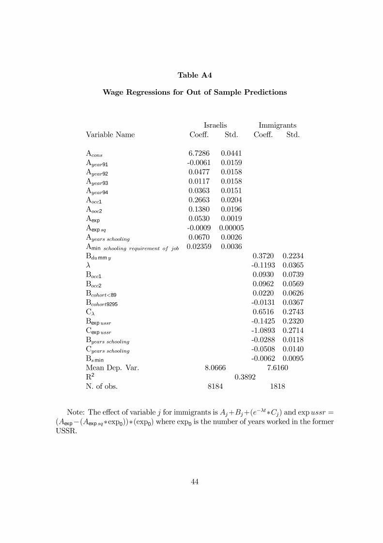
Table A4

Wage Regressions for Out of Sample Predictions

Israelis ImmigrantsVariable Name Coeff. Std. Coeff. Std.

Acons 6.7286 0.0441Ayear91 -0.0061 0.0159Ayear92 0.0477 0.0158Ayear93 0.0117 0.0158Ayear94 0.0363 0.0151Aocc1 0.2663 0.0204Aooc2 0.1380 0.0196Aexp 0.0530 0.0019Aexp sq -0.0009 0.00005Ayears schooling 0.0670 0.0026Amin schooling requirement of job 0.02359 0.0036Bdumm y 0.3720 0.2234λ -0.1193 0.0365Bocc1 0.0930 0.0739Bocc2 0.0962 0.0569Bcohort<89 0.0220 0.0626Bcohort9295 -0.0131 0.0367Cλ 0.6516 0.2743Bexpussr -0.1425 0.2320Cexpussr -1.0893 0.2714Byears schooling -0.0288 0.0118Cyears schooling -0.0508 0.0140Bsmin -0.0062 0.0095Mean Dep. Var. 8.0666 7.6160R2 0.3892N. of obs. 8184 1818

Note: The effect of variable j for immigrants is Aj+Bj+(e−λt∗Cj) and expussr =(Aexp−(Aexp sq∗exp0))∗(exp0) where exp0 is the number of years worked in the formerUSSR.

44

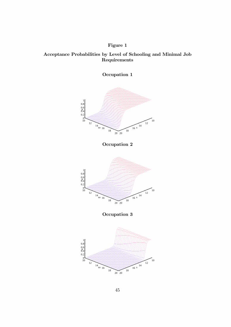
Figure 1

Acceptance Probabilities by Level of Schooling and Minimal JobRequirements

Occupation 1

1012

1416

1820

s

1012

1416

1820

so

00.20.40.60.8

1

p

Occupation 2

1012

1416

1820

s

1012

1416

1820

so

00.20.40.60.8

1

p

Occupation 3

1012

1416

1820

s

1012

1416

1820

so

00.20.40.60.8

1

p

45

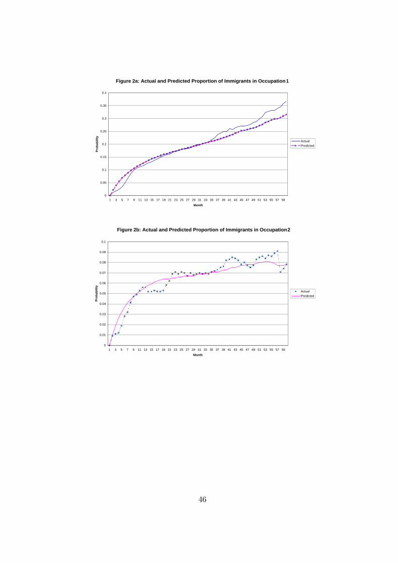
Figure 2a: Actual and Predicted Proportion of Immigrants in Occupation 1

0

0.05

0.1

0.15

0.2

0.25

0.3

0.35

0.4

1 3 5 7 9 11 13 15 17 19 21 23 25 27 29 31 33 35 37 39 41 43 45 47 49 51 53 55 57 59Month

Prob

abili

ty

ActualPredicted

�������������

������

���������

��������

������

����������

���������������������������������

���������

��������

������������������������������������������������������

��������������

���������������������������

�������������

�����������������������

�������������������������

���������

Figure 2b: Actual and Predicted Proportion of Immigrants in Occupation 2

0

0.01

0.02

0.03

0.04

0.05

0.06

0.07

0.08

0.09

0.1

1 3 5 7 9 11 13 15 17 19 21 23 25 27 29 31 33 35 37 39 41 43 45 47 49 51 53 55 57 59Month

Prob

abili

ty

��������ActualPredicted

46

����������������

������

������������

��������

������

��������

��������

�������������������

����������������������������������������������������������������������������������������������������������������������

��������������

���������������������������������������������

���������������������

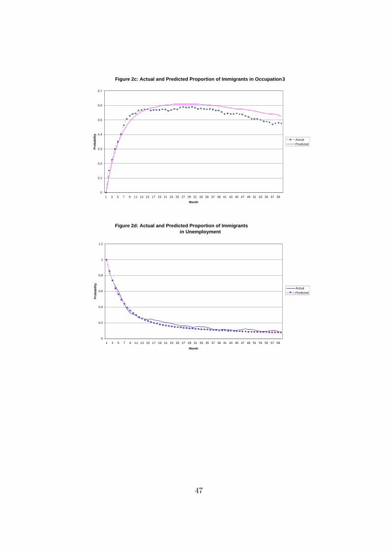
Figure 2c: Actual and Predicted Proportion of Immigrants in Occupation 3

0

0.1

0.2

0.3

0.4

0.5

0.6

0.7

1 3 5 7 9 11 13 15 17 19 21 23 25 27 29 31 33 35 37 39 41 43 45 47 49 51 53 55 57 59Month

Prob

abili

ty ��������ActualPredicted

��������������������

������������

��������������������������������

������������������������

��������������������������������������������

����������������������������������������������������������������������������������������������������������������������������������������������������������������

Figure 2d: Actual and Predicted Proportion of Immigrants in Unemployment

0

0.2

0.4

0.6

0.8

1

1.2

1 3 5 7 9 11 13 15 17 19 21 23 25 27 29 31 33 35 37 39 41 43 45 47 49 51 53 55 57 59

Month

Prob

abili

ty

Actual��������Predicted

47

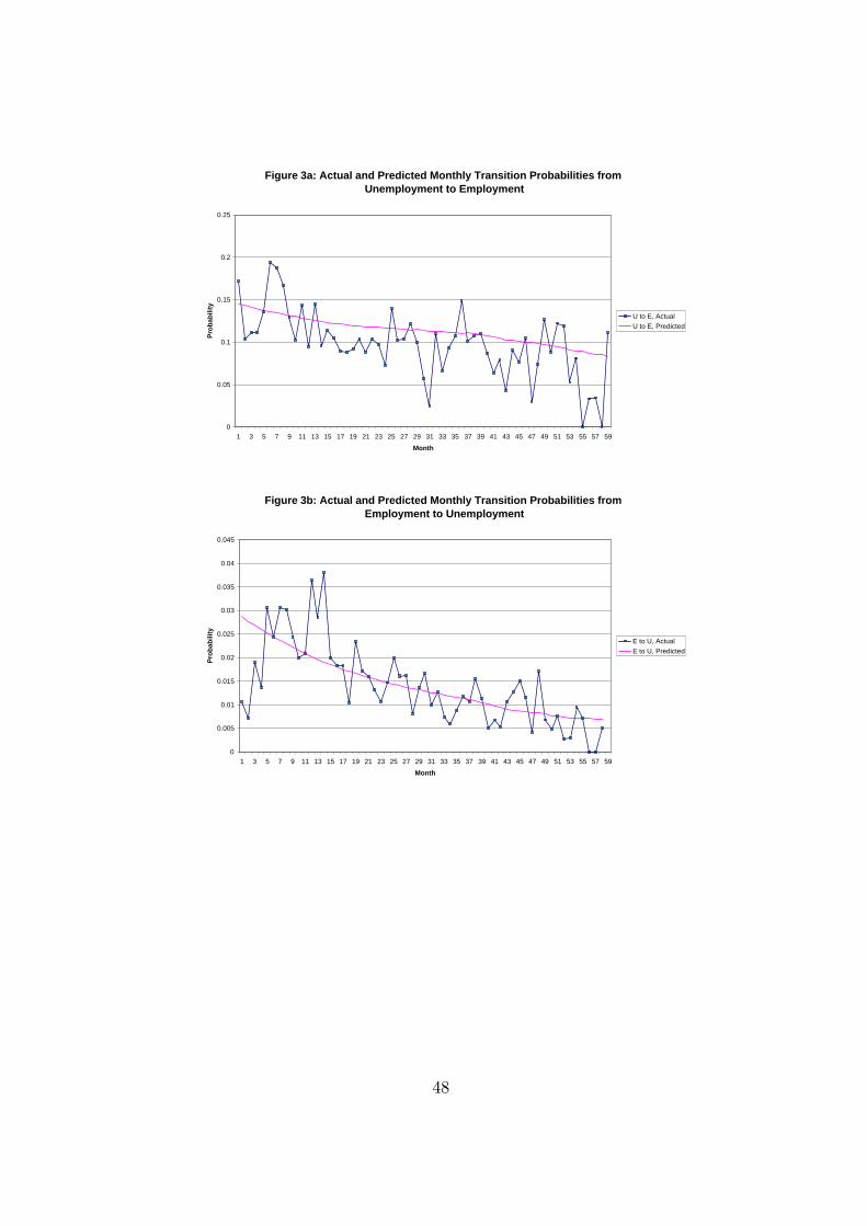
Figure 3a: Actual and Predicted Monthly Transition Probabilities from Unemployment to Employment

0

0.05

0.1

0.15

0.2

0.25

1 3 5 7 9 11 13 15 17 19 21 23 25 27 29 31 33 35 37 39 41 43 45 47 49 51 53 55 57 59Month

Prob

abili

ty

U to E, ActualU to E, Predicted

Figure 3b: Actual and Predicted Monthly Transition Probabilities from Employment to Unemployment

0

0.005

0.01

0.015

0.02

0.025

0.03

0.035

0.04

0.045

1 3 5 7 9 11 13 15 17 19 21 23 25 27 29 31 33 35 37 39 41 43 45 47 49 51 53 55 57 59Month

Prob

abili

ty

E to U, ActualE to U, Predicted

48

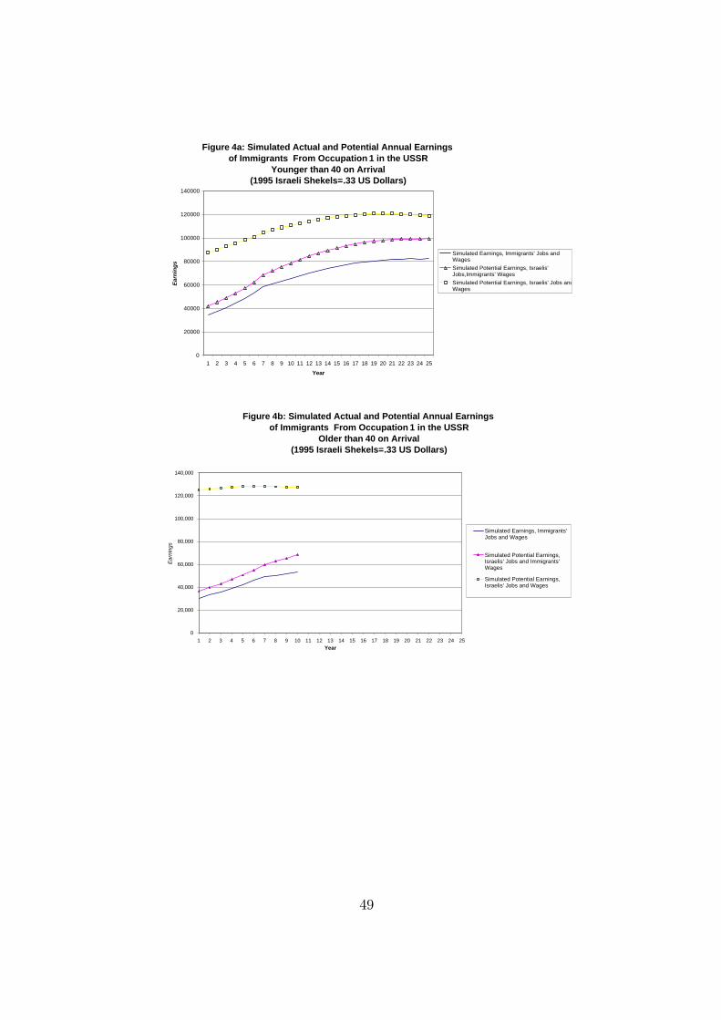
Figure 4a: Simulated Actual and Potential Annual Earnings of Immigrants From Occupation 1 in the USSR

Younger than 40 on Arrival(1995 Israeli Shekels=.33 US Dollars)

0

20000

40000

60000

80000

100000

120000

140000

1 2 3 4 5 6 7 8 9 10 11 12 13 14 15 16 17 18 19 20 21 22 23 24 25Year

Earn

ings

Simulated Earnings, Immigrants' Jobs andWagesSimulated Potential Earnings, Israelis'Jobs,Immigrants' WagesSimulated Potential Earnings, Israelis' Jobs andWages

Figure 4b: Simulated Actual and Potential Annual Earnings of Immigrants From Occupation 1 in the USSR

Older than 40 on Arrival(1995 Israeli Shekels=.33 US Dollars)

0

20,000

40,000

60,000

80,000

100,000

120,000

140,000

1 2 3 4 5 6 7 8 9 10 11 12 13 14 15 16 17 18 19 20 21 22 23 24 25Year

Earn

ings

Simulated Earnings, Immigrants'Jobs and Wages

Simulated Potential Earnings,Israelis' Jobs and Immigrants'Wages

Simulated Potential Earnings,Israelis' Jobs and Wages

49