Embed Size (px)
Citation preview
������������ ��
���������������������������������
Controller software IRC5RobotWare 5.12


© C
opyr
ight
200
4-20
09 A
BB
. All
righ
ts r
eser
ved.
Application manual
Additional axes and stand alone controllerRobotWare-OS 5.0
Document ID: 3HAC021395-001
Revision: H
© C
opyr
ight
200
4-20
09 A
BB
. All
righ
ts r
eser
ved.
The information in this manual is subject to change without notice and should not be construed as a commitment by ABB. ABB assumes no responsibility for any errors that may appear in this manual.
Except as may be expressly stated anywhere in this manual, nothing herein shall be construed as any kind of guarantee or warranty by ABB for losses, damages to persons or property, fitness for a specific purpose or the like.
In no event shall ABB be liable for incidental or consequential damages arising from use of this manual and products described herein.
This manual and parts thereof must not be reproduced or copied without ABB's written permission, and contents thereof must not be imparted to a third party nor be used for any unauthorized purpose. Contravention will be prosecuted.
Additional copies of this manual may be obtained from ABB at its then current charge.
© Copyright 2004-2009 ABB All rights reserved.
ABB ABRobotics Products
SE-721 68 Västerås Sweden
Table of Contents
33HAC021395-001 Revision: H
© C
opyr
ight
200
4-20
09 A
BB
. All
righ
ts r
eser
ved.
Manual overview . . . . . . . . . . . . . . . . . . . . . . . . . . . . . . . . . . . . . . . . . . . . . . . . . . . . . . . . . . . . . . . . . . . . . . . 7Product documentation, M2004 . . . . . . . . . . . . . . . . . . . . . . . . . . . . . . . . . . . . . . . . . . . . . . . . . . . . . . . . . . . . 9Safety . . . . . . . . . . . . . . . . . . . . . . . . . . . . . . . . . . . . . . . . . . . . . . . . . . . . . . . . . . . . . . . . . . . . . . . . . . . . . . . 11
1 Introduction 13
1.1 Overview . . . . . . . . . . . . . . . . . . . . . . . . . . . . . . . . . . . . . . . . . . . . . . . . . . . . . . . . . . . . . . . . . . . . . . . . . 131.2 Definitions . . . . . . . . . . . . . . . . . . . . . . . . . . . . . . . . . . . . . . . . . . . . . . . . . . . . . . . . . . . . . . . . . . . . . . . . 141.3 General guidelines and limitations . . . . . . . . . . . . . . . . . . . . . . . . . . . . . . . . . . . . . . . . . . . . . . . . . . . . . . 15
2 Getting started 17
2.1 Get started with additional axes, servo guns and non-ABB robots . . . . . . . . . . . . . . . . . . . . . . . . . . . . . 17
3 Installation 19
3.1 Additional axes and servo guns . . . . . . . . . . . . . . . . . . . . . . . . . . . . . . . . . . . . . . . . . . . . . . . . . . . . . . 193.1.1 Standard additional axis (Option selected). . . . . . . . . . . . . . . . . . . . . . . . . . . . . . . . . . . . . . . . . . . 193.1.2 Template files . . . . . . . . . . . . . . . . . . . . . . . . . . . . . . . . . . . . . . . . . . . . . . . . . . . . . . . . . . . . . . . . . 223.1.3 Serial measurement system configuration . . . . . . . . . . . . . . . . . . . . . . . . . . . . . . . . . . . . . . . . . . . 24
3.2 Non ABB robots . . . . . . . . . . . . . . . . . . . . . . . . . . . . . . . . . . . . . . . . . . . . . . . . . . . . . . . . . . . . . . . . . . . 253.2.1 Introduction . . . . . . . . . . . . . . . . . . . . . . . . . . . . . . . . . . . . . . . . . . . . . . . . . . . . . . . . . . . . . . . . . . 253.2.2 Drive module for non-ABB robots. . . . . . . . . . . . . . . . . . . . . . . . . . . . . . . . . . . . . . . . . . . . . . . . . 263.2.3 Kinematic models . . . . . . . . . . . . . . . . . . . . . . . . . . . . . . . . . . . . . . . . . . . . . . . . . . . . . . . . . . . . . 27
3.2.3.1 Introduction . . . . . . . . . . . . . . . . . . . . . . . . . . . . . . . . . . . . . . . . . . . . . . . . . . . . . . . . . . . 273.2.3.2 Kinematic model XYZ . . . . . . . . . . . . . . . . . . . . . . . . . . . . . . . . . . . . . . . . . . . . . . . . . . . 283.2.3.3 Kinematic model C(Z) . . . . . . . . . . . . . . . . . . . . . . . . . . . . . . . . . . . . . . . . . . . . . . . . . . . 293.2.3.4 Kinematic model B(X) . . . . . . . . . . . . . . . . . . . . . . . . . . . . . . . . . . . . . . . . . . . . . . . . . . . 303.2.3.5 Kinematic model XYZB(Y) . . . . . . . . . . . . . . . . . . . . . . . . . . . . . . . . . . . . . . . . . . . . . . . 313.2.3.6 Kinematic model XYZC(Z)B(X) . . . . . . . . . . . . . . . . . . . . . . . . . . . . . . . . . . . . . . . . . . . 323.2.3.7 Kinematic model XYZC(Z)B(Y) . . . . . . . . . . . . . . . . . . . . . . . . . . . . . . . . . . . . . . . . . . . 333.2.3.8 Kinematic model XYZB(X)A(Z) . . . . . . . . . . . . . . . . . . . . . . . . . . . . . . . . . . . . . . . . . . . 343.2.3.9 Kinematic model XYZB(Y)A(Z) . . . . . . . . . . . . . . . . . . . . . . . . . . . . . . . . . . . . . . . . . . . 353.2.3.10 Kinematic model XYZC(Z)B(X)A(Z) . . . . . . . . . . . . . . . . . . . . . . . . . . . . . . . . . . . . . . 363.2.3.11 Kinematic model XYZC(Z)B(Y)A(Z) . . . . . . . . . . . . . . . . . . . . . . . . . . . . . . . . . . . . . . 373.2.3.12 Kinematic model XYZC(Z)A(X) . . . . . . . . . . . . . . . . . . . . . . . . . . . . . . . . . . . . . . . . . . 383.2.3.13 Kinematic model XYZC(Z)A(Y) . . . . . . . . . . . . . . . . . . . . . . . . . . . . . . . . . . . . . . . . . . 393.2.3.14 Kinematic model XZ. . . . . . . . . . . . . . . . . . . . . . . . . . . . . . . . . . . . . . . . . . . . . . . . . . . . 403.2.3.15 Kinematic model XZC(Z) . . . . . . . . . . . . . . . . . . . . . . . . . . . . . . . . . . . . . . . . . . . . . . . . 413.2.3.16 Kinematic model XZB(X). . . . . . . . . . . . . . . . . . . . . . . . . . . . . . . . . . . . . . . . . . . . . . . . 423.2.3.17 Kinematic model XZB(Y). . . . . . . . . . . . . . . . . . . . . . . . . . . . . . . . . . . . . . . . . . . . . . . . 433.2.3.18 Kinematic model XZC(Z)B(X). . . . . . . . . . . . . . . . . . . . . . . . . . . . . . . . . . . . . . . . . . . . 443.2.3.19 Kinematic model XZC(Z)B(Y). . . . . . . . . . . . . . . . . . . . . . . . . . . . . . . . . . . . . . . . . . . . 453.2.3.20 Kinematic model XZB(X)A(Z). . . . . . . . . . . . . . . . . . . . . . . . . . . . . . . . . . . . . . . . . . . . 463.2.3.21 Kinematic model XZB(Y)A(Z). . . . . . . . . . . . . . . . . . . . . . . . . . . . . . . . . . . . . . . . . . . . 473.2.3.22 Kinematic model XZC(Z)B(X)A(Z) . . . . . . . . . . . . . . . . . . . . . . . . . . . . . . . . . . . . . . . . 483.2.3.23 Kinematic model YZ. . . . . . . . . . . . . . . . . . . . . . . . . . . . . . . . . . . . . . . . . . . . . . . . . . . . 493.2.3.24 Kinematic model YZC(Z) . . . . . . . . . . . . . . . . . . . . . . . . . . . . . . . . . . . . . . . . . . . . . . . . 503.2.3.25 Kinematic model YZB(X). . . . . . . . . . . . . . . . . . . . . . . . . . . . . . . . . . . . . . . . . . . . . . . . 513.2.3.26 Kinematic model YZB(Y). . . . . . . . . . . . . . . . . . . . . . . . . . . . . . . . . . . . . . . . . . . . . . . . 523.2.3.27 Kinematic model YZC(Z)B(X). . . . . . . . . . . . . . . . . . . . . . . . . . . . . . . . . . . . . . . . . . . . 533.2.3.28 Kinematic model YZC(Z)B(Y). . . . . . . . . . . . . . . . . . . . . . . . . . . . . . . . . . . . . . . . . . . . 543.2.3.29 Kinematic model YZB(X)A(Z). . . . . . . . . . . . . . . . . . . . . . . . . . . . . . . . . . . . . . . . . . . . 553.2.3.30 Kinematic model YZB(Y)A(Z). . . . . . . . . . . . . . . . . . . . . . . . . . . . . . . . . . . . . . . . . . . . 563.2.3.31 Kinematic modelYZC(Z)B(X)A(Z) . . . . . . . . . . . . . . . . . . . . . . . . . . . . . . . . . . . . . . . . 573.2.3.32 Kinematic model YZC(Z)B(Y)A(Z) . . . . . . . . . . . . . . . . . . . . . . . . . . . . . . . . . . . . . . . . 583.2.3.33 Kinematic model YE(Y)D(Y)B(Y)A(Z). . . . . . . . . . . . . . . . . . . . . . . . . . . . . . . . . . . . . 59
Table of Contents
4 3HAC021395-001 Revision: H
© C
opyr
ight
200
4-20
09 A
BB
. All
righ
ts r
eser
ved.
3.2.3.34 Kinematic model YE(Y)D(Y)C(Z)B(Y)A(Z). . . . . . . . . . . . . . . . . . . . . . . . . . . . . . . . . 603.2.3.35 Doppin Feeder. . . . . . . . . . . . . . . . . . . . . . . . . . . . . . . . . . . . . . . . . . . . . . . . . . . . . . . . . 61
3.2.4 Creating a stand alone controller system . . . . . . . . . . . . . . . . . . . . . . . . . . . . . . . . . . . . . . . . . . . . 623.2.5 Modify a Stand Alone Controller package. . . . . . . . . . . . . . . . . . . . . . . . . . . . . . . . . . . . . . . . . . . 65
4 Configuration 69
4.1 Basic settings . . . . . . . . . . . . . . . . . . . . . . . . . . . . . . . . . . . . . . . . . . . . . . . . . . . . . . . . . . . . . . . . . . . . . 694.1.1 Limit peripheral speed of external axis . . . . . . . . . . . . . . . . . . . . . . . . . . . . . . . . . . . . . . . . . . . . . 694.1.2 Minimal configuration of additional axes . . . . . . . . . . . . . . . . . . . . . . . . . . . . . . . . . . . . . . . . . . . 714.1.3 Minimal configuration of servo gun . . . . . . . . . . . . . . . . . . . . . . . . . . . . . . . . . . . . . . . . . . . . . . . 734.1.4 Minimal configuration of non-ABB robots . . . . . . . . . . . . . . . . . . . . . . . . . . . . . . . . . . . . . . . . . . 76
4.2 Advanced settings . . . . . . . . . . . . . . . . . . . . . . . . . . . . . . . . . . . . . . . . . . . . . . . . . . . . . . . . . . . . . . . . . 804.2.1 Disconnect a servo motor. . . . . . . . . . . . . . . . . . . . . . . . . . . . . . . . . . . . . . . . . . . . . . . . . . . . . . . . 804.2.2 Servo Tool Change. . . . . . . . . . . . . . . . . . . . . . . . . . . . . . . . . . . . . . . . . . . . . . . . . . . . . . . . . . . . . 814.2.3 Defining relays . . . . . . . . . . . . . . . . . . . . . . . . . . . . . . . . . . . . . . . . . . . . . . . . . . . . . . . . . . . . . . . . 834.2.4 Defining brake behavior. . . . . . . . . . . . . . . . . . . . . . . . . . . . . . . . . . . . . . . . . . . . . . . . . . . . . . . . . 844.2.5 Supervision. . . . . . . . . . . . . . . . . . . . . . . . . . . . . . . . . . . . . . . . . . . . . . . . . . . . . . . . . . . . . . . . . . . 874.2.6 Independent joint . . . . . . . . . . . . . . . . . . . . . . . . . . . . . . . . . . . . . . . . . . . . . . . . . . . . . . . . . . . . . . 884.2.7 Soft servo . . . . . . . . . . . . . . . . . . . . . . . . . . . . . . . . . . . . . . . . . . . . . . . . . . . . . . . . . . . . . . . . . . . . 894.2.8 Activate force gain control. . . . . . . . . . . . . . . . . . . . . . . . . . . . . . . . . . . . . . . . . . . . . . . . . . . . . . . 904.2.9 Activate notch filter . . . . . . . . . . . . . . . . . . . . . . . . . . . . . . . . . . . . . . . . . . . . . . . . . . . . . . . . . . . . 914.2.10 Defining kinematic parameters for general kinematics . . . . . . . . . . . . . . . . . . . . . . . . . . . . . . . . 92
4.3 Coordinated axes . . . . . . . . . . . . . . . . . . . . . . . . . . . . . . . . . . . . . . . . . . . . . . . . . . . . . . . . . . . . . . . . . . 934.3.1 About coordinated axes . . . . . . . . . . . . . . . . . . . . . . . . . . . . . . . . . . . . . . . . . . . . . . . . . . . . . . . . . 934.3.2 Coordinated track motion . . . . . . . . . . . . . . . . . . . . . . . . . . . . . . . . . . . . . . . . . . . . . . . . . . . . . . 94
4.3.2.1 How to get started with a coordinated track motion . . . . . . . . . . . . . . . . . . . . . . . . . . . . . 944.3.2.2 Defining the base frame for a track motion . . . . . . . . . . . . . . . . . . . . . . . . . . . . . . . . . . . 96
4.3.3 Coordinated positioners . . . . . . . . . . . . . . . . . . . . . . . . . . . . . . . . . . . . . . . . . . . . . . . . . . . . . . . 984.3.3.1 How to get started with a coordinated (moveable) user coordinate system . . . . . . . . . . . 984.3.3.2 Defining the user frame for a rotational single axis . . . . . . . . . . . . . . . . . . . . . . . . . . . . . 994.3.3.3 Defining the user frame for a multi axes positioner . . . . . . . . . . . . . . . . . . . . . . . . . . . . 102
5 Commutation 105
5.1 Commutate the motor. . . . . . . . . . . . . . . . . . . . . . . . . . . . . . . . . . . . . . . . . . . . . . . . . . . . . . . . . . . . . . . 105
6 Tuning 107
6.1 Tuning the commutation offset . . . . . . . . . . . . . . . . . . . . . . . . . . . . . . . . . . . . . . . . . . . . . . . . . . . . . . . 107
6.2 Tuning . . . . . . . . . . . . . . . . . . . . . . . . . . . . . . . . . . . . . . . . . . . . . . . . . . . . . . . . . . . . . . . . . . . . . . . . . . 1096.2.1 Introduction . . . . . . . . . . . . . . . . . . . . . . . . . . . . . . . . . . . . . . . . . . . . . . . . . . . . . . . . . . . . . . . . . 1096.2.2 Defining signals in Test Signal Viewer . . . . . . . . . . . . . . . . . . . . . . . . . . . . . . . . . . . . . . . . . . . . 1106.2.3 Tuning of axes, complete procedure . . . . . . . . . . . . . . . . . . . . . . . . . . . . . . . . . . . . . . . . . . . . . . 1126.2.4 Initial tuning of Kv, Kp and Ti . . . . . . . . . . . . . . . . . . . . . . . . . . . . . . . . . . . . . . . . . . . . . . . . . . 1156.2.5 Specifying the inertia . . . . . . . . . . . . . . . . . . . . . . . . . . . . . . . . . . . . . . . . . . . . . . . . . . . . . . . . . . 1216.2.6 Tuning of Bandwidth . . . . . . . . . . . . . . . . . . . . . . . . . . . . . . . . . . . . . . . . . . . . . . . . . . . . . . . . . . 1226.2.7 Tuning of resonance frequency . . . . . . . . . . . . . . . . . . . . . . . . . . . . . . . . . . . . . . . . . . . . . . . . . . 1246.2.8 Tuning of Nominal Acceleration and Nominal Deceleration . . . . . . . . . . . . . . . . . . . . . . . . . . . 1256.2.9 Final tuning of Kp, Kv and Ti . . . . . . . . . . . . . . . . . . . . . . . . . . . . . . . . . . . . . . . . . . . . . . . . . . . 1286.2.10 Tuning of the soft servo parameters. . . . . . . . . . . . . . . . . . . . . . . . . . . . . . . . . . . . . . . . . . . . . . 131
6.3 Additional tuning for servo guns . . . . . . . . . . . . . . . . . . . . . . . . . . . . . . . . . . . . . . . . . . . . . . . . . . . . 1326.3.1 Introduction . . . . . . . . . . . . . . . . . . . . . . . . . . . . . . . . . . . . . . . . . . . . . . . . . . . . . . . . . . . . . . . . . 1326.3.2 Protecting the gun . . . . . . . . . . . . . . . . . . . . . . . . . . . . . . . . . . . . . . . . . . . . . . . . . . . . . . . . . . . . 1336.3.3 Position Interpolation . . . . . . . . . . . . . . . . . . . . . . . . . . . . . . . . . . . . . . . . . . . . . . . . . . . . . . . . . . 1356.3.4 Tuning ramp times for force ramping . . . . . . . . . . . . . . . . . . . . . . . . . . . . . . . . . . . . . . . . . . . . . 136
Table of Contents
53HAC021395-001 Revision: H
© C
opyr
ight
200
4-20
09 A
BB
. All
righ
ts r
eser
ved.
6.3.5 Speed versus force repeatability . . . . . . . . . . . . . . . . . . . . . . . . . . . . . . . . . . . . . . . . . . . . . . . . . . 1386.3.6 Tuning the speed limitation . . . . . . . . . . . . . . . . . . . . . . . . . . . . . . . . . . . . . . . . . . . . . . . . . . . . . 1396.3.7 Improving the results for poor programming . . . . . . . . . . . . . . . . . . . . . . . . . . . . . . . . . . . . . . . . 1416.3.8 Tuning the calibration routine . . . . . . . . . . . . . . . . . . . . . . . . . . . . . . . . . . . . . . . . . . . . . . . . . . . 1426.3.9 Force ready detection . . . . . . . . . . . . . . . . . . . . . . . . . . . . . . . . . . . . . . . . . . . . . . . . . . . . . . . . . . 144
7 Error handling 145
7.1 Error management . . . . . . . . . . . . . . . . . . . . . . . . . . . . . . . . . . . . . . . . . . . . . . . . . . . . . . . . . . . . . . . . . 1457.2 How to use a Hyper Terminal. . . . . . . . . . . . . . . . . . . . . . . . . . . . . . . . . . . . . . . . . . . . . . . . . . . . . . . . . 147
8 System Parameters 149
8.1 Acceleration Data . . . . . . . . . . . . . . . . . . . . . . . . . . . . . . . . . . . . . . . . . . . . . . . . . . . . . . . . . . . . . . . . . . 1498.2 Arm. . . . . . . . . . . . . . . . . . . . . . . . . . . . . . . . . . . . . . . . . . . . . . . . . . . . . . . . . . . . . . . . . . . . . . . . . . . . . 1508.3 Arm Calib . . . . . . . . . . . . . . . . . . . . . . . . . . . . . . . . . . . . . . . . . . . . . . . . . . . . . . . . . . . . . . . . . . . . . . . . 1518.4 Arm Type . . . . . . . . . . . . . . . . . . . . . . . . . . . . . . . . . . . . . . . . . . . . . . . . . . . . . . . . . . . . . . . . . . . . . . . . 1528.5 Brake. . . . . . . . . . . . . . . . . . . . . . . . . . . . . . . . . . . . . . . . . . . . . . . . . . . . . . . . . . . . . . . . . . . . . . . . . . . . 1538.6 Force Master . . . . . . . . . . . . . . . . . . . . . . . . . . . . . . . . . . . . . . . . . . . . . . . . . . . . . . . . . . . . . . . . . . . . . . 1548.7 Force Master Control . . . . . . . . . . . . . . . . . . . . . . . . . . . . . . . . . . . . . . . . . . . . . . . . . . . . . . . . . . . . . . . 1558.8 Joint . . . . . . . . . . . . . . . . . . . . . . . . . . . . . . . . . . . . . . . . . . . . . . . . . . . . . . . . . . . . . . . . . . . . . . . . . . . . 1568.9 Lag Control Master 0 . . . . . . . . . . . . . . . . . . . . . . . . . . . . . . . . . . . . . . . . . . . . . . . . . . . . . . . . . . . . . . . 1578.10 Measurement Channel . . . . . . . . . . . . . . . . . . . . . . . . . . . . . . . . . . . . . . . . . . . . . . . . . . . . . . . . . . . . . 1598.11 Mechanical Unit . . . . . . . . . . . . . . . . . . . . . . . . . . . . . . . . . . . . . . . . . . . . . . . . . . . . . . . . . . . . . . . . . . 1608.12 Motion Planner . . . . . . . . . . . . . . . . . . . . . . . . . . . . . . . . . . . . . . . . . . . . . . . . . . . . . . . . . . . . . . . . . . . 1618.13 Motion System . . . . . . . . . . . . . . . . . . . . . . . . . . . . . . . . . . . . . . . . . . . . . . . . . . . . . . . . . . . . . . . . . . . 1628.14 Motor . . . . . . . . . . . . . . . . . . . . . . . . . . . . . . . . . . . . . . . . . . . . . . . . . . . . . . . . . . . . . . . . . . . . . . . . . . 1638.15 Motor Calibration . . . . . . . . . . . . . . . . . . . . . . . . . . . . . . . . . . . . . . . . . . . . . . . . . . . . . . . . . . . . . . . . . 1648.16 Motor Type . . . . . . . . . . . . . . . . . . . . . . . . . . . . . . . . . . . . . . . . . . . . . . . . . . . . . . . . . . . . . . . . . . . . . . 1658.17 Relay. . . . . . . . . . . . . . . . . . . . . . . . . . . . . . . . . . . . . . . . . . . . . . . . . . . . . . . . . . . . . . . . . . . . . . . . . . . 1678.18 Robot . . . . . . . . . . . . . . . . . . . . . . . . . . . . . . . . . . . . . . . . . . . . . . . . . . . . . . . . . . . . . . . . . . . . . . . . . . 1688.19 SG Process . . . . . . . . . . . . . . . . . . . . . . . . . . . . . . . . . . . . . . . . . . . . . . . . . . . . . . . . . . . . . . . . . . . . . . 1708.20 Single . . . . . . . . . . . . . . . . . . . . . . . . . . . . . . . . . . . . . . . . . . . . . . . . . . . . . . . . . . . . . . . . . . . . . . . . . . 1728.21 Single Type. . . . . . . . . . . . . . . . . . . . . . . . . . . . . . . . . . . . . . . . . . . . . . . . . . . . . . . . . . . . . . . . . . . . . . 1738.22 Stress Duty Cycle . . . . . . . . . . . . . . . . . . . . . . . . . . . . . . . . . . . . . . . . . . . . . . . . . . . . . . . . . . . . . . . . . 1748.23 Supervision . . . . . . . . . . . . . . . . . . . . . . . . . . . . . . . . . . . . . . . . . . . . . . . . . . . . . . . . . . . . . . . . . . . . . . 1758.24 Supervision Type . . . . . . . . . . . . . . . . . . . . . . . . . . . . . . . . . . . . . . . . . . . . . . . . . . . . . . . . . . . . . . . . . 1768.25 Transmission. . . . . . . . . . . . . . . . . . . . . . . . . . . . . . . . . . . . . . . . . . . . . . . . . . . . . . . . . . . . . . . . . . . . . 1788.26 Uncalibrated Control Master 0 . . . . . . . . . . . . . . . . . . . . . . . . . . . . . . . . . . . . . . . . . . . . . . . . . . . . . . . 179
9 Hardware 181
9.1 Configuration of Drive System 04, IRC5. . . . . . . . . . . . . . . . . . . . . . . . . . . . . . . . . . . . . . . . . . . . . . . . 1819.2 Configuration of Drive System 09, IRC5. . . . . . . . . . . . . . . . . . . . . . . . . . . . . . . . . . . . . . . . . . . . . . . . 1899.3 Transformers. . . . . . . . . . . . . . . . . . . . . . . . . . . . . . . . . . . . . . . . . . . . . . . . . . . . . . . . . . . . . . . . . . . . . . 1919.4 Rectifier and capacitor (only for Drive System 04) . . . . . . . . . . . . . . . . . . . . . . . . . . . . . . . . . . . . . . . . 1929.5 Single Drive Units for Drive System 04. . . . . . . . . . . . . . . . . . . . . . . . . . . . . . . . . . . . . . . . . . . . . . . . . 1939.6 Main Drive Units for Drive System 04 . . . . . . . . . . . . . . . . . . . . . . . . . . . . . . . . . . . . . . . . . . . . . . . . . 1949.7 Drive units for Drive System 09. . . . . . . . . . . . . . . . . . . . . . . . . . . . . . . . . . . . . . . . . . . . . . . . . . . . . . . 1959.8 Measurement System . . . . . . . . . . . . . . . . . . . . . . . . . . . . . . . . . . . . . . . . . . . . . . . . . . . . . . . . . . . . . . . 1969.9 Serial Measurement Link examples . . . . . . . . . . . . . . . . . . . . . . . . . . . . . . . . . . . . . . . . . . . . . . . . . . . . 1979.10 Equipment for additional axes . . . . . . . . . . . . . . . . . . . . . . . . . . . . . . . . . . . . . . . . . . . . . . . . . . . . . . . 2009.11 Motors. . . . . . . . . . . . . . . . . . . . . . . . . . . . . . . . . . . . . . . . . . . . . . . . . . . . . . . . . . . . . . . . . . . . . . . . . . 2029.12 Simple dimensioning of the motor . . . . . . . . . . . . . . . . . . . . . . . . . . . . . . . . . . . . . . . . . . . . . . . . . . . . 2049.13 Resolvers . . . . . . . . . . . . . . . . . . . . . . . . . . . . . . . . . . . . . . . . . . . . . . . . . . . . . . . . . . . . . . . . . . . . . . . 2079.14 Serial measurement cables and connections. . . . . . . . . . . . . . . . . . . . . . . . . . . . . . . . . . . . . . . . . . . . . 210
Index 215

Table of Contents
6 3HAC021395-001 Revision: H
© C
opyr
ight
200
4-20
09 A
BB
. All
righ
ts r
eser
ved.
Manual overview
73HAC021395-001 Revision: H
© C
opyr
ight
200
4-20
09 A
BB
. All
righ
ts r
eser
ved.
Manual overview
About this manual
This manual details the setup of additional axes and non-ABB robots.
Usage
This manual can be used as a brief description of how to install, configure and tune additional
axes and non-ABB robots. It also provides information about related system parameters.
Detailed information regarding system parameters, RAPID instructions and so on can be
found in the respective reference manual.
Who should read this manual?
This manual is primarily intended for advanced users and integrators.
Prerequisites
The reader should...
• be familiar with industrial robots and their terminology
• be familiar with controller configuration and setup
• be familiar with the mechanical and dynamic properties of the controlled mechanism.
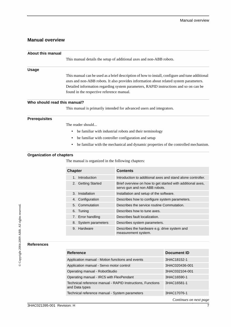
Organization of chapters
The manual is organized in the following chapters:
References
Chapter Contents
1. Introduction Introduction to additional axes and stand alone controller.
2. Getting Started Brief overview on how to get started with additional axes, servo gun and non ABB robots.
3. Installation Installation and setup of the software.
4. Configuration Describes how to configure system parameters.
5. Commutation Describes the service routine Commutation.
6. Tuning Describes how to tune axes.
7. Error handling Describes fault localization.
8. System parameters Describes system parameters.
9. Hardware Describes the hardware e.g. drive system and measurement system.
Reference Document ID
Application manual - Motion functions and events 3HAC18152-1
Application manual - Servo motor control 3HAC020436-001
Operating manual - RobotStudio 3HAC032104-001
Operating manual - IRC5 with FlexPendant 3HAC16590-1
Technical reference manual - RAPID Instructions, Functions and Data types
3HAC16581-1
Technical reference manual - System parameters 3HAC17076-1
Continues on next page
Manual overview
3HAC021395-001 Revision: H8
© C
opyr
ight
200
4-20
09 A
BB
. All
righ
ts r
eser
ved.
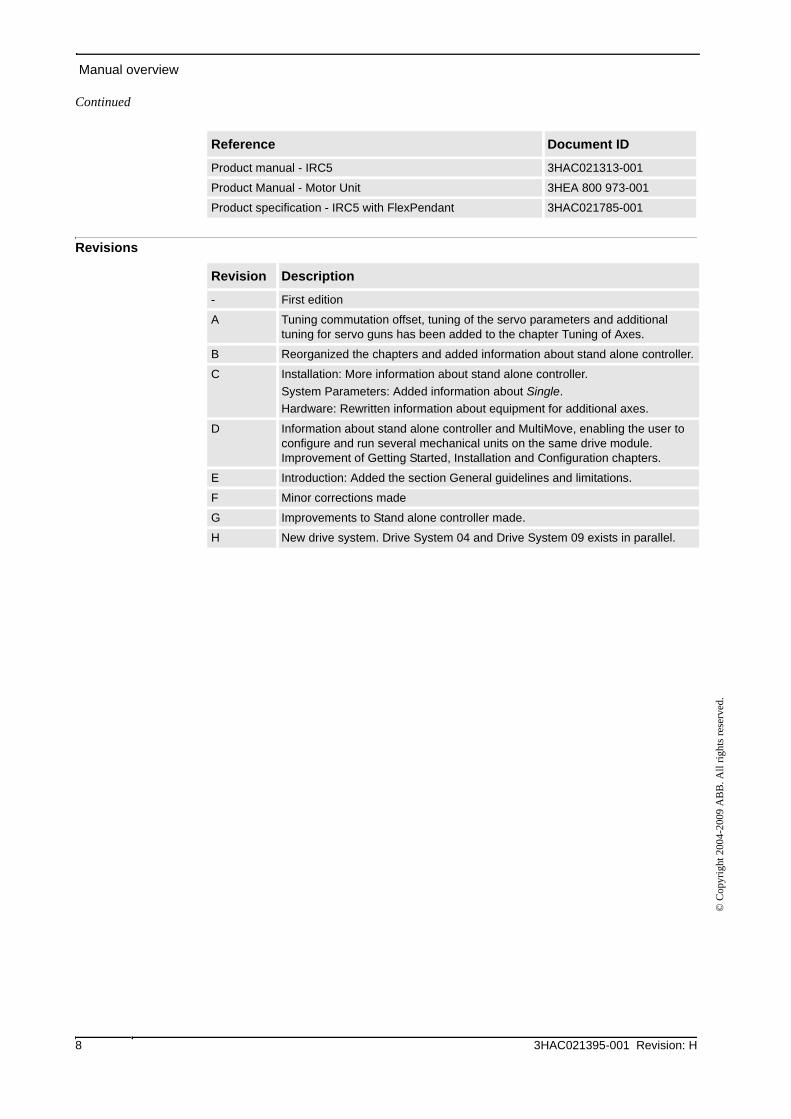
Revisions
Product manual - IRC5 3HAC021313-001
Product Manual - Motor Unit 3HEA 800 973-001
Product specification - IRC5 with FlexPendant 3HAC021785-001
Reference Document ID
Revision Description
- First edition
A Tuning commutation offset, tuning of the servo parameters and additional tuning for servo guns has been added to the chapter Tuning of Axes.
B Reorganized the chapters and added information about stand alone controller.
C Installation: More information about stand alone controller.
System Parameters: Added information about Single.
Hardware: Rewritten information about equipment for additional axes.
D Information about stand alone controller and MultiMove, enabling the user to configure and run several mechanical units on the same drive module. Improvement of Getting Started, Installation and Configuration chapters.
E Introduction: Added the section General guidelines and limitations.
F Minor corrections made
G Improvements to Stand alone controller made.
H New drive system. Drive System 04 and Drive System 09 exists in parallel.
Continued
Product documentation, M2004
93HAC021395-001 Revision: H
© C
opyr
ight
200
4-20
09 A
BB
. All
righ
ts r
eser
ved.
Product documentation, M2004
General
The robot documentation is divided into a number of categories. This listing is based on the
type of information contained within the documents, regardless of whether the products are
standard or optional. This means that any given delivery of robot products will not contain all documents listed, only the ones pertaining to the equipment delivered.
However, all documents listed may be ordered from ABB. The documents listed are valid for
M2004 robot systems.
Product manuals
All hardware, robots and controllers, will be delivered with a Product manual that contains:
• Safety information
• Installation and commissioning (descriptions of mechanical installation, electrical
connections)
• Maintenance (descriptions of all required preventive maintenance procedures
including intervals)
• Repair (descriptions of all recommended repair procedures including spare parts)
• Additional procedures, if any (calibration, decommissioning)
• Reference information (article numbers for documentation referred to in Product
manual, procedures, lists of tools, safety standards)
• Part list
• Foldouts or exploded views
• Circuit diagrams
Technical reference manuals
The following manuals describe the robot software in general and contain relevant reference
information:
• RAPID Overview: An overview of the RAPID programming language.
• RAPID Instructions, Functions and Data types: Description and syntax for all
RAPID instructions, functions and data types.
• System parameters: Description of system parameters and configuration workflows.
Application manuals
Specific applications (for example software or hardware options) are described in
Application manuals. An application manual can describe one or several applications.
An application manual generally contains information about:
• The purpose of the application (what it does and when it is useful)
• What is included (for example cables, I/O boards, RAPID instructions, system
parameters, CD with PC software)
• How to use the application
• Examples of how to use the application
Continues on next page
Product documentation, M2004
3HAC021395-001 Revision: H10
© C
opyr
ight
200
4-20
09 A
BB
. All
righ
ts r
eser
ved.
Operating manuals
This group of manuals is aimed at those having first hand operational contact with the robot,
that is production cell operators, programmers and trouble shooters. The group of manuals
includes:
• Emergency safety information
• General safety information
• Getting started, IRC5
• IRC5 with FlexPendant
• RobotStudio
• Introduction to RAPID
• Trouble shooting, for the controller and robot
Continued
Safety
113HAC021395-001 Revision: H
© C
opyr
ight
200
4-20
09 A
BB
. All
righ
ts r
eser
ved.
Safety
Safety of personnel
A robot is heavy and extremely powerful regardless of its speed. A pause or long stop in
movement can be followed by a fast hazardous movement. Even if a pattern of movement is
predicted, a change in operation can be triggered by an external signal resulting in an
unexpected movement.
Therefore, it is important that all safety regulations are followed when entering safeguarded
space.
Safety regulations
Before beginning work with the robot, make sure you are familiar with the safety regulations
described in the manual General safety information.

Safety
3HAC021395-001 Revision: H12
© C
opyr
ight
200
4-20
09 A
BB
. All
righ
ts r
eser
ved.
1 Introduction
1.1. Overview
133HAC021395-001 Revision: H
© C
opyr
ight
200
4-20
09 A
BB
. All
righ
ts r
eser
ved.
1 Introduction
1.1. Overview
Purpose
The additional axes option is used when the robot controller needs to control additional axes
besides the robot axes. These axes are synchronized and, if desired, coordinated with the
movement of the robot, which results in high speed and high accuracy.
Stand alone controller is an ABB controller delivered without an ABB robot. The purpose is
to use it to control non-ABB equipment.
When the controller is used in a robot system with external axes or a non-ABB manipulator,
the system requires configuration and tuning as detailed in this manual. This manual can also
be useful when such a system needs to be upgraded.
As external axes and non-ABB robots consume more power the drive system needs a more
powerful transformer, rectifier and capacitor. In addition, suitable drive units must be
installed in the controller. The hardware setup must also be configured with software to make
the system functional.
Basic approach
This is the basic approach for the setup of additional axes or a stand alone controller.
• Installation
• Configuration
• Tuning
For a detailed description of how this is done, see the respective section.
For more information on the hardware components see Hardware on page 181.
WARNING!
The manual mode peripheral speed of the external axis must be restricted to 250 mm/s for
personal safety reasons. The speed is supervised at three different levels, which means that
three system parameters need to be set up. For more information see Limit peripheral speed
of external axis on page 69.
1 Introduction
1.2. Definitions
3HAC021395-001 Revision: H14
© C
opyr
ight
200
4-20
09 A
BB
. All
righ
ts r
eser
ved.
1.2. Definitions
Robot
A robot is a mechanical unit with a tool center point (TCP). A robot can be programmed both
in Cartesian coordinates (x, y and z) of the TCP and in tool orientation.
Non-MultiMove system
A non-MultiMove system can have
• only one motion task
• only one robot
• up to 6 additional axes (which can be grouped in an arbitrary number of mechanical
units)
• up to 12 axes in total (located in one or two drive modules)
TIP!
In a non-MultiMove system, semi-independent programming of individual mechanical units
or axes can be achieved through the option Independent Axes. However, MultiMove is
normally preferred when independent programming is desired.
MultiMove system
A MultiMove system can have
• up to 6 motion tasks (each task has the same limitations as in a non-MultiMove
system)
• up to 4 robots
• up to 4 drive modules (i.e. up to 36 axes including the robot axes)
Additional axes
The robot controller can control additional axes besides the robot axes. These mechanical
units can be used for Non-MultiMove and MultiMove systems alike. They can be jogged and
coordinated with the movements of the robot. The system may have a single additional axis,
e.g. a motor, or a set of additional axes such as a two axis positioner.
Stand alone controller
Stand alone controller means an ABB controller delivered without an ABB robot. The stand
alone controller can be used to control non-ABB equipment, usually TCP robots. It can be
used for Non-MultiMove and MultiMove systems alike. MultiMove makes it possible to
configure and run multiple mechanical units on the same drive module.
1 Introduction
1.3. General guidelines and limitations
153HAC021395-001 Revision: H
© C
opyr
ight
200
4-20
09 A
BB
. All
righ
ts r
eser
ved.
1.3. General guidelines and limitations
Use integer gear ratio
The transmission gear ratio between motor and arm of a continuously rotating axis shall be
an integer in order not to cause calibration problems when updating revolution counters.
When the revolution counter is updated, the number of motor revolutions is reset. In order for
the zero position of the motor to coincide with the zero position of the arm, independent of
number of revolutions on the arm side, the gear ratio needs to be an integer (not a decimal
number).
Example: Gear ratio = 1:81 (not 1:81.73).
This problem will only be visible when updating revolution counters with the arm side rotated
n turns from the original zero position. I.e. an axis with mechanical stops will not have this
problem.

1 Introduction
1.3. General guidelines and limitations
3HAC021395-001 Revision: H16
© C
opyr
ight
200
4-20
09 A
BB
. All
righ
ts r
eser
ved.
2 Getting started
2.1. Get started with additional axes, servo guns and non-ABB robots
173HAC021395-001 Revision: H
© C
opyr
ight
200
4-20
09 A
BB
. All
righ
ts r
eser
ved.
2 Getting started
2.1. Get started with additional axes, servo guns and non-ABB robots
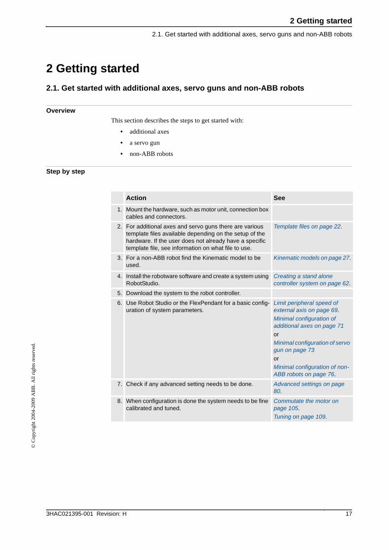
Overview
This section describes the steps to get started with:
• additional axes
• a servo gun
• non-ABB robots
Step by step
Action See
1. Mount the hardware, such as motor unit, connection box cables and connectors.
2. For additional axes and servo guns there are various template files available depending on the setup of the hardware. If the user does not already have a specific template file, see information on what file to use.
Template files on page 22.
3. For a non-ABB robot find the Kinematic model to be used.
Kinematic models on page 27.
4. Install the robotware software and create a system using RobotStudio.
Creating a stand alone controller system on page 62.
5. Download the system to the robot controller.
6. Use Robot Studio or the FlexPendant for a basic config-uration of system parameters.
Limit peripheral speed of external axis on page 69.
Minimal configuration of additional axes on page 71
or
Minimal configuration of servo gun on page 73
or
Minimal configuration of non-ABB robots on page 76.
7. Check if any advanced setting needs to be done. Advanced settings on page 80.
8. When configuration is done the system needs to be fine calibrated and tuned.
Commutate the motor on page 105.
Tuning on page 109.

2 Getting started
2.1. Get started with additional axes, servo guns and non-ABB robots
3HAC021395-001 Revision: H18
© C
opyr
ight
200
4-20
09 A
BB
. All
righ
ts r
eser
ved.
3 Installation
3.1.1. Standard additional axis (Option selected)
193HAC021395-001 Revision: H
© C
opyr
ight
200
4-20
09 A
BB
. All
righ
ts r
eser
ved.
3 Installation
3.1 Additional axes and servo guns
3.1.1. Standard additional axis (Option selected)
Overview
Normally all necessary configuration parameters regarding drive unit, rectifiers and
transformers are pre-loaded at ABB, and do not need to be re-installed. For more information
on how to add options to the system, see Operating manual - RobotStudio.
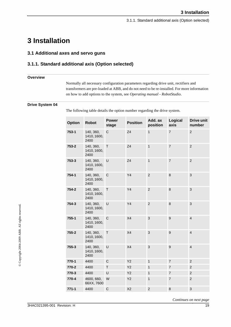
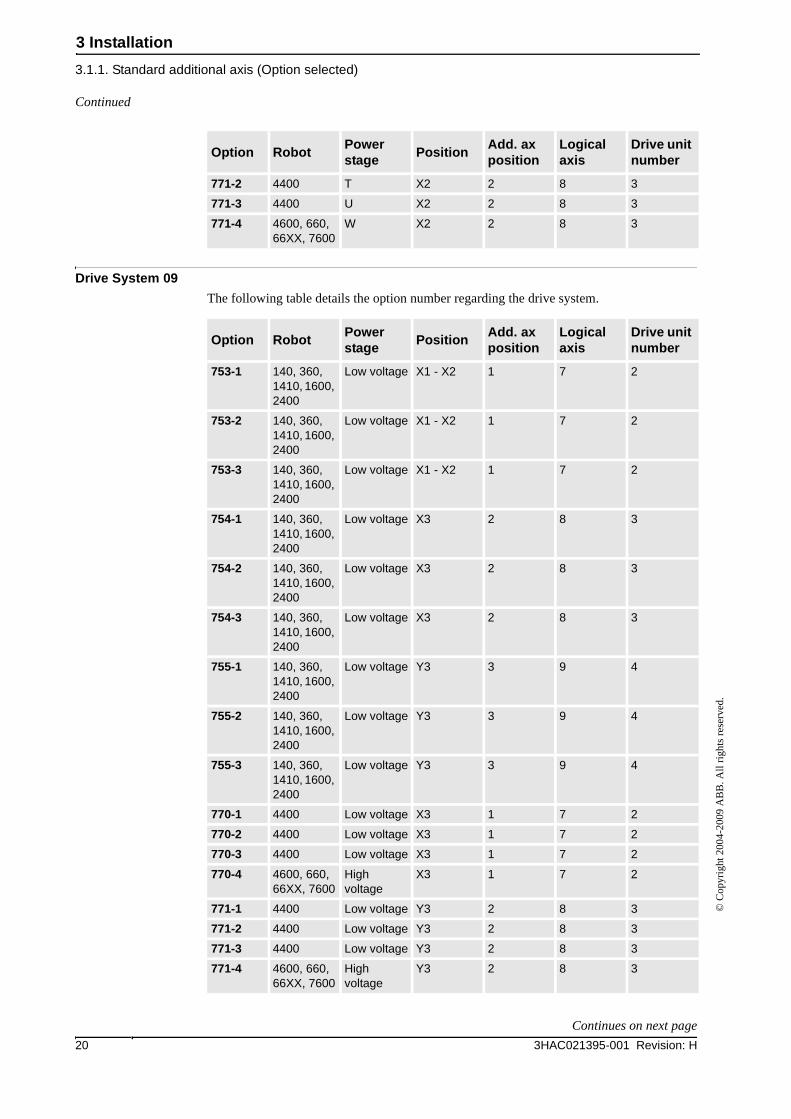
Drive System 04
The following table details the option number regarding the drive system.
Option RobotPower stage
PositionAdd. ax position
Logical axis
Drive unit number
753-1 140, 360, 1410, 1600, 2400
C Z4 1 7 2
753-2 140, 360, 1410, 1600, 2400
T Z4 1 7 2
753-3 140, 360, 1410, 1600, 2400
U Z4 1 7 2
754-1 140, 360, 1410, 1600, 2400
C Y4 2 8 3
754-2 140, 360, 1410, 1600, 2400
T Y4 2 8 3
754-3 140, 360, 1410, 1600, 2400
U Y4 2 8 3
755-1 140, 360, 1410, 1600, 2400
C X4 3 9 4
755-2 140, 360, 1410, 1600, 2400
T X4 3 9 4
755-3 140, 360, 1410, 1600, 2400
U X4 3 9 4
770-1 4400 C Y2 1 7 2
770-2 4400 T Y2 1 7 2
770-3 4400 U Y2 1 7 2
770-4 4600, 660, 66XX, 7600
W Y2 1 7 2
771-1 4400 C X2 2 8 3
Continues on next page
3 Installation
3.1.1. Standard additional axis (Option selected)
3HAC021395-001 Revision: H20
© C
opyr
ight
200
4-20
09 A
BB
. All
righ
ts r
eser
ved.
Drive System 09
The following table details the option number regarding the drive system.
771-2 4400 T X2 2 8 3
771-3 4400 U X2 2 8 3
771-4 4600, 660, 66XX, 7600
W X2 2 8 3
Option RobotPower stage
PositionAdd. ax position
Logical axis
Drive unit number
Option RobotPower stage
PositionAdd. ax position
Logical axis
Drive unit number
753-1 140, 360, 1410, 1600, 2400
Low voltage X1 - X2 1 7 2
753-2 140, 360, 1410, 1600, 2400
Low voltage X1 - X2 1 7 2
753-3 140, 360, 1410, 1600, 2400
Low voltage X1 - X2 1 7 2
754-1 140, 360, 1410, 1600, 2400
Low voltage X3 2 8 3
754-2 140, 360, 1410, 1600, 2400
Low voltage X3 2 8 3
754-3 140, 360, 1410, 1600, 2400
Low voltage X3 2 8 3
755-1 140, 360, 1410, 1600, 2400
Low voltage Y3 3 9 4
755-2 140, 360, 1410, 1600, 2400
Low voltage Y3 3 9 4
755-3 140, 360, 1410, 1600, 2400
Low voltage Y3 3 9 4
770-1 4400 Low voltage X3 1 7 2
770-2 4400 Low voltage X3 1 7 2
770-3 4400 Low voltage X3 1 7 2
770-4 4600, 660, 66XX, 7600
High voltage
X3 1 7 2
771-1 4400 Low voltage Y3 2 8 3
771-2 4400 Low voltage Y3 2 8 3
771-3 4400 Low voltage Y3 2 8 3
771-4 4600, 660, 66XX, 7600
High voltage
Y3 2 8 3
Continued
Continues on next page
3 Installation
3.1.1. Standard additional axis (Option selected)
213HAC021395-001 Revision: H
© C
opyr
ight
200
4-20
09 A
BB
. All
righ
ts r
eser
ved.
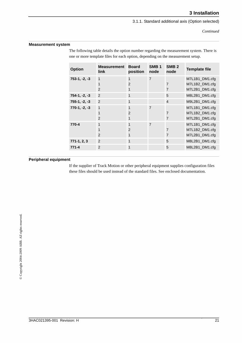
Measurement system
The following table details the option number regarding the measurement system. There is
one or more template files for each option, depending on the measurement setup.
Peripheral equipment
If the supplier of Track Motion or other peripheral equipment supplies configuration files
these files should be used instead of the standard files. See enclosed documentation.
OptionMeasurement link
Board position
SMB 1 node
SMB 2 node
Template file
753-1, -2, -3 1
1
2
1
2
1
7
7
7
M7L1B1_DM1.cfg
M7L1B2_DM1.cfg
M7L2B1_DM1.cfg
754-1, -2, -3 2 1 5 M8L2B1_DM1.cfg
755-1, -2, -3 2 1 4 M9L2B1_DM1.cfg
770-1, -2, -3 1
1
2
1
2
1
7
7
7
M7L1B1_DM1.cfg
M7L1B2_DM1.cfg
M7L2B1_DM1.cfg
770-4 1
1
2
1
2
1
7
7
7
M7L1B1_DM1.cfg
M7L1B2_DM1.cfg
M7L2B1_DM1.cfg
771-1, 2, 3 2 1 5 M8L2B1_DM1.cfg
771-4 2 1 5 M8L2B1_DM1.cfg
Continued
3 Installation
3.1.2. Template files
3HAC021395-001 Revision: H22
© C
opyr
ight
200
4-20
09 A
BB
. All
righ
ts r
eser
ved.
3.1.2. Template files
Overview
This section details the template files for respective hardware. Normally you only need to
change the motor data in these files. For more information on how to change these files, see
Operating manual - RobotStudio. The files are located in the directory
Mediapool\RobotWare_5.XX.XXXX\Utility\AdditionalAxis. They can also be
found in the stand alone controller package.
NOTE!
For Drive System 04, there is no drive unit place 9 on large robots, (IRB 4400, 6600, 6650
and 7600).
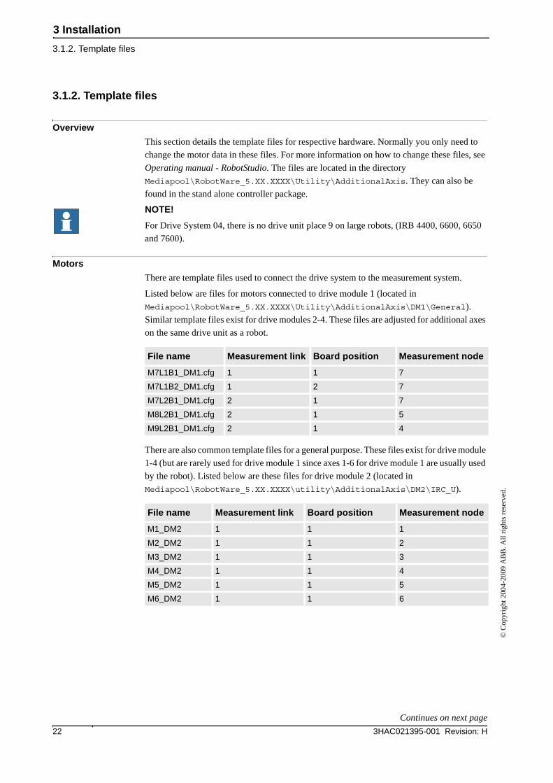
Motors
There are template files used to connect the drive system to the measurement system.
Listed below are files for motors connected to drive module 1 (located in
Mediapool\RobotWare_5.XX.XXXX\Utility\AdditionalAxis\DM1\General).
Similar template files exist for drive modules 2-4. These files are adjusted for additional axes
on the same drive unit as a robot.
There are also common template files for a general purpose. These files exist for drive module
1-4 (but are rarely used for drive module 1 since axes 1-6 for drive module 1 are usually used
by the robot). Listed below are these files for drive module 2 (located in
Mediapool\RobotWare_5.XX.XXXX\utility\AdditionalAxis\DM2\IRC_U).
File name Measurement link Board position Measurement node
M7L1B1_DM1.cfg 1 1 7
M7L1B2_DM1.cfg 1 2 7
M7L2B1_DM1.cfg 2 1 7
M8L2B1_DM1.cfg 2 1 5
M9L2B1_DM1.cfg 2 1 4
File name Measurement link Board position Measurement node
M1_DM2 1 1 1
M2_DM2 1 1 2
M3_DM2 1 1 3
M4_DM2 1 1 4
M5_DM2 1 1 5
M6_DM2 1 1 6
Continues on next page
3 Installation
3.1.2. Template files
233HAC021395-001 Revision: H
© C
opyr
ight
200
4-20
09 A
BB
. All
righ
ts r
eser
ved.
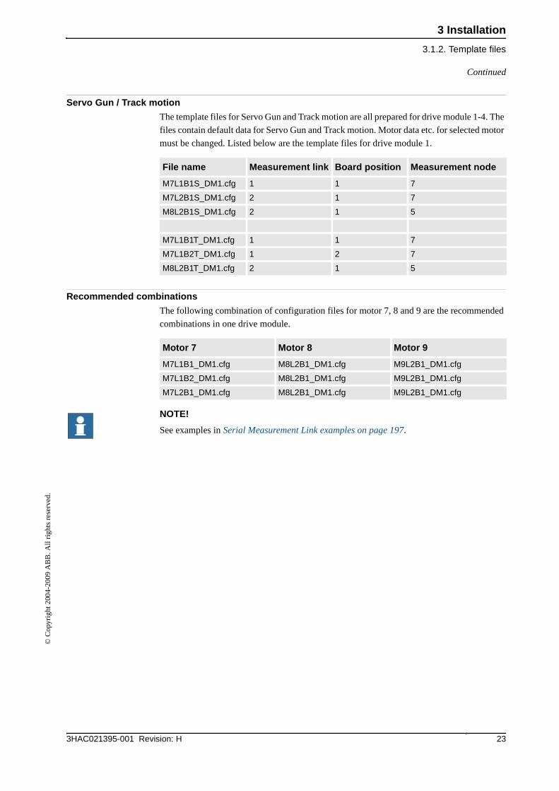
Servo Gun / Track motion
The template files for Servo Gun and Track motion are all prepared for drive module 1-4. The
files contain default data for Servo Gun and Track motion. Motor data etc. for selected motor
must be changed. Listed below are the template files for drive module 1.
Recommended combinations
The following combination of configuration files for motor 7, 8 and 9 are the recommended
combinations in one drive module.
NOTE!
See examples in Serial Measurement Link examples on page 197.
File name Measurement link Board position Measurement node
M7L1B1S_DM1.cfg 1 1 7
M7L2B1S_DM1.cfg 2 1 7
M8L2B1S_DM1.cfg 2 1 5
M7L1B1T_DM1.cfg 1 1 7
M7L1B2T_DM1.cfg 1 2 7
M8L2B1T_DM1.cfg 2 1 5
Motor 7 Motor 8 Motor 9
M7L1B1_DM1.cfg M8L2B1_DM1.cfg M9L2B1_DM1.cfg
M7L1B2_DM1.cfg M8L2B1_DM1.cfg M9L2B1_DM1.cfg
M7L2B1_DM1.cfg M8L2B1_DM1.cfg M9L2B1_DM1.cfg
Continued
3 Installation
3.1.3. Serial measurement system configuration
3HAC021395-001 Revision: H24
© C
opyr
ight
200
4-20
09 A
BB
. All
righ
ts r
eser
ved.
3.1.3. Serial measurement system configuration
Overview
The following section details how to configure the measurement link.
Measurement Channel
The Measurement Channel parameters can easily be changed via RobotStudio or the
FlexPendant. Select the configuration topic Motion and the type Measurement Channel.
Another alternative is to edit the parameters in the file MOC.cfg and load this file to the
controller. For information about how to load a cfg file, see Operating manual - RobotStudio.
NOTE!
Each node (1 to 7) must not be used more than once on each serial measurement link.
Action Info/Illustration
1. Select the serial measurement link by changing the value of the parameter measurement_link.
selectable values: 1 or 2
2. Select the SMB placement by changing the value of the parameter board_position.
selectable values: 1 or 2
3. Select the measurement node by changing the value of the parameter measurement_node.
selectable values: 1 to 7
3 Installation
3.2.1. Introduction
253HAC021395-001 Revision: H
© C
opyr
ight
200
4-20
09 A
BB
. All
righ
ts r
eser
ved.
3.2 Non ABB robots
3.2.1. Introduction
Overview
This section details how to create and install a stand alone controller system, i.e. a system to
be used with non-ABB robots. The basic steps to do this are as follows:
• Find the correct drive unit configuration.
• Find the appropriate kinematic model.
• Install RobotWare and the stand alone controller software on your PC.
• Create a stand alone controller system with the selected kinematic model.
• Download the system to the robot controller.
This section also details how to modify and distribute a stand alone package for easy
installation and startup at a customer.
3 Installation
3.2.2. Drive module for non-ABB robots
3HAC021395-001 Revision: H26
© C
opyr
ight
200
4-20
09 A
BB
. All
righ
ts r
eser
ved.
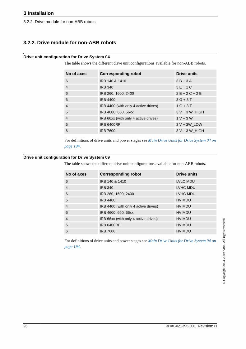
3.2.2. Drive module for non-ABB robots
Drive unit configuration for Drive System 04
The table shows the different drive unit configurations available for non-ABB robots.
For definitions of drive units and power stages see Main Drive Units for Drive System 04 on
page 194.
Drive unit configuration for Drive System 09
The table shows the different drive unit configurations available for non-ABB robots.
For definitions of drive units and power stages see Main Drive Units for Drive System 04 on
page 194.
No of axes Corresponding robot Drive units
6 IRB 140 & 1410 3 B + 3 A
4 IRB 340 3 E + 1 C
6 IRB 260, 1600, 2400 2 E + 2 C + 2 B
6 IRB 4400 3 G + 3 T
4 IRB 4400 (with only 4 active drives) 1 G + 3 T
6 IRB 4600, 660, 66xx 3 V + 3 W_HIGH
4 IRB 66xx (with only 4 active drives) 1 V + 3 W
6 IRB 6400RF 3 V + 3W_LOW
6 IRB 7600 3 V + 3 W_HIGH
No of axes Corresponding robot Drive units
6 IRB 140 & 1410 LVLC MDU
4 IRB 340 LVHC MDU
6 IRB 260, 1600, 2400 LVHC MDU
6 IRB 4400 HV MDU
4 IRB 4400 (with only 4 active drives) HV MDU
6 IRB 4600, 660, 66xx HV MDU
4 IRB 66xx (with only 4 active drives) HV MDU
6 IRB 6400RF HV MDU
6 IRB 7600 HV MDU
3 Installation
3.2.3.1. Introduction
273HAC021395-001 Revision: H
© C
opyr
ight
200
4-20
09 A
BB
. All
righ
ts r
eser
ved.
3.2.3. Kinematic models
3.2.3.1. Introduction
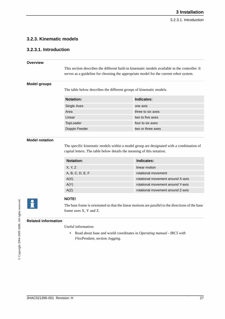
Overview
This section describes the different built-in kinematic models available in the controller. It
serves as a guideline for choosing the appropriate model for the current robot system.
Model groups
The table below describes the different groups of kinematic models.
Model notation
The specific kinematic models within a model group are designated with a combination of
capital letters. The table below details the meaning of this notation.
NOTE!
The base frame is orientated so that the linear motions are parallel to the directions of the base
frame axes X, Y and Z.
Related information
Useful information:
• Read about base and world coordinates in Operating manual - IRC5 with
FlexPendant, section Jogging.
Notation: Indicates:
Single Axes one axis
Area three to six axes
Linear two to five axes
TopLoader four to six axes
Doppin Feeder two or three axes
Notation: Indicates:
X, Y, Z linear motion
A, B, C, D, E, F rotational movement
A(X) rotational movement around X-axis
A(Y) rotational movement around Y-axis
A(Z) rotational movement around Z-axis
3 Installation
3.2.3.2. Kinematic model XYZ
3HAC021395-001 Revision: H28
© C
opyr
ight
200
4-20
09 A
BB
. All
righ
ts r
eser
ved.
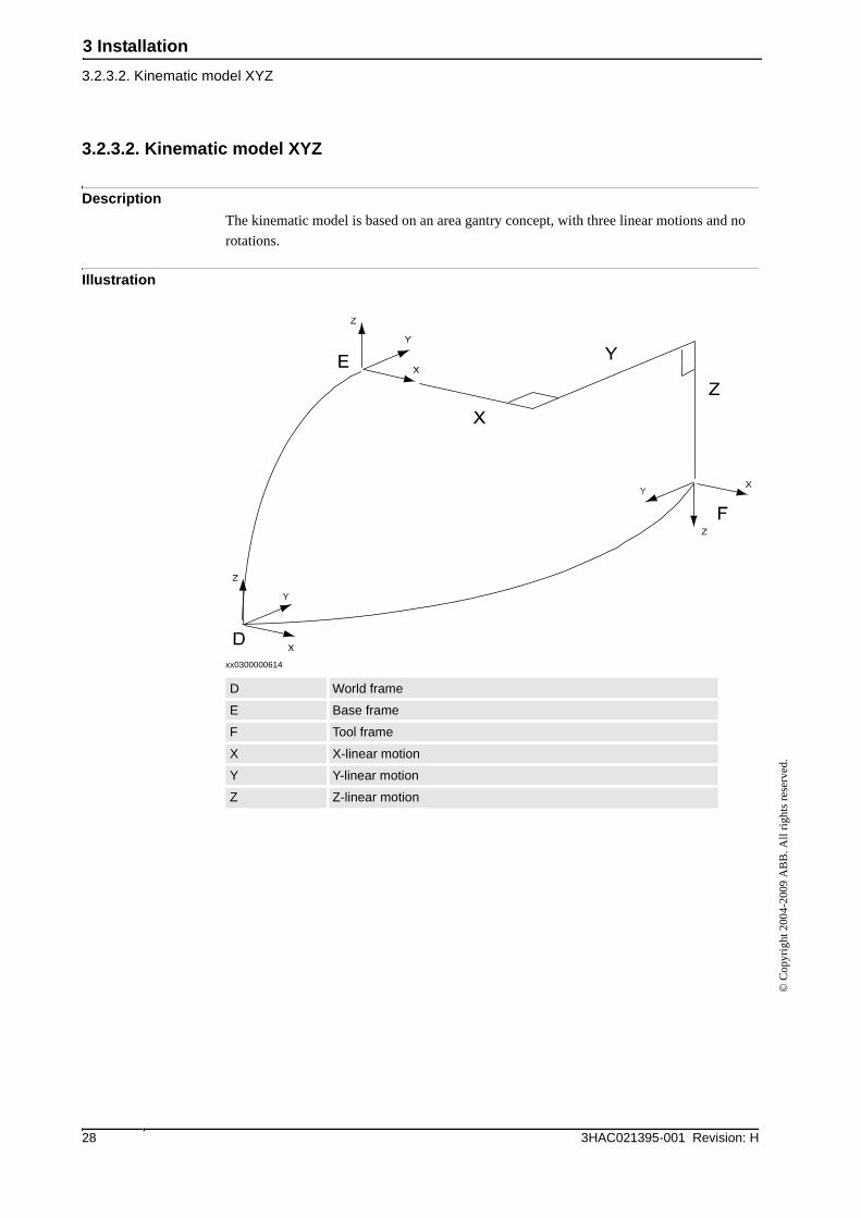
3.2.3.2. Kinematic model XYZ
Description
The kinematic model is based on an area gantry concept, with three linear motions and no
rotations.
Illustration
xx0300000614
D World frame
E Base frame
F Tool frame
X X-linear motion
Y Y-linear motion
Z Z-linear motion
3 Installation
3.2.3.3. Kinematic model C(Z)
293HAC021395-001 Revision: H
© C
opyr
ight
200
4-20
09 A
BB
. All
righ
ts r
eser
ved.
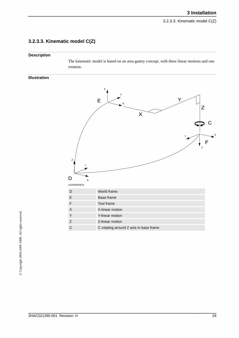
3.2.3.3. Kinematic model C(Z)
Description
The kinematic model is based on an area gantry concept, with three linear motions and one
rotation.
Illustration
xx0300000616
D World frame
E Base frame
F Tool frame
X X-linear motion
Y Y-linear motion
Z Z-linear motion
C C rotating around Z axis in base frame
3 Installation
3.2.3.4. Kinematic model B(X)
3HAC021395-001 Revision: H30
© C
opyr
ight
200
4-20
09 A
BB
. All
righ
ts r
eser
ved.
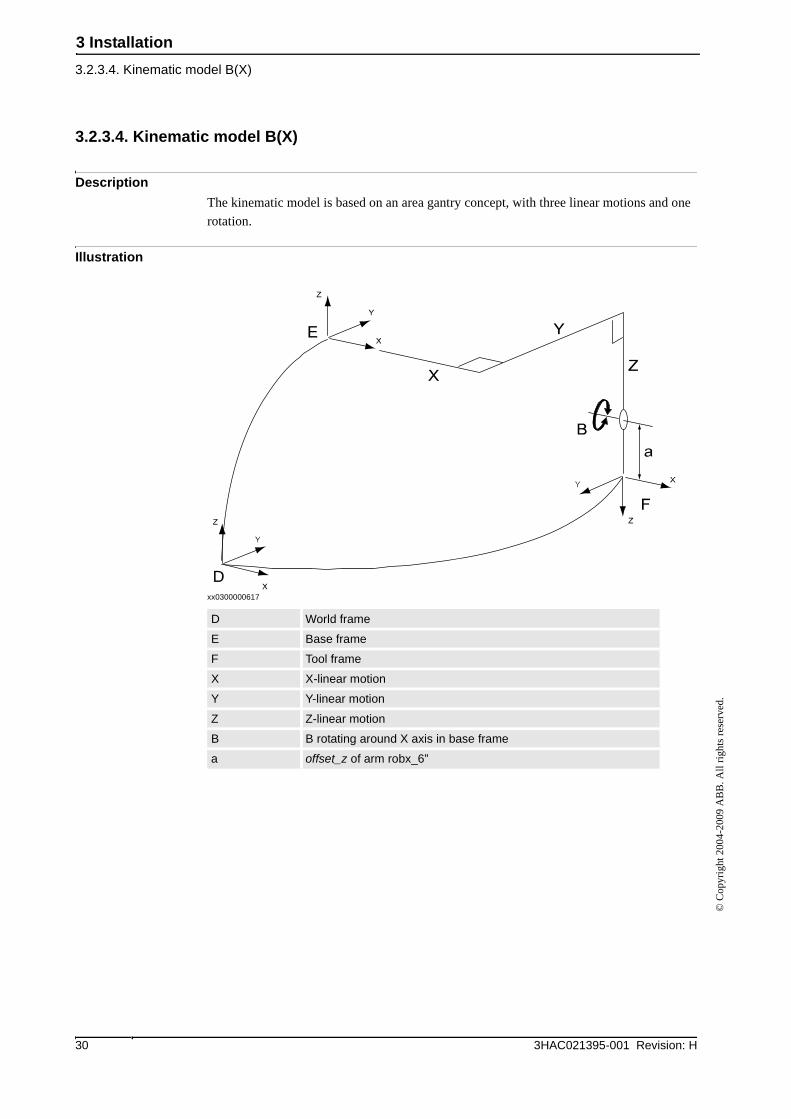
3.2.3.4. Kinematic model B(X)
Description
The kinematic model is based on an area gantry concept, with three linear motions and one
rotation.
Illustration
xx0300000617
D World frame
E Base frame
F Tool frame
X X-linear motion
Y Y-linear motion
Z Z-linear motion
B B rotating around X axis in base frame
a offset_z of arm robx_6”
3 Installation
3.2.3.5. Kinematic model XYZB(Y)
313HAC021395-001 Revision: H
© C
opyr
ight
200
4-20
09 A
BB
. All
righ
ts r
eser
ved.
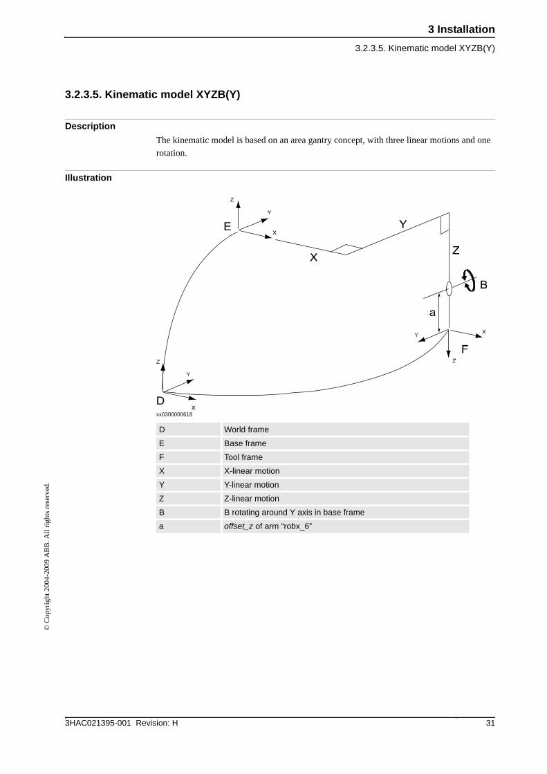
3.2.3.5. Kinematic model XYZB(Y)
Description
The kinematic model is based on an area gantry concept, with three linear motions and one
rotation.
Illustration
xx0300000618
D World frame
E Base frame
F Tool frame
X X-linear motion
Y Y-linear motion
Z Z-linear motion
B B rotating around Y axis in base frame
a offset_z of arm “robx_6”
3 Installation
3.2.3.6. Kinematic model XYZC(Z)B(X)
3HAC021395-001 Revision: H32
© C
opyr
ight
200
4-20
09 A
BB
. All
righ
ts r
eser
ved.
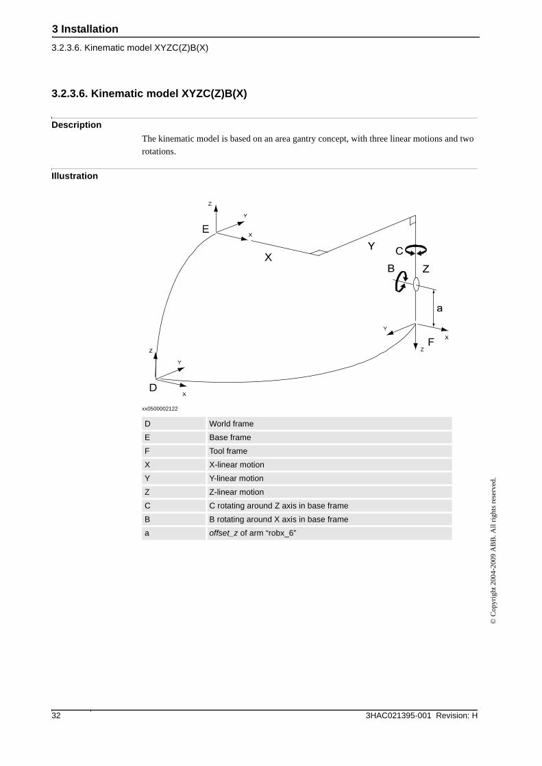
3.2.3.6. Kinematic model XYZC(Z)B(X)
Description
The kinematic model is based on an area gantry concept, with three linear motions and two
rotations.
Illustration
xx0500002122
D World frame
E Base frame
F Tool frame
X X-linear motion
Y Y-linear motion
Z Z-linear motion
C C rotating around Z axis in base frame
B B rotating around X axis in base frame
a offset_z of arm “robx_6”

3 Installation
3.2.3.7. Kinematic model XYZC(Z)B(Y)
333HAC021395-001 Revision: H
© C
opyr
ight
200
4-20
09 A
BB
. All
righ
ts r
eser
ved.
3.2.3.7. Kinematic model XYZC(Z)B(Y)
Description
The kinematic model is based on an area gantry concept, with three linear motions and two
rotations.
Illustration
xx0500002122
D World Frame
E Base Frame
F Tool Frame
X X-linear motion
Y Y-linear motion
Z Z-linear motion
C C rotating around Z axis in base frame
B B rotating around Y axis in base frame
a offset_z of arm robx_6
3 Installation
3.2.3.8. Kinematic model XYZB(X)A(Z)
3HAC021395-001 Revision: H34
© C
opyr
ight
200
4-20
09 A
BB
. All
righ
ts r
eser
ved.
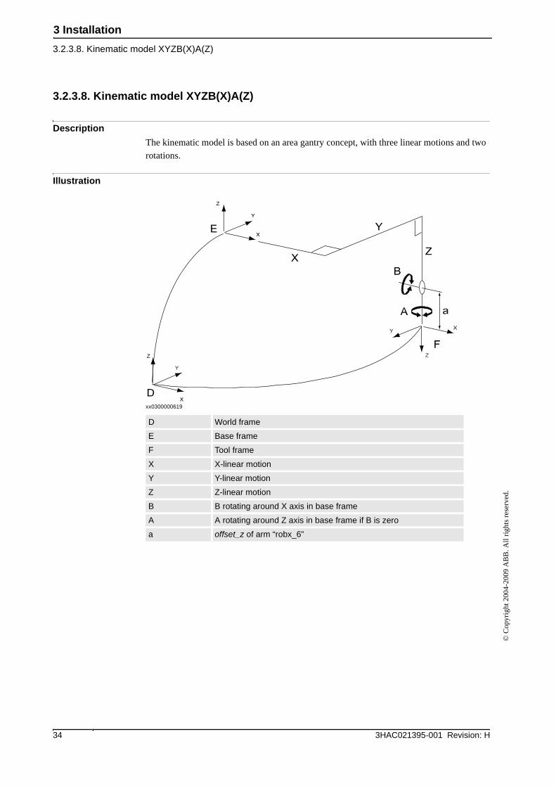
3.2.3.8. Kinematic model XYZB(X)A(Z)
Description
The kinematic model is based on an area gantry concept, with three linear motions and two
rotations.
Illustration
xx0300000619
D World frame
E Base frame
F Tool frame
X X-linear motion
Y Y-linear motion
Z Z-linear motion
B B rotating around X axis in base frame
A A rotating around Z axis in base frame if B is zero
a offset_z of arm “robx_6”
3 Installation
3.2.3.9. Kinematic model XYZB(Y)A(Z)
353HAC021395-001 Revision: H
© C
opyr
ight
200
4-20
09 A
BB
. All
righ
ts r
eser
ved.
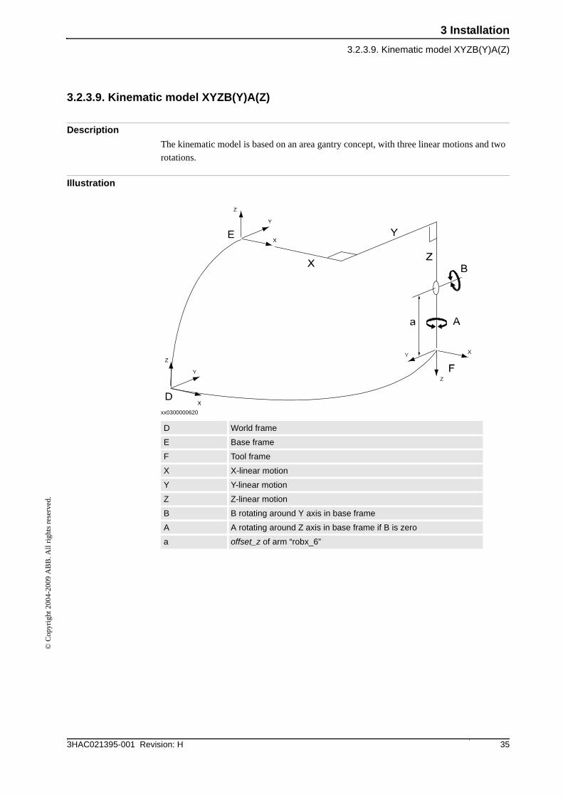
3.2.3.9. Kinematic model XYZB(Y)A(Z)
Description
The kinematic model is based on an area gantry concept, with three linear motions and two
rotations.
Illustration
xx0300000620
D World frame
E Base frame
F Tool frame
X X-linear motion
Y Y-linear motion
Z Z-linear motion
B B rotating around Y axis in base frame
A A rotating around Z axis in base frame if B is zero
a offset_z of arm “robx_6”
3 Installation
3.2.3.10. Kinematic model XYZC(Z)B(X)A(Z)
3HAC021395-001 Revision: H36
© C
opyr
ight
200
4-20
09 A
BB
. All
righ
ts r
eser
ved.
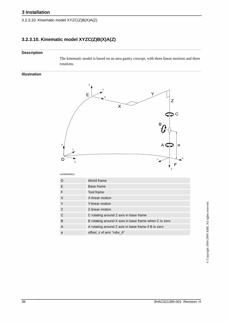
3.2.3.10. Kinematic model XYZC(Z)B(X)A(Z)
Description
The kinematic model is based on an area gantry concept, with three linear motions and three
rotations.
Illustration
xx0300000621
D World frame
E Base frame
F Tool frame
X X-linear motion
Y Y-linear motion
Z Z-linear motion
C C rotating around Z axis in base frame
B B rotating around X axis in base frame when C is zero
A A rotating around Z axis in base frame if B is zero
a offset_z of arm “robx_6”
3 Installation
3.2.3.11. Kinematic model XYZC(Z)B(Y)A(Z)
373HAC021395-001 Revision: H
© C
opyr
ight
200
4-20
09 A
BB
. All
righ
ts r
eser
ved.
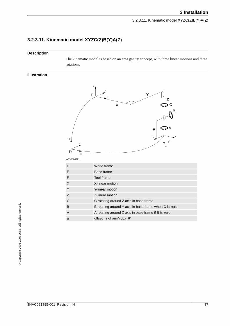
3.2.3.11. Kinematic model XYZC(Z)B(Y)A(Z)
Description
The kinematic model is based on an area gantry concept, with three linear motions and three
rotations.
Illustration
xx0500002211
D World frame
E Base frame
F Tool frame
X X-linear motion
Y Y-linear motion
Z Z-linear motion
C C rotating around Z axis in base frame
B B rotating around Y axis in base frame when C is zero
A A rotating around Z axis in base frame if B is zero
a offset _z of arm”robx_6”
3 Installation
3.2.3.12. Kinematic model XYZC(Z)A(X)
3HAC021395-001 Revision: H38
© C
opyr
ight
200
4-20
09 A
BB
. All
righ
ts r
eser
ved.
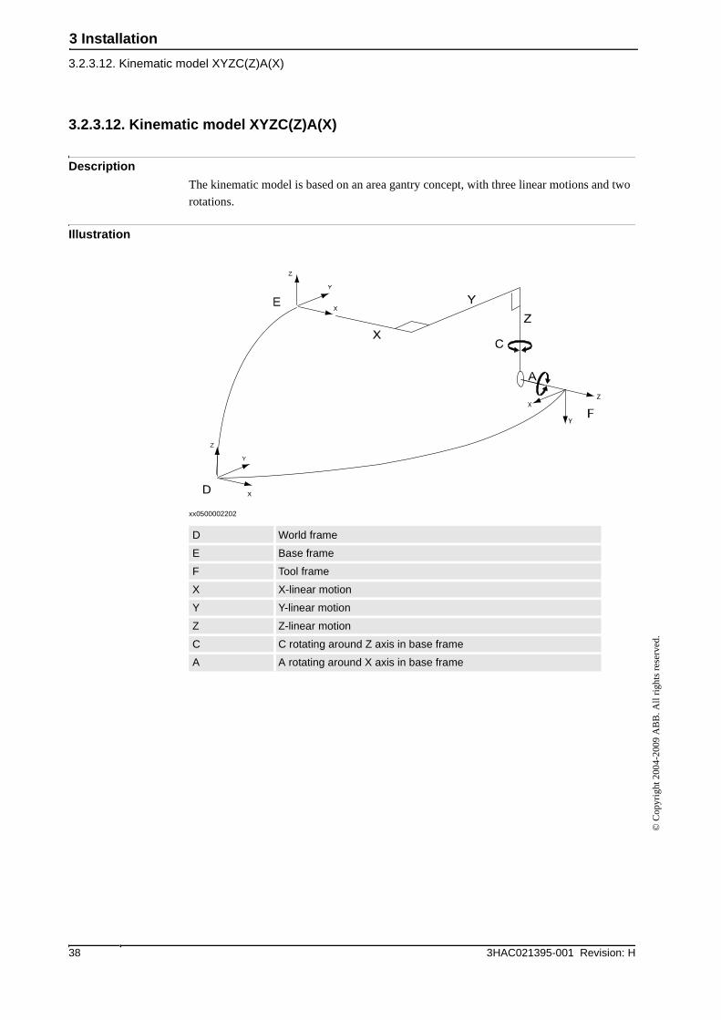
3.2.3.12. Kinematic model XYZC(Z)A(X)
Description
The kinematic model is based on an area gantry concept, with three linear motions and two
rotations.
Illustration
xx0500002202
D World frame
E Base frame
F Tool frame
X X-linear motion
Y Y-linear motion
Z Z-linear motion
C C rotating around Z axis in base frame
A A rotating around X axis in base frame
3 Installation
3.2.3.13. Kinematic model XYZC(Z)A(Y)
393HAC021395-001 Revision: H
© C
opyr
ight
200
4-20
09 A
BB
. All
righ
ts r
eser
ved.
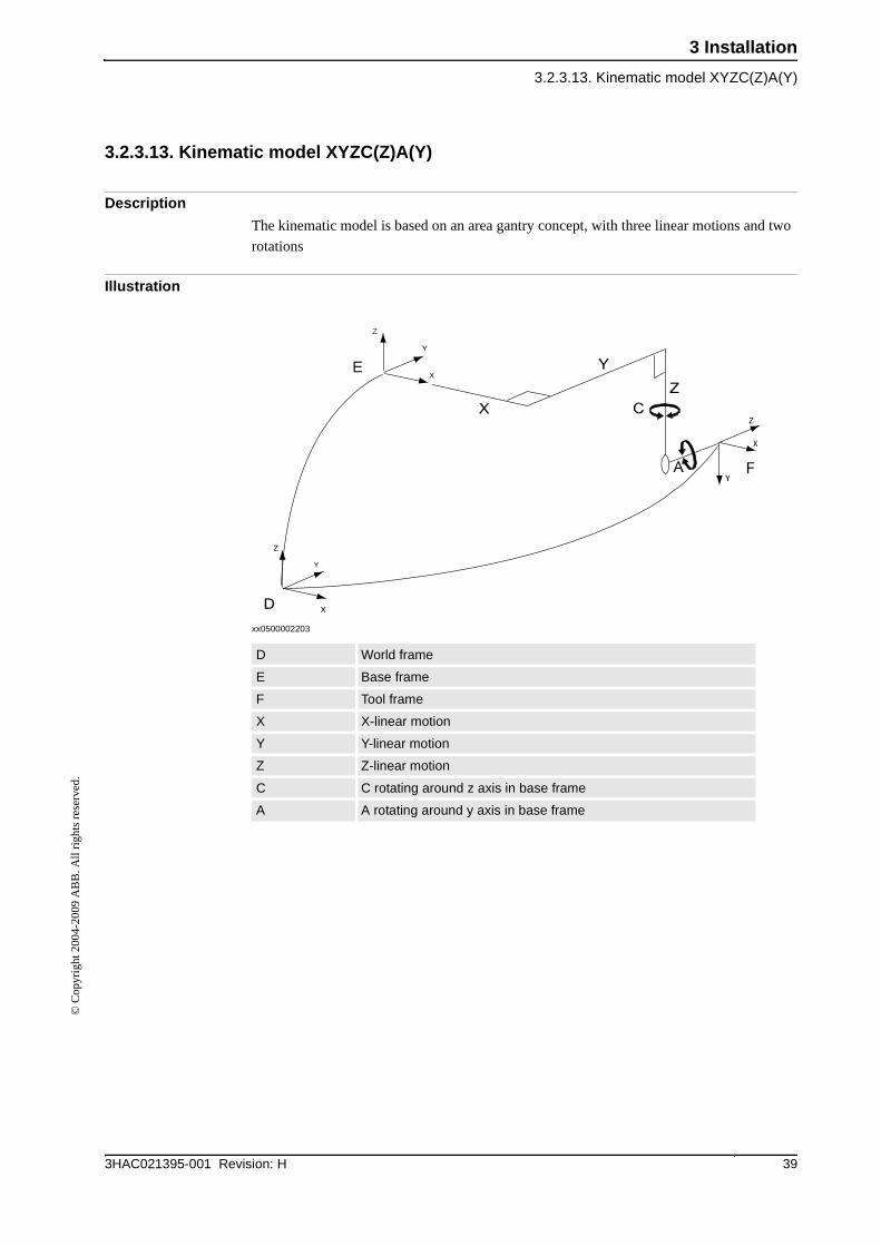
3.2.3.13. Kinematic model XYZC(Z)A(Y)
Description
The kinematic model is based on an area gantry concept, with three linear motions and two
rotations
Illustration
xx0500002203
D World frame
E Base frame
F Tool frame
X X-linear motion
Y Y-linear motion
Z Z-linear motion
C C rotating around z axis in base frame
A A rotating around y axis in base frame
3 Installation
3.2.3.14. Kinematic model XZ
3HAC021395-001 Revision: H40
© C
opyr
ight
200
4-20
09 A
BB
. All
righ
ts r
eser
ved.
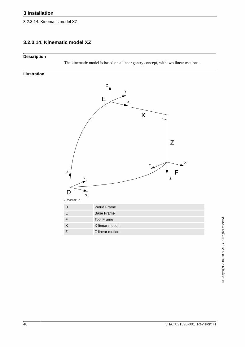
3.2.3.14. Kinematic model XZ
Description
The kinematic model is based on a linear gantry concept, with two linear motions.
Illustration
xx0500002110
D World Frame
E Base Frame
F Tool Frame
X X-linear motion
Z Z-linear motion
3 Installation
3.2.3.15. Kinematic model XZC(Z)
413HAC021395-001 Revision: H
© C
opyr
ight
200
4-20
09 A
BB
. All
righ
ts r
eser
ved.
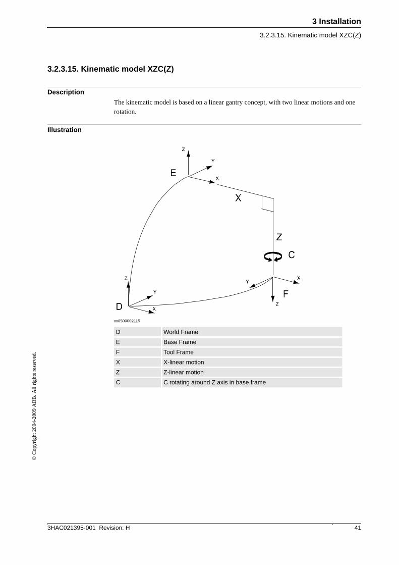
3.2.3.15. Kinematic model XZC(Z)
Description
The kinematic model is based on a linear gantry concept, with two linear motions and one
rotation.
Illustration
xx0500002115
D World Frame
E Base Frame
F Tool Frame
X X-linear motion
Z Z-linear motion
C C rotating around Z axis in base frame
3 Installation
3.2.3.16. Kinematic model XZB(X)
3HAC021395-001 Revision: H42
© C
opyr
ight
200
4-20
09 A
BB
. All
righ
ts r
eser
ved.
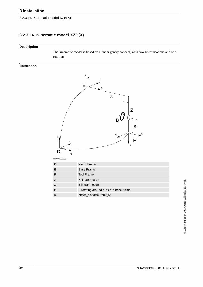
3.2.3.16. Kinematic model XZB(X)
Description
The kinematic model is based on a linear gantry concept, with two linear motions and one
rotation.
Illustration
xx0500002111
D World Frame
E Base Frame
F Tool Frame
X X-linear motion
Z Z-linear motion
B B rotating around X axis in base frame
a offset_z of arm “robx_6”
3 Installation
3.2.3.17. Kinematic model XZB(Y)
433HAC021395-001 Revision: H
© C
opyr
ight
200
4-20
09 A
BB
. All
righ
ts r
eser
ved.
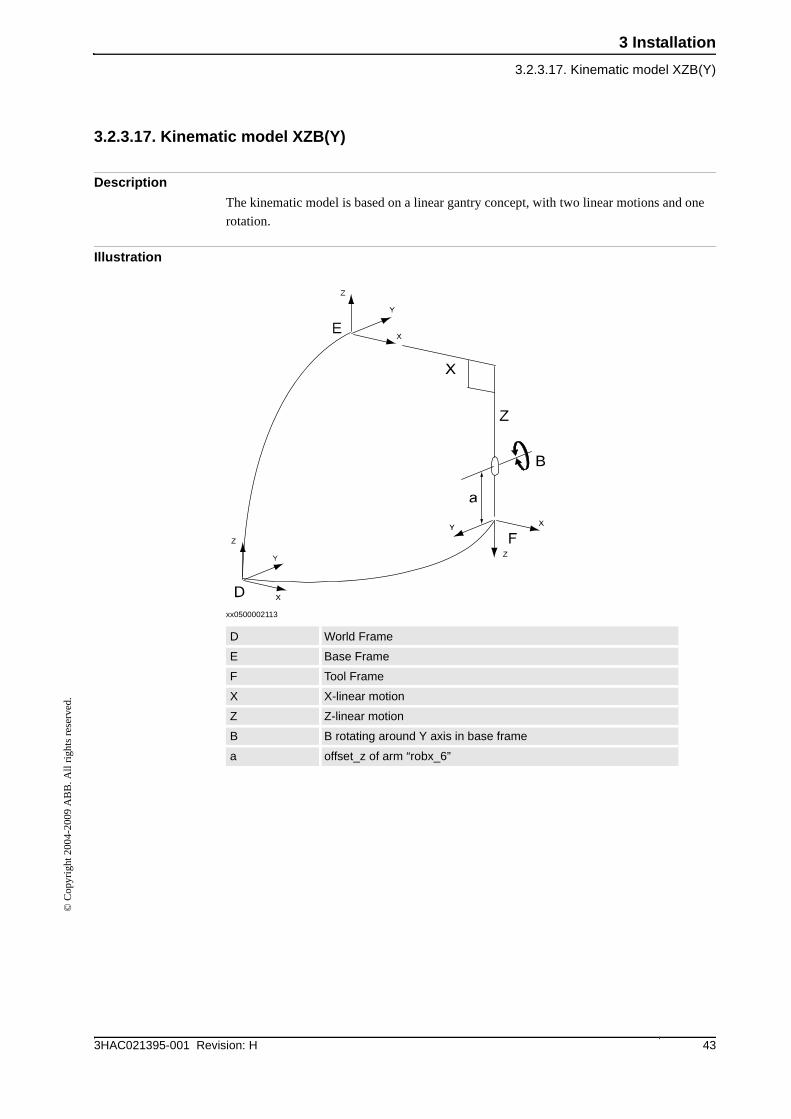
3.2.3.17. Kinematic model XZB(Y)
Description
The kinematic model is based on a linear gantry concept, with two linear motions and one
rotation.
Illustration
xx0500002113
D World Frame
E Base Frame
F Tool Frame
X X-linear motion
Z Z-linear motion
B B rotating around Y axis in base frame
a offset_z of arm “robx_6”
3 Installation
3.2.3.18. Kinematic model XZC(Z)B(X)
3HAC021395-001 Revision: H44
© C
opyr
ight
200
4-20
09 A
BB
. All
righ
ts r
eser
ved.
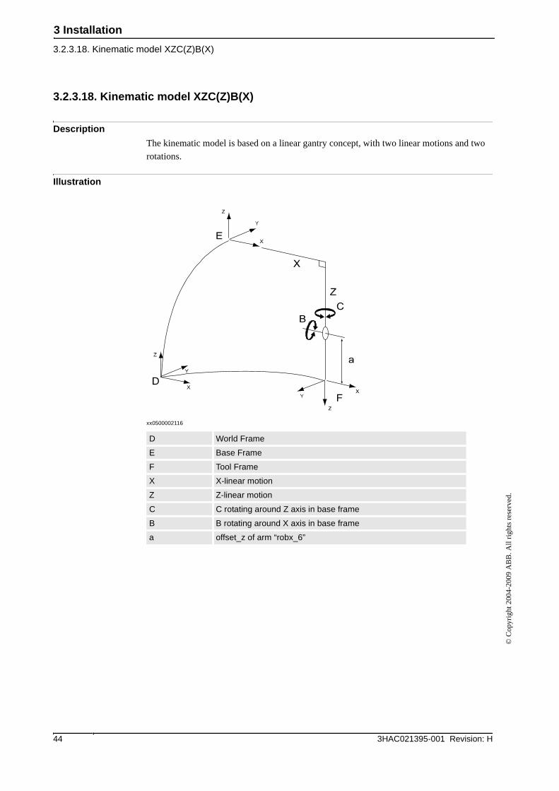
3.2.3.18. Kinematic model XZC(Z)B(X)
Description
The kinematic model is based on a linear gantry concept, with two linear motions and two
rotations.
Illustration
xx0500002116
D World Frame
E Base Frame
F Tool Frame
X X-linear motion
Z Z-linear motion
C C rotating around Z axis in base frame
B B rotating around X axis in base frame
a offset_z of arm “robx_6”
3 Installation
3.2.3.19. Kinematic model XZC(Z)B(Y)
453HAC021395-001 Revision: H
© C
opyr
ight
200
4-20
09 A
BB
. All
righ
ts r
eser
ved.
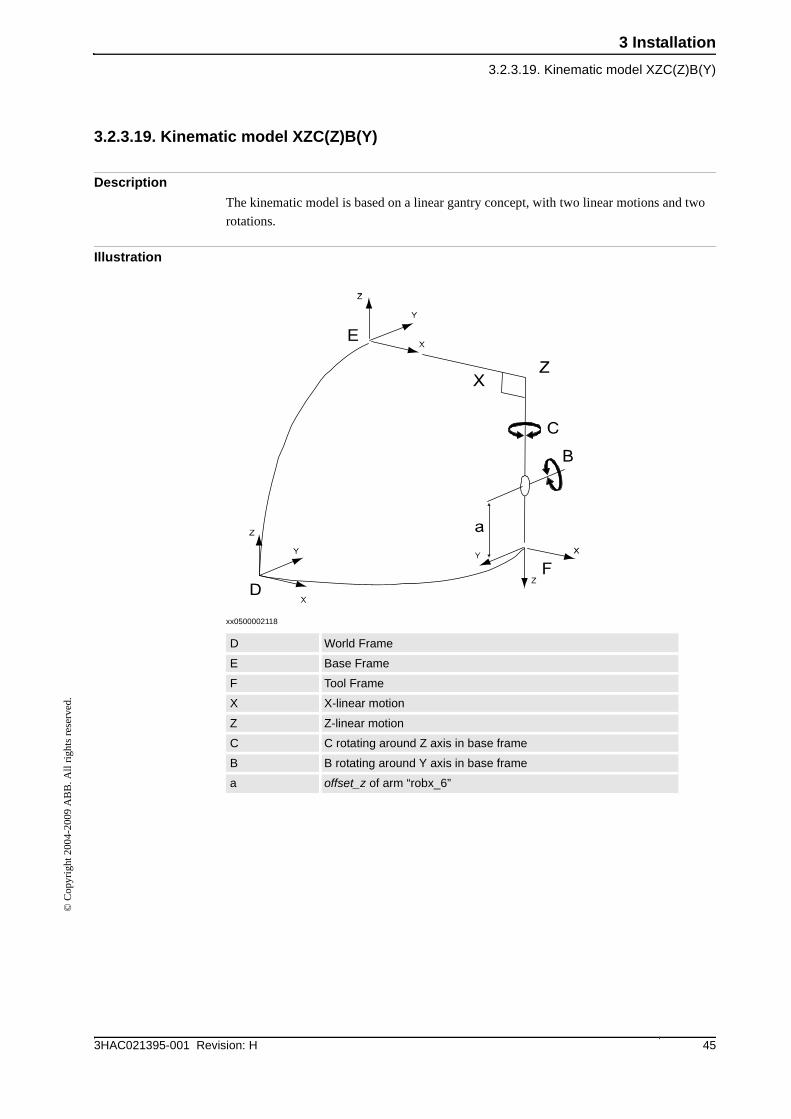
3.2.3.19. Kinematic model XZC(Z)B(Y)
Description
The kinematic model is based on a linear gantry concept, with two linear motions and two
rotations.
Illustration
xx0500002118
D World Frame
E Base Frame
F Tool Frame
X X-linear motion
Z Z-linear motion
C C rotating around Z axis in base frame
B B rotating around Y axis in base frame
a offset_z of arm “robx_6”
3 Installation
3.2.3.20. Kinematic model XZB(X)A(Z)
3HAC021395-001 Revision: H46
© C
opyr
ight
200
4-20
09 A
BB
. All
righ
ts r
eser
ved.
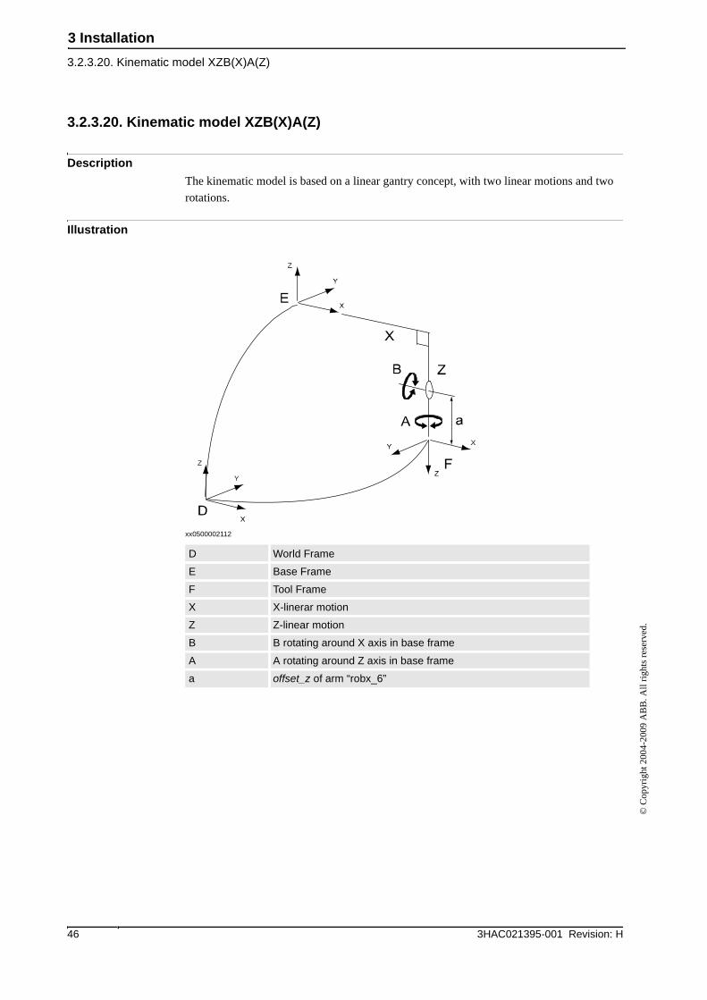
3.2.3.20. Kinematic model XZB(X)A(Z)
Description
The kinematic model is based on a linear gantry concept, with two linear motions and two
rotations.
Illustration
xx0500002112
D World Frame
E Base Frame
F Tool Frame
X X-linerar motion
Z Z-linear motion
B B rotating around X axis in base frame
A A rotating around Z axis in base frame
a offset_z of arm “robx_6”
3 Installation
3.2.3.21. Kinematic model XZB(Y)A(Z)
473HAC021395-001 Revision: H
© C
opyr
ight
200
4-20
09 A
BB
. All
righ
ts r
eser
ved.
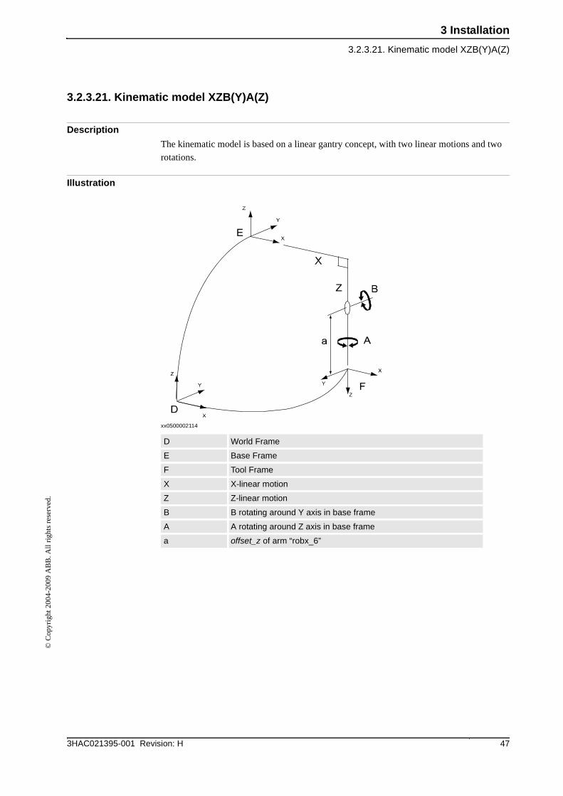
3.2.3.21. Kinematic model XZB(Y)A(Z)
Description
The kinematic model is based on a linear gantry concept, with two linear motions and two
rotations.
Illustration
xx0500002114
D World Frame
E Base Frame
F Tool Frame
X X-linear motion
Z Z-linear motion
B B rotating around Y axis in base frame
A A rotating around Z axis in base frame
a offset_z of arm “robx_6”
3 Installation
3.2.3.22. Kinematic model XZC(Z)B(X)A(Z)
3HAC021395-001 Revision: H48
© C
opyr
ight
200
4-20
09 A
BB
. All
righ
ts r
eser
ved.
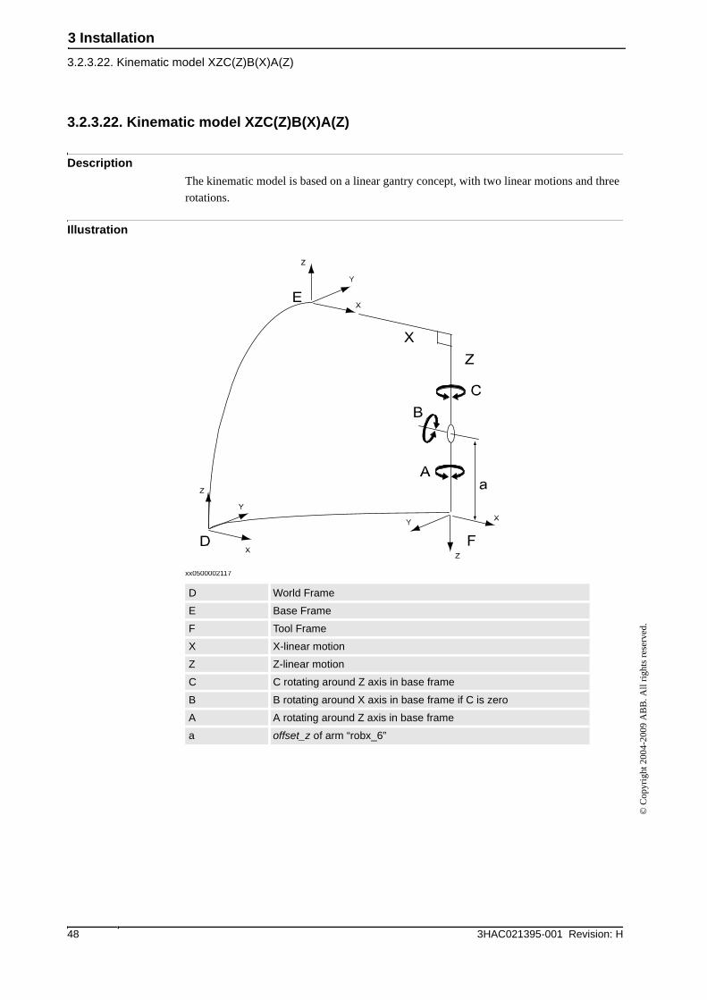
3.2.3.22. Kinematic model XZC(Z)B(X)A(Z)
Description
The kinematic model is based on a linear gantry concept, with two linear motions and three
rotations.
Illustration
xx0500002117
D World Frame
E Base Frame
F Tool Frame
X X-linear motion
Z Z-linear motion
C C rotating around Z axis in base frame
B B rotating around X axis in base frame if C is zero
A A rotating around Z axis in base frame
a offset_z of arm “robx_6”
3 Installation
3.2.3.23. Kinematic model YZ
493HAC021395-001 Revision: H
© C
opyr
ight
200
4-20
09 A
BB
. All
righ
ts r
eser
ved.
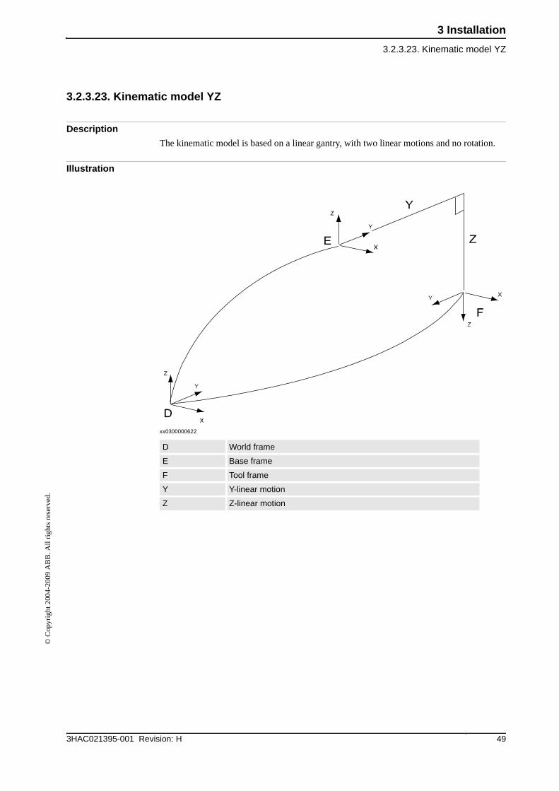
3.2.3.23. Kinematic model YZ
Description
The kinematic model is based on a linear gantry, with two linear motions and no rotation.
Illustration
xx0300000622
D World frame
E Base frame
F Tool frame
Y Y-linear motion
Z Z-linear motion
3 Installation
3.2.3.24. Kinematic model YZC(Z)
3HAC021395-001 Revision: H50
© C
opyr
ight
200
4-20
09 A
BB
. All
righ
ts r
eser
ved.
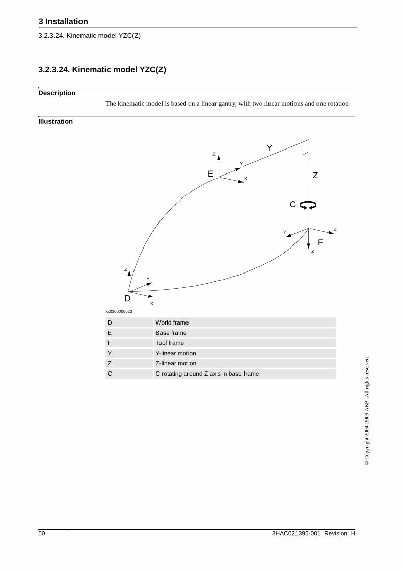
3.2.3.24. Kinematic model YZC(Z)
Description
The kinematic model is based on a linear gantry, with two linear motions and one rotation.
Illustration
xx0300000623
D World frame
E Base frame
F Tool frame
Y Y-linear motion
Z Z-linear motion
C C rotating around Z axis in base frame
3 Installation
3.2.3.25. Kinematic model YZB(X)
513HAC021395-001 Revision: H
© C
opyr
ight
200
4-20
09 A
BB
. All
righ
ts r
eser
ved.
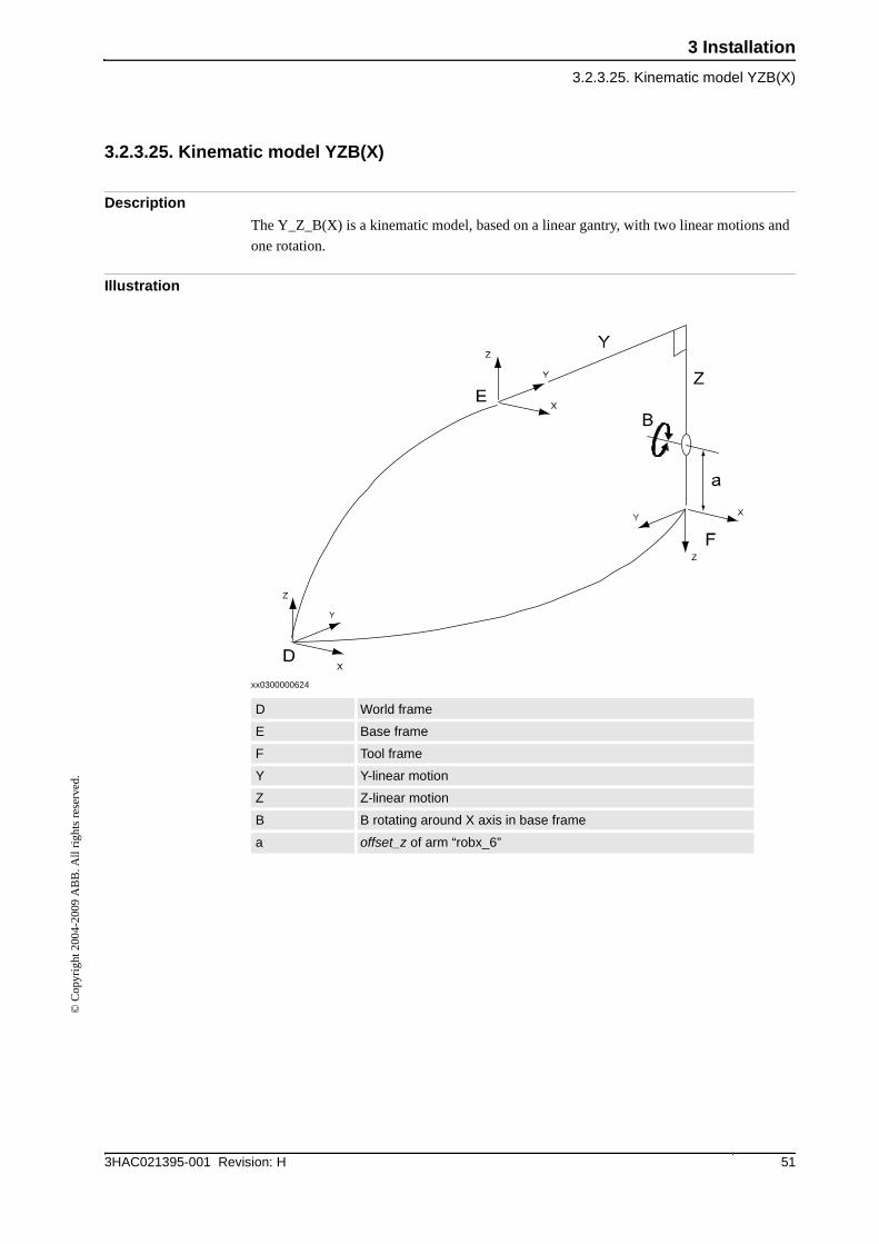
3.2.3.25. Kinematic model YZB(X)
Description
The Y_Z_B(X) is a kinematic model, based on a linear gantry, with two linear motions and
one rotation.
Illustration
xx0300000624
D World frame
E Base frame
F Tool frame
Y Y-linear motion
Z Z-linear motion
B B rotating around X axis in base frame
a offset_z of arm “robx_6”
3 Installation
3.2.3.26. Kinematic model YZB(Y)
3HAC021395-001 Revision: H52
© C
opyr
ight
200
4-20
09 A
BB
. All
righ
ts r
eser
ved.
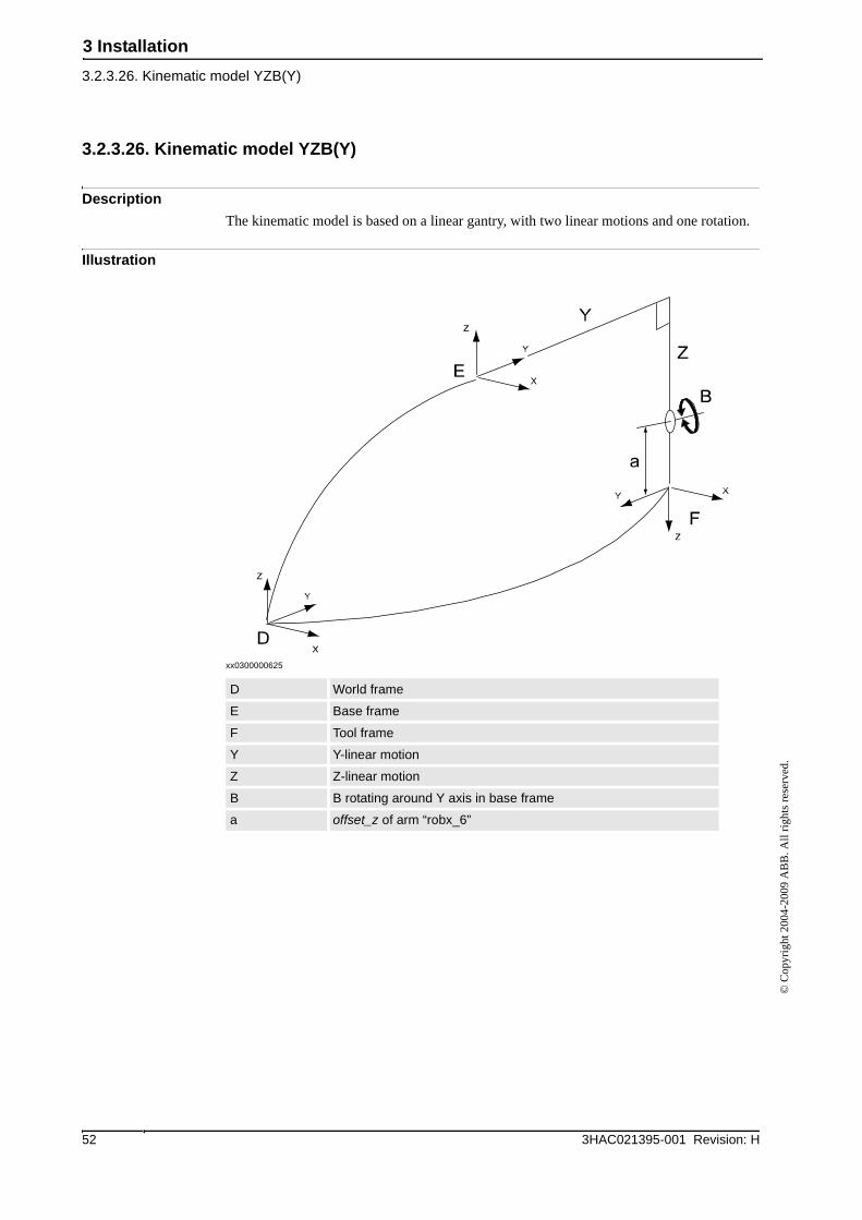
3.2.3.26. Kinematic model YZB(Y)
Description
The kinematic model is based on a linear gantry, with two linear motions and one rotation.
Illustration
xx0300000625
D World frame
E Base frame
F Tool frame
Y Y-linear motion
Z Z-linear motion
B B rotating around Y axis in base frame
a offset_z of arm “robx_6”

3 Installation
3.2.3.27. Kinematic model YZC(Z)B(X)
533HAC021395-001 Revision: H
© C
opyr
ight
200
4-20
09 A
BB
. All
righ
ts r
eser
ved.
3.2.3.27. Kinematic model YZC(Z)B(X)
Description
The kinematic model is based on a linear gantry concept, with two linear motions and two
rotations.
Illustration
xx0500002119
D World Frame
E Base Frame
F Tool Frame
Y Y-linear motion
Z Z-linear motion
C C rotating around Z axis in base frame
B B rotating around X axis in base frame if C is zero
a offset_z of arm “robx_6”
3 Installation
3.2.3.28. Kinematic model YZC(Z)B(Y)
3HAC021395-001 Revision: H54
© C
opyr
ight
200
4-20
09 A
BB
. All
righ
ts r
eser
ved.
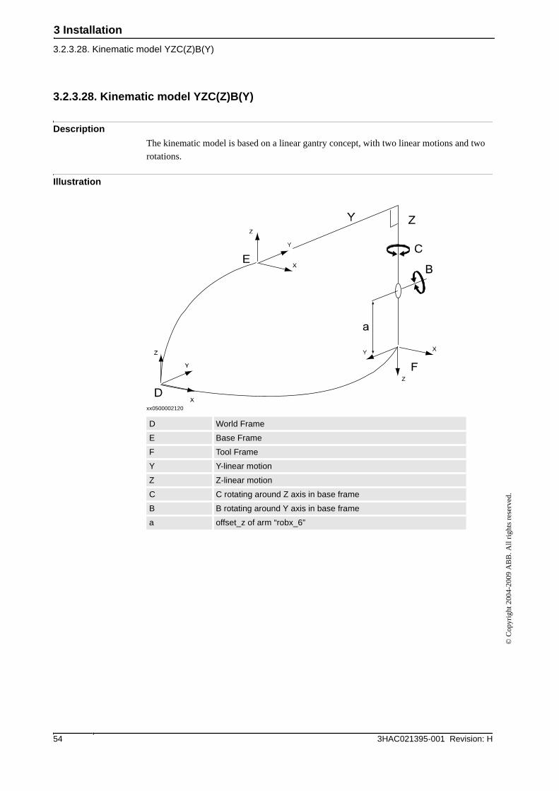
3.2.3.28. Kinematic model YZC(Z)B(Y)
Description
The kinematic model is based on a linear gantry concept, with two linear motions and two
rotations.
Illustration
xx0500002120
D World Frame
E Base Frame
F Tool Frame
Y Y-linear motion
Z Z-linear motion
C C rotating around Z axis in base frame
B B rotating around Y axis in base frame
a offset_z of arm “robx_6”
3 Installation
3.2.3.29. Kinematic model YZB(X)A(Z)
553HAC021395-001 Revision: H
© C
opyr
ight
200
4-20
09 A
BB
. All
righ
ts r
eser
ved.
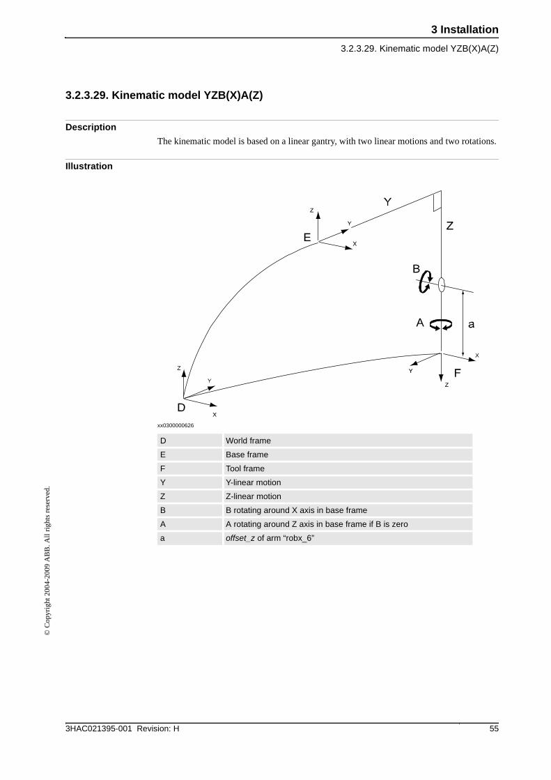
3.2.3.29. Kinematic model YZB(X)A(Z)
Description
The kinematic model is based on a linear gantry, with two linear motions and two rotations.
Illustration
xx0300000626
D World frame
E Base frame
F Tool frame
Y Y-linear motion
Z Z-linear motion
B B rotating around X axis in base frame
A A rotating around Z axis in base frame if B is zero
a offset_z of arm “robx_6”
3 Installation
3.2.3.30. Kinematic model YZB(Y)A(Z)
3HAC021395-001 Revision: H56
© C
opyr
ight
200
4-20
09 A
BB
. All
righ
ts r
eser
ved.
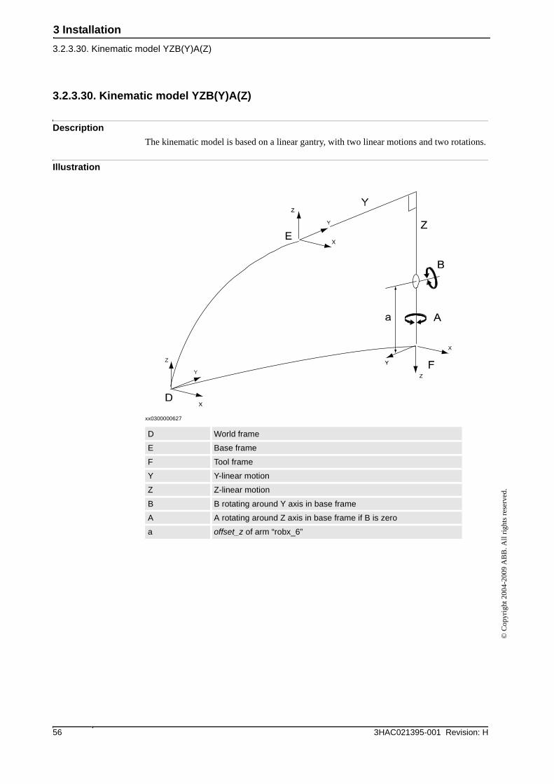
3.2.3.30. Kinematic model YZB(Y)A(Z)
Description
The kinematic model is based on a linear gantry, with two linear motions and two rotations.
Illustration
xx0300000627
D World frame
E Base frame
F Tool frame
Y Y-linear motion
Z Z-linear motion
B B rotating around Y axis in base frame
A A rotating around Z axis in base frame if B is zero
a offset_z of arm “robx_6”
3 Installation
3.2.3.31. Kinematic modelYZC(Z)B(X)A(Z)
573HAC021395-001 Revision: H
© C
opyr
ight
200
4-20
09 A
BB
. All
righ
ts r
eser
ved.
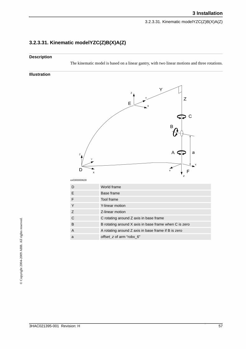
3.2.3.31. Kinematic modelYZC(Z)B(X)A(Z)
Description
The kinematic model is based on a linear gantry, with two linear motions and three rotations.
Illustration
xx0300000628
D World frame
E Base frame
F Tool frame
Y Y-linear motion
Z Z-linear motion
C C rotating around Z axis in base frame
B B rotating around X axis in base frame when C is zero
A A rotating around Z axis in base frame if B is zero
a offset_z of arm “robx_6”
3 Installation
3.2.3.32. Kinematic model YZC(Z)B(Y)A(Z)
3HAC021395-001 Revision: H58
© C
opyr
ight
200
4-20
09 A
BB
. All
righ
ts r
eser
ved.
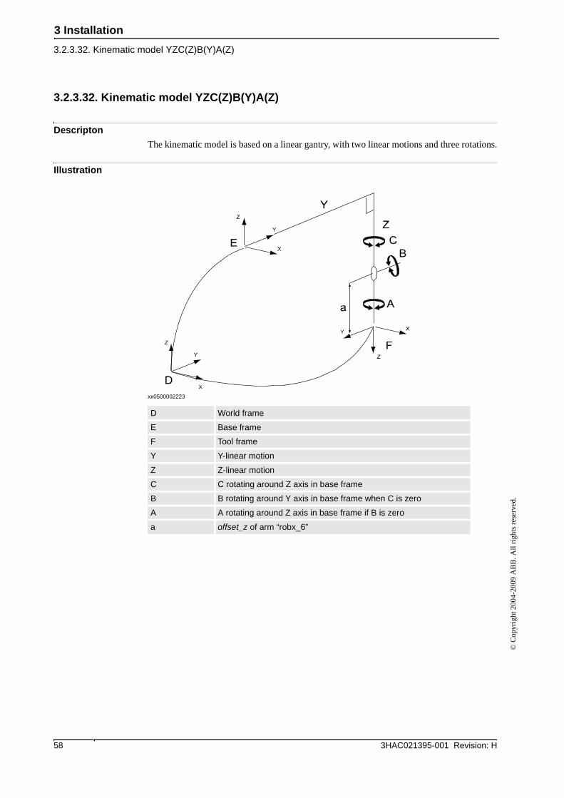
3.2.3.32. Kinematic model YZC(Z)B(Y)A(Z)
Descripton
The kinematic model is based on a linear gantry, with two linear motions and three rotations.
Illustration
xx0500002223
D World frame
E Base frame
F Tool frame
Y Y-linear motion
Z Z-linear motion
C C rotating around Z axis in base frame
B B rotating around Y axis in base frame when C is zero
A A rotating around Z axis in base frame if B is zero
a offset_z of arm “robx_6”
3 Installation
3.2.3.33. Kinematic model YE(Y)D(Y)B(Y)A(Z)
593HAC021395-001 Revision: H
© C
opyr
ight
200
4-20
09 A
BB
. All
righ
ts r
eser
ved.
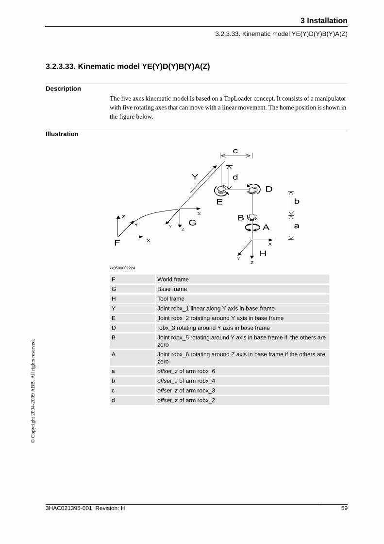
3.2.3.33. Kinematic model YE(Y)D(Y)B(Y)A(Z)
Description
The five axes kinematic model is based on a TopLoader concept. It consists of a manipulator
with five rotating axes that can move with a linear movement. The home position is shown in
the figure below.
Illustration
xx0500002224
F World frame
G Base frame
H Tool frame
Y Joint robx_1 linear along Y axis in base frame
E Joint robx_2 rotating around Y axis in base frame
D robx_3 rotating around Y axis in base frame
B Joint robx_5 rotating around Y axis in base frame if the others are zero
A Joint robx_6 rotating around Z axis in base frame if the others are zero
a offset_z of arm robx_6
b offset_z of arm robx_4
c offset_z of arm robx_3
d offset_z of arm robx_2
3 Installation
3.2.3.34. Kinematic model YE(Y)D(Y)C(Z)B(Y)A(Z)
3HAC021395-001 Revision: H60
© C
opyr
ight
200
4-20
09 A
BB
. All
righ
ts r
eser
ved.
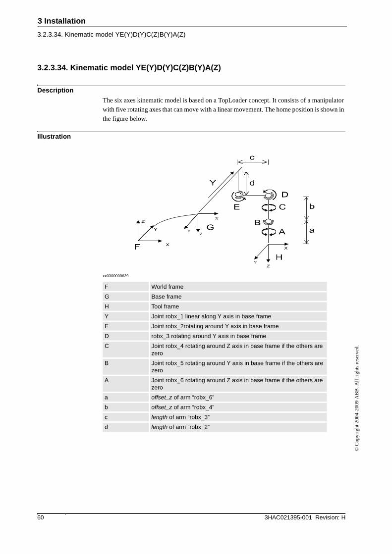
3.2.3.34. Kinematic model YE(Y)D(Y)C(Z)B(Y)A(Z)
Description
The six axes kinematic model is based on a TopLoader concept. It consists of a manipulator
with five rotating axes that can move with a linear movement. The home position is shown in
the figure below.
Illustration
xx0300000629
F World frame
G Base frame
H Tool frame
Y Joint robx_1 linear along Y axis in base frame
E Joint robx_2rotating around Y axis in base frame
D robx_3 rotating around Y axis in base frame
C Joint robx_4 rotating around Z axis in base frame if the others are zero
B Joint robx_5 rotating around Y axis in base frame if the others are zero
A Joint robx_6 rotating around Z axis in base frame if the others are zero
a offset_z of arm “robx_6”
b offset_z of arm “robx_4”
c length of arm “robx_3”
d length of arm “robx_2”
3 Installation
3.2.3.35. Doppin Feeder
613HAC021395-001 Revision: H
© C
opyr
ight
200
4-20
09 A
BB
. All
righ
ts r
eser
ved.
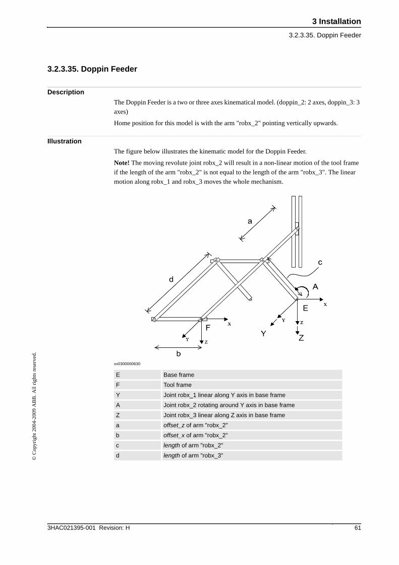
3.2.3.35. Doppin Feeder
Description
The Doppin Feeder is a two or three axes kinematical model. (doppin_2: 2 axes, doppin_3: 3
axes)
Home position for this model is with the arm "robx_2" pointing vertically upwards.
Illustration
The figure below illustrates the kinematic model for the Doppin Feeder.
Note! The moving revolute joint robx_2 will result in a non-linear motion of the tool frame
if the length of the arm "robx_2" is not equal to the length of the arm "robx_3". The linear
motion along robx_1 and robx_3 moves the whole mechanism.
xx0300000630
E Base frame
F Tool frame
Y Joint robx_1 linear along Y axis in base frame
A Joint robx_2 rotating around Y axis in base frame
Z Joint robx_3 linear along Z axis in base frame
a offset_z of arm "robx_2"
b offset_x of arm "robx_2"
c length of arm "robx_2"
d length of arm "robx_3"
3 Installation
3.2.4. Creating a stand alone controller system
3HAC021395-001 Revision: H62
© C
opyr
ight
200
4-20
09 A
BB
. All
righ
ts r
eser
ved.
3.2.4. Creating a stand alone controller system
Overview
This section describes how to create a stand alone controller system. To do this you use the
robot’s software CD and the System Builder in RobotStudio.
General procedure
Follow these basic steps to create a stand alone controller system. For more information on
how to install RobotWare, create a new system and add additional options see Operating
manual - RobotStudio.
System Builder procedure
General information about creating a new system is available in the Help menu in
RobotStudio. This section gives information specific for the stand alone controller option.
Action
1. Install RobotWare from the robot’s software CD to your PC, as described in Operating manual - RobotStudio.
2. Run setup.exe located in the folder Additional Options/StandAloneController on the CD.
3. Create a stand alone controller system using the System Builder in RobotStudio. How to do this is detailed in System Builder procedure on page 62.
4. Download the system to the robot controller by using System Builder. See Installation of system to robot controller on page 64.
Action
1. In RobotStudio, open System Builder and click the Create New button.
2. In one of the dialogs a key for the additional option should be entered. Browse to Mediapool/SAC_5.XX.XXXX on your PC, where the option key file is located. Select the key file (.kxt) and click Open.
Continues on next page
3 Installation
3.2.4. Creating a stand alone controller system
633HAC021395-001 Revision: H
© C
opyr
ight
200
4-20
09 A
BB
. All
righ
ts r
eser
ved.
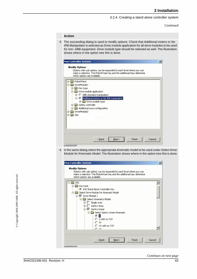
3. The succeeding dialog is used to modify options. Check that Additional motors or No IRB Manipulator is selected as Drive module application for all drive modules to be used for non- ABB equipment. Drive module type should be selected as well. The illustration shows where in the option tree this is done.
en0600002987
4. In the same dialog select the appropriate kinematic model to be used under Select Drive Module for Kinematic Model. The illustration shows where in the option tree this is done.
en0500002433
Action
Continued
Continues on next page
3 Installation
3.2.4. Creating a stand alone controller system
3HAC021395-001 Revision: H64
© C
opyr
ight
200
4-20
09 A
BB
. All
righ
ts r
eser
ved.
Installation of system to robot controller
Download the system to the robot controller by using System Builder in RobotStudio.
Information on how to do this is available in the Help menu. At the end of the installation
process you are asked if you want the controller to restart. Confirm and wait until the system
has started up.
Errors at start up
When the system is ready with start-up inform yourself on system status by studying the event
log on the FlexPendant or in RobotStudio. A system with non-ABB equipment needs
configuration to become functional, and it is even quite likely that your system is in system
failure state at this point. Ignore any errors until you are ready with the configuration
procedure described in section Minimal configuration of non-ABB robots on page 76. If there
are remaining errors after configuration is done find out more about error localization in
section Error management on page 145.
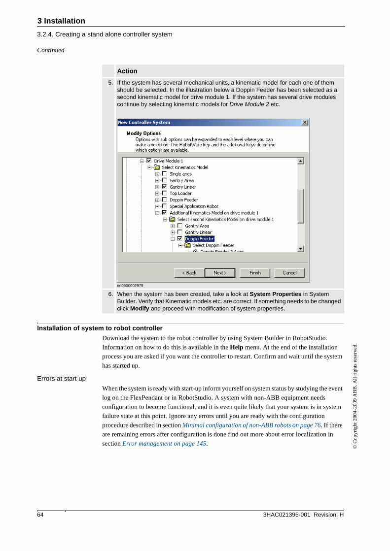
5. If the system has several mechanical units, a kinematic model for each one of them should be selected. In the illustration below a Doppin Feeder has been selected as a second kinematic model for drive module 1. If the system has several drive modules continue by selecting kinematic models for Drive Module 2 etc.
en0600002979
6. When the system has been created, take a look at System Properties in System Builder. Verify that Kinematic models etc. are correct. If something needs to be changed click Modify and proceed with modification of system properties.
Action
Continued
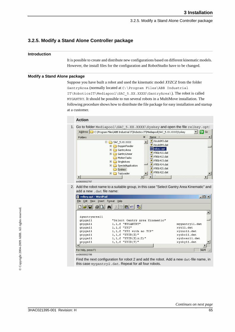
3 Installation
3.2.5. Modify a Stand Alone Controller package
653HAC021395-001 Revision: H
© C
opyr
ight
200
4-20
09 A
BB
. All
righ
ts r
eser
ved.
3.2.5. Modify a Stand Alone Controller package
Introduction
It is possible to create and distribute new configurations based on different kinematic models.
However, the install files for the configuration and RobotStudio have to be changed.
Modify a Stand Alone package
Suppose you have built a robot and used the kinematic model XYZCZ from the folder
GantryArea (normally located at C:\Program Files\ABB Industrial
IT\RoboticsIT\Mediapool\SAC_5.XX.XXXX\GantryArea\). The robot is called
MYGANTRY. It should be possible to run several robots in a MultiMove installation. The
following procedure shows how to distribute the file package for easy installation and startup
at a customer.
Action
1. Go to folder Mediapool\SAC_5.XX.XXXX\Syskey and open the file relkey.opt:
en0600002797
2. Add the robot name to a suitable group, in this case "Select Gantry Area Kinematic" and add a new .dat file name:
en0600002798
Find the next configuration for robot 2 and add the robot. Add a new dat-file name, in this case mygantry2.dat. Repeat for all four robots.
Continues on next page
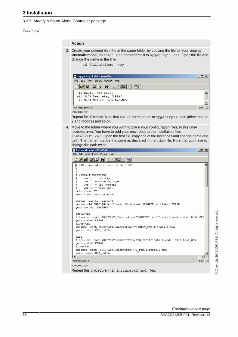
3 Installation
3.2.5. Modify a Stand Alone Controller package
3HAC021395-001 Revision: H66
© C
opyr
ight
200
4-20
09 A
BB
. All
righ
ts r
eser
ved.
3. Create your defined dat-file in the same folder by copying the file for your original kinematic model, xyzcz11.dat and rename it to mygantry11.dat. Open the file and change the name in the line:
-id SAC11Select -key
en0600002799
Repeat for all robots. Note that SAC21 corresponds to mygantry21.dat (drive module 2 and robot 1) and so on.
4. Move to the folder where you want to place your configuration files, in this case GantryArea. You have to add your new robot to the installation files instareaX1.cmd. Open the first file, copy one of the instances and change name and path. The name must be the same as declared in the .dat-file. Note that you have to change the path twice:
en0600002800
Repeat this procedure in all instareaXX.cmd files.
Action
Continued
Continues on next page
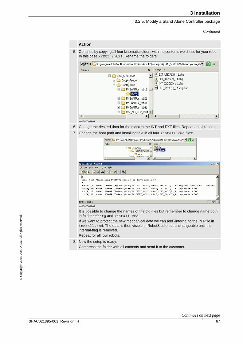
3 Installation
3.2.5. Modify a Stand Alone Controller package
673HAC021395-001 Revision: H
© C
opyr
ight
200
4-20
09 A
BB
. All
righ
ts r
eser
ved.
5. Continue by copying all four kinematic folders with the contents we chose for your robot. In this case XYZCZ_robX1. Rename the folders:
en0600002801
6. Change the desired data for the robot in the INT and EXT files. Repeat on all robots.
7. Change the boot path and installing text in all four install.cmd files:
en0600002802
It is possible to change the names of the cfg-files but remember to change name both in folder irbcfg and install.cmd.
If we want to protect the new mechanical data we can add -internal to the INT-file in install.cmd. The data is then visible in RobotStudio but unchangeable until the -internal-flag is removed.
Repeat for all four robots.
8. Now the setup is ready.
Compress the folder with all contents and send it to the customer.
Action
Continued
Continues on next page
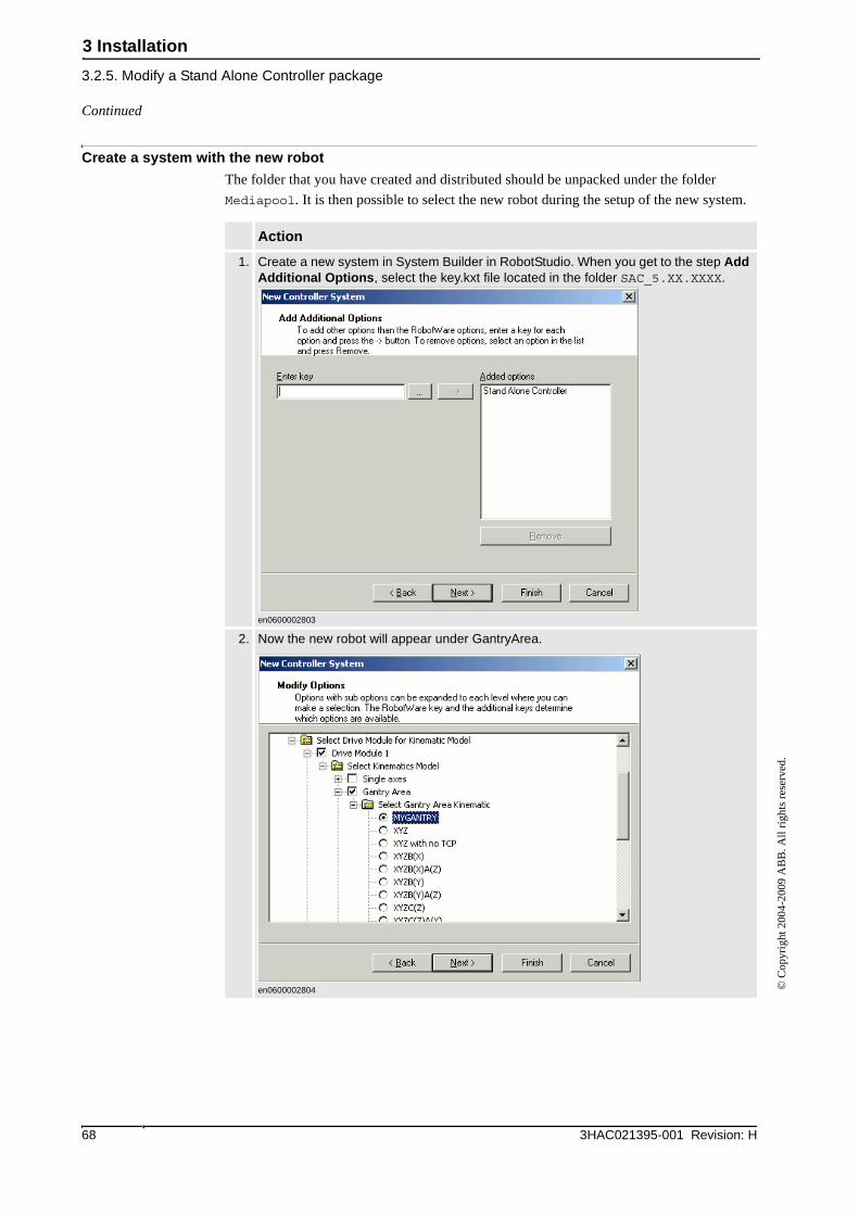
3 Installation
3.2.5. Modify a Stand Alone Controller package
3HAC021395-001 Revision: H68
© C
opyr
ight
200
4-20
09 A
BB
. All
righ
ts r
eser
ved.
Create a system with the new robot
The folder that you have created and distributed should be unpacked under the folder
Mediapool. It is then possible to select the new robot during the setup of the new system.
Action
1. Create a new system in System Builder in RobotStudio. When you get to the step Add Additional Options, select the key.kxt file located in the folder SAC_5.XX.XXXX.
en0600002803
2. Now the new robot will appear under GantryArea.
en0600002804
Continued
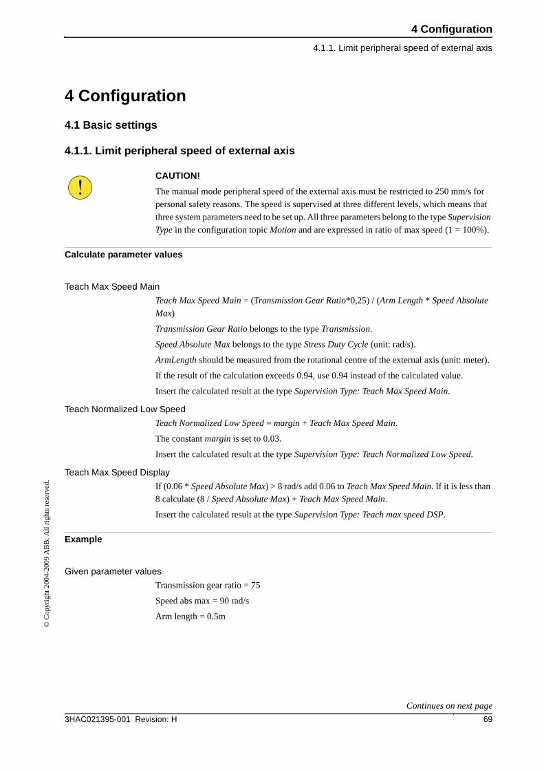
4 Configuration
4.1.1. Limit peripheral speed of external axis
693HAC021395-001 Revision: H
© C
opyr
ight
200
4-20
09 A
BB
. All
righ
ts r
eser
ved.
4 Configuration
4.1 Basic settings
4.1.1. Limit peripheral speed of external axis
CAUTION!
The manual mode peripheral speed of the external axis must be restricted to 250 mm/s for
personal safety reasons. The speed is supervised at three different levels, which means that
three system parameters need to be set up. All three parameters belong to the type Supervision
Type in the configuration topic Motion and are expressed in ratio of max speed (1 = 100%).
Calculate parameter values
Teach Max Speed Main
Teach Max Speed Main = (Transmission Gear Ratio*0,25) / (Arm Length * Speed Absolute
Max)
Transmission Gear Ratio belongs to the type Transmission.
Speed Absolute Max belongs to the type Stress Duty Cycle (unit: rad/s).
ArmLength should be measured from the rotational centre of the external axis (unit: meter).
If the result of the calculation exceeds 0.94, use 0.94 instead of the calculated value.
Insert the calculated result at the type Supervision Type: Teach Max Speed Main.
Teach Normalized Low Speed
Teach Normalized Low Speed = margin + Teach Max Speed Main.
The constant margin is set to 0.03.
Insert the calculated result at the type Supervision Type: Teach Normalized Low Speed.
Teach Max Speed Display
If (0.06 * Speed Absolute Max) > 8 rad/s add 0.06 to Teach Max Speed Main. If it is less than
8 calculate (8 / Speed Absolute Max) + Teach Max Speed Main.
Insert the calculated result at the type Supervision Type: Teach max speed DSP.
Example
Given parameter values
Transmission gear ratio = 75
Speed abs max = 90 rad/s
Arm length = 0.5m
Continues on next page
4 Configuration
4.1.1. Limit peripheral speed of external axis
3HAC021395-001 Revision: H70
© C
opyr
ight
200
4-20
09 A
BB
. All
righ
ts r
eser
ved.
Calculations
Teach Max Speed Main = (75 * 0.25) / (0.5 * 90) = 0.417
Teach Normalized Low Speed = 0.417 + 0.03 = 0.447
0.06 * Speed Absolute Max = 0.06 * 90 = 5.4
As 5.4 is less than 8 we add the following to the result
Teach Max Speed Dsp = 0.417 + (8 / 90) = 0.506
Continued
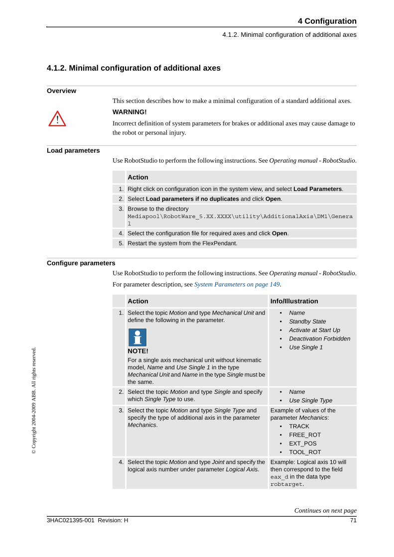
4 Configuration
4.1.2. Minimal configuration of additional axes
713HAC021395-001 Revision: H
© C
opyr
ight
200
4-20
09 A
BB
. All
righ
ts r
eser
ved.
4.1.2. Minimal configuration of additional axes
Overview
This section describes how to make a minimal configuration of a standard additional axes.
WARNING!
Incorrect definition of system parameters for brakes or additional axes may cause damage to
the robot or personal injury.
Load parameters
Use RobotStudio to perform the following instructions. See Operating manual - RobotStudio.
Configure parameters
Use RobotStudio to perform the following instructions. See Operating manual - RobotStudio.
For parameter description, see System Parameters on page 149.
Action
1. Right click on configuration icon in the system view, and select Load Parameters.
2. Select Load parameters if no duplicates and click Open.
3. Browse to the directory Mediapool\RobotWare_5.XX.XXXX\utility\AdditionalAxis\DM1\General
4. Select the configuration file for required axes and click Open.
5. Restart the system from the FlexPendant.
Action Info/Illustration
1. Select the topic Motion and type Mechanical Unit and define the following in the parameter.
NOTE!For a single axis mechanical unit without kinematic model, Name and Use Single 1 in the type Mechanical Unit and Name in the type Single must be the same.
• Name
• Standby State
• Activate at Start Up
• Deactivation Forbidden
• Use Single 1
2. Select the topic Motion and type Single and specify which Single Type to use.
• Name
• Use Single Type
3. Select the topic Motion and type Single Type and specify the type of additional axis in the parameter Mechanics.
Example of values of the parameter Mechanics:
• TRACK
• FREE_ROT
• EXT_POS
• TOOL_ROT
4. Select the topic Motion and type Joint and specify the logical axis number under parameter Logical Axis.
Example: Logical axis 10 will then correspond to the field eax_d in the data type robtarget.
Continues on next page
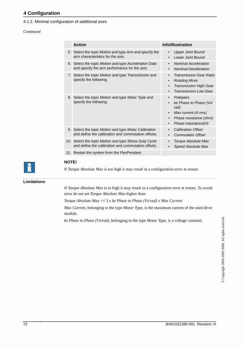
4 Configuration
4.1.2. Minimal configuration of additional axes
3HAC021395-001 Revision: H72
© C
opyr
ight
200
4-20
09 A
BB
. All
righ
ts r
eser
ved.
NOTE!
If Torque Absolute Max is too high it may result in a configuration error at restart.
Limitations
If Torque Absolute Max is to high it may result in a configuration error at restart. To avoid
error do not set Torque Absolute Max higher than:
Torque Absolute Max <√ 3 x ke Phase to Phase (Vs/rad) x Max Current
Max Current, belonging to the type Motor Type, is the maximum current of the used drive
module.
ke Phase to Phase (Vs/rad), belonging to the type Motor Type, is a voltage constant.
5. Select the topic Motion and type Arm and specify the arm characteristics for the axis.
• Upper Joint Bound
• Lower Joint Bound
6. Select the topic Motion and type Acceleration Data and specify the arm performance for the axis.
• Nominal Acceleration
• Nominal Deceleration
7. Select the topic Motion and type Transmission and specify the following.
• Transmission Gear Ratio
• Rotating Move
• Transmission High Gear
• Transmission Low Gear
8. Select the topic Motion and type Motor Type and specify the following.
• Polepairs
• ke Phase to Phase (Vs/rad)
• Max current (A rms)
• Phase resistance (ohm)
• Phase inductance(H)
9. Select the topic Motion and type Motor Calibration and define the calibration and commutation offsets.
• Calibration Offset
• Commutator Offset
10. Select the topic Motion and type Stress Duty Cycle and define the calibration and commutation offsets.
• Torque Absolute Max
• Speed Absolute Max
11. Restart the system from the FlexPendant.
Action Info/Illustration
Continued
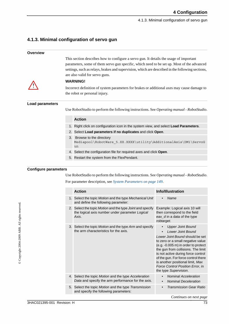
4 Configuration
4.1.3. Minimal configuration of servo gun
733HAC021395-001 Revision: H
© C
opyr
ight
200
4-20
09 A
BB
. All
righ
ts r
eser
ved.
4.1.3. Minimal configuration of servo gun
Overview
This section describes how to configure a servo gun. It details the usage of important
parameters, some of them servo gun specific, which need to be set up. Most of the advanced
settings, such as relays, brakes and supervision, which are described in the following sections,
are also valid for servo guns.
WARNING!
Incorrect definition of system parameters for brakes or additional axes may cause damage to
the robot or personal injury.
Load parameters
Use RobotStudio to perform the following instructions. See Operating manual - RobotStudio.
Configure parameters
Use RobotStudio to perform the following instructions. See Operating manual - RobotStudio.
For parameter description, see System Parameters on page 149.
Action
1. Right click on configuration icon in the system view, and select Load Parameters.
2. Select Load parameters if no duplicates and click Open.
3. Browse to the directory Mediapool\RobotWare_5.XX.XXXX\utility\AdditionalAxis\DM1\ServoGun
4. Select the configuration file for required axes and click Open.
5. Restart the system from the FlexPendant.
Action Info/Illustration
1. Select the topic Motion and the type Mechanical Unit and define the following parameter:
• Name
2. Select the topic Motion and the type Joint and specify the logical axis number under parameter Logical Axis.
Example: Logical axis 10 will then correspond to the field eax_d in a data of the type robtarget.
3. Select the topic Motion and the type Arm and specify the arm characteristics for the axis.
• Upper Joint Bound
• Lower Joint Bound
Lower Joint Bound should be set to zero or a small negative value (e.g. -0.005 m) in order to protect the gun from collisions. The limit is not active during force control of the gun. For force control there is another positional limit, Max Force Control Position Error, in the type Supervision.
4. Select the topic Motion and the type Acceleration Data and specify the arm performance for the axis.
• Nominal Acceleration
• Nominal Deceleration
5. Select the topic Motion and the type Transmission and specify the following parameters:
• Transmission Gear Ratio
Continues on next page
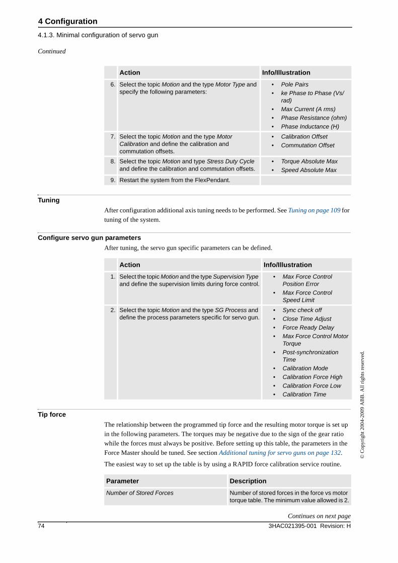
4 Configuration
4.1.3. Minimal configuration of servo gun
3HAC021395-001 Revision: H74
© C
opyr
ight
200
4-20
09 A
BB
. All
righ
ts r
eser
ved.
Tuning
After configuration additional axis tuning needs to be performed. See Tuning on page 109 for
tuning of the system.
Configure servo gun parameters
After tuning, the servo gun specific parameters can be defined.
Tip force
The relationship between the programmed tip force and the resulting motor torque is set up
in the following parameters. The torques may be negative due to the sign of the gear ratio
while the forces must always be positive. Before setting up this table, the parameters in the
Force Master should be tuned. See section Additional tuning for servo guns on page 132.
The easiest way to set up the table is by using a RAPID force calibration service routine.
6. Select the topic Motion and the type Motor Type and specify the following parameters:
• Pole Pairs
• ke Phase to Phase (Vs/rad)
• Max Current (A rms)
• Phase Resistance (ohm)
• Phase Inductance (H)
7. Select the topic Motion and the type Motor Calibration and define the calibration and commutation offsets.
• Calibration Offset
• Commutation Offset
8. Select the topic Motion and type Stress Duty Cycle and define the calibration and commutation offsets.
• Torque Absolute Max
• Speed Absolute Max
9. Restart the system from the FlexPendant.
Action Info/Illustration
Action Info/Illustration
1. Select the topic Motion and the type Supervision Type and define the supervision limits during force control.
• Max Force Control Position Error
• Max Force Control Speed Limit
2. Select the topic Motion and the type SG Process and define the process parameters specific for servo gun.
• Sync check off
• Close Time Adjust
• Force Ready Delay
• Max Force Control Motor Torque
• Post-synchronization Time
• Calibration Mode
• Calibration Force High
• Calibration Force Low
• Calibration Time
Parameter Description
Number of Stored Forces Number of stored forces in the force vs motor torque table. The minimum value allowed is 2.
Continued
Continues on next page
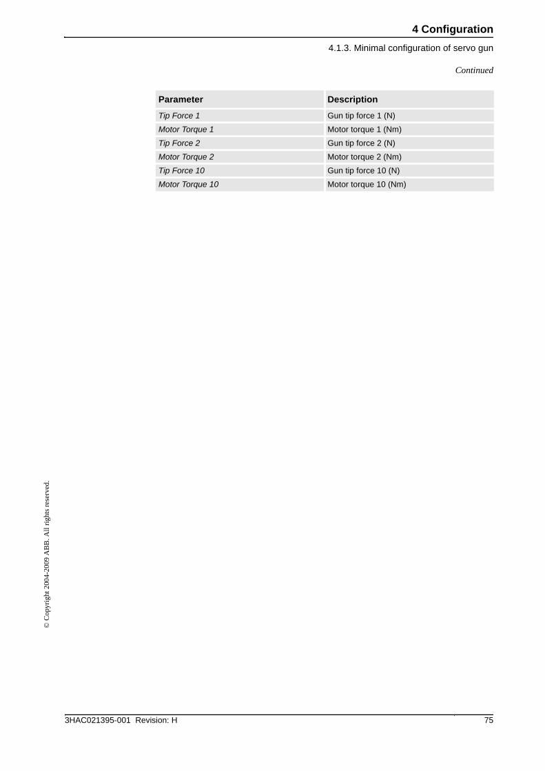
4 Configuration
4.1.3. Minimal configuration of servo gun
753HAC021395-001 Revision: H
© C
opyr
ight
200
4-20
09 A
BB
. All
righ
ts r
eser
ved.
Tip Force 1 Gun tip force 1 (N)
Motor Torque 1 Motor torque 1 (Nm)
Tip Force 2 Gun tip force 2 (N)
Motor Torque 2 Motor torque 2 (Nm)
Tip Force 10 Gun tip force 10 (N)
Motor Torque 10 Motor torque 10 (Nm)
Parameter Description
Continued
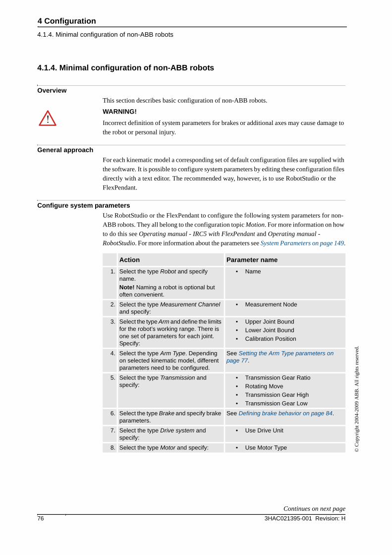
4 Configuration
4.1.4. Minimal configuration of non-ABB robots
3HAC021395-001 Revision: H76
© C
opyr
ight
200
4-20
09 A
BB
. All
righ
ts r
eser
ved.
4.1.4. Minimal configuration of non-ABB robots
Overview
This section describes basic configuration of non-ABB robots.
WARNING!
Incorrect definition of system parameters for brakes or additional axes may cause damage to
the robot or personal injury.
General approach
For each kinematic model a corresponding set of default configuration files are supplied with
the software. It is possible to configure system parameters by editing these configuration files
directly with a text editor. The recommended way, however, is to use RobotStudio or the
FlexPendant.
Configure system parameters
Use RobotStudio or the FlexPendant to configure the following system parameters for non-
ABB robots. They all belong to the configuration topic Motion. For more information on how
to do this see Operating manual - IRC5 with FlexPendant and Operating manual -
RobotStudio. For more information about the parameters see System Parameters on page 149.
Action Parameter name
1. Select the type Robot and specify name.
Note! Naming a robot is optional but often convenient.
• Name
2. Select the type Measurement Channel and specify:
• Measurement Node
3. Select the type Arm and define the limits for the robot’s working range. There is one set of parameters for each joint. Specify:
• Upper Joint Bound
• Lower Joint Bound
• Calibration Position
4. Select the type Arm Type. Depending on selected kinematic model, different parameters need to be configured.
See Setting the Arm Type parameters on page 77.
5. Select the type Transmission and specify:
• Transmission Gear Ratio
• Rotating Move
• Transmission Gear High
• Transmission Gear Low
6. Select the type Brake and specify brake parameters.
See Defining brake behavior on page 84.
7. Select the type Drive system and specify:
• Use Drive Unit
8. Select the type Motor and specify: • Use Motor Type
Continues on next page
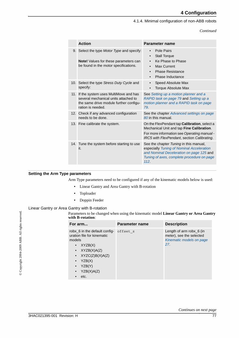
4 Configuration
4.1.4. Minimal configuration of non-ABB robots
773HAC021395-001 Revision: H
© C
opyr
ight
200
4-20
09 A
BB
. All
righ
ts r
eser
ved.
Setting the Arm Type parameters
Arm Type parameters need to be configured if any of the kinematic models below is used:
• Linear Gantry and Area Gantry with B-rotation
• Toploader
• Doppin Feeder
Linear Gantry or Area Gantry with B-rotationParameters to be changed when using the kinematic model Linear Gantry or Area Gantry with B-rotation:
9. Select the type Motor Type and specify:
Note! Values for these parameters can be found in the motor specifications.
• Pole Pairs
• Stall Torque
• Ke Phase to Phase
• Max Current
• Phase Resistance
• Phase Inductance
10. Select the type Stress Duty Cycle and specify:
• Speed Absolute Max
• Torque Absolute Max
11. If the system uses MultiMove and has several mechanical units attached to the same drive module further configu-ration is needed.
See Setting up a motion planner and a RAPID task on page 79 and Setting up a motion planner and a RAPID task on page 79.
12. Check if any advanced configuration needs to be done.
See the chapter Advanced settings on page 80 in this manual.
13. Fine calibrate the system. On the FlexPendant tap Calibration, select a Mechanical Unit and tap Fine Calibration.
For more information see Operating manual - IRC5 with FlexPendant, section Calibrating.
14. Tune the system before starting to use it.
See the chapter Tuning in this manual, especially Tuning of Nominal Acceleration and Nominal Deceleration on page 125 and Tuning of axes, complete procedure on page 112.
Action Parameter name
For arm... Parameter name Description
robx_6 in the default config-uration file for kinematic models
• XYZB(X)
• XYZB(X)A(Z)
• XYZC(Z)B(X)A(Z)
• YZB(X)
• YZB(Y)
• YZB(X)A(Z)
• etc.
offset_z Length of arm robx_6 (in meter), see the selected Kinematic models on page 27.
Continued
Continues on next page
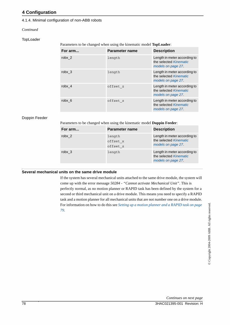
4 Configuration
4.1.4. Minimal configuration of non-ABB robots
3HAC021395-001 Revision: H78
© C
opyr
ight
200
4-20
09 A
BB
. All
righ
ts r
eser
ved.
TopLoaderParameters to be changed when using the kinematic model TopLoader:
Doppin FeederParameters to be changed when using the kinematic model Doppin Feeder:
Several mechanical units on the same drive module
If the system has several mechanical units attached to the same drive module, the system will
come up with the error message 50284 - “Cannot activate Mechanical Unit”. This is
perfectly normal, as no motion planner or RAPID task has been defined by the system for a
second or third mechanical unit on a drive module. This means you need to specify a RAPID
task and a motion planner for all mechanical units that are not number one on a drive module.
For information on how to do this see Setting up a motion planner and a RAPID task on page
79.
For arm... Parameter name Description
robx_2 length Length in meter according to the selected Kinematic models on page 27.
robx_3 length Length in meter according to the selected Kinematic models on page 27.
robx_4 offset_z Length in meter according to the selected Kinematic models on page 27.
robx_6 offset_z Length in meter according to the selected Kinematic models on page 27.
For arm... Parameter name Description
robx_2 length
offset_x
offset_z
Length in meter according to the selected Kinematic models on page 27.
robx_3 length Length in meter according to the selected Kinematic models on page 27.
Continued
Continues on next page
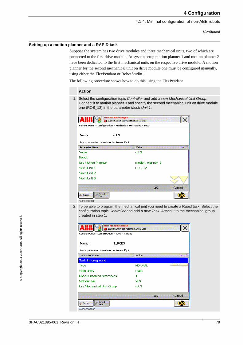
4 Configuration
4.1.4. Minimal configuration of non-ABB robots
793HAC021395-001 Revision: H
© C
opyr
ight
200
4-20
09 A
BB
. All
righ
ts r
eser
ved.
Setting up a motion planner and a RAPID task
Suppose the system has two drive modules and three mechanical units, two of which are
connected to the first drive module. At system setup motion planner 1 and motion planner 2
have been dedicated to the first mechanical units on the respective drive module. A motion
planner for the second mechanical unit on drive module one must be configured manually,
using either the FlexPendant or RobotStudio.
The following procedure shows how to do this using the FlexPendant.
Action
1. Select the configuration topic Controller and add a new Mechanical Unit Group. Connect it to motion planner 3 and specify the second mechanical unit on drive module one (ROB_12) in the parameter Mech Unit 1.
en0600003035
2. To be able to program the mechanical unit you need to create a Rapid task. Select the configuration topic Controller and add a new Task. Attach it to the mechanical group created in step 1.
en0600003036
Continued
4 Configuration
4.2.1. Disconnect a servo motor
3HAC021395-001 Revision: H80
© C
opyr
ight
200
4-20
09 A
BB
. All
righ
ts r
eser
ved.
4.2 Advanced settings
4.2.1. Disconnect a servo motor
Overview
It is possible to disconnect and reconnect the motor of a deactivated axis if a certain
deactivation mode is setup.
NOTE!
If the axis is moved when disconnected, the position of the axis might be wrong after
reconnecting, and this will not be detected by the controller. The position after reconnection
will be correct if the axis is not moved, or if the movement is less than 0.5 motor revolutions.
For servo guns, there is a RAPID calibration method available (the ToolChange calibration)
that will adjust any positional error caused by gun movement during disconnection.
Configure parameters
Use RobotStudio to perform the following instructions. See Operating manual - RobotStudio
For parameter description, see chapter System Parameters on page 149.
Action Info/Illustration
1. Select the topic Motion and type Measurement channel and define the following in the parameter.
• Disconnect at Deactive
4 Configuration
4.2.2. Servo Tool Change
813HAC021395-001 Revision: H
© C
opyr
ight
200
4-20
09 A
BB
. All
righ
ts r
eser
ved.
4.2.2. Servo Tool Change
Overview
With the option 630-1, Servo Tool Change, it is possible to disconnect the resolver and power
cables from the motor of one external axis and connect them to the motor of another
additional axis.
For details about Servo Tool Change, see Application manual - Servo motor control.
WARNING!
It is important that no other mechanical unit used with one tool changer are activated, but the
one corresponding to the currently connected servo gun! An activation of the wrong
mechanical unit may cause unexpected movements and personal injury. See Defining relays
on page 83.
NOTE!
In case the Servo Gun is equipped with a brake, the 24V to the brake must be switched off
before and during servo tool change. This is done via an I/O -signal and brake relay (e.g. by
using the instruction WaitTime on the brake relay). See Defining relays on page 83, for
defining of brake relays.
Considerations
The list below specifies special considerations when switching motors:
• The two (or more) additional axes sharing the same motor cables are configured as
separate mechanical units.
• The additional axes are configured to use the same measurement node and drive unit
node.
• If two servo guns are used with a tool changer, the template file M7L1B1S_DM1.cfg
can be used for configuration of both guns.
• A motor switch can be done only if all sharing axes are deactivated.
• The reconnected motor is activated and this activation will restore the position of the
axis to the latest position.
• A new motor switch cannot be performed until this axis is deactivated.
• Always use the tool change tip calibration after activation.
Connection Relay
To make sure that the correct mechanical unit is active, some tool changers support I/O
signals that specify which gun is currently connected.
It is also possible to lock unconnected mechanical units from activation by specifying a
connection relay and connect it to a digital input (DI).
Continues on next page
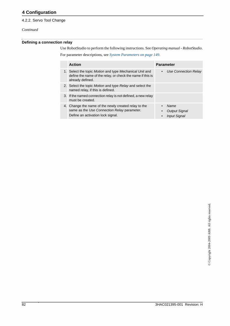
4 Configuration
4.2.2. Servo Tool Change
3HAC021395-001 Revision: H82
© C
opyr
ight
200
4-20
09 A
BB
. All
righ
ts r
eser
ved.
Defining a connection relay
Use RobotStudio to perform the following instructions. See Operating manual - RobotStudio.
For parameter descriptions, see System Parameters on page 149.
Action Parameter
1. Select the topic Motion and type Mechanical Unit and define the name of the relay, or check the name if this is already defined.
• Use Connection Relay
2. Select the topic Motion and type Relay and select the named relay, if this is defined.
3. If the named connection relay is not defined, a new relay must be created.
4. Change the name of the newly created relay to the same as the Use Connection Relay parameter.
Define an activation lock signal.
• Name
• Output Signal
• Input Signal
Continued
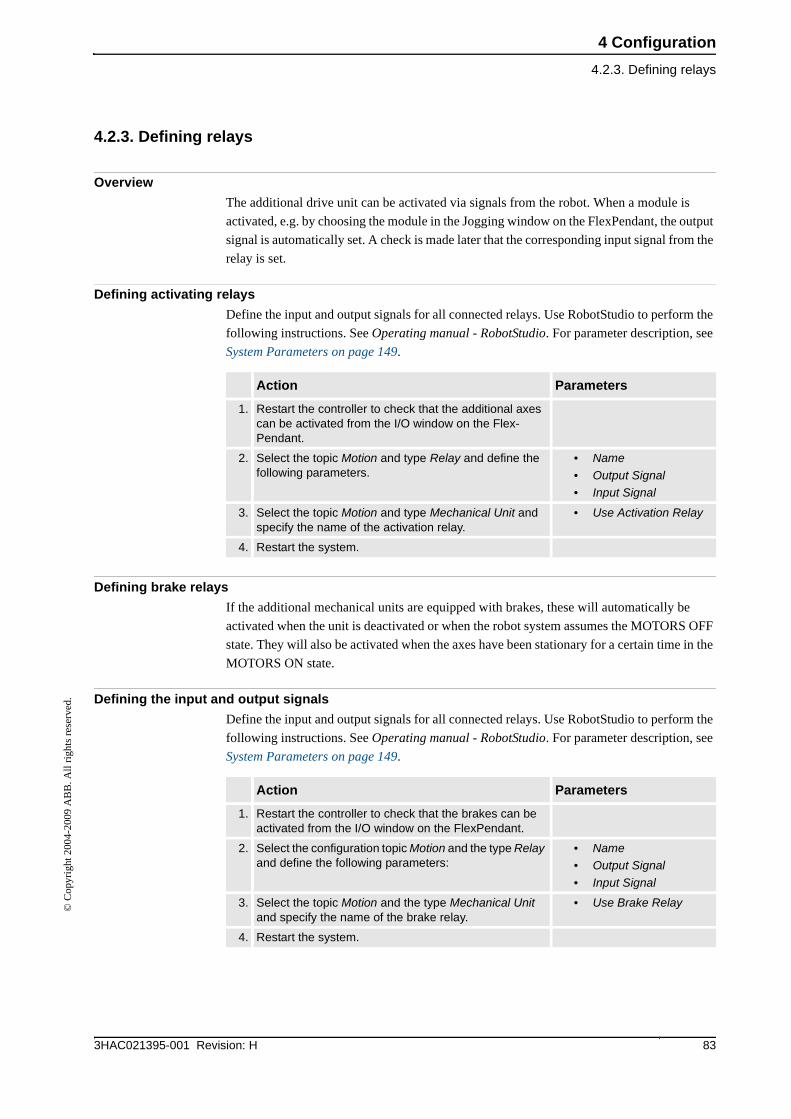
4 Configuration
4.2.3. Defining relays
833HAC021395-001 Revision: H
© C
opyr
ight
200
4-20
09 A
BB
. All
righ
ts r
eser
ved.
4.2.3. Defining relays
Overview
The additional drive unit can be activated via signals from the robot. When a module is
activated, e.g. by choosing the module in the Jogging window on the FlexPendant, the output
signal is automatically set. A check is made later that the corresponding input signal from the
relay is set.
Defining activating relays
Define the input and output signals for all connected relays. Use RobotStudio to perform the
following instructions. See Operating manual - RobotStudio. For parameter description, see
System Parameters on page 149.
Defining brake relays
If the additional mechanical units are equipped with brakes, these will automatically be
activated when the unit is deactivated or when the robot system assumes the MOTORS OFF
state. They will also be activated when the axes have been stationary for a certain time in the
MOTORS ON state.
Defining the input and output signals
Define the input and output signals for all connected relays. Use RobotStudio to perform the
following instructions. See Operating manual - RobotStudio. For parameter description, see
System Parameters on page 149.
Action Parameters
1. Restart the controller to check that the additional axes can be activated from the I/O window on the Flex-Pendant.
2. Select the topic Motion and type Relay and define the following parameters.
• Name
• Output Signal
• Input Signal
3. Select the topic Motion and type Mechanical Unit and specify the name of the activation relay.
• Use Activation Relay
4. Restart the system.
Action Parameters
1. Restart the controller to check that the brakes can be activated from the I/O window on the FlexPendant.
2. Select the configuration topic Motion and the type Relay and define the following parameters:
• Name
• Output Signal
• Input Signal
3. Select the topic Motion and the type Mechanical Unit and specify the name of the brake relay.
• Use Brake Relay
4. Restart the system.
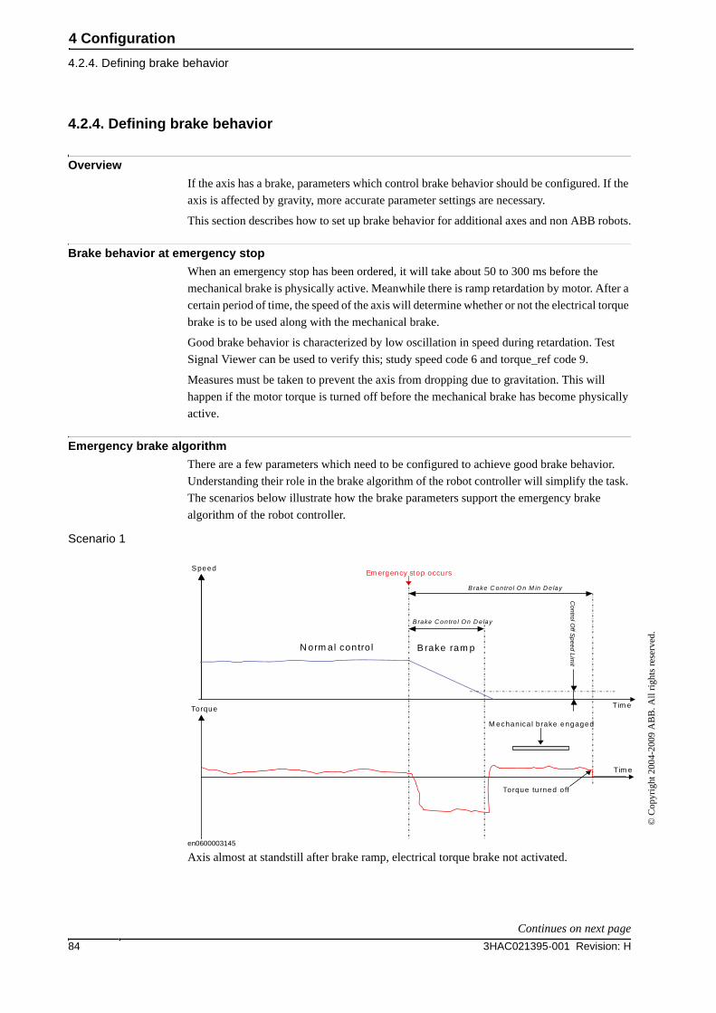
4 Configuration
4.2.4. Defining brake behavior
3HAC021395-001 Revision: H84
© C
opyr
ight
200
4-20
09 A
BB
. All
righ
ts r
eser
ved.
4.2.4. Defining brake behavior
Overview
If the axis has a brake, parameters which control brake behavior should be configured. If the
axis is affected by gravity, more accurate parameter settings are necessary.
This section describes how to set up brake behavior for additional axes and non ABB robots.
Brake behavior at emergency stop
When an emergency stop has been ordered, it will take about 50 to 300 ms before the
mechanical brake is physically active. Meanwhile there is ramp retardation by motor. After a
certain period of time, the speed of the axis will determine whether or not the electrical torque
brake is to be used along with the mechanical brake.
Good brake behavior is characterized by low oscillation in speed during retardation. Test
Signal Viewer can be used to verify this; study speed code 6 and torque_ref code 9.
Measures must be taken to prevent the axis from dropping due to gravitation. This will
happen if the motor torque is turned off before the mechanical brake has become physically
active.
Emergency brake algorithm
There are a few parameters which need to be configured to achieve good brake behavior.
Understanding their role in the brake algorithm of the robot controller will simplify the task.
The scenarios below illustrate how the brake parameters support the emergency brake
algorithm of the robot controller.
Scenario 1
en0600003145
Axis almost at standstill after brake ramp, electrical torque brake not activated.
N orm al contro l B rake ram p
M echanica l brake engaged
Torque turned o ff
Em ergency stop occursSpeed
Torque Tim e
Tim e
Brake C ontro l O n M in D e lay
Brake C ontro l O n D e lay
Control O
ff Speed Lim
it
Continues on next page
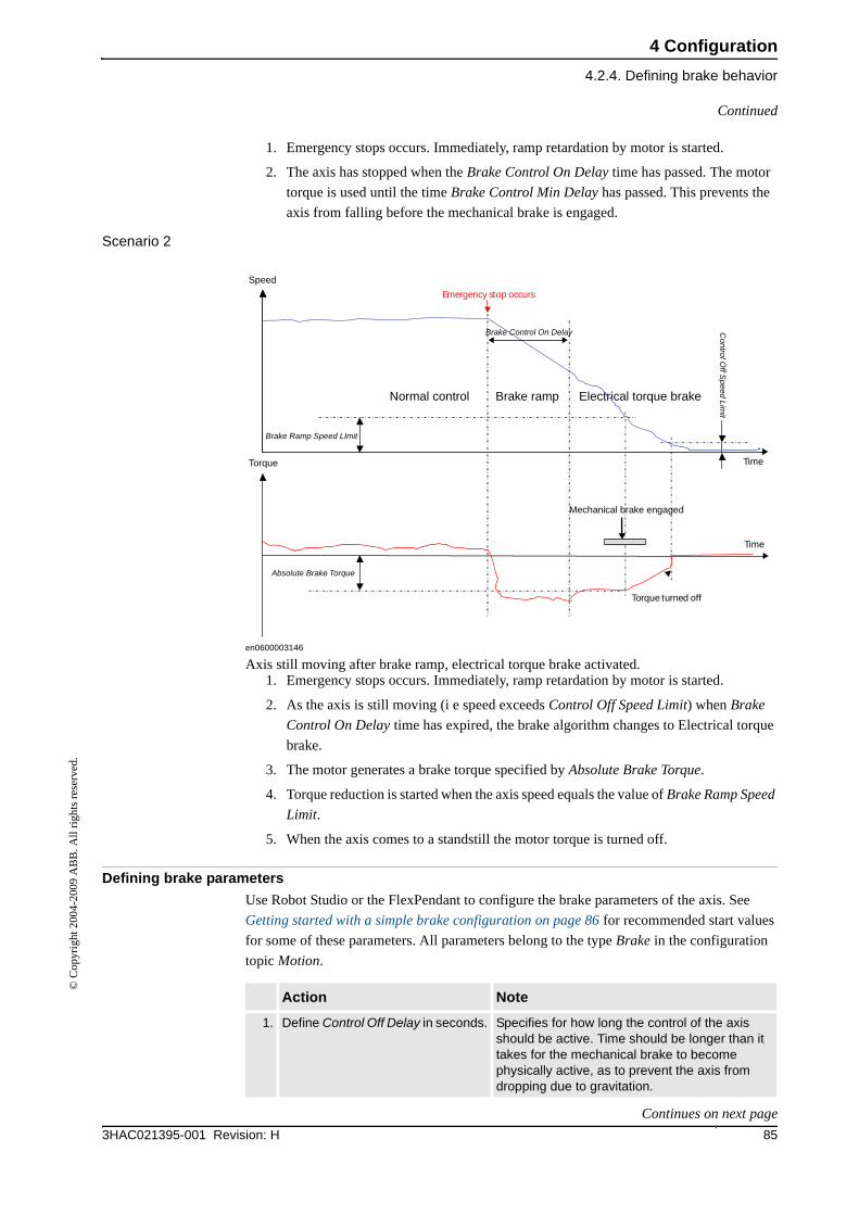
4 Configuration
4.2.4. Defining brake behavior
853HAC021395-001 Revision: H
© C
opyr
ight
200
4-20
09 A
BB
. All
righ
ts r
eser
ved.
1. Emergency stops occurs. Immediately, ramp retardation by motor is started.
2. The axis has stopped when the Brake Control On Delay time has passed. The motor
torque is used until the time Brake Control Min Delay has passed. This prevents the
axis from falling before the mechanical brake is engaged.
Scenario 2
en0600003146
Axis still moving after brake ramp, electrical torque brake activated.1. Emergency stops occurs. Immediately, ramp retardation by motor is started.
2. As the axis is still moving (i e speed exceeds Control Off Speed Limit) when Brake
Control On Delay time has expired, the brake algorithm changes to Electrical torque
brake.
3. The motor generates a brake torque specified by Absolute Brake Torque.
4. Torque reduction is started when the axis speed equals the value of Brake Ramp Speed
Limit.
5. When the axis comes to a standstill the motor torque is turned off.
Defining brake parameters
Use Robot Studio or the FlexPendant to configure the brake parameters of the axis. See
Getting started with a simple brake configuration on page 86 for recommended start values
for some of these parameters. All parameters belong to the type Brake in the configuration
topic Motion.
Normal control Brake ramp Electrical torque brake
Speed
Torque Time
Time
Mechanical brake engaged
Torque turned off
Emergency stop occurs
Brake Control On Delay
Brake Ramp Speed LImit
Absolute Brake Torque
Control O
ff Speed Lim
it
Action Note
1. Define Control Off Delay in seconds. Specifies for how long the control of the axis should be active. Time should be longer than it takes for the mechanical brake to become physically active, as to prevent the axis from dropping due to gravitation.
Continued
Continues on next page
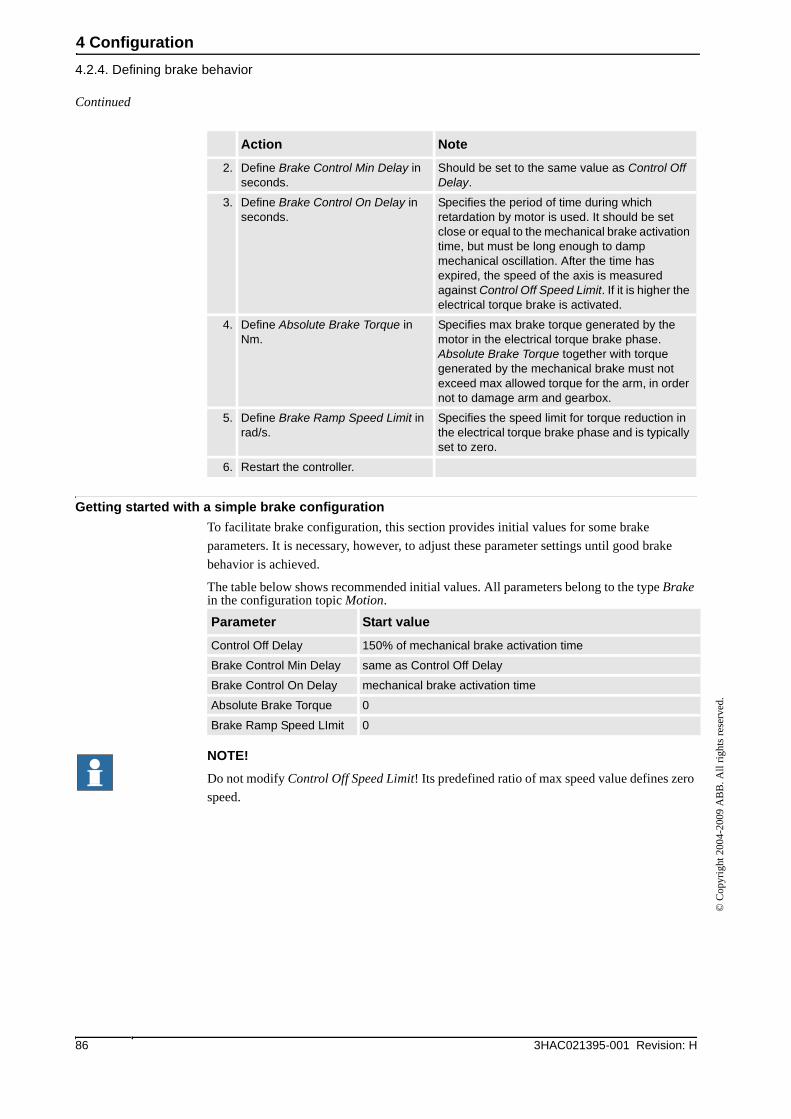
4 Configuration
4.2.4. Defining brake behavior
3HAC021395-001 Revision: H86
© C
opyr
ight
200
4-20
09 A
BB
. All
righ
ts r
eser
ved.
Getting started with a simple brake configuration
To facilitate brake configuration, this section provides initial values for some brake
parameters. It is necessary, however, to adjust these parameter settings until good brake
behavior is achieved.
The table below shows recommended initial values. All parameters belong to the type Brake in the configuration topic Motion.
NOTE!
Do not modify Control Off Speed Limit! Its predefined ratio of max speed value defines zero
speed.
2. Define Brake Control Min Delay in seconds.
Should be set to the same value as Control Off Delay.
3. Define Brake Control On Delay in seconds.
Specifies the period of time during which retardation by motor is used. It should be set close or equal to the mechanical brake activation time, but must be long enough to damp mechanical oscillation. After the time has expired, the speed of the axis is measured against Control Off Speed Limit. If it is higher the electrical torque brake is activated.
4. Define Absolute Brake Torque in Nm.
Specifies max brake torque generated by the motor in the electrical torque brake phase. Absolute Brake Torque together with torque generated by the mechanical brake must not exceed max allowed torque for the arm, in order not to damage arm and gearbox.
5. Define Brake Ramp Speed Limit in rad/s.
Specifies the speed limit for torque reduction in the electrical torque brake phase and is typically set to zero.
6. Restart the controller.
Action Note
Parameter Start value
Control Off Delay 150% of mechanical brake activation time
Brake Control Min Delay same as Control Off Delay
Brake Control On Delay mechanical brake activation time
Absolute Brake Torque 0
Brake Ramp Speed LImit 0
Continued
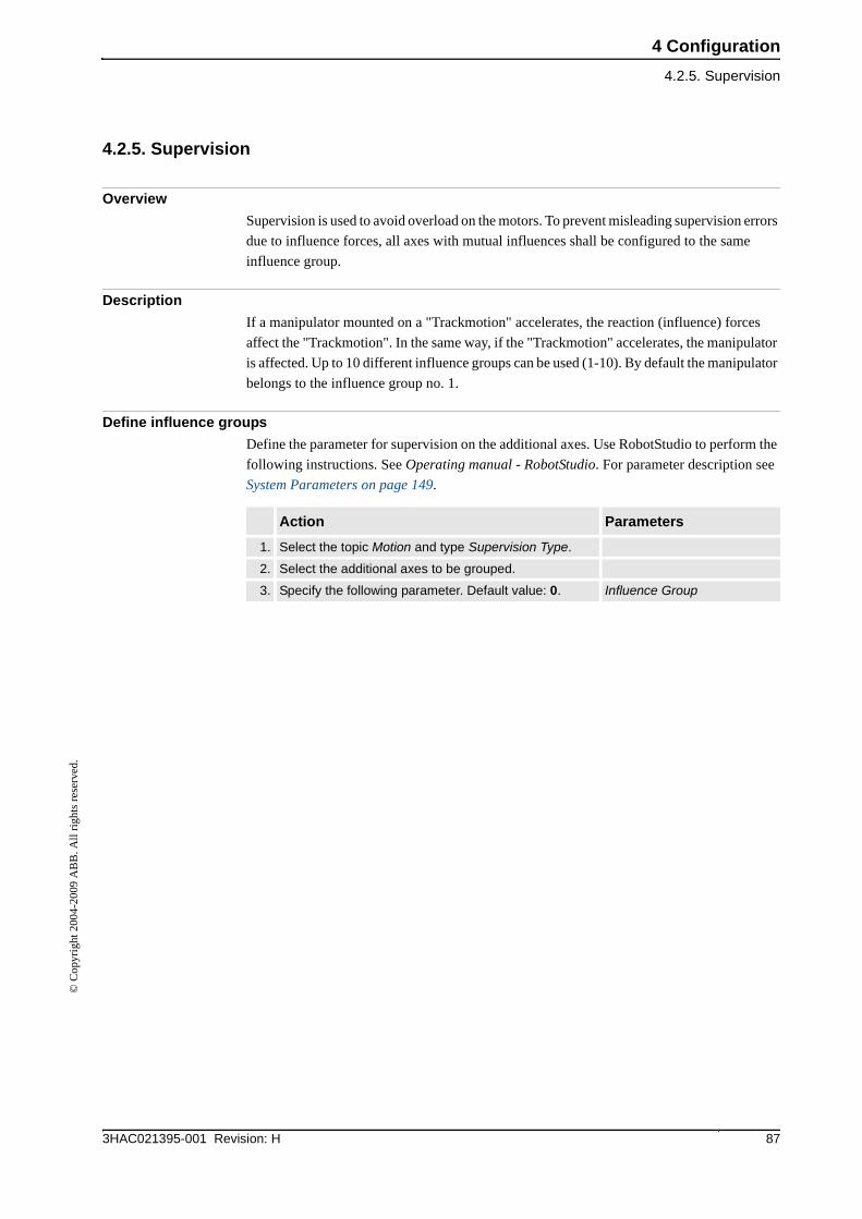
4 Configuration
4.2.5. Supervision
873HAC021395-001 Revision: H
© C
opyr
ight
200
4-20
09 A
BB
. All
righ
ts r
eser
ved.
4.2.5. Supervision
Overview
Supervision is used to avoid overload on the motors. To prevent misleading supervision errors
due to influence forces, all axes with mutual influences shall be configured to the same
influence group.
Description
If a manipulator mounted on a "Trackmotion" accelerates, the reaction (influence) forces
affect the "Trackmotion". In the same way, if the "Trackmotion" accelerates, the manipulator
is affected. Up to 10 different influence groups can be used (1-10). By default the manipulator
belongs to the influence group no. 1.
Define influence groups
Define the parameter for supervision on the additional axes. Use RobotStudio to perform the
following instructions. See Operating manual - RobotStudio. For parameter description see
System Parameters on page 149.
Action Parameters
1. Select the topic Motion and type Supervision Type.
2. Select the additional axes to be grouped.
3. Specify the following parameter. Default value: 0. Influence Group
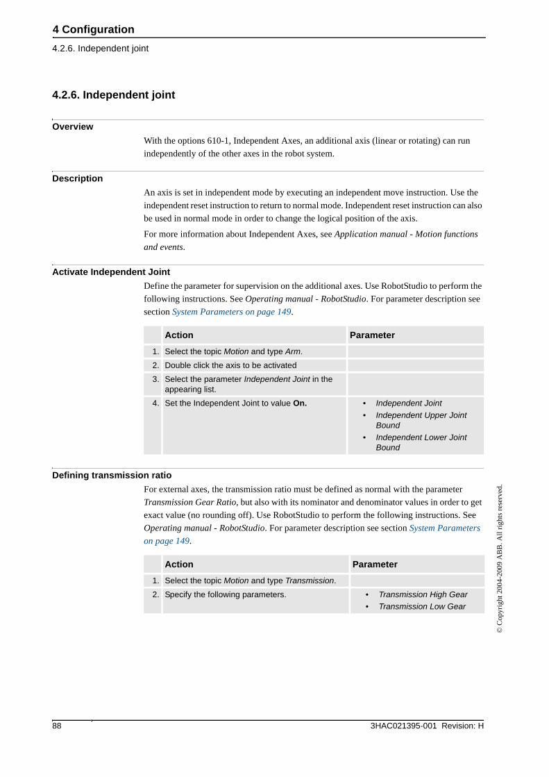
4 Configuration
4.2.6. Independent joint
3HAC021395-001 Revision: H88
© C
opyr
ight
200
4-20
09 A
BB
. All
righ
ts r
eser
ved.
4.2.6. Independent joint
Overview
With the options 610-1, Independent Axes, an additional axis (linear or rotating) can run
independently of the other axes in the robot system.
Description
An axis is set in independent mode by executing an independent move instruction. Use the
independent reset instruction to return to normal mode. Independent reset instruction can also
be used in normal mode in order to change the logical position of the axis.
For more information about Independent Axes, see Application manual - Motion functions
and events.
Activate Independent Joint
Define the parameter for supervision on the additional axes. Use RobotStudio to perform the
following instructions. See Operating manual - RobotStudio. For parameter description see
section System Parameters on page 149.
Defining transmission ratio
For external axes, the transmission ratio must be defined as normal with the parameter
Transmission Gear Ratio, but also with its nominator and denominator values in order to get
exact value (no rounding off). Use RobotStudio to perform the following instructions. See
Operating manual - RobotStudio. For parameter description see section System Parameters
on page 149.
Action Parameter
1. Select the topic Motion and type Arm.
2. Double click the axis to be activated
3. Select the parameter Independent Joint in the appearing list.
4. Set the Independent Joint to value On. • Independent Joint
• Independent Upper Joint Bound
• Independent Lower Joint Bound
Action Parameter
1. Select the topic Motion and type Transmission.
2. Specify the following parameters. • Transmission High Gear
• Transmission Low Gear
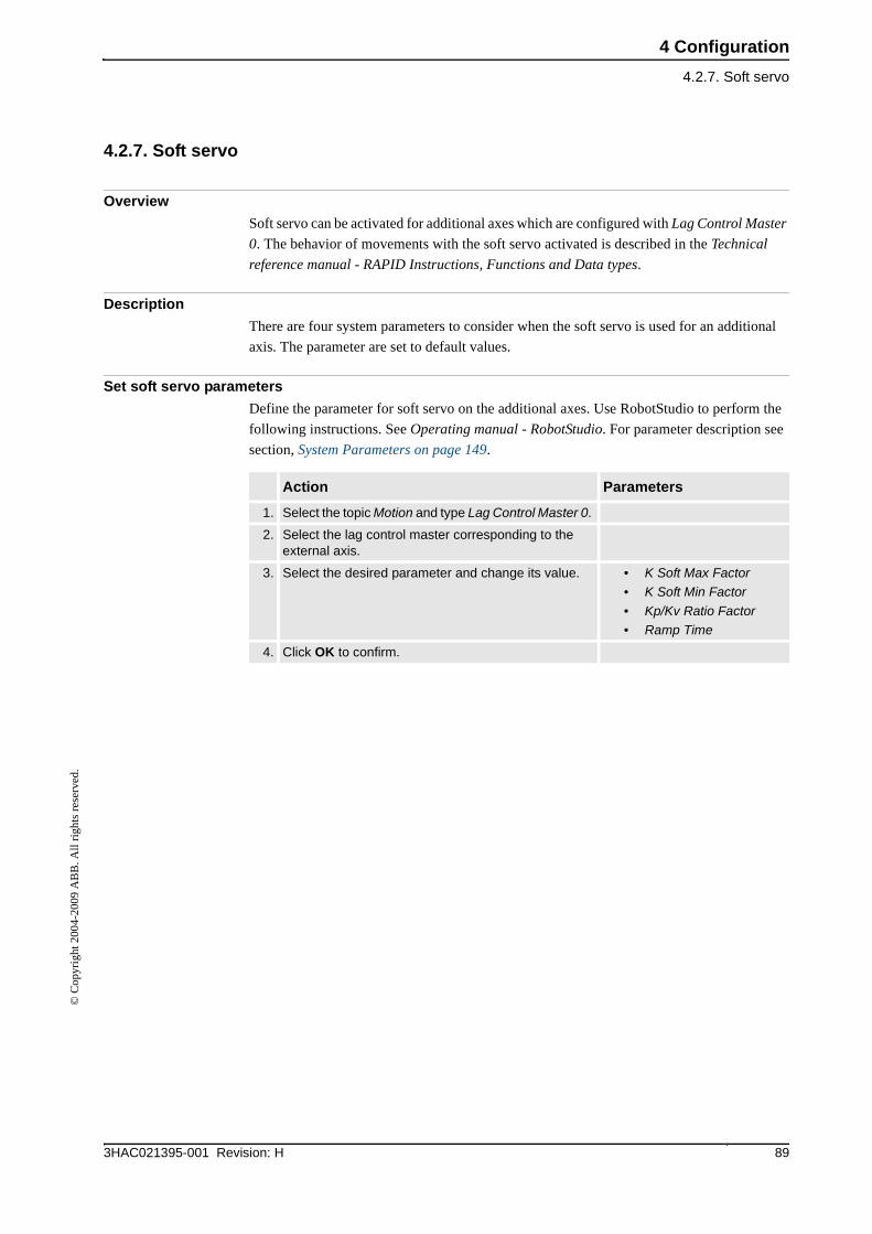
4 Configuration
4.2.7. Soft servo
893HAC021395-001 Revision: H
© C
opyr
ight
200
4-20
09 A
BB
. All
righ
ts r
eser
ved.
4.2.7. Soft servo
Overview
Soft servo can be activated for additional axes which are configured with Lag Control Master
0. The behavior of movements with the soft servo activated is described in the Technical
reference manual - RAPID Instructions, Functions and Data types.
Description
There are four system parameters to consider when the soft servo is used for an additional
axis. The parameter are set to default values.
Set soft servo parameters
Define the parameter for soft servo on the additional axes. Use RobotStudio to perform the
following instructions. See Operating manual - RobotStudio. For parameter description see
section, System Parameters on page 149.
Action Parameters
1. Select the topic Motion and type Lag Control Master 0.
2. Select the lag control master corresponding to the external axis.
3. Select the desired parameter and change its value. • K Soft Max Factor
• K Soft Min Factor
• Kp/Kv Ratio Factor
• Ramp Time
4. Click OK to confirm.
4 Configuration
4.2.8. Activate force gain control
3HAC021395-001 Revision: H90
© C
opyr
ight
200
4-20
09 A
BB
. All
righ
ts r
eser
ved.
4.2.8. Activate force gain control
Overview
Force gain control is used in cases when heavy load, high friction and low speed makes it
difficult for an additional axis to reach its end point.
All axes that affect force gain control must be within a certain position range from the end
point before forced gain control is enabled. This position range is also specified in the
configuration topic Motion, type Supervision.
Description
When activating forced gain control for an additional axis, two types under Motion must be
considered. Decide which axes should have forced gain control in Lag Control Master 0, and
decide which axes should affect forced gain control in Supervision.
Set force gain control parameters
Define the parameter for forced gain control on the additional axes. Use RobotStudio to
perform the following instructions. See Operating manual - RobotStudio. For parameter
description see section, System Parameters on page 149.
Set supervision parameters
Define the parameter for supervision on the additional axes. Use RobotStudio to perform the
following instructions. See Operating manual - RobotStudio. For parameter description see
section, System Parameters on page 149.
CAUTION!
Do not change supervision for the robot axes. Changes on these values could affect the service
interval cycles and impair its performance.
Action Parameter
1. Select the topic Motion and type Lag Control Master 0.
2. Select the lag control master corresponding to the additional axis.
3. Select the parameter to be changed. • Forced Control Active
• Forced Factor for Kp
• Forced Factor for Ki
• Rise Time for Kp
4. Press: OK to confirm.
Action Parameter
1. Select the topic Motion and type Supervision.
2. Select the lag control master corresponding to the axis that should or should not affect forced gain control.
3. Select the parameter to be changed. • Affects Forced Control
• Forced on Position Limit
• Forced off Position Limit
4. Click OK to confirm.
4 Configuration
4.2.9. Activate notch filter
913HAC021395-001 Revision: H
© C
opyr
ight
200
4-20
09 A
BB
. All
righ
ts r
eser
ved.
4.2.9. Activate notch filter
Overview
The notch filter is used to prevent the additional axis from oscillating at the weave motion
frequency.
The notch filter is used only in arc welding applications when a variation in additional axis
speed affects the welding process. This problem occurs when both coordinated interpolation
and weaving are used. The frequency of the speed variation is typically 2 times the weaving
frequency.
Description
There are two ways to use the notch filter:
• Lock the notch filter to one specific frequency specified in the parameter Notch Filter
Frequency.
• Activate Notch Auto Mode, which means that the notch filter will automatically adjust
to the current weave frequency.
NOTE!
A notch filter should not be used together with Rapid Weave. In Notch Auto Mode this is
handled automatically and as if there was no weaving at all.
Activate notch filter
To activate notch filter for an additional axis. Use RobotStudio to perform the following
instructions. See Operating manual - RobotStudio. For parameter description see
sectionSystem Parameters on page 149.
Action Parameters
1. Select the topic Motion and type Lag Control Master 0.
2. Select the lag control master corresponding to the additional axis.
3. Select the desired parameter and change its value. • Notch Filter Activated
• Notch Filter Frequency
• Notch Filter Width
• Notch Auto Mode
• Auto No Weave Frequency
• Auto Min Frequency
• Auto Max Relative Change
4. Click OK to confirm.
4 Configuration
4.2.10. Defining kinematic parameters for general kinematics
3HAC021395-001 Revision: H92
© C
opyr
ight
200
4-20
09 A
BB
. All
righ
ts r
eser
ved.
4.2.10. Defining kinematic parameters for general kinematics
Overview
It is possible to use general kinematic for all robots and positioners. There are no standard
configuration files for positioners available.
NOTE!
Definition is not possible via the FlexPendant, PC editing of the MOC.cfg file is necessary.
Positioners
The following needs to be defined.
Type Description
ROBOT_TYPE • base_pose_rot_u0, base_pose_rot_u1, base_pose_rot_u2, base_pose_rot_u3 (Rotation between user defined robot base and internal base according to Denavit - Hartenberg definition).
• no_of_joints = highest joint number
• type GEN_KIN
ARM For each arm of the additional robot in question.
• rotating_move if rotating axes, exclude otherwise
ARM_TYPE For each arm of the external robot in question.
• length (a according to Craigh’s definition)
• offset_x = 0
• offset_y = 0
• theta_home_position (theta according to Craigh’s definition)
• offset_z (d according to Craigh’s definition)
• attitude (alpha according to Craigh’s definition)
4 Configuration
4.3.1. About coordinated axes
933HAC021395-001 Revision: H
© C
opyr
ight
200
4-20
09 A
BB
. All
righ
ts r
eser
ved.
4.3 Coordinated axes
4.3.1. About coordinated axes
Additional axes, general
All additional axes are handled in mechanical units. This means that before an additional axis
may be moved, the mechanical unit to which it belongs, must be activated. Within a
mechanical unit, the different axes will be given a logical name, from a to f. In the system
parameters, these logical axes will be connected to the additional axes joints. For each joint
a motor and a drive unit is defined. Different joints may share the same motor and drive unit.
Two or more mechanical units may be activated at the same time, as long as they do not have
the same logical axes defined in their set of additional axes. However, two or more
mechanical units may have the same logical axes, if they are not activated simultaneously.
Two or more mechanical units may not be activated at the same time, if they share one or
more drive units, even if they use separate logical axes. This means that two logical axes, each
belonging to different mechanical units, may control the same drive unit, but not at the same
time.
Coordination
A mechanical unit may be coordinated or not coordinated with the robot movements. If it is
not coordinated, each axis will be moved independent of the robot movements, e.g. when
jogging, only the separate axis will move. However during program execution, the additional
axes will be synchronized to the robot movement, in such a way that both movements will be
completed in the same time.
If the mechanical unit is coordinated, the TCP velocity in the object coordinate system, will
be the programmed velocity irrespective of the movements of the additional axes. Two types
of coordination categories exist. The first category of coordination is when the robot base is
moved, e.g. the coordination to a gantry or track movement. This means that the robot is
mounted on a gantry or a track, and may be moved along these axes. The world and user/
object coordinate systems, however, will be fixed in the room, and the robot movements in
these coordinate systems will be independent of simultaneous gantry or track movements.
This coordination is automatically active, if the mechanical unit with the track motion is
active.
The second coordination category, is when the robot movements are coordinated to the
movements of a user frame connected to a mechanical unit. E.g. a user frame may be placed
on a turntable and connected to its movements. An ordinary work object may be used for this
purpose, if it is marked with the name of the mechanical unit to be connected to, and that it
should be moveable. The coordination will be active if the mechanical unit is active, and the
coordinated work object is active. When such a coordinated work object is used, in jogging
or in a move instruction, the data in the uframe component will be ignored and the location
of the user coordinate system will only depend on the movements of the mechanical unit.
However the oframe component will still work giving an object frame related to the user
frame and also the displacement frame may be used.
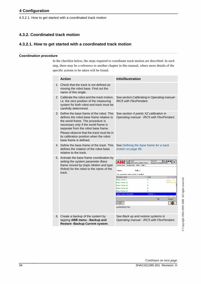
4 Configuration
4.3.2.1. How to get started with a coordinated track motion
3HAC021395-001 Revision: H94
© C
opyr
ight
200
4-20
09 A
BB
. All
righ
ts r
eser
ved.
4.3.2. Coordinated track motion
4.3.2.1. How to get started with a coordinated track motion
Coordination procedure
In the checklist below, the steps required to coordinate track motion are described. In each
step, there may be a reference to another chapter in this manual, where more details of the
specific actions to be taken will be found.
Action Info/illustration
1. Check that the track is not defined as moving the robot base. Find out the name of this single.
2. Calibrate the robot and the track motion, i.e. the zero position of the measuring system for both robot and track must be carefully determined.
See section Calibrating in Operating manual - IRC5 with FlexPendant.
3. Define the base frame of the robot. This defines the robot base frame relative to the world frame. The procedure is necessary only if the world frame is separate from the robot base frame.
Please observe that the track must be in its calibration position when the robot base frame is defined.
See section 4 points XZ calibration in Operating manual - IRC5 with FlexPendant.
4. Define the base frame of the track. This defines the rotation of the robot base relative to the track.
See Defining the base frame for a track motion on page 96.
5. Activate the base frame coordination by setting the system parameter Base frame moved by (topic Motion and type Robot) for the robot to the name of the track.
en0600002756
6. Create a backup of the system by tapping ABB menu - Backup and Restore -Backup Current system.
See Back up and restore systems in Operating manual - IRC5 with FlexPendant.
Continues on next page
4 Configuration
4.3.2.1. How to get started with a coordinated track motion
953HAC021395-001 Revision: H
© C
opyr
ight
200
4-20
09 A
BB
. All
righ
ts r
eser
ved.
NOTE!
If the robot base frame is rotated after the calibration of the track base frame, a new base
frame calibration of the robot has to be done and also a new baseframe calibration of the track.
7. Activate the track unit in the jogging window and check that the coordination is working satisfactorily.
This may be done by choosing World or Work Object in the field Coordinate System and then jogging the track axis. The robot TCP should not move, but be fixed relative to the object coordinate system.
Action Info/illustration
Continued
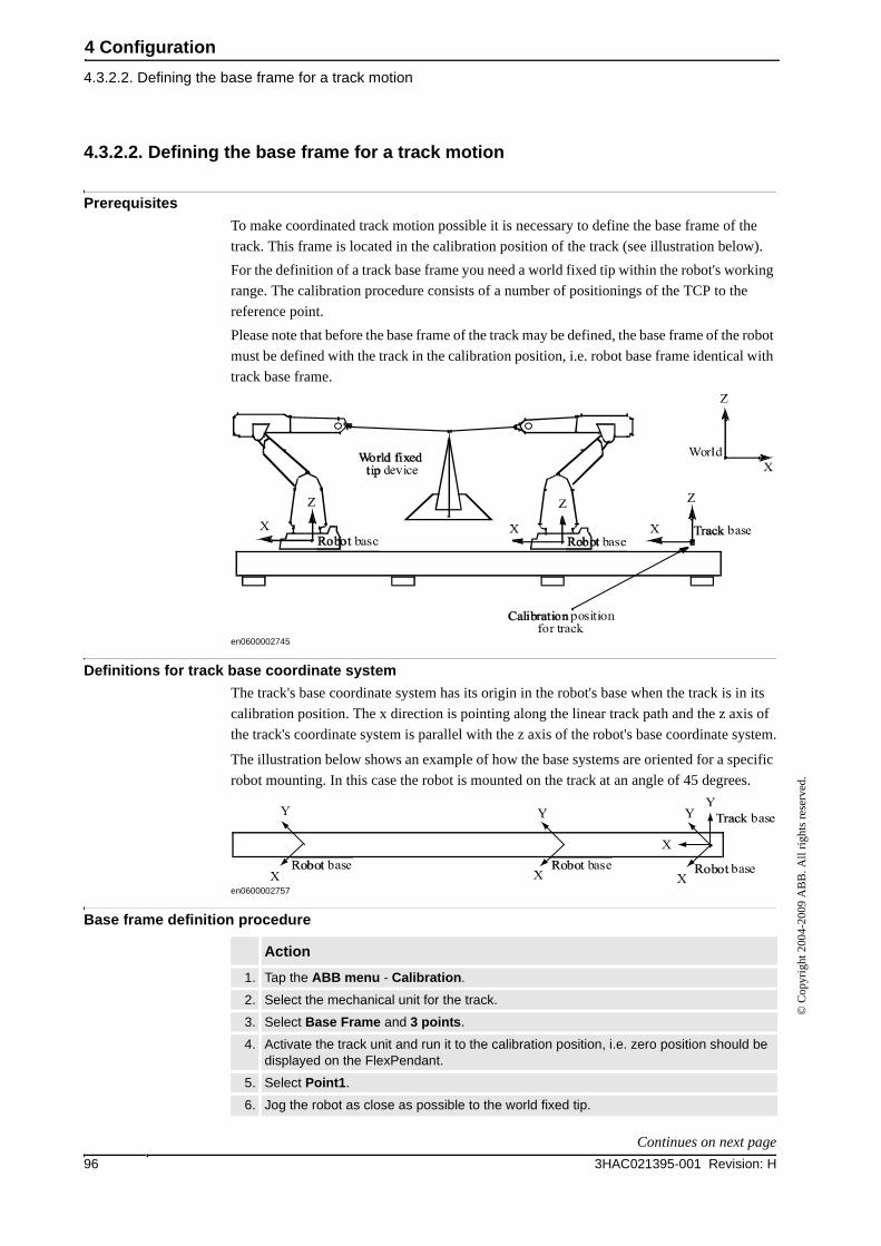
4 Configuration
4.3.2.2. Defining the base frame for a track motion
3HAC021395-001 Revision: H96
© C
opyr
ight
200
4-20
09 A
BB
. All
righ
ts r
eser
ved.
4.3.2.2. Defining the base frame for a track motion
Prerequisites
To make coordinated track motion possible it is necessary to define the base frame of the
track. This frame is located in the calibration position of the track (see illustration below).
For the definition of a track base frame you need a world fixed tip within the robot's working
range. The calibration procedure consists of a number of positionings of the TCP to the
reference point.
Please note that before the base frame of the track may be defined, the base frame of the robot
must be defined with the track in the calibration position, i.e. robot base frame identical with
track base frame.
en0600002745
Definitions for track base coordinate system
The track's base coordinate system has its origin in the robot's base when the track is in its
calibration position. The x direction is pointing along the linear track path and the z axis of
the track's coordinate system is parallel with the z axis of the robot's base coordinate system.
The illustration below shows an example of how the base systems are oriented for a specific
robot mounting. In this case the robot is mounted on the track at an angle of 45 degrees.
en0600002757
Base frame definition procedure
Action
1. Tap the ABB menu - Calibration.
2. Select the mechanical unit for the track.
3. Select Base Frame and 3 points.
4. Activate the track unit and run it to the calibration position, i.e. zero position should be displayed on the FlexPendant.
5. Select Point1.
6. Jog the robot as close as possible to the world fixed tip.
Continues on next page
4 Configuration
4.3.2.2. Defining the base frame for a track motion
973HAC021395-001 Revision: H
© C
opyr
ight
200
4-20
09 A
BB
. All
righ
ts r
eser
ved.
Result
The result of the calculation is displayed (expressed in the world coordinate system). The
following values are shown:
If the estimated error is acceptable, press OK to confirm the new track base frame.
If the estimated error is unacceptable, press Cancel to redefine the calibration.
7. Modify the position by tapping Modify Position.
8. Move the robot along the track and repeat the steps above for the points Point 2 and Point 3.
9. Press OK to calculate the base frame for the track.
Action
Listed values Description
Method Displays the selected calibration method.
Max error The maximum error for one positioning.
Min error The minimum error for one positioning.
Mean error The accuracy of the robot positioning against the tip.
Cartesian X The x coordinate for the base frame. (x, y, z is the same as for the robot base frame).
Cartesian Y The y coordinate for the base frame.
Cartesian Z The z coordinate for the base frame.
Quaternion 1-4 Orientation components for the base frame
Continued
4 Configuration
4.3.3.1. How to get started with a coordinated (moveable) user coordinate system
3HAC021395-001 Revision: H98
© C
opyr
ight
200
4-20
09 A
BB
. All
righ
ts r
eser
ved.
4.3.3. Coordinated positioners
4.3.3.1. How to get started with a coordinated (moveable) user coordinate system
Coordination procedure
In the checklist below, the steps required to coordinate a user coordinate system are described.
In each step, there may be a reference to another chapter in this manual, where more details
of the specific actions to be taken will be found.
TIP!
When programming, it is important to have the coordinated work object, in this case
wobj_turntable, programmed as an argument in each move instruction. This will be
automatically added to the move instruction, if the work object is activated in the jogging
window before starting the programming.
Action Info
1. Calibrate the robot and the positioner, i.e. the zero position of the measuring system for both robot and positioner must be carefully determined.
See section Calibrating in Operating manual - IRC5 with FlexPendant.
2. Define the base frame of the robot. See 4 points XZ calibration in Operating manual - IRC5 with FlexPendant.
3. Define the user frame of the positioner. See Defining the user frame for a rotational single axis on page 99, or Defining the user frame for a multi axes positioner on page 102.
4. Create a backup of the system by tapping ABB - Backup and Restore -Backup Current system.
See Back up and restore systems in Operating manual - IRC5 with FlexPendant.
5. Create a new work object data and give it a name, e.g. wobj_turntable.
In this work object, change the component ufprog to FALSE, indicating that the user object should be connected to a moveable mechanical unit. Also change the component ufmec to the name of the positioner (e.g. STN_1).
See section Creating a work object in Operating manual - IRC5 with FlexPendant.
6. If you want the object frame to be displaced relative to the user frame, you may write the displacement in the x, y, z values of the oframe component of the work object.
For more information about the object frame, see Operating manual - IRC5 with FlexPendant, section What is a work object and section Defining the work object coordinate system.
7. Activate the positioner in the jogging window and check that the coordination is working satisfactorily.
This can be done by:
• selecting Work Object in the field Coordinate system
• selecting your work object, e.g. wobj_turntable, in the field Work object
When jogging the positioner, the robot TCP should also move, following the moveable object coordinate system.
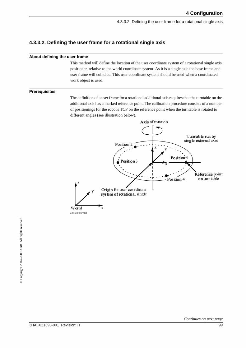
4 Configuration
4.3.3.2. Defining the user frame for a rotational single axis
993HAC021395-001 Revision: H
© C
opyr
ight
200
4-20
09 A
BB
. All
righ
ts r
eser
ved.
4.3.3.2. Defining the user frame for a rotational single axis
About defining the user frame
This method will define the location of the user coordinate system of a rotational single axis
positioner, relative to the world coordinate system. As it is a single axis the base frame and
user frame will coincide. This user coordinate system should be used when a coordinated
work object is used.
Prerequisites
The definition of a user frame for a rotational additional axis requires that the turntable on the
additional axis has a marked reference point. The calibration procedure consists of a number
of positionings for the robot's TCP on the reference point when the turntable is rotated to
different angles (see illustration below).
en0600002760
Continues on next page
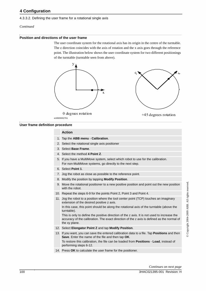
4 Configuration
4.3.3.2. Defining the user frame for a rotational single axis
3HAC021395-001 Revision: H100
© C
opyr
ight
200
4-20
09 A
BB
. All
righ
ts r
eser
ved.
Position and directions of the user frame
The user coordinate system for the rotational axis has its origin in the centre of the turntable.
The z direction coincides with the axis of rotation and the x axis goes through the reference
point. The illustration below shows the user coordinate system for two different positionings
of the turntable (turntable seen from above).
en0600002761
User frame definition procedure
Action
1. Tap the ABB menu - Calibration.
2. Select the rotational single axis positioner
3. Select Base Frame.
4. Select the method 4 Point Z.
5. If you have a MultiMove system, select which robot to use for the calibration.
For non-MultiMove systems, go directly to the next step.
6. Select Point 1.
7. Jog the robot as close as possible to the reference point.
8. Modify the position by tapping Modify Position.
9. Move the rotational positioner to a new positive position and point out the new position with the robot.
10. Repeat the steps 6-9 for the points Point 2, Point 3 and Point 4.
11. Jog the robot to a position where the tool center point (TCP) touches an imaginary extension of the desired positive z axis.
In this case, this point should be along the rotational axis of the turntable (above the turntable).
This is only to define the positive direction of the z axis. It is not used to increase the accuracy of the calibration. The exact direction of the z axis is defined as the normal of the xy plane.
12. Select Elongator Point Z and tap Modify Position.
13. If you want, you can save the entered calibration data to a file. Tap Positions and then Save. Enter the name of the file and then tap OK.
To restore this calibration, the file can be loaded from Positions - Load, instead of performing steps 6-12.
14. Press OK to calculate the user frame for the positioner.
Continued
Continues on next page
4 Configuration
4.3.3.2. Defining the user frame for a rotational single axis
1013HAC021395-001 Revision: H
© C
opyr
ight
200
4-20
09 A
BB
. All
righ
ts r
eser
ved.
Result
The result of the calculation is displayed (expressed in the world coordinate system). The
following values are shown:
If the estimated error is acceptable, press OK to confirm the new user frame.
If the estimated error is unacceptable, press Cancel to redefine the calibration.
Listed values Description
Method Displays the selected calibration method.
Max error The maximum error for one positioning.
Min error The minimum error for one positioning.
Mean error The accuracy of the robot positioning against the tip.
Cartesian X - Z The x, y, z coordinates for the user frame.
Quarternion 1-4 Orientation components for the user frame.
Continued
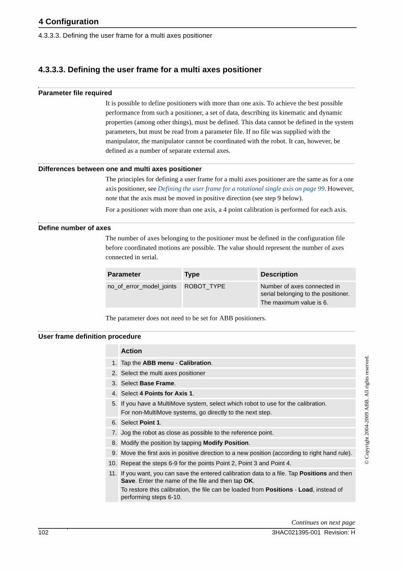
4 Configuration
4.3.3.3. Defining the user frame for a multi axes positioner
3HAC021395-001 Revision: H102
© C
opyr
ight
200
4-20
09 A
BB
. All
righ
ts r
eser
ved.
4.3.3.3. Defining the user frame for a multi axes positioner
Parameter file required
It is possible to define positioners with more than one axis. To achieve the best possible
performance from such a positioner, a set of data, describing its kinematic and dynamic
properties (among other things), must be defined. This data cannot be defined in the system
parameters, but must be read from a parameter file. If no file was supplied with the
manipulator, the manipulator cannot be coordinated with the robot. It can, however, be
defined as a number of separate external axes.
Differences between one and multi axes positioner
The principles for defining a user frame for a multi axes positioner are the same as for a one
axis positioner, see Defining the user frame for a rotational single axis on page 99. However,
note that the axis must be moved in positive direction (see step 9 below).
For a positioner with more than one axis, a 4 point calibration is performed for each axis.
Define number of axes
The number of axes belonging to the positioner must be defined in the configuration file
before coordinated motions are possible. The value should represent the number of axes
connected in serial.
The parameter does not need to be set for ABB positioners.
User frame definition procedure
Parameter Type Description
no_of_error_model_joints ROBOT_TYPE Number of axes connected in serial belonging to the positioner.
The maximum value is 6.
Action
1. Tap the ABB menu - Calibration.
2. Select the multi axes positioner
3. Select Base Frame.
4. Select 4 Points for Axis 1.
5. If you have a MultiMove system, select which robot to use for the calibration.
For non-MultiMove systems, go directly to the next step.
6. Select Point 1.
7. Jog the robot as close as possible to the reference point.
8. Modify the position by tapping Modify Position.
9. Move the first axis in positive direction to a new position (according to right hand rule).
10. Repeat the steps 6-9 for the points Point 2, Point 3 and Point 4.
11. If you want, you can save the entered calibration data to a file. Tap Positions and then Save. Enter the name of the file and then tap OK.
To restore this calibration, the file can be loaded from Positions - Load, instead of performing steps 6-10.
Continues on next page
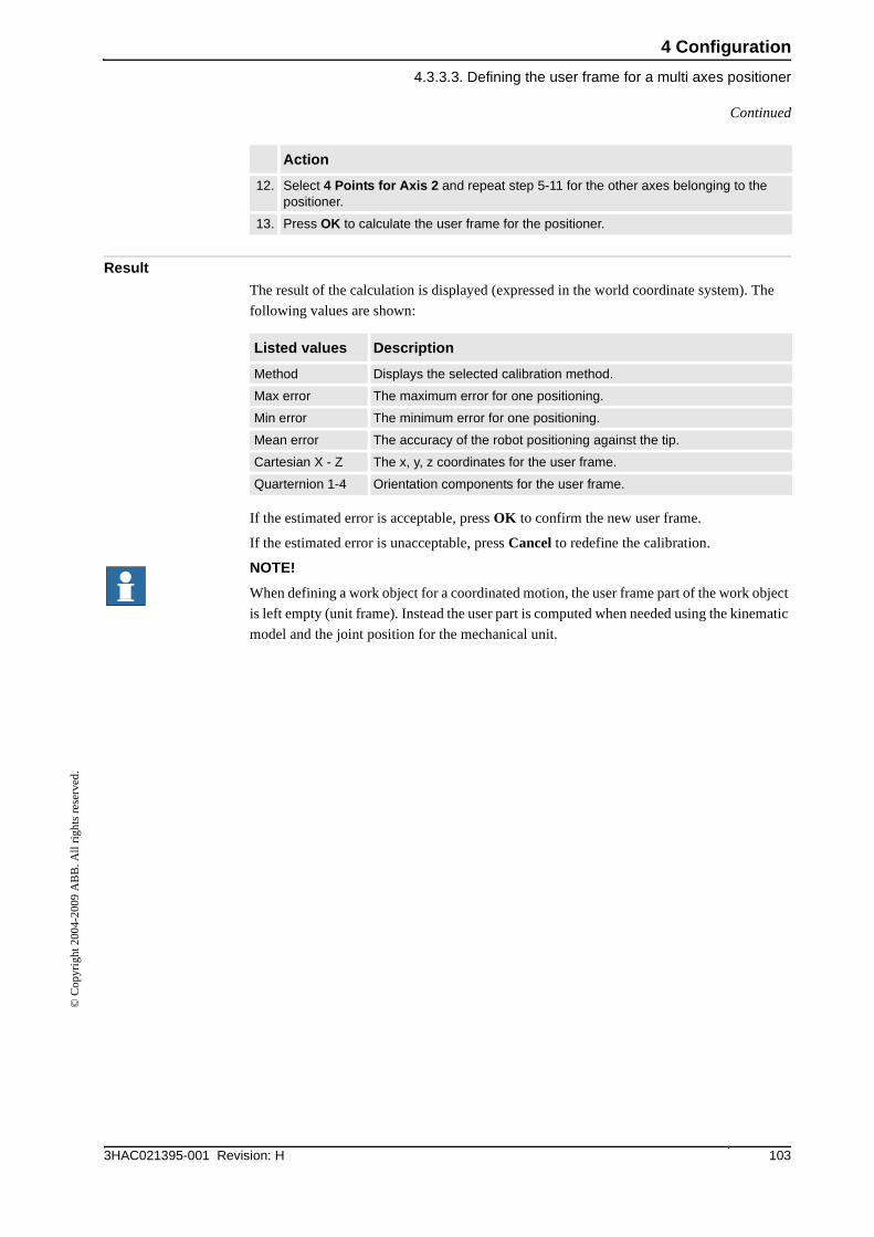
4 Configuration
4.3.3.3. Defining the user frame for a multi axes positioner
1033HAC021395-001 Revision: H
© C
opyr
ight
200
4-20
09 A
BB
. All
righ
ts r
eser
ved.
Result
The result of the calculation is displayed (expressed in the world coordinate system). The
following values are shown:
If the estimated error is acceptable, press OK to confirm the new user frame.
If the estimated error is unacceptable, press Cancel to redefine the calibration.
NOTE!
When defining a work object for a coordinated motion, the user frame part of the work object
is left empty (unit frame). Instead the user part is computed when needed using the kinematic
model and the joint position for the mechanical unit.
12. Select 4 Points for Axis 2 and repeat step 5-11 for the other axes belonging to the positioner.
13. Press OK to calculate the user frame for the positioner.
Action
Listed values Description
Method Displays the selected calibration method.
Max error The maximum error for one positioning.
Min error The minimum error for one positioning.
Mean error The accuracy of the robot positioning against the tip.
Cartesian X - Z The x, y, z coordinates for the user frame.
Quarternion 1-4 Orientation components for the user frame.
Continued

4 Configuration
4.3.3.3. Defining the user frame for a multi axes positioner
3HAC021395-001 Revision: H104
© C
opyr
ight
200
4-20
09 A
BB
. All
righ
ts r
eser
ved.
5 Commutation
5.1. Commutate the motor
1053HAC021395-001 Revision: H
© C
opyr
ight
200
4-20
09 A
BB
. All
righ
ts r
eser
ved.
5 Commutation
5.1. Commutate the motor
Overview
This chapter describes how to use the call service routine commutation, so the additional
motor runs properly.
The service routine commutation is used to:
• Find a commutation value for a synchronous permanent magnet motor.
• Check motor phase order
• Verify the pole pair parameter value is correctly typed in.
• Check resolver connection
How to install a new motor
Set the motor in safe mode/normal mode
The system parameters can be changed in the FlexPendant or in RobotStudio. On the
FlexPendant tap Control panel/Configuration/Topics/Motion/Drive System. Then change the
parameter current_vector_on to TRUE or FALSE in the DRIVE_SYSTEM. If the motor is to
be set in safe mode set the parameter to TRUE or normal mode FALSE.
CAUTION!
If the motor is not properly installed, it can run away and destroy itself or other equipment.
To avoid this set the motor in safe mode.
Action Note
1. Set the motor in safe mode by changing the system parameter current_vector_on to TRUE.
Set the motor in safe mode/normal mode on page 105.
2. Start the service routine Commutation. See Operating manual - IRC5 with FlexPendant section Programming and testing - Running a service routine.
3. Check motor phase order connections. Check motor phase connections order on page 106.
4. Check resolver connection. Check resolver connections on page 106.
5. Move the motor to commutation position.
• For the pre-Commutated motor: Check the motor phase connections.
• For the none commutated motor: Commutate the motor by updating the commutation offset.
Check the motor phase connections on page 106.
Update commutation offset on page 106.
6. The commutation is now finished and the motor is ready to use. When exiting, the program ask if the motor is to be set in normal mode. The motor can also be set to normal mode by changing the parameter current_vector_on to FALSE.
See Set the motor in safe mode/normal mode on page 105.
Continues on next page
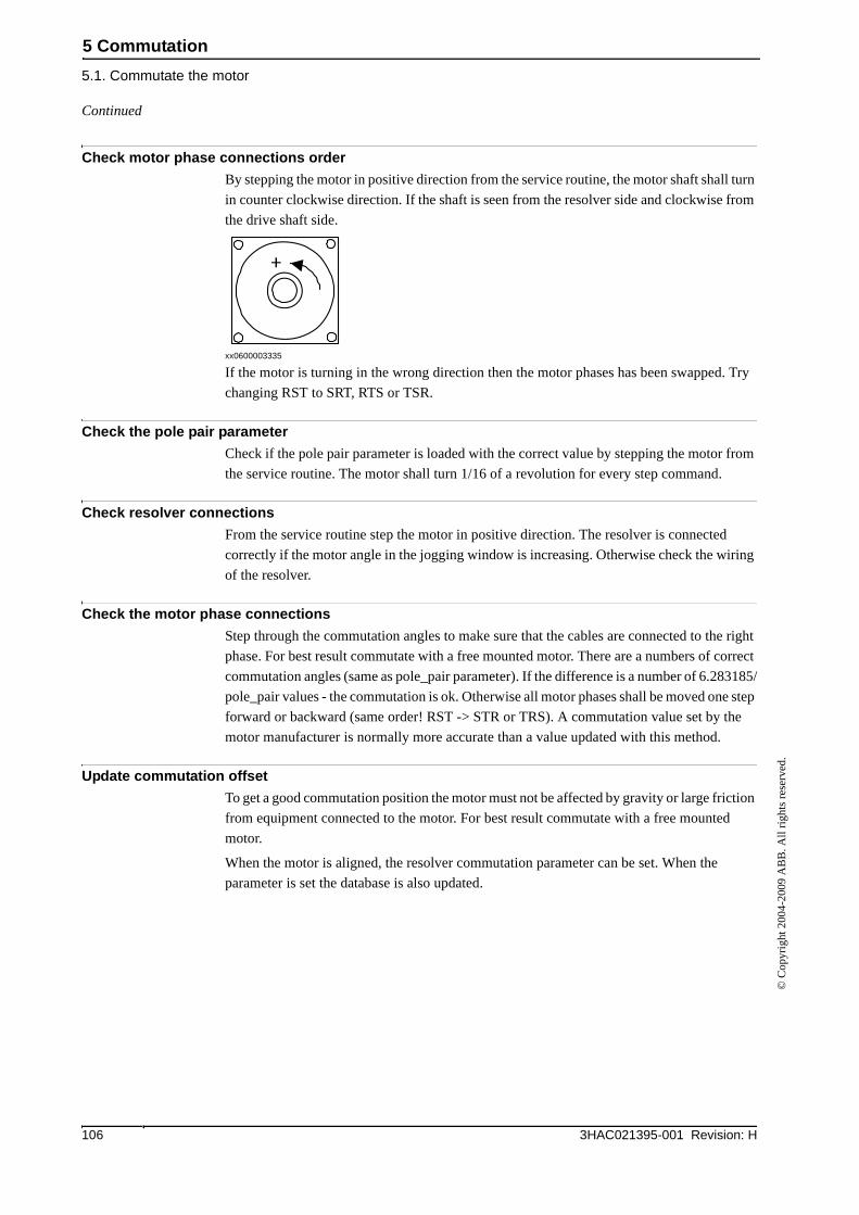
5 Commutation
5.1. Commutate the motor
3HAC021395-001 Revision: H106
© C
opyr
ight
200
4-20
09 A
BB
. All
righ
ts r
eser
ved.
Check motor phase connections order
By stepping the motor in positive direction from the service routine, the motor shaft shall turn
in counter clockwise direction. If the shaft is seen from the resolver side and clockwise from
the drive shaft side.
xx0600003335
If the motor is turning in the wrong direction then the motor phases has been swapped. Try
changing RST to SRT, RTS or TSR.
Check the pole pair parameter
Check if the pole pair parameter is loaded with the correct value by stepping the motor from
the service routine. The motor shall turn 1/16 of a revolution for every step command.
Check resolver connections
From the service routine step the motor in positive direction. The resolver is connected
correctly if the motor angle in the jogging window is increasing. Otherwise check the wiring
of the resolver.
Check the motor phase connections
Step through the commutation angles to make sure that the cables are connected to the right
phase. For best result commutate with a free mounted motor. There are a numbers of correct
commutation angles (same as pole_pair parameter). If the difference is a number of 6.283185/
pole_pair values - the commutation is ok. Otherwise all motor phases shall be moved one step
forward or backward (same order! RST -> STR or TRS). A commutation value set by the
motor manufacturer is normally more accurate than a value updated with this method.
Update commutation offset
To get a good commutation position the motor must not be affected by gravity or large friction
from equipment connected to the motor. For best result commutate with a free mounted
motor.
When the motor is aligned, the resolver commutation parameter can be set. When the
parameter is set the database is also updated.
Continued
6 Tuning
6.1. Tuning the commutation offset
1073HAC021395-001 Revision: H
© C
opyr
ight
200
4-20
09 A
BB
. All
righ
ts r
eser
ved.
6 Tuning
6.1. Tuning the commutation offset
General
Before using an additional axis, you must tune the motors commutation offset. This requires
that you connect a DC power source between two nodes and then measure the position of the
motor.
NOTE!
ABB motors are precommutated with the commutation value 1.5708. Therefore, an ABB
motor does not require tuning of the commutation offset.
Prerequisites
The motor must comply with the specifications in Motors on page 202. The resolver must
comply with the specifications in Resolvers on page 207.
Required materialThis is a list of what you need to perform the tuning:
Measuring procedure
This procedure describes how to measure the commutation position of a motor.
Material Description
PC with Test Signal Viewer The software Test Signal Viewer is delivered on the RobotWare CD.
Power supply 24 V (DC).
The power supply should be equipped with a relay that trips at short circuit. Otherwise a fuse will burn every time the power is applied.
Check the motor data to see the current required from the power supply.
2 cable sets Cables to brake release and motor phase.
Each cable set includes one plus and one minus cable.
Motor documentation Motor data sheet and electrical connection drawing.
Action
1. Deactivate the axis of the motor you want to tune.
2. Switch off the controller.
3. Disconnect the power cable to the motor.
4. Disconnect the motor from the gear (or in some other way make sure the motor is not affected by external torque and friction).
5. If the motor is using a brake, release it by connecting the power supply to the contact pins for the brake release.
See motor specifications for max brake current, which contact are for the brake release and the polarity of the contacts (if any).
6. Ensure that the brake is released by manually turning the motor.
Continues on next page
6 Tuning
6.1. Tuning the commutation offset
3HAC021395-001 Revision: H108
© C
opyr
ight
200
4-20
09 A
BB
. All
righ
ts r
eser
ved.
7. Connect the power supply with the plus cable to the phase S (V) and the minus cable (0 V) to the to the phase T (W).
A short pulse is enough to move the motor to its commutation position. Disconnect the power after the voltage pulse.
8. Connect the power to give another voltage pulse to the motor. If the motor is already in its commutation position it should not move this time.
9. Disconnect the power supply from the brake release, so that the motor brake is on.
10. Reconnect the power cable from the drive module to the motor.
11. Activate the axis.
Do not move any mechanical unit.
12. Start the controller.
13. Configure Test Signal Viewer, selecting mechanical unit and the signal Resolver_angle.
Zoom in on the signal so you can read at least 2 decimals.
Note that the number of commutation positions are equal to the number of pole pairs. E.g. a motor with 2 pole pairs have 2 possible values for this measurement. It does not matter which of the commutation points you are measuring.
14. Set the measured value to the parameter Commutator Offset in the type Motor Calibra-tion.
Action
Continued
6 Tuning
6.2.1. Introduction
1093HAC021395-001 Revision: H
© C
opyr
ight
200
4-20
09 A
BB
. All
righ
ts r
eser
ved.
6.2 Tuning
6.2.1. Introduction
Overview
The servo control parameters can be adjusted (tuned) to achieve the best possible motion
performance.
This section contains a complete description of how to tune the axes and is divided into the
following sections:
• Tuning of axes, complete procedure on page 112 details the complete procedure of
tuning the axes, including necessary preparations and references to more detailed
instructions of setting tuned values for the different parameters.
• Separate procedures that detail how to set the respective tuning parameters.
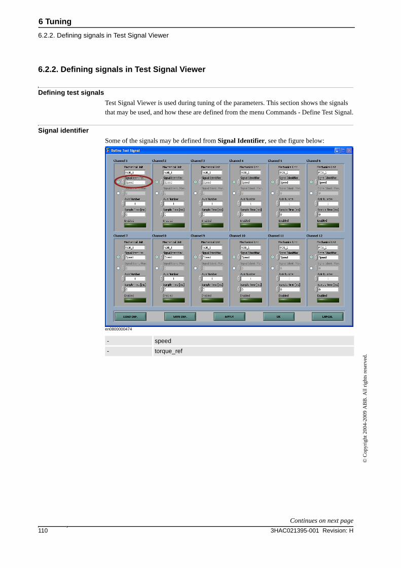
6 Tuning
6.2.2. Defining signals in Test Signal Viewer
3HAC021395-001 Revision: H110
© C
opyr
ight
200
4-20
09 A
BB
. All
righ
ts r
eser
ved.
6.2.2. Defining signals in Test Signal Viewer
Defining test signals
Test Signal Viewer is used during tuning of the parameters. This section shows the signals
that may be used, and how these are defined from the menu Commands - Define Test Signal.
Signal identifier
Some of the signals may be defined from Signal Identifier, see the figure below:
en0800000474
- speed
- torque_ref
Continues on next page
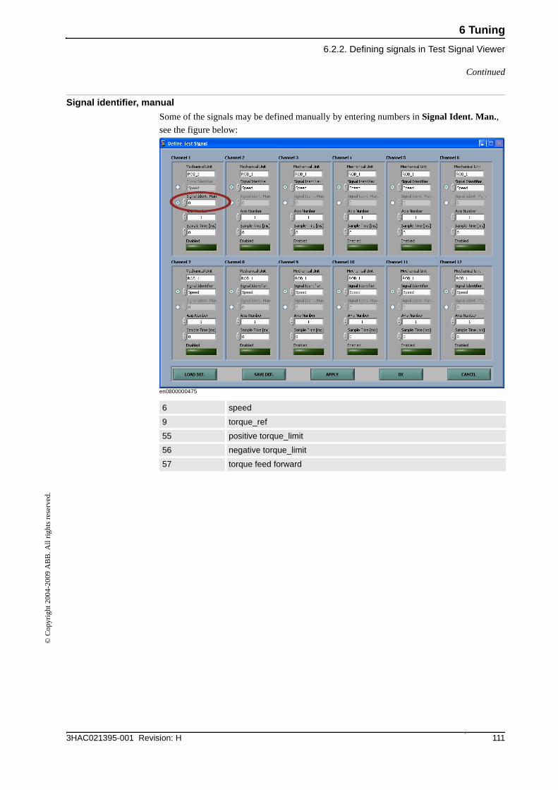
6 Tuning
6.2.2. Defining signals in Test Signal Viewer
1113HAC021395-001 Revision: H
© C
opyr
ight
200
4-20
09 A
BB
. All
righ
ts r
eser
ved.
Signal identifier, manual
Some of the signals may be defined manually by entering numbers in Signal Ident. Man., see the figure below:
en0800000475
6 speed
9 torque_ref
55 positive torque_limit
56 negative torque_limit
57 torque feed forward
Continued
6 Tuning
6.2.3. Tuning of axes, complete procedure
3HAC021395-001 Revision: H112
© C
opyr
ight
200
4-20
09 A
BB
. All
righ
ts r
eser
ved.
6.2.3. Tuning of axes, complete procedure
General
This section details the complete procedure for tuning of the axes, which is done in order to
achieve the best possible motion performance of the robot system.
WARNING!
The system is unstable and therefore dangerous during the tuning process, since bad
parameters or parameter combinations may be used! The safety procedures of the robot
system must be carefully followed throughout the tuning process.
How to set the parameter values
System parameters for tuning are preferably edited by using RobotStudio. They can however
also be edited on the FlexPendant, and even directly in the configuration files by using a text
editor. System parameters are listed in the section System Parameters on page 149. More
information, including parameter names in the configuration files, can be found in Technical
reference manual - System parameters.
Preparations
The following preparations must be made before tuning a servomotor axis:
• Set up the Test Signal Viewer software according to the instructions in the pdf-file
Test Signal Viewer, enclosed with the program.
• Make sure that the additional axis is commutated and calibrated. Any position may be
defined as the calibration position.
• Select or use default tuning parameters so the axis may be jogged without stopping
due to speed or torque supervision.
Tuning calibrated axes, overview
Tuning a calibrated axis means setting values for several parameters in the motion
configuration type Lag Control Master 0. The procedure below is an overview of the
complete tuning procedure and includes references to more detailed instructions of how to
actually set each parameter.
Action
1. Make the Preparations on page 112.
2. Use RobotStudio or the FlexPendant. Select the configuration topic Motion and the type Lag Control Master 0.
3. Set initially tuned values for the parameters Kv, Kp and Ti. This is further detailed in the section Initial tuning of Kv, Kp and Ti on page 115.
Continues on next page
6 Tuning
6.2.3. Tuning of axes, complete procedure
1133HAC021395-001 Revision: H
© C
opyr
ight
200
4-20
09 A
BB
. All
righ
ts r
eser
ved.
4. Set a value for the parameter FFW Mode (feedforward mode) by choosing one of following modes:
• No: This is the easiest configuration with no adjustments of the position lag. (this mode is called 0 in the configuration file)
• Spd: This is the recommended configuration. In this configuration the controller receives information about the desired speed of the axis. As a result, the position lag is considerably reduced compared to the No configuration.
• Trq: In this configuration the controller uses the desired speed and acceleration of the axis to calculate the desired motor torque. This requires knowledge of the mass moment of inertia of the axis, which must be supplied by the user. For this reason this configuration is more difficult to tune, specially for the axes affected by gravity. It is only recommended for experienced users.
The controller is driven by the position lag. This is the offset in time from the point of given command to the point of actual performance of the command. The lag may be adjusted with the different modes in the parameter FFW Mode.
Depending on which mode is chosen for the FFW Mode, further tuning parameters can be set later on.
5. Set a value for the parameter Inertia, depending on the chosen FFW Mode:
• FFW Mode = No: set Inertia to 0
• FFW Mode = Spq: set Inertia to 0
• FFW Mode = Trq: calculate and set Inertia according to the section Specifying the inertia on page 121.
6. If parameter FFW Mode is set to Spd, the following parameters are also available:
• Bandwidth, should be left at its default value
• Delay, should be left at its default value.
7. If parameter FFW Mode is set to Trq, the following parameters are also available:
• Bandwidth, should be left at its default value. Adjustment is detailed in the section Tuning of Bandwidth on page 122.
• Delay, should be left at its default value (0.004). In rare cases, increasing the value may reduce the speed overshot.
• Resonance frequency (flexibility compensation filter), should initially be left at its default value. May be adjusted once the other parameters are set, if the torque_ref signal is oscillatory due to mechanical resonance. How to tune this parameter is detailed in the section Tuning of resonance frequency on page 124.
• Resonance damping (flexibility compensation filter), should be left at its default value (0.01).
8. In the type Acceleration Data, set tuned values for Nominal Acceleration and Nominal Deceleration as detailed in the section Tuning of Nominal Acceleration and Nominal Deceleration on page 125.
9. In Lag Control Master 0, set finally tuned values for the parameters:
• Kv, Gain Speed Loop
• Kp, Gain Position Loop
• Ti Integration Time Speed Loop
This is further detailed in the section Final tuning of Kp, Kv and Ti on page 128.
Action
Continued
Continues on next page
6 Tuning
6.2.3. Tuning of axes, complete procedure
3HAC021395-001 Revision: H114
© C
opyr
ight
200
4-20
09 A
BB
. All
righ
ts r
eser
ved.
Tuning uncalibrated axes, overview
Tuning an uncalibrated axis means setting values for several parameters in the motion
configuration type Uncalibrated Control Master 0. The procedure below is an overview of
the complete tuning procedure and includes references to more detailed instructions of how
to actually set each parameter.
Action
1. Make the Preparations on page 112.
2. Use RobotStudio or the FlexPendant. Select the configuration topic Motion and the type Uncalibrated Control Master 0.
3. Set the initial tuning values of Kv, Gain Speed Loop, Kp, Gain Position Loop, and Ti Integration Time Speed Loop. Use tuned values, set during tuning of a calibrated axis. Use the values so that the axis is movable regardless of the position.
4. Set the tuning value of Speed Max Uncalibrated. Maximum speed for uncalibrated axis (rad/s on motor side).
5. Set the tuning value of Deceleration Max Uncalibrated. Maximum deceleration for uncalibrated axis (rad/s2 on motor side). Recommended value: Nominal Deceleration * Transmission Gear Ratio. How to set the value for the nominal deceleration is detailed in the section Tuning of Nominal Acceleration and Nominal Deceleration on page 125.
6. Set the tuning value of Acceleration Max Uncalibrated. Maximum acceleration for uncal-ibrated axis (rad/s2 on motor side). Recommended value: Nominal Acceleration * Transm Gear Ratio. How to set the value for the nominal acceleration is detailed in the section Tuning of Nominal Acceleration and Nominal Deceleration on page 125.
7. Set the final tuning values of Kv, Gain Speed Loop, Kp, Gain Position Loop, and Ti Integration Time Speed Loop, as detailed in the section Final tuning of Kp, Kv and Ti on page 128.
Continued
6 Tuning
6.2.4. Initial tuning of Kv, Kp and Ti
1153HAC021395-001 Revision: H
© C
opyr
ight
200
4-20
09 A
BB
. All
righ
ts r
eser
ved.
6.2.4. Initial tuning of Kv, Kp and Ti
General
This section details how to make the initial tuning of the parameters Kv, Gain Speed Loop,
Kp, Gain Position Loop and Ti Integration Time Speed Loop.
The general strategy is to tune Kv first while keeping Kp constant and without integral effect
(Ti is set to a high value, e.g. 10), then tune Kp to its maximum value without vibration/
oscillation; finally tune Ti and other parameters.
NOTE!
Check that the additional axes motor file contains the correct motor data.
Parameter description
The parameters Kv, Gain Speed Loop, Kp, Gain Position Loop and Ti Integration Time Speed
Loop belongs to the type Lag Control Master 0 and are further described in the section System
Parameters on page 149.
RAPID program
Program a back-and-forth motion of the axis. For the final tuning of the control parameters
of the axis it is convenient to use the TuneServo command. Each procedure below includes
an example of a RAPID program that can be used.
Initial tuning of Kv
The procedure below details how to make the initial tuning of the parameter Kv, Gain Speed
Loop.
WARNING!
The system is unstable and therefore dangerous during the tuning process, since bad
parameters or parameter combinations may be used! The safety procedures of the robot
system must be carefully followed throughout the tuning process.
Action
1. Set the parameter FFW Mode to No.
2. Make following changes in the type Lag Control Master 0:
• set the value of parameter Kp, Gain Position Loop to 5
• set the value of parameter Ti Integration Time Speed Loop to 10 (a big value in order to eliminate integral portion).
Restart the controller for the changes to take effect.
Continues on next page
6 Tuning
6.2.4. Initial tuning of Kv, Kp and Ti
3HAC021395-001 Revision: H116
© C
opyr
ight
200
4-20
09 A
BB
. All
righ
ts r
eser
ved.
3. Increase the Kv value by 10% in each motion loop, until the axis starts to vibrate/oscillate or a clear vibration can be heard from the axis, either during motion or when stationary. The axis velocity supervision may also indicate speed failure.
The following RAPID program can be used to increase Kv by 10% of the default value set in the loaded configuration file:
MODULE Kv_tune
PROC main()
VAR num i;
VAR num per_Kv;
VAR num Kv;
TuneReset;
FOR i FROM 0 TO 40 DO
per_Kv:=100+10*i;
Kv:=1*per_Kv/100;
TPErase;
TPWrite "per_Kv = "\Num:=per_Kv;
TPWrite "Kv = "\Num:=Kv;
TuneServo STN1,1,100\Type:=TUNE_KP;
TuneServo STN1,1,100\Type:=TUNE_TI;
TuneServo STN1,1,per_Kv\Type:=TUNE_KV;
MoveJ p1,v1000,z50,tool0;
MoveJ p2,v500,z50,tool0;
MoveJ p1,v1000,z50,tool0;
WaitTime 1;
ENDFOR
ENDPROC
ENDMODULE
Note! The velocity data and test positions may be modified depending on the type of robot and axis to be tuned.
The RAPID instructions are described in the Technical reference manual - RAPID Instructions, Functions and Data types.
The Torque_ref signal in the Test Signal Viewer may be used to evaluate the degree of vibration/oscillation. A typical plot of the signal is shown in the figure Illustration, torque_ref plot on page 117.
4. Once an unstable point is reached, divide the current value of Kv by 2.
5. Enter the new value in the parameter Kv, Gain Speed Loop.
Action
Continued
Continues on next page
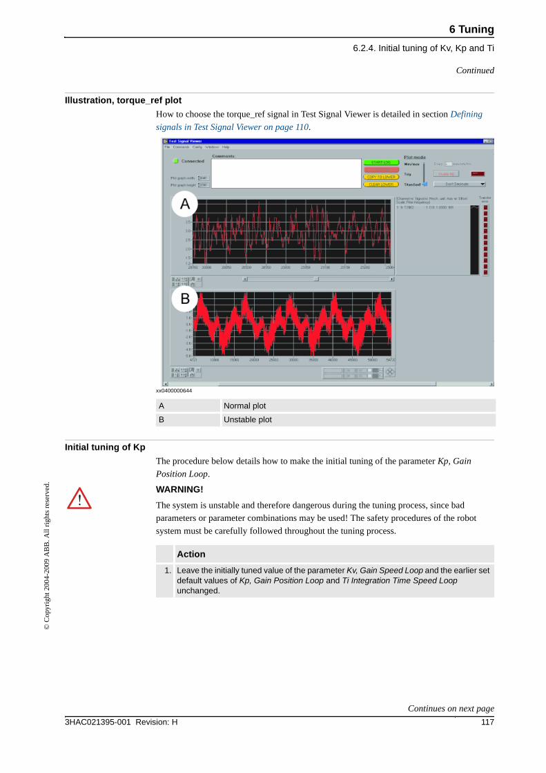
6 Tuning
6.2.4. Initial tuning of Kv, Kp and Ti
1173HAC021395-001 Revision: H
© C
opyr
ight
200
4-20
09 A
BB
. All
righ
ts r
eser
ved.
Illustration, torque_ref plot
How to choose the torque_ref signal in Test Signal Viewer is detailed in section Defining
signals in Test Signal Viewer on page 110.
xx0400000644
Initial tuning of Kp
The procedure below details how to make the initial tuning of the parameter Kp, Gain
Position Loop.
WARNING!
The system is unstable and therefore dangerous during the tuning process, since bad
parameters or parameter combinations may be used! The safety procedures of the robot
system must be carefully followed throughout the tuning process.
A Normal plot
B Unstable plot
Action
1. Leave the initially tuned value of the parameter Kv, Gain Speed Loop and the earlier set default values of Kp, Gain Position Loop and Ti Integration Time Speed Loop unchanged.
Continued
Continues on next page
6 Tuning
6.2.4. Initial tuning of Kv, Kp and Ti
3HAC021395-001 Revision: H118
© C
opyr
ight
200
4-20
09 A
BB
. All
righ
ts r
eser
ved.
2. Increase the Kp value by 10% in each motion loop, until the first signs of overshooting are observed in the velocity plot.
The following RAPID program may be used to increase Kp by 10% of the default value set in the loaded configuration file:
MODULE kp_tune
PROC main()
VAR num i;
VAR num per_Kp;
VAR num Kp;
TuneReset;
FOR i FROM 0 TO 20 DO
per_Kp:=100+10*i;
Kp:=5*per_Kp/100;
TPErase;
TPWrite "per_Kp = "\Num:=per_Kp;
TPWrite "Kp = "\Num:=Kp;
TuneServo STN1,1,100\Type:=TUNE_KV;
TuneServo STN1,1,100\Type:=TUNE_TI;
TuneServo STN1,1,per_Kp\Type:=TUNE_KP;
MoveJ p1,v1000,z50,tool0;
MoveJ p2,v500,z50,tool0;
MoveJ p1,v1000,z50,tool0;
WaitTime 1;
ENDFOR
ENDPROC
ENDMODULE
Note! The velocity data and test positions may be modified depending on the type of robot and axis to be tuned.
The RAPID instructions are described in the Technical reference manual - RAPID Instructions, Functions and Data types.
A typical plot with speed overshot in Test Signal Viewer is shown in the figure Illustration, speed plot on page 119.
3. Once an overshot is observed, subtract 1 from the current value of Kp.
If an overshooting is observed at a later time, the Kp must be reduced to an even lower value.
4. Enter this new value in the parameter Kp, Gain Position Loop.
Action
Continued
Continues on next page
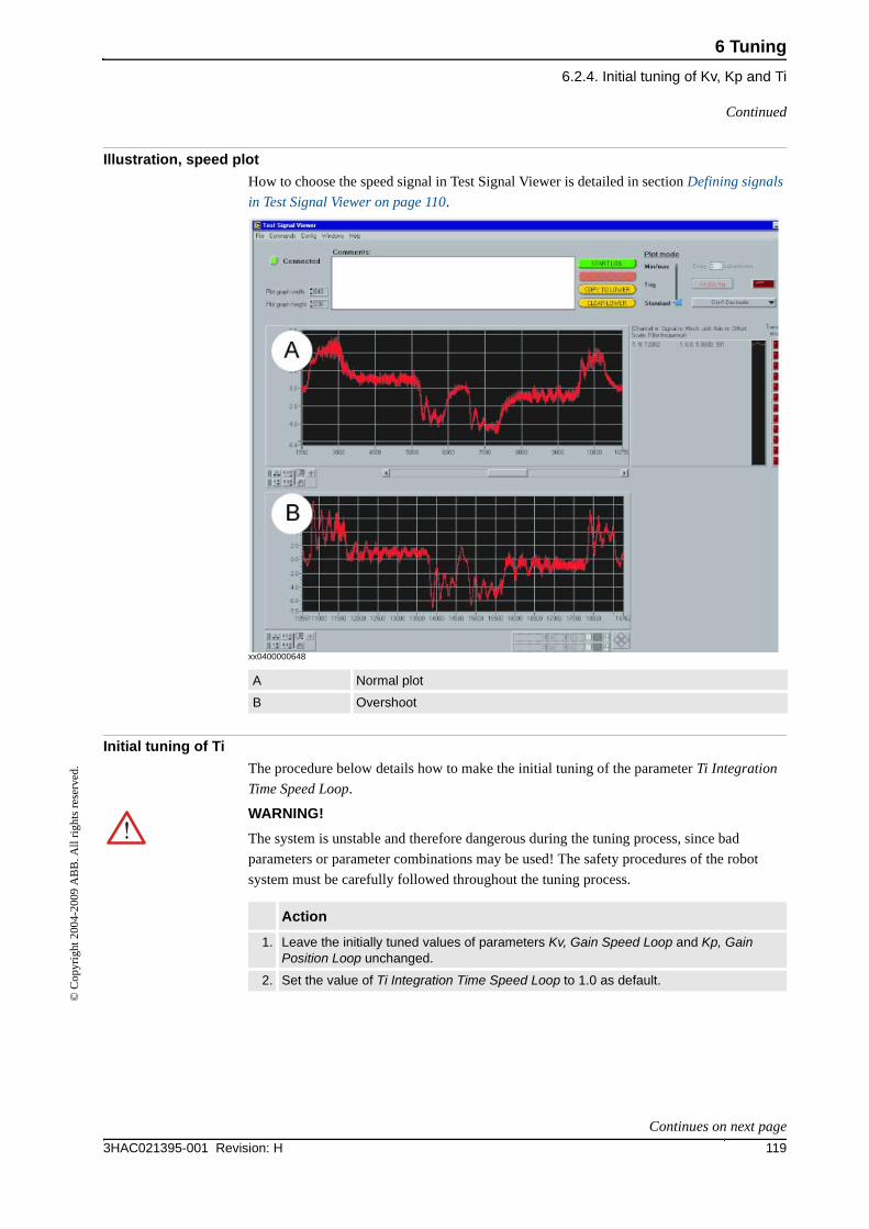
6 Tuning
6.2.4. Initial tuning of Kv, Kp and Ti
1193HAC021395-001 Revision: H
© C
opyr
ight
200
4-20
09 A
BB
. All
righ
ts r
eser
ved.
Illustration, speed plot
How to choose the speed signal in Test Signal Viewer is detailed in section Defining signals
in Test Signal Viewer on page 110.
xx0400000648
Initial tuning of Ti
The procedure below details how to make the initial tuning of the parameter Ti Integration
Time Speed Loop.
WARNING!
The system is unstable and therefore dangerous during the tuning process, since bad
parameters or parameter combinations may be used! The safety procedures of the robot
system must be carefully followed throughout the tuning process.
A Normal plot
B Overshoot
Action
1. Leave the initially tuned values of parameters Kv, Gain Speed Loop and Kp, Gain Position Loop unchanged.
2. Set the value of Ti Integration Time Speed Loop to 1.0 as default.
Continued
Continues on next page
6 Tuning
6.2.4. Initial tuning of Kv, Kp and Ti
3HAC021395-001 Revision: H120
© C
opyr
ight
200
4-20
09 A
BB
. All
righ
ts r
eser
ved.
Result
The parameters Kv, Gain Speed Loop, Kp, Gain Position Loop and Ti Integration Time Speed
Loop are now initially tuned. Continue with the tuning process as described in next section.
The complete tuning procedure is detailed in section Tuning of axes, complete procedure on
page 112.
3. Reduce the Ti value by 10% in each motion loop, until an overshot is observed on the velocity profile in Test Signal Viewer.
Looking at the torque_ref signal can also help to determine the critical value of Ti.
The following RAPID program may be used to reduce the Ti value by 10% of the default value set in the loaded configuration file:
MODULE ti_tune
PROC main()
VAR num i;
VAR num per_Ti;
VAR num Ti;
TuneReset;
FOR i FROM 0 TO 10 DO
per_Ti:=100-10*i;
Ti:=1*per_Ti/100;
TPErase;
TPWrite "per_Ti = "\Num:=per_Ti;
TPWrite "Ti = "\Num:=Ti;
TuneServo STN1,1,200\Type:=TUNE_KV;
TuneServo STN1,1,250\Type:=TUNE_KP;
TuneServo STN1,1,per_Ti\Type:=TUNE_TI;
MoveJ p1,v1000,z50,tool0;
MoveJ p2,v500,z50,tool0;
MoveJ p1,v1000,z50,tool0;
WaitTime 1;
ENDFOR
ENDPROC
ENDMODULE
Note! The velocity data and test positions may be modified depending on the type of robot and axis to be tuned.
The RAPID instructions are described in the Technical reference manual - RAPID Instructions, Functions and Data types.
4. Once an overshot is observed, stop reducing and instead increase the tuned value by 5-10%, in order to remove the effect.
5. When the effect is removed, enter the new value in Ti Integration Time Speed Loop.
Action
Continued
6 Tuning
6.2.5. Specifying the inertia
1213HAC021395-001 Revision: H
© C
opyr
ight
200
4-20
09 A
BB
. All
righ
ts r
eser
ved.
6.2.5. Specifying the inertia
General
This section details how to specify the mass moment of inertia. (only recommended for
experienced users).
Prerequisite
The parameter FFW Mode (in the type Lag Control Master 0) must be set to Trq, in order to
have use of Inertia. If FFW Mode is set to No or Spd, the parameter Inertia is not used, but
should be set to 0 anyway.
Specifying the inertia
The procedure below details how to calculate the mass moment of inertia and how to enter
this value.
Result
The parameter Inertia is now tuned. Continue with the tuning procedure.
Action
1. The inertia is given by:
Inertia = Inertiaaxis / (Transm gear ratio)2 + Inertiamotor + Inertia brake
2. Enter this value for the parameter Inertia in the type Lag Control Master 0.
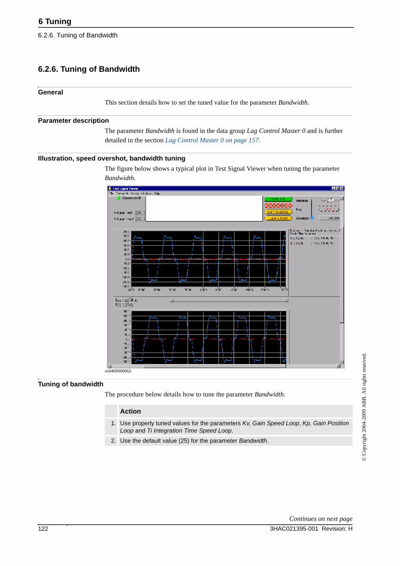
6 Tuning
6.2.6. Tuning of Bandwidth
3HAC021395-001 Revision: H122
© C
opyr
ight
200
4-20
09 A
BB
. All
righ
ts r
eser
ved.
6.2.6. Tuning of Bandwidth
General
This section details how to set the tuned value for the parameter Bandwidth.
Parameter description
The parameter Bandwidth is found in the data group Lag Control Master 0 and is further
detailed in the section Lag Control Master 0 on page 157.
Illustration, speed overshot, bandwidth tuning
The figure below shows a typical plot in Test Signal Viewer when tuning the parameter
Bandwidth.
xx0400000652
Tuning of bandwidth
The procedure below details how to tune the parameter Bandwidth.
Action
1. Use properly tuned values for the parameters Kv, Gain Speed Loop, Kp, Gain Position Loop and Ti Integration Time Speed Loop.
2. Use the default value (25) for the parameter Bandwidth.
Continues on next page
6 Tuning
6.2.6. Tuning of Bandwidth
1233HAC021395-001 Revision: H
© C
opyr
ight
200
4-20
09 A
BB
. All
righ
ts r
eser
ved.
Result
The parameter Bandwidth is now initially tuned. Continue with the tuning process described
in the next section, and in section Tuning of axes, complete procedure on page 112.
3. In order to verify and tune the default Bandwidth value, run a motion program to see if the speed overshot occurs. If the overshoot is out of the tolerance, reduce the value of Bandwidth under the system resonance frequency.
The system resonance frequency may not always be identified. Therefore the value may be varying several times and it may be necessary to perform a check of the speed overshoot and of the following error between command position and actual position. Normally, the bigger the Bandwidth value, the smaller the following error.
A typical speed overshoot plot is shown in the figure Illustration, speed overshot, bandwidth tuning on page 122.
Action
Continued
6 Tuning
6.2.7. Tuning of resonance frequency
3HAC021395-001 Revision: H124
© C
opyr
ight
200
4-20
09 A
BB
. All
righ
ts r
eser
ved.
6.2.7. Tuning of resonance frequency
General
This section details how to set the value of the system parameter Df (resonance frequency).
Parameter description
The parameter Df is found in the type Lag Control Master 0 and is further detailed in the
section Lag Control Master 0 on page 157.
Tuning of resonance frequency
The procedure below details how to tune the resonance frequency.
WARNING!
The system is unstable and therefore dangerous during the tuning process, since bad
parameters or parameter combinations may be used! The safety procedures of the robot
system must be carefully followed throughout the tuning process.
Result
The parameter Df is now tuned. Continue with the tuning procedure as described in the next
section, and in section Tuning of axes, complete procedure on page 112.
Action
1. Measure the distance between the resonance peaks (in points) on the plot of the torque_ref signal. Divide the sampling frequency with this value:
resonance frequency = sampling frequency / distance between resonance peaks
This calculation gives a rough estimate (in 1/s).
Note! The sampling frequency of the logged data depends on the sampling interval that has been selected in the configuration of Test Signal Viewer.
2. The value of the resonance frequency should be in the range 3 to 25 (default 100). To tune the resonance frequency, program a short back-and-forth motion of the axis at maximum speed. The axis should not be allowed to reach full speed before decelera-tion. Use the TUNE_DF argument of the TuneServo command to adjust the resonance frequency and examine the torque_ref signal.
Adjust the resonance frequency until the oscillations in the torque_ref signal are damped out.
3. Enter the tuned value of the resonance frequency to the parameter Df.
6 Tuning
6.2.8. Tuning of Nominal Acceleration and Nominal Deceleration
1253HAC021395-001 Revision: H
© C
opyr
ight
200
4-20
09 A
BB
. All
righ
ts r
eser
ved.
6.2.8. Tuning of Nominal Acceleration and Nominal Deceleration
General
This section details how to tune the parameters Nominal Acceleration and Nominal
Deceleration.
Parameter description
The parameters Nominal Acceleration and Nominal Deceleration belongs to the type
Acceleration Data and are further described in the section Acceleration Data on page 149.
Preparations
The following preparations must be made before performing the tuning:
If an axis has a varying moment of inertia, Nominal Accelerationand Nominal
Deceleration should be tuned with the maximum moment of inertia. For a description of
how to specify the inertia see Specifying the inertia on page 121.
If gravity has an influence on the axis, then Nominal Acceleration should be tuned with a
motion accelerating upwards gravity. Nominal Deceleration should be tuned with a
stopping motion (deceleration) while moving downwards in gravity direction.
Program two test points for acceleration and two test points for deceleration with the
following requirements:
• Velocity: choose a velocity that is approximately 50% of the maximum speed of the
additional axis.
• Distance: the distance should be chosen to ensure that the axis stabilizes at the
programmed velocity before deceleration starts.
Continues on next page
6 Tuning
6.2.8. Tuning of Nominal Acceleration and Nominal Deceleration
3HAC021395-001 Revision: H126
© C
opyr
ight
200
4-20
09 A
BB
. All
righ
ts r
eser
ved.
Tuning of Nominal Acceleration and Nominal Deceleration
The procedure below details how to tune the parameters Nominal Acceleration and Nominal
Deceleration.
Before beginning the tuning, observe the following warnings:
WARNING!
The system is unstable and therefore dangerous during the tuning process, since bad
parameters or parameter combinations may be used! The safety procedures of the robot
system must be carefully followed throughout the tuning process.
WARNING!
Kp can affect the torque level (torque_ref). Therefore, acceleration/deceleration tuning
should be verified again if Kp is changed more than 10%.
WARNING!
For low values of Kp (e.g. <5) the axis might never reach the acceleration/deceleration value
and these values can be tuned to unrealistically high values without reaching the torque limit.
This can cause problems during an emergency stop if brake_control_on_delay is >0 (motors
used at emergency stop). Do not continue to increase acceleration/deceleration if the effect
on torque_ref is small. Always verify torque_ref level at emergency stop.
Action Note
1. Use Test Signal Viewer software to record the values of positive/negative torque_limit and torque_ref for the axis.
How to define these signals is detailed in section Defining signals in Test Signal Viewer on page 110.
2. Use test positions for Nominal Acceleration and do the following:
1. Run the motion and check the value of torque_ref for the positive/negative torque_limit.
2. Adjust the value of Nominal Acceleration upwards or downwards in increments of 0.5 until the torque_ref signal shows that the axis approaches, but does not reach, the torque limit.
3. Reduce the final value by 10% to allow for variations in the mechanical system over a period of time.
3. Use test positions for Nominal Deceleration and do the following:
1. Run the motion and check the value of torque_ref for the positive/negative torque_limit.
2. Adjust the value of Nominal Deceleration upwards or downwards in increments of 0.5 until the torque_ref signal shows that the axis approaches, but does not reach, the torque limit.
3. Reduce the final value by 10% to allow for variations in the mechanical system over a period of time.
Continued
Continues on next page
6 Tuning
6.2.8. Tuning of Nominal Acceleration and Nominal Deceleration
1273HAC021395-001 Revision: H
© C
opyr
ight
200
4-20
09 A
BB
. All
righ
ts r
eser
ved.
Result
The parameters Nominal Acceleration and Nominal Deceleration are now tuned. Continue
with the tuning process as described in the next section. The complete tuning procedure is
detailed in section Tuning of axes, complete procedure on page 112.
Continued
6 Tuning
6.2.9. Final tuning of Kp, Kv and Ti
3HAC021395-001 Revision: H128
© C
opyr
ight
200
4-20
09 A
BB
. All
righ
ts r
eser
ved.
6.2.9. Final tuning of Kp, Kv and Ti
General
This section details how to tune the parameters Kv, Gain Speed Loop, Kp, Gain Position Loop
and Ti Integration Time Speed Loop.
Parameter description
The parameters Kv, Gain Speed Loop, Kp, Gain Position Loop and Ti Integration Time Speed
Loop belongs to the type Lag Control Master 0 and are further described in the section System
Parameters on page 149.
Preparations
The following preparations must be made before performing the final tuning:
The parameters must be initially tuned as detailed in the section Initial tuning of Kv, Kp
and Ti on page 115.
If the axis has a varying moment of inertia, Kv, Kp and Ti should be tuned with the
maximum value for the moment of inertia.
Program two test points with the following requirements:
• Velocity: choose a velocity that is approximately 25% of the maximum speed of the
additional axis. The speed must be low enough to guarantee that the axis does not
encounter the torque limit but high enough to prevent friction from affecting the result.
• Distance: choose a distance that ensures that the axis stabilizes at the programmed
velocity before deceleration starts.
RAPID program
The following RAPID program can be used during the final tuning of the parameters Kv, Gain
Speed Loop, Kp, Gain Position Loop, and Ti Integration Time Speed Loop:
PROC main()
ActUnit STN1;
TuneServo STN1,1,TuneValue\Type:=TUNE_KP;
TuneServo STN1,1,TuneValue\Type:=TUNE_KV;
TuneServo STN1,1,TuneValue\Type:=TUNE_TI;
FOR i FROM 1 TO 10 DO
MoveJ p1,v_tune,fine,tool0;
MoveJ p2,v_tune,fine,tool0;
MoveJ p1,v_tune,fine,tool0;
ENDFOR
DeactUnit STN1;
ENDPROC
The argument TuneValue is a percentage (1-500) of the set value in the loaded configuration
file. 100% is the normal value.
Further descriptions of the RAPID instructions and arguments are found in Technical
reference manual - RAPID Instructions, Functions and Data types.
Continues on next page
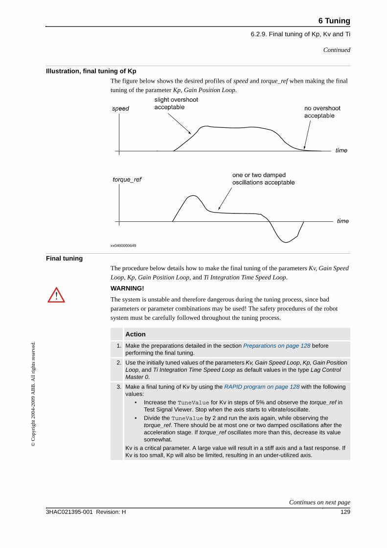
6 Tuning
6.2.9. Final tuning of Kp, Kv and Ti
1293HAC021395-001 Revision: H
© C
opyr
ight
200
4-20
09 A
BB
. All
righ
ts r
eser
ved.
Illustration, final tuning of Kp
The figure below shows the desired profiles of speed and torque_ref when making the final
tuning of the parameter Kp, Gain Position Loop.
xx0400000649
Final tuning
The procedure below details how to make the final tuning of the parameters Kv, Gain Speed
Loop, Kp, Gain Position Loop, and Ti Integration Time Speed Loop.
WARNING!
The system is unstable and therefore dangerous during the tuning process, since bad
parameters or parameter combinations may be used! The safety procedures of the robot
system must be carefully followed throughout the tuning process.
Action
1. Make the preparations detailed in the section Preparations on page 128 before performing the final tuning.
2. Use the initially tuned values of the parameters Kv, Gain Speed Loop, Kp, Gain Position Loop, and Ti Integration Time Speed Loop as default values in the type Lag Control Master 0.
3. Make a final tuning of Kv by using the RAPID program on page 128 with the following values:
• Increase the TuneValue for Kv in steps of 5% and observe the torque_ref in Test Signal Viewer. Stop when the axis starts to vibrate/oscillate.
• Divide the TuneValue by 2 and run the axis again, while observing the torque_ref. There should be at most one or two damped oscillations after the acceleration stage. If torque_ref oscillates more than this, decrease its value somewhat.
Kv is a critical parameter. A large value will result in a stiff axis and a fast response. If Kv is too small, Kp will also be limited, resulting in an under-utilized axis.
Continued
Continues on next page
6 Tuning
6.2.9. Final tuning of Kp, Kv and Ti
3HAC021395-001 Revision: H130
© C
opyr
ight
200
4-20
09 A
BB
. All
righ
ts r
eser
ved.
Result
The parameters Kv, Gain Speed Loop, Kp, Gain Position Loop, and Ti Integration Time Speed
Loop are now finally tuned.
4. Make a final tuning of Kp by using the RAPID program on page 128 and the following information:
• Increase the TuneValue for Kp slowly until the desired speed and torque_ref profiles are achieved as shown in the figure Illustration, final tuning of Kp on page 129. The position error (lag) is inversely proportional to Kp thus a large value for Kp is desirable.
5. Make a final tuning of Ti by using the RAPID program on page 128 with the following values:
• Reduce the TuneValue for Ti in steps of 5% until the effect can be seen on the plot of speed as an increased overshoot.
• Increase the TuneValue for Ti by 5-10% until the effect is removed.
6. Calculate the final values of Kv, Kp and Ti by multiplying the initially tuned value in the configuration file (that was used as the default value) by the given TuneValue divided by 100.
Default value * (TuneValue / 100)
7. Enter these new values to the parameters Kv, Gain Speed Loop, Kp, Gain Position Loop and Ti Integration Time Speed Loop in the type Lag Control Master 0.
Action
Continued
6 Tuning
6.2.10. Tuning of the soft servo parameters
1313HAC021395-001 Revision: H
© C
opyr
ight
200
4-20
09 A
BB
. All
righ
ts r
eser
ved.
6.2.10. Tuning of the soft servo parameters
General
This section details how to tune the following parameters in the type Lag Control Master 0:
• K Soft Min Factor
• K Soft Max Factor
• Kp/Kv Ratio Factor
• Ramp Time
TIP!
In most applications these parameters do not have to be trimmed and can be left at their
default values.
Tuning of K Soft Min Factor
The procedure below details how to make the initial tuning of the parameter K Soft Min
Factor.
TIP!
The movements in this trim procedure should be done close to the point where the soft servo
is activated, to minimize the risk of an axis collapsing.
Tuning of K Soft Max Factor
In most cases, K Soft Max Factor can be left at its default value (1.0).
If the axis is too stiff at 0% softness, reduce K Soft Max Factor. If the axis is too soft at 0%
softness, increase K Soft Max Factor. The tuning can be made in a similar way as for K Soft
Min Factor, but with smaller movements.
Kp/Kv Ratio Factor
Kp/Kv Ratio Factor determines the stability margin for the axis. A value less than 1.0
increases the stability. It is not possible to set this parameter to a value larger than 1.0 since
the stability of the axis would be jeopardized.
Ramp Time
If Ramp Time is changed, the duration of the activation and deactivation phase will change.
A short ramp time can result in a twitch of the axis at activation.
Action
1. Determine a maximum axis movement for which the axis should not move, when the softness is 100%. Such a movement can be 0.1 rad for a rotating axis.
2. Determine a minimum axis movement for which the axis should move, when the softness is 100%. Such a movement can be 0.2 rad for a rotating axis.
3. Activate the soft servo with softness 100% and perform the two movements.
4. If the axis moves for both movements, the axis is too stiff and K Soft Min Factor should be reduced. If the axis does not move for any movement, the axis is too soft and K Soft Min Factor should be increased.
5. Repeat step 3 and 4 until the axis does not move for the smaller movement but does move for the bigger movement.
6 Tuning
6.3.1. Introduction
3HAC021395-001 Revision: H132
© C
opyr
ight
200
4-20
09 A
BB
. All
righ
ts r
eser
ved.
6.3 Additional tuning for servo guns
6.3.1. Introduction
About tuning of servo guns
For a servo gun there are some additional parameters that need tuning. These parameters
belong to types Force Master and Force Master Control.
NOTE!
This tuning must be done before setting up the torque/ force table described in Tip force on
page 74.
TIP!
To simplify the tuning the STTune instruction should be used.
About the STTune instruction
The STTune instruction is a RAPID instruction used to modify parameter values without
having to do a warm start. The argument of the instruction specifies which parameter should
be tuned and the new parameter value. For more information about STTune, see Technical
reference manual - RAPID Instructions, Functions and Data types.
Example
This instruction will tune the parameter Ramp when Increasing Force to the value 100 Nm/s.
STTune M7C1B1_S, 100, RampTorqRefClose;
Parameter argument
Below is a list of the values of the parameter argument used in this chapter, and which system
parameters they correlate to:
Argument values in STTune System parameter name
RampTorqRefClose Ramp when Increasing Force or Ramp Time
KV Kv1 to Kv6
SpeedLimit Speed Limit 1 to Speed Limit 6
CollAlarmTorq Collision Alarm Torque
CollContactPos Collision Delta Position (m)
CollisionSpeed Collision Speed (m/s)
SyncCheckOff Sync check off
6 Tuning
6.3.2. Protecting the gun
1333HAC021395-001 Revision: H
© C
opyr
ight
200
4-20
09 A
BB
. All
righ
ts r
eser
ved.
6.3.2. Protecting the gun
General
To protect the gun from too high forces two system parameters should be set. They are:
• Torque Absolute Max, belonging to the type Stress Duty Cycle
• Max Force Control Motor Torque, belonging to the type SG Process
Prerequisites
To set these values one needs to know maximum allowed motor torque for the motor and
maximum allowed tip force, specified by the gun manufacturer. Some sort of force sensor is
also needed.
Preparations
Before starting, make sure that the gun is calibrated. Jog the tips to contact and calibrate the
axis.
Perform a service calibration (from the program editor on the FlexPendant, tap on Debug,
then Call Service Rou. and select ManServiceCalib).
If you are using the option Servo Tool Control, you need to set the parameter Sync check off
(this is done automatically by the ManServiceCalib if you have the option Spot Servo).
Setting Sync check off will allow you to close the gun without having performed a tip
calibration. To temporarily set Sync check off, use the STTune instruction:
STTune M7C1B1_S, 1, SyncCheckOff;
If error38104: Overspeed during teach mode, appears during the calibration increase the
value of the configuration parameter teach_mode_speed_max_dsp. Change the value in the
servo gun configuration file under SUPERVISION_TYPE. The parameter is not visible from
FlexPendant or RobotStudio.
Initial value is 0.28. Increase to about 0.45.
RAPID program
Create a RAPID program containing the STClose instruction. The argument TipForce
should be set to 1N and Thickness set to the thickness of the force sensor.
tip_force:=1;
STClose M7C1B1_S, tip_force, sensor_thickness;
WaitTime 1;
STOpen M7C1B1_S;
TIP!
If you have any of the RobotWare Spot options, you can replace the three instructions
STClose, WaitTime, and STOpen with the instruction SetForce.
Continues on next page
6 Tuning
6.3.2. Protecting the gun
3HAC021395-001 Revision: H134
© C
opyr
ight
200
4-20
09 A
BB
. All
righ
ts r
eser
ved.
Procedure
This procedure describes how to tune the parameters Torque Absolute Max and Max Force
Control Motor Torque, used to protect the gun from too high forces.
Action
1. Start by setting the force-torque relationship to unity (See Tip force on page 74). Ordered force 1N should give a motor torque of 1 Nm. Note that if the gear ratio, in the type Transmission, is positive the torque values should be negative.
It is enough to define 2 force-torque relationships. In the type SG Process, set Number of Stored Forces to 2, Tip Force 1 to 1, Tip Force 2 to 2, Motor Torque 1 to 1 and Motor Torque 2 to 2 if gear ratio is negative (-1 and -2 if gear ratio is positive).
2. In the type Stress Duty Cycle, set Torque Absolute Max to the value found in the motor specifications.
3. Make a warm start of the controller for the new parameter values to take effect.
4. Execute the program and record the tip force. Increase the ordered tip force while measuring the actual tip force until the actual tip force is close to the specified maximum tip force. For future use also find a torque value corresponding to a typical tip force used during welding.
5. Because the force-torque relation was set to unity the value in forcedata giving maximum allowed tip force corresponds to the maximum allowed motor torque. Set the values of Torque Absolute Max and Max Force Control Motor Torque to this value.
The new value of Torque Absolute Max may be a reduction from the value found earlier (see previous chapters). If that is the case, the values of Nominal Acceleration and Nominal Deceleration (in the type Acceleration Data) may have to be lowered because the torque available for acceleration has decreased.
Continued
6 Tuning
6.3.3. Position Interpolation
1353HAC021395-001 Revision: H
© C
opyr
ight
200
4-20
09 A
BB
. All
righ
ts r
eser
ved.
6.3.3. Position Interpolation
About References Bandwidth
The parameter References Bandwidth belongs to the type Force Master and decides the
bandwidth of the position references generated to reach the contact position before switching
to force control.
Procedure
Leave References Bandwidth at its default value (25Hz). If there are some problems with
oscillations in torque or speed the bandwidth may be reduced.
6 Tuning
6.3.4. Tuning ramp times for force ramping
3HAC021395-001 Revision: H136
© C
opyr
ight
200
4-20
09 A
BB
. All
righ
ts r
eser
ved.
6.3.4. Tuning ramp times for force ramping
Two ways to configure the ramp
There are two different ways to configure how fast the force is increased to its ordered value.
The first method is by deciding how fast the motor torque should increase per second. The
corresponding parameter that needs tuning is Ramp when Increasing Force. The second
method is by specifying how long time the ramp should take. This approach means that the
ramping will be steeper for high forces, something that increases the linearity between force
and torque and thereby reduces the calibration effort. The corresponding parameter in this
case is Ramp Time. To choose between these two approaches a parameter, Use Ramp Time, is
used. By setting this parameter to TRUE the second method is used.
Prerequisites
Depending on the type of gun, different parameter values might be optimal. For tuning of the
parameters, a force sensor that can read the force during the whole closing procedure would
be optimal. If that is not available, use Test Signal Viewer and log position (Signal no. 18),
motor speed (speed) and motor torque (torque_ref).
RAPID program
Make a RAPID program containing a STClose instruction with ordered force chosen so the
tip force will be a force typically used. The program should also include a STTune instruction
with the argument value RampTorqRefClose. If the parameter Use Ramp Time is set to
TRUE this tune instruction modifies the value of Ramp Time else it modifies Ramp when
Increasing Force.
In case Use Ramp Time is set to FALSE the program may look like the one below. To be sure
that the speed limitation does not affect the result, include a tune instruction setting the speed
limit to a high value.
STTune M7C1B1_S, 200, SpeedLimit;
FOR i FROM 20 TO 220 STEP 40
STTune M7C1B1_S, i, RampTorqRefClose;
STClose M7C1B1_S, tip_force, thickness;
WaitTime 1;
STOpen M7C1B1_S;
ENDFOR
STTuneReset M7C1B1_S;
In case Use ramp time is set to TRUE the values tested should be in milliseconds. A
reasonable choice is to modify the FOR loop as below:
FOR i FROM 0.020 TO 0.100 STEP 0.01
TIP!
If you have any of the RobotWare Spot options, you can replace the three instructions
STClose, WaitTime and STOpen with the instruction SetForce.
Continues on next page
6 Tuning
6.3.4. Tuning ramp times for force ramping
1373HAC021395-001 Revision: H
© C
opyr
ight
200
4-20
09 A
BB
. All
righ
ts r
eser
ved.
Procedure
This procedure describes how to tune the force ramping. What we want is to have as fast rise
time as possible without getting any other unwanted effects like overshoot in the force. A
large overshoot in the force signal is usually also seen in the position and the speed signals.
Make sure the calibration of the gun and ordered contact position is correct. Incorrect
calibration will usually show as an overshoot of the force signal.
Action
1. Run the RAPID program shown above.
2. If a force sensor is available, look at the overshoot of the force signal. Choose a ramp value that does not give a large overshoot.
3. After deciding a value of Ramp when Increasing Force or Ramp Time, let the RAPID program run in continuous mode for a while and study the test signals to make sure that no unexpected effects show.
Continued
6 Tuning
6.3.5. Speed versus force repeatability
3HAC021395-001 Revision: H138
© C
opyr
ight
200
4-20
09 A
BB
. All
righ
ts r
eser
ved.
6.3.5. Speed versus force repeatability
Delay Ramp
Quite often there is a trade-off between short cycle times and good force repeatability. To get
better force repeatability there is a possibility to have a delay before the ramping starts after
contact is reached. This delay is controlled by a parameter Delay Ramp, belonging to the type
Force Control. The value is given in seconds. To minimize the cycle time set the value of this
parameter to zero. For better force repeatability try setting it to a value between 0 and 0.05
seconds.
6 Tuning
6.3.6. Tuning the speed limitation
1393HAC021395-001 Revision: H
© C
opyr
ight
200
4-20
09 A
BB
. All
righ
ts r
eser
ved.
6.3.6. Tuning the speed limitation
General
The speed limitation is a functionality to limit the impact speed if the real thickness is smaller
than expected or the contact position just badly programmed. In those cases the limitation will
make a major improvement of force accuracy. It will have no effect for contact positions that
are accurately programmed. The parameters that need tuning are found under type Force
Master Control. More information about configuring the speed limits can be found in the
description of Force Master Control in Technical reference manual - System parameters.
The idea is to find the maximum speed when the contact position is accurately programmed.
This will then be used in the controller to reduce speed when the user has made an error in
defining the contact position.
What needs to be defined in the system parameters are corresponding values of speed
limitation and gain in the speed loop (Kv) for a number of different motor torques. The
parameter No. of Speed Limits gives the number of limitations used. This value can be
between 1 and 6, depending on how careful the tuning is done.
Parameters
The torque values are Torque 1 -Torque 6. If No. of Speed Limits are chosen to, for example,
3 only Torque 1 - Torque 3 need values. The unit of these values are torque on the motor side
(Nm). Note that the torque values may be either positive or negative depending on the gear
ratio.
The speed values are Speed Limit 1 - Speed Limit 6. If No. of Speed Limits are chosen to, for
example, 3 only Speed Limit 1- Speed Limit 3 need values. The unit of these values is speed
on the motor side (rad/s). Note that the speed values may be either positive or negative
depending on the gear ratio.
The Kv values are Kv 1 - Kv 6. If No. of Speed Limits are chosen to, for example, 3 only Kv 1
- Kv 3 need values. These values must always be positive.
RAPID program
Note that the gun must be calibrated before running the program.
Create a RAPID program containing the STClose instruction. The argument TipForce
should be between 1N and maximum allowed force. No plates are needed, and the argument
Thickness should be set to 0.
tip_force:=1;
STClose M7C1B1_S, tip_force, 0;
WaitTime 1;
STOpen M7C1B1_S;
TIP!
If you have any of the RobotWare Spot options, you can replace the three instructions
STClose, WaitTime and STOpen with the instruction SetForce.
Continues on next page
6 Tuning
6.3.6. Tuning the speed limitation
3HAC021395-001 Revision: H140
© C
opyr
ight
200
4-20
09 A
BB
. All
righ
ts r
eser
ved.
Procedure for tuning speed limits
This procedure describes how to tune the speed limitation.
Example
At the ordered force 1, corresponding to motor torque equal to 1 Nm, the maximum speed
was recorded to 50 rad/s.
Set Torque 1 to 1 and Speed Limit 1 to 50. If the gear ratio was positive the speed and the
torque values will have negative sign. Kv 1 may be set to 1 while tuning the speed limits.
Kv
Large Kv values will mean a larger speed reduction which will make the gun slower. The
effect of changing the Kv values may be studied after the speed limitation is entered in the
system parameters. This can be done by making a program containing a STClose (or
SetForce) instruction and a STTune instruction for tuning of Kv. By studying the effect of
changing the programmed contact position and tuning the value of Kv an optimal value can
be chosen.
Action
1. Set the force-torque relationship to unity. See Protecting the gun on page 133.
2. Make sure the speed limitation does not affect the gun closing. Use the STTune instruction to set the speed limitation to a high value.
STTune M7C1B1_S, 200, SpeedLimit;
3. Make sure the gun is calibrated before running the program.
4. Run the RAPID program shown above.
Check that the position shown on the teach pendant when the tips are in contact is 0.
5. Use the Test Signal Viewer and log motor speed (speed) during the closing of the gun at different ordered forces. For each ordered force find the maximum speed during force control.
The speed seen in Test Signal Viewer will have two maximum values. The first one is usually the largest one and corresponds to the speed when moving to contact position. The speed we need for the tuning is the second top, which corresponds to the speed when the gun tips are in contact.
Continued
6 Tuning
6.3.7. Improving the results for poor programming
1413HAC021395-001 Revision: H
© C
opyr
ight
200
4-20
09 A
BB
. All
righ
ts r
eser
ved.
6.3.7. Improving the results for poor programming
Close Position Adjust
Thanks to the speed limitation, the force accuracy is usually good even for the cases when the
tips are not in contact with the object when the force ramping starts. This will be the case if
the object is thinner than expected or the user has programmed too large a tip distance.
The opposite case, i.e. when the object is thicker than expected is usually not as good.
However, this may be improved by using the parameter Close Position Adjust, in the type SG
Process. The parameter value is set in meters and a typical value would be around 0.0005m.
Activating Close Position Adjust usually gives a large improvement for the latter case but
might have a small negative effect on the results for the first case.
6 Tuning
6.3.8. Tuning the calibration routine
3HAC021395-001 Revision: H142
© C
opyr
ight
200
4-20
09 A
BB
. All
righ
ts r
eser
ved.
6.3.8. Tuning the calibration routine
General
The RAPID instruction used to find and calibrate the contact position of the gun is called
Calibrate. To improve the accuracy of the calibration, two parameters must normally be
tuned. They are Collision Alarm Torque and Collision Delta Position (m), belonging to the
type Force Master.
Additional parameters that in some cases may improve the result are Collision Speed (m/s)
and Collision LP Bandwidth. To begin with these parameters should be left at their default
values.
Tuning procedure
This procedure describes how to tune the parameters Collision Alarm Torque and Collision
Delta Position (m).
Action
1. Order a movement with programmed speed equal to the default value of Collision Speed (m/s), in the type Force Master. You need to create your own speeddata where v_leax is set to the default value of Collision Speed (m/s). The value in the system parameters is given in m/s while the value of v_leax should be set in mm/s.
2. Use Test Signal Viewer and log motor torque (torque_ref) to measure the maximum torque during the movement. In Test Signal Viewer, define a low pass filter with bandwidth equal to the default value of Collision LP Bandwidth., in the type Force Master.
3. Make a RAPID program containing a tune of Collision Alarm Torque to a torque value two times the absolute value of the maximum torque found in step 2. The program should also contain a tune of Collision Delta Position. The initial tune factor for Collision Delta Position should be 5mm. The program should also include a Calibrate instruction and a move to zero position after the calibration. See example below:
STTune M7C1B1_S , 1.6, CollAlarmTorq;
STTune M7C1B1_S , 0.005, CollContactPos;
! Move to a point about 3cm from contact position
MoveJ p10,speed10,fine,gun1;
Calibrate M7C1B1_S, \TipChg
! Move to zero position of the gun
MoveJ p10,speed10,fine,gun1
STTuneReset M7C1B1_S;
Tip: If you do not have any of the RobotWare Spot options, but have the option Servo Tool Control, you can replace the instruction Calibrate with the instruction STCalib.
4. Execute the RAPID program. Use a thickness gauge to measure the gap between the tips.
5. Repeat step 4, only changing the tune factor for Collision Delta Position in step 3 until the calibration works satisfactorily (i.e. the gap is zero). One repetition may be enough. The new tune factor is calculated by subtracting the gap between the tips form the last tune factor.
Continues on next page
6 Tuning
6.3.8. Tuning the calibration routine
1433HAC021395-001 Revision: H
© C
opyr
ight
200
4-20
09 A
BB
. All
righ
ts r
eser
ved.
Setting parameter values
When the calibration works satisfactorily (the gap between the tips is zero), enter the new
values of the parameters Collision Delta Position and Collision Alarm Torque, in the type
Force Master. The new values should be equal to the values in the tune instructions.
Make a warm start and test that the calibration works. (Note, if you use the same program then
remove the lines containing the tune.)
Speed and bandwidth
Tuning Collision Delta Position and Collision Alarm Torque should be enough in most
normal cases. If the calibration is not satisfactory, try to lower the values of Collision Speed
(m/s) or Collision LP Bandwidth and repeat the tuning procedure.
Continued
6 Tuning
6.3.9. Force ready detection
3HAC021395-001 Revision: H144
© C
opyr
ight
200
4-20
09 A
BB
. All
righ
ts r
eser
ved.
6.3.9. Force ready detection
Defining when ordered force has been reached
The parameters Force Detection Bandwidth and Force Detection Speed, in the type Force
Master, are involved in deciding when the ordered force has been reached. They should be
left at default values. The effect of increasing the value of any of these two parameters will
be that the system believes ordered force is reached at an earlier time.
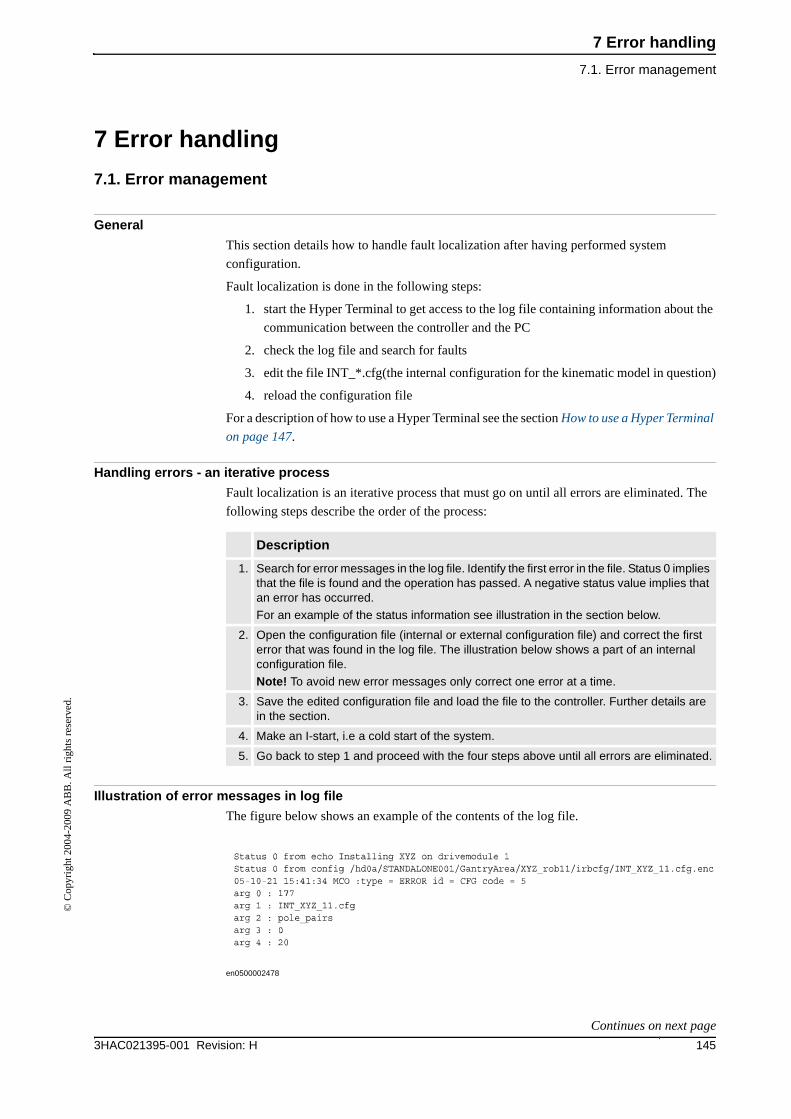
7 Error handling
7.1. Error management
1453HAC021395-001 Revision: H
© C
opyr
ight
200
4-20
09 A
BB
. All
righ
ts r
eser
ved.
7 Error handling
7.1. Error management
General
This section details how to handle fault localization after having performed system
configuration.
Fault localization is done in the following steps:
1. start the Hyper Terminal to get access to the log file containing information about the
communication between the controller and the PC
2. check the log file and search for faults
3. edit the file INT_*.cfg(the internal configuration for the kinematic model in question)
4. reload the configuration file
For a description of how to use a Hyper Terminal see the section How to use a Hyper Terminal
on page 147.
Handling errors - an iterative process
Fault localization is an iterative process that must go on until all errors are eliminated. The
following steps describe the order of the process:
Illustration of error messages in log file
The figure below shows an example of the contents of the log file.
en0500002478
Description
1. Search for error messages in the log file. Identify the first error in the file. Status 0 implies that the file is found and the operation has passed. A negative status value implies that an error has occurred.
For an example of the status information see illustration in the section below.
2. Open the configuration file (internal or external configuration file) and correct the first error that was found in the log file. The illustration below shows a part of an internal configuration file.
Note! To avoid new error messages only correct one error at a time.
3. Save the edited configuration file and load the file to the controller. Further details are in the section.
4. Make an I-start, i.e a cold start of the system.
5. Go back to step 1 and proceed with the four steps above until all errors are eliminated.
Continues on next page
7 Error handling
7.1. Error management
3HAC021395-001 Revision: H146
© C
opyr
ight
200
4-20
09 A
BB
. All
righ
ts r
eser
ved.
Examples of error messages
The table below gives some examples of common error messages that can show up in the log
file after system configuration.
Summary
Error management is necessary to secure that the right configuration file for a certain
kinematic model is used. It is also important to check that parameter settings have been done
with correct/allowed values.
Every time a new system configuration is done or axes are tuned, fault localization and error
correction must also be done to ensure that any remaining errors will be eliminated.
Error message in log fileDescription - cause of failure
How to correct the error
04-01-13 16:33:46 MC0: param.c 1286 cfg_get_named_instance for 'DRIVE_UNIT' ’M2DM1’ failed.
With regard to hardware drive unit position and node position; do not exist for axis rob11_2.
Check the hardware and set the correct node values for the parameter use_drive_unit, in the INT_XYZ_11.cfg file. The parameter is described in the section.
04-01-13 17:43:59 MC0: cfg_file.c 2142
Mandatory attribute 'name' missing in line 180
Status -13 from config compr:/hd0a/STANDALONE001/GantryArea/XYZ_rob11/irbcfg/INT_XYZ_11.cfg.enc
In this case, the sign for the line breaking, "\", is missing on line 179 in the INT_XYZ_11.cfg file.
The error message indicates that the error exists in some of the lines before line 180.
Check the lines for missing or incorrect signs.
04-01-13 17:50:57 MC0: type = ERROR id = SYSTEM code = 136
arg 0: pole_pairs
arg 1: 180
Status -12 from config compr:/hd0a/STANDALONE001/GantryArea/XYZ_rob11/irbcfg/INT_XYZ_11.cfg.enc
The value of pole_pairs (in this case, on line 179) in the INT_XYZ_11.cfg file is not within the permitted limits.
The error message indicates that the error exists in the parameter pole_pairs, in some of the lines before line 180.
Change the value of the parameter pole_pairs in the INT_XYZ_11.cfg file. The parameter and permitted limits are described in the section
Continued
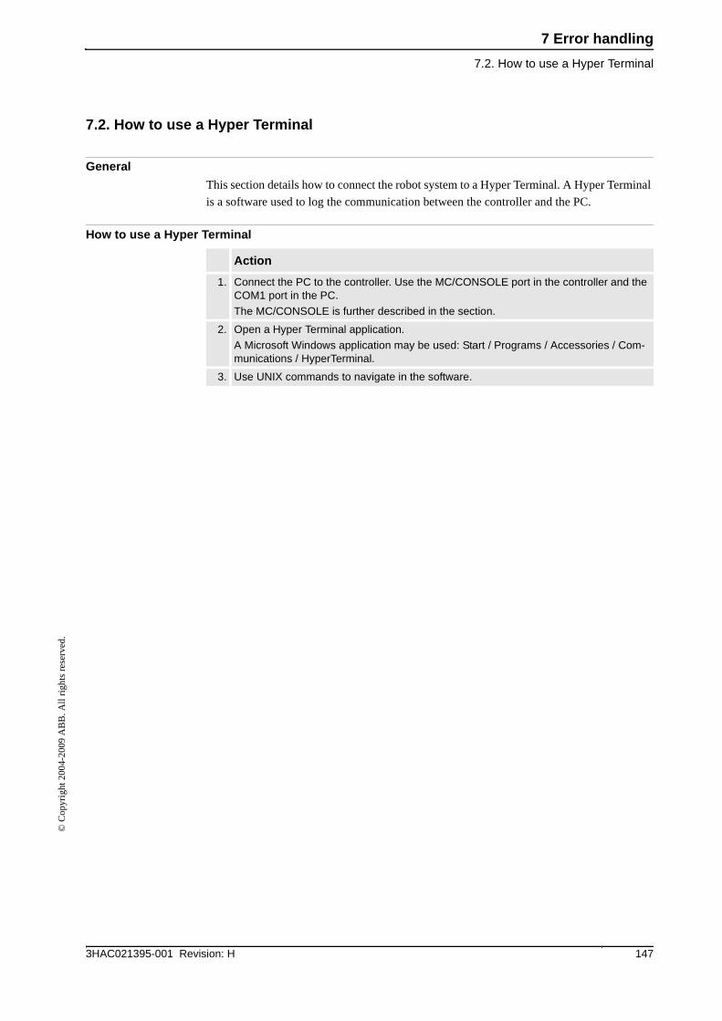
7 Error handling
7.2. How to use a Hyper Terminal
1473HAC021395-001 Revision: H
© C
opyr
ight
200
4-20
09 A
BB
. All
righ
ts r
eser
ved.
7.2. How to use a Hyper Terminal
General
This section details how to connect the robot system to a Hyper Terminal. A Hyper Terminal
is a software used to log the communication between the controller and the PC.
How to use a Hyper Terminal
Action
1. Connect the PC to the controller. Use the MC/CONSOLE port in the controller and the COM1 port in the PC.
The MC/CONSOLE is further described in the section.
2. Open a Hyper Terminal application.
A Microsoft Windows application may be used: Start / Programs / Accessories / Com-munications / HyperTerminal.
3. Use UNIX commands to navigate in the software.

7 Error handling
7.2. How to use a Hyper Terminal
3HAC021395-001 Revision: H148
© C
opyr
ight
200
4-20
09 A
BB
. All
righ
ts r
eser
ved.
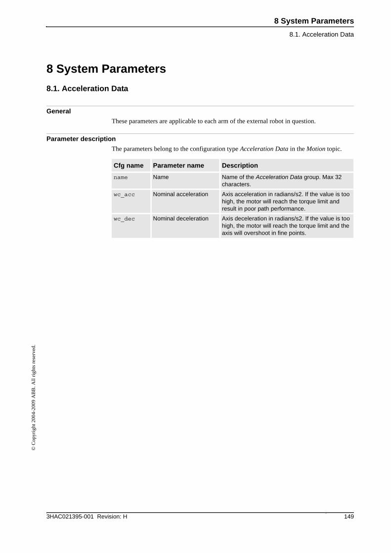
8 System Parameters
8.1. Acceleration Data
1493HAC021395-001 Revision: H
© C
opyr
ight
200
4-20
09 A
BB
. All
righ
ts r
eser
ved.
8 System Parameters
8.1. Acceleration Data
General
These parameters are applicable to each arm of the external robot in question.
Parameter description
The parameters belong to the configuration type Acceleration Data in the Motion topic.
Cfg name Parameter name Description
name Name Name of the Acceleration Data group. Max 32 characters.
wc_acc Nominal acceleration Axis acceleration in radians/s2. If the value is too high, the motor will reach the torque limit and result in poor path performance.
wc_dec Nominal deceleration Axis deceleration in radians/s2. If the value is too high, the motor will reach the torque limit and the axis will overshoot in fine points.
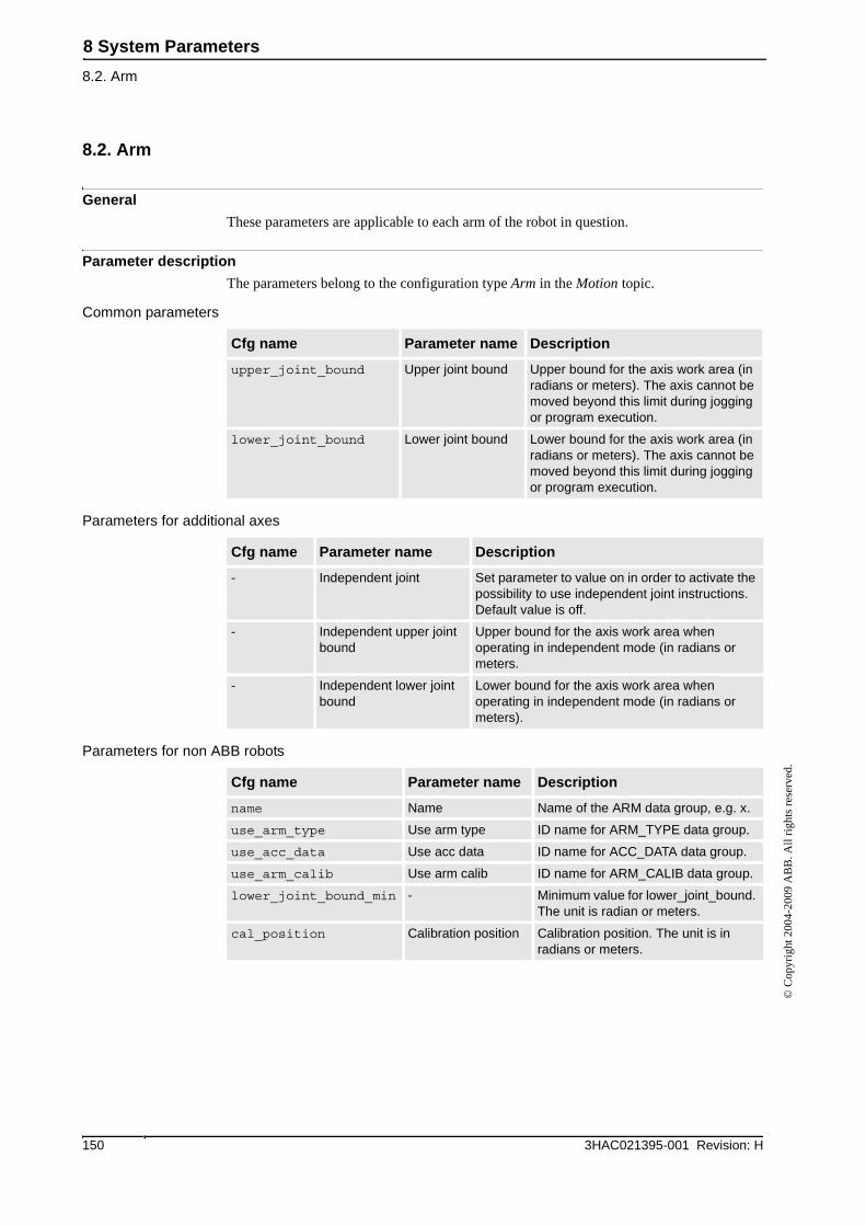
8 System Parameters
8.2. Arm
3HAC021395-001 Revision: H150
© C
opyr
ight
200
4-20
09 A
BB
. All
righ
ts r
eser
ved.
8.2. Arm
General
These parameters are applicable to each arm of the robot in question.
Parameter description
The parameters belong to the configuration type Arm in the Motion topic.
Common parameters
Parameters for additional axes
Parameters for non ABB robots
Cfg name Parameter name Description
upper_joint_bound Upper joint bound Upper bound for the axis work area (in radians or meters). The axis cannot be moved beyond this limit during jogging or program execution.
lower_joint_bound Lower joint bound Lower bound for the axis work area (in radians or meters). The axis cannot be moved beyond this limit during jogging or program execution.
Cfg name Parameter name Description
- Independent joint Set parameter to value on in order to activate the possibility to use independent joint instructions. Default value is off.
- Independent upper joint bound
Upper bound for the axis work area when operating in independent mode (in radians or meters.
- Independent lower joint bound
Lower bound for the axis work area when operating in independent mode (in radians or meters).
Cfg name Parameter name Description
name Name Name of the ARM data group, e.g. x.
use_arm_type Use arm type ID name for ARM_TYPE data group.
use_acc_data Use acc data ID name for ACC_DATA data group.
use_arm_calib Use arm calib ID name for ARM_CALIB data group.
lower_joint_bound_min - Minimum value for lower_joint_bound. The unit is radian or meters.
cal_position Calibration position Calibration position. The unit is in radians or meters.
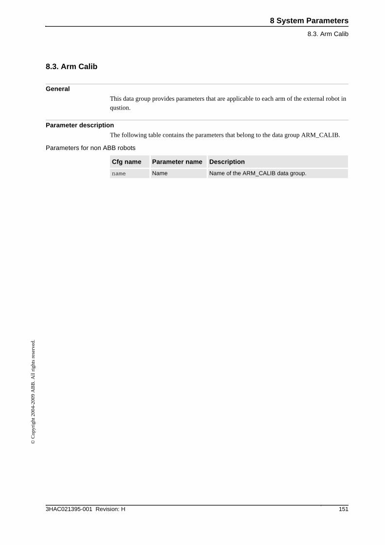
8 System Parameters
8.3. Arm Calib
1513HAC021395-001 Revision: H
© C
opyr
ight
200
4-20
09 A
BB
. All
righ
ts r
eser
ved.
8.3. Arm Calib
General
This data group provides parameters that are applicable to each arm of the external robot in
qustion.
Parameter description
The following table contains the parameters that belong to the data group ARM_CALIB.
Parameters for non ABB robots
Cfg name Parameter name Description
name Name Name of the ARM_CALIB data group.
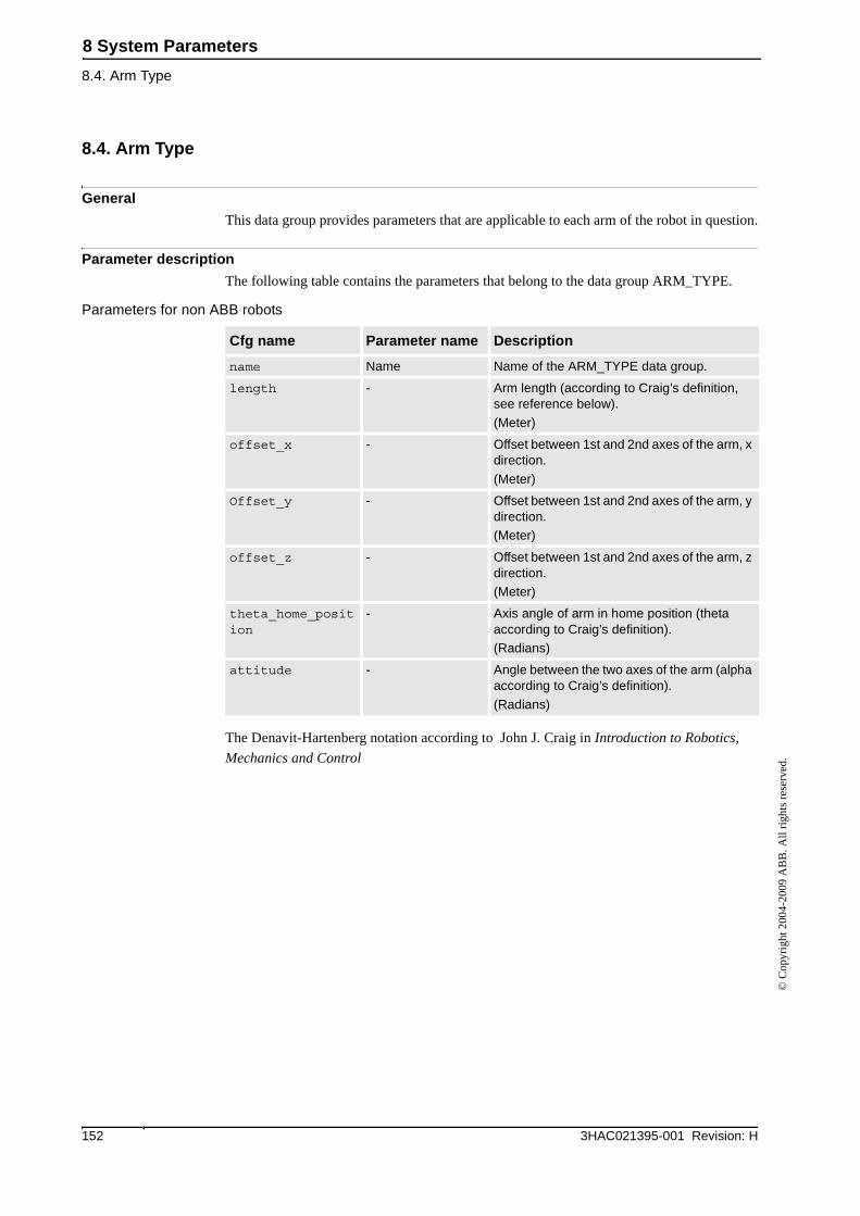
8 System Parameters
8.4. Arm Type
3HAC021395-001 Revision: H152
© C
opyr
ight
200
4-20
09 A
BB
. All
righ
ts r
eser
ved.
8.4. Arm Type
General
This data group provides parameters that are applicable to each arm of the robot in question.
Parameter description
The following table contains the parameters that belong to the data group ARM_TYPE.
Parameters for non ABB robots
The Denavit-Hartenberg notation according to John J. Craig in Introduction to Robotics,
Mechanics and Control
Cfg name Parameter name Description
name Name Name of the ARM_TYPE data group.
length - Arm length (according to Craig’s definition, see reference below).
(Meter)
offset_x - Offset between 1st and 2nd axes of the arm, x direction.
(Meter)
Offset_y - Offset between 1st and 2nd axes of the arm, y direction.
(Meter)
offset_z - Offset between 1st and 2nd axes of the arm, z direction.
(Meter)
theta_home_position
- Axis angle of arm in home position (theta according to Craig’s definition).
(Radians)
attitude - Angle between the two axes of the arm (alpha according to Craig’s definition).
(Radians)
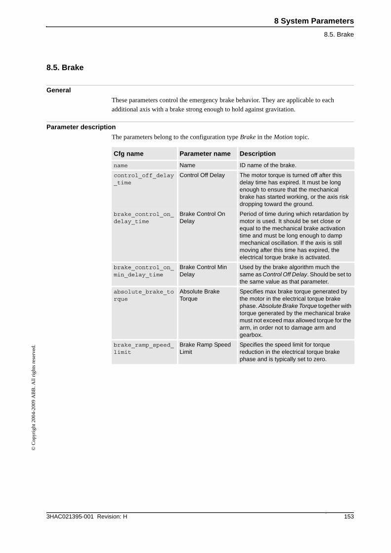
8 System Parameters
8.5. Brake
1533HAC021395-001 Revision: H
© C
opyr
ight
200
4-20
09 A
BB
. All
righ
ts r
eser
ved.
8.5. Brake
General
These parameters control the emergency brake behavior. They are applicable to each
additional axis with a brake strong enough to hold against gravitation.
Parameter description
The parameters belong to the configuration type Brake in the Motion topic.
Cfg name Parameter name Description
name Name ID name of the brake.
control_off_delay_time
Control Off Delay The motor torque is turned off after this delay time has expired. It must be long enough to ensure that the mechanical brake has started working, or the axis risk dropping toward the ground.
brake_control_on_delay_time
Brake Control On Delay
Period of time during which retardation by motor is used. It should be set close or equal to the mechanical brake activation time and must be long enough to damp mechanical oscillation. If the axis is still moving after this time has expired, the electrical torque brake is activated.
brake_control_on_min_delay_time
Brake Control Min Delay
Used by the brake algorithm much the same as Control Off Delay. Should be set to the same value as that parameter.
absolute_brake_torque
Absolute Brake Torque
Specifies max brake torque generated by the motor in the electrical torque brake phase. Absolute Brake Torque together with torque generated by the mechanical brake must not exceed max allowed torque for the arm, in order not to damage arm and gearbox.
brake_ramp_speed_limit
Brake Ramp Speed Limit
Specifies the speed limit for torque reduction in the electrical torque brake phase and is typically set to zero.
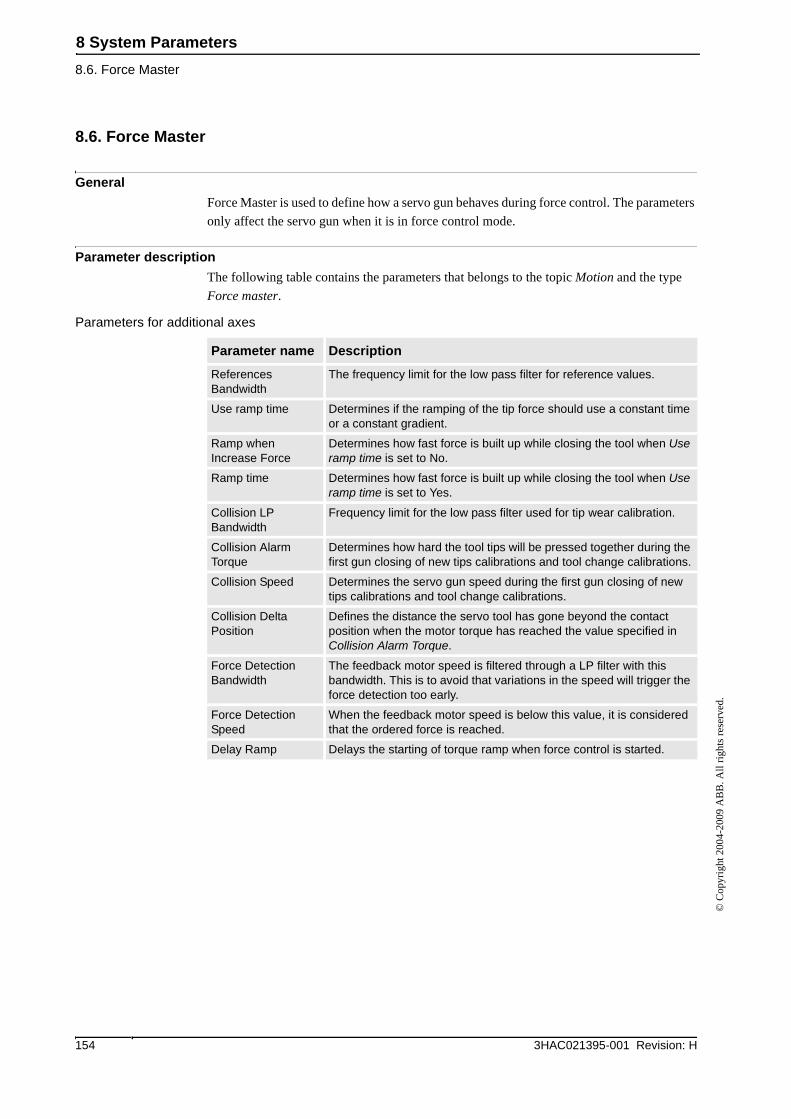
8 System Parameters
8.6. Force Master
3HAC021395-001 Revision: H154
© C
opyr
ight
200
4-20
09 A
BB
. All
righ
ts r
eser
ved.
8.6. Force Master
General
Force Master is used to define how a servo gun behaves during force control. The parameters
only affect the servo gun when it is in force control mode.
Parameter description
The following table contains the parameters that belongs to the topic Motion and the type
Force master.
Parameters for additional axes
Parameter name Description
References Bandwidth
The frequency limit for the low pass filter for reference values.
Use ramp time Determines if the ramping of the tip force should use a constant time or a constant gradient.
Ramp when Increase Force
Determines how fast force is built up while closing the tool when Use ramp time is set to No.
Ramp time Determines how fast force is built up while closing the tool when Use ramp time is set to Yes.
Collision LP Bandwidth
Frequency limit for the low pass filter used for tip wear calibration.
Collision Alarm Torque
Determines how hard the tool tips will be pressed together during the first gun closing of new tips calibrations and tool change calibrations.
Collision Speed Determines the servo gun speed during the first gun closing of new tips calibrations and tool change calibrations.
Collision Delta Position
Defines the distance the servo tool has gone beyond the contact position when the motor torque has reached the value specified in Collision Alarm Torque.
Force Detection Bandwidth
The feedback motor speed is filtered through a LP filter with this bandwidth. This is to avoid that variations in the speed will trigger the force detection too early.
Force Detection Speed
When the feedback motor speed is below this value, it is considered that the ordered force is reached.
Delay Ramp Delays the starting of torque ramp when force control is started.
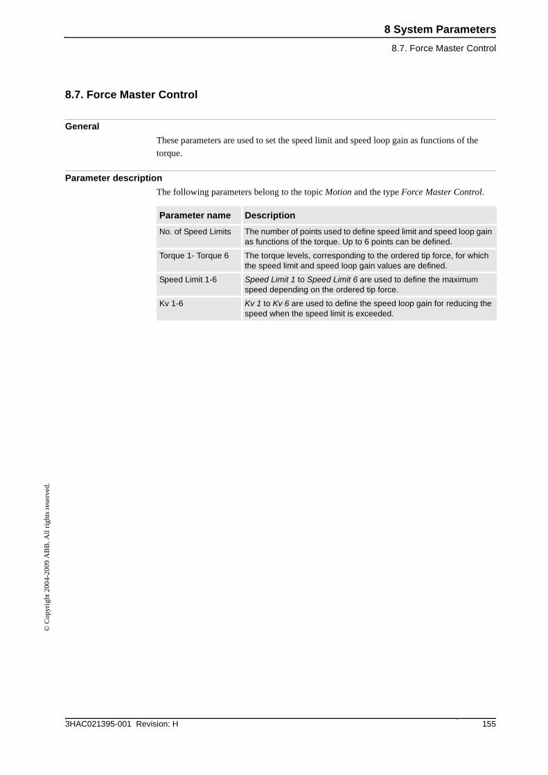
8 System Parameters
8.7. Force Master Control
1553HAC021395-001 Revision: H
© C
opyr
ight
200
4-20
09 A
BB
. All
righ
ts r
eser
ved.
8.7. Force Master Control
General
These parameters are used to set the speed limit and speed loop gain as functions of the
torque.
Parameter description
The following parameters belong to the topic Motion and the type Force Master Control.
Parameter name Description
No. of Speed Limits The number of points used to define speed limit and speed loop gain as functions of the torque. Up to 6 points can be defined.
Torque 1- Torque 6 The torque levels, corresponding to the ordered tip force, for which the speed limit and speed loop gain values are defined.
Speed Limit 1-6 Speed Limit 1 to Speed Limit 6 are used to define the maximum speed depending on the ordered tip force.
Kv 1-6 Kv 1 to Kv 6 are used to define the speed loop gain for reducing the speed when the speed limit is exceeded.
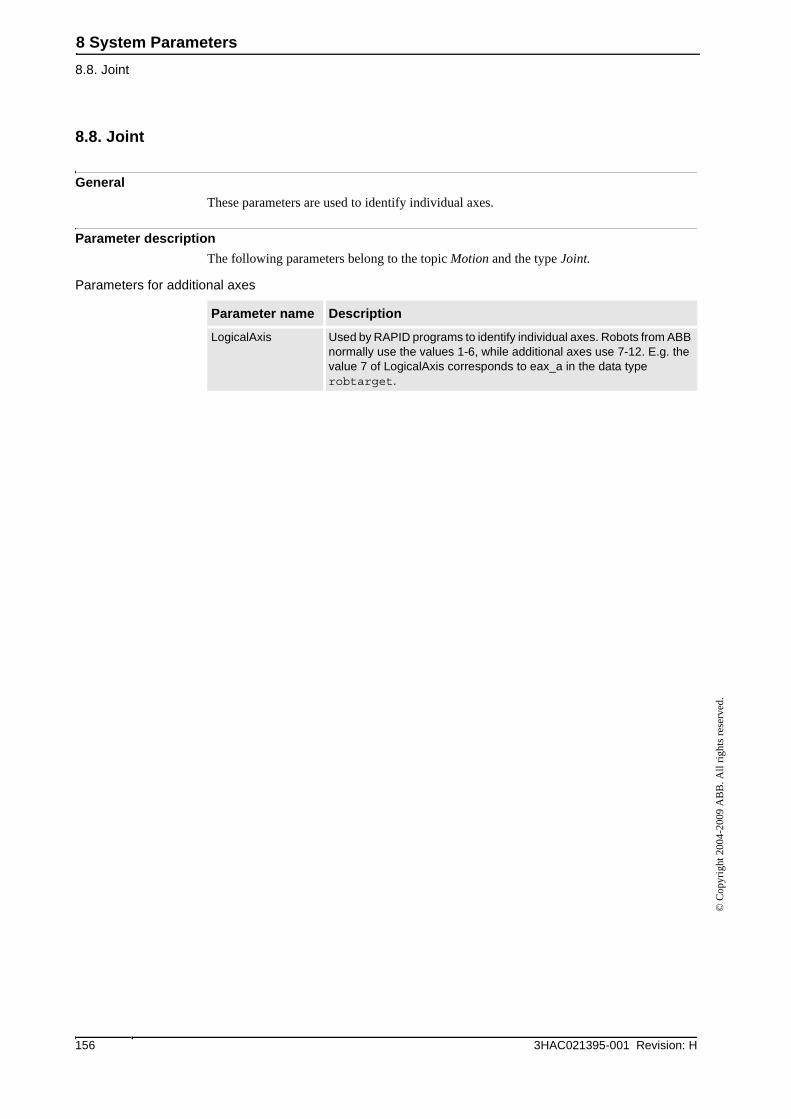
8 System Parameters
8.8. Joint
3HAC021395-001 Revision: H156
© C
opyr
ight
200
4-20
09 A
BB
. All
righ
ts r
eser
ved.
8.8. Joint
General
These parameters are used to identify individual axes.
Parameter description
The following parameters belong to the topic Motion and the type Joint.
Parameters for additional axes
Parameter name Description
LogicalAxis Used by RAPID programs to identify individual axes. Robots from ABB normally use the values 1-6, while additional axes use 7-12. E.g. the value 7 of LogicalAxis corresponds to eax_a in the data type robtarget.
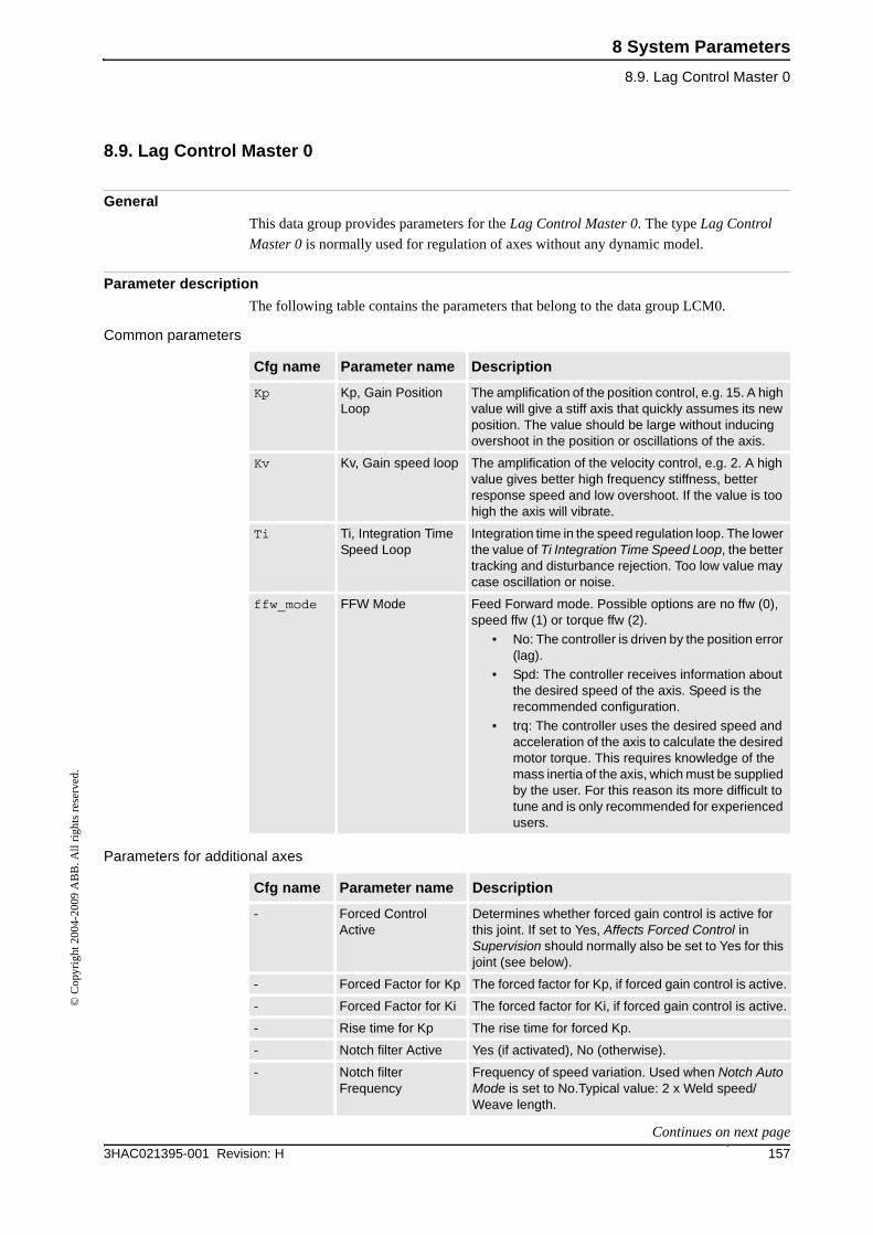
8 System Parameters
8.9. Lag Control Master 0
1573HAC021395-001 Revision: H
© C
opyr
ight
200
4-20
09 A
BB
. All
righ
ts r
eser
ved.
8.9. Lag Control Master 0
General
This data group provides parameters for the Lag Control Master 0. The type Lag Control
Master 0 is normally used for regulation of axes without any dynamic model.
Parameter description
The following table contains the parameters that belong to the data group LCM0.
Common parameters
Parameters for additional axes
Cfg name Parameter name Description
Kp Kp, Gain Position Loop
The amplification of the position control, e.g. 15. A high value will give a stiff axis that quickly assumes its new position. The value should be large without inducing overshoot in the position or oscillations of the axis.
Kv Kv, Gain speed loop The amplification of the velocity control, e.g. 2. A high value gives better high frequency stiffness, better response speed and low overshoot. If the value is too high the axis will vibrate.
Ti Ti, Integration Time Speed Loop
Integration time in the speed regulation loop. The lower the value of Ti Integration Time Speed Loop, the better tracking and disturbance rejection. Too low value may case oscillation or noise.
ffw_mode FFW Mode Feed Forward mode. Possible options are no ffw (0), speed ffw (1) or torque ffw (2).
• No: The controller is driven by the position error (lag).
• Spd: The controller receives information about the desired speed of the axis. Speed is the recommended configuration.
• trq: The controller uses the desired speed and acceleration of the axis to calculate the desired motor torque. This requires knowledge of the mass inertia of the axis, which must be supplied by the user. For this reason its more difficult to tune and is only recommended for experienced users.
Cfg name Parameter name Description
- Forced Control Active
Determines whether forced gain control is active for this joint. If set to Yes, Affects Forced Control in Supervision should normally also be set to Yes for this joint (see below).
- Forced Factor for Kp The forced factor for Kp, if forced gain control is active.
- Forced Factor for Ki The forced factor for Ki, if forced gain control is active.
- Rise time for Kp The rise time for forced Kp.
- Notch filter Active Yes (if activated), No (otherwise).
- Notch filter Frequency
Frequency of speed variation. Used when Notch Auto Mode is set to No.Typical value: 2 x Weld speed/Weave length.
Continues on next page
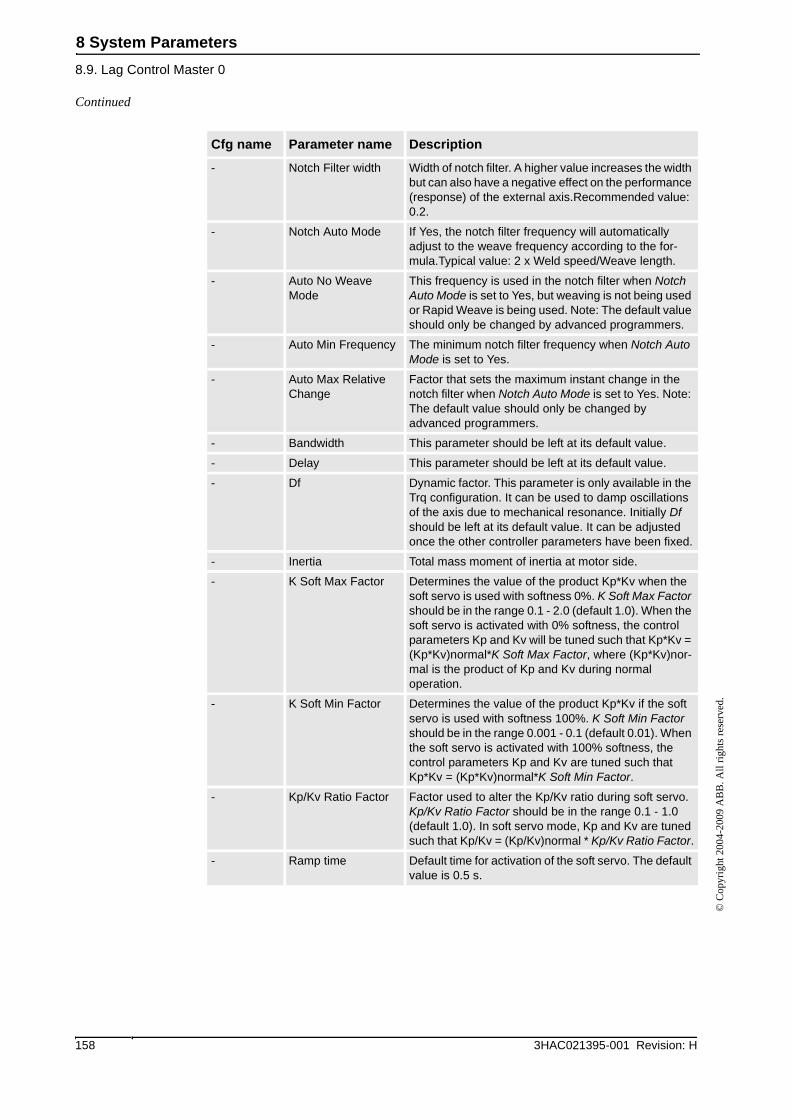
8 System Parameters
8.9. Lag Control Master 0
3HAC021395-001 Revision: H158
© C
opyr
ight
200
4-20
09 A
BB
. All
righ
ts r
eser
ved.
- Notch Filter width Width of notch filter. A higher value increases the width but can also have a negative effect on the performance (response) of the external axis.Recommended value: 0.2.
- Notch Auto Mode If Yes, the notch filter frequency will automatically adjust to the weave frequency according to the for-mula.Typical value: 2 x Weld speed/Weave length.
- Auto No Weave Mode
This frequency is used in the notch filter when Notch Auto Mode is set to Yes, but weaving is not being used or Rapid Weave is being used. Note: The default value should only be changed by advanced programmers.
- Auto Min Frequency The minimum notch filter frequency when Notch Auto Mode is set to Yes.
- Auto Max Relative Change
Factor that sets the maximum instant change in the notch filter when Notch Auto Mode is set to Yes. Note: The default value should only be changed by advanced programmers.
- Bandwidth This parameter should be left at its default value.
- Delay This parameter should be left at its default value.
- Df Dynamic factor. This parameter is only available in the Trq configuration. It can be used to damp oscillations of the axis due to mechanical resonance. Initially Df should be left at its default value. It can be adjusted once the other controller parameters have been fixed.
- Inertia Total mass moment of inertia at motor side.
- K Soft Max Factor Determines the value of the product Kp*Kv when the soft servo is used with softness 0%. K Soft Max Factor should be in the range 0.1 - 2.0 (default 1.0). When the soft servo is activated with 0% softness, the control parameters Kp and Kv will be tuned such that Kp*Kv = (Kp*Kv)normal*K Soft Max Factor, where (Kp*Kv)nor-mal is the product of Kp and Kv during normal operation.
- K Soft Min Factor Determines the value of the product Kp*Kv if the soft servo is used with softness 100%. K Soft Min Factor should be in the range 0.001 - 0.1 (default 0.01). When the soft servo is activated with 100% softness, the control parameters Kp and Kv are tuned such that Kp*Kv = (Kp*Kv)normal*K Soft Min Factor.
- Kp/Kv Ratio Factor Factor used to alter the Kp/Kv ratio during soft servo. Kp/Kv Ratio Factor should be in the range 0.1 - 1.0 (default 1.0). In soft servo mode, Kp and Kv are tuned such that Kp/Kv = (Kp/Kv)normal * Kp/Kv Ratio Factor.
- Ramp time Default time for activation of the soft servo. The default value is 0.5 s.
Cfg name Parameter name Description
Continued
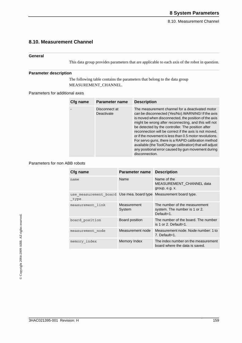
8 System Parameters
8.10. Measurement Channel
1593HAC021395-001 Revision: H
© C
opyr
ight
200
4-20
09 A
BB
. All
righ
ts r
eser
ved.
8.10. Measurement Channel
General
This data group provides parameters that are applicable to each axis of the robot in question.
Parameter description
The following table contains the parameters that belong to the data group
MEASUREMENT_CHANNEL.
Parameters for additional axes
Parameters for non ABB robots
Cfg name Parameter name Description
- Disconnect at Deactivate
The measurement channel for a deactivated motor can be disconnected (Yes/No).WARNING! If the axis is moved when disconnected, the position of the axis might be wrong after reconnecting, and this will not be detected by the controller. The position after reconnection will be correct if the axis is not moved, or if the movement is less than 0.5 motor revolutions. For servo guns, there is a RAPID calibration method available (the ToolChange calibration) that will adjust any positional error caused by gun movement during disconnection.
Cfg name Parameter name Description
name Name Name of the MEASUREMENT_CHANNEL data group, e.g. x.
use_measurement_board_type
Use mea. board type Measurement board type.
measurement_link Measurement System
The number of the measurement system. The number is 1 or 2. Default=1.
board_position Board position The number of the board. The number is 1 or 2. Default=1.
measurement_node Measurement node Measurement node. Node number: 1 to 7. Default=1.
memory_index Memory Index The index number on the measurement board where the data is saved.
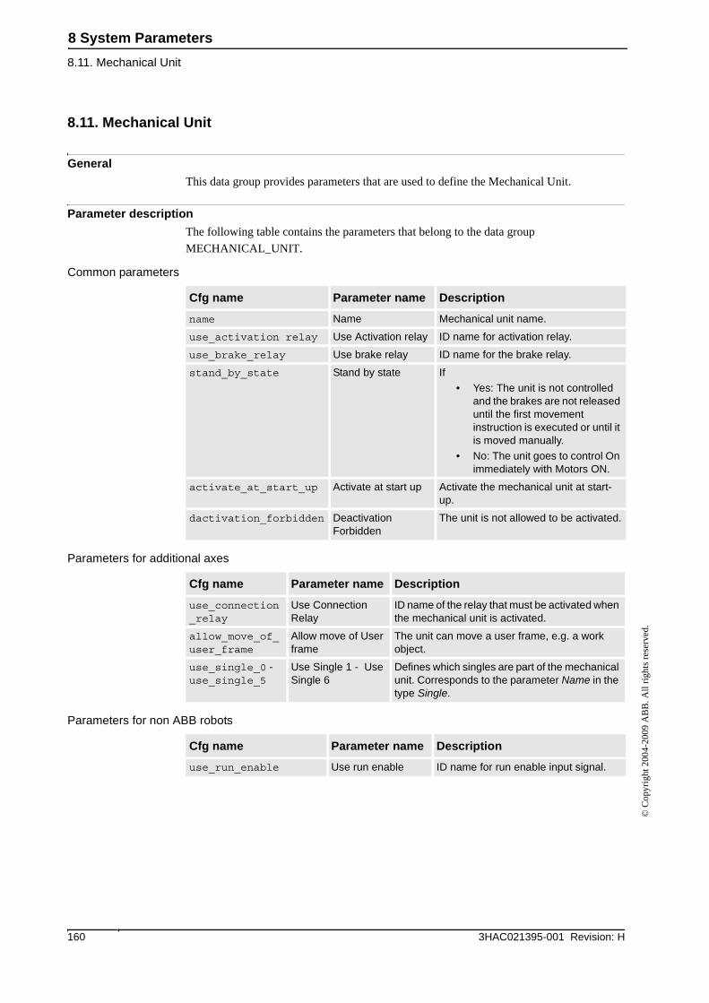
8 System Parameters
8.11. Mechanical Unit
3HAC021395-001 Revision: H160
© C
opyr
ight
200
4-20
09 A
BB
. All
righ
ts r
eser
ved.
8.11. Mechanical Unit
General
This data group provides parameters that are used to define the Mechanical Unit.
Parameter description
The following table contains the parameters that belong to the data group
MECHANICAL_UNIT.
Common parameters
Parameters for additional axes
Parameters for non ABB robots
Cfg name Parameter name Description
name Name Mechanical unit name.
use_activation relay Use Activation relay ID name for activation relay.
use_brake_relay Use brake relay ID name for the brake relay.
stand_by_state Stand by state If
• Yes: The unit is not controlled and the brakes are not released until the first movement instruction is executed or until it is moved manually.
• No: The unit goes to control On immediately with Motors ON.
activate_at_start_up Activate at start up Activate the mechanical unit at start-up.
dactivation_forbidden Deactivation Forbidden
The unit is not allowed to be activated.
Cfg name Parameter name Description
use_connection_relay
Use Connection Relay
ID name of the relay that must be activated when the mechanical unit is activated.
allow_move_of_user_frame
Allow move of User frame
The unit can move a user frame, e.g. a work object.
use_single_0 - use_single_5
Use Single 1 - Use Single 6
Defines which singles are part of the mechanical unit. Corresponds to the parameter Name in the type Single.
Cfg name Parameter name Description
use_run_enable Use run enable ID name for run enable input signal.
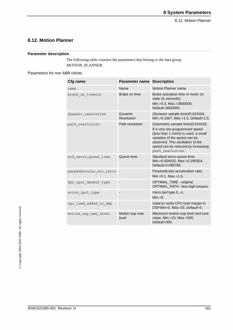
8 System Parameters
8.12. Motion Planner
1613HAC021395-001 Revision: H
© C
opyr
ight
200
4-20
09 A
BB
. All
righ
ts r
eser
ved.
8.12. Motion Planner
Parameter description
The following table contains the parameters that belong to the data group
MOTION_PLANNER.
Parameters for non ABB robots
Cfg name Parameter name Description
name Name Motion Planner name.
brake_on_timeout Brake on time Brake activation time in motor on state (in seconds).
Min.=0.3, Max.=3600000, Default=3600000.
dynamic_resolution Dynamic Resolution
(Dynamic sample time)/0.024192. Min.=0.1667, Max.=1.0, Default=1.0.
path_resolution Path resolution (Geometric sample time)/0.024192.
If a very low programmed speed (less than 1 mm/s) is used, a small variation of the speed can be observed. This oscillation of the speed can be reduced by increasing path_resolution.
std_servo_queue_time Queue time Standard servo queue time. Min.=0.004032, Max.=0.290304, Default=0.096768.
perpendicular_acc_ratio - Perpendicular acceleration ratio.
Min.=0.1, Max.=1.5.
dyn_ipol_decbuf_type - OPTIMAL_TIME - original, OPTIMAL_PATH - less high torques.
micro_ipol_type - micro ipol type 0,.,n.
Min.=0.
cpu_load_added_to_dsp - Used to verify CPU load margin in DSP.Min=0, Max=25, Default=0.
motion_sup_max_level Motion sup max level
Maximum motion sup level and tune value. Min.=10, Max.=500, Default=300.
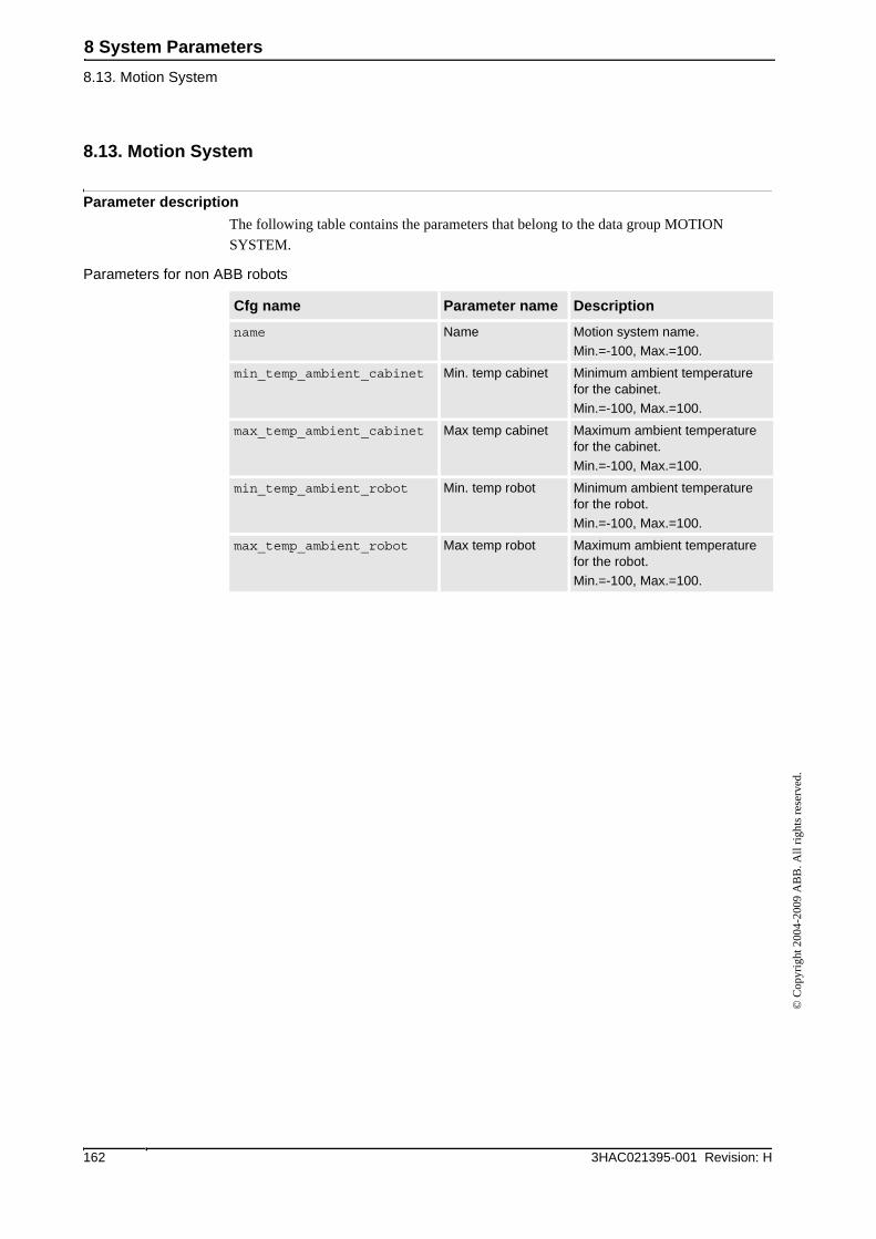
8 System Parameters
8.13. Motion System
3HAC021395-001 Revision: H162
© C
opyr
ight
200
4-20
09 A
BB
. All
righ
ts r
eser
ved.
8.13. Motion System
Parameter description
The following table contains the parameters that belong to the data group MOTION
SYSTEM.
Parameters for non ABB robots
Cfg name Parameter name Description
name Name Motion system name.
Min.=-100, Max.=100.
min_temp_ambient_cabinet Min. temp cabinet Minimum ambient temperature for the cabinet.
Min.=-100, Max.=100.
max_temp_ambient_cabinet Max temp cabinet Maximum ambient temperature for the cabinet.
Min.=-100, Max.=100.
min_temp_ambient_robot Min. temp robot Minimum ambient temperature for the robot.
Min.=-100, Max.=100.
max_temp_ambient_robot Max temp robot Maximum ambient temperature for the robot.
Min.=-100, Max.=100.
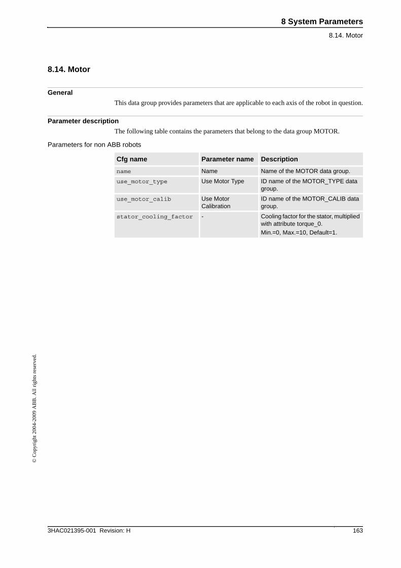
8 System Parameters
8.14. Motor
1633HAC021395-001 Revision: H
© C
opyr
ight
200
4-20
09 A
BB
. All
righ
ts r
eser
ved.
8.14. Motor
General
This data group provides parameters that are applicable to each axis of the robot in question.
Parameter description
The following table contains the parameters that belong to the data group MOTOR.
Parameters for non ABB robots
Cfg name Parameter name Description
name Name Name of the MOTOR data group.
use_motor_type Use Motor Type ID name of the MOTOR_TYPE data group.
use_motor_calib Use Motor Calibration
ID name of the MOTOR_CALIB data group.
stator_cooling_factor - Cooling factor for the stator, multiplied with attribute torque_0.
Min.=0, Max.=10, Default=1.
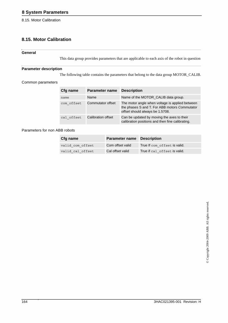
8 System Parameters
8.15. Motor Calibration
3HAC021395-001 Revision: H164
© C
opyr
ight
200
4-20
09 A
BB
. All
righ
ts r
eser
ved.
8.15. Motor Calibration
General
This data group provides parameters that are applicable to each axis of the robot in question
Parameter description
The following table contains the parameters that belong to the data group MOTOR_CALIB.
Common parameters
Parameters for non ABB robots
Cfg name Parameter name Description
name Name Name of the MOTOR_CALIB data group.
com_offset Commutator offset The motor angle when voltage is applied between the phases S and T. For ABB motors Commutator offset should always be 1.5708.
cal_offset Calibration offset Can be updated by moving the axes to their calibration positions and then fine calibrating.
Cfg name Parameter name Description
valid_com_offset Com offset valid True If com_offset is valid.
valid_cal_offset Cal offset valid True if cal_offset is valid.
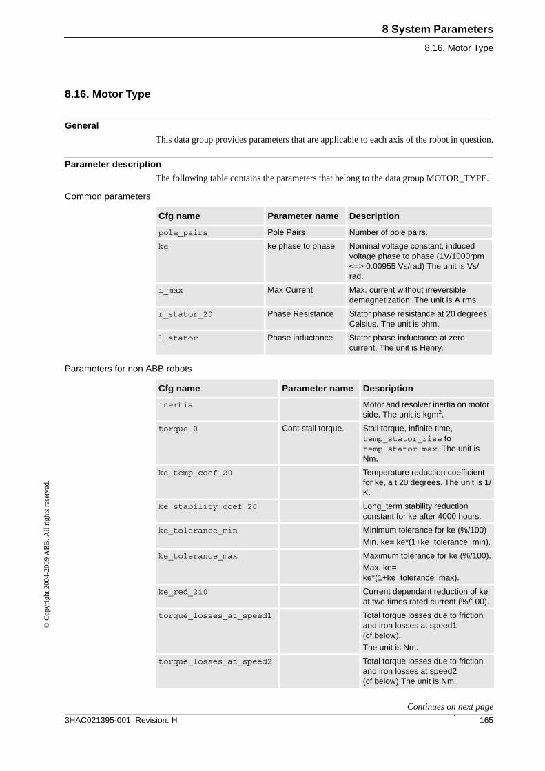
8 System Parameters
8.16. Motor Type
1653HAC021395-001 Revision: H
© C
opyr
ight
200
4-20
09 A
BB
. All
righ
ts r
eser
ved.
8.16. Motor Type
General
This data group provides parameters that are applicable to each axis of the robot in question.
Parameter description
The following table contains the parameters that belong to the data group MOTOR_TYPE.
Common parameters
Parameters for non ABB robots
Cfg name Parameter name Description
pole_pairs Pole Pairs Number of pole pairs.
ke ke phase to phase Nominal voltage constant, induced voltage phase to phase (1V/1000rpm <=> 0.00955 Vs/rad) The unit is Vs/rad.
i_max Max Current Max. current without irreversible demagnetization. The unit is A rms.
r_stator_20 Phase Resistance Stator phase resistance at 20 degrees Celsius. The unit is ohm.
l_stator Phase inductance Stator phase inductance at zero current. The unit is Henry.
Cfg name Parameter name Description
inertia Motor and resolver inertia on motor side. The unit is kgm2.
torque_0 Cont stall torque. Stall torque, infinite time, temp_stator_rise to temp_stator_max. The unit is Nm.
ke_temp_coef_20 Temperature reduction coefficient for ke, a t 20 degrees. The unit is 1/K.
ke_stability_coef_20 Long_term stability reduction constant for ke after 4000 hours.
ke_tolerance_min Minimum tolerance for ke (%/100)
Min. ke= ke*(1+ke_tolerance_min).
ke_tolerance_max Maximum tolerance for ke (%/100).
Max. ke= ke*(1+ke_tolerance_max).
ke_red_2i0 Current dependant reduction of ke at two times rated current (%/100).
torque_losses_at_speed1 Total torque losses due to friction and iron losses at speed1 (cf.below).
The unit is Nm.
torque_losses_at_speed2 Total torque losses due to friction and iron losses at speed2 (cf.below).The unit is Nm.
Continues on next page
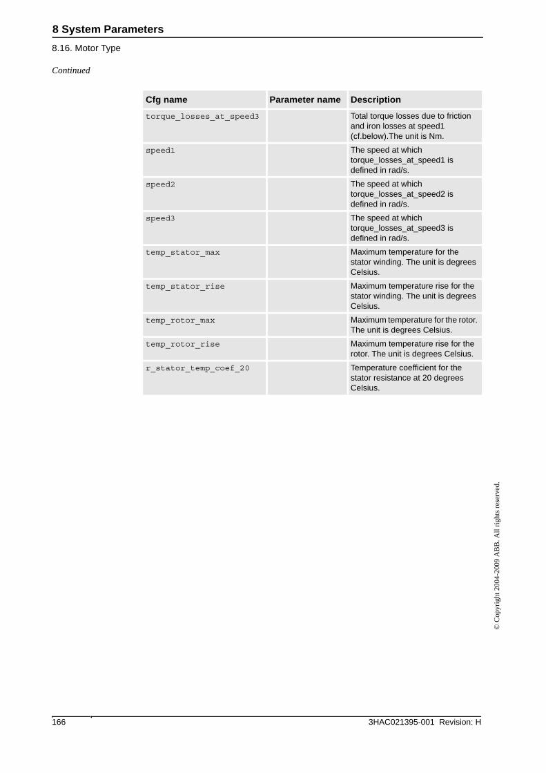
8 System Parameters
8.16. Motor Type
3HAC021395-001 Revision: H166
© C
opyr
ight
200
4-20
09 A
BB
. All
righ
ts r
eser
ved.
torque_losses_at_speed3 Total torque losses due to friction and iron losses at speed1 (cf.below).The unit is Nm.
speed1 The speed at which torque_losses_at_speed1 is defined in rad/s.
speed2 The speed at which torque_losses_at_speed2 is defined in rad/s.
speed3 The speed at which torque_losses_at_speed3 is defined in rad/s.
temp_stator_max Maximum temperature for the stator winding. The unit is degrees Celsius.
temp_stator_rise Maximum temperature rise for the stator winding. The unit is degrees Celsius.
temp_rotor_max Maximum temperature for the rotor. The unit is degrees Celsius.
temp_rotor_rise Maximum temperature rise for the rotor. The unit is degrees Celsius.
r_stator_temp_coef_20 Temperature coefficient for the stator resistance at 20 degrees Celsius.
Cfg name Parameter name Description
Continued
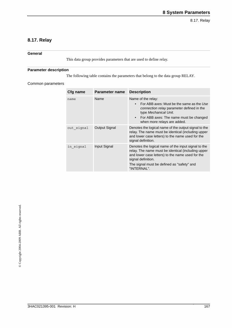
8 System Parameters
8.17. Relay
1673HAC021395-001 Revision: H
© C
opyr
ight
200
4-20
09 A
BB
. All
righ
ts r
eser
ved.
8.17. Relay
General
This data group provides parameters that are used to define relay.
Parameter description
The following table contains the parameters that belong to the data group RELAY.
Common parameters
Cfg name Parameter name Description
name Name Name of the relay:
• For ABB axes: Must be the same as the Use connection relay parameter defined in the type Mechanical Unit.
• For ABB axes: The name must be changed when more relays are added.
out_signal Output Signal Denotes the logical name of the output signal to the relay. The name must be identical (including upper and lower case letters) to the name used for the signal definition.
in_signal Input Signal Denotes the logical name of the input signal to the relay. The name must be identical (including upper and lower case letters) to the name used for the signal definition.
The signal must be defined as "safety" and "INTERNAL".
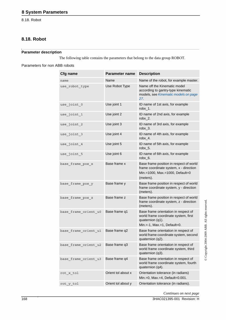
8 System Parameters
8.18. Robot
3HAC021395-001 Revision: H168
© C
opyr
ight
200
4-20
09 A
BB
. All
righ
ts r
eser
ved.
8.18. Robot
Parameter description
The following table contains the parameters that belong to the data group ROBOT.
Parameters for non ABB robots
Cfg name Parameter name Description
name Name Name of the robot, for example master.
use_robot_type Use Robot Type Name off the Kinematic model according to gantry-type kinematic models, see Kinematic models on page 27.
use_joint_0 Use joint 1 ID name of 1st axis, for example robx_1.
use_joint_1 Use joint 2 ID name of 2nd axis, for example robx_2.
use_joint_2 Use joint 3 ID name of 3rd axis, for example robx_3.
use_joint_3 Use joint 4 ID name of 4th axis, for example robx_4.
use_joint_4 Use joint 5 ID name of 5th axis, for example robx_5.
use_joint_5 Use joint 6 ID name of 6th axis, for example robx_6.
base_frame_pos_x Base frame x Base frame position in respect of world frame coordinate system, x - direction
Min.=1000, Max.=1000, Default=0
(meters).
base_frame_pos_y Base frame y Base frame position in respect of world frame coordinate system, y - direction (meters).
base_frame_pos_z Base frame z Base frame position in respect of world frame coordinate system, z - direction (meters).
base_frame_orient_u0 Base frame q1 Base frame orientation in respect of world frame coordinate system, first quaternion (q1).
Min.=-1, Max.=1, Default=0.
base_frame_orient_u1 Base frame q2 Base frame orientation in respect of world frame coordinate system, second quaternion (q2).
base_frame_orient_u2 Base frame q3 Base frame orientation in respect of world frame coordinate system, third quaternion (q3).
base_frame_orient_u3 Base frame q4 Base frame orientation in respect of world frame coordinate system, fourth quaternion (q4).
rot_x_tol Orient tol about x Orientation tolerance (in radians)
Min.=0, Max.=4, Default=0.001.
rot_y_tol Orient tol about y Orientation tolerance (in radians).
Continues on next page
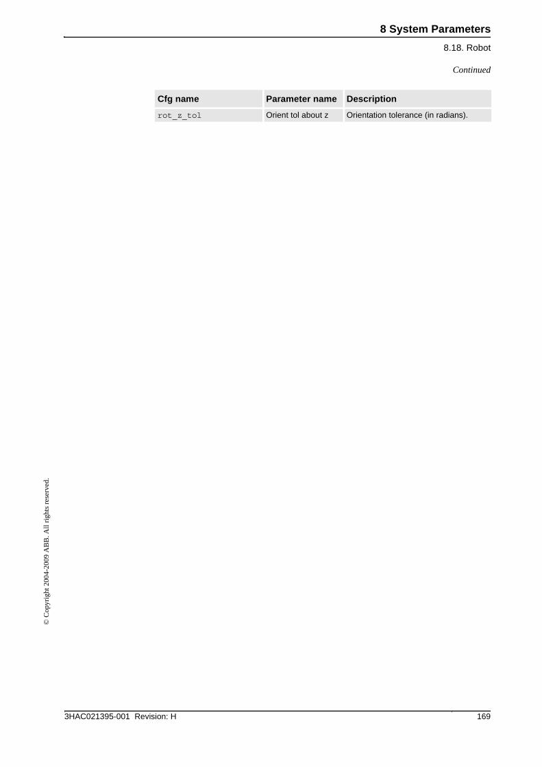
8 System Parameters
8.18. Robot
1693HAC021395-001 Revision: H
© C
opyr
ight
200
4-20
09 A
BB
. All
righ
ts r
eser
ved.
rot_z_tol Orient tol about z Orientation tolerance (in radians).
Cfg name Parameter name Description
Continued
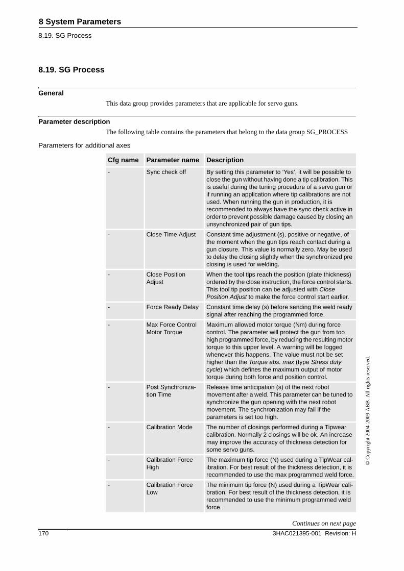
8 System Parameters
8.19. SG Process
3HAC021395-001 Revision: H170
© C
opyr
ight
200
4-20
09 A
BB
. All
righ
ts r
eser
ved.
8.19. SG Process
General
This data group provides parameters that are applicable for servo guns.
Parameter description
The following table contains the parameters that belong to the data group SG_PROCESS
Parameters for additional axes
Cfg name Parameter name Description
- Sync check off By setting this parameter to ‘Yes’, it will be possible to close the gun without having done a tip calibration. This is useful during the tuning procedure of a servo gun or if running an application where tip calibrations are not used. When running the gun in production, it is recommended to always have the sync check active in order to prevent possible damage caused by closing an unsynchronized pair of gun tips.
- Close Time Adjust Constant time adjustment (s), positive or negative, of the moment when the gun tips reach contact during a gun closure. This value is normally zero. May be used to delay the closing slightly when the synchronized pre closing is used for welding.
- Close Position Adjust
When the tool tips reach the position (plate thickness) ordered by the close instruction, the force control starts. This tool tip position can be adjusted with Close Position Adjust to make the force control start earlier.
- Force Ready Delay Constant time delay (s) before sending the weld ready signal after reaching the programmed force.
- Max Force Control Motor Torque
Maximum allowed motor torque (Nm) during force control. The parameter will protect the gun from too high programmed force, by reducing the resulting motor torque to this upper level. A warning will be logged whenever this happens. The value must not be set higher than the Torque abs. max (type Stress duty cycle) which defines the maximum output of motor torque during both force and position control.
- Post Synchroniza-tion Time
Release time anticipation (s) of the next robot movement after a weld. This parameter can be tuned to synchronize the gun opening with the next robot movement. The synchronization may fail if the parameters is set too high.
- Calibration Mode The number of closings performed during a Tipwear calibration. Normally 2 closings will be ok. An increase may improve the accuracy of thickness detection for some servo guns.
- Calibration Force High
The maximum tip force (N) used during a TipWear cal-ibration. For best result of the thickness detection, it is recommended to use the max programmed weld force.
- Calibration Force Low
The minimum tip force (N) used during a TipWear cali-bration. For best result of the thickness detection, it is recommended to use the minimum programmed weld force.
Continues on next page
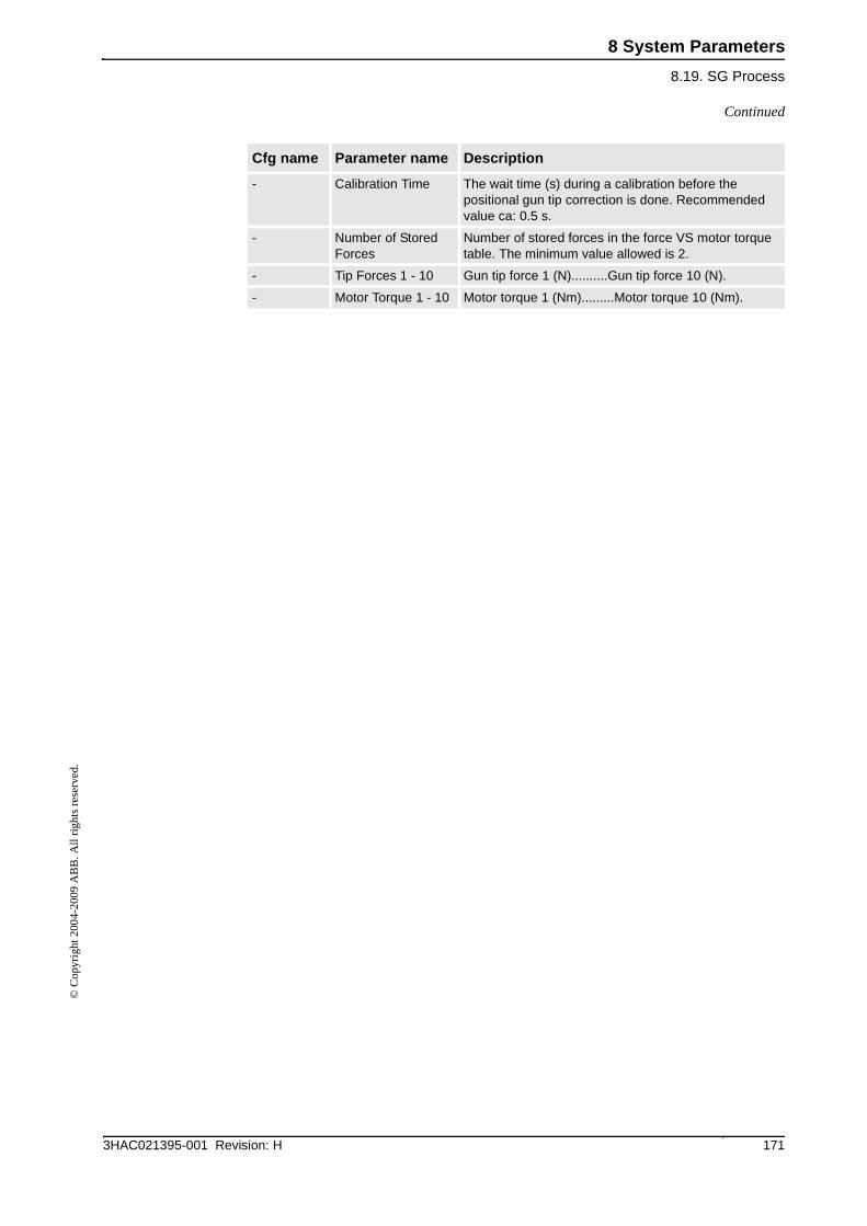
8 System Parameters
8.19. SG Process
1713HAC021395-001 Revision: H
© C
opyr
ight
200
4-20
09 A
BB
. All
righ
ts r
eser
ved.
- Calibration Time The wait time (s) during a calibration before the positional gun tip correction is done. Recommended value ca: 0.5 s.
- Number of Stored Forces
Number of stored forces in the force VS motor torque table. The minimum value allowed is 2.
- Tip Forces 1 - 10 Gun tip force 1 (N)..........Gun tip force 10 (N).
- Motor Torque 1 - 10 Motor torque 1 (Nm).........Motor torque 10 (Nm).
Cfg name Parameter name Description
Continued
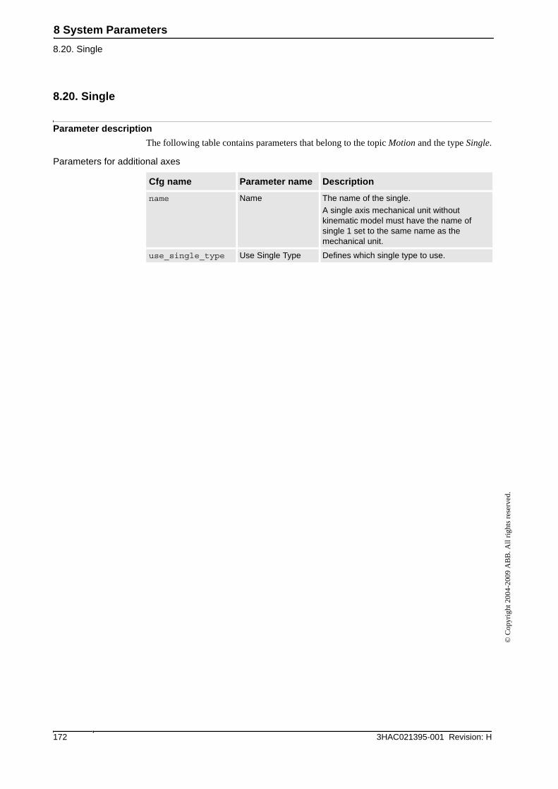
8 System Parameters
8.20. Single
3HAC021395-001 Revision: H172
© C
opyr
ight
200
4-20
09 A
BB
. All
righ
ts r
eser
ved.
8.20. Single
Parameter description
The following table contains parameters that belong to the topic Motion and the type Single.
Parameters for additional axes
Cfg name Parameter name Description
name Name The name of the single.
A single axis mechanical unit without kinematic model must have the name of single 1 set to the same name as the mechanical unit.
use_single_type Use Single Type Defines which single type to use.
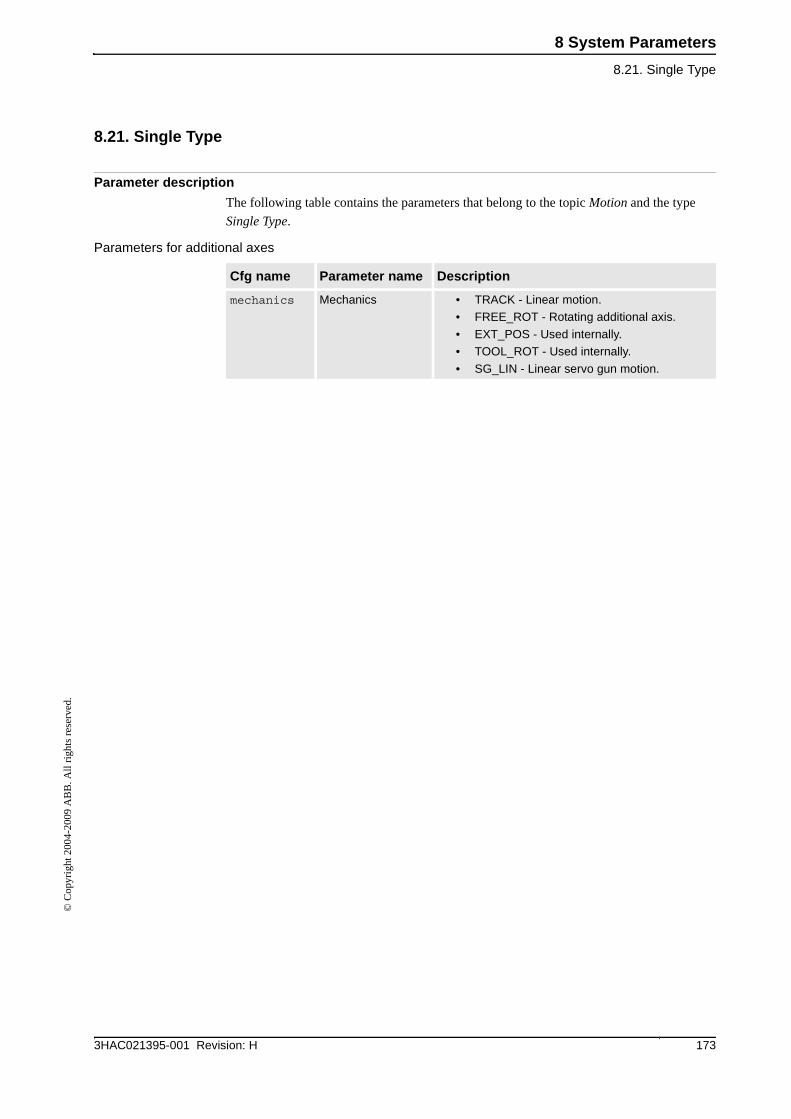
8 System Parameters
8.21. Single Type
1733HAC021395-001 Revision: H
© C
opyr
ight
200
4-20
09 A
BB
. All
righ
ts r
eser
ved.
8.21. Single Type
Parameter description
The following table contains the parameters that belong to the topic Motion and the type
Single Type.
Parameters for additional axes
Cfg name Parameter name Description
mechanics Mechanics • TRACK - Linear motion.
• FREE_ROT - Rotating additional axis.
• EXT_POS - Used internally.
• TOOL_ROT - Used internally.
• SG_LIN - Linear servo gun motion.
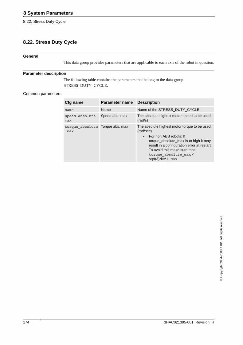
8 System Parameters
8.22. Stress Duty Cycle
3HAC021395-001 Revision: H174
© C
opyr
ight
200
4-20
09 A
BB
. All
righ
ts r
eser
ved.
8.22. Stress Duty Cycle
General
This data group provides parameters that are applicable to each axis of the robot in question.
Parameter description
The following table contains the parameters that belong to the data group
STRESS_DUTY_CYCLE.
Common parameters
Cfg name Parameter name Description
name Name Name of the STRESS_DUTY_CYCLE.
speed_absolute_max
Speed abs. max The absolute highest motor speed to be used. (rad/s)
torque_absolute_max
Torque abs. max The absolute highest motor torque to be used. (rad/sec)
• For non ABB robots: If torque_absolute_max is to high it may result in a configuration error at restart. To avoid this make sure that: torque_absolute_max < sqrt(3)*ke*i_max.
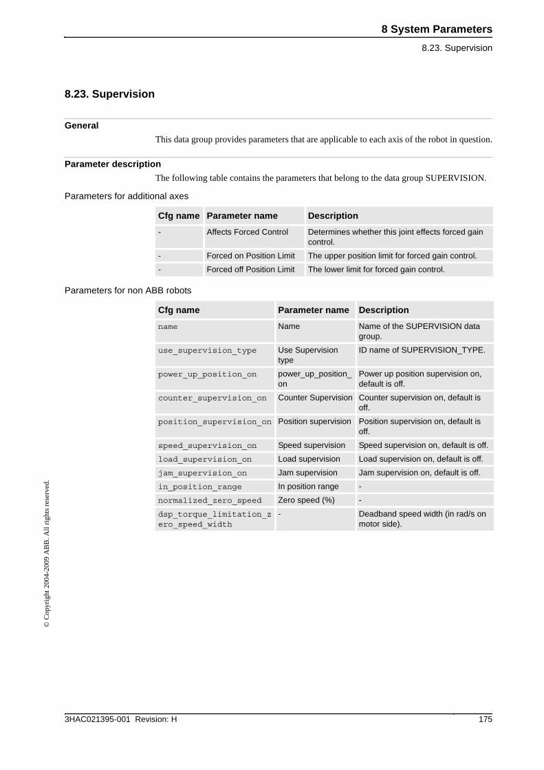
8 System Parameters
8.23. Supervision
1753HAC021395-001 Revision: H
© C
opyr
ight
200
4-20
09 A
BB
. All
righ
ts r
eser
ved.
8.23. Supervision
General
This data group provides parameters that are applicable to each axis of the robot in question.
Parameter description
The following table contains the parameters that belong to the data group SUPERVISION.
Parameters for additional axes
Parameters for non ABB robots
Cfg name Parameter name Description
- Affects Forced Control Determines whether this joint effects forced gain control.
- Forced on Position Limit The upper position limit for forced gain control.
- Forced off Position Limit The lower limit for forced gain control.
Cfg name Parameter name Description
name Name Name of the SUPERVISION data group.
use_supervision_type Use Supervision type
ID name of SUPERVISION_TYPE.
power_up_position_on power_up_position_on
Power up position supervision on, default is off.
counter_supervision_on Counter Supervision Counter supervision on, default is off.
position_supervision_on Position supervision Position supervision on, default is off.
speed_supervision_on Speed supervision Speed supervision on, default is off.
load_supervision_on Load supervision Load supervision on, default is off.
jam_supervision_on Jam supervision Jam supervision on, default is off.
in_position_range In position range -
normalized_zero_speed Zero speed (%) -
dsp_torque_limitation_zero_speed_width
- Deadband speed width (in rad/s on motor side).
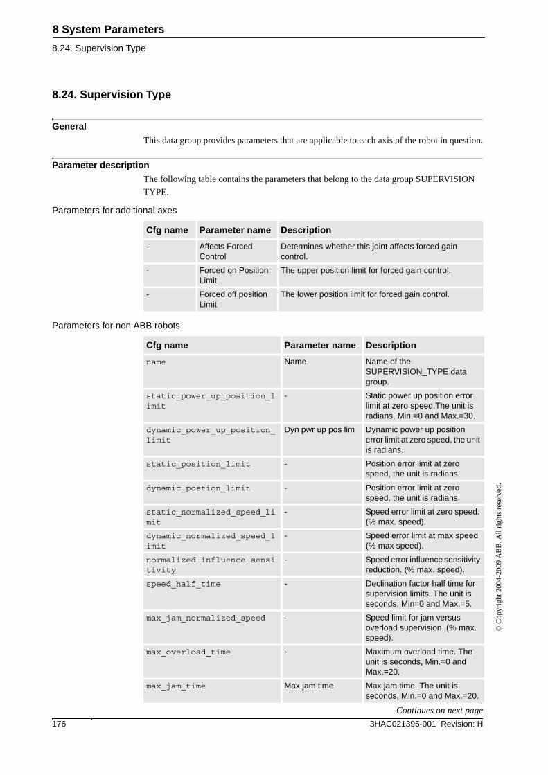
8 System Parameters
8.24. Supervision Type
3HAC021395-001 Revision: H176
© C
opyr
ight
200
4-20
09 A
BB
. All
righ
ts r
eser
ved.
8.24. Supervision Type
General
This data group provides parameters that are applicable to each axis of the robot in question.
Parameter description
The following table contains the parameters that belong to the data group SUPERVISION
TYPE.
Parameters for additional axes
Parameters for non ABB robots
Cfg name Parameter name Description
- Affects Forced Control
Determines whether this joint affects forced gain control.
- Forced on Position Limit
The upper position limit for forced gain control.
- Forced off position Limit
The lower position limit for forced gain control.
Cfg name Parameter name Description
name Name Name of the SUPERVISION_TYPE data group.
static_power_up_position_limit
- Static power up position error limit at zero speed.The unit is radians, Min.=0 and Max.=30.
dynamic_power_up_position_limit
Dyn pwr up pos lim Dynamic power up position error limit at zero speed, the unit is radians.
static_position_limit - Position error limit at zero speed, the unit is radians.
dynamic_postion_limit - Position error limit at zero speed, the unit is radians.
static_normalized_speed_limit
- Speed error limit at zero speed. (% max. speed).
dynamic_normalized_speed_limit
- Speed error limit at max speed (% max speed).
normalized_influence_sensitivity
- Speed error influence sensitivity reduction. (% max. speed).
speed_half_time - Declination factor half time for supervision limits. The unit is seconds, Min=0 and Max.=5.
max_jam_normalized_speed - Speed limit for jam versus overload supervision. (% max. speed).
max_overload_time - Maximum overload time. The unit is seconds, Min.=0 and Max.=20.
max_jam_time Max jam time Max jam time. The unit is seconds, Min.=0 and Max.=20.
Continues on next page
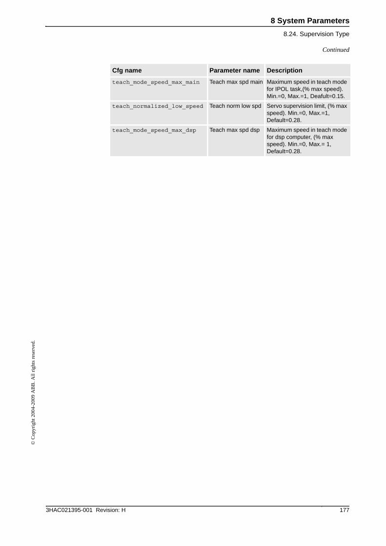
8 System Parameters
8.24. Supervision Type
1773HAC021395-001 Revision: H
© C
opyr
ight
200
4-20
09 A
BB
. All
righ
ts r
eser
ved.
teach_mode_speed_max_main Teach max spd main Maximum speed in teach mode for IPOL task,(% max speed). Min.=0, Max.=1, Deafult=0.15.
teach_normalized_low_speed Teach norm low spd Servo supervision limit, (% max speed). Min.=0, Max.=1, Default=0.28.
teach_mode_speed_max_dsp Teach max spd dsp Maximum speed in teach mode for dsp computer, (% max speed). Min.=0, Max.= 1, Default=0.28.
Cfg name Parameter name Description
Continued
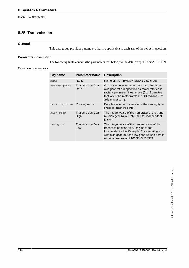
8 System Parameters
8.25. Transmission
3HAC021395-001 Revision: H178
© C
opyr
ight
200
4-20
09 A
BB
. All
righ
ts r
eser
ved.
8.25. Transmission
General
This data group provides parameters that are applicable to each arm of the robot in question.
Parameter description
The following table contains the parameters that belong to the data group TRANSMISSION.
Common parameters
Cfg name Parameter name Description
name Name Name off the TRANSMISSION data group.
transm_joint Transmission Gear Ratio
Gear ratio between motor and axis. For linear axis gear ratio is specified as motor rotation in radians per meter linear move (21.43 denotes that when the motor rotates 21.43 radians - the axis moves 1 m).
rotating_move Rotating move Denotes whether the axis is of the rotating type (Yes) or linear type (No).
high_gear Transmission Gear High
The integer value of the numerator of the trans-mission gear ratio. Only used for independent joints.
low_gear Transmission Gear Low
The integer value of the denominators of the transmission gear ratio. Only used for independent joints.Example: For a rotating axis with high gear 100 and low gear 30, has a trans-mission gear ratio of 100/30=3.333333.
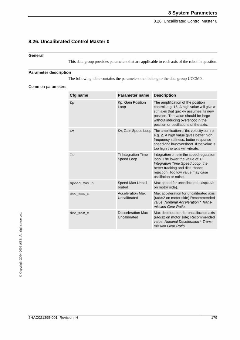
8 System Parameters
8.26. Uncalibrated Control Master 0
1793HAC021395-001 Revision: H
© C
opyr
ight
200
4-20
09 A
BB
. All
righ
ts r
eser
ved.
8.26. Uncalibrated Control Master 0
General
This data group provides parameters that are applicable to each axis of the robot in question.
Parameter description
The following table contains the parameters that belong to the data group UCCM0.
Common parameters
Cfg name Parameter name Description
Kp Kp, Gain Position Loop
The amplification of the position control, e.g. 15. A high value will give a stiff axis that quickly assumes its new position. The value should be large without inducing overshoot in the position or oscillations of the axis.
Kv Kv, Gain Speed Loop The amplification of the velocity control, e.g. 2. A high value gives better high frequency stiffness, better response speed and low overshoot. If the value is too high the axis will vibrate.
Ti Ti Integration Time Speed Loop
Integration time in the speed regulation loop. The lower the value of Ti Integration Time Speed Loop, the better tracking and disturbance rejection. Too low value may case oscillation or noise.
speed_max_n Speed Max Uncali-brated
Max speed for uncalibrated axis(rad/s on motor side).
acc_max_n Acceleration Max Uncalibrated
Max acceleration for uncalibrated axis (rad/s2 on motor side) Recommended value: Nominal Acceleration * Trans-mission Gear Ratio.
dec_max_n Decceleration Max Uncalibrated
Max deceleration for uncalibrated axis (rad/s2 on motor side) Recommended value: Nominal Deceleration * Trans-mission Gear Ratio.

8 System Parameters
8.26. Uncalibrated Control Master 0
3HAC021395-001 Revision: H180
© C
opyr
ight
200
4-20
09 A
BB
. All
righ
ts r
eser
ved.
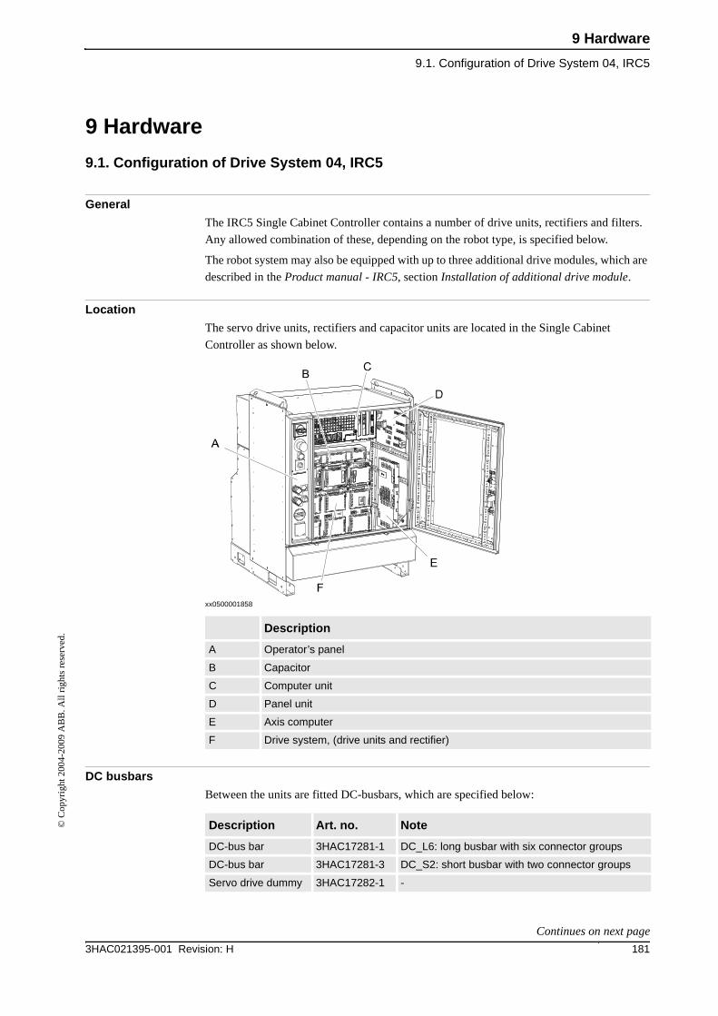
9 Hardware
9.1. Configuration of Drive System 04, IRC5
1813HAC021395-001 Revision: H
© C
opyr
ight
200
4-20
09 A
BB
. All
righ
ts r
eser
ved.
9 Hardware
9.1. Configuration of Drive System 04, IRC5
General
The IRC5 Single Cabinet Controller contains a number of drive units, rectifiers and filters.
Any allowed combination of these, depending on the robot type, is specified below.
The robot system may also be equipped with up to three additional drive modules, which are
described in the Product manual - IRC5, section Installation of additional drive module.
Location
The servo drive units, rectifiers and capacitor units are located in the Single Cabinet
Controller as shown below.
xx0500001858
DC busbars
Between the units are fitted DC-busbars, which are specified below:
Description
A Operator’s panel
B Capacitor
C Computer unit
D Panel unit
E Axis computer
F Drive system, (drive units and rectifier)
Description Art. no. Note
DC-bus bar 3HAC17281-1 DC_L6: long busbar with six connector groups
DC-bus bar 3HAC17281-3 DC_S2: short busbar with two connector groups
Servo drive dummy 3HAC17282-1 -
Continues on next page
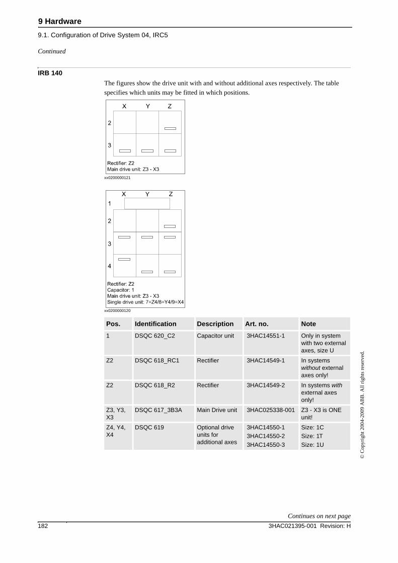
9 Hardware
9.1. Configuration of Drive System 04, IRC5
3HAC021395-001 Revision: H182
© C
opyr
ight
200
4-20
09 A
BB
. All
righ
ts r
eser
ved.
IRB 140
The figures show the drive unit with and without additional axes respectively. The table
specifies which units may be fitted in which positions.
xx0200000121
xx0200000120
Pos. Identification Description Art. no. Note
1 DSQC 620_C2 Capacitor unit 3HAC14551-1 Only in system with two external axes, size U
Z2 DSQC 618_RC1 Rectifier 3HAC14549-1 In systems without external axes only!
Z2 DSQC 618_R2 Rectifier 3HAC14549-2 In systems with external axes only!
Z3, Y3, X3
DSQC 617_3B3A Main Drive unit 3HAC025338-001 Z3 - X3 is ONE unit!
Z4, Y4, X4
DSQC 619 Optional drive units for additional axes
3HAC14550-1
3HAC14550-2
3HAC14550-3
Size: 1C
Size: 1T
Size: 1U
Continued
Continues on next page
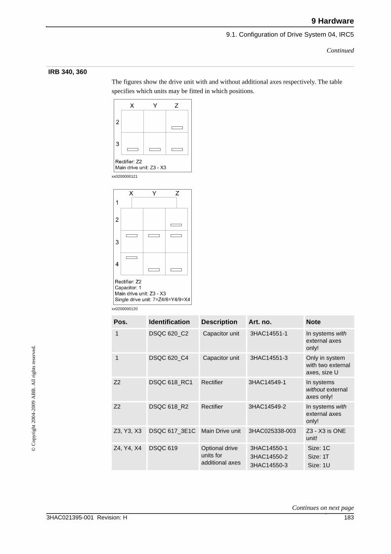
9 Hardware
9.1. Configuration of Drive System 04, IRC5
1833HAC021395-001 Revision: H
© C
opyr
ight
200
4-20
09 A
BB
. All
righ
ts r
eser
ved.
IRB 340, 360
The figures show the drive unit with and without additional axes respectively. The table
specifies which units may be fitted in which positions.
xx0200000121
xx0200000120
Pos. Identification Description Art. no. Note
1 DSQC 620_C2 Capacitor unit 3HAC14551-1 In systems with external axes only!
1 DSQC 620_C4 Capacitor unit 3HAC14551-3 Only in system with two external axes, size U
Z2 DSQC 618_RC1 Rectifier 3HAC14549-1 In systems without external axes only!
Z2 DSQC 618_R2 Rectifier 3HAC14549-2 In systems with external axes only!
Z3, Y3, X3 DSQC 617_3E1C Main Drive unit 3HAC025338-003 Z3 - X3 is ONE unit!
Z4, Y4, X4 DSQC 619 Optional drive units for additional axes
3HAC14550-1
3HAC14550-2
3HAC14550-3
Size: 1C
Size: 1T
Size: 1U
Continued
Continues on next page
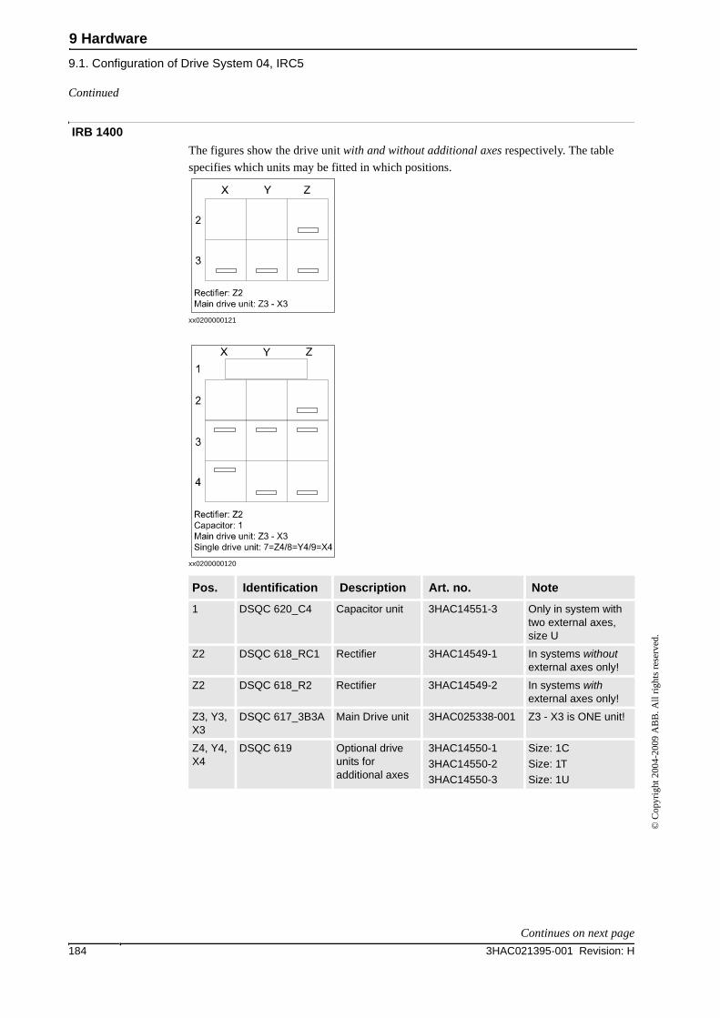
9 Hardware
9.1. Configuration of Drive System 04, IRC5
3HAC021395-001 Revision: H184
© C
opyr
ight
200
4-20
09 A
BB
. All
righ
ts r
eser
ved.
IRB 1400
The figures show the drive unit with and without additional axes respectively. The table
specifies which units may be fitted in which positions.
xx0200000121
xx0200000120
Pos. Identification Description Art. no. Note
1 DSQC 620_C4 Capacitor unit 3HAC14551-3 Only in system with two external axes, size U
Z2 DSQC 618_RC1 Rectifier 3HAC14549-1 In systems without external axes only!
Z2 DSQC 618_R2 Rectifier 3HAC14549-2 In systems with external axes only!
Z3, Y3, X3
DSQC 617_3B3A Main Drive unit 3HAC025338-001 Z3 - X3 is ONE unit!
Z4, Y4, X4
DSQC 619 Optional drive units for additional axes
3HAC14550-1
3HAC14550-2
3HAC14550-3
Size: 1C
Size: 1T
Size: 1U
Continued
Continues on next page
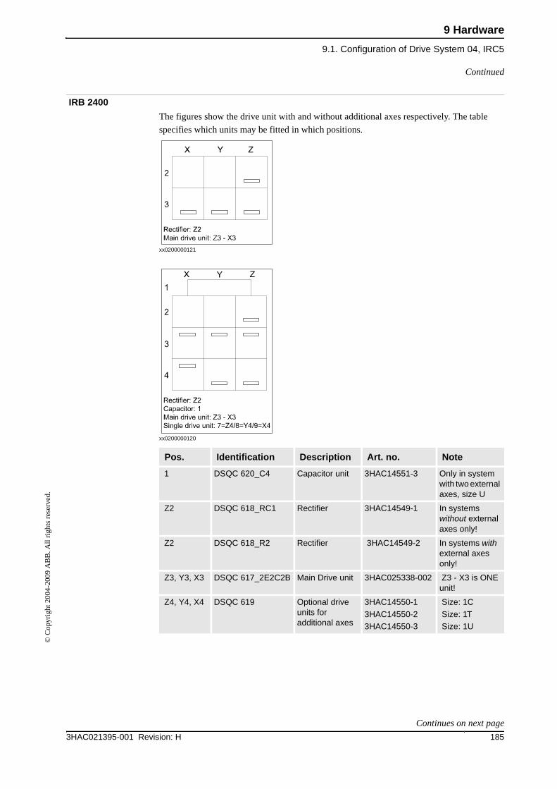
9 Hardware
9.1. Configuration of Drive System 04, IRC5
1853HAC021395-001 Revision: H
© C
opyr
ight
200
4-20
09 A
BB
. All
righ
ts r
eser
ved.
IRB 2400
The figures show the drive unit with and without additional axes respectively. The table
specifies which units may be fitted in which positions.
xx0200000121
xx0200000120
Pos. Identification Description Art. no. Note
1 DSQC 620_C4 Capacitor unit 3HAC14551-3 Only in system with two external axes, size U
Z2 DSQC 618_RC1 Rectifier 3HAC14549-1 In systems without external axes only!
Z2 DSQC 618_R2 Rectifier 3HAC14549-2 In systems with external axes only!
Z3, Y3, X3 DSQC 617_2E2C2B Main Drive unit 3HAC025338-002 Z3 - X3 is ONE unit!
Z4, Y4, X4 DSQC 619 Optional drive units for additional axes
3HAC14550-1
3HAC14550-2
3HAC14550-3
Size: 1C
Size: 1T
Size: 1U
Continued
Continues on next page
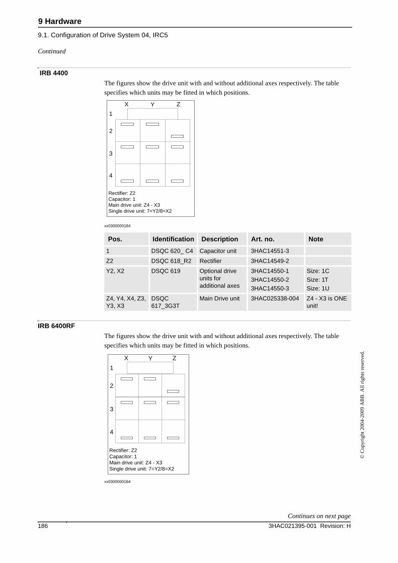
9 Hardware
9.1. Configuration of Drive System 04, IRC5
3HAC021395-001 Revision: H186
© C
opyr
ight
200
4-20
09 A
BB
. All
righ
ts r
eser
ved.
IRB 4400
The figures show the drive unit with and without additional axes respectively. The table
specifies which units may be fitted in which positions.
xx0300000184
IRB 6400RF
The figures show the drive unit with and without additional axes respectively. The table
specifies which units may be fitted in which positions.
xx0300000184
Pos. Identification Description Art. no. Note
1 DSQC 620_ C4 Capacitor unit 3HAC14551-3
Z2 DSQC 618_R2 Rectifier 3HAC14549-2
Y2, X2 DSQC 619 Optional drive units for additional axes
3HAC14550-1
3HAC14550-2
3HAC14550-3
Size: 1C
Size: 1T
Size: 1U
Z4, Y4, X4, Z3, Y3, X3
DSQC 617_3G3T
Main Drive unit 3HAC025338-004 Z4 - X3 is ONE unit!
1
2
3
4
ZYX
Rectifier: Z2Capacitor: 1Main drive unit: Z4 - X3Single drive unit: 7=Y2/8=X2
1
2
3
4
ZYX
Rectifier: Z2Capacitor: 1Main drive unit: Z4 - X3Single drive unit: 7=Y2/8=X2
Continued
Continues on next page
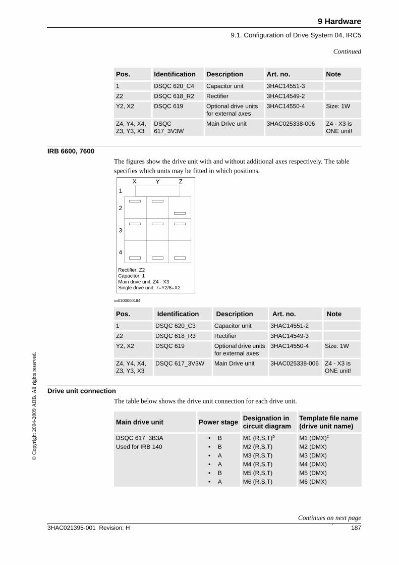
9 Hardware
9.1. Configuration of Drive System 04, IRC5
1873HAC021395-001 Revision: H
© C
opyr
ight
200
4-20
09 A
BB
. All
righ
ts r
eser
ved.
IRB 6600, 7600
The figures show the drive unit with and without additional axes respectively. The table
specifies which units may be fitted in which positions.
xx0300000184
Drive unit connection
The table below shows the drive unit connection for each drive unit.
Pos. Identification Description Art. no. Note
1 DSQC 620_C4 Capacitor unit 3HAC14551-3
Z2 DSQC 618_R2 Rectifier 3HAC14549-2
Y2, X2 DSQC 619 Optional drive units for external axes
3HAC14550-4 Size: 1W
Z4, Y4, X4, Z3, Y3, X3
DSQC 617_3V3W
Main Drive unit 3HAC025338-006 Z4 - X3 is ONE unit!
Pos. Identification Description Art. no. Note
1 DSQC 620_C3 Capacitor unit 3HAC14551-2
Z2 DSQC 618_R3 Rectifier 3HAC14549-3
Y2, X2 DSQC 619 Optional drive units for external axes
3HAC14550-4 Size: 1W
Z4, Y4, X4, Z3, Y3, X3
DSQC 617_3V3W Main Drive unit 3HAC025338-006 Z4 - X3 is ONE unit!
1
2
3
4
ZYX
Rectifier: Z2Capacitor: 1Main drive unit: Z4 - X3Single drive unit: 7=Y2/8=X2
Main drive unit Power stageDesignation in circuit diagram
Template file name (drive unit name)
DSQC 617_3B3A
Used for IRB 140
• B
• B
• A
• A
• B
• A
M1 (R,S,T)b
M2 (R,S,T)
M3 (R,S,T)
M4 (R,S,T)
M5 (R,S,T)
M6 (R,S,T)
M1 (DMX)c
M2 (DMX)
M3 (DMX)
M4 (DMX)
M5 (DMX)
M6 (DMX)
Continued
Continues on next page
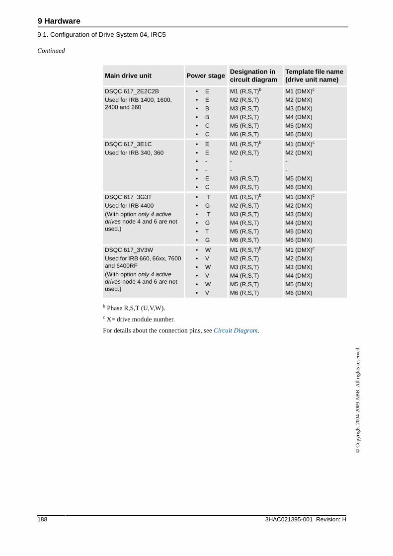
9 Hardware
9.1. Configuration of Drive System 04, IRC5
3HAC021395-001 Revision: H188
© C
opyr
ight
200
4-20
09 A
BB
. All
righ
ts r
eser
ved.
b Phase R,S,T (U,V,W).c X= drive module number.
For details about the connection pins, see Circuit Diagram.
DSQC 617_2E2C2B
Used for IRB 1400, 1600, 2400 and 260
• E
• E
• B
• B
• C
• C
M1 (R,S,T)b
M2 (R,S,T)
M3 (R,S,T)
M4 (R,S,T)
M5 (R,S,T)
M6 (R,S,T)
M1 (DMX)c
M2 (DMX)
M3 (DMX)
M4 (DMX)
M5 (DMX)
M6 (DMX)
DSQC 617_3E1C
Used for IRB 340, 360
• E
• E
• -
• -
• E
• C
M1 (R,S,T)b
M2 (R,S,T)
-
-
M3 (R,S,T)
M4 (R,S,T)
M1 (DMX)c
M2 (DMX)
-
-
M5 (DMX)
M6 (DMX)
DSQC 617_3G3T
Used for IRB 4400
(With option only 4 active drives node 4 and 6 are not used.)
• T
• G
• T
• G
• T
• G
M1 (R,S,T)b
M2 (R,S,T)
M3 (R,S,T)
M4 (R,S,T)
M5 (R,S,T)
M6 (R,S,T)
M1 (DMX)c
M2 (DMX)
M3 (DMX)
M4 (DMX)
M5 (DMX)
M6 (DMX)
DSQC 617_3V3W
Used for IRB 660, 66xx, 7600 and 6400RF
(With option only 4 active drives node 4 and 6 are not used.)
• W
• V
• W
• V
• W
• V
M1 (R,S,T)b
M2 (R,S,T)
M3 (R,S,T)
M4 (R,S,T)
M5 (R,S,T)
M6 (R,S,T)
M1 (DMX)c
M2 (DMX)
M3 (DMX)
M4 (DMX)
M5 (DMX)
M6 (DMX)
Main drive unit Power stageDesignation in circuit diagram
Template file name (drive unit name)
Continued
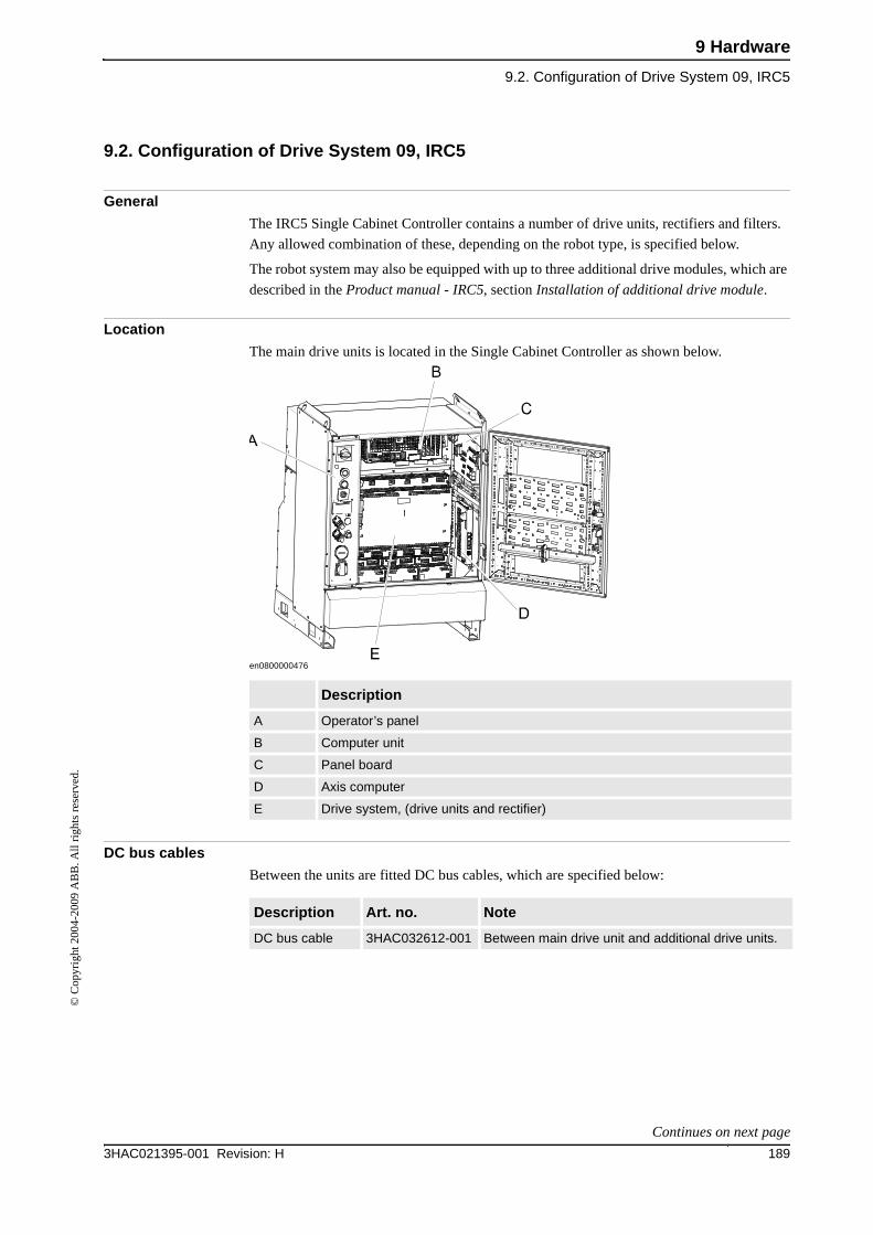
9 Hardware
9.2. Configuration of Drive System 09, IRC5
1893HAC021395-001 Revision: H
© C
opyr
ight
200
4-20
09 A
BB
. All
righ
ts r
eser
ved.
9.2. Configuration of Drive System 09, IRC5
General
The IRC5 Single Cabinet Controller contains a number of drive units, rectifiers and filters.
Any allowed combination of these, depending on the robot type, is specified below.
The robot system may also be equipped with up to three additional drive modules, which are
described in the Product manual - IRC5, section Installation of additional drive module.
Location
The main drive units is located in the Single Cabinet Controller as shown below.
en0800000476
DC bus cables
Between the units are fitted DC bus cables, which are specified below:
Description
A Operator’s panel
B Computer unit
C Panel board
D Axis computer
E Drive system, (drive units and rectifier)
Description Art. no. Note
DC bus cable 3HAC032612-001 Between main drive unit and additional drive units.
Continues on next page
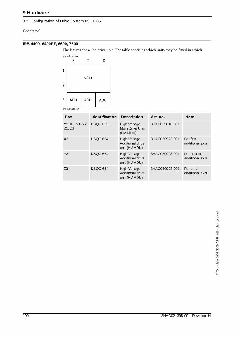
9 Hardware
9.2. Configuration of Drive System 09, IRC5
3HAC021395-001 Revision: H190
© C
opyr
ight
200
4-20
09 A
BB
. All
righ
ts r
eser
ved.
IRB 4400, 6400RF, 6600, 7600
The figures show the drive unit. The table specifies which units may be fitted in which
positions.
en0800000292
Pos. Identification Description Art. no. Note
Y1, X2, Y1, Y2, Z1, Z2
DSQC 663 High Voltage Main Drive Unit (HV MDU)
3HAC029818-001
X3 DSQC 664 High Voltage Additional drive unit (HV ADU)
3HAC030923-001 For first additional axis
Y3 DSQC 664 High Voltage Additional drive unit (HV ADU)
3HAC030923-001 For second additional axis
Z3 DSQC 664 High Voltage Additional drive unit (HV ADU)
3HAC030923-001 For third additional axis
Continued

9 Hardware
9.3. Transformers
1913HAC021395-001 Revision: H
© C
opyr
ight
200
4-20
09 A
BB
. All
righ
ts r
eser
ved.
9.3. Transformers
Overview
The transformer is used to transform the incoming voltage to the voltage used in the cabinet.
The selection of transformer depends on the selection of primary voltage and drive units.
Voltage alternative
The transformers are reversible to following primary voltage alternatives.
• 200 V
• 220 V
• 400 V
• 440 V
• 480 V
• 500 V
• 600 V
Technical data
The following table details the standard option transformers.
Robot type Primary voltage (V) Effect (kVA)
140, 260, 340,
1410, 1600, 2400,
4400, 6400RF
200-600 V 6 kVA
66xx, 7600 < 400 V
480 V
> 480 V
13 kVA
1.8 kVA, for electronics
13 kVA
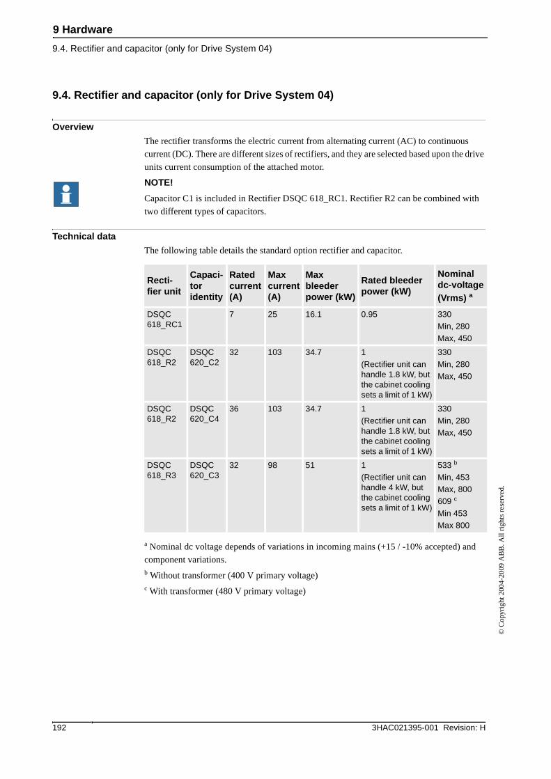
9 Hardware
9.4. Rectifier and capacitor (only for Drive System 04)
3HAC021395-001 Revision: H192
© C
opyr
ight
200
4-20
09 A
BB
. All
righ
ts r
eser
ved.
9.4. Rectifier and capacitor (only for Drive System 04)
Overview
The rectifier transforms the electric current from alternating current (AC) to continuous
current (DC). There are different sizes of rectifiers, and they are selected based upon the drive
units current consumption of the attached motor.
NOTE!
Capacitor C1 is included in Rectifier DSQC 618_RC1. Rectifier R2 can be combined with
two different types of capacitors.
Technical data
The following table details the standard option rectifier and capacitor.
a Nominal dc voltage depends of variations in incoming mains (+15 / -10% accepted) and
component variations.b Without transformer (400 V primary voltage)c With transformer (480 V primary voltage)
Recti-fier unit
Capaci-tor identity
Rated current (A)
Max current (A)
Max bleeder power (kW)
Rated bleeder power (kW)
Nominal dc-voltage (Vrms) a
DSQC 618_RC1
7 25 16.1 0.95 330
Min, 280
Max, 450
DSQC 618_R2
DSQC 620_C2
32 103 34.7 1
(Rectifier unit can handle 1.8 kW, but the cabinet cooling sets a limit of 1 kW)
330
Min, 280
Max, 450
DSQC 618_R2
DSQC 620_C4
36 103 34.7 1
(Rectifier unit can handle 1.8 kW, but the cabinet cooling sets a limit of 1 kW)
330
Min, 280
Max, 450
DSQC 618_R3
DSQC 620_C3
32 98 51 1
(Rectifier unit can handle 4 kW, but the cabinet cooling sets a limit of 1 kW)
533 b
Min, 453
Max, 800
609 c
Min 453
Max 800
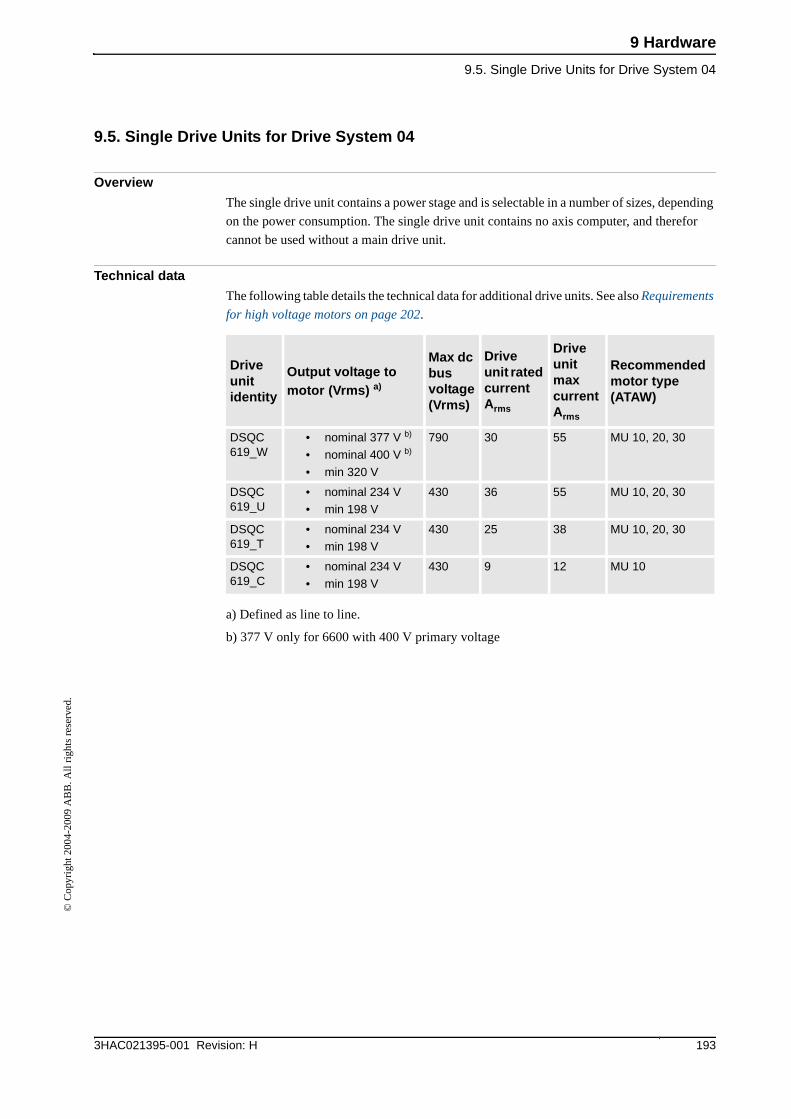
9 Hardware
9.5. Single Drive Units for Drive System 04
1933HAC021395-001 Revision: H
© C
opyr
ight
200
4-20
09 A
BB
. All
righ
ts r
eser
ved.
9.5. Single Drive Units for Drive System 04
Overview
The single drive unit contains a power stage and is selectable in a number of sizes, depending
on the power consumption. The single drive unit contains no axis computer, and therefor
cannot be used without a main drive unit.
Technical data
The following table details the technical data for additional drive units. See also Requirements
for high voltage motors on page 202.
a) Defined as line to line.
b) 377 V only for 6600 with 400 V primary voltage
Drive unit identity
Output voltage to motor (Vrms) a)
Max dc bus voltage (Vrms)
Drive unit rated current Arms
Drive unit max current Arms
Recommended motor type (ATAW)
DSQC 619_W
• nominal 377 V b)
• nominal 400 V b)
• min 320 V
790 30 55 MU 10, 20, 30
DSQC 619_U
• nominal 234 V
• min 198 V
430 36 55 MU 10, 20, 30
DSQC 619_T
• nominal 234 V
• min 198 V
430 25 38 MU 10, 20, 30
DSQC 619_C
• nominal 234 V
• min 198 V
430 9 12 MU 10
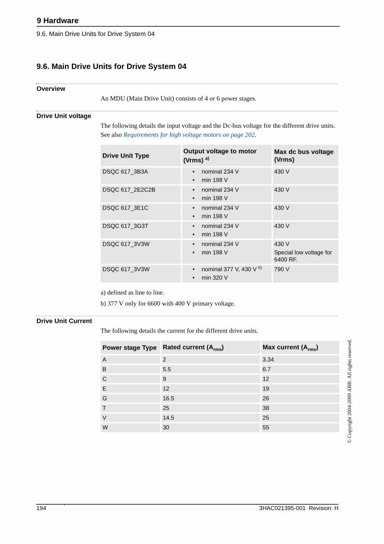
9 Hardware
9.6. Main Drive Units for Drive System 04
3HAC021395-001 Revision: H194
© C
opyr
ight
200
4-20
09 A
BB
. All
righ
ts r
eser
ved.
9.6. Main Drive Units for Drive System 04
Overview
An MDU (Main Drive Unit) consists of 4 or 6 power stages.
Drive Unit voltage
The following details the input voltage and the Dc-bus voltage for the different drive units.
See also Requirements for high voltage motors on page 202.
a) defined as line to line.
b) 377 V only for 6600 with 400 V primary voltage.
Drive Unit Current
The following details the current for the different drive units.
Drive Unit TypeOutput voltage to motor (Vrms) a)
Max dc bus voltage (Vrms)
DSQC 617_3B3A • nominal 234 V
• min 198 V
430 V
DSQC 617_2E2C2B • nominal 234 V
• min 198 V
430 V
DSQC 617_3E1C • nominal 234 V
• min 198 V
430 V
DSQC 617_3G3T • nominal 234 V
• min 198 V
430 V
DSQC 617_3V3W • nominal 234 V
• min 198 V
430 V
Special low voltage for 6400 RF.
DSQC 617_3V3W • nominal 377 V, 430 V b)
• min 320 V
790 V
Power stage Type Rated current (Arms) Max current (Arms)
A 2 3.34
B 5.5 6.7
C 9 12
E 12 19
G 16.5 26
T 25 38
V 14.5 25
W 30 55
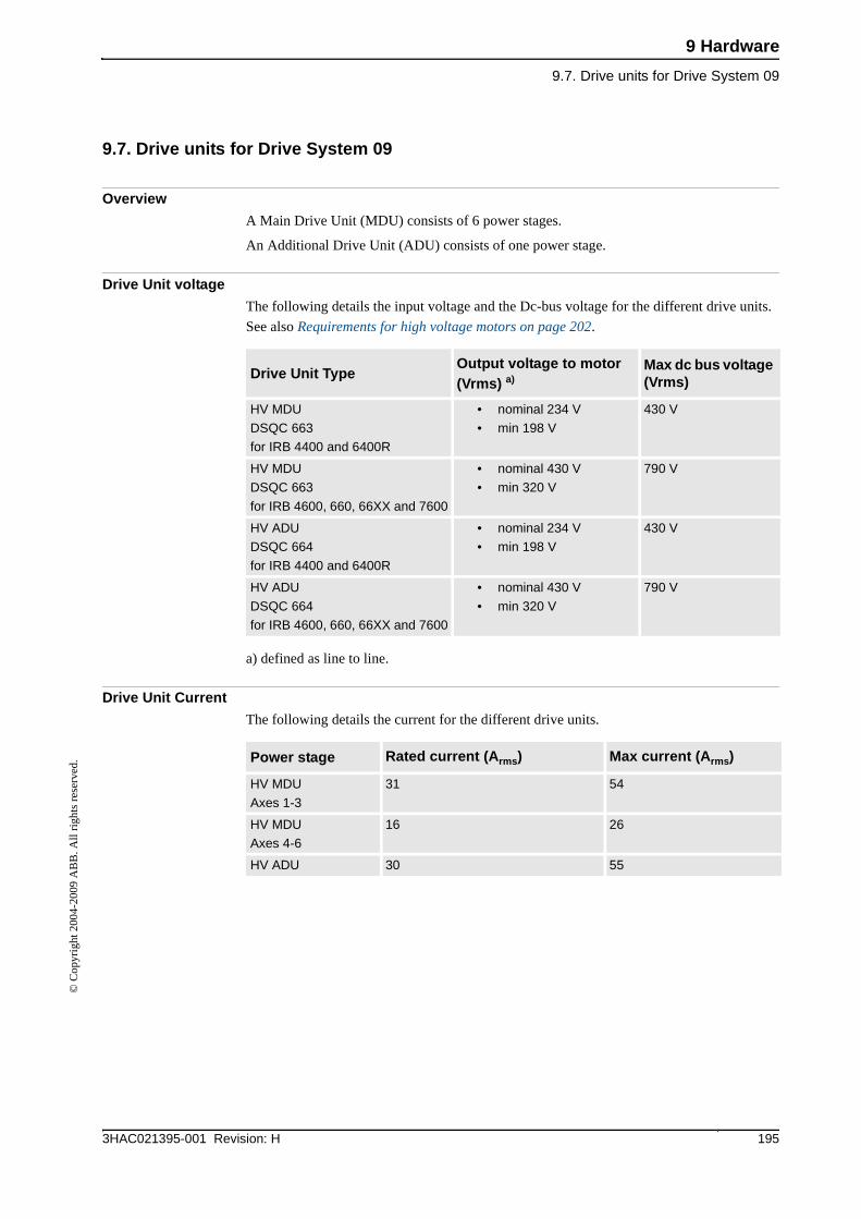
9 Hardware
9.7. Drive units for Drive System 09
1953HAC021395-001 Revision: H
© C
opyr
ight
200
4-20
09 A
BB
. All
righ
ts r
eser
ved.
9.7. Drive units for Drive System 09
Overview
A Main Drive Unit (MDU) consists of 6 power stages.
An Additional Drive Unit (ADU) consists of one power stage.
Drive Unit voltage
The following details the input voltage and the Dc-bus voltage for the different drive units.
See also Requirements for high voltage motors on page 202.
a) defined as line to line.
Drive Unit Current
The following details the current for the different drive units.
Drive Unit TypeOutput voltage to motor (Vrms) a)
Max dc bus voltage (Vrms)
HV MDU
DSQC 663for IRB 4400 and 6400R
• nominal 234 V
• min 198 V
430 V
HV MDU
DSQC 663
for IRB 4600, 660, 66XX and 7600
• nominal 430 V
• min 320 V
790 V
HV ADUDSQC 664
for IRB 4400 and 6400R
• nominal 234 V• min 198 V
430 V
HV ADU
DSQC 664for IRB 4600, 660, 66XX and 7600
• nominal 430 V
• min 320 V
790 V
Power stage Rated current (Arms) Max current (Arms)
HV MDU
Axes 1-3
31 54
HV MDU
Axes 4-6
16 26
HV ADU 30 55
9 Hardware
9.8. Measurement System
3HAC021395-001 Revision: H196
© C
opyr
ight
200
4-20
09 A
BB
. All
righ
ts r
eser
ved.
9.8. Measurement System
Overview
This system can control up to nine axes at the same time, and measure another five axes.
Axes Computer Board
The drive module is equipped with one axes computer board which is connected to a
connector in the front of the cabinet.
Serial measurement links
Each drive module has two serial measurement links for measurement boards. The
connectors in the front of the drive module are marked, Measurement system 1 and
Measurement system 2. These serial links are ring circuits, which means that if there is more
than one board on the same link, the output from Serial Measurement Board 1 is connected
to the input on Serial Measurement Board 2. See Serial Measurement Link examples on
page 197.
Serial Measurement Board
The standard SMB has seven resolver inputs. These inputs can be used as seven different
nodes where the node number is equal to the axis number e.g. axis 1 to node 1.
Back-up battery
A back-up battery supplies the SMB with power during power failure. If an axis is moved
during power off, the system is ready for operation, and no synchronization is needed after
power on.
Features
Specifications for the measurement system:
• Each drive module can handle up to four SMBs divided on two serial links.
• Each serial link can handle up to seven axes.
• Each node 1 - 7 may only be used once on each link.
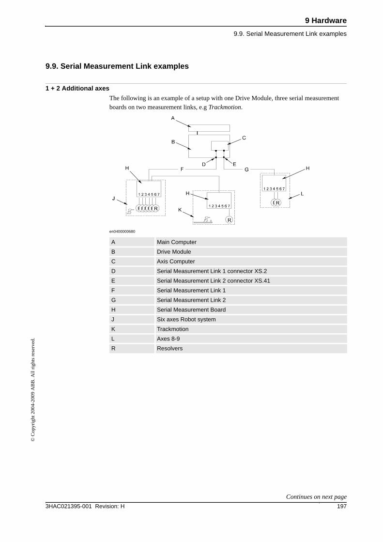
9 Hardware
9.9. Serial Measurement Link examples
1973HAC021395-001 Revision: H
© C
opyr
ight
200
4-20
09 A
BB
. All
righ
ts r
eser
ved.
9.9. Serial Measurement Link examples
1 + 2 Additional axes
The following is an example of a setup with one Drive Module, three serial measurement
boards on two measurement links, e.g Trackmotion.
en0400000680
A Main Computer
B Drive Module
C Axis Computer
D Serial Measurement Link 1 connector XS.2
E Serial Measurement Link 2 connector XS.41
F Serial Measurement Link 1
G Serial Measurement Link 2
H Serial Measurement Board
J Six axes Robot system
K Trackmotion
L Axes 8-9
R Resolvers
Continues on next page
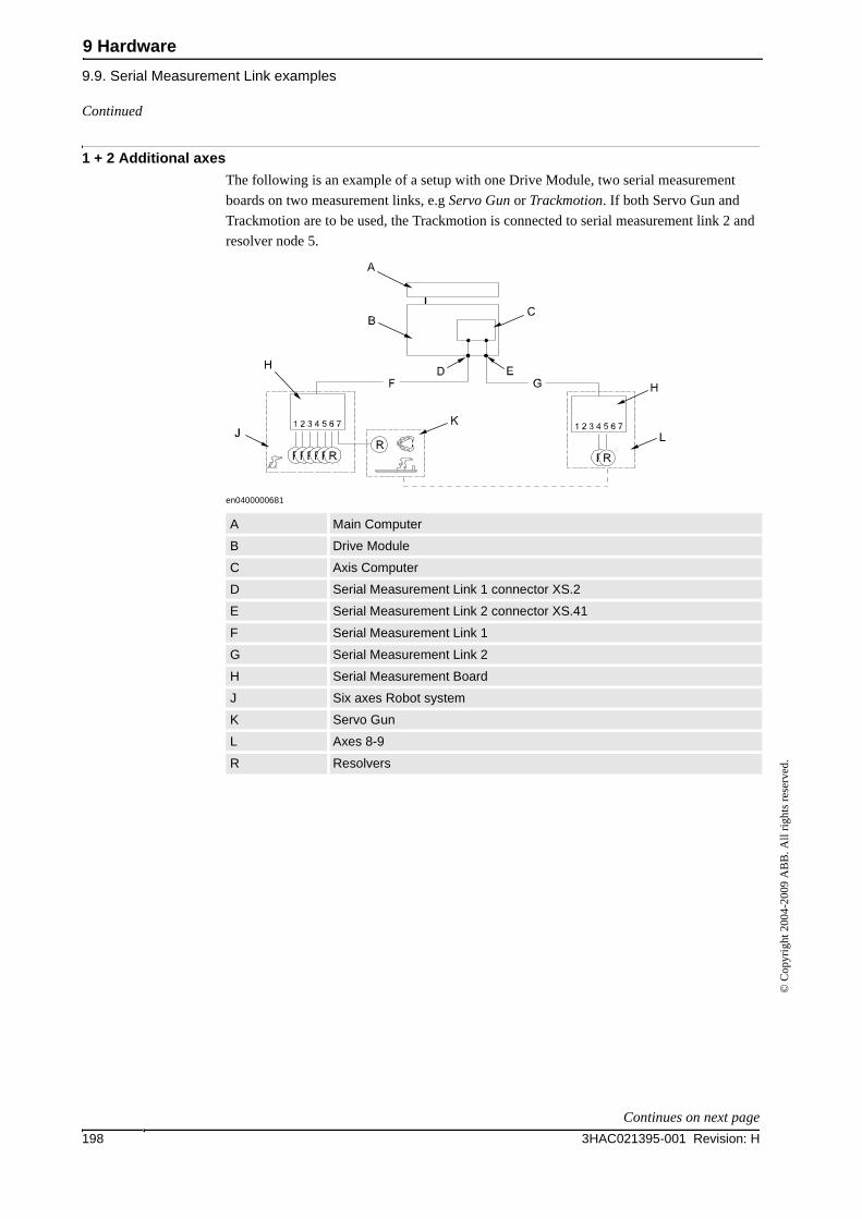
9 Hardware
9.9. Serial Measurement Link examples
3HAC021395-001 Revision: H198
© C
opyr
ight
200
4-20
09 A
BB
. All
righ
ts r
eser
ved.
1 + 2 Additional axes
The following is an example of a setup with one Drive Module, two serial measurement
boards on two measurement links, e.g Servo Gun or Trackmotion. If both Servo Gun and
Trackmotion are to be used, the Trackmotion is connected to serial measurement link 2 and
resolver node 5.
en0400000681
A Main Computer
B Drive Module
C Axis Computer
D Serial Measurement Link 1 connector XS.2
E Serial Measurement Link 2 connector XS.41
F Serial Measurement Link 1
G Serial Measurement Link 2
H Serial Measurement Board
J Six axes Robot system
K Servo Gun
L Axes 8-9
R Resolvers
Continued
Continues on next page
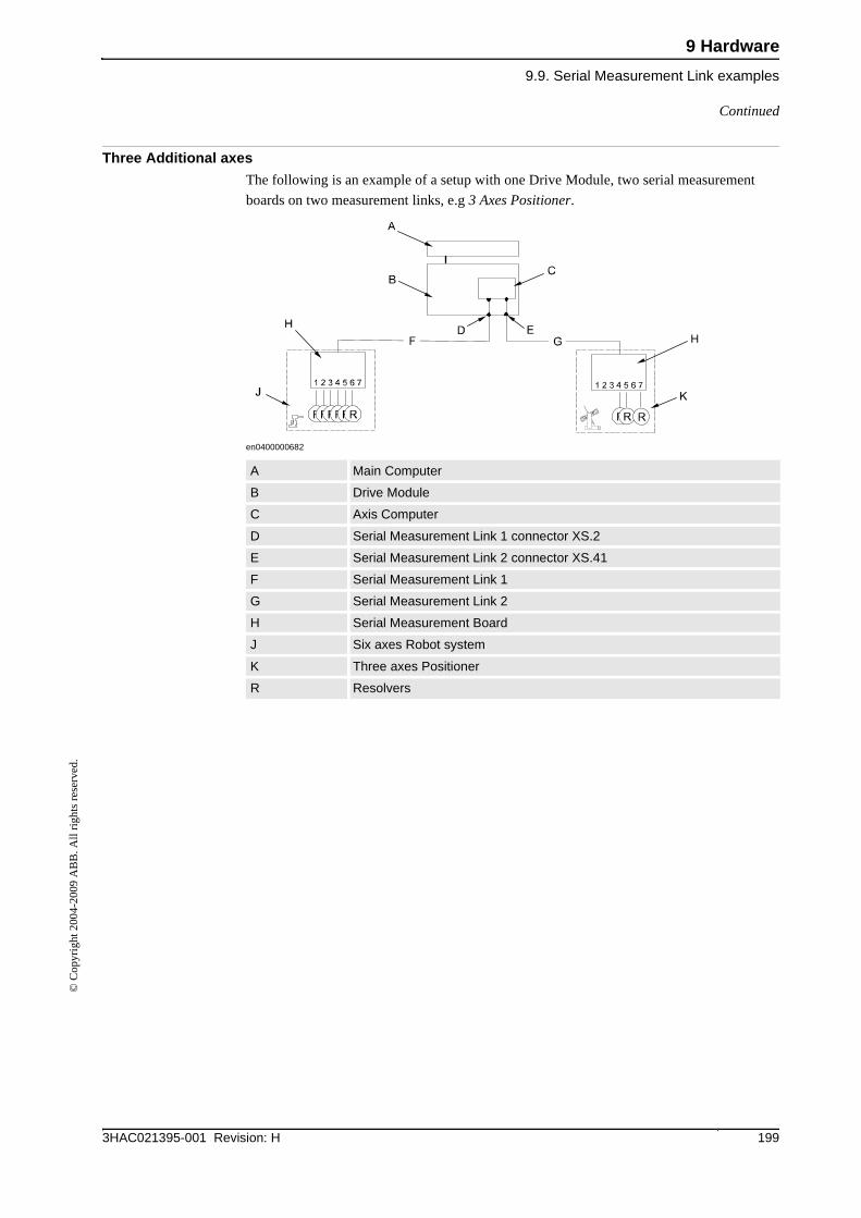
9 Hardware
9.9. Serial Measurement Link examples
1993HAC021395-001 Revision: H
© C
opyr
ight
200
4-20
09 A
BB
. All
righ
ts r
eser
ved.
Three Additional axes
The following is an example of a setup with one Drive Module, two serial measurement
boards on two measurement links, e.g 3 Axes Positioner.
en0400000682
A Main Computer
B Drive Module
C Axis Computer
D Serial Measurement Link 1 connector XS.2
E Serial Measurement Link 2 connector XS.41
F Serial Measurement Link 1
G Serial Measurement Link 2
H Serial Measurement Board
J Six axes Robot system
K Three axes Positioner
R Resolvers
Continued
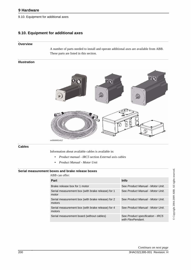
9 Hardware
9.10. Equipment for additional axes
3HAC021395-001 Revision: H200
© C
opyr
ight
200
4-20
09 A
BB
. All
righ
ts r
eser
ved.
9.10. Equipment for additional axes
Overview
A number of parts needed to install and operate additional axes are available from ABB.
These parts are listed in this section.
Illustration
xx0500001412
Cables
Information about available cables is available in:
• Product manual - IRC5 section External axis cables
• Product Manual - Motor Unit
Serial measurement boxes and brake release boxesABB can offer:
Part Info
Brake release box for 1 motor See Product Manual - Motor Unit.
Serial measurement box (with brake release) for 1 motor
See Product Manual - Motor Unit.
Serial measurement box (with brake release) for 2 motors
See Product Manual - Motor Unit.
Serial measurement box (with brake release) for 4 motors
See Product Manual - Motor Unit.
Serial measurement board (without cables) See Product specification - IRC5 with FlexPendant.
Continues on next page
9 Hardware
9.10. Equipment for additional axes
2013HAC021395-001 Revision: H
© C
opyr
ight
200
4-20
09 A
BB
. All
righ
ts r
eser
ved.
Motors, brakes and resolvers
ABB can offer motor unit kits specially designed for ABB's robots and can be used for
peripherals requiring servo-steered motors that are synchronized with the robot movements.
The motor units are designed for optimal performance and to facilitate installation and
application. These kits contain all the parts needed to install and operate additional motors.
The motor units are available in the following sizes:
For further information see Product Manual - Motor Unit.
Motor unit kit Max continuous torque Max motor speed
MU10 1.5 Nm 3300 rpm
MU20 6.8 Nm 3300 rpm
MU30 19 Nm 3300 rpm
Continued
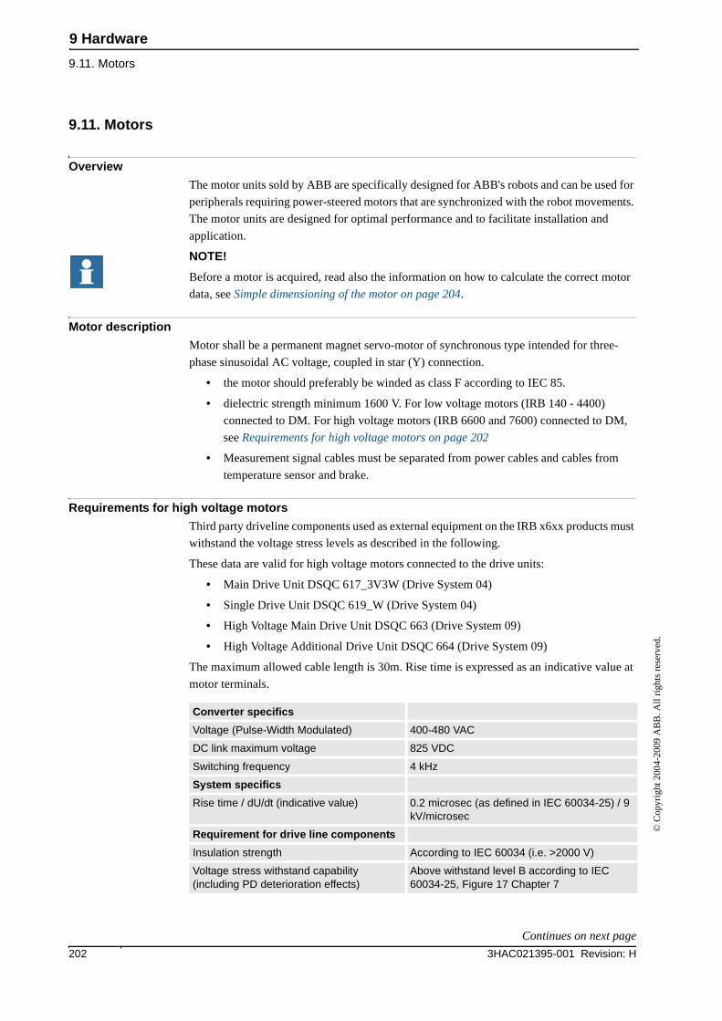
9 Hardware
9.11. Motors
3HAC021395-001 Revision: H202
© C
opyr
ight
200
4-20
09 A
BB
. All
righ
ts r
eser
ved.
9.11. Motors
Overview
The motor units sold by ABB are specifically designed for ABB's robots and can be used for
peripherals requiring power-steered motors that are synchronized with the robot movements.
The motor units are designed for optimal performance and to facilitate installation and
application.
NOTE!
Before a motor is acquired, read also the information on how to calculate the correct motor
data, see Simple dimensioning of the motor on page 204.
Motor description
Motor shall be a permanent magnet servo-motor of synchronous type intended for three-
phase sinusoidal AC voltage, coupled in star (Y) connection.
• the motor should preferably be winded as class F according to IEC 85.
• dielectric strength minimum 1600 V. For low voltage motors (IRB 140 - 4400)
connected to DM. For high voltage motors (IRB 6600 and 7600) connected to DM,
see Requirements for high voltage motors on page 202
• Measurement signal cables must be separated from power cables and cables from
temperature sensor and brake.
Requirements for high voltage motors
Third party driveline components used as external equipment on the IRB x6xx products must
withstand the voltage stress levels as described in the following.
These data are valid for high voltage motors connected to the drive units:
• Main Drive Unit DSQC 617_3V3W (Drive System 04)
• Single Drive Unit DSQC 619_W (Drive System 04)
• High Voltage Main Drive Unit DSQC 663 (Drive System 09)
• High Voltage Additional Drive Unit DSQC 664 (Drive System 09)
The maximum allowed cable length is 30m. Rise time is expressed as an indicative value at
motor terminals.
Converter specifics
Voltage (Pulse-Width Modulated) 400-480 VAC
DC link maximum voltage 825 VDC
Switching frequency 4 kHz
System specifics
Rise time / dU/dt (indicative value) 0.2 microsec (as defined in IEC 60034-25) / 9 kV/microsec
Requirement for drive line components
Insulation strength According to IEC 60034 (i.e. >2000 V)
Voltage stress withstand capability (including PD deterioration effects)
Above withstand level B according to IEC 60034-25, Figure 17 Chapter 7
Continues on next page
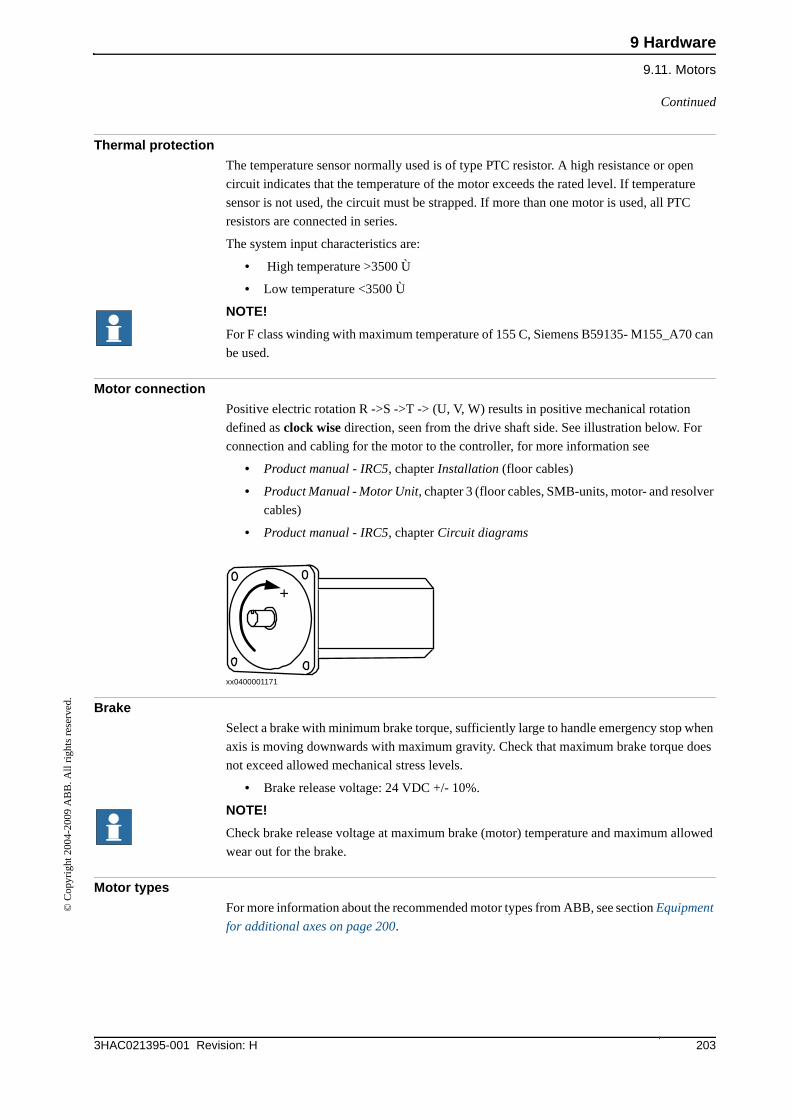
9 Hardware
9.11. Motors
2033HAC021395-001 Revision: H
© C
opyr
ight
200
4-20
09 A
BB
. All
righ
ts r
eser
ved.
Thermal protection
The temperature sensor normally used is of type PTC resistor. A high resistance or open
circuit indicates that the temperature of the motor exceeds the rated level. If temperature
sensor is not used, the circuit must be strapped. If more than one motor is used, all PTC
resistors are connected in series.
The system input characteristics are:
• High temperature >3500 Ù
• Low temperature <3500 Ù
NOTE!
For F class winding with maximum temperature of 155 C, Siemens B59135- M155_A70 can
be used.
Motor connection
Positive electric rotation R ->S ->T -> (U, V, W) results in positive mechanical rotation
defined as clock wise direction, seen from the drive shaft side. See illustration below. For
connection and cabling for the motor to the controller, for more information see
• Product manual - IRC5, chapter Installation (floor cables)
• Product Manual - Motor Unit, chapter 3 (floor cables, SMB-units, motor- and resolver
cables)
• Product manual - IRC5, chapter Circuit diagrams
xx0400001171
Brake
Select a brake with minimum brake torque, sufficiently large to handle emergency stop when
axis is moving downwards with maximum gravity. Check that maximum brake torque does
not exceed allowed mechanical stress levels.
• Brake release voltage: 24 VDC +/- 10%.
NOTE!
Check brake release voltage at maximum brake (motor) temperature and maximum allowed
wear out for the brake.
Motor types
For more information about the recommended motor types from ABB, see section Equipment
for additional axes on page 200.
+
Continued
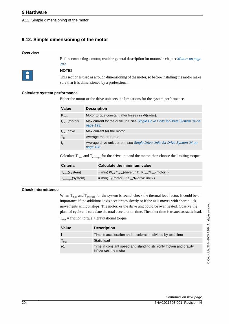
9 Hardware
9.12. Simple dimensioning of the motor
3HAC021395-001 Revision: H204
© C
opyr
ight
200
4-20
09 A
BB
. All
righ
ts r
eser
ved.
9.12. Simple dimensioning of the motor
Overview
Before connecting a motor, read the general description for motors in chapter Motors on page
202
NOTE!
This section is used as a rough dimensioning of the motor, so before installing the motor make
sure that it is dimensioned by a professional.
Calculate system performance
Either the motor or the drive unit sets the limitations for the system performance.
Calculate Tmax and Taverage for the drive unit and the motor, then choose the limiting torque.
Check intermittence
When Tmax and Taverage for the system is found, check the thermal load factor. It could be of
importance if the additional axis accelerates slowly or if the axis moves with short quick
movements without stops. The motor, or the drive unit could be over heated. Observe the
planned cycle and calculate the total acceleration time. The other time is treated as static load.
Tstat = friction torque + gravitational torque
Value Description
Ktmin Motor torque constant after losses in V/(rad/s).
Imax (motor) Max current for the drive unit, see Single Drive Units for Drive System 04 on page 193.
Imax drive Max current for the motor
T0 Average motor torque
I0 Average drive unit current, see Single Drive Units for Drive System 04 on page 193.
Criteria Calculate the minimum value
Tmax(system) = min( Ktmin*Imax(drive unit), Ktmin*Imax(motor) )
Taverage(system) = min( T0(motor), Ktmin*I0(drive unit) )
Value Description
i Time in acceleration and deceleration divided by total time
Tstat Static load
i-1 Time in constant speed and standing still (only friction and gravity influences the motor
Continues on next page
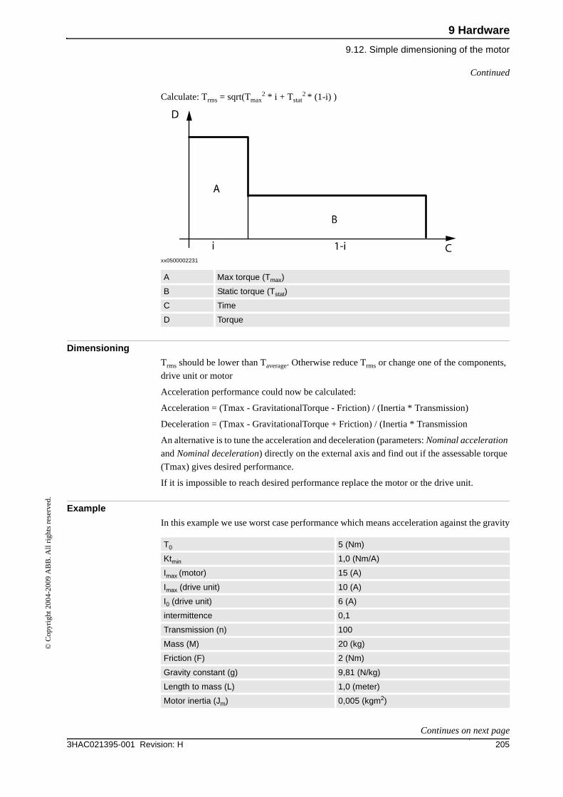
9 Hardware
9.12. Simple dimensioning of the motor
2053HAC021395-001 Revision: H
© C
opyr
ight
200
4-20
09 A
BB
. All
righ
ts r
eser
ved.
Calculate: Trms = sqrt(Tmax2 * i + Tstat
2 * (1-i) )
xx0500002231
Dimensioning
Trms should be lower than Taverage. Otherwise reduce Trms or change one of the components,
drive unit or motor
Acceleration performance could now be calculated:
Acceleration = (Tmax - GravitationalTorque - Friction) / (Inertia * Transmission)
Deceleration = (Tmax - GravitationalTorque + Friction) / (Inertia * Transmission
An alternative is to tune the acceleration and deceleration (parameters: Nominal acceleration
and Nominal deceleration) directly on the external axis and find out if the assessable torque
(Tmax) gives desired performance.
If it is impossible to reach desired performance replace the motor or the drive unit.
Example
In this example we use worst case performance which means acceleration against the gravity
A Max torque (Tmax)
B Static torque (Tstat)
C Time
D Torque
T0 5 (Nm)
Ktmin 1,0 (Nm/A)
Imax (motor) 15 (A)
Imax (drive unit) 10 (A)
I0 (drive unit) 6 (A)
intermittence 0,1
Transmission (n) 100
Mass (M) 20 (kg)
Friction (F) 2 (Nm)
Gravity constant (g) 9,81 (N/kg)
Length to mass (L) 1,0 (meter)
Motor inertia (Jm) 0,005 (kgm2)
Continued
Continues on next page
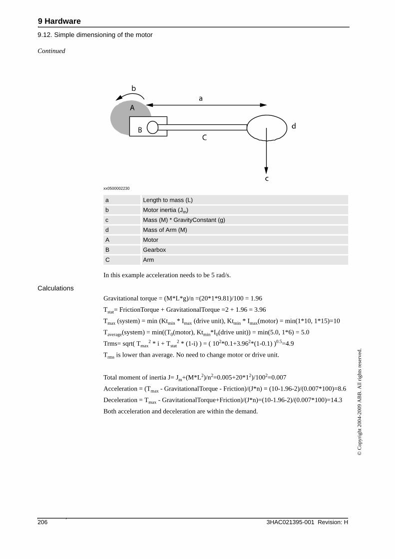
9 Hardware
9.12. Simple dimensioning of the motor
3HAC021395-001 Revision: H206
© C
opyr
ight
200
4-20
09 A
BB
. All
righ
ts r
eser
ved.
xx0500002230
In this example acceleration needs to be 5 rad/s.
Calculations
Gravitational torque = (M*L*g)/n =(20*1*9.81)/100 = 1.96
Tstat= FrictionTorque + GravitationalTorque =2 + 1.96 = 3.96
Tmax (system) = min (Ktmin * Imax (drive unit), Ktmin * Imax(motor) = min(1*10, 1*15)=10
Taverage(system) = min((T0(motor), Ktmin*I0(drive unit)) = min(5.0, 1*6) = 5.0
Trms= sqrt( Tmax2 * i + Tstat
2 * (1-i) ) = ( 102*0.1+3.962*(1-0.1) )0.5=4.9
Trms is lower than average. No need to change motor or drive unit.
Total moment of inertia J= Jm+(M*L2)/n2=0.005+20*12)/1002=0.007
Acceleration = (Tmax - GravitationalTorque - Friction)/(J*n) = (10-1.96-2)/(0.007*100)=8.6
Deceleration = Tmax - GravitationalTorque+Friction)/(J*n)=(10-1.96-2)/(0.007*100)=14.3
Both acceleration and deceleration are within the demand.
a Length to mass (L)
b Motor inertia (Jm)
c Mass (M) * GravityConstant (g)
d Mass of Arm (M)
A Motor
B Gearbox
C Arm
Continued
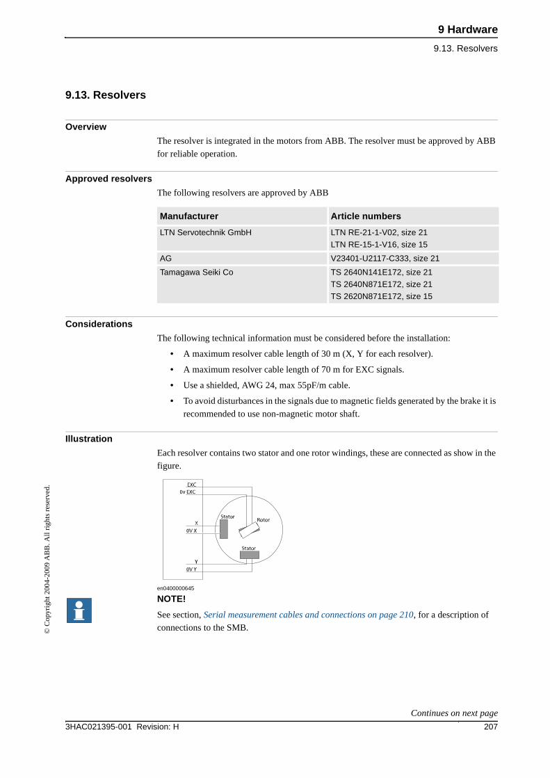
9 Hardware
9.13. Resolvers
2073HAC021395-001 Revision: H
© C
opyr
ight
200
4-20
09 A
BB
. All
righ
ts r
eser
ved.
9.13. Resolvers
Overview
The resolver is integrated in the motors from ABB. The resolver must be approved by ABB
for reliable operation.
Approved resolvers
The following resolvers are approved by ABB
Considerations
The following technical information must be considered before the installation:
• A maximum resolver cable length of 30 m (X, Y for each resolver).
• A maximum resolver cable length of 70 m for EXC signals.
• Use a shielded, AWG 24, max 55pF/m cable.
• To avoid disturbances in the signals due to magnetic fields generated by the brake it is
recommended to use non-magnetic motor shaft.
Illustration
Each resolver contains two stator and one rotor windings, these are connected as show in the
figure.
en0400000645
NOTE!
See section, Serial measurement cables and connections on page 210, for a description of
connections to the SMB.
Manufacturer Article numbers
LTN Servotechnik GmbH LTN RE-21-1-V02, size 21
LTN RE-15-1-V16, size 15
AG V23401-U2117-C333, size 21
Tamagawa Seiki Co TS 2640N141E172, size 21
TS 2640N871E172, size 21
TS 2620N871E172, size 15
Continues on next page
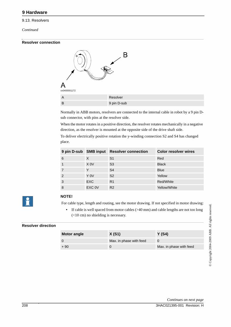
9 Hardware
9.13. Resolvers
3HAC021395-001 Revision: H208
© C
opyr
ight
200
4-20
09 A
BB
. All
righ
ts r
eser
ved.
Resolver connection
xx0400001172
Normally in ABB motors, resolvers are connected to the internal cable in robot by a 9 pin D-
sub connector, with pins at the resolver side.
When the motor rotates in a positive direction, the resolver rotates mechanically in a negative
direction, as the resolver is mounted at the opposite side of the drive shaft side.
To deliver electrically positive rotation the y-winding connection S2 and S4 has changed
place.
NOTE!
For cable type, length and routing, see the motor drawing. If not specified in motor drawing:
• If cable is well spaced from motor cables (>40 mm) and cable lengths are not too long
(<10 cm) no shielding is necessary.
Resolver direction
A Resolver
B 9 pin D-sub
9 pin D-sub SMB input Resolver connection Color resolver wires
6 X S1 Red
1 X 0V S3 Black
7 Y S4 Blue
2 Y 0V S2 Yellow
3 EXC R1 Red/White
8 EXC 0V R2 Yellow/White
Motor angle X (S1) Y (S4)
0 Max. in phase with feed 0
+ 90 0 Max. in phase with feed
Continued
Continues on next page
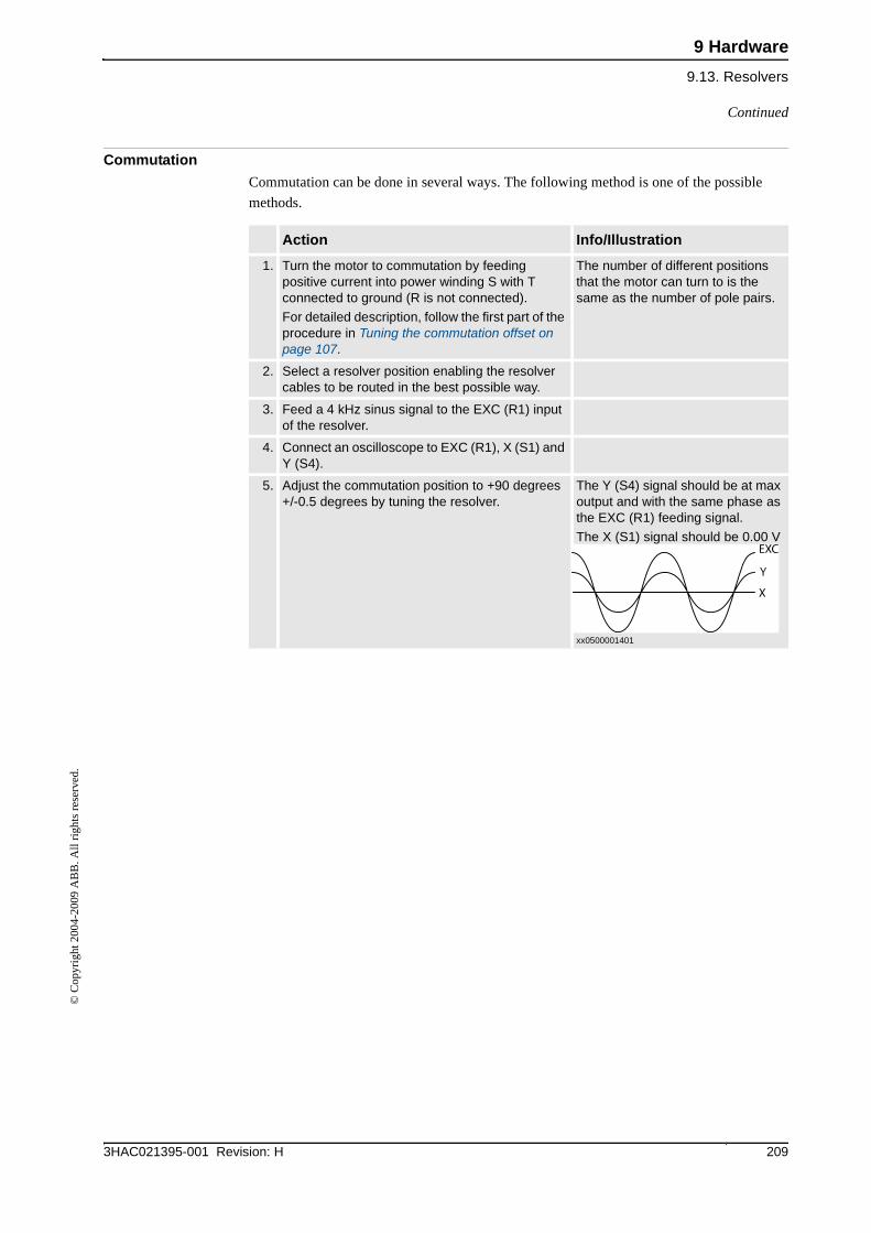
9 Hardware
9.13. Resolvers
2093HAC021395-001 Revision: H
© C
opyr
ight
200
4-20
09 A
BB
. All
righ
ts r
eser
ved.
Commutation
Commutation can be done in several ways. The following method is one of the possible
methods.
Action Info/Illustration
1. Turn the motor to commutation by feeding positive current into power winding S with T connected to ground (R is not connected).
For detailed description, follow the first part of the procedure in Tuning the commutation offset on page 107.
The number of different positions that the motor can turn to is the same as the number of pole pairs.
2. Select a resolver position enabling the resolver cables to be routed in the best possible way.
3. Feed a 4 kHz sinus signal to the EXC (R1) input of the resolver.
4. Connect an oscilloscope to EXC (R1), X (S1) and Y (S4).
5. Adjust the commutation position to +90 degrees +/-0.5 degrees by tuning the resolver.
The Y (S4) signal should be at max output and with the same phase as the EXC (R1) feeding signal.
The X (S1) signal should be 0.00 V
xx0500001401
Continued
9 Hardware
9.14. Serial measurement cables and connections
3HAC021395-001 Revision: H210
© C
opyr
ight
200
4-20
09 A
BB
. All
righ
ts r
eser
ved.
9.14. Serial measurement cables and connections
Overview
This section details the cables and connection between the resolver and the serial
measurement board.
Signal Classes
The cabling must comply with a valid signal class "measurement signals" see Product manual
for controller IRC5, section Signal Classes. The enclosure for external serial measurement
board/boards must comply with enclosure class IP54, in accordance with IEC 144 and IEC
529.
NOTE!
It is very important that the noise level on the measurement signals from the additional axes
is kept as low as possible, to prevent bad performance, (keep motor and resolver cables apart). Correct shielding and ground connections of cables, measurement boards and
resolvers is essential.
Considerations
The X, Y, 0V X and 0V Y:
• Signals are used to connect resolvers to a serial measurement board.
The EXC and 0V EXC:
• are used for common supply for all resolvers, parallel connected.
Resolver:
• 1 - 3, should always be connected to EXC 1.
• 4 - 7, should always be connected to EXC 2.
NOTE!
Maximum allowed lenght on the serial measurement cable is 50 meters.
Continues on next page
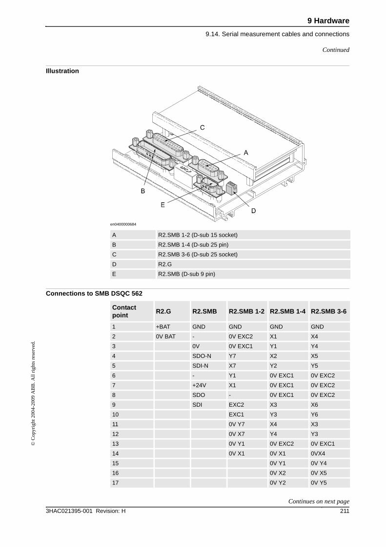
9 Hardware
9.14. Serial measurement cables and connections
2113HAC021395-001 Revision: H
© C
opyr
ight
200
4-20
09 A
BB
. All
righ
ts r
eser
ved.
Illustration
en0400000684
Connections to SMB DSQC 562
A R2.SMB 1-2 (D-sub 15 socket)
B R2.SMB 1-4 (D-sub 25 pin)
C R2.SMB 3-6 (D-sub 25 socket)
D R2.G
E R2.SMB (D-sub 9 pin)
Contact point
R2.G R2.SMB R2.SMB 1-2 R2.SMB 1-4 R2.SMB 3-6
1 +BAT GND GND GND GND
2 0V BAT - 0V EXC2 X1 X4
3 0V 0V EXC1 Y1 Y4
4 SDO-N Y7 X2 X5
5 SDI-N X7 Y2 Y5
6 - Y1 0V EXC1 0V EXC2
7 +24V X1 0V EXC1 0V EXC2
8 SDO - 0V EXC1 0V EXC2
9 SDI EXC2 X3 X6
10 EXC1 Y3 Y6
11 0V Y7 X4 X3
12 0V X7 Y4 Y3
13 0V Y1 0V EXC2 0V EXC1
14 0V X1 0V X1 0VX4
15 0V Y1 0V Y4
16 0V X2 0V X5
17 0V Y2 0V Y5
Continued
Continues on next page
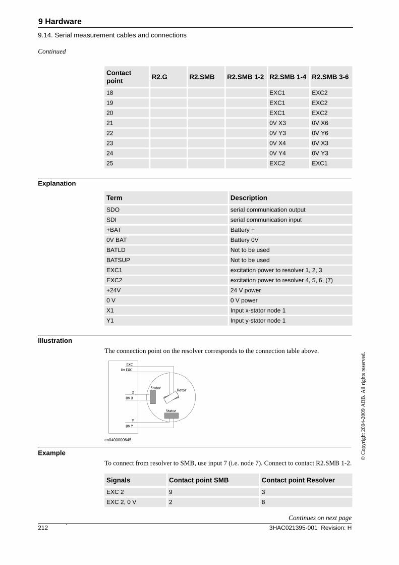
9 Hardware
9.14. Serial measurement cables and connections
3HAC021395-001 Revision: H212
© C
opyr
ight
200
4-20
09 A
BB
. All
righ
ts r
eser
ved.
Explanation
Illustration
The connection point on the resolver corresponds to the connection table above.
en0400000645
Example
To connect from resolver to SMB, use input 7 (i.e. node 7). Connect to contact R2.SMB 1-2.
18 EXC1 EXC2
19 EXC1 EXC2
20 EXC1 EXC2
21 0V X3 0V X6
22 0V Y3 0V Y6
23 0V X4 0V X3
24 0V Y4 0V Y3
25 EXC2 EXC1
Contact point
R2.G R2.SMB R2.SMB 1-2 R2.SMB 1-4 R2.SMB 3-6
Term Description
SDO serial communication output
SDI serial communication input
+BAT Battery +
0V BAT Battery 0V
BATLD Not to be used
BATSUP Not to be used
EXC1 excitation power to resolver 1, 2, 3
EXC2 excitation power to resolver 4, 5, 6, (7)
+24V 24 V power
0 V 0 V power
X1 Input x-stator node 1
Y1 Input y-stator node 1
Signals Contact point SMB Contact point Resolver
EXC 2 9 3
EXC 2, 0 V 2 8
Continued
Continues on next page
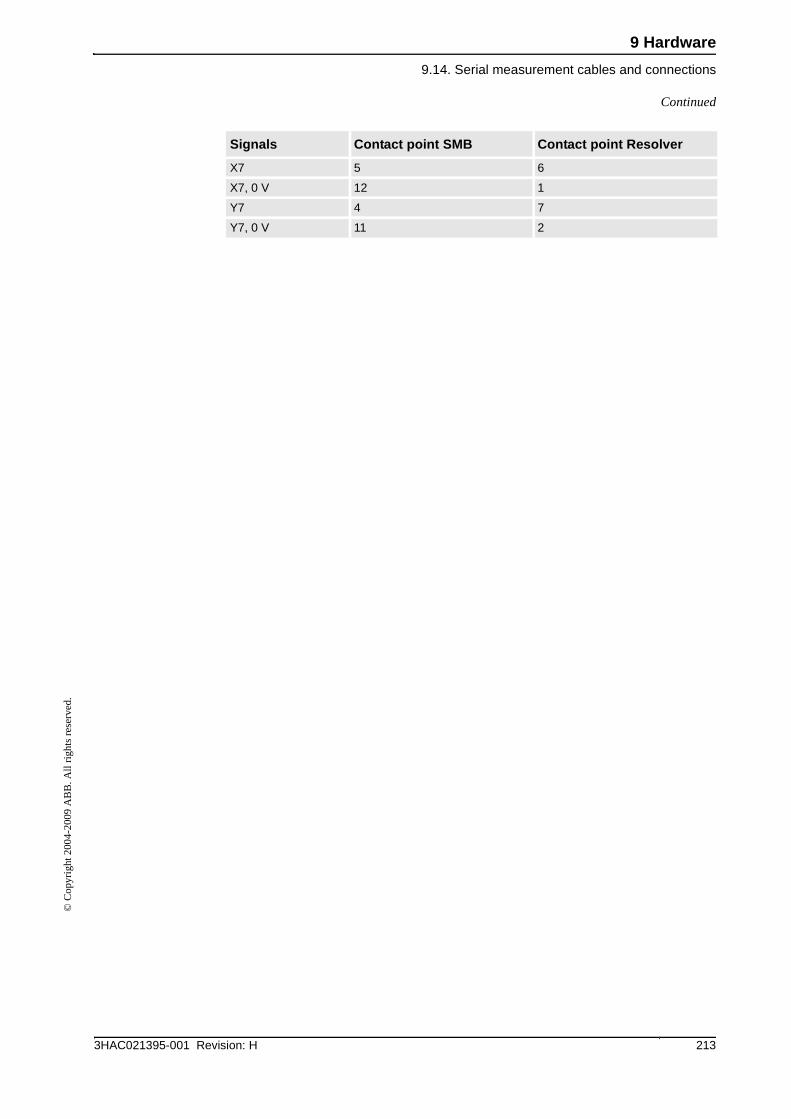
9 Hardware
9.14. Serial measurement cables and connections
2133HAC021395-001 Revision: H
© C
opyr
ight
200
4-20
09 A
BB
. All
righ
ts r
eser
ved.
X7 5 6
X7, 0 V 12 1
Y7 4 7
Y7, 0 V 11 2
Signals Contact point SMB Contact point Resolver
Continued
9 Hardware
9.14. Serial measurement cables and connections
3HAC021395-001 Revision: H214
© C
opyr
ight
200
4-20
09 A
BB
. All
righ
ts r
eser
ved.
Index
2153HAC021395-001 Revision: H
© C
opyr
ight
200
4-20
09 A
BB
. All
righ
ts r
eser
ved.
AAdditional axes 14
Bbase frame 96Base frame moved by 94brake release box 200brakes 201
Ccables 200capacitor 181Configuration of the drive system 181, 189coordinated axes 93coordination procedure 94, 98
Ddrive unit 189Drive unit Node 187drive units 181, 189
Ffilters 181, 189
Ggear ratio 15
Iindependent programming 14
Mmain drive unit 189mechanical unit 93motors 201MultiMove system 14multiple axes positioner 102
Nnon-MultiMove system 14
Ppositioner 98
Rrectifiers 181, 189resolvers 201revolution counter 15robot 14
Ssafety 11serial measurement box 200servo drive units 181Stand alone controller 14
Ttrack motion 94transmission gear ratio 15two axes positioner 102
Uuser coordinate system 98
user frame 99, 102

Index
216 3HAC021395-001 Revision: H
© C
opyr
ight
200
4-20
09 A
BB
. All
righ
ts r
eser
ved.


ABB ABRobotics ProductsS-721 68 VÄSTERÅSSWEDENTelephone: +46 (0) 21 344000Telefax: +46 (0) 21 132592
3HA
C02
1395
-001
, Rev
isio
n H
, en


![Robotware 6 External Presentation.ppt - ABB Ltd · Microsoft PowerPoint - Robotware 6 External Presentation.ppt [Compatibility Mode] Author: SENISAL Created Date: 12/16/2014 11:35:06](https://img.pdfslide.us/doc/110x75/5acb47877f8b9aa3298e4c55/robotware-6-external-abb-ltd-powerpoint-robotware-6-external-compatibility.jpg)