IMF Country Report No. 16/347 ARGENTINA Country Report No. 16/347 ARGENTINA SELECTED ISSUES This Selected Issues paper on Argentina was prepared by a staff team of the International

© 2016 International Monetary Fund

IMF Country Report No. 16/347

ARGENTINA SELECTED ISSUES

This Selected Issues paper on Argentina was prepared by a staff team of the International

Monetary Fund. It is based on the information available at the time it was completed on

October 26, 2016.

Copies of this report are available to the public from

International Monetary Fund Publication Services

PO Box 92780 Washington, D.C. 20090

Telephone: (202) 623-7430 Fax: (202) 623-7201

E-mail: [email protected] Web: http://www.imf.org

Price: $18.00 per printed copy

International Monetary Fund

Washington, D.C.

November 2016

mailto:[email protected]

http://www.imf.org/

ARGENTINA SELECTED ISSUES

Approved By Nigel Chalk

Prepared by Jorge Iván Canales-Kriljenko, Paolo Dudine, Luis

Jácome, Lusine Lusinyan, Mariano Ortiz Villafañe, Alex

Pienkowski, José Luis Saboin, and Diva Singh

HOW LARGE IS ARGENTINA'S CAPITAL ACCUMULATION GAP AND HOW CAN

IT BE REDUCED? LESSONS FROM PAST INVESTMENT SURGES _________________ 6

A. Introduction _____________________________________________________________________ 6

B. Assessing Argentina's "Capital Accumulation Gap" ______________________________ 8

C. What Drives Investment Surges? An Event Analysis _____________________________ 14

References ________________________________________________________________________ 22

FIGURES

1. Nominal Fixed Capital Formation: 1981–2015 ____________________________________ 7

2. Private Nominal Fixed Capital Formation: 1981–2015 ____________________________ 7

3. Public Nominal Fixed Capital Formation: 1981–2015 _____________________________ 7

4. GDP Per Capita: 1981–2015 ______________________________________________________ 7

5. Factors of Production, Alternative Data Sources: 1981–2015 _____________________ 8

6. Capital-to-Output Ratio: 1980–2014 _____________________________________________ 9

7. Capital-to-Labor Ratio: 1980–2015 _______________________________________________ 9

8. Growth in Capital-Labor Ratio Required to Catch Up with Peer Median ________ 10

9. Investment Required to Reach Median Capital-to-Labor Intensity ______________ 11

10. Capital/Output and Investment Rate in 2014, Relative to Estimated

Long-Run Levels_______________________________________________________________ 11

11. Sensitivity of Steady-State Investment Rates to Alternative Parameter

Specification __________________________________________________________________ 12

12. Infrastructure Indicators: Argentina's Percentile in Distribution of Peer Advanced

and Emerging Markets ________________________________________________________ 13

13. Event Analysis Charts __________________________________________________________ 17

14. Frequency of Investment Surge Episodes ______________________________________ 17

CONTENTS

October 26, 2016

ARGENTINA

2 INTERNATIONAL MONETARY FUND

TABLES

1. Investment Surge Episodes: 1981–2015 _________________________________________ 15

2. Hodges-Lehman Median Differences on Investment Surge Episodes ___________ 16

3. Direction of Variation of Key Variables During Episodes ________________________ 18

4. Bilateral Panel Logit Regressions ________________________________________________ 20

5. Multilateral Panel Logit Regressions ____________________________________________ 21

ANNEXES

I. Panel Investment and Growth __________________________________________________ 25

II. Panel Production Function _____________________________________________________ 28

III. Panel Charts for Selected Investment Surge Episodes __________________________ 31

ARGENTINA'S FISCAL ADJUSTMENT: HOW CAN IT BE DONE? ________________ 37

A. Introduction ____________________________________________________________________ 37

B. Primary Expenditure ____________________________________________________________ 39

C. Tax Revenues ___________________________________________________________________ 47

D. Assessing the Economic Impact of Fiscal Consolidation ________________________ 50

References ________________________________________________________________________ 55

BOXES

1. Decomposing the Price and Volume Effects Driving Public Expenditure Growth 43

2. Measuring the Impact of Subsidy Reform on the Most Vulnerable______________ 45

FIGURE

1. Partially Credible Policies, With vs. Without Monetary Reaction_________________ 53

ANNEX

I. Model Description and Fiscal Policy Analysis ___________________________________ 57

ARGENTINA’S PENSION AND SOCIAL SECURITY SYSTEM: A SUSTAINABILITY

ANALYSIS ________________________________________________________________________ 60

A. Introduction ____________________________________________________________________ 60

B. The System _____________________________________________________________________ 61

C. Reform Proposals _______________________________________________________________ 67

ARGENTINA

INTERNATIONAL MONETARY FUND 3

References ________________________________________________________________________ 69

BOXES

1. Argentina’s Current Pension System ____________________________________________ 62

2. The Indexation Formula (La Fórmula de Movilidad) _____________________________ 63

3. History of Argentina’s Social Security System ___________________________________ 64

FIGURE

1. Argentina: Social Security Coverage, Benefits, and Spending ___________________ 66

ANNEX

I. The Model _______________________________________________________________________ 70

DISINFLATION UNDER INFLATION TARGETING: A SMALL MACRO MODEL FOR

ARGENTINA ______________________________________________________________________ 72

A. The Model ______________________________________________________________________ 73

B. Data and Estimation ____________________________________________________________ 74

C. Implications for Monetary Policy________________________________________________ 80

References ________________________________________________________________________ 85

FIGURES

1. Impulse Response to an Interest Rate Shock ____________________________________ 79

2. Impulse Response to a Domestic Demand Shock _______________________________ 79

3. Argentine Disinflation Path with Optimal Policy Rule ___________________________ 80

4. Sensitivity of Potential Output Cost of Disinflation to Different Degrees of

Inflation Inertia _________________________________________________________________ 82

5. Sensitivity of Potential Output Cost of Disinflation to Weights in Loss Function 83

6. Simulations of Disinflation with Real Exchange Rate Volatility in Loss ___________ 84

TABLE

1. Parameter Estimates ____________________________________________________________ 76

ANNEX

I. The Model _______________________________________________________________________ 89

ARGENTINA


ENHANCING THE EFFECTIVENESS OF INFLATION TARGETING IN

ARGENTINA ______________________________________________________________________ 92

A. Introduction ____________________________________________________________________ 92

B. The Road to Inflation Targeting _________________________________________________ 94

C. Strengthening the Institutional Foundations of Monetary Policy _______________ 99

D. Further Refinements on the Monetary Policy Framework ______________________ 102

References _______________________________________________________________________ 107

BOXES

1. A Snapshot of Inflation and Stabilization Plans in Argentina in the

Last 50 Years ____________________________________________________________________ 93

2. Inflation Inertia in Argentina and Other Selected Latin American Countries _____ 98

3. Key Principles to Rule Central Bank Credit to the Government _________________ 102

FIGURES

1. Moderate Inflation in Argentina ________________________________________________ 94

2. Inflation Expectations ___________________________________________________________ 94

3. Inflation at Inception of Inflation Targeting _____________________________________ 95

4. Moderate Inflation Episodes and Convergence to Low Inflation ________________ 96

5. Primary Balance at Inflation Targeting Inception ________________________________ 97

6. Independence of the BCRA ____________________________________________________ 100

7. Central Bank Independence ____________________________________________________ 100

TABLE

1. Monetary Policy Decision-Making in Selected Inflation Targeting Countries ___ 104

APPENDICES

I. Monetary Policy ________________________________________________________________ 109

II. Turkey’s Transition to Inflation Targeting ______________________________________ 110

ARGENTINA'S EXPORTS AND COMPETITIVENESS: A SECTORAL VIEW ON

TRENDS AND PROSPECTS _____________________________________________________ 111

A. Introduction ___________________________________________________________________ 111

B. Argentina’s Exports Over the Last Decade: A Few Trends ______________________ 113

C. Price Competitiveness: A Product-Level Analysis ______________________________ 114

D. Non-Price Competitiveness: A Few Considerations ____________________________ 118

ARGENTINA


References _______________________________________________________________________ 121

FIGURES

1. Price Competitiveness _________________________________________________________ 112

2. Argentina’s Exports: Changes in Composition and Market Share ______________ 113

APPENDICES

I. Data Sources and Description _________________________________________________ 122

II. Empirical Results and Robustness Analysis ____________________________________ 124

MEDIUM-TERM PROSPECTS FOR ARGE NTINA'S EXTERNAL

BALANCE SHEET _______________________________________________________________ 128

A. Introduction ___________________________________________________________________ 128

B. The External Balance Sheet Today _____________________________________________ 129

C. Estimating the Medium-Term Position _________________________________________ 131

D. Conclusion ____________________________________________________________________ 137

FIGURES

1. IIP by Asset and Liability Type, 2002–15 ________________________________________ 128

2. Capital Account Oppeness Index, ______________________________________________ 128

3. IIP Relative to Regional Peers, 2014 ____________________________________________ 130

4. Sectoral Breakdown of External Debt, 2015Q2 _________________________________ 130

5. Currency Composition of External Assets and Liabilities, 2012 _________________ 131

6. Maturity Structure of External Debt, 2015Q2 ___________________________________ 131

7. External Assets and Liabilities __________________________________________________ 134

8. Net IIP _________________________________________________________________________ 134

9. Selected Indicators from External Balance Sheet Expansion Episodes __________ 136

TABLE

1. Initial Conditions for Event Analysis Episodes __________________________________ 135

APPENDIX _______________________________________________________________________ 139

ARGENTINA


HOW LARGE IS ARGENTINA’S CAPITAL ACCUMULATION GAP AND HOW CAN IT BE REDUCED? LESSONS FROM PAST INVESTMENT SURGES1

A. Introduction

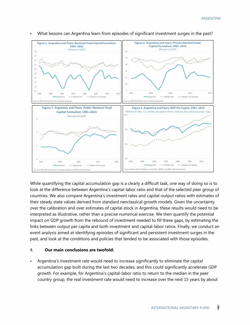
1. Over the last three and a half decades, Argentina’s investment rate has been among

the lowest among peer advanced and emerging market countries. Investment rates (defined in

this paper as gross fixed capital formation in percent of GDP) fell in the 1980s from already relatively

low levels and recovered strongly in the 1990s. After rebounding rapidly from the historical lows

experienced during the 2001 economic crisis, the investment rate fell again over the last decade,

reflecting the deterioration of the macroeconomic environment and increasing government

interventionist policies (Figure 1). As of 2015, Argentina’s investment rate was well below the average

of Latin American countries and that of a peer group of advanced and emerging market countries,

with a larger gap in private investment (Figures 2 and 3).2 The low investment rates may have

contributed to the relative decline in Argentina’s GDP per capita over the same period (Figure 4).

2. Raising investment prospects would be essential to boost economic activity. The

administration that took office in December 2015 has emphasized the importance of generating an

investor friendly environment that allows Argentina to recover some of the growth opportunities lost

over the last few decades. With this in mind, the administration promptly removed exchange and

capital controls, resolved its outstanding external debt disputes to regain access to international

capital markets, and started the process of subsidy reform. In addition to structural reforms that

foster investment (IMF, forthcoming), stabilizing the macroeconomic environment would be an

important trigger for an investment rebound.

3. In this paper we address the following questions:

How large is the “capital accumulation gap” from Argentina’s low investment rate of the last two

decades? What would be the increase in investment needed to close that gap, and how sizeable

would be the boost on output?

1 Prepared by Jorge Iván Canales-Kriljenko.

2 To bring into the discussion the international experience, we compare developments in Argentina with those in a

group of 32 other peer countries, selected to include all G-20 countries, 20 large emerging markets, all BRICS, five

other large Latin American countries and peer historical development partners like Spain. All key trading partners are

included. The peer group attempts to inform the evolution of developments in Argentina from countries that either

face similar issues or that have higher income levels to which Argentina may aspire. The peer group includes, among

advanced economies, Australia, Canada, Czech Republic, France, Germany, Israel, Italy, Japan, Korea, New Zealand,

Spain, United Kingdom, and the United States, and among emerging markets, Argentina, Brazil, Chile, China,

Colombia, Hungary, India, Indonesia, Malaysia, Mexico, Peru, Philippines, Poland, Russia, Saudi Arabia, South Africa,

Thailand, Turkey, Ukraine, and Vietnam.

ARGENTINA


What lessons can Argentina learn from episodes of significant investment surges in the past?

While quantifying the capital accumulation gap is a clearly a difficult task, one way of doing so is to

look at the difference between Argentina’s capital-labor ratio and that of the selected peer group of

countries. We also compare Argentina’s investment rates and capital-output ratios with estimates of

their steady state values derived from standard neoclassical growth models. Given the uncertainty

over the calibration and over estimates of capital stock in Argentina, these results would need to be

interpreted as illustrative, rather than a precise numerical exercise. We then quantify the potential

impact on GDP growth from the rebound of investment needed to fill these gaps, by estimating the

links between output per capita and both investment and capital-labor ratios. Finally, we conduct an

event analysis aimed at identifying episodes of significant and persistent investment surges in the

past, and look at the conditions and policies that tended to be associated with those episodes.

4. Our main conclusions are twofold:

Argentina’s investment rate would need to increase significantly to eliminate the capital

accumulation gap built during the last two decades, and this could significantly accelerate GDP

growth. For example, for Argentina’s capital-labor ratio to return to the median in the peer

country group, the real investment rate would need to increase over the next 15 years by about

8.5

9.0

9.5

10.0

1980 1985 1990 1995 2000 2005 2010

Argentina Median EM Median full sample

Figure 4. Argentina and Peers: GDP Per Capita: 1981–2015

Millions of 2011 U.S. dollars per person (from constant 2011 national prices, logs)

Sources: Penn World Tables (version 9.0), INDEC, and IMF staff calculations.

8

10

12

14

16

18

20

1995 2000 2005 2010 2015

Argentina Median EM Median Full Sample

Figure 2. Argentina and Peers: Private Nominal Fixed

Capital Formation: 1981–2015

(Percent of GDP)

Sources: IMF World Economic Outlook database.

10

12

14

16

18

20

22

24

26

28

1980 1985 1990 1995 2000 2005 2010 2015


Figure 1. Argentina and Peers: Nominal Fixed Capital Formation:

1981–2015

(Percent of GDP)

Sources: IMF World Economic Outlook database.

(Percent of GDP)

Figure 3. Argentina and Peers: Public Nominal Fixed

Capital Formation: 1981–2015

0

2

4

6

1995 2000 2005 2010 2015


Figure 3. Argentina and Peers: Public Nominal Fixed Capital Formation:

1981-2015

(Percent of GDP)

Sources: IMF World Economic Outlook database and IMF staff estimates.

ARGENTINA


10 percentage points of GDP, with a potential positive impact on GDP growth by between about

1 and 3 percent per annum over the same period. The existence of a capital accumulation gap

suggests that Argentina could well be bound to experience a significant investment surge.

The event analysis shows that investment surges generally build over many years, and tend to

coincide with an increase in national saving rate supported by fiscal consolidation. This suggests

that a prudent fiscal policy, able to reallocate spending to increase public investment while

gradually reducing the fiscal deficit, would facilitate the needed investment rebound.

B. Assessing Argentina’s “Capital Accumulation Gap”

Figure 5. Argentina: Factors of Production, Alternative Data Sources: 1981–2015

(Percent of GDP)

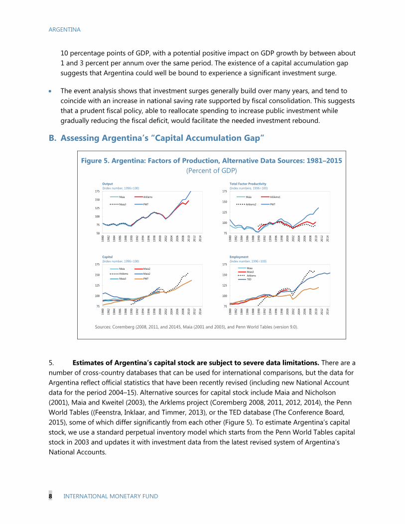
5. Estimates of Argentina’s capital stock are subject to severe data limitations. There are a

number of cross-country databases that can be used for international comparisons, but the data for

Argentina reflect official statistics that have been recently revised (including new National Account

data for the period 2004–15). Alternative sources for capital stock include Maia and Nicholson

(2001), Maia and Kweitel (2003), the Arklems project (Coremberg 2008, 2011, 2012, 2014), the Penn

World Tables ((Feenstra, Inklaar, and Timmer, 2013), or the TED database (The Conference Board,

2015), some of which differ significantly from each other (Figure 5). To estimate Argentina’s capital

stock, we use a standard perpetual inventory model which starts from the Penn World Tables capital

stock in 2003 and updates it with investment data from the latest revised system of Argentina’s

National Accounts.

50

75

100

125

150

175

1980

1982

1984

1986

1988

1990

1992

1994

1996

1998

2000

2002

2004

2006

2008

2010

2012

2014

Maia Arklems

Maia3 PWT

Output

(Index number, 1996=100)

75

100

125

150

175

1980

1982

1984

1986

1988

1990

1992

1994

1996

1998

2000

2002

2004

2006

2008

2010

2012

2014

Maia Arklems1

Arklems2 PWT

Total Factor Productivity

(Index numbers, 1996=100)

75

100

125

150

175

1980

1982

1984

1986

1988

1990

1992

1994

1996

1998

2000

2002

2004

2006

2008

2010

2012

2014

Maia Maia2

Arklems Maia2

Maia3 PWT

Capital


75

100

125

150

175

1980

1982

1984

1986

1988

1990

1992

1994

1996

1998

2000

2002

2004

2006

2008

2010

2012

2014

Maia

Maia3

Arklems

TED

Employment


Figure 5. Argentina: Factors of Production, Alternative Data Sources: 1981–2015

(Percent of GDP)

Sources: Coremberg (2008, 2011, and 20145, Maia (2001 and 2003), and Penn World Tables (version 9.0).

ARGENTINA


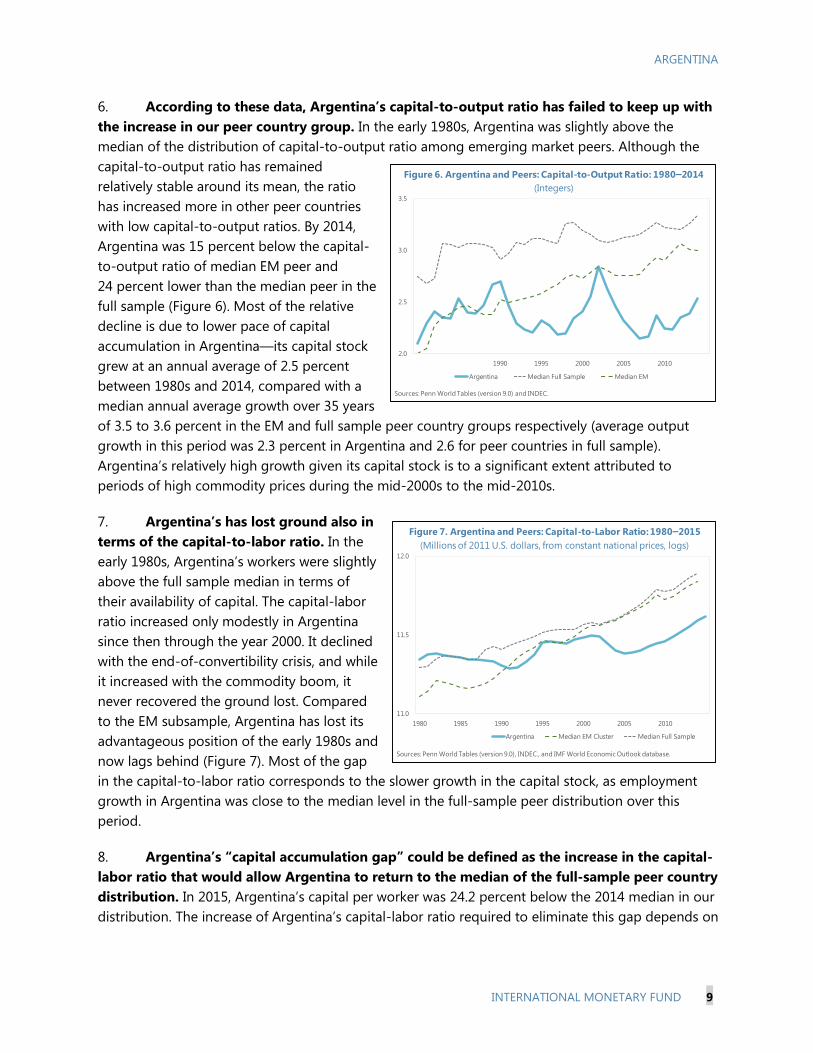
6. According to these data, Argentina’s capital-to-output ratio has failed to keep up with

the increase in our peer country group. In the early 1980s, Argentina was slightly above the

median of the distribution of capital-to-output ratio among emerging market peers. Although the

capital-to-output ratio has remained

relatively stable around its mean, the ratio

has increased more in other peer countries

with low capital-to-output ratios. By 2014,

Argentina was 15 percent below the capital-

to-output ratio of median EM peer and

24 percent lower than the median peer in the

full sample (Figure 6). Most of the relative

decline is due to lower pace of capital

accumulation in Argentina—its capital stock

grew at an annual average of 2.5 percent

between 1980s and 2014, compared with a

median annual average growth over 35 years

of 3.5 to 3.6 percent in the EM and full sample peer country groups respectively (average output

growth in this period was 2.3 percent in Argentina and 2.6 for peer countries in full sample).

Argentina’s relatively high growth given its capital stock is to a significant extent attributed to

periods of high commodity prices during the mid-2000s to the mid-2010s.

7. Argentina’s has lost ground also in

terms of the capital-to-labor ratio. In the

early 1980s, Argentina’s workers were slightly

above the full sample median in terms of

their availability of capital. The capital-labor

ratio increased only modestly in Argentina

since then through the year 2000. It declined

with the end-of-convertibility crisis, and while

it increased with the commodity boom, it

never recovered the ground lost. Compared

to the EM subsample, Argentina has lost its

advantageous position of the early 1980s and

now lags behind (Figure 7). Most of the gap

in the capital-to-labor ratio corresponds to the slower growth in the capital stock, as employment

growth in Argentina was close to the median level in the full-sample peer distribution over this

period.

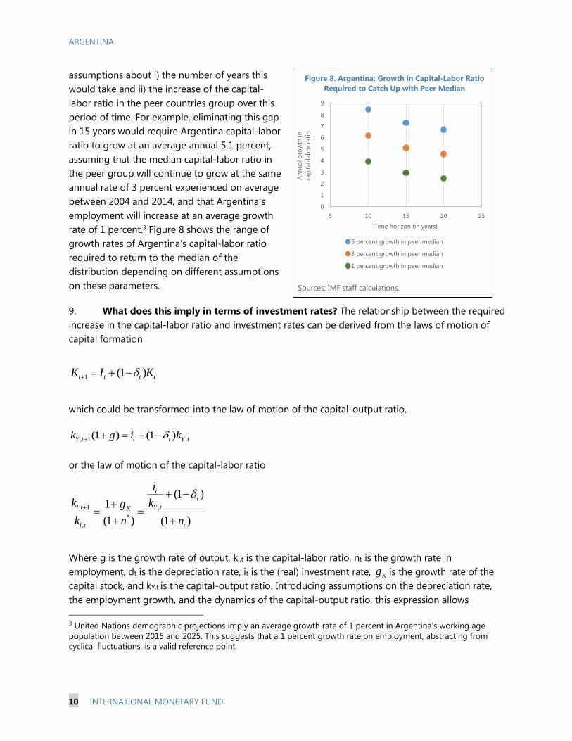
8. Argentina’s “capital accumulation gap” could be defined as the increase in the capital-

labor ratio that would allow Argentina to return to the median of the full-sample peer country

distribution. In 2015, Argentina’s capital per worker was 24.2 percent below the 2014 median in our

distribution. The increase of Argentina’s capital-labor ratio required to eliminate this gap depends on

2.0

2.5

3.0

3.5

1990 1995 2000 2005 2010

Argentina Median Full Sample Median EM

Figure 6. Argentina and Peers: Capital-to-Output Ratio: 1980–2014

(Integers)

Sources: Penn World Tables (version 9.0) and INDEC.

11.0

11.5

12.0

1980 1985 1990 1995 2000 2005 2010

Argentina Median EM Cluster Median Full Sample

Figure 7. Argentina and Peers: Capital-to-Labor Ratio: 1980–2015

(Millions of 2011 U.S. dollars, from constant national prices, logs)

Sources: Penn World Tables (version 9.0), INDEC., and IMF World Economic Outlook database.

ARGENTINA


assumptions about i) the number of years this

would take and ii) the increase of the capital-

labor ratio in the peer countries group over this

period of time. For example, eliminating this gap

in 15 years would require Argentina capital-labor

ratio to grow at an average annual 5.1 percent,

assuming that the median capital-labor ratio in

the peer group will continue to grow at the same

annual rate of 3 percent experienced on average

between 2004 and 2014, and that Argentina’s

employment will increase at an average growth

rate of 1 percent.3 Figure 8 shows the range of

growth rates of Argentina’s capital-labor ratio

required to return to the median of the

distribution depending on different assumptions

on these parameters.

9. What does this imply in terms of investment rates? The relationship between the required

increase in the capital-labor ratio and investment rates can be derived from the laws of motion of

capital formation

1 (1 )t t t tK I K

which could be transformed into the law of motion of the capital-output ratio,

, 1 ,(1 ) (1 )Y t t t Y tk g i k

or the law of motion of the capital-labor ratio

, 1 ,

*

,

(1 )1

(1 ) (1 )

tt

l t Y tK

l t t

i

k kg

k n n

Where g is the growth rate of output, kl,t is the capital-labor ratio, nt is the growth rate in

employment, dt is the depreciation rate, it is the (real) investment rate, Kg is the growth rate of the

capital stock, and kY,t is the capital-output ratio. Introducing assumptions on the depreciation rate,

the employment growth, and the dynamics of the capital-output ratio, this expression allows

3 United Nations demographic projections imply an average growth rate of 1 percent in Argentina’s working age

population between 2015 and 2025. This suggests that a 1 percent growth rate on employment, abstracting from

cyclical fluctuations, is a valid reference point.

0

1

2

3

4

5

6

7

8

9

5 10 15 20 25

An

nu

al g

row

th in

cap

ital-

lab

or

rati

o

Time horizon (in years)

5 percent growth in peer median



Figure 8. Argentina: Growth in Capital-Labor Ratio

Required to Catch Up with Peer Median

Sources: IMF staff calculations.

ARGENTINA


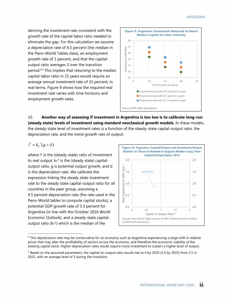
deriving the investment rate consistent with the

growth rate of the capital-labor ratio needed to

eliminate the gap. For this calculation we assume

a depreciation rate of 4.5 percent (the median in

the Penn-World Tables data), an employment

growth rate of 1 percent, and that the capital-

output ratio averages 3 over the transition

period.4,5 This implies that returning to the median

capital-labor ratio in 15 years would require an

average annual investment rate of 32 percent, in

real terms. Figure 9 shows how the required real

investment rate varies with time horizons and

employment growth rates.

10. Another way of assessing if investment in Argentina is too low is to calibrate long-run

(steady state) levels of investment using standard neoclassical growth models. In these models,

the steady-state level of investment rates is a function of the steady-state capital-output ratio, the

depreciation rate, and the trend growth rate of output:

* *( )Yi k g

where i* is the (steady-state) ratio of investment

to real output, kY* is the (steady state) capital-

output ratio, g is potential output growth, and d

is the depreciation rate. We calibrate the

expression linking the steady state investment

rate to the steady state capital-output ratio for all

countries in the peer group, assuming a

4.5 percent depreciation rate (the rate used in the

Penn-World tables to compute capital stocks), a

potential GDP growth rate of 3.3 percent for

Argentina (in line with the October 2016 World

Economic Outlook), and a steady-state capital-

output ratio (kY*) which is the median of the

4 This depreciation rate may be conservative for an economy such as Argentina experiencing a large shift in relative

prices that may alter the profitability of sectors across the economy, and therefore the economic viability of the

existing capital stock. Higher depreciation rates would require more investment to sustain a higher level of output.

5 Based on the assumed parameters, the capital-to-output ratio would rise to 4 by 2030 (3.4 by 2025) from 2.5 in

2015, with an average level of 3 during the transition.

27

29

31

33

35

37

39

5 10 15 20 25

Inve

stm

en

t to

GD

P R

atio

Time horizon (in years)

Employment growth of 0.5 percent a year

Employment growth of 1 percent a year

Employment growth of 1.5 percent a year

Figure 9. Argentina: Investment Required to Reach

Median Capital-to-Labor Intensity

Source: IMF staff calculations.

Figure x. Argentina: Capital/Output and Investment/Output

Relative to Steady-State Level, 2014

Argentina

0.0

0.5

1.0

1.5

2.0

0.0

0.5

1.0

1.5

2.0

0 0.5 1 1.5 2

Real in

vest

men

t to

GD

P r

ati

o *

Capital to Output Ratio *

Figure 10. Argentina: Capital/Output and Investment/Output

Relative to Those to Needed to Support Median Long-Term

Capital/Output Ratio: 2014

Sources: Penn-World Tables (version 9), IMF's World Economic Outlook

and IMF staff calculations.

ARGENTINA


long-run capital-output ratios in peer countries.6 Figure 10 shows that Argentina’s investment rate

and capital-output ratios in 2014 were below these estimated long-run levels. Moving to the long-

run capital-output ratio would require Argentina’s investment rate to be above its steady-state level.

Once the transition is completed, sustaining the steady-state level of the capital-output ratio would

require an investment rate of about 24 percent of GDP.7

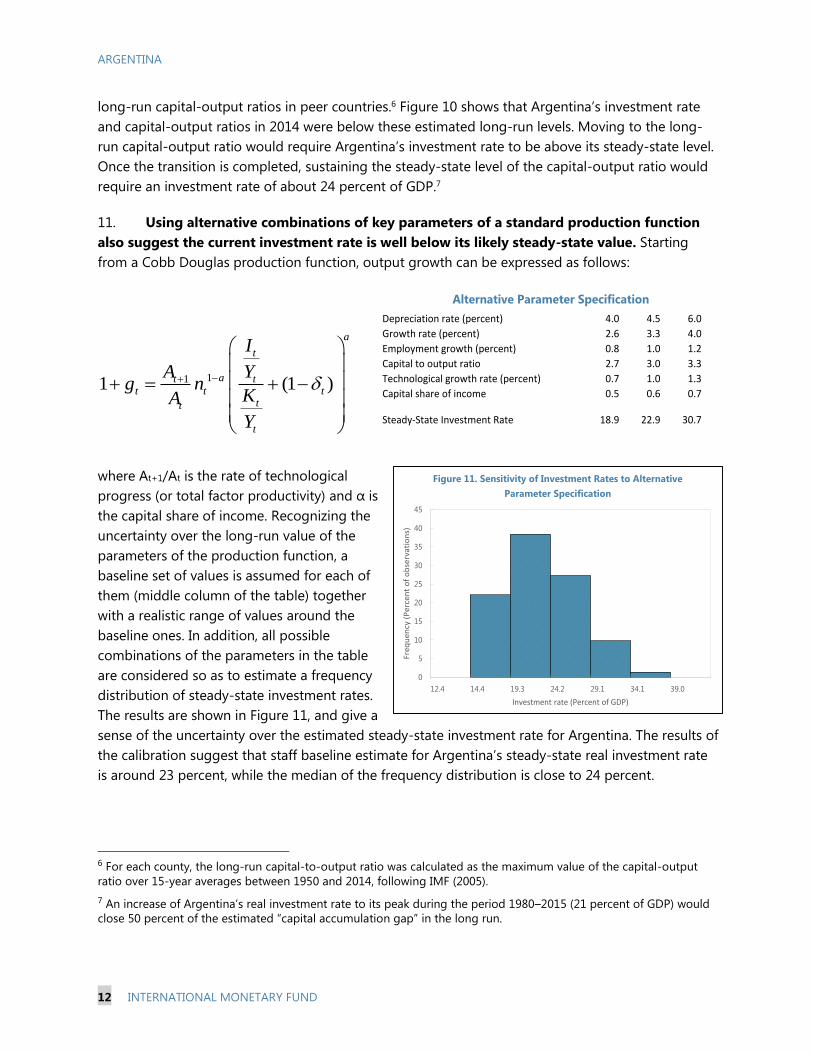
11. Using alternative combinations of key parameters of a standard production function

also suggest the current investment rate is well below its likely steady-state value. Starting

from a Cobb Douglas production function, output growth can be expressed as follows:

where At+1/At is the rate of technological

progress (or total factor productivity) and α is

the capital share of income. Recognizing the

uncertainty over the long-run value of the

parameters of the production function, a

baseline set of values is assumed for each of

them (middle column of the table) together

with a realistic range of values around the

baseline ones. In addition, all possible

combinations of the parameters in the table

are considered so as to estimate a frequency

distribution of steady-state investment rates.

The results are shown in Figure 11, and give a

sense of the uncertainty over the estimated steady-state investment rate for Argentina. The results of

the calibration suggest that staff baseline estimate for Argentina’s steady-state real investment rate

is around 23 percent, while the median of the frequency distribution is close to 24 percent.

6 For each county, the long-run capital-to-output ratio was calculated as the maximum value of the capital-output

ratio over 15-year averages between 1950 and 2014, following IMF (2005).

7 An increase of Argentina’s real investment rate to its peak during the period 1980–2015 (21 percent of GDP) would

close 50 percent of the estimated “capital accumulation gap” in the long run.

111 (1 )

a

t

at tt t t

tt

t

I

A Yg n

KA

Y

Depreciation rate (percent) 4.0 4.5 6.0

Growth rate (percent) 2.6 3.3 4.0

Employment growth (percent) 0.8 1.0 1.2

Capital to output ratio 2.7 3.0 3.3

Technological growth rate (percent) 0.7 1.0 1.3

Capital share of income 0.5 0.6 0.7

Steady-State Investment Rate 18.9 22.9 30.7

Alternative Parameter Specification

Figure 11. Sensitivity of Investment Rates to Alternative

Parameter Specification

0

5

10

15

20

25

30

35

40

45

12.4 14.4 19.3 24.2 29.1 34.1 39.0

Fre

qu

en

cy (

Pe

rce

nt

of

ob

serv

atio

ns)

Investment rate (Percent of GDP)

ARGENTINA


12. Argentina’s capital accumulation gap with respect to its peers is evident when it comes

to infrastructure. Electricity production and access to electricity is significantly lower. Argentina

ranks in the low 12 percent in access to electricity and 30 percent in production of electricity among

its peers. On both of these counts, Argentina has declined since the 1990s. It ranks better in the

production of energy, an area where it has improved with the discoveries of energy resources in the

period. The quality of trade and transport related infrastructure is also relatively low. On

communications, the picture is mixed. Argentina ranks relatively high on cell phone penetration, but

ranks below the median on internet access (Figure 12).

Figure 12. Argentina Infrastructure Indicators: Argentina’s Percentile in

Distribution of Peer Advanced and Emerging Markets

13. If Argentina’s investment rate were to increase, what would be the impact on output?

While there is a vast literature on the link between investment and output, there is a great range of

estimates on the impact of an exogenous investment shock on GDP growth, Among the others,

Barro (1991), Barro and Lee (1993), Houthakker (1961), Modigliani (1970) and Carroll and Weil (1994)

all find a positive association between investment and growth using growth-regression and cross-

section studies. In this section we customize our empirical analysis to Argentina’s peer group using

two separate methodologies:

A panel regression that directly relates the increase in investment rates to GDP growth, and thus

provides an empirical estimate of the investment accelerator effects. Because the answer may

vary with the time horizon, we estimate the panel relationship over five- and ten-year

Energy production

Energy production per person

Electricity production (kWh per person)

Access to electricity (% of population)

Transportation

Rail lines (total route-km per person)

Quality of trade and transport-related infrastructure (1=low to 5=high)

Quality of port infrastructure, WEF (1=extremely underdeveloped to 7=well

developed and efficient by international standards)Communications

Mobile cellular subscriptions (per 100 people)

Internet users (per 100 people)

Fixed broadband Internet subscribers (per 100 people)

Others

Hospitals per 1000 individuals

Improved water source (% of population with access)

0 10 20 30 40 50 60 70 80 90 100

1

2

3

4

5

6

7

8

9

10

11

12

13

14

15

1990 2000 2010

Figure 12. Argentina Infrastructure Indicators: Argentina’s Percentile in Distribution of Peer

Advanced and Emerging Markets

Source: World Bank's World Development Indicators database.

ARGENTINA


frequencies, (see Annex I). The exercise controls for growth in relative export prices, deviations of

the real exchange rate from its long-term average, fiscal balances to GDP, and net foreign direct

investment to GDP.

A production function approach, that measures the impact of an increase of the capital-labor

ratios on output per worker. This allows us to determine the impact on potential (long-term)

growth from filling the capital accumulation gap, controlling for country specific demographic

factors, labor market developments and relative export prices (Annex II).

14. We find that a 1 percentage point permanent increase in the investment rate could

increase annual output growth between 0.1 and 0.3 percentage points.

The panel regressions suggest that a one percentage point increase in the investment rate over a

5 or 10-year period would raise GDP growth by an annual average of about 0.1 percentage

points over the same period. The panel regression also shows that increases in relative export

prices, a depreciation of the real exchange rate, and stronger fiscal balances all have positive

effects on growth.

The production function approach yields that for each percentage point increase in the capital-

labor ratio, output per worker would increases by 0.6 percentage points. This estimated

parameter can be interpreted as the capital share of income (α) in a Cobb Douglas production

function shown above. Based on the calibration of the production function described by the

mid-column of the previous Table, a (permanent) increase in the investment rate by

1 percentage point would raise potential growth by about 0.3 percent.

C. What Drives Investment Surges? An Event Analysis

15. In this section, we focus our attention on past episodes of persistent investment

surges. The objective is to identify the stylized behavior of key macroeconomic and financial

variables during those episodes, so as to infer under what conditions a surge in investment would

likely take place in Argentina over the coming years and what could the Argentine authorities do to

increase the likelihood of such a surge taking place. Investment surges episodes are identified as

periods in which the three-year moving average of investment rates (share of nominal GDP)

increases by at least 2 percent of GDP. The “duration” of each episode is the number of years

between the troughs and peaks of the investment series, whereas the “size” of each episode is the

trough-peak increase.

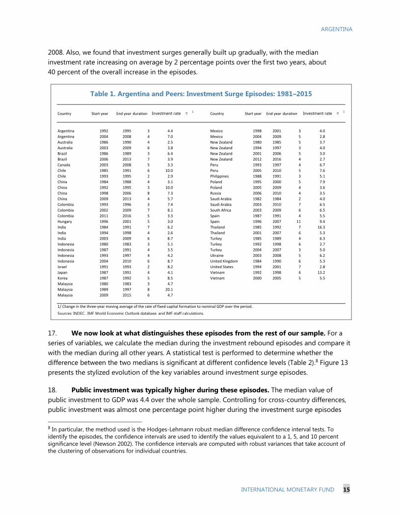
16. In general, investment surges took place over a number of years. We found 57 episodes

in our sample (Table 1) with an average duration of 4.8 years and an average size of 5.9 percent of

GDP (a median duration of 5 years for a median increase of the investment rate of 5.1 percentage

points of GDP). The longest episode took place in Spain between 1996 and 2007. Argentina

experienced two surges. The first took place at the beginning of the convertibility period between

1992 and 1995. The second one right started in 2004 and ended with the global financial crisis in

ARGENTINA


2008. Also, we found that investment surges generally built up gradually, with the median

investment rate increasing on average by 2 percentage points over the first two years, about

40 percent of the overall increase in the episodes.

Table 1. Argentina and Peers: Investment Surge Episodes: 1981–2015

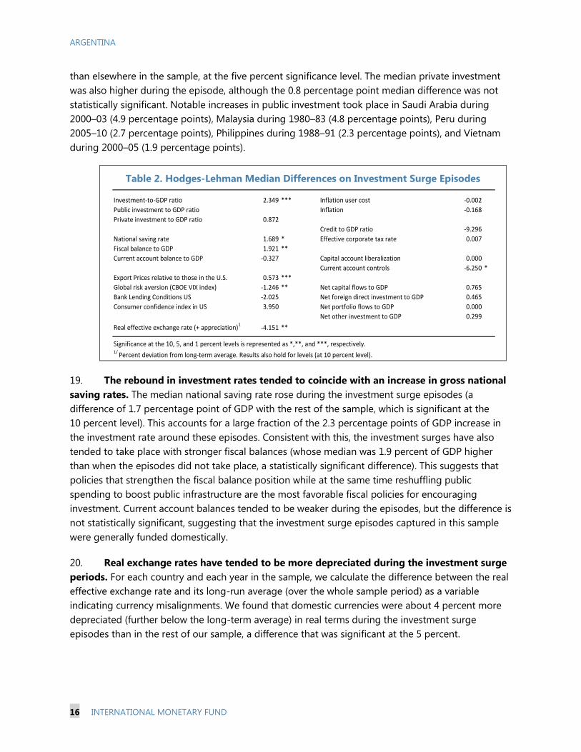
17. We now look at what distinguishes these episodes from the rest of our sample. For a

series of variables, we calculate the median during the investment rebound episodes and compare it

with the median during all other years. A statistical test is performed to determine whether the

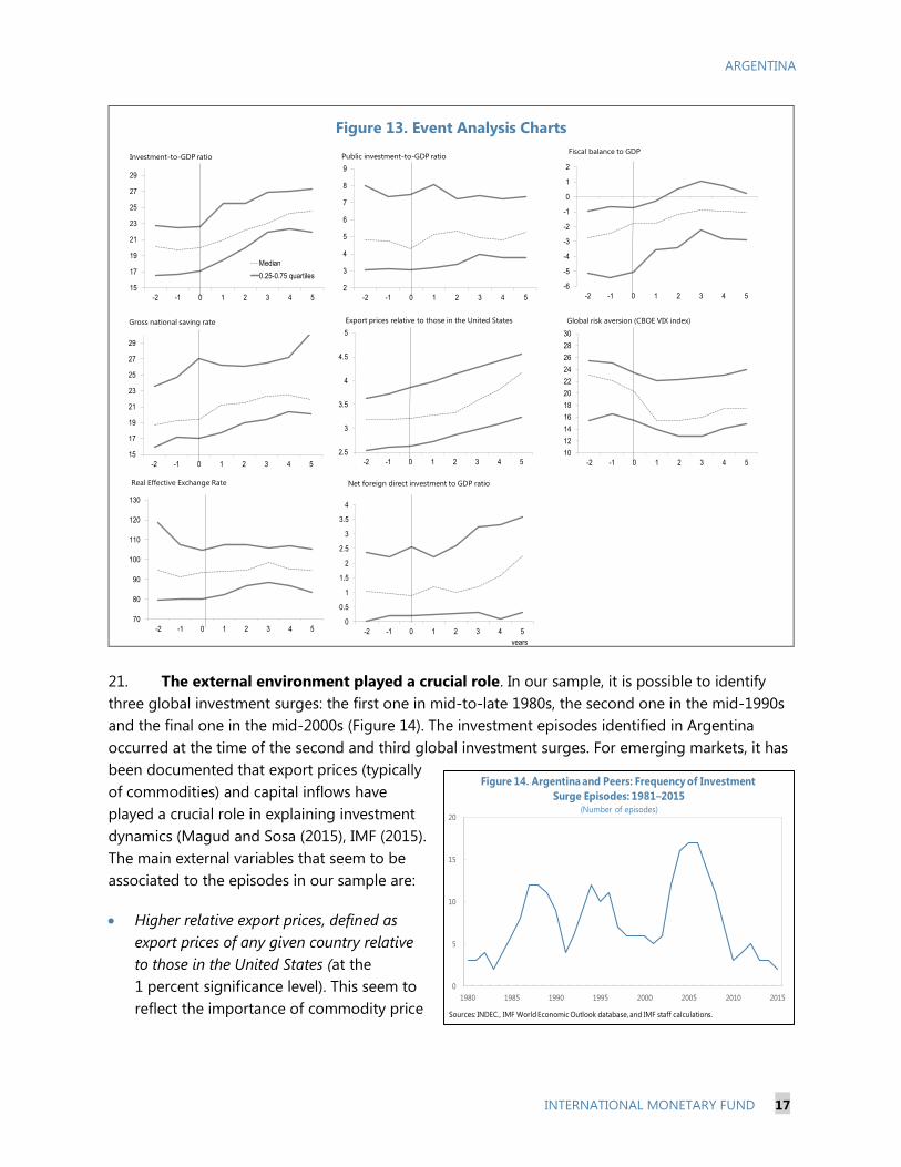
difference between the two medians is significant at different confidence levels (Table 2).8 Figure 13

presents the stylized evolution of the key variables around investment surge episodes.

18. Public investment was typically higher during these episodes. The median value of

public investment to GDP was 4.4 over the whole sample. Controlling for cross-country differences,

public investment was almost one percentage point higher during the investment surge episodes

8 In particular, the method used is the Hodges-Lehmann robust median difference confidence interval tests. To

identify the episodes, the confidence intervals are used to identify the values equivalent to a 1, 5, and 10 percent

significance level (Newson 2002). The confidence intervals are computed with robust variances that take account of

the clustering of observations for individual countries.

Country Start year End year duration Investment rate D 1

Country Start year End year duration Investment rate D 1

Argentina 1992 1995 3 4.4 Mexico 1998 2001 3 4.0

Argentina 2004 2008 4 7.0 Mexico 2004 2009 5 2.8

Australia 1986 1990 4 2.5 New Zealand 1980 1985 5 3.7

Australia 2003 2009 6 3.8 New Zealand 1994 1997 3 4.0

Brazil 1986 1989 3 6.4 New Zealand 2001 2006 5 3.0

Brazil 2006 2013 7 3.9 New Zealand 2012 2016 4 2.7

Canada 2003 2008 5 3.3 Peru 1993 1997 4 6.7

Chile 1985 1991 6 10.0 Peru 2005 2010 5 7.6

Chile 1993 1995 2 2.9 Philippines 1988 1991 3 5.1

China 1984 1988 4 3.1 Poland 1995 2000 5 7.9

China 1992 1995 3 10.0 Poland 2005 2009 4 3.6

China 1998 2006 8 7.3 Russia 2006 2010 4 3.5

China 2009 2013 4 5.7 Saudi Arabia 1982 1984 2 4.0

Colombia 1993 1996 3 7.4 Saudi Arabia 2003 2010 7 6.5

Colombia 2002 2009 7 8.1 South Africa 2003 2009 6 6.5

Colombia 2011 2016 5 3.3 Spain 1987 1991 4 5.5

Hungary 1996 2001 5 3.0 Spain 1996 2007 11 9.4

India 1984 1991 7 6.2 Thailand 1985 1992 7 16.3

India 1994 1998 4 2.6 Thailand 2001 2007 6 5.3

India 2003 2009 6 8.7 Turkey 1985 1989 4 6.3

Indonesia 1980 1983 3 5.1 Turkey 1992 1998 6 2.7

Indonesia 1987 1991 4 3.5 Turkey 2004 2007 3 5.0

Indonesia 1993 1997 4 4.2 Ukraine 2003 2008 5 6.2

Indonesia 2004 2010 6 8.7 United Kingdom 1984 1990 6 5.3

Israel 1991 1993 2 8.2 United States 1994 2001 7 2.8

Japan 1987 1991 4 4.1 Vietnam 1992 1998 6 13.2

Korea 1987 1992 5 8.5 Vietnam 2000 2005 5 5.5

Malaysia 1980 1983 3 4.7

Malaysia 1989 1997 8 20.1

Malaysia 2009 2015 6 4.7

1/ Change in the three-year moving average of the rate of fixed capital formation to nominal GDP over the period.

Sources: INDEC., IMF World Economic Outlook database, and IMF staff calculations.

ARGENTINA


than elsewhere in the sample, at the five percent significance level. The median private investment

was also higher during the episode, although the 0.8 percentage point median difference was not

statistically significant. Notable increases in public investment took place in Saudi Arabia during

2000–03 (4.9 percentage points), Malaysia during 1980–83 (4.8 percentage points), Peru during

2005–10 (2.7 percentage points), Philippines during 1988–91 (2.3 percentage points), and Vietnam

during 2000–05 (1.9 percentage points).

Table 2. Hodges-Lehman Median Differences on Investment Surge Episodes

19. The rebound in investment rates tended to coincide with an increase in gross national

saving rates. The median national saving rate rose during the investment surge episodes (a

difference of 1.7 percentage point of GDP with the rest of the sample, which is significant at the

10 percent level). This accounts for a large fraction of the 2.3 percentage points of GDP increase in

the investment rate around these episodes. Consistent with this, the investment surges have also

tended to take place with stronger fiscal balances (whose median was 1.9 percent of GDP higher

than when the episodes did not take place, a statistically significant difference). This suggests that

policies that strengthen the fiscal balance position while at the same time reshuffling public

spending to boost public infrastructure are the most favorable fiscal policies for encouraging

investment. Current account balances tended to be weaker during the episodes, but the difference is

not statistically significant, suggesting that the investment surge episodes captured in this sample

were generally funded domestically.

20. Real exchange rates have tended to be more depreciated during the investment surge

periods. For each country and each year in the sample, we calculate the difference between the real

effective exchange rate and its long-run average (over the whole sample period) as a variable

indicating currency misalignments. We found that domestic currencies were about 4 percent more

depreciated (further below the long-term average) in real terms during the investment surge

episodes than in the rest of our sample, a difference that was significant at the 5 percent.

Investment-to-GDP ratio 2.349 *** Inflation user cost -0.002

Public investment to GDP ratio Inflation -0.168

Private investment to GDP ratio 0.872

Credit to GDP ratio -9.296

National saving rate 1.689 * Effective corporate tax rate 0.007

Fiscal balance to GDP 1.921 **

Current account balance to GDP -0.327 Capital account liberalization 0.000

Current account controls -6.250 *

Export Prices relative to those in the U.S. 0.573 ***

Global risk aversion (CBOE VIX index) -1.246 ** Net capital flows to GDP 0.765

Bank Lending Conditions US -2.025 Net foreign direct investment to GDP 0.465

Consumer confidence index in US 3.950 Net portfolio flows to GDP 0.000

Net other investment to GDP 0.299

Real effective exchange rate (+ appreciation)1-4.151 **

Significance at the 10, 5, and 1 percent levels is represented as *,**, and ***, respectively. 1/ Percent deviation from long-term average. Results also hold for levels (at 10 percent level).

Table 2. Hodges-Lehmann median differences on Investment Surge Episodes

ARGENTINA


Figure 13. Event Analysis Charts

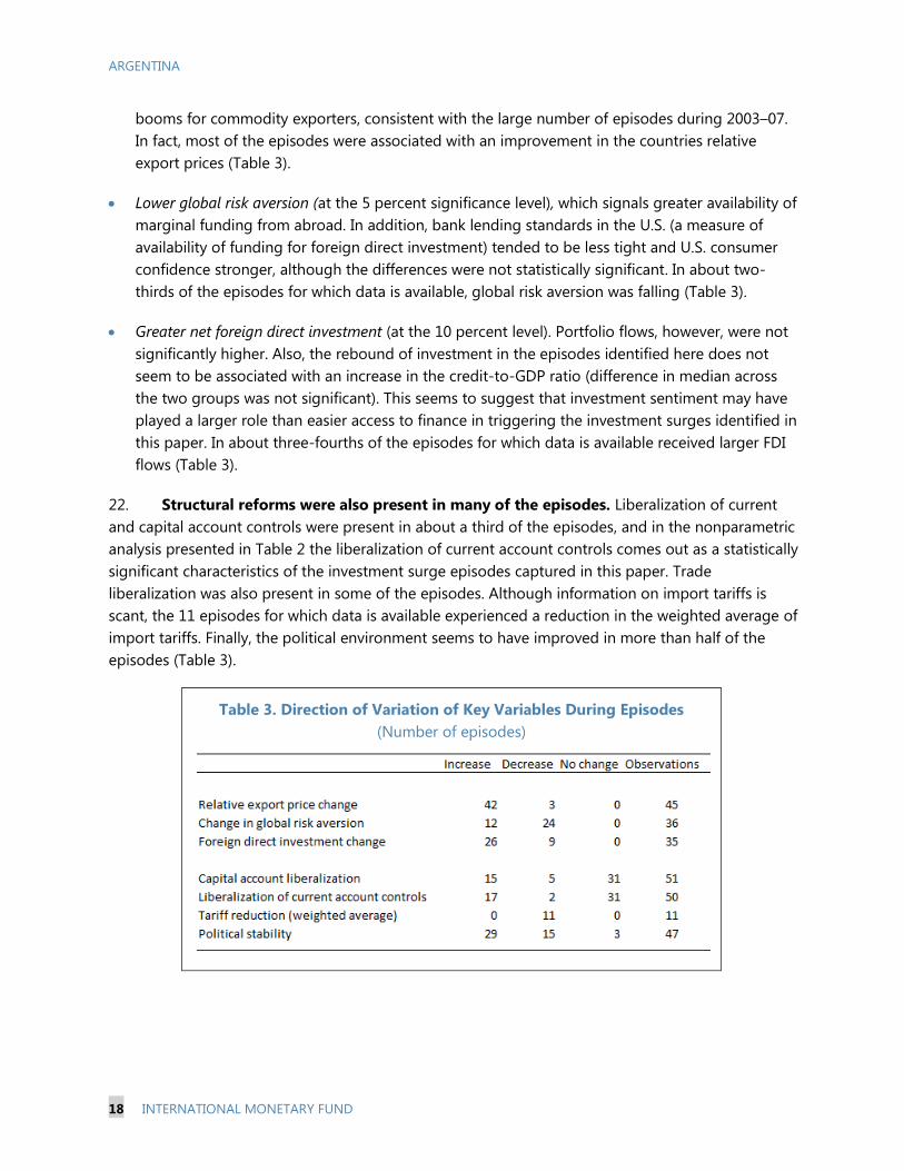
21. The external environment played a crucial role. In our sample, it is possible to identify

three global investment surges: the first one in mid-to-late 1980s, the second one in the mid-1990s

and the final one in the mid-2000s (Figure 14). The investment episodes identified in Argentina

occurred at the time of the second and third global investment surges. For emerging markets, it has

been documented that export prices (typically

of commodities) and capital inflows have

played a crucial role in explaining investment

dynamics (Magud and Sosa (2015), IMF (2015).

The main external variables that seem to be

associated to the episodes in our sample are:

Higher relative export prices, defined as

export prices of any given country relative

to those in the United States (at the

1 percent significance level). This seem to

reflect the importance of commodity price

-2 -1 0 1 2 3 4 5

Figure 13. Event Analysis Charts

15

17

19

21

23

25

27

29

-2 -1 0 1 2 3 4 5

Median

0.25-0.75 quartiles

2

3

4

5

6

7

8

9

-2 -1 0 1 2 3 4 5

Investment-to-GDP ratio Public investment-to-GDP ratio

-6

-5

-4

-3

-2

-1

0

1

2

-2 -1 0 1 2 3 4 5

Fiscal balance to GDP

15

17

19

21

23

25

27

29

-2 -1 0 1 2 3 4 5

Gross national saving rate

2.5

3

3.5

4

4.5

5

-2 -1 0 1 2 3 4 510

12

14

16

18

20

22

24

26

28

30

-2 -1 0 1 2 3 4 5

Global risk aversion (CBOE VIX index)Export prices relative to those in the United States

70

80

90

100

110

120

130

-2 -1 0 1 2 3 4 50

0.5

1

1.5

2

2.5

3

3.5

4

-2 -1 0 1 2 3 4 5

years

Real Effective Exchange Rate Net foreign direct investment to GDP ratio

0

5

10

15

20

1980 1985 1990 1995 2000 2005 2010 2015

Figure 14. Argentina and Peers: Frequency of Investment

Surge Episodes: 1981–2015(Number of episodes)

Sources: INDEC., IMF World Economic Outlook database, and IMF staff calculations.

ARGENTINA


booms for commodity exporters, consistent with the large number of episodes during 2003–07.

In fact, most of the episodes were associated with an improvement in the countries relative

export prices (Table 3).

Lower global risk aversion (at the 5 percent significance level), which signals greater availability of

marginal funding from abroad. In addition, bank lending standards in the U.S. (a measure of

availability of funding for foreign direct investment) tended to be less tight and U.S. consumer

confidence stronger, although the differences were not statistically significant. In about two-

thirds of the episodes for which data is available, global risk aversion was falling (Table 3).

Greater net foreign direct investment (at the 10 percent level). Portfolio flows, however, were not

significantly higher. Also, the rebound of investment in the episodes identified here does not

seem to be associated with an increase in the credit-to-GDP ratio (difference in median across

the two groups was not significant). This seems to suggest that investment sentiment may have

played a larger role than easier access to finance in triggering the investment surges identified in

this paper. In about three-fourths of the episodes for which data is available received larger FDI

flows (Table 3).

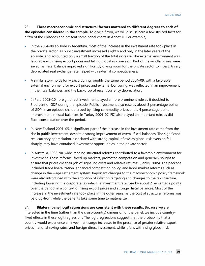
22. Structural reforms were also present in many of the episodes. Liberalization of current

and capital account controls were present in about a third of the episodes, and in the nonparametric

analysis presented in Table 2 the liberalization of current account controls comes out as a statistically

significant characteristics of the investment surge episodes captured in this paper. Trade

liberalization was also present in some of the episodes. Although information on import tariffs is

scant, the 11 episodes for which data is available experienced a reduction in the weighted average of

import tariffs. Finally, the political environment seems to have improved in more than half of the

episodes (Table 3).

Table 3. Direction of Variation of Key Variables During Episodes

(Number of episodes)

ARGENTINA


23. These macroeconomic and structural factors mattered to different degrees to each of

the episodes considered in the sample. To give a flavor, we will discuss here a few stylized facts for

a few of the episodes and present some panel charts in Annex III. For example,

In the 2004–08 episode in Argentina, most of the increase in the investment rate took place in

the private sector, as public investment increased slightly and only in the later years of the

episode, and accounted only a small fraction of the total increase. The external environment was

favorable with rising export prices and falling global risk aversion. Part of the windfall gains were

saved, as fiscal balance improved significantly giving room for the private sector to invest. A very

depreciated real exchange rate helped with external competitiveness.

A similar story holds for Mexico during roughly the same period 2004–09, with a favorable

external environment for export prices and external borrowing, was reflected in an improvement

in the fiscal balances, and the backdrop of recent currency depreciation.

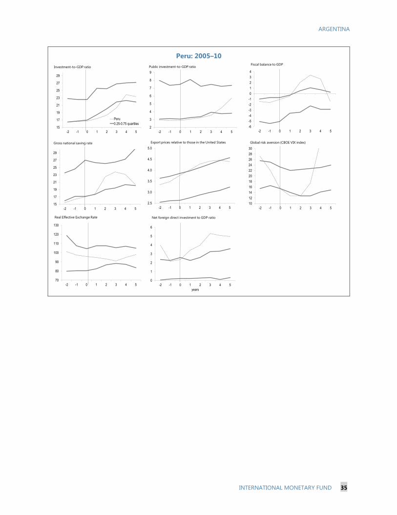
In Peru 2005–10, foreign direct investment played a more prominent role as it doubled to

5 percent of GDP during the episode. Public investment also rose by about 3 percentage points

of GDP, in an episode characterized by rising commodity prices and a 4 percentage point

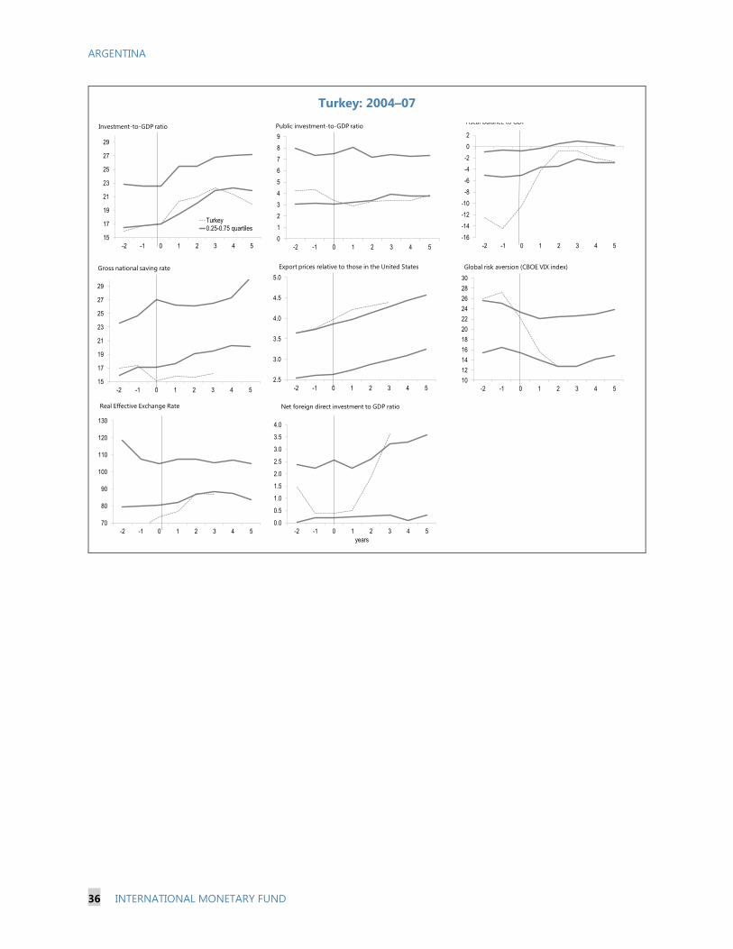
improvement in fiscal balances. In Turkey 2004–07, FDI also played an important role, as did

fiscal consolidation over the period.

In New Zealand 2001–05, a significant part of the increase in the investment rate came from the

rise in public investment, despite a strong improvement of overall fiscal balances. The significant

real currency appreciation, associated with strong capital inflows as global risk aversion fell

sharply, may have contained investment opportunities in the private sector.

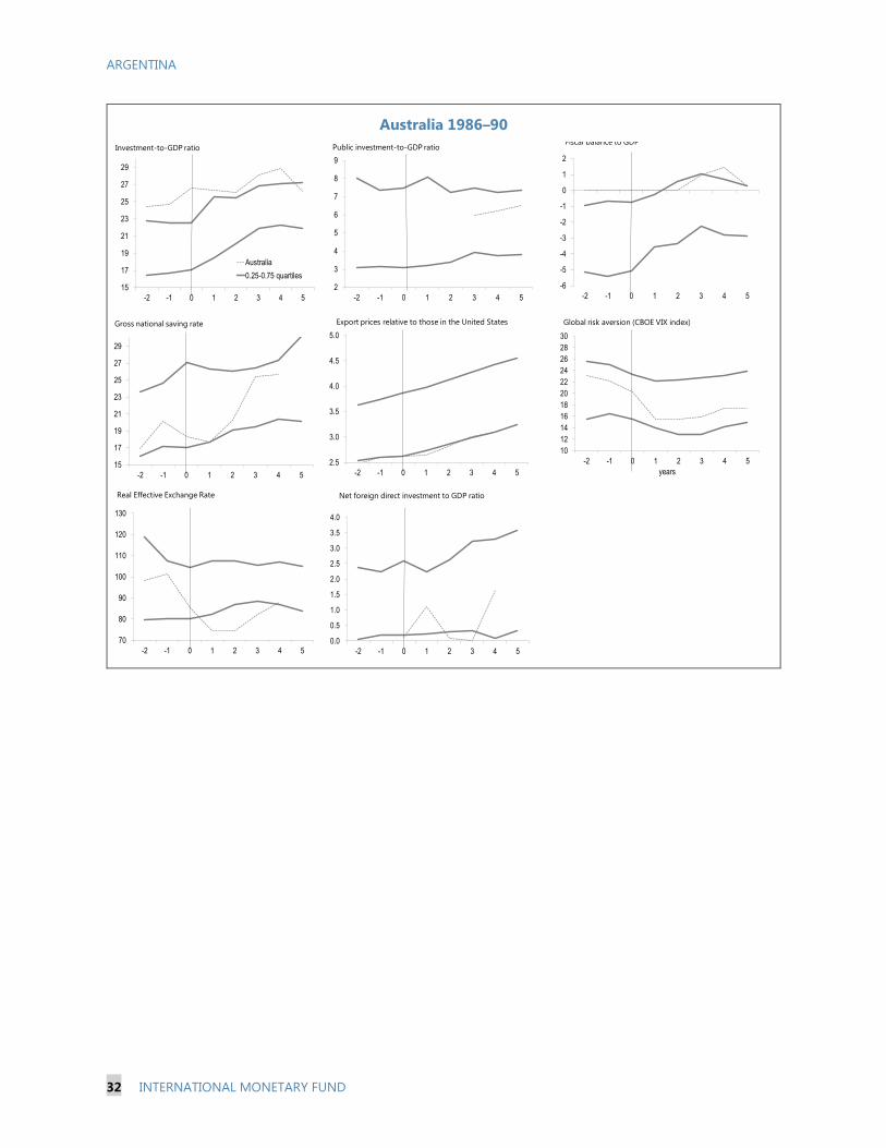
In Australia, 1986–90, wide-ranging structural reforms contributed to a favorable environment for

investment. These reforms “freed up markets, promoted competition and generally sought to

ensure that prices did their job of signaling costs and relative returns” (Banks, 2005). The package

included trade liberalization, enhanced competition policy, and labor market reforms such as

change in the wage settlement system. Important changes to the macroeconomic policy framework

were also introduced with the adoption of inflation targeting and changes to the tax structure,

including lowering the corporate tax rate. The investment rate rose by about 2 percentage points

over the period, in a context of rising export prices and stronger fiscal balances. Most of the

increase in the investment rate took place in the outer years, as the cost of structural reforms was

paid up-front while the benefits take some time to materialize.

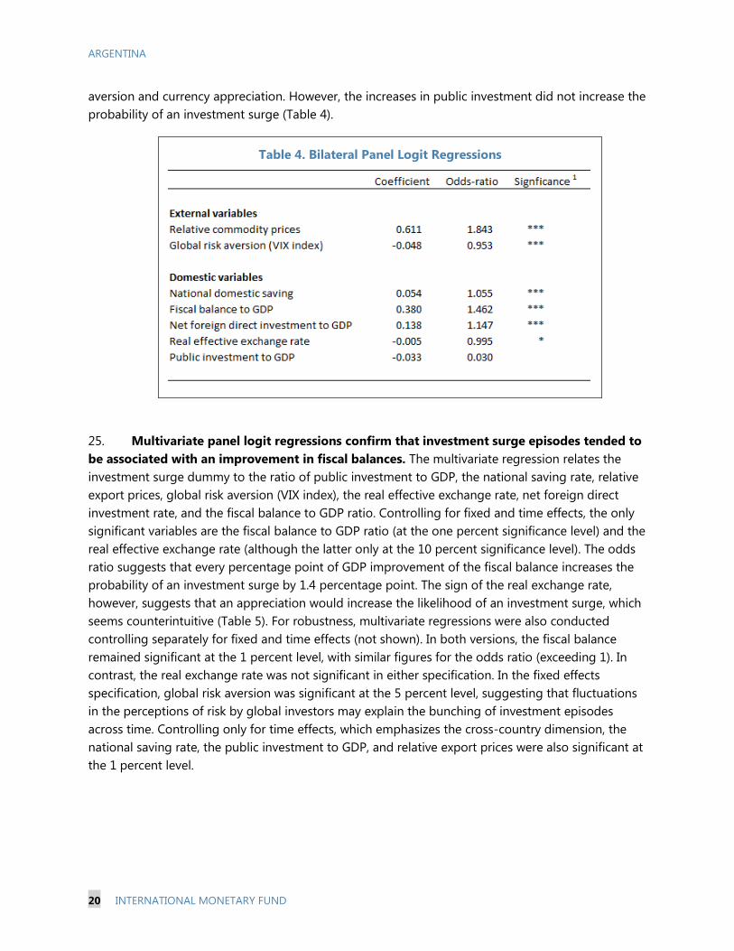
24. Bilateral panel logit regressions are consistent with these results. Because we are

interested in the time (rather than the cross-country) dimension of the panel, we include country-

fixed effects in these logit regressions The logit regressions suggest that the probability that a

country would experience an investment surge increases in the presence of greater relative export

prices, national saving rates, and foreign direct investment, while it falls with rising global risk

ARGENTINA


aversion and currency appreciation. However, the increases in public investment did not increase the

probability of an investment surge (Table 4).

Table 4. Bilateral Panel Logit Regressions

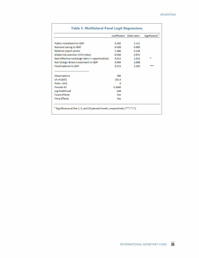
25. Multivariate panel logit regressions confirm that investment surge episodes tended to

be associated with an improvement in fiscal balances. The multivariate regression relates the

investment surge dummy to the ratio of public investment to GDP, the national saving rate, relative

export prices, global risk aversion (VIX index), the real effective exchange rate, net foreign direct

investment rate, and the fiscal balance to GDP ratio. Controlling for fixed and time effects, the only

significant variables are the fiscal balance to GDP ratio (at the one percent significance level) and the

real effective exchange rate (although the latter only at the 10 percent significance level). The odds

ratio suggests that every percentage point of GDP improvement of the fiscal balance increases the

probability of an investment surge by 1.4 percentage point. The sign of the real exchange rate,

however, suggests that an appreciation would increase the likelihood of an investment surge, which

seems counterintuitive (Table 5). For robustness, multivariate regressions were also conducted

controlling separately for fixed and time effects (not shown). In both versions, the fiscal balance

remained significant at the 1 percent level, with similar figures for the odds ratio (exceeding 1). In

contrast, the real exchange rate was not significant in either specification. In the fixed effects

specification, global risk aversion was significant at the 5 percent level, suggesting that fluctuations

in the perceptions of risk by global investors may explain the bunching of investment episodes

across time. Controlling only for time effects, which emphasizes the cross-country dimension, the

national saving rate, the public investment to GDP, and relative export prices were also significant at

the 1 percent level.

ARGENTINA


Table 5. Multilateral Panel Logit Regressions

ARGENTINA


References

Aghion, P., Comin, D. and Howitt, P. (2006), “When Does Domestic Saving Matter for Economic

Growth?” NBER Working Paper No. 12275.

Banks, Gary, 2005, Structural reform Australian-style: lessons for others? Presentation to the

IMF/World Bank (Washington DC, 26–27 May 2005) and OECD (Paris, 31 May 2005), Productivity

Commission, Canberra, +May.

Barro, R. J. (1991), “Economic Growth in a Cross Section of Countries,” The Quarterly Journal of

Economics, 106, pp. 407–43.

Barro, R. J., and J. W. Lee (1993) “International Comparisons of Educational Attainment,” Journal of

Monetary Economics, Vol. 32, 363–394.

Bradbury, Mathew, 2013, “Estimating Potential Output: Argentina 2003-2011, Medium Term

Quarterly Calculations of the Production Function,” Queens College, CUNY, Working Paper

Draft

Carroll, Christopher D., and David N. Weil, (1994), “Saving and Growth: A Reinterpretation,”

Carnegie-Rochester Conference Series on Public Policy, No. 40, pp. 133–92.

Cheung, Yin-Wong, Michael P. Dooley, and Vladyslav Sushko, 2012, “Investment and Growth in Rich

and Poor Countries,” NBER Working Paper 17788, electronically available at

http://www.nber.org/papers/w17788.

The Conference Board. 2015. The Conference Board Total Economy Database™, September 2015,

http://www.conference-board.org/data/economydatabase/

Coremberg, Ariel, 2008, “The Measurement of TFP in Argentina, 1990–2004: A Case of the Tyranny of

Numbers, Economic Cycles and Methodology, United Nations Economic Commission for

Latin America and the Caribbean.

Coremberg, Ariel, 2011, “The Argentine Productivity Slowdown. The challenges after global financial

collapse. World Economics, Vol 12. No3 (July–September).

Coremberg, Ariel, 2012, “Measuring Productivity in Unstable and Natural Resources Dependent

Economies: Argentina,” Second World KLEMS Conference Harvard University Cambridge,

Massachusetts (August 9–10).

Coremberg, Ariel, 2014, “Measuring Argentina's GDP: Myths And Facts,” World Economics, Vol 15.

No1 (January–March).

http://www.conference-board.org/data/economydatabase/

ARGENTINA


Elosegui, P., Garegnani, L., Lanteri, L., Lepone, F. y Sotes Paladino, J. (2006), “Estimaciones

Alternativas de la Brecha del Producto para la Economía Argentina”. Ensayos Económicos N°

45, Banco Central de la República Argentina.

Escudé, Guillermo, Ma. Florencia Gabrielli, Luis N. Lanteri, and Ma. Josefina Rouillet, 2004,

“Estimating Potential Output For Argentina: 1980.1 - 2004.1 1,” Central Bank of Argentina,

Economic and Financial Research Department.

Robert C. Feenstra, Robert Inklaar. Marcel Timmer (2013). “The Next Generation of the Penn World

Table,” NBER Working Paper no. 19255

Hofman, André A. and Heriberto Tapia, 2003, “Potential output in Latin America: a standard

approach for the 1950-2002 period,” CEPAL, Serie Estudios Estadisticos y Prospectivos 25.

Electronically available here.

Houthakker, Hendrik S. (1961), “An International Comparison of Personal Savings,” Bulletin of the

International Statistical Institute, No. 38, pp. 55–69.

International Monetary Fund, 2005, “Global Imbalances: A Saving and Investment Perspective,” in

World Economic Outlook (September, Box 2.4)

International Monetary Fund, 2015a, “Where Are We Headed? Perspectives on Potential Output,”

World Economic Outlook, April 2015, Chapter 3.

International Monetary Fund, 2015b, “Recent Investment Weakness in Latin America, Is there a

Puzzle?” in Western Hemisphere Regional Economic Outlook (April).

International Monetary Fund, 2015c, “Estimating Public, Private, and PPP Capital Stocks,” in Making

Investment More Efficient (IMF Board Paper), available for download at

http://www.imf.org/external/np/fad/publicinvestment/data/info.pdf.

International Monetary Fund, forthcoming, “Structural Reforms and Macroeconomic Performance:

Initial Considerations for the Fund,” IMF Policy Paper. Electronically available at

http://www.imf.org/external/pp/ppindex.aspx

Lee, Il Houng, Murtaza Syed, and Liu Xueyan, 2012, “Is China Over-Investing and Does it Matter?”

IMF Working Paper No. WP/12/277.

Magud, Nicolas and Leandro Medina, 2011, “The Chilean Output Gap,” IMF Working Paper No.

WP/11/2.

Magud; Nicolas E. and Sebastian Sosa, 2015, ‘Investment in Emerging Markets We Are Not in Kansas

Anymore…Or Are We?” IMF Working Paper No. 15/77.

http://repositorio.cepal.org/bitstream/handle/11362/4721/S2003726_en.pdf?sequence=1

http://www.imf.org/external/np/fad/publicinvestment/data/info.pdf

http://www.imf.org/external/pp/ppindex.aspx

ARGENTINA


Maia, J. y Nicholson, P. (2001), “El Stock de Capital y la Productividad Total de los Factores en la

Argentina”. Dirección Nacional de Coordinación de Políticas Macroeconómicas, Argentina.

Maia, José Luis and Mercedes Kweitel, 2003, “Argentina: Sustainable Output Growth after the

Collapse” Ministerio de Economía-Argentina, Dirección Nacional de Políticas

Macroeconómicas.

Meloni, O. (1999), “Crecimiento Potencial y Productividad en la Argentina: 1980–1997”, en Anales de

la Asociación Argentina de Economía Política.

Newson, R. 2002. Parameters behind “nonparametric” statistics: Kendall’s tau, Somers’ D and median

differences. Stata Journal 2: 45–64.

Rodríguez, José María, 2007, “El Producto Potencial de la Argentina,” Universidad Nacional de

Córdoba.

Taylor, Alan M., 2014, “The Argentina Paradox: Microexplanations and Macropuzzles,” NBER Working

Paper No. 19924 (February).

ARGENTINA


Annex I. Panel Investment and Growth

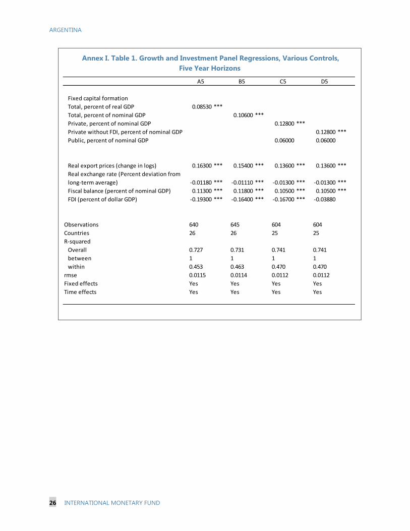
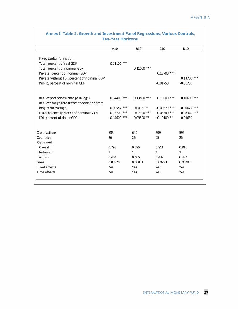
The international experience on the relationship between investment and growth can be

summarized through a panel regression. The unbalanced panel is estimated for the period 1980–

2014 controlling for growth in relative export prices as well as for fixed and time effects. Two

versions of the panel are estimated to assess the relevance of how long an increase in the potential

capital formation rate is sustained: 5 years, and 10 years. For example, the interpretation of the

coefficient on the real investment (fixed capital formation) rate in the 10-year version of the panel

would be that a 1 percentage point increase in the fixed capital formation rate sustained for 10 years

would deliver an annual percent increase of 0.0954 percent. Over ten years, this would imply about a

1 percent increase in GDP.

The results are robust to different versions of the capital formation ratio and the inclusion of

additional controls, including the real exchange rate deviations from long-run trends, the fiscal

balance to GDP and foreign direct investment (FDI) in percent of GDP. The impact of commodity

prices, however declines, suggesting that commodity prices may in turn affect the other controls,

like the real exchange rate, fiscal balances, and even FDI. The difference in the growth impact of

fixed capital formation when expressed as percent of nominal or real GDP virtually disappears at the

10 year frequencies. The estimates suggest that real exchange rate appreciation hurts economic

growth (perhaps through competitiveness considerations) as do fiscal deficits sustained over 5 to

10 year horizons (perhaps through crowding out of the private sector). The results also suggest that

private investment is more important than public investment in growth fluctuations, and that non-

FDI funded fixed capital formation has a stronger impact than FDI on economic activity, perhaps

through lower import leakages.

ARGENTINA


Annex I. Table 1. Growth and Investment Panel Regressions, Various Controls,

Five Year Horizons

A5 B5 C5 D5

Fixed capital formation

Total, percent of real GDP 0.08530 ***

Total, percent of nominal GDP 0.10600 ***

Private, percent of nominal GDP 0.12800 ***

Private without FDI, percent of nominal GDP 0.12800 ***

Public, percent of nominal GDP 0.06000 0.06000

Real export prices (change in logs) 0.16300 *** 0.15400 *** 0.13600 *** 0.13600 ***

Real exchange rate (Percent deviation from

long-term average) -0.01180 *** -0.01110 *** -0.01300 *** -0.01300 ***

Fiscal balance (percent of nominal GDP) 0.11300 *** 0.11800 *** 0.10500 *** 0.10500 ***

FDI (percent of dollar GDP) -0.19300 *** -0.16400 *** -0.16700 *** -0.03880

Observations 640 645 604 604

Countries 26 26 25 25

R-squared

Overall 0.727 0.731 0.741 0.741

between 1 1 1 1

within 0.453 0.463 0.470 0.470

rmse 0.0115 0.0114 0.0112 0.0112

Fixed effects Yes Yes Yes Yes

Time effects Yes Yes Yes Yes

ARGENTINA


Annex I. Table 2. Growth and Investment Panel Regressions, Various Controls,

Ten-Year Horizons

A10 B10 C10 D10

Fixed capital formation

Total, percent of real GDP 0.11100 ***

Total, percent of nominal GDP 0.11000 ***

Private, percent of nominal GDP 0.13700 ***

Private without FDI, percent of nominal GDP 0.13700 ***

Public, percent of nominal GDP -0.01750 -0.01750

Real export prices (change in logs) 0.14400 *** 0.13800 *** 0.10600 *** 0.10600 ***

Real exchange rate (Percent deviation from

long-term average) -0.00587 *** -0.00351 * -0.00679 *** -0.00679 ***

Fiscal balance (percent of nominal GDP) 0.05700 *** 0.07920 *** 0.08340 *** 0.08340 ***

FDI (percent of dollar GDP) -0.14600 *** -0.09520 ** -0.10100 ** 0.03630

Observations 635 640 599 599

Countries 26 26 25 25

R-squared

Overall 0.796 0.795 0.811 0.811

between 1 1 1 1

within 0.404 0.405 0.437 0.437

rmse 0.00820 0.00821 0.00793 0.00793

Fixed effects Yes Yes Yes Yes

Time effects Yes Yes Yes Yes

ARGENTINA


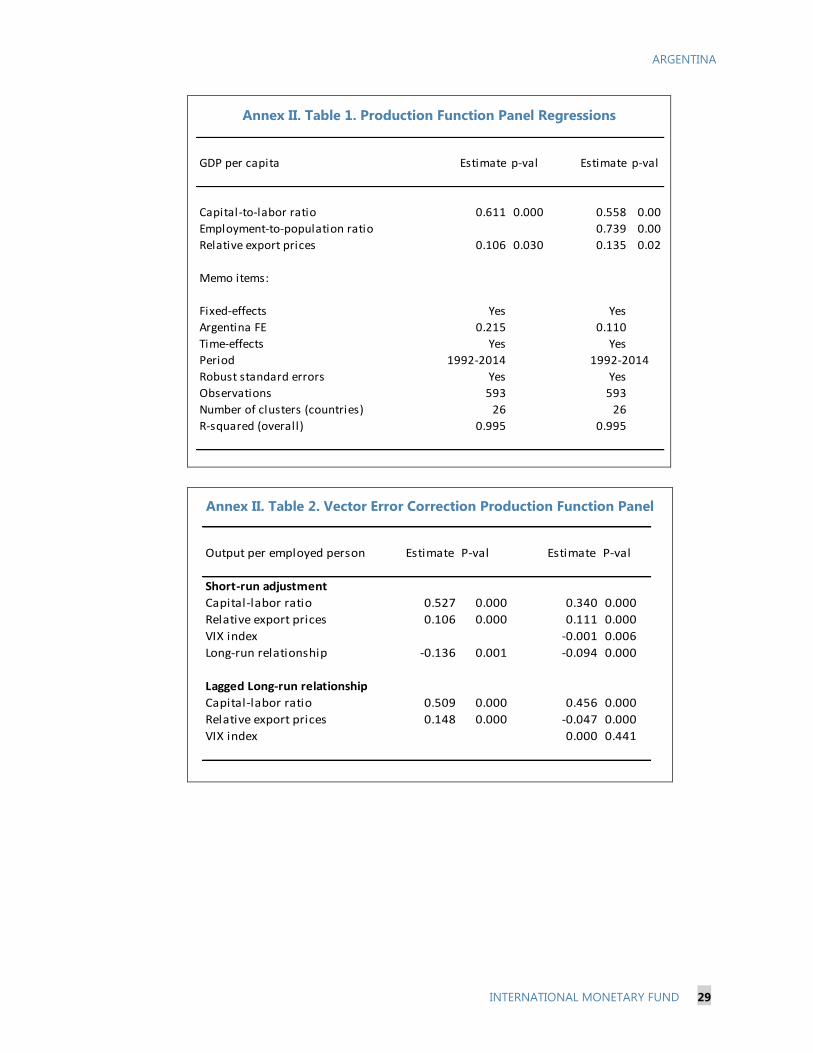
Annex II. Panel Production Function

Output per worker (or labor productivity) is a function of the capital stock and relative export prices.

This relationship holds as a panel for Argentina’s peer countries under a variety of measurements for

the capital stock and employment identified in the earlier sections. Estimates for the elasticity of

labor productivity to relative export prices varies between 10 and 14 percent across the different

measurements of the capital-to-labor ratio. In turn, the elasticity of the capital-to-labor ratio to labor

productivity ranges from 50 to 61 percent (Annex II. Table 1). Fixed effects for Argentina came out

negative under all specifications. The relationship between labor productivity, the capital-to-labor

ratio, and relative export prices also holds as a vector error correction form in a dynamic panel

specification. The long-term coefficient is 0.5 (Annex II Table 2).

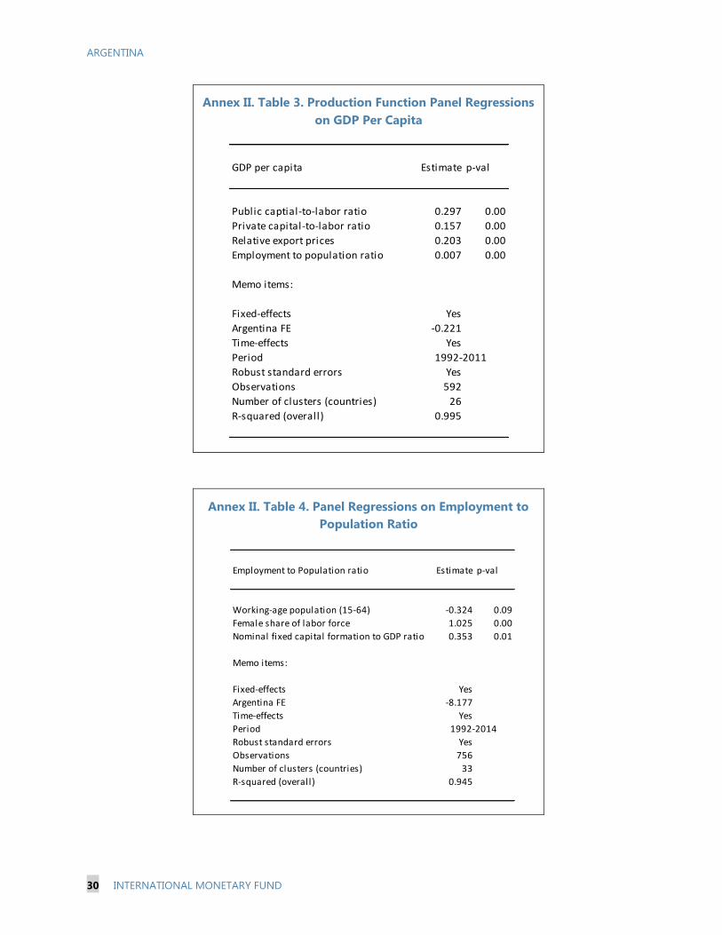
GDP per capita depends, by definition, on the same variables than output per worker and on the

share that the population that is employed. A panel regression under this specification delivers all

variables statistically significant and with the right signs (Annex II. Table 3). This prompts the

question of what determines the level of employment of the population. Although the share of the

population in working age (15–64) is a likely candidate, it turns out to be not significant under a

variety of specifications. Two important variables appear to play an important role. The first is the

female participation in the labor force, which is a slow moving (structural) characteristic of an

economy. The second is related to the business cycle fluctuations of an economy, and could be

proxied by the investment rate (Annex II. Table 4).

ARGENTINA


Annex II. Table 1. Production Function Panel Regressions

Annex II. Table 2. Vector Error Correction Production Function Panel

GDP per capita Estimate p-val Estimate p-val

Capital-to-labor ratio 0.611 0.000 0.558 0.00

Employment-to-population ratio 0.739 0.00

Relative export prices 0.106 0.030 0.135 0.02

Memo items:

Fixed-effects Yes Yes

Argentina FE 0.215 0.110

Time-effects Yes Yes

Period 1992-2014 1992-2014

Robust standard errors Yes Yes

Observations 593 593

Number of clusters (countries) 26 26

R-squared (overall) 0.995 0.995

Output per employed person Estimate P-val Estimate P-val

Short-run adjustment

Capital-labor ratio 0.527 0.000 0.340 0.000

Relative export prices 0.106 0.000 0.111 0.000

VIX index -0.001 0.006

Long-run relationship -0.136 0.001 -0.094 0.000

Lagged Long-run relationship

Capital-labor ratio 0.509 0.000 0.456 0.000

Relative export prices 0.148 0.000 -0.047 0.000

VIX index 0.000 0.441

ARGENTINA


Annex II. Table 3. Production Function Panel Regressions

on GDP Per Capita

Annex II. Table 4. Panel Regressions on Employment to

Population Ratio

GDP per capita Estimate p-val

Public captial-to-labor ratio 0.297 0.00

Private capital-to-labor ratio 0.157 0.00

Relative export prices 0.203 0.00

Employment to population ratio 0.007 0.00

Memo items:

Fixed-effects Yes

Argentina FE -0.221

Time-effects Yes

Period 1992-2011

Robust standard errors Yes

Observations 592

Number of clusters (countries) 26

R-squared (overall) 0.995

Employment to Population ratio Estimate p-val

Working-age population (15-64) -0.324 0.09

Female share of labor force 1.025 0.00

Nominal fixed capital formation to GDP ratio 0.353 0.01

Memo items:

Fixed-effects Yes

Argentina FE -8.177

Time-effects Yes

Period 1992-2014

Robust standard errors Yes

Observations 756

Number of clusters (countries) 33

R-squared (overall) 0.945

ARGENTINA


Annex III. Panel Charts for Selected Investment Surge Episodes

Argentina 2004–08

Argentina 2004-2008

10

12

14

16

18

20

22

24

26

28

30

-2 -1 0 1 2 3 4 5

Argentina

0.25-0.75 quartiles

0

1

2

3

4

5

6

7

8

9

-2 -1 0 1 2 3 4 5


-6

-5

-4

-3

-2

-1

0

1

2

3

4

-2 -1 0 1 2 3 4 5


15

17

19

21

23

25

27

29

-2 -1 0 1 2 3 4 5


2.5

3.0

3.5

4.0

4.5

5.0

-2 -1 0 1 2 3 4 510

12

14

16

18

20

22

24

26

28

30

-2 -1 0 1 2 3 4 5


50

60

70

80

90

100

110

120

130

-2 -1 0 1 2 3 4 5

0.0

0.5

1.0

1.5

2.0

2.5

3.0

3.5

4.0

-2 -1 0 1 2 3 4 5

years


ARGENTINA


Australia 1986–90

Australia: 1986-1990

15

17

19

21

23

25

27

29

-2 -1 0 1 2 3 4 5

Australia

0.25-0.75 quartiles

2

3

4

5

6

7

8

9

-2 -1 0 1 2 3 4 5


-6

-5

-4

-3

-2

-1

0

1

2

-2 -1 0 1 2 3 4 5


15

17

19

21

23

25

27

29

-2 -1 0 1 2 3 4 5


2.5

3.0

3.5

4.0

4.5

5.0

-2 -1 0 1 2 3 4 5

10

12

14

16

18

20

22

24

26

28

30

-2 -1 0 1 2 3 4 5

years


70

80

90

100

110

120

130

-2 -1 0 1 2 3 4 50.0

0.5

1.0

1.5

2.0

2.5

3.0

3.5

4.0

-2 -1 0 1 2 3 4 5


ARGENTINA


Mexico: 2004–09

Mexico: 2004-2009

15

17

19

21

23

25

27

29

-2 -1 0 1 2 3 4 5

Mexico

0.25-0.75 quartiles

2

3

4

5

6

7

8

9

-2 -1 0 1 2 3 4 5


-6

-5

-4

-3

-2

-1

0

1

2

-2 -1 0 1 2 3 4 5


15

17

19

21

23

25

27

29

-2 -1 0 1 2 3 4 5


2.5

3.0

3.5

4.0

4.5

5.0

-2 -1 0 1 2 3 4 510

12

14

16

18

20

22

24

26

28

30

-2 -1 0 1 2 3 4 5


70

80

90

100

110

120

130

-2 -1 0 1 2 3 4 50.0

0.5

1.0

1.5

2.0

2.5

3.0

3.5

4.0

-2 -1 0 1 2 3 4 5

years


ARGENTINA


New Zealand: 2001–05

New Zealand 2001-2005

15

17

19

21

23

25

27

29

-2 -1 0 1 2 3 4 5

New Zealand

0.25-0.75 quartiles2

3

4

5

6

7

8

9

-2 -1 0 1 2 3 4 5


-6

-4

-2

0

2

4

6

-2 -1 0 1 2 3 4 5


15

17

19

21

23

25

27

29

-2 -1 0 1 2 3 4 5


2.5

3.0

3.5

4.0

4.5

5.0

-2 -1 0 1 2 3 4 510

12

14

16

18

20

22

24

26

28

30

-2 -1 0 1 2 3 4 5


70

80

90

100

110

120

130

-2 -1 0 1 2 3 4 5

-6

-4

-2

0

2

4

6

-2 -1 0 1 2 3 4 5

years


ARGENTINA


Peru: 2005–10

Peru: 2005-10

15

17

19

21

23

25

27

29

-2 -1 0 1 2 3 4 5

Peru

0.25-0.75 quartiles2

3

4

5

6

7

8

9

-2 -1 0 1 2 3 4 5


-6

-5

-4

-3

-2

-1

0

1

2

3

4

-2 -1 0 1 2 3 4 5


15

17

19

21

23

25

27

29

-2 -1 0 1 2 3 4 5


2.5

3.0

3.5

4.0

4.5

5.0

-2 -1 0 1 2 3 4 510

12

14

16

18

20

22

24

26

28

30

-2 -1 0 1 2 3 4 5


70

80

90

100

110

120

130

-2 -1 0 1 2 3 4 50

1

2

3

4

5

6

-2 -1 0 1 2 3 4 5

years


ARGENTINA


Turkey: 2004–07

Turkey: 2004-2007

15

17

19

21

23

25

27

29

-2 -1 0 1 2 3 4 5

Turkey

0.25-0.75 quartiles

0

1

2

3

4

5

6

7

8

9

-2 -1 0 1 2 3 4 5


-16

-14

-12

-10

-8

-6

-4

-2

0

2

-2 -1 0 1 2 3 4 5


15

17

19

21

23

25

27

29

-2 -1 0 1 2 3 4 5


2.5

3.0

3.5

4.0

4.5

5.0

-2 -1 0 1 2 3 4 510

12

14

16

18

20

22

24

26

28

30

-2 -1 0 1 2 3 4 5


70

80

90

100

110

120

130

-2 -1 0 1 2 3 4 5

0.0

0.5

1.0

1.5

2.0

2.5

3.0

3.5

4.0

-2 -1 0 1 2 3 4 5

years


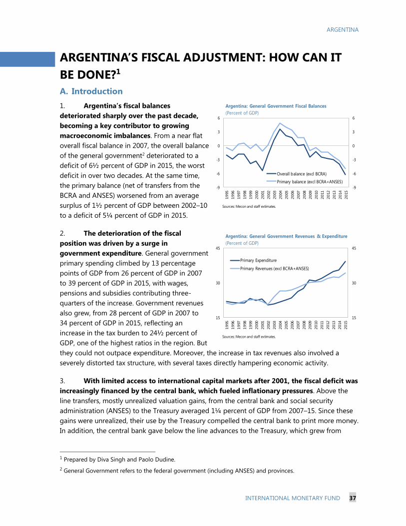
ARGENTINA


ARGENTINA’S FISCAL ADJUSTMENT: HOW CAN IT

BE DONE?1

A. Introduction

1. Argentina’s fiscal balances

deteriorated sharply over the past decade,

becoming a key contributor to growing

macroeconomic imbalances. From a near flat

overall fiscal balance in 2007, the overall balance

of the general government2 deteriorated to a

deficit of 6½ percent of GDP in 2015, the worst

deficit in over two decades. At the same time,

the primary balance (net of transfers from the

BCRA and ANSES) worsened from an average

surplus of 1½ percent of GDP between 2002–10

to a deficit of 5¼ percent of GDP in 2015.

2. The deterioration of the fiscal

position was driven by a surge in

government expenditure. General government

primary spending climbed by 13 percentage

points of GDP from 26 percent of GDP in 2007

to 39 percent of GDP in 2015, with wages,

pensions and subsidies contributing three-

quarters of the increase. Government revenues

also grew, from 28 percent of GDP in 2007 to

34 percent of GDP in 2015, reflecting an

increase in the tax burden to 24½ percent of

GDP, one of the highest ratios in the region. But

they could not outpace expenditure. Moreover, the increase in tax revenues also involved a

severely distorted tax structure, with several taxes directly hampering economic activity.

3. With limited access to international capital markets after 2001, the fiscal deficit was

increasingly financed by the central bank, which fueled inflationary pressures. Above the

line transfers, mostly unrealized valuation gains, from the central bank and social security

administration (ANSES) to the Treasury averaged 1¼ percent of GDP from 2007–15. Since these

gains were unrealized, their use by the Treasury compelled the central bank to print more money.

In addition, the central bank gave below the line advances to the Treasury, which grew from

1 Prepared by Diva Singh and Paolo Dudine.

2 General Government refers to the federal government (including ANSES) and provinces.

-9

-6

-3

0

3

6

-9

-6

-3

0

3

6

1995

1996

1997

1998

1999

2000

2001

2002

2003

2004

2005

2006

2007

2008

2009

2010

2011

2012

2013

2014

2015

Overall balance (excl BCRA)

Primary balance (excl BCRA+ANSES)

Argentina: General Government Fiscal Balances

(Percent of GDP)

Sources: Mecon and staff extimates.

15

30

45

15

30

45

1995

1996

1997

1998

1999

2000

2001

2002

2003

2004

2005

2006

2007

2008

2009

2010

2011

2012

2013

2014

2015

Primary Expenditure

Primary Revenues (excl BCRA+ANSES)

Argentina: General Government Revenues & Expenditure

(Percent of GDP)

Sources: Mecon and staff extimates.

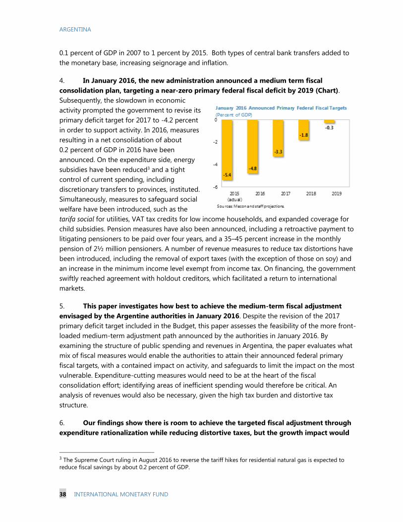
ARGENTINA


0.1 percent of GDP in 2007 to 1 percent by 2015. Both types of central bank transfers added to

the monetary base, increasing seignorage and inflation.

4. In January 2016, the new administration announced a medium term fiscal

consolidation plan, targeting a near-zero primary federal fiscal deficit by 2019 (Chart).

Subsequently, the slowdown in economic

activity prompted the government to revise its

primary deficit target for 2017 to -4.2 percent

in order to support activity. In 2016, measures

resulting in a net consolidation of about

0.2 percent of GDP in 2016 have been

announced. On the expenditure side, energy

subsidies have been reduced3 and a tight

control of current spending, including

discretionary transfers to provinces, instituted.

Simultaneously, measures to safeguard social

welfare have been introduced, such as the

tarifa social for utilities, VAT tax credits for low income households, and expanded coverage for

child subsidies. Pension measures have also been announced, including a retroactive payment to

litigating pensioners to be paid over four years, and a 35–45 percent increase in the monthly

pension of 2½ million pensioners. A number of revenue measures to reduce tax distortions have

been introduced, including the removal of export taxes (with the exception of those on soy) and

an increase in the minimum income level exempt from income tax. On financing, the government

swiftly reached agreement with holdout creditors, which facilitated a return to international

markets.

5. This paper investigates how best to achieve the medium-term fiscal adjustment

envisaged by the Argentine authorities in January 2016. Despite the revision of the 2017

primary deficit target included in the Budget, this paper assesses the feasibility of the more front-

loaded medium-term adjustment path announced by the authorities in January 2016. By

examining the structure of public spending and revenues in Argentina, the paper evaluates what

mix of fiscal measures would enable the authorities to attain their announced federal primary

fiscal targets, with a contained impact on activity, and safeguards to limit the impact on the most

vulnerable. Expenditure-cutting measures would need to be at the heart of the fiscal

consolidation effort; identifying areas of inefficient spending would therefore be critical. An

analysis of revenues would also be necessary, given the high tax burden and distortive tax

structure.

6. Our findings show there is room to achieve the targeted fiscal adjustment through

expenditure rationalization while reducing distortive taxes, but the growth impact would

3 The Supreme Court ruling in August 2016 to reverse the tariff hikes for residential natural gas is expected to

reduce fiscal savings by about 0.2 percent of GDP.

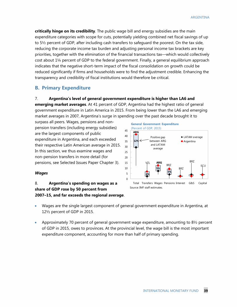
ARGENTINA


critically hinge on its credibility. The public wage bill and energy subsidies are the main

expenditure categories with scope for cuts, potentially yielding combined net fiscal savings of up

to 5½ percent of GDP, after including cash transfers to safeguard the poorest. On the tax side,

reducing the corporate income tax burden and adjusting personal income tax brackets are key

priorities, together with the elimination of the financial transactions tax—which would collectively

cost about 1¼ percent of GDP to the federal government. Finally, a general equilibrium approach

indicates that the negative short-term impact of the fiscal consolidation on growth could be

reduced significantly if firms and households were to find the adjustment credible. Enhancing the

transparency and credibility of fiscal institutions would therefore be critical.

B. Primary Expenditure

7. Argentina’s level of general government expenditure is higher than LA6 and

emerging market averages. At 41 percent of GDP, Argentina had the highest ratio of general

government expenditure in Latin America in 2015. From being lower than the LA6 and emerging

market averages in 2007, Argentina’s surge in spending over the past decade brought it to

surpass all peers. Wages, pensions and non-

pension transfers (including energy subsidies)

are the largest components of public

expenditure in Argentina, and each exceeded

their respective Latin American average in 2015.

In this section, we thus examine wages and

non-pension transfers in more detail (for

pensions, see Selected Issues Paper Chapter 3).

Wages

8. Argentina’s spending on wages as a

share of GDP rose by 50 percent from

2007–15, and far exceeds the regional average.

Wages are the single largest component of general government expenditure in Argentina, at

12½ percent of GDP in 2015.

Approximately 70 percent of general government wage expenditure, amounting to 8½ percent

of GDP in 2015, owes to provinces. At the provincial level, the wage bill is the most important

expenditure component, accounting for more than half of primary spending.

ARG

VZL ARGBRZ

BRZ

BRZ

ECU

0

5

10

15

20

25

30

35

40

45

Total Transfers Wages Pensions Interest G&S Capital

LATAM average

Argentina

Positive gap

between ARG

and LATAM

average

4%5%

5%

12%

General Government Expenditure

(Percent of GDP, 2015)

Source: IMF staff estimates.

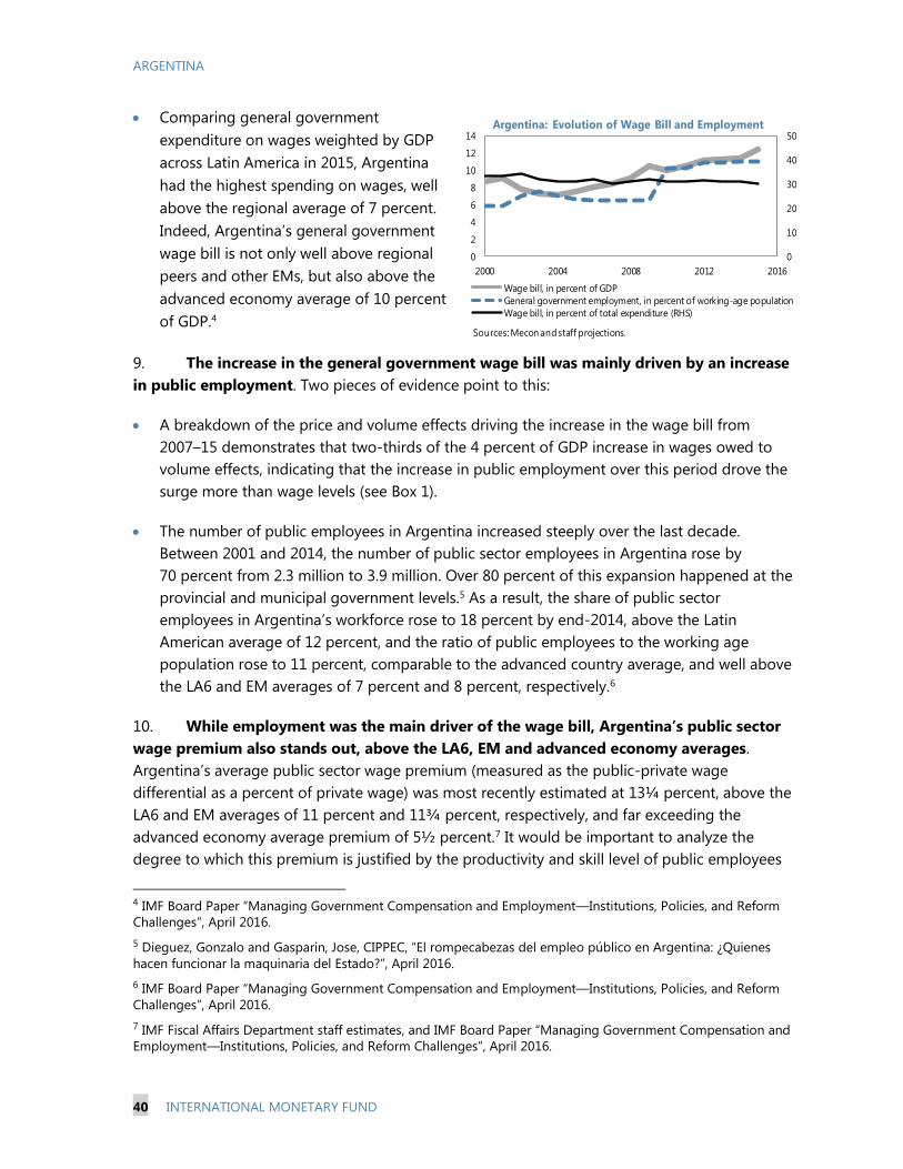
ARGENTINA


Comparing general government

expenditure on wages weighted by GDP

across Latin America in 2015, Argentina

had the highest spending on wages, well

above the regional average of 7 percent.

Indeed, Argentina’s general government

wage bill is not only well above regional

peers and other EMs, but also above the

advanced economy average of 10 percent

of GDP.4

9. The increase in the general government wage bill was mainly driven by an increase

in public employment. Two pieces of evidence point to this:

A breakdown of the price and volume effects driving the increase in the wage bill from

2007–15 demonstrates that two-thirds of the 4 percent of GDP increase in wages owed to

volume effects, indicating that the increase in public employment over this period drove the

surge more than wage levels (see Box 1).

The number of public employees in Argentina increased steeply over the last decade.

Between 2001 and 2014, the number of public sector employees in Argentina rose by

70 percent from 2.3 million to 3.9 million. Over 80 percent of this expansion happened at the

provincial and municipal government levels.5 As a result, the share of public sector

employees in Argentina’s workforce rose to 18 percent by end-2014, above the Latin

American average of 12 percent, and the ratio of public employees to the working age

population rose to 11 percent, comparable to the advanced country average, and well above

the LA6 and EM averages of 7 percent and 8 percent, respectively.6

10. While employment was the main driver of the wage bill, Argentina’s public sector

wage premium also stands out, above the LA6, EM and advanced economy averages.

Argentina’s average public sector wage premium (measured as the public-private wage

differential as a percent of private wage) was most recently estimated at 13¼ percent, above the

LA6 and EM averages of 11 percent and 11¾ percent, respectively, and far exceeding the

advanced economy average premium of 5½ percent.7 It would be important to analyze the

degree to which this premium is justified by the productivity and skill level of public employees

4 IMF Board Paper “Managing Government Compensation and Employment—Institutions, Policies, and Reform

Challenges”, April 2016.

5 Dieguez, Gonzalo and Gasparin, Jose, CIPPEC, “El rompecabezas del empleo público en Argentina: ¿Quienes

hacen funcionar la maquinaria del Estado?”, April 2016.

6 IMF Board Paper “Managing Government Compensation and Employment—Institutions, Policies, and Reform

Challenges”, April 2016.

7 IMF Fiscal Affairs Department staff estimates, and IMF Board Paper “Managing Government Compensation and

Employment—Institutions, Policies, and Reform Challenges”, April 2016.

0

10

20

30

40

50

0

2

4

6

8

10

12

14

2000 2004 2008 2012 2016

Wage bill, in percent of GDP

General government employment, in percent of working-age population

Wage bill, in percent of total expenditure (RHS)

Sources: Mecon and staff projections.

Argentina: Evolution of Wage Bill and Employment

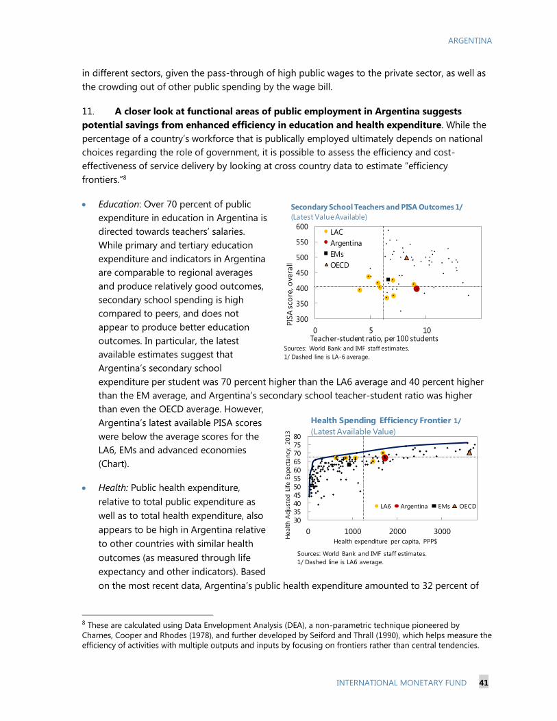
ARGENTINA


in different sectors, given the pass-through of high public wages to the private sector, as well as

the crowding out of other public spending by the wage bill.

11. A closer look at functional areas of public employment in Argentina suggests

potential savings from enhanced efficiency in education and health expenditure. While the

percentage of a country’s workforce that is publically employed ultimately depends on national

choices regarding the role of government, it is possible to assess the efficiency and cost-

effectiveness of service delivery by looking at cross country data to estimate “efficiency

frontiers.”8

Education: Over 70 percent of public

expenditure in education in Argentina is

directed towards teachers’ salaries.

While primary and tertiary education

expenditure and indicators in Argentina

are comparable to regional averages

and produce relatively good outcomes,

secondary school spending is high

compared to peers, and does not

appear to produce better education

outcomes. In particular, the latest

available estimates suggest that

Argentina’s secondary school

expenditure per student was 70 percent higher than the LA6 average and 40 percent higher

than the EM average, and Argentina’s secondary school teacher-student ratio was higher

than even the OECD average. However,

Argentina’s latest available PISA scores

were below the average scores for the

LA6, EMs and advanced economies

(Chart).

Health: Public health expenditure,

relative to total public expenditure as

well as to total health expenditure, also

appears to be high in Argentina relative

to other countries with similar health

outcomes (as measured through life

expectancy and other indicators). Based

on the most recent data, Argentina’s public health expenditure amounted to 32 percent of

8 These are calculated using Data Envelopment Analysis (DEA), a non-parametric technique pioneered by

Charnes, Cooper and Rhodes (1978), and further developed by Seiford and Thrall (1990), which helps measure the

efficiency of activities with multiple outputs and inputs by focusing on frontiers rather than central tendencies.

30

35

40

45

50

55

60

65

70

75

80

0 1000 2000 3000

He

alt

h A

dju

ste

d L

ife

Exp

ect

an

cy,

20

13

Health expenditure per capita, PPP$

LA6 Argentina EMs OECD

Health Spending Efficiency Frontier 1/

(Latest Available Value)

Sources: World Bank and IMF staff estimates.

1/ Dashed line is LA6 average.

300

350

400

450

500

550

600

0 5 10Teacher-student ratio, per 100 students

LAC

Argentina

EMs

OECD

Sources: World Bank and IMF staff estimates.

1/ Dashed line is LA-6 average.

Secondary School Teachers and PISA Outcomes 1/

(Latest Value Available)

PIS

Asco

re, o

vera

ll

ARGENTINA


total government expenditure, compared to 15 percent for the LA6 and OECD, and

12 percent for EMs. While this may simply indicate a policy choice to provide public

healthcare in Argentina, PPP-adjusted total health expenditure per capita in Argentina was

also significantly higher than the LA6 average, and almost double the EM average, while

health outcomes were largely in line with peers, below the efficiency frontier. Furthermore,

over two-thirds of public healthcare expenditure in Argentina is directed towards salaries

rather than capital investment in machinery, technology and health infrastructure. These

results suggest there could be room for enhancing efficiency by streamlining the public

healthcare workforce.

12. A combination of judiciously implemented employment and wage measures could

help reduce Argentina’s general government wage bill without negatively impacting

service delivery. The IMF Board Paper “Managing Government Compensation and

Employment—Institutions, Policies, and Reform Challenges” (April 2016) discusses lessons

learned from several country cases and presents a host of wage and employment measures that

have been effectively used to tackle wage bill pressures, many of which are relevant to Argentina.

For example, strengthening payroll management to track and control public employees and their

payroll, together with a census to identify ghost workers and double-dippers, could bring

important savings, without any negative impact on service delivery. In addition, while a first-best

approach involving a functional review of public sector ministries to merge units and streamline

employment would take time, the paper suggests an attrition-based reduction in public

employment, such as an elimination of certain retiring workers’ positions, could help raise

efficiency in the interim, without direct consequences to unemployment. On the wage-side of the

equation, an ad-hoc public wage adjustment, such as a temporary across the board nominal

wage freeze, could be warranted, especially given Argentina’s high public wage premium. So far,

the new administration has reportedly eliminated about 11,000 public sector jobs in 2016

through the downsizing of political employees and improperly hired personnel in various

ministries. Going forward, in September 2016, the administration unveiled a comprehensive plan

to increase efficiency in various ministries through voluntary retirement plans and the elimination

of redundant positions over the next two years.

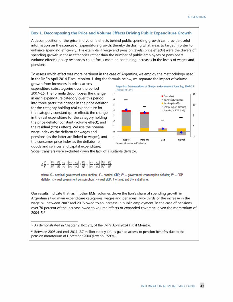
ARGENTINA


Box 1. Decomposing the Price and Volume Effects Driving Public Expenditure Growth

A decomposition of the price and volume effects behind public spending growth can provide useful

information on the sources of expenditure growth, thereby disclosing what areas to target in order to

enhance spending efficiency. For example, if wage and pension levels (price effects) were the drivers of

spending growth in these categories rather than the number of public employees or pensioners

(volume effects), policy responses could focus more on containing increases in the levels of wages and

pensions.

To assess which effect was more pertinent in the case of Argentina, we employ the methodology used

in the IMF’s April 2014 Fiscal Monitor. Using the formula below, we separate the impact of volume

growth from increases in prices across

expenditure subcategories over the period

2007–15. The formula decomposes the change

in each expenditure category over this period

into three parts: the change in the price deflator

for the category holding real expenditure for

that category constant (price effect); the change

in the real expenditure for the category holding

the price deflator constant (volume effect); and

the residual (cross effect). We use the nominal

wage index as the deflator for wages and

pensions (as the latter are linked to wages), and

the consumer price index as the deflator for

goods and services and capital expenditure.

Social transfers were excluded given the lack of a suitable deflator.

Our results indicate that, as in other EMs, volumes drove the lion’s share of spending growth in

Argentina’s two main expenditure categories: wages and pensions. Two-thirds of the increase in the

wage bill between 2007 and 2015 owed to an increase in public employment. In the case of pensions,

over 70 percent of the increase owed to volume effects or expanded coverage, given the moratorium of

2004–5.2

_______________________________

1/ As demonstrated in Chapter 2, Box 2.1, of the IMF’s April 2014 Fiscal Monitor.

2/ Between 2005 and end-2011, 2.7 million elderly adults gained access to pension benefits due to the

pension moratorium of December 2004 (Law no. 25994).

-5

0

5

10

15

-1

0

1

2

3

4

5

6

7

Wages Pensions G&S Capital

Cross effect

Relative volume effect

Relative price effect

Change in govt spending

Spending in 2015 (RHS)

Argentina: Decomposition of Change in Government Spending, 2007-15

(Percent of GDP)

Sources: Mecon and staff estimates.

ARGENTINA


Energy subsidies

13. Energy subsidies have risen dramatically in Argentina over the past decade causing

social transfers to far exceed the regional average. At the general government level,

Argentina spent 6¾ percent of GDP on social transfers in 2015, against a regional average of

2¼ percent. Most of these transfers (6 percent of GDP) are at the federal level, and comprise

energy subsidies (4 percent of GDP). The increase in federal energy subsidies, from 1¼ percent of

GDP in 2007, happened as a result of the government’s policy to keep domestic energy tariffs

largely constant after 2002, in an attempt to prevent the pass-through of high international

energy prices to consumers. The policy hurt the domestic energy sector—as tariffs fell well

behind production costs and inflation. As investment in the energy sector declined due to the

unpropitious environment in the sector, there was a gradual rise in the share of imported energy.

Increased import dependency, in turn, hurt the fiscal accounts, particularly in light of the

significant depreciation of the nominal exchange rate over this period (between 2011 and 2014,

the average nominal exchange rate of the Argentine peso against the U.S. dollar depreciated

50 percent in foreign currency terms). Staff estimates for the impact of exchange rate

depreciation on energy subsidy expenditures, using simple OLS regressions, suggest an elasticity

of close to 1. Thus, the increasing share of energy imports coupled with currency depreciation

were a direct blow to the government’s energy subsidy bill. Indeed, staff estimates suggest the

peso depreciation since December 2015 would have increased the energy subsidy bill to about

5½ percent of GDP in 2016, assuming no policy changes.

14. Energy subsidies are poorly targeted. As in other countries, energy subsidies in

Argentina are largely regressive, with many poor segments of the population lacking access to

the subsidized products. In particular, a 2015 study by CIPPEC estimated that the poorest

20 percent of households only received 12 percent of natural gas subsidies, and 18 percent of

electricity subsidies, while the richest two deciles received 39 percent and 21 percent,

respectively. The statistics for public transport are no better, with the poorest 20 percent

receiving 11 percent of bus subsidies and 3 percent of train/tram subsidies, compared to

21 percent and 29 percent, respectively, for the top two income deciles. This suggests that public

resources that are currently devoted to subsidize households that can afford to pay in full could

be redirected towards well-targeted social programs and at the same time achieve fiscal savings.

Given the small share of total energy subsidies received by low-income groups, staff estimates

suggest that fully compensating the bottom 4 income deciles for a complete elimination of

subsidies would bear a fiscal cost of only ½ percent of GDP (see Box 2). This compares to the

gross fiscal gains from eliminating energy subsidies of 5½ percent of GDP. Thus, the net fiscal

gains from subsidy reform, after fully compensating the bottom 40 percent of households, could

potentially amount to as much as 5 percent of GDP.

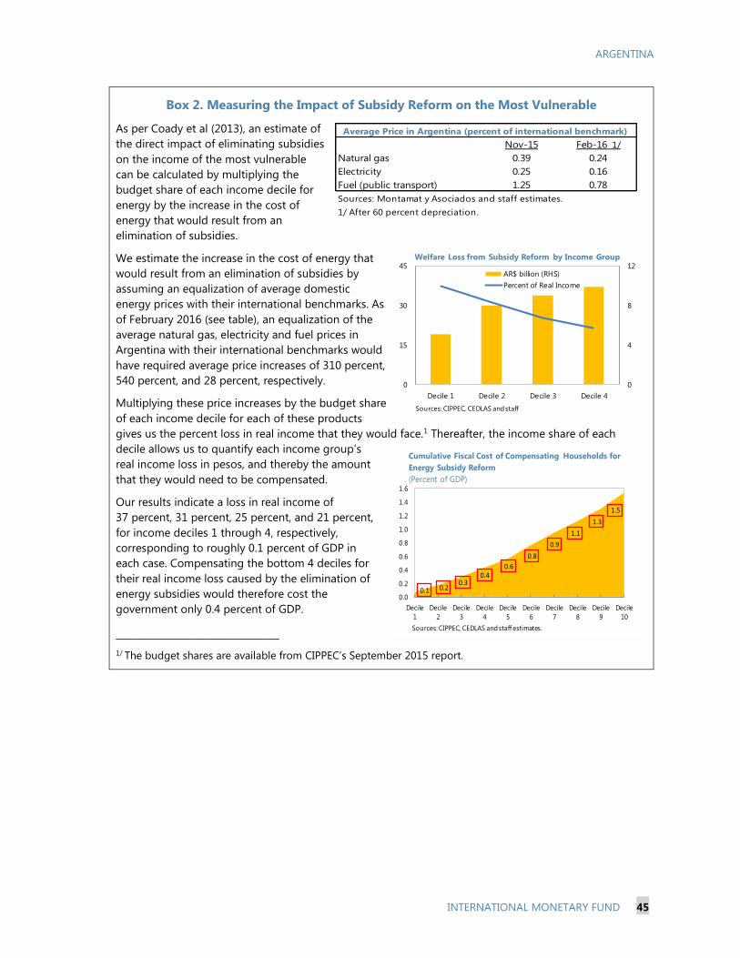
ARGENTINA


Box 2. Measuring the Impact of Subsidy Reform on the Most Vulnerable

As per Coady et al (2013), an estimate of

the direct impact of eliminating subsidies

on the income of the most vulnerable

can be calculated by multiplying the

budget share of each income decile for

energy by the increase in the cost of

energy that would result from an

elimination of subsidies.

We estimate the increase in the cost of energy that

would result from an elimination of subsidies by

assuming an equalization of average domestic

energy prices with their international benchmarks. As

of February 2016 (see table), an equalization of the

average natural gas, electricity and fuel prices in

Argentina with their international benchmarks would

have required average price increases of 310 percent,

540 percent, and 28 percent, respectively.

Multiplying these price increases by the budget share

of each income decile for each of these products

gives us the percent loss in real income that they would face.1 Thereafter, the income share of each

decile allows us to quantify each income group’s

real income loss in pesos, and thereby the amount

that they would need to be compensated.

Our results indicate a loss in real income of

37 percent, 31 percent, 25 percent, and 21 percent,

for income deciles 1 through 4, respectively,

corresponding to roughly 0.1 percent of GDP in

each case. Compensating the bottom 4 deciles for

their real income loss caused by the elimination of

energy subsidies would therefore cost the

government only 0.4 percent of GDP.

_______________________________

1/ The budget shares are available from CIPPEC’s September 2015 report.

0.1 0.20.3

0.40.6

0.8

0.9

1.1

1.3

1.5

0.0

0.2

0.4

0.6

0.8

1.0

1.2

1.4

1.6

Decile

1

Decile

2

Decile

3

Decile

4

Decile

5

Decile

6

Decile

7

Decile

8

Decile

9

Decile

10

Cumulative Fiscal Cost of Compensating Households for

Energy Subsidy Reform

(Percent of GDP)

Sources: CIPPEC, CEDLAS and staff estimates.

0

4

8

12

0

15

30

45

Decile 1 Decile 2 Decile 3 Decile 4

AR$ billion (RHS)

Percent of Real Income

Welfare Loss from Subsidy Reform by Income Group

Sources: CIPPEC, CEDLAS and staff

Nov-15 Feb-16 1/

Natural gas 0.39 0.24

Electricity 0.25 0.16

Fuel (public transport) 1.25 0.78

Sources: Montamat y Asociados and staff estimates.

1/ After 60 percent depreciation.

Average Price in Argentina (percent of international benchmark)

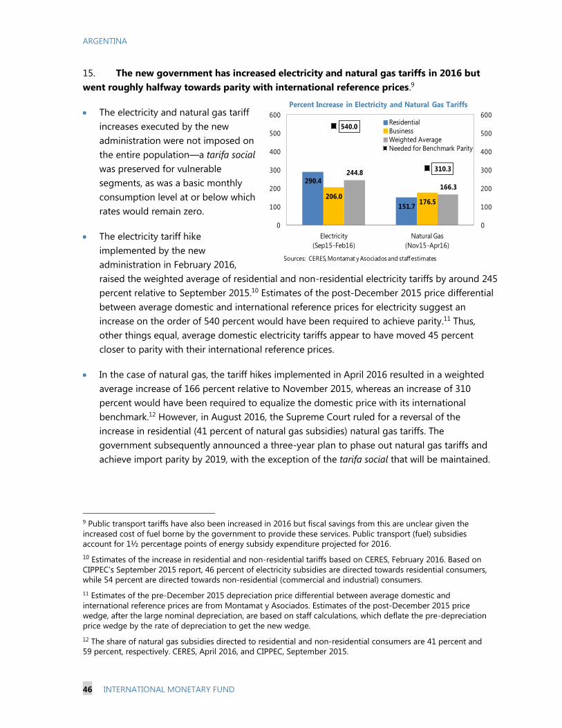
ARGENTINA


15. The new government has increased electricity and natural gas tariffs in 2016 but

went roughly halfway towards parity with international reference prices.9

The electricity and natural gas tariff

increases executed by the new

administration were not imposed on

the entire population—a tarifa social

was preserved for vulnerable

segments, as was a basic monthly

consumption level at or below which

rates would remain zero.

The electricity tariff hike

implemented by the new

administration in February 2016,

raised the weighted average of residential and non-residential electricity tariffs by around 245

percent relative to September 2015.10 Estimates of the post-December 2015 price differential

between average domestic and international reference prices for electricity suggest an

increase on the order of 540 percent would have been required to achieve parity.11 Thus,

other things equal, average domestic electricity tariffs appear to have moved 45 percent

closer to parity with their international reference prices.

In the case of natural gas, the tariff hikes implemented in April 2016 resulted in a weighted

average increase of 166 percent relative to November 2015, whereas an increase of 310

percent would have been required to equalize the domestic price with its international

benchmark.12 However, in August 2016, the Supreme Court ruled for a reversal of the

increase in residential (41 percent of natural gas subsidies) natural gas tariffs. The

government subsequently announced a three-year plan to phase out natural gas tariffs and

achieve import parity by 2019, with the exception of the tarifa social that will be maintained.

9 Public transport tariffs have also been increased in 2016 but fiscal savings from this are unclear given the

increased cost of fuel borne by the government to provide these services. Public transport (fuel) subsidies

account for 1½ percentage points of energy subsidy expenditure projected for 2016.

10 Estimates of the increase in residential and non-residential tariffs based on CERES, February 2016. Based on

CIPPEC’s September 2015 report, 46 percent of electricity subsidies are directed towards residential consumers,

while 54 percent are directed towards non-residential (commercial and industrial) consumers.

11 Estimates of the pre-December 2015 depreciation price differential between average domestic and

international reference prices are from Montamat y Asociados. Estimates of the post-December 2015 price

wedge, after the large nominal depreciation, are based on staff calculations, which deflate the pre-depreciation

price wedge by the rate of depreciation to get the new wedge.

12 The share of natural gas subsidies directed to residential and non-residential consumers are 41 percent and

59 percent, respectively. CERES, April 2016, and CIPPEC, September 2015.

290.4

151.7

206.0176.5

244.8

166.3

540.0

310.3

0

100

200

300

400

500

600

0

100

200

300

400

500

600

Electricity

(Sep15-Feb16)

Natural Gas

(Nov15-Apr16)

Residential

Business

Weighted Average

Needed for Benchmark Parity

Sources: CERES, Montamat y Asociados and staff estimates

Percent Increase in Electricity and Natural Gas Tariffs

ARGENTINA


Since electricity and natural gas account for 75 percent of the government’s energy subsidy

expenditure, the executed increase in their tariffs, even after the Supreme Court ruling on

residential natural gas tariffs, is estimated to reduce the fiscal cost of subsidies by about

1¾ percent of GDP in 2016.

16. Full elimination of remaining electricity and natural gas subsidies would yield

additional gross fiscal savings of about 2¼ percent of GDP. Of the 5½ percent of GDP in

energy subsidies estimated for 2016, 4 percentage points are accounted for by electricity and

natural gas subsidies. Given the 1¾ percent of GDP reduction in these subsidies expected

through the tariff hikes already implemented, another 2¼ percent of GDP in gross fiscal savings

could be garnered from a full elimination of these subsidies through further tariff hikes of

55 percent for electricity and 46 percent for natural gas, to close the gap with international

reference prices. Even after compensating the bottom 4 income deciles for their loss in real

income arising from this, the government would see net fiscal savings of 1¾ percent of GDP.

17. In order to achieve and maintain full cost recovery on remaining energy subsidies,

the adoption of a rule-based automatic price adjustment mechanism for setting energy

tariffs is strongly recommended. As international experience shows, adoption of an automatic

price adjustment formula to set energy tariffs reduces the uncertainty on the future cost of

energy, which is likely to be an important disincentive for investment, and also reduces the level

and volatility of the fiscal cost of energy pricing policy. Implementing such a mechanism would

require the establishment of a clear pricing structure for each energy product, linking retail prices

of the product with international prices, based on costs, margins, taxes, as well as an agreed

mechanism for handling import price volatility (see Coady et al, 2012).

C. Tax Revenues

18. Argentina’s tax burden increased dramatically in the past ten years and is one of the

highest in the region and among emerging markets. The ratio of tax revenue to GDP started to

increase in 2001, following the introduction of the highly distortive financial transaction tax and

export taxes. During 2006–15 overall general government tax revenue increased sharply, by over

7 percentage points of GDP reaching 32 percent of GDP, 10 percentage points above the regional

average and only about 4 points below the OECD average.13 Most of the increase came from a

pickup in the VAT, a jump in social security contributions (mostly explained by the reabsorption of

private pension schemes into the public sector), and, since 2011, a pickup in the personal income

tax (PIT), mainly as the lack of indexation of income brackets since 2001 meant that inflation pushed

more and more tax payers into brackets with higher marginal rates, and the lack of indexation of the

non-taxable income and other deductions meant that the effective tax rates increased.

13 It includes social security contributions.

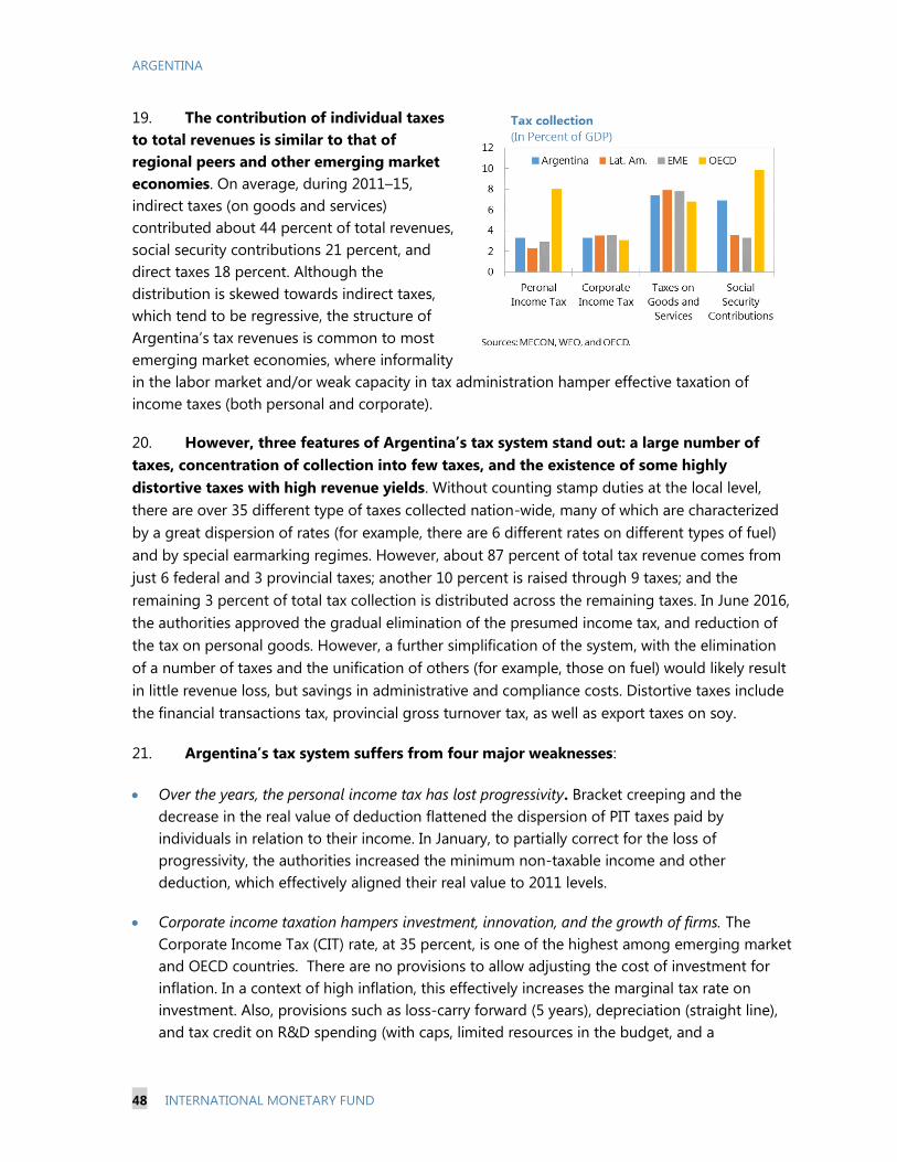
ARGENTINA


19. The contribution of individual taxes

to total revenues is similar to that of

regional peers and other emerging market

economies. On average, during 2011–15,

indirect taxes (on goods and services)

contributed about 44 percent of total revenues,

social security contributions 21 percent, and

direct taxes 18 percent. Although the

distribution is skewed towards indirect taxes,

which tend to be regressive, the structure of

Argentina’s tax revenues is common to most

emerging market economies, where informality

in the labor market and/or weak capacity in tax administration hamper effective taxation of

income taxes (both personal and corporate).

20. However, three features of Argentina’s tax system stand out: a large number of

taxes, concentration of collection into few taxes, and the existence of some highly

distortive taxes with high revenue yields. Without counting stamp duties at the local level,

there are over 35 different type of taxes collected nation-wide, many of which are characterized

by a great dispersion of rates (for example, there are 6 different rates on different types of fuel)

and by special earmarking regimes. However, about 87 percent of total tax revenue comes from

just 6 federal and 3 provincial taxes; another 10 percent is raised through 9 taxes; and the

remaining 3 percent of total tax collection is distributed across the remaining taxes. In June 2016,

the authorities approved the gradual elimination of the presumed income tax, and reduction of

the tax on personal goods. However, a further simplification of the system, with the elimination

of a number of taxes and the unification of others (for example, those on fuel) would likely result

in little revenue loss, but savings in administrative and compliance costs. Distortive taxes include

the financial transactions tax, provincial gross turnover tax, as well as export taxes on soy.

21. Argentina’s tax system suffers from four major weaknesses:

Over the years, the personal income tax has lost progressivity. Bracket creeping and the

decrease in the real value of deduction flattened the dispersion of PIT taxes paid by

individuals in relation to their income. In January, to partially correct for the loss of

progressivity, the authorities increased the minimum non-taxable income and other

deduction, which effectively aligned their real value to 2011 levels.

Corporate income taxation hampers investment, innovation, and the growth of firms. The

Corporate Income Tax (CIT) rate, at 35 percent, is one of the highest among emerging market

and OECD countries. There are no provisions to allow adjusting the cost of investment for

inflation. In a context of high inflation, this effectively increases the marginal tax rate on

investment. Also, provisions such as loss-carry forward (5 years), depreciation (straight line),

and tax credit on R&D spending (with caps, limited resources in the budget, and a

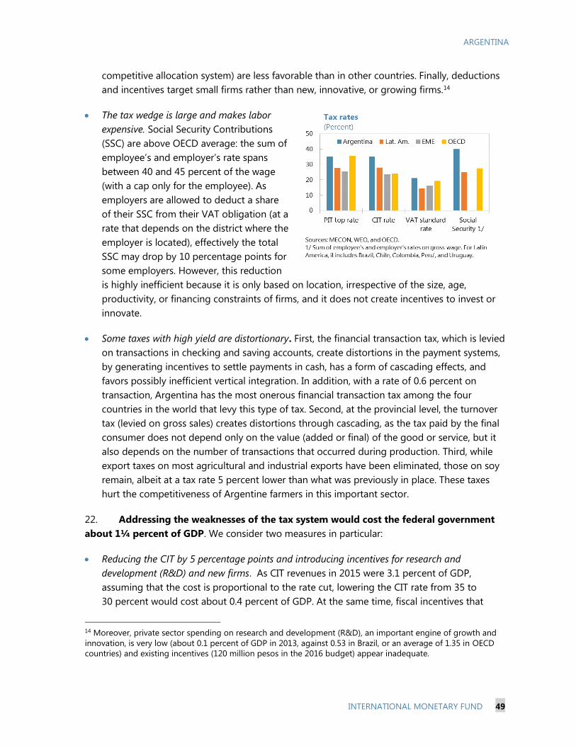
ARGENTINA


competitive allocation system) are less favorable than in other countries. Finally, deductions

and incentives target small firms rather than new, innovative, or growing firms.14

The tax wedge is large and makes labor

expensive. Social Security Contributions

(SSC) are above OECD average: the sum of

employee’s and employer’s rate spans

between 40 and 45 percent of the wage

(with a cap only for the employee). As

employers are allowed to deduct a share

of their SSC from their VAT obligation (at a

rate that depends on the district where the

employer is located), effectively the total

SSC may drop by 10 percentage points for

some employers. However, this reduction

is highly inefficient because it is only based on location, irrespective of the size, age,

productivity, or financing constraints of firms, and it does not create incentives to invest or

innovate.

Some taxes with high yield are distortionary. First, the financial transaction tax, which is levied

on transactions in checking and saving accounts, create distortions in the payment systems,

by generating incentives to settle payments in cash, has a form of cascading effects, and

favors possibly inefficient vertical integration. In addition, with a rate of 0.6 percent on

transaction, Argentina has the most onerous financial transaction tax among the four

countries in the world that levy this type of tax. Second, at the provincial level, the turnover

tax (levied on gross sales) creates distortions through cascading, as the tax paid by the final

consumer does not depend only on the value (added or final) of the good or service, but it

also depends on the number of transactions that occurred during production. Third, while

export taxes on most agricultural and industrial exports have been eliminated, those on soy

remain, albeit at a tax rate 5 percent lower than what was previously in place. These taxes

hurt the competitiveness of Argentine farmers in this important sector.

22. Addressing the weaknesses of the tax system would cost the federal government

about 1¼ percent of GDP. We consider two measures in particular:

Reducing the CIT by 5 percentage points and introducing incentives for research and

development (R&D) and new firms. As CIT revenues in 2015 were 3.1 percent of GDP,

assuming that the cost is proportional to the rate cut, lowering the CIT rate from 35 to

30 percent would cost about 0.4 percent of GDP. At the same time, fiscal incentives that

14 Moreover, private sector spending on research and development (R&D), an important engine of growth and

innovation, is very low (about 0.1 percent of GDP in 2013, against 0.53 in Brazil, or an average of 1.35 in OECD

countries) and existing incentives (120 million pesos in the 2016 budget) appear inadequate.

ARGENTINA


halve the private cost of R&D (which is estimated to be the efficient level of such incentives15)

would cost 0.1 percent of GDP.16 As the CIT is also shared with provinces, the revenue loss for

the federal budget would be slightly above 0.2 percent of GDP. The loss at the provincial

level from CIT reforms could partly be compensated by substituting the turnover tax for a

more efficient provincial tax on goods and services, or by increasing property taxes, which

are currently low by international standards.

Eliminating the financial transaction tax would imply a loss for the federal government of

1 percent of GDP, excluding the provincial share in this tax.17

D. Assessing the Economic Impact of Fiscal Consolidation

23. In this section, we assess the impact of fiscal consolidation packages on economic

activity in Argentina. The packages considered here deliver the adjustment in the federal

primary fiscal deficit announced in January 2016 (for a cumulative 4½ percent of GDP).

Leveraging on the review of Argentina’s expenditure in Section II, we contemplate adjustment

packages involving spending cuts in areas that lack efficiency, as well as measures to reduce the

tax burden and improve the tax system, by addressing some of the major weaknesses identified

in Section III.

24. To do so we use the Flexible System of Global Models (FSGM), one of the general

equilibrium models available at the IMF.18 The advantage of simulating the impact of fiscal

policy on growth using a general equilibrium model is that it allows us to examine the behavior

of the economy at large, by analyzing the interaction of various microeconomic decisions (IMF,

2014). Needless to say, the results of the analysis are very sensitive to the model’s parameters

and specific modeling assumptions; in particular:

Whether the fiscal consolidation package is credible. If the fiscal authorities are credible and

agents fully anticipate that the fiscal consolidation will be implemented as announced, this

triggers agents to adjust their investment and consumption decisions, bringing forward the

long-run benefit of the fiscal adjustment. For this reason, the short-term output costs of the

consolidation are diminished.

The share of liquidity constrained agents in the economy. The greater the share of households

that lack access to financial markets and savings instruments, and thus consume all their

income in each period, the stronger the impact of fiscal policy.

25. For the purposes of our simulations, we assume partial credibility and a 60 percent

share of liquidity constrained households. It would be unrealistic to assume complete

15 IMF, 2016, “Acting Now, Acting Together”, Fiscal Monitor April 2016.

16 It assumes an elasticity of 1 of R&D spending to its cost.

17 This is the amount collected in 2015. Going forward, we assume an elasticity of 1 of this tax to GDP.

18 A description of the model can be found in Annex II.

ARGENTINA


credibility for the new administration, given the track record of previous administrations and the

history of expansionary fiscal policy in Argentina. Nonetheless, it would also be unreasonable to

assume no credibility, given the multitude of measures already implemented by the new

government. We therefore simulate our models under the assumption of partial (or growing)

credibility, with agents only believing that the change in policy will be permanent once it has

been in place for two years. With respect to liquidity constrained households, we assume a

60 percent share for Argentina, in line with the average share for EMs.

26. First, we simulate a fiscal consolidation package that only includes expenditure

measures. This package (Table: Adjustment Scenario 1) assumes that the federal government

achieves a 1½ percent of GDP consolidation per year from 2017–19 to meet its primary targets

through expenditure measures that build on the analysis in Section II. In particular:

A reduction in the wage bill of 2 percent of GDP.19

A reduction in energy subsidies of 3½ percent of GDP.

A ½ percent of GDP increase in cash transfers to households, which, as explained in Section

II, compensates the bottom 40 percent of the population for the subsidy cuts.

A ½ percent of GDP increase in capital expenditure (which, at 3½ percent of GDP in 2015

was below the regional average of 5 percent).

27. Next, we simulate a fiscal adjustment scenario that also adds tax cuts. This scenario

assumes the same overall fiscal consolidation as the previous, but adds tax cuts in addition to

spending measures, to correct some of the distortions highlighted in Section III (Table:

Adjustment Scenario 2). In particular, the scenario incorporates:

A 2¾ percent of GDP reduction in the wage bill.

A 3½ percent of GDP reduction in energy subsidies,

A ½ percent of GDP increase in cash transfers to the bottom 4 deciles to compensate them

for the subsidy cuts.

A ¼ percent of GDP increase in capital spending.

A 0.6 percent of GDP decrease in taxes on households’ income (through the financial

transactions tax).

19 As noted in Section II, the bulk of the wage bill is at the provincial level. Still, we assume that apart from

reducing the federal wage bill, the federal government reduces discretionary federal transfers to provinces, and

that provinces react by lowering their wage bill by the same amount.

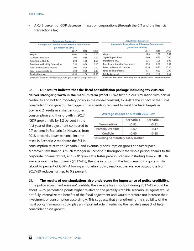
ARGENTINA


A 0.45 percent of GDP decrease in taxes on corporations (through the CIT and the financial

transactions tax)

28. Our results indicate that the fiscal consolidation package including tax cuts can

deliver stronger growth in the medium term (Panel 1). We first run our simulation with partial

credibility and holding monetary policy in the model constant, to isolate the impact of the fiscal

consolidation on growth. The bigger cut in spending required to meet the fiscal targets in

Scenario 2 results in a sharper drop in

consumption and thus growth in 2017

(GDP growth falls by 1.2 percent in the

first year of the adjustment compared to

0.7 percent in Scenario 1). However, from

2018 onwards, lower personal income

taxes in Scenario 2 moderate the fall in

consumption relative to Scenario 1 and eventually consumption grows at a faster pace.

Moreover, investment is much stronger in Scenario 2 throughout the whole period, thanks to the

corporate income tax cut, and GDP grows at a faster pace in Scenario 2 starting from 2018. On

average over the first 3 years (2017–19), the loss in output in the two scenarios is quite similar

(about ½ percent of GDP). Allowing a monetary policy reaction, the average output loss from

2017–19 reduces further, to 0.2 percent.

29. The results of our simulations also underscore the importance of policy credibility.

If the policy adjustment were not credible, the average loss in output during 2017–19 would be

about ¼–½ percentage points higher relative to the partially-credible scenario, as agents would

not fully internalize the benefits of the fiscal adjustment and would therefore not increase their

investment or consumption accordingly. This suggests that strengthening the credibility of the

fiscal policy framework could play an important role in reducing the negative impact of fiscal

consolidation on growth.

2017 2018 2019

Wages -1.00 -1.00 0.00

Capital Expenditure 0.00 0.50 0.00

Transfers to OLG 1/ -1.00 -1.00 -1.50

Transfers to Liquidity Constrained 0.50 0.00 0.00

Taxes on household income 0.00 0.00 0.00

Taxes on corporations 0.00 0.00 0.00

Total adjustment -1.50 -1.50 -1.50

1/ Assumes a reduction in electricity, natural gas and public transport subsidies.

Adjustment Scenario 1

(In Percent of GDP)

Changes in Expenditure and Revenue Components

2017 2018 2019

Wages -1.00 -1.00 -0.80

Capital Expenditure 0.00 0.25 0.00

Transfers to OLG -1.25 -1.25 -1.00

Transfers to Liquidity Constrained 0.50 0.00 0.00

Taxes on household income -0.10 -0.20 -0.30

Taxes on corporations -0.15 -0.30 0.00

Total adjustment -1.50 -1.50 -1.50

1/ Assumes a reduction in electricity, natural gas and public transport subsidies.

Changes in Expenditure and Revenue Components

(In Percent of GDP)

Adjustment Scenario 2

Average Impact on Growth 2017–19*

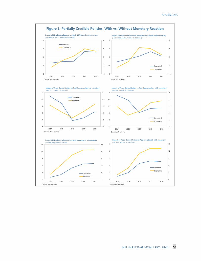
ARGENTINA


Figure 1. Partially Credible Policies, With vs. Without Monetary Reaction

-2

-1

0

1

2

-2

-1

0

1

2

2017 2018 2019 2020 2021

Scenario 1

Scenario 2

Source: staff estimates.

Impact of Fiscal Consolidation on Real GDP growth: no monetary

(percentage points, relative to baseline)

-2

-1

0

1

2

-2

-1

0

1

2

2017 2018 2019 2020 2021

Scenario 1

Scenario 2


Impact of Fiscal Consolidation on Real GDP growth: with monetary


-5

-4

-3

-2

-1

0

-5

-4

-3

-2

-1

0

2017 2018 2019 2020 2021

Scenario 1

Scenario 2

Source: staff estimates

Impact of Fiscal Consolidation on Real Consumption: no monetary

(percent, relative to baseline)

-5

-4

-3

-2

-1

0

-5

-4

-3

-2

-1

0

2017 2018 2019 2020 2021

Scenario 1

Scenario 2


Impact of Fiscal Consolidation on Real Consumption: with monetary


0

3

6

9

12

15

0

3

6

9

12

15

2017 2018 2019 2020 2021

Scenario 1

Scenario 2


Impact of Fiscal Consolidation on Real Investment: no monetary


0

3

6

9

12

15

0

3

6

9

12

15

2017 2018 2019 2020 2021

Scenario 1

Scenario 2


Impact of Fiscal Consolidation on Real Investment: with monetary


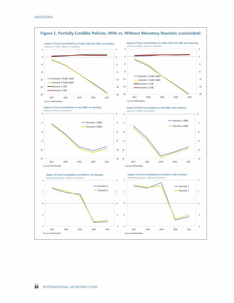
ARGENTINA


Figure 1. Partially Credible Policies, With vs. Without Monetary Reaction (concluded)

-20

-16

-12

-8

-4

0

4

-20

-16

-12

-8

-4

0

4

2017 2018 2019 2020 2021

Scenario 1 Public Debt


Scenario 1 CAB

Scenario 2 CAB


Impact of Fiscal Consolidation on Public Debt and CAB: no monetary

(percent of GDP, relative to baseline)

-15

-12

-9

-6

-3

0

-15

-12

-9

-6

-3

0

2017 2018 2019 2020 2021

Scenario 1 REER

Scenario 2 REER


Impact of Fiscal Consolidation on the REER: no monetary


-15

-12

-9

-6

-3

0

-15

-12

-9

-6

-3

0

2017 2018 2019 2020 2021

Scenario 1 REER

Scenario 2 REER


Impact of Fiscal Consolidation on the REER: with monetary


-2

-1

0

1

2

-2

-1

0

1

2

2017 2018 2019 2020 2021

Scenario 1

Scenario 2


Impact of Fiscal Consolidation on Inflation: no monetary


-2

-1

0

1

2

-2

-1

0

1

2

2017 2018 2019 2020 2021

Scenario 1

Scenario 2


Impact of Fiscal Consolidation on Inflation: with monetary


-20

-16

-12

-8

-4

0

4

-20

-16

-12

-8

-4

0

4

2017 2018 2019 2020 2021



Scenario 1 CAB

Scenario 2 CAB


Impact of Fiscal Consolidation on Public Debt and CAB: with monetary

(percent of GDP, relative to baseline)

ARGENTINA


References

Anderson, D., B. Hunt, M. Kortelainen, M. Kumhof, D. Laxton, D. Muir, S. Mursula, and S. Snudden.

(2013). “Getting to Know GIMF: The Simulation Properties of the Global Integrated Monetary

and Fiscal Model.” IMF Working Paper No. 13/55. International Monetary Fund.

Andrle, Michal, Patrick Blagrave, Pedro Espaillat, Keiko Honjo, Benjamin Hunt, Mika Kortelainen,

René Lalonde, Douglas Laxton, Eleonora Mavroeidi, Dirk Muir, and Susanna Mursula. 2015.

“The Flexible System of Global Models–FSGM.” Working Paper 15/64, International Monetary

Fund, Washington.

Blagrave, P., C. Godbout, J.D. Guenette and R. Lalonde. (2015). “G-MUSE: The Bank of Canada

Projection Model for the Global Economy.” Bank of Canada Technical Report, forthcoming.

Brayton, F., and P. Tinsley. (1996). “A Guide to FRB/US: A Macroeconomic Model of the United

States.” Board of Governors of the Federal Reserves System Finance and Economics

Discussion Series 96–42. Board of Governors of the Federal Reserve System

Coady et al, IMF Technical Note on “Automatic Fuel Pricing Mechanisms with Price Smoothing:

Design, Implementation, and Fiscal Implications,” December 2012.

Dieguez, Gonzalo and Gasparin, Jose, CIPPEC, “El rompecabezas del empleo publico en Argentina:

Quienes hacen funcionar la maquinaria del Estado?”, April 2016.

Erceg, C. J., L. Guerrieri and C. Gust. (2006). “SIGMA: A New Open Economy Model for Policy

Analysis.” International Journal of Central Banking. 2(1): March.

GalÌ, Jordi, Lupez-Salido, David and Javier Valles (2007), Understanding the Effects of Government

Spending on Consumption, Journal of the European Economic Association 5(1), 227–270.

IMF Board Paper “Managing Government Compensation and Employment—Institutions, Policies,

and Reform Challenges”, April 2016.

IMF 2014 World Economic Outlook, Chapter 2.

Johnson, D., Parker, J. and N. Souleles (2006) Household Expenditure and the Income Tax Rebates of

2001î, American Economic Review, 96(5), 1589–1610.

Kumhof, M., D. Laxton, D. Muir and S. Mursula. (2010). “The Global Integrated Monetary and Fiscal

Model (GIMF)—Theoretical Structure.” IMF Working Paper No. 10/34. International Monetary

Fund.

Laxton, D., and P. Pesenti. (2003). “Monetary Policy Rules for Small, Open, Emerging Economies.”

Journal of Monetary Economics. 50: pp. 1109–1146.

ARGENTINA


Parker, J., N. Souleles, D. Johnson and R. McClelland (2011), Consumer Spending and the Economic

Stimulus Payments of 2008, NBER Working Papers, No. 16684.

Ratto, M, W. Roeger, and J. in't Veld. (2008). “QUEST III: An Estimated DSGE Model of the Euro Area

with Fiscal and Monetary Policy.” Economic Papers 335. European Commission.

ARGENTINA


Annex I. Model Description and Fiscal Policy Analysis

In this paper, we use the G20MOD module of the IMF’s Flexible System of Global Models (FSGM) to

assess the macroeconomic impact of fiscal policy measures (Andrle and others, 2015). This module

encompasses an individual block for each G20 country and four other blocks that effectively

complete the rest of the world. The FSGM is an annual, semi-structural, multi-region, general-

equilibrium model. Each module features an identical economic structure, but differs in its coverage

of countries, key steady-state ratios, and parameterization to capture each region’s economic

characteristics. The steady-state ratios are country-specific (including GDP composition, structure of

fiscal revenue and expenditure, tax rates, trade structure, inflation, and interest rates), and the values

mainly correspond to the values at the end of the WEO horizon. Furthermore, the reduced-form

structure of the model allows for more empirical content in the determination of its properties in

terms of introducing more heterogeneity into the behavior of individual countries.1

In particular, the FSGM uses estimated and calibrated parameters to describe particular behavior of

each economy. A two-step approach is used to determine the parameter values in most of the

equations of the FSGM. First, single equation estimation in panels is undertaken for all regions and

countries covered in G20MOD to determine the initial values of the parameters. For example, the

estimation of the inflation Phillips curve allows for country-specific values. In addition, especially for

coefficients that have a more structural interpretation (for example, households’ inter-temporal

elasticity of substitution, consumption habit persistence), the calibration is fixed in accordance with

the microeconomic and empirical literature. In the case of Argentina, most of these structural

parameters are set in accordance to parameters of other emerging market economies. The second

step is to use the full model to make adjustments to the initial parameter values to obtain sensible

system-wide properties (e.g., through model responses to various shocks) by comparing these to

other structural and semi-structural models.

Private consumption and investment have micro-foundations, with agents having model consistent

expectations, while trade, labor supply, and inflation have reduced-form representations.2 The

model’s potential output is determined by a production function with trend total factor productivity,

the steady-state labor force, the non-accelerating inflation rate of unemployment (NAIRU), and the

1 These reduced form equations differentiate FSGM from previous IMF’s global models, such as the Global Economic

Model (GEM) by Laxton and Pesenti (2003) and the Global Integrated Monetary and Fiscal Model (GIMF) by Kumhof

and Laxton (2007). Both GIMF and GEM are complex structural models with multiple goods and full stock-flow

consistency. This complex structure constrains the number of countries/regions that can be described at one time

with these models. Relying on reduced form equations in the trade sector, FSGM is capable of handling a large

number of blocks.

2 The consumption block uses a discrete-time version of the Blanchard-Weil-Yaari overlapping generations model,

based on a constant-elasticity-of-substitution utility function containing only consumption. For private business

investment we use an updated version of Tobin’s Q model with quadratic real adjustment costs. The private business

capital stock is chosen by firms to maximize profits.

ARGENTINA


capital stock, and there is a full stock-flow consistency in the model (fiscal deficit/debt, investment

and capital stock, and current account balances and NIIP).

While monetary policy follows a standard reaction function, fiscal policy is anchored by a debt rule

that assures long-run sustainability.3 In the case of Argentina, for some of the simulations, and in an

attempt to isolate the fiscal policy impact, it is assumed that monetary policy does not change. For

the fiscal policy, it is assumed that the primary deficit is reduced in the first three years in line with

the illustrative scenarios of fiscal adjustment described in Section IV of this paper, and thereafter,

primary balance remains unchanged (while the savings from lower interest spending are saved),

putting the government debt on a downward path.

Frictions in the form of sticky prices and wages, and assumptions on the types of households imply

an important role for fiscal (and monetary) policy. In particular, FSGM displays important non-

Ricardian properties that affect how fiscal policy operates in the economy. First, rather than using

infinitely-lived households, FSGM uses overlapping generations households. This way, households

treat government bonds as wealth since there is a chance that the associated tax liabilities will fall

due beyond their expected lifetimes. The OLG households can save and smooth their consumption,

and national savings are endogenously determined given the level of government debt. Second,

there are also liquidity constrained (LIQ) households. LIQ households do not have access to financial

markets, do not save, and thus consume all their income each period. Ample micro and macro

evidence suggests that such non-Ricardian consumption behavior is a key transmission channel for

fiscal policy.4 Thus, the larger the fraction of LIQ households, the larger the impact of temporary

policies. Like most global models, we assume that the share of liquidity-constrained households is

smaller for advanced economies (35 percent) than for emerging market economies (60 percent).

FSGM’s fiscal sector is sufficiently disaggregated to capture peculiarities of different taxes and

expenditure categories. This disaggregation captures each country particularities in terms of

government size, spending and taxes composition, and enables the model to simulate fiscal policy

reforms and to incorporate feedback mechanisms to the macro-economic variables. In particular,

the expenditure categories include government consumption, investment, targeted transfers and

general transfers. The revenue categories include corporate income taxes, personal income taxes,

royalties, value-added taxes, and lump-sum taxes.

Given the micro-foundation of the households’ sector, each policy instrument has a different

multiplier. For example, the near-term effects of transfers are likely to depend on how the transfers

are distributed across households. Cuts in transfers that are concentrated on households facing

liquidity constraints are likely to be associated with a larger multiplier compared to cuts to general

3 See Andrle and others (2015) for more details.

4 Using micro data from the Consumer Expenditure Survey, Johnson et al (2006) and Parker et al. (2011) find evidence

of a substantial response of U.S. household spending to the temporary tax rebates of 2001 and 2008. On the macro

side, Gali, Lopez-Salio and Valles (2007) present evidence from structural VARs that government spending shocks

tend to boost private consumption, and show how the inclusion of financial constrained agents in their DSGE model

helps it account for this behavior.

ARGENTINA


transfers to all households. On the revenue side, a reduction in personal income taxes would reduce

labor costs and increase the desired level of capital stock by firms, spurring investment spending.

Alternatively, an equivalent reduction in corporate income taxes has a larger impact on investment

spending, because it directly increases the returns on capital.

ARGENTINA


ARGENTINA’S PENSION AND SOCIAL SECURITY

SYSTEM: A SUSTAINABILITY ANALYSIS1

A. Introduction

1. During the past ten years, Argentina’s social security spending has been posing

increasing pressure on the fiscal accounts. In particular, spending on pensions doubled, in percent

of GDP, during 2005–15, not only reaching one of the highest level in the region (7.4 percent of GDP)

but also becoming the largest single expense in the federal budget (about 35 percent of total federal

government spending, MECON, 2015). The excess of social security spending above contributions

reached 2.8 percent of GDP in 2015, weighing heavily on public finances.2

2. This paper addresses the following questions:

What are the major structural challenges that Argentina’s social security (and pension system in

particular) currently faces?

Is the system sustainable over the long run, under current policies?

What are viable reform options, and how much savings would these yield?

3. We discuss the key features of Argentina’s social security system and present an

actuarial study on pensions. To project social spending over the long-run we simulate the effects

of the current system on Argentina’s population dynamic, cohort by cohort, under long-run

economic assumptions for growth, inflation, productivity growth, and participation rates.

4. We find that Argentina’s social security system needs to be reformed to remain financially

viable in the long run. The deficit of the pension system would increase to over 5 percent of GDP in

2066, and the public pension fund is not large enough to finance this deficit. Correcting this imbalance

would require parametric reforms within the system, but also institutional changes to clearly separate

social security from social assistance, both in terms of budget implications and administrative

responsibilities.

1 Prepared by Paolo Dudine.

2 This paper focuses only on the part of social security spending directly administered by the National Social Security

Agency (ANSES, Agencia Nacional de Seguridad Social). It excludes pensions of the police and military forces

(0.5 percent of GDP in 2015) and disability and other non-contributory pensions under the Ministry of Social

Development (1.2 percent of GDP in 2015). Including these items, social security spending amounted to 9.2 percent

of GDP in 2015, or 45 percent of total federal spending.

ARGENTINA


B. The System

5. Argentina’s social security system is a public only, pay-as-you-go system, that mainly

offers two types of benefits: family allowances and pensions (Box 1). Family allowances are

granted for dependents and for life events such as pregnancy, birth, and marriage, at amounts that

are a function of the recipient’s income, and province of residence. Pensions mostly consist of

retirement, old age, invalidity, and survivor benefits. Unemployment insurance exists, but the

magnitude of this program is practically nil. The system, administered by the National Social Security

Agency (ANSES, Agencia Nacional de Seguridad Social3), is the result of a long process of reforms

and experimentations with different structures (including coexistence of a private and a public pillar),

culminated in the reforms of 1993 and 2008 (see Box 3 for a brief summary of the system’s history).

6. Since it was last reformed, in 1993 and then 2008, the system underwent three major

developments, with contrasting effects on its financial viability. These developments reflect

both structural issues of Argentina’s economy (informality, and the presence of pockets of poverty)

and the effects of policies introduced to confront them.

Expansion of coverage. Beneficiaries of family allowances quadrupled in ten years, from 3 million in

2005 to 11.3 million in 2015. Most of the increase was contributed by the introduction, in 2011, of a

Universal Child Allowance (AUH, Asignación Universal por Hijo) which extended allowances to

3.7 million children from low income households, mostly unemployed or informal sector workers.

During 2005–15, pension coverage was extended by over 40 percentage points, to around

87 percent of men and 83 percent of woman above retirement age, one of the highest rate in the

region. In particular, two pension moratoria (at end-2008 and in 2014) allowed about 2.9 million

people who had reached retirement age, but lacked sufficient years of contributions, to receive a

benefit after recognizing a debt for the missing contributions.4 Greater coverage has positively

contributed to alleviate poverty among the elderly (UNDP, 2014), and improve social indicators

among the poorest (especially AUH, which was instrumented as a conditional cash transfer), but it

has also required greater financing (Lustig and Pessino, 2014).

Low participation rates. A high level of informality and frequent interruptions in work careers result

in low annual participation rates (Bertranou et al., 2014, Rofman and Apella, 2015, and World

Bank, 2008). Since the system was unified in 2008, about half of working age males and only

25 percent of females have been providing social security contributions.

3 In addition to contributory pensions and family allowances, ANSES executes payments for invalidity pensions, and

retirement benefits and pensions of armed forces personnel and the police. These however are regulated by and

budgeted under the accounts of the Ministry of Social Development, the Ministry of Defense, and Ministry of Security

respectively.

4 The pension received was the minimum pension less a deduction linked to the recognized debt, up to certain limits.

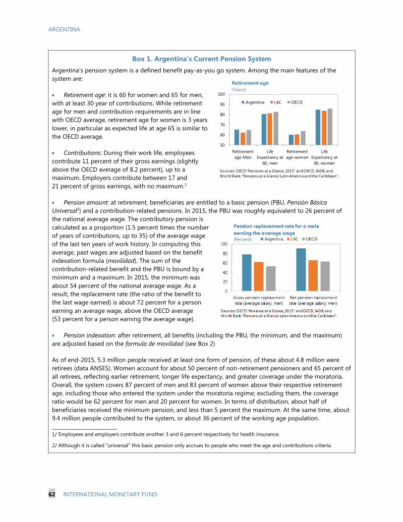
ARGENTINA


Box 1. Argentina’s Current Pension System

Argentina’s pension system is a defined benefit pay-as-you go system. Among the main features of the

system are:

Retirement age: it is 60 for women and 65 for men,

with at least 30 year of contributions. While retirement

age for men and contribution requirements are in line

with OECD average, retirement age for women is 3 years

lower, in particular as expected life at age 65 is similar to

the OECD average.

Contributions: During their work life, employees

contribute 11 percent of their gross earnings (slightly

above the OECD average of 8.2 percent), up to a

maximum. Employers contribute between 17 and

21 percent of gross earnings, with no maximum.1

Pension amount: at retirement, beneficiaries are entitled to a basic pension (PBU, Pensión Básica

Universal2) and a contribution-related pensions. In 2015, the PBU was roughly equivalent to 26 percent of

the national average wage. The contributory pension is

calculated as a proportion (1.5 percent times the number

of years of contributions, up to 35) of the average wage

of the last ten years of work history. In computing this

average, past wages are adjusted based on the benefit

indexation formula (movilidad). The sum of the

contribution-related benefit and the PBU is bound by a

minimum and a maximum. In 2015, the minimum was

about 54 percent of the national average wage. As a

result, the replacement rate (the ratio of the benefit to

the last wage earned) is about 72 percent for a person

earning an average wage, above the OECD average

(53 percent for a person earning the average wage).

Pension indexation: after retirement, all benefits (including the PBU, the minimum, and the maximum)

are adjusted based on the formula de movilidad (see Box 2)

As of end-2015, 5.3 million people received at least one form of pension, of these about 4.8 million were

retirees (data ANSES). Women account for about 50 percent of non-retirement pensioners and 65 percent of

all retirees, reflecting earlier retirement, longer life expectancy, and greater coverage under the moratoria.

Overall, the system covers 87 percent of men and 83 percent of women above their respective retirement

age, including those who entered the system under the moratoria regime; excluding them, the coverage

ratio would be 62 percent for men and 20 percent for women. In terms of distribution, about half of

beneficiaries received the minimum pension, and less than 5 percent the maximum. At the same time, about

9.4 million people contributed to the system, or about 36 percent of the working age population.

_________________________

1/ Employees and employers contribute another 3 and 6 percent respectively for health insurance.

2/ Although it is called “universal” this basic pension only accrues to people who meet the age and contributions criteria.

50

60

70

80

90

100

Retirement

age Men

Life

Expectancy at

60, men

Retirement

age women

Life

Expectancy at

60, women

Retirement age

(Years)

Argentina LAC OECD

Sources: OECD “Pensions at a Glance, 2015” and OECD, IADB, and

World Bank “Pensions at a Glance: Latin America and the Caribbean”.

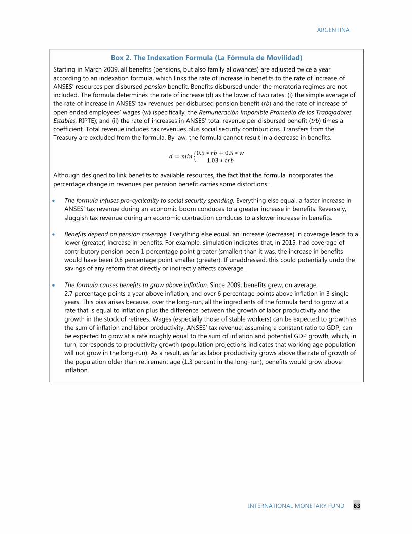
ARGENTINA


Box 2. The Indexation Formula (La Fórmula de Movilidad)

Starting in March 2009, all benefits (pensions, but also family allowances) are adjusted twice a year

according to an indexation formula, which links the rate of increase in benefits to the rate of increase of

ANSES’ resources per disbursed pension benefit. Benefits disbursed under the moratoria regimes are not

included. The formula determines the rate of increase (d) as the lower of two rates: (i) the simple average of

the rate of increase in ANSES’ tax revenues per disbursed pension benefit (rb) and the rate of increase of

open ended employees’ wages (w) (specifically, the Remuneración Imponible Promedio de los Trabajadores

Estables, RIPTE); and (ii) the rate of increases in ANSES’ total revenue per disbursed benefit (trb) times a

coefficient. Total revenue includes tax revenues plus social security contributions. Transfers from the

Treasury are excluded from the formula. By law, the formula cannot result in a decrease in benefits.

𝑑 = 𝑚𝑖𝑛 {0.5 ∗ 𝑟𝑏 + 0.5 ∗ 𝑤

1.03 ∗ 𝑡𝑟𝑏

Although designed to link benefits to available resources, the fact that the formula incorporates the

percentage change in revenues per pension benefit carries some distortions:

The formula infuses pro-cyclicality to social security spending. Everything else equal, a faster increase in

ANSES’ tax revenue during an economic boom conduces to a greater increase in benefits. Reversely,

sluggish tax revenue during an economic contraction conduces to a slower increase in benefits.

Benefits depend on pension coverage. Everything else equal, an increase (decrease) in coverage leads to a

lower (greater) increase in benefits. For example, simulation indicates that, in 2015, had coverage of

contributory pension been 1 percentage point greater (smaller) than it was, the increase in benefits

would have been 0.8 percentage point smaller (greater). If unaddressed, this could potentially undo the

savings of any reform that directly or indirectly affects coverage.

The formula causes benefits to grow above inflation. Since 2009, benefits grew, on average,

2.7 percentage points a year above inflation, and over 6 percentage points above inflation in 3 single

years. This bias arises because, over the long-run, all the ingredients of the formula tend to grow at a

rate that is equal to inflation plus the difference between the growth of labor productivity and the

growth in the stock of retirees. Wages (especially those of stable workers) can be expected to growth as

the sum of inflation and labor productivity. ANSES’ tax revenue, assuming a constant ratio to GDP, can

be expected to grow at a rate roughly equal to the sum of inflation and potential GDP growth, which, in

turn, corresponds to productivity growth (population projections indicates that working age population

will not grow in the long-run). As a result, as far as labor productivity grows above the rate of growth of

the population older than retirement age (1.3 percent in the long-run), benefits would grow above

inflation.

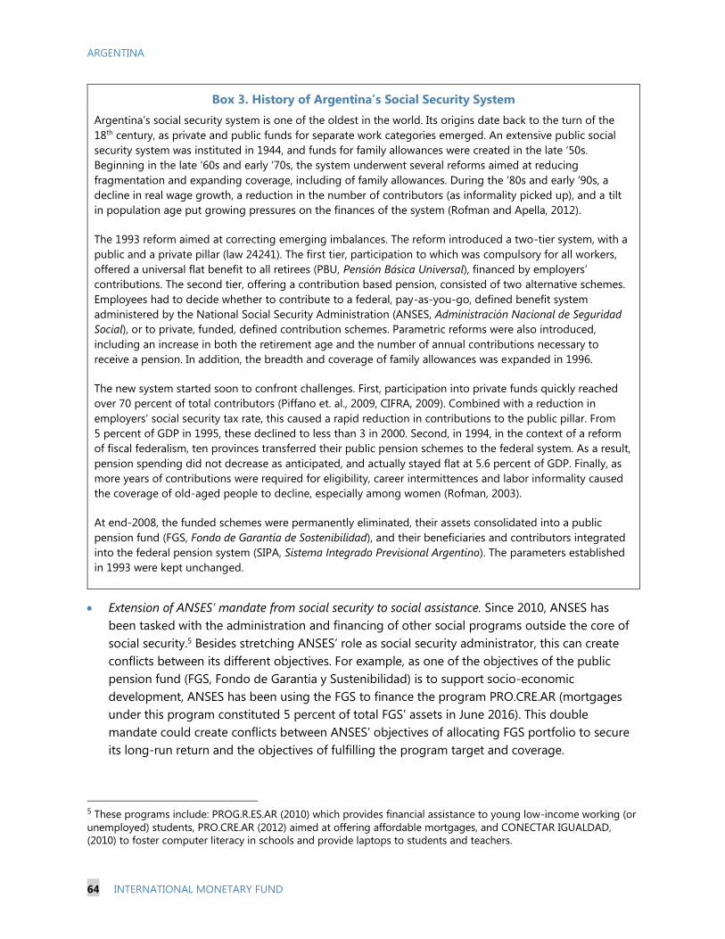
ARGENTINA


Extension of ANSES’ mandate from social security to social assistance. Since 2010, ANSES has

been tasked with the administration and financing of other social programs outside the core of

social security.5 Besides stretching ANSES’ role as social security administrator, this can create

conflicts between its different objectives. For example, as one of the objectives of the public

pension fund (FGS, Fondo de Garantia y Sustenibilidad) is to support socio-economic

development, ANSES has been using the FGS to finance the program PRO.CRE.AR (mortgages

under this program constituted 5 percent of total FGS’ assets in June 2016). This double

mandate could create conflicts between ANSES’ objectives of allocating FGS portfolio to secure

its long-run return and the objectives of fulfilling the program target and coverage.

5 These programs include: PROG.R.ES.AR (2010) which provides financial assistance to young low-income working (or

unemployed) students, PRO.CRE.AR (2012) aimed at offering affordable mortgages, and CONECTAR IGUALDAD,

(2010) to foster computer literacy in schools and provide laptops to students and teachers.

Box 3. History of Argentina’s Social Security System

Argentina’s social security system is one of the oldest in the world. Its origins date back to the turn of the

18th century, as private and public funds for separate work categories emerged. An extensive public social

security system was instituted in 1944, and funds for family allowances were created in the late ‘50s.

Beginning in the late ‘60s and early ‘70s, the system underwent several reforms aimed at reducing

fragmentation and expanding coverage, including of family allowances. During the ‘80s and early ‘90s, a

decline in real wage growth, a reduction in the number of contributors (as informality picked up), and a tilt

in population age put growing pressures on the finances of the system (Rofman and Apella, 2012).

The 1993 reform aimed at correcting emerging imbalances. The reform introduced a two-tier system, with a

public and a private pillar (law 24241). The first tier, participation to which was compulsory for all workers,

offered a universal flat benefit to all retirees (PBU, Pensión Básica Universal), financed by employers’

contributions. The second tier, offering a contribution based pension, consisted of two alternative schemes.

Employees had to decide whether to contribute to a federal, pay-as-you-go, defined benefit system

administered by the National Social Security Administration (ANSES, Administración Nacional de Seguridad

Social), or to private, funded, defined contribution schemes. Parametric reforms were also introduced,

including an increase in both the retirement age and the number of annual contributions necessary to

receive a pension. In addition, the breadth and coverage of family allowances was expanded in 1996.

The new system started soon to confront challenges. First, participation into private funds quickly reached

over 70 percent of total contributors (Piffano et. al., 2009, CIFRA, 2009). Combined with a reduction in

employers’ social security tax rate, this caused a rapid reduction in contributions to the public pillar. From

5 percent of GDP in 1995, these declined to less than 3 in 2000. Second, in 1994, in the context of a reform

of fiscal federalism, ten provinces transferred their public pension schemes to the federal system. As a result,

pension spending did not decrease as anticipated, and actually stayed flat at 5.6 percent of GDP. Finally, as

more years of contributions were required for eligibility, career intermittences and labor informality caused

the coverage of old-aged people to decline, especially among women (Rofman, 2003).

At end-2008, the funded schemes were permanently eliminated, their assets consolidated into a public

pension fund (FGS, Fondo de Garantía de Sostenibilidad), and their beneficiaries and contributors integrated

into the federal pension system (SIPA, Sistema Integrado Previsional Argentino). The parameters established

in 1993 were kept unchanged.

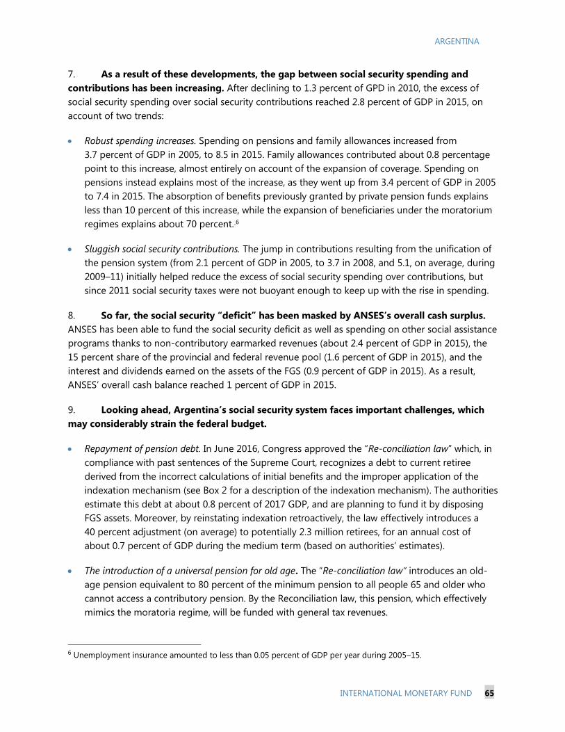
ARGENTINA


7. As a result of these developments, the gap between social security spending and

contributions has been increasing. After declining to 1.3 percent of GPD in 2010, the excess of

social security spending over social security contributions reached 2.8 percent of GDP in 2015, on

account of two trends:

Robust spending increases. Spending on pensions and family allowances increased from

3.7 percent of GDP in 2005, to 8.5 in 2015. Family allowances contributed about 0.8 percentage

point to this increase, almost entirely on account of the expansion of coverage. Spending on

pensions instead explains most of the increase, as they went up from 3.4 percent of GDP in 2005

to 7.4 in 2015. The absorption of benefits previously granted by private pension funds explains

less than 10 percent of this increase, while the expansion of beneficiaries under the moratorium

regimes explains about 70 percent. 6

Sluggish social security contributions. The jump in contributions resulting from the unification of

the pension system (from 2.1 percent of GDP in 2005, to 3.7 in 2008, and 5.1, on average, during

2009–11) initially helped reduce the excess of social security spending over contributions, but

since 2011 social security taxes were not buoyant enough to keep up with the rise in spending.

8. So far, the social security “deficit” has been masked by ANSES’s overall cash surplus.

ANSES has been able to fund the social security deficit as well as spending on other social assistance

programs thanks to non-contributory earmarked revenues (about 2.4 percent of GDP in 2015), the

15 percent share of the provincial and federal revenue pool (1.6 percent of GDP in 2015), and the

interest and dividends earned on the assets of the FGS (0.9 percent of GDP in 2015). As a result,

ANSES’ overall cash balance reached 1 percent of GDP in 2015.

9. Looking ahead, Argentina’s social security system faces important challenges, which

may considerably strain the federal budget.

Repayment of pension debt. In June 2016, Congress approved the “Re-conciliation law” which, in

compliance with past sentences of the Supreme Court, recognizes a debt to current retiree

derived from the incorrect calculations of initial benefits and the improper application of the

indexation mechanism (see Box 2 for a description of the indexation mechanism). The authorities

estimate this debt at about 0.8 percent of 2017 GDP, and are planning to fund it by disposing

FGS assets. Moreover, by reinstating indexation retroactively, the law effectively introduces a

40 percent adjustment (on average) to potentially 2.3 million retirees, for an annual cost of

about 0.7 percent of GDP during the medium term (based on authorities’ estimates).

The introduction of a universal pension for old age. The “Re-conciliation law” introduces an old-

age pension equivalent to 80 percent of the minimum pension to all people 65 and older who

cannot access a contributory pension. By the Reconciliation law, this pension, which effectively

mimics the moratoria regime, will be funded with general tax revenues.

6 Unemployment insurance amounted to less than 0.05 percent of GDP per year during 2005–15.

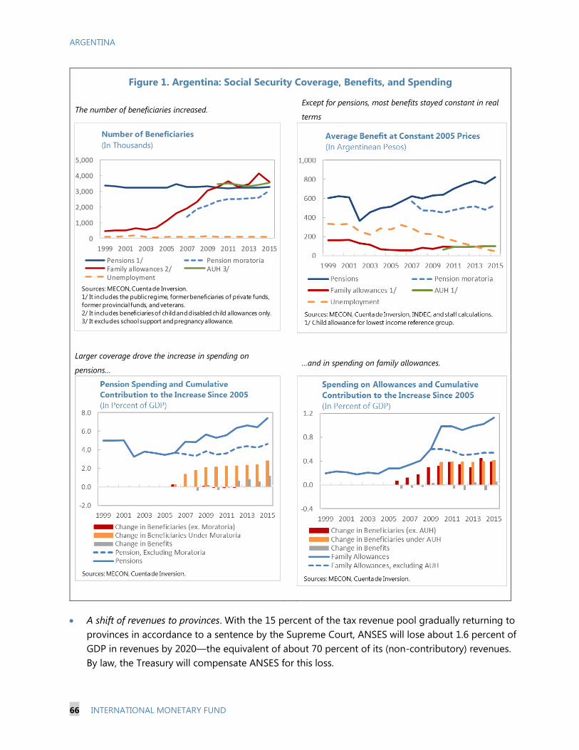
ARGENTINA


Figure 1. Argentina: Social Security Coverage, Benefits, and Spending

The number of beneficiaries increased. Except for pensions, most benefits stayed constant in real

terms

Larger coverage drove the increase in spending on

pensions… …and in spending on family allowances.

A shift of revenues to provinces. With the 15 percent of the tax revenue pool gradually returning to

provinces in accordance to a sentence by the Supreme Court, ANSES will lose about 1.6 percent of

GDP in revenues by 2020—the equivalent of about 70 percent of its (non-contributory) revenues.

By law, the Treasury will compensate ANSES for this loss.

0

1,000

2,000

3,000

4,000

5,000

1999 2001 2003 2005 2007 2009 2011 2013 2015

Number of Beneficiaries

(In Thousands)

Pensions 1/ Pension moratoriaFamily allowances 2/ AUH 3/Unemployment

Sources: MECON, Cuenta de Inversion.

1/ It includes the public regime, former beneficiaries of private funds,

former provincial funds, and veterans.

2/ It includes beneficiaries of child and disabled child allowances only.

3/ It excludes school support and pregnancy allowance.

ARGENTINA


Population aging. The old-age dependency ratio (the share of population 60 and older to

working age population) is expected to double in the next 50 years, reaching 52 percent.

10. Under current policies and challenges ahead, the social security “deficit” and ANSES’

overall balance would deteriorate significantly over the long run, driven by pensions. We

project ANSES balances using a model that incorporates the specific features of Argentina’s pension

and family allowance system, projection of population dynamic from the UN Population Survey, and

long-run macroeconomic assumptions (see Annex I for more details on the model):

spending on family allowances will slowly decline to 0.5 percent of GDP by 2066, as the share of

children to total working populations declines; 7

spending on contributory pensions will reach 8.2 percent of GDP by 2026 and almost 10 percent

of GDP by 2066;

spending on old-age pension will have an annual cost of 0.4 percent of GDP, on average, in the

medium term, and slightly less than 2 percent of GDP in the long run;

social security contributions will slightly increase to 6.1 percent of GDP by 2026 but decline to

4.7 percent of GDP by 2066, as the growth of the working age populations declines to zero.

In particular, the cumulative increase in the pension “deficit” (the difference between contributory

pensions and social security contributions) over the next 50 years is estimated to be large, about

40 percent of 2015 GDP in net present value (NPV) terms (Figure), well above FGS’ financial assets

(estimated at 12 percent of GDP in 2016).

C. Reform Proposals

11. Correcting this imbalance would require a reform of Argentina’s current pension

system. This may include some of the following measures:

Change in indexation formula. Indexing benefits (and actualizing past wages) only to realized

inflation would still allow retirees to preserve the real value of their benefit, but it would reduce

the increase in pension spending by about 20 percent of GDP in NPV terms on account of two

effects: benefits would increase slower, and initial benefits would be slightly lower.

7 Spending on child allowances is by far the greatest among all family allowances.

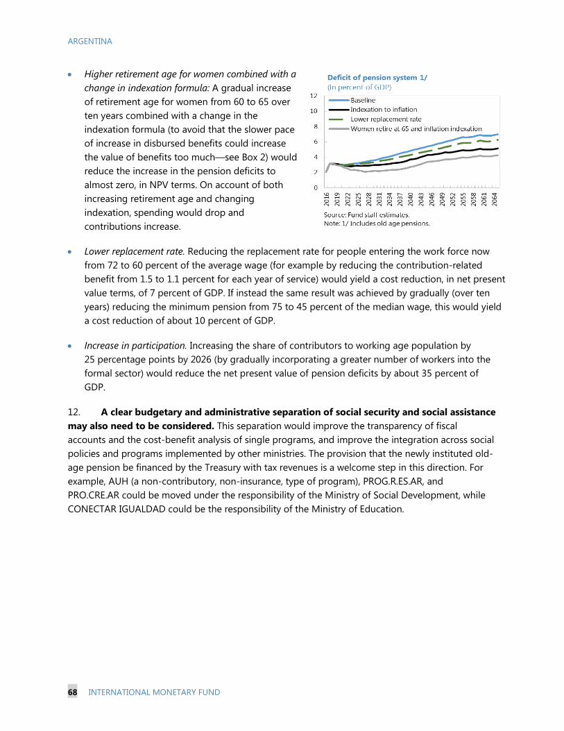
ARGENTINA


Higher retirement age for women combined with a

change in indexation formula: A gradual increase

of retirement age for women from 60 to 65 over

ten years combined with a change in the

indexation formula (to avoid that the slower pace

of increase in disbursed benefits could increase

the value of benefits too much—see Box 2) would

reduce the increase in the pension deficits to

almost zero, in NPV terms. On account of both

increasing retirement age and changing

indexation, spending would drop and

contributions increase.

Lower replacement rate. Reducing the replacement rate for people entering the work force now

from 72 to 60 percent of the average wage (for example by reducing the contribution-related

benefit from 1.5 to 1.1 percent for each year of service) would yield a cost reduction, in net present

value terms, of 7 percent of GDP. If instead the same result was achieved by gradually (over ten

years) reducing the minimum pension from 75 to 45 percent of the median wage, this would yield

a cost reduction of about 10 percent of GDP.

Increase in participation. Increasing the share of contributors to working age population by

25 percentage points by 2026 (by gradually incorporating a greater number of workers into the

formal sector) would reduce the net present value of pension deficits by about 35 percent of

GDP.

12. A clear budgetary and administrative separation of social security and social assistance

may also need to be considered. This separation would improve the transparency of fiscal

accounts and the cost-benefit analysis of single programs, and improve the integration across social

policies and programs implemented by other ministries. The provision that the newly instituted old-

age pension be financed by the Treasury with tax revenues is a welcome step in this direction. For

example, AUH (a non-contributory, non-insurance, type of program), PROG.R.ES.AR, and

PRO.CRE.AR could be moved under the responsibility of the Ministry of Social Development, while

CONECTAR IGUALDAD could be the responsibility of the Ministry of Education.

ARGENTINA


References

Betranou, Fabio, Luis Casanova, Maribel Jimenez, and Monica Jimenez, 2014, “Informality and

employment quality in Argentina: Country case study on labour market segmentation” ILO,

Conditions of Work and Employment Series No. 49.

CIFRA, 2009, “La Evolución del Sistema Previsional Argentino”, Documento de Trabajo No. 2.

Lustig, Nora, and Carola Pessino, 2014, “Social Spending and Income Redistribution in Argentina

during the 2000s: The Increasing Role of Noncontributory Pensions”, Public Finance Review,

Vol. 42(3).

MECON, 2015, “Informe Trimestral de Ejecución Físico Financiera, Cuarto Trimestre 2015”

Piffano, Horacio L.P., Agustín Lódola, Humberto Silva, and Diego Sánchez, 2009 “El Sistema

Previsional Argentino en una Perspectiva Comparada”, Departamento de Economía Facultad

de Ciencias Económicas Universidad Nacional de La Plata, Proyecto E083.

Rofman, Rafael, 2003, “El Sistema Previsional y la Crisis de la Argentina”, World Bank, Working

Document 7/03.

Rofman, Rafael, and Ignacio Apella, 2015, “Argentina” chapter 2 in “Beyond Contributory Pensions

Fourteen Experiences with Coverage Expansion in Latin America”, edited by Rofman, Rafael,

Ignacio Apella, and Evelyn Vezza, World Bank.

UNDP, 2014, “Human Development Report 2014: Sustaining Human Progress, Reducing

Vulnerabilities and Building Resilience”.

World Bank, 2008, “Argentina. Labor Market Study. Informal Employment in Argentina: Causes and

Consequence”, Report No. 36092-AR.

ARGENTINA


Annex I. The Model

We project ANSES balance over the next 50 years based on population projections from the ILO

and the UN to determine the mass of potential participants and beneficiaries, macroeconomic

assumptions to determine ANSES’ tax revenue and social security contributions, and the current

parameters of Argentina’s pension system to determine benefits. We calibrate other ratios (for

example, coverage and participation) to past data from ANSES’ social security statistics,

MECON’s physical and financial account (Cuenta de Inversión), and INDEC (unemployment,

income distribution, and population statistics).

The assumption underlying our long-term pension projections are:

Population dynamic. We use population projections from the ILO and the UN and assume

that the end-2015 stock of pensioners will decrease according to current mortality rates. The

implied old dependency ratio (the ratio of people 60 and older to those with age 15–59)

doubles in 50 years, from 26.3 percent in 2016 to 51.7 percent in 2066.

Macroeconomic assumptions. We assume real GDP growth rate, the GDP deflator, and

inflation rate will have converged by 2026 to their long-run levels. We assume that long-run

GDP growth is 3.3 percent, inflation and the growth in the GDP deflator 5 percent, and that

productivity growth will be 2.3 percent, that is about 70 percent of the real GDP-working age

population growth differential. As a result, wages are assumed to growth 7.4 percent over

the long run. Finally, we assume a real interest rate growth differential of 2.5 percent.

Programs coverage. We use past data to calibrate the coverage of all family allowances to

population below 21, which has remained fairly stable in the past 3 years. For contributory

retirement pensions, we assume that coverage for each new future cohort of men and

women reaching retirement age will be the same as in 2015, excluding those who received a

benefit under the moratoria regimes. We assume that all people above the age of 65 who

do not receive a contributory pension will receive the pension for old age.1 Finally, we use

past data to calibrate the coverage of other pensions to total population and assume that

this will remain at 2015 levels.

Indexation. We compute the indexation formula on our projections of wages, ANSES’ tax and

total revenues, and number of beneficiaries.

Pension spending. We calibrate pension benefits on contributors’ average wage. For each

cohort, we index wages of the past ten years using the result of the indexation formula.

Finally, we assume 30 years of contributions and derive the initial pension benefit. We use

1 However, reflecting the extension of the moratoria regime for women between the age of 60 and 65 until 2019, we

assume that during 2016–19 all women above age 60 who do not receive a contributory pension will receive the old-

age pension.

ARGENTINA


the indexation formula to increase 2015 benefits (for current beneficiaries) and future initial

benefit (for each new cohort of beneficiaries). To account for the effect of the June 2016 Re-

conciliation law, we calibrate the 2017 increase in current benefits to the adjustment cost

estimated by the authorities (around 60 million pesos); and decrease FGS assets by a total of

83 million pesos over 3 years.2

Social security contributions and tax revenue. We increase social security contributions by the

increase of wages and of working age population. We assume that ANSES tax revenue will

remain constant in percent of GDP over the long run.

Other assumptions. We assume that the return rate on FGS assets will remain at current level,

with a capital gain on FGS assets at about 5 percent in real terms. We assume that the

Treasury will fully compensate ANSES for its share of the federal-provincial revenue pool.

Finally, we assume that operating costs and the cost of other social assistance program will

remain constant in percent of GDP.

2 The Re-conciliation law establishes that half of past obligations will be paid at settlement. The remainder will be

paid in quotas over 3 years, but the amount due would be updated using the pension indexation formula.

ARGENTINA


DISINFLATION UNDER INFLATION TARGETING: A

SMALL MACRO MODEL FOR ARGENTINA1

1. The Argentine administration that took power in December 2015 has announced a

gradual disinflation to single digits by the end of its mandate in 2019. The starting point has

been one of the highest inflation levels in the world. Despite the issues in measurement, using a

variety of indicators (both public and private) shows that inflation in the city of BA rose sharply from

single digits in 2007 and stabilized between 25 and 35 percent (y/y) during 2009 and 2015, with

inflation expectations well anchored within that range.2 To a large extent this reflects the earlier

administration’s decision to fund the large increase in public sector spending with an inflation tax.

Inflation in early 2016 spiked to above 40 percent (y/y using the city of BA CPI index) reflecting the

normalization of utilities tariffs needed to phase off energy subsidies, and the sharp depreciation

following the removal of ER controls and unification of ER markets in late 2015. Since April 2016, real

interest rates have remained positive and core inflation has been on a declining trend, while the

economy has moved into recession.

2. To build credibility and align inflation expectations with the new objectives, the

government formally launched the inflation targeting framework in September 2016. The

intention and timetable to move in this direction was announced early in 2016 and, in May 2016, the

BCRA switched to interest rate from money targets as operational variables of monetary policy

(Figure 1). In addition, the national statistics agency has resumed publication of credible data on

inflation, against which the 12–17 percent target for 2017 will be measured. A companion SIP further

describes the operational aspects of the current conduct of monetary policy and the steps that are

needed to make further progress on the way to inflation targeting (Jacome, forthcoming).

3. This paper uses a neo-Keynesian type model to analyze the policy challenges and

tradeoffs involved in the disinflation process. In embarking on a disinflation process under a new

inflation targeting framework, Argentina would need to develop tools for assessing the stance of

monetary policy and set policy interest rates. In this paper, we estimate a standard small

macroeconomic model, similar to the one used by a number of inflation-targeting central banks for

forecasting and policy analysis purposes, and close to the BCRA’s small macroeconomic model

(Escudé and others, 2007). Despite its simplicity, and while it abstracts from many important

features of the economy, the model captures the key channels of monetary policy transmission and

allows discussing the main tradeoffs involved in monetary policy making. In particular, it allows to

answer questions such as: How should the path of interest rates look like in order to reduce inflation

to a single digit figure in 2019? What is the output cost that could be associated with the

disinflation process announced by the authorities? What can moderate this cost?

1 Prepared by Jorge Ivan Canales-Kriljenko.

2 Large discrepancies between official inflation statistics at the national level and private sector and provincial

estimates suggests significant uncertainty about the measurement of inflation since late 2006. This study uses a

consumer price series concatenated from private and provincial sources as later described.

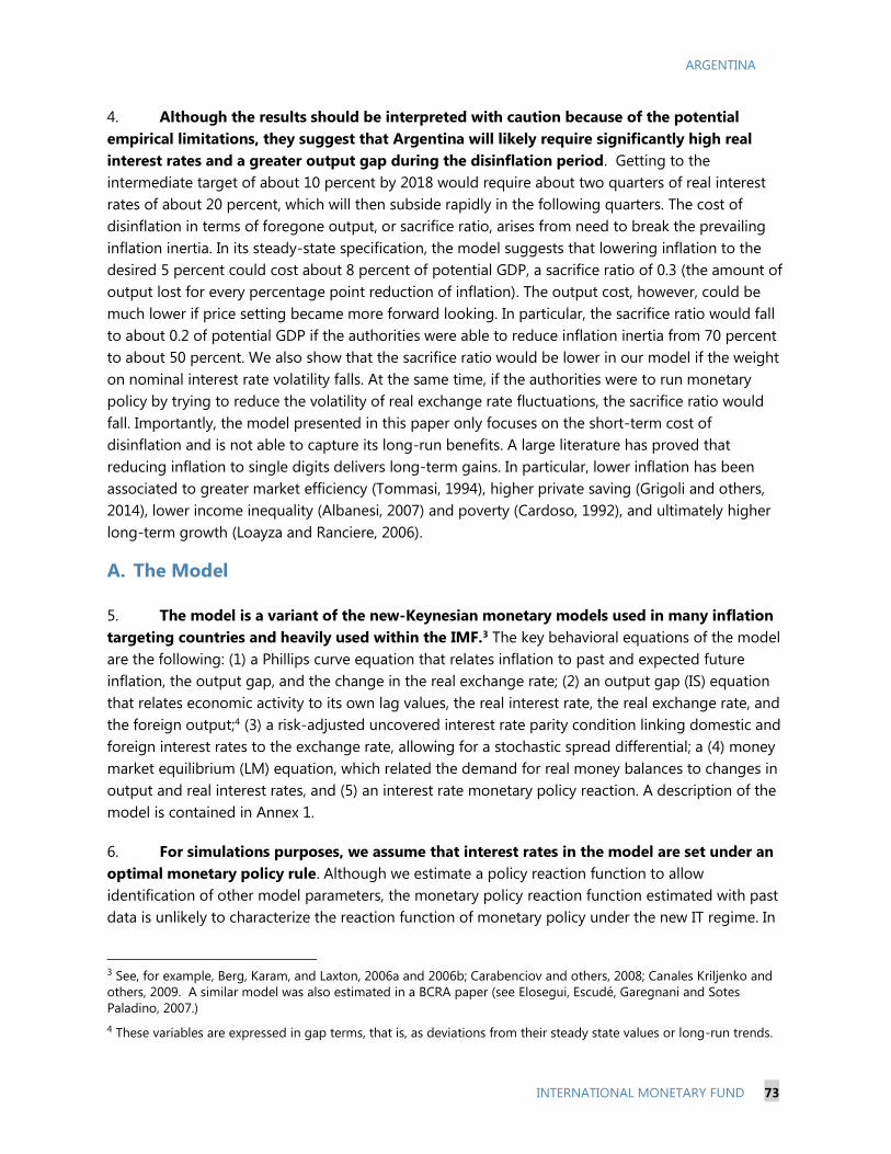
ARGENTINA


4. Although the results should be interpreted with caution because of the potential

empirical limitations, they suggest that Argentina will likely require significantly high real

interest rates and a greater output gap during the disinflation period. Getting to the

intermediate target of about 10 percent by 2018 would require about two quarters of real interest

rates of about 20 percent, which will then subside rapidly in the following quarters. The cost of

disinflation in terms of foregone output, or sacrifice ratio, arises from need to break the prevailing

inflation inertia. In its steady-state specification, the model suggests that lowering inflation to the

desired 5 percent could cost about 8 percent of potential GDP, a sacrifice ratio of 0.3 (the amount of

output lost for every percentage point reduction of inflation). The output cost, however, could be

much lower if price setting became more forward looking. In particular, the sacrifice ratio would fall

to about 0.2 of potential GDP if the authorities were able to reduce inflation inertia from 70 percent

to about 50 percent. We also show that the sacrifice ratio would be lower in our model if the weight

on nominal interest rate volatility falls. At the same time, if the authorities were to run monetary

policy by trying to reduce the volatility of real exchange rate fluctuations, the sacrifice ratio would

fall. Importantly, the model presented in this paper only focuses on the short-term cost of

disinflation and is not able to capture its long-run benefits. A large literature has proved that

reducing inflation to single digits delivers long-term gains. In particular, lower inflation has been

associated to greater market efficiency (Tommasi, 1994), higher private saving (Grigoli and others,

2014), lower income inequality (Albanesi, 2007) and poverty (Cardoso, 1992), and ultimately higher

long-term growth (Loayza and Ranciere, 2006).

A. The Model

5. The model is a variant of the new-Keynesian monetary models used in many inflation

targeting countries and heavily used within the IMF.3 The key behavioral equations of the model

are the following: (1) a Phillips curve equation that relates inflation to past and expected future

inflation, the output gap, and the change in the real exchange rate; (2) an output gap (IS) equation

that relates economic activity to its own lag values, the real interest rate, the real exchange rate, and

the foreign output;4 (3) a risk-adjusted uncovered interest rate parity condition linking domestic and

foreign interest rates to the exchange rate, allowing for a stochastic spread differential; a (4) money

market equilibrium (LM) equation, which related the demand for real money balances to changes in

output and real interest rates, and (5) an interest rate monetary policy reaction. A description of the

model is contained in Annex 1.

6. For simulations purposes, we assume that interest rates in the model are set under an

optimal monetary policy rule. Although we estimate a policy reaction function to allow

identification of other model parameters, the monetary policy reaction function estimated with past

data is unlikely to characterize the reaction function of monetary policy under the new IT regime. In

3 See, for example, Berg, Karam, and Laxton, 2006a and 2006b; Carabenciov and others, 2008; Canales Kriljenko and

others, 2009. A similar model was also estimated in a BCRA paper (see Elosegui, Escudé, Garegnani and Sotes

Paladino, 2007.)

4 These variables are expressed in gap terms, that is, as deviations from their steady state values or long-run trends.

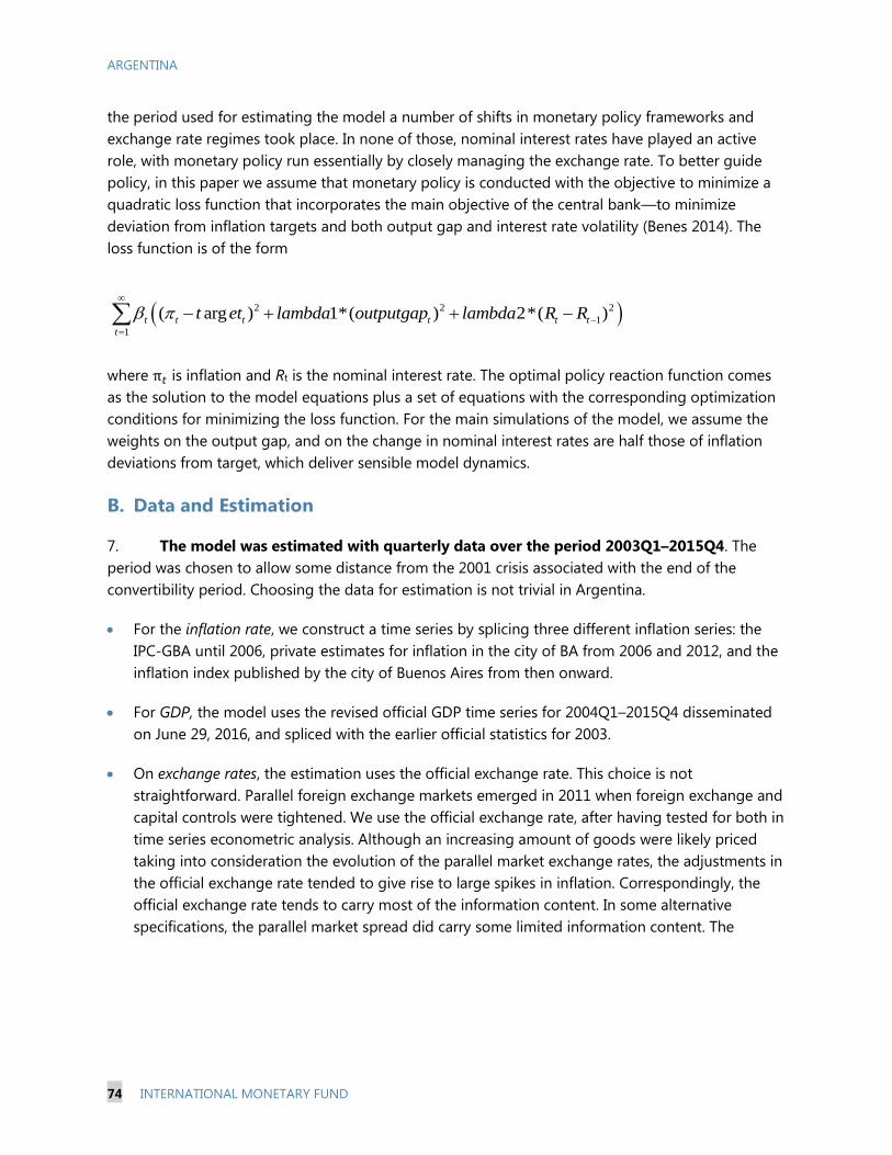
ARGENTINA


the period used for estimating the model a number of shifts in monetary policy frameworks and

exchange rate regimes took place. In none of those, nominal interest rates have played an active

role, with monetary policy run essentially by closely managing the exchange rate. To better guide

policy, in this paper we assume that monetary policy is conducted with the objective to minimize a

quadratic loss function that incorporates the main objective of the central bank—to minimize

deviation from inflation targets and both output gap and interest rate volatility (Benes 2014). The

loss function is of the form

where π𝑡 is inflation and Rt is the nominal interest rate. The optimal policy reaction function comes

as the solution to the model equations plus a set of equations with the corresponding optimization

conditions for minimizing the loss function. For the main simulations of the model, we assume the

weights on the output gap, and on the change in nominal interest rates are half those of inflation

deviations from target, which deliver sensible model dynamics.

B. Data and Estimation

7. The model was estimated with quarterly data over the period 2003Q1–2015Q4. The

period was chosen to allow some distance from the 2001 crisis associated with the end of the

convertibility period. Choosing the data for estimation is not trivial in Argentina.

For the inflation rate, we construct a time series by splicing three different inflation series: the

IPC-GBA until 2006, private estimates for inflation in the city of BA from 2006 and 2012, and the

inflation index published by the city of Buenos Aires from then onward.

For GDP, the model uses the revised official GDP time series for 2004Q1–2015Q4 disseminated

on June 29, 2016, and spliced with the earlier official statistics for 2003.

On exchange rates, the estimation uses the official exchange rate. This choice is not

straightforward. Parallel foreign exchange markets emerged in 2011 when foreign exchange and

capital controls were tightened. We use the official exchange rate, after having tested for both in

time series econometric analysis. Although an increasing amount of goods were likely priced

taking into consideration the evolution of the parallel market exchange rates, the adjustments in

the official exchange rate tended to give rise to large spikes in inflation. Correspondingly, the

official exchange rate tends to carry most of the information content. In some alternative

specifications, the parallel market spread did carry some limited information content. The

2 2 2

1

1

( arg ) 1*( ) 2*( )t t t t t t

t

t et lambda outputgap lambda R R

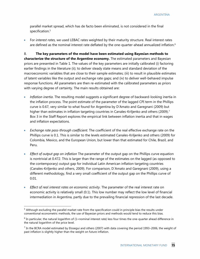
ARGENTINA


parallel market spread, which has de facto been eliminated, is not considered in the final

specification.5

For interest rates, we used LEBAC rates weighted by their maturity structure. Real interest rates

are defined as the nominal interest rate deflated by the one-quarter-ahead annualized inflation.6

8. The key parameters of the model have been estimated using Bayesian methods to

characterize the structure of the Argentine economy. The estimated parameters and Bayesian

priors are presented in Table 1. The values of the key parameters are initially calibrated (i) factoring

earlier findings in the literature (ii); to deliver steady state means and standard deviation of the

macroeconomic variables that are close to their sample estimates; (iii) to result in plausible estimates

of latent variables like the output and exchange rate gaps; and (iv) to deliver well-behaved impulse

response functions. All parameters are then re-estimated with the calibrated parameters as priors

with varying degree of certainty. The main results obtained are:

Inflation inertia. The resulting model suggests a significant degree of backward-looking inertia in

the inflation process. The point estimate of the parameter of the lagged CPI term in the Phillips

curve is 0.67, very similar to what found for Argentina by D’Amato and Garegnani (2009) but

higher than estimates in inflation targeting countries in Canales-Kriljenko and others (2009).7

Box 3 in the Staff Report explores the empirical link between inflation inertia and that in wages

and inflation expectations.

Exchange rate pass-through coefficient. The coefficient of the real effective exchange rate on the

Phillips curve is 0.1. This is similar to the levels estimated Canales-Kriljenko and others (2009) for

Colombia, Mexico, and the European Union, but lower than that estimated for Chile, Brazil, and

Peru.

Effect of output gap on inflation The parameter of the output gap on the Phillips curve equation

is nontrivial at 0.472. This is larger than the range of the estimates on the lagged (as opposed to

the contemporary) output gap for individual Latin American inflation targeting countries

(Canales-Kriljenko and others, 2009). For comparison, D´Amato and Garegnani (2009), using a

different methodology, find a very small coefficient of the output gap on the Phillips curve of

0.01.

Effect of real interest rates on economic activity. The parameter of the real interest rate on

economic activity is relatively small (0.1). This low number may reflect the low level of financial

intermediation in Argentina, partly due to the prevailing financial repression of the last decade.

5 Although excluding the parallel market rate from the specification could in principle bias the results under

conventional econometric methods, the use of Bayesian priors and methods would tend to reduce this bias.

6 In particular, the natural logarithm of (1+nominal interest rate) less four times the one-quarter ahead difference in

the natural logarithm of the price level.

7 In the BCRA model estimated by Elosegui and others (2007) with data covering the period 1993–2006, the weight of

past inflation is slightly higher than the weight on future inflation.

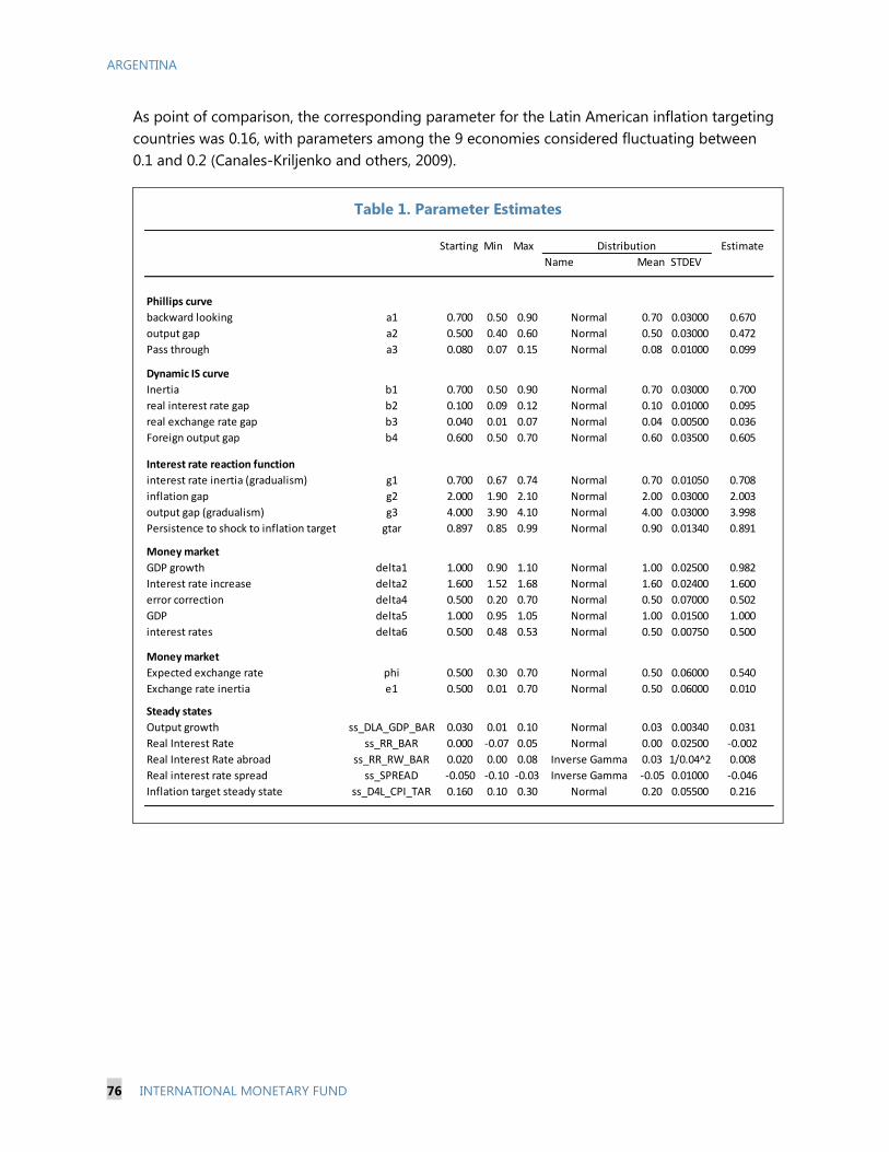
ARGENTINA


As point of comparison, the corresponding parameter for the Latin American inflation targeting

countries was 0.16, with parameters among the 9 economies considered fluctuating between

0.1 and 0.2 (Canales-Kriljenko and others, 2009).

Table 1. Parameter Estimates

Starting Min Max Distribution Estimate

Name Mean STDEV

Phillips curve

backward looking a1 0.700 0.50 0.90 Normal 0.70 0.03000 0.670

output gap a2 0.500 0.40 0.60 Normal 0.50 0.03000 0.472

Pass through a3 0.080 0.07 0.15 Normal 0.08 0.01000 0.099

Dynamic IS curve

Inertia b1 0.700 0.50 0.90 Normal 0.70 0.03000 0.700

real interest rate gap b2 0.100 0.09 0.12 Normal 0.10 0.01000 0.095

real exchange rate gap b3 0.040 0.01 0.07 Normal 0.04 0.00500 0.036

Foreign output gap b4 0.600 0.50 0.70 Normal 0.60 0.03500 0.605

Interest rate reaction function

interest rate inertia (gradualism) g1 0.700 0.67 0.74 Normal 0.70 0.01050 0.708

inflation gap g2 2.000 1.90 2.10 Normal 2.00 0.03000 2.003

output gap (gradualism) g3 4.000 3.90 4.10 Normal 4.00 0.03000 3.998

Persistence to shock to inflation target gtar 0.897 0.85 0.99 Normal 0.90 0.01340 0.891

Money market

GDP growth delta1 1.000 0.90 1.10 Normal 1.00 0.02500 0.982

Interest rate increase delta2 1.600 1.52 1.68 Normal 1.60 0.02400 1.600

error correction delta4 0.500 0.20 0.70 Normal 0.50 0.07000 0.502

GDP delta5 1.000 0.95 1.05 Normal 1.00 0.01500 1.000

interest rates delta6 0.500 0.48 0.53 Normal 0.50 0.00750 0.500

Money market

Expected exchange rate phi 0.500 0.30 0.70 Normal 0.50 0.06000 0.540

Exchange rate inertia e1 0.500 0.01 0.70 Normal 0.50 0.06000 0.010

Steady states

Output growth ss_DLA_GDP_BAR 0.030 0.01 0.10 Normal 0.03 0.00340 0.031

Real Interest Rate ss_RR_BAR 0.000 -0.07 0.05 Normal 0.00 0.02500 -0.002

Real Interest Rate abroad ss_RR_RW_BAR 0.020 0.00 0.08 Inverse Gamma 0.03 1/0.04^2 0.008

Real interest rate spread ss_SPREAD -0.050 -0.10 -0.03 Inverse Gamma -0.05 0.01000 -0.046

Inflation target steady state ss_D4L_CPI_TAR 0.160 0.10 0.30 Normal 0.20 0.05500 0.216

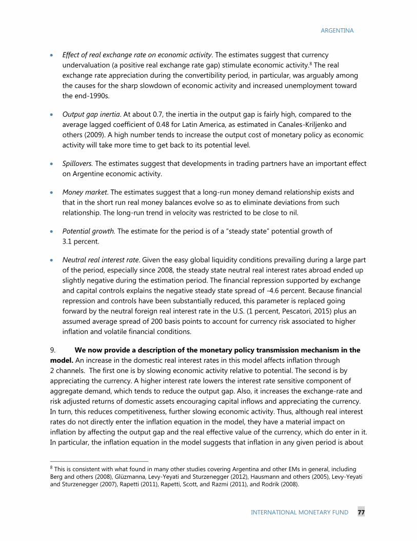
ARGENTINA


Effect of real exchange rate on economic activity. The estimates suggest that currency

undervaluation (a positive real exchange rate gap) stimulate economic activity.8 The real

exchange rate appreciation during the convertibility period, in particular, was arguably among

the causes for the sharp slowdown of economic activity and increased unemployment toward

the end-1990s.

Output gap inertia. At about 0.7, the inertia in the output gap is fairly high, compared to the

average lagged coefficient of 0.48 for Latin America, as estimated in Canales-Kriljenko and

others (2009). A high number tends to increase the output cost of monetary policy as economic

activity will take more time to get back to its potential level.

Spillovers. The estimates suggest that developments in trading partners have an important effect

on Argentine economic activity.

Money market. The estimates suggest that a long-run money demand relationship exists and

that in the short run real money balances evolve so as to eliminate deviations from such

relationship. The long-run trend in velocity was restricted to be close to nil.

Potential growth. The estimate for the period is of a “steady state” potential growth of

3.1 percent.

Neutral real interest rate. Given the easy global liquidity conditions prevailing during a large part

of the period, especially since 2008, the steady state neutral real interest rates abroad ended up

slightly negative during the estimation period. The financial repression supported by exchange

and capital controls explains the negative steady state spread of -4.6 percent. Because financial

repression and controls have been substantially reduced, this parameter is replaced going

forward by the neutral foreign real interest rate in the U.S. (1 percent, Pescatori, 2015) plus an

assumed average spread of 200 basis points to account for currency risk associated to higher

inflation and volatile financial conditions.

9. We now provide a description of the monetary policy transmission mechanism in the

model. An increase in the domestic real interest rates in this model affects inflation through

2 channels. The first one is by slowing economic activity relative to potential. The second is by

appreciating the currency. A higher interest rate lowers the interest rate sensitive component of

aggregate demand, which tends to reduce the output gap. Also, it increases the exchange-rate and

risk adjusted returns of domestic assets encouraging capital inflows and appreciating the currency.

In turn, this reduces competitiveness, further slowing economic activity. Thus, although real interest

rates do not directly enter the inflation equation in the model, they have a material impact on

inflation by affecting the output gap and the real effective value of the currency, which do enter in it.

In particular, the inflation equation in the model suggests that inflation in any given period is about

8 This is consistent with what found in many other studies covering Argentina and other EMs in general, including

Berg and others (2008), Glüzmanna, Levy-Yeyati and Sturzenegger (2012), Hausmann and others (2005), Levy-Yeyati

and Sturzenegger (2007), Rapetti (2011), Rapetti, Scott, and Razmi (2011), and Rodrik (2008).

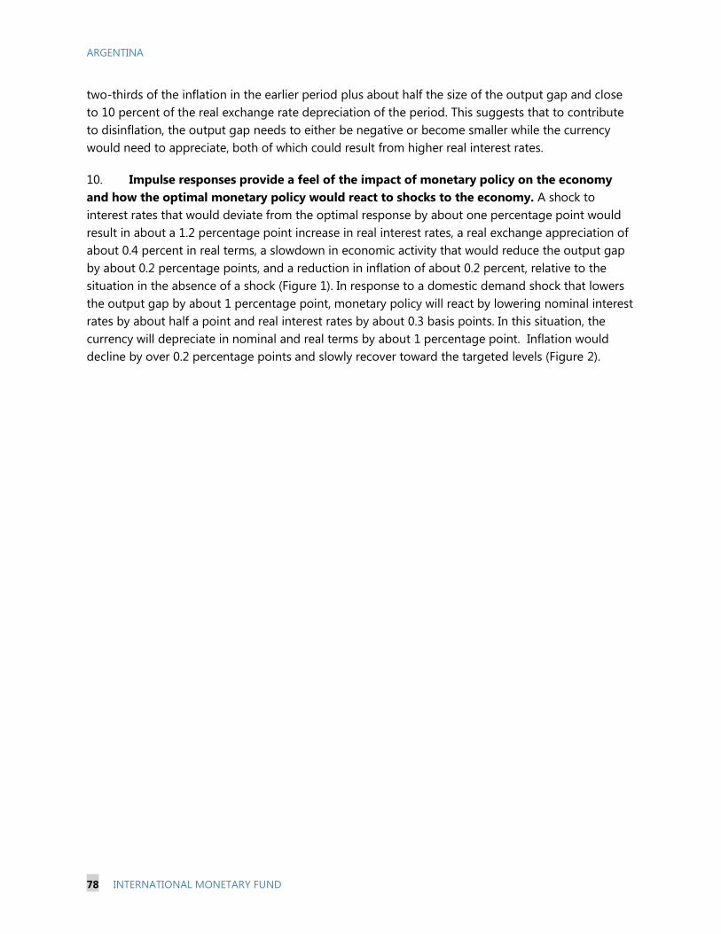
ARGENTINA


two-thirds of the inflation in the earlier period plus about half the size of the output gap and close

to 10 percent of the real exchange rate depreciation of the period. This suggests that to contribute

to disinflation, the output gap needs to either be negative or become smaller while the currency

would need to appreciate, both of which could result from higher real interest rates.

10. Impulse responses provide a feel of the impact of monetary policy on the economy

and how the optimal monetary policy would react to shocks to the economy. A shock to

interest rates that would deviate from the optimal response by about one percentage point would

result in about a 1.2 percentage point increase in real interest rates, a real exchange appreciation of

about 0.4 percent in real terms, a slowdown in economic activity that would reduce the output gap

by about 0.2 percentage points, and a reduction in inflation of about 0.2 percent, relative to the

situation in the absence of a shock (Figure 1). In response to a domestic demand shock that lowers

the output gap by about 1 percentage point, monetary policy will react by lowering nominal interest

rates by about half a point and real interest rates by about 0.3 basis points. In this situation, the

currency will depreciate in nominal and real terms by about 1 percentage point. Inflation would

decline by over 0.2 percentage points and slowly recover toward the targeted levels (Figure 2).

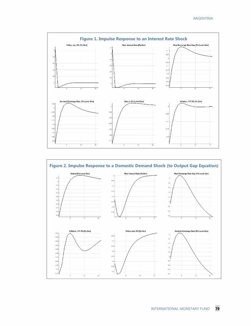
ARGENTINA


Figure 2. Impulse Response to a Domestic Demand Shock (to Output Gap Equation)

Figure 1. Impulse Response to an Interest Rate Shock

ARGENTINA


C. Implications for Monetary Policy

11. Lowering inflation in our model comes with a loss in economic activity, as measured

by the sacrifice ratio. In particular, the sacrifice ratio measures the average percent output loss

relative to potential for each percentage point reduction in inflation. Following Benes (2014), we

estimate the sacrifice ratio by first computing the steady state inflation for a 30 percent inflation

target (the level of expected inflation prevailing over the last five years). We then compute another

model with an inflation target of 5 percent, as envisaged by the authorities by 2019. Next, we

simulate the transition to the new model starting from the steady state of the model with 30 percent

and compute the cumulative sum of negative output gaps (Figure 3). This percent output loss is

then divided by the 25 percentage point reduction in inflation. The exercise suggests the

permanently lowering inflation to 5 percent from 30 percent in 5 years would come at a cumulative

output cost of 8 percent of potential output. Thus, the sacrifice ratio would be of 0.3 percentage

points of potential output loss for each percentage point permanent decline in inflation.

Figure 3. Argentine Disinflation Path with Optimal Policy Rule

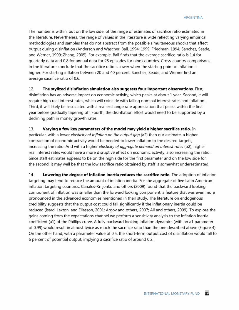
ARGENTINA


The number is within, but on the low side, of the range of estimates of sacrifice ratio estimated in

the literature. Nevertheless, the range of values in the literature is wide reflecting varying empirical

methodologies and samples that do not abstract from the possible simultaneous shocks that affect

output during disinflation (Anderson and Wascher, Ball, 1994; 1999; Friedman, 1994; Sanchez, Seade,

and Werner, 1999; Zhang, 2005). For example, Ball finds that the average sacrifice ratio is 1.4 for

quarterly data and 0.8 for annual data for 28 episodes for nine countries. Cross-country comparisons

in the literature conclude that the sacrifice ratio is lower when the starting point of inflation is

higher. For starting inflation between 20 and 40 percent, Sanchez, Seade, and Werner find an

average sacrifice ratio of 0.6.

12. The stylized disinflation simulation also suggests four important observations. First,

disinflation has an adverse impact on economic activity, which peaks at about 1 year. Second, it will

require high real interest rates, which will coincide with falling nominal interest rates and inflation.

Third, it will likely be associated with a real exchange rate appreciation that peaks within the first

year before gradually tapering off. Fourth, the disinflation effort would need to be supported by a

declining path in money growth rates.

13. Varying a few key parameters of the model may yield a higher sacrifice ratio. In

particular, with a lower elasticity of inflation on the output gap (a2) than our estimate, a higher

contraction of economic activity would be needed to lower inflation to the desired targets,

increasing the ratio. And with a higher elasticity of aggregate demand on interest rates (b2), higher

real interest rates would have a more disruptive effect on economic activity, also increasing the ratio.

Since staff estimates appears to be on the high side for the first parameter and on the low side for

the second, it may well be that the low sacrifice ratio obtained by staff is somewhat underestimated.

14. Lowering the degree of inflation inertia reduces the sacrifice ratio. The adoption of inflation

targeting may tend to reduce the amount of inflation inertia. For the aggregate of five Latin American

inflation targeting countries, Canales-Kriljenko and others (2009) found that the backward looking

component of inflation was smaller than the forward looking component, a feature that was even more

pronounced in the advanced economies mentioned in their study. The literature on endogenous

credibility suggests that the output cost could fall significantly if the inflationary inertia could be

reduced (Isard, Laxton, and Eliasson, 2001; Argov and others, 2007; Ali and others, 2009). To explore the

gains coming from the expectations channel we perform a sensitivity analysis to the inflation inertia

coefficient (a1) of the Phillips curve. A fully backward looking inflation dynamics (with an a1 parameter

of 0.99) would result in almost twice as much the sacrifice ratio than the one described above (Figure 4).

On the other hand, with a parameter value of 0.5, the short-term output cost of disinflation would fall to

6 percent of potential output, implying a sacrifice ratio of around 0.2.

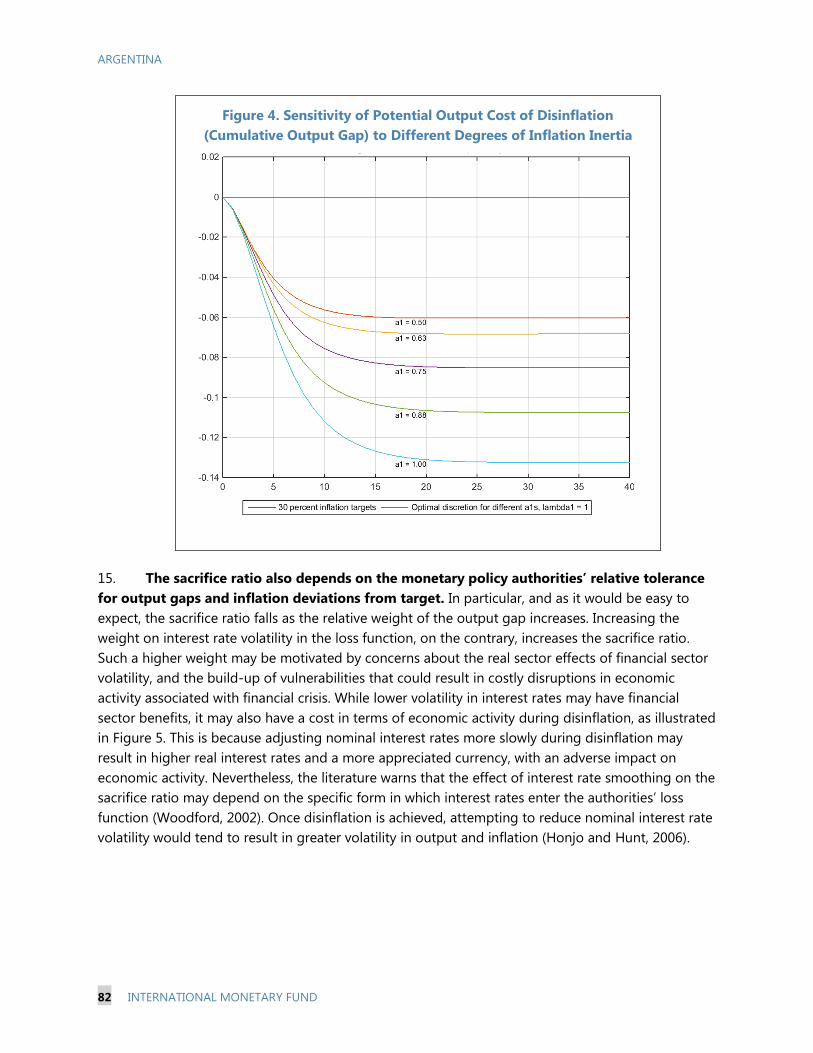
ARGENTINA


Figure 4. Sensitivity of Potential Output Cost of Disinflation

(Cumulative Output Gap) to Different Degrees of Inflation Inertia

15. The sacrifice ratio also depends on the monetary policy authorities’ relative tolerance

for output gaps and inflation deviations from target. In particular, and as it would be easy to

expect, the sacrifice ratio falls as the relative weight of the output gap increases. Increasing the

weight on interest rate volatility in the loss function, on the contrary, increases the sacrifice ratio.

Such a higher weight may be motivated by concerns about the real sector effects of financial sector

volatility, and the build-up of vulnerabilities that could result in costly disruptions in economic

activity associated with financial crisis. While lower volatility in interest rates may have financial

sector benefits, it may also have a cost in terms of economic activity during disinflation, as illustrated

in Figure 5. This is because adjusting nominal interest rates more slowly during disinflation may

result in higher real interest rates and a more appreciated currency, with an adverse impact on

economic activity. Nevertheless, the literature warns that the effect of interest rate smoothing on the

sacrifice ratio may depend on the specific form in which interest rates enter the authorities’ loss

function (Woodford, 2002). Once disinflation is achieved, attempting to reduce nominal interest rate

volatility would tend to result in greater volatility in output and inflation (Honjo and Hunt, 2006).

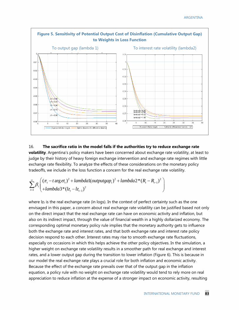
ARGENTINA


Figure 5. Sensitivity of Potential Output Cost of Disinflation (Cumulative Output Gap)

to Weights in Loss Function

To output gap (lambda 1) To interest rate volatility (lambda2)

16. The sacrifice ratio in the model falls if the authorities try to reduce exchange rate

volatility. Argentina’s policy makers have been concerned about exchange rate volatility, at least to

judge by their history of heavy foreign exchange intervention and exchange rate regimes with little

exchange rate flexibility. To analyze the effects of these considerations on the monetary policy

tradeoffs, we include in the loss function a concern for the real exchange rate volatility.

where lzt is the real exchange rate (in logs). In the context of perfect certainty such as the one

envisaged in this paper, a concern about real exchange rate volatility can be justified based not only

on the direct impact that the real exchange rate can have on economic activity and inflation, but

also on its indirect impact, through the value of financial wealth in a highly dollarized economy. The

corresponding optimal monetary policy rule implies that the monetary authority gets to influence

both the exchange rate and interest rates, and that both exchange rate and interest rate policy

decision respond to each other. Interest rates may rise to smooth exchange rate fluctuations,

especially on occasions in which this helps achieve the other policy objectives. In the simulation, a

higher weight on exchange rate volatility results in a smoother path for real exchange and interest

rates, and a lower output gap during the transition to lower inflation (Figure 6). This is because in

our model the real exchange rate plays a crucial role for both inflation and economic activity.

Because the effect of the exchange rate prevails over that of the output gap in the inflation

equation, a policy rule with no weight on exchange rate volatility would tend to rely more on real

appreciation to reduce inflation at the expense of a stronger impact on economic activity, resulting

2 2 2

1

21 1

( arg ) 1( ) 2*( )

3*( )

t t t t t

t

t t t

t et lambda outputgap lambda R R

lambda lz lz

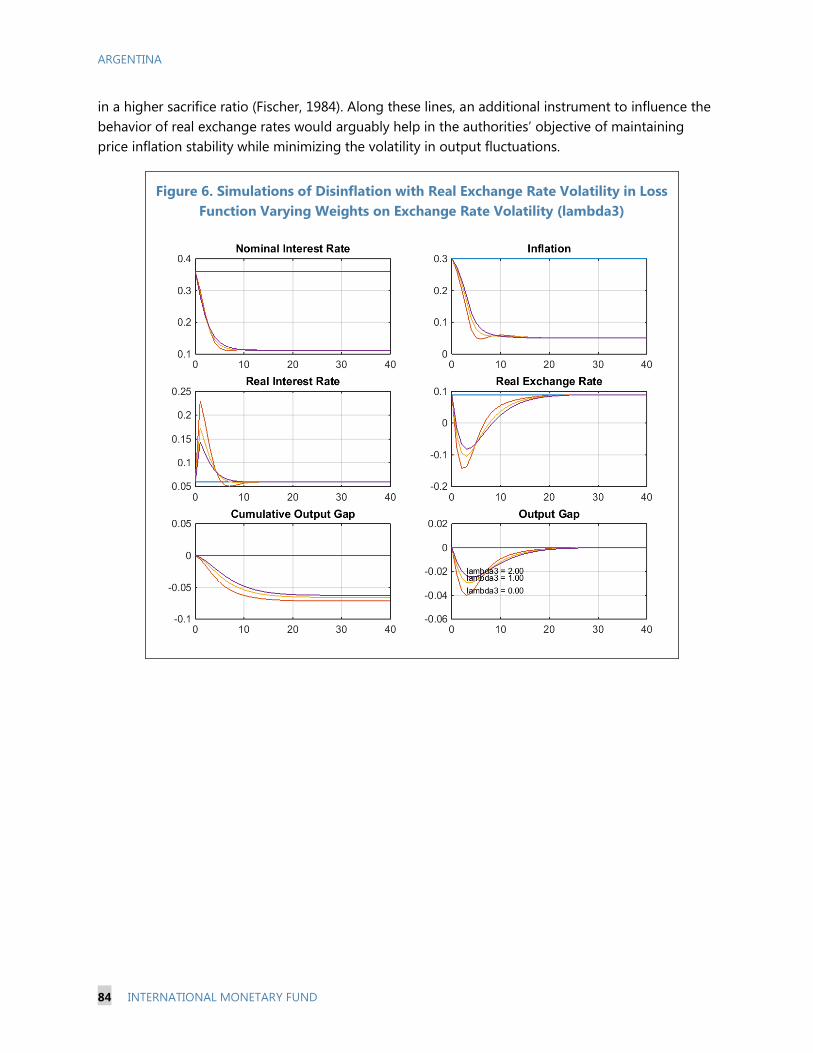
ARGENTINA


in a higher sacrifice ratio (Fischer, 1984). Along these lines, an additional instrument to influence the

behavior of real exchange rates would arguably help in the authorities’ objective of maintaining

price inflation stability while minimizing the volatility in output fluctuations.

Figure 6. Simulations of Disinflation with Real Exchange Rate Volatility in Loss

Function Varying Weights on Exchange Rate Volatility (lambda3)

ARGENTINA


References

Alichi, Ali, Kevin Clinton, Jihad Dagher, Ondra Kamenik, Douglas Laxton, and Marshall Mills, 2009, “A

Model for Full-Fledged Inflation Targeting and Application to Ghana,” IMF Working Paper

No. WP/10/25 (Washington, DC.: International Monetary Fund).

Alichi, Ali, Huigang Chen, Kevin Clinton, Charles Freedman, Marianne Johnson, Ondra Kamenik,

Turgut Kışınbay, and Douglas Laxton, 2009, “Inflation Targeting Under Imperfect Policy

Credibility, IMF Working Paper No. 09/94 (Washington, DC.: International Monetary Fund).

Amisano, Gianni and Gabriel Fagan, 2013, “Money growth and inflation: A regime switching

approach,” Journal of International Money and Finance 33 (2013) 118–145.

Argov, Eyal, Natan Epstein, Philippe Karam, Douglas Laxton, and David Rose, 2007, “Endogenous

Monetary Policy Credibility in a Small Macro Model of Israel,” IMF Working Paper No. 07/207

(Washington, DC.: International Monetary Fund).

Andrle, Michal, Andrew Berg, Enrico Berkes, Rafael A Portillo, Jan Vlcek, and R. Armando Morales,

2013, “Money Targeting in a Modern Forecasting and Policy Analysis System: An Application

to Kenya,” IMF Working Paper No. 13/239 (Washington, DC.: International Monetary Fund).

Aguirre, Horacio, Tamara Burdisso, and Federico Grillo, 2006, “Hacia una Estimación de la Demanda

de Dinero con Fines de Pronóstico: Argentina, 1993–2005,” Banco Central de la República

Argentina (BCRA) Estudio 45.

Aguirre, Horacio and Tamara Burdisso, 2008. "Dangerous Liaisons? An Empirical Assessment of

Inflation Targeting and Exchange Rate Regimes," BCRA Working Paper Series 200839,

Central Bank of Argentina, Economic Research Department, electronically available at

https://ideas.repec.org/p/bcr/wpaper/200839.html.

Ahrens, Steffen and Stephen Sacht, 2011, “Estimating a High-Frequency New-Keynesian Phillips

Curve, Kiel Working Paper No. 1686.

Albanesi, Stefania, 2007, “Inflation and Inequality,” Journal of Monetary Economics., Volume 54, pp

1088–1114.

Anderson, Palle, and William Wascher (1999), ‘Sacrifice Ratios and the Conduct of Monetary Policy in

Conditions of Low Inflation’, Bank of International Settlements Working Paper No. 82.

Banco Central de la República Argentina, 2016, Informe de Política Monetaria (Mayo).

Ball, Laurence, 1994, “What Determines the Sacrifice Ratio?” in Monetary Policy, The University of

Chicago Press, pp. 155–193.

Basco Emiliano, Laura D’Amato, and Lorena Garegnani, 2009, “Understanding the money–prices

relationship under low and high inflation regimes: Argentina 1977–2006,” Journal of

International Money and Finance 28 (2009) 1182–1203.

ARGENTINA


Basco Laura, Emiliano, Laura D’Amato, and Lorena Garegnani, 2012, “The information value of

money for forecasting purpose: The cases of Argentina and Chile,” Banco Central de la

República Argentina (October).

Benes, Jaromir, Marta Castello Branco, and David Vavra, 2007, “A Simple DGE Model for Inflation

Targeting,” IMF Working Paper No. 07/197 (Washington, DC.: International Monetary Fund).

Benes, Jaromir, 2014, “Simulate Disinflation in Optimal Policy Models,” unpublished mimeo.

Berg, A., P. Karam, and D. Laxton, 2006a, “A Practical Model-Based Approach to Monetary Policy

Analysis—Overview,” IMF Working Paper 06/080 (April 2006) (Washington, DC.: International

Monetary Fund).

———, 2006b, “Practical Model-Based Monetary Policy Analysis—A How-to Guide,” IMF Working

Paper 06/081 (April 2006) (Washington, DC.: International Monetary Fund).

Berg, A., Ostry, J.D., Zettelmeyer, J., 2008. What makes growth sustained? Working Paper 08/59,

March, International Monetary Fund, Washington, DC.

Blanchard, Olivier, 1998, “Optimal Speed of Disinflation: Hungary”, In Moderate inflation: the

experience of transition economies: proceedings of a seminar held in Budapest, Hungary, on

June 3, 1997. Washington, DC: International Monetary Fund, ISBN 1557756996. 1998,

p. 132–146 (Chapter 3).

Buiter, Willem H. and Clemens Graffe, 2001, “No Pain, No Gain? The Simple Analytics of Efficient

Disinflation in Open Economies,” European Bank for Reconstruction and Development.

Caldi, Fernando Gabriel, 2011, “Una Estimación de la Curva de Phillips para Argentina de 1974 a

2010: análisis de múltiples quiebres estructurales” Universidad de San Andres, electronically

available at http://repositorio.udesa.edu.ar/jspui/handle/10908/776.

Canales Kriljenko, Jorge Iván, Charles Freedman, Roberto Garcia-Saltos, Marianne Johnson, and

Douglas Laxton, 2009, “Adding Latin America to the Global Projection Model, IMF Working

Paper No. 09/85 (Washington, DC.: International Monetary Fund).

Carabenciov, I., I. Ermolaev, C. Freedman, M. Juillard, O. Kamenik, D. Korsunmov, and D. Laxton, 2008,

“A Small Multi-Country Global Projection Model,” IMF Working Paper No. 08/279

(Washington, DC.: International Monetary Fund).

Cardoso, Eliana, 1992, “Inflation and Poverty,” NBER Working Paper No. 4006.

Cavallo, A. (2012), Online and Official Price Indexes: Measuring Argentina’s Inflation, MIT Sloan,

Working Paper.

Celasun, Oya, R. Gaston Gelos, and Alessandro Prati, 2004, “Obstacles to Disinflation: What Is the

Role of Fiscal Expectations?,” IMF Working Paper No. 04/111 (Washington, DC.: International

Monetary Fund).

ARGENTINA


Coats, W., D. Laxton and D. Rose, 2003, The Czech National Bank’s Forecasting and Policy Analysis

System, (Prague, Czech Republic: Czech National Bank).

D´Amato, Laura and María Lorena Garegnani, 2009, “Studying the Short-Run Dynamics of Inflation:

Estimating a Hybrid New-Keynesian Phillips Curve for Argentina (1993–2007),” BCRA

Working Paper 2009 | 40.

D’Amato, L., Garegnani, M.L. and Sotes Paladino, J.M. (2007), Inflation Persistence and Changes in

the Monetary Regime: The Argentine Case, Working Paper 2007|23, Banco Central de la

República Argentina.

Dizioli, Allan and Jochen M. Schmittmann, 2015, “A Macro-Model Approach to Monetary Policy

Analysis and Forecasting for Vietnam,” IMF Working Paper No. 15/273 (Washington, DC.:

International Monetary Fund).

Elosegui, Pedro, Guillermo Escudé, Lorena Garegnani, and Juan Martín Sotes Paladino, 2007, “A

Small Economic Model for Argentina,” BCRA Paper Series No. 3 (February).

Escudé, G.J. (2007), ARGEM: A DSGE Model with Banks and Monetary Policy Regimes with two

Feedback Rules, Calibrated for Argentina, Working Paper 2007|21, Banco Central de la


Escudé, G.J. (2009), ARGEMmy: An Intermediate DSGE Calibrated/Estimated for Argentina: Two

Policy Rules are Often Better than One, Working Paper 2009|42, Banco Central de la


Fischer, Stanley, 1984, Real Balances, The Exchange Rate and Indexation: Real Variables In

Disinflation, The Quarterly Journal of Economics (1988) 103 (1): 27–49

Friedman, Benjamin M. (1994), ‘Comment on ‘‘What Determines the Sacrifice Ratio?’’ in N. G. Mankiw

(ed.), Monetary Policy. Chicago, IL: University of Chicago Press, 182–88.

Glüzmanna, Pablo Alfredo, Eduardo Levy-Yeyati and Federico Sturzenegger, 2012, “Exchange rate

undervaluation and economic growth: Díaz Alejandro (1965) revisited,” Economics Letters

117 (2012) 666–672.

Grigoli, Francesco, Alexander Herman, and Klaus Schmidt-Hebbel, 2014, “World Saving,” IMF

Working Paper WP/14/204.

Honjo, Keiko and Benjamin Hunt, 2006, “Stabilizing Inflation in Iceland,” IMF Working Paper No.

WP/06/262 (Washington, DC.: International Monetary Fund).

International Monetary Fund, 2016, “Exchange Rate Pass-Through in Latin America,” in Regional

Economic Outlook, Managing Transitions and Risks (April).

ARGENTINA


Isard, Peter, Douglas Laxton, Ann-Charlotte Eliasson, 2001, “Inflation Targeting with NAIRU

Uncertainty and Endogenous Policy Credibility,” IMF Working Paper No. 01/7 (Washington,

DC.: International Monetary Fund).

Jacome, Luis I., forthcoming, “The Road to Inflation Targeting in Argentina,” Selected Issues Paper

for the 2016 Article IV Consultation with Argentina.

Laxton, Douglas, David Rose, and Alasdair Scott, 2009, “Developing a Structured Forecasting and

Policy Analysis System to Support Inflation-Forecast Targeting (IFT),” IMF Working Paper No.

09/65 (Washington, DC.: International Monetary Fund).

Loayza, Norman and Romain Ranciere, 2006, Journal of Money, Credit and Banking, Vol 38, Issue 4,

pp. 1051–1076.

Moriyama, Kenji, 2011, “Inflation Inertia in Egypt and its Policy Implications,” IMF Working Paper No.

11/160 (Washington, DC.: International Monetary Fund).

Pescatori, Andrea and Jarkko Turunen, 2015, “Lower for Longer: Neutral Rates in the United States,”

IMF Working Paper No. 15/ 135 (Washington, DC.: International Monetary Fund).

Portillo, Rafael and Yulia Ustyugova, 2015, “A Model for Monetary Policy Analysis in Uruguay,” IMF

Working Paper No. 15/170 (Washington, DC.: International Monetary Fund).

Rodríguez Chatruc, Marisol, 2007, “La demanda de dinero en una economía abierta: el caso de

Argentina 1993–2006,” BCRA Documentos de Trabajo 2007 | 28.

Sánchez, Oscar, Juan Seade and Alejandro Werner, 1999, “Los Costos Asociados Al Proceso

Desinflacionario,” Banco de Mexico, Documento de Investigación No. 9903 (May).

Soldano Deheza, Juan Carlos N., 2005, Argentina y el Inflation Targeting. ¿Es posible su

implementación? Algunas consideraciones provenientes de la experiencia brasileña,

electronically available at http://econpapers.repec.org/paper/wpawuwpma/0505003.htm.

Tanner, Evan, forthcoming, “Disinflation, External Vulnerability, and Fiscal Intransigence: Some

Unpleasant Mundellian Arithmetic,” IMF Working Paper (Washington, DC.: International

Monetary Fund).

Woodford, Michael, 2003, “Optimal Interest-Rate Smoothing,” Review of Economic Studies (2003)

70 (4): 861–886.

Zhang, Lawrence, 2005. “Sacrifice Ratios with Long-Lived Effects,” International Finance 8:2, 2005: pp.

231–262.

http://econpapers.repec.org/paper/wpawuwpma/0505003.htm

ARGENTINA


Annex I. The Model

A. Phillips Curve

The Phillips curve captures the short-term tradeoff between economic activity and inflation. When

economic activity exceeds potential GDP, that is when the output gap ( _ tlgdp gap ) is positive, it

exerts inflationary pressure. The opposite is true when economic activity is below potential. But the

curve also recognizes that inflation typically has significant inertia, and only partially reflects

expectations of future inflation. The Phillips-type curve in this model also captures the fact that real

exchange rate movements ( zo

t ) have an impact on inflation in the form of a positive pass through.

Finally, supply shocks can also influence the evolution of consumer prices independently of demand

considerations, exchange rate pass through, or inflation dynamics ( ).1

B. Dynamic IS Equation

The dynamic IS equation captures the relationship between economic activity and monetary

conditions as well as spillovers from trading partners. Higher real interest rates ( _ trr gap ) lower

economic activity while more depreciated currencies in real terms ( _ tlz gap ) tend to boost it. Real

interest and exchange rates are measured relative to their equilibrium, time-varying levels. In

addition, the equation encompasses the view that economic activity in trading partners have a direct

impact on domestic economic activity through the foreign output gap ( _ _ tlx gdp gap ), after

recognizing that trading partners may have different long-term growth rates associated to among

other things different demographic structures and dynamics. The dynamic IS equation reckons

economic activity tends to move gradually and has a nontrivial backward looking component.

Finally, the error term includes demand shocks (independent from monetary conditions, inertia, and

foreign economic developments) that have an impact on economic activity. Autonomous fiscal

developments would appear as shocks to domestic demand.

1 2 3_ b * _ b * _ b * _

4* _ _ _ _

t l t t t

t t

lgdp gap lgdp gap rr gap lz gap

b lx gdp gap lgdp gap

C. Uncovered Interest Rate Parity and Exchange Rates

The model includes an uncovered interest rate parity equation expressed in real terms. It states that

real interest rate differentials tend to be associated to changes in the real exchange rate in the long

1 In all that follows, l before the variables means the variable is in natural logarithm, while the dot means the variable

is in log-difference. The dot4 means log difference four quarters apart. Nominal interest rates (R) represent the

natural logarithm of gross interest rates, for example, ln(1+R/100).

o

tcpi

1 1 2 31 1 a * 1 * a * _ z

o o o o o

ttt t t tcpi cpi a cpi lgdp gap a cpi

ARGENTINA


run, although short-term deviations (shocks) do take place. The real interest rate differentials are

relative to each country’s equilibrium real interest rate levels.

- rr (1-e)* - e R R / 4 _ ;e

t xt t t xt trr lz lz lz

The model allows expectations of the real exchange rate to have a backward and a forward looking

component. A sovereign spread is added to the version after estimation, to recognize the sharp

relaxation in financial repression.

1 1 = 1-e

t tlz lz lz

Nominal and real exchange rates are linked by the following identity:

1 1ls - cpi + cpit t t tlz l x l

D. Policy Reaction Function

The model includes a policy reaction function to set nominal interest rates. The equation is a crucial

element going forward as it would guide the central bank in setting its operational variable.

Nevertheless, it could be a controversial element for the estimation part because clearly Argentina

did not explicitly target inflation or use interest rates to achieve that objective. The analysis will later

include different policy reaction function, including by highlighting the policy frontier that depends

on weights to a loss function in terms of inflation and economic activity.

The policy reaction function standard in FPAS-type models implicitly argues that to stabilize inflation

to a given target, without undue disruptions in economic activity or financial distress, the central

bank should set nominal interest rates (Rt) around a neutral level associated with the prevailing real

interest rate ( trr ) and forward looking inflation (4

4

o

tcpi

), but should increase them when the forward

looking inflation exceeds the target or economic activity is above potential, that is if the output gap

( _ tlgdp gap ) is positive. It also suggests that to avoid financial distress, the nominal interest rates

should not be changed too frequently and would therefore display some inertia. In other words, the

policy reaction function could take the following form:

1 1 1

4 4

2 344 4...

g * 1 *...

+ g * g * _ _ ;

t t

o o

t t tt t t

R R g

rr cpi cpi target lgdp gap rn

E. Money Market

Given the importance of the need for seigniorage to explain the relatively high level of inflation

prevailing over the last decade, the model includes equations describing the behavior of monetary

aggregates. Money has been included in GPM-type models in the cases of Kenya (Andrle and

ARGENTINA


others, 2013) and Uruguay (Portillo and Ustyugova, 2015). For Argentina, Basco, D’Amato, and

Garegagni (2011) find that the introduction of the real money gap does not improve forecast

accuracy for quarterly data, but it significantly adds predictive power at lower frequencies.

Following Portillo and Ustyugova (2015), the model in this paper includes an error correction

specification for the evolution of the money aggregate M2. Changes in real money balances

( 2 cpio o

t tM ) are related to changes in economic activity lg

o

tdp and interest rates tR . In addition,

real money balances can vary to gradually adjust toward a long-run relationship akin to a money

demand equation ( 1tmondem ) and may also reflect changes linked to movements in the velocity of

money or shocks to the demand for money (o

v ).

where

l 2 5*lg 6* t t t t t tmondem M lcpi dp R v

Shocks to money demand can be persistent and add a trend to the level of real money balances.

1 12 cpi 1* 2* 4* _g 2o o o

t tt t tt

o

tM R R v mondemp Md

1 (1 )* _v _o o

t v t v tv v ss v

ARGENTINA


ENHANCING THE EFFECTIVENESS OF INFLATION

TARGETING IN ARGENTINA1

This note identifies key reforms to strengthen the effectiveness of inflation targeting in Argentina. The

Central Bank of the Republic of Argentina (BCRA) launched inflation targeting in September 2016, with

the objective of reducing inflation to 5 percent in 2019. The reforms involve strengthening the

institutional underpinnings of monetary policy and adjusting its policy and operational framework.

A. Introduction

1. Inflation in Argentina has been chronic throughout most of its modern history. By the

1950s, Argentina already featured two-digit inflation and, from 1975 onward, it accelerated and

reached three-digit rates. To cope with persistent inflation, successive stabilization plans—of a

variety of nature—were put in place, but most of them eventually failed. Thus, inflation hit a record

high of more than 3,000 percent by the late 1980s (see Box 1). The Convertibility Plan introduced in

the early 1990s, which had a currency board arrangement (CBA) as anchor, defeated inflation.

However, price stability lasted only a decade as the CBA was abandoned in the midst of a financial

crisis and inflation re-emerged as a result of expansionary fiscal and monetary policies.

2. The BCRA formally adopted inflation targeting in September 2016. The BCRA confirmed

the path of disinflation established at the beginning of the year, which aims at achieving 5 percent,

with a tolerance band of +/- 150 bps, in 2019—the inflation targets for 2017 and 2018 were ratified

at 12–17 percent and 8–12 percent, respectively. The BCRA also announced the adoption of a 7-day

repo rate as a policy rate, that will substitute todays’ 35-day Lebac rate. Policy decisions will be taken

by a new Monetary Policy Council.

3. This note identifies key reforms to enhance the effectiveness of inflation targeting in

Argentina. These reforms involve strengthening the institutional underpinnings of monetary policy

and adjusting its policy and operational framework. The rest of this paper is organized as follows:

Section B characterizes the transition to inflation targeting in Argentina and argues that the targets

set for disinflation seem to be ambitious; Section C highlights key institutional reforms that may

help to shift expectations forward; Section D identifies changes in the policy and operational

framework to enhance the effectiveness of inflation targeting.

1 Prepared by Luis Jacome.

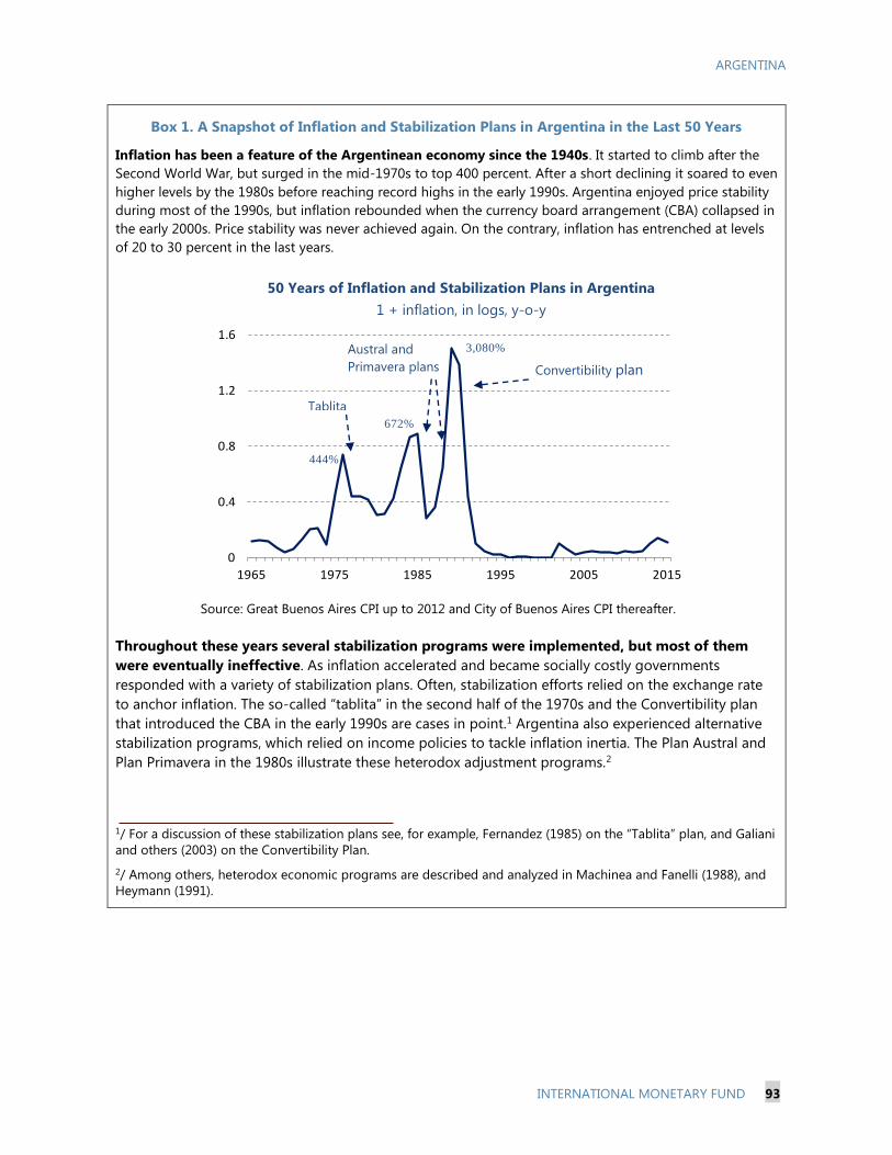
ARGENTINA


Box 1. A Snapshot of Inflation and Stabilization Plans in Argentina in the Last 50 Years

Inflation has been a feature of the Argentinean economy since the 1940s. It started to climb after the

Second World War, but surged in the mid-1970s to top 400 percent. After a short declining it soared to even

higher levels by the 1980s before reaching record highs in the early 1990s. Argentina enjoyed price stability

during most of the 1990s, but inflation rebounded when the currency board arrangement (CBA) collapsed in

the early 2000s. Price stability was never achieved again. On the contrary, inflation has entrenched at levels

of 20 to 30 percent in the last years.

Source: Great Buenos Aires CPI up to 2012 and City of Buenos Aires CPI thereafter.

Throughout these years several stabilization programs were implemented, but most of them

were eventually ineffective. As inflation accelerated and became socially costly governments

responded with a variety of stabilization plans. Often, stabilization efforts relied on the exchange rate

to anchor inflation. The so-called “tablita” in the second half of the 1970s and the Convertibility plan

that introduced the CBA in the early 1990s are cases in point.1 Argentina also experienced alternative

stabilization programs, which relied on income policies to tackle inflation inertia. The Plan Austral and

Plan Primavera in the 1980s illustrate these heterodox adjustment programs.2

1/ For a discussion of these stabilization plans see, for example, Fernandez (1985) on the “Tablita” plan, and Galiani

and others (2003) on the Convertibility Plan.

2/ Among others, heterodox economic programs are described and analyzed in Machinea and Fanelli (1988), and

Heymann (1991).

0

0.4

0.8

1.2

1.6

1965 1975 1985 1995 2005 2015

3,080%

444%

672%

50 Years of Inflation and Stabilization Plans in Argentina

1 + inflation, in logs, y-o-y

Tablita

Austral and

Primavera plans Convertibility plan

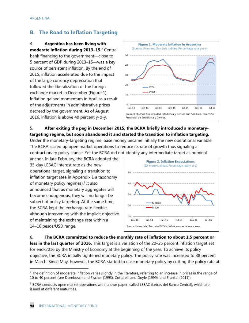
ARGENTINA


B. The Road to Inflation Targeting

4. Argentina has been living with

moderate inflation during 2013–15.2 Central

bank financing to the government—close to

5 percent of GDP during 2013–15—was a key

source of persistent inflation. By the end of

2015, inflation accelerated due to the impact

of the large currency depreciation that

followed the liberalization of the foreign

exchange market in December (Figure 1).

Inflation gained momentum in April as a result

of the adjustments in administrative prices

decreed by the government. As of August

2016, inflation is above 40 percent y-o-y.

5. After exiting the peg in December 2015, the BCRA briefly introduced a monetary-

targeting regime, but soon abandoned it and started the transition to inflation targeting.

Under the monetary-targeting regime, base money became initially the new operational variable.

The BCRA scaled up open market operations to reduce its rate of growth thus signaling a

contractionary policy stance. Yet the BCRA did not identify any intermediate target as nominal

anchor. In late February, the BCRA adopted the

35-day LEBAC interest rate as the new

operational target, signaling a transition to

inflation target (see in Appendix 1 a taxonomy

of monetary policy regimes).3 It also

announced that as monetary aggregates will

become endogenous, they will no longer be

subject of policy targeting. At the same time,

the BCRA kept the exchange rate flexible,

although intervening with the implicit objective

of maintaining the exchange rate within a

14–16 pesos/USD range.

6. The BCRA committed to reduce the monthly rate of inflation to about 1.5 percent or

less in the last quarter of 2016. This target is a variation of the 20–25 percent inflation target set

for end-2016 by the Ministry of Economy at the beginning of the year. To achieve its policy

objective, the BCRA initially tightened monetary policy. The policy rate was increased to 38 percent

in March. Since May, however, the BCRA started to ease monetary policy by cutting the policy rate at

2 The definition of moderate inflation varies slightly in the literature, referring to an increase in prices in the range of

10 to 40 percent (see Dornbusch and Fischer (1993), Cottarelli and Doyle (1999), and Frankel (2011)).

3 BCRA conducts open market operations with its own paper, called LEBAC (Letras del Banco Central), which are

issued at different maturities.

0

10

20

30

40

50

Jul-13 Jan-14 Jul-14 Jan-15 Jul-15 Jan-16 Jul-16

IPCSL

IPCBA

Figure 1. Moderate Inflation in Argentina

(Buenos Aires and San Luis indices, Percentage rate y-o-y)

Sources: Buenos Aires Ciudad Estadística y Censos and San Luis- Dirección

Provincial de Estadística y Censos.

10

20

30

40

50

Jan-14 Jul-14 Jan-15 Jul-15 Jan-16 Jul-16

Median

Mean

Source: Universidad Torcuato Di Tella, Inflation expectations survey.

Figure 2. Inflation Expectations

(12-months ahead, Percentage rate y-o-y)

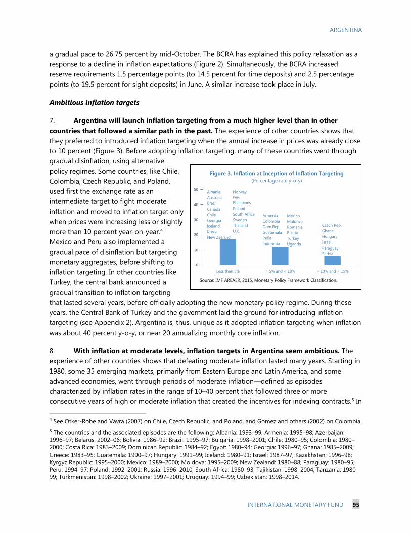
ARGENTINA


a gradual pace to 26.75 percent by mid-October. The BCRA has explained this policy relaxation as a

response to a decline in inflation expectations (Figure 2). Simultaneously, the BCRA increased

reserve requirements 1.5 percentage points (to 14.5 percent for time deposits) and 2.5 percentage

points (to 19.5 percent for sight deposits) in June. A similar increase took place in July.

Ambitious inflation targets

7. Argentina will launch inflation targeting from a much higher level than in other

countries that followed a similar path in the past. The experience of other countries shows that

they preferred to introduced inflation targeting when the annual increase in prices was already close

to 10 percent (Figure 3). Before adopting inflation targeting, many of these countries went through

gradual disinflation, using alternative

policy regimes. Some countries, like Chile,

Colombia, Czech Republic, and Poland,

used first the exchange rate as an

intermediate target to fight moderate

inflation and moved to inflation target only

when prices were increasing less or slightly

more than 10 percent year-on-year.4

Mexico and Peru also implemented a

gradual pace of disinflation but targeting

monetary aggregates, before shifting to

inflation targeting. In other countries like

Turkey, the central bank announced a

gradual transition to inflation targeting

that lasted several years, before officially adopting the new monetary policy regime. During these

years, the Central Bank of Turkey and the government laid the ground for introducing inflation

targeting (see Appendix 2). Argentina is, thus, unique as it adopted inflation targeting when inflation

was about 40 percent y-o-y, or near 20 annualizing monthly core inflation.

8. With inflation at moderate levels, inflation targets in Argentina seem ambitious. The

experience of other countries shows that defeating moderate inflation lasted many years. Starting in

1980, some 35 emerging markets, primarily from Eastern Europe and Latin America, and some

advanced economies, went through periods of moderate inflation—defined as episodes

characterized by inflation rates in the range of 10–40 percent that followed three or more

consecutive years of high or moderate inflation that created the incentives for indexing contracts.5 In

4 See Otker-Robe and Vavra (2007) on Chile, Czech Republic, and Poland, and Gómez and others (2002) on Colombia.

5 The countries and the associated episodes are the following: Albania: 1993–99; Armenia: 1995–98; Azerbaijan:

1996–97; Belarus: 2002–06; Bolivia: 1986–92; Brazil: 1995–97; Bulgaria: 1998–2001; Chile: 1980–95; Colombia: 1980–

2000; Costa Rica: 1983–2009; Dominican Republic: 1984–92; Egypt: 1980–94; Georgia: 1996–97; Ghana: 1985–2009;

Greece: 1983–95; Guatemala: 1990–97; Hungary: 1991–99; Iceland: 1980–91; Israel: 1987–97; Kazakhstan: 1996–98;

Kyrgyz Republic: 1995–2000; Mexico: 1989–2000; Moldova: 1995–2009; New Zealand: 1980–88; Paraguay: 1980–95;

Peru: 1994–97; Poland: 1992–2001; Russia: 1996–2010; South Africa: 1980–93; Tajikistan: 1998–2004; Tanzania: 1980–

99; Turkmenistan: 1998–2002; Ukraine: 1997–2001; Uruguay: 1994–99; Uzbekistan: 1998–2014.

0

10

20

30

40

50

Less than 5% > 5% and < 10% > 10% and < 15%

Albania

Australia

Brazil

Canada

Chile

Georgia

Iceland

Korea

New Zealand

Norway

Peru

Phillipines

Poland

South Africa

Sweden

Thailand

U.K.

Armenia

Colombia

Dom.Rep.

Guatemala

India

Indonesia

Czech Rep.

Ghana

Hungary

Israel

Paraguay

Serbia

Mexico

Moldova

Romania

Russia

Turkey

Uganda

Source: IMF AREAER, 2015, Monetary Policy Framework Classification.

Figure 3. Inflation at Inception of Inflation Targeting

(Percentage rate y-o-y)

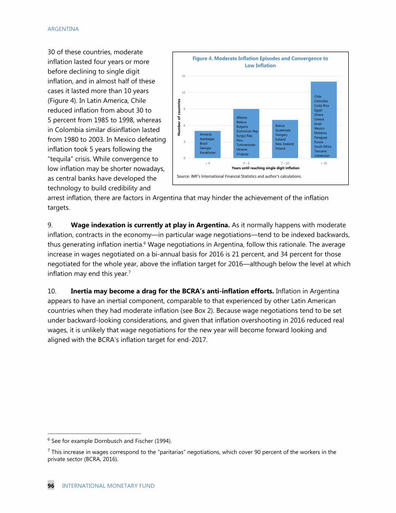
ARGENTINA


30 of these countries, moderate

inflation lasted four years or more

before declining to single digit

inflation, and in almost half of these

cases it lasted more than 10 years

(Figure 4). In Latin America, Chile

reduced inflation from about 30 to

5 percent from 1985 to 1998, whereas

in Colombia similar disinflation lasted

from 1980 to 2003. In Mexico defeating

inflation took 5 years following the

“tequila” crisis. While convergence to

low inflation may be shorter nowadays,

as central banks have developed the

technology to build credibility and

arrest inflation, there are factors in Argentina that may hinder the achievement of the inflation

targets.

9. Wage indexation is currently at play in Argentina. As it normally happens with moderate

inflation, contracts in the economy—in particular wage negotiations—tend to be indexed backwards,

thus generating inflation inertia.6 Wage negotiations in Argentina, follow this rationale. The average

increase in wages negotiated on a bi-annual basis for 2016 is 21 percent, and 34 percent for those

negotiated for the whole year, above the inflation target for 2016—although below the level at which

inflation may end this year.7

10. Inertia may become a drag for the BCRA’s anti-inflation efforts. Inflation in Argentina

appears to have an inertial component, comparable to that experienced by other Latin American

countries when they had moderate inflation (see Box 2). Because wage negotiations tend to be set

under backward-looking considerations, and given that inflation overshooting in 2016 reduced real

wages, it is unlikely that wage negotiations for the new year will become forward looking and

aligned with the BCRA’s inflation target for end-2017.

6 See for example Dornbusch and Fischer (1994).

7 This increase in wages correspond to the “paritarias” negotiations, which cover 90 percent of the workers in the

private sector (BCRA, 2016).

Source: IMF's International Financial Statistics and author's calculations.

0

3

6

9

12

15

< 4 4 - 6 7 - 10 > 10

Nu

mb

er

of

co

un

trie

s

Years until reaching single digit inflation

Armenia

Azerbaijan

Brazil

Georgia

Kazakhstan

Albania

Belarus

Bulgaria

Dominican Rep.

Kyrgyz Rep.

Peru

Turkmenistan

Ukraine

Uruguay

Bolivia

Guatemala

Hungary

Iceland

New Zealand

Poland

Chile

Colombia

Costa Rica

Egypt

Ghana

Greece

Israel

Mexico

Moldova

Paraguay

Russia

South Africa

Tanzania

Uzbekistan

Figure 4. Moderate Inflation Episodes and Convergence to

Low Inflation

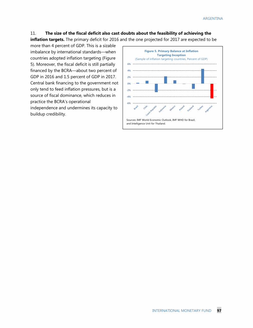
ARGENTINA


11. The size of the fiscal deficit also cast doubts about the feasibility of achieving the

inflation targets. The primary deficit for 2016 and the one projected for 2017 are expected to be

more than 4 percent of GDP. This is a sizable

imbalance by international standards—when

countries adopted inflation targeting (Figure

5). Moreover, the fiscal deficit is still partially

financed by the BCRA—about two percent of

GDP in 2016 and 1.5 percent of GDP in 2017.

Central bank financing to the government not

only tend to feed inflation pressures, but is a

source of fiscal dominance, which reduces in

practice the BCRA’s operational

independence and undermines its capacity to

buildup credibility.

Sources: IMF World Economic Outlook, IMF WHD for Brazil,

and Intelligence Unit for Thailand.

-6%

-4%

-2%

0%

2%

4%

6%

Figure 5. Primary Balance at Inflation

Targeting Inception

(Sample of inflation targeting countries, Percent of GDP)

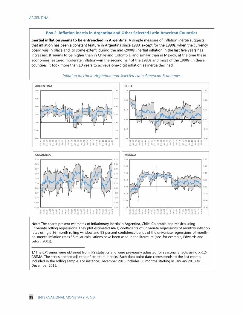
ARGENTINA


Box 2. Inflation Inertia in Argentina and Other Selected Latin American Countries

Inertial inflation seems to be entrenched in Argentina. A simple measure of inflation inertia suggests

that inflation has been a constant feature in Argentina since 1980, except for the 1990s, when the currency

board was in place and, to some extent. during the mid-2000s. Inertial inflation in the last five years has

increased. It seems to be higher than in Chile and Colombia, and similar than in Mexico, at the time these

economies featured moderate inflation—in the second half of the 1980s and most of the 1990s. In these

countries, it took more than 10 years to achieve one-digit inflation as inertia declined.

Inflation Inertia in Argentina and Selected Latin American Economies

Note: The charts present estimates of inflationary inertia in Argentina, Chile, Colombia and Mexico using

univariate rolling regressions. They plot estimated AR(1) coefficients of univariate regressions of monthly inflation

rates using a 36-month rolling window and 95 percent confidence bands of the univariate regressions of month-

on-month inflation rates.1 Similar calculations have been used in the literature (see, for example, Edwards and

Lefort, 2002).

1/ The CPI series were obtained from IFS statistics and were previously adjusted for seasonal effects using X-12-

ARIMA. The series are not adjusted of structural breaks. Each data point date corresponds to the last month

included in the rolling sample. For instance, December 2015 includes 36 months starting in January 2013 to

December 2015.

-1.00

-0.50

0.00

0.50

1.00

1.50

2.00

-1.00

-0.50

0.00

0.50

1.00

1.50

2.00

Dec-

81

Jun

-83

Dec-

84

Jun

-86

Dec-

87

Jun

-89

Dec-

90

Jun

-92

Dec-

93

Jun

-95

Dec-

96

Jun

-98

Dec-

99

Jun

-01

Dec-

02

Jun

-04

Dec-

05

Jun

-07

Dec-

08

Jun

-10

Dec-

11

Jun

-13

Dec-

14

Jun

-16

ARGENTINA

-0.80

-0.60

-0.40

-0.20

0.00

0.20

0.40

0.60

0.80

1.00

1.20

-0.80

-0.60

-0.40

-0.20

0.00

0.20

0.40

0.60

0.80

1.00

1.20

Dec-

81

Jun

-83

Dec-

84

Jun

-86

Dec-

87

Jun

-89

Dec-

90

Jun

-92

Dec-

93

Jun

-95

Dec-

96

Jun

-98

Dec-

99

Jun

-01

Dec-

02

Jun

-04

Dec-

05

Jun

-07

Dec-

08

Jun

-10

Dec-

11

Jun

-13

Dec-

14

Jun

-16

COLOMBIA

-1.00

-0.50

0.00

0.50

1.00

1.50

-1.00

-0.50

0.00

0.50

1.00

1.50

Dec-

81

Jun

-83

Dec-

84

Jun

-86

Dec-

87

Jun

-89

Dec-

90

Jun

-92

Dec-

93

Jun

-95

Dec-

96

Jun

-98

Dec-

99

Jun

-01

Dec-

02

Jun

-04

Dec-

05

Jun

-07

Dec-

08

Jun

-10

Dec-

11

Jun

-13

Dec-

14

Jun

-16

CHILE

-1.50

-1.00

-0.50

0.00

0.50

1.00

1.50

2.00

-1.50

-1.00

-0.50

0.00

0.50

1.00

1.50

2.00

Dec-

81

Jun

-83

Dec-

84

Jun

-86

Dec-

87

Jun

-89

Dec-

90

Jun

-92

Dec-

93

Jun

-95

Dec-

96

Jun

-98

Dec-

99

Jun

-01

Dec-

02

Jun

-04

Dec-

05

Jun

-07

Dec-

08

Jun

-10

Dec-

11

Jun

-13

Dec-

14

Jun

-16

MEXICO

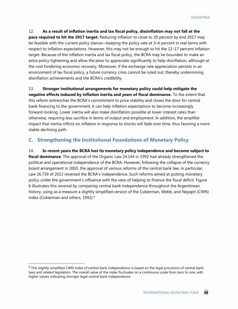
ARGENTINA


12. As a result of inflation inertia and lax fiscal policy, dissinflation may not fall at the

pace required to hit the 2017 target. Reducing inflation to close to 20 percent by end 2017 may

be feasible with the current policy stance—keeping the policy rate at 3–4 percent in real terms with

respect to inflation expectations. However, this may not be enough to hit the 12–17 percent inflation

target. Because of the inflation inertia and lax fiscal policy, the BCRA may be bounded to make an

extra policy tightening and allow the peso to appreciate significantly to help disinflation, although at

the cost hindering economic recovery. Moreover, if the exchange rate appreciation persists in an

environment of lax fiscal policy, a future currency crisis cannot be ruled out, thereby undermining

disinflation achievements and the BCRA’s credibility.

13. Stronger institutional arrangements for monetary policy could help mitigate the

negative effects induced by inflation inertia and years of fiscal dominance. To the extent that

this reform entrenches the BCRA’s commitment to price stability and closes the door for central

bank financing to the government, it can help inflation expectations to become increasingly

forward-looking. Lower inertia will also make disinflation possible at lower interest rates than

otherwise, requiring less sacrifice in terms of output and employment. In addition, the amplifier

impact that inertia inflicts on inflation in response to shocks will fade over time, thus favoring a more

stable declining path.

C. Strengthening the Institutional Foundations of Monetary Policy

14. In recent years the BCRA lost its monetary policy independence and become subject to

fiscal dominance. The approval of the Organic Law 24.144 in 1992 had already strengthened the

political and operational independence of the BCRA. However, following the collapse of the currency

board arrangement in 2003, the approval of various reforms of the central bank law, in particular,

Law 26.739 of 2012 reversed the BCRA’s independence. Such reforms aimed at putting monetary

policy under the government’s influence with the view of helping to finance the fiscal deficit. Figure

6 illustrates this reversal by comparing central bank independence throughout the Argentinean

history, using as a measure a slightly simplified version of the Cukierman, Webb, and Neyapti (CWN)

index (Cukierman and others, 1992).8

8 This slightly simplified CWN index of central bank independence is based on the legal provisions of central bank

laws and related legislation. The overall value of the index fluctuates on a continuous scale from zero to one, with

higher values indicating stronger legal central bank independence.

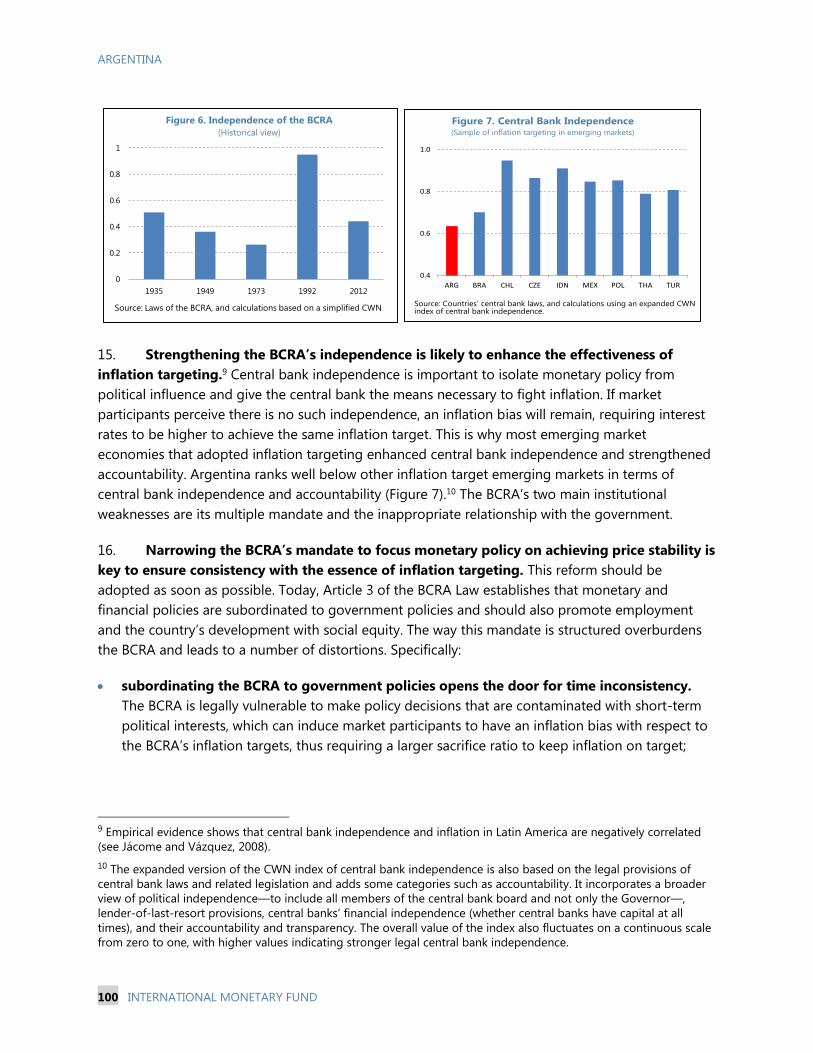
ARGENTINA


15. Strengthening the BCRA’s independence is likely to enhance the effectiveness of

inflation targeting.9 Central bank independence is important to isolate monetary policy from

political influence and give the central bank the means necessary to fight inflation. If market

participants perceive there is no such independence, an inflation bias will remain, requiring interest

rates to be higher to achieve the same inflation target. This is why most emerging market

economies that adopted inflation targeting enhanced central bank independence and strengthened

accountability. Argentina ranks well below other inflation target emerging markets in terms of

central bank independence and accountability (Figure 7).10 The BCRA’s two main institutional

weaknesses are its multiple mandate and the inappropriate relationship with the government.

16. Narrowing the BCRA’s mandate to focus monetary policy on achieving price stability is

key to ensure consistency with the essence of inflation targeting. This reform should be

adopted as soon as possible. Today, Article 3 of the BCRA Law establishes that monetary and

financial policies are subordinated to government policies and should also promote employment

and the country’s development with social equity. The way this mandate is structured overburdens

the BCRA and leads to a number of distortions. Specifically:

subordinating the BCRA to government policies opens the door for time inconsistency.

The BCRA is legally vulnerable to make policy decisions that are contaminated with short-term

political interests, which can induce market participants to have an inflation bias with respect to

the BCRA’s inflation targets, thus requiring a larger sacrifice ratio to keep inflation on target;

9 Empirical evidence shows that central bank independence and inflation in Latin America are negatively correlated

(see Jácome and Vázquez, 2008).

10 The expanded version of the CWN index of central bank independence is also based on the legal provisions of

central bank laws and related legislation and adds some categories such as accountability. It incorporates a broader

view of political independence—to include all members of the central bank board and not only the Governor—,

lender-of-last-resort provisions, central banks’ financial independence (whether central banks have capital at all

times), and their accountability and transparency. The overall value of the index also fluctuates on a continuous scale

from zero to one, with higher values indicating stronger legal central bank independence.

0

0.2

0.4

0.6

0.8

1

1935 1949 1973 1992 2012

Figure 6. Independence of the BCRA

(Historical view)

Source: Laws of the BCRA, and calculations based on a simplified CWN

0.4

0.6

0.8

1.0

ARG BRA CHL CZE IDN MEX POL THA TUR

Figure 7. Central Bank Independence(Sample of inflation targeting in emerging markets)

Source: Countries’ central bank laws, and calculations using an expanded CWN index of central bank independence.

ARGENTINA


promoting development and social equity does not respond directly to monetary policy.

Moreover, it can even be in conflict with the objective of price stability, thus making central bank

accountability difficult in practice.

monetary policy should not explicitly promote employment either. Unlike in advanced

economies, employment in emerging markets are vulnerable to terms of trade and political

development shocks. Thus, holding the BCRA responsible for creating employment risks

undermining monetary policy credibility and makes it difficult to hold the BCRA accountable.

17. The BCRA mandate should focus on its core functions. On monetary policy, the BCRA

should aim at preserving price stability while maintaining the objective of financial stability given

that it has banking regulation and supervision responsibilities.

18. To the extent possible, the central bank law should be amended to explicitly delink

monetary policy formulation from government policies. Governments are potentially more

interested in pursuing short-term goals—sometimes associated with electoral calendars, at the

expense of not preserving price stability. Article 3 in the 1992 Law illustrates how to phrase an

alternative text that grants political autonomy to the BCRA.

19. Eliminating fiscal dominance is critical to strengthen the operational independence of

the BCRA and build up credibility. While operational independence is typically about ensuring

that the central bank manages its short-term interest rate without government interference, in

Argentina it is mostly about restricting fiscal dominance under the form of central bank financing to

the government. Article 20 of the central bank law includes a number of provisions that render a

level of credit to the government—extended at a zero interest rate—that is large by international

standards. Thus, a legal reform is warranted to eliminate all forms of central bank financing to the

government. As a second best, the law could limit the sources of central bank financing to only

transitory advances up to 10 percent of government revenues in the previous 12 months—as set in

Article 20. However, this money should be paid back not later than in 180 days and charged a

market interest rate. All other forms of government financing established in this article should be

banned.11 Good practices to rule central bank financing to the government are summarized in Box 3.

As for the unrealized profits associated with currency depreciations, a legal reform is necessary to

prevent these funds from being transferred to the government. They should be kept on a reserve

account up to some relative level to be used whenever currency appreciations generate losses.

11 Article 20 authorizes the BCRA to extend: (i) transitory advances up to an amount equivalent to 12 percent of base

money; (ii) advances to the government up 10 percent of the government revenues in the last 12 months; and (iii)

additional transitory advances for up to 10 percent of the revenues in cash obtained by the government in the last

12 months.

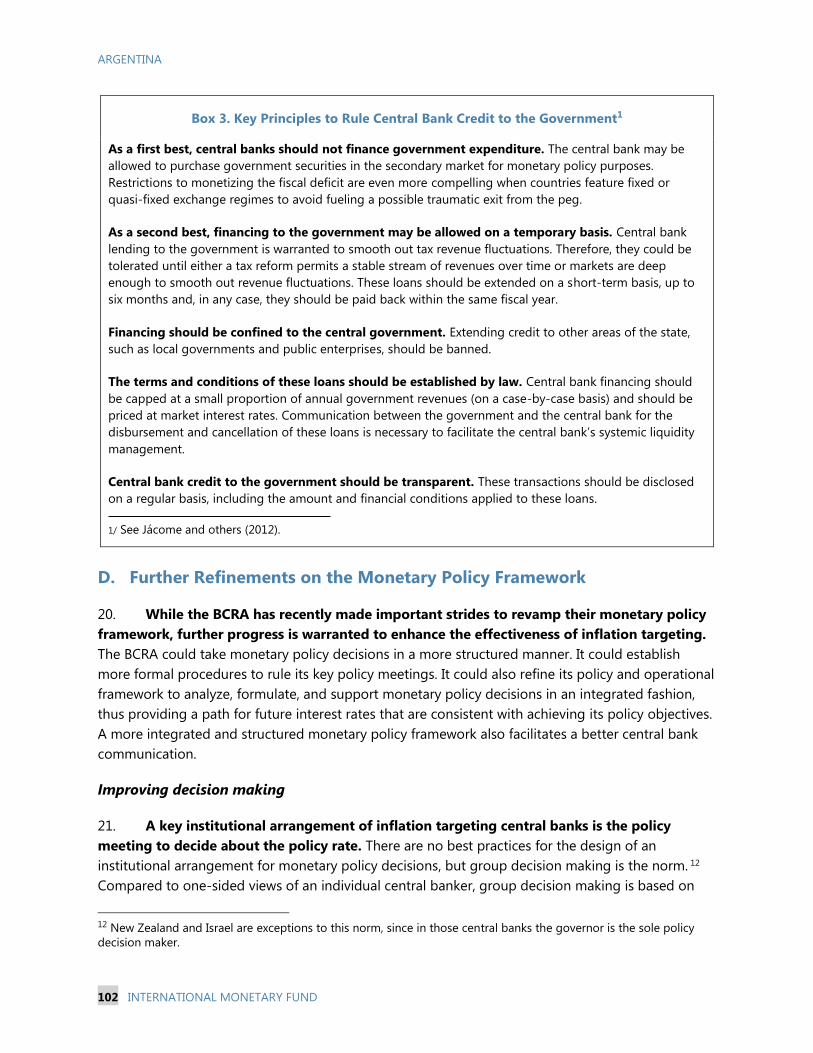
ARGENTINA


Box 3. Key Principles to Rule Central Bank Credit to the Government1

As a first best, central banks should not finance government expenditure. The central bank may be

allowed to purchase government securities in the secondary market for monetary policy purposes.

Restrictions to monetizing the fiscal deficit are even more compelling when countries feature fixed or

quasi-fixed exchange regimes to avoid fueling a possible traumatic exit from the peg.

As a second best, financing to the government may be allowed on a temporary basis. Central bank

lending to the government is warranted to smooth out tax revenue fluctuations. Therefore, they could be

tolerated until either a tax reform permits a stable stream of revenues over time or markets are deep

enough to smooth out revenue fluctuations. These loans should be extended on a short-term basis, up to

six months and, in any case, they should be paid back within the same fiscal year.

Financing should be confined to the central government. Extending credit to other areas of the state,

such as local governments and public enterprises, should be banned.

The terms and conditions of these loans should be established by law. Central bank financing should

be capped at a small proportion of annual government revenues (on a case-by-case basis) and should be

priced at market interest rates. Communication between the government and the central bank for the

disbursement and cancellation of these loans is necessary to facilitate the central bank’s systemic liquidity

management.

Central bank credit to the government should be transparent. These transactions should be disclosed

on a regular basis, including the amount and financial conditions applied to these loans.

1/ See Jácome and others (2012).

D. Further Refinements on the Monetary Policy Framework

20. While the BCRA has recently made important strides to revamp their monetary policy

framework, further progress is warranted to enhance the effectiveness of inflation targeting.

The BCRA could take monetary policy decisions in a more structured manner. It could establish

more formal procedures to rule its key policy meetings. It could also refine its policy and operational

framework to analyze, formulate, and support monetary policy decisions in an integrated fashion,

thus providing a path for future interest rates that are consistent with achieving its policy objectives.

A more integrated and structured monetary policy framework also facilitates a better central bank

communication.

Improving decision making

21. A key institutional arrangement of inflation targeting central banks is the policy

meeting to decide about the policy rate. There are no best practices for the design of an

institutional arrangement for monetary policy decisions, but group decision making is the norm. 12

Compared to one-sided views of an individual central banker, group decision making is based on

12 New Zealand and Israel are exceptions to this norm, since in those central banks the governor is the sole policy

decision maker.

ARGENTINA


diverse views, and is likely to produce better interpretation of information, data, and results from

considering alternative scenarios. In general, societies tend to be reluctant to delegate on a single

person the adoption of policy decisions—such as the level of interest rates that have direct

implications on inflation and economic activity—in institutions that enjoy political independence.

22. The BCRA could better structure policy decision making by either instituting a regular

policy meeting of its board or by creating a monetary policy committee (MPC). This

institutional arrangement will replace the current setup, where decisions on the policy rate are

informally discussed by an ad-hoc committee, and are legally taken by the BCRA governor. In either

arrangement, policy rate decisions would be the result of group decision making. There is no

standard international practice that favors either of these arrangements. An MPC exists in some

countries, while in others the central bank board is in charge of deciding about the policy rate (see

Table 1). 13 The latter is the prevailing arrangement in Latin America (Brazil, Chile, Colombia, Mexico,

Peru) as only in Guatemala an MPC exists. In the sample of inflation targeting countries in Table 1,

the central bank board plays the role of the MPC in most cases, the decision-making body is

comprised of 5 to 10 members and external members are appointed in some cases.14 No consensus

is required to take decisions, and the preannounced meetings take place either eight or 12 times in

the year, except in Australia and Mexico.

13 For an expanded discussion about why MPCs exist and how they work, see for example Blinder (2007).

14 The size and composition of the MPC, and how its members are selected, vary across countries. For a discussion,

see for example Berger and others (2006) and Vandenbussche (2006).

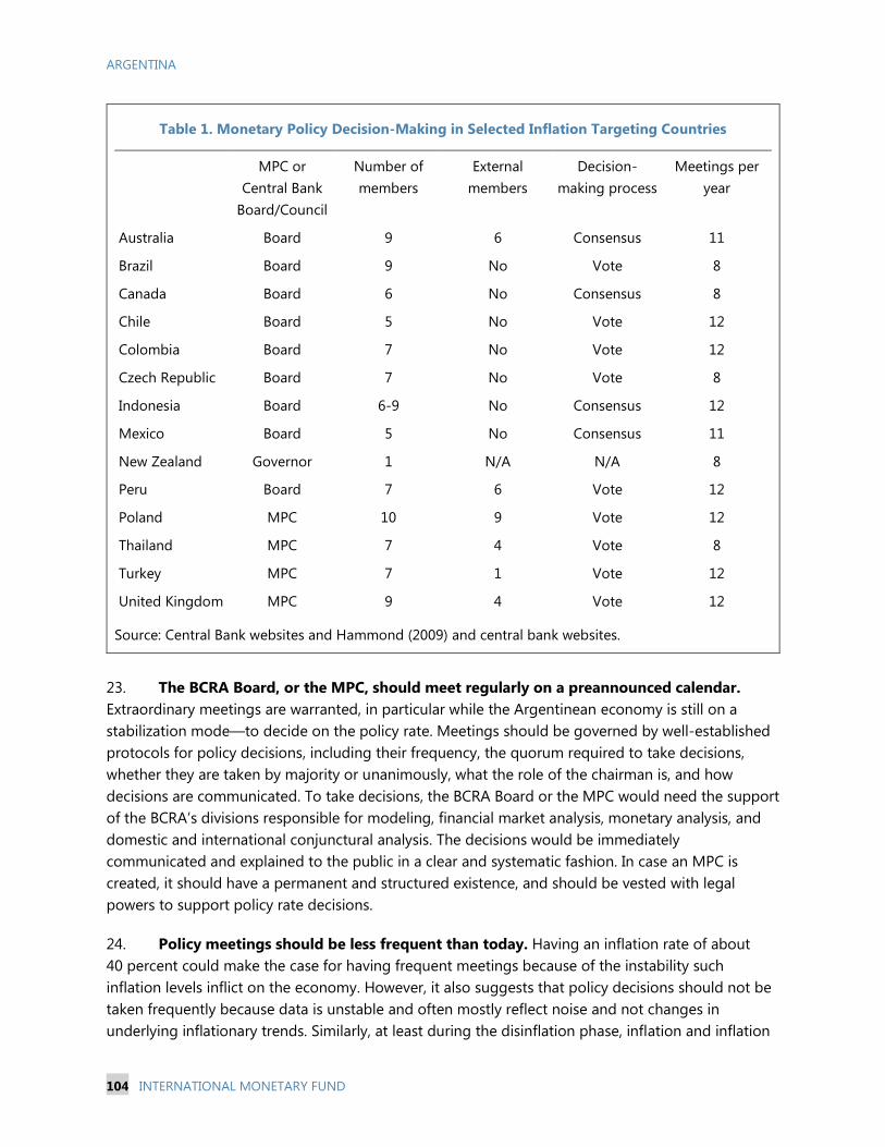
ARGENTINA


Table 1. Monetary Policy Decision-Making in Selected Inflation Targeting Countries

MPC or

Central Bank

Board/Council

Number of

members

External

members

Decision-

making process

Meetings per

year

Australia Board 9 6 Consensus 11

Brazil Board 9 No Vote 8

Canada Board 6 No Consensus 8

Chile Board 5 No Vote 12

Colombia Board 7 No Vote 12

Czech Republic Board 7 No Vote 8

Indonesia Board 6-9 No Consensus 12

Mexico Board 5 No Consensus 11

New Zealand Governor 1 N/A N/A 8

Peru Board 7 6 Vote 12

Poland MPC 10 9 Vote 12

Thailand MPC 7 4 Vote 8

Turkey MPC 7 1 Vote 12

United Kingdom MPC 9 4 Vote 12

Source: Central Bank websites and Hammond (2009) and central bank websites.

23. The BCRA Board, or the MPC, should meet regularly on a preannounced calendar.

Extraordinary meetings are warranted, in particular while the Argentinean economy is still on a

stabilization mode—to decide on the policy rate. Meetings should be governed by well-established

protocols for policy decisions, including their frequency, the quorum required to take decisions,

whether they are taken by majority or unanimously, what the role of the chairman is, and how

decisions are communicated. To take decisions, the BCRA Board or the MPC would need the support

of the BCRA’s divisions responsible for modeling, financial market analysis, monetary analysis, and

domestic and international conjunctural analysis. The decisions would be immediately

communicated and explained to the public in a clear and systematic fashion. In case an MPC is

created, it should have a permanent and structured existence, and should be vested with legal

powers to support policy rate decisions.

24. Policy meetings should be less frequent than today. Having an inflation rate of about

40 percent could make the case for having frequent meetings because of the instability such

inflation levels inflict on the economy. However, it also suggests that policy decisions should not be

taken frequently because data is unstable and often mostly reflect noise and not changes in

underlying inflationary trends. Similarly, at least during the disinflation phase, inflation and inflation

ARGENTINA


expectations may be volatile. The possible ill effects stemming from this second consideration

outweigh the likely benefits of the first.

The policy framework

25. Building a forecasting and policy analysis system is important to support the inflation

targeting regime.15 As a first step, the BCRA need to achieve a clear understanding of the

transmission mechanism of monetary policy. Building on this understanding, the policy framework

should consist of four interlinked blocks: (i) data monitoring and management; (ii) short-term

forecasting; (iii) medium-term forecasting; and (iv) reporting. The picture of a transmission

mechanism has to bring a solid idea about the way key variables react to monetary policy

instruments, as well as to other shocks affecting the economy.

26. Argentina needs to preserve and perfect the quality of inflation and output data. Since

the previous consumer price index (CPI) was widely manipulated, the new CPI may only gain

credibility overtime. At the beginning, negotiations of contracts, in particular of wage increases, may

be impaired by the lack of trust on the inflation data. Policymakers’ analysis would also suffer from

this deficiency as they face inconsistent data series and series that are not appropriately seasonally

adjusted. Similar problems arise from GDP data weaknesses because of the limitations they impose

for calculating the output gap.

27. The BCRA needs to refine some of its monetary operations. The BCRA may consider two

alternatives for the term of the policy rate—an overnight rate and a seven-day rate—and either

target a market rate or attach it to a central bank policy instrument.16 As a tentative proposal, the

BCRA could consider adopting a policy rate attached to a seven-day term deposit facility offered

two times per week, which would provide an effective policy signal and anchor to short-term

interest rates. The BCRA would also conduct ad hoc open market operations on any day when

overnight rates deviated materially from the policy rate. While building its expertise in liquidity

forecasting, the BCRA may rely on an interest rate corridor supported by standing facilities—deposit

and lending—that are narrow enough to limit interest rate volatility, but at the same time wide

enough to encourage interbank borrowing and lending.

28. A clear strategy is also needed to deal with structural liquidity. Market-based

instruments are preferred to fully support development of the financial markets. Initial focus should

be on 1-month, 3-month and perhaps 6-month maturities. The issuance method should change to

fixed-volume auctions, using a multiple price method of allocation.

15 This is a standard policy framework built by many central banks that adopted inflation targeting. Berg and others,

2006a and 2006b, provides a description of this framework and how it operates.

16 An expanded discussion about the pros and cons of these two alternatives and its operational aspects was

submitted to the BCRA authorities in August 2016.

ARGENTINA


Communication

29. The CBRA should continue enhancing gradually its communication, explaining policy

decisions largely based on forward-looking indicators. The BCRA cannot become immediately as

transparent as other inflation targeting central banks because it is still in the process of

understanding how monetary policy is transmitted to the real sector. However, it should explain how

monetary policy is formulated and implemented, highlighting potential downside risks for achieving

the inflation target. This involves making available and disseminating the information and data used

to take current policy decisions on a timely basis with emphasis on future or expected information. If

economic agents understand the goals pursued by the BCRA and the policy instruments used to

achieve such goals, the effectiveness of monetary policy is likely to increase. Enhancing

communication and transparency is also a matter of good governance, which becomes particularly

important should the BCRA is granted more political independence.

30. By explaining its policy decisions and targets and by delivering on those promises, the

BCRA would continue building credibility. The BCRA would need to act consistently with respect

to its reaction function. When central bank reactions are unpredictable or inconsistent, uncertainty

leads to market volatility because economic agents do not know what to expect. As a result, market

expectations about inflation may drift upwards from the central bank’s target, thus requiring an

extra tightening effort. Consistency between policy actions and communications is a necessary

condition to buildup credibility, which would reinforce the effectiveness of monetary policy.

31. Yet, communication should go beyond explaining the rationale for policy decisions

and stress that low and stable inflation is welfare improving. This should take the form of an

educational campaign that reaches the society at large, with the view of building up support for an

autonomous—from political pressures—and accountable BCRA. Reaching out the public at large is

important in Argentina given its recent history of central bank independence reversal. Such

initiatives will help the public understand the benefits of low and stable inflation toward fostering

broad-based economic growth, and the rationale for providing a central bank with an appropriate

degree of operational independence to carry out that mission. The BCRA can produce educational

materials to inform students about basic elements of monetary policy, including the role of money,

the concept of inflation, and the rationale for the anti-inflation mandate of the central bank. The

BCRA can also engage in active outreach to business associations, labor unions, and various other

types of community organizations.

ARGENTINA


References

Banco Central de la República Argentina (2016), “Informe de Política Monetaria (Julio).

Berg, Andrew, Philipe Karan, and Douglas Laxton (2006a), “A Practical Model Approach to Monetary

Policy Analysis—Overview,” IMF Working Paper 06/80, (Washington, D.C., International

Monetary Fund).

Berg, Andrew, Philipe Karan, and Douglas Laxton (2006b), “A Practical Model Approach to Monetary

Policy Analysis—A How- To Guide,” IMF Working Paper 06/80, (Washington, D.C.,

International Monetary Fund).

Berger, Helge, Volker Nitsch, and Tonny Lybek (2006), “Central Bank Boards around the World: Why

does Membership Size Differ?” IMF Working Paper 06/281, (Washington, D.C., International

Monetary Fund).

Blinder, Alan (2007), “Monetary Policy by Committee,” European Journal of Political Economy,” Vol.

23, pp. 106-123.

Cottarelli, Carlo and Peter Doyle (1999), “Disinflation in Transition, 1993-1997,” Occasional Paper No.

179, (Washington, D.C., International Monetary Fund).

Cukierman Alex, Steven Webb, and Bilin Neyapti (1992), "Measuring the Independence of Central

Banks and its Effect on Policy Outcomes,” The World Bank Economic Review, Vol. 6

(September), pp. 352–398.

Dornbusch, Rudiger and Stanley Fischer (1994), “Moderate Inflation,” The World Bank Economic

Review, Vol. 7, pp. 1–44.

Edwards, Sebastián and Fernando Lefort (2002), “Stabilization, Persistence, and Inflationary

Convergence: A Comparative Analysis,” Central Banking, Analysis, and Economic Policies

Book Series, in: Lefort, Fernando, Klaus Schmidt-Hebbel and Norman Loayza Eds., Indexation,

Inflation and Monetary Policy, Vol. 2, chapter 3, pages 065-104, Central Bank of Chile.

Fernandez, Roque (1985), “The Expectations Management Approach to Stabilization in Argentina

during 1976–1982,” World Development, Vol. 13, No 8, pp. 871–892 (August).

Frankel, Jeffrey (2011), “Monetary Policy in Emerging Markets,” Chapter 25, Handbook of Monetary

Economics, Vol. 3B, Elsevier

Galiani, Sebastián, Daniel Heymann, and Mariano Tommasi (2003), “Great Expectations and Hard

Times: The Argentine Convertibility Plan,” Economia, Vol. 4 (Spring), pp. 109-160.

Gómez, Javier, Jose Darío Uribe, and Hernando Vargas (2002). “The Implementation of Inflation

Targeting in Colombia.” Document presented at the conference on “Inflation Targeting,

ARGENTINA


Macroeconomic Modeling and Forecasting,” Banco de la República and Bank of England,

Bogotá, January

Hammond, Gill (2009), “State of the Art of Inflation Targeting,” Handbook No. 29, Centre for Central

Banking Studies, Bank of England.

Heymann, Daniel (1991), “From Sharp Disinflation to Hyperinflation, Twice: The Argentine

Experience, 1985-1989,” in Lessons of Economic Stabilization and its Aftermath, in Michael

Bruno, Stanley Fischer, Elhanan Helpman, and Nissan Liviatan Eds., MIT Press, Cambridge,

Massachusetts.

Jácome, Luis I. and Francisco Vázquez (2008), “Any Link Between Legal Central Bank Independence

and Inflation? Evidence from Latin America and the Caribbean,” European Journal of Political

Economy, Vol. 24 (December), pp. 788–801.

Jácome, Luis I., Marcela Matamoros-Indorf, Mrinalini Sharma, and Simon Townsend (2012), “Central

Bank Credit to the Government: What Can We Learn from International Practices?” IMF

Working Paper 12/16, Washington: International Monetary Fund.

Kara, A. Hakan, 2006, “Turkish Experience with Implicit Inflation Targeting,” Working Paper No.

06/03, Central Bank of Turkey.

Machinea, Jose Luis and Jose María Fanelli (1988), “Stopping Hyperinflation: The Case of the Austral

Plan in Argentina, 1985-87,” in Inflation Stabilization: The Experience of Israel, Argentina,

Brazil, Bolivia, and Mexico,” Michael Bruno, Guido Di Tella, Rudiger Dornbusch, and Stanley

Fischer Eds. MIT Press, Cambridge, Massachusetts.

Otker-Robe, Inci, David Vavra, and a team of economists (2007), “Moving to Greater Exchange Rate

Flexibility: Operational Aspects Based on Lessons from Detailed Country Experiences,”

Occasional Paper No. 256, (Washington, D.C., International Monetary Fund).

Vandenbussche, Jerome (2006), “Elements of Optimal Monetary Policy Committee Design,” IMF

Working Paper 06/277, (Washington, D.C., International Monetary Fund).

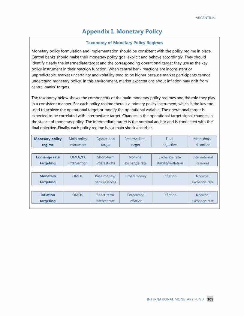
ARGENTINA


Appendix I. Monetary Policy

Taxonomy of Monetary Policy Regimes

Monetary policy formulation and implementation should be consistent with the policy regime in place.

Central banks should make their monetary policy goal explicit and behave accordingly. They should

identify clearly the intermediate target and the corresponding operational target they use as the key

policy instrument in their reaction function. When central bank reactions are inconsistent or

unpredictable, market uncertainty and volatility tend to be higher because market participants cannot

understand monetary policy. In this environment, market expectations about inflation may drift from

central banks’ targets.

The taxonomy below shows the components of the main monetary policy regimes and the role they play

in a consistent manner. For each policy regime there is a primary policy instrument, which is the key tool

used to achieve the operational target or modify the operational variable. The operational target is

expected to be correlated with intermediate target. Changes in the operational target signal changes in

the stance of monetary policy. The intermediate target is the nominal anchor and is connected with the

final objective. Finally, each policy regime has a main shock absorber.

Monetary policy

regime

Main policy

instrument

Operational

target

Intermediate

target

Final

objective

Main shock

absorber

Exchange rate

targeting

OMOs/FX

intervention

Short-term

interest rate

Nominal

exchange rate

Exchange rate

stability/inflation

International

reserves

Monetary

targeting

OMOs Base money/

bank reserves

Broad money Inflation Nominal

exchange rate

Inflation

targeting

OMOs Short-term

interest rate

Forecasted

inflation

Inflation Nominal

exchange rate

ARGENTINA


Appendix II. Turkey’s Transition to Inflation Targeting

Turkey spent almost four years building the blocks for the adoption of inflation targeting.

During this transitory period (2002 to 2005) a new central bank law was approved, which set the

institutional foundations of a more independent and forward looking monetary policy. In addition,

the Central Bank of Turkey (CBT) built institutional capacity to implement inflation targeting. By end

2005, before launching inflation targeting, inflation had declined to single digits.

The CBT implemented what it called an “implicit inflation targeting.” It announced a multiyear

inflation target consistent with targets set in the stand-by program negotiated with the IMF, and

used monetary aggregates—also negotiated with the IMF—as intermediate targets. However, the

latter would be revised if an inconsistency emerged between the final objective and the

intermediate target. The decision-making process, though, was discretionary and opaque as policy

decisions were unpredictable and not well communicated (Kara, 2006). Behind the scenes, the

central bank made important strides to improve data availability. It improved the methodology for

the calculation of the consumer price index and started to conduct surveys, in particular of inflation

expectations. As data improved, the central bank could improve the analysis of the monetary policy

transmission mechanism, and was in a better position to forecast inflation.

In the wake of the financial crisis, Turkey approved a bold reform of the central bank law. The

new law was aimed at building the blocks for a more independent monetary policy and, ultimately,

at laying the ground for adopting inflation targeting. Key provisions of the 2001 legislation were the

following: (i) clarifying the mandate of the CBT by stipulating that its primary objective is to achieve

and maintain price stability. The central bank was also assigned the mandate of maintaining financial

stability; (ii) granting political and instruments independence to the CBT by empowering it to

formulate monetary policy at its own discretion, using autonomously monetary policy instruments;

(iii) Banning central bank advances and credit to the government and the rest of the public sector,

which brought to end the monetization of fiscal deficit that fueled in the past inflation; and (iv)

Holding the central bank accountable. The governor of the CBT was required to submit twice a year

a report to the Council of Ministers and the Planned and Budget Commission of the National

Assembly on the operations of the bank and the monetary policy pursued. The CBT was also

required to inform the public and disclose the reasons for not achieving the monetary targets.

Inflation was on target by 2005, thus exceeding all expectations. With the support of a

disciplined fiscal policy, the annual inflation rate fell from 68 percent in 2001 to less than 8 percent

by end 2005—the target set for this year. At the same time, exchange rate volatility declined and so

did the country’s risk premium, while nominal and real interest rates came down and the exchange

rate pass-through weakened. These positive outcomes help strengthening the credibility of the CBT

thereby creating a favorable environment for the introduction of a full-fledged inflation targeting at

the beginning of 2006.

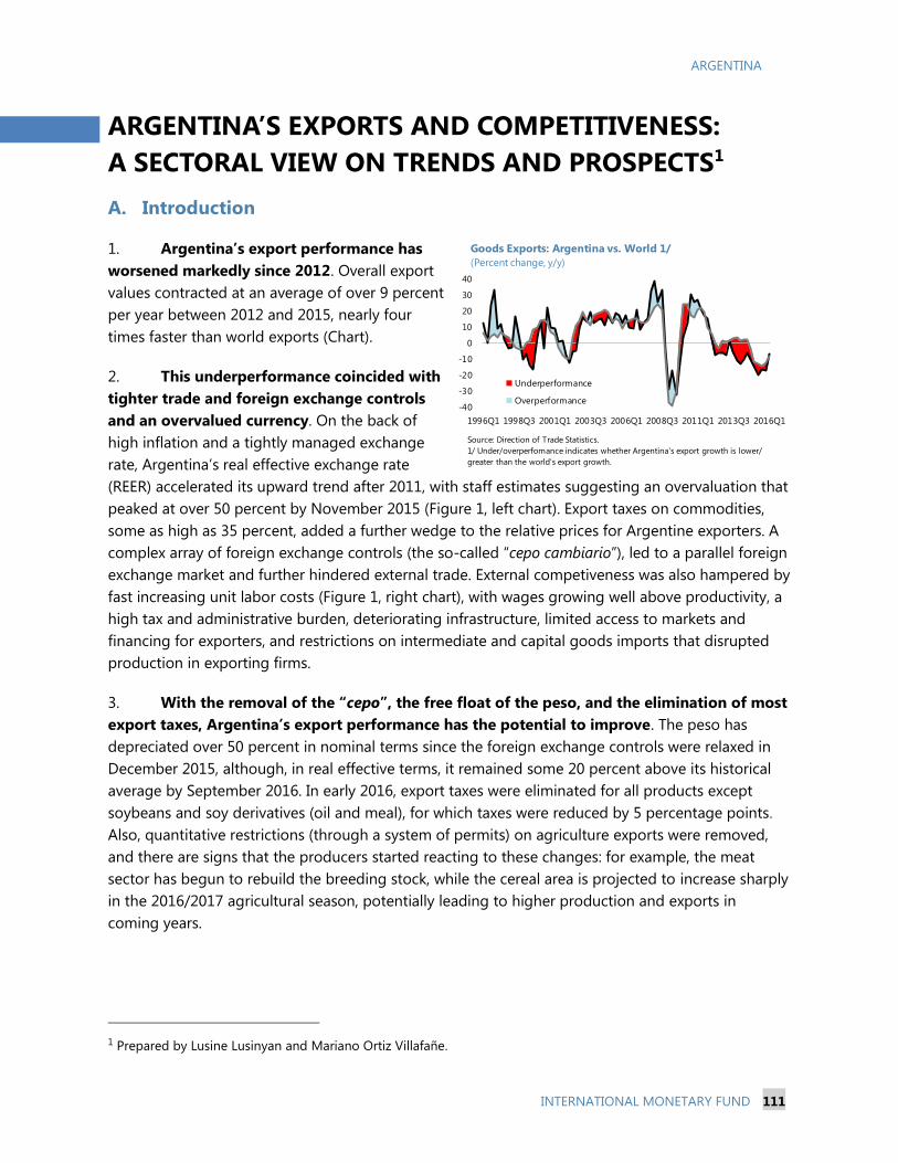
ARGENTINA


ARGENTINA’S EXPORTS AND COMPETITIVENESS:

A SECTORAL VIEW ON TRENDS AND PROSPECTS1

A. Introduction

1. Argentina’s export performance has

worsened markedly since 2012. Overall export

values contracted at an average of over 9 percent

per year between 2012 and 2015, nearly four

times faster than world exports (Chart).

2. This underperformance coincided with

tighter trade and foreign exchange controls

and an overvalued currency. On the back of

high inflation and a tightly managed exchange

rate, Argentina’s real effective exchange rate

(REER) accelerated its upward trend after 2011, with staff estimates suggesting an overvaluation that

peaked at over 50 percent by November 2015 (Figure 1, left chart). Export taxes on commodities,

some as high as 35 percent, added a further wedge to the relative prices for Argentine exporters. A

complex array of foreign exchange controls (the so-called “cepo cambiario”), led to a parallel foreign

exchange market and further hindered external trade. External competiveness was also hampered by

fast increasing unit labor costs (Figure 1, right chart), with wages growing well above productivity, a

high tax and administrative burden, deteriorating infrastructure, limited access to markets and

financing for exporters, and restrictions on intermediate and capital goods imports that disrupted

production in exporting firms.

3. With the removal of the “cepo”, the free float of the peso, and the elimination of most

export taxes, Argentina’s export performance has the potential to improve. The peso has

depreciated over 50 percent in nominal terms since the foreign exchange controls were relaxed in

December 2015, although, in real effective terms, it remained some 20 percent above its historical

average by September 2016. In early 2016, export taxes were eliminated for all products except

soybeans and soy derivatives (oil and meal), for which taxes were reduced by 5 percentage points.

Also, quantitative restrictions (through a system of permits) on agriculture exports were removed,

and there are signs that the producers started reacting to these changes: for example, the meat

sector has begun to rebuild the breeding stock, while the cereal area is projected to increase sharply

in the 2016/2017 agricultural season, potentially leading to higher production and exports in

coming years.

1 Prepared by Lusine Lusinyan and Mariano Ortiz Villafañe.

-40

-30

-20

-10

0

10

20

30

40

1996Q1 1998Q3 2001Q1 2003Q3 2006Q1 2008Q3 2011Q1 2013Q3 2016Q1

Underperformance

Overperformance

Goods Exports: Argentina vs. World 1/

(Percent change, y/y)

Source: Direction of Trade Statistics.

1/ Under/overperfomance indicates whether Argentina's export growth is lower/

greater than the world's export growth.

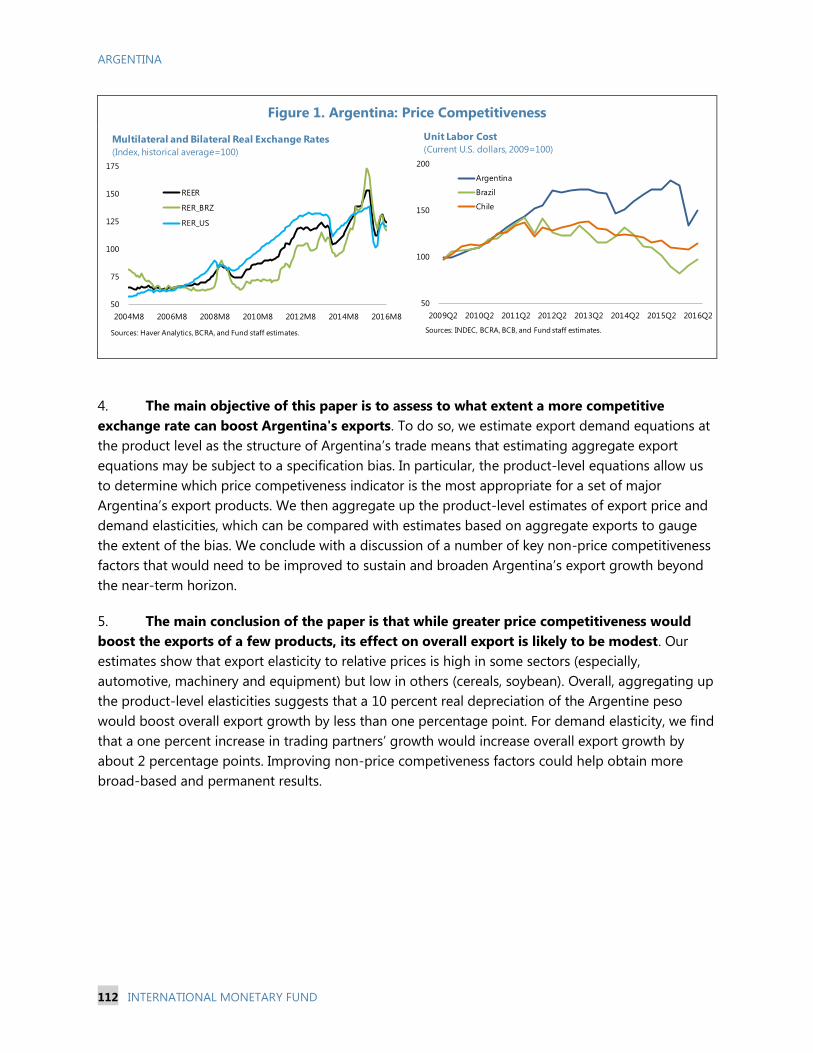
ARGENTINA


Figure 1. Argentina: Price Competitiveness

4. The main objective of this paper is to assess to what extent a more competitive

exchange rate can boost Argentina's exports. To do so, we estimate export demand equations at

the product level as the structure of Argentina’s trade means that estimating aggregate export

equations may be subject to a specification bias. In particular, the product-level equations allow us

to determine which price competiveness indicator is the most appropriate for a set of major

Argentina’s export products. We then aggregate up the product-level estimates of export price and

demand elasticities, which can be compared with estimates based on aggregate exports to gauge

the extent of the bias. We conclude with a discussion of a number of key non-price competitiveness

factors that would need to be improved to sustain and broaden Argentina’s export growth beyond

the near-term horizon.

5. The main conclusion of the paper is that while greater price competitiveness would

boost the exports of a few products, its effect on overall export is likely to be modest. Our

estimates show that export elasticity to relative prices is high in some sectors (especially,

automotive, machinery and equipment) but low in others (cereals, soybean). Overall, aggregating up

the product-level elasticities suggests that a 10 percent real depreciation of the Argentine peso

would boost overall export growth by less than one percentage point. For demand elasticity, we find

that a one percent increase in trading partners’ growth would increase overall export growth by

about 2 percentage points. Improving non-price competiveness factors could help obtain more

broad-based and permanent results.

50

75

100

125

150

175

2004M8 2006M8 2008M8 2010M8 2012M8 2014M8 2016M8

REER

RER_BRZ

RER_US

Multilateral and Bilateral Real Exchange Rates

(Index, historical average=100)

Sources: Haver Analytics, BCRA, and Fund staff estimates.

50

100

150

200

2009Q2 2010Q2 2011Q2 2012Q2 2013Q2 2014Q2 2015Q2 2016Q2

Argentina

Brazil

Chile

Unit Labor Cost

(Current U.S. dollars, 2009=100)

Sources: INDEC, BCRA, BCB, and Fund staff estimates.

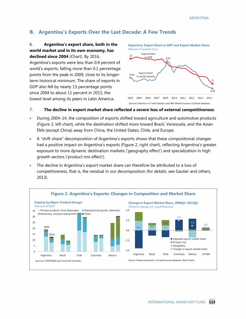
ARGENTINA


B. Argentina’s Exports Over the Last Decade: A Few Trends

6. Argentina’s export share, both in the

world market and in its own economy, has

declined since 2004 (Chart). By 2016,

Argentina’s exports were less than 0.4 percent of

world’s exports, falling more than 0.1 percentage

points from the peak in 2009, close to its longer-

term historical minimum. The share of exports in

GDP also fell by nearly 13 percentage points

since 2004 to about 11 percent in 2015, the

lowest level among its peers in Latin America.

7. The decline in export market share reflected a severe loss of external competitiveness.

During 2004–14, the composition of exports shifted toward agriculture and automotive products

(Figure 2, left chart), while the destination shifted more toward Brazil, Venezuela, and the Asian

EMs (except China) away from China, the United States, Chile, and Europe.

A “shift-share” decomposition of Argentina’s exports shows that these compositional changes

had a positive impact on Argentina’s exports (Figure 2, right chart), reflecting Argentina’s greater

exposure to more dynamic destination markets (‘geography effect’) and specialization in high

growth sectors (‘product mix effect’).

The decline in Argentina’s export market share can therefore be attributed to a loss of

competitiveness, that is, the residual in our decomposition (for details, see Gaulier and others,

2013).

Figure 2. Argentina’s Exports: Changes in Composition and Market Share

0.40

0.47

0.35

23

11

2004 2005 2006 2007 2009 2010 2011 2012 2014 2015

Argentina: Export Share in GDP and Export Market Share

(Percent, 4-quarter m.a.)

Export share

in GDP

Export share

in world exports

Sources: Direction of Trade Statistics and IMF World Economic Outlook database.

0

5

10

15

20

25

30

35

Argentina Brazil Chile Colombia Mexico

Exports by Major Product Groups

(Percent of GDP)

Primary products, food, beverages Manufactured goods, chemicals

Machinery, transport equipment Other

2004

2014

Sources: COMTRADE and Fund staff esimates.

0.10.5

1.0

2.4

1.10.7

-5.0

-2.5

0.0

2.5

5.0

Argentina Brazil Chile Colombia Mexico LATAM

Adjusted export market share

Product mix

Geography

Change in export market share

Change in Export Market Share, 2006Q1–2015Q2

(Percent change, y/y, log difference)

Source: Measuring Export Competitiveness database, World Bank.

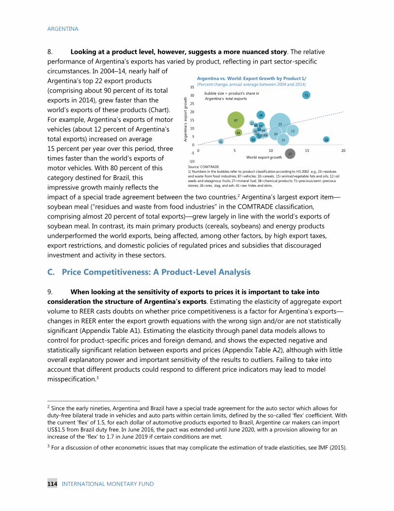
ARGENTINA


8. Looking at a product level, however, suggests a more nuanced story. The relative

performance of Argentina’s exports has varied by product, reflecting in part sector-specific

circumstances. In 2004–14, nearly half of

Argentina’s top 22 export products

(comprising about 90 percent of its total

exports in 2014), grew faster than the

world’s exports of these products (Chart).

For example, Argentina’s exports of motor

vehicles (about 12 percent of Argentina’s

total exports) increased on average

15 percent per year over this period, three

times faster than the world’s exports of

motor vehicles. With 80 percent of this

category destined for Brazil, this

impressive growth mainly reflects the

impact of a special trade agreement between the two countries.2 Argentina’s largest export item—

soybean meal (“residues and waste from food industries” in the COMTRADE classification,

comprising almost 20 percent of total exports)—grew largely in line with the world’s exports of

soybean meal. In contrast, its main primary products (cereals, soybeans) and energy products

underperformed the world exports, being affected, among other factors, by high export taxes,

export restrictions, and domestic policies of regulated prices and subsidies that discouraged

investment and activity in these sectors.

C. Price Competitiveness: A Product-Level Analysis

9. When looking at the sensitivity of exports to prices it is important to take into

consideration the structure of Argentina’s exports. Estimating the elasticity of aggregate export

volume to REER casts doubts on whether price competitiveness is a factor for Argentina’s exports—

changes in REER enter the export growth equations with the wrong sign and/or are not statistically

significant (Appendix Table A1). Estimating the elasticity through panel data models allows to

control for product-specific prices and foreign demand, and shows the expected negative and

statistically significant relation between exports and prices (Appendix Table A2), although with little

overall explanatory power and important sensitivity of the results to outliers. Failing to take into

account that different products could respond to different price indicators may lead to model

misspecification.3

2 Since the early nineties, Argentina and Brazil have a special trade agreement for the auto sector which allows for

duty-free bilateral trade in vehicles and auto parts within certain limits, defined by the so-called ‘flex’ coefficient. With

the current ‘flex’ of 1.5, for each dollar of automotive products exported to Brazil, Argentine car makers can import

US$1.5 from Brazil duty free. In June 2016, the pact was extended until June 2020, with a provision allowing for an

increase of the ‘flex’ to 1.7 in June 2019 if certain conditions are met.

3 For a discussion of other econometric issues that may complicate the estimation of trade elasticities, see IMF (2015).

2387

10

15

12

27

38

71

99

0284 03

04

39 26

0873

20

41

22

30

33

-10

-5

0

5

10

15

20

25

30

35

0 5 10 15 20

World export growth

Arg

entina's

exp

ort

gro

wth

bubble size = product's share in

Argentina's total exports

Argentina vs. World: Export Growth by Product 1/

(Percent change, annual average between 2004 and 2014)

Source: COMTRADE.

1/ Numbers in the bubbles refer to product classification according to HS 2002: e.g., 23=residues

and waste from food industries; 87=vehicles; 10=cereals; 15=animal/vegetable fats and oils; 12=oil

seeds and oleaginous fruits; 27=mineral fuel; 38=chemical products; 71=precious/semi-precious

stones; 26=ores, slag, and ash; 41=raw hides and skins.

ARGENTINA


10. In this paper, we estimate export growth equations at product level, using different

indicators of relative prices for each product.4 For example, soybean meal represents about

20 percent of Argentina’s overall exports but very little of this product is exported to the top 10

trade partners of Argentina. This suggests that REER, which uses total export shares as the weights,

may not be the best price competitiveness indicators for this product. Instead, the demand for this

product is likely to depend more on its export price (in absolute terms, or relative to the prices in the

export destination countries) and the cost structure relative to main competitors. Since both

Argentina and Brazil have relatively large market shares in total world exports of soybean meal (36

and 22 percent, respectively), the demand for Argentina’s export of this product could be

particularly affected by its bilateral real exchange rate with Brazil (facing the same level of

international prices, the country with a lower relative cost of production should be able to produce

and export more). For transport equipment, Argentina’s second largest export item, the bilateral real

exchange rate with Brazil would be the most appropriate price indicator given that 80 percent of the

exports of this product goes to Brazil, and large car manufacturers operating in both countries can

potentially react to changes in their relative cost structure.5

11. In particular, for each product p, we estimate the following equation:

∆𝑋𝑝,𝑡 = 𝛽𝑝,0 + 𝛽𝑝,1∆�̅�𝑝,𝑡 + 𝛽𝑝,2∆𝑃𝑝,𝑡 + 𝜑𝑝,𝑡 + 𝜏𝑝,𝑡 + 𝜎𝑡 + 𝜖𝑝,𝑡 (1)

where 𝑋𝑝,𝑡 is Argentina’s export volume; �̅�𝑝,𝑡 is the demand for that product from Argentina trading

partners (using export share as weights); 𝑃𝑝,𝑡 are indicators of price competitiveness as described

below; 𝜑𝑝,𝑡 is product-specific factors, such as harvest-related factors; 𝜎𝑡 is country-wide factors

affecting exports, such as exchange rate uncertainty; 𝜏𝑝,𝑡 are time dummies (where significant); and

𝜖𝑝,𝑡 is the error term.6 For the sources and description of the data, see Appendix 1. The variables

denoted by ∆ are growth rates calculated as quarterly year-on-year log differences. Eq. (1) is

estimated with OLS with robust standard errors, or Prais-Winston GLS estimator to correct for the

first-order error autocorrelation when such is detected in residual diagnostic tests. The sample

period is 2004Q1–2016Q2, reflecting the availability of product-level export data. The choice of a

proxy for price competitiveness or relative prices is not straightforward, and most studies simply use

4 The differences among Argentina’s main export products were emphasized in Catão and Falcetti (1999). In

particular, they argued that, given the specific features of manufacturing trade within the South American common

market (MERCOSUR), Argentina’s exports comprise two different groups of products in terms of their economic

determinants: while the price of exports of primary and lightly manufactured goods is largely determined at the

world market, Argentina’s industrial exports (to MERCOSUR) are mostly influenced by such factors as intra-bloc trade

policies, income growth in the region, and geographical proximity. Consequently, they use two different

specifications for the export functions—an export supply function for total exports excluding manufacturing exports

to Brazil, and a two-equation, supply-and-demand system for manufacturing exports to Brazil.

5 If both currencies appreciate and the bilateral real exchange rate remains unchanged, Brazilian importers would still

find difficult to switch to non-Argentine products owing to the very high (up to 35 percent) tariffs in the auto sector.

6 Note also that this specification differs from more standard export demand equations which use the level of real

exports as a dependent variable. The aggregate product-level data from INDEC, which we would like to explore in

this chapter, are available as indices (see Appendix 1).

ARGENTINA


the indicator with the best fit.7 Ideally, the relative price would capture not only the relation between

export prices of the home country and domestic prices of the trading partners, but also the export

price of the home country relative to export price of potential competitors.8 We use the following

price indicators:

Real effective exchange rate (REER), CPI (or GDP deflator) based, defined as 𝑒𝑡𝑃𝐴𝑟𝑔,𝑡

�̅�𝑝,𝑡$ , where 𝑒𝑡 is

the nominal exchange rate (U.S. dollars per peso), 𝑃𝐴𝑟𝑔,𝑡 is Argentina’s prices (CPI or GDP

deflator), and �̅�𝑝,𝑡$ is product-specific export share-weighted foreign U.S. dollar prices (CPI or

GDP deflator);

Bilateral real exchange rate with respect to the Brazilian real, similar to REER but the

denominator represents only the U.S. dollar prices in Brazil;

Export prices, product-specific unit value prices of Argentina’s exports in U.S. dollar, 𝑃𝑝,𝑡𝑋 ;

Relative export prices defined as 𝑃𝑝,𝑡

𝑋

�̅�𝑝,𝑡$ ; and

Commodity exporter exchange rates, a proxy of the relative prices faced by Argentina’s exporters.

calculated as 𝑃𝑝,𝑡

∗ (1−𝜏𝑝,𝑡)

𝑒𝑡𝑃𝐴𝑟𝑔,𝑡, namely the ratio of the international price of a given product, 𝑃𝑝,𝑡

∗ ,

adjusted for Argentina’s (time-varying) export tax rate, 𝜏𝑝,𝑡, to Argentina’s domestic prices in U.S.

dollars. An increase in this ratio as a result of higher international price, lower tax rate, lower

domestic inflation, or nominal depreciation of the peso would imply more favorable relative

prices for the Argentine commodity exporters.

12. The results confirm that different products tend to react to different indicators of

price competitiveness (Appendix Table A3). The final specification for each product has been

selected based on its fit (measured through R2 and RMSE), which in most cases also matches the

characteristics of trade. The fit of the estimated equations for six largest export products (which

comprise about two-thirds of Argentina’s total exports) is shown in Appendix Figure A2.9 Among the

main results we find that:

7 See, for example, Senhadji and Montenegro (1998) and Catão and Falcetti (1999).

8 Furthermore, as a measure of domestic price of importers, it would be more preferable to use producer price

indices (PPIs), which however are not readily available for all the countries in our sample, and we use CPI or GDP

deflator indices instead. However, IMF (2015) finds that using CPI instead of PPI does not significantly impact the

estimated trade elasticities.

9 For products for which Argentina enjoys a large export market share, such as soybean oil, a system of export supply

and demand equations is also estimated (not reported here) which yields largely similar results.

ARGENTINA


For exports of automotive sector, chemicals, and machinery/equipment, the relative price that

matters is the RER with the Brazilian real with an estimated elasticity of about -0.3.

Exports of soybean meal depend on international export prices and the bilateral real exchange

rate with the Brazilian real, in line with our expectations. For soybean oil (fats and oils in

Appendix Table A3), export depend on international prices only, reflecting the fact that

Argentina has the largest market share in the world (40 percent of total world exports) and is

therefore a price setter. Exports of cereals (mainly corn) depend on the commodity exporter

exchange rate (though less robustly), consistent with the hypothesis that export taxes

particularly affected the export of this product which (unlike soybean meal) is also consumed

domestically.

Export sensitivity to trading partner growth appears to be particularly high for automotive,

machinery/equipment, and soybean. For soybean meal, partner demand does not appear to be

very robust, which in part can reflect the fact that some countries (like the Netherlands) are

among the main importers of this product but part of the imports is being re-exported to the

markets of final consumptions.

Rainfall is a key determinant of export supply for all agriculture products, while a negative

downward trend is detected for export growth in basic metals and meat. Export regressions, not

surprisingly, perform relatively poorly for the energy sector, reflecting distortions introduced by

the domestic energy policies.

Exchange rate uncertainty, proxied by the unconditional three-quarter moving standard

deviation of REER (but also nominal or parallel exchange rates) does not appear to be robust in

export equations (unlike Catão and Falcetti, 1999, who however cover a much earlier period).

13. The export elasticity to REER derived from aggregating up these product-specific

elasticities is relatively low. To gauge the aggregate export elasticity to REER, we perform a simple

simulation exercise. First, we calculate export growth rates for each product using the elasticity

estimates from the regressions and the forecast of the determinants (relative prices and trading

partner growth) from the latest (October 2016) World Economic Outlook projections. Then, we derive

the projected growth rate for the overall exports, as the weighted sum of product-level projections,

using export shares as weights.10 Third, we re-calculate export growth rates for those products for

which the price indicator depends on the exchange rate using a modified path of the nominal

exchange rate, which implies a 10 percent depreciation in real effective terms in 2017 relative to the

baseline, and aggregate again to get a projection of overall export growth. The difference between

the two projected overall export growth rates yields an approximate elasticity of total exports

growth to the change in REER. We use a similar approach to estimate the demand elasticity of the

aggregate exports. Our findings suggest that that 10 percent real depreciation of the Argentine

10 The assumption of unchanged export shares following exchange rate devaluation appears appropriate for deriving

aggregate export growth projections over a short-term horizon given that sectoral restructuring will likely to take

time, the changes to export shares observed in the first half of 2016 (mainly favoring cereals and soybean/oil), and

the evidence from Argentine exports’ reaction following the 2002 devaluation.

ARGENTINA


peso would boost total exports growth by less than one percentage point, and a one percent

increase in trading partner growth is associated with about 2 percentage points higher total export

growth. While price elasticity of exports appears on the lower side of estimates found in the

literature, our estimate of demand elasticity is close to the average for a number of other emerging

market economies (see, for example, IMF, 2015).

D. Non-Price Competitiveness: A Few Considerations

14. Interventionist policies over the past years contributed to the weak export

performance, suggesting that their removal could help improve external competitiveness.

Quantifying the potential gains to exports from the removal of the restrictions associated with the

cepo cambiario is not straightforward, mainly as the cepo came on top of other restrictions that had

already been in place for much of the last decade (for example, exports of meat, cereals and other

agricultural products, have been subject to quotas since 2006). Still, our product-level regressions

over-estimate actual export growth after 2012 for a series of products with relatively higher import

content, such as chemicals, machinery and equipment, and plastic products—suggesting that import

restrictions affecting industrial inputs disrupted production and exports of these manufactured

goods (Appendix Figure A3). Focusing on these products, our simulations suggest that the annual

average growth in total exports could have been ½ percentage points higher in 2012–15 without

the restrictions imposed by the cepo.11

15. While potential gains from price competitiveness appear to be modest for Argentina’s

exports, non-price factors could play a significant role in enhancing its external

competitiveness. External competiveness and the evolution of global market shares can be

explained only partially by looking at changes in price competiveness (Benkovskis and Worz, 2013).

A series of non-price factors could have a substantial positive impact on export performance,

including improving the quality of infrastructure, reducing tax pressure and administrative burden,

easing access to financing, and pursuing trade policies that facilitate market access.

Tax regime. At 34 percent of GDP (in 2015), the tax burden in Argentina is one of the highest in

the region and among emerging market economies. In the food industry, the key export sector,

taxes and social security contributions comprised an estimated 58 percent of the value added

(COPAL, 2015). Immediately after taking office, the current government started to address this

issue by eliminating or reducing export duties,12 thus improving the effective exchange rate the

11 In this simulation, we assume that the difference in the actual and fitted values of growth in exports of chemicals,

machinery and equipment, and plastic products in 2012–15 is fully attributed to the effects of restrictions, and that

the exports of these products (which together comprise about 13 percent to total exports) grew as projected by the

model after 2012. The choice of these sectors has also been confirmed through a t-test on the equality of means of

regression residuals before and after 2012Q1, showing that the average residuals after 2012Q1 (included) were

significantly different and smaller than the average residuals before 2012.

12 In mid-December 2015, the new administration eliminated export duties on most products except for soybeans

and soy derivatives, which were reduced by 5 percentage points. The system of export permits for agricultural

exports was also removed.

ARGENTINA


exporters perceive. However, there is still room for improvement, as corporate income taxation

is not designed to stimulate investment, while the large tax wedge makes labor expensive.

Infrastructure and logistics. Although infrastructure access in Argentina is above the regional

average, infrastructure quality has declined

steadily over the past years. The World

Economic Forum (WEF) ranking of

infrastructure quality shows that between

2006 and 2015 Argentina lost 62 positions,

falling from 61 to 123. Over the past 15 years,

public investment grew much less than other

types of spending, such as subsidies to

energy and transportation, while private

financing of infrastructure was very limited

(World Bank, 2015). Access to appropriate

infrastructure in terms of roads, railways,

ports and energy is especially important for exporting firms outside the central region and

metropolitan areas, which tend to be the most vulnerable to REER appreciation. The logistic cost

of exporting a 40-foot container by land is US$1,842 in Argentina compared to US$1,000 in

Brazil, with data as of 2014 (World Bank, 2015). According to the World Bank Logistics

Performance Index (LPI), Argentina’s gap with the best performing OECD country is about

1 point and 0.3 points with the average of its peers,13 and improving the LPI score by 1 could

increase labor productivity by close to 35 percent on average (OECD, CAF, and ECLAC, 2013).

Administrative procedures. Excessive

bureaucracy, lack of coordination between

government agencies, and inefficient

customs systems undermine export

competitiveness by increasing transaction

costs. Argentine exporters face comparatively

high costs to export, according to the World

Development Indicators (WDI) index that

measures the fees associated with

completing the export procedures (Chart).14

Trade policy. A dynamic and ambitious

trade policy can substantially improve export performance by expanding market access for

domestic exporting firms and facilitating their integration into global value chains. As part of the

MERCOSUR trade bloc, in recent years Argentina has lagged behind other regional peers, such

as the members of the Pacific Alliance (Chile, Mexico, Colombia and Peru), which have been

13 The LPI has a scale of 1 to 5, where 5 represents the best logistics performance.

14 The fees covered include costs for documents, administrative fees for customs clearance and technical control,

customs broker fees, terminal handling charges and inland transport, but does not include tariffs or trade taxes.

ARG

BRZ

CHL

URY

AUS

CHN

IND

NZL

-0.2

0.0

0.2

0.4

0.6

500 1,000 1,500 2,000 2,500

Change in Export Market Share and Administrative Costs

Administrative cost to export (U.S. dollar per container)

Chang

ein

mark

et

share

, 2005

–14 (

log

dif

f)

Sources: Direction of Trade Statistics and World Development Indicators (2014).

ARG

BRZ

CHL

URY

AUS

CHNIND

NZL

-0.2

0.0

0.2

0.4

0.6

2 3 4 5 6

Change in Export Market Share and Transport Infrastructure

Quality of transport infrastructure (7=best)

Chang

ein

mark

et

share

, 2005–14 (

log

diff)

Sources: Direction of Trade Statistics and Global Competitiveness Report (2014).

ARGENTINA


more aggressive in securing new export markets.15 More recently, seeking closer relationships

with the Pacific Alliance and advancing the trade negotiations between MERCOSUR and the EU

might mark a shift in trade policy.

Access to financing. Recent studies confirm that access to bank credit is important for the

decision to enter export markets. And access to foreign financing helps firms to reach more

developed and more distant markets, increasing also the number of destinations and of

products exported (Castagnino, D’Amato, and Sangiácomo, 2013). The underdevelopment of the

Argentina’s financial system, which is small and mostly transactional, combined with limited

access to international capital markets, has affected export competitiveness of local firms in

recent years. The recent resolution of the holdouts conflict, following the settlement with the

Paris Club in 2014 marked a crucial step in the financial normalization process that will likely

pave the way to increase external trade financing to Argentine exporters.

15 Argentina currently has trade agreements with 43 countries, while Chile has agreements with 91 countries.

ARGENTINA


References

Benkovskis, K., and J. Worz (2013), Non-Price Competitiveness in Exports from Emerging Countries,

European Central Bank WP Series, No. 1612.

Castagnino, T., D’Amato, L., and M. Sangiácomo (2013), How Do Firms in Argentina Get Financing to

Export? European Central Bank WP Series, No. 1601.

Catão, L., and E. Falcetti (1999), Determinants of Argentina’s External Trade, IMF Working Paper

WP/99/121, International Monetary Fund.

COPAL (2015), Análisis y Propuestas de Políticas Públicas de COPAL para la Industria de Alimentos y

Bebidas, Coordinadora de las Industrias de Productos Alimenticios.

Gaulier, G., Santoni, G., Taglioni, D., and S. Zignago (2013), In the Wake of the Global Crisis Evidence

from a New Quarterly Database of Export Competitiveness, World Bank Policy Research

Working Paper, WPS 6733.

International Monetary Fund (2015), World Economic Outlook, Chapter 3 “Exchange Rates and Trade

Flows: Disconnected?” October, International Monetary Fund.

OECD, CAF, and ECLAC (2013), Latin American Economic Outlook 2014: Logistics and Competitiveness

for Development, OECD Publishing, Paris.

Senhadji, A., and C. Montenegro (1998), Time Series Analysis of Export Demand Equations: A Cross-

Country Analysis, IMF Working Paper 98/149, International Monetary Fund.

World Bank (2015), Public Policy Notes for Development: Argentina.

ARGENTINA


Appendix I. Data Sources and Description

Argentina’s exports: Argentina’s export volume data are based on the monthly export volume

indices available from INDEC for 39 groups of products.

Argentina’s prices: The CPI is constructed using the official INDEC GBA index until 2006M12,

appended by the private estimates of inflation until 2012M8, and the City of Buenos Aires CPI

thereafter.

Product-specific trading partner weights: The weights are derived from the COMTRADE exports

data for 2014. To obtain the weights consistent with the exports according to INDEC product

classification, the COMTRADE HS2002 level-2 product classification, which includes 97 product

categories, is mapped to the INDEC classification. Export data for Argentina vis-à-vis 182 partner

countries/areas are presented as 32 individual partner countries, which comprised about 83 percent

of Argentina’s total exports in 2014, and a group of other countries/areas.

Trading partner demand: External demand is proxied by the real GDP of the trading partners, using

the quarterly data (in constant 2010 prices and exchange rate) available from the WEO dataset. For

each product, total foreign demand is calculated as the product-specific export share-weighted

average of real GDP of the 32 partner countries.

Foreign U.S. dollar prices: Foreign price indices are the quarterly CPI data (2010 base year)

available from the WEO database. For each product, foreign U.S. dollar prices are calculated as the

product-specific export share-weighted average of the CPI of the 32 partner countries.

Rainfall: The indicator is constructed using data on monthly rainfall in a group of five weather

stations representing the main grain production area of the country. The indicator for each period

reflects the relevant rainfall for the corresponding harvest, taking into account the crop annual cycle

for oilseeds and cereals.

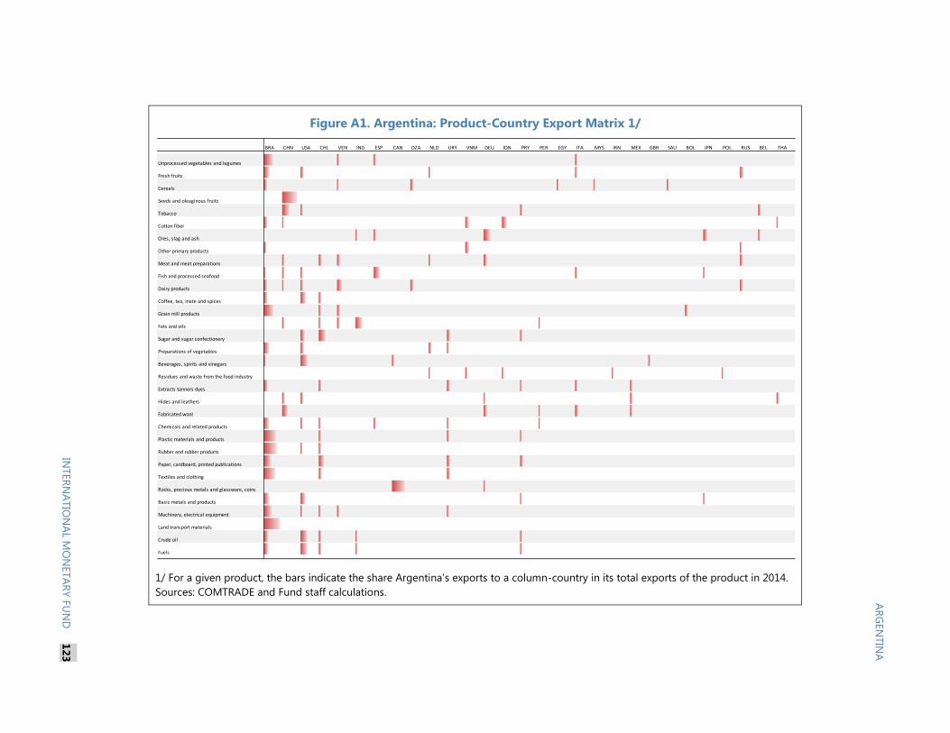
Figure A1. Argentina: Product-Country Export Matrix 1/

1/ For a given product, the bars indicate the share Argentina’s exports to a column-country in its total exports of the product in 2014.

Sources: COMTRADE and Fund staff calculations.

BRA CHN USA CHL VEN IND ESP CAN DZA NLD URY VNM DEU IDN PRY PER EGY ITA MYS IRN MEX GBR SAU BOL JPN POL RUS BEL THA

Unprocessed vegetables and legumes

Fresh fruits

Cereals

Seeds and oleaginous fruits

Tobacco

Cotton fiber

Ores, slag and ash

Other primary products

Meat and meat preparations

Fish and processed seafood

Dairy products

Coffee, tea, mate and spices

Grain mill products

Fats and oils

Sugar and sugar confectionery

Preparations of vegetables

Beverages, spirits and vinegars

Residues and waste from the food industry

Extracts tanners dyes

Hides and leathers

Fabricated wool

Chemicals and related products

Plastic materials and products

Rubber and rubber products

Paper, cardboard, printed publications

Textiles and clothing

Rocks, precious metals and glassware, coins

Basic metals and products

Machinery, electrical equipment

Land transport materials

Crude oil

Fuels

AR

GEN

TIN

A

INTER

NA

TIO

NA

L MO

NETA

RY F

UN

D 1

23

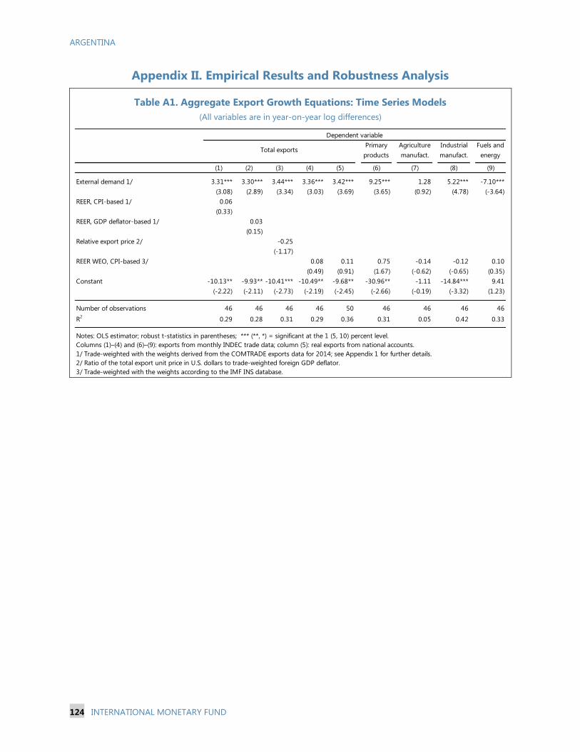
ARGENTINA


Appendix II. Empirical Results and Robustness Analysis

Table A1. Aggregate Export Growth Equations: Time Series Models

(All variables are in year-on-year log differences)

Primary

products

Agriculture

manufact.

Industrial

manufact.

Fuels and

energy

(1) (2) (3) (4) (5) (6) (7) (8) (9)

External demand 1/ 3.31*** 3.30*** 3.44*** 3.36*** 3.42*** 9.25*** 1.28 5.22*** -7.10***

(3.08) (2.89) (3.34) (3.03) (3.69) (3.65) (0.92) (4.78) (-3.64)

REER, CPI-based 1/ 0.06

(0.33)

REER, GDP deflator-based 1/ 0.03

(0.15)

Relative export price 2/ -0.25

(-1.17)

REER WEO, CPI-based 3/ 0.08 0.11 0.75 -0.14 -0.12 0.10

(0.49) (0.91) (1.67) (-0.62) (-0.65) (0.35)

Constant -10.13** -9.93** -10.41*** -10.49** -9.68** -30.96** -1.11 -14.84*** 9.41

(-2.22) (-2.11) (-2.73) (-2.19) (-2.45) (-2.66) (-0.19) (-3.32) (1.23)

Number of observations 46 46 46 46 50 46 46 46 46

R2

0.29 0.28 0.31 0.29 0.36 0.31 0.05 0.42 0.33

Notes: OLS estimator; robust t-statistics in parentheses; *** (**, *) = significant at the 1 (5, 10) percent level.

Columns (1)–(4) and (6)–(9): exports from monthly INDEC trade data; column (5): real exports from national accounts.

1/ Trade-weighted with the weights derived from the COMTRADE exports data for 2014; see Appendix 1 for further details.

2/ Ratio of the total export unit price in U.S. dollars to trade-weighted foreign GDP deflator.

3/ Trade-weighted with the weights according to the IMF INS database.

Dependent variable

Total exports

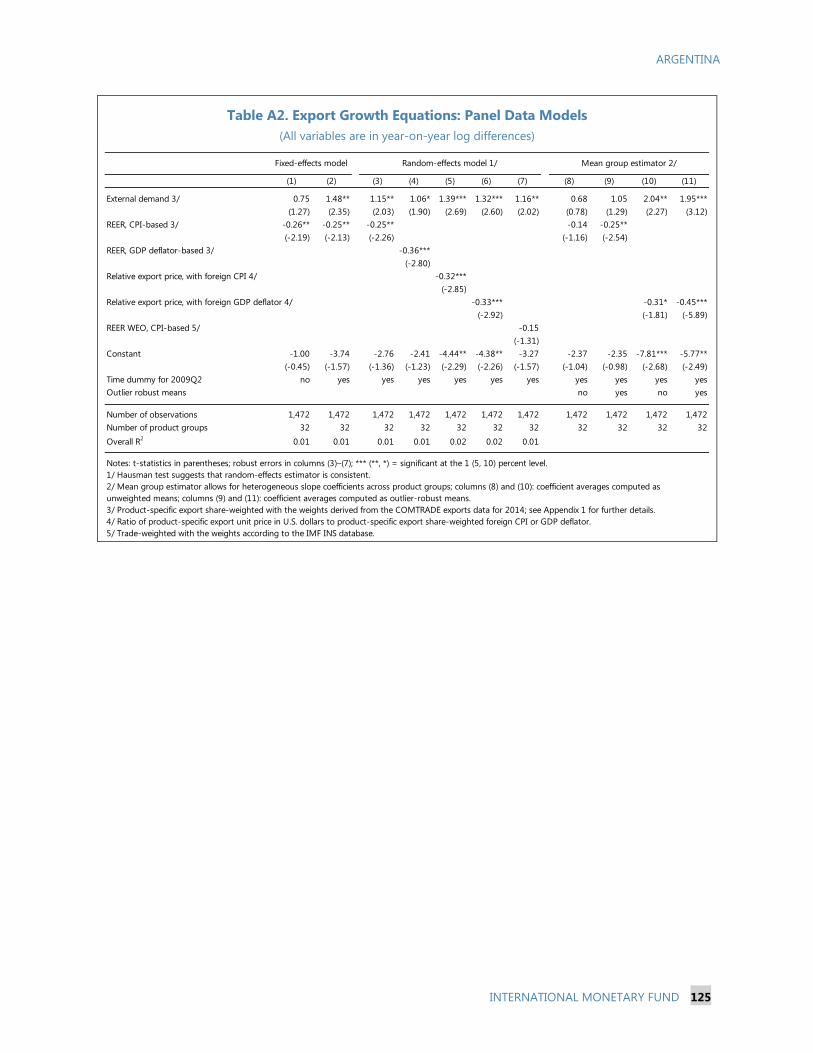
ARGENTINA


Table A2. Export Growth Equations: Panel Data Models

(All variables are in year-on-year log differences)

(1) (2) (3) (4) (5) (6) (7) (8) (9) (10) (11)

External demand 3/ 0.75 1.48** 1.15** 1.06* 1.39*** 1.32*** 1.16** 0.68 1.05 2.04** 1.95***

(1.27) (2.35) (2.03) (1.90) (2.69) (2.60) (2.02) (0.78) (1.29) (2.27) (3.12)

REER, CPI-based 3/ -0.26** -0.25** -0.25** -0.14 -0.25**

(-2.19) (-2.13) (-2.26) (-1.16) (-2.54)

REER, GDP deflator-based 3/ -0.36***

(-2.80)

Relative export price, with foreign CPI 4/ -0.32***

(-2.85)

Relative export price, with foreign GDP deflator 4/ -0.33*** -0.31* -0.45***

(-2.92) (-1.81) (-5.89)

REER WEO, CPI-based 5/ -0.15

(-1.31)

Constant -1.00 -3.74 -2.76 -2.41 -4.44** -4.38** -3.27 -2.37 -2.35 -7.81*** -5.77**

(-0.45) (-1.57) (-1.36) (-1.23) (-2.29) (-2.26) (-1.57) (-1.04) (-0.98) (-2.68) (-2.49)

Time dummy for 2009Q2 no yes yes yes yes yes yes yes yes yes yes

Outlier robust means no yes no yes

Number of observations 1,472 1,472 1,472 1,472 1,472 1,472 1,472 1,472 1,472 1,472 1,472

Number of product groups 32 32 32 32 32 32 32 32 32 32 32

Overall R2

0.01 0.01 0.01 0.01 0.02 0.02 0.01

Notes: t-statistics in parentheses; robust errors in columns (3)–(7); *** (**, *) = significant at the 1 (5, 10) percent level.

1/ Hausman test suggests that random-effects estimator is consistent.

2/ Mean group estimator allows for heterogeneous slope coefficients across product groups; columns (8) and (10): coefficient averages computed as

unweighted means; columns (9) and (11): coefficient averages computed as outlier-robust means.

3/ Product-specific export share-weighted with the weights derived from the COMTRADE exports data for 2014; see Appendix 1 for further details.

4/ Ratio of product-specific export unit price in U.S. dollars to product-specific export share-weighted foreign CPI or GDP deflator.

5/ Trade-weighted with the weights according to the IMF INS database.

Mean group estimator 2/Fixed-effects model Random-effects model 1/

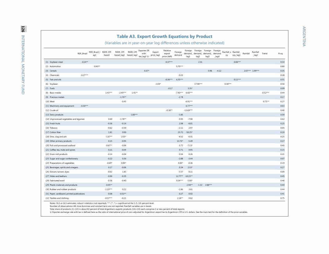
AR

GEN

TIN

A

Table A3. Export Growth Equations by Product

(Variables are in year-on-year log differences unless otherwise indicated)

RER_BrazilRER_Brazil_l

ag1

REER, CPI

based

REER, CPI

based_lag1

REER, CPI

based_lag2

Exporter ER

with

tax_lag2 1/

Export

price_lag1

Relative

export

price (defl)

Foreign

demand

Foreign

demand_

lag1

Foreign

demand_

lag2

Foreign

demand_

lag3

Foreign

demand

_lag4

Rainfall_s

oy

Rainfall_

soy_lag1Rainfall

Rainfall

_lag2Trend R-sq.

(1) Soybean meal -0.24** -0.37*** 2.31 0.06*** 0.54

(2) Automotive -0.43** 5.70*** 0.80

(3) Cereals 0.37* 5.98 -4.12 2.07*** 1.99*** 0.35

(4) Chemicals -0.27*** -0.22 0.28

(5) Fats and oils -0.36*** 6.35*** 0.11*** 0.51

(6) Soybean -1.03* 17.90*** 0.30*** 0.56

(7) Fuels -0.17 3.35* 0.09

(8) Basic metals 1.43*** -2.49*** 1.41** -7.40*** 6.60*** -0.52*** 0.44

(9) Precious metals -1.70** -2.78 0.17

(10) Meat -0.45 -6.91*** -0.71** 0.27

(11) Machinery and equipment -0.30*** 6.77*** 0.63

(12) Crude oil -0.38** -13.69*** 0.40

(13) Dairy products 1.00*** -1.85 0.59

(14) Unprocessed vegetables and legumes 0.69 -1.78** 0.95 -7.90 0.62

(15) Fresh fruits -0.36 -0.14 2.98 -0.01 0.25

(16) Tobacco -0.62 -0.59 -2.11 2.97 0.05

(17) Cotton fiber 1.81 0.00 25.72 -50.25* 0.10

(18) Ores, slag and ash -1.67** 2.03* -4.52 -0.31 0.25

(19) Other primary products 0.15 -0.95 13.73* -5.49 0.17

(20) Fish and processed seafood -0.67** -0.06 5.72 -7.13* 0.45

(21) Coffee, tea, mate and spices 0.21 -0.04 0.71 0.95 0.15

(22) Grain mill products -0.14 -0.04 0.34 0.26 0.31

(23) Sugar and sugar confectionery -0.22 0.36 -2.88 -3.44 0.07

(24) Preparations of vegetables -0.69* 0.84* 4.84* -0.36 0.19

(25) Beverages, spirits and vinegars 0.17 -0.06 0.34 2.53* 0.27

(26) Extracts tanners dyes -0.02 1.85 -5.57 8.11 0.09

(27) Hides and leathers -0.06 -0.35 12.77** -10.15** 0.45

(28) Fabricated wool -0.36 -0.40 9.34*** -5.00* 0.48

(29) Plastic materials and products -0.45** -2.94** -1.32 2.88*** 0.44

(30) Rubber and rubber products -1.19*** 0.22 -1.86 3.61 0.44

(31) Paper, cardboard, printed publications -0.08 -0.53** 0.27 0.92 0.41

(32) Textiles and clothing -0.57*** -0.21 2.18** 0.62 0.75

Notes: OLS or GLS estimates; robust t-statistics (not reported); *** (**, *) = significant at the 1 (5, 10) percent level.

Number of observations=46; time dummies and constant term are not reported. Rainfall variables are in levels.

Total share of products (1)–(13) is about 82 percent of total Argentina's exports; products (14)–(32) each comprise 2 or less percent of total exports.

1/ Exporter exchange rate with tax is defined here as the ratio of international price of corn adjusted for Argentina's export tax to Argentina's CPI in U.S. dollars. See the main text for the definition of the price variables.

12

6

INTER

NA

TIO

NA

L MO

NETA

RY F

UN

D

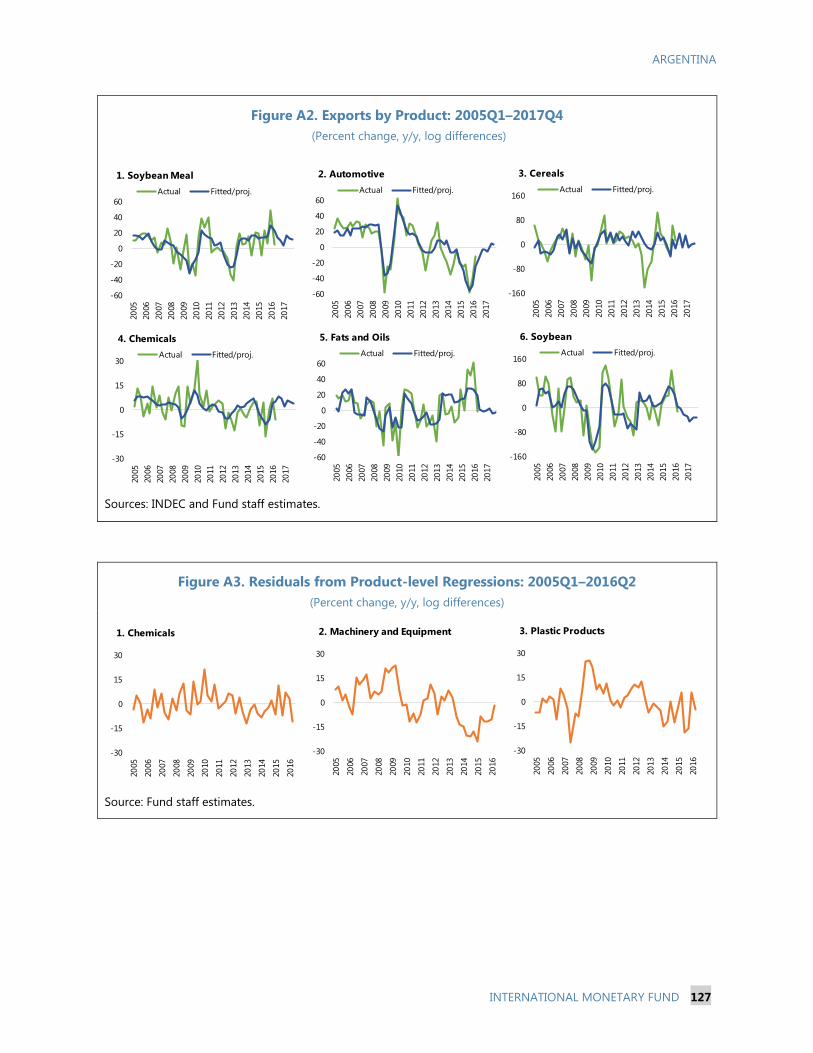
ARGENTINA


AR

GEN

TIN

A

Figure A2. Exports by Product: 2005Q1–2017Q4

(Percent change, y/y, log differences)

Sources: INDEC and Fund staff estimates.

Figure A3. Residuals from Product-level Regressions: 2005Q1–2016Q2

(Percent change, y/y, log differences)

Source: Fund staff estimates.

-60

-40

-20

0

20

40

60

20

05

20

06

20

07

20

08

20

09

20

10

20

11

20

12

20

13

20

14

20

15

20

16

20

17

1. Soybean Meal

Actual Fitted/proj.

-60

-40

-20

0

20

40

60

20

05

20

06

20

07

20

08

20

09

20

10

20

11

20

12

20

13

20

14

20

15

20

16

20

17

2. Automotive

Actual Fitted/proj.

-160

-80

0

80

160

20

05

20

06

20

07

20

08

20

09

20

10

20

11

20

12

20

13

20

14

20

15

20

16

20

17

3. Cereals

Actual Fitted/proj.

-30

-15

0

15

30

20

05

20

06

20

07

20

08

20

09

20

10

20

11

20

12

20

13

20

14

20

15

20

16

20

17

4. Chemicals

Actual Fitted/proj.

-60

-40

-20

0

20

40

60

20

05

20

06

20

07

20

08

20

09

20

10

20

11

20

12

20

13

20

14

20

15

20

16

20

17

5. Fats and Oils

Actual Fitted/proj.

-160

-80

0

80

160

20

05

20

06

20

07

20

08

20

09

20

10

20

11

20

12

20

13

20

14

20

15

20

16

20

17

6. Soybean

Actual Fitted/proj.

-30

-15

0

15

30

20

05

20

06

20

07

20

08

20

09

20

10

20

11

20

12

20

13

20

14

20

15

20

16

1. Chemicals

-30

-15

0

15

30

20

05

20

06

20

07

20

08

20

09

20

10

20

11

20

12

20

13

20

14

20

15

20

16

2. Machinery and Equipment

-30

-15

0

15

30

20

05

20

06

20

07

20

08

20

09

20

10

20

11

20

12

20

13

20

14

20

15

20

16

3. Plastic Products

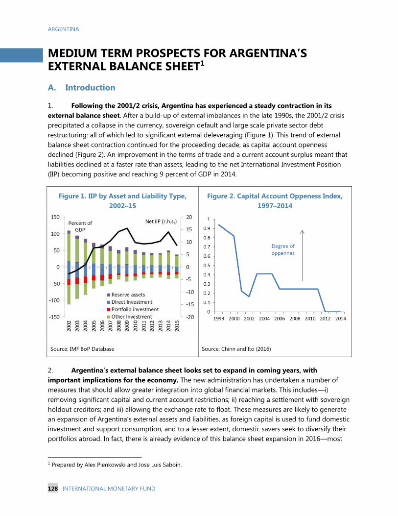
ARGENTINA


MEDIUM TERM PROSPECTS FOR ARGENTINA’S EXTERNAL BALANCE SHEET1

A. Introduction

1. Following the 2001/2 crisis, Argentina has experienced a steady contraction in its

external balance sheet. After a build-up of external imbalances in the late 1990s, the 2001/2 crisis

precipitated a collapse in the currency, sovereign default and large scale private sector debt

restructuring: all of which led to significant external deleveraging (Figure 1). This trend of external

balance sheet contraction continued for the proceeding decade, as capital account openness

declined (Figure 2). An improvement in the terms of trade and a current account surplus meant that

liabilities declined at a faster rate than assets, leading to the net International Investment Position

(IIP) becoming positive and reaching 9 percent of GDP in 2014.

Figure 1. IIP by Asset and Liability Type,

2002–15

Figure 2. Capital Account Oppeness Index,

1997–2014

Source: IMF BoP Database Source: Chinn and Ito (2016)

2. Argentina’s external balance sheet looks set to expand in coming years, with

important implications for the economy. The new administration has undertaken a number of

measures that should allow greater integration into global financial markets. This includes—i)

removing significant capital and current account restrictions; ii) reaching a settlement with sovereign

holdout creditors; and iii) allowing the exchange rate to float. These measures are likely to generate

an expansion of Argentina’s external assets and liabilities, as foreign capital is used to fund domestic

investment and support consumption, and to a lesser extent, domestic savers seek to diversify their

portfolios abroad. In fact, there is already evidence of this balance sheet expansion in 2016—most

1 Prepared by Alex Pienkowski and Jose Luis Saboin.

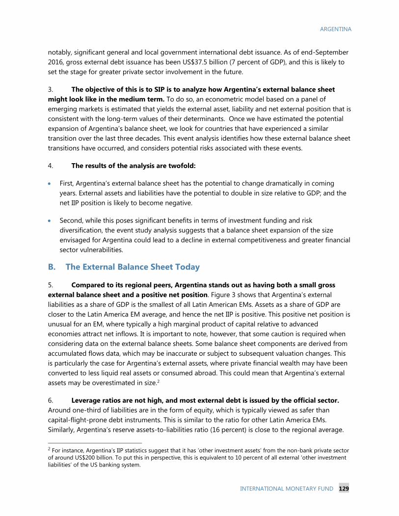
ARGENTINA


notably, significant general and local government international debt issuance. As of end-September

2016, gross external debt issuance has been US$37.5 billion (7 percent of GDP), and this is likely to

set the stage for greater private sector involvement in the future.

3. The objective of this is to SIP is to analyze how Argentina’s external balance sheet

might look like in the medium term. To do so, an econometric model based on a panel of

emerging markets is estimated that yields the external asset, liability and net external position that is

consistent with the long-term values of their determinants. Once we have estimated the potential

expansion of Argentina’s balance sheet, we look for countries that have experienced a similar

transition over the last three decades. This event analysis identifies how these external balance sheet

transitions have occurred, and considers potential risks associated with these events.

4. The results of the analysis are twofold:

First, Argentina’s external balance sheet has the potential to change dramatically in coming

years. External assets and liabilities have the potential to double in size relative to GDP; and the

net IIP position is likely to become negative.

Second, while this poses significant benefits in terms of investment funding and risk

diversification, the event study analysis suggests that a balance sheet expansion of the size

envisaged for Argentina could lead to a decline in external competitiveness and greater financial

sector vulnerabilities.

B. The External Balance Sheet Today

5. Compared to its regional peers, Argentina stands out as having both a small gross

external balance sheet and a positive net position. Figure 3 shows that Argentina’s external

liabilities as a share of GDP is the smallest of all Latin American EMs. Assets as a share of GDP are

closer to the Latin America EM average, and hence the net IIP is positive. This positive net position is

unusual for an EM, where typically a high marginal product of capital relative to advanced

economies attract net inflows. It is important to note, however, that some caution is required when

considering data on the external balance sheets. Some balance sheet components are derived from

accumulated flows data, which may be inaccurate or subject to subsequent valuation changes. This

is particularly the case for Argentina’s external assets, where private financial wealth may have been

converted to less liquid real assets or consumed abroad. This could mean that Argentina’s external

assets may be overestimated in size.2

6. Leverage ratios are not high, and most external debt is issued by the official sector.

Around one-third of liabilities are in the form of equity, which is typically viewed as safer than

capital-flight-prone debt instruments. This is similar to the ratio for other Latin America EMs.

Similarly, Argentina’s reserve assets-to-liabilities ratio (16 percent) is close to the regional average.

2 For instance, Argentina’s IIP statistics suggest that it has ‘other investment assets’ from the non-bank private sector

of around US$200 billion. To put this in perspective, this is equivalent to 10 percent of all external ‘other investment

liabilities’ of the US banking system.

ARGENTINA


Such leverage ratios, along with Argentina’s overall positive net IIP position, suggests that at present

the economy is not overly reliant on debt financing to fund investment and consumption. The

general government and central bank account for over 50 percent of external debt. In contrast, the

banking sector has borrowed very little from abroad, implying very little intermediation through the

banking sector. Part of this is due to strict regulatory controls imposed on the cross border

operations of banks, including limits on overall exposure. Instead, the non-bank private sector

seems to borrow directly from abroad (Figure 4). This borrowing is concentrated in the petroleum

and industrial manufacturing industries; and predominately associated with credit lines for import

financing. Given that the non-bank private sector makes up over 70 percent of GDP, its share of

overall external debt is relatively small.

Figure 3. IIP Relative to Regional Peers, 2014 Figure 4. Sectoral Breakdown of

External Debt, 2015Q2

Source: IMF BoP Database Source: Quarterly external debt database (SDDS)

7. The external balance sheet is robust to currency risk, but is more vulnerable to

liquidity risks. Estimates of the currency composition suggest that virtually all external assets and

liabilities are denominated in foreign currencies (Figure 5). Given the positive net IIP position, a

currency depreciation will, all things being equal, boost the net wealth of residents. This provides a

natural buffer to external shocks. There may, however, be currency mismatches within particular

sectors or agents within the economy, whereby exchange rate shocks could still cause balance sheet

problems that affect the real economy. In terms of maturity risks, around one-third of total external

debt is short-term.3 Furthermore, this short-term debt seems to be concentrated in the non-bank

private sector (Figure 6). This result is perhaps not surprising, given that such borrowing is often

associated with import financing. However, the reliance on this form of financing still has the

potential to increase liquidity risks for the non-bank private sector.

3 Defined as remaining maturity of one year or less.

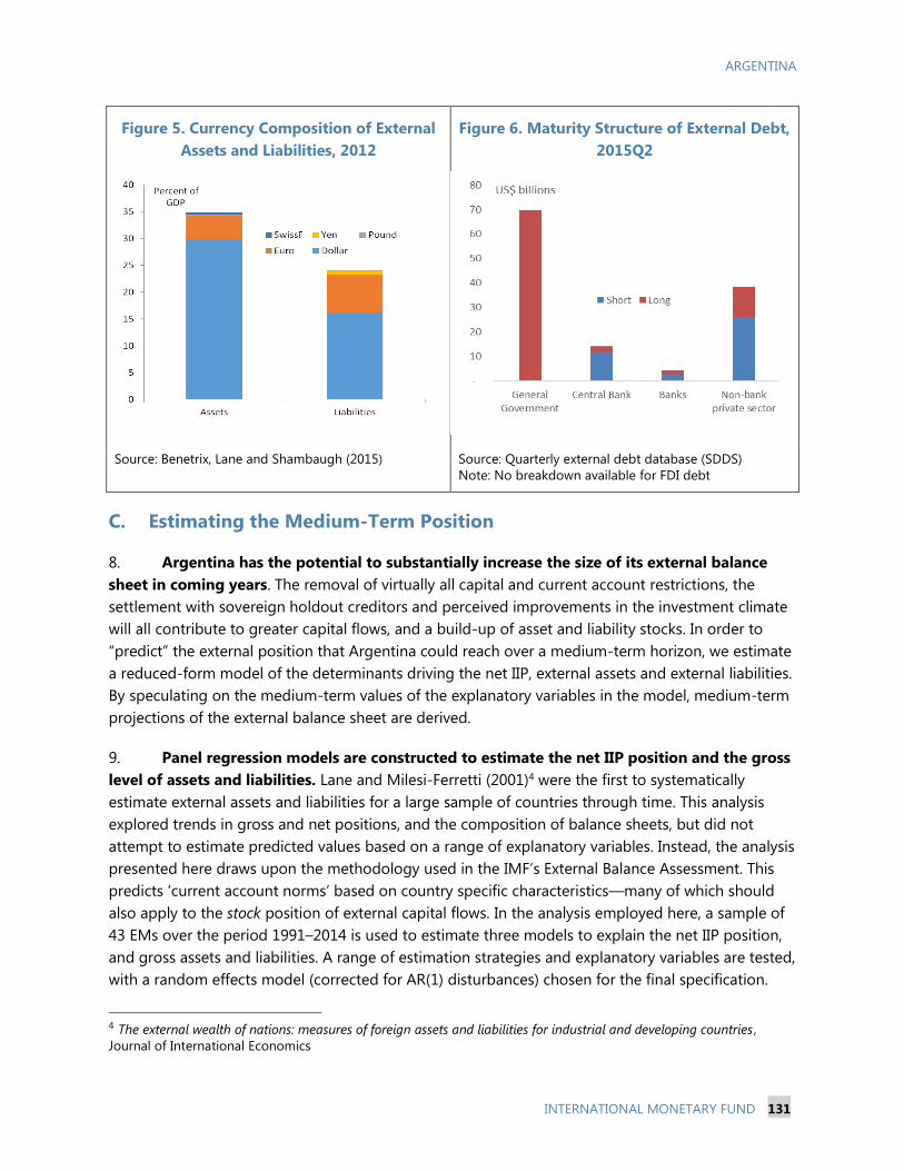
ARGENTINA


Figure 5. Currency Composition of External

Assets and Liabilities, 2012

Figure 6. Maturity Structure of External Debt,

2015Q2

Source: Benetrix, Lane and Shambaugh (2015) Source: Quarterly external debt database (SDDS)

Note: No breakdown available for FDI debt

C. Estimating the Medium-Term Position

8. Argentina has the potential to substantially increase the size of its external balance

sheet in coming years. The removal of virtually all capital and current account restrictions, the

settlement with sovereign holdout creditors and perceived improvements in the investment climate

will all contribute to greater capital flows, and a build-up of asset and liability stocks. In order to

“predict” the external position that Argentina could reach over a medium-term horizon, we estimate

a reduced-form model of the determinants driving the net IIP, external assets and external liabilities.

By speculating on the medium-term values of the explanatory variables in the model, medium-term

projections of the external balance sheet are derived.

9. Panel regression models are constructed to estimate the net IIP position and the gross

level of assets and liabilities. Lane and Milesi-Ferretti (2001)4 were the first to systematically

estimate external assets and liabilities for a large sample of countries through time. This analysis

explored trends in gross and net positions, and the composition of balance sheets, but did not

attempt to estimate predicted values based on a range of explanatory variables. Instead, the analysis

presented here draws upon the methodology used in the IMF’s External Balance Assessment. This

predicts ‘current account norms’ based on country specific characteristics—many of which should

also apply to the stock position of external capital flows. In the analysis employed here, a sample of

43 EMs over the period 1991–2014 is used to estimate three models to explain the net IIP position,

and gross assets and liabilities. A range of estimation strategies and explanatory variables are tested,

with a random effects model (corrected for AR(1) disturbances) chosen for the final specification.

4 The external wealth of nations: measures of foreign assets and liabilities for industrial and developing countries ,

Journal of International Economics

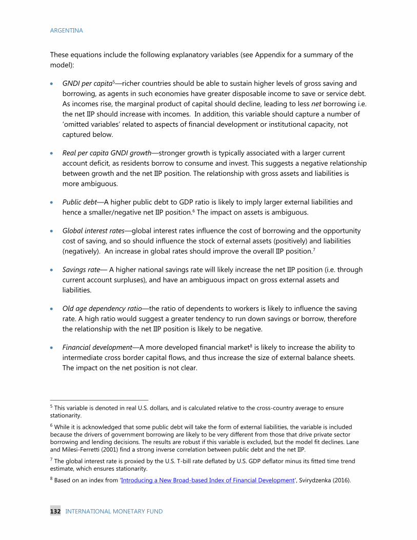
ARGENTINA


These equations include the following explanatory variables (see Appendix for a summary of the

model):

GNDI per capita5—richer countries should be able to sustain higher levels of gross saving and

borrowing, as agents in such economies have greater disposable income to save or service debt.

As incomes rise, the marginal product of capital should decline, leading to less net borrowing i.e.

the net IIP should increase with incomes. In addition, this variable should capture a number of

‘omitted variables’ related to aspects of financial development or institutional capacity, not

captured below.

Real per capita GNDI growth—stronger growth is typically associated with a larger current

account deficit, as residents borrow to consume and invest. This suggests a negative relationship

between growth and the net IIP position. The relationship with gross assets and liabilities is

more ambiguous.

Public debt—A higher public debt to GDP ratio is likely to imply larger external liabilities and

hence a smaller/negative net IIP position.6 The impact on assets is ambiguous.

Global interest rates—global interest rates influence the cost of borrowing and the opportunity

cost of saving, and so should influence the stock of external assets (positively) and liabilities

(negatively). An increase in global rates should improve the overall IIP position.7

Savings rate— A higher national savings rate will likely increase the net IIP position (i.e. through

current account surpluses), and have an ambiguous impact on gross external assets and

liabilities.

Old age dependency ratio—the ratio of dependents to workers is likely to influence the saving

rate. A high ratio would suggest a greater tendency to run down savings or borrow, therefore

the relationship with the net IIP position is likely to be negative.

Financial development—A more developed financial market8 is likely to increase the ability to

intermediate cross border capital flows, and thus increase the size of external balance sheets.

The impact on the net position is not clear.

5 This variable is denoted in real U.S. dollars, and is calculated relative to the cross-country average to ensure

stationarity.

6 While it is acknowledged that some public debt will take the form of external liabilities, the variable is included

because the drivers of government borrowing are likely to be very different from those that drive private sector

borrowing and lending decisions. The results are robust if this variable is excluded, but the model fit declines. Lane

and Milesi-Ferretti (2001) find a strong inverse correlation between public debt and the net IIP.

7 The global interest rate is proxied by the U.S. T-bill rate deflated by U.S. GDP deflator minus its fitted time trend

estimate, which ensures stationarity.

8 Based on an index from ‘Introducing a New Broad-based Index of Financial Development’, Svirydzenka (2016).

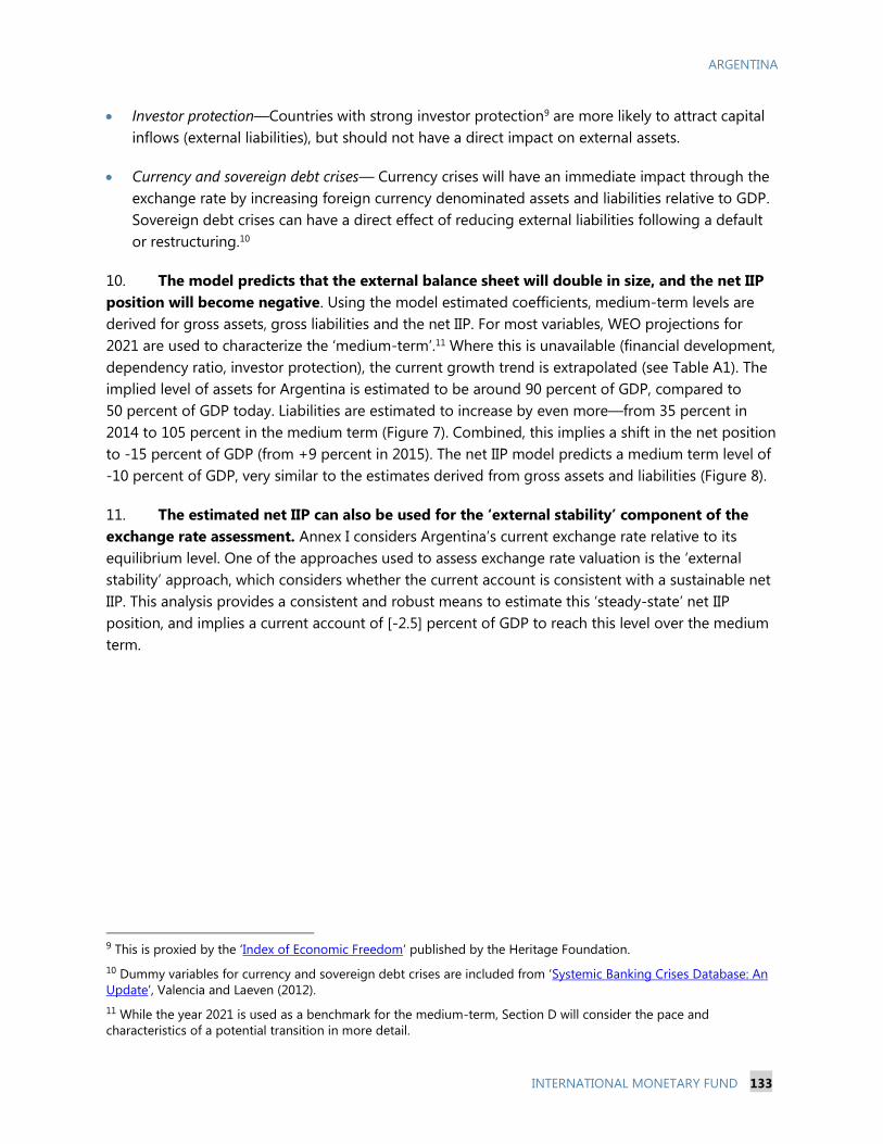
https://www.imf.org/external/pubs/ft/wp/2016/wp1605.pdf

ARGENTINA


Investor protection—Countries with strong investor protection9 are more likely to attract capital

inflows (external liabilities), but should not have a direct impact on external assets.

Currency and sovereign debt crises— Currency crises will have an immediate impact through the

exchange rate by increasing foreign currency denominated assets and liabilities relative to GDP.

Sovereign debt crises can have a direct effect of reducing external liabilities following a default

or restructuring.10

10. The model predicts that the external balance sheet will double in size, and the net IIP

position will become negative. Using the model estimated coefficients, medium-term levels are

derived for gross assets, gross liabilities and the net IIP. For most variables, WEO projections for

2021 are used to characterize the ‘medium-term’.11 Where this is unavailable (financial development,

dependency ratio, investor protection), the current growth trend is extrapolated (see Table A1). The

implied level of assets for Argentina is estimated to be around 90 percent of GDP, compared to

50 percent of GDP today. Liabilities are estimated to increase by even more—from 35 percent in

2014 to 105 percent in the medium term (Figure 7). Combined, this implies a shift in the net position

to -15 percent of GDP (from +9 percent in 2015). The net IIP model predicts a medium term level of

-10 percent of GDP, very similar to the estimates derived from gross assets and liabilities (Figure 8).

11. The estimated net IIP can also be used for the ‘external stability’ component of the

exchange rate assessment. Annex I considers Argentina’s current exchange rate relative to its

equilibrium level. One of the approaches used to assess exchange rate valuation is the ‘external

stability’ approach, which considers whether the current account is consistent with a sustainable net

IIP. This analysis provides a consistent and robust means to estimate this ‘steady-state’ net IIP

position, and implies a current account of [-2.5] percent of GDP to reach this level over the medium

term.

9 This is proxied by the ‘Index of Economic Freedom’ published by the Heritage Foundation.

10 Dummy variables for currency and sovereign debt crises are included from ‘Systemic Banking Crises Database: An

Update’, Valencia and Laeven (2012).

11 While the year 2021 is used as a benchmark for the medium-term, Section D will consider the pace and

characteristics of a potential transition in more detail.

http://www.heritage.org/index/

https://www.imf.org/external/pubs/cat/longres.aspx?sk=26015.0


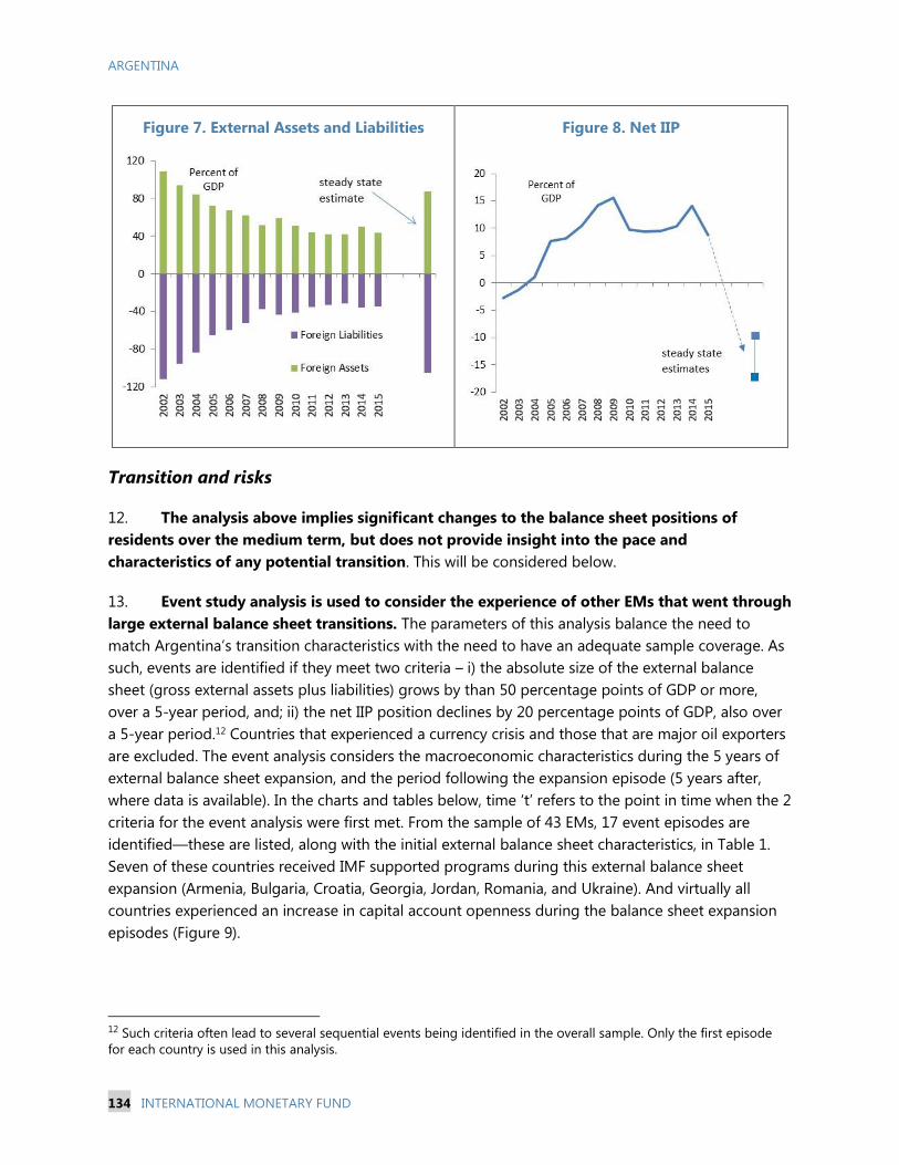
ARGENTINA


Figure 7. External Assets and Liabilities Figure 8. Net IIP

Transition and risks

12. The analysis above implies significant changes to the balance sheet positions of

residents over the medium term, but does not provide insight into the pace and

characteristics of any potential transition. This will be considered below.

13. Event study analysis is used to consider the experience of other EMs that went through

large external balance sheet transitions. The parameters of this analysis balance the need to

match Argentina’s transition characteristics with the need to have an adequate sample coverage. As

such, events are identified if they meet two criteria – i) the absolute size of the external balance

sheet (gross external assets plus liabilities) grows by than 50 percentage points of GDP or more,

over a 5-year period, and; ii) the net IIP position declines by 20 percentage points of GDP, also over

a 5-year period.12 Countries that experienced a currency crisis and those that are major oil exporters

are excluded. The event analysis considers the macroeconomic characteristics during the 5 years of

external balance sheet expansion, and the period following the expansion episode (5 years after,

where data is available). In the charts and tables below, time ‘t’ refers to the point in time when the 2

criteria for the event analysis were first met. From the sample of 43 EMs, 17 event episodes are

identified—these are listed, along with the initial external balance sheet characteristics, in Table 1.

Seven of these countries received IMF supported programs during this external balance sheet

expansion (Armenia, Bulgaria, Croatia, Georgia, Jordan, Romania, and Ukraine). And virtually all

countries experienced an increase in capital account openness during the balance sheet expansion

episodes (Figure 9).

12 Such criteria often lead to several sequential events being identified in the overall sample. Only the first episode

for each country is used in this analysis.

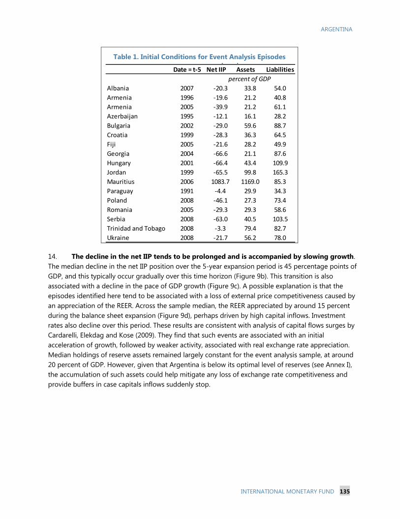
ARGENTINA


Table 1. Initial Conditions for Event Analysis Episodes

14. The decline in the net IIP tends to be prolonged and is accompanied by slowing growth.

The median decline in the net IIP position over the 5-year expansion period is 45 percentage points of

GDP, and this typically occur gradually over this time horizon (Figure 9b). This transition is also

associated with a decline in the pace of GDP growth (Figure 9c). A possible explanation is that the

episodes identified here tend to be associated with a loss of external price competitiveness caused by

an appreciation of the REER. Across the sample median, the REER appreciated by around 15 percent

during the balance sheet expansion (Figure 9d), perhaps driven by high capital inflows. Investment

rates also decline over this period. These results are consistent with analysis of capital flows surges by

Cardarelli, Elekdag and Kose (2009). They find that such events are associated with an initial

acceleration of growth, followed by weaker activity, associated with real exchange rate appreciation.

Median holdings of reserve assets remained largely constant for the event analysis sample, at around

20 percent of GDP. However, given that Argentina is below its optimal level of reserves (see Annex I),

the accumulation of such assets could help mitigate any loss of exchange rate competitiveness and

provide buffers in case capitals inflows suddenly stop.

Table 1: Initial conditions for event analysis episodes

Date = t-5 Net IIP Assets Liabilities

Albania 2007 -20.3 33.8 54.0

Armenia 1996 -19.6 21.2 40.8

Armenia 2005 -39.9 21.2 61.1

Azerbaijan 1995 -12.1 16.1 28.2

Bulgaria 2002 -29.0 59.6 88.7

Croatia 1999 -28.3 36.3 64.5

Fiji 2005 -21.6 28.2 49.9

Georgia 2004 -66.6 21.1 87.6

Hungary 2001 -66.4 43.4 109.9

Jordan 1999 -65.5 99.8 165.3

Mauritius 2006 1083.7 1169.0 85.3

Paraguay 1991 -4.4 29.9 34.3

Poland 2008 -46.1 27.3 73.4

Romania 2005 -29.3 29.3 58.6

Serbia 2008 -63.0 40.5 103.5

Trinidad and Tobago 2008 -3.3 79.4 82.7

Ukraine 2008 -21.7 56.2 78.0

percent of GDP

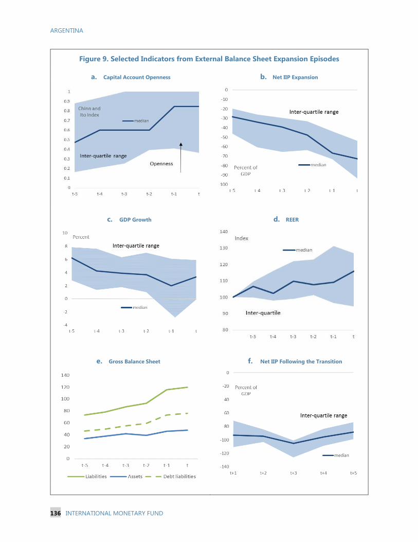
ARGENTINA


Figure 9. Selected Indicators from External Balance Sheet Expansion Episodes

a. Capital Account Openness b. Net IIP Expansion

c. GDP Growth d. REER

e. Gross Balance Sheet f. Net IIP Following the Transition

ARGENTINA


15. The expansion of external liabilities does not imply an overreliance on debt financing.

The median increase in external liabilities is 45 percentage points of GDP within the event analysis

sample, while assets grew by an average of 15 percentage points of GDP. Given the parameters of

event analysis, it is not surprising that liabilities grow at a faster pace than assets (Figure 9e).13 More

interesting, however, is that the proportion of debt as a share of overall liabilities remains very close

to the sample average (60 percent of total liabilities) during the entire balance sheet expansion

process i.e. equity finance expands at the same pace as debt accumulation. This suggests that

residents typically do not need to resort to excessive debt financing in order to access capital

markets during expansion episodes. Following the balance sheet expansion ‘event’, the growth of

assets and liabilities stabilizes, and the net IIP remains largely stable (Figure 9f).

16. The increase in liabilities during the expansion is largely driven by the private sector.

During these external balance sheet expansions episodes, average public-debt-to-GDP ratios

actually decline from around 47 to 41 percent of GDP, implying that this expansion was primarily

driven by the private sector. Perhaps not surprisingly, therefore, two countries subsequently

experienced banking crises (Hungary 2008 and Ukraine 2015) following the expansion—a much

higher incidence than the sample average (12 percent compared to 2 percent overall). A further

three countries received IMF supported packages during the subsequent two years (Armenia 2010,

Croatia 2004 and Romania 2011). Following these episodes, growth fell, liabilities increased and the

net IIP worsened (presumably due to valuation effects). The small sample size means that inferences

from this result need to be approached cautiously. However, Cardarelli et al (2009) find that around

one-third of capital inflow surges end in a ‘sudden stop’ or currency crisis. And it is clear that any

rapid expansion of external balance sheets, especially from a low base, poses risks to financial

stability.

D. Conclusion

17. After a decade of isolation from international capital markets, Argentina’s has a small

external balance sheet with few vulnerabilities. With the smallest external liability-to-GDP ratio of

all Latin American EMs and a positive net IIP, Argentina is broadly resilient to external shocks,

especially exchange rate risk. However, there may be pockets of vulnerability from short-term debt

in the non-bank private sector.

18. External assets and liabilities have the potential to grow substantially in coming years,

and the net position is likely to turn negative. Cross country panel regression analysis implies

that the external balance sheet has the potential change dramatically. Gross assets and liabilities

could more than double in size; and the net IIP position is likely to become negative.

19. The expansion is likely to be gradual, but dominated by the private sector, increasing

vulnerabilities in this area. Event study analysis suggests that this transition may occur at a gradual

pace, and does not need to be overly dependent on debt finance. However, the expansion is likely

13 When the event analysis parameters are solely determined by an expansion of the balance sheet (and not the

decline of the net IIP position), then the growth of assets and liabilities is broadly proportional.

ARGENTINA


to be driven by the private sector, which implies the need for vigilance in this sector. The authorities

should be particularly focused on an overly rapid expansion of the currently small banking sector,

which has little experience in intermediating international capital flows.

20. Policy considerations from this analysis include:

Is the concentration of short-term debt in the non-bank private sector a risk to the real

economy? As balance sheets grow, what prudential measures could be used to prevent liquidity

risks growing?

What measure can be taken to avoid an overvalued exchange rate as the net IIP position grows?

Potential policy measures include – i) reserve accumulation to lean against real appreciation and

build buffers; ii) fiscal consolidation to limit external financing and reduce crowding-out; iii)

supply side policies to improve non-price competitiveness.

How can the ‘right sort’ of capital flows be attracted? Given that long-term, local currency or

equity based finance provides for more resilient balance sheets, what policy can be pursued to

attract such inflows? Could measures (including capital controls) be needed to prevent riskier

inflows?

Is the banking sector ready to scale-up its external balance sheet? What prudential measures

could be used to ensure that banks are not overly exposed to currency and liquidity risks, whilst

allowing them to access international markets? What structural and institutional reforms can be

adopted to build long-term resilience to external shocks?

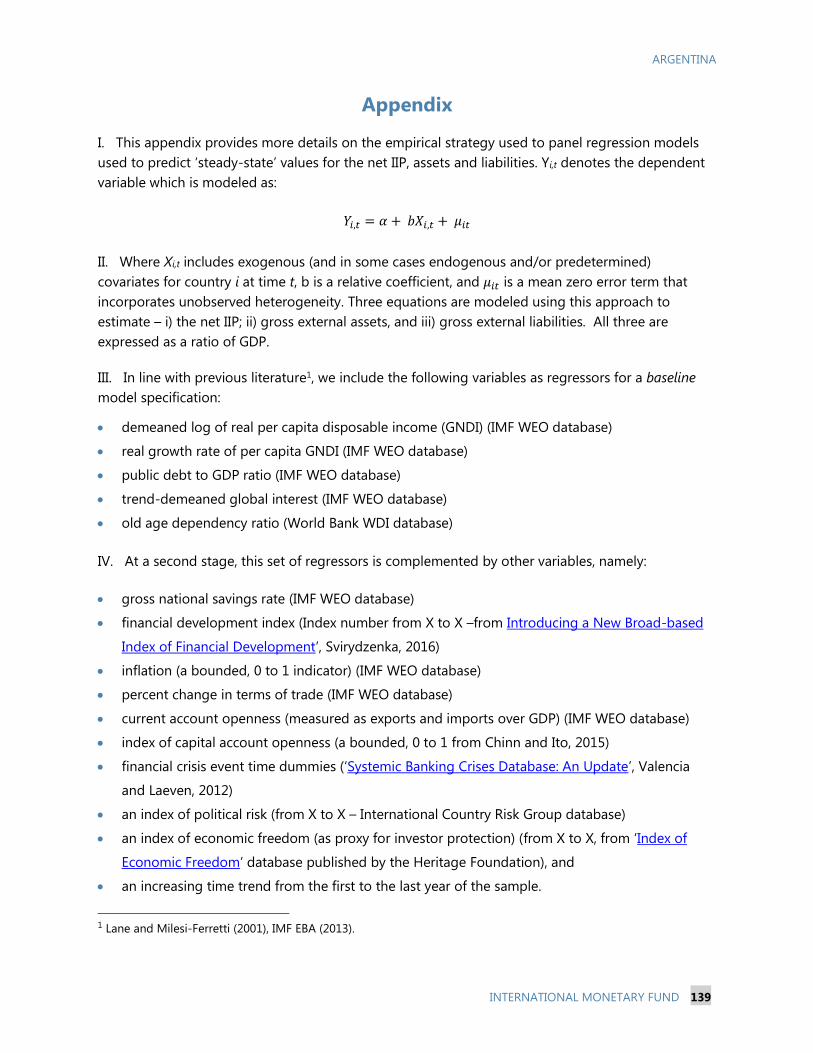
ARGENTINA


Appendix

I. This appendix provides more details on the empirical strategy used to panel regression models

used to predict ‘steady-state’ values for the net IIP, assets and liabilities. Yi,t denotes the dependent

variable which is modeled as:

𝑌𝑖,𝑡 = 𝛼 + 𝑏𝑋𝑖,𝑡 + 𝜇𝑖𝑡

II. Where Xi,t includes exogenous (and in some cases endogenous and/or predetermined)

covariates for country i at time t, b is a relative coefficient, and 𝜇𝑖𝑡 is a mean zero error term that

incorporates unobserved heterogeneity. Three equations are modeled using this approach to

estimate – i) the net IIP; ii) gross external assets, and iii) gross external liabilities. All three are

expressed as a ratio of GDP.

III. In line with previous literature1, we include the following variables as regressors for a baseline

model specification:

demeaned log of real per capita disposable income (GNDI) (IMF WEO database)

real growth rate of per capita GNDI (IMF WEO database)

public debt to GDP ratio (IMF WEO database)

trend-demeaned global interest (IMF WEO database)

old age dependency ratio (World Bank WDI database)

IV. At a second stage, this set of regressors is complemented by other variables, namely:

gross national savings rate (IMF WEO database)

financial development index (Index number from X to X –from Introducing a New Broad-based

Index of Financial Development’, Svirydzenka, 2016)

inflation (a bounded, 0 to 1 indicator) (IMF WEO database)

percent change in terms of trade (IMF WEO database)

current account openness (measured as exports and imports over GDP) (IMF WEO database)

index of capital account openness (a bounded, 0 to 1 from Chinn and Ito, 2015)

financial crisis event time dummies (‘Systemic Banking Crises Database: An Update’, Valencia

and Laeven, 2012)

an index of political risk (from X to X – International Country Risk Group database)

an index of economic freedom (as proxy for investor protection) (from X to X, from ‘Index of

Economic Freedom’ database published by the Heritage Foundation), and

an increasing time trend from the first to the last year of the sample.

1 Lane and Milesi-Ferretti (2001), IMF EBA (2013).






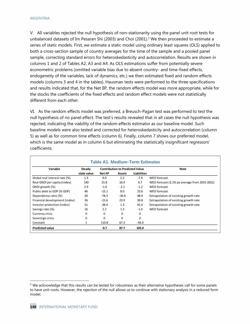
ARGENTINA


V. All variables rejected the null hypothesis of non-stationarity using the panel unit root tests for

unbalanced datasets of Im Pesaran Shi (2003) and Choi (2001).2 We then proceeded to estimate a

series of static models. First, we estimate a static model using ordinary least squares (OLS) applied to

both a cross-section sample of country averages for the time of the sample and a pooled panel

sample, correcting standard errors for heteroskedasticity and autocorrelation. Results are shown in

columns 1 and 2 of Tables A2, A3 and A4. As OLS estimations suffer from potentially severe

econometric problems (omitted variable bias due to absent country- and time-fixed effects,

endogeneity of the variables, lack of dynamics, etc.) we then estimated fixed and random effects

models (columns 3 and 4 in the tables). Hausman tests were performed to the three specifications

and results indicated that, for the Net IIP, the random effects model was more appropriate, while for

the stocks the coefficients of the fixed effects and random effect models were not statistically

different from each other.

VI. As the random effects model was preferred, a Breusch-Pagan test was performed to test the

null hypothesis of no panel effect. The test’s results revealed that in all cases the null hypothesis was

rejected, indicating the viability of the random effects estimator as our baseline model. Such

baseline models were also tested and corrected for heteroskedasticity and autocorrelation (column

5) as well as for common time effects (column 6). Finally, column 7 shows our preferred model,

which is the same model as in column 6 but eliminating the statistically insignificant regressors’

coefficients.

Table A1. Medium-Term Estimates

2 We acknowledge that this results can be tested for robustness as their alternative hypotheses call for some panels

to have unit roots. However, the rejection of the null allows us to continue with stationary analysis in a reduced form

model.

Table A1: Medium-Term Estimates

Net IIP Assets Liabilities

Global real interest rate (%) 1.3 9.9 2.2 -7.9 WEO forecast

Real GNDI per capita (index) 140 15.8 16.4 6.7 WEO forecast (2.1% pa average from 2015-2021)

GNDI growth (%) 2.9 -1.0 -2.1 -1.2 WEO forecast

Public debt to GDP (% GDP) 46 -15.1 8.0 23.6 WEO forecast

Dependency ratio (%) 20 -78.3 -30.6 48.0 Extrapolation of existing growth rate

Financial development (index) 36 -15.6 23.9 39.8 Extrapolation of existing growth rate

Investor protection (index) 51 -38.4 1.3 41.0 Extrapolation of existing growth rate

Savings rate (%) 16 2.2 1.3 -1.0 WEO forecast

Currency crisis 0 0 0 0

Sovereign crisis 0 0 0 0

Constant 1 110.8 67.3 -44.0

Predicted value -9.7 87.7 105.0

Contribution to Predicted ValueSteady

state value

Variable Note

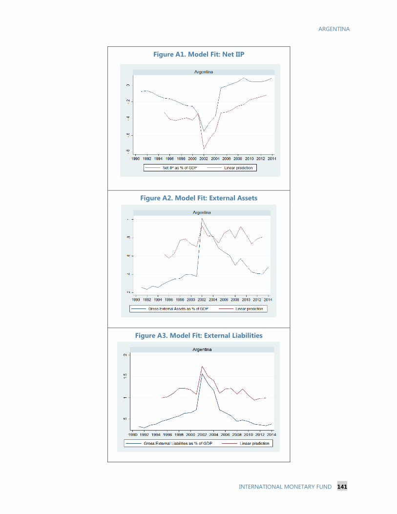
ARGENTINA


Figure A1. Model Fit: Net IIP

Figure A2. Model Fit: External Assets

Figure A3. Model Fit: External Liabilities

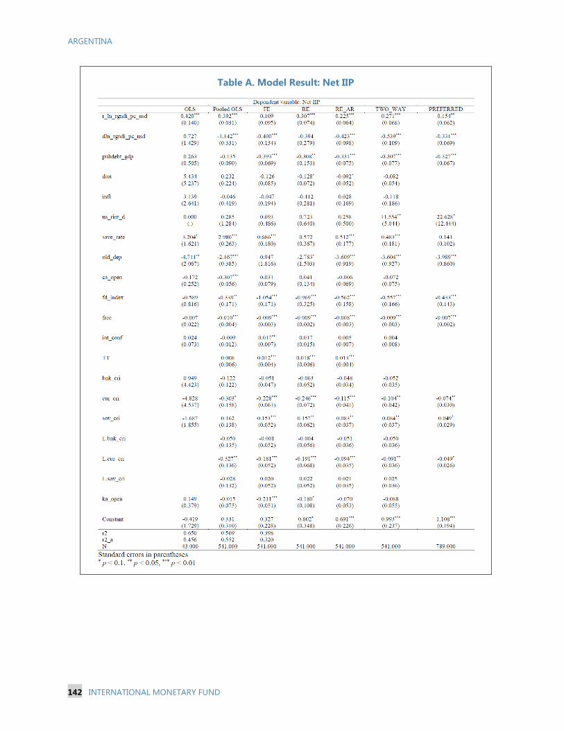
ARGENTINA


Table A. Model Result: Net IIP

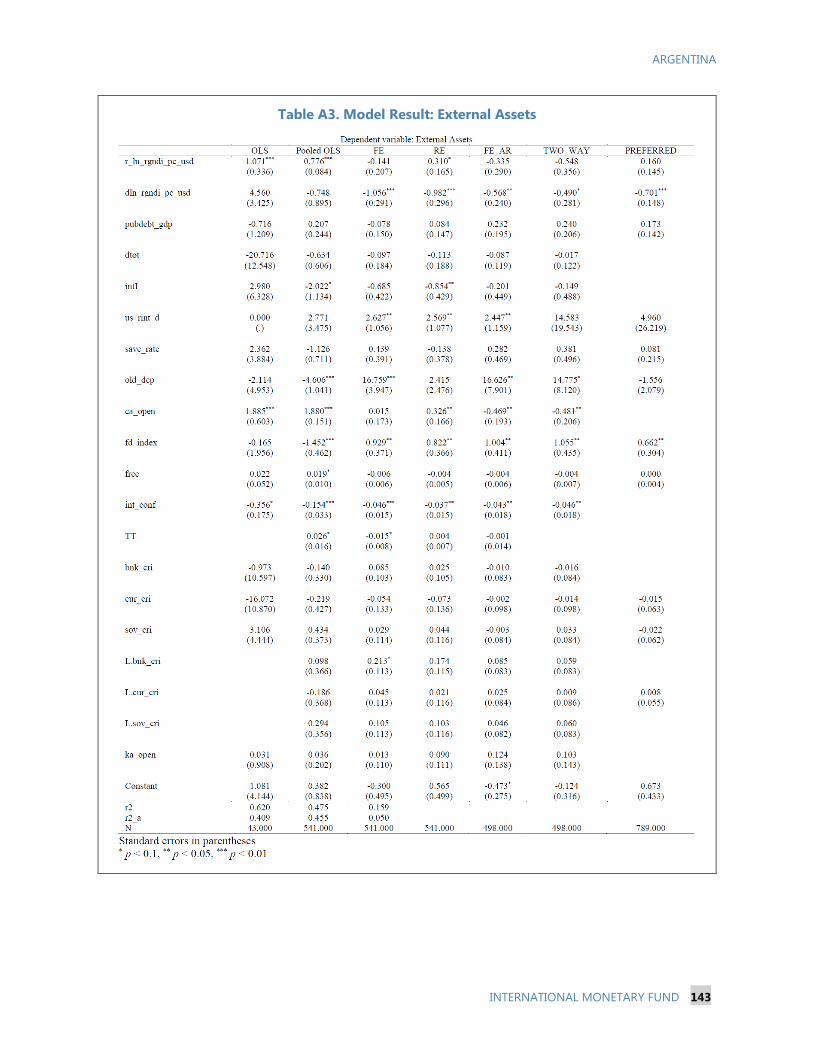
ARGENTINA


Table A3. Model Result: External Assets

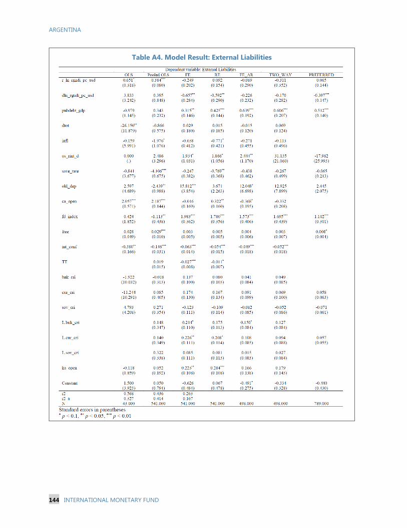
ARGENTINA


Table A4. Model Result: External Liabilities

Documents

IMF Country Report No. 16/347 ARGENTINA Country Report No. 16/347 ARGENTINA SELECTED ISSUES This Selected Issues paper on Argentina was prepared by a staff team of the International