Embed Size (px)
Citation preview
© International Monetary Fund
IMF Country Report No. 14/320
MEXICO SELECTED ISSUES
This Selected Issues Paper on Mexico was prepared by a staff team of the International Monetary Fund as background documentation for the periodic consultation with the member country. It is based on the information available at the time it was completed on October 23, 2014.
Copies of this report are available to the public from
International Monetary Fund Publication Services PO Box 92780 Washington, D.C. 20090
Telephone: (202) 623-7430 Fax: (202) 623-7201 E-mail: [email protected] Web: http://www.imf.org
Price: $18.00 per printed copy
International Monetary Fund Washington, D.C.
November 2014
MEXICO SELECTED ISSUES
Approved By Western Hemisphere
Department
Prepared By Phil de Imus, Fabian Valencia, Jorge Alvarez,
Jianping Zhou, Han Fei, and Jasmine Xiao
THE IMPACT OF MEXICO'S ENERGY REFORM ON HYDROCARBONS PRODUCTION _ 3
A. Current Challenges in the Energy Industry _____________________________________________ 3
B. Most Significant Reform Effort in 75 Years _____________________________________________ 4
C. Impact on Energy Production __________________________________________________________ 6
D. Resource Blessed ______________________________________________________________________ 6
E. How Long Does it Take?________________________________________________________________ 7
F. Production Scenarios ___________________________________________________________________ 8
G. How Much Investment and FDI? ______________________________________________________ 12
H. Natural Gas Imports and Transport ___________________________________________________ 14
I. Electricity Reform ______________________________________________________________________ 16
J. Conclusion _____________________________________________________________________________ 17
References _______________________________________________________________________________ 18
FIGURES
1. Illustrative Baseline Scenarios __________________________________________________________ 9
2. Illustrative Downside Scenarios _______________________________________________________ 11
MADE IN MEXICO: THE ENERGY REFORM AND MANUFACTURING OUTPUT _______19
A. Introduction __________________________________________________________________________ 19
B. The Mexican Manufacturing Sector Since NAFTA _____________________________________ 20
C. The Energy Reform: How Much of a Boost for Mexican Manufacturing? ______________ 22
D. Are There Additional Indirect Effects Through Spillovers? _____________________________ 26
E. Concluding Remarks and Policy Implications __________________________________________ 28
References _______________________________________________________________________________ 29
CONTENTS
October 23, 2014
MEXICO
2 INTERNATIONAL MONETARY FUND
TABLES
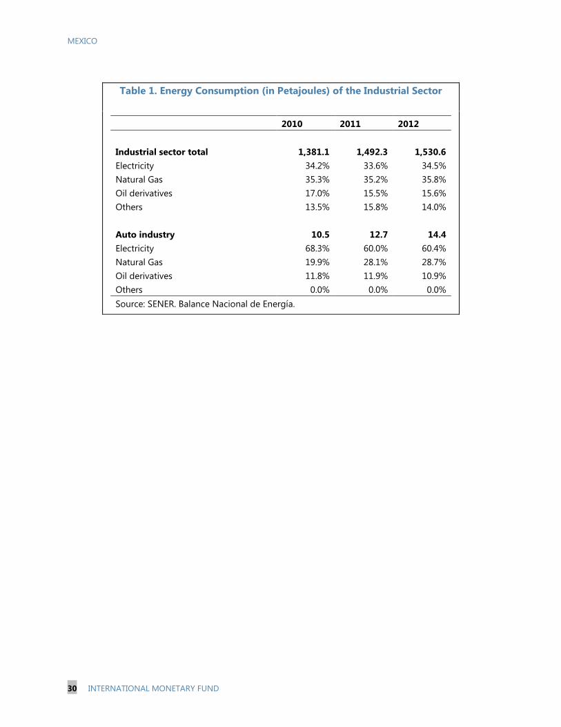
1. Energy Consumption (in Petajoules) of the Industrial Sector __________________________________ 30
2. Estimates of Elasticities of Manufacturing Output to Energy Prices. ___________________________ 31
3. Estimates of Elasticities When Energy Inputs Enter Separately _________________________________ 32
4. Differential Effects Across Subsectors _________________________________________________________ 33
APPENDIX
I. Panel VAR model ______________________________________________________________________________ 34
APPENDIX FIGURES
1. Impulse Response Functions to a Rise in Electricity Prices with Subsector Spillovers __________ 36
2. Impulse Response Functions to a Rise in Electricity Prices with Regional Spillovers ___________ 37
CAPITAL FLOW VOLATILITY AND INVESTOR BEHAVIOUR IN MEXICO ______________________38
A. Introduction ___________________________________________________________________________________ 38
B. Recent Episodes of Extreme Capital Movements in Mexico ___________________________________ 40
C. Behavior of Foreign and Domestic Mutual Funds in Mexico___________________________________ 43
D. Does Foreign Participation Amplify External Shock? A Time-Series Analysis of Mexican
Sovereign Bond Market __________________________________________________________________________ 48
E. Concluding Remarks __________________________________________________________________________ 52
References _______________________________________________________________________________________ 64
BOXES
1. OLS and Multivariate GARCH Models _________________________________________________________ 54
2. Data on Foreign Mutual Funds ________________________________________________________________ 55
FIGURES
1. Mexico: Extreme Capital Flow Episodes _______________________________________________________ 42
2. Evidence of Herding (net sellers as a percent of total funds) __________________________________ 45
3. Evidence of Herding (based on the herding index) ____________________________________________ 46
TABLES
1a. Bond Funds: Evidence of Positive Feedback Trading Behavior _______________________________ 56
1b. Equity Funds: Evidence of Positive Feedback Trading Behavior ______________________________ 57
2a. Robustness Check (1)—Using a Longer Sample for Foreign Mutual Funds ___________________ 58
2b. Robustness Check (2)—Using Dollar-Denominated Return on the 3-month Government
Bonds ____________________________________________________________________________________________ 59
3a. OLS Regression Results (VIX Shock) __________________________________________________________ 60
3b. OLS Regression Results (U.S. Tapering Shock) _______________________________________________ 61
4a. Multivariate GARCH Results (VIX Shock) _____________________________________________________ 62
4b. Multivariate GARCH Results (U.S. Tapering Shock) ___________________________________________ 63
MEXICO
INTERNATIONAL MONETARY FUND 3
THE IMPACT OF MEXICO'S ENERGY REFORM ON
HYDROCARBONS PRODUCTION1
1. The recently adopted energy reform could revolutionize Mexico’s hydrocarbons
sector. The reform aims to increase oil and gas production by eliminating the state oil company’s
(PEMEX) monopoly on exploration and production of hydrocarbons, while retaining the prime
directive that these resources are the property of the Mexican nation. Additionally, competition and
new regulatory structures are being implemented in midstream and downstream activities to
enhance the generation and distribution of natural gas and electricity to increase the efficiency of
service and reduce costs. Reducing electricity costs, in particular, could have a significant impact on
raising manufacturing output as discussed in a companion selected issues paper (SIP).2
2. This SIP will discuss the nature of these reforms and what problems these reforms are
addressing. It will then present illustrative production scenarios for crude oil and natural gas and
estimate the commensurate investment costs and foreign direct investment (FDI) associated with
each scenario. The paper also examines the markets for the distribution of natural gas and
electricity. It concludes with the key messages from our analysis.
A. Current Challenges in the Energy Industry3
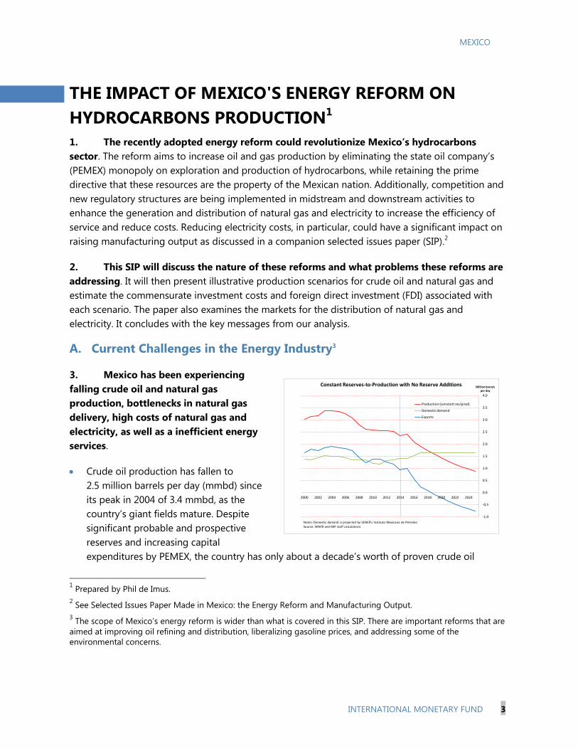
3. Mexico has been experiencing
falling crude oil and natural gas
production, bottlenecks in natural gas
delivery, high costs of natural gas and
electricity, as well as a inefficient energy
services.
Crude oil production has fallen to
2.5 million barrels per day (mmbd) since
its peak in 2004 of 3.4 mmbd, as the
country’s giant fields mature. Despite
significant probable and prospective
reserves and increasing capital
expenditures by PEMEX, the country has only about a decade’s worth of proven crude oil
1 Prepared by Phil de Imus.
2 See Selected Issues Paper Made in Mexico: the Energy Reform and Manufacturing Output.
3 The scope of Mexico’s energy reform is wider than what is covered in this SIP. There are important reforms that are
aimed at improving oil refining and distribution, liberalizing gasoline prices, and addressing some of the
environmental concerns.
-1.0
-0.5
0.0
0.5
1.0
1.5
2.0
2.5
3.0
3.5
4.0
2000 2002 2004 2006 2008 2010 2012 2014 2016 2018 2020 2022 2024
Million barrelsper day
Constant Reserves-to-Production with No Reserve Additions
Production (constant res/prod)
Domestic demand
Exports
Notes: Domestic demand is projected by SENER's Instituto Mexicano de Petroleo
Source: SENER and IMF staff calculations
MEXICO
4 INTERNATIONAL MONETARY FUND
reserves. PEMEX has had a difficult time fully replacing these reserves each year, achieving this
only twice in recent years. The yield from new fields has on the whole disappointed expectations,
and old fields are in their depletion phase. Without significant additions to proven reserves and
if the reserves-to-production ratio is held constant at the average of the last 5 years, production
would fall to about 1.5 mmbd and Mexico would turn into a net oil importer4 before the end of
the decade (see chart).
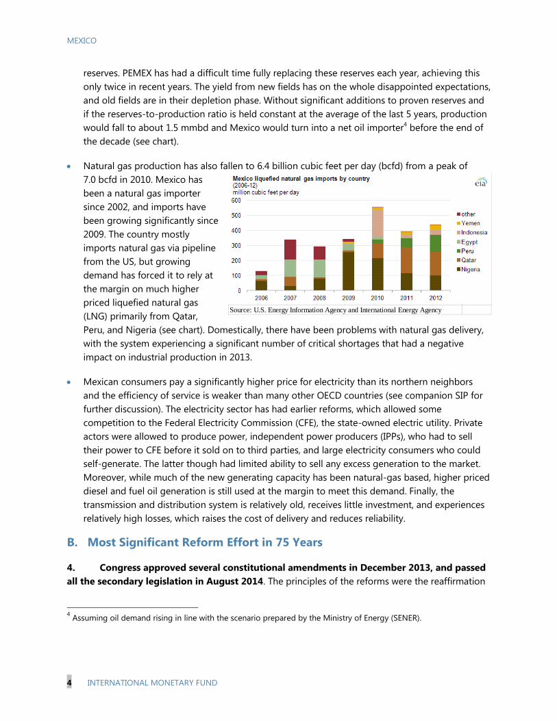
Natural gas production has also fallen to 6.4 billion cubic feet per day (bcfd) from a peak of
7.0 bcfd in 2010. Mexico has
been a natural gas importer
since 2002, and imports have
been growing significantly since
2009. The country mostly
imports natural gas via pipeline
from the US, but growing
demand has forced it to rely at
the margin on much higher
priced liquefied natural gas
(LNG) primarily from Qatar,
Peru, and Nigeria (see chart). Domestically, there have been problems with natural gas delivery,
with the system experiencing a significant number of critical shortages that had a negative
impact on industrial production in 2013.
Mexican consumers pay a significantly higher price for electricity than its northern neighbors
and the efficiency of service is weaker than many other OECD countries (see companion SIP for
further discussion). The electricity sector has had earlier reforms, which allowed some
competition to the Federal Electricity Commission (CFE), the state-owned electric utility. Private
actors were allowed to produce power, independent power producers (IPPs), who had to sell
their power to CFE before it sold on to third parties, and large electricity consumers who could
self-generate. The latter though had limited ability to sell any excess generation to the market.
Moreover, while much of the new generating capacity has been natural-gas based, higher priced
diesel and fuel oil generation is still used at the margin to meet this demand. Finally, the
transmission and distribution system is relatively old, receives little investment, and experiences
relatively high losses, which raises the cost of delivery and reduces reliability.
B. Most Significant Reform Effort in 75 Years
4. Congress approved several constitutional amendments in December 2013, and passed
all the secondary legislation in August 2014. The principles of the reforms were the reaffirmation
4 Assuming oil demand rising in line with the scenario prepared by the Ministry of Energy (SENER).
Source: US Energy Information Agency and International Energy Agency
Source: U.S. Energy Information Agency and International Energy Agency
MEXICO
INTERNATIONAL MONETARY FUND 5
that the nation owned the hydrocarbons in the ground; promotion of open and competitive markets
between state enterprises and private firms in both upstream, midstream, and downstream
operations; strengthening of the regulatory framework and institutions and the transformation of
Pemex and CFE; transparency and accountability of transactions; industrial safety; and the protection
of the environment and promotion of clear energy.5
5. These principles are carried out in practice by:
Opening up markets to competition. In mid-2014, the government completed the first round
of allocating Mexico’s oil fields (so-called “Round 0”), which assigned over 80 percent of
Mexico’s proven and probable oil reserves to PEMEX. In 2015, the government will begin to
auction the remaining exploration and production (E&P) blocks to state-owned and private
firms. The state will enter into a range of risk-sharing contracts with the winning bidders, which
include profit- and production-sharing as well as licenses. The flexibility in contracts makes it
likely that foreign firms will be willing to undertake the risk of exploration, while at the same
time providing incentives to ensure the state gets an appropriate share. The electric generation
market will be further opened up to allow independent power producers and firms that generate
their own electricity to sell directly to the market. Starting in 2018, domestic gasoline prices will
become fully market-determined, and PEMEX’s monoposony on gasoline imports will disappear.
Transformation of Pemex and CFE. Both state enterprises have been changed to state
productive enterprises, with greater autonomy in operations and budgeting. Gradually over
time, the fiscal take from PEMEX will be lowered to 65 percent as new fiscal regimes take hold
over the next 5 years. PEMEX will be allowed to enter into joint ventures and other contracts to
develop fields it received in Round 0. CFE will be allowed to contract with private parties for
natural gas supply and for investment and operations of transmission and distribution projects.
Strengthening of the regulatory framework. The role of the Ministry of Energy (SENER) and
the National Hydrocarbons Commission (CNH) are enhanced, so that new E&P contracts will be
agreed with the federal government and not PEMEX. Transparent auctions will be conducted by
CNH, and it will manage the contracts. Independent system operators, National Center for
Energy Control (CENACE) and National Center for Control of Natural Gas (CENEGAS), are created
to improve the efficiency of natural gas and electricity distribution and reduce potential conflicts
of interest. The Energy Regulatory Commission (CRE) will set tariffs for transmission, distribution,
and ancillary services.
A domestic content rule. Both assignments to PEMEX and other contracts will have domestic
content rules that gradually rise to 35 percent by 2025. There is also a minimum participation
5 The focus of this SIP is on the former four principles. It does not examine issues of environmental protection and
industrial safety. Important reforms were enacted here, including the creation of a new regulatory agency.
MEXICO
6 INTERNATIONAL MONETARY FUND
rule of 20 percent for PEMEX in deep water trans-boundary projects in order for it to gain the
know-how in that arena.
A new, independent sovereign wealth fund. The Mexican Oil Stabilization Fund, managed by
the central bank, has been created to administer the proceeds and payments from assignments
and contracts. This aims to increase transparency and could allow the government to save more
of its oil revenues.
C. Impact on Energy Production
6. We present baseline and downside scenarios for crude oil and natural gas production
for illustrative purposes only. The assumptions used were culled from discussions with and
documents from the relevant Mexican authorities, academics, and analysts from the private sector.
7. We approach the analysis by asking the following questions. Are there enough potential
reserves given the current geological estimates? What is the timeline for production given the type
of production, i.e. conventional, enhanced recovery, deepwater or shale? What would particular
targets for production imply for the proven reserve replacement ratios (RRRs) 1over time, and how
do those RRRs compare to historical trends. Additionally, how much would it cost to attain these
RRRs, and given assumptions for the domestic content rules, how much FDI could the projects
attract?
D. Resource Blessed
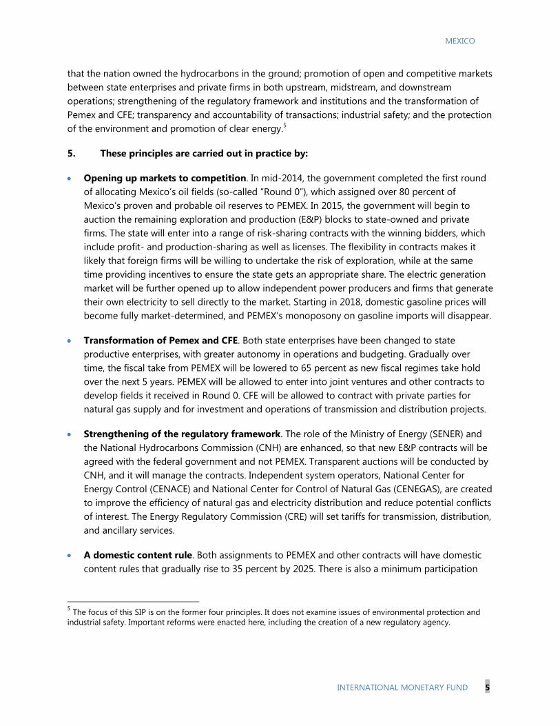
8. According to PEMEX’s statistics, crude oil and natural gas reserves are substantial.
Proven reserves, which are estimated to be
extractable with at least 90 percent
probability, amount to 10 billion barrels
(bbl) of crude oil and 13.6 trillion cubic feet
(tcf) of natural gas. Possible and probable
reserves, those estimated to be extractable
with a probability of 50 to 90 percent and
10 to 50 percent respectively, are reported
to be 21 bbl and 38.5 tcf (see chart). These
resources represent those in the current
fields that have been explored and are
being produced by Pemex as of end-2013.
1 The proven RRR is a key statistic which indicates how much of the production in a year is replaced by additions to
proven reserves. For example, a 100 percent RRR means that given 1 barrel in production, the energy company is
able to find 1 new barrel of oil in proven reserves. This would keep the level of proven reserves at a constant level.
0
10
20
30
40
50
60
70
80
90
100
Billion barrel of oil equivalentMexico's Reserves Potential
Possible 10%
Probable 50%
Proven 90%
Conventional
Deepwater
potential
Shale
potential
Potential additions
to proven reserves
Current proven
reserves
Source: Pemex
MEXICO
INTERNATIONAL MONETARY FUND 7
9. Deepwater and shale could yield sizeable new reserves, but more exploratory drilling
is required to more accurately measure the amounts. According to PEMEX, there is an estimated
27.1 billion barrels of oil equivalent (bboe) in the deep water Gulf of Mexico (GoM) and 60.2 bboe in
shale deposits in the northern part of the country. The U.S. Energy Information Agency ranks Mexico
8th among countries with 13 bbl of technically recoverable shale oil resources and 6th with 545 tcf
of technically recoverable natural gas. However, the number of exploratory wells in deepwater and
shale are relatively small compared to those in the U.S. side of the GoM, the deepwaters of Brazil,
and the shale fields in Eagle Ford Texas, so more information is need to ascertain the amounts.
E. How Long Does it Take?
10. The process of passing the constitutional reform and secondary laws are now
complete, as well the Round 0 assignment of fields to PEMEX. The immediate next step is to
implement Round 1 of bidding for the fields that were not assigned to Pemex. It is crucial that the
process in this round goes relatively smoothly and is perceived to be transparent to maintain
investor and political confidence in the reform. The bidding process is expected to be completed by
the second half of next year. Additionally, important regulatory changes are taking place that cover
exploration and production, as well as the distribution of both natural gas and electricity.
11. Over the next few years, improvements to production are more likely to come from
developing conventional fields, and secondary and enhanced recovery from existing,
producing fields. The government will likely have to rely on these sources from both PEMEX and
new entrants to meet its goal of increasing crude oil production to 3.0 mmbd by 2019.1 These
projects will take less time than unconventional sources given relatively faster processes, less
complexity, and PEMEX’s enhanced ability to contract with private firms, including farmouts,2 to
share investment costs or to import advanced technologies. Authorities indicated that about
70 percent of the blocks in the Round 1 auction will be those that are already probable reserves (2P)
that are more ready to become proven reserves and for extraction.
1 The government’s 3.0 mmbd production expectations had to be changed to 2019 due to an unexpected decline in
Pemex’s production in 2013.
2 Farmouts are E&P projects in which PEMEX contracts with a third party to perform all or parts of a project in blocks
assigned to PEMEX in Round 0.
MEXICO
8 INTERNATIONAL MONETARY FUND
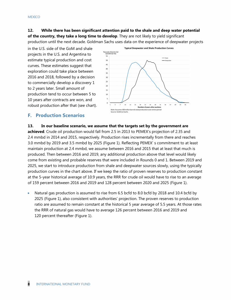
12. While there has been significant attention paid to the shale and deep water potential
of the country, they take a long time to develop. They are not likely to yield significant
production until the next decade. Goldman Sachs uses data on the experience of deepwater projects
in the U.S. side of the GoM and shale
projects in the U.S. and Argentina to
estimate typical production and cost
curves. These estimates suggest that
exploration could take place between
2016 and 2018, followed by a decision
to commercially develop a discovery 1
to 2 years later. Small amount of
production tend to occur between 5 to
10 years after contracts are won, and
robust production after that (see chart).
F. Production Scenarios
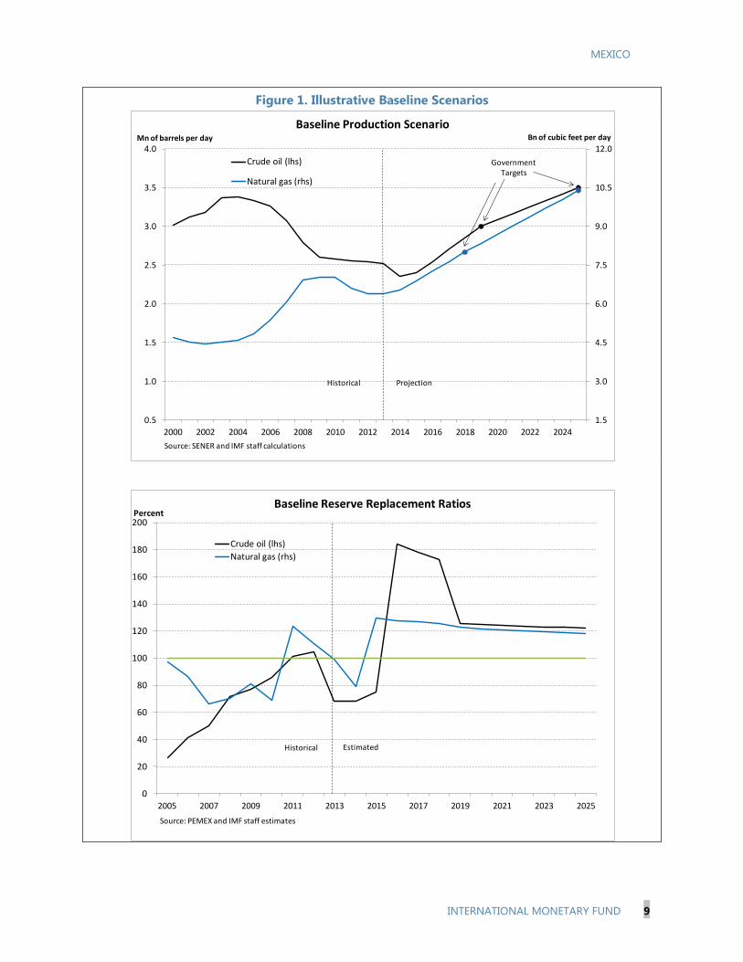
13. In our baseline scenario, we assume that the targets set by the government are
achieved. Crude oil production would fall from 2.5 in 2013 to PEMEX’s projection of 2.35 and
2.4 mmbd in 2014 and 2015, respectively. Production rises incrementally from there and reaches
3.0 mmbd by 2019 and 3.5 mmbd by 2025 (Figure 1). Reflecting PEMEX’ s commitment to at least
maintain production at 2.4 mmbd, we assume between 2016 and 2015 that at least that much is
produced. Then between 2016 and 2019, any additional production above that level would likely
come from existing and probable reserves that were included in Rounds 0 and 1. Between 2019 and
2025, we start to introduce production from shale and deepwater sources slowly, using the typically
production curves in the chart above. If we keep the ratio of proven reserves to production constant
at the 5-year historical average of 10.9 years, the RRR for crude oil would have to rise to an average
of 159 percent between 2016 and 2019 and 128 percent between 2020 and 2025 (Figure 1).
Natural gas production is assumed to rise from 6.5 bcfd to 8.0 bcfd by 2018 and 10.4 bcfd by
2025 (Figure 1), also consistent with authorities’ projection. The proven reserves to production
ratio are assumed to remain constant at the historical 5 year average of 5.5 years. At those rates
the RRR of natural gas would have to average 126 percent between 2016 and 2019 and
120 percent thereafter (Figure 1).
0
5
10
15
20
25
30
35
40
45
50
55
1 4 7 10 13 16 19 22 25 28 31 34 37 40 43 46
Thousands of barrels of oil equivalent per day
Number of years after auctions
Typical Deepwater and Shale Production Curves
Shale
Deepwater
Note: Assumes 300 millon barrels total production over entire periodSource: Goldman Sachs
MEXICO
INTERNATIONAL MONETARY FUND 9
Figure 1. Illustrative Baseline Scenarios
1.5
3.0
4.5
6.0
7.5
9.0
10.5
12.0
0.5
1.0
1.5
2.0
2.5
3.0
3.5
4.0
2000 2002 2004 2006 2008 2010 2012 2014 2016 2018 2020 2022 2024
Bn of cubic feet per dayMn of barrels per day
Baseline Production Scenario
Crude oil (lhs)
Natural gas (rhs)
Historical Projection
Source: SENER and IMF staff calculations
Government Targets
0
20
40
60
80
100
120
140
160
180
200
2005 2007 2009 2011 2013 2015 2017 2019 2021 2023 2025
PercentBaseline Reserve Replacement Ratios
Crude oil (lhs)
Natural gas (rhs)
Historical Estimated
Source: PEMEX and IMF staff estimates
MEXICO
10 INTERNATIONAL MONETARY FUND
14. Between 2015 and 2019, additions to proven reserves will likely come from the
existing fields and 2P reserves, which can be produced by Pemex and its partners or new
entrants. The oil is likely to come from conventional fields and the application of secondary and
enhanced recovery techniques on existing fields. Between 2020 and 2025, shale and deep water
sources are likely to come into play that are developed and produced by firms winning fields from
federal government auctions.
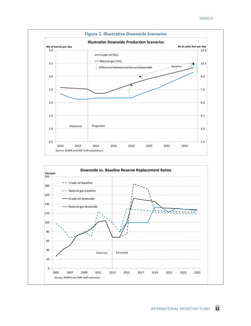
15. We construct a downside scenario which assumes the government’s production goals
are not met as scheduled. First, we assume that Pemex production in 2015 stays at the 2014
projected level of 2.35 mmbd, and this level continues between 2016 and 2025. From 2016 to 2019,
any additional production above 2.35 mmbd is assumed to come from half of the 2P reserves in the
Round 1 blocks announced on August 13, 2014 spread over the 4 years. Production does increase
over this time, but only reaches 2.82 mmbd by 2019. From 2020 to 2025, other sources including
conventional, shale, and deepwater contribute to production, with the latter two following the
typically production schedule shown in Figure 4. Production rises to 3.33 mmbd by 2025 (Figure 2).
We also assume that the proven reserves to production ratio stays constant at the historical 5 year
average of 10.9 years. The scenario is equivalent to the government achieving its production golas,
but with a delay of 2 years, i.e. 3.0 mmbd in 2021 vs. 2019 and 3.5 mmbd in 2027 vs. 2025. Under
this scenario, the RRR for crude oil would have to average 149 percent between 2015 and 2019 and
then increase to an average of 130 percent from 2019 to 2025 (Figure 2).
Under a downside scenario, we assume natural gas production stays constant at the projected
2014 level of 6.5 bcfd between 2015 and 2018. This means no additions to production in the first
few years, and effectively means that any additions to proven reserves over this time are only in
crude oil not natural gas. Natural gas production only increases from 2019 to 2025, reaching
9.5 bcfd in the last year. Shale gas only contributes to production starting in 2021, consistent
with the longer end of the 5 to 10 year range between auction and the start of production. The
proven reserves to production ratio for gas are assumed to remain constant at the historical 5-
year average of 5.5 years. In this scenario, the government’s goal of 8.0 bcfd is only reached
after 2021 and 10.4 bcfd in 2027 (Figure 2). The RRR of natural gas under this scenario would
have to be 100 percent in the first period and 129 percent in the latter (Figure 2).
MEXICO
INTERNATIONAL MONETARY FUND 11
Figure 2. Illustrative Downside Scenarios
1.5
3.0
4.5
6.0
7.5
9.0
10.5
12.0
0.5
1.0
1.5
2.0
2.5
3.0
3.5
4.0
2010 2012 2014 2016 2018 2020 2022 2024
Bn of cubic feet per dayMn of barrels per day
Illustrative Downside Production Scenarios
Crude oil (lhs)
Natural gas (rhs)
Baseline
Historical Projection
Source: SENER and IMF staff calculations
Difference between basline and downside
0
20
40
60
80
100
120
140
160
180
200
2005 2007 2009 2011 2013 2015 2017 2019 2021 2023 2025
PercentDownside vs. Baseline Reserve Replacement Ratios
Crude oil baseline
Natural gas baseline
Crude oil downside
Natural gas downside
Historical Estimated
Source: PEMEX and IMF staff estimates
MEXICO
12 INTERNATIONAL MONETARY FUND
G. How Much Investment and FDI?
16. In order to estimate the amount of investment needed annually to achieve the higher
RRRs, we need the amount of addition to reserves each year implied by the new RRRs, and a
cost per barrel of crude oil or per million cubic feet per day of natural gas to develop the
different types of projects.
For the exploration of new
conventional fields, the cost of finding
crude oil and natural gas is about $20
per barrel according to the EIA in
South America and the U.S.1 Projects
that used advanced recovery
techniques to extract more oil or gas
from existing fields cost between 15 to
25 dollars per barrel, according to
discussions with industry analysts. We
assume that cost for these two types of
projects is the same for crude oil and
natural gas, which is particularly true for associated natural gas—gas found in field where oil is
also found.
For shale and deep water projects, we use cost curves provided by Goldman Sachs (see chart
above). Their energy industry researchers used historical cost data from existing projects (like
Eagle Ford in the U.S. and deep water fields in Brazil) to estimate the average cost of a typical
project. The cost of shale development is about $11 to $20 per boe on average and deep water
development at $9 to $20 per boe. We use Goldman’s estimated cost curves in our analysis
which better captures the timing of capital expenditures.
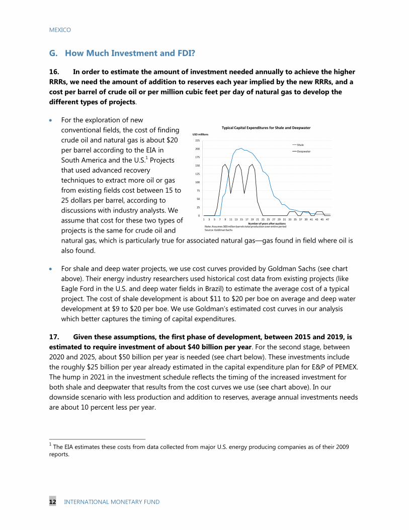
17. Given these assumptions, the first phase of development, between 2015 and 2019, is
estimated to require investment of about $40 billion per year. For the second stage, between
2020 and 2025, about $50 billion per year is needed (see chart below). These investments include
the roughly $25 billion per year already estimated in the capital expenditure plan for E&P of PEMEX.
The hump in 2021 in the investment schedule reflects the timing of the increased investment for
both shale and deepwater that results from the cost curves we use (see chart above). In our
downside scenario with less production and addition to reserves, average annual investments needs
are about 10 percent less per year.
1 The EIA estimates these costs from data collected from major U.S. energy producing companies as of their 2009
reports.
0
25
50
75
100
125
150
175
200
225
1 3 5 7 9 11 13 15 17 19 21 23 25 27 29 31 33 35 37 39 41 43 45 47
USD milllions
Number of years after auctions
Typical Capital Expenditures for Shale and Deepwater
Shale
Deepwater
Note: Assumes 300 millon barrels total production over entire periodSource: Goldman Sachs
MEXICO
INTERNATIONAL MONETARY FUND 13
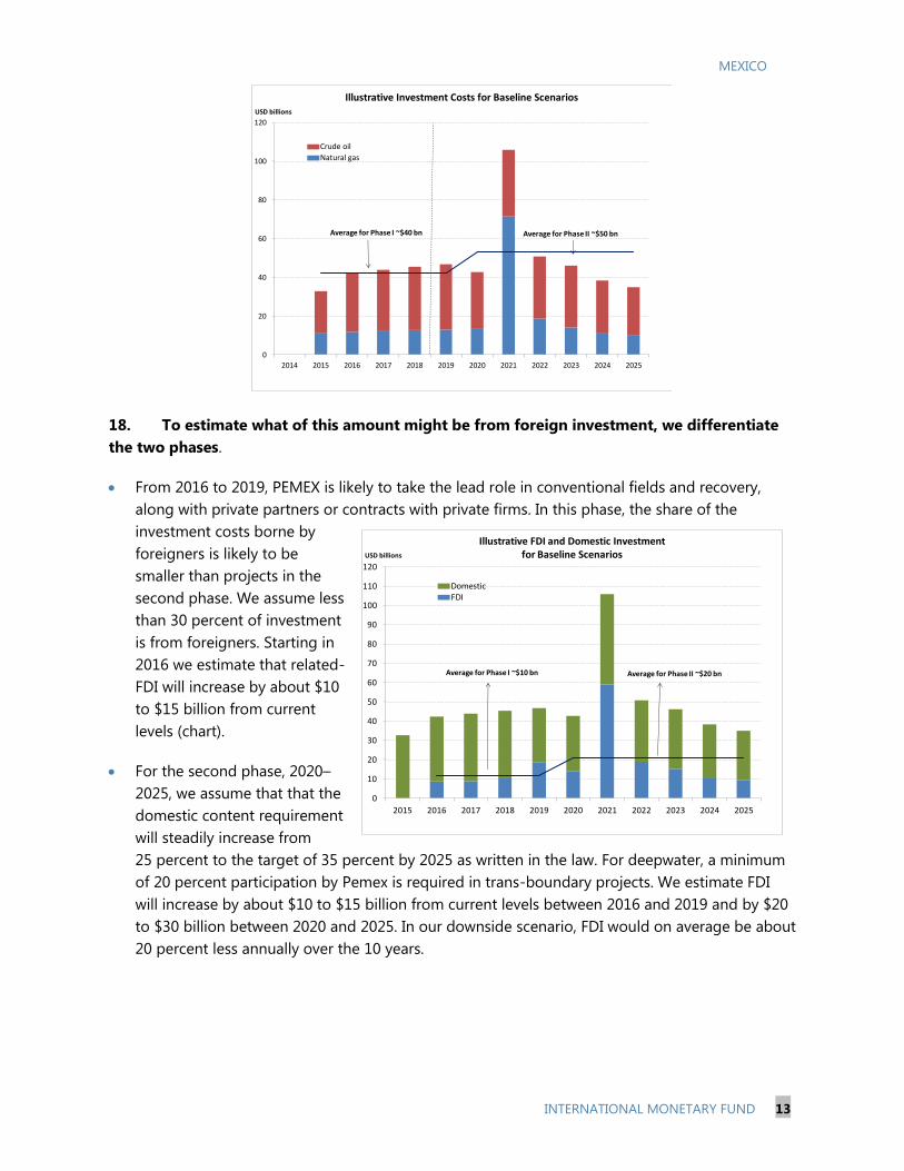
18. To estimate what of this amount might be from foreign investment, we differentiate
the two phases.
From 2016 to 2019, PEMEX is likely to take the lead role in conventional fields and recovery,
along with private partners or contracts with private firms. In this phase, the share of the
investment costs borne by
foreigners is likely to be
smaller than projects in the
second phase. We assume less
than 30 percent of investment
is from foreigners. Starting in
2016 we estimate that related-
FDI will increase by about $10
to $15 billion from current
levels (chart).
For the second phase, 2020–
2025, we assume that that the
domestic content requirement
will steadily increase from
25 percent to the target of 35 percent by 2025 as written in the law. For deepwater, a minimum
of 20 percent participation by Pemex is required in trans-boundary projects. We estimate FDI
will increase by about $10 to $15 billion from current levels between 2016 and 2019 and by $20
to $30 billion between 2020 and 2025. In our downside scenario, FDI would on average be about
20 percent less annually over the 10 years.
0
20
40
60
80
100
120
2014 2015 2016 2017 2018 2019 2020 2021 2022 2023 2024 2025
USD billions
Illustrative Investment Costs for Baseline Scenarios
Crude oil
Natural gas
Average for Phase I ~$40 bn Average for Phase II ~$50 bn
0
10
20
30
40
50
60
70
80
90
100
110
120
2015 2016 2017 2018 2019 2020 2021 2022 2023 2024 2025
USD billions
Illustrative FDI and Domestic Investment for Baseline Scenarios
DomesticFDI
Average for Phase I ~$10 bn Average for Phase II ~$20 bn
MEXICO
14 INTERNATIONAL MONETARY FUND
19. In order to compare our results, there is a wide range of analysts’ estimates of the
amount of investment and FDI that could result from the energy reform (see table). These
estimates come from industry experts and surveys of interest in participation in projects. They range
from a low of less than US$10 billion per year to a high of US$30 billion or more. Our estimates are
more in line with the lower end of those ranges. Take note that we only estimate investments into
the development of oil and natural gas fields, and do not account for the wider scope of the energy
reform. Some analysts have considered the broader scope of the reform.
H. Natural Gas Imports and Transport
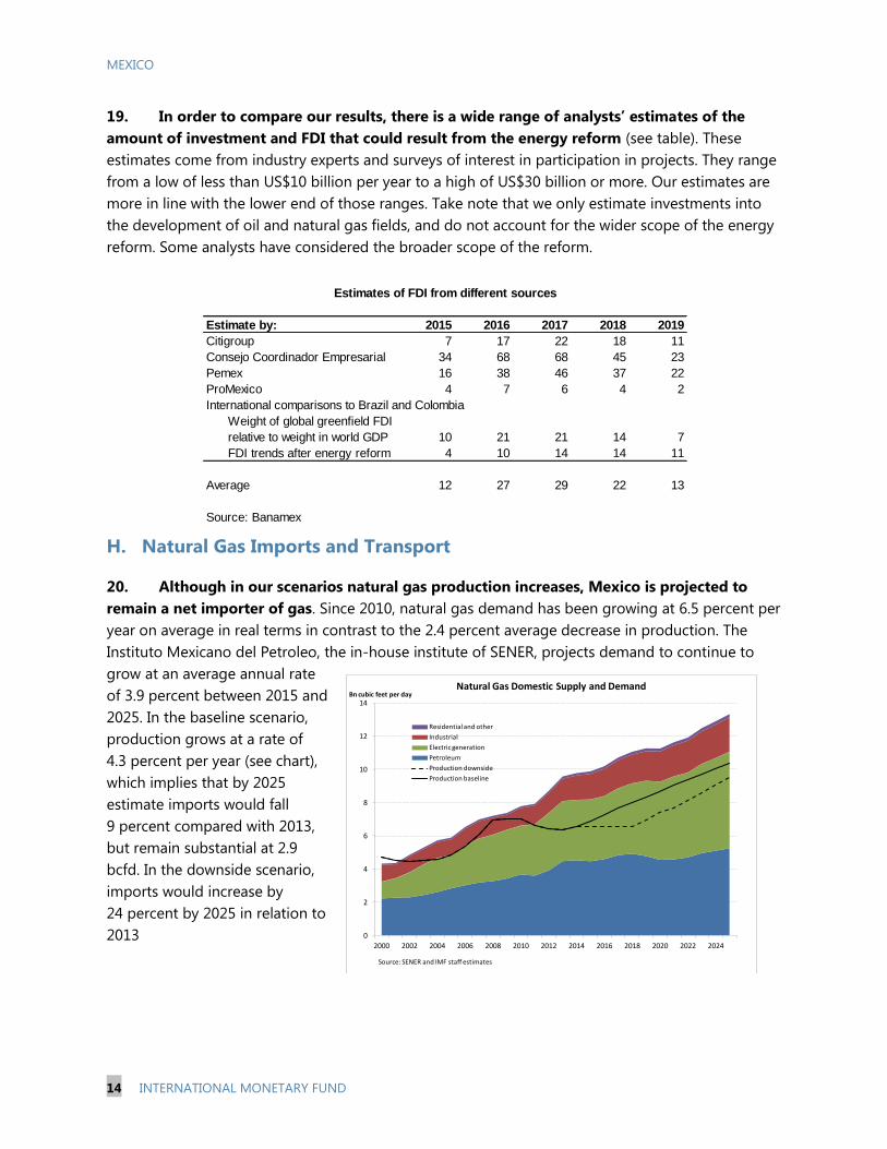
20. Although in our scenarios natural gas production increases, Mexico is projected to
remain a net importer of gas. Since 2010, natural gas demand has been growing at 6.5 percent per
year on average in real terms in contrast to the 2.4 percent average decrease in production. The
Instituto Mexicano del Petroleo, the in-house institute of SENER, projects demand to continue to
grow at an average annual rate
of 3.9 percent between 2015 and
2025. In the baseline scenario,
production grows at a rate of
4.3 percent per year (see chart),
which implies that by 2025
estimate imports would fall
9 percent compared with 2013,
but remain substantial at 2.9
bcfd. In the downside scenario,
imports would increase by
24 percent by 2025 in relation to
2013
Estimate by: 2015 2016 2017 2018 2019
Citigroup 7 17 22 18 11
Consejo Coordinador Empresarial 34 68 68 45 23
Pemex 16 38 46 37 22
ProMexico 4 7 6 4 2
International comparisons to Brazil and Colombia
Weight of global greenfield FDI
relative to weight in world GDP 10 21 21 14 7
FDI trends after energy reform 4 10 14 14 11
Average 12 27 29 22 13
Source: Banamex
Estimates of FDI from different sources
0
2
4
6
8
10
12
14
2000 2002 2004 2006 2008 2010 2012 2014 2016 2018 2020 2022 2024
Bn cubic feet per dayNatural Gas Domestic Supply and Demand
Residential and other
Industrial
Electric generation
Petroleum
Production downside
Production baseline
Source: SENER and IMF staff estimates
MEXICO
INTERNATIONAL MONETARY FUND 15
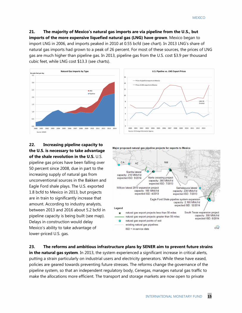
21. The majority of Mexico’s natural gas imports are via pipeline from the U.S., but
imports of the more expensive liquefied natural gas (LNG) have grown. Mexico began to
import LNG in 2006, and imports peaked in 2010 at 0.55 bcfd (see chart). In 2013 LNG’s share of
natural gas imports had grown to a peak of 26 percent. For most of these sources, the prices of LNG
gas are much higher than pipeline gas. In 2013, pipeline gas from the U.S. cost $3.9 per thousand
cubic feet, while LNG cost $13.3 (see charts).
22. Increasing pipeline capacity to
the U.S. is necessary to take advantage
of the shale revolution in the U.S. U.S.
pipeline gas prices have been falling over
50 percent since 2008, due in part to the
increasing supply of natural gas from
unconventional sources in the Bakken and
Eagle Ford shale plays. The U.S. exported
1.8 bcfd to Mexico in 2013, but projects
are in train to significantly increase that
amount. According to industry analysts,
between 2013 and 2016 about 5.2 bcfd in
pipeline capacity is being built (see map).
Delays in construction would delay
Mexico’s ability to take advantage of
lower-priced U.S. gas.
23. The reforms and ambitious infrastructure plans by SENER aim to prevent future strains
in the natural gas system. In 2013, the system experienced a significant increase in critical alerts,
putting a strain particularly on industrial users and electricity generators. While these have eased,
policies are geared towards preventing future stresses. The reforms change the governance of the
pipeline system, so that an independent regulatory body, Cenegas, manages natural gas traffic to
make the allocations more efficient. The transport and storage markets are now open to private
0.0
0.5
1.0
1.5
2.0
2.5
3.0
3.5
2000 2001 2002 2003 2004 2005 2006 2007 2008 2009 2010 2011 2012 2013 2014
Bn cubic feet per dayNatural Gas Imports by Type
LNG
Pipeline
Source: SENER
0
2
4
6
8
10
12
14
16
2000 2001 2002 2003 2004 2005 2006 2007 2008 2009 2010 2011 2012 2013
U.S. Pipeline vs. LNG Export Prices
Price of pipeline exports to Mexico
Price of LNG exports to Mexico
LNG 3XGreater
Source: US Energy Information Agency
MEXICO
16 INTERNATIONAL MONETARY FUND
participants, which will hopefully increase supply. Additionally, SENER has plans to build out the
domestic pipeline infrastructure to connect to the pipelines to the U.S. and expand the transport of
gas within Mexico.
I. Electricity Reform
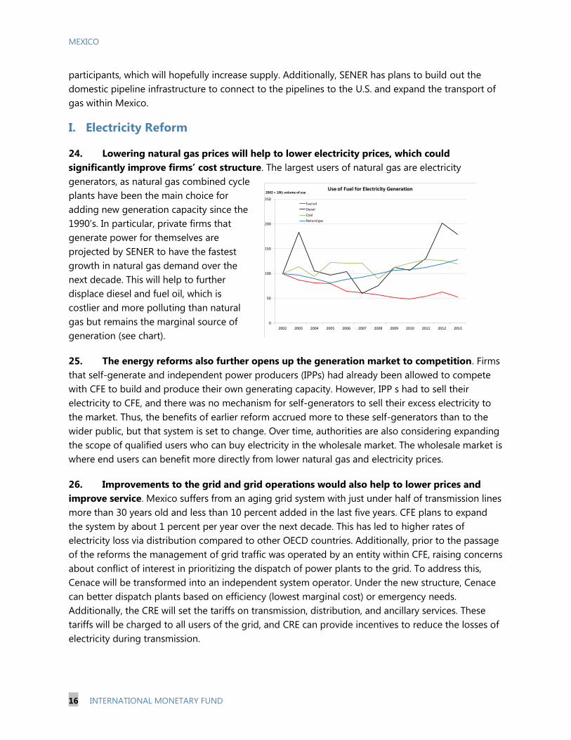
24. Lowering natural gas prices will help to lower electricity prices, which could
significantly improve firms’ cost structure. The largest users of natural gas are electricity
generators, as natural gas combined cycle
plants have been the main choice for
adding new generation capacity since the
1990’s. In particular, private firms that
generate power for themselves are
projected by SENER to have the fastest
growth in natural gas demand over the
next decade. This will help to further
displace diesel and fuel oil, which is
costlier and more polluting than natural
gas but remains the marginal source of
generation (see chart).
25. The energy reforms also further opens up the generation market to competition. Firms
that self-generate and independent power producers (IPPs) had already been allowed to compete
with CFE to build and produce their own generating capacity. However, IPP s had to sell their
electricity to CFE, and there was no mechanism for self-generators to sell their excess electricity to
the market. Thus, the benefits of earlier reform accrued more to these self-generators than to the
wider public, but that system is set to change. Over time, authorities are also considering expanding
the scope of qualified users who can buy electricity in the wholesale market. The wholesale market is
where end users can benefit more directly from lower natural gas and electricity prices.
26. Improvements to the grid and grid operations would also help to lower prices and
improve service. Mexico suffers from an aging grid system with just under half of transmission lines
more than 30 years old and less than 10 percent added in the last five years. CFE plans to expand
the system by about 1 percent per year over the next decade. This has led to higher rates of
electricity loss via distribution compared to other OECD countries. Additionally, prior to the passage
of the reforms the management of grid traffic was operated by an entity within CFE, raising concerns
about conflict of interest in prioritizing the dispatch of power plants to the grid. To address this,
Cenace will be transformed into an independent system operator. Under the new structure, Cenace
can better dispatch plants based on efficiency (lowest marginal cost) or emergency needs.
Additionally, the CRE will set the tariffs on transmission, distribution, and ancillary services. These
tariffs will be charged to all users of the grid, and CRE can provide incentives to reduce the losses of
electricity during transmission.
0
50
100
150
200
250
2002 2003 2004 2005 2006 2007 2008 2009 2010 2011 2012 2013
2002 = 100; volume of useUse of Fuel for Electricity Generation
Fuel oil
Diesel
Coal
Natural gas
MEXICO
INTERNATIONAL MONETARY FUND 17
27. The conversion of CFE into a state productive enterprise will give it more operational
and budgetary autonomy. It will also have an expanded ability to contract with third parties that
potentially could be more efficient at providing transmission and distribution services. CFE is also
charged with adopting international standards for the management of state enterprises aimed at
making its operations more efficient and lowering costs. This increased independence, as in the case
of Pemex, will hopefully lead to an improved ability to investment in energy infrastructure.
J. Conclusion
28. The energy reform is comprehensive and has the potential to reshape Mexico’s
economy to support faster growth, better living standards, and greater energy security. In the
short-run, it is a defensive reform aimed at overcoming the risk of falling hydrocarbons production
and improving the outlook for fiscal revenues. In the medium- to long-run, the reforms allow the
country to tap its potential in shale and deepwater, as well as to provide the incentives to reduce
domestic energy costs and improve services.
29. While the focus of market attention is on deepwater and shale, in the short-run
improvements in recovery and development of existing fields is crucial. Authorities have wisely
focused the majority of Round 1 on auctioning 2P fields that could yield hydrocarbons quickly.
Additionally, Pemex will now have more freedom to partner with third parties to increase investment
and import technologies to enhance its production.
30. The legislative hurdles have been tackled, but implementation risks remain. Round 1 is
critical and will set the tone for future rounds, and many changes to regulations and institutions still
have to be made. Delays or problems with implementation that dampen investor confidence will
have consequences. Our downside scenarios show a stylized illustration of the lower production
path and commensurate lower investments needs and FDI. These could have knock on negative
impacts on exports and fiscal revenues.
31. Managing expectations about the shale and deep water potential is critical. Patience is
needed given that it will take a long time before meaningful production can be extracted from these
sources.
32. While there has been so much focus on exploration and production, the pipes and the
grid are very important for growth. Lower energy costs and improving services will reap benefits
on the manufacturing sector and the broader economy. Planned natural gas pipeline projects will
help Mexico further lower its dependence on LNG, diesel, and fuel oil. Independent system
operators for natural gas and electricity will help to reduce critical alerts and enhance service
delivery.
33. Besides opening up the energy markets, Pemex and CFE needed to be shaken up to
improve their efficiency, costs, and ability to invest in infrastructure. Transforming them into
productive state enterprises and reducing their fiscal burdens are the first steps in this path.
MEXICO
18 INTERNATIONAL MONETARY FUND
References
Luna, Sergio, and Manriquez, Jorge Luis. Energy Reform and Investment Flows: How Much? When?.
Citi Economics Research, March 7, 2014.
Mattar, F., Murti, A. et al. Mexican Energy Reform. Goldman Sachs Equity Research, January 6, 2014.
Mexican Senate. Opinions of the Constitutional Commission on the Energy Sector.
Morse, Ed. Mind the Gulf: What does the North American energy revolution mean for Latin America?
Presentation at the Inter-American Dialogue, April 2014.
PEMEX. Mexico’s Energy Reform & PEMEX as a State Productive Enterprise. August, 2014
presentation.
PEMEX. Investor Presentation. May, 2014.
Press releases of Round 0 and 1 results (SENER website)
Secondary laws on the Mexican Energy Reform (SENER website).
Secretary of Energy, Mexico. Prospects of the Electricity Sector, 2013–2027.
Secretary of Energy, Mexico. Prospects of the Natural Gas and L.P. Gas, 2013–2027
U.S. Energy Information Agency. Mexico Country Briefing. April 24, 2014.
U.S. Energy Information Agency. Mexico Week. May 16, 2013.
U.S. Energy Information Agency. U.S. Natural Gas Exports to Mexico Reach a Record High in 2012.
March 13, 2013.
MEXICO
INTERNATIONAL MONETARY FUND 19
MADE IN MEXICO: THE ENERGY REFORM AND
MANUFACTURING OUTPUT1
A. Introduction
1. Manufacturing activity in Mexico surged after the signing of the North America Free
Trade Agreement, NAFTA. Since then, Mexico has attracted or created world-class performers in
the manufacturing sector. Greater integration and lower trade barriers with its largest trading
partner brought about new investment, new technology, and thus higher output. Today,
manufacturing exports account for about 80 percent of total exports, of which about a third
corresponds to automobiles.
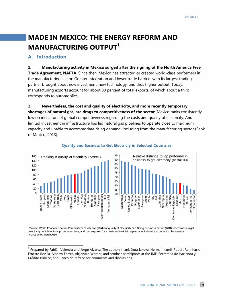
2. Nevertheless, the cost and quality of electricity, and more recently temporary
shortages of natural gas, are drags to competitiveness of the sector. Mexico ranks consistently
low on indicators of global competitiveness regarding the costs and quality of electricity. And
limited investment in infrastructure has led natural gas pipelines to operate close to maximum
capacity and unable to accommodate rising demand, including from the manufacturing sector (Bank
of Mexico, 2013).
Quality and Easiness to Get Electriciy in Selected Countries
1 Prepared by Fabián Valencia and Jorge Alvarez. The authors thank Dora Iakova, Herman Kamil, Robert Rennhack,
Ernesto Revilla, Alberto Torres, Alejandro Werner, and seminar participants at the IMF, Secretaría de Hacienda y
Crédito Público, and Banco de México for comments and discussions.
Source: World Economic Forum Competitiveness Report (2014) for quality of electricity and Doing Business Report (2014) for easiness to get electricity, which looks at procedures, time, and cost required for a business to obtain a permanent electricity connection for a newly constructed warehouse.
0
20
40
60
80
100
120
140
160
Un
ite
d S
tate
s
Uru
gu
ay
Co
sta
Ric
a
Pa
na
ma
Gu
ate
ma
la
Co
lom
bia
Ch
ile
Pe
ru
Bra
zil
El S
alv
ad
or
Me
xic
o
Ecu
ad
or
Ja
ma
ica
Nic
ara
gu
a
Bo
livia
Ho
nd
ura
s
Arg
en
tin
a
Pa
rag
ua
y
Do
min
ica
n R
ep
ub
lic
Ha
iti
Ve
ne
zu
ela
, RB
Ranking in quality of electricity (best=1)
50
55
60
65
70
75
80
85
90
95
Gu
ate
ma
la
Bra
zil
Un
ite
d S
tate
s
Pa
na
ma
Uru
gu
ay
Co
sta
Ric
a
Pa
rag
ua
y
Be
lize
Ch
ile
Pe
ru
Ha
iti
Co
lom
bia
Nic
ara
gu
a
Arg
en
tin
a
Ja
ma
ica
Do
min
ica
n R
ep
ub
lic
Ecu
ad
or
Me
xic
o
Ho
nd
ura
s
Bo
livia
Ve
ne
zu
ela
, RB
El S
alv
ad
or
Relative distance to top performer in easiness to get electricity (best=100)
MEXICO
20 INTERNATIONAL MONETARY FUND
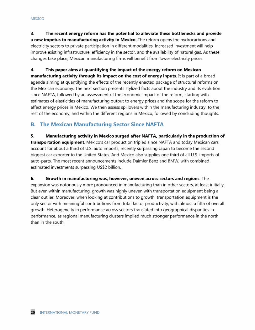
3. The recent energy reform has the potential to alleviate these bottlenecks and provide
a new impetus to manufacturing activity in Mexico. The reform opens the hydrocarbons and
electricity sectors to private participation in different modalities. Increased investment will help
improve existing infrastructure, efficiency in the sector, and the availability of natural gas. As these
changes take place, Mexican manufacturing firms will benefit from lower electricity prices.
4. This paper aims at quantifying the impact of the energy reform on Mexican
manufacturing activity through its impact on the cost of energy inputs. It is part of a broad
agenda aiming at quantifying the effects of the recently enacted package of structural reforms on
the Mexican economy. The next section presents stylized facts about the industry and its evolution
since NAFTA, followed by an assessment of the economic impact of the reform, starting with
estimates of elasticities of manufacturing output to energy prices and the scope for the reform to
affect energy prices in Mexico. We then assess spillovers within the manufacturing industry, to the
rest of the economy, and within the different regions in Mexico, followed by concluding thoughts.
B. The Mexican Manufacturing Sector Since NAFTA
5. Manufacturing activity in Mexico surged after NAFTA, particularly in the production of
transportation equipment. Mexico’s car production tripled since NAFTA and today Mexican cars
account for about a third of U.S. auto imports, recently surpassing Japan to become the second
biggest car exporter to the United States. And Mexico also supplies one third of all U.S. imports of
auto-parts. The most recent announcements include Daimler Benz and BMW, with combined
estimated investments surpassing US$2 billion.
6. Growth in manufacturing was, however, uneven across sectors and regions. The
expansion was notoriously more pronounced in manufacturing than in other sectors, at least initially.
But even within manufacturing, growth was highly uneven with transportation equipment being a
clear outlier. Moreover, when looking at contributions to growth, transportation equipment is the
only sector with meaningful contributions from total factor productivity, with almost a fifth of overall
growth. Heterogeneity in performance across sectors translated into geographical disparities in
performance, as regional manufacturing clusters implied much stronger performance in the north
than in the south.
MEXICO
INTERNATIONAL MONETARY FUND 21
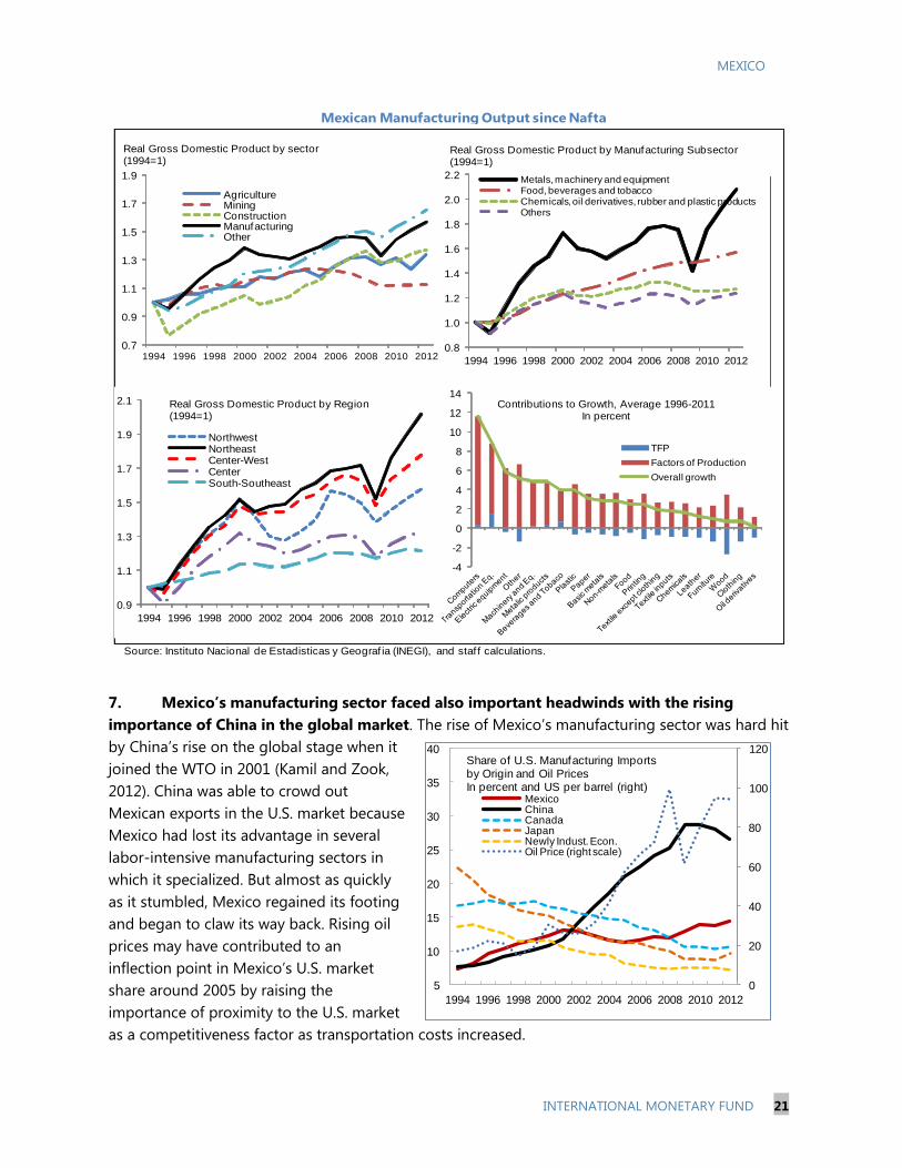
7. Mexico’s manufacturing sector faced also important headwinds with the rising
importance of China in the global market. The rise of Mexico’s manufacturing sector was hard hit
by China’s rise on the global stage when it
joined the WTO in 2001 (Kamil and Zook,
2012). China was able to crowd out
Mexican exports in the U.S. market because
Mexico had lost its advantage in several
labor-intensive manufacturing sectors in
which it specialized. But almost as quickly
as it stumbled, Mexico regained its footing
and began to claw its way back. Rising oil
prices may have contributed to an
inflection point in Mexico’s U.S. market
share around 2005 by raising the
importance of proximity to the U.S. market
as a competitiveness factor as transportation costs increased.
Mexican Manufacturing Output since Nafta
Source: Instituto Nacional de Estadisticas y Geograf ia (INEGI), and staf f calculations.
0.7
0.9
1.1
1.3
1.5
1.7
1.9
1994 1996 1998 2000 2002 2004 2006 2008 2010 2012
AgricultureMiningConstructionManufacturingOther
Real Gross Domestic Product by sector(1994=1)
0.8
1.0
1.2
1.4
1.6
1.8
2.0
2.2
1994 1996 1998 2000 2002 2004 2006 2008 2010 2012
Metals, machinery and equipmentFood, beverages and tobaccoChemicals, oil derivatives, rubber and plastic productsOthers
Real Gross Domestic Product by Manufacturing Subsector(1994=1)
0.9
1.1
1.3
1.5
1.7
1.9
2.1
1994 1996 1998 2000 2002 2004 2006 2008 2010 2012
NorthwestNortheastCenter-WestCenterSouth-Southeast
Real Gross Domestic Product by Region(1994=1)
-4
-2
0
2
4
6
8
10
12
14Contributions to Growth, Average 1996-2011
In percent
TFP
Factors of Production
Overall growth
0
20
40
60
80
100
120
5
10
15
20
25
30
35
40
1994 1996 1998 2000 2002 2004 2006 2008 2010 2012
MexicoChinaCanadaJapanNewly Indust. Econ.Oil Price (right scale)
Share of U.S. Manufacturing Imports by Origin and Oil PricesIn percent and US per barrel (right)
MEXICO
22 INTERNATIONAL MONETARY FUND
C. The Energy Reform: How Much of a Boost for Mexican Manufacturing?
8. While the energy reform can affect manufacturing production through several
channels, we focus on its effect through lower energy costs. The reform can lead to higher
capital accumulation as new investment arrives. And with this new investment, technology transfers
may also open the door to increases in overall productivity. However, at this juncture, there is
substantial uncertainty regarding these broader channels, but it is possible to infer how
manufacturing output would respond to lower energy prices from past data. Complemented with
estimates of the potential reduction in energy prices, these estimates can help us measure the
economic effects of the reform through its impact on energy prices and manufacturing activity.
How Sensitive is Manufacturing Output to Changes in Energy Prices?
9. We estimate the response of manufacturing output to changes in energy prices using
a simple panel regression analysis. The left-hand side corresponds to the real gross domestic
product for manufacturing industry i, in state j, in year t. The right hand-side includes a lag of the
dependent variable, the variables of interest: the lagged change in electricity prices, EL, in natural
gas prices, NG, and oil derivatives prices, OD. The focus on these particular energy inputs arises from
their importance in industrial production (Table 1). The change is computed after deflating energy
prices with the consumer’s price index to reflect changes in real terms. The regression includes
controls, X, in the equation below, that have been found to be important in explaining
manufacturing activity, including unit labor costs, the real effective exchange rate, the cost of capital,
industrial production in the United States, and other variables, all in first difference form. The
regressions include also fixed effects at the sector-state pair level, .
10. Among energy inputs, electricity prices have the largest impact on manufacturing
output, with an elasticity of up to -0.28. Tables 2 and 3 show the estimated elasticities under
various specifications for the most important energy sources. The elasticities range from -0.11 to -
0.28. For natural gas, the elasticities range from -0.04 to -0.07. The independent effect of natural gas,
aside from its impact through electricity prices, comes from the fact that about 18 percent of the
national demand for gas comes from the industrial sector, including manufacturing. The impact of a
one percent change in electricity prices far exceeds the one from natural gas prices. Interestingly, oil
derivatives come up with a positive sign. While in principle this positive coefficient could be picking
up the increased importance of proximity to U.S. as competitiveness factor in a world with rising oil
prices and transportation costs (Section I), it remains positive even after controlling for international
oil prices. Nevertheless, its statistical significance weakens as additional controls are included (Table
2, columns 5–7; Table 3, column 3)
MEXICO
INTERNATIONAL MONETARY FUND 23
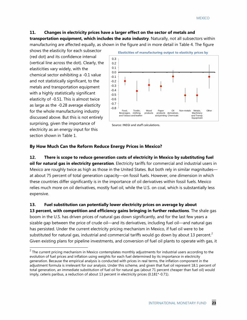
11. Changes in electricity prices have a larger effect on the sector of metals and
transportation equipment, which includes the auto industry. Naturally, not all subsectors within
manufacturing are affected equally, as shown in the figure and in more detail in Table 4. The figure
shows the elasticity for each subsector
(red dot) and its confidence interval
(vertical line across the dot). Clearly, the
elasticities vary widely, with the
chemical sector exhibiting a -0.1 value
and not statistically significant, to the
metals and transportation equipment
with a highly statistically significant
elasticity of -0.51. This is almost twice
as large as the -0.28 average elasticity
for the whole manufacturing industry
discussed above. But this is not entirely
surprising, given the importance of
electricity as an energy input for this
section shown in Table 1.
By How Much Can the Reform Reduce Energy Prices in Mexico?
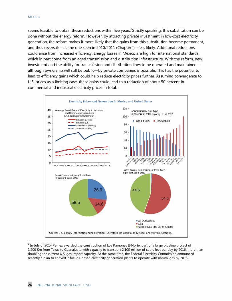
12. There is scope to reduce generation costs of electricity in Mexico by substituting fuel
oil for natural gas in electricity generation. Electricity tariffs for commercial and industrial users in
Mexico are roughly twice as high as those in the United States. But both rely in similar magnitudes—
at about 75 percent of total generation capacity—on fossil fuels. However, one dimension in which
these countries differ significantly is in the importance of oil derivatives within fossil fuels. Mexico
relies much more on oil derivatives, mostly fuel oil, while the U.S. on coal, which is substantially less
expensive.
13. Fuel substitution can potentially lower electricity prices on average by about
13 percent, with competition and efficiency gains bringing in further reductions. The shale gas
boom in the U.S. has driven prices of natural gas down significantly, and for the last few years a
sizable gap between the price of crude oil—and its derivatives, including fuel oil—and natural gas
has persisted. Under the current electricity pricing mechanism in Mexico, if fuel oil were to be
substituted for natural gas, industrial and commercial tariffs would go down by about 13 percent.2
Given existing plans for pipeline investments, and conversion of fuel oil plants to operate with gas, it
2 The current pricing mechanism in Mexico contemplates monthly adjustments for industrial users according to the
evolution of fuel prices and inflation using weights for each fuel determined by its importance in electricity
generation. Because the empirical analysis is conducted with prices in real terms, the inflation component in the
adjustment formula is irrelevant for our analysis. Under this scheme, and given that fuel oil represent 18.1 percent of
total generation, an immediate substitution of fuel oil for natural gas (about 71 percent cheaper than fuel oil) would
imply, ceteris paribus, a reduction of about 13 percent in electricity prices (0.181*-0.71).
-0.8
-0.7
-0.6
-0.5
-0.4
-0.3
-0.2
-0.1
0.0
0.1
0.2
0.3
Food, Beverages, and Tobaco
Textile, clothing,
and leather
Wood products
Paper products
and printing
Oil derivatives, Chemicals
Non-metals Metals, Machinery and Transp. Equipment
Other
Elasticities of manufacturing output to elasticity prices by
Source: INEGI and staff calculations.
MEXICO
24 INTERNATIONAL MONETARY FUND
seems feasible to obtain these reductions within five years.3Strictly speaking, this substitution can be
done without the energy reform. However, by attracting private investment in low-cost electricity
generation, the reform makes it more likely that the gains from this substitution become permanent,
and thus reversals—as the one seen in 2010/2011 (Chapter I)—less likely. Additional reductions
could arise from increased efficiency. Energy losses in Mexico are high for international standards,
which in part come from an aged transmission and distribution infrastructure. With the reform, new
investment and the ability for transmission and distribution lines to be operated and maintained—
although ownership will still be public—by private companies is possible. This has the potential to
lead to efficiency gains which could help reduce electricity prices further. Assuming convergence to
U.S. prices as a limiting case, these gains could lead to a reduction of about 50 percent in
commercial and industrial electricity prices in total.
3 In July of 2014 Pemex awarded the construction of Los Ramones II-Norte, part of a large pipeline project of
1,200 Km from Texas to Guanajuato with capacity to transport 2,100 million of cubic feet per day by 2016, more than
doubling the current U.S. gas import capacity. At the same time, the Federal Electricity Commission announced
recently a plan to convert 7 fuel oil-based electricity generation plants to operate with natural gas by 2016.
26.9
14.658.5
Mexico, composition of fossil fuelsIn percent, as of 2012
54.6
44.6
United States, composition of fossil fuelsIn percent, as of 2012
Oil DerivativesCoalNatural Gas and Other Gases
Source: U.S. Energy Information Administration, Secretaria de Energia de Mexico, and staff calculations.
0
20
40
60
80
100
120
Fossil Fuels Renewables
Generation by fuel type In percent of total capacity, as of 2012
0
5
10
15
20
25
30
35
40
2004 2005 2006 2007 2008 2009 2010 2011 2012 2013
Average Retail Price of Electricity to Industrial and Commercial Customers
(US$ cents per kilowatt/hour)
Industrial (Mexico)
Industrial (US)
Commercial (Mexico)
Commercial (US)
Electricity Prices and Generation in Mexico and United States
MEXICO
INTERNATIONAL MONETARY FUND 25
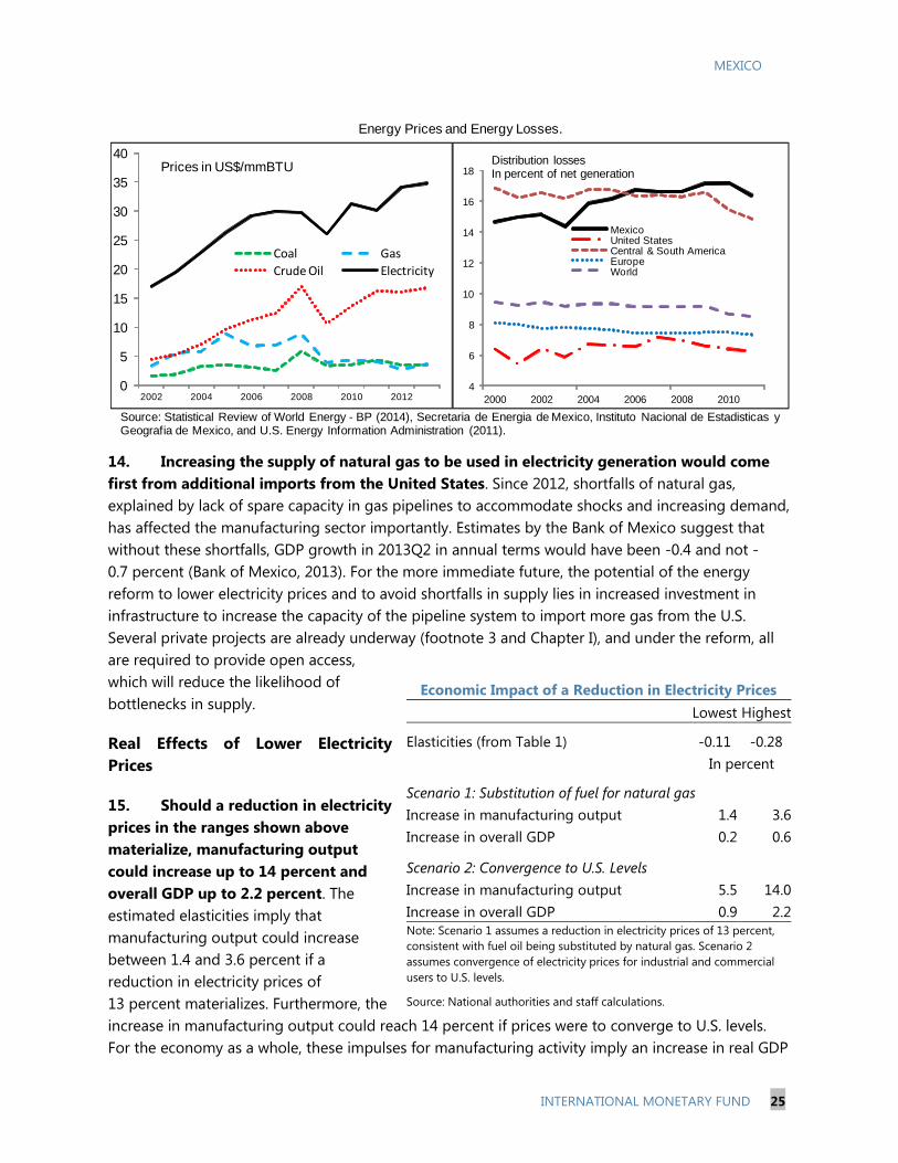
14. Increasing the supply of natural gas to be used in electricity generation would come
first from additional imports from the United States. Since 2012, shortfalls of natural gas,
explained by lack of spare capacity in gas pipelines to accommodate shocks and increasing demand,
has affected the manufacturing sector importantly. Estimates by the Bank of Mexico suggest that
without these shortfalls, GDP growth in 2013Q2 in annual terms would have been -0.4 and not -
0.7 percent (Bank of Mexico, 2013). For the more immediate future, the potential of the energy
reform to lower electricity prices and to avoid shortfalls in supply lies in increased investment in
infrastructure to increase the capacity of the pipeline system to import more gas from the U.S.
Several private projects are already underway (footnote 3 and Chapter I), and under the reform, all
are required to provide open access,
which will reduce the likelihood of
bottlenecks in supply.
Real Effects of Lower Electricity
Prices
15. Should a reduction in electricity
prices in the ranges shown above
materialize, manufacturing output
could increase up to 14 percent and
overall GDP up to 2.2 percent. The
estimated elasticities imply that
manufacturing output could increase
between 1.4 and 3.6 percent if a
reduction in electricity prices of
13 percent materializes. Furthermore, the
increase in manufacturing output could reach 14 percent if prices were to converge to U.S. levels.
For the economy as a whole, these impulses for manufacturing activity imply an increase in real GDP
4
6
8
10
12
14
16
18
2000 2002 2004 2006 2008 2010
MexicoUnited StatesCentral & South AmericaEuropeWorld
Distribution losses In percent of net generation
0
5
10
15
20
25
30
35
40
2002 2004 2006 2008 2010 2012
Coal Gas
Crude Oil Electricity
Prices in US$/mmBTU
Source: Statistical Review of World Energy - BP (2014), Secretaria de Energia de Mexico, Instituto Nacional de Estadisticas y Geografia de Mexico, and U.S. Energy Information Administration (2011).
Energy Prices and Energy Losses.
Economic Impact of a Reduction in Electricity Prices
Lowest Highest
Elasticities (from Table 1) -0.11
-0.28
In percent
Scenario 1: Substitution of fuel for natural gas
Increase in manufacturing output 1.4
3.6
Increase in overall GDP 0.2
0.6
Scenario 2: Convergence to U.S. Levels
Increase in manufacturing output 5.5
14.0
Increase in overall GDP 0.9 2.2
Note: Scenario 1 assumes a reduction in electricity prices of 13 percent,
consistent with fuel oil being substituted by natural gas. Scenario 2
assumes convergence of electricity prices for industrial and commercial
users to U.S. levels.
Source: National authorities and staff calculations.
MEXICO
26 INTERNATIONAL MONETARY FUND
of up to 0.6 percent and up to 2.2 percent for each scenario respectively, given today’s share of the
manufacturing sector in the economy. These level effects could materialize over the horizon that
takes electricity prices to exhibit these reductions. As mentioned before, it is reasonable to expect
the estimated gains under scenario 1 to materialize over 2016–2019. Timing of convergence of
prices to U.S. levels is more uncertain because it requires reducing energy losses in transmission and
distribution which is more challenging. Nevertheless, the scenario offers a benchmark of how large
the effects over the long-run can be.
16. Increased supply of natural gas could allow substituting LPG and reduce imports of
LNG; however, the effect of the reform on other energy prices is unclear. The industrial sector
in Mexico consumes about 10 percent of total LPG demanded in the country, which if substituted for
natural gas, it could provide an additional impetus to growth in manufacturing. Table 2 shows an
elasticity of about -0.09 for LPG prices, but this number may be capturing demand effects as well,
and thus it should be interpreted with caution.4 And more broadly, increased availability of natural
gas imported through pipelines can reduce and possibly even eliminate, in the long run, the need to
import it in liquid form (LNG). Estimating the impact of the energy reform on oil and oil derivatives
prices is more complex because those are commodities which are influenced by global demand and
supply.
D. Are There Additional Indirect Effects Through Spillovers?
17. To allow for endogenous responses of unit labor costs and assess spillover effects we
turn to a panel vector autoregression framework (VAR).5 The results shown in the previous
section highlight the direct impact of changes in energy prices on manufacturing output. However,
there may be indirect effects that could imply lower or higher total effects on manufacturing output
from changes in energy prices. For instance, unit labor costs may react to changes in energy prices,
analogously to how they react to oil-price shocks (Blanchard and Gali, 2007), because of a potential
substitution effect that induces an increase in labor demand or to labor supply channels associated
with higher costs of living if changes in energy prices are passed to prices of good and services.
Similarly, a subsector within manufacturing may respond directly to energy prices and indirectly
through its dependence on other subsectors. Using the same logic, we explore regional spillovers.
We focus our attention on electricity prices which as shown before are the ones with the largest
impact on output.
4 LPG represents less than 3 percent of energy inputs in the industrial sector and for this reason the estimated
elasticity would seem high, suggesting that it may be capturing also the impact of LPG prices on manufacturing
through its effect on demand.
5 Appendix A provides technical details about the VAR specification. A more detailed technical discussion and several
robustness exercises are also provided in Alvarez and Valencia (forthcoming).
MEXICO
INTERNATIONAL MONETARY FUND 27
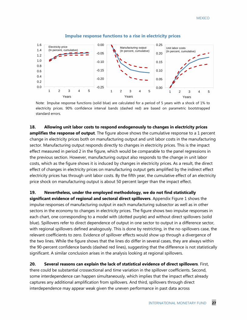
18. Allowing unit labor costs to respond endogenously to changes in electricity prices
amplifies the response of output. The figure above shows the cumulative response to a 1 percent
change in electricity prices both on manufacturing output and unit labor costs in the manufacturing
sector. Manufacturing output responds directly to changes in electricity prices. This is the impact
effect measured in period 2 in the figure, which would be comparable to the panel regressions in
the previous section. However, manufacturing output also responds to the change in unit labor
costs, which as the figure shows it is induced by changes in electricity prices. As a result, the direct
effect of changes in electricity prices on manufacturing output gets amplified by the indirect effect
electricity prices has through unit labor costs. By the fifth year, the cumulative effect of an electricity
price shock on manufacturing output is about 50 percent larger than the impact effect.
19. Nevertheless, under the employed methodology, we do not find statistically
significant evidence of regional and sectoral direct spillovers. Appendix Figure 1 shows the
impulse responses of manufacturing output in each manufacturing subsector as well as in other
sectors in the economy to changes in electricity prices. The figure shows two impulse responses in
each chart, one corresponding to a model with (dotted purple) and without direct spillovers (solid
blue). Spillovers refer to direct dependence of output in one sector to output in a difference sector,
with regional spillovers defined analogously. This is done by restricting, in the no-spillovers case, the
relevant coefficients to zero. Evidence of spillover effects would show up through a divergence of
the two lines. While the figure shows that the lines do differ in several cases, they are always within
the 90-percent confidence bands (dashed red lines), suggesting that the difference is not statistically
significant. A similar conclusion arises in the analysis looking at regional spillovers.
20. Several reasons can explain the lack of statistical evidence of direct spillovers. First,
there could be substantial crossectional and time variation in the spillover coefficients. Second,
some interdependence can happen simultaneously, which implies that the impact effect already
captures any additional amplification from spillovers. And third, spillovers through direct
interdependence may appear weak given the uneven performance in past data across
Impulse response functions to a rise in electricity prices
Note: Impulse response functions (solid blue) are calculated for a period of 5 years with a shock of 1% to
electricity prices. 90% confidence interval bands (dashed red) are based on parametric bootstrapped
standard errors.
0.0
0.2
0.4
0.6
0.8
1.0
1.2
1.4
1.6
1 2 3 4 5
Years
Electricity price(In percent, cumulative)
-0.25
-0.20
-0.15
-0.10
-0.05
0.00
1 2 3 4 5
Years
Manufacturing output(In percent, cumulative)
0.00
0.05
0.10
0.15
0.20
0.25
1 2 3 4 5
Years
Unit labor costs(In percent, cumulative)
MEXICO
28 INTERNATIONAL MONETARY FUND
manufacturing subsectors and regions. In sum, direct spillovers of the kind explored in this paper
and under the chosen methodology do not appear statistically strong. These results are however not
conclusive given the caveats noted above.
E. Concluding Remarks and Policy Implications
21. The energy reform is likely to have important real effects through its impact on
manufacturing activity through lower electricity prices. These effects would come on top of the
direct effects on growth that would arise from increased investment and production in the energy
sector, for instance, from oil and gas exploration and extraction. Other factors, such as technology
spillovers and increased foreign direct investment in manufacturing as the sector becomes more
competitive could amplify the effects estimated in this paper.
22. In terms of policy priorities, increasing gas pipeline capacity to allow larger natural gas
imports from the U.S. will yield the most immediate gains. In addition, existing fuel oil-based
plants would need to be adapted to operate with natural gas. This would allow collecting the low-
hanging fruit associated with substitution of fuel oil for natural gas in electricity generation. As the
reform starts attracting private investment in low-cost electricity generation, the gains from fuel
substitution are more likely to become permanent. Further gains will follow from increasing
availability of gas throughout the country by an expanded network of pipelines.
23. A strong regulator is critical to ensuring competition in electricity generation and thus
making any reduction in electricity prices long-lasting. To this end, synergy with the antitrust
reform will play an important role. The new antitrust framework should help ensure an efficient
opening of the sector to private investment to ensure healthy competition.
24. For gains in efficiency, it is critical that the operation of transmission and distribution
lines encompass the right incentives to improve existing infrastructure. As distribution and
transmission lines will remain property of the state, gains in efficiency will arise from having in place
the right incentives for the new administrator of the infrastructure to invest and lower the high
technical losses in the system. A word of caution is needed. Reducing distribution losses will be
challenging and thus the gains from increased efficiency, while in theory are important, are not
guaranteed.
MEXICO
INTERNATIONAL MONETARY FUND 29
References
Alvarez and Valencia, forthcoming. “Made in Mexico: Energy Reform and Manufacturing Growth.”
IMF Working paper.
Bank of Mexico, 2013. “Efectos del Desabasto de Gas Natural sobre la Actividad Económica.”
Informe sobre la Inflación, Julio–Septiembre 2013, pp. 31–34.
Blanchard, O. J., & Gali, J. (2007). The Macroeconomic Effects of Oil Shocks: Why are the 2000s so
different from the 1970s? (No. w13368). National Bureau of Economic Research.
Kamil, H & Zook, J., 2012. “What Explains Mexico’s Recovery of U.S. Market Share?” IMF Article IV
Consultation. Selected Issues, 16–25.
MEXICO
30 INTERNATIONAL MONETARY FUND
Table 1. Energy Consumption (in Petajoules) of the Industrial Sector
2010 2011 2012
Industrial sector total 1,381.1 1,492.3 1,530.6
Electricity 34.2% 33.6% 34.5%
Natural Gas 35.3% 35.2% 35.8%
Oil derivatives 17.0% 15.5% 15.6%
Others 13.5% 15.8% 14.0%
Auto industry 10.5 12.7 14.4
Electricity 68.3% 60.0% 60.4%
Natural Gas 19.9% 28.1% 28.7%
Oil derivatives 11.8% 11.9% 10.9%
Others 0.0% 0.0% 0.0%
Source: SENER. Balance Nacional de Energía.
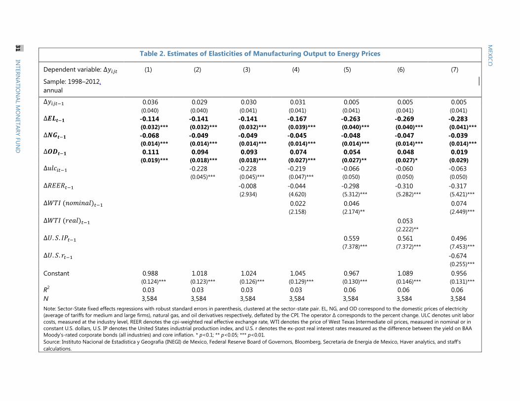
Table 2. Estimates of Elasticities of Manufacturing Output to Energy Prices
Dependent variable:
Sample: 1998–2012,
annual
(1) (2) (3) (4) (5) (6) (7)
0.036 0.029 0.030 0.031 0.005 0.005 0.005 (0.040) (0.040) (0.041) (0.041) (0.041) (0.041) (0.041)
-0.114 -0.141 -0.141 -0.167 -0.263 -0.269 -0.283 (0.032)*** (0.032)*** (0.032)*** (0.039)*** (0.040)*** (0.040)*** (0.041)***
-0.068 -0.049 -0.049 -0.045 -0.048 -0.047 -0.039 (0.014)*** (0.014)*** (0.014)*** (0.014)*** (0.014)*** (0.014)*** (0.014)***
0.111 0.094 0.093 0.074 0.054 0.048 0.019 (0.019)*** (0.018)*** (0.018)*** (0.027)*** (0.027)** (0.027)* (0.029)
-0.228 -0.228 -0.219 -0.066 -0.060 -0.063 (0.045)*** (0.045)*** (0.047)*** (0.050) (0.050) (0.050)
-0.008 -0.044 -0.298 -0.310 -0.317 (2.934) (4.620) (5.312)*** (5.282)*** (5.421)***
0.022 0.046 0.074 (2.158) (2.174)** (2.449)***
0.053
(2.222)**
0.559 0.561 0.496 (7.378)*** (7.372)*** (7.453)***
-0.674 (0.255)***
Constant 0.988 1.018 1.024 1.045 0.967 1.089 0.956 (0.124)*** (0.123)*** (0.126)*** (0.129)*** (0.130)*** (0.146)*** (0.131)***
R2 0.03 0.03 0.03 0.03 0.06 0.06 0.06
N 3,584 3,584 3,584 3,584 3,584 3,584 3,584
Note: Sector-State fixed effects regressions with robust standard errors in parenthesis, clustered at the sector-state pair. EL, NG, and OD correspond to the domestic prices of electricity
(average of tariffs for medium and large firms), natural gas, and oil derivatives respectively, deflated by the CPI. The operator ∆ corresponds to the percent change. ULC denotes unit labor
costs, measured at the industry level, REER denotes the cpi-weighted real effective exchange rate, WTI denotes the price of West Texas Intermediate oil prices, measured in nominal or in
constant U.S. dollars, U.S. IP denotes the United States industrial production index, and U.S. r denotes the ex-post real interest rates measured as the difference between the yield on BAA
Moody’s-rated corporate bonds (all industries) and core inflation. * p<0.1; ** p<0.05; *** p<0.01.
Source: Instituto Nacional de Estadística y Geografia (INEGI) de Mexico, Federal Reserve Board of Governors, Bloomberg, Secretaria de Energia de Mexico, Haver analytics, and staff’s
calculations.
MEX
ICO
31
IN
TER
NA
TIO
NA
L MO
NETA
RY F
UN
D
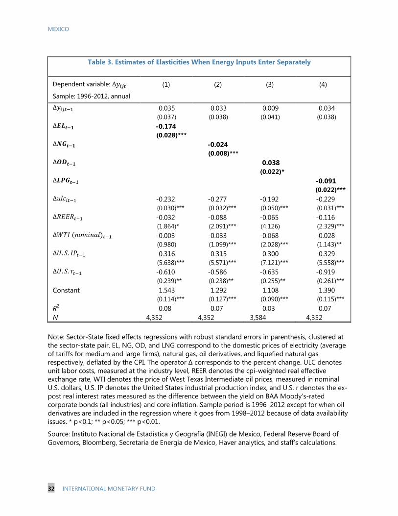
MEXICO
32 INTERNATIONAL MONETARY FUND
Table 3. Estimates of Elasticities When Energy Inputs Enter Separately
Dependent variable:
Sample: 1996-2012, annual
(1) (2) (3) (4)
0.035 0.033 0.009 0.034
(0.037) (0.038) (0.041) (0.038)
-0.174
(0.028)***
-0.024
(0.008)***
0.038
(0.022)*
-0.091
(0.022)***
-0.232 -0.277 -0.192 -0.229
(0.030)*** (0.032)*** (0.050)*** (0.031)***
-0.032 -0.088 -0.065 -0.116
(1.864)* (2.091)*** (4.126) (2.329)***
-0.003 -0.033 -0.068 -0.028
(0.980) (1.099)*** (2.028)*** (1.143)**
0.316 0.315 0.300 0.329
(5.638)*** (5.571)*** (7.121)*** (5.558)***
-0.610 -0.586 -0.635 -0.919
(0.239)** (0.238)** (0.255)** (0.261)***
Constant 1.543 1.292 1.108 1.390
(0.114)*** (0.127)*** (0.090)*** (0.115)***
R2 0.08 0.07 0.03 0.07
N 4,352 4,352 3,584 4,352
Note: Sector-State fixed effects regressions with robust standard errors in parenthesis, clustered at
the sector-state pair. EL, NG, OD, and LNG correspond to the domestic prices of electricity (average
of tariffs for medium and large firms), natural gas, oil derivatives, and liquefied natural gas
respectively, deflated by the CPI. The operator ∆ corresponds to the percent change. ULC denotes
unit labor costs, measured at the industry level, REER denotes the cpi-weighted real effective
exchange rate, WTI denotes the price of West Texas Intermediate oil prices, measured in nominal
U.S. dollars, U.S. IP denotes the United States industrial production index, and U.S. r denotes the ex-
post real interest rates measured as the difference between the yield on BAA Moody’s-rated
corporate bonds (all industries) and core inflation. Sample period is 1996–2012 except for when oil
derivatives are included in the regression where it goes from 1998–2012 because of data availability
issues. * p<0.1; ** p<0.05; *** p<0.01.
Source: Instituto Nacional de Estadística y Geografia (INEGI) de Mexico, Federal Reserve Board of
Governors, Bloomberg, Secretaria de Energia de Mexico, Haver analytics, and staff’s calculations.
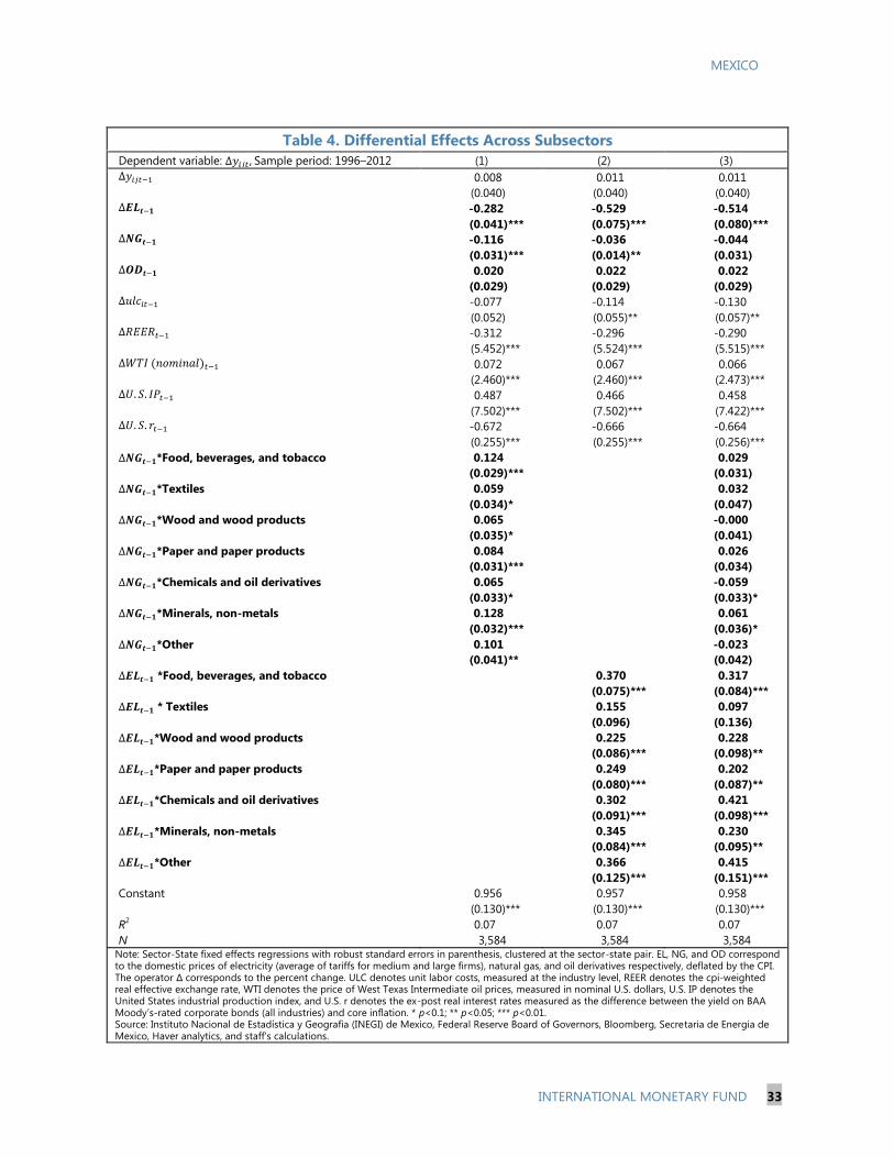
MEXICO
INTERNATIONAL MONETARY FUND 33
Table 4. Differential Effects Across Subsectors
Dependent variable: Sample period: 1996–2012 (1) (2) (3)
0.008 0.011 0.011
(0.040) (0.040) (0.040)
-0.282 -0.529 -0.514
(0.041)*** (0.075)*** (0.080)***
-0.116 -0.036 -0.044
(0.031)*** (0.014)** (0.031)
0.020 0.022 0.022
(0.029) (0.029) (0.029)
-0.077 -0.114 -0.130
(0.052) (0.055)** (0.057)**
-0.312 -0.296 -0.290
(5.452)*** (5.524)*** (5.515)***
0.072 0.067 0.066
(2.460)*** (2.460)*** (2.473)***
0.487 0.466 0.458
(7.502)*** (7.502)*** (7.422)***
-0.672 -0.666 -0.664
(0.255)*** (0.255)*** (0.256)***
*Food, beverages, and tobacco 0.124 0.029
(0.029)*** (0.031)
*Textiles 0.059 0.032
(0.034)* (0.047)
*Wood and wood products 0.065 -0.000
(0.035)* (0.041)
*Paper and paper products 0.084 0.026
(0.031)*** (0.034)
*Chemicals and oil derivatives 0.065 -0.059
(0.033)* (0.033)*
*Minerals, non-metals 0.128 0.061
(0.032)*** (0.036)*
*Other 0.101 -0.023
(0.041)** (0.042)
*Food, beverages, and tobacco 0.370 0.317
(0.075)*** (0.084)***
* Textiles 0.155 0.097
(0.096) (0.136)
*Wood and wood products 0.225 0.228
(0.086)*** (0.098)**
*Paper and paper products 0.249 0.202
(0.080)*** (0.087)**
*Chemicals and oil derivatives 0.302 0.421
(0.091)*** (0.098)***
*Minerals, non-metals 0.345 0.230
(0.084)*** (0.095)**
*Other 0.366 0.415
(0.125)*** (0.151)***
Constant 0.956 0.957 0.958
(0.130)*** (0.130)*** (0.130)***
R2 0.07 0.07 0.07
N 3,584 3,584 3,584 Note: Sector-State fixed effects regressions with robust standard errors in parenthesis, clustered at the sector-state pair. EL, NG, and OD correspond to the domestic prices of electricity (average of tariffs for medium and large firms), natural gas, and oil derivatives respectively, deflated by the CPI. The operator ∆ corresponds to the percent change. ULC denotes unit labor costs, measured at the industry level, REER denotes the cpi-weighted real effective exchange rate, WTI denotes the price of West Texas Intermediate oil prices, measured in nominal U.S. dollars, U.S. IP denotes the United States industrial production index, and U.S. r denotes the ex-post real interest rates measured as the difference between the yield on BAA Moody’s-rated corporate bonds (all industries) and core inflation. * p<0.1; ** p<0.05; *** p<0.01. Source: Instituto Nacional de Estadística y Geografia (INEGI) de Mexico, Federal Reserve Board of Governors, Bloomberg, Secretaria de Energia de Mexico, Haver analytics, and staff’s calculations.
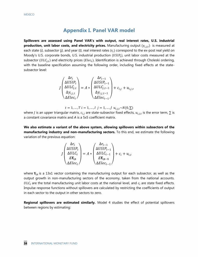
MEXICO
34 INTERNATIONAL MONETARY FUND
Appendix I. Panel VAR model
Spillovers are assessed using Panel VAR’s with output, real interest rates, U.S. industrial
production, unit labor costs, and electricity prices. Manufacturing output ( is measured at
each state (i), subsector (j), and year (t), real interest rates ( correspond to the ex-post real yield on
Moody’s U.S. corporate bonds, U.S. industrial production ( ), unit labor costs measured at the
subsector and electricity prices ( . Identification is achieved through Choleski ordering,
with the baseline specification assuming the following order, including fixed effects at the state-
subsector level:
where is an upper triangular matrix, are state-subsector fixed effects, is the error term, ∑ is
a constant covariance matrix and A is a 5x5 coefficient matrix.
We also estimate a variant of the above system, allowing spillovers within subsectors of the
manufacturing industry and non-manufacturing sectors. To this end, we estimate the following
variation of the previous equation:
where is a 13x1 vector containing the manufacturing output for each subsector, as well as the
output growth in non-manufacturing sectors of the economy, taken from the national accounts.
are the total manufacturing unit labor costs at the national level, and are state fixed effects.
Impulse response functions without spillovers are calculated by restricting the coefficients of output
in each sector to the output in other sectors to zero.
Regional spillovers are estimated similarly. Model 4 studies the effect of potential spillovers
between regions by estimating:
,
, ,
= 𝐴 ∗
−1
−1
, −1
, , −1
−1
+ , + , ,
,
= 𝐴 ∗
−1
−1
−1
, −
−1
+ + ,
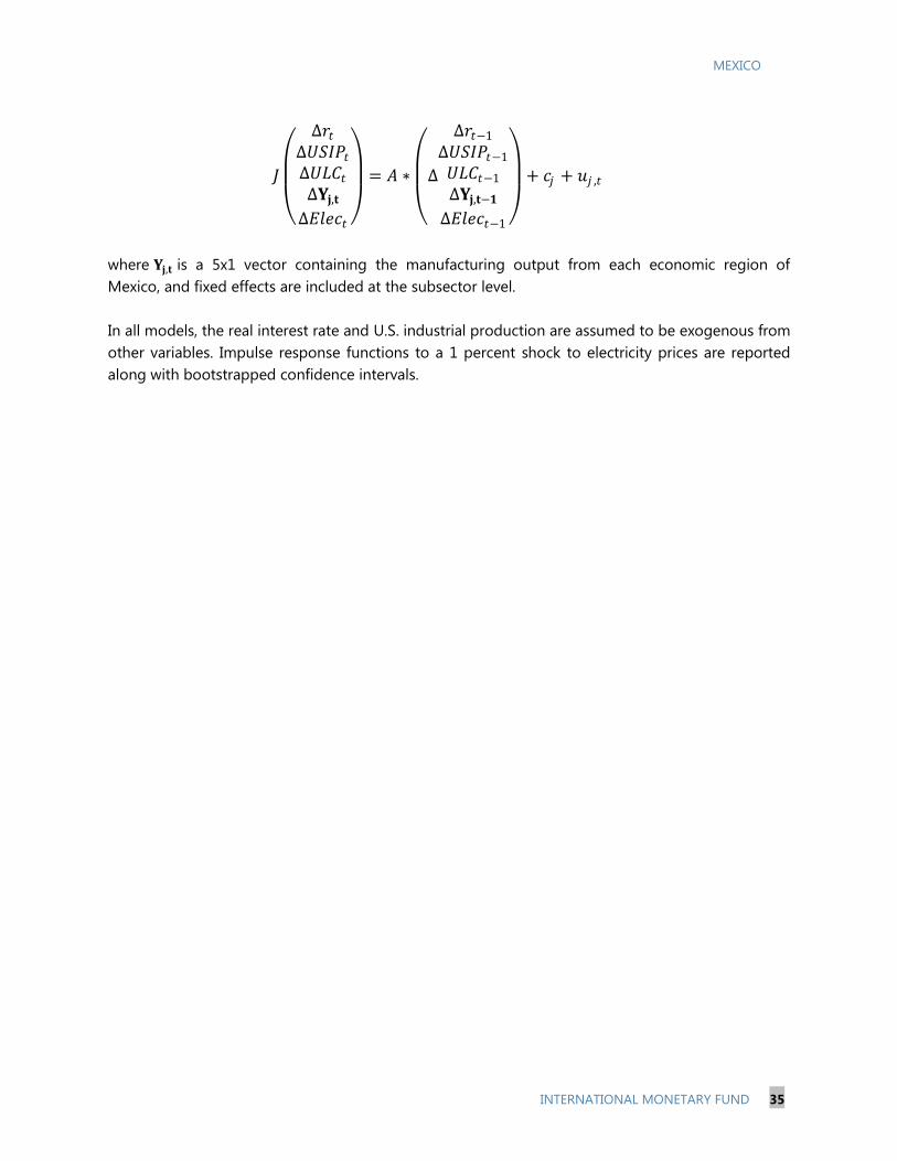
MEXICO
INTERNATIONAL MONETARY FUND 35
where is a 5x1 vector containing the manufacturing output from each economic region of
Mexico, and fixed effects are included at the subsector level.
In all models, the real interest rate and U.S. industrial production are assumed to be exogenous from
other variables. Impulse response functions to a 1 percent shock to electricity prices are reported
along with bootstrapped confidence intervals.
,
= 𝐴 ∗
−1
−1
−1
, −
−1
+ + ,
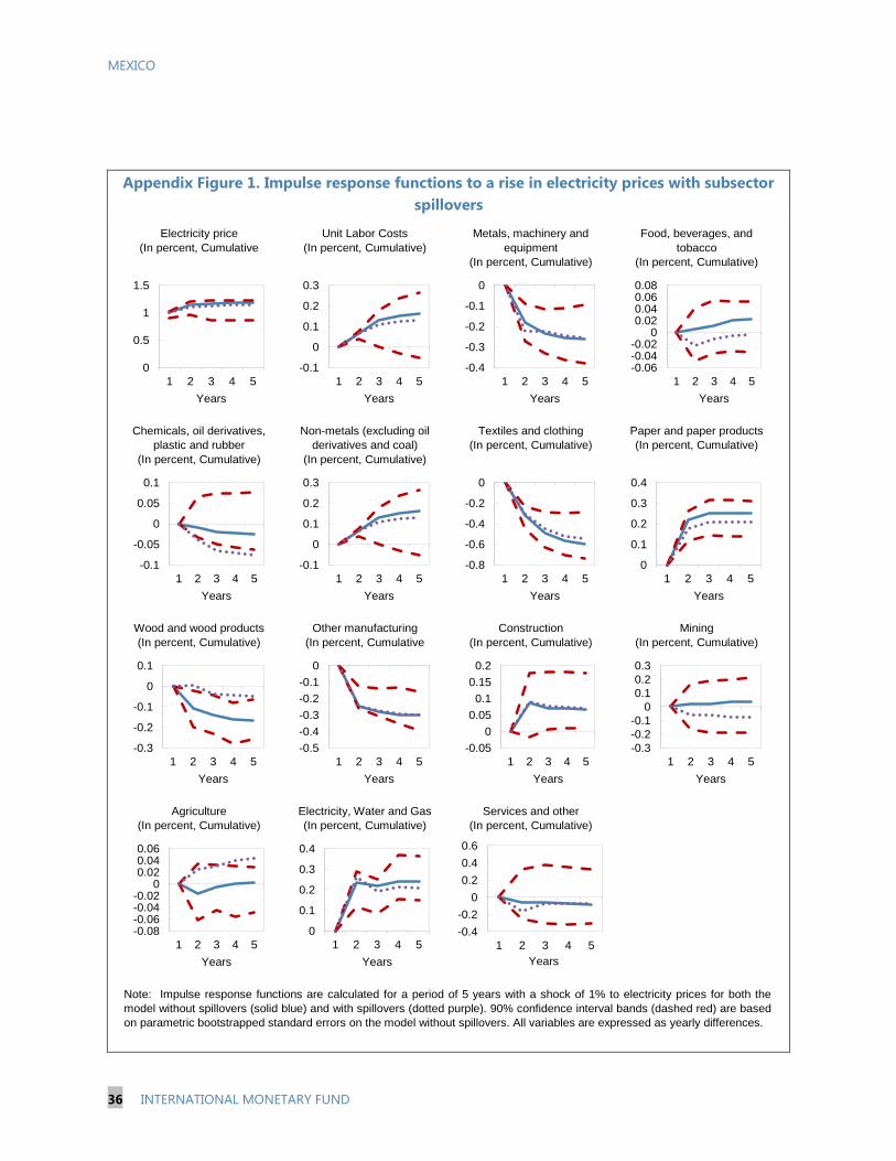
MEXICO
36 INTERNATIONAL MONETARY FUND
Appendix Figure 1. Impulse response functions to a rise in electricity prices with subsector
spillovers
Appendix Figure 1. Impulse response functions to a rise in electricity prices with
subsector spillovers
Electricity price
(In percent, Cumulative
Unit Labor Costs
(In percent, Cumulative)
Metals, machinery and
equipment
(In percent, Cumulative)
Food, beverages, and
tobacco
(In percent, Cumulative)
Chemicals, oil derivatives,
plastic and rubber
(In percent, Cumulative)
Non-metals (excluding oil
derivatives and coal)
(In percent, Cumulative)
Textiles and clothing
(In percent, Cumulative)
Paper and paper products
(In percent, Cumulative)
Wood and wood products
(In percent, Cumulative)
Other manufacturing
(In percent, Cumulative
Construction
(In percent, Cumulative)
Mining
(In percent, Cumulative)
Agriculture
(In percent, Cumulative)
Electricity, Water and Gas
(In percent, Cumulative)
Services and other
(In percent, Cumulative)
Note: Impulse response functions are calculated for a period of 5 years with a shock of 1% to electricity prices for both the
model without spillovers (solid blue) and with spillovers (dotted purple). 90% confidence interval bands (dashed red) are based
on parametric bootstrapped standard errors on the model without spillovers. All variables are expressed as yearly differences.
0
0.5
1
1.5
1 2 3 4 5
Years
-0.1
0
0.1
0.2
0.3
1 2 3 4 5
Years
-0.4
-0.3
-0.2
-0.1
0
1 2 3 4 5
Years
-0.06-0.04-0.02
00.020.040.060.08
1 2 3 4 5
Years
-0.1
-0.05
0
0.05
0.1
1 2 3 4 5
Years
-0.1
0
0.1
0.2
0.3
1 2 3 4 5
Years
-0.8
-0.6
-0.4
-0.2
0
1 2 3 4 5
Years
0
0.1
0.2
0.3
0.4
1 2 3 4 5
Years
-0.3
-0.2
-0.1
0
0.1
1 2 3 4 5
Years
-0.5
-0.4
-0.3
-0.2
-0.1
0
1 2 3 4 5
Years
-0.05
0
0.05
0.1
0.15
0.2
1 2 3 4 5
Years
-0.3
-0.2
-0.1
0
0.1
0.2
0.3
1 2 3 4 5
Years
-0.08-0.06-0.04-0.02
00.020.040.06
1 2 3 4 5
Years
0
0.1
0.2
0.3
0.4
1 2 3 4 5
Years
-0.4
-0.2
0
0.2
0.4
0.6
1 2 3 4 5
Years
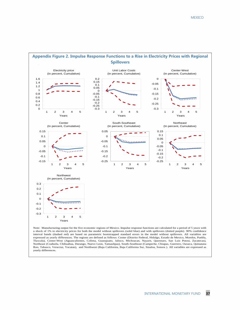
MEXICO
INTERNATIONAL MONETARY FUND 37
Appendix Figure 2. Impulse Response Functions to a Rise in Electricity Prices with Regional
Spillovers
Appendix Figure 2. Impulse response functions to a rise in electricity prices with
regional spillovers
Electricity price
(In percent, Cumulative)
Unit Labor Costs
(In percent, Cumulative)
Center-West
(In percent, Cumulative)
Center
(In percent, Cumulative)
South-Southeast
(In percent, Cumulative)
Northeast
(In percent, Cumulative)
Northwest
(In percent, Cumulative)
Note: Manufacturing output for the five economic regions of Mexico. Impulse response functions are calculated for a period of 5 years with
a shock of 1% to electricity prices for both the model without spillovers (solid blue) and with spillovers (dotted purple). 90% confidence
interval bands (dashed red) are based on parametric bootstrapped standard errors in the model without spillovers. All variables are
expressed as yearly differences. The regions are defined as follows: Center (Distrito Federal, Hidalgo, Estado de Mexico, Morelos, Puebla,
Tlaxcala), Center-West (Aguascalientes, Colima, Guanajuato, Jalisco, Michoacan, Nayarit, Queretaro, San Luis Potosi, Zacatecas),
Northeast (Coahuila, Chihuahua, Durango, Nuevo Leon, Tamaulipas), South-Southeast (Campeche, Chiapas, Guerrero, Oaxaca, Quinatana
Roo, Tabasco, Veracruz, Yucatan), and Northwest (Baja California, Baja California Sur, Sinaloa, Sonora ). All variables are expressed as
yearly differences.
0
0.2
0.4
0.6
0.8
1
1.2
1.4
1.6
1 2 3 4 5
Years
-0.3
-0.25
-0.2
-0.15
-0.1
-0.05
0
0.05
0.1
0.15
0.2
1 2 3 4 5
Years
-0.3
-0.25
-0.2
-0.15
-0.1
-0.05
0
1 2 3 4 5
Years
-0.15
-0.1
-0.05
0
0.05
0.1
0.15
1 2 3 4 5
Years
-0.25
-0.2
-0.15
-0.1
-0.05
0
0.05
1 2 3 4 5
Years
-0.25
-0.2
-0.15
-0.1
-0.05
0
0.05
0.1
0.15
1 2 3 4 5
Years
-0.3
-0.2
-0.1
0
0.1
0.2
0.3
1 2 3 4 5
Years
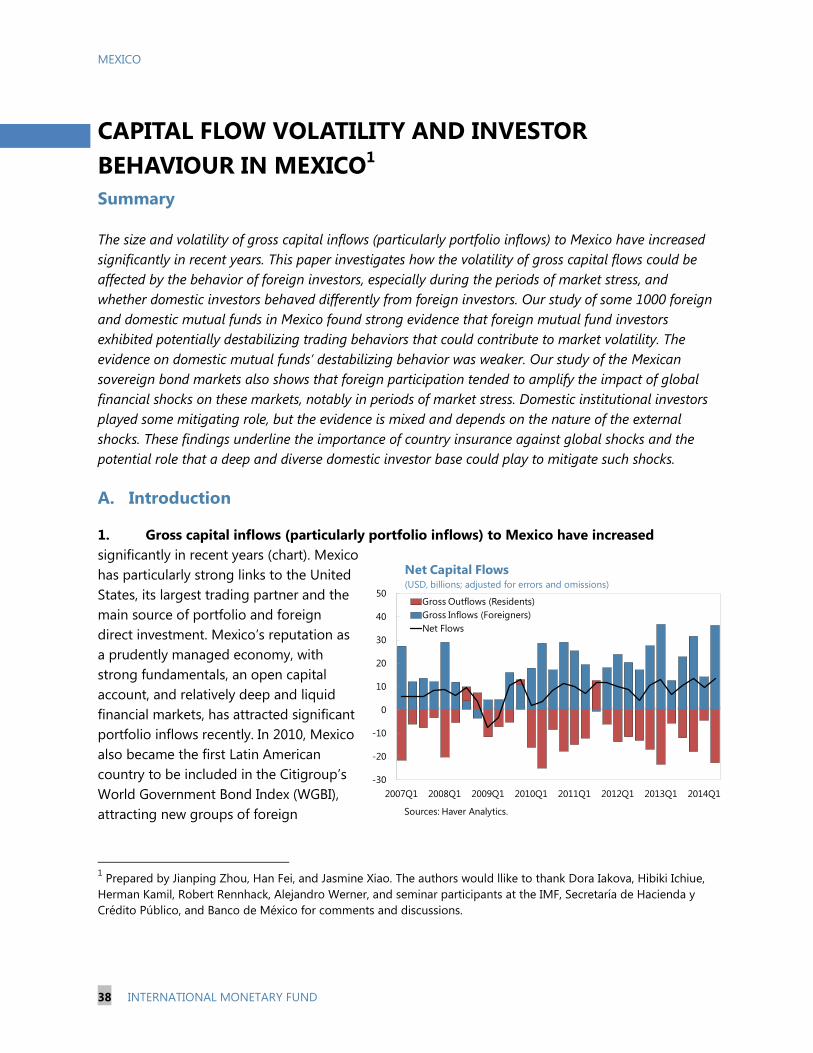
MEXICO
38 INTERNATIONAL MONETARY FUND
CAPITAL FLOW VOLATILITY AND INVESTOR
BEHAVIOUR IN MEXICO1
Summary The size and volatility of gross capital inflows (particularly portfolio inflows) to Mexico have increased
significantly in recent years. This paper investigates how the volatility of gross capital flows could be
affected by the behavior of foreign investors, especially during the periods of market stress, and
whether domestic investors behaved differently from foreign investors. Our study of some 1000 foreign
and domestic mutual funds in Mexico found strong evidence that foreign mutual fund investors
exhibited potentially destabilizing trading behaviors that could contribute to market volatility. The
evidence on domestic mutual funds’ destabilizing behavior was weaker. Our study of the Mexican
sovereign bond markets also shows that foreign participation tended to amplify the impact of global
financial shocks on these markets, notably in periods of market stress. Domestic institutional investors
played some mitigating role, but the evidence is mixed and depends on the nature of the external
shocks. These findings underline the importance of country insurance against global shocks and the
potential role that a deep and diverse domestic investor base could play to mitigate such shocks.
A. Introduction
1. Gross capital inflows (particularly portfolio inflows) to Mexico have increased
significantly in recent years (chart). Mexico
has particularly strong links to the United
States, its largest trading partner and the
main source of portfolio and foreign
direct investment. Mexico’s reputation as
a prudently managed economy, with
strong fundamentals, an open capital
account, and relatively deep and liquid
financial markets, has attracted significant
portfolio inflows recently. In 2010, Mexico
also became the first Latin American
country to be included in the Citigroup’s
World Government Bond Index (WGBI),
attracting new groups of foreign
1 Prepared by Jianping Zhou, Han Fei, and Jasmine Xiao. The authors would llike to thank Dora Iakova, Hibiki Ichiue,
Herman Kamil, Robert Rennhack, Alejandro Werner, and seminar participants at the IMF, Secretaría de Hacienda y
Crédito Público, and Banco de México for comments and discussions.
-30
-20
-10
0
10
20
30
40
50
2007Q1 2008Q1 2009Q1 2010Q1 2011Q1 2012Q1 2013Q1 2014Q1
Gross Outflows (Residents)
Gross Inflows (Foreigners)
Net Flows
Net Capital Flows(USD, billions; adjusted for errors and omissions)
Sources: Haver Analytics.
MEXICO
INTERNATIONAL MONETARY FUND 39
investors. The share of non-resident holdings of domestic sovereign debt has reached 36 percent in
April 2014, among the highest in emerging markets.
2. Portfolio capital inflows have also become more volatile. As observed in major emerging
economies, capital inflows to Mexico surged prior to the global financial crisis (GFC), contracted
sharply during the crisis (2008–09), rebounded to an higher level in 2010, fell again during European
crisis in 2011, surged again in 2012 and contracted sharply after the U.S. Federal Reserve made its
announcement about tapering in May 2013. Excessive volatility in capital flows could amplify
economic cycles, increase financial system vulnerabilities, and aggravate overall macroeconomic
instability. While our paper does not assess causation, past episodes of sharp contraction in
portfolio inflows suggest that global factors could lead to a rapid rebalancing of investor portfolios
away from assets in Mexico (as well as in other key emerging market countries) and Mexico remains
vulnerable to the risks that the process of normalization of U.S. monetary policy may not proceed
smoothly and geopolitical events could deteriorate further.2
3. Domestic investors’ flows have become more important. Mexico has a steadily
expanding and diverse domestic investor base. Pension, insurance, and mutual funds now account
for about half of the financial system (more than 40 percent of GDP). For example, over the last 10
years pension funds’ assets have increased by about 18 percent annually, and gradual changes in
government regulations have allowed them to diversify their portfolios and invest abroad.3 While
foreign investors rapidly increased their holdings of Mexican government debt in all currencies,
domestic investors have increased their holdings at a much slower pace, and instead built up their
holdings of foreign assets. When portfolio inflows stopped during the GFC, domestic residents
retrenched, selling their foreign assets and bringing the money home.
4. Our study investigates how the volatility of gross capital flows in Mexico could be
affected by the behavior of foreign and domestic investors, especially during the periods of
market stress. Specifically, we try to reconcile the aggregated macro data with the high frequency
market and fund-level data. In doing so, we aim to address the following questions:
Have foreign investors behaved differently from domestic investors, particularly during the
periods of market stress?
Have they been more destabilizing?
2 For a discussion on U.S. monetary policy uncertainly, see “Fed chiefs debate monetary normalization while Yellen
passes off financial stability”, CITI Research, July 11, 2014.
3 Reforms to the Mexican pension system have strengthened the demand for government securities. The
transformation in 1997 of a pay-as-you-go system into an individual contributory pension system for private workers
resulted in a surge of large pension funds. Later on in 2007, the pension system of public employees went through a
similar reform which further increased assets managed by pension funds, hence stimulating additional demand for
securities (see Sidaoui, José, Julio Santaella and Javier Pérez 2012).
MEXICO
40 INTERNATIONAL MONETARY FUND
Do domestic investors have a mitigating role to play?
5. Our study contributes to the literature and policy debate in two ways. First, we discuss
capital flow volatility from the perspective of the behavior of different classes of investors; and
second, we conduct empirical investigation using three unique datasets on Mexico, which to the
best of our knowledge have not been used previously for studying the role of foreign investors in
Mexico. For example, our analysis of the mutual funds investing in Mexico relies on an extensive
fund flows dataset for about 400 international mutual funds (including global, emerging market-
dedicated, Latin America-dedicated, and Mexico-dedicated funds) and 540 Mexican mutual funds
active in the local markets in Mexico at a monthly frequency, with the latest data observation as
recent as in April 2014. This enables us to gain valuable insight into their behavior during volatile
periods, such as around the Fed tapering announcement in May 2013.
6. The rest of the paper is organized as follows: Section B discusses recent extreme capital
flow episodes in Mexico following the methodology developed by Forbes and Warnock (2012); in
section C, we study the behavior of domestic and foreign mutual funds active in Mexico during
these episodes to assess their contribution to capital flow volatility.4 A time-series analysis in Section
D investigates whether the participation of foreign investors in Mexico’s sovereign bond market has
amplified the impact of external shocks during these episodes, and whether domestic investors
(banks, pension and insurance funds, mutual funds, and other investors) have played a mitigating
role; Section E concludes with policy implications.
B. Recent Episodes of Extreme Capital Movements in Mexico
7. Recent studies on capital flow volatility emphasized the importance of analyzing gross
capital flows instead of net flows (Forbes and Warnock, 2012; Milesi-Ferretti and Tille, 2010). The
literature’s earlier focus on net flows was largely based on the developments in the early and mid-
1990s when net capital inflows roughly mirrored gross inflows, since the capital outflows of
domestic investors tended to be small and changes in net inflows could thus be interpreted as being
driven by changes in foreign flows. The new focus on gross flows in recent studies arises from the
recognition that analyses based solely on net flows will overlook the significant changes in gross
flows that have occurred recently—due to global financial integration and the development of a
domestic investor base in many EM countries—and ignore important information contained in these
flows, especially since foreign and domestic investors may well be motivated by different factors and
respond differently to policies and shocks. In the case of Mexico, the size and volatility of gross flows
have increased rapidly in recent years while net capital flows have been more stable, highlighting
the importance of differentiating between gross inflows and gross outflows.
4 An extension of this paper will estimate the impact of mutual funds’ trading behaviors on price volatility.
MEXICO
INTERNATIONAL MONETARY FUND 41
8. By focusing on gross capital inflows and outflows, we differentiate capital movements
viewed as being initiated by foreigners from those initiated by domestic residents.5 To do so,
we follow the approach in Forbes and Warnock (2012) to identify the following four types of
extreme portfolio capital flow movements in Mexico over the period 1995 through 2013 at a
quarterly frequency. Thus, a “surge” event corresponds to a sharp increase in nonresidents’ gross
capital inflows, a sharp decrease in these gross inflows is referred to as a “stop” event; a sharp
increase in residents’ gross capital outflows is a “flight”; and a “retrenchment” event refers to a
sharp decrease in residents’ gross capital outflows.6 This allows us to differentiate the types of
capital flow volatility episodes driven by foreigners (surges and stops) from those driven by
domestic investors (flights and retrenchments). The reason for this approach is that we are
interested in exploring whether domestic residents have mitigated the impact of a capital flow surge
by foreigners and the subsequent sudden stop during the periods of markets stress.
9. Figure 1 suggests that domestic residents did act differently from their foreign peers
during the GFC and also during the Fed tapering incident in May 2013 though to a lesser
extent. Prior to the Lehman incident, foreign portfolio inflows increased sharply (a surge) and they
were largely offset by an increase in capital outflows by residents (a flight). During the height of the
global financial crisis, gross portfolio inflows from foreigners fell sharply (a stop) as they sold
Mexican assets, while residents sold their foreign assets and brought the money home (a
retrenchment). During the tapering talk in May 2013, foreign portfolio investors reduced their
holding of Mexican assets as sharply as they did during the GFC. What was different, however, is that
the recent sharp decline was offset only partially by opposite actions taken by the domestic
residents.
5 We use data from the International Monetary Fund’s International Financial Statistics, in which international capital
flows are based on the residency criterion of the balance of payments, and cover transactions where one of the
counterparties is a resident of the country (say Mexico) and the other a resident of the rest of the world. Capital
outflows denote net purchases by domestic residents of financial instruments issued by non-residents, while capital
inflows denote net purchases by foreign residents of domestic financial instruments. The difference between capital
inflows and outflows (the financial account balance) corresponds to the current account balance (up to a statistical
discrepancy).
6 Forbes and Warnock (2012) defines extreme capital flow episodes using three criteria: (1) current year-over-year
changes in four-quarter gross capital inflows or outflows is more than two standard deviations above or below the
historic average during at least one quarter of the episode; (2) the episode lasts for all consecutive quarters for which
the year-over-year change in annual gross capital flows is more than one standard deviation above or below the
historical average; and (3) the length of the episode is greater than one quarter.
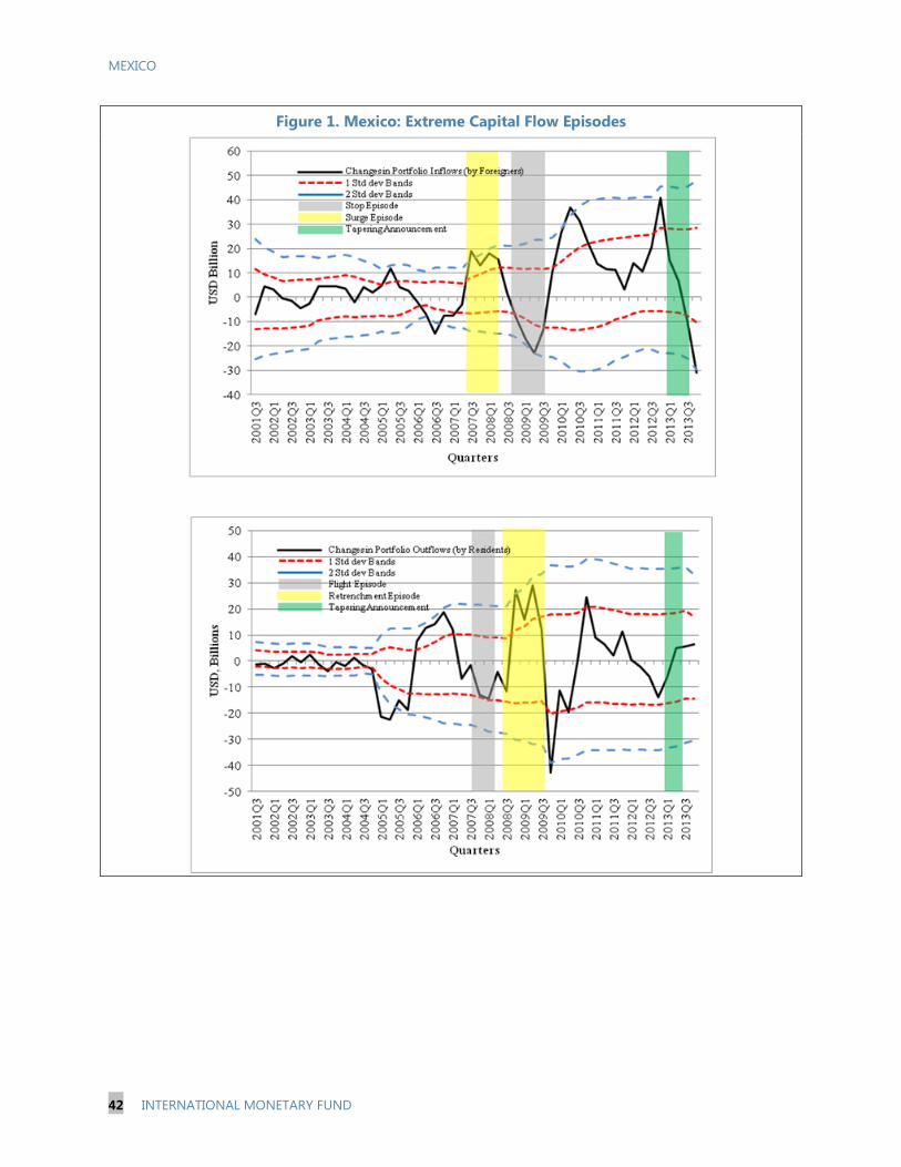
MEXICO
42 INTERNATIONAL MONETARY FUND
Figure 1. Mexico: Extreme Capital Flow Episodes
MEXICO
INTERNATIONAL MONETARY FUND 43
C. Behavior of Foreign and Domestic Mutual Funds in Mexico
In this section, we study the behavior of mutual funds active in Mexico during the periods of market
stress, especially shortly after the Fed tapering announcement in May 2013. We explore whether
foreign mutual fund investors are more inclined than domestic investors to sell as others are selling
(‘herding behavior’), and to buy when prices have risen (‘positive-feedback trading behavior’), relying
on two extensive fund flows datasets, one covers about 400 foreign mutual funds and another covers
540 Mexican mutual funds, at monthly frequency and with the latest data observation as recent as
April 2014. By doing so, we hope provide one plausible explanation for the large portfolio outflows
during the episodes of market stress, from the perspective of individual investor behaviors.
10. Herding in financial markets emerges when investors mimic other investors. Such
behavior can potentially destabilize financial markets, aggravate shocks, and lead to mispricing or
asset price bubbles. While herding can be the result of cognitive biases or of “heuristic”-based
decision making, it can also be a result of several other factors. For instance, herding may emerge if
there is asymmetric information sharing, which induces less-informed asset managers to follow their
possibly better-informed peers instead of relying on their own assessments, and in this context,
improving transparency may help reduce herding behavior (Kim and Wei, 2002; Bikhchandani,
Hirshleifer, and Welch, 1992). Herding may also occur if asset managers are evaluated against each
other (Scharfstein and Stein, 1990) or vis-à-vis similar benchmarks (Maug and Naik, 2011).
11. We use fund-level data in our analysis of herding and momentum trading behaviors.
To this end, we estimate the flow from each fund to Mexico using the country allocation data set
from the EPFR Global (see Box 2 for details). As of April 2014, there are a total of 375 foreign mutual
funds actively investing in Mexico, among which 112 are bond funds, and 263 are equity funds. Our
full sample is from January 2007 to April 2014, covering two “stress” episodes, namely the Global
Financial Crisis and the tapering announcement in May 2013, during which Mexico experienced
significant declines in gross portfolio inflows. In order to facilitate comparison between domestic
and foreign mutual funds active in Mexico, we use a shorter sample period (January 2011 to April
2014) for the analysis on momentum trading, as data on domestic mutual funds is only available
from January 2011.
12. We use two (related) measures to quantify co-movements in trading patterns for
funds—foreign or domestic—investing in Mexico:
A simple measure, defined by the proportion of all funds active in Mexico (in a particular month)
that are net sellers. This gives intuitive and indicative evidence of whether “correlated” selling
occurs at times of market stress.
A commonly used herding index originally introduced by Lakonshiok, Shleifer, and Vishy (1992).
This index assesses whether funds move in the same direction more often than one would
expect if they traded independently and randomly, and is computed as follows:
− − 𝐴
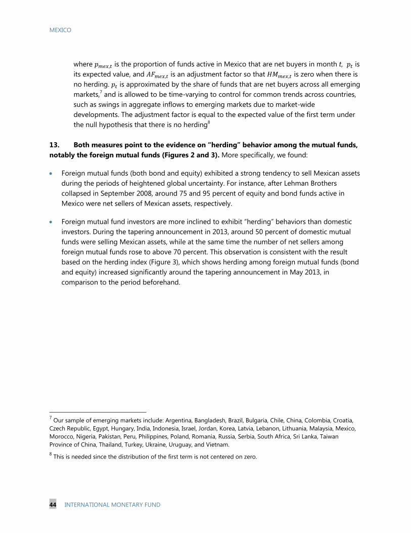
MEXICO
44 INTERNATIONAL MONETARY FUND
where is the proportion of funds active in Mexico that are net buyers in month t, is
its expected value, and 𝐴 is an adjustment factor so that is zero when there is
no herding. is approximated by the share of funds that are net buyers across all emerging
markets,7 and is allowed to be time-varying to control for common trends across countries,
such as swings in aggregate inflows to emerging markets due to market-wide
developments. The adjustment factor is equal to the expected value of the first term under
the null hypothesis that there is no herding8
13. Both measures point to the evidence on “herding” behavior among the mutual funds,
notably the foreign mutual funds (Figures 2 and 3). More specifically, we found:
Foreign mutual funds (both bond and equity) exhibited a strong tendency to sell Mexican assets
during the periods of heightened global uncertainty. For instance, after Lehman Brothers
collapsed in September 2008, around 75 and 95 percent of equity and bond funds active in
Mexico were net sellers of Mexican assets, respectively.
Foreign mutual fund investors are more inclined to exhibit “herding” behaviors than domestic
investors. During the tapering announcement in 2013, around 50 percent of domestic mutual
funds were selling Mexican assets, while at the same time the number of net sellers among
foreign mutual funds rose to above 70 percent. This observation is consistent with the result
based on the herding index (Figure 3), which shows herding among foreign mutual funds (bond
and equity) increased significantly around the tapering announcement in May 2013, in
comparison to the period beforehand.
7 Our sample of emerging markets include: Argentina, Bangladesh, Brazil, Bulgaria, Chile, China, Colombia, Croatia,
Czech Republic, Egypt, Hungary, India, Indonesia, Israel, Jordan, Korea, Latvia, Lebanon, Lithuania, Malaysia, Mexico,
Morocco, Nigeria, Pakistan, Peru, Philippines, Poland, Romania, Russia, Serbia, South Africa, Sri Lanka, Taiwan
Province of China, Thailand, Turkey, Ukraine, Uruguay, and Vietnam.
8 This is needed since the distribution of the first term is not centered on zero.
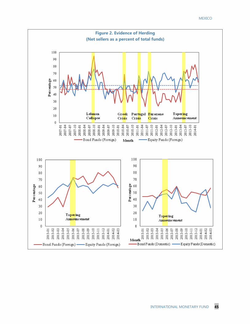
MEXICO
INTERNATIONAL MONETARY FUND 45
Figure 2. Evidence of Herding
(Net sellers as a percent of total funds)
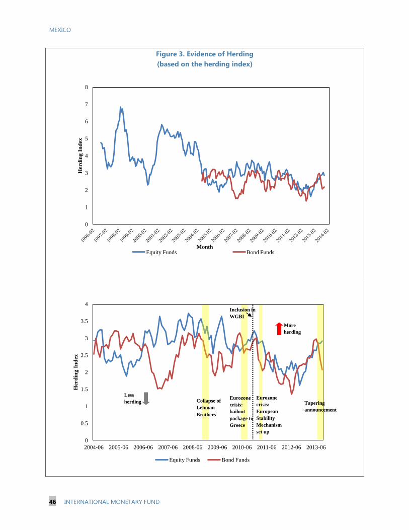
MEXICO
46 INTERNATIONAL MONETARY FUND
Figure 3. Evidence of Herding
(based on the herding index)
0
1
2
3
4
5
6
7
8
Her
din
g I
nd
ex
MonthEquity Funds Bond Funds
0
0.5
1
1.5
2
2.5
3
3.5
4
2004-06 2005-06 2006-06 2007-06 2008-06 2009-06 2010-06 2011-06 2012-06 2013-06
Her
din
g I
nd
ex
Equity Funds Bond Funds
Tapering
announcement
Collapse of
Lehman
Brothers
Eurozone
crisis:
bailout
package to
Greece
Eurozone
crisis:
European
Stability
Mechanism
set up
More
herding
Less
herding
Inclusion in
WGBI
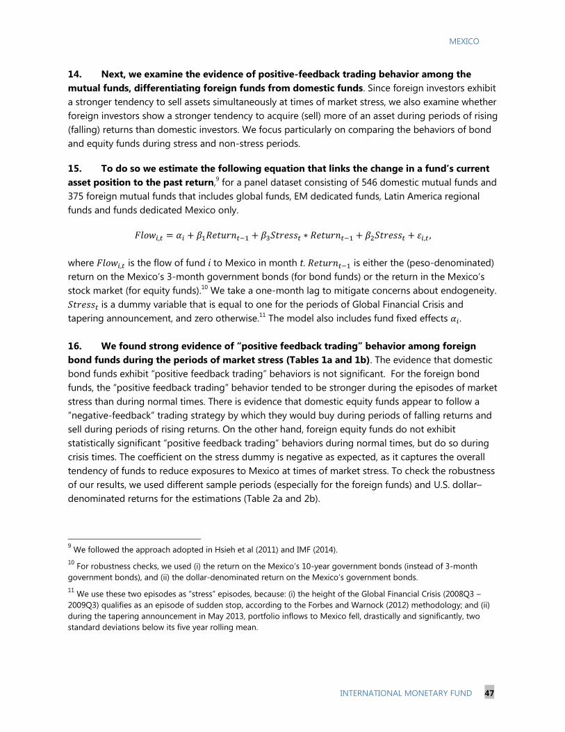
MEXICO
INTERNATIONAL MONETARY FUND 47
14. Next, we examine the evidence of positive-feedback trading behavior among the
mutual funds, differentiating foreign funds from domestic funds. Since foreign investors exhibit
a stronger tendency to sell assets simultaneously at times of market stress, we also examine whether
foreign investors show a stronger tendency to acquire (sell) more of an asset during periods of rising
(falling) returns than domestic investors. We focus particularly on comparing the behaviors of bond
and equity funds during stress and non-stress periods.
15. To do so we estimate the following equation that links the change in a fund’s current
asset position to the past return,9 for a panel dataset consisting of 546 domestic mutual funds and
375 foreign mutual funds that includes global funds, EM dedicated funds, Latin America regional
funds and funds dedicated Mexico only.
∗
where is the flow of fund i to Mexico in month t. is either the (peso-denominated)
return on the Mexico’s 3-month government bonds (for bond funds) or the return in the Mexico’s
stock market (for equity funds).10
We take a one-month lag to mitigate concerns about endogeneity.
is a dummy variable that is equal to one for the periods of Global Financial Crisis and
tapering announcement, and zero otherwise.11
The model also includes fund fixed effects .
16. We found strong evidence of “positive feedback trading” behavior among foreign
bond funds during the periods of market stress (Tables 1a and 1b). The evidence that domestic
bond funds exhibit “positive feedback trading” behaviors is not significant. For the foreign bond
funds, the “positive feedback trading” behavior tended to be stronger during the episodes of market
stress than during normal times. There is evidence that domestic equity funds appear to follow a
“negative-feedback” trading strategy by which they would buy during periods of falling returns and
sell during periods of rising returns. On the other hand, foreign equity funds do not exhibit
statistically significant “positive feedback trading” behaviors during normal times, but do so during
crisis times. The coefficient on the stress dummy is negative as expected, as it captures the overall
tendency of funds to reduce exposures to Mexico at times of market stress. To check the robustness
of our results, we used different sample periods (especially for the foreign funds) and U.S. dollar–
denominated returns for the estimations (Table 2a and 2b).
9 We followed the approach adopted in Hsieh et al (2011) and IMF (2014).
10 For robustness checks, we used (i) the return on the Mexico’s 10-year government bonds (instead of 3-month
government bonds), and (ii) the dollar-denominated return on the Mexico’s government bonds.
11 We use these two episodes as “stress” episodes, because: (i) the height of the Global Financial Crisis (2008Q3 –
2009Q3) qualifies as an episode of sudden stop, according to the Forbes and Warnock (2012) methodology; and (ii)
during the tapering announcement in May 2013, portfolio inflows to Mexico fell, drastically and significantly, two
standard deviations below its five year rolling mean.
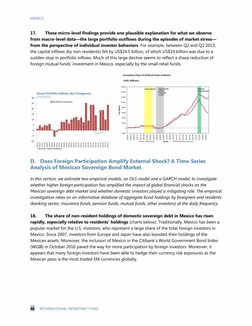
MEXICO
48 INTERNATIONAL MONETARY FUND
17. These micro-level findings provide one plausible explanation for what we observe
from macro-level data—the large portfolio outflows during the episodes of market stress—
from the perspective of individual investor behaviors. For example, between Q2 and Q1 2013,
the capital inflows (by non-residents) fell by US$24.5 billion, of which US$14 billion was due to a
sudden stop in portfolio inflows. Much of this large decline seems to reflect a sharp reduction of
foreign mutual funds’ investment in Mexico, especially by the small retail funds.
D. Does Foreign Participation Amplify External Shock? A Time-Series Analysis of Mexican Sovereign Bond Market
In this section, we estimate two empirical models, an OLS model and a GARCH model, to investigate
whether higher foreign participation has amplified the impact of global financial shocks on the
Mexican sovereign debt market and whether domestic investors played a mitigating role. The empirical
investigation relies on an informative database of aggregate bond holdings by foreigners and residents
(banking sector, insurance funds, pension funds, mutual funds, other investors) at the daily frequency.
18. The share of non-resident holdings of domestic sovereign debt in Mexico has risen
rapidly, especially relative to residents’ holdings (charts below). Traditionally, Mexico has been a
popular market for the U.S. investors, who represent a large share of the total foreign investors in
Mexico. Since 2007, investors from Europe and Japan have also boosted their holdings of the
Mexican assets. Moreover, the inclusion of Mexico in the Citibank’s World Government Bond Index
(WGIB) in October 2010 paved the way for more participation by foreign investors. Moreover, it
appears that many foreign investors have been able to hedge their currency risk exposures as the
Mexican peso is the most traded EM currencies globally.
-10
-5
0
5
10
15
20
25
30
2007Q
1
2007Q
2
2007Q
3
2007Q
4
2008Q
1
2008Q
2
2008Q
3
2008Q
4
2009Q
1
2009Q
2
2009Q
3
2009Q
4
2010Q
1
2010Q
2
2010Q
3
2010Q
4
2011Q
1
2011Q
2
2011Q
3
2011Q
4
2012Q
1
2012Q
2
2012Q
3
2012Q
4
2013Q
1
2013Q
2
2013Q
3
2013Q
4
2014Q
1
2014Q
2
Portfolio Investment
Gross Portfolio Inflows (by Foreigners)(USD, billions)
Sources: Haver Analytics
Cumulative Flows of All Bond Funds to Mexico
(USD, Millions)
-2000
0
2000
4000
6000
8000
10000
12000
14000
16000
20
06
/01
20
06
/05
20
06
/09
20
07
/01
20
07
/05
20
07
/09
20
08
/01
20
08
/05
20
08
/09
20
09
/01
20
09
/05
20
09
/09
20
10
/01
20
10
/05
20
10
/09
20
11
/01
20
11
/05
20
11
/09
20
12
/01
20
12
/05
20
12
/09
20
13
/01
20
13
/05
20
13
/09
20
14
/01
US
D M
illi
on
s
MonthEPFR Retail EPFR Institutional
Tapering
Announcement
Surge Episode Stop Episode
(Global
Financial
Crisis)
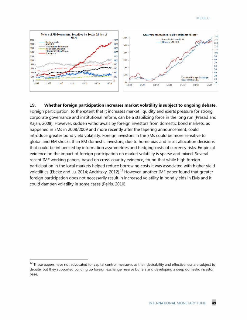
MEXICO
INTERNATIONAL MONETARY FUND 49
19. Whether foreign participation increases market volatility is subject to ongoing debate.
Foreign participation, to the extent that it increases market liquidity and exerts pressure for strong
corporate governance and institutional reform, can be a stabilizing force in the long run (Prasad and
Rajan, 2008). However, sudden withdrawals by foreign investors from domestic bond markets, as
happened in EMs in 2008/2009 and more recently after the tapering announcement, could
introduce greater bond yield volatility. Foreign investors in the EMs could be more sensitive to
global and EM shocks than EM domestic investors, due to home bias and asset allocation decisions
that could be influenced by information asymmetries and hedging costs of currency risks. Empirical
evidence on the impact of foreign participation on market volatility is sparse and mixed. Several
recent IMF working papers, based on cross-country evidence, found that while high foreign
participation in the local markets helped reduce borrowing costs it was associated with higher yield
volatilities (Ebeke and Lu, 2014; Andritzky, 2012).12
However, another IMF paper found that greater
foreign participation does not necessarily result in increased volatility in bond yields in EMs and it
could dampen volatility in some cases (Peiris, 2010).
12
These papers have not advocated for capital control measures as their desirability and effectiveness are subject to
debate, but they supported building up foreign exchange reserve buffers and developing a deep domestic investor
base.
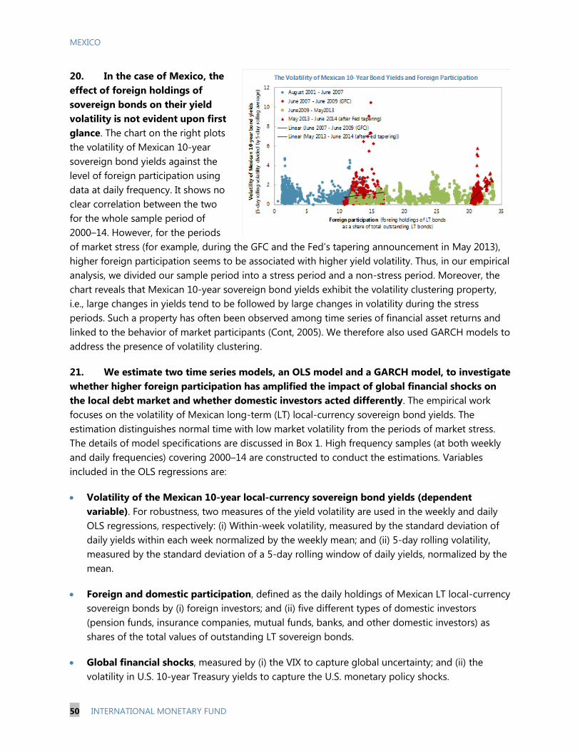
MEXICO
50 INTERNATIONAL MONETARY FUND
20. In the case of Mexico, the
effect of foreign holdings of
sovereign bonds on their yield
volatility is not evident upon first
glance. The chart on the right plots
the volatility of Mexican 10-year
sovereign bond yields against the
level of foreign participation using
data at daily frequency. It shows no
clear correlation between the two
for the whole sample period of
2000–14. However, for the periods
of market stress (for example, during the GFC and the Fed’s tapering announcement in May 2013),
higher foreign participation seems to be associated with higher yield volatility. Thus, in our empirical
analysis, we divided our sample period into a stress period and a non-stress period. Moreover, the
chart reveals that Mexican 10-year sovereign bond yields exhibit the volatility clustering property,
i.e., large changes in yields tend to be followed by large changes in volatility during the stress
periods. Such a property has often been observed among time series of financial asset returns and
linked to the behavior of market participants (Cont, 2005). We therefore also used GARCH models to
address the presence of volatility clustering.
21. We estimate two time series models, an OLS model and a GARCH model, to investigate
whether higher foreign participation has amplified the impact of global financial shocks on
the local debt market and whether domestic investors acted differently. The empirical work
focuses on the volatility of Mexican long-term (LT) local-currency sovereign bond yields. The
estimation distinguishes normal time with low market volatility from the periods of market stress.
The details of model specifications are discussed in Box 1. High frequency samples (at both weekly
and daily frequencies) covering 2000–14 are constructed to conduct the estimations. Variables
included in the OLS regressions are:
Volatility of the Mexican 10-year local-currency sovereign bond yields (dependent
variable). For robustness, two measures of the yield volatility are used in the weekly and daily
OLS regressions, respectively: (i) Within-week volatility, measured by the standard deviation of
daily yields within each week normalized by the weekly mean; and (ii) 5-day rolling volatility,
measured by the standard deviation of a 5-day rolling window of daily yields, normalized by the
mean.
Foreign and domestic participation, defined as the daily holdings of Mexican LT local-currency
sovereign bonds by (i) foreign investors; and (ii) five different types of domestic investors
(pension funds, insurance companies, mutual funds, banks, and other domestic investors) as
shares of the total values of outstanding LT sovereign bonds.
Global financial shocks, measured by (i) the VIX to capture global uncertainty; and (ii) the
volatility in U.S. 10-year Treasury yields to capture the U.S. monetary policy shocks.
MEXICO
INTERNATIONAL MONETARY FUND 51
Domestic variables: official international reserves (weekly, excluding gold), peso/US dollar
exchange rate (daily), and interbank interest rate (daily).13
Variables included in the (daily) multivariate GARCH models are the changes in the Mexican
10-year local-currency sovereign bond yields, the changes in the Mexican stock market returns
(dependent variables), and the explanatory variables included in the daily OLS regressions.
22. The empirical results of the OLS regressions and multivariate GARCH models are
presented in Tables 3a, 3b, 4a, and 4b. Several interesting results emerge:
First, foreign participation tends to amplify the impact of global financial shocks on the
volatility of Mexican sovereign bond yields, notably during the periods of market stress.
Results from both the OLS regressions and the multivariate GARCH models are consistent and
robust across all specifications. This implies that the foreign participation in the local-currency
bond market can make the market more susceptible to adverse shifts in the market sentiment
caused by global financial shocks. From finance theory, due to information asymmetry or
currency risks, local-currency assets tend to have larger risks for foreign investors than for
domestic investors when global risk aversion rises or global liquidity tightens. As a result, foreign
investors’ holdings of local-currency assets could be more sensitive to global financial conditions
than local investors’ holdings, generating “extra” volatility in local markets. The results of the
GARCH regressions show that higher participation by foreign investors in the Mbono market
heightens the sensivity of the volatility of the 10-year Mbono yield, without necessarily affecting
the level of the Mbono yield, to a shock to the VIX. At the same time, increased foreign
participation does make both the level and volatility of the Mbono yield more sensitive shocks
to the yield on 10-year US Treasuries. This discrepancy could reflect the fact that—over this
sample period—surges in the VIX were often associated decline in the level of the yield on the
10-year US Treasuries, since this asset was viewed as the safe asset.
Second, domestic investors in the sovereign bond market played some mitigating role,
but the empirical evidence was mixed, depending on the type of investors and the nature
of the global shocks. In particular, banks seem to amplify the impact of global financial shocks
on domestic yield volatility during normal times across all specifications, but their role during
stress periods seems to be unclear. In addition, the results based on the OLS regressions find
that domestic pension funds and banks seem to dampen the impact of VIX shock during stress
periods, but there is no significant and robust evidence that the insurance sector or the mutual
funds play any mitigating or amplifying role during stress periods. Moreover, the mitigating role
of the pension funds no longer holds if the shock is to the U.S. 10-year Treasury yields. These
13
The 28 day TIIE interbank equilibrium rate is used as the interbank interest rate to capture domestic monetary
policy. The first-order differences of the reserves and interest rates, as well as the first-order differences of log
exchange rates are used in the regressions.
MEXICO
52 INTERNATIONAL MONETARY FUND
mixed results tend to suggest that domestic investors are not significantly different from each
other, and their behaviors would depend on the nature of the global financial shocks.14
23. These results are robust to the choices of dependent and independent variables. For
the dependent variable, another volatility measure using the exchange rates rather than the
sovereign bond yields is also used in the OLS regressions, and the main (qualitative) result that
foreign participation tends to amplify global financial shocks does not change. For the independent
variables, we replace the shares of respective investors in the interaction terms by their first-order
differences, and the main results still hold.
E. Concluding Remarks
24. The size and volatility of gross capital inflows (particularly portfolio inflows) to Mexico
have increased in recent years. Mexico remains vulnerable to global financial shocks, given its
globally integrated financial markets. A resurgence of investor uncertainty triggered by an earlier or
sharper-than-expected rise in U.S. interest rates (for example due to an unexpected rise in inflation
or a decompression of U.S. term premia) presents a distinct risk in the near term. As our analysis of
the Fed tapering incident in May 2013 has shown, such a shock could lead to a significant portfolio
capital outflows from Mexico, resulted in high volatility in bond prices. A protracted period of
financial market volatility could affect the confidence of long-term investors and threaten the
ongoing progress on the implementation of structural reforms.
25. This paper investigates the behaviors of foreign and domestic investors, especially
during the periods of market stress. More specifically, relying on three approaches using both
macro- and micro-level data, our empirical investigations suggest that foreign and domestic
investors do seem to behave differently. We found that foreign mutual fund investors exhibited
potentially destabilizing trading behaviors that could contribute to market volatility. For examples,
they tended to sell as others are selling (‘herding behavior’) and follow a “positive-feedback trading”
strategy (i.e. buy high and sell low). We did not find significant evidence indicating that domestic
mutual funds behaved similarly. Moreover, our study of the Mexican sovereign bond markets
suggests that foreign participation tended to amplify the impact of global financial shocks, notably
in periods of market stress. Domestic institutional investors played some mitigating role, but the
evidence is mixed and depends on the nature of the external shocks.
26. These results imply that policy credibility will continue to be key to maintain market
confidence at times of stress. Mexico has a strong policy framework,15
with sound public finances,
low and stable inflation, a sustainable external sector position, and a healthy banking system. It also
14
Our result is consistent with the finding in the IMF’s Regional Economic Outlook: Western Hemisphere (April 2014)
that a shock in VIX (which may reflect global uncertainty) can have diffenrt impact from a shock in US interest rate.
15 Monetary policy is guided by an inflation targeting framework under a flexible exchange rate, and fiscal policy is
anchored by a fiscal responsibility law.

MEXICO
INTERNATIONAL MONETARY FUND 53
has one of the highest credit ratings among emerging markets. These strong fundamentals have
helped attract foreigner investors and maintain a strong demand from local investors, especially
during the periods of market stress. For example, during the GFC local investors reduced their
holdings of foreign assets and brought local assets when foreigners left Mexican market. The
situation was very different during the Mexican peso crisis in 2004, when both foreign and local
investors deserted the country amid the great domestic policy uncertainty.
27. Country insurance against global risks may be necessary. While the exchange rate
flexibility acted as an effective shock absorber, the high level of reserves has provided a useful buffer
against temporary stress in foreign exchange markets.16
The FCL arrangement, which the authorities
continue to treat as precautionary, was an important complement to reserve buffers, providing
additional protection against tail risks. For instance, in the aftermath of the announcements by
Federal Reserve Board members about imminent tapering, capital inflows by non-residents dropped
by US$24.5 billion from Q1to Q2 2013. The exchange rate depreciated by 8 percent. Both of these
developments were quickly reversed, as investors began differentiating between emerging markets,
and Mexico stood out for its strong macroeconomic fundamentals, but also its large foreign
exchange buffer, notably when including the FCL.
28. Finally, a deep and diverse domestic investor base is important as well. Mexico has
benefited from an expanding and diverse local investor base, thanks to pension reforms and the
establishment of insurance and mutual fund industries. These investors could play a more important
stabilizing role to the Mexican financial markets, for example, by improving liquidity in the
secondary markets for government securities.
16
International reserves stand at about US$190bn as of June 2014.
8
9
10
11
12
13
14
15
16
17
18
-10
-5
0
5
10
15
20
25
30
2007 2008 2009 2010 2011 2012 2013 2014
Portfolio investment Peso/USD exchange rate (RHS)
Gross Portfolio Inflows by Foreigners(USD, billions)
Source: Haver Analytics.
Fed tapering talk
0
20
40
60
80
100
120
140
0
20
40
60
80
100
120
140
Ven
ezu
ela
Pan
am
a
So
uth
Afr
ica
Mexic
o
Ind
on
esi
a
Jam
aic
a
Po
lan
d
Bra
zil
Ch
ile
Lit
hu
an
ia
El S
alv
ad
or
Tu
rkey
Do
m. R
ep
.
Arg
en
tin
a
Pakis
tan
Co
lom
bia
Cro
ati
a
Th
ailan
d
FCL Reserves to Portfolio Investment
In percent
Mexico: 38.1% plus 15.4% of FCL
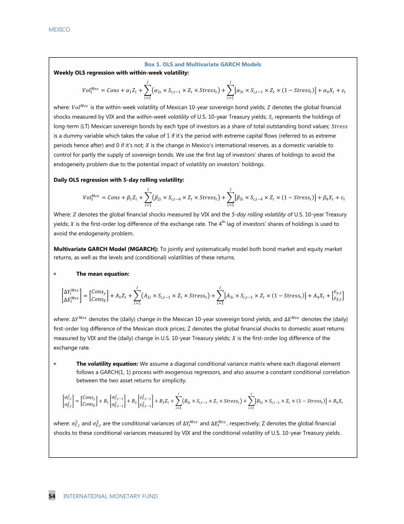
MEXICO
54 INTERNATIONAL MONETARY FUND
Table 1a. Bond Funds: Evidence of Positive Feedback Trading Behavior
Explanatory Variables Domestic Funds Foreign Funds
(1) (2) (1) (2)
Fund Flow Fund Flow Fund Flow Fund Flow
Lagged Mex 3-month bond yield 0.00726 0.00628 0.00725*** 0.00660***
(0.00541) (0.00543) (0.000765) (0.000770)
Lagged bond yield * Stress 0.00481** 0.0171***
(0.00225) (0.00567)
Stress -0.0177* -0.0677***
(0.00945) (0.0229)
Constant -0.0205 -0.0166 -0.0288*** -0.0260***
(0.0220) (0.0221) (0.00319) (0.00321)
Fund Fixed Effects YES YES YES YES
Number of Observations 20202 20202 3422 3422
R-squared 0.019 0.019 0.172 0.178
Standard errors (robust) in parentheses *p<0.10 **p<0.50 ***p<0.01
Sample size: 2011 January – 2014 March (stress episode: tapering announcement)
Table 1b. Equity Funds: Evidence of Positive Feedback Trading Behavior
Explanatory Variables Domestic Funds Foreign Funds
(1) (2) (1) (2)
Fund Flow Fund Flow Fund Flow Fund Flow
Lagged stock market return -0.0211* -0.0269** 0.00228** 0.000615
(0.0115) (0.0123) (0.00113) (0.00105)
Lagged stock market return * Stress -0.0986* 0.0138**
(0.0517) (0.00657)
𝑉 𝑥 = + 1𝑍 + 2 × , −1 × 𝑍 ×
=1
+ 3 × , −1 × 𝑍 × 1 −
=1
+ 4𝑋 +
𝑉 𝑥 = + 1𝑍 + 2 × , −4 × 𝑍 ×
=1
+ 3 × , −4 × 𝑍 × 1 −
=1
+ 4𝑋 +
𝑌
𝑥
𝑥 =
+ 𝐴1𝑍 + 𝐴2 × , −1 × 𝑍 ×
=1
+ 𝐴3 × , −1 × 𝑍 × 1 −
=1
+ 𝐴4𝑋 + ,
,
𝜎𝑌,
2
𝜎 , 2 =
+ 𝐵1 𝜎𝑌, −1
2
𝜎 , −12 + 𝐵2
𝑌, −12
, −12 + 𝐵3𝑍 + 𝐵4 × , −1 × 𝑍 ×
=1
+ 𝐵5 × , −1 × 𝑍 × 1 −
=1
+ 𝐵6𝑋
Box 1. OLS and Multivariate GARCH Models
Weekly OLS regression with within-week volatility:
where: 𝑉 𝑥 is the within-week volatility of Mexican 10-year sovereign bond yields; 𝑍 denotes the global financial
shocks measured by VIX and the within-week volatility of U.S. 10-year Treasury yields; represents the holdings of
long-term (LT) Mexican sovereign bonds by each type of investors as a share of total outstanding bond values;
is a dummy variable which takes the value of 1 if it’s the period with extreme capital flows (referred to as extreme
periods hence after) and 0 if it’s not; 𝑋 is the change in Mexico’s international reserves, as a domestic variable to
control for partly the supply of sovereign bonds. We use the first lag of investors’ shares of holdings to avoid the
endogeneity problem due to the potential impact of volatility on investors’ holdings.
Daily OLS regression with 5-day rolling volatility:
Where: 𝑍 denotes the global financial shocks measured by VIX and the 5-day rolling volatility of U.S. 10-year Treasury
yields; 𝑋 is the first-order log difference of the exchange rate. The 4th
lag of investors’ shares of holdings is used to
avoid the endogeneity problem.
Multivariate GARCH Model (MGARCH): To jointly and systematically model both bond market and equity market
returns, as well as the levels and (conditional) volatilities of these returns.
The mean equation:
where: 𝑌 𝑥 denotes the (daily) change in the Mexican 10-year sovereign bond yields, and 𝑥 denotes the (daily)
first-order log difference of the Mexican stock prices; Z denotes the global financial shocks to domestic asset returns
measured by VIX and the (daily) change in U.S. 10-year Treasury yields; 𝑋 is the first-order log difference of the
exchange rate.
The volatility equation: We assume a diagonal conditional variance matrix where each diagonal element
follows a GARCH(1, 1) process with exogenous regressors, and also assume a constant conditional correlation
between the two asset returns for simplicity.
where: 𝜎𝑌, 2 and 𝜎 ,
2 are the conditional variances of 𝑌 𝑥 and
𝑥 , respectively; Z denotes the global financial
shocks to these conditional variances measured by VIX and the conditional volatility of U.S. 10-year Treasury yields.
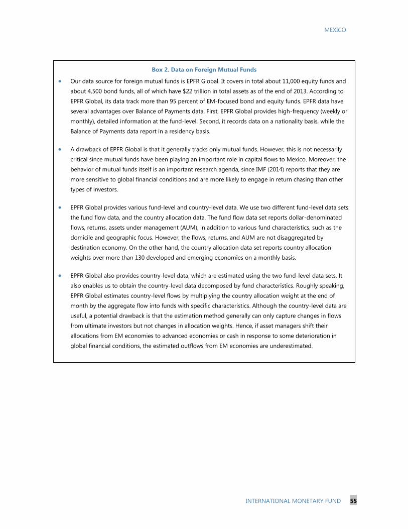
MEXICO
INTERNATIONAL MONETARY FUND 55
Box 2. Data on Foreign Mutual Funds
Our data source for foreign mutual funds is EPFR Global. It covers in total about 11,000 equity funds and
about 4,500 bond funds, all of which have $22 trillion in total assets as of the end of 2013. According to
EPFR Global, its data track more than 95 percent of EM-focused bond and equity funds. EPFR data have
several advantages over Balance of Payments data. First, EPFR Global provides high-frequency (weekly or
monthly), detailed information at the fund-level. Second, it records data on a nationality basis, while the
Balance of Payments data report in a residency basis.
A drawback of EPFR Global is that it generally tracks only mutual funds. However, this is not necessarily
critical since mutual funds have been playing an important role in capital flows to Mexico. Moreover, the
behavior of mutual funds itself is an important research agenda, since IMF (2014) reports that they are
more sensitive to global financial conditions and are more likely to engage in return chasing than other
types of investors.
EPFR Global provides various fund-level and country-level data. We use two different fund-level data sets:
the fund flow data, and the country allocation data. The fund flow data set reports dollar-denominated
flows, returns, assets under management (AUM), in addition to various fund characteristics, such as the
domicile and geographic focus. However, the flows, returns, and AUM are not disaggregated by
destination economy. On the other hand, the country allocation data set reports country allocation
weights over more than 130 developed and emerging economies on a monthly basis.
EPFR Global also provides country-level data, which are estimated using the two fund-level data sets. It
also enables us to obtain the country-level data decomposed by fund characteristics. Roughly speaking,
EPFR Global estimates country-level flows by multiplying the country allocation weight at the end of
month by the aggregate flow into funds with specific characteristics. Although the country-level data are
useful, a potential drawback is that the estimation method generally can only capture changes in flows
from ultimate investors but not changes in allocation weights. Hence, if asset managers shift their
allocations from EM economies to advanced economies or cash in response to some deterioration in
global financial conditions, the estimated outflows from EM economies are underestimated.
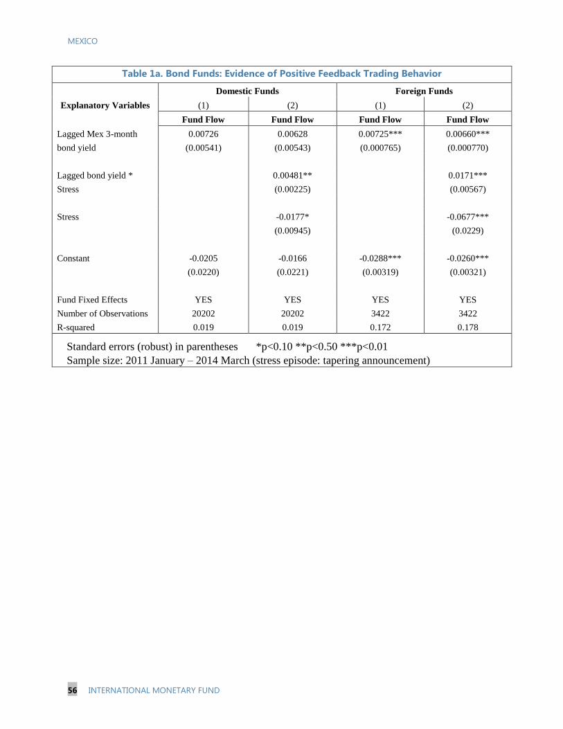
MEXICO
56 INTERNATIONAL MONETARY FUND
Table 1a. Bond Funds: Evidence of Positive Feedback Trading Behavior
Explanatory Variables
Domestic Funds Foreign Funds
(1) (2) (1) (2)
Fund Flow Fund Flow Fund Flow Fund Flow
Lagged Mex 3-month
bond yield
0.00726 0.00628 0.00725*** 0.00660***
(0.00541) (0.00543) (0.000765) (0.000770)
Lagged bond yield *
Stress
0.00481** 0.0171***
(0.00225) (0.00567)
Stress -0.0177* -0.0677***
(0.00945) (0.0229)
Constant -0.0205 -0.0166 -0.0288*** -0.0260***
(0.0220) (0.0221) (0.00319) (0.00321)
Fund Fixed Effects YES YES YES YES
Number of Observations 20202 20202 3422 3422
R-squared 0.019 0.019 0.172 0.178
Standard errors (robust) in parentheses *p<0.10 **p<0.50 ***p<0.01
Sample size: 2011 January – 2014 March (stress episode: tapering announcement)
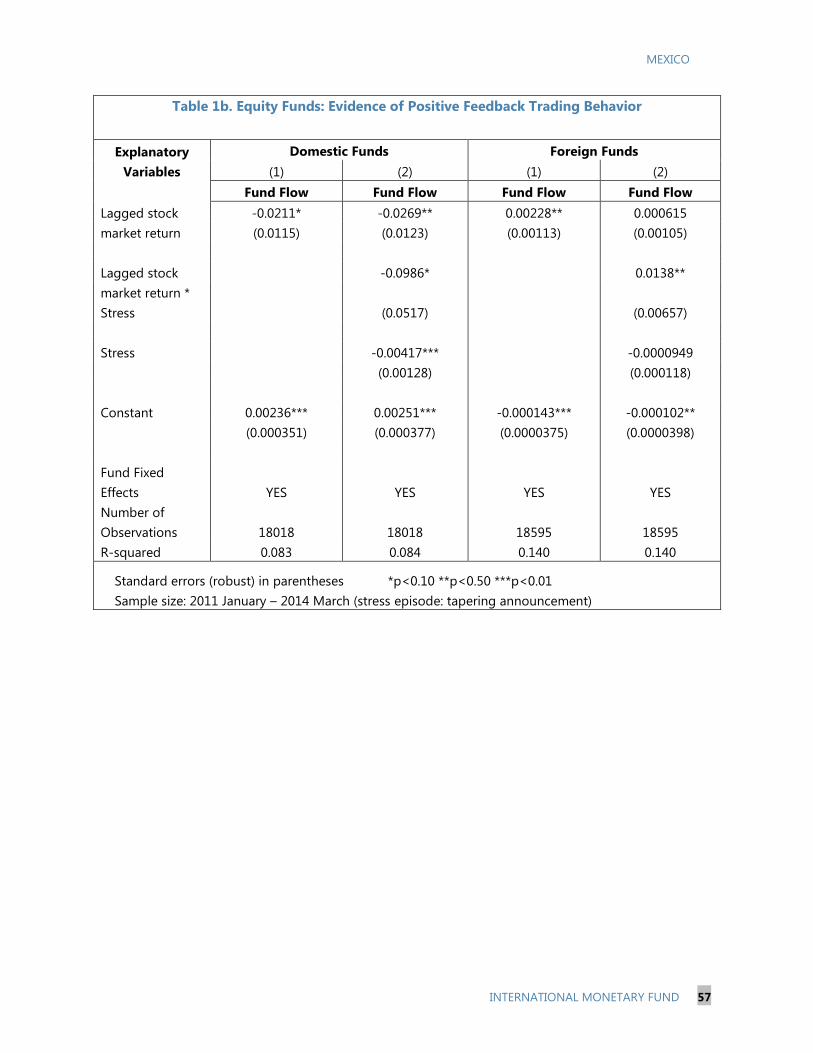
MEXICO
INTERNATIONAL MONETARY FUND 57
Table 1b. Equity Funds: Evidence of Positive Feedback Trading Behavior
Explanatory
Variables
Domestic Funds Foreign Funds
(1) (2) (1) (2)
Fund Flow Fund Flow Fund Flow Fund Flow
Lagged stock
market return
-0.0211* -0.0269** 0.00228** 0.000615
(0.0115) (0.0123) (0.00113) (0.00105)
Lagged stock
market return *
Stress
-0.0986* 0.0138**
(0.0517) (0.00657)
Stress -0.00417*** -0.0000949
(0.00128) (0.000118)
Constant 0.00236*** 0.00251*** -0.000143*** -0.000102**
(0.000351) (0.000377) (0.0000375) (0.0000398)
Fund Fixed
Effects YES YES YES YES
Number of
Observations 18018 18018 18595 18595
R-squared 0.083 0.084 0.140 0.140
Standard errors (robust) in parentheses *p<0.10 **p<0.50 ***p<0.01
Sample size: 2011 January – 2014 March (stress episode: tapering announcement)
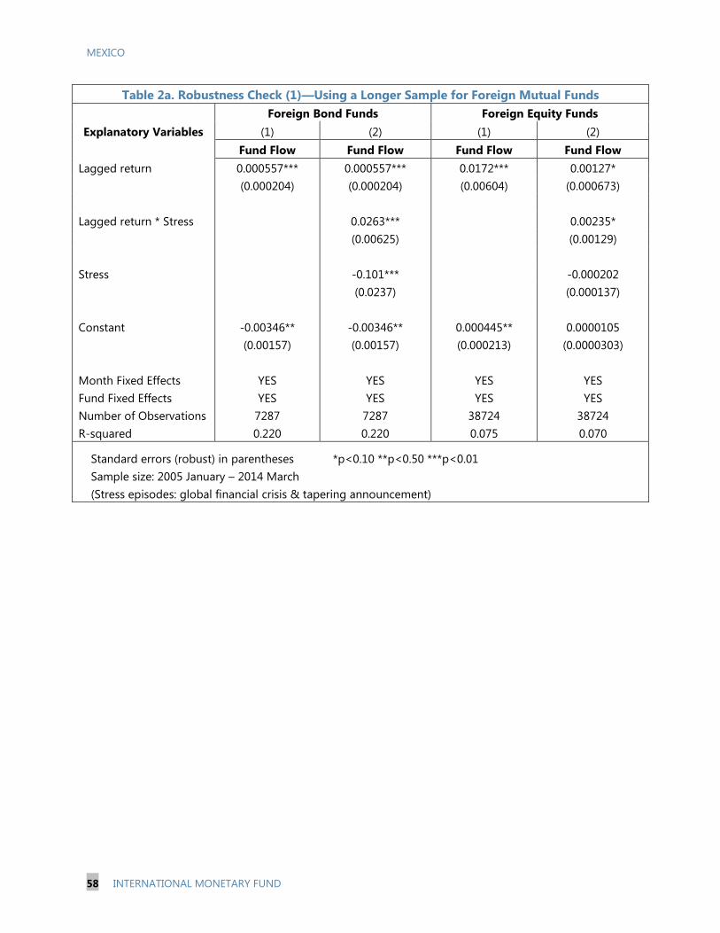
MEXICO
58 INTERNATIONAL MONETARY FUND
Table 2a. Robustness Check (1)—Using a Longer Sample for Foreign Mutual Funds
Explanatory Variables
Foreign Bond Funds Foreign Equity Funds
(1) (2) (1) (2)
Fund Flow Fund Flow Fund Flow Fund Flow
Lagged return 0.000557*** 0.000557*** 0.0172*** 0.00127*
(0.000204) (0.000204) (0.00604) (0.000673)
Lagged return * Stress 0.0263*** 0.00235*
(0.00625) (0.00129)
Stress -0.101*** -0.000202
(0.0237) (0.000137)
Constant -0.00346** -0.00346** 0.000445** 0.0000105
(0.00157) (0.00157) (0.000213) (0.0000303)
Month Fixed Effects YES YES YES YES
Fund Fixed Effects YES YES YES YES
Number of Observations 7287 7287 38724 38724
R-squared 0.220 0.220 0.075 0.070
Standard errors (robust) in parentheses *p<0.10 **p<0.50 ***p<0.01
Sample size: 2005 January – 2014 March
(Stress episodes: global financial crisis & tapering announcement)
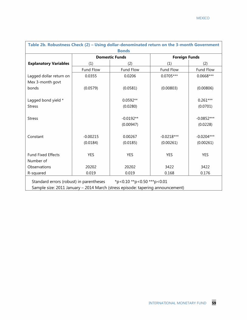
MEXICO
INTERNATIONAL MONETARY FUND 59
Table 2b. Robustness Check (2) – Using dollar-denominated return on the 3-month Government
Bonds
Explanatory Variables
Domestic Funds Foreign Funds
(1) (2) (1) (2)
Fund Flow Fund Flow Fund Flow Fund Flow
Lagged dollar return on
Mex 3-month govt
bonds
0.0355 0.0206 0.0705*** 0.0668***
(0.0579) (0.0581) (0.00803) (0.00806)
Lagged bond yield *
Stress
0.0592** 0.261***
(0.0280) (0.0701)
Stress -0.0192** -0.0852***
(0.00947) (0.0228)
Constant -0.00215 0.00267 -0.0218*** -0.0204***
(0.0184) (0.0185) (0.00261) (0.00261)
Fund Fixed Effects YES YES YES YES
Number of
Observations 20202 20202 3422 3422
R-squared 0.019 0.019 0.168 0.176
Standard errors (robust) in parentheses *p<0.10 **p<0.50 ***p<0.01
Sample size: 2011 January – 2014 March (stress episode: tapering announcement)
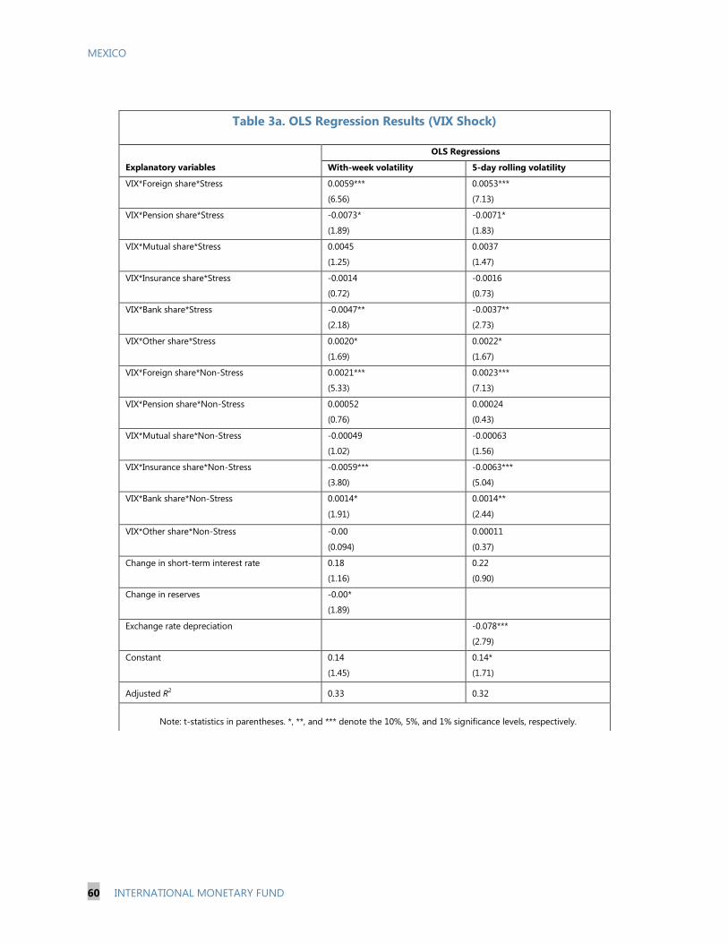
MEXICO
60 INTERNATIONAL MONETARY FUND
Table 3a. OLS Regression Results (VIX Shock)
Explanatory variables
OLS Regressions
With-week volatility 5-day rolling volatility
VIX*Foreign share*Stress 0.0059***
(6.56)
0.0053***
(7.13)
VIX*Pension share*Stress -0.0073*
(1.89)
-0.0071*
(1.83)
VIX*Mutual share*Stress 0.0045
(1.25)
0.0037
(1.47)
VIX*Insurance share*Stress -0.0014
(0.72)
-0.0016
(0.73)
VIX*Bank share*Stress -0.0047**
(2.18)
-0.0037**
(2.73)
VIX*Other share*Stress 0.0020*
(1.69)
0.0022*
(1.67)
VIX*Foreign share*Non-Stress 0.0021***
(5.33)
0.0023***
(7.13)
VIX*Pension share*Non-Stress 0.00052
(0.76)
0.00024
(0.43)
VIX*Mutual share*Non-Stress -0.00049
(1.02)
-0.00063
(1.56)
VIX*Insurance share*Non-Stress -0.0059***
(3.80)
-0.0063***
(5.04)
VIX*Bank share*Non-Stress 0.0014*
(1.91)
0.0014**
(2.44)
VIX*Other share*Non-Stress -0.00
(0.094)
0.00011
(0.37)
Change in short-term interest rate
0.18
(1.16)
0.22
(0.90)
Change in reserves -0.00*
(1.89)
Exchange rate depreciation -0.078***
(2.79)
Constant 0.14
(1.45)
0.14*
(1.71)
Adjusted R2 0.33 0.32
Note: t-statistics in parentheses. *, **, and *** denote the 10%, 5%, and 1% significance levels, respectively.
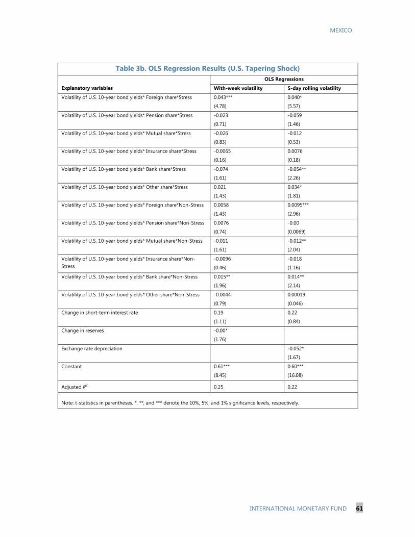
MEXICO
INTERNATIONAL MONETARY FUND 61
Table 3b. OLS Regression Results (U.S. Tapering Shock)
Explanatory variables
OLS Regressions
With-week volatility 5-day rolling volatility
Volatility of U.S. 10-year bond yields* Foreign share*Stress 0.043***
(4.78)
0.040*
(5.57)
Volatility of U.S. 10-year bond yields* Pension share*Stress -0.023
(0.71)
-0.059
(1.46)
Volatility of U.S. 10-year bond yields* Mutual share*Stress -0.026
(0.83)
-0.012
(0.53)
Volatility of U.S. 10-year bond yields* Insurance share*Stress -0.0065
(0.16)
0.0076
(0.18)
Volatility of U.S. 10-year bond yields* Bank share*Stress -0.074
(1.61)
-0.054**
(2.26)
Volatility of U.S. 10-year bond yields* Other share*Stress 0.021
(1.43)
0.034*
(1.81)
Volatility of U.S. 10-year bond yields* Foreign share*Non-Stress 0.0058
(1.43)
0.0095***
(2.96)
Volatility of U.S. 10-year bond yields* Pension share*Non-Stress 0.0076
(0.74)
-0.00
(0.0069)
Volatility of U.S. 10-year bond yields* Mutual share*Non-Stress -0.011
(1.61)
-0.012**
(2.04)
Volatility of U.S. 10-year bond yields* Insurance share*Non-
Stress
-0.0096
(0.46)
-0.018
(1.16)
Volatility of U.S. 10-year bond yields* Bank share*Non-Stress 0.015**
(1.96)
0.014**
(2.14)
Volatility of U.S. 10-year bond yields* Other share*Non-Stress -0.0044
(0.79)
0.00019
(0.046)
Change in short-term interest rate
0.19
(1.11)
0.22
(0.84)
Change in reserves -0.00*
(1.76)
Exchange rate depreciation -0.052*
(1.67)
Constant 0.61***
(8.45)
0.60***
(16.08)
Adjusted R2 0.25 0.22
Note: t-statistics in parentheses. *, **, and *** denote the 10%, 5%, and 1% significance levels, respectively.
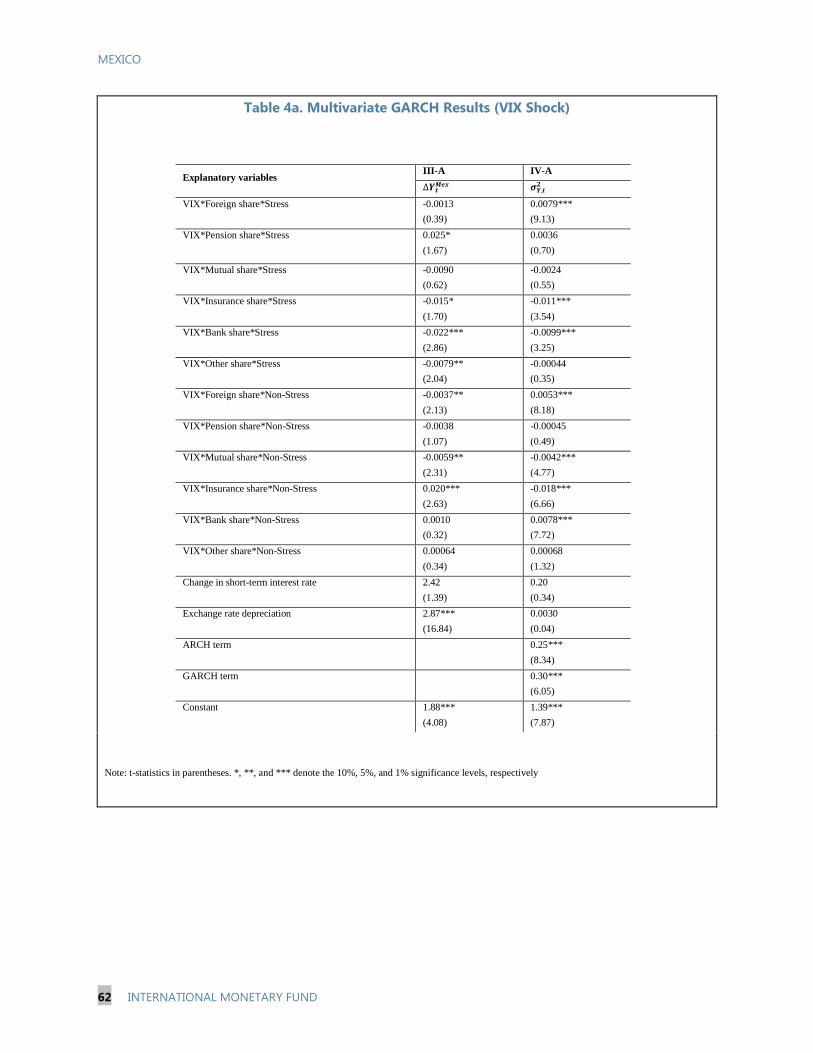
MEXICO
62 INTERNATIONAL MONETARY FUND
Table 4a. Multivariate GARCH Results (VIX Shock)
Note: t-statistics in parentheses. *, **, and *** denote the 10%, 5%, and 1% significance levels, respectively
Explanatory variables III-A IV-A
𝒀 𝑴𝒆𝒙 𝝈𝒀,
VIX*Foreign share*Stress -0.0013
(0.39)
0.0079***
(9.13)
VIX*Pension share*Stress 0.025*
(1.67)
0.0036
(0.70)
VIX*Mutual share*Stress -0.0090
(0.62)
-0.0024
(0.55)
VIX*Insurance share*Stress -0.015*
(1.70)
-0.011***
(3.54)
VIX*Bank share*Stress -0.022***
(2.86)
-0.0099***
(3.25)
VIX*Other share*Stress -0.0079**
(2.04)
-0.00044
(0.35)
VIX*Foreign share*Non-Stress -0.0037**
(2.13)
0.0053***
(8.18)
VIX*Pension share*Non-Stress -0.0038
(1.07)
-0.00045
(0.49)
VIX*Mutual share*Non-Stress -0.0059**
(2.31)
-0.0042***
(4.77)
VIX*Insurance share*Non-Stress 0.020***
(2.63)
-0.018***
(6.66)
VIX*Bank share*Non-Stress 0.0010
(0.32)
0.0078***
(7.72)
VIX*Other share*Non-Stress 0.00064
(0.34)
0.00068
(1.32)
Change in short-term interest rate
2.42
(1.39)
0.20
(0.34)
Exchange rate depreciation 2.87***
(16.84)
0.0030
(0.04)
ARCH term 0.25***
(8.34)
GARCH term 0.30***
(6.05)
Constant 1.88***
(4.08)
1.39***
(7.87)
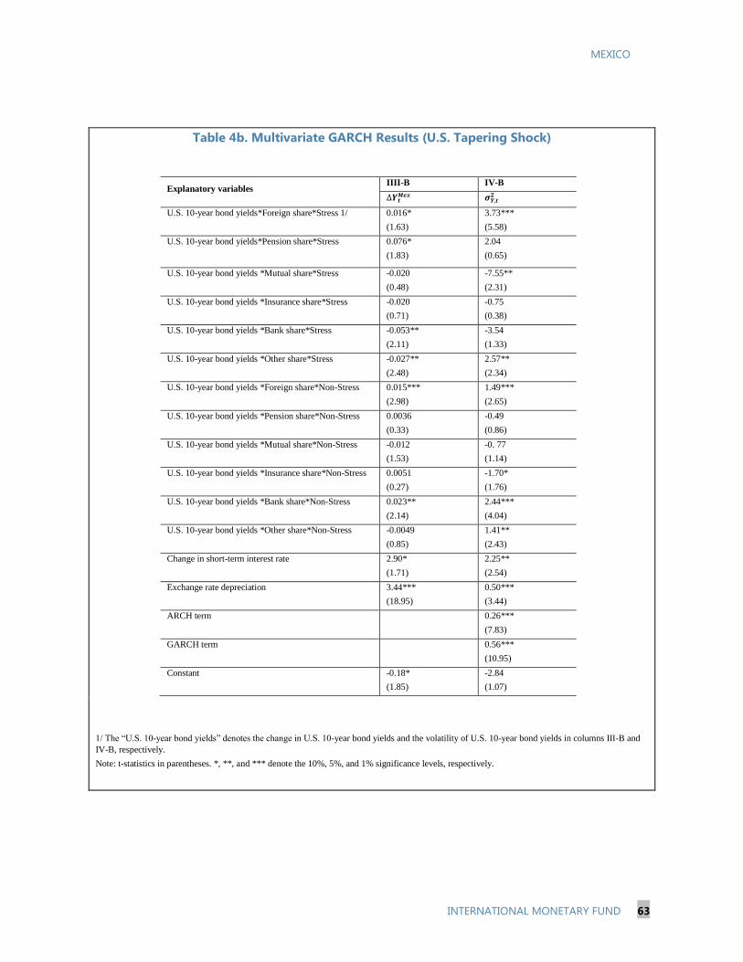
MEXICO
INTERNATIONAL MONETARY FUND 63
Table 4b. Multivariate GARCH Results (U.S. Tapering Shock)
1/ The “U.S. 10-year bond yields” denotes the change in U.S. 10-year bond yields and the volatility of U.S. 10-year bond yields in columns III-B and
IV-B, respectively.
Note: t-statistics in parentheses. *, **, and *** denote the 10%, 5%, and 1% significance levels, respectively.
Explanatory variables IIII-B IV-B
𝒀 𝑴𝒆𝒙 𝝈𝒀,
U.S. 10-year bond yields*Foreign share*Stress 1/ 0.016*
(1.63)
3.73***
(5.58)
U.S. 10-year bond yields*Pension share*Stress 0.076*
(1.83)
2.04
(0.65)
U.S. 10-year bond yields *Mutual share*Stress -0.020
(0.48)
-7.55**
(2.31)
U.S. 10-year bond yields *Insurance share*Stress -0.020
(0.71)
-0.75
(0.38)
U.S. 10-year bond yields *Bank share*Stress -0.053**
(2.11)
-3.54
(1.33)
U.S. 10-year bond yields *Other share*Stress -0.027**
(2.48)
2.57**
(2.34)
U.S. 10-year bond yields *Foreign share*Non-Stress 0.015***
(2.98)
1.49***
(2.65)
U.S. 10-year bond yields *Pension share*Non-Stress 0.0036
(0.33)
-0.49
(0.86)
U.S. 10-year bond yields *Mutual share*Non-Stress -0.012
(1.53)
-0. 77
(1.14)
U.S. 10-year bond yields *Insurance share*Non-Stress 0.0051
(0.27)
-1.70*
(1.76)
U.S. 10-year bond yields *Bank share*Non-Stress 0.023**
(2.14)
2.44***
(4.04)
U.S. 10-year bond yields *Other share*Non-Stress -0.0049
(0.85)
1.41**
(2.43)
Change in short-term interest rate
2.90*
(1.71)
2.25**
(2.54)
Exchange rate depreciation 3.44***
(18.95)
0.50***
(3.44)
ARCH term 0.26***
(7.83)
GARCH term 0.56***
(10.95)
Constant -0.18*
(1.85)
-2.84
(1.07)
MEXICO
64 INTERNATIONAL MONETARY FUND
References
Andritzky, Jochen R. (2012), “Government Bonds and Their Investors: What Are the Facts and Do
They Matter?” IMF Working Papers, WP/12/158, June.
Bikhchandani, Sushil, David Hirshleifer, and Ivo Welch, 1992, “A Theory of Fads, Fashion, Custom and
Cultural Change as Information Cascades,” Journal of Political Economy, Vol. 100, No. 5, pp.
992–1026
Cont, Rama, (2005), “Volatility Clustering in Financial Markets: Empirical Facts and Agent-Based
Models”,
Ebeke, Christian and Yinqiu Lu, (2014), “Emerging Market Local Currency Bond Yields and Foreign
Holdings in the Post-Lehman Period—a Fortune or Misfortune”, IMF Working Papers,
WP/14/29, February.
Faruqee, H., Li, S., and I.K. Yan, (2004), “The Determinants of International Portfolio Holdings and
Home Bias”, IMF Working Papers, WP/04/34, February.
Forbes, Kristin J., and Francis E. Warnock, (2012), “Capital Flow Waves: Surges, stops, flight, and
retrenchments”, Journal of International Economics 88: 235-251.
Frankel, J., (1982), “A Search of the Exchange Risk Premium: A Six-Currency Test Assuming Mean-
Variance Optimization”, Journal of International Money and Finance, Vol. 1, pp. 255–274.
Gelos, Gaston, (2011), “International Mutual Funds, Capital Flow Volatility, and Contagion—A
Survey”, IMF Working Papers, WP/11/92, April.
Hsieh, Meng-Fen, Tzu-Yi Yang, Yu-Tai Yang, and Jen-Sin Lee, 2011, “Evidence of Herding and
Positive Feedback Trading for Mutual Funds in Emerging Asian Countries,”
Quantitative Finance, Vol. 11, No. 3, pp. 423-435.
International Monetary Fund, (2014), “How Do Changes in the Investor Base and Financial
Deepening Affect Emerging Market Economies”, Chapter 2 in Global Financial Stability
Report, April.
Kim, Woo-Chan, and Shang-Jin Wei (2002), “Foreign portfolio investors before and during a crisis”,
Journal of International Economics 56: 77–96.
Maug, Ernst, and Narayan Naik, 2011, “Herding and Delegated Portfolio Management: The Impact of
Relative Performance Evaluation on Asset Allocation,” Quarterly Journal of Finance, Vol. 1, No. 2, pp.
265–92.
MEXICO
INTERNATIONAL MONETARY FUND 65
Milesi-Ferretti, Gian-Maria and Cedric Tille, 2011, “The great retrenchment: international capital
flows during the global financial crisis”, Economic Policy, Volume 26, Issue 66, pages 289–
346, April.
Peiris, Shanaka J. (2010), “Foreign Participation in Emerging Markets’ Local Currency Bond Markets,”
IMF Working Papers, WP/10/88, April.
Prasad, Eswar S., and Raghuram G. Rajan (2008). "A Pragmatic Approach to Capital Account
Liberalization." Journal of Economic Perspectives, 22(3): 149-72
Scharfstein, David, and Jeremy Stein, 1990, “Herd Behavior and Investment,” American Economic
Review, Vol. 90, No. 3, pp. 465–79.
Sidaoui, José, Julio Santaella and Javier Pérez, 2012, “Banco de México and recent developments in
domestic public debt markets”, BIS background paper.