Imaris Reference Manual - Queensland Brain Institute · The Arena view consists of a number of elements. The search field is at the top left of the Arena view. Below the search field

IMARISReference Manual

9.2

Revised April 2018© Bitplane 2018

IMARIS

2

Section 1 Preface - Getting Started

Getting Started in Imaris

Today, optical microscopes can record several channels simultaneously to produce multi-channel images.

Imaris is an application designed to visualize such complex microscopic data. Imaris uses a special file format

to describe images with parameters and can incorporate image files for all major microscopes and image

acquisition systems. The images can be viewed in several different ways and processed to provide the optimum

amount of information from 2D or 3D still images, time series, and animations.

Once a data set has been loaded into Imaris, individual parameters such as channel colors, geometrical

settings or voxel sizes can be adjusted. Imaris has a variety of tools available, such as cropping, threshold

cutting and filters for processing the images to bring out the required details.

An Overview of the Viewing Mode Options

Imaris provides different viewing options for visualization and production of high quality images for presentations,

data visualization and storage. This section provides a brief overview of these modes found in the top menu bar,

and how they may be used. Each mode is explained in detail in later sections of this manual.

Arena

The Arena is an easy-to-use image management

system to manage your image data files. Arena has the

ability to batch process through a group of images and

produce a statistical data-visualization reports, providing

an ideal solution for all your image processing and

analysis requirements.

Refer to the Arena section for further information.

Surpass View

The Surpass view offers powerful tools for data

preparation, presentation and manipulation of different

types of image data. This is presented in a large

viewing area (default 3D view) with numerous tools and

creation wizards for processing your image data

effectively.

Refer to the Surpass section for further information.

Reference Manual

3

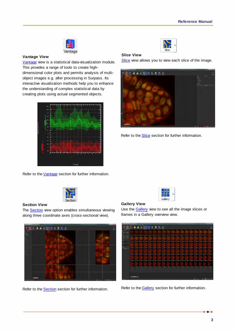
Vantage View

Vantage view is a statistical data-visualization module.

This provides a range of tools to create high-

dimensional color plots and permits analysis of multi-

object images e.g. after processing in Surpass. Its

interactive visualization methods help you to enhance

the understanding of complex statistical data by

creating plots using actual segmented objects.

Refer to the Vantage section for further information.

Slice View

Slice view allows you to view each slice of the image.

Refer to the Slice section for further information.

Section View

The Section view option enables simultaneous viewing

along three coordinate axes (cross-sectional view).

Refer to the Section section for further information.

Gallery View

Use the Gallery view to see all the image slices or

frames in a Gallery overview view.

Refer to the Gallery section for further information.

IMARIS

4

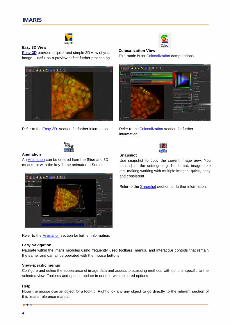
Easy 3D View

Easy 3D provides a quick and simple 3D view of your

image - useful as a preview before further processing.

Refer to the Easy 3D section for further information.

Colocalization View

This mode is for Colocalization computations.

Refer to the Colocalization section for further

information.

Animation

An Animation can be created from the Slice and 3D

modes, or with the key frame animator in Surpass.

Refer to the Animation section for further information.

Snapshot

Use snapshot to copy the current image view. You

can adjust the settings e.g. file format, image size

etc. making working with multiple images, quick, easy

and consistent.

Refer to the Snapshot section for further information.

Easy Navigation

Navigate within the Imaris modules using frequently used toolbars, menus, and interactive controls that remain

the same, and can all be operated with the mouse buttons.

View-specific menus

Configure and define the appearance of image data and access processing methods with options specific to the

selected view. Toolbars and options update in context with selected options.

Help

Hover the mouse over an object for a tool-tip. Right-click any any object to go directly to the relevant section of

this Imaris reference manual.

Reference Manual

5

1.1 Installation and License InformationImaris software is delivered on a standard CD or downloaded from www.bitplane.com. The CD includes a folder

containing the necessary manuals, or the manuals can be downloaded.

Imaris runs on:

MS Windows 10 x64

MS Windows 8 x64

MS Windows 7 x64

Mac OS X 10.9 to 10.13

Intel based MAC

Please note: Windows 8 and 10 do not come with the .net 3.5 and prior framework required for the

matlab runtime which Imaris XTensions use. In order to enable this ‘Windows Feature’ you will need

an administrator account. You can set this under Control Panel -> Programs and Features, left hand

side panel contains ‘Turn Windows features on or off’.

To find the latest information about minimum and recommended hardware requirements please visit our web

site - the Support section.

Installation

To install the software, please proceed as follows:

1. Insert your Imaris CD-Rom in the computer.

2. Follow the instructions on the screen.

3. The installation is completed automatically.

Licensing

To run Imaris, the appropriate licenses for the required modules, such as Imaris base, ImarisTime, ImarisColoc

or Imaris MeasurementPro. Without licenses, Imaris can only be run in a restricted mode. In case of any

license problems, please refer to the support information on our website www.bitplane.com for detailed

instructions.

Starting Imaris

Imaris can be started by one of the following methods:

Double-click on the Imaris icon (we recommend copying the icon to the desktop).

Drag the icon of an image or a file to the Imaris program icon.

The software opens with the main screen.

Supported File Formats

Imaris (as of version 5.5) can read the following file formats, i.e. it can read the image and the parameters.

Andor: Multi-TIFF series (*.tif, *.tiff)

Andor: MM (*.kinetic)

IMARIS

6

Andor: iQimage (*.kinetic)

Applied Precision, Inc: DeltaVision (*.r3d, *.dv)

Biorad: MRC-600, MRC-1024 (series)(*.pic)

BioVision: IPLab Mac (*.ipm)

Bitplane: Imaris 5.5 (*.ims)


Bitplane: Imaris 2.7 Classic/Old (*.ims)

Bitplane: Imaris Scene File (*.imx)

BMP (adjustable file series) (*.mrc, *.st, *.rec)

Carl Zeiss: LSM 510 (*.lsm)

Carl Zeiss: LSM 410, LSM 310 (*.tif, *.tiff)

Carl Zeiss: Axiovision (*.zvi)

Compix:Simple PCI (*.cdx)

Image Cytometry Standard: ICS - used by Nikon, Huygens, and others (*.ics, *.ids)

Gatan Digital Micrograph (serie):(*.dm3)

Leica: TCS-NT (*.tif, *.tiff)

Leica: LCS (*.lei, *.raw, *.tif, *.tiff)

Leica: series (*.inf, *.info, *.tif, *.tiff)

Leica: Image File Format (*.lif)

MetaSystem: Meta Viewer (*.imv)

Molecular Devices: Metamorph STK (series) (*.stk)

Molecular Devices: Metamorph ND (*.nd)

MRC: primarily electron density volumes as in cryo-EM (*.mrc, *.st, *.rec)

Nikon: ND2 (*.nd2)

Olympus: FluoViewTIFF (*.tif, *.tiff)

Olympus: 1000 OIF (*.oif)

Olympus: 1000 OIB (*.oib)

Olympus: Cell^R 1.1/standard (*.tif, *.tiff)

Olympus:Virtual Slide Image (*.vsi)

Opellab: liff (series) (*.liff)

Openlab: raw (*.raw)

Open Microscopy Environment XML (*.ome)

Open Microscopy Environment TIF (*.tif, *.tiff)

Perkin Elmer: UltraView (*.tim, *.zpo)

Prairie Technologies: Prairie (*.xml, *.cfg, *.tif, *.tiff)

Scanalytics: IPLab (*.ipl)

Slide Book (*.sld)

TIFF (adjustable file series) (*.tif, *.tiff)

TILL Photonics: TILLvisION (*.rbinf)

Imaris can also read general TIFF series (or BMP series) in the format aaaNNN.tif (where a is a character and N

is a number).

Reference Manual

7

1.2 About this manualInformation in this manual is subject to change without notice and does not represent a commitment on the part

of Bitplane AG. Bitplane AG is not liable for errors contained in this manual or for incidental or consequential

damages in connection with the use of this software.

This document contains proprietary information protected by copyright. No part of this document may be

reproduced, translated, or transmitted without the express written permission of Bitplane AG, Zurich,

Switzerland.

For further questions or suggestions please visit our web site at:

www.bitplane.com

or contact our support teams:

[email protected]

[email protected]

[email protected]

Bitplane AG

An Oxford Instruments Company

Badenerstrasse 682

8048 Zurich

Switzerland

© May 2018, Bitplane AG, Zurich.

All rights reserved. Printed in the UK.

Imaris Reference Manual developed to support Imaris release 9.2

http://www.bitplane.com

mailto:[email protected]



IMARIS

8

Section 2 Arena View

The Arena View provides an easy-to-use image management interface. Image analysis often requires the

application of the same creation parameters to any number of images. Arena lets you speed up this process by

enabling "batch processing" to be performed on multiple images.

The Arena is your central working area in Imaris and an interface for visualizing, processing, analyzing and

interpreting all your images. This is where you add images and creation parameters, create and execute batch

runs, and configure all your statistical data-visualization settings.

The Arena view consists of a number of elements.

The search field is at the top left of the Arena view. Below the search field is the Arena Tree. The Arena tree

allows easy access to all Arena items. On the left hand side of this view you will find the Arena tree which

allows navigation of the folder structure. The pane on the right hand side of the Arena view display contents of

the current tree location or any search results. When an item is selected further information about this object

will display showing the selected object’s Properties, tags and surpass objects where appropriate. The

rightmost three quarters of the Arena view display contents of the current tree location or any search results.

The lower section of the Arena view displays the Tags tab or the Properties area with additional information

about the currently selected image. At the bottom right hand side of the Arena view is Zoom.

In Arena view Zoom can be used to change how the images are displayed. You can select from: Details that

provides a summary of the image files, or Small, Medium or Large Icons, these are shown in order from left to

right below. Zoom can help you navigate and find the required image, if you have many, or similar stored

images.

Reference Manual

9

Above: From left to right - Details, Small Icon, Medium Icon, Large Icon

Arena Items

Each Arena item has a number of different properties associated with it. Properties information affects how

items are visualized or processed. Some properties are fixed and others are user-defined.

Every Arena item is represented and displayed as an icon with its name written underneath. The following table

presents each item along with its associated icon:

Arena item Icons

Assay Empty Filled

Group Empty Filled

Image

Creation parameters

Collection Batch Collection Manually created Collection

Vantage Plot

Depending on the selected item, a right-click displays different options. The type of item determines what

options and tools are available.

Using Imaris Without Arena

Imaris has been developed so that the Arena provides the most effective means of accessing and managing

your images, and image data. It is however also possible to configure Imaris (version 8.3.0 onwards) so that

Arena View is not used. During installation, an option is provided to not use Arena. Using Arena is

recommended- if you want to install Imaris without Arena, please contact Bitplane support for further

information.

IMARIS

10

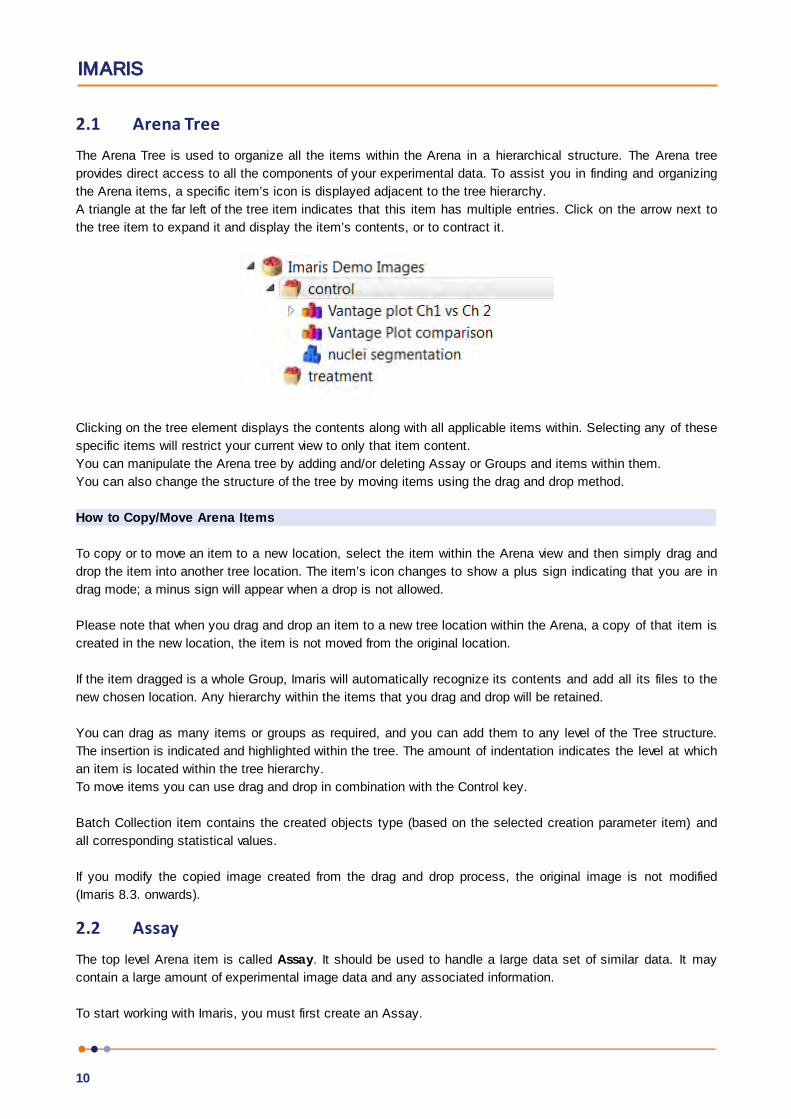
2.1 Arena TreeThe Arena Tree is used to organize all the items within the Arena in a hierarchical structure. The Arena tree

provides direct access to all the components of your experimental data. To assist you in finding and organizing

the Arena items, a specific item’s icon is displayed adjacent to the tree hierarchy.

A triangle at the far left of the tree item indicates that this item has multiple entries. Click on the arrow next to

the tree item to expand it and display the item’s contents, or to contract it.

Clicking on the tree element displays the contents along with all applicable items within. Selecting any of these

specific items will restrict your current view to only that item content.

You can manipulate the Arena tree by adding and/or deleting Assay or Groups and items within them.

You can also change the structure of the tree by moving items using the drag and drop method.

How to Copy/Move Arena Items

To copy or to move an item to a new location, select the item within the Arena view and then simply drag and

drop the item into another tree location. The item’s icon changes to show a plus sign indicating that you are in

drag mode; a minus sign will appear when a drop is not allowed.

Please note that when you drag and drop an item to a new tree location within the Arena, a copy of that item is

created in the new location, the item is not moved from the original location.

If the item dragged is a whole Group, Imaris will automatically recognize its contents and add all its files to the

new chosen location. Any hierarchy within the items that you drag and drop will be retained.

You can drag as many items or groups as required, and you can add them to any level of the Tree structure.

The insertion is indicated and highlighted within the tree. The amount of indentation indicates the level at which

an item is located within the tree hierarchy.

To move items you can use drag and drop in combination with the Control key.

Batch Collection item contains the created objects type (based on the selected creation parameter item) and

all corresponding statistical values.

If you modify the copied image created from the drag and drop process, the original image is not modified

(Imaris 8.3. onwards).

2.2 AssayThe top level Arena item is called Assay. It should be used to handle a large data set of similar data. It may

contain a large amount of experimental image data and any associated information.

To start working with Imaris, you must first create an Assay.

Reference Manual

11

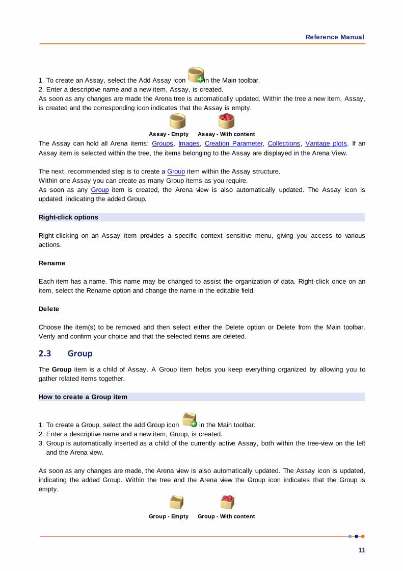
1. To create an Assay, select the Add Assay icon in the Main toolbar.

2. Enter a descriptive name and a new item, Assay, is created.

As soon as any changes are made the Arena tree is automatically updated. Within the tree a new item, Assay,

is created and the corresponding icon indicates that the Assay is empty.

Assay - Empty Assay - With content

The Assay can hold all Arena items: Groups, Images, Creation Parameter, Collections, Vantage plots. If an

Assay item is selected within the tree, the items belonging to the Assay are displayed in the Arena View.

The next, recommended step is to create a Group item within the Assay structure.

Within one Assay you can create as many Group items as you require.

As soon as any Group item is created, the Arena view is also automatically updated. The Assay icon is

updated, indicating the added Group.

Right-click options

Right-clicking on an Assay item provides a specific context sensitive menu, giving you access to various

actions.

Rename

Each item has a name. This name may be changed to assist the organization of data. Right-click once on an

item, select the Rename option and change the name in the editable field.

Delete

Choose the item(s) to be removed and then select either the Delete option or Delete from the Main toolbar.

Verify and confirm your choice and that the selected items are deleted.

2.3 GroupThe Group item is a child of Assay. A Group item helps you keep everything organized by allowing you to

gather related items together.

How to create a Group item

1. To create a Group, select the add Group icon in the Main toolbar.

2. Enter a descriptive name and a new item, Group, is created.

3. Group is automatically inserted as a child of the currently active Assay, both within the tree-view on the left

and the Arena view.

As soon as any changes are made, the Arena view is also automatically updated. The Assay icon is updated,

indicating the added Group. Within the tree and the Arena view the Group icon indicates that the Group is

empty.

Group - Empty Group - With content

IMARIS

12

A Group can contain 2D, 3D and 4D images or any other Arena item.

A typical Group consists of many images, creation parameters, Batch results, and/or Vantage plot items.

Within the Group, each Arena item is labeled with a special icon. The icon graphically indicates the type of

item.

The next step is to add Image items within the Group.

As soon as any item is added within the Group, the Arena view is also automatically updated. The Group icon

is updated, indicating that content has been added.

Right-click options

Right-clicking on a Group item provides a specific context sensitive menu offering you various actions.

Rename

Each item has a name. This name may be changed to assist organization of data. Right-click once on an item

and select the rename option and in an editable field change the name.

Delete

Select the item(s) to be removed and select the Delete option or Delete from the Main toolbar. Verify and

confirm your selection and the selected items are deleted.

Please note: Creating and using a Group is helpful if you want to experiment with a potential creation

parameters sets.

2.4 ImageA Group can contain 2D, 3D and 4D images. All images within Arena view are displayed as thumbnails.

How to add Image items

To add images within the Group select Image in the main toolbar then select the Add Image icon .

This opens a new window from which you can browse and select the required files. In the Open window, select

the files you want to add to the Group. Click on the desired file name or select multiple files using standard

multiple file selection commands.

How to add an Image Folder

To add image folders select Image in the main toolbar then select the Add Image Folder icon .

This opens a new window from which you can browse and select the required folder. In the Open window, select

the folder you want to add. This will add image files within the selected folder that are in the supported file

formats. To add images within subfolders click Recursively add subfolder. This will add images within

subfolders, keeping the file structure of the selected folder.

Once you have selected your image(s) and Imaris has finished adding the files, the image’s thumbnail appears

within the Arena view. Within the tree, the Group icon will change indicating that the Group is populated. Place

all relevant images for analysis in a single group.

Reference Manual

13

Imaris collects relevant information from supported file formats when they are added within the Arena and sets

the relevant metadata within the Properties Tab automatically.

You can place the same image file in as many groups as you like. To add an image file to another Group, either

repeat the same procedure or alternatively select the image thumbnail and drag and drop it into the required

Group.

A small icon in the bottom left corner of the image thumbnails indicates the image type and/or any created

objects. Each image may be viewed in a number of different ways. The way that you open the image depends

on the type of images and how you want to view and work with it.

The default view is to open the image with the created objects and batch results.

Right-click options

Image view may be adjusted to the most useful option by right-clicking. Depending on the selected image, the

right click opens a list that allows you to choose between different Surpass view visualization options. The

following options are available:

Open with objects and Batch results

Once the batch run is completed, to validate the Batch segmentation results you can open the image with all

created objects and batch results.

Open with objects from file only

This option opens image data and all previously created Surpass objects from the selected file.

Open with batch results

After the Batch run is completed, the batch segmented images can be compared with the original raw data to

make sure that no structure not seen in the original data has been introduced by batch processing.

Open image only

This option opens image data only.

Open image resampled

The Resampling Open dialog box can be used as a preview before loading the data set and allows you to

change the resolution of the data (subsampling) and to select only a part of the data set (cropping) by

specifying the parameters in the Resampling Open dialog box. Both options reduce the size of the data set,

decreasing the time needed to read the file and speeding up any operations on the data. This is particularly

helpful/beneficial when reading large data sets over a network.

2.4.1 Image Choice within the Group

If you require your images to be segmented and analyzed in a certain way in the batch run, make sure they are

selected in one Group.

IMARIS

14

Added images within one Group should be scientifically relevant and similar in any other quality attributes, as

may be scientifically relevant to the batch results. Due to the essence of batch processing, a well grouped

image is essential to ensure reliability between different batch results and ensures the comparability of the

different experimental groups.

You should make sure that you are working with a group of images acquired under largely uniform conditions.

Also always make sure you have selected all images within the Group that you want to appear in the Batch

Collection. Once the Batch job is completed you can modify the image selection within the Group. However,

please note that any modifications that you make to the image selection do not affect the previously created

Batch Collection item.

When the image files have been successfully added within the Group items, identify the most-representative

image of the whole group. The image will be used to define the Creation Parameters and the entire batch

settings.

To inspect the image, double-click on the thumbnail to open it in the Surpass view.

2.4.2 Open

Data sets can be loaded from various file formats.

Image File Series

If the data set consists of a series of images each is stored as an individual file. To open a series of images

select the folder and click on Open to open it.

This brings up the Image selection window, which allows you to explore your file system.

The window contains a preview of all the images as well as the following info: Name, Description, Recording

date, Size, Time Points, Channels, Total size and Voxel size.

The image series is ordered according to the number, which appears after the file name suffix.

To open the image select a file name from the list and click Open.

Image Preview

Check the box Thumbnail Preview to activate an image preview.

Search Image name

Enter the image name for instant image selection.

Resampling Open...






1. In the menu select File – Open.

2. Select a file name from the list and click Open or double-click on the requested file entry.

3. The file is loaded.

Imaris Background Load

If you need to open a large time series data set, Imaris Background Load feature loads the data in sequential

Reference Manual

15

time points according to the sort order and demonstrates an advantage in speed performance over the other

methods.

iQ files in Imaris

To open iQ files in Imaris:

1. Locate and select the DiskInfo5.kinetic file.

2. Click on the ‘Settings’ button to open a new window with a list of images and image information.

3. Check the box Thumbnail Preview to activate an image preview.

4. Select the required image and click on the OK button.

5. Then click again on the Open button. This will instantly create 3D volume rendered image of the selected

data set.

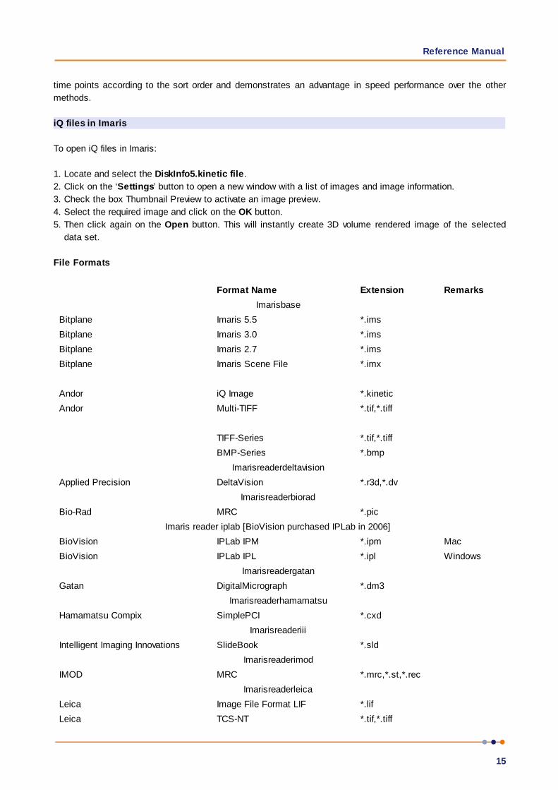
File Formats

Format Name Extension Remarks

Imarisbase

Bitplane Imaris 5.5 *.ims



Bitplane Imaris Scene File *.imx

Andor iQ Image *.kinetic

Andor Multi-TIFF *.tif,*.tiff

TIFF-Series *.tif,*.tiff

BMP-Series *.bmp

Imarisreaderdeltavision

Applied Precision DeltaVision *.r3d,*.dv

Imarisreaderbiorad

Bio-Rad MRC *.pic

Imaris reader iplab [BioVision purchased IPLab in 2006]

BioVision IPLab IPM *.ipm Mac

BioVision IPLab IPL *.ipl Windows

Imarisreadergatan

Gatan DigitalMicrograph *.dm3

Imarisreaderhamamatsu

Hamamatsu Compix SimplePCI *.cxd

Imarisreaderiii

Intelligent Imaging Innovations SlideBook *.sld

Imarisreaderimod

IMOD MRC *.mrc,*.st,*.rec

Imarisreaderleica

Leica Image File Format LIF *.lif

Leica TCS-NT *.tif,*.tiff

IMARIS

16

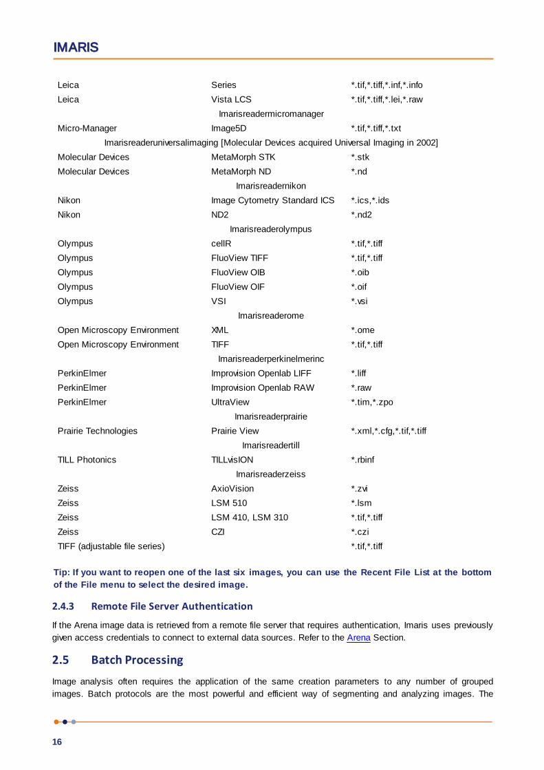
Leica Series *.tif,*.tiff,*.inf,*.info

Leica Vista LCS *.tif,*.tiff,*.lei,*.raw

Imarisreadermicromanager

Micro-Manager Image5D *.tif,*.tiff,*.txt

Imarisreaderuniversalimaging [Molecular Devices acquired Universal Imaging in 2002]

Molecular Devices MetaMorph STK *.stk

Molecular Devices MetaMorph ND *.nd

Imarisreadernikon

Nikon Image Cytometry Standard ICS *.ics,*.ids

Nikon ND2 *.nd2

Imarisreaderolympus

Olympus cellR *.tif,*.tiff

Olympus FluoView TIFF *.tif,*.tiff

Olympus FluoView OIB *.oib

Olympus FluoView OIF *.oif

Olympus VSI *.vsi

Imarisreaderome

Open Microscopy Environment XML *.ome

Open Microscopy Environment TIFF *.tif,*.tiff

Imarisreaderperkinelmerinc

PerkinElmer Improvision Openlab LIFF *.liff

PerkinElmer Improvision Openlab RAW *.raw

PerkinElmer UltraView *.tim,*.zpo

Imarisreaderprairie

Prairie Technologies Prairie View *.xml,*.cfg,*.tif,*.tiff

Imarisreadertill

TILL Photonics TILLvisION *.rbinf

Imarisreaderzeiss

Zeiss AxioVision *.zvi

Zeiss LSM 510 *.lsm

Zeiss LSM 410, LSM 310 *.tif,*.tiff

Zeiss CZI *.czi

TIFF (adjustable file series) *.tif,*.tiff

Tip: If you want to reopen one of the last six images, you can use the Recent File List at the bottom

of the File menu to select the desired image.

2.4.3 Remote File Server Authentication

If the Arena image data is retrieved from a remote file server that requires authentication, Imaris uses previously

given access credentials to connect to external data sources. Refer to the Arena Section.

2.5 Batch ProcessingImage analysis often requires the application of the same creation parameters to any number of grouped

images. Batch protocols are the most powerful and efficient way of segmenting and analyzing images. The

Reference Manual

17

ability of Imaris to batch process a group of images to produce a statistical data-visualization report is the

essence of Imaris Arena view.

Batch processing enables you to apply the same creation parameters to all images within the selected Group,

sparing you the repetitive work.

This section lists the components of the batch processing framework in Imaris and provides an overview of the

steps you have to follow to create a creation parameters item, a batch run and analyze the results of the batch.

Before you start analyzing your images there are some aspects to be confirmed and a few steps to be

completed before pressing "go" on any batch run.

The batch process has the following stages:

1. To apply the same creation parameters all images within the Group, first you need to set them up.

2. Storing these creation parameters generates a new Arena item, the Creation Parameters item

3. Then double check your image selection within the Group before selecting the Batch processing option.

4. Right-click on Creation parameter items and select the Run Batch job option.

The creation parameters are automatically applied to all images within the Group and simultaneously, a new

Arena item, the Batch Collection item is created.

5. Once the Batch job is completed you can analyze the results within Vantage view.

2.6 Creation ParametersTo be able to apply the creation parameters to all images within the Group you need to set them up.

Identify the most representative image of the whole group.

Double-click on the image thumbnail to open it in the Surpass view.

Complete an appropriate Creation Wizard (Cells, Filament, Spots and Surfaces) and create the required

objects.

Under the Creation Tab (Cells, Filament, Spots and Surfaces) all processing instructions and the parameter’s

value are listed. The Store Parameters for the Batch button allows you to save the complete set of the

creation parameters and all relevant settings.

In the Store Creation Parameter window, enter a descriptive name for your creation parameters and select the

Arena option as the required store location.

When you select the Arena option, a new item is automatically created within the Arena view. The Arena view

is updated, a new Creation Parameters item is displayed.

How to apply the same creation parameters in multiple Groups

As image analysis often requires the application of the same creation parameters to any number of grouped

images, the selected creation parameters item can be copied between the Group(s).

In addition to copying the selected creation parameters item, you can also import it into the newly chosenGroup. To do so, select the Group and click on the Creation button. The creation parameters file (*icpx) is

IMARIS

18

imported.

Please note that only creation parameters files (*icpx) generated by the Export command can be imported.

How to copy Creation Parameters item

To copy the creation parameters from one Group to a new one, select the creation parameters item that you

want to copy and then drag and drop it into the newly chosen Group.

Right-click options

Right-clicking on a Creation Parameter item provides a specific context sensitive menu offering you various

actions.

Run Batch Job

Before selecting the Run Batch job option double check your image selection within the Group.

As soon as you press the Run Batch Job option Imaris generates a new Arena item, the Batch Collection item

. To create a Batch Collection item, Imaris applies the selected creation parameters set, (that you created

for the chosen image) to all images within the Group. A Batch Collection item contains the image’s data and

batch segmented objects along with the related statistical calculation.

Run Batch including Sub-Groups

This option recursively applies the creation parameters to all the images of the chosen Assay/ Group and all its

subgroups.

As soon as you press the Run Batch Job option Imaris generates a new Arena item, the Batch Collection item

within the selected Assay/ Group and all its subgroups.

To create a Batch Collection item, Imaris applies the selected creation parameters set, (that you created for the

chosen image) to all images within the Group. A Batch Collection item contains the image’s data and batch

segmented objects along with the related statistical calculation.

Export

Select the creation parameters item you would like to export and click the Export button. If necessary, rename

and save the file in the chosen location. The Imaris creation parameters file will have an .icpx suffix.

Rename



Delete



Reference Manual

19

2.7 CreationIn addition to creating a new set of creation parameters you can also import a creation parameters file. By

clicking the Creation button, the creation parameters files (*icpx) generated by the Export command can be

imported into Imaris Arena or Surpass view.

Under the Edit/Preference/Creation Parameters the Export and Import buttons provide an easy way to

exchange creation parameters between different users or Arena groups.

2.8 Batch CollectionAs soon as you press the Run Batch Job option Imaris generates a new Arena item, the Batch Collection item

.

To create a Batch Collection item, Imaris applies the selected creation parameters, to all images within theGroup. Within the Group, each image is segmented and analyzed, the selected objects are created and thecorresponding statistical data is calculated. All this information is collected and stored within the BatchCollection item.

The Batch Job execution process and status are indicated by a set of overlaid icons placed in the bottom

corner of the Batch Collection item and the image thumbnail.

The following status icons are used:

1. Completed - the image is segmented and analyzed

2. Processing. The proportion of the complied Bath Job is indicated by an icon displaying

corresponding circle segments

3. Failed - the image(s) have not been segmented and analyzed

After the creation parameters have been successfully applied to an image, the icon in the bottom corner of the

image thumbnail shows that the batch job is completed .

The Batch Results Collection item appears in the Arena tree directly below the corresponding Group item.

Batch Collection Name

The Batch Collection is given a default name. This is the creation parameter file name with the Group name

prefix.

Once the Batch job is completed you can modify the image selection within the Group. However, please note

that any modifications that you make to the image selection do not affect the created Batch Collection.

Batch Collection item lets you retrieve segmented images quickly without affecting your original files. It also

allows you to copy the selected batch processed results into your Vantage plot item and then analyze them

further.

Right-click options

Right-clicking on a Batch Collection item provides a specific context sensitive menu offering you various

IMARIS

20

actions.

Create Vantage Plot

Vantage plots are the most informative and flexible way to visualize and generate a Batch Collection report.

Vantage Plot item provides a statistical data-visualization of the currently selected Batch Collection item.

Export Statistics

For some further statistical analysis you can export the data either as a Comma Separated Values file, or

directly as an Excel file. Imaris offers several data exporting options.

Click on the selected export button and select the file type.

All generated statistical data are exported to Excel, which starts automatically, and sorted in different sheets.

Rename



Delete



2.8.1 Batch Results Validation

After the batch run is completed, the batch segmented images can be compared with the original raw data to

make sure that no structure not seen in the original data has been introduced by batch processing.

Once the batch run is completed, to validate the Batch segmentation results you can open the image with the

default view Open with objects and Batch results or with a right-click on the image, then select the Open

with batch results option.

This option opens the image in the Surpass view.

Within the Surpass tree you will notice that the regular object icon has been changed. A new icon ,

superimposed on the object type icon, indicates that the required objects were batch created and therefore you

will not be able to manually modify them. Please note that these objects do not have an Edit tab. Under the

Creation tab, the Duplicate and Rebuild button provides two functions:

1. To copy the Batch created objects to a new Surpass Tree object.

2. To re-enter the Creation Wizard and use previous parameter settings and processing instructions as initial

values.

If you are not pleased with the Batch segmentation results and you find it necessary to manually modify them,

please remember that all the changes that you make will not be reflected in the Batch Collection item.

To modify the batched processed image you can open it and start a new creation wizard. As you proceed with

the new creation wizard, in each step, all creation parameters are initially set to match the batch creation

parameters’ values. Adjust them and modify all parameters as necessary to obtain new segmentation results.

These newly segmented objects must be saved using either the Store or Store as option. As Imaris does not

allow the modification of batch created objects, these newly segmented objects have the same characteristics

Reference Manual

21

as Manually created ones.

Once the manually created changes have been saved, within the Arena, the image thumbnail is updated. In its

corner, a small overlaying object icon appears and indicates that the created objects has been assigned to an

image.

To combine and compare these modified objects with the automatic Batch Results Collections, follow the

procedure described in the Manual Collection Section.

2.9 Batch QueueThe Batch Queue window displays the batch status. The batch queue table lists the current job(s) as well as a

list of all completed batch jobs.

For each job a short description is displayed: name, the current state of the job, the time at which the job has

been submitted and finished as well as the progress percentage.

A keyboard shortcut to open the Batch Queue window is Ctrl+Shift+B.

2.10 Manual CollectionSometimes you are confronted with a situation in which a few images that are not automatically well

segmented by the Batch creation parameters. In this case a manual object creation should be used for the

image segmentation.

The Manual Collection item allows you to combine for manually created objects with the automatic Batch

Collections within one Vantage Plot item. You can use a Manual Collection item to specify a data set that

contains manually created objects as an alternative input to the generate Vantage Plot comparison items.

To create a Manual Collection item select the Collection icon on the Main toolbar and a new Arena item

is created. Within the Arena tree, the Manual Collection item is created.

A small icon in the bottom left corner of the item indicates that contains manually created Surpass objects

.

Within the Surpass view, the manually created objects are not automatically stored and therefore your image

changes will not be automatically updated within the Arena. Therefore, please store the image after finishing

with a manual object creation. All manually created objects should be stored either by using the Store or

Stored as option. Once stored, they will appear in the Arena view. This newly created image item has an

overlaid icon indicating the image type and segmented surpass objects. Under the Surpass Objects tab the

newly created object is added.

How to integrate the manually created Surpass objects into the Collection item

In the Arena, under the Surpass Objects option lists all created and stored object types. To assist you in

finding and organizing the created objects, each one is labeled with an object icon.

To integrate manually created objects within the Manual Collection item, select the object icon from the

Objects tab, then drag and drop it onto the chosen Manual Collection item.

As soon as you have drag and dropped the manually created objects within the Manual Collection item, a new

overlaid icon appears and showing the object type.

Right-click options

Right-clicking on a Batch Collection item provides a specific context sensitive menu offering you various

actions.

IMARIS

22

Create Vantage Plot

Vantage plots are the most informative and flexible way to visualize and generate a Collection report. Vantage

Plot item provides a statistical data-visualization of the currently selected Collection data.

Rename

Each item has a name. This name may be changed to assist organization of data. Right-click once on an item,

and then select the rename option and in an editable field change the name.

Delete



2.11 Vantage plotVantage plots are the most informative and flexible way to visualize and generate a batch report. It provides a

statistical data-visualization of the currently selected collection(s) of Batch Collection data. It facilitates the

analysis of the collection results and illustrates patterns and trends that are not immediately apparent by just

looking at the raw or segmented data.

Within the Vantage view there are many different plot types and a selection of various plot dimensions are

available so you can easily configure the appearance of the results..

There are two methods to create a Vantage plot item.

1. To visualize the Batch created objects, right-click on the Collection / Manual Collection item and

choose the Create Vantage plot option.

2. To create a Vantage Plot item, select the add Vantage icon in the Main toolbar. Enter a descriptive

name and a new item, Vantage Plot, is created. Vantage Plot is automatically inserted as a child of the

currently active Assay/ Group, both within the tree-view on the left and within the Arena view.

A Vantage Plot item provides the benefits of comparing Collection results of multiple groups.

Right-click on the Collection item or double-click on the Vantage plot items to open the Vantage view.

Right-click options

Right-clicking on a Vantage plot item provides a specific context sensitive menu offering you various actions.

Open in Vantage

Select this option to visualize the selected Batch Collection created objects within the Vantage view.

Rename

Each item has a name. This name may be changed to assist organization of data. Right-click once on an item,

Reference Manual

23

and then select the rename option and in an editable field change the name.

Delete



2.11.1 Comparison of multiple Groups’ Collections

A Vantage Plot item generates a separate plot component on a per group basis and allows you to visualize and

analyze Batch Collection results in a way that is meaningful and not overwhelming.

It helps you find relationships among several statistical variables, determine their relative importance and

therefore draw a comparison between Batch Collection results more clearly.

How to compare Batch Collection results

To see if two or more image Groups have scientifically relevant differences between them and assess the

degree of variation from one group to the next, create a Vantage plot item.

To create a Vantage plot item, select the add Vantage icon in the Main toolbar. Enter a descriptive name

and a new Vantage Plot item is created.

Then simply drag and drop the chosen Collection items from the selected Groups into the Vantage Plot

item .

To create the Vantage plot either right click on the Vantage Plot item and select the Open in Vantage option or

simply double-click on the Vantage Plot item.

Within the Vantage view, the comparison Vantage plot shows an arrangement of Batch Collections results

combined in one plot.

The Batch Collection results are overlaid, which helps you to determine how 'different' these image groups are.

Comparisons can be drawn between any selected statistical variables that you are interested in.

Within one Vantage Plot item you can drag and drop as many Batch Collection items as you wish to compare.

2.11.2 Arena Vantage view

In Vantage view, in the Plot Input area, a Vantage tree displays all source objects. In the Vantage Properties

Area you can choose the plot type and which variables are to be assigned to (X, Y, Z, Colour or scale) plot

dimensions. For more information on Vantage view and instructions on how to select a plot type and assign plot

dimensions, please refer to the Vantage view Section.

Store

Selecting the Store option stores the Vantage plot data and created Vantage plot item within the selected

Arena Group. Within the Arena tree, a subgroup Vantage appears (within the tree) and is named accordingly.

Selecting the Store option leads a dialog to appear prompting you for a descriptive name for the item.

In the Name field enter a descriptive name for your Vantage Plot item and click the OK button. This is the name

that will appear within the Arena view. Within the Arena tree, at the bottom of the selected group the newly

created Vantage plot item will appear.

IMARIS

24

Store as

Selecting the Store as option allows you to modify the already created Vantage plot item and creates a new

Vantage plot item within the selected Arena Group.

2.12 Properties TabThe Properties tab contains all image-related metadata.

2.13 Tags TabAdditional experiment or image data plays an essential part in the interpretation, querying and analysis of

images. There are many different types of data that may be associated with an image such as sample

preparation, experimental conditions or imaging parameters.

To store these types of additional information, the tagging field is available.

Under the Tabs tab, the Add Tag button allows further information to be entered about the selected item(s).

Text and description entered in the tag fields are searchable and may be used to store information about the

used creation parameters, the type of the Vantage plots or any other additional information.

The tag has no effect on item properties and it may be used anywhere within the Arena view to provide

additional information.

You can add Tagged Names and/or Description to one or more items.

Select the item(s) from the Arena view and dialog choose the Add tag option.

Add Tag

The Tagged dialog is displayed, which enables you to enter a Name and Value for the tag.

Delete Tag

To delete this property you must select the item, go to the Tagged Values tab and manually delete the item.

2.14 Objects TabThe Objects lists all manually created and stored object types.

To assist you in finding and organizing the created objects, each one is labeled with an object icon.

To integrate surpass objects within the Manual Collection item, select the object icon then drag and drop it onto

the chosen Manual Collection item.

The Manual Collection item allows you to combine for manually created Surpass objects with the automatic

Batch Collections within one Vantage plot item.

2.15 Tag SearchThe search field allows efficient interactive exploration of items to find a specific item and/or rapid scanning of

item tags or labels. It enables you to quickly locate any items within Arena.

In the search field enter your search criteria, an item’s tag, label, or description, and click on the Find icon

to display the search results. The search field provides you with a text and a description based search.

The Arena window displays the results, a set of items that match the entered search query. There are two ways

the search results can be displayed. You can choose to view them within all Arena items, or within the selected

Reference Manual

25

Group. To adjust the search results display, select the appropriate button.

Arena button

Selecting this option displays all results that meet the entered search term within the whole Arena view.

Selected Group (Group name is displayed)

Selecting this option displays results that meet the entered search term within the selected Group.

IMARIS

26

Section 3 Surpass View

The Surpass view provides extended functions for visualization, including:

A large viewing area with numerous tools for data preparation, presentation and manipulation.

A selection of different types of data display as well as any combination of them.

The possibility of loading additional External objects for comparison.

Surpass Grouping functions.

How to Open the Surpass View?

Click on the icon in the Main toolbar.

Select View - 3D View.

Press the key combination Ctrl + 5.

Save and Load Surpass Configuration

The actual Imaris configuration (including Surpass Tree and all existing Items) in the Surpass view is called

Scene and can be stored in a Scene file with the extension *.imx. The Scene can be loaded again to the same

data set or to another data set. For details please refer to Section Surpass View - Overview - Scene File

Concept.

See also:

3D View - Ortho Slice

3D View - Cells

3D View - Clipping Plane

3D View - Filament

3D View - Reference Frame

3D View - Frame

3D View - Surpass Group

3D View - Measurement Point

3D View - Oblique Slicer

3D View - Ortho Slicer

3D View - Light Source

3D View - Volume

3D View - Surfaces

3D View - Spots

3.1 Surpass ToolbarThe Surpass main toolbar provides quick access to frequently used items:

Arena

Vantage

Store

Store as

Export

Slice

3D View

Coloc

Annotate

Reference Manual

27

Animation

Snapshot

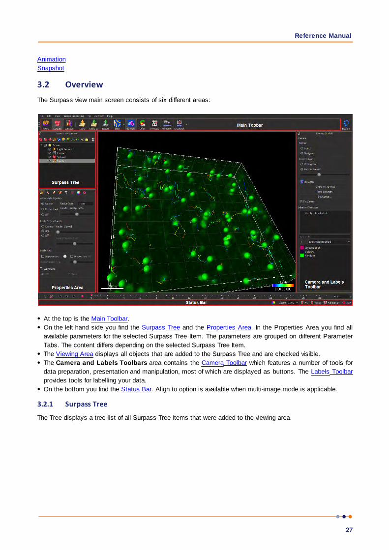
3.2 OverviewThe Surpass view main screen consists of six different areas:

At the top is the Main Toolbar.

On the left hand side you find the Surpass Tree and the Properties Area. In the Properties Area you find all

available parameters for the selected Surpass Tree Item. The parameters are grouped on different Parameter

Tabs. The content differs depending on the selected Surpass Tree Item.

The Viewing Area displays all objects that are added to the Surpass Tree and are checked visible.

The Camera and Labels Toolbars area contains the Camera Toolbar which features a number of tools for

data preparation, presentation and manipulation, most of which are displayed as buttons. The Labels Toolbar

provides tools for labelling your data.

On the bottom you find the Status Bar. Align to option is available when multi-image mode is applicable.

3.2.1 Surpass Tree

The Tree displays a tree list of all Surpass Tree Items that were added to the viewing area.

IMARIS

28

Structure

The tree list is automatically generated and updated when a Surpass Tree Item is added or deleted. The first

added object generates a Surpass Group - Scene. All following new objects are stored in this Surpass

Group. A name is generated automatically for each Surpass Tree Item. To change the name, double-click on

the item and enter a new name. Move objects or Surpass Groups from one to another by dragging and dropping

them with the left mouse button.

How to Add a new Surpass Tree Item?

All available Surpass Tree Items are available in the menu Surpass. To add new Surpass tree item click on the

icon.

You find a list of all Items in the Section Surpass View - Overview - Properties Area.

Display

Each Surpass Tree Item includes a check-box. Check the box to make the object visible in the viewing area.

Uncheck the box to make the object invisible in the viewing area. The currently active object in the viewing area

is highlighted in the Surpass Tree.

Surpass Groups

You can group objects into so-called component groups. Functions applied to the component group apply to all

of its members. This facilitates the application of colors or the deletion of objects.

Please note: If Group folder is checked invisible, all Items in the folder are invisible.

Multiple Selection

You may select more than one listed Item at a time for an operation. The selection functions in Surpass

correspond to the Windows functions:

Reference Manual

29

Consecutive: Press and hold the Shift-key down and select the first, then the last entry to be selected from

the list. All entries in between the two are also selected.

Selective: Press and hold the Ctrl-key down and select any required entries from the list.

All selected entries are highlighted and commands or operations apply to all of them.

Objects Toolbar

In the Objects toolbar you find a selection of Surpass Tree Items. To customize the Objects toolbar please refer

to Section Menu Edit - Preferences... - 3D View (Object Creation Buttons).

Button Delete...

To delete Surpass Tree Item, highlight the Item in the Surpass Tree and click the button Delete... . The Delete

selection window with a confirmation question is displayed.

Naming Conventions

Objects are automatically named by Surpass as follows:

Cells Cells n

Clipping Plane Clipping Plane n

Contour Surface Surface

External Object External Object n

Filament Filament n

Reference Frame Reference Frame n

Frame Frame

Surpass Group Surpass Group n

Surfaces Surface n

Light Source Light Source n

Measurement Point Measurement Points n

Oblique Slicer Oblique Slicer

Ortho Slicer Ortho Slicer n

Spots Spots n

Volume Volume (only one volume can be created)

Surpass Tree Item Properties

Each Surpass Tree Item has its own set of adjustable parameters. They are displayed in the properties area.

Surpass Tree Item Tabs

Each Surpass Tree Item has its own set of adjustable parameters. They are grouped in different Tabs.

Save and Load Surpass Tree Configuration

The actual Imaris configuration (including Surpass Tree and all existing items) in the Surpass view is called

Scene and can be stored in a scene file with the extension *.imx. The Scene can be loaded again to the same

IMARIS

30

data set or to another data set. For details please refer to Section Surpass View - Overview - Scene File

Concept.

See also:Menu Edit - Preferences... - 3D View (Object Creation Buttons)Menu Surpass - Delete Selected Objects... Surpass View - Overview - Properties AreaSurpass View - Surpass Group

3.2.2 Scene File Concept

The actual Imaris configuration (including Surpass Tree and all existing Items) in the Surpass view is called

Scene and can be stored in a scene file with the extension *.imx. The Scene can be loaded again to the same

data set or to another data set.

Surpass View - Surpass Group

3.2.3 Properties Area

The Properties Area displays all available parameters for the selected Surpass Tree Item.

Surpass Tree Item - Properties

The name of the heading is a combination of the selected Surpass Tree Item, followed by "- Properties". If you

select another Surpass Tree Item the heading changes accordingly.

Tab X

The parameters are grouped on different Parameter Tabs. The content differs depending on the selected

Surpass Tree Item.

List of available Tabs:

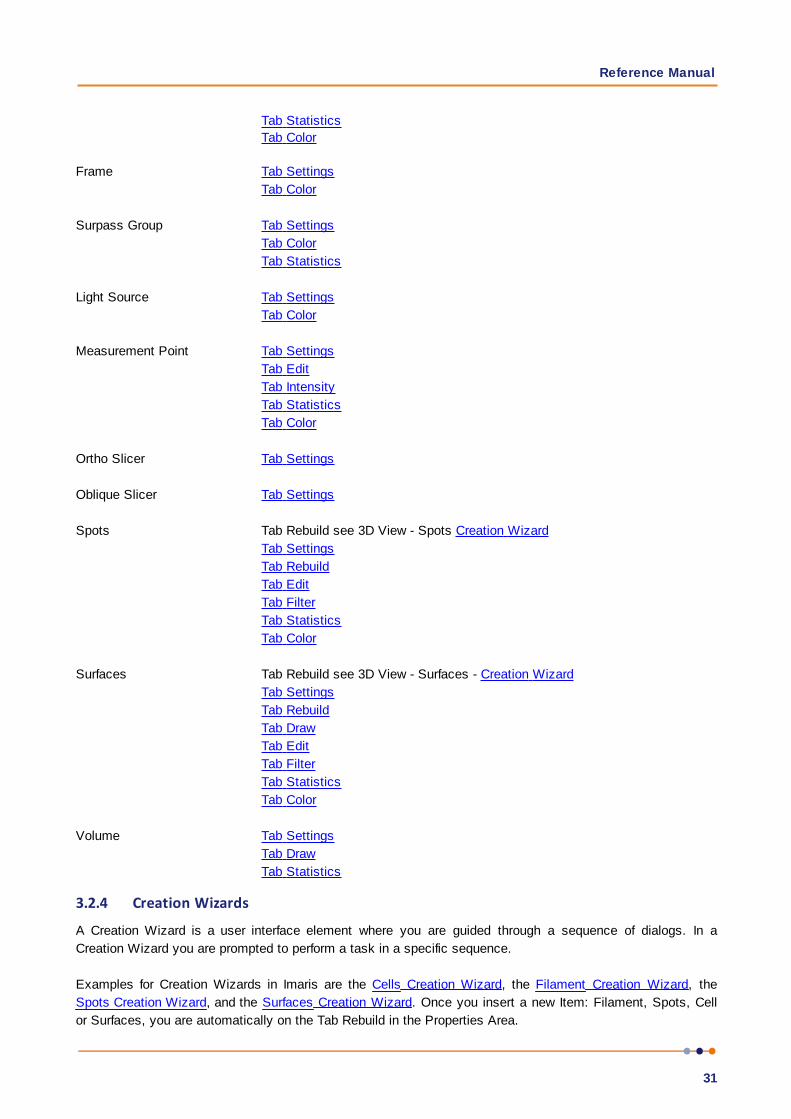
Surpass Tree Item Parameter Tab

Cells Tab Rebuild see 3D View - Cells Creation Wizard

Tab Settings

Tab Rebuild

Tab Edit

Tab Filter

Tab Statistics

Tab Color

Clipping Plane Tab Settings

External Object Tab Settings

Tab Color

Filament Tab Rebuild see 3D View - Filament Creation Wizard

Tab Settings

Tab Rebuild

Tab Draw

Tab Edit

Tab Filter

Reference Manual

31

Tab Statistics

Tab Color

Frame Tab Settings

Tab Color

Surpass Group Tab Settings

Tab Color

Tab Statistics

Light Source Tab Settings

Tab Color

Measurement Point Tab Settings

Tab Edit

Tab Intensity

Tab Statistics

Tab Color

Ortho Slicer Tab Settings

Oblique Slicer Tab Settings

Spots Tab Rebuild see 3D View - Spots Creation Wizard

Tab Settings

Tab Rebuild

Tab Edit

Tab Filter

Tab Statistics

Tab Color

Surfaces Tab Rebuild see 3D View - Surfaces - Creation Wizard

Tab Settings

Tab Rebuild

Tab Draw

Tab Edit

Tab Filter

Tab Statistics

Tab Color

Volume Tab Settings

Tab Draw

Tab Statistics

3.2.4 Creation Wizards

A Creation Wizard is a user interface element where you are guided through a sequence of dialogs. In a

Creation Wizard you are prompted to perform a task in a specific sequence.

Examples for Creation Wizards in Imaris are the Cells Creation Wizard, the Filament Creation Wizard, the

Spots Creation Wizard, and the Surfaces Creation Wizard. Once you insert a new Item: Filament, Spots, Cell

or Surfaces, you are automatically on the Tab Rebuild in the Properties Area.

IMARIS

32

See also:3D View - Cells - Creation Wizard

3D View - Filament - Creation Wizard

3D View - Spots - Creation Wizard

3D View - Surfaces - Creation Wizard

3.2.5 Viewing Area

Pan

To move the image within the Surpass view (pan the object) choose the mouse pointer mode Navigate. Click

and hold the right mouse button while dragging the mouse. Release right mouse button to place the image.

On a PC or with a three-button mouse or on a Mac:

Right-click & drag Pan image

On a Mac with a one-button mouse:

ctrl + click & drag Pan image

Rotate

Rotating an image allows to change the viewing angle on a three-dimensional object.

Choose the mouse pointer mode Navigate. Click with the left mouse button in the image and hold the button

down while moving the mouse (hold left + drag). The image on screen is rotated towards the direction the

mouse is dragged. Be sure to hold the left mouse button down during the whole rotation. Stop moving the

mouse and release the left mouse button to stop the rotation.


Left-click & drag Rotate image


Click & drag Rotate image

How to Keep the Image Continuously Rotated

Choose the mouse pointer mode Navigate. Click with the left mouse button in the image and hold the button

down while you move the mouse (hold left + drag). The image on screen is rotated towards the direction the

mouse is dragged. Release the left mouse button while still dragging the mouse. The result is a continued

rotation (speed of the rotation according to prior mouse motion). To stop the continued rotation re-click in the

image area.

Zoom

In the Surpass view you zoom the image either by using the mouse or by selecting one of the buttons in the

Status Bar at the bottom of the screen.

Reference Manual

33

Using the Mouse

Choose the mouse pointer mode Navigate. To zoom in on the image hold the middle mouse button and drag it

towards you. To zoom out from the image hold the middle mouse button and drag it away from you.


Middle-click & drag Move up: zoom out

Move down: zoom in


Shift + ctrl + click & drag Move up: zoom out

Move down: zoom in

Using the Buttons in the Status Bar

Zoom %

Imaris lets you enlarge or reduce the viewing size of your data set as is required with the Zoom function. You

can zoom from 10% to 1000%. To go to a predefined zoom level, click the percentage of enlargement or

reduction you want. To specify a custom level, just type a zoom value. At 100% zoom factor one pixel on

screen represents one voxel.

Button Fit

Click on this button to pan the position to best fit in the window and adjust the zoom factor.

Button Reset

Click on this button to reset the image to the original position, center the image in the middle and set the

optimal zoom factor.

Button Full Screen

Click on this button to maximize the viewing area to full size of the monitor. To return to the standard window

re-click on the button Full Screen in the lower right corner.

Viewing options for Zoom and rotate can be adjusted in Preferences for 3D View - please refer to 3D View

Preferences.

See also:

View

Toolbars - Status Bar

Surpass View - Overview - Camera Toolbar (Pointer Navigate)

IMARIS

34

3.2.6 Camera Toolbar

The toolbar to the right hand side provides the controls for the Camera and the Labels functions. Labels

functions are outlined in the Labels section.

Camera Pointer

Select

The cursor becomes an arrow. You use the pointer mode Select whenever you want to mark something in the

image, e.g. to set some Measurement Points on the object surface.

Navigate

The cursor becomes two rotating arrows. You use the pointer mode Navigate to move, rotate or zoom the image

in the viewing area.

Tip: You can easily switch between the two pointer modes using the ESC-key. The effect is directly

visible on screen by the altered mouse pointer display.

Camera Type

Orthogonal

Orthogonal display using parallel lines.

Perspective X

Perspective projection is a type of drawing, or rendering, that graphically approximates on a planar (two-

dimensional) surface. If you select Perspective the slider (see below) is active.

Slider X

If you select as camera type Perspective X (see above) the slider is active. Drag the slider to adjust the vertical

aperture angle of the camera.

InMotion is described in the section InMotion

Button Center to Selection

Click on the button Center to Selection to move the selection in the center of the viewing area.

Button Set Center...

Use this button to select a new center of rotation. Click on the button Set Center... and then onto the Scene to

define the new center on which the camera zooms in.

Please note: Rotation centers can be set on Surfaces, Contour Surface, Ortho Slicer and External

objects Additional drawing and stereo view options may be enabled- please refer to 3D View

Fix Center

Click the Fix Center checkbox to set the center of the 3D cursor position so it will rotate about this point even it

the image object is moved within the image viewing window.

Note: You can press the shortcut key F6 when the 3D cursor is visible to perform this function (the Fix

Center option in the Camera panel gets checked). This shortcut key will have no effect when the 3D

cursor is not visible.

Reference Manual

35

Draw Style (Enable Draw Style Settings enabled)

Select the draw style of the object from the drop-down list.

Full Featured

Shows all objects as they are.

Wireframe

Show the objects as a simple wireframe only.

Please note that this will only show the points and edges of the object, without hidden triangle surfaces.

Draws objects; Surfaces, Spots, Filaments, Cells and Measurement Points as red colored wireframe models.

Hidden Lines

Draws objects as wireframe models and hides all background lines.

Please note: Set Volume and OrthoSlicer objects invisible before selecting Hidden Lines.

No Texture

Draws objects without textures.

Bounding Box

Shows only the boxes surrounding the objects.

Wireframe Overlay

Lays a red wireframe model over objects; Surfaces, Spots, Filaments, Cells and Measurement Points.

Points

Draws objects as a point model.

Stereo (Enable Stereo Camera Settings enabled)

Off

No stereo display in the viewing area.

Red/Cyan Anaglyph

This display mode requires colored glasses.

Quad Buffer

This display mode requires shutter glasses.

Interleaved Rows

This display mode requires a screen with a lenticular plastic sheet, that overlays the image. The sheet is

molded to have the form of dozens of tiny lenses or prisms per inch.

Interleaved Columns

This display mode requires a screen with a lenticular plastic sheet, that overlays the image. The sheet is

molded to have the form of dozens of tiny lenses or prisms per inch.

Offset

Display of the offset (0...5).

IMARIS

36

Slider

Adjust the offset to get an optimized 3D effect. Use a small offset if you are far away from the screen, use a big

offset, if you are close to the screen. Click on the slider handle and move it to the desired position.

3.2.7 Labels Toolbar

The labels toolbar can be used to label various objects or tracks manually, or according to the filter options

available for the data type. Labels provide a useful way to tag and identify a subset of objects (or tracks) for

further analysis. The label or label group name (including partial string) may also be used in the Imaris search

(refer to Tag Search) to quickly locate any data sets which use that label.

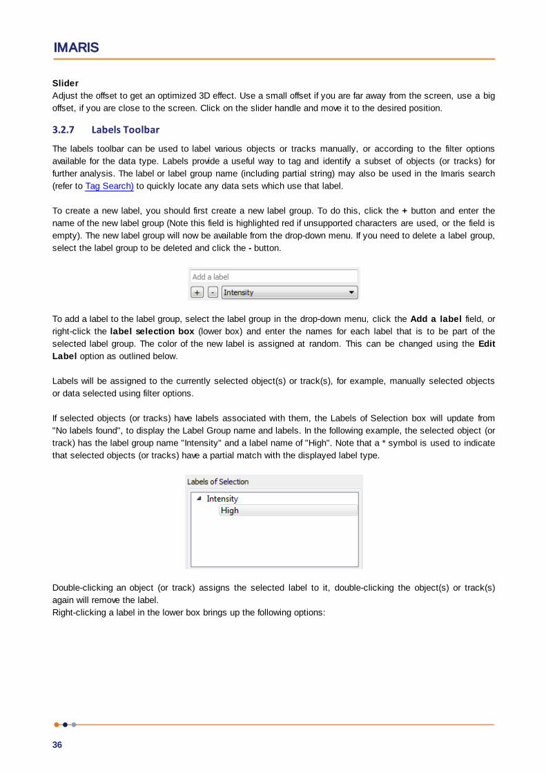
To create a new label, you should first create a new label group. To do this, click the + button and enter the

name of the new label group (Note this field is highlighted red if unsupported characters are used, or the field is

empty). The new label group will now be available from the drop-down menu. If you need to delete a label group,

select the label group to be deleted and click the - button.

To add a label to the label group, select the label group in the drop-down menu, click the Add a label field, or

right-click the label selection box (lower box) and enter the names for each label that is to be part of the

selected label group. The color of the new label is assigned at random. This can be changed using the Edit

Label option as outlined below.

Labels will be assigned to the currently selected object(s) or track(s), for example, manually selected objects

or data selected using filter options.

If selected objects (or tracks) have labels associated with them, the Labels of Selection box will update from

"No labels found", to display the Label Group name and labels. In the following example, the selected object (or

track) has the label group name "Intensity" and a label name of "High". Note that a * symbol is used to indicate

that selected objects (or tracks) have a partial match with the displayed label type.

Double-clicking an object (or track) assigns the selected label to it, double-clicking the object(s) or track(s)

again will remove the label.

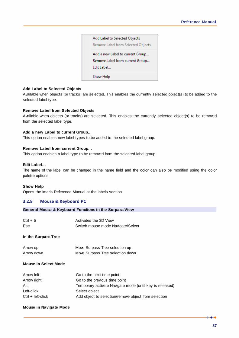
Right-clicking a label in the lower box brings up the following options:

Reference Manual

37

Add Label to Selected Objects

Available when objects (or tracks) are selected. This enables the currently selected object(s) to be added to the

selected label type.

Remove Label from Selected Objects

Available when objects (or tracks) are selected. This enables the currently selected object(s) to be removed

from the selected label type.

Add a new Label to current Group...

This option enables new label types to be added to the selected label group.

Remove Label from current Group...

This option enables a label type to be removed from the selected label group.

Edit Label...

The name of the label can be changed in the name field and the color can also be modified using the color

palette options.

Show Help

Opens the Imaris Reference Manual at the labels section.

3.2.8 Mouse & Keyboard PC

General Mouse & Keyboard Functions in the Surpass View

Ctrl + 5 Activates the 3D View

Esc Switch mouse mode Navigate/Select

In the Surpass Tree

Arrow up Move Surpass Tree selection up

Arrow down Move Surpass Tree selection down

Mouse in Select Mode

Arrow left Go to the next time point

Arrow right Go to the previous time point

Alt Temporary activate Navigate mode (until key is released)

Left-click Select object

Ctrl + left-click Add object to selection/remove object from selection

Mouse in Navigate Mode

IMARIS

38

S Set center (on Surfaces, Contour Surface, Ortho Slicer and External objects)



Left-click & drag Rotate image (scene)



Move down: zoom in

Shift + right-click & drag Move up: zoom out

Move down: zoom in

See also:

Addendum - Mouse & Keyboard PC

3.2.9 Mouse & Keyboard Mac

General Mouse & Keyboard Functions in the Surpass View

Command + 5 Activates the 3D View

Esc Switch mouse mode Navigate/Select

In the Surpass Tree

Arrow up Move Surpass Tree selection up

Arrow down Move Surpass Tree selection down

Mouse in Select Mode



Click Select object

Command-click Add object to selection/remove object from selection

Mouse in Navigate Mode

S Set center (on Surfaces, Contour Surface, Ortho Slices and External

objects)



With a one-button mouse:

Shift + ctrl + click & drag Move up: zoom out

Move down: zoom in

ctrl + click & drag Pan image


With a three-button mouse:

To configure a three button mouse on a Mac do the following:

Open the Apple-menu, select System Preferences... .

Reference Manual

39

Click on the button Keyboard & Mouse.

Select the OS X mouse properties.

Change the middle button to "Button 3".

Please note: Combined mouse buttons (e.g. left + middle mouse button) do not work in Imaris.


Move down: zoom in



See also:

Addendum - Mouse & Keyboard Mac

IMARIS

40

Section 4 Vantage View

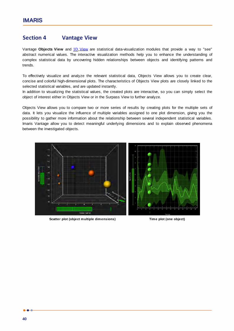
Vantage Objects View and 1D View are statistical data-visualization modules that provide a way to "see"

abstract numerical values. The interactive visualization methods help you to enhance the understanding of

complex statistical data by uncovering hidden relationships between objects and identifying patterns and

trends.

To effectively visualize and analyze the relevant statistical data, Objects View allows you to create clear,

concise and colorful high-dimensional plots. The characteristics of Objects View plots are closely linked to the

selected statistical variables, and are updated instantly.

In addition to visualizing the statistical values, the created plots are interactive, so you can simply select the

object of interest either in Objects View or in the Surpass View to further analyze.

Objects View allows you to compare two or more series of results by creating plots for the multiple sets of

data. It lets you visualize the influence of multiple variables assigned to one plot dimension, giving you the

possibility to gather more information about the relationship between several independent statistical variables.

Imaris Vantage allow you to detect meaningful underlying dimensions and to explain observed phenomena

between the investigated objects.

Scatter plot (object multiple dimensions) Time plot (one object)

Reference Manual

41

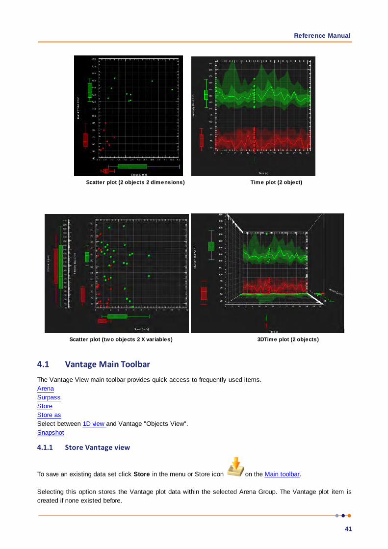
Scatter plot (2 objects 2 dimensions) Time plot (2 object)

Scatter plot (two objects 2 X variables) 3DTime plot (2 objects)

4.1 Vantage Main ToolbarThe Vantage View main toolbar provides quick access to frequently used items.

Arena

Surpass

Store

Store as

Select between 1D view and Vantage "Objects View".

Snapshot

4.1.1 Store Vantage view

To save an existing data set click Store in the menu or Store icon on the Main toolbar.

Selecting this option stores the Vantage plot data within the selected Arena Group. The Vantage plot item is

created if none existed before.

IMARIS

42

Please note: Store functionality is implemented to be performed at maximum speed. This functionality

overwrites the existing file without warning and only writes changed or new data without deleting obsolete ones.

As a result, the resulting Save file could actually be larger than the original.

4.1.2 Store as Vantage View

To store the changes made to the Vantage plot in a different Vantage plot item whilst maintaining the original

plot click on the Store as option or Store as icon .

This option enables you to modify the Vantage plot and its name and creates a new Vantage plot item within

the Arena view.

Enter the name for the file to be saved or confirm the suggestion.

Select the requested file format and click OK.

4.2 Vantage MenuPlease refer to the following sections:

Store

Store as

View

Vantage Plot

Preferences...

Help

4.2.1 Vantage Plot

Vantage Plot

To insert a new Vantage Objects View plot, click the Objects View icon.

Delete Selected Objects...

Select this option and in the Vantage Tree all highlighted items will be deleted.

Plot Numbers Area

Check the box Plot Numbers Area to display the tables that contains all statistical values used for the plot

creation.

4.3 Vantage User InterfaceThis Section describes the Vantage user interface for Objects View, and its various components.

Vantage Objects View consists of five working areas: Plot Tool Bar, Plot Input Data Area, Plot Property Area,

Plot Display Area and Plot Numbers Area.

Reference Manual

43

Follow these steps to start Imaris Vantage:

1. Create object(s) in the Surpass tree.

2. In the Toolbars, click on the Imaris Vantage icon.

3. Imaris Vantage is instantly started.

4. Imaris automatically creates a Vantage plot at the beginning of a Vantage session.

4.3.1 Plot Tool Bar

Use the Plot Tool Bar to add or remove plots from Vantage Object View.

The Plot Tool Bar contains two icons:

Imaris Vantage Delete

To create a new plot click on the Imaris Vantage icon and follow the Plot Creation Wizard.

Click an Imaris Vantage icon to instantly generate a new entry in the Plot Input Data Area.

To remove plots from Imaris Vantage click on the delete icon.

4.3.2 Plot Input Data Area

The Plot Input Data Area in Objects View displays a tree-like list of all created Vantage plots.

Each Vantage plot is organized in a tree-structured hierarchy. At the top of the hierarchy is the Vantage plot

and all source objects are listed below.

IMARIS

44

If in the first step of Plot Creation Wizard the selection of a source object changes, the tree is interactively

updated.

Vantage plot symbol reflects the type of the selected source object type. Each element of a Vantage Plot tree

has a check-box. Selecting or de-selecting the box next to the plot/object name controls its visibility in the Plot

Main Display Area.

The currently active plot/object is selected and highlighted. A set of its adjustable parameters is displayed in

Plot Property Area. The selection of the adjustable properties differs depending on the selected tree item;

Vantage plot or source object.

For a source object, only tabs that control how objects are individually displayed are available. These are:

Settings and Color.

For a Vantage Plot the following tabs are available: Settings, Creation, View, Edit, Frame and Color.

Changing properties for a Vantage Plot, changes also the corresponding properties for all objects in the tree.

To add a new Imaris Vantage plot click on the Imaris Vantage icon within the Plot Tool Bar. Then in the first

step of the creation wizard, select an object category and source data. A new Vantage plot is updated and a

name and symbol are automatically generated.

Please note: Imaris automatically creates a Vantage plot at the beginning of a Vantage session.

Please note: In the Imaris Vantage, only one object Category can be chosen.

4.3.3 Plot Property Area

In the Properties Area you can create and modify Imaris Vantage plots.

In the Properties Area you can find the Imaris Vantage Plot Creation Wizard and all available parameters for the

selected Imaris Vantage object.

The parameters are grouped under different Parameter Tabs:

Setting, Rebuild, Edit, Frame and Color tab.

4.3.4 Plot Display Area

The Plot Display Area shows a variety of Imaris Vantage interactive plots that can be used to provide the best

view of the data.

Plots are highly interactive, allowing you to interact with the data in a variety of ways. As in the Surpass View,

in the Plot Display Area you can select the object or group of objects by setting the Pointer mode to the Select

option and clicking on the object.

Selecting the object in the Plot Display Area highlights the corresponding row in the Plot Numbers Area table.

For multiple selections press Ctrl+click (Mac:Command-click).

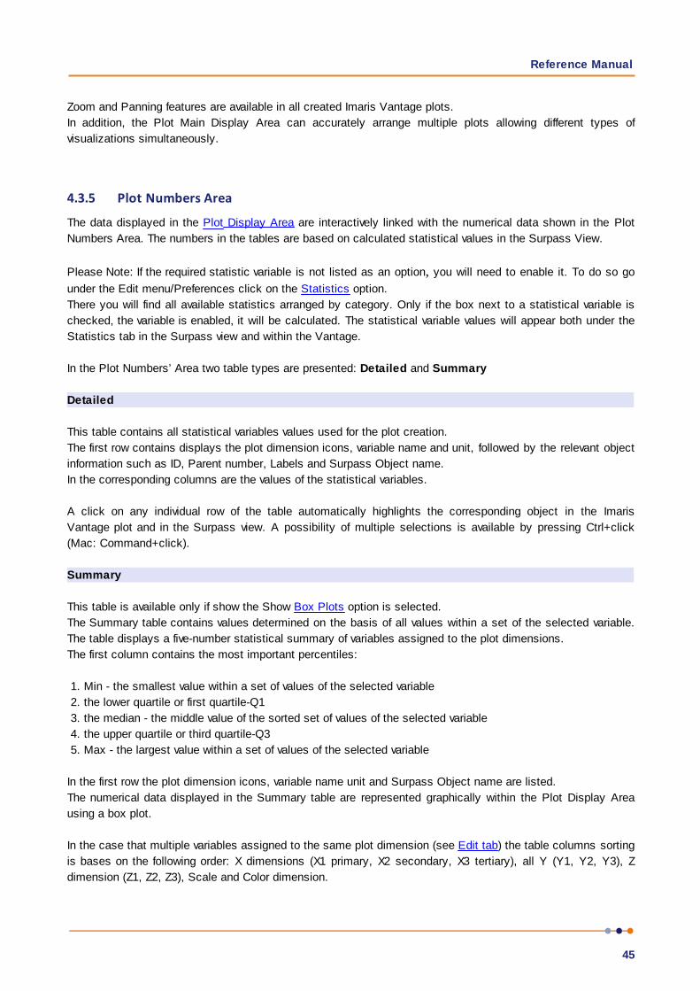
Reference Manual

45

Zoom and Panning features are available in all created Imaris Vantage plots.

In addition, the Plot Main Display Area can accurately arrange multiple plots allowing different types of

visualizations simultaneously.

4.3.5 Plot Numbers Area

The data displayed in the Plot Display Area are interactively linked with the numerical data shown in the Plot

Numbers Area. The numbers in the tables are based on calculated statistical values in the Surpass View.

Please Note: If the required statistic variable is not listed as an option, you will need to enable it. To do so go

under the Edit menu/Preferences click on the Statistics option.

There you will find all available statistics arranged by category. Only if the box next to a statistical variable is

checked, the variable is enabled, it will be calculated. The statistical variable values will appear both under the

Statistics tab in the Surpass view and within the Vantage.

In the Plot Numbers’ Area two table types are presented: Detailed and Summary

Detailed

This table contains all statistical variables values used for the plot creation.

The first row contains displays the plot dimension icons, variable name and unit, followed by the relevant object

information such as ID, Parent number, Labels and Surpass Object name.

In the corresponding columns are the values of the statistical variables.

A click on any individual row of the table automatically highlights the corresponding object in the Imaris

Vantage plot and in the Surpass view. A possibility of multiple selections is available by pressing Ctrl+click

(Mac: Command+click).

Summary

This table is available only if show the Show Box Plots option is selected.

The Summary table contains values determined on the basis of all values within a set of the selected variable.

The table displays a five-number statistical summary of variables assigned to the plot dimensions.

The first column contains the most important percentiles:

1. Min - the smallest value within a set of values of the selected variable

2. the lower quartile or first quartile-Q1

3. the median - the middle value of the sorted set of values of the selected variable

4. the upper quartile or third quartile-Q3

5. Max - the largest value within a set of values of the selected variable

In the first row the plot dimension icons, variable name unit and Surpass Object name are listed.

The numerical data displayed in the Summary table are represented graphically within the Plot Display Area

using a box plot.

In the case that multiple variables assigned to the same plot dimension (see Edit tab) the table columns sorting

is bases on the following order: X dimensions (X1 primary, X2 secondary, X3 tertiary), all Y (Y1, Y2, Y3), Z

dimension (Z1, Z2, Z3), Scale and Color dimension.

IMARIS

46

To sort the columns click on the arrow in the column heading. Click again to reverse the sorting.

Exporting Data

Export Button- Export All Statistics to File.

By selecting the Export icon , all of the data that appears in the selected table will be exported.

A click on the Export icon opens the Export Statistics window.

To export data select the file name and the file type (Comma Separated Values *.csv, Excel file *.xls, or Excel

XML *.xlm).

If you select MS Excel as file type, the program starts automatically.

4.4 Creation WizardA Plot Creation Wizard is a component of the Plot Property Area that guides you through a sequence of plot

creating dialogs. It leads you step by step through the process of selecting object categories, source data, plot

type and the various dimension options.

To create a plot, you must first create a Surpass object. The object statistical data will be used for the plot

creation.

Please Note: If the required statistic variable is not listed as an option, you will need to enable it. To do so go

under the Edit menu/Preferences click on the Statistics option.

There you will find all available statistics arranged by category. Only if the box next to a statistical variable is

checked, the variable is enabled, it will be calculated. The statistical variable values will appear both under the

Statistics tab in the Surpass view and within the Vantage.

The statistical values of the object Spots, Surfaces, Cells, and Filaments could be used to create the Vantage

plots.

To start Imaris Vantage creation wizard follow these steps:

1. Create and select the object in the Surpass tree

2. In the Toolbars, click on the Imaris Vantage icon.

3. Imaris Vantage is instantly started.

The wizard shows a list of all available input components for Imaris Vantage plots.

Select one of the input components from the list (Spots , Surfaces , Cells , or Filaments ).

In the next step of the Creation Wizard, specify the plot type that you want to use.

Then assign the selected statistical variables to the plot dimensions.

Click on the Finish button and the Vantage plot is displayed in the viewing area.

To insert a new Imaris Vantage object, click the Imaris Vantage icon to instantly generate a new Plot Creation

Wizard.

Please note that only the currently selected component is shown in the plot Main Display Area.

4.4.1 Source Data

All statistical values associated with one object type are grouped in one category. Each category has an

associated button with graphical indications of Category type.

Reference Manual

47

In Vantage there are the following categories: Spots , Surfaces , Cells and Filaments . The

category buttons allow you to choose the object type for the Vantage plot creation. The category icon is active

as long as surpass component is created.

Clicking on the Category button selects the corresponding category. According to the selection, all available

source objects data are listed.

Based on your selection, the Vantage tree in the Plot Input Data area displays a list of all source data you

added.

To remove an object data from the plot creation wizard, deselect the checkbox next to the object name or use

the delete button.

Please note: If multiple objects are selected in the first step of the creation wizard, the Gallery plot

type is not active in the next step of Creation wizard.

To insert a new Imaris Vantage plot, click the Imaris Vantage icon.

Load Plots Settings

This option lets you use identical creation parameters for multiple plots.

The option Load Plots Settings is only available if the set of the plot’s creation parameters has already been

saved using the Remember Parameters button under the Rebuild Tab.

When the wizard is started, all stored creation parameters, corresponding to the chosen object wizard, are

automatically loaded. The stored parameters contain all the settings, options, and parameters required for plot

creation.

After selecting the Load Plots Settings option, the Load Parameters drop-down list appears, Expand the list by

clicking on it. The list shows all the creation parameters sets that have been saved previously, according to the

chosen object. Simply load your chosen parameters set, by clicking on it, and run the wizard as you have

preset, without again defining all its possible options.

Another option is to customize each creation step to meet your specific needs by modifying some parts of the

wizard independently - e.g. the same plot type, with a different plot value selection.

4.4.2 Plot Setup

A Category identifies, gathers and summarizes the set of statistical values’ calculations of the particular ObjectType. Statistical values associated with one particular object type are grouped together in one category. Each

Category has its own button, which graphically indicates the Category type. In Imaris there are following Filter Categories: Surfaces , Surface Tracks , Spots , Spots Tracks ,

Dendrites , Dendrites Tracks , Filaments , Filament Tracks , Spines , Spine Tracks , Points

, Point Tracks , Cells , Cell Tracks , Nucleus , Nucleus Tracks , Vesicles and Vesicles

Tracks . These buttons allow you to choose the Category and determine the list of displayed statistical variables. By

clicking one of these buttons the corresponding category is selected and the list of statistical variables will be

displayed accordingly.

Please note: In Imaris Vantage, only one Object Type Category can be chosen.

Plot Type

Select the plot type you want to create from the plot type’s icons.

XYZ

IMARIS

48

Gallery

Time Plots

Scatter Plots

To view all options of the selected plot type click on the plot type icon and view the available plot subtypes.

To select a plot type, click the plot type, and then click on the plot subtype that you want.

By XYZ, Time and Scatter Plots each plot dimension represents one selected statistical variable. By default,

these plot types could show up to five statistical variables.

The choices of the available statistical variables for the selected object appear in a drop-down list.

To assign it to the selected Plot Value, select one statistical variable from the list.

Imaris Vantage plots allow you to select the same component for multiple plots.

Plot Values

Display the statistical variables’ name currently being assigned to the chosen plot dimension.

XYZ, Time and Scatter Plots show five options for the plot dimensions: X, Y, Z, Scale and Color.

Gallery plots, a selected statistical value is used to sort the objects. The values specified in the column or row

fields, define the number of panels to be displayed. In addition, Scale and/or Color could be chosen as a plot

dimensions.

The statistical variables for the Vantage can be chosen from the drop-down list. Click on the list and it offers a

set of all available statistical variables for the selected object. To select a particular statistical variable, click on

its name in the list and then the selected statistical variables will be assigned to the chosen plot dimension.

The exclamation mark sign indicates that the listed statistical parameter does not contain any value.

Please note: When creating a plot in the creation wizard, only one variable can be assigned to the chosen plot

dimension. However, when a plot creation wizard is completed, under the Edit tab, multiple variables could be

assigned to X, Y and Z plot dimensions.

X, Y and Z

Selecting the statistical variable for the X, Y and Z Plot Values define the three-dimensional space of the

Vantage plots. The position of the objects within the plot depends on the values of the variables assigned to the

X, Y and Z.

The Z-dimension initially points towards the viewer, outward from the screen.

For each Plot type, you can optionally provide an additional statistical variable to individually specify the objects

size, color or a combination of these features.

Scale

If you want to vary the object size across your plots, you need to specify the statistical variable for the Scale

dimension. The value of the variable selected for the Scale dimension determines the relative size of the object

within the plot.

Initially all the object dimensions are normalized and then the values of the Scale statistical variable is assigned

to the object. The lowest value of the selected statistical variable correspond to 0.25 of the normalized object

Reference Manual

49

size, while the highest value of the selected variable is mapped with the 1.25 of the normalized object size. The

new values are mapped, providing a new dimension for each object, without altering object shape parameters.

Please Note: Assigning the statistical variable for the Scale plot dimension is only appropriate when

the size of the created object doesn’t play a biological role.

Color

If you want to vary the object’s color across your plots, you need to specify the statistical variable for the Color

dimension. The values of the selected variable will determine the color of the object within the plot.

This scalar information of the selected variable is converted into colors using the colormap. The first color of the

selected color map is set to the lowest value of the selected statistical variable, while the highest value of the

selected variable is mapped with the last color.

Show All Time Points

Select this box and the created objects are shown for all time points.

Show Box Plots

Select this box and in the viewing area, the box plots are displayed for the selected plot dimensions.

In addition, in the Summary table in the Plot Numbers’ Area, all statistical summary numbers are show for all

plot dimensions.

Under the Edit tab, you can modify the display of the summary statistical values for individual plot dimension.

4.4.2.1 Box PlotA box plot summarizes the data of the selected statistical variable to only five numbers. It is a convenient way

to illustrate graphically large group of statistical data through their summaries: the minimum, lower quartile

(Q1), median, upper quartile (Q3), and maximum.

The central box represents the values from the lower Q1 to upper quartiles Q3 quartile (25 to 75 percentile

respectively).

The line within the box is indicates the median value. A straight lines extending from the ends of the box

represent the maximum and minimum values.

In the viewing area box plots can be drawn in all 3 plot dimensions for multiple variables.

If Vantage plot is composed of multiple objects, in the viewing area a separate box for each data set is created.

Box Plot is a useful tool offering several benefits to help you improve understanding of the data:

1. A quick visual summary that easily handles extremely large amount of data and shows range, spread and

median value of the selected variable values.

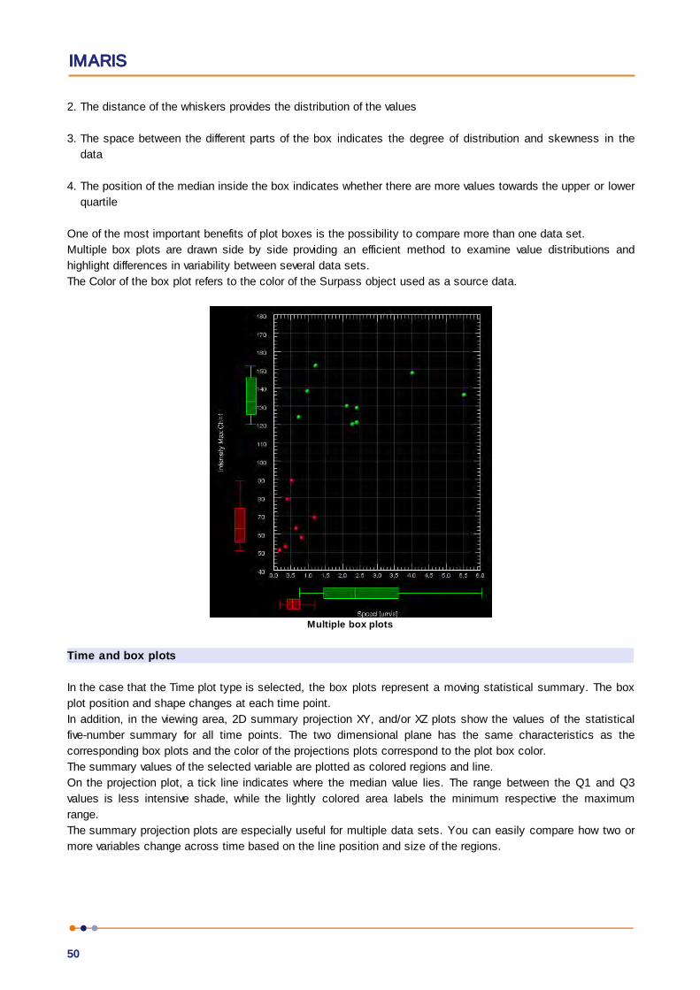
IMARIS

50

2. The distance of the whiskers provides the distribution of the values

3. The space between the different parts of the box indicates the degree of distribution and skewness in the

data

4. The position of the median inside the box indicates whether there are more values towards the upper or lower

quartile

One of the most important benefits of plot boxes is the possibility to compare more than one data set.

Multiple box plots are drawn side by side providing an efficient method to examine value distributions and

highlight differences in variability between several data sets.

The Color of the box plot refers to the color of the Surpass object used as a source data.

Multiple box plots

Time and box plots

In the case that the Time plot type is selected, the box plots represent a moving statistical summary. The box

plot position and shape changes at each time point.

In addition, in the viewing area, 2D summary projection XY, and/or XZ plots show the values of the statistical

five-number summary for all time points. The two dimensional plane has the same characteristics as the

corresponding box plots and the color of the projections plots correspond to the plot box color.

The summary values of the selected variable are plotted as colored regions and line.

On the projection plot, a tick line indicates where the median value lies. The range between the Q1 and Q3

values is less intensive shade, while the lightly colored area labels the minimum respective the maximum

range.

The summary projection plots are especially useful for multiple data sets. You can easily compare how two or

more variables change across time based on the line position and size of the regions.

Reference Manual

51

Time box plots

4.4.2.2 XYZ Plot TypeA XYZ plot is used to show the spatial relationship between the selected statistical variables.In XYZ plot type

the X, Y and Z Plot Values are predetermined variables, fixed and assigned to the object X, Y and Z position.

To uncover other structural connections, an additional statistical variable could be assigned as a Plot value.

To add another dimension to the plot, a fourth or fifth variable can be correlated to the color or size of the plotted

object, or a combination of these features.

Scale



within the plot.

Color


dimension. The values of the selected variable will determine the color of the object within the plot. This scalar

information of the selected variable is converted into colors using the colormap.

Plot Dimension

To select the statistical variable for the chosen plot dimensions click on the Plot Values list. This list offers a


its name in the list and the selected variables will then be assigned to the chosen plot dimension.


The following XYZ plot types are available:

Assigned Plot

Dimensions

Icons

Position X, Y

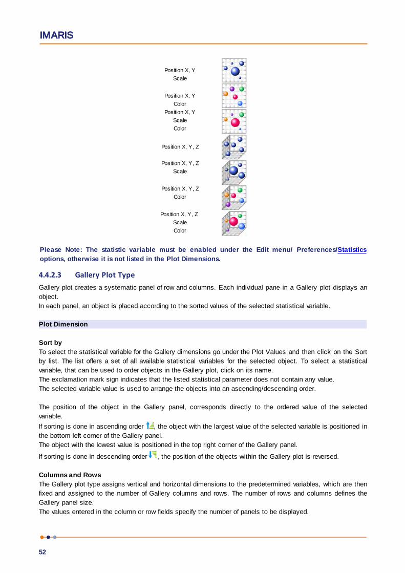
IMARIS

52

Position X, Y

Scale

Position X, Y

Color

Position X, Y

Scale

Color

Position X, Y, Z

Position X, Y, Z

Scale

Position X, Y, Z

Color

Position X, Y, Z

Scale

Color

Please Note: The statistic variable must be enabled under the Edit menu/ Preferences/Statistics

options, otherwise it is not listed in the Plot Dimensions.

4.4.2.3 Gallery Plot TypeGallery plot creates a systematic panel of row and columns. Each individual pane in a Gallery plot displays an

object.

In each panel, an object is placed according to the sorted values of the selected statistical variable.

Plot Dimension

Sort by

To select the statistical variable for the Gallery dimensions go under the Plot Values and then click on the Sort

by list. The list offers a set of all available statistical variables for the selected object. To select a statistical

variable, that can be used to order objects in the Gallery plot, click on its name.


The selected variable value is used to arrange the objects into an ascending/descending order.

The position of the object in the Gallery panel, corresponds directly to the ordered value of the selected

variable.

If sorting is done in ascending order , the object with the largest value of the selected variable is positioned in

the bottom left corner of the Gallery panel.

The object with the lowest value is positioned in the top right corner of the Gallery panel.

If sorting is done in descending order , the position of the objects within the Gallery plot is reversed.

Columns and Rows

The Gallery plot type assigns vertical and horizontal dimensions to the predetermined variables, which are then

fixed and assigned to the number of Gallery columns and rows. The number of rows and columns defines the

Gallery panel size.

The values entered in the column or row fields specify the number of panels to be displayed.

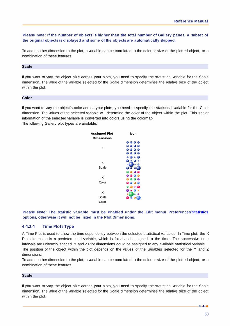
Reference Manual

53

Please note: If the number of objects is higher than the total number of Gallery panes, a subset of

the original objects is displayed and some of the objects are automatically skipped.

To add another dimension to the plot, a variable can be correlated to the color or size of the plotted object, or a

combination of these features.

Scale



within the plot.

Color




The following Gallery plot types are available:

Assigned Plot

Dimensions

Icon

X

X

Scale

X

Color

X

Scale

Color

Please Note: The statistic variable must be enabled under the Edit menu/ Preferences/Statistics

options, otherwise it will not be listed in the Plot Dimensions.

4.4.2.4 Time Plots TypeA Time Plot is used to show the time dependency between the selected statistical variables. In Time plot, the X

Plot dimension is a predetermined variable, which is fixed and assigned to the time. The successive time

intervals are uniformly spaced. Y and Z Plot dimensions could be assigned to any available statistical variable.

The position of the object within the plot depends on the values of the variables selected for the Y and Z

dimensions.

To add another dimension to the plot, a variable can be correlated to the color or size of the plotted object, or a

combination of these features.

Scale



within the plot.

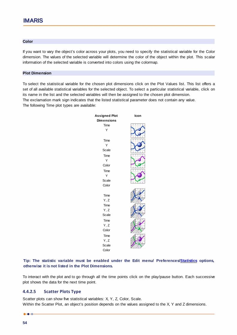
IMARIS

54

Color




Plot Dimension

To select the statistical variable for the chosen plot dimensions click on the Plot Values list. This list offers a




The following Time plot types are available:

Assigned Plot

Dimensions

Icon

Time

Y

Time

Y

Scale

Time

Y

Color

Time

Y

Scale

Color

Time

Y, Z

Time

Y, Z

Scale

Time

Y, Z

Color

Time

Y, Z

Scale

Color

Tip: The statistic variable must be enabled under the Edit menu/ Preferences/Statistics options,

otherwise it is not listed in the Plot Dimensions.

To interact with the plot and to go through all the time points click on the play/pause button. Each successive

plot shows the data for the next time point.

4.4.2.5 Scatter Plots TypeScatter plots can show five statistical variables: X, Y, Z, Color, Scale.

Within the Scatter Plot, an object’s position depends on the values assigned to the X, Y and Z dimensions.

Reference Manual

55

To add another dimension to the plot, a fourth or fifth variable can be correlated to the color or size of the plotted

object, or a combination of these features.

Scale



within the plot.

Color




Plot Dimension

To select the statistical variable for the chosen plot dimensions click on the Plot Values list. The list offers a




The following Scatter plot types are available:

Assigned Plot

Dimensions

Icons

X,Y

X, Y

Scale

X, Y

Color

X, Y

Scale

Color

X, Y, Z

X, Y, Z

Scale

X, Y, Z

Color

X, Y, Z

Scale

Color

Tip: The statistic variable must be enabled under the Edit menu/ Preferences/Statistics options,

otherwise it is not listed in the Plot Dimensions.

IMARIS

56

4.5 Settings TabDepending on the object selection the content under the Settings tab differs.

Please click the appropriate link given below:

Cells

Filaments

Spots

Surfaces

4.6 Rebuild TabThe rebuild option is useful to store your own customized plots’ parameters and re-use them. It also enables

you to share the plot creation parameters with other people, allowing them to use an identical set of parameters

to perform their own analysis and have them perform their own analysis by using identical set of parameters.

Imaris stores the list of plot creation parameters. Select from the list, which step of the Plot Creation Wizard

you want to re-enter.

Source Data

Plot Setup

Rebuild Button

Clicking on this button re-starts the wizard.

Creation Parameters

The Creation Wizard saves parameters so that the Imaris Vantage plot creation can be repeated, and the

process of re-creating complex yet standardized plots may be avoided.

The Creation Parameters are listed in the table.

Refer to Store Creation parameters

Preference

When you save the Creation Parameter file, it is automatically added to the list that is displayed under the Edit/

Preference/Vantage Plots

4.7 Store Creation ParametersStore Parameters Button

The Store Parameters button allows you to save the complete set of the creation parameters and the relevant

settings shown in the list. Storing the parameters allows them to be easily reused, modified, or exchanged

between users. Once you have saved the creation parameters, you can reuse them in any new creation wizard.

All the settings and values required to apply the same parameters to the new data set are automatically loaded

and available as a Load Parameter option in the appropriate plot creation wizard.

When you save the Creation Parameter file, it is automatically added to the list which is displayed under the

Edit/Preference/Creation Parameters.

Clicking on the Remember Parameters Button opens the Store Creation Parameter window.

Store Creation Parameter Window

Enter a name for the Creation Parameter set. This name then identifies the Creation Parameter item, in the

Reference Manual

57

Creation Parameter list, used in the Edit/Preference/Creation Parameters and would be used as default name in

the subsequent creation wizard algorithms.

Save all of the attributes of your favorite graph style under the Rebuild tab. Add greater speed and efficiency to

your analysis by quickly recalling an existing graph type, and then apply this style to your current data set

4.8 View TabUnder the View Tab you can determine the relative size of the objects, their orientation and their position within

the Plots.

-/ + Button

Selecting this button changes the objects size within the View Area by simultaneously changing the Scale

values for all X,Y and Z plot dimensions.

Scaling is measured in percent, starting from 100% as the initial object size.

Plus Button

The size of the object is increased by 10% every time the Plus button is pressed.

Also, every time the Plus button is clicked, under the Edit tab, the number in the Scaling field for the X, Y andZ plot dimensions is reduced by 10%.

Minus Button

The size of the object is reduced by 10% every time the Minus button is pressed.

Also, every time the Minus button is clicked, under the Edit tab, the number in the Scaling field for the X, Yand Z plot dimensions is increased by 10%.

Scale Objects to Same Size

Select this button to map all objects with equal size distribution.

All objects within the plot are scaled to the largest object

Orientation Horizontal /Vertical slider

To rotate the objects horizontally/vertically and change the object orientation use the sliders.

Align Objects

Select this box to align objects relative to each other.

The objects are aligned along a horizontal or vertical line which represents their original positions.

Reset Orientation button

Select this button to set an original orientation of the objects.

4.9 Edit TabThe Edit Tab offers the flexibility to customize every detail of your plot appearance by interactively modifying the

various plot elements. It gives you independent control of plot dimensions.

Under the Edit Tab, you can adjust the following characteristics of a plot: modify the number and type of the

IMARIS

58

assigned statistical variable to the plot dimension, change the position and scale of the objects, define the

objects’ binning, alter limits and appearance of the plot dimension scale, and add the annotations’ labels and

text.

Categories

A Category identifies, gathers and summarizes the set of statistical values’ calculations for that particularObject Type. Statistical values associated with one particular object type are grouped together in one category.

Each Category has its own button, which graphically indicates the Category type. In Imaris there are the following Filter Categories: Surfaces , Surfaces Tracks , Spots , Spots Tracks ,

Dendrites , Dendrites Tracks , Filaments , Filaments Tracks , Spines , Spine Tracks , Points

, Points Tracks , Cells , Cells Tracks , Nucleus , Nucleus Tracks , Vesicles and Vesicles

Tracks . These buttons allow you to choose the Category and determine the list of displayed statistical variables. By

clicking one of these buttons the corresponding category is selected and the list of statistical variables will be

displayed accordingly.

Please note: In Imaris Vantage, only one Object Type Category can be chosen.

Depending on the selected Plot type the content under the Edit tab differs.

XYZ

Gallery

Time Plot

Scatter Plot

4.9.1 XYZ, Time and Scatter Plots

Dimensions

The Edit tab gives you independent control of plot dimensions.

Within the Dimensions window, a list displays the checkbox, icon and assigned variable name for all plot

dimensions.

In the list dimensions appear in the following order: X1, X2, X3, Y1, Y2, Y3, Z1, Z2, Z3, Scale and Color.

Selecting or de-selecting the box next to the plot dimension controls its visibility in the viewing area.

The following table gives an overview of the plot dimensions icons:

Plot Dimension Icon

X

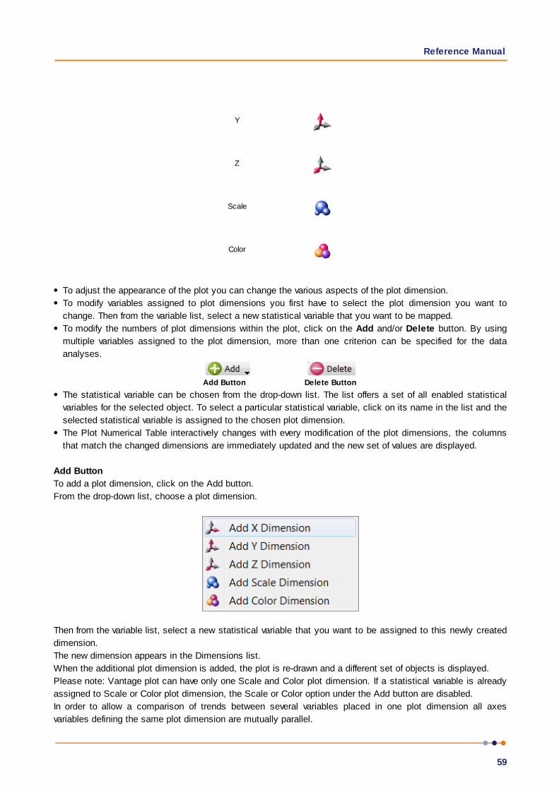
Reference Manual

59

Y

Z

Scale

Color

To adjust the appearance of the plot you can change the various aspects of the plot dimension.

To modify variables assigned to plot dimensions you first have to select the plot dimension you want to

change. Then from the variable list, select a new statistical variable that you want to be mapped.

To modify the numbers of plot dimensions within the plot, click on the Add and/or Delete button. By using

multiple variables assigned to the plot dimension, more than one criterion can be specified for the data

analyses.

Add Button Delete Button

The statistical variable can be chosen from the drop-down list. The list offers a set of all enabled statistical

variables for the selected object. To select a particular statistical variable, click on its name in the list and the

selected statistical variable is assigned to the chosen plot dimension.

The Plot Numerical Table interactively changes with every modification of the plot dimensions, the columns

that match the changed dimensions are immediately updated and the new set of values are displayed.

Add Button

To add a plot dimension, click on the Add button.

From the drop-down list, choose a plot dimension.

Then from the variable list, select a new statistical variable that you want to be assigned to this newly created

dimension.

The new dimension appears in the Dimensions list.

When the additional plot dimension is added, the plot is re-drawn and a different set of objects is displayed.

Please note: Vantage plot can have only one Scale and Color plot dimension. If a statistical variable is already

assigned to Scale or Color plot dimension, the Scale or Color option under the Add button are disabled.

In order to allow a comparison of trends between several variables placed in one plot dimension all axes

variables defining the same plot dimension are mutually parallel.

IMARIS

60

Please note: From a practical concern, it is most likely very difficult to interpret a graph with more than 3 X, Y,

and Z axis and therefore Imaris restricts the number of variables assigned to one plot dimension to three.

Delete Button

To remove an unwanted plot dimension, select it and click the Delete button. The selected plot dimension is

deleted from the plot.

Plot

The statistical variable can be chosen from the drop-down list. The list offers a set of all enabled statistical

variables for the selected object type. To select a particular statistical variable, click on its name in the list and

then this selected statistical variable is assigned to the chosen plot dimension.

To remove the assigned plot dimension from the viewing area, deselect the checkbox next to the plot dimension

name.

The Plot Number Area interactively changes with every modification of the plot dimensions, the columns that

match the changed dimensions are immediately updated and the new sets of values are displayed.

Scale

A scale function specifies how the scale of each plot dimension should be determined from the value of the

selected statistical variable.

As the values of the selected variable may be of different magnitudes, during the plot creation, the offset and

scaling values are automatically calculated based on each of the selected variables values.

After automatic scaling, the ranges appear to be the same for all of the objects currently being visualized.

The Scale value provides you with options to adapt how the plot dimensions are scaled.

To change the scaling of the selected plot dimension and enter a number in the Scale field.

The entered Scale value multiplies the initially calculated values of the selected plot dimension by the value

entered in the Scale field.

Offset

This parameter is used to reposition the objects from their original position within the plots.

Offsetting objects is useful when you have more than one object in the same position and you want to evenly

distribute the objects in a particular direction. For example, if you have many objects that you want to shift

horizontally in a straight line, you can specify the value, in increments, in the Offset field for the selected X

dimension.

The offset values change the object’s originally assigned value. This new value is calculated by adding the

entered offset value to the value of the selected statistical variable.

The offset value can be positive or negative.

For the X plot dimension, positive offset numbers move the objects to the right, and negative numbers move

them to the left. For the Y plot dimension, positive offset numbers move the objects up , and negative numbers

move them down.

The offset value is given in the same units as the selected statistical variable assigned to the selected plot

dimension.

Clicking this arrow sets the Scale and Offset back to the original values.

Limit Min Limit Max

Reference Manual

61

During plot creation, the range is automatically adjusted to the actual lowest and highest value of the selected

variable.

Min: This is the smallest value of the selected variable to be displayed.

Max: This is the largest value of the selected variable to be displayed.

It is possible to change the Max limit and/or Min limit of the selected plot dimension by entering the values in

the Limit Min /Max fields.

Enter a value to the Limit Min /Max to specify the new minimum/maximum values for the selected plot

dimension.

Clicking this arrow sets the Limit Min /Max back to the original values.

Bin Size

Binning allows you to sort your data into different groups or bins. The Binning size value divides a plot into a

specific number of groups and specifies the new locations of the objects by distributing them into the different

bins according to the value of the selected variable.

Gamma

The Gamma function allows you to individually manipulate the appearance of the range of the selected variable.

The default value of the Gamma is 1, indicating that the range between the lowest and highest value of the

selected variable is extrapolated in a linear mode to the full range of the data set.

If the entered value is different than 1, the linear mode is transferred to a nonlinear mode.

Entering the Gamma values higher than 1, will result in a plot in which the range of the object with the lower

values will appear to increase relative to the range of the object with higher values.

Alternatively, entering the Gamma values smaller than 1, will result in a plot in which the range of the object

with higher values will appear to increase relative to the range of the object with lower values.

The change is directly visible in the viewing area.

Clamp Limits

If this box is selected, the object outside the plots limits (determined by the frame and range settings) will be

repositioned within the limits.

The object with the higher value will be assigned the max value of the selected variable, while the object with

the lower value will be assigned the minimum value.

Show Box Plots

Select this box and in the viewing area, the box plots are displayed for the selected plot dimension.

Auto Adjust

Click on this button and the parameters under the Edit tab are returned to the original values.

Load Colormap

Click on the button Colormap to display a large number of predefined colormaps. If the default colormap

(Spectrum) is not appropriate, you can change it by clicking on the drop-down list. The list gives a preview of

IMARIS

62

what different colormaps look like.



4.9.2 Gallery

Sort by:

To modify the statistical variable for the Gallery dimensions go to Plot Values and then click on the Sort by

list.

The icons indicates the sort order in the Gallery, ascending or descending order

Cell Columns /Row

To readjust the numbers of panels to be displayed in the Gallery enter the values in the column or row fields.

Skip

The entered value defines the number of displayed objects by defining the skip interval. To display every second

object set the value to 1, or to display every third object set the value to 2.

Offset

Adjusting the Offset value is useful when the number of objects is higher than the total number of Gallery

panes.

The offset value specifies the first object to be placed in the Gallery. To display first object, set the offset value

to 0. To start with the 10th ordered object, set the value to 10.

The Skip and Offset value regulate and limit the Gallery display to a certain number of the displayed objects. In

combination, these two values define the subset of the originally ordered objects.

Offset Skip Displayed Objects in the Gallery

0 0 all objects

10 0 10th 11th 12th 13th ...

20 15 20th 35th 50th 65th ...

Cell With/Height

The Gallery panel size is equal to the settings in the width/height numerical fields.

Plot Dimensions

The Edit tab gives you independent control of plot dimensions.

Select a plot dimension from the list of icons:

Reference Manual

63

Plot Dimension Icon

Scale

Color

Selecting or de-selecting the box next to the plot dimension name controls its visibility in the viewing area.

To adjust the appearance of the plot you can change the various aspects of the plot dimension.

To modify the existing condition, you have to first select the plot dimension you want to change.

To assign a different statistical variable to the current dimension, select a new statistical variable that you

want to be mapped.

To incorporate a new plot dimension into the plot, select the preferred dimension and assign a new statistical

variable.

The statistical variable can be chosen from the drop-down list. The list offers a set of all available statistical

variables for the selected object. To select a particular statistical variable, click on its name in the list and

then this selected statistical variable is assigned to the chosen plot dimension.

To remove the assigned plot dimension from the viewing area, deselect the checkbox next to the plot

dimension name.

The Plot Numerical Table interactively changes with every modification of the plot dimensions, the columns

that match the changed dimensions are immediately updated and the new sets of values are displayed.

Offset

This parameter is used to reposition the objects from their original position within the plots.

Offsetting objects is useful when you have more than one object in the same position and you want to evenly

distribute the objects in a particular direction. For example, if you have many objects that you want to shift

horizontally in a straight line, you can specify the value, in increments, in the Offset field for the selected X

dimension.

The offset values change the object’s originally assigned value. This new value is calculated by adding the

entered offset value to the value of the selected statistical variable.

The offset value can be positive or negative.

For the X plot dimension, positive offset numbers move the objects to the right, and negative numbers move

them to the left. For the Y plot dimension, positive offset numbers move the objects down, and negative

numbers move them up.

The offset value is given in the same units as the selected statistical variable assigned to the selected plot

dimension.

Scale

A scale function specifies how the scale of each plot dimension should be determined from the value of the

selected statistical variable.

As the values of the selected variables may be of different magnitudes, during the plot creation, the offset and

scaling values are automatically calculated based on each of the selected variable values.

After the automatic scaling, the ranges appear to be the same for all of the objects currently being visualized.

The Scale value provides you with options to adapt how the plot dimensions are scaled.

To scale the selected plot dimension enter a number in the Scale field.

IMARIS

64

The entered Scale value multiplies the initially calculated values of the selected plot dimension by the value

entered in the Scale field.

Clicking this arrow sets the Scale and Offset back to the original values.

Limit Min Limit Max

During the plot creation, the range is automatically adjusted to the actual lowest and highest value of the

selected variable.

It is possible to change the max limit and/or min limit of the selected plot dimension by entering the values in

the Limit Min /Max fields.

Enter a value to the Limit Min /Max to specify the new minimum/maximum values for the selected plot

dimension.

Clicking this arrow sets the Limit Min /Max back to the original values.

Bin Size

Binning allows you to sort your data into different groups or bins. The Binning size value divides a plot into a

specific number of groups and specifies the new locations of the objects by distributing them into the different

bins according to the value of the selected variable.

Gamma

The Gamma function allows you to individually manipulate the appearance of the range of the selected variable.

The default Gamma value is 1, indicating that the range between the lowest and highest value of the selected

variable is extrapolated in a linear mode to the full range of the data set.

If the entered value is different than 1, the linear mode is transferred to a nonlinear mode.

Entering Gamma values higher than 1, will result in a plot in which the range of the object with the lower values

will appear to increase relative to the range of the object with higher values.

Alternatively, entering Gamma values smaller than 1, will result in a plot in which the range of the object with

higher values will appear to increase relative to the range of the object with lower values.

The change is directly visible in the viewing area.

Clam Limits

If this box is selected the object outside the plots limits (determined by the frame and range settings) will be

repositioned within the limits.

The object with the higher value will be assigned the max value of the selected variable, while the object with

the lower value will be assigned the minimum value.

Auto Adjust

Click on this button and the parameters under the Edit tab are returned to the original values.



Reference Manual

65

4.10 Frame TabCommon aspects of all frames, such as the thickness and color of frame, grid tickmarks and labels setting can

be controlled using this tab.

Box and Time Settings

Box

Check the parameter to display a box around the Frame.

Line Width

Adjust the box line width with the respective slider. Moving the slider to the left reduces the line width, moving it

to the right increase line width.

Shading

Check this parameter to display shading. Use the slider to adjust the shade contrast.

Shadow

The entire Scene can produce shadows on the three planes of the Frame object. Check this box to display the

shadows. Use the Shading slider (see above) to adjust the contrast. The rendering is done in real-time, and it

requires a high performance graphic board.

Time Colorbar

Only available if you work with a time data set. Check this box and the Time Colorbar appears in the lower left

corner of the viewing area.

Grid and Tick marks Settings

Grid

Check the box Grid to display a grid. Use the slider to adjust the grid width.

The Scale is shown/by a grid behind the object. The frame moves to stay behind the object as it is rotated. The

distance represented by each square in the grid, the scale bar, is in the bottom right corner of the screen.

Tickmarks

Check the box Tickmarks to display tickmarks on the edges of the frame.

Spacing

Specify the grid and tickmark spacing for the X, Y and Z plot dimensions.

The frequency of tick marks can be controlled by selecting the appropriate interval values from the drop-down

list.

Labels Settings

Axis Labels

Check the box Axis Labels to display the x, y, and z axes to clearly show the orientation of the object. If this

box is checked, the parameter Label Color and Label Font is available (see below).

Label Color

Only available if the parameter Axis Labels (see above) is checked. Click on the Color Editor window to change

the color of the label on the coordinate axes.

IMARIS

66

Label Font

Only available if the parameter Axis Labels (see above) is checked. Click on the Font Editor window to change

the font to label the coordinate axes.

Fix Decoration to Data Set

Check Fix Decoration to Data Set to fix the Frame to the same side when navigating the object.

4.11 Color TabPlease note: The color coding option is not available under the Vantage Color Tab.

RGB

The RGB color model is an additive color model in which Red, Green and Blue are combined together to

reproduce an array of colors. The color values may be changed either by clicking on the color wheel to select a

color, or by direct numeric entry for the Red, Blue or Green component (values range from 0 to 1).

Light reflection

Quality of the object material is further characterized by reflection properties:

Diffusion- diffuses reflection of a matte, uneven material.

Specular- defines reflection of highly reflective materials. The brighter a specular map is, the more shine is

applied to the object. The default setting is for no specular intensity.

Emission- light emitted from the material defines the self-illumination. The default setting is for no emission.

Transparency

Transparency defines the amount of light allowed to pass through an object. Click this tool to change the

percentage from 0% (complete opacity) to 100% (complete image transparency).

Palette

Palette- this option provides a system of preset colors organized into color schemes.

In the Palette, colors are labeled and grouped together. The scrolling window contains 14 color combination

groups (Custom, Artdeco, Autumn, Glass, Metal, Neon, Rococo, Santafe, Sheen, Silky, Spring, Summer,

Tropical, Winter). Examples of colors in a selected group are displayed in the attached rectangular area. If a

custom color has been defined on the RGB tab, it can be added to the Custom palette with the Add to Palette

button. After being added, these color palette choices are stored and can be used with other Imaris objects.

4.12 1D ViewVantage 1D View provides an effective way to view patterns and trends in statistical data in the form of one

dimensional scatter plots.

1D view lets you analyze data, and compare and derive relationships from one or more data sets. 1D View

provides a simpler means to analyze and view data sets (for example spots) than Vantage Objects View,

however many of the functions found in Objects View are the same and are described previously in Vantage

View. In addition the Statistics Tests tab provides powerful statistical tests for direct analysis of your data sets

within Imaris 1D View.

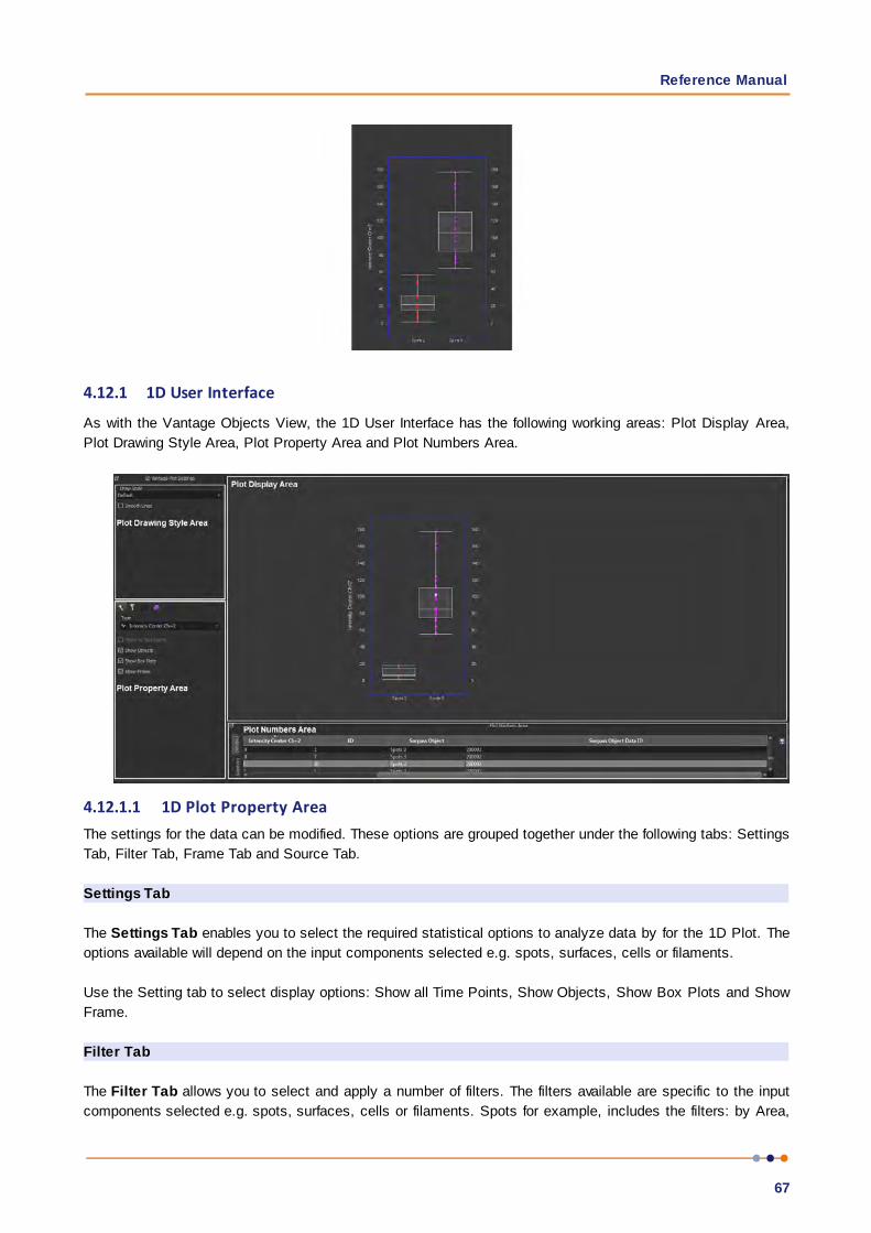
Reference Manual

67

4.12.1 1D User Interface

As with the Vantage Objects View, the 1D User Interface has the following working areas: Plot Display Area,

Plot Drawing Style Area, Plot Property Area and Plot Numbers Area.

4.12.1.1 1D Plot Property AreaThe settings for the data can be modified. These options are grouped together under the following tabs: Settings

Tab, Filter Tab, Frame Tab and Source Tab.

Settings Tab

The Settings Tab enables you to select the required statistical options to analyze data by for the 1D Plot. The

options available will depend on the input components selected e.g. spots, surfaces, cells or filaments.

Use the Setting tab to select display options: Show all Time Points, Show Objects, Show Box Plots and Show

Frame.

Filter Tab

The Filter Tab allows you to select and apply a number of filters. The filters available are specific to the input

components selected e.g. spots, surfaces, cells or filaments. Spots for example, includes the filters: by Area,

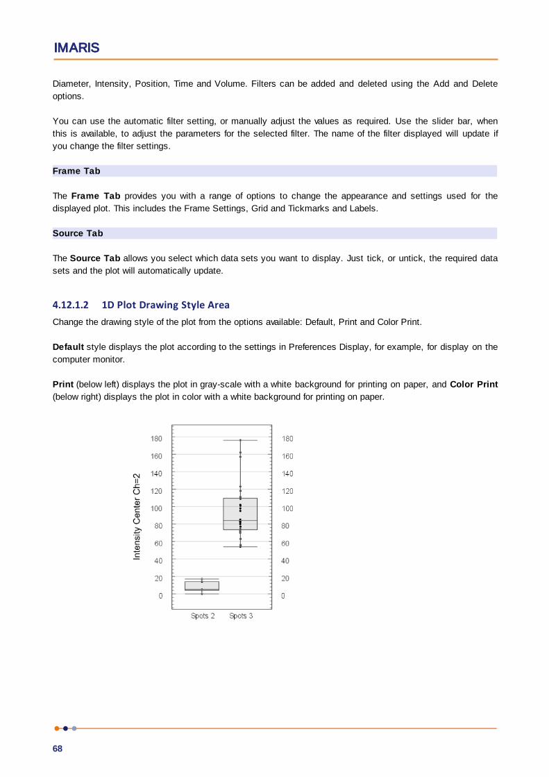
IMARIS

68

Diameter, Intensity, Position, Time and Volume. Filters can be added and deleted using the Add and Delete

options.

You can use the automatic filter setting, or manually adjust the values as required. Use the slider bar, when

this is available, to adjust the parameters for the selected filter. The name of the filter displayed will update if

you change the filter settings.

Frame Tab

The Frame Tab provides you with a range of options to change the appearance and settings used for the

displayed plot. This includes the Frame Settings, Grid and Tickmarks and Labels.

Source Tab

The Source Tab allows you select which data sets you want to display. Just tick, or untick, the required data

sets and the plot will automatically update.

4.12.1.2 1D Plot Drawing Style AreaChange the drawing style of the plot from the options available: Default, Print and Color Print.

Default style displays the plot according to the settings in Preferences Display, for example, for display on the

computer monitor.

Print (below left) displays the plot in gray-scale with a white background for printing on paper, and Color Print

(below right) displays the plot in color with a white background for printing on paper.

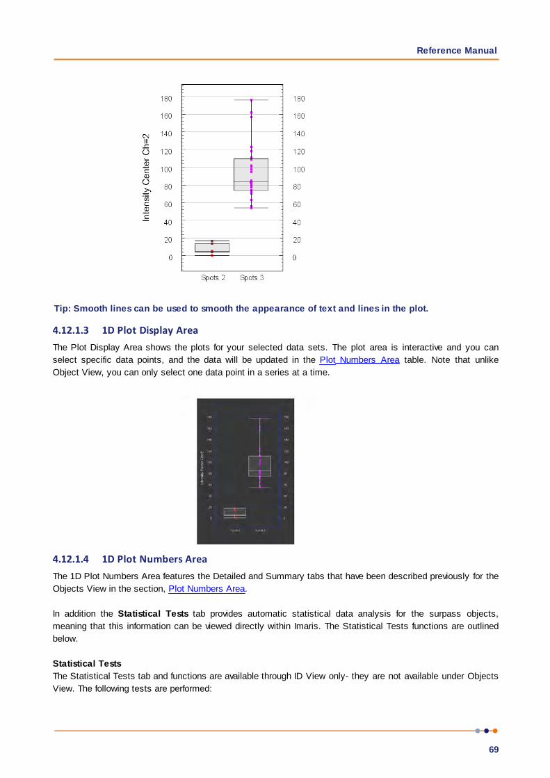
Reference Manual

69

Tip: Smooth lines can be used to smooth the appearance of text and lines in the plot.

4.12.1.3 1D Plot Display AreaThe Plot Display Area shows the plots for your selected data sets. The plot area is interactive and you can

select specific data points, and the data will be updated in the Plot Numbers Area table. Note that unlike

Object View, you can only select one data point in a series at a time.

4.12.1.4 1D Plot Numbers AreaThe 1D Plot Numbers Area features the Detailed and Summary tabs that have been described previously for the

Objects View in the section, Plot Numbers Area.

In addition the Statistical Tests tab provides automatic statistical data analysis for the surpass objects,

meaning that this information can be viewed directly within Imaris. The Statistical Tests functions are outlined

below.

Statistical Tests

The Statistical Tests tab and functions are available through ID View only- they are not available under Objects

View. The following tests are performed:

IMARIS

70

Test Summary

Wilcoxon-test

The Wilcoxon-test is also referred to as Mann-Whitney

test. The Wilcoxin-test enables you to determine

whether two sets of surpass data sets with ordinal data,

but without normalised distribution i.e. non-parametric,

are statistically different from each other.

t-test

The t-test enables you to test whether the mean of two

data sets (for small populations) are statistically

different from each other. With this test, there is an

option to assume that the variation between the surpass

data sets are the same, in this case a Welch’s t-test is

performed. If this is not the case, a Student’s t-test will

be performed.

f-test

The f-test enables you to test (the null hypothesis) that

the variance of two data sets are equal. This is done by

comparing the ratio of the variance between the two

surpass data sets.

Kolmogorov-Smirnov

test

The KS-test lets you determine if two data sets differ

significantly. The KS-test is distribution free.

The statistics are compared for the first of the surpass objects against the others in the list, and the results are

displayed in columns as shown in the example below. If the test does not meet the criteria to run, the reason

will be displayed.

As the statistics are compared for the first of the surpass objects against the others in the list, to change the

order of the data sets drag the items within the list to the required order. In the following example, "Spots Type

1" is compared against "Spots Type 2" and "Spots Type 3". "Spots Type 3" could be compared against "Spots

Type 1" and "Spots Type 2" by dragging it to the top of the list.

The settings for Statistical Tests can be viewed and edited e.g. confidence level or test type, using the

Settings button. This is a shortcut to Statistical Tests preferences.

Reference Manual

71

Note that data for each tab can be exported using the button when that tab is highlighted.

IMARIS

72

Section 5 File

The options available from the file menu will depend on the current view selected:

Arena Options

The following options can be selected from the File menu under Arena:

Batch Convert

Scene Viewer

Store Arena and

Restore Arena

Ctrl + Shift +

E

Ctrl + Shift +

I

Batch Queue Ctrl + Shift +

B

Preferences... Ctrl + P

List of recently opened

Surpass files

Exit Ctrl + Q

In other modes e.g. Surpass additional options are available and these will change according to what applies

to the current image.

Open... Ctrl + O

Open in a new

Window

Ctrl + Shift +

O

Revert to File Ctrl + R Use Revert to File to revert to the previously saved version of an image file.

Store Ctrl + S Use the Store and Store as options to save the current image file as

required.Store as

Export... Ctrl + E Use Export to save the image file to another location.

Import Scene The actual Imaris configuration (including Surpass Tree and all existing

Items) in the Surpass view is called Scene and can be stored in a Scene

file with the extension *.imx. The Scene can be loaded again to the same

data set or to another data set. For details please refer to Section Surpass

View - Overview - Scene File Concept.

Export Scene

Add Image... Ctrl + Shift + I Add an image into an Imaris Scene for multi-

image data sets. Please refer to Multi-image

See also:


5.1 Batch Convert ...With Batch Convert... (Imaris File Converter) you can convert various image file formats to the Imaris file format

*.ims. Select the menu entry Batch Convert... and the Imaris File Converter window displays. From the

Windows Start menu select "ImarisFileConverter".

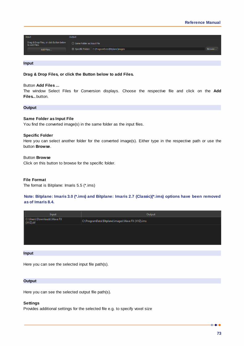
Reference Manual

73

Input

Drag & Drop Files, or click the Button below to add Files.

Button Add Files ...

The window Select Files for Conversion displays. Choose the respective file and click on the Add

Files...button.

Output

Same Folder as Input File

You find the converted image(s) in the same folder as the input files.

Specific Folder

Here you can select another folder for the converted image(s). Either type in the respective path or use the

button Browse.

Button Browse

Click on this button to browse for the specific folder.

File Format

The format is Bitplane: Imaris 5.5 (*.ims)

Note: Bitplane: Imaris 3.0 (*.ims) and Bitplane: Imaris 2.7 (Classic)(*.ims) options have been removed

as of Imaris 8.4.

Input

Here you can see the selected input file path(s).

Output

Here you can see the selected output file path(s).

Settings

Provides additional settings for the selected file e.g. to specify voxel size

IMARIS

74

Remove Selected and Remove All buttons

Click on these buttons to clear either a selected row or all rows in the table respectively.

Button Start All

Click on this button to start the conversion.

When the conversion starts, files are moved to the bottom table. This displays the progress of the conversion

for both read progress and write progress. It is possible to add new files and configure settings while a

conversion is running.

This then updates on completion of the process:

See also:

Imaris Menu - Open - Reader Configuration

Imaris Menu - Open - Settings

Imaris Menu - Export ... - Advanced Save Options

5.1.1 Preferences

Button Preferences

Click on this button to open the Preferences window.

Window: Preferences

Data Cache

Imaris utilizes advanced data caching mechanism that allows you to process images that are significantly

larger than the physical memory (RAM) installed in the computer system. This mechanism writes image data

blocks to the disk and reads them back into the physical memory when they are needed.

Cache File Paths displays the cache file location.

Please note: Setting the Cache File location to an unused disc, improves the performance when

working on larger images. This benefits greatly from a fast SSD with a minimum size of 10 times the

biggest data set, which will be used.

Reference Manual

75

Memory Limit (MB)

The value of Data cache limit controls the amount of data blocks Imaris will keep in memory at any time.

File Paths:

Display of the cache file paths.

Button Add

You can use the buttons to add file paths in the list.

Button Remove

You can use the buttons to remove file paths in the list.

Output Formats

If you want to extend the list of output formats you have to check the following parameter and enter a valid

license in the next step. Find your license number in Imaris as follows: Click on the menu Help, select the

menu entry Licenses and copy the license number (in the License Path at the bottom of the window, next to

last enter field).

Include Image Filenames

Select this option and the output file names are assigned by using a default-naming rule.

Suffix Alphabetic

The output file inherits the input file name followed by the successive alphabetic letter.

Suffix Numeric

The output file inherits the input file name followed by the number of the output files being created (consecutive

integer numbers).

All Imaris Output File Formats

Check this box to extend the output file formats.

License Location

Type in your license number or use the button Browse.

Button Browse

Click on this button and select the license path.

Button OK

Click on this button and all available Imaris output formats are available.

Standard formats:



Bitplane: Imaris 2.7 (Classic)(*.ims)

Additional formats:

Tiff (series)(*.tif *.tiff)

RGBA-Tiff (series)(*.tif *.tiff)

ICS file (*.ics *.ids)

Olympus: cell^R 1.1/standard (*.tif *.tiff)

IMARIS

76


Open Microscopy Environment Tiff (*.tif *.tiff)

BMP (series)(*.bmp)

See also:

Imaris Menu - Export ...

5.2 Store Arena and Restore ArenaStore Arena and Restore Arena allow you to manage your image data files and Arena tree structure.

Store Arena

Using Store Arena you can copy image files to the data storage location that has been set by the user under

Arena Preferences. This enables your Arena data files to be stored on a range of local and remote locations.

This includes HDD or SSD drives, and removable data storage devices such as USB memory sticks. When

using network server locations you will require authentication to access the network server- this is described in

Arena Preferences.

Default Data Storage location:

PC: C:\ProgramData\Bitplane\DataStorage

Mac: \Library\Bitplane\DataStorage

Arena Files are stored in .ims format. Files in other formats will be converted into .ims format as part of the

upload process.

Note that Store and Restore functions are not available if they have been disabled under Imaris

Administrator. This is to prevent overwriting files that may be used by more than one user, for

example, image files saved on a remote, network server location that may be accessed and

modified independently by different users.

There are three options:

Arena View only

Will store only image files currently within the Imaris data store.

Arena View + Local files

Will store image files within the Imaris data store and any other image files that are present on a local

(physical) drive.

Arena View + Local files and Remote files

Will store image files within the Imaris data store and any other image files on both local and remote locations.

Restore Arena

With Restore Arena you can restore image files in Arena View to the time of the last save. For example, if you

have deleted, or modified a file by accident.

Note that when the Restore Arena function is used, all image data in Arena will be overwritten as

the image data will be returned to that of the previous save.

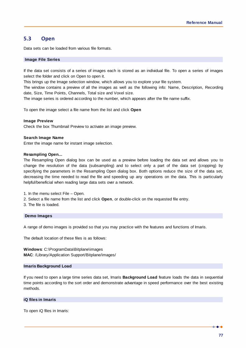
Reference Manual

77

5.3 OpenData sets can be loaded from various file formats.

Image File Series

If the data set consists of a series of images each is stored as an individual file. To open a series of images

select the folder and click on Open to open it.

This brings up the Image selection window, which allows you to explore your file system.

The window contains a preview of all the images as well as the following info: Name, Description, Recording

date, Size, Time Points, Channels, Total size and Voxel size.

The image series is ordered according to the number, which appears after the file name suffix.

To open the image select a file name from the list and click Open

Image Preview

Check the box Thumbnail Preview to activate an image preview.

Search Image Name

Enter the image name for instant image selection.

Resampling Open...






1. In the menu select File – Open.

2. Select a file name from the list and click Open, or double-click on the requested file entry.

3. The file is loaded.

Demo Images

A range of demo images is provided so that you may practice with the features and functions of Imaris.

The default location of these files is as follows:

Windows: C:\ProgramData\Bitplane\images

MAC: /Library/Application Support/Bitplane/images/

Imaris Background Load

If you need to open a large time series data set, Imaris Background Load feature loads the data in sequential

time points according to the sort order and demonstrate advantage in speed performance over the best existing

methods.

iQ files in Imaris

To open iQ files in Imaris:

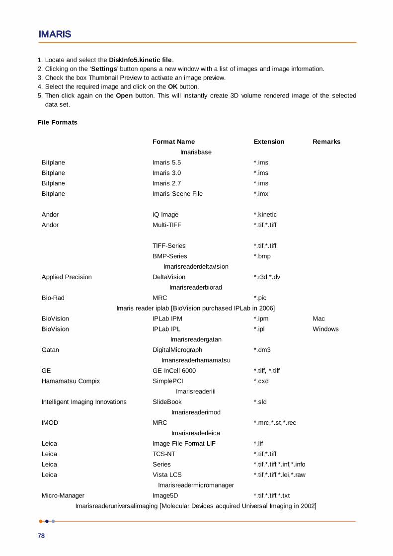
IMARIS

78

1. Locate and select the DiskInfo5.kinetic file.

2. Clicking on the ‘Settings’ button opens a new window with a list of images and image information.



5. Then click again on the Open button. This will instantly create 3D volume rendered image of the selected

data set.

File Formats

Format Name Extension Remarks

Imarisbase




Bitplane Imaris Scene File *.imx

Andor iQ Image *.kinetic

Andor Multi-TIFF *.tif,*.tiff

TIFF-Series *.tif,*.tiff

BMP-Series *.bmp

Imarisreaderdeltavision

Applied Precision DeltaVision *.r3d,*.dv

Imarisreaderbiorad

Bio-Rad MRC *.pic

Imaris reader iplab [BioVision purchased IPLab in 2006]

BioVision IPLab IPM *.ipm Mac

BioVision IPLab IPL *.ipl Windows

Imarisreadergatan

Gatan DigitalMicrograph *.dm3

Imarisreaderhamamatsu

GE GE InCell 6000 *.tiff, *.tiff

Hamamatsu Compix SimplePCI *.cxd

Imarisreaderiii

Intelligent Imaging Innovations SlideBook *.sld

Imarisreaderimod

IMOD MRC *.mrc,*.st,*.rec

Imarisreaderleica

Leica Image File Format LIF *.lif

Leica TCS-NT *.tif,*.tiff

Leica Series *.tif,*.tiff,*.inf,*.info

Leica Vista LCS *.tif,*.tiff,*.lei,*.raw

Imarisreadermicromanager

Micro-Manager Image5D *.tif,*.tiff,*.txt

Imarisreaderuniversalimaging [Molecular Devices acquired Universal Imaging in 2002]

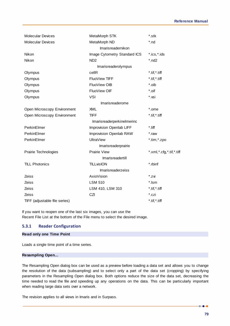
Reference Manual

79

Molecular Devices MetaMorph STK *.stk

Molecular Devices MetaMorph ND *.nd

Imarisreadernikon

Nikon Image Cytometry Standard ICS *.ics,*.ids

Nikon ND2 *.nd2

Imarisreaderolympus

Olympus cellR *.tif,*.tiff

Olympus FluoView TIFF *.tif,*.tiff

Olympus FluoView OIB *.oib

Olympus FluoView OIF *.oif

Olympus VSI *.vsi

Imarisreaderome

Open Microscopy Environment XML *.ome

Open Microscopy Environment TIFF *.tif,*.tiff

Imarisreaderperkinelmerinc

PerkinElmer Improvision Openlab LIFF *.liff

PerkinElmer Improvision Openlab RAW *.raw

PerkinElmer UltraView *.tim,*.zpo

Imarisreaderprairie

Prairie Technologies Prairie View *.xml,*.cfg,*.tif,*.tiff

Imarisreadertill

TILL Photonics TILLvisION *.rbinf

Imarisreaderzeiss

Zeiss AxioVision *.zvi

Zeiss LSM 510 *.lsm

Zeiss LSM 410, LSM 310 *.tif,*.tiff

Zeiss CZI *.czi

TIFF (adjustable file series) *.tif,*.tiff

If you want to reopen one of the last six images, you can use the

Recent File List at the bottom of the File menu to select the desired image.

5.3.1 Reader Configuration

Read only one Time Point

Loads a single time point of a time series.

Resampling Open...

The Resampling Open dialog box can be used as a preview before loading a data set and allows you to change

the resolution of the data (subsampling) and to select only a part of the data set (cropping) by specifying

parameters in the Resampling Open dialog box. Both options reduce the size of the data set, decreasing the

time needed to read the file and speeding up any operations on the data. This can be particularly important

when reading large data sets over a network.

The revision applies to all views in Imaris and in Surpass.

IMARIS

80

Select Imaris Menu - Open or click on the button Open in the Main toolbar.

Click on a file to highlight it and click on the button Resampling File Open ... .

Image Preview

The view on the right side displays as image preview a single time point of the data set. Right-click in the view

and move the mouse pointer to the right to increase brightness. Move the pointer upwards to increase contrast.

Original Size

Display of the original file size.

Subsampling Factor

X,Y,Z, Ch, T

You have the option to specify the Subsampling Factor, i.e., the fraction of data points to be retained. The

subsampling factor can be specified for the x-, y-, z-directions, the channels (Ch), and the time points (T).

Crop Limits (Min/Max)

X, Y, Z, Ch, T, From, To

The Crop Limits (Min/Max) for the x-, y-, z-directions, the channels (Ch), and the time points (T) can also be

specified.

Resampled Size

Display of the resampled file size.

Click on OK and the data set is cropped and resampled while loading.

See also:Menu Edit - Image Properties... - Geometry

Menu Edit - Crop Time...

Menu Edit - Resample Time...

Menu Edit - Crop 3D...

Menu Edit - Resample 3D...

5.3.2 Settings

In the Settings you specify options for reading certain file formats.

Leica LCS Settings

A Leica LCS data set consists of a number of image stacks (or experiments). A dialog box can be opened to

select a specific image stack.

Select File - Open or click Open in the Main toolbar.

Select Files of Type: Leica LCS.

Click on the *.lei file to highlight it and click Settings.

A new window appears with a list of images and image information (Name, Description, Recording Date, Data

Type, Size, Time Points, Channels, Size (MB), voxel size).

By checking the box Thumbnail Preview possibility of activating an image preview is available. The individual

images that belong to that stack will display on the left side.

Reference Manual

81

Select the required image stack on the left side of the dialog box.

Click OK to open the image.

Leica LIF Settings

A Leica LIF data set consists of a number of image stacks (or experiments). A dialog box can be opened to

select a specific image stack.

1. Select File - Open or click Open in the Main toolbar.

2. Select Files of Type: Leica LIF.

3. Click on the *.lif file to highlight it and click Settings. A new window appears with a list of images and image

information (Name, Description, Recording Date, Data Type, Size, Time Points, Channels, Size (MB), voxel

size).

4. By checking the box Thumbnail Preview the possibility of activating an image preview is available. The

individual images that belong to that stack will display on the left side.

5. Select the required image stack on the left side of the dialog box.

6. Click OK to open the image.

Series Reading Sequence

If the data set consists of a series of images, individual images can be sorted according to various dimensions

(i.e. slices, channels, time points, dimension sequence). The reader can handle Tiff series with single and

multiple running numbers.

1. Select the Imaris Menu - the Open option

2. Select Files of Type: Tiff (adjustable file series) and not Tiff (series) from the drop-down list.

3. Select the source folder containing the series.

4. The Settings button only becomes enabled when a TIFF file is selected.

5. In the Series Reading Sequence window you can define the options to combine multiple files into one multi-

dimensional image.

Reference File

Display the full path of the selected file.

Depending on the structure of the file system and the file name extension there are two options you can use:

1. File Names with Delimiter

2. File Names without Delimiter

File names with Delimiter

You can use this option when your files are numbered in sequential order and contain fields of information.

The dialog allows you to specify the order of the dimension within the image series and defines how they should

be arranged in the final sequence. These are Slices: Z, channels: C, time points: T and to split into multiple

datasets/images: F (Split).

You may apply as many or as few dimensions as you wish, depending on your image file requirements.

Assign the appropriate dimension by clicking on the arrow and selecting a dimension from the drop-down

menu.

The selected dimensions are applied to the series of images.

IMARIS

82

Summary

Displays the total number of files selected within the file cluster, as defined by your selection criteria, to be

used to create multi-dimensional image.

The summary number is updated dynamically.

File names without Delimiter

You can use this option when the files are not numbered and contain no separator or delimiter.

The dialog allows you to specify the order of the dimension within the image series and defines how they should

be arranged in the final sequence. If the file is being loaded, the number of dimensions must be specified by the

user so that the algorithm will know when to finish reading the first dimension and continue with the second.

You may apply as many or as few dimensions as you wish, depending on your image file requirements.

Assign the appropriate dimension by clicking on the arrow and select a dimension from the drop-down menu.

Summary

Displays the total number of files selected within the file cluster, as defined by your selection criteria, to be

used to create multi-dimensional image.

The summary number is updated dynamically.

File Arrangement

In the File Arrangement window, the selected sequence and dimension order is shown in tabular form. This

display can be used to validate the sequence parameters.

Validate this information before you apply and open the TIFF series.

F(Split)

The split option F (Split) lets you split a collection of images files into multiple DataSets / Images.

This Settings Dialog is present both in Imaris and in ImarisFileConverter, this option is available in the two

applications:

In ImarisFileConverter, it allows to convert file series into multiple output IMS Files (with the benefit of

configuring the layout and applying the X, Y, Z size)

In Imaris, it allows, to read a single file (or a subset of files) from file series, or load multiple images from

subsets of the series for batch run.

The procedure for how to split a number of files into two ims images, with two channels each is as follows:

In this example there are 4 TIFF files:

- MyTiffFile_f01_c01.tif

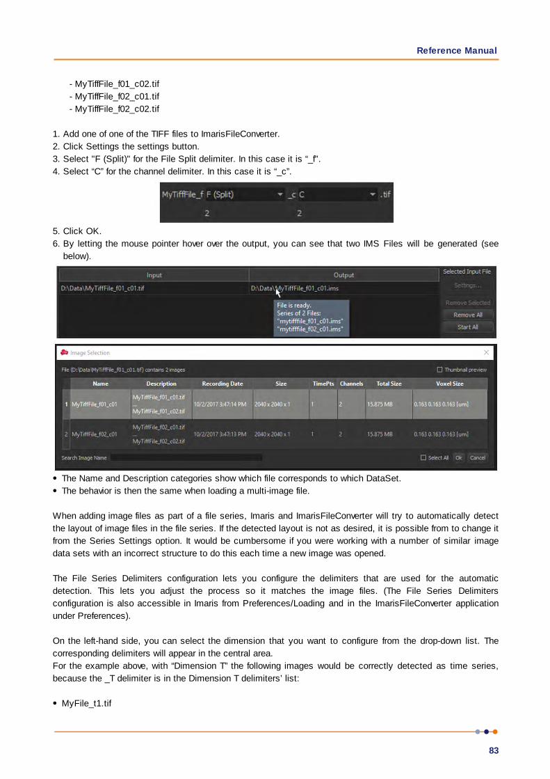
Reference Manual

83




1. Add one of one of the TIFF files to ImarisFileConverter.

2. Click Settings the settings button.

3. Select "F (Split)" for the File Split delimiter. In this case it is “_f".

4. Select “C” for the channel delimiter. In this case it is “_c”.

5. Click OK.

6. By letting the mouse pointer hover over the output, you can see that two IMS Files will be generated (see

below).

The Name and Description categories show which file corresponds to which DataSet.

The behavior is then the same when loading a multi-image file.

When adding image files as part of a file series, Imaris and ImarisFileConverter will try to automatically detect

the layout of image files in the file series. If the detected layout is not as desired, it is possible from to change it

from the Series Settings option. It would be cumbersome if you were working with a number of similar image

data sets with an incorrect structure to do this each time a new image was opened.

The File Series Delimiters configuration lets you configure the delimiters that are used for the automatic

detection. This lets you adjust the process so it matches the image files. (The File Series Delimiters

configuration is also accessible in Imaris from Preferences/Loading and in the ImarisFileConverter application

under Preferences).

On the left-hand side, you can select the dimension that you want to configure from the drop-down list. The

corresponding delimiters will appear in the central area.

For the example above, with “Dimension T” the following images would be correctly detected as time series,

because the _T delimiter is in the Dimension T delimiters’ list:

MyFile_t1.tif

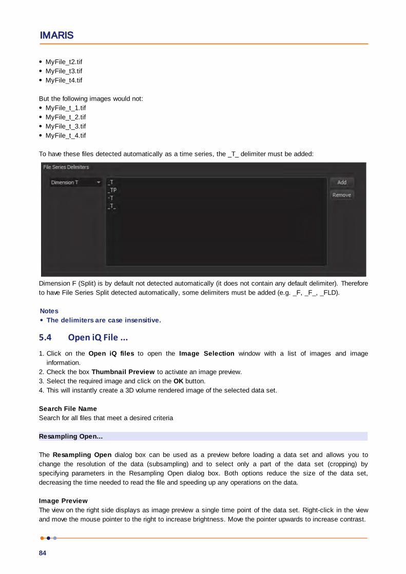
IMARIS

84

MyFile_t2.tif

MyFile_t3.tif

MyFile_t4.tif

But the following images would not:

MyFile_t_1.tif

MyFile_t_2.tif

MyFile_t_3.tif

MyFile_t_4.tif

To have these files detected automatically as a time series, the _T_ delimiter must be added:

Dimension F (Split) is by default not detected automatically (it does not contain any default delimiter). Therefore

to have File Series Split detected automatically, some delimiters must be added (e.g. _F, _F_, _FLD).

Notes

The delimiters are case insensitive.

5.4 Open iQ File ...1. Click on the Open iQ files to open the Image Selection window with a list of images and image

information.



4. This will instantly create a 3D volume rendered image of the selected data set.

Search File Name

Search for all files that meet a desired criteria

Resampling Open...

The Resampling Open dialog box can be used as a preview before loading a data set and allows you to


specifying parameters in the Resampling Open dialog box. Both options reduce the size of the data set,

decreasing the time needed to read the file and speeding up any operations on the data.

Image Preview

The view on the right side displays as image preview a single time point of the data set. Right-click in the view

and move the mouse pointer to the right to increase brightness. Move the pointer upwards to increase contrast.

Reference Manual

85

Original Size

Display of the original file size.

Subsampling Factor

X, Y, Z, Ch, T

You have the option to specify the Subsampling Factor, i.e., the fraction of data points to be retained. The

subsampling factor can be specified for the x-, y-, z-directions, the channels (Ch), and the time points (T).

Crop Limits (Min/Max)

X, Y, Z, Ch, T, From, To

The Crop Limits (Min/Max) for the x-, y-, z-directions, the channels (Ch), and the time points (T) can also be

specified.

Resampled Size

Display of the resampled file size.

Click on OK and the data set is cropped and resampled while loading.

5.5 Store

To save an existing data set click Store in the File menu or Store icon on the Main toolbar.

Selecting this option stores the image data and (any) created objects within the selected Arena Group. The

icon overlaying the image is updated to reflect the newly created surpass objects. The newly created object is

added under Properties in the Surpass tab.

Please note: Store functionality is implemented to be performed at maximum speed. This

functionality overwrites the existing file without warning and only writes changed or new data

without deleting obsolete ones. As a result, the resulting Save file could actually be larger than the

original.

5.6 Store asTo store the changes made to the image in a different file whilst maintaining the original file:

1. Click on the Store as option in the File menu or Store as icon . This option enables you to modify the

image name and creates a new image item within the Arena. The selected group now contains one original

image file which remains unchanged and the new image file with the additionally segmented object. This

newly created image item has an overlaid icon indicating the image type and segmented surpass objects.

Under the Objects tab the newly created object is added.

2. Enter the name for the file to be saved or confirm the suggestion.

3. Select the required file format and click OK.

5.7 Export

To save a newly created Imaris file that contains both image and scene data on your local storage space click

IMARIS

86

on the Export option in the File menu or Export icon .

Saving in Imaris format is recommended whenever the data set is cropped or the parameters changed. Saving adata set in Imaris file format provides the advantage of a faster loading process and the possibility of usingthumbnails. In addition, parameters are saved with the images.

The file extension, suggested as the default, is *.ims. The single created Imaris file contains both the imageand the scene data.

You can save the file when you are done or if you want you can stop in the middle and resume work later.

Simply, choose Export from the File menu and give the file a name you will remember. If you then close the file

and reopen it at a later time, you can resume work from where you left off.

1. In the menu bar select File - Export.... The Save as window displays.

2. Select the directory and enter the name for the file to be saved or confirm the suggestion.

3. Select the requested file format and click OK.

When the work is done, it is recommended to save the data set by using 'Store as'. Selecting the 'Store as'

option could take longer time but will give you the smallest file size possible.

Available File Formats in Imaris



Bitplane: Imaris 2.7 (Classic)(*.ims)

Tiff (series)(*.tif *.tiff)

RGBA-Tiff (series)(*.tif *.tiff)

ICS file (*.ics *.ids)

Olympus: cell^R 1.1/standard (*.tif *.tiff)


Open Microscopy Environment Tiff (*.tif *.tiff)

BMP (series)(*.bmp)

Move file (slice ion) (*.avi, *.mov, *.tif, *.tiff)

5.7.1 Advanced Save Options

Button Format Settings...

A click on the button Format Settings... opens the Imaris Save Options window. See also Open Microscopy

Environment: TIFF and Export as Movie File (Slice Animation).

Window: Save Options


Enable Compression Check the box to use compression.

Export Scene Check the box to save the Imaris scene.


Reference Manual

87

Time Series

Export Single File

The time series are saved in a single file.

Export Multiple Files

For each time point a new file is generated.

Compression

LZW Compression

Check the box to use an LZW compression.

5.7.2 Open Microscopy Environment TIFF Advanced Options

Set the advanced save options when exporting as a Open Microscopy Environment TIFF format by clicking

the Format Settings button. It is possible to set the options for this format from the below:

Dimension order

Select from the following options:

XY ZCT (default)

XT TZC

XT CZT

XY ZTC

XY TCZ

XY CTZ

Number of dimensions on one file

Set the number of dimensions between 2 and 5.

Tiff options

Enable/disable LZW Compression (lossless data compression, default: Off) and set image to be composed of

either Tiles or Strips (default).

5.7.3 Movie File (Slice Animation) Advanced Settings

Set the save options when exporting as a Movie file (Slice Animation) by clicking the Format Settings

button. It is possible to set the options outlined below:

Format

Select from the following file formats:

H264 Movie (default - common high definition format, H.264 compression)

Raw Movie

Tiff (series).tiff

Movie Settings

Adjust the Compression factor between 0 (no compression: best quality/largest file size) and 100 (highest

compression: lowest quality/smallest file size).

Frame rate

IMARIS

88

Set the frame rate for the movie file in frames per second.

5.8 Add Image... (multi-image)New "multi-image" functionality for working with multiple images in a single Imaris scene was introduced in

Imaris 9.1. This feature set may be useful for a range of applications, for example: combining different imaging

modalities on the same sample such as electron microscopy and confocal microscopy, or for images of the

same modality captured at different magnification levels. It is also possible to perform alignment of 3D objects

that were imaged separately.

The features available are described in the following sub-sections along with an overview of how to use these

functions on your images.

The first step is how to add additional images:

How to add your images

1. Open the first image in Surpass view.

2. Load additional images using the Add images... from the File menu.

3. Each additional image can then be seen to have been loaded in the viewing window.

a. When the position tab is selected an XYZ tripod shows the orientation of the selected image.

b. The Align to: box displays an indicator color to help identify the appropriate image.

c. Use the mouse Pointer Navigate mode to navigate through the image area, use the Select mode to

select the required image.

The Settings section describes how the images are displayed and labelled.

If there is more than one image loaded, Imaris will let the user chose which image to perform the required

Reference Manual

89

action on.

Image position adjustment tools are described in section Position.

Note: To remove images, use the Remove images... from the Edit menu, see Remove Images.

Settings Tab Menu Options

Refer to the section tab settings for further information on frame component settings.

Position Tab Menu Options

Align to:

Select the image you want to align the selected image to. The color indicator displayed is representative of the

appropriate image.

Manipulator Anchor

Select the adjustment/rotation point to be either at the Center or the Corner of the image.

Positioning

Use the positioning options to adjust the positioning of image in XY, XZ and YZ planes. The + and - buttons can

be used to adjust in increments. The increment size is set in the Rotation Delta and Translation Delta fields.

The positioning can be fixed about the planes by selecting the Mouse Fixed checkbox for the appropriate

plane. This is useful for locking the movement in the plane/axis as the image is moved.

After making adjustments you can return positioning to the default position or reset to Center using the the

Reset to Default or Reset to Center buttons respectively.

Color Tab Menu Options

Adjust the color settings.

How to Align Images

Alignment can be split into two steps:

Performing the Initial Alignment (Approximate)

1. Add the images as described in Add Image... (multi-image)

IMARIS

90

2. Images can be repositioned in the Select Pointer mode by clicking and holding the left mouse button on the

pink central section and moving to the required location.

3. To change the orientation about the axes, click on the required X, Y or Z axis arms of the tripod and it will

rotate about the selected axis. The plane can be locked in position if required using the Mouse Fixed check

box for the required plane (axis).

4. When aligning images it is useful to turn off unnecessary channels so you may focus on useful image

information to help the alignment. It may also be useful to change the color of the channel you are using for

alignment to one that gives good contrast, making alignment easier.

Above: Image is aligned against the underlying image using the tripod to adjust the relative rotation and translation

about the XY, XZ and YZ planes. Note that channels for both images have been disabled to help visualize the

alignment of the structures during the alignment process.

Performing Precise Alignment

1. Once the images are aligned approximately you may find it useful to switch to a 2D or Slicer view, zooming

in for precise alignment:

2. The plane can be locked in position using the Mouse fixed check box for the required plane (axis).

3. The Rotation and Translation - and + buttons can be used to adjust the position in small increments with a

specific plane until the desired alignment is achieved. The size of these increments can be set in the fields

below. Note that for rotation you can change between having the adjustment in the Center, or the Corner of

the image.

4. This process can be repeated for the other planes and checked until you are happy with the alignment.

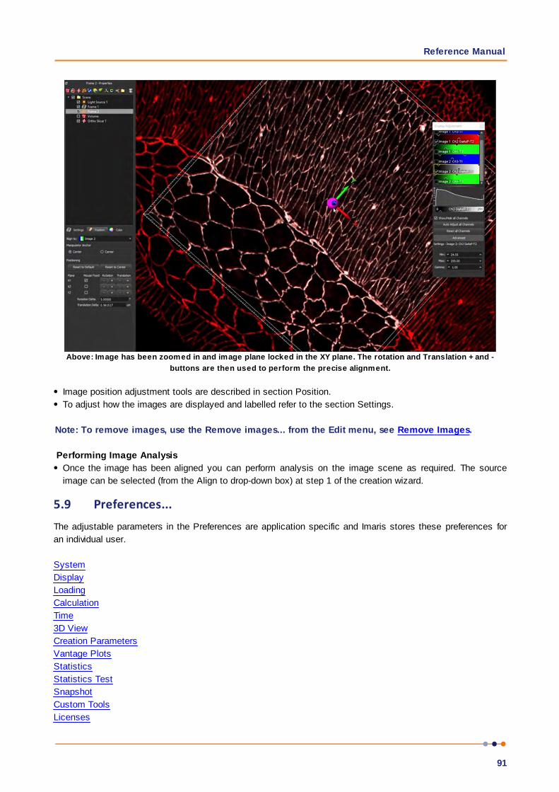
Reference Manual

91

Above: Image has been zoomed in and image plane locked in the XY plane. The rotation and Translation + and -

buttons are then used to perform the precise alignment.

Image position adjustment tools are described in section Position.

To adjust how the images are displayed and labelled refer to the section Settings.

Note: To remove images, use the Remove images... from the Edit menu, see Remove Images.

Performing Image Analysis

Once the image has been aligned you can perform analysis on the image scene as required. The source

image can be selected (from the Align to drop-down box) at step 1 of the creation wizard.

5.9 Preferences...The adjustable parameters in the Preferences are application specific and Imaris stores these preferences for

an individual user.

System

Display

Loading

Calculation

Time

3D View

Creation Parameters

Vantage Plots

Statistics

Statistics Test

Snapshot

Custom Tools

Licenses

IMARIS

92

Update

Usage Data

3D Cursor

Annotate

Arena

Advanced

Imaris Administrator can be accessed directly from Preferences so that licenses, data storage locations and

other Imaris settings can be configured by a user with administrative privileges.

5.9.1 System

Displays the basic system parameters of your computer.

Graphics

OpenGL Renderer

OpenGL Version

Pixel Shader

OpenGL Extensions

Information about the OpenGL Renderer, OpenGL Version, Pixel Shader, and OpenGL Extensions.

Operating System

OS

Version (Build)

Service Pack

Information about the operating system, the installed Version and the service pack.

Memory Status

Physical Memory installed

Physical Memory available

Information about the available amount of internal memory.

Network

Network Interfaces

Information about the available network interfaces

Proxy Settings

Http Proxy Server Name

Enter a proxy server's name. If this field is empty, no proxy server is used.

Http Proxy Server Port

Enter the port to the proxy server. If this field is empty, no proxy server is used.

Test Connection Button

Click on this button to test your proxy settings. If the fields are empty, the connection is tested without using a

proxy server.

Button OK

Reference Manual

93

To apply the changes click on OK.

Button Cancel

If you do not want to save the changes click on Cancel.

5.9.2 Display

Select the viewing properties and the basic colors for the backgrounds and selection in the gallery.

Display

Interpolate

If checked, the images are automatically interpolated for a smoother display.

Texture Cache Limit (MB)

Before displaying any image data, Imaris converts the data into a configuration (called textures) that is

optimized by the graphics hardware. The value of the Texture Cache Limit determines how many textures can

be stored in RAM. The Texture Cache Limit is automatically determined from the available memory of the

graphics board when Imaris is used for the first time. You can also manually set the value to the memory of

your graphics card.

Colors

Background Color

The background color appears when there is no image to be displayed or when the displayed image does not fill

the whole View Area.

Please note: The background color setting has not effect on the MIP mode. The default color for

MIP(max) is black and MIP(min) is white.

Click on the color selection button to open the color selection window to change the respective color.

Background Color 2

Background marking the original position if an image is moved.


Checkered Background for Blending

When using blending mode, a checkered background is displayed in Full 3D blend and in Surpass view.

Tile Size

Allows definition of the tile size for a checkered background.

Linear Color Progress for Blending

The background displays a color gradient in blend progress projections and in Surpass.

Selection Color

Color of selection frame and drawing lines in contour surfaces.


IMARIS

94

Measurement Color

Color of measurements points and lines visible in the image (in the Slice and the 3D view).


User Interface Theme

This option allows you to customize the user interface theme.

You can either choose the Native theme (from OS) or select the Dark theme. Click OK. The display updates

immediately.

Coordinate Axis/Scale TimeColor Bar

Show Coordinates Axis

Show Scale Bar

Show Scale Bar Label

Scale Bar Font Size

Scale Bar Lower Left Corner x

Scale Bar Lower Left Corner y

Show Time Colorbar

Show Date

Show Time

These options change the display of the scale bar, labels and time information in the Slice, Selection, Gallery

and 3D View.

Adjusting the Scale Bar

The scale bar position and size can be set in preferences by adjusting the values in the Scale Bar Font Size,

Scale Bar Lower Left Corner x: and Scale Bar Lower Left Corner y:

You can also alter the length, width, location and font size of the interactive scale bar when the Pointer is in

Select mode. All changes are instantly displayed in the viewing area.

Extend or shorten the scale bar by clicking and dragging one end of it.

Move the scale bar to any location in the viewing by dragging it

Zooming in or out of the image the scale bars are automatically updated.

To choose the style of timestamp to be displayed select either Show Time or Show relative Time.

Show Time option display the acquisition time.

Show relative Time

For Show relative time the first time point is designated as time zero and all other times are displayed relative

to that.

The timestamp presentation format can be chosen and adjusted.

h (hours), min (minutes), s(seconds), f (milliseconds)

Select options to display coordinate axis, date, scale bar, scale bar label or time on screen in the Viewing

Area.

Please note: To display the Coordinates Axis in the Surpass view the option Axis Labels in the

Frame-Tab Setting must be also selected.

Reference Manual

95

Numbers Representation

You can adjust how numbers are represented for the available options:

Unit of Length

Unit of Time

Significant Digits

Off Screen Rendering (for saving Snapshots and Movies)

If deactivated Imaris will take the images similar like a screenshot directly from the display. Uncheck this option

only if you have problems with the Snapshot or Movie export e.g. if the image is distorted. You will not be able

to create an output larger than your physical screen size if this option is disabled.

Show System Monitors

Check this box to display the system monitors in the Status Bar at the bottom of the screen. The first window

displays the "reads per sec", the second the "writes per sec", the third the "write requests in queue" and the

last the "percentage read cache hits". These are useful information especially if you work with huge data sets.

Button OK


Button Cancel


5.9.3 Loading

Allows you to select the color assignment method used when loading data sets and to define the default colors.

Images in Imaris format will display in the colors defined in the image file.

Take Colors from:

Default Colors

Use the default color selection to display the loaded data set. The parameter set Default Colors (see below) is

available.

File Colors (color table or base color if available, otherwise default colors)

Use the original color definition of the loaded data set (usually stored in a lookup table). The parameter set

Default Colors (see below) is not available.

Emission Wavelength (from file if available, otherwise default colors)

Use the color according to the emitted wavelength from the file (corresponds to the appearance under the

microscope). The parameter set Default Colors (see below) is not available.

Please note that not all file formats support lookup tables and emission wavelength.

Default Colors

The parameter set Default Colors is available, if you select Default Colors in the parameter set Take Colors from

(see above).

First Cannel

Second Channel

IMARIS

96

Third Channel

Other Channels

Display of the defined color.

iQ ImageDisk File

1. Either type in the location of the DiskInfo5.kinetic file or use the browse button to find it.

2. Use the Browse button to find and select the DiskInfo5.kinetic file.

3. Open iQ files

4. Clicking on the ‘Open iQ files’ opens the Image Selection window with a list of images and image

information.


6. Select the required image and click on the OK button. This will instantly create a 3D volume rendered image

of the selected data set.

Browse Button

Use the Browse button to find and select the DiskInfo5.kinetic file.

Select... Button

Click on this button to open the color selection window to change the respective color.

OK Button


Button Cancel


5.9.4 Calculation

Calculation

Number of Parallel Jobs

Specify the number of threads (processor cores) used in calculations. See maximum number of available

threads in the System box.

History

Maximum Number of Commands in History

Defines the maximum number of operations that can be undone/redone.

Please note: Each level of image processing requires an additional copy of the full image in

memory. If your machine runs out of memory, set Maximum Number of Commands in History to 1.

Data Cache

Imaris uses a data caching mechanism that allows you to process images that are significantly larger than the

physical memory (RAM) installed in the computer system. This mechanism writes image data blocks to the

disk and reads them back into the physical memory when they are needed.

Memory Limit (MB)

Reference Manual

97

The value of data cache limit controls the amount of data blocks Imaris will keep in memory at any time. Enter

a value based on the following table.

PC & MAC

64 bit Physical memory installed x 0,5

Cache File Paths:

Imaris utilize advanced caching when working with large images. You can add a Cache File Path by defining a

directory where the temporary files should be stored.

Cache File Paths display of the paths to the temporary files (Scratch-disks).

Please note: Setting the Cache File location to a spare or separate hard drive may improve the

performance when working on larger images.

Button Add

Button Remove

You can use the buttons to add or remove file paths in the list.

Button OK


Button Cancel


5.9.5 Time

These are the default parameter settings for the Time Bar.

Play Back

Specify the play back mode for the Time Bar.

Play One Time

All time points of the data set are shown one time. The play back stops when the last time point is reached.

Repeat Forever

Once the play back has reached the last time point, it starts at the first time point again (continuous loop).

Swing Back and Forth Forever

When the last time point is reached, the time sequence is shown in reverse until the first time point is reached.

Frame Rate: ... Frames per Second

You can further specify the frame rate, i.e. the number of frames per second.

Button OK


Button Cancel


IMARIS

98

See also:

Toolbars - Time Bar

5.9.6 3D View

Object Creation Buttons

Check the icons to be displayed on the Objects toolbar in the Surpass View.

Button Move Up

Button Move Down

Highlight an icon and click Move Up or Move Down to define the order of the icons in the Objects toolbar.

Key Frame Animation

Specify the play back mode for the Key Frame Animation.

Play One Time

All time points of the data set are shown one time. The play back stops when the last time point is reached.

Repeat Forever

Once the play back has reached the last time point, it starts at the first time point again (never ending).

Frame Rate ... Frames per Second

You can further specify the frame rate, i.e. the number of frames per second.

Manual tracking auto-connect (Spots and Surfaces)

Delay before auto advancing (s)

You can specify the value between 0.05 and 5 seconds.

Button OK


Button Cancel


Camera

Enable antialiasing (Smooth Lines)

Check the box to display smooth lines.

Enable Draw Style Settings

Check the box to enable the draw options in the Camera Toolbar.

Enable Stereo Camera Settings

Check the box to enable the stereo options in the Camera Toolbar.

Refer to the Camera Toolbar section for further information.

Zoom Point Under Cursor

This option enables zoom to be centered on the point under the Cursor automatically. This may be useful when

you want to zoom to a specific location, for example when using Filament

Reference Manual

99

Autopath and Filament autodepth tracing. This may be disabled for a standard zoom style in which the zoom

will zoom in on the center of the viewing area. Default (On).

Auto Adjust Center Of Rotation

This option enables the rotation point to be centered on the center of the visible part of the image/scene

automatically. When not enabled the image will automatically rotate around the center of the viewing area

window. Default (On).

Zoom Through Data Set

This option provides an auto focus (based on the distance from the camera to the center of the image for zoom

and pan speed and center of rotation) so you may zoom smoothly through an image to the other side. This may

be useful when the point that you want to zoom to is close to the rear of the image. Default (On).

Torch View

Adjust the options for Torch View. You can select between the three following options:

Draw entire dataset (default option)

Draw dataset only around the torch region (full depth)

Draw dataset only around the torch region (local depth)

5.9.7 Creation Parameters

When you save the Creation Parameter file, it is automatically added to the list that is displayed under the Edit/

Preference/Creation Parameters.

The preference window shows a list of all the parameters sets that have been created. To assist you in finding

and organizing the creation parameters, each file is labeled with an object icon, which indicates the type of

creation parameters set.

Click on the name of the creation parameter’s set, the extended window provides an option to view the entire

list of operations, processing instructions and the parameter’s value of the selected set.

Remove Button

This function will remove the selected set of creation parameters from the list.

The Export and Import functions provide an easy way to exchange the creation parameters between different

users or groups.

Export Button

The creation parameters files can be created and exported.

This can be achieved by selecting the creation parameters set from the list and pressing the Export button.

Specify the directory, where you want to save the creation parameter's file, select a name and save it.

Import Button

The creation parameters files, that can be imported, are generated by the Export command.

Specify the directory of the files you want to import and select the file from the chosen location.

IMARIS

100

5.9.8 Vantage Plots

When you save the Vantage Plot file, it is automatically added to the list that is displayed under the Edit/

Preference/Vantage Plots.

The preference window shows a list of all the creation parameters' sets. To assist you in finding and organizing

the creation parameters, each file is labeled with an object icon, which indicates the type of creation

parameters set.

Click on the name of the Vantage Plot, the extended window provides an option to view the entire list of the plot

type, dimensions and the selected statistical variables.

Remove Button

This function will remove the selected Vantage Plot parameters from the list.

The Export and Import functions provide an easy way to exchange the Vantage Plot parameters between

different users or groups.

Export Button

The Vantage Plot parameters files can be created and exported.

This can be achieved by selecting the Vantage Plot parameters set from the list and pressing the Export

button.

Specify the directory, where you want to save the Vantage Plot parameter's file, select a name and save it.

Import Button

The Vantage Plot parameters files, that can be imported, are generated by the Export command.

Specify the directory of the files you want to import and select the file from the chosen location.

5.9.9 Statistics

Imaris features many statistical functions that can be utilised to analyse surpass objects. Statistics are

accessed through the Statistics tab in the surpass view, the options available are specific to each of the

surpass item types e.g. cells or spots. This section provides an introduction to some of the statistical notations

and concepts used in the following statistics topics.

The time indices where the track objects are present are denoted with t ranging from 1 to n.

Descriptions for statistic functions are grouped together for vectors "X, Y, Z" or dimensions "A, B, C". For

example, for Cells - Cell Displacement X, Y, Z there are three individual functions for each component i.e.

Cells - Cell Displacement X, Cells - Cell Displacement Y and Cells - Cell Displacement Z

Three-dimensional vectors are denoted with an arrow:

Length of a vector:

Position of an object at time index:

Reference Manual

101

Time of an object at time index:

Show Statistic Values

Statistics values can be selected (for display, export to MS Excel, or sorting). Check the values to be displayed

when you open the tab Statistics in the Surpass View.

Show All

Check this box and all statistical values are selected. Uncheck the box and all statistical values are

unselected.

For details of the available options please refer to the respective Section:

Menu Edit - Preferences ...

- Statistics

Cell


- Statistics

Filament


- Statistics

Measurement Points


- Statistics

Spots


- Statistics

Surfaces


- Statistics

Volume

Button OK


Button Cancel


See also:

Surpass View - Overview - Properties Area (Tab Statistics)

Coloc - Volume Statistics

5.9.9.1 CellsImarisCell is an Imaris module that performs automated 2D and 3D time-resolved cell image analysis. It

extracts a full spectrum of relevant information, present in the data set, which provides a wide range of options

to analyze 3D and 4D image data. ImarisCell detects some features that are not easily detected by a human

observer, which can lead to the correlation of potential important and otherwise missed variations in the cell

structure and function. Spots statistics can be located in the statistics tab.

Show Statistic Values - Cell

Cells - Cell Acceleration

Acceleration is the change in the Cell velocity over time.

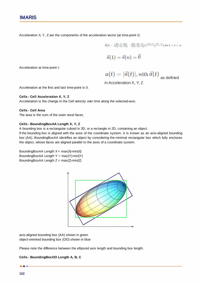
IMARIS

102

Acceleration X, Y, Z are the components of the acceleration vector (at time-point t):

Acceleration at time-point t:

as definedin Acceleration X, Y, Z

Acceleration at the first and last time-point is 0.

Cells - Cell Acceleration X, Y, Z

Acceleration is the change in the Cell velocity over time along the selected-axis.

Cells - Cell Area

The area is the sum of the outer voxel faces.

Cells - BoundingBoxAA Length X, Y, Z

A bounding box is a rectangular cuboid in 3D, or a rectangle in 2D, containing an object.

If the bounding box is aligned with the axes of the coordinate system, it is known as an axis-aligned bounding

box (AA). BoundingBoxAA identifies an object by considering the minimal rectangular box which fully encloses

the object, whose faces are aligned parallel to the axes of a coordinate system.

BoundingBoxAA Length X = max(X)-min(X)

BoundingBoxAA Length Y = max(Y)-min(Y)

BoundingBoxAA Length Z = max(Z)-min(Z)

axis-aligned bounding box (AA) shown in green

object-oriented bounding box (OO) shown in blue

Please note the difference between the ellipsoid axis length and bounding box length.

Cells - BoundingBoxOO Length A, B, C

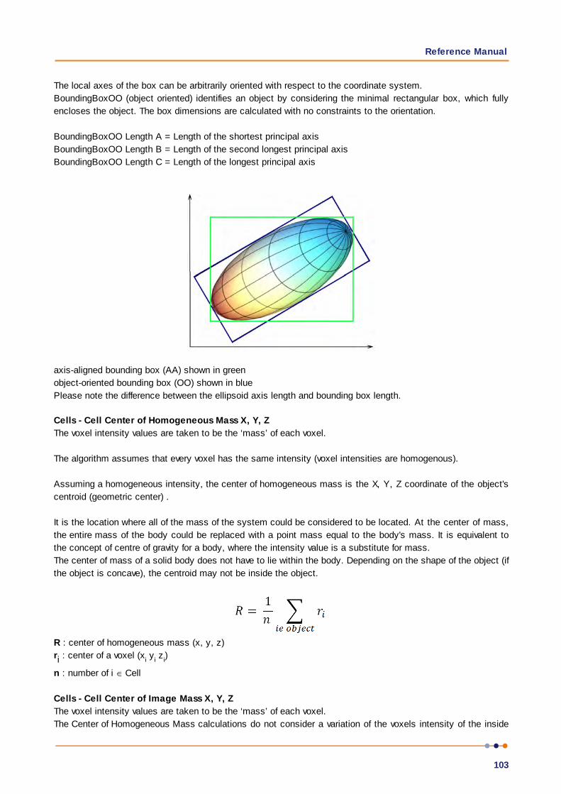
Reference Manual

103

The local axes of the box can be arbitrarily oriented with respect to the coordinate system.

BoundingBoxOO (object oriented) identifies an object by considering the minimal rectangular box, which fully

encloses the object. The box dimensions are calculated with no constraints to the orientation.

BoundingBoxOO Length A = Length of the shortest principal axis

BoundingBoxOO Length B = Length of the second longest principal axis

BoundingBoxOO Length C = Length of the longest principal axis




Cells - Cell Center of Homogeneous Mass X, Y, Z

The voxel intensity values are taken to be the ‘mass’ of each voxel.

The algorithm assumes that every voxel has the same intensity (voxel intensities are homogenous).

Assuming a homogeneous intensity, the center of homogeneous mass is the X, Y, Z coordinate of the object's

centroid (geometric center) .

It is the location where all of the mass of the system could be considered to be located. At the center of mass,

the entire mass of the body could be replaced with a point mass equal to the body's mass. It is equivalent to

the concept of centre of gravity for a body, where the intensity value is a substitute for mass.

The center of mass of a solid body does not have to lie within the body. Depending on the shape of the object (if

the object is concave), the centroid may not be inside the object.

R : center of homogeneous mass (x, y, z)

ri : center of a voxel (xi y

i z

i)

n : number of i Cell

Cells - Cell Center of Image Mass X, Y, Z


The Center of Homogeneous Mass calculations do not consider a variation of the voxels intensity of the inside

IMARIS

104

the object. In the case of an inhomogeneous distribution of the voxel intensity inside the objects, intensity-

based measure may be needed.

The center of mass is calculated using a contribution of each channel and each voxel of the object, based on

each voxel intensity value.

Its positions depend on respective intensities of each voxel in the volume.

The Center of Image Mass is the object centroid calculated by taking into account the voxel intensities of each

channel separately.

The X, Y and Z are coordinates of the intensity-weighted centroid of the object.

R : center of image mass (x, y, z)

mi : voxel intensity


i z

i)

M : sum of voxel intensities

Cells - Cell Cytoplasm Area

Measure the area of the cytoplasm within the Cell. It is calculated as sum of Cell area and Nucleus area.

Cells - Cell Cytoplasm Vesicle Diameter Max

The maximum diameter of all Vesicles within the Cell cytoplasm.The value is separately calculated for each

vesicle type.

Cells - Cell Cytoplasm Vesicle Diameter Mean

The mean diameter of all Vesicles within the Cell cytoplasm.The value is separately calculated for each vesicle

type.

Cells - Cell Cytoplasm Vesicle Diameter Min

The minimum diameter of all Vesicles within the Cell cytoplasm. The value is separately calculated for each

vesicle type.

Cells - Cell Cytoplasm Intensity Max

Cells - Cell Cytoplasm Intensity Mean

Cells - Cell Cytoplasm Intensity Min

Cells - Cell Cytoplasm Intensity StdDev

Cells - Cell Cytoplasm Intensity Sum

The voxel intensity statistics describe the voxels enclosed within the Cytoplasm (Center, Max, Mean, Min,

StdDev and Sum).

Cells - Cell Cytoplasm Number of Vesicles

The total number of Vesicles objects within the cytoplasm. The value is separately calculated for each vesicle

type.

Cells - Cell Cytoplasm Number of Voxels

The total number of voxels within the cytoplasm.

Cells - Cell Cytoplasm Volume

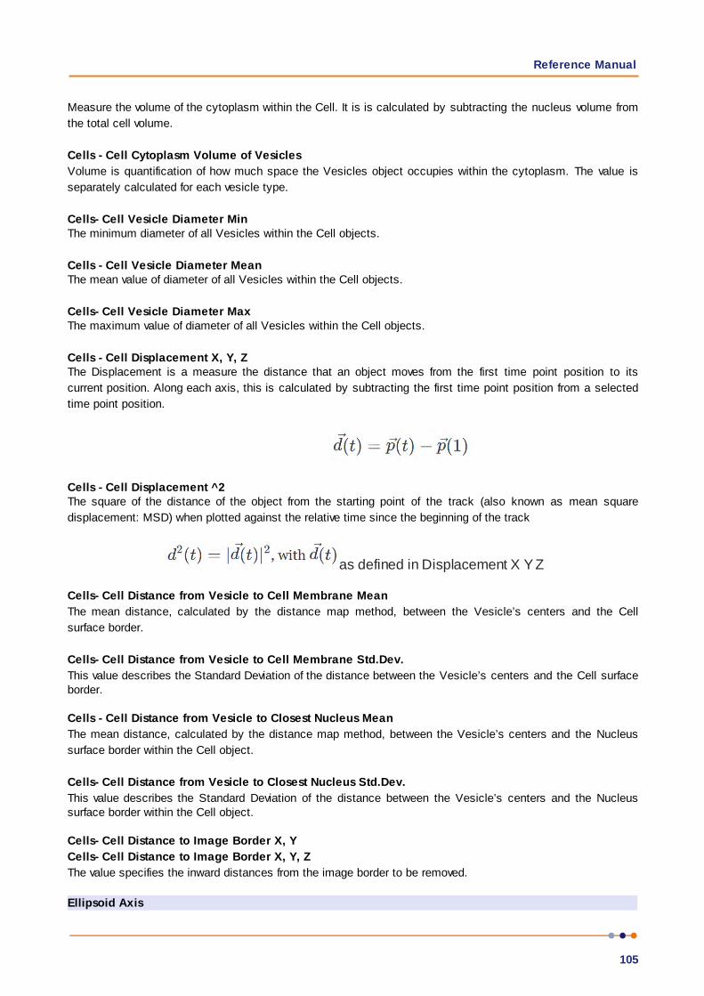
Reference Manual

105

Measure the volume of the cytoplasm within the Cell. It is is calculated by subtracting the nucleus volume from

the total cell volume.

Cells - Cell Cytoplasm Volume of Vesicles

Volume is quantification of how much space the Vesicles object occupies within the cytoplasm. The value is

separately calculated for each vesicle type.

Cells- Cell Vesicle Diameter Min The minimum diameter of all Vesicles within the Cell objects.

Cells - Cell Vesicle Diameter MeanThe mean value of diameter of all Vesicles within the Cell objects.

Cells- Cell Vesicle Diameter Max The maximum value of diameter of all Vesicles within the Cell objects.

Cells - Cell Displacement X, Y, ZThe Displacement is a measure the distance that an object moves from the first time point position to its

current position. Along each axis, this is calculated by subtracting the first time point position from a selected

time point position.

Cells - Cell Displacement ^2The square of the distance of the object from the starting point of the track (also known as mean square

displacement: MSD) when plotted against the relative time since the beginning of the track

as defined in Displacement X Y Z

Cells- Cell Distance from Vesicle to Cell Membrane Mean

The mean distance, calculated by the distance map method, between the Vesicle’s centers and the Cell

surface border.

Cells- Cell Distance from Vesicle to Cell Membrane Std.Dev.

This value describes the Standard Deviation of the distance between the Vesicle’s centers and the Cell surfaceborder.

Cells - Cell Distance from Vesicle to Closest Nucleus Mean

The mean distance, calculated by the distance map method, between the Vesicle’s centers and the Nucleus

surface border within the Cell object.

Cells- Cell Distance from Vesicle to Closest Nucleus Std.Dev.

This value describes the Standard Deviation of the distance between the Vesicle’s centers and the Nucleussurface border within the Cell object.

Cells- Cell Distance to Image Border X, Y

Cells- Cell Distance to Image Border X, Y, Z

The value specifies the inward distances from the image border to be removed.

Ellipsoid Axis

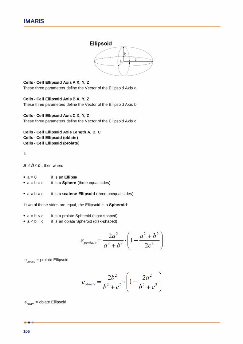
IMARIS

106

Cells - Cell Ellipsoid Axis A X, Y, Z

These three parameters define the Vector of the Ellipsoid Axis a.

Cells - Cell Ellipsoid Axis B X, Y, Z

These three parameters define the Vector of the Ellipsoid Axis b.

Cells - Cell Ellipsoid Axis C X, Y, Z

These three parameters define the Vector of the Ellipsoid Axis c.

Cells - Cell Ellipsoid Axis Length A, B, C

Cells - Cell Ellipsoid (oblate)

Cells - Cell Ellipsoid (prolate)

If:

a b c , then when:

a = 0 it is an Ellipse

a = b = c it is a Sphere (three equal sides)

a b c it is a scalene Ellipsoid (three unequal sides)

If two of these sides are equal, the Ellipsoid is a Spheroid:

a = b < c it is a prolate Spheroid (cigar-shaped)

a < b = c it is an oblate Spheroid (disk-shaped)

eprolate

= prolate Ellipsoid

eoblate

= oblate Ellipsoid

Reference Manual

107

Cells - Cell Intensity Center

Cells - Cell Intensity Max

Cells - Cell Intensity Mean

Cells - Cell Intensity Median

The Cells - intensity median is estimated from the intensity histogram.

Cells - Cell Intensity Min

Cells - Cell Intensity StdDev

Cells - Cell Intensity Sum

The voxel intensity statistics describe the voxels enclosed within the Cell (Center, Max, Mean, Median, Min,

StdDev and Sum).

Cells - Cell Intensity Min of Vesicles

This value describes the minimum voxel intensity of the Vesicles within the Cell object.

Cells - Cell Intensity Max of Vesicles

This value describes the maximum voxel intensity of the Vesicles within the Cell object.

Cells - Cell Intensity mean of Vesicles

This value describes the mean voxel intensity of the Vesicles within the Cell object.

Cells - Cell Nucleus to Cytoplasm Volume Ratio

The value is defined as the ratio between Nucleus volume and Cell cytoplasm volume. The Cell cytoplasm

volume is calculated by subtracting the volume of the Nuclei from the whole cell object volume.

Cells - Cell Number of Nucleus

The number of the Nucleus objects within the selected Cell object.

Cells - Cell Number of Vesicles

The number of the Vesicle objects within the selected Cell object.

Cells- Cell Number of Tracks

This value describes the total number of the Cell's object tracks.

Cells - Cell Number of Voxels

Number of voxels within the selected Cell.

Cells - Cell Position X, Y, Z

Defines the value of X, Y, Z Cell position (x y z).It is equal to Center of Homogeneous Mass of the object

Cells - Cell Relative Vesicle Position Min

Cells - Cell Relative Vesicle Position Mean

Cells - Cell Relative Vesicle Position Max

This parameter provides Min Max and Mean values of all Vesicle Relative Positions within the cell object. This

value describes the Vesicle position within the cell relative to the Nucleus and Cell object’s borders.

Vesicle Relative positions is the ratio between Vesicle distance from the Nucleus border and the sum of

Vesicle’s distances from the Nucleus and Cell border.

If the Vesicle is located within the Nucleus the value is set to 0. If the value is 1 then the Vesicle is located at

the border of Cell object.

Cells - Cell Speed

The Cell speed is the instantaneous speed of the object (um/s).

The instantaneous speed is the scalar equivalent of the object velocity.

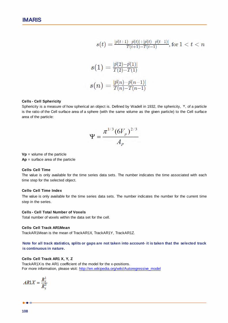
IMARIS

108

Cells - Cell Sphericity

Sphericity is a measure of how spherical an object is. Defined by Wadell in 1932, the sphericity, , of a particle

is the ratio of the Cell surface area of a sphere (with the same volume as the given particle) to the Cell surface

area of the particle:

Vp = volume of the particle

Ap = surface area of the particle

Cells- Cell Time

The value is only available for the time series data sets. The number indicates the time associated with each

time step for the selected object.

Cells- Cell Time Index

The value is only available for the time series data sets. The number indicates the number for the current time

step in the series.

Cells - Cell Total Number of Voxels

Total number of voxels within the data set for the cell.

Cells- Cell Track AR1Mean

TrackAR1Mean is the mean of TrackAR1X, TrackAR1Y, TrackAR1Z.

Note for all track statistics, splits or gaps are not taken into account- it is taken that the selected track

is continuous in nature.

Cells- Cell Track AR1 X, Y, Z

TrackAR1X is the AR1 coefficient of the model for the x-positions. For more information, please visit: http://en.wikipedia.org/wiki/Autoregressive_model

http://en.wikipedia.org/wiki/Autoregressive_model

Reference Manual

109

AR1X = TrackAR1X

tL = last time index of track

tF = first time index of track

Dx(t F,t L) = Px(t L) - Px(t F)

PX(t) = x-position of object at time index t



Cells-Cell Track Area Mean

The mean of the triangle Cell object surfaces along the track.

Cells - Cell Track Center of Homogeneous Mass X, Y, Z












i z

i)

n : number of i Surfaces

Cells - Cell Track Center of Image Mass X, Y, Z


IMARIS

110








channel separately.





i z

i)


Cells - Cell Track Cytoplasm Intensity MaxThis value describes the maximum voxel intensity of the Cytoplasm along the tracks.

Cells - Cell Track Cytoplasm Intensity MeanThis value describes the mean voxel intensity of the Cytoplasm along the tracks.

Cells - Cell Track Cytoplasm Intensity MinThis is the minimum value of all minimum (voxel) intensities of the cells along the tracks

Cells - Cell Track Cytoplasm Intensity SumThis value describes the sum of voxel intensity of the Cytoplasm along the tracks.

Cells - Cell Track Cytoplasm Number of Vesicles MeanThe mean number of Vesicle objects along the track within the Cytoplasm.

Cells - Cell Track Displacement LengthThe Track Displacement Length is the distance between the first and last Cell's position.

defined in Track Displacement X, Y, Z

Cells - Cell Track Displacement X, Y, Z

The object’s Track Displacement is the distance between the first and last object’s position along the selected-

axis.

Cells - Cell Displacement Delta XYZ

The difference in position of the current object and the previous object of the same track.

Reference Manual

111

Cells - Cell Displacement Delta Length (a scalar value)

The length of the position difference of the current object and the previous object of the same track.

Cells - Cell Track Duration

The Track Duration is the duration between the first and last time point within the track.

Cells - Cell Track Ellipsoid Axis A X, Y, Z Mean

These three parameters define the Vector of the track Ellipsoid Axis a.

Cells - Cell Track Ellipsoid Axis B X, Y, Z Mean

These three parameters define the Vector of the track Ellipsoid Axis b.

Cells - Cell Track Ellipsoid Axis C X, Y, Z Mean

These three parameters define the Vector of the track Ellipsoid Axis c.

Cells - Cell Track Ellipsoid Axis Length A, B, C Mean

These three parameters define the length of the Ellipsoid Axis a, b, and c.

Cells - Cell Track Ellipsoid Oblate A Mean

This parameter defines the mean Ellipsoid Oblate for the track (see above for the detailed oblate definition).

Cells - Cell Track Ellipsoid Prolate A Mean

This parameter defines the mean Ellipsoid Prolate for the track (see above for the detailed prolate definition).

Cells - Cell Track Intensity Center Mean

This value describes the mean voxel intensity in the center of the Cell along the tracks.

Cells - Cell Track Intensity Max

This is the maximum value of all maximum (voxel) intensities of the Cell along the tracks

Cells - Cell Track Intensity Mean

This is the weighted mean of the objects means, equal to the simple mean of all the intensities of all theobjects in a track. Larger objects have a larger impact on the track mean.

Cells - Cell Track Intensity Median

The median intensity for a track is calculated as the (approximated) median of the (approximated) medians of

its objects, instead of the true median of all the intensities in the track, for performance reasons.

Cells - Cell Track Intensity Min

This is the minimum value of all minimum (voxel) intensities of the Cell along the tracks.

Cells - Cell Track Intensity StdDev

This value describes the Standard Deviation voxel intensity of the Cell along the tracks.

Cells - Cell Track Intensity Sum

This value is the sum of all sum (voxel) intensities of the Cell along the tracks.

Cells - Cell Track Length

IMARIS

112

The Track Length is the total length of displacements within the track.

Note for all track statistics, splits or gaps are not taken into account- it is taken that the selected tack


Cells- Cell Track Number of Nuclei Mean

The mean number of Nuclei objects along the track.

Cells-Cell Track Number of Vesicle Mean

The mean number of Vesicle objects along the track.

Cells - VesicleTrack Number of Branches

The number of branches along the track.

Cells - Vesicle Track Number of Fusions

The number of fusions along the track.

Cells - Cell Tracks Position Mean X, Y, Z

Defines the mean value of X, Y, Z track positions.

Cells - Cell Tracks Position X, Y, Z Start

Defines the value of the X, Y, Z track start positions.

Cells - Cell Track Speed Max

The maximum value of the object’s speed on the track.

Cells - Cell Track Speed Mean

The Average value of the object’s speed on the track. If the Track has no Fuse (merge) or Fragments (splits),

then the average speed is given by the Track length divided by the time between first and last object in the

Track.

Cells - Cell Track Speed Min

The minimum value of the object’s speed on the track.

Cells - Cell Track Speed Standard Deviation

The Standard Deviation value of the object’s speed on the track.

Cells - Cell Track Speed Variation

The Track Speed Variation is defined as the ratio of the Track Standard Deviation to the Track Speed Mean

value.The coefficient of variation is a dimensionless number.

- Standard Deviation-Mean value

Cells-Cell Track Sphericity Mean

Reference Manual

113

Describes the mean Cell object Sphericity along the tracks.

Cells - Cell Track Straightness

S = TrackStraightness

D = TrackDisplacement

L = TrackLength

Cells - Cell Track Volume Mean

The mean volume of all Cell objects along the tracks.

Note for all track statistics splits or gaps are not taken into account- it is taken that the selected track


Cells - Cell Velocity X, Y, Z

The formulas for calculating the velocity at time points (t) and (1) are calculated as follows:

Cells - Cell Volume

Volume is quantification of how much space a Cell object occupies.

Cells - Cell Volume of Vesicles

Volume is quantification of how much space the Vesicles object occupies within the Cell.

Cells- Nucleus Acceleration

Acceleration is the change in the Nucleus velocity over time.



as defined in Acceleration X, Y, Z


Cells - Nucleus Acceleration X, Y, Z

Acceleration is the change in the Nucleus velocity over time along the selected-axis.

IMARIS

114

Cells - Nucleus Area

The area is the sum of the outer Nucleus voxel faces.

Cells - Nucleus BoundingBoxAA Length X, Y, Z











Cells - Nucleus BoundingBoxOO Length A, B, C







Reference Manual

115




Cells - Nucleus Center of Homogeneous Mass X, Y, Z












i z

i)

n : number of i Nucleus

Cells - Nucleus Center of Image Mass X, Y, Z








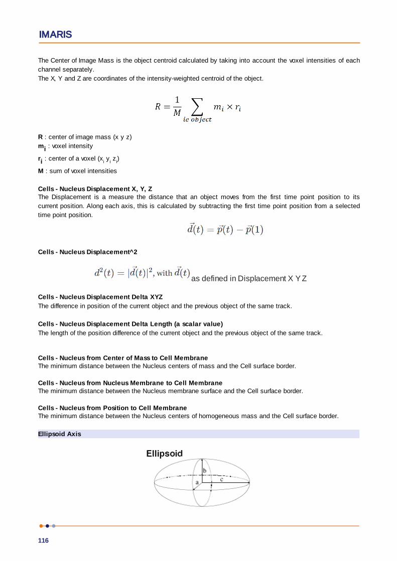
IMARIS

116


channel separately.


R : center of image mass (x y z)



i z

i)


Cells - Nucleus Displacement X, Y, ZThe Displacement is a measure the distance that an object moves from the first time point position to its



Cells - Nucleus Displacement^2


Cells - Nucleus Displacement Delta XYZ


Cells - Nucleus Displacement Delta Length (a scalar value)


Cells - Nucleus from Center of Mass to Cell MembraneThe minimum distance between the Nucleus centers of mass and the Cell surface border.

Cells - Nucleus from Nucleus Membrane to Cell MembraneThe minimum distance between the Nucleus membrane surface and the Cell surface border.

Cells - Nucleus from Position to Cell MembraneThe minimum distance between the Nucleus centers of homogeneous mass and the Cell surface border.

Ellipsoid Axis

Reference Manual

117

Cells - Nucleus Ellipsoid Axis A X, Y, Z

These three parameters define the Vector of the Ellipsoid Axis a.

Cells - Nucleus Ellipsoid Axis B X, Y, Z

These three parameters define the Vector of the Ellipsoid Axis b.

Cells - Nucleus Ellipsoid Axis C X, Y, Z

These three parameters define the Vector of the Ellipsoid Axis c.

Cells - Nucleus Ellipsoid Axis Length A, B, C

Cells - Nucleus Ellipsoid (oblate)

Cells - Nucleus Ellipsoid (prolate)

If we assume a b c , then when:







eprolate

= prolate Ellipsoid

eoblate

= oblate Ellipsoid

Cells - Nucleus Intensity Center

Cells - Nucleus Intensity Max

Cells - Nucleus Intensity Mean

Cells - Nucleus Intensity Median

The Cells - Nucleus intensity median is estimated from the intensity histogram.

Cells - Nucleus Intensity Min

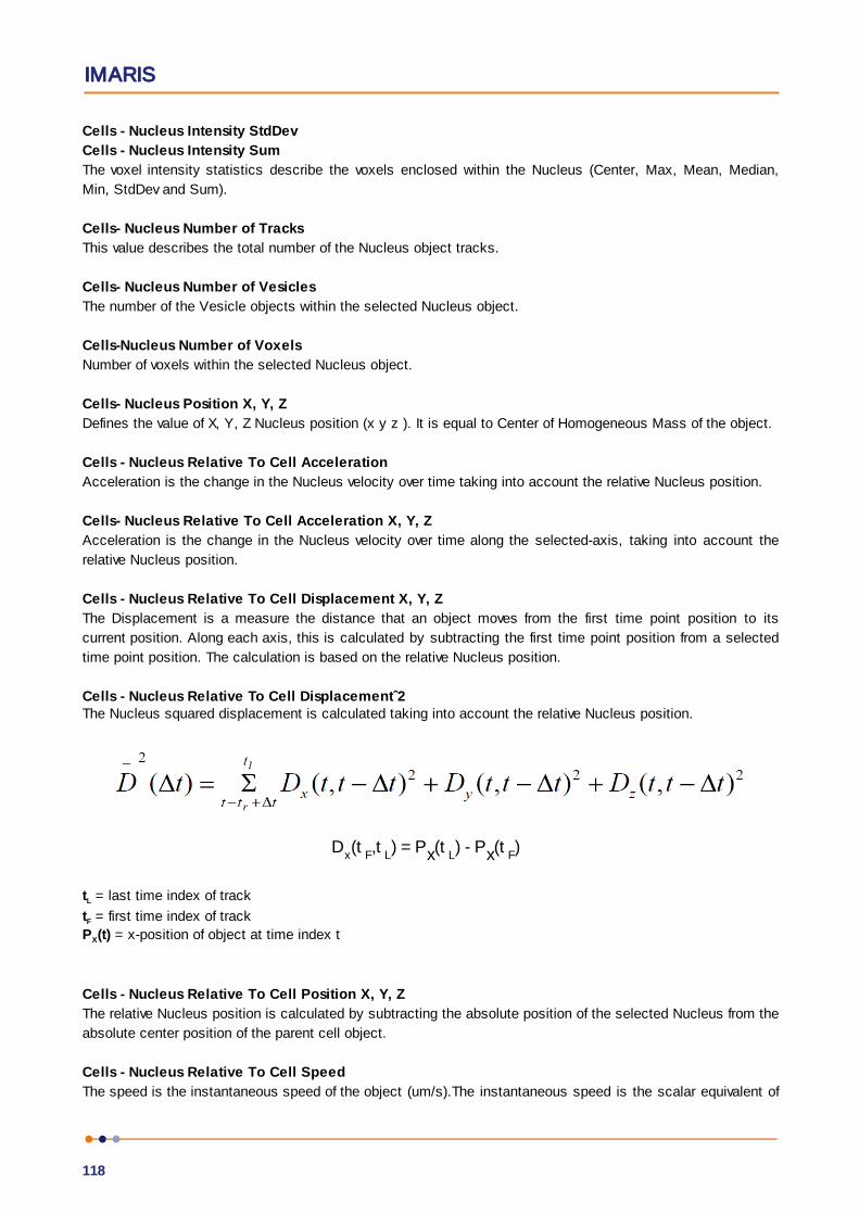
IMARIS

118

Cells - Nucleus Intensity StdDev

Cells - Nucleus Intensity Sum

The voxel intensity statistics describe the voxels enclosed within the Nucleus (Center, Max, Mean, Median,

Min, StdDev and Sum).

Cells- Nucleus Number of Tracks

This value describes the total number of the Nucleus object tracks.

Cells- Nucleus Number of Vesicles

The number of the Vesicle objects within the selected Nucleus object.

Cells-Nucleus Number of Voxels

Number of voxels within the selected Nucleus object.

Cells- Nucleus Position X, Y, Z

Defines the value of X, Y, Z Nucleus position (x y z ). It is equal to Center of Homogeneous Mass of the object.

Cells - Nucleus Relative To Cell Acceleration

Acceleration is the change in the Nucleus velocity over time taking into account the relative Nucleus position.

Cells- Nucleus Relative To Cell Acceleration X, Y, Z

Acceleration is the change in the Nucleus velocity over time along the selected-axis, taking into account the

relative Nucleus position.

Cells - Nucleus Relative To Cell Displacement X, Y, Z

The Displacement is a measure the distance that an object moves from the first time point position to its


time point position. The calculation is based on the relative Nucleus position.

Cells - Nucleus Relative To Cell Displacementˆ2The Nucleus squared displacement is calculated taking into account the relative Nucleus position.

Dx(t

F,t

L) = Px(t

L) - Px(t

F)




Cells - Nucleus Relative To Cell Position X, Y, Z

The relative Nucleus position is calculated by subtracting the absolute position of the selected Nucleus from the

absolute center position of the parent cell object.

Cells - Nucleus Relative To Cell Speed

The speed is the instantaneous speed of the object (um/s).The instantaneous speed is the scalar equivalent of

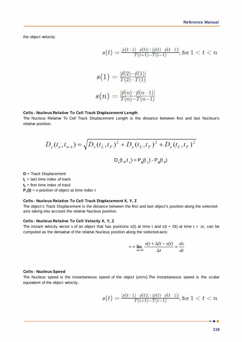
Reference Manual

119

the object velocity.

Cells - Nucleus Relative To Cell Track Displacement Length

The Nucleus Relative To Cell Track Displacement Length is the distance between first and last Nucleus's

relative position.

Dx(t

F,t

L) = Px(t

L) - Px(t

F)

D = Track Displacement




Cells - Nucleus Relative To Cell Track Displacement X, Y, Z

The object’s Track Displacement is the distance between the first and last object’s position along the selected-axis taking into account the relative Nucleus position.

Cells - Nucleus Relative To Cell Velocity X, Y, Z

The instant velocity vector v of an object that has positions x(t) at time t and x(t + Dt) at time t + t, can be

computed as the derivative of the relative Nucleus position along the selected-axis:

Cells - Nucleus Speed

The Nucleus speed is the instantaneous speed of the object (um/s).The instantaneous speed is the scalar

equivalent of the object velocity.

IMARIS

120

Cells - Nucleus Sphericity

Sphericity is a measure of how spherical an object is. Defined by Wadell in 1932, the sphericity, , of a particle

is the ratio of the Nucleus surface area of a sphere (with the same volume as the given particle) to the Cell

surface area of the particle:



Cells - Nucleus Time



Cells - Nucleus Time Index


step in the series.

Cells - Nucleus Total Number of Voxels

Total number of voxels of the Nucleus voxels within the data set.

Cells - Nucleus Track AR1Mean


Cells - Nucleus Track AR1 X, Y, Z


AR1X = TrackAR1X



Dx(t 2,t1) = Px(t2) - Px(t1)


Reference Manual

121




Cells - Nucleus Track Area Mean

The mean of the triangle Nucleus object surfaces along the track.

Cells - Nucleus Track Center of Homogeneous Mass X, Y, Z










R : center of homogeneous mass (x y z)


i z

i)

n : number of i Nucleus

Cells - Nucleus Track Center of Image Mass X, Y, Z









channel separately.


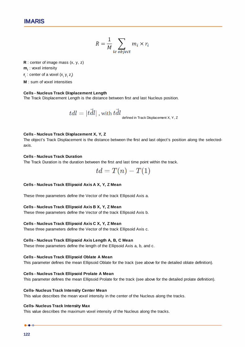
IMARIS

122



ri : center of a voxel (x

i y

i z

i)


Cells - Nucleus Track Displacement LengthThe Track Displacement Length is the distance between first and last Nucleus position.


Cells - Nucleus Track Displacement X, Y, Z


axis.

Cells - Nucleus Track Duration


Cells - Nucleus Track Ellipsoid Axis A X, Y, Z Mean

These three parameters define the Vector of the track Ellipsoid Axis a.

Cells - Nucleus Track Ellipsoid Axis B X, Y, Z Mean

These three parameters define the Vector of the track Ellipsoid Axis b.

Cells - Nucleus Track Ellipsoid Axis C X, Y, Z Mean

These three parameters define the Vector of the track Ellipsoid Axis c.

Cells - Nucleus Track Ellipsoid Axis Length A, B, C Mean

These three parameters define the length of the Ellipsoid Axis a, b, and c.

Cells - Nucleus Track Ellipsoid Oblate A Mean

This parameter defines the mean Ellipsoid Oblate for the track (see above for the detailed oblate definition).

Cells - Nucleus Track Ellipsoid Prolate A Mean

This parameter defines the mean Ellipsoid Prolate for the track (see above for the detailed prolate definition).

Cells- Nucleus Track Intensity Center Mean

This value describes the mean voxel intensity in the center of the Nucleus along the tracks.

Cells- Nucleus Track Intensity Max

This value describes the maximum voxel intensity of the Nucleus along the tracks.

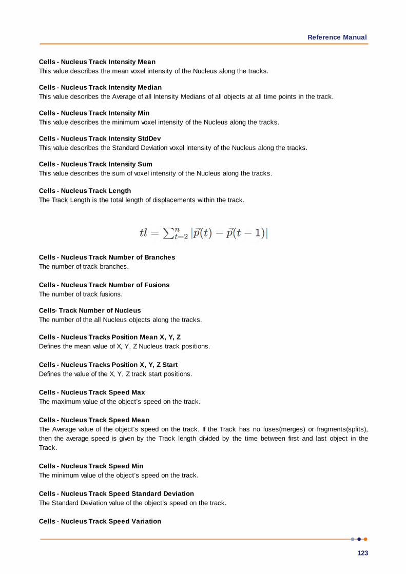
Reference Manual

123

Cells - Nucleus Track Intensity Mean

This value describes the mean voxel intensity of the Nucleus along the tracks.

Cells - Nucleus Track Intensity Median

This value describes the Average of all Intensity Medians of all objects at all time points in the track.

Cells - Nucleus Track Intensity Min

This value describes the minimum voxel intensity of the Nucleus along the tracks.

Cells - Nucleus Track Intensity StdDev

This value describes the Standard Deviation voxel intensity of the Nucleus along the tracks.

Cells - Nucleus Track Intensity Sum

This value describes the sum of voxel intensity of the Nucleus along the tracks.

Cells - Nucleus Track Length


Cells - Nucleus Track Number of Branches

The number of track branches.

Cells - Nucleus Track Number of Fusions

The number of track fusions.

Cells- Track Number of Nucleus

The number of the all Nucleus objects along the tracks.

Cells - Nucleus Tracks Position Mean X, Y, Z

Defines the mean value of X, Y, Z Nucleus track positions.

Cells - Nucleus Tracks Position X, Y, Z Start


Cells - Nucleus Track Speed Max


Cells - Nucleus Track Speed Mean

The Average value of the object’s speed on the track. If the Track has no fuses(merges) or fragments(splits),


Track.

Cells - Nucleus Track Speed Min


Cells - Nucleus Track Speed Standard Deviation


Cells - Nucleus Track Speed Variation

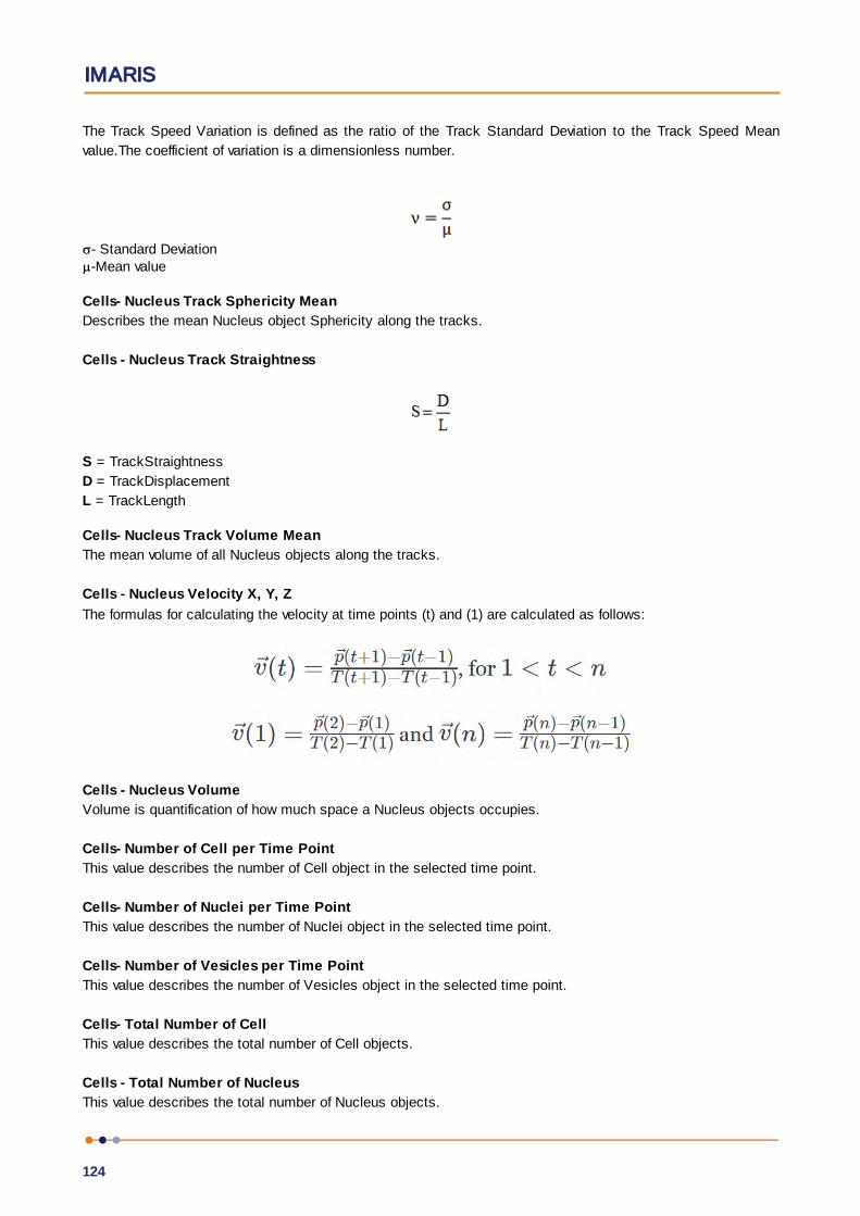
IMARIS

124




Cells- Nucleus Track Sphericity Mean

Describes the mean Nucleus object Sphericity along the tracks.

Cells - Nucleus Track Straightness



L = TrackLength

Cells- Nucleus Track Volume Mean

The mean volume of all Nucleus objects along the tracks.

Cells - Nucleus Velocity X, Y, Z


Cells - Nucleus Volume

Volume is quantification of how much space a Nucleus objects occupies.

Cells- Number of Cell per Time Point

This value describes the number of Cell object in the selected time point.

Cells- Number of Nuclei per Time Point

This value describes the number of Nuclei object in the selected time point.

Cells- Number of Vesicles per Time Point

This value describes the number of Vesicles object in the selected time point.

Cells- Total Number of Cell

This value describes the total number of Cell objects.

Cells - Total Number of Nucleus

This value describes the total number of Nucleus objects.

Reference Manual

125

Cells - Total Number of Vesicles

This value describes the total number of Vesicles objects.

Cells- Cell Track Number of Cells

The number of the all Cell objects along the tracks.

Cells- Track Number of Nuclei

The number of the all Nucleus objects along the tracks.

Cells- Track Number of Vesicles

The number of the all Vesicles objects along the tracks.

Cells - Vesicle Acceleration

Acceleration is the change in the Vesicle velocity over time.




Cells - Vesicle Acceleration X, Y, Z

Acceleration is the change in the Vesicle velocity over time along the selected-axis.

Cells- Vesicle Area

The area is the sum of the outer Vesicles voxel faces.

Cells- Vesicle Diameter X, Y, Z

This value describes the Vesicle diameter along the selected-axis.

Cells - Vesicles Displacement X, Y, ZThe Displacement is a measure the distance that an object moves from the first time point position to its



Cells - Vesicles Displacement^2


Cells - Vesicles Displacement Delta XYZ

IMARIS

126


Cells - Vesicles Displacement Delta Length (a scalar value)


Cells- Vesicle Distance to Cell Membrane

The distance, calculated by the distance map method, between the selected Vesicle centers and the Cell

surface border.

Cells- Vesicle Distance to Closest Nucleus

The distance, calculated by the distance map method, between the selected Vesicle center and the closest

Nucleus surface border. For Vesicles located inside a Nucleus, this distance is a negative number.

Cells- Vesicle Distance to Closest Nucleus Center

The distance between the selected Vesicle center and the center of the closest Nucleus. For Vesicles located

inside a Nucleus, this distance is a negative number.

Cells- Vesicle Intensity Center

Cells- Vesicle Intensity Max

Cells- Vesicle Intensity Mean

Cells- Vesicle Intensity Median

The Cells- vesicle intensity median is estimated from the intensity histogram.

Cells- Vesicle Intensity Min

Cells- Vesicle Intensity StdDev

Cells- Vesicle Intensity Sum

The voxel intensity statistics describe the voxels enclosed within the Vesicle (Center, Max, Mean, Median, Min,

StdDev and Sum).

Cells - Vesicle Location in Cytoplasm

The statistical number either 0 or 1 describing the vesicle parent object. If the value is set to 1 vesicle is located

within the cytoplasm, while if the value is 0 the vesicle is located within the nucleus (the value of Vesicle

location in Nucleus is set to 1).

Cells - Vesicle Location in Nucleus

The statistical number either 0 or 1 describing the vesicle parent object. If the value is set to 1 vesicle is located

within the nucleus, while if the value is 0 the vesicle is located outside the nucleus (within the cytoplasm).

Cells - Vesicle Number of Tracks

This value describes the total number of the Vesicle tracks.

Cells - Vesicle Number of Voxels

Number of voxels within the selected Vesicle object.

Cells- Vesicle Position X, Y, Z

Defines the value of X, Y and Z Vesicle position (x y z). It is equal to Center of Homogeneous Mass of the

object.

Cells- Vesicle Relative Position

This value describes the Vesicle position within the cell relative to the Nucleus and Cell object’s borders.

The value is the ratio between Vesicle distance from the Nucleus border and the sum of Vesicle’s distancesfrom the Nucleus and Cell border.

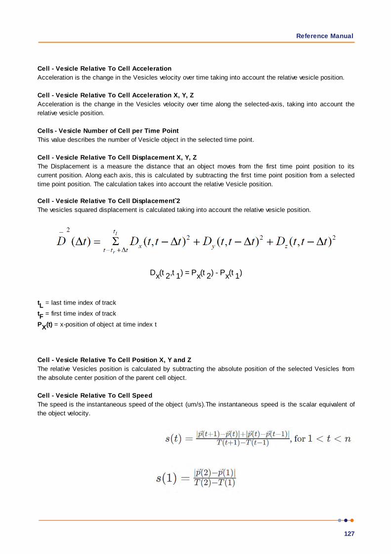
Reference Manual

127

Cell - Vesicle Relative To Cell Acceleration

Acceleration is the change in the Vesicles velocity over time taking into account the relative vesicle position.

Cell - Vesicle Relative To Cell Acceleration X, Y, Z

Acceleration is the change in the Vesicles velocity over time along the selected-axis, taking into account the

relative vesicle position.

Cells - Vesicle Number of Cell per Time Point

This value describes the number of Vesicle object in the selected time point.

Cell - Vesicle Relative To Cell Displacement X, Y, Z



time point position. The calculation takes into account the relative Vesicle position.

Cell - Vesicle Relative To Cell Displacementˆ2

The vesicles squared displacement is calculated taking into account the relative vesicle position.

Dx(t 2,t 1) = Px(t 2) - Px(t 1)




Cell - Vesicle Relative To Cell Position X, Y and Z

The relative Vesicles position is calculated by subtracting the absolute position of the selected Vesicles from

the absolute center position of the parent cell object.

Cell - Vesicle Relative To Cell Speed

The speed is the instantaneous speed of the object (um/s).The instantaneous speed is the scalar equivalent of

the object velocity.

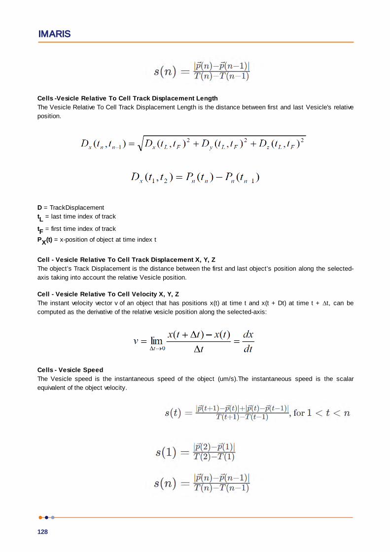
IMARIS

128

Cells -Vesicle Relative To Cell Track Displacement Length

The Vesicle Relative To Cell Track Displacement Length is the distance between first and last Vesicle's relative

position.





Cell - Vesicle Relative To Cell Track Displacement X, Y, Z


axis taking into account the relative Vesicle position.

Cell - Vesicle Relative To Cell Velocity X, Y, Z

The instant velocity vector v of an object that has positions x(t) at time t and x(t + Dt) at time t + t, can be

computed as the derivative of the relative vesicle position along the selected-axis:

Cells - Vesicle Speed

The Vesicle speed is the instantaneous speed of the object (um/s).The instantaneous speed is the scalar


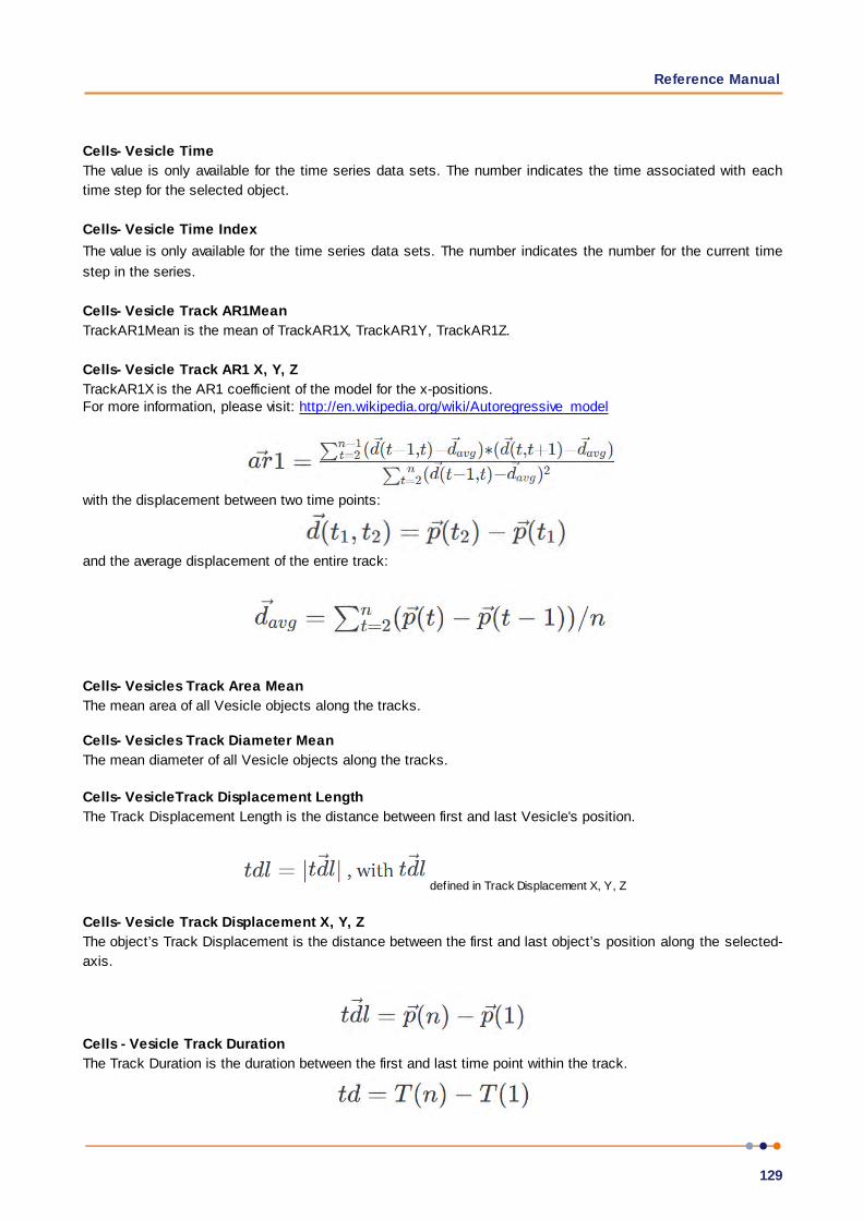
Reference Manual

129

Cells- Vesicle Time



Cells- Vesicle Time Index


step in the series.

Cells- Vesicle Track AR1Mean


Cells- Vesicle Track AR1 X, Y, Z


with the displacement between two time points:

and the average displacement of the entire track:

Cells- Vesicles Track Area Mean

The mean area of all Vesicle objects along the tracks.

Cells- Vesicles Track Diameter Mean

The mean diameter of all Vesicle objects along the tracks.

Cells- VesicleTrack Displacement Length

The Track Displacement Length is the distance between first and last Vesicle's position.


Cells- Vesicle Track Displacement X, Y, Z


axis.

Cells - Vesicle Track Duration



IMARIS

130

Cells- Vesicle Track Intensity Center Mean

This value describes the mean voxel intensity in the center of the Vesicle along the tracks.

Cells- Vesicle Track Intensity Max

This value describes the maximum voxel intensity of the Vesicle along the tracks.

Cells - Vesicle Track Intensity Mean

This value describes the mean voxel intensity of the Vesicle along the tracks.

Cells - Vesicle Track Intensity Median

This value describes the Average of all Intensity Medians of all objects at all time points in the track.

Cells - Vesicle Track Intensity Min

This value describes the minimum voxel intensity of the Vesicle along the tracks.

Cells - Vesicle Track Intensity StdDev

This value describes the Standard Deviation voxel intensity of the Vesicle along the tracks.

Cells - Vesicle Track Intensity Sum

This value describes the sum of voxel intensity of the Vesicle along the tracks.

Cells - Vesicle Track Length


Cells - VesicleTrack Number of Branches


Cells - Vesicle Track Number of Fusions


Cells- Vesicle Tracks Position Mean X, Y, Z

Defines the mean value of X, Y, Z Vesicles track positions.

Cells- Vesicle Tracks Position X, Y, Z Start


Cells- Track Number of Vesicle

The number of the all Vesicles objects along the tracks.

Cells - Vesicle Track Speed Max


Cells - Vesicle Track Speed Mean

The Average value of the object’s speed on the track. If the Track has no Fuses (merges) or fragments (splits),


Track.

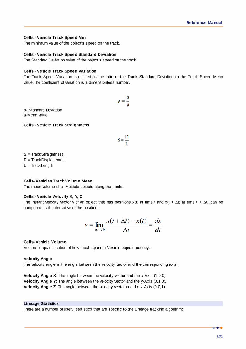
Reference Manual

131

Cells - Vesicle Track Speed Min


Cells - Vesicle Track Speed Standard Deviation


Cells - Vesicle Track Speed Variation




Cells - Vesicle Track Straightness



L = TrackLength

Cells- Vesicles Track Volume Mean

The mean volume of all Vesicle objects along the tracks.

Cells - Vesicle Velocity X, Y, Z

The instant velocity vector v of an object that has positions x(t) at time t and x(t + t) at time t + t, can be

computed as the derivative of the position:

Cells- Vesicle Volume

Volume is quantification of how much space a Vesicle objects occupy.

Velocity Angle

The velocity angle is the angle between the velocity vector and the corresponding axis.

Velocity Angle X: The angle between the velocity vector and the x-Axis (1,0,0).

Velocity Angle Y: The angle between the velocity vector and the y-Axis (0,1,0).

Velocity Angle Z: The angle between the velocity vector and the z-Axis (0,0,1).

Lineage Statistics

There are a number of useful statistics that are specific to the Lineage tracking algorithm:

IMARIS

132

Generations

This shows the generation that the selected object belongs to. This is displayed in the format: 0.00 for the initial

object, e.g. mother cell and 1.00 for the following 1st generation e.g. daughter cells. Tracked objects without

divisions and untracked objects have a generation value of 0.

Track Number of Generations

This statistic shows the number of generations present in the selected track.

Time since first Division

This shows the time elapsed since the first division of the selected object(s).

Time since previous Division

This shows the time between each generation. e.g. the lifespan of an object

Normalized Time since previous Division

Displays the normalized division time. This value is only calculated for objects that have a previous division.

Only defined for objects that have a previous division and a following division and no fuses (merges).

Displacement Since Previous Division

This describes the displacement that has occurred since the previous division. The Displacement 2̂ (plotted

over Time Since Previous Division obtains the “Displacement Squared Plot”) and its individual components X, Y

and Z (which are analogous to the Position statistics). The values are available only for tracked objects after a

track split. If there are multiple objects at the last time point, the most distant one (geometrically) is used for

the calculation.

Time since track start

Displays time since the start of the track. This is only available only for objects that belong to a track. It is

different to time statistics for objects belonging to tracks that do not start from the first time point. It enables the

user to plot the displacement 2̂ over track time start, as in the example at “Displacement Squared Plot” at

http://bradleymonk.com/Brownian_Motion.

Cell Cycle Duration

Time since the previous division for objects that divide again. This is only defined for objects that divide and have

a previous division.

Cell Cycle Displacement

This option introduces multiple values. There is the Cell Cycle Displacement Length, which is equal to the

square root of the Displacement Since Previous Division 2̂ for the last object of a track segment (a track

segment is any piece of track that has no bifurcations, a track without bifurcations is constituted by a single

segment), and there are the individual components X, Y and Z. As with Track Cycle Duration, the values are

only added to the last object of a segment.

5.9.9.2 FilamentStatistic Values - Filament

A simplified representation of the dendritic tree is shown below with (•) representing a dendritic vertex, and (x) aspine vertex. Dendrite and Spine edges are represented with (—) or (....) respectively. Dendrite segments arenoted with D and spine segments with S.

http://bradleymonk.com/Brownian_Motion

Reference Manual

133

Figure 1

Filaments - Dendrite Area

This may be defined as the sum of the areas of all the dendrites segment edges.

The area of an edge is defined as a surface area of a frustum (truncated cone).

Figure 2

A = A(i)2, i = 0,...n - 1,n

n = number of edges of a segment

Filaments - Dendrite Branch Depth

Branching Depth is defined as the number of branch points, or bifurcations, in the shortest path from the

beginning point to a given point in the dendritic graph.

IMARIS

134

Filaments - Dendrite Branch Level

The Dendrite Branch Level is a numerical structure that starts unfolding from the filament beginning toward the

terminal points, assigning Branch Level to dendrite segments at each branching point.

The Branch Level number is assessed according to the diameter calculations of the individual dendrite

segments. The initial Branch Level at the beginning point is 1. At each branching point, the dendrite segment

with smaller mean diameter sequentially increases Branch Level, while the dendrite segment with a greater

diameter maintains the same Branch Level.

In the case of two dendrite segments with the same diameter, the segment with a smaller Branching Angle

(refer to Figure 4) keeps the Branch Level, while the dendrite segment with a greater Branching Angle

sequentially raises its Branch Level.

In the Figure 3 diameter d1 is greater than d

2 (d

1 >d

2) and d

3 and d

4 are equal (d

3 = d

4). The Dendrite Branching

Angle 1 is smaller than

2 (

1 <

2).

Figure 3

• represents a dendritic vertex

Filaments - Dendrite Branching Angle

Defined as the angle between the extending lines from the branch point and its peripheral neighbor vertex

(Figure 4 angles marked with dashed blue arcs, 1 for dendrite segment D1 and

2 for dendrite segment D2).

Defined only if the beginning point is determined.

Reference Manual

135

Figure 4

Please note • represents a dendritic vertex

Filaments - Dendrite Branching Angle B

The angle between the extending lines connecting the branch point with the neighboring branch points and the

terminal points, respectively (Figure 5 angles marked with dashed green arcs, ). Defined only if the beginning

point is determined.

Figure 5


Filaments -Dendrite Length

Defined as the sum of all edges between two branch points or between a branch point and a terminal point,

respectively. (Figure 2 Dendrite Length e0+e1+e2).

Filaments -Dendrite Mean Diameter

The mean value of all dendrites diameters measured from the center to the dendrite surfaces using the lower

threshold (automatic creation) value.

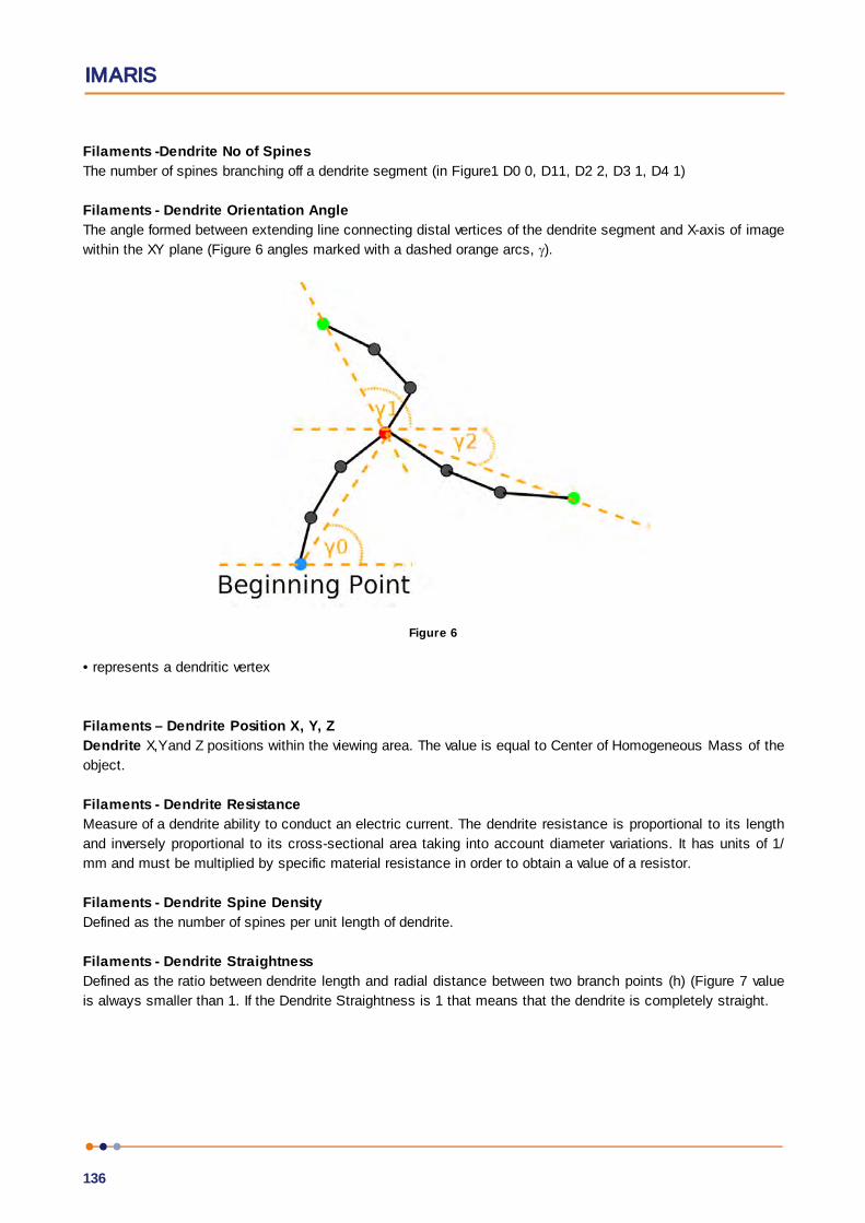
IMARIS

136

Filaments -Dendrite No of Spines

The number of spines branching off a dendrite segment (in Figure1 D0 0, D11, D2 2, D3 1, D4 1)

Filaments - Dendrite Orientation Angle

The angle formed between extending line connecting distal vertices of the dendrite segment and X-axis of image

within the XY plane (Figure 6 angles marked with a dashed orange arcs, ).

Figure 6


Filaments – Dendrite Position X, Y, Z

Dendrite X,Yand Z positions within the viewing area. The value is equal to Center of Homogeneous Mass of the

object.

Filaments - Dendrite Resistance

Measure of a dendrite ability to conduct an electric current. The dendrite resistance is proportional to its length

and inversely proportional to its cross-sectional area taking into account diameter variations. It has units of 1/

mm and must be multiplied by specific material resistance in order to obtain a value of a resistor.

Filaments - Dendrite Spine Density

Defined as the number of spines per unit length of dendrite.

Filaments - Dendrite Straightness

Defined as the ratio between dendrite length and radial distance between two branch points (h) (Figure 7 value

is always smaller than 1. If the Dendrite Straightness is 1 that means that the dendrite is completely straight.

Reference Manual

137

Figure 7


Filaments - Dendrite Time



Filaments - Dendrite Time Index


step in the series.

Filaments - Dendrite Volume

Defined as the sum of all (frustum) volumes composing a dendrite (Figure 2).

V = V(i) i- 0,...n - 1,n

n =number of edges of a segment

Filaments - Filament Acceleration

Acceleration is the change in the filament graph velocity over time.

Object position at time-point i:

Acceleration vector x, y, z at time-point i

Acceleration at time-point i:

a(i) = |A(i)|


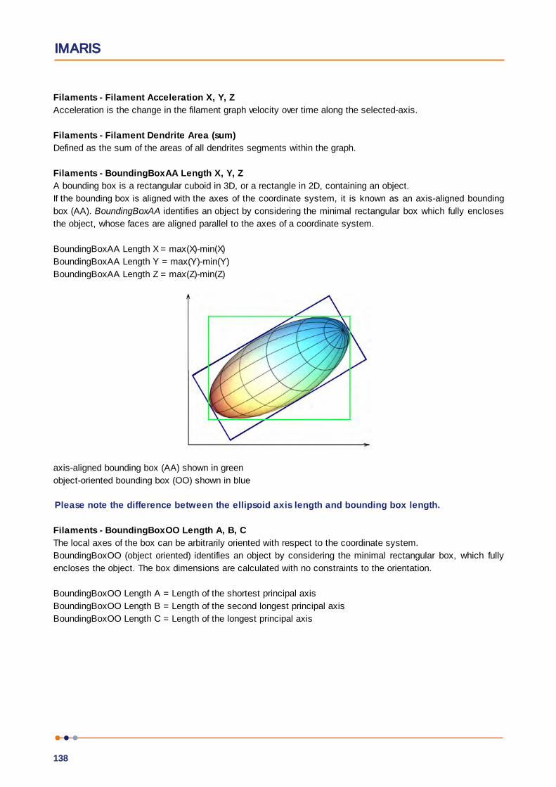
IMARIS

138

Filaments - Filament Acceleration X, Y, Z

Acceleration is the change in the filament graph velocity over time along the selected-axis.

Filaments - Filament Dendrite Area (sum)

Defined as the sum of the areas of all dendrites segments within the graph.

Filaments - BoundingBoxAA Length X, Y, Z











Filaments - BoundingBoxOO Length A, B, C







Reference Manual

139




Filaments - Filament Dendrite Area (sum)

The sum of all dendrites areas of within the entire filament graph.

Filaments - Filament Dendrite Length (sum)

The sum of all dendrites length of within the entire filament graph.

Filaments - Filament Dendrite Volume (sum)

The sum of the volumes of all dendrites within the entire filament graph.

Filaments - Filament Displacement X, Y, Z




Filaments - Filament Displacement 2

The square of the distance of the object from the starting point of the track (also known as mean square

displacement: MSD) when plotted against the relative time since the beginning of the track

D 2̂(t – t_F) = Dx(t, t_F) 2̂ + Dy(t, t_F) 2̂ + Dz(t, t_F) 2̂

Dx(t 2,t 1) = Px(t 2) - Px(t 1)


Px(t) = x-position of object at time index t

Filaments - Filament Full Branch Depth

Branch Depth is defined as the number of branch points, or bifurcations, in the shortest path from the beginning

point to a given point in the filament graph. Full Branch Depth is the highest value of Branching Depth for the

graph (in Figure 1 value is 2). If no beginning point is defined, the value is set to "-1" (Figure1).

Filaments - Filament Full Branch Level

Full Branch Level is the highest value of Branching Level for the entire filament graph (in Figure 3 value is 4).

Filaments - Filament Length (Sum)

Defined as the sum of the lengths of all edges (both dendrites and spines) within the entire graph.

IMARIS

140

Filaments - Filament No. Dendrite Branch Points

The number of dendrites branching points in the entire filament graph (in Figure1 value is 3).

Filaments - Filament No. Dendrites Branches

The statistics are defined for a filament and a distance value. This is calculated by following the filament from

the beginning point along all dendrites for the defined distance, and then counting how many different branches

have been reached. Imaris calculates this as follows:

Distances 0 to n * DistanceIncrement

where DistanceIncrement has a default value of 1 m and n is dependent on the maximum dendrite terminal

point distance to the beginning point of the filament. Note that the DistanceIncrement is equal to the "Sholl

Spheres Resolution" and can be adjusted in the Statistics Preferences. The different distance values are visible

as Factors "Distance" of the statistics value.

Figure 8 Filament w ith 7 dendrites, beginning point at the bottom left and indicators marking the dendrite branches

for different distances

Value Distance

0 0

1 1

2 2

3 3

2 4

0 5

Filaments - Filament No. Dendrite Segments

The number of dendrite segments in the entire filament graph (Figure 1 value is 8).

Filaments - Filament No. Dendrite Terminal Points

The number of dendrite terminal points (excluding the beginning point) in the entire filament graph (Figure 1

value is 6).

Filaments - Filament No. Edges

The number of connections between vertices in the entire filament graph (Figure 1 value is 34).

Reference Manual

141

Filaments - Filament No. Sholl Intersections

Sholl analysis creates a series of concentric circles (spheres in 3D) around the beginning point of the filament.

Filament No. Sholl Intersections is defined as the number of dendrite intersections (branches) on concentric

spheres, defining dendrite spatial distribution as a function of distance from the beginning point. All spheres

have a center at the beginning point (Figure 9). The 1.0 um step resolution for the spheres can be changed

under Preferences -> Advanced -> SurfaceAppFilament

Figure 9

Filaments - Filament No. Spine Branching Points

The number of spine branch points in the entire filament graph (in Figure 1 value is 1). A spine branch point will

only exist in a single spine that has more than one terminal point.

IMARIS

142

Filaments - Filament No. Spine Segments

The spine segment count in entire filament graph (in Figure 1 value is 7).

Filaments - Filament No. Spine Terminal Points

The number of spine terminal points in the entire filament graph (in Figure 1 value is 6).

Filaments - Filament No. Unconnected Parts

The number of unconnected filament graph within the image.

Filaments - Filament No. Vertices

The number of vertices in the filament graph (Figure 1 value is 36).

Filaments – Filament Number of Filament pre Time Points

Totals number of filament graph within the image at the specific time point.

Filaments – Filament Number of Tracks

Totals number of tracks for the selected filament graph.

Filaments – Filament Position X, Y, Z

Filament graph X, Y, Z position within the viewing area. The value is equal to Center of Homogeneous Mass of

the object.

Filaments – Filament Speed

The filament speed is the instantaneous speed of the object (um/s).The instantaneous speed is the scalar


Filaments - Filament Spine Area (sum)

Defined as the sum of the areas of all spines segments within the filament graph.

Filaments -Filament Spine Length (sum)

The sum of all spines length of within the entire filament graph.

Filaments -Filament Spine Volume (sum)

The sum of the volumes of all spines within the entire filament graph.

Filaments -Filament Time



Reference Manual

143

Filaments -Filament Time Index


step in the series.

Filaments -Filament Total Number of Filaments

The value indicates the total number of filament graph within the data set.

Filaments -Filament Track AR1Mean


Note for all track statistics splits or gaps are not taken into account- it is taken that the selected tack is

continuous.

Filaments -Filament Track AR1 X, Y, Z

TrackAR1X is the AR1 coefficient of the model for the x-positions.

AR1X = TrackAR1X



Dx(t2,t1) = Px(t2) - Px(t1)





For more information, please visit: http://en.wikipedia.org/wiki/Autoregressive_model

Filaments - Filament Track Displacement Length

The Track Displacement Length is the distance between first and last filament graph position.


IMARIS

144

Dx(t

F,t

L) = Px(t

L) - Px(t

F)





Filaments - Filament Track Displacement X, Y, Z


axis.

Filaments - Filament Displacement Delta XYZ


Filaments - Filament Displacement Delta Length (a scalar value)


Filaments - Filament Track Duration


Duration = T(tL) - T (t

F)

Duration = TrackDuration

T(t) = time in seconds at time point t



Filaments - Filament Track Length

The Track Length is the total length of displacements along the track.

L = TrackLength



Dx(tf,t l) = Px(t l) - Px(t f)

Reference Manual

145

Filaments -Filament Track No. Dendrites Branches

The number of parallel outstretched dendritic branches counted from the beginning point toward the terminal

points at constant length increments along the selected track.

Filaments - Filament Track Number of Filaments

The total number of filament graphs along the track.

Filaments - Filament Track Number of Fusions

A fusion occurs when a filament object is connected to several filament objects of a past time point. The value

indicates the number of the related objects.

Filaments - Filament Track Position X, Y, Z Mean

Defines the mean value of X, Y, Z Track positions.

Filaments - Filament Tracks Position X, Y, Z Start


Filaments - Filament Track Speed Max


Filaments -Filament Track Speed Mean

The Average value of the object’s speed on the track. If the Track has no fuses (merges) or fragments (splits),


Track.

Filaments -Filament Track Speed Min


Filaments - Filament Track Speed Standard Deviation


Filaments - Filament Track Speed Variation




Filaments - Filament Track Straightness



L = TrackLength

IMARIS

146

Filaments - Filament Velocity X, Y, Z

Velocity is the rate of change of object displacement with time. Speed and velocity are related in the same way

as distance and displacement. Speed is a scalar and velocity is a vector.

The formula for calculating the velocity at time point is calculated as follows:

For objects at time point at the beginning of a track the velocity is computed from the position and

time t of the object at time point and :

For objects at time point in the middle of a track the velocity is computed from the position and time

t of the object at time point and :

For objects at time point at the end of a track the velocity is computed from the position and time t

of the object at time point and :

Filaments - Filament Volume (sum)

Volume is the quantity of three-dimensional space occupied by an object. The sum of all segment's volumes

within the entire filament graph.

Filaments - Pt Acceleration

Acceleration is the change in the object velocity over time.




a(i) = |A(i)|

Reference Manual

147


Filaments - Pt Acceleration X, Y, Z

Acceleration is the change in the filament points velocity over time along the selected-axis.

Filaments - Pt Branching Angle

The angle between the lines connecting the branch point with either of its two neighboring peripheral vertices (in

Figure 10 a angles are marked with ). This value is defined only for filament graphs with a valid beginning point.

If the beginning point has not been defined then Pt. Branching Angle is the smallest of the angles between the

branching segments (in Figure 10 b angles marked with 2). The value is not calculated for branch points with

more than three segments.

Figure 10

Filaments - Pt Spine Total Length

This is defined as the sum of the Length of all Spines connected to the Spine Attachment Point.

Filaments - Pt Spine Total Area

This is defined as the sum of the Area of all Spines connected to the Spine Attachment Point.

Filaments - Pt Spine Total Volume

This is defined as the sum of the Volume of all Spines connected to the Spine Attachment Point.

Filaments - Pt Diameter

Defined as the value of the vertices’s diameter (Figure 2).

Filaments - Pt Displacement X, Y, Z




Filaments - Pt Displacement ^2

IMARIS

148

Dx(t f,t l) = Px(t l) - Px(t f)




Filaments - Pt Displacement Delta XYZ


Filaments - Pt Displacement Delta Length (a scalar value)


Filaments - Pt Distance

Distance of the specific vertex from the beginning point along the dendritic graph structure (Figure 8).

Filaments - Pt Number of Points per Time Point

Number of all beginning, branching, attachment and terminal points in the selected time point.

Filaments - Pt Position X, Y, Z

The X, Y, Z coordinates of all tracked beginning, branching, attachment and terminal points.

These values are only available if the tracking option is selected.

Filaments - Pt Speed

The filaments - Pt speed is the instantaneous speed of the object (um/s).The instantaneous speed is the scalar


Filaments -Pt Time



Filaments -Pt Time Index


step in the series.

Filaments -Pt Total Number of Points

Number of all beginning, branching, attachment and terminal points.

Reference Manual

149

Filaments - Pt Track AR1Mean


Filaments - Pt Track AR1 X, Y, Z

TrackAR1X is the AR1 coefficient of the model for the x positions.

AR1X = TrackAR1X



Dx(t2,t1) = Px(t2) - Px(t1)





Filaments - Pt Track Displacement Length

The Track Displacement Length is the distance between first and last point position.

Dx(t

F,t

L) = Px(t

L) - Px(t

F)





Filaments - Pt Track Displacement X, Y, Z


IMARIS

150


axis.

Filaments - Pt Track Duration


Duration = T(tL) - T(t

F)

Duration = TrackDuration

T(t) = time in seconds at time point t



Filaments - Pt Track Length

The Track Length is the total length of displacements along the track.

L = TrackLength



Dx(t

F,t

L) = Px(t

L) - Px(t

F)

Note for all track statistics splits or gaps are not taken into account- it is taken that the selected tack

is continuous.

Filaments - Pt Track No. Dendrites Branches

The number of parallel outstretched dendritic branches counted from the beginning point toward the terminal

points at constant length increments along the selected track.

Filaments - Pt Track Number of Fusions

A fusion occurs when a filament graph beginning, branching, attachment and terminal points are connected to

several graph key points of a past time point. The value indicates the number of the related objects along the

selected track.

Filaments - Pt Track Number of Points

The total number of points (beginning, branching, attachment and terminal) along the track.

Filaments - Pt Track Position X, Y, Z Mean

Defines the mean value of X, Y, Z Track positions.

Filaments - Pt Tracks Position X, Y, Z Start

Defines the value of the X, Y, Z track start positions

Filaments - Pt Track Speed Max

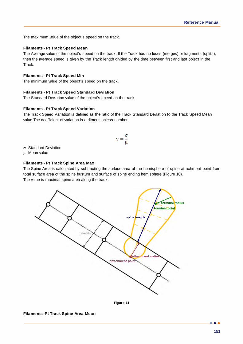
Reference Manual

151


Filaments - Pt Track Speed Mean

The Average value of the object’s speed on the track. If the Track has no fuses (merges) or fragments (splits),


Track.

Filaments - Pt Track Speed Min


Filaments - Pt Track Speed Standard Deviation


Filaments - Pt Track Speed Variation



- Standard Deviation- Mean value

Filaments - Pt Track Spine Area Max

The Spine Area is calculated by subtracting the surface area of the hemisphere of spine attachment point from

total surface area of the spine frustum and surface of spine ending hemisphere (Figure 10).

The value is maximal spine area along the track.

Figure 11

Filaments -Pt Track Spine Area Mean

IMARIS

152



The value is mean spine area along the track.

Filaments - Pt Track Spine Area Min



The value is minimal spine area along the track.

Filaments - Pt Track Spine Length Max

The value is the maximal spine length (see definition of the Spine Length statistics value) of all spines that are

part of the track.

Filaments - Pt Track Spine Length Min

The value is the minimal spine length (see definition of the Spine Length statistics value) of all spines that are

part of the track.

Filaments - Pt Track Spine Length Mean

The value is the mean spine length (see definition of the Spine Length statistics value) of all spines that are part

of the track.

Filaments - Pt Track Spine Volume Max

The Spine volume is calculated by subtracting the hemisphere volume of the spine attachment point from the

total volume of the spine frustum and volume of the spine ending hemisphere (Figure 11).

The value is maximal spine volume along the track.

Filaments - Pt Track Spine Volume Min



The value is minimal spine volume along the track.

Filaments - Pt Track Spine Volume Mean



The value is mean spine volume along the track.

Filaments - Pt Track Spine Straightness

Defined as the ratio between spine length and radial distance between two branch points (h) (defined in the

same way as Dendrite Straightness, refer to Figure 7).

Filaments - Pt Velocity X, Y, Z


as distance and displacement. Speed is a scalar and velocity is a vector. The instant velocity vector v of an

object that has positions x(t) at time t and x(t + dt) at time t + t, can be computed as the derivative of the

relative object position along the selected-axis:

Filaments - Spine Area

Reference Manual

153



Filaments - Spine Attachment Pt Acceleration





a(i) = |A(i)|


Filaments - Spine Attachment Pt Acceleration X, Y, Z


Filaments - Spine Attachment Pt Branching Angle

The angle between the lines connecting the branch point with either of its two neighboring peripheral vertices (in

Figure 10 a angles are marked with ). This value is defined only for filament graphs with a valid beginning point.

If the beginning point has not been defined then Pt. Branching Angle is the smallest of the angles between the

branching segments (in Figure 10 b angles marked with 2). The value is not calculated for branch points with

more than three segments.

Filaments - Spine Attachments Pt Diameter

Diameter of a vertex at the spine attachment point to the dendrite.

Filaments - Spine Attachments Pt Displacement X, Y, Z




Filaments - Spine Attachments Pt Displacement ^2

IMARIS

154





Filaments - Spine Attachments Pt Distance


Filaments - Spine Attachments Pt Position X, Y, Z



Filaments - Spine Attachments Pt Speed

The object speed is instantaneous speed of the graph beginning, branching, attachment and terminal points

(um/s).The instantaneous speed is the scalar equivalent of the object velocity.

Filaments - Spine Attachments Pt Time



Filaments - Spine Attachments Pt Time Index


step in the series.

Filaments - Spine Attachments Velocity X, Y, Z



object that has positions x(t) at time t and x(t + Dt) at time t + t, can be computed as the derivative of the


Filaments - Spine Branch Depth

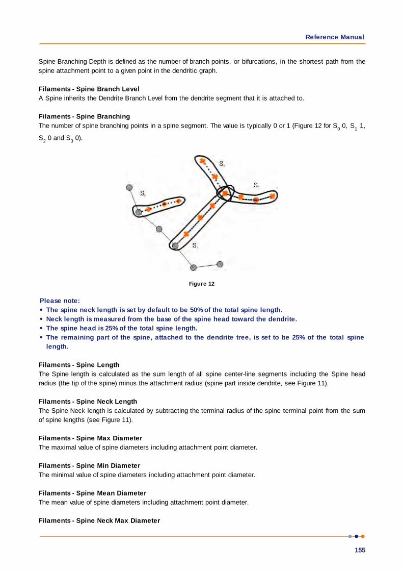
Reference Manual

155

Spine Branching Depth is defined as the number of branch points, or bifurcations, in the shortest path from the

spine attachment point to a given point in the dendritic graph.

Filaments - Spine Branch Level

A Spine inherits the Dendrite Branch Level from the dendrite segment that it is attached to.

Filaments - Spine Branching

The number of spine branching points in a spine segment. The value is typically 0 or 1 (Figure 12 for S0 0, S

1 1,

S2 0 and S

3 0).

Figure 12

Please note:

The spine neck length is set by default to be 50% of the total spine length.

Neck length is measured from the base of the spine head toward the dendrite.

The spine head is 25% of the total spine length.

The remaining part of the spine, attached to the dendrite tree, is set to be 25% of the total spine

length.

Filaments - Spine Length

The Spine length is calculated as the sum length of all spine center-line segments including the Spine head

radius (the tip of the spine) minus the attachment radius (spine part inside dendrite, see Figure 11).

Filaments - Spine Neck Length

The Spine Neck length is calculated by subtracting the terminal radius of the spine terminal point from the sum

of spine lengths (see Figure 11).

Filaments - Spine Max Diameter

The maximal value of spine diameters including attachment point diameter.

Filaments - Spine Min Diameter

The minimal value of spine diameters including attachment point diameter.

Filaments - Spine Mean Diameter

The mean value of spine diameters including attachment point diameter.

Filaments - Spine Neck Max Diameter

IMARIS

156

Filaments - Spine Neck Mean Diameter

Filaments - Spine Neck Min Diameter

Maximum, Mean and Minimum value of the spine neck diameter (excluding the spine attachment and terminal

pints diameters).

Filaments - Spine Neck Volume

The Spine Neck volume is calculated by subtracting the volume of the spine-ending hemispheres (attachment

and terminal point) from the spine volume.

Filaments - Spine Orientation Angle

The angle formed between the extending line connecting distal spine vertices in the spine segment and X-axis

of the image within the XY plane (defined in the same way as Dendrite Orientation Angle, refer to Figure 6).

Filaments - Spine Part Length Ground

The spine ground length is set by default to be 25% of the total spine vertices (points).

Filaments - Spine Part Length Head

The spine head length is set by default to be 25% of the total spine length.

Filaments - Spine Part Length Neck

The spine neck length is set by default to be 50% of the total spine length.

Filaments - Spine Part Max Diameter Ground

The maximal value of the spine ground diameter.

Filaments - Spine Part Max Diameter Head

The maximal value of the spine head diameter.

Filaments - Spine Part Max Diameter Neck

The maximal value of the spine neck diameter.

Filaments - Spine Part Mean Diameter Ground

The average value of the spine ground diameter.

Filaments - Spine Part Mean Diameter Head

The average value of the spine head diameter.

Filaments - Spine Part Mean Diameter Neck

The average value of the spine neck diameter.

Filaments - Spine Part Min Diameter Ground

The minimal value of the spine ground diameter.

Filaments - Spine Part Min Diameter Head

The minimal value of the spine head diameter.

Filaments - Spine Part Min Diameter Neck

The minimal value of the spine neck diameter.

Filaments - Spine Part Volume Ground

Measure the volume of the spine ground.

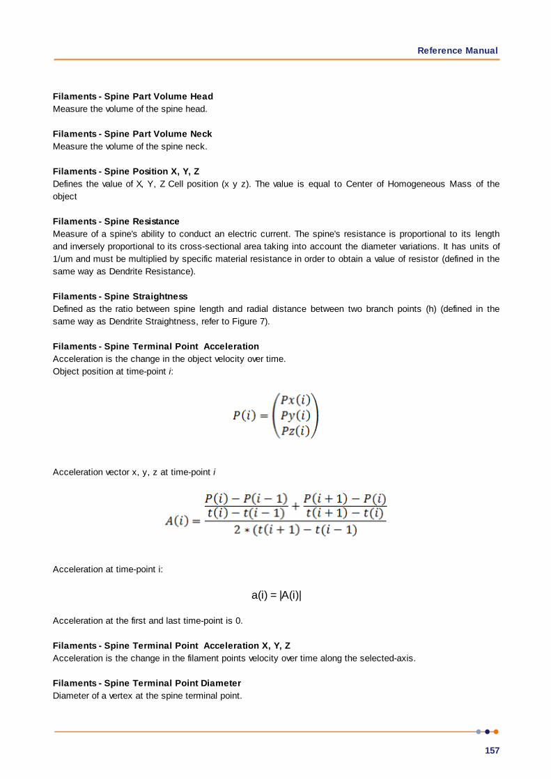
Reference Manual

157

Filaments - Spine Part Volume Head

Measure the volume of the spine head.

Filaments - Spine Part Volume Neck

Measure the volume of the spine neck.

Filaments - Spine Position X, Y, Z

Defines the value of X, Y, Z Cell position (x y z). The value is equal to Center of Homogeneous Mass of the

object

Filaments - Spine Resistance

Measure of a spine's ability to conduct an electric current. The spine's resistance is proportional to its length

and inversely proportional to its cross-sectional area taking into account the diameter variations. It has units of

1/um and must be multiplied by specific material resistance in order to obtain a value of resistor (defined in the

same way as Dendrite Resistance).

Filaments - Spine Straightness

Defined as the ratio between spine length and radial distance between two branch points (h) (defined in the

same way as Dendrite Straightness, refer to Figure 7).

Filaments - Spine Terminal Point Acceleration





a(i) = |A(i)|


Filaments - Spine Terminal Point Acceleration X, Y, Z


Filaments - Spine Terminal Point Diameter

Diameter of a vertex at the spine terminal point.

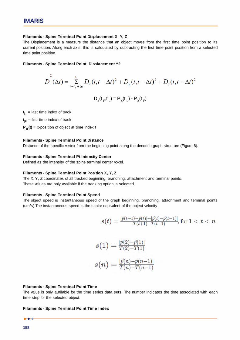
IMARIS

158

Filaments - Spine Terminal Point Displacement X, Y, Z




Filaments - Spine Terminal Point Displacement ^2

Dx(t

F,t

L) = Px(t

L) - Px(t

F)




Filaments - Spine Terminal Point Distance


Filaments - Spine Terminal Pt Intensity Center

Defined as the intensity of the spine terminal center voxel.

Filaments - Spine Terminal Point Position X, Y, Z



Filaments - Spine Terminal Point Speed

The object speed is instantaneous speed of the graph beginning, branching, attachment and terminal points

(um/s).The instantaneous speed is the scalar equivalent of the object velocity.

Filaments - Spine Terminal Point Time



Filaments - Spine Terminal Point Time Index

Reference Manual

159


step in the series.

Filaments - Spine Terminal Point Velocity X, Y, Z



object that has positions x(t) at time t and x(t + Dt) at time t + t, can be computed as the derivative of the


Filaments -Spine Terminal Pt. Volume

Spine Terminal Pt. Volume is calculated as a volume of the sphere with the diameter of a spine terminal point

vertex (Figure 11).

Filaments - Spine Time



Filaments - Spine Time Index


step in the series.

Filaments - Spine Volume



Velocity Angle





5.9.9.3 Measurement PointsMeasurement Point statistics are automatically computed for each Measurement Point.

Show Statistic Values - Measurement Points

Measurement Points - Angle

This is the angle between two adjacent measurement points that share a common point. This statistic is only

calculated in Polygon (ABCD…) Line Mode.

Measurement Points - Distance

This is the distance between the measurement points.

Measurement Points - Distance Sum

The Distance Sum is the sum of all measured distances.

IMARIS

160

Measurement Points - Number of Points

This is defined as the number of measurement points.

Measurement Points - Point Intensity Center

The Point Intensity Center is the value of the point intensity center (average) in the different channels.

Measurement Points - Point Position X

Point position in x-axis.

Measurement Points - Point Position Y

Point position in y-axis.

Measurement Points - Point Position Z

Point position in z-axis.

5.9.9.4 SpotsSpots statistics can be located in the statistics tab. Spots store a diameter and a specific time point. The

intensity of the spot is defined by their statistics, intensity therefore changes when the image changes, which

means that it is not an inherent part of the Spot itself (and not given a different treatment than the other

statistics). Position X Y Z, diameter X Y Z and the time point are the values needed for the full description of a

Spot. These values can be edited in the Edit tab options.

Show Statistic Values - Spots

Spots- Acceleration

Acceleration is the change in the Spot(s) velocity over time.




The acceleration at the first and last time-point is 0.

Spots- Acceleration X, Y, Z

The acceleration is the change in the velocity of a spot over time along the selected-axis.

Spots - Area

The sum of the area of the sphere / ellipsoid surface (surface of the spot).

Spots - Diameter X, Y, Z

The diameter specifies the size of spherical object (i.e. the spot) along the selected-axis.

Reference Manual

161

Spots - Displacement X, Y, ZThe Displacement is a measure of the distance that a spot moves from the first time point position, to its

current position. This is calculated for each axis by subtracting the first time point position from a selected time

point position:

Spots - Displacement ^2

The square of the distance of the spot from the starting point of the track (also known as mean square

displacement: MSD) when plotted against the relative time since the beginning of the track:


Spots - Intensity Center

The Intensity Center is the intensity of the voxel at the center of the Spot.

Spots - Intensity Max

Spots - Intensity Mean

Spots - Intensity Median

The Spots - intensity median is estimated from the intensity histogram.

Spots - Intensity Min

Spots - Intensity StdDev

Spots - Intensity Sum

The spots intensity statistics provide a description for the voxels enclosed within a Spot (Max, Mean, Median,


Spots - Number of Spots per Time Point

This is the number of spots at each time point.

Spots - Number of Tracks

Number of tracks.

Spots - Number of Voxels

Number of voxels within a Spot. A voxel is considered in a spot object if the centre of the voxel is located within

the spot. When spots have a small diameter compared to the voxel size, this statistic value can be 0

Tip: When spots with voxel count 0 are reported it can help to resample the image in the z direction

so that the voxel z size is smaller than the spot diameter

Spots - Position X, Y, Z

The position specifies the spot position (X, Y, Z). The position of the center of the spot:

Spots - Speed

The spots speed is the instantaneous speed of the spot s(t) (µm/s).The instantaneous speed is the scalar


IMARIS

162

Spots - Time



Spots - Time Index


step in the series

Spots - Total Number of Spots

The total number of spot objects.

Spots - Track AR1Mean

TrackAR1Mean is the mean of TrackAR1X, TrackAR1Y and TrackAR1Z.

Note for all track statistics, any splits or gaps are not taken into account- it is taken that the selected

track is continuous in nature.

Spots - Track AR1 X, Y, Z


with the displacement between two time points:

and the average displacement of the entire track:

Spots - Track Area Mean

The mean of the triangle Spots surfaces along the track.

Spots - Track Diameter Mean

The mean diameter of all spots along the track.

Track Displacement X, Y, Z


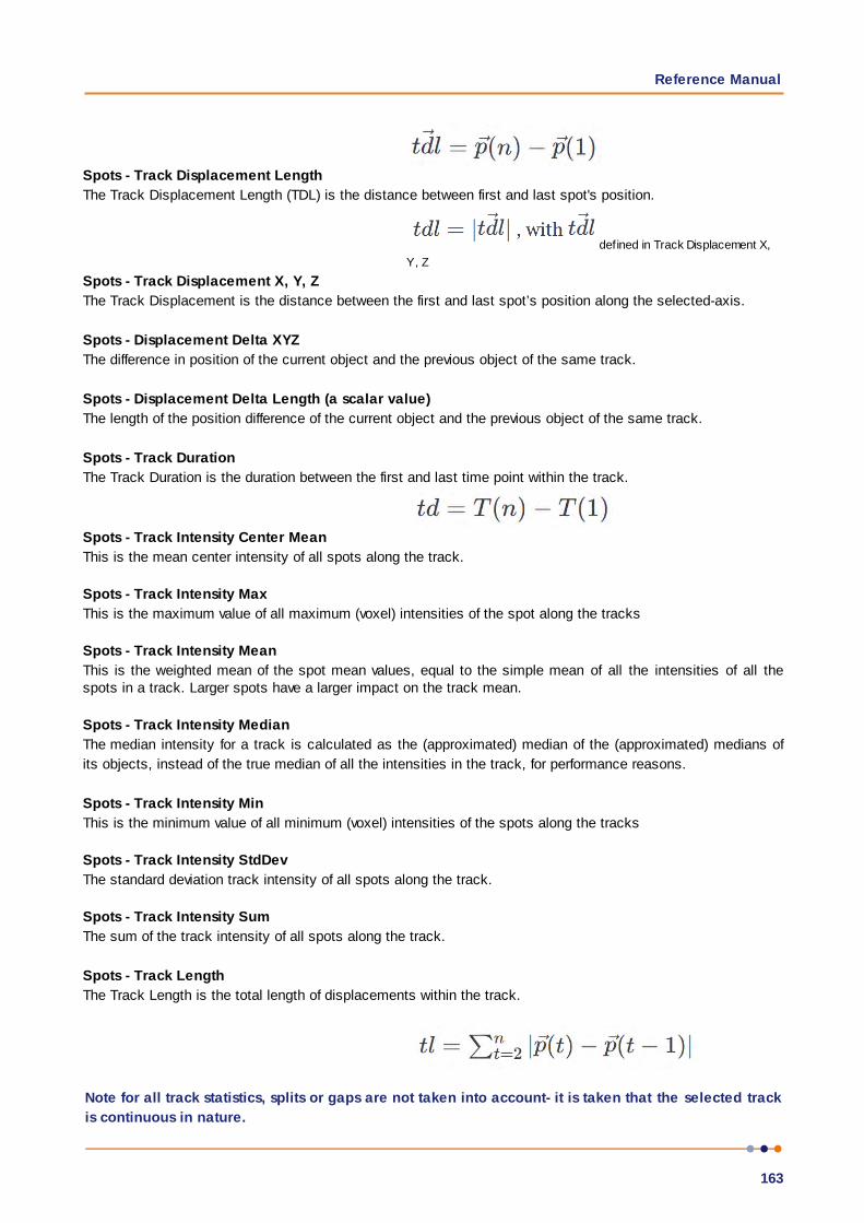
Reference Manual

163

Spots - Track Displacement Length

The Track Displacement Length (TDL) is the distance between first and last spot's position.

defined in Track Displacement X,

Y, Z

Spots - Track Displacement X, Y, Z

The Track Displacement is the distance between the first and last spot’s position along the selected-axis.

Spots - Displacement Delta XYZ


Spots - Displacement Delta Length (a scalar value)


Spots - Track Duration


Spots - Track Intensity Center Mean

This is the mean center intensity of all spots along the track.

Spots - Track Intensity Max

This is the maximum value of all maximum (voxel) intensities of the spot along the tracks

Spots - Track Intensity Mean

This is the weighted mean of the spot mean values, equal to the simple mean of all the intensities of all thespots in a track. Larger spots have a larger impact on the track mean.

Spots - Track Intensity Median

The median intensity for a track is calculated as the (approximated) median of the (approximated) medians of


Spots - Track Intensity Min

This is the minimum value of all minimum (voxel) intensities of the spots along the tracks

Spots - Track Intensity StdDev

The standard deviation track intensity of all spots along the track.

Spots - Track Intensity Sum

The sum of the track intensity of all spots along the track.

Spots - Track Length




IMARIS

164

Spots - Track Number of Branches


Spots - Track Number of Fusions


Spots - Track Number of Spots

The number of track Spots.

Spots - Tracks Position Mean X, Y, Z

Define the mean value of X, Y, Z track coordinates positions.

Spots - Tracks Position X, Y, Z Start

Define the value of the X, Y, Z track start positions.

Spots - Track Speed Max


Spots - Track Speed Mean

The Average value of the spot’s speed on the track. If the Track has no fuses (merges) or fragments (splits),


Track.

Spots - Track Speed Min

The minimum value of the spot’s speed on the track.

Spots - Track Speed Standard Deviation

The Standard Deviation value of the spot’s speed on the track.

Spots -Track Speed Variation




Spots - Track Straightness



L = TrackLength

Spots - Track Volume Mean

The mean volume of all Spots along the tracks.

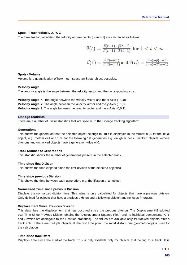
Reference Manual

165

Spots - Track Velocity X, Y, Z


Spots - Volume

Volume is a quantification of how much space an Spots object occupies.

Velocity Angle





Lineage Statistics


Generations


















the calculation.



IMARIS

166




Cell Cycle Duration









5.9.9.5 SurfacesSurfaces statistics are automatically computed for each Surface. These values can be viewed in the statistics

tab.

Show Statistic Values - Surfaces

Surfaces - Acceleration

Acceleration is the change in the Surface velocity over time.

Acceleration X, Y and Z are the components of the acceleration vector (at time-point t):


as defined inAcceleration X, Y, Z

The acceleration at the first and last time-point is 0.

Surfaces - Acceleration X, Y, Z

Acceleration is the change in the Surfaces velocity over time along the selected-axis.

Surfaces - AreaThe sum of the triangle surfaces.

Surfaces - BoundingBoxAA Length X, Y, ZA bounding box is a rectangular cuboid in 3D, or a rectangle in 2D, containing an object.





Reference Manual

167







Surfaces - BoundingBoxOO Length A, B, CThe local axes of the box can be arbitrarily oriented with respect to the coordinate system.








Please note the difference between the ellipsoid axis length and bounding box length

IMARIS

168

Surfaces - Center of Homogeneous Mass X, Y, ZThe voxel intensity values are taken to be the ‘mass’ of each voxel.

The algorithm assumes that every voxel has the same intensity ( i.e. voxel intensities are homogenous).

Assuming a homogeneous intensity, the center of the homogeneous mass is the X, Y, Z coordinate of the

object's centroid (geometric center) .






R : center of homogeneous mass (X, Y, Z)


i z

i)


Surfaces - Center of Image Mass X, Y, ZThe voxel intensity values are taken to be the ‘mass’ of each voxel.








channel separately.


R : center of image mass (x y z)



i z

i)


Surfaces - Displacement X, Y, ZThe Displacement is a measure the distance that an object moves from the first time point position to its


time point position:

Reference Manual

169

Surfaces - Displacement ^2The square of the distance of the object from the starting point of the track (also known as mean square

displacement: MSD) when plotted against the relative time since the beginning of the track:


Surfaces - Distance to Image Border X, YSurfaces - Distance to Image Border X, Y, ZThe value specifies the inward distances from the image border to be removed.

Ellipsoid Axis

In mathematics, an Ellipsoid is a type of quadric that is a higher dimensional analogue of an Ellipse.

The equation of a standard Ellipsoid in an x-y-z Cartesian coordinate system is:

where a, b and c (the lengths of the three semi-axes) are fixed positive real numbers determining the shape of

the Ellipsoid.

Fitting ellipsoid into the surface

To calculate the dimension of a three principal axes of the best-fitted ellipsoid into the surface, the moments of

inertia along the axes of ellipsoid is computed and optimized to match the moment of inertia of the surface. The

ellipsoid has homogeneous mass distribution within the surface object. For more information:

http://en.wikipedia.org/wiki/Moment_of_inertia#Principal_moments_of_inertia

Please note: Only if the shape of the surface matches to an ellipsoid, the lengths of the three

ellipsoid axes are exactly equal to the surface axis.

Surfaces - Ellipsoid Axis A X, Y, ZThese three parameters define the Vector of the Ellipsoid Axis a.

Surfaces - Ellipsoid Axis B X, Y, ZThese three parameters define the Vector of the Ellipsoid Axis b.

Surfaces - Ellipsoid Axis C X, Y, ZThese three parameters define the Vector of the Ellipsoid Axis c.

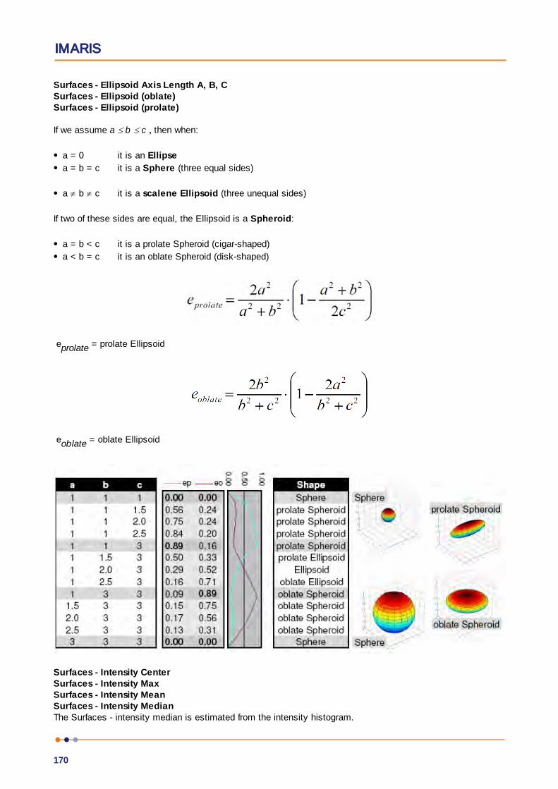
http://en.wikipedia.org/wiki/Moment_of_inertia#Principal_moments_of_inertia

IMARIS

170

Surfaces - Ellipsoid Axis Length A, B, CSurfaces - Ellipsoid (oblate)Surfaces - Ellipsoid (prolate)

If we assume a b c , then when:







eprolate = prolate Ellipsoid

eoblate = oblate Ellipsoid

Surfaces - Intensity CenterSurfaces - Intensity MaxSurfaces - Intensity MeanSurfaces - Intensity MedianThe Surfaces - intensity median is estimated from the intensity histogram.

Reference Manual

171

Surfaces - Intensity MinSurfaces - Intensity StdDevSurfaces - Intensity SumThe voxel intensity statistics describe the voxels enclosed within the Surfaces (Center, Max, Mean, Median,


Surface- Number of Disconnected Components

The number of disconnected surfaces in the selected Surface object.

Surface- Number of Disconnected Components per Time Point

The number of created disconnected surfaces in the selected time point.

Surfaces - Number of Surfaces per Time PointNumber of Surfaces per actual Time Point.

Surfaces - Number of TracksNumber of tracks.

Surfaces - Number of TrianglesNumber of the Surface object triangles.

Surfaces - Number of VerticesNumber of the Surface object vertices.

Surfaces - Number of VoxelsNumber of voxels within the selected Surface object.

Surfaces - Position X, Y, Z The X, Y and Z coordinates of the surface object. The value is equal to the value of the Center of Homogeneous

Mass of the object.

Surfaces - SpeedThe surfaces speed is the instantaneous speed of the object (um/s).The instantaneous speed is the scalar


Surface - SphericitySphericity is a measure of how spherical an object is. Defined by Wadell in 1932, the sphericity, , of a particle

is the ratio of the surface area of a sphere (with the same volume as the given particle) to the surface area of

the particle:

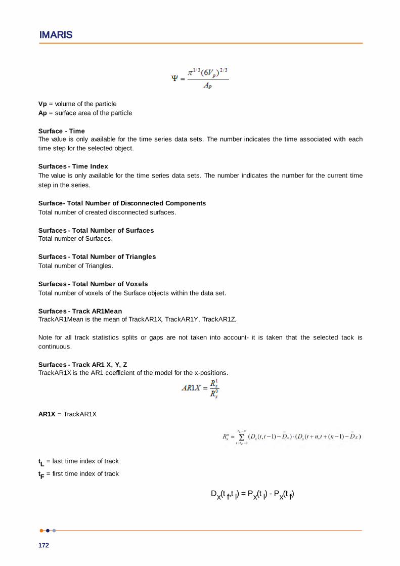
IMARIS

172



Surface - Time The value is only available for the time series data sets. The number indicates the time associated with each


Surfaces - Time Index


step in the series.

Surface- Total Number of Disconnected Components

Total number of created disconnected surfaces.

Surfaces - Total Number of SurfacesTotal number of Surfaces.

Surfaces - Total Number of Triangles

Total number of Triangles.

Surfaces - Total Number of Voxels

Total number of voxels of the Surface objects within the data set.

Surfaces - Track AR1MeanTrackAR1Mean is the mean of TrackAR1X, TrackAR1Y, TrackAR1Z.

Note for all track statistics splits or gaps are not taken into account- it is taken that the selected tack is

continuous.

Surfaces - Track AR1 X, Y, ZTrackAR1X is the AR1 coefficient of the model for the x-positions.

AR1X = TrackAR1X




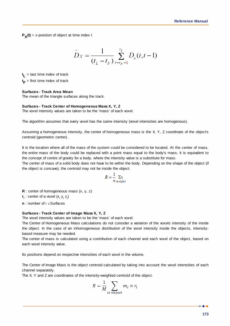
Reference Manual

173




Surfaces - Track Area MeanThe mean of the triangle surfaces along the track.

Surfaces - Track Center of Homogeneous Mass X, Y, ZThe voxel intensity values are taken to be the ‘mass’ of each voxel.











i z

i)


Surfaces - Track Center of Image Mass X, Y, ZThe voxel intensity values are taken to be the ‘mass’ of each voxel.








channel separately.


IMARIS

174




i z

i)


Surfaces -Track Displacement X, Y and ZThe object’s Track Displacement is the distance between the first and last object’s position along the selected-

axis:

Surfaces - Track Displacement Length


Surfaces - Displacement Delta XYZ


Surfaces - Displacement Delta Length (a scalar value)


Surfaces - Track DurationThe Track Duration is the duration between the first and last time point within the Track.

Surfaces - Track Ellipsoid Axis A X, Y, Z MeanThese three parameters define the Vector of the track Ellipsoid Axis a.

Surfaces - Track Ellipsoid Axis B X, Y, Z MeanThese three parameters define the Vector of the track Ellipsoid Axis b.

Surfaces - Track Ellipsoid Axis C X, Y, Z MeanThese three parameters define the Vector of the track Ellipsoid Axis c.

Surfaces - Track Ellipsoid Axis Length A, B, C MeanThese three parameters define the length of the Ellipsoid Axis a, b, and c.

Surfaces - Track Ellipsoid Oblate A MeanThis parameter defines the mean Ellipsoid Oblate for the track (see above for the detailed oblate definition).

Surfaces - Track Ellipsoid Prolate A MeanThis parameter defines the mean Ellipsoid Prolate for the track (see above for the detailed prolate definition).

Surfaces - Track Intensity Center MeanThis value describes the mean voxel intensity in the center of the Surfaces.

Surfaces - Track Intensity MaxThis is the maximum value of all maximum (voxel) intensities of the surface along the tracks

Surfaces - Track Intensity Mean

Reference Manual

175

This is the weighted mean of the objects means, equal to the simple mean of all the intensities of all theobjects in a track. Larger objects have a larger impact on the track mean.

Surfaces - Track Intensity MedianThe median intensity for a track is calculated as the (approximated) median of the (approximated) medians of


Surfaces - Track Intensity MinThis is the minimum value of all minimum (voxel) intensities of the surface along the tracks

Surfaces - Track Intensity StdDevThis value describes the Standard Deviation voxel intensity of the Surfaces along the tracks.

Surfaces - Track Intensity SumThis value describes the sum of voxel intensity of the Surfaces along the tracks. Surfaces - Track LengthThe Track Length is the total length of displacements within the Track.



Surfaces - Track Number of BranchesA branch occurs when a Surface object is connected to several other Surface objects of a future time point.

Surfaces - Track Number of FusionsA fusion occurs when a Surface object is connected to several Surface objects of a past time point.

Surfaces - Track Number of SurfacesThe total number of Surfaces along the track.

Surfaces - Track Number of TrianglesNumber of Triangles along the track.

Surfaces - Track Number of VoxelsNumber of Voxels along the track.

Surfaces - Track Position X, Y, Z MeanDefines the mean value of X, Y, Z track coordinates positions.

Surfaces - Tracks Position X, Y, Z Start


Surfaces - Track Speed Max, Mean, Min, StdDev Maximum, mean, minimum and standard deviation of the value of the object’s speed on the track.

Surfaces - Track Speed Variation



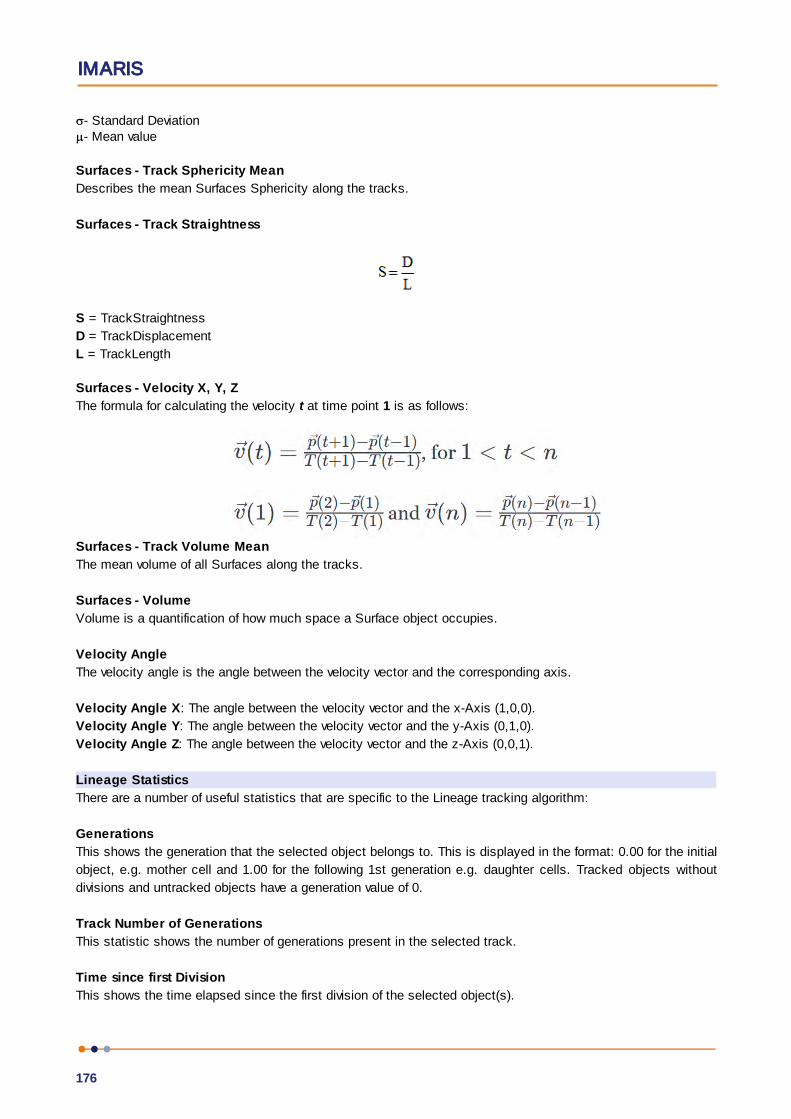
IMARIS

176


Surfaces - Track Sphericity Mean

Describes the mean Surfaces Sphericity along the tracks.

Surfaces - Track Straightness



L = TrackLength

Surfaces - Velocity X, Y, Z

The formula for calculating the velocity t at time point 1 is as follows:

Surfaces - Track Volume Mean

The mean volume of all Surfaces along the tracks.

Surfaces - Volume

Volume is a quantification of how much space a Surface object occupies.

Velocity Angle





Lineage Statistics


Generations








Reference Manual

177











the calculation.






Cell Cycle Duration









5.9.9.6 VolumeVolume statistics are automatically computed for each Volume object. These can be viewed from the statistics

tab.

Show Statistic Values - Volume

Volume - Data Intensity Mean

Volume - Data Intensity StdDev

Volume - Data Intensity Sum

The volume intensity statistics describe the voxels of the whole data set (Mean, StdDev and Sum).

Volume - Data Volume

The Data Volume is a quantification of how much space an object occupies.

Volume - Number of Voxels

Number of the Volume voxels.

5.9.10 Statistics Tests

The settings for the Statistics Tests calculated and displayed in the Statistics Tests tab of 1D view can be


IMARIS

178

viewed or edited as required.

Common Preferences

Set the Confidence level for all tests. The default is 0.05.

Wilcoxon Test

Select the type of test performed. Select between Two tails test (default), Left tail test or Right tail test.

F test


T Test


Select whether the assumption will be made that the original populations have the same variances. The default

is unselected- in this case a Student’s t-test is performed. If this option is selected, a Welch’s t-test will be

performed.

Kolmogorov-Smironov Test


5.9.11 Snapshot

Configure the preferences for Snapshot. Note that the default file format is tiff.

Save

Size

Adjust the size of the snapshot image. Select the image size either as that of the Window size or a Fixed

size. Set the Fixed size to a required resolution using the Width and Height fields.

Reference Manual

179

DPI

Adjust the print resolution of the snapshot image. The default value is 300dpi. This can be increased for higher

resolution, or decreased if required.

Save as type

Select the file format: TIFF (default), PNG and JPEG).

Copy to Clipboard

Set the snapshot image to save to clipboard e.g. so the image may be pasted into a document. Note this mode

of copying will not support transparent backgrounds.

Save to File

Set Save to file to save the snapshot image directly to filethis will save the image directly to the set image

output directory so that multiple snapshot image may be taken quickly and easily.

Transparent Background

Save images so that the background of the image is transparent.

Open Saved File in Default Image Viewer

Selecting this option will result in the snapshot image opening automatically in your default image browser.

Image Output Directory

Set your preferred save location options for Snapshot images.

Source Image Directory

Not available when Imaris has been configured for Arena (Arena is the default, recommended option)- this option

enables snapshot images to be saved to the source image directory location.

Always Prompt User

Select this option to always prompt the save location each time you take a snapshot image.

Custom

Imaris will use a logical location by default to save snapshot files to, but you can change this to a more suitable

location if required. The current location is shown and the Browse button can be used to set a new location

Open Output Directory Button

Open the set output directory to new the folder contents.

Load and Save Window State

Custom settings can be saved as a window state- these may be saved and loaded from the View menu options:

Load Window State and Save Window State.

5.9.12 Custom Tools

ImageJ / Fiji Application

The Browse button allows you to browse to a desired location within the file system.

Here you can specify the Fiji folder in which the Fiji.exe file resides. Either type in the respective path or use

the button Browse.

Please note: Fiji can be downloaded from the Bitplane Customer Portal.

http://portal.bitplane.com/


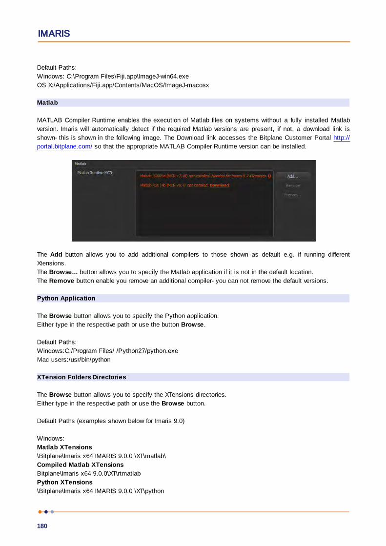
IMARIS

180

Default Paths:

Windows: C:\Program Files\Fiji.app\ImageJ-win64.exe

OS X:/Applications/Fiji.app/Contents/MacOS/ImageJ-macosx

Matlab

MATLAB Compiler Runtime enables the execution of Matlab files on systems without a fully installed Matlab

version. Imaris will automatically detect if the required Matlab versions are present, if not, a download link is

shown- this is shown in the following image. The Download link accesses the Bitplane Customer Portal http://

portal.bitplane.com/ so that the appropriate MATLAB Compiler Runtime version can be installed.

The Add button allows you to add additional compilers to those shown as default e.g. if running different

Xtensions.

The Browse... button allows you to specify the Matlab application if it is not in the default location.

The Remove button enable you remove an additional compiler- you can not remove the default versions.

Python Application

The Browse button allows you to specify the Python application.

Either type in the respective path or use the button Browse.

Default Paths:

Windows:C:/Program Files/ /Python27/python.exe

Mac users:/usr/bin/python

XTension Folders Directories

The Browse button allows you to specify the XTensions directories.

Either type in the respective path or use the Browse button.

Default Paths (examples shown below for Imaris 9.0)

Windows:

Matlab XTensions

\Bitplane\Imaris x64 IMARIS 9.0.0 \XT\matlab\

Compiled Matlab XTensions

Bitplane\Imaris x64 9.0.0\XT\rtmatlab

Python XTensions

\Bitplane\Imaris x64 IMARIS 9.0.0 \XT\python



Reference Manual

181

OS X

Matlab XTensions

/Applications/Imaris IMARIS 9.0.app/Contents/SharedSupport/XT/matlab

Compiled Matlab XTensions

/Applications/Imaris IMARIS 9.0.app/Contents/SharedSupport/XT/rtmatlab

Python XTensions

/Applications/Imaris IMARIS 9.0.app/Contents/SharedSupport/XT/python

Please note: Fiji and MATLAB Compiler Runtime can be downloaded from the Bitplane Customer Portal.

MATLAB Compiler Runtime enables the execution of Matlab files on systems without a fully installed Matlab

version.


Add Button

To add a XTensions directory, click on the Add button.

Remove Button

Click on the Remove button to remove the selected XTensions directory from the list.

OK Button


Cancel Button


5.9.13 Licenses

Overview

Node-locked License

Node-locked licenses grant permission to run the licensed software on one computer (node) only. Node-locked

licenses are the easiest way to license the software. You can use the Imaris Administrator to directly download

a node-locked license from the Bitplane server. If your computer is not connected to the Internet it is also

possible to download this license from another computer and then copy it to the target machine. Please refer to

the offline license method for further instructions.

Floating License

Floating licenses grant permission to run the licensed software on several computers. One floating license can

activate only one instance of the program at any given time. Floating licenses require the installation of a

separate license server that runs on a Windows computer. The server installation requires more technical know

how.

The Imaris Administrator application easily let you enable a floating license.

Demo License

A Demo License is a time-limited (usually one month) license. It is not an official licensing scheme and

therefore can't be purchased. It's main purpose is for internal Testing and to grant customers with licensing

issues an easy and quick workaround so that their productivity can continue until the problem is solved. Simply

open the Imaris Administrator application and open the Demo License you received from your local support

representative.

Evaluation License


IMARIS

182

Evaluation Licenses are temporary licenses allowing customers to explore all fascinating possibilities Imaris

offers before actually purchasing it. The license is only limited in time (10 days), but not in features. Additionally

an Evaluation License is issued per user.

To get an Evaluation License you first have to register at:

http://www.bitplane.com/go/download/imaris-evaluation

An automatic mail response should provide you with your personal RegistrationID and its corresponding

Passcode. These credentials can then be entered during the application's start up.

Imaris Open Developer License

To get an Imaris Open Developer License you first have to register at:

http://open.bitplane.com/

If you can install multiple license locations, (Floating license and a Node-Locked license), Imaris will search all

the locations until it finds the license for the requested features.

This Section contains information related to licensing management, options and procedures. It includes the

following sections:

Preferences Dialog

Installation of Licenses

Imaris Administrator

5.9.13.1 Preferences DialogImaris Administrator enables the licenses of various Bitplane applications (and Imaris data and system

settings) to be managed by the Administrator. It provides a simple interface to add or delete any licenses.

When a license is added, the license file gets copied to a system folder where it is secure from (accidental)

manipulation by standard users. Although it is possible for administrators to modify license files directly in this

system folder we strongly advise you not to do so. It is recommended to go through the Imaris Administrator

application instead.


This starts the Imaris Administrator. Unless you want to use an Evaluation license you need to use the Imaris

Administrator to set up your licenses.

Please note that you'll need administrative privileges in order to start the Imaris Administrator.

Any change of licenses will require Imaris to be restarted.

Except the Evaluation License which is bound to a single user, all other licenses are bound to the whole

system. Therefore any license modifications need administrative privileges.

If you have access to an administrative system account, Imaris Administrator will start normally.

Administrate

This button starts Imaris Administrator. This is a tool shipped with Imaris in order to add or modify licenses.

Unless you want to use an Evaluation license you need to use Imaris Administrator to set up your licenses.

Please note that you'll need administrative privileges in order to start Imaris Administrator.

Any change of licenses will require a new start of Imaris.


Reference Manual

183

Evaluation License

After you entered your RegistrationID and Passcode you can click on the Light Bulb button to activate the

Evaluation License.

This action requires an internet connection because the licenses are downloaded directly from the Bitplane

server. Upon success, the light bulb will turn on .

You can also disable your Evaluation License by clicking again on Light Bulb button and the light bulb will turn

off. This indicates that you aren't using any Evaluation Licenses.


RegistrationIDPlease enter your RegistrationID you received by mail previously.

PasscodePlease enter your Passcode you received by mail previously.


After you entered your OrderID click on the Imaris Open button to activate the Developer License.


server. Upon success, the button will turn on .


RegistrationIDPlease enter your RegistrationID you received by mail first.

Available Licenses

The table displays all existing Imaris licenses on the system and additional information for each feature:

Version

The latest Imaris version this license can be used with.

Type

Which type of licensing scheme is used. An overview is given in the Licenses section.

Status

Displays the status of a license.

Expiration

Shows the number of days until this license expires.

License colors

In order to gain a quick overview, the validity of a license is also indicated by different colors:

Green: License is valid.

Yellow: License is valid, but all licenses are currently in use.

Red: License has expired.

No color: License is not available (e.g. this additional license feature hasn't been purchased).

You can select with which license(s) your Imaris should start per default. Any change will require a new start of

IMARIS

184

Imaris.

Check/Uncheck All

Check this box to enable or disable all available Imaris licenses on the system.

Please note that the Feature “ImarisBase” can't be disabled because this would render Imaris unusable.

5.9.13.2 Installation of LicensesFirst-time Installation

If you have installed Imaris for the very first time, you have to set up a license before you can use Imaris.

A dialog window appears during the start up of the application.

The same dialog window appears if you have accidentally deleted the license .

You now have two options how to proceed:

• If you have a Node-locked or a Floating License you should use Imaris Administrator application for the further

license setup. This is done by simply clicking on the “Start Imaris Administrator” button. Please note that

Imaris Administrator application needs administrative privileges.

• If you want to evaluate Imaris first, please register at:


The automatic mail response contains your Registration ID and Passcode.

To enable an Evaluation License enter these values in the corresponding fields and click on the “Use Evaluation

License” button.

Please note that a working internet connection is needed to start up Imaris in Evaluation mode.

Installation of Additional Licenses

If you already have set up a license but you want to add other licenses as well, you can do this in the License

Preferences dialog.

Once more, you'll have the option either to start Imaris Administrator application or to use an Evaluation

License in addition if you would like to try out a new feature before buying the license.

5.9.14 Update

Here you can adjust the default update settings.

How often should you search for updates?

Daily

Weekly

Never

Select either daily, weekly, or never.

Button OK



Reference Manual

185

Button Cancel


5.9.15 Usage Data

Here you can enable the capturing of data usage.

Button OK


Button Cancel


5.9.16 3D Cursor

Here you can adjust the default 3D Cursor settings.

3D Cursor

Box

Sphere

Cross

Torus

Here you can select the shape of the 3D Cursor.

Size

Color

Here you can select the size and color of the 3D Cursor.

Animation

Frequency

Adjust the animation frequency.

Amplitude X

Amplitude Y

Adjust the amplitude in x-, and y-direction.

Shear

Rotate

Select shear or rotate as animation mode.

Continuous

Discrete

Select continuous or discrete as animation sequence.

Button OK

IMARIS

186


Button Cancel


5.9.17 Annotate

Here you can adjust the default Annotation settings.

Format

Title Format

Text Format

Legend Format

Choose title format, text format or legend format and adjust the following parameter set.

Title, Text or Legend

Font

Font Size

Color

Format

Bold

Italic

Underlined

The font, font size, color, and format can be selected (from any installed system font).

Color Selection Button


Style

Arrow Color

Arrow Width

Arrow Style

Text Box Color

Text Box Transparency

Text Box Style

You can adjust the arrow color, width and style (Sphere, Arrow, Magnifier), text box color, transparency and

style (Unicolor, Black Text, Black Title).

Color Selection Button


Button OK


Button Cancel


Reference Manual

187

5.9.18 Arena

Change the default storage location for image data sets from the Arena menu of Preferences. This can be either

a local drive or remote location e.g. a network server enabling access to files across a network.

If Imaris detects existing data at the new location it will use this data and not overwrite it. If it doesn't detect

existing data it will copy the data from the previous storage location.

To see how to modify the Arena Storage location refer to Modify Arena Storage Location.

Notes:

Imaris file server authentication is a secure form of authentication because a hashed version of the

password and user name are sent in a cryptographic exchange with the server.

Imaris 8.3 onwards supports the SMB application layer network protocol which is the default

protocol on Microsoft Windows OS and supported by Apple OSX.

Using Remote Data Storage Locations

When using a Remote Share location to store data sets you must enter authentication credentials to enable

access and sharing of files.

Enter your credentials: a user name and password, when required.

When an incorrect user name or password is used, please retype your credentials and try again.

Then click OK to continue.

Remote Share locations that have been set-up are listed under Store. Use the Edit and Delete buttons to

manage the Remote Share locations for images.

5.9.18.1 Modify Arena Storage LocationChanging the Data Storage Location

To change the storage location proceed as follows:

1. Click Modify Storage Location.

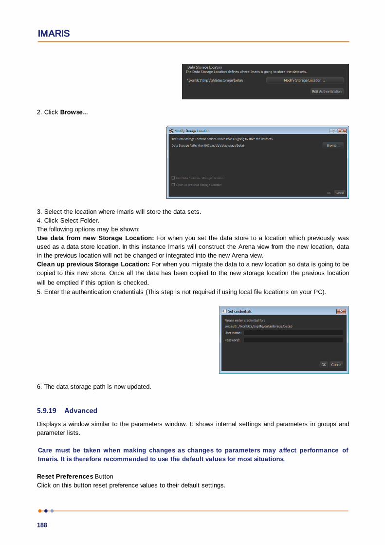
IMARIS

188

2. Click Browse...

3. Select the location where Imaris will store the data sets.

4. Click Select Folder.

The following options may be shown:

Use data from new Storage Location: For when you set the data store to a location which previously was

used as a data store location. In this instance Imaris will construct the Arena view from the new location, data

in the previous location will not be changed or integrated into the new Arena view.

Clean up previous Storage Location: For when you migrate the data to a new location so data is going to be

copied to this new store. Once all the data has been copied to the new storage location the previous location

will be emptied if this option is checked.5. Enter the authentication credentials (This step is not required if using local file locations on your PC).

6. The data storage path is now updated.

5.9.19 Advanced

Displays a window similar to the parameters window. It shows internal settings and parameters in groups and

parameter lists.

Care must be taken when making changes as changes to parameters may affect performance of

Imaris. It is therefore recommended to use the default values for most situations.

Reset Preferences Button

Click on this button reset preference values to their default settings.

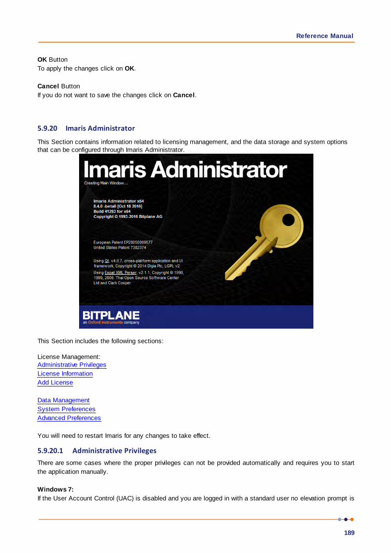
Reference Manual

189

OK Button


Cancel Button


5.9.20 Imaris Administrator

This Section contains information related to licensing management, and the data storage and system optionsthat can be configured through Imaris Administrator.

This Section includes the following sections:

License Management:Administrative Privileges

License Information

Add License

Data Management

System Preferences

Advanced Preferences

You will need to restart Imaris for any changes to take effect.

5.9.20.1 Administrative PrivilegesThere are some cases where the proper privileges can not be provided automatically and requires you to start

the application manually.

Windows 7:

If the User Account Control (UAC) is disabled and you are logged in with a standard user no elevation prompt is

IMARIS

190

shown because the UAC setting omits these prompts. Therefore you can't get the right administrative

permissions and you will have to start Imaris Administrator manually. This is done by opening the executable

by a right click while holding down the “Shift” key. Then you can select “Run as different User” which prompts

you for another account.

Mac OS X:

No cases known where problems occur.

Default Imaris Administrator Paths

Windows 7, 8 and 10

64-bit: C:\Program Files\Bitplane\Imaris 9.0\ImarisAdministrator.exe

Mac OS X

/Applications/Imaris 9.0.app/Contents/MacOS/ImarisAdministrator

5.9.20.2 License InformationTypes of license

A description of the license types available is given in the Licenses Section.

License Location

If you did not have set up a license yet (e.g. first-time usage) this window is empty. In that case, please use

the Add License Location button to add a new license location.

Add License Location Button

Use this button to add new licenses. A description is given in the Add License Section.

Delete License Location

If you click this button, the selected license location entry in the table underneath will be deleted. Before using

this button, please make sure you have selected the right table entry. In the case of a node-locked license, you

are asked if you want to keep the license. It is recommended that you keep all license files.

License Location Table

This table lists all available license locations. Normally it would be just enough to have one license location

defined. But there are also situations in which it is useful to use multiple locations.

For example you might have a floating license server with just some basic features enabled. Maybe later you

purchased some additional features in a node-locked licensing scheme. You can now just define both locations

and the licensed features are merged on your system automatically.

The table shows also some additional Information:

• Type: This is either a License Server (floating license scheme) or a License File (all other schemes)

• Number of valid / total Licenses: These numbers show you how many different features your license contains

and it lets you easily verify that all licenses are still valid.

If you click on another table entry, the License table underneath gets updated and shows you detailed

information about all available features of the current selected license location.

Licenses Table

Reference Manual

191

In this table you have a detailed overview of all licensed features of a license location. You can switch among

different license locations by selecting the corresponding entry in the License Location table.

Each feature provides some information :

Version


Type

Which type of licensing scheme is used. An overview is given in the Licenses section.

Status


Expiration


License colors


Green: License is valid.

Yellow: License is valid, but all licenses are currently in use.

Red: License has expired.

No color: License is not available (e.g. this additional license feature hasn't been purchased).

Finish Button

This button is only enabled if you have added at least one license location. It is an indicator when all necessary

steps to set up a license are done. If all features in the above License table are highlighted in green (or only

some of them) you successfully managed to add a license. If you click the button, it just closes Imaris

Administrator and you can proceed using Imaris.

5.9.20.3 Add LicenseFirst, you have to select your licensing scheme:

Download Node-locked License

If you decide to add a Node-locked License, the software will verify that your computer is connected to the

internet. If the connection could be established successfully, the Online-Licensing Wizard is shown; if not, you

have the possibility to download the license from another computer which is described in the Offline-Licensing

Wizard.

Online-Licensing Wizard

This wizard has three steps:

1. Select the Network Interface

You need to select the network interface which is bound to the license. If your Host-ID is already known to our

server, the available product for installation will be shown in the table below.

2. Check your Order-ID for newly ordered Products:

If you have ordered new products, you have to enter the Order-ID in this step. Clicking on the “Check Order-ID”

button will add the products to the table below. Once you checked an Order-ID, it is bound to the currently

selected network interface.

If your Host-ID is already known to the system, the available products will be shown in the tables below and you

could skip that step.

3. Select the Licenses for Installation

In this step you just have to mark all products you want to install by checking them in the left table.

IMARIS

192

The right table is for your information only and shows all currently installed products.

When you click on the “OK” button, the license file is downloaded and the corresponding entry is added to the

License Location table.

Offline-Licensing Wizard

If you are not connected to the Internet, this could be due to either of the following:

1. your computer is behind a web proxy server which does not permit a direct connection or

2. the PC is unplugged from the internet.

Therefore you have the following choices:

A) Set up a Proxy Server

Enter your proxy server's name and its port and click on the Test Connection button. If the connection could

be established you are automatically redirected to the Online-Licensing Wizard described above.

If not, either the credentials you entered are not correct or the connection is broken at another place in the

network. In that case please contact your network administrator or Bitplane Support teams

[email protected] or

[email protected]

If you want to delete a previously set up proxy server, just delete both fields and click on the button again.

The proxy server settings can also be altered in Imaris' system preferences dialog.

B) Download the Node-locked License from another Computer

You can download the license from another computer connected to the internet.

On that machine log on to http://www.bitplane.com/activation/acti_offline_ident.html

and enter the Host-ID you wish to bind to the license together with your Order-ID into the web form. The

download of the license should immediately start and afterwards you could transfer the file to the offline

computer (e.g. by using a USB stick).

The instructions can be saved in a file by clicking the Save Instructions... button.

When you have downloaded the license you can just open it with the Open License... button or enter its path

directly into the field on the left of the button.

When you click OK the license file is copied to the proper location.

Define Floating License Server

In order to add a Floating License Server, just enter the server's name and its port to the corresponding fields

and click on the OK button. The default port is 2700.

Install License from Existing File

If you received a Demo License from your local support representative or you need to add a license file directly

you can use this wizard. If you click on the Open License... button you can browse to the license you want to

add. You can also specify the license file to load by entering its path directly into the field left from the button. If

you click on the OK button, the license is copied to the right location and it's added to your License Location

table.

Show floating license selection dialog upon start of Imaris

This option enables you to enforce active individual selection of all Imaris add-on modules licenses and secure

the optimal use of the licenses available on the server. It prevents unintentionally overuse of the purchased add-



http://www.bitplane.com/activation/acti_offline_ident.html


Reference Manual

193

on modules licenses and helps you with your short- and long-term plans for Imaris licenses spending and

allows you to better control your software cost.

Select the Show floating license selection dialog upon start of Imaris and you are configuring the License

Selection table to starts automatically. So every time Imaris is started Imaris, the License Selection table is

displayed for each user.

5.9.20.4 License SelectionIt is important to understand that the License Selection option is not designed to minimize your Imaris usage. It

lets you manage and optimize use of all Imaris add-on modules licenses that are available within your license

purchased pool.

When you launch Imaris, the License Selection table will be shown. With the License Selection table the user

has the flexibility to mix and match add-on modules and to suit changing scientific requirements in a flexible

form. The License Selection table allows selection of all add-on Imaris modules to be simultaneous used by

any number of users up to the maximum number of licenses agreed upon at the time of purchase.

The table displays only the Imaris add-on module license that does not match the overall number of purchased

Imaris basic licenses.

This table displays: Imaris product, feature, version, license type and status and expiration date.

From the modules lists, you can select the required license.

Choose from the table the modules that are needed and available and select only the add-on modules that will

be needed for the current Imaris session. Activate your license by clicking the appropriate check-box.

After activating the license, for the selected module the total license number available in the pool is reduced.

Once all available licenses are checked out (the activated license number has been exceeded the maximal

number of license have been purchased), the corresponding Imaris product will not be shown within the table.

The product will not be available for your future selection until one of the current users is finished and the

license is checked back into the licensing pool.

Do not show this dialog

If you select this option, you won’t have a license table opened on your system, and the opt-in licenses file will

not be available for your future selection.

5.9.20.5 Data ManagementThe administrator can set the default location that the data set and batch data files are saved to using Set Data

Storage Path. This can be either a local, or a remote network server location. This is described in the Arena

Section. The user can change the default location if they require.

5.9.20.6 System PreferencesSystem Preferences allows an administrator to set the key system parameters for Imaris users. Default values

are detected for the computer by the software and automatically set in the Number of Threads, Data Cache

Memory Limit and Texture Cache Limits fields. These values can be set manually if required by free typing or

using the up and down arrows in each field.

System Preferences are set by default so they are editable by the user. This can be disabled by deselecting

the Is editable by User check-box.

Select Reset to Factory Defaults to change any modified values back to the original default values. Click the

Finish button when you are finished making changes. You will need to restart Imaris for any changes to take

effect.

IMARIS

194

Care must be taken when making changes as changes to parameters may affect performance of Imaris. It is

therefore recommended to use the default values for most situations. Refer also to the Calculation Section.

Calculation

The number of processing threads can be adjusted from the default value depending on the system resource

requirements of the computer running Imaris.

Data Cache

Adjust the size of the Data Cache Memory Limit and set and select the Data Cache File Path to be used.

Display

Set the maximum memory limit allocated to the texture cache used for display. Adjusting the Texture Cache

Limit can be used to improve image quality or performance or according to the size of the images and the

computer resources available.

Settings

Set the frequency for maintenance and and software updates. The default setting is Weekly.

Usage Data

Enable or disable the capturing of usage data. Refer also to the Usage Data Section.

5.9.20.7 Advanced PreferencesIn Advanced Preferences it is possible to edit parameters in Imaris and set whether they may be editable by the

user under the Advanced option of preferences. Care must be taken when making changes as changes to

parameters may affect performance of Imaris. It is therefore recommended to use the default values for most

situations. To return values to the original default values select Reset to Factory Defaults. Click the Finish

button when you are finished making changes. You will need to restart Imaris for any changes to take effect.

5.10 ExitTerminates Imaris and returns to the desktop.

Reference Manual

195

Section 6 Edit

Undo Ctrl + Z

Snapshot Ctrl + C

Image Properties... Ctrl + I

Show Display Adjustment Ctrl + D

Annotate Ctrl + Shift + P

Add Time Points...

Delete Time Points...

Add Channels... Ctrl + Shift + A

Delete Channels... Ctrl + Shift + B

Add Slices...

Delete Slices...

Remove images

Crop Time...

Resample Time...

Crop 3D... Ctrl + W

Resample 3D...

Change Data Type...

File Type Associations...

See also:


6.1 UndoThe Undo command reverses the last action, when necessary. It supports multiple undo actions, starting withthe most recent one and working backwards in sequence.

All actions in the Draw , Edit and Edit Tracks tabs as well as the image processing functions can be

undone by selecting the Undo command or by pressing Ctrl+Z.

The number of any previously applied command that can be Undone/Redone is defined in the Edit menu-

Preferences-Calculations-Maximum Number of Commands in History field. By default, the number of steps

is 4.

6.2 RedoThe Redo command repeats the last action, if appropriate. The command supports multiple redo actions,

starting with the most recent one and working backwards in sequence.

All action in the Edit, Edit tracks, and Draw tabs as well as image processing functions can be redone by

selecting the Redo command or by pressing Ctrl+Y.

The number of any previously applied command that can be Undo/Redo is defined in the Edit menu-

Preferences-Calculations-Maximum Number of Commands in History field.

IMARIS

196

6.3 SnapshotThe snapshot button in the main toolbar immediately produces a snapshot of the current view. This may be

either the image is Surpass, or a 2D, 3D or 4D Vantage plot as it currently appears in the viewing area. It

creates a new file containing your Vantage plot as well any scale information, measurements data, and box

plots that are displayed.

By default the snapshot is saved to a file in the source image directory and after creating the snapshot it is

opened in the default image viewer to show the user what the snapshot looks like. The snapshot is by default

also copied to the operating system clipboard for use in other applications.

To create the snapshot, simply click the Snapshot button.

To view and adjust the settings of the snapshot, click Preferences from the Snapshot button drop-down box.

Refer to Snapshot Preferences for further information.

Notes:

To help the user see the size of the screen render area, Imaris displays this size in the top left

hand corner of the render-area whenever the size is changed (shown below).

The view-menu has “Save Window State” and “Load Window State” options which function on a

per viewer basis, to save and load the size and visibility of all windows.

Snapshots always have the same aspect ratio as the render-area of the current view. (In previous

versions of Imaris it was possible to create snapshots with aspect ratios differing from those of the

current view).

6.4 Image Properties...Geometry

Data Set

Channels

(Channel 1...n)

Thumbnail

Parameters

When opening a data set, the following parameters should be checked or modified as required:

Name and Description (in Data Set).

Voxel Sizes (in Geometry).

Channel Colors (in Channel 1...n).

Reference Manual

197

6.4.1 Geometry

The geometrical settings of the actual data set are displayed.

Type

Data Type

Display of the image type.

Size

Size X, Y, Z, T

Display of the image size.

Image size:

Shows the uncompressed image size.

Coordinates (um)

Voxel Size, X, Y, Z

The voxel sizes directly influence the views because they control the height of the image relative to its width.

Check the parameters and adjust the Voxel Size and/or other settings if necessary.

Min, X, Y, Z

The minimum value of the coordinate axes.

Max, X, Y, Z

The maximum value of the coordinate axes.

Time Point

First Box

Select the time point.

Date

Enter the collection data.

Time

Enter the collection time.

Button All Equidistant...

If the data set is a time series, enter the date/time for each time point or click All Equidistant to open the Set

Equidistant Time Points dialog box.

Enter the Start Date and Start Time and the Time Interval.

Click OK when finished. Imaris will calculate the time for each time point in the series.

The data set must be saved to retain the changes. Click OK when finished or select another heading for further

adjustments.

IMARIS

198

Button OK


Button Cancel


6.4.2 Data Set

Name

Data field to enter a data set name.

Description

Data field to enter a data set description.

Numerical Aperture (N.A.)

Reads out the numerical aperture (as defined in the menu Edit - Image Properties... - Parameters).

Log

Display of processing steps.

Button OK


Button Cancel


6.4.3 Channels

There are no parameters available on this menu.

6.4.4 Channel 1...n

In the Index of the Image Properties box click the Channel entry (Channel 1, Channel 2 etc.) to select the

required channel.

Name

Data field to type in the channel name.

Description

Data field to type in a channel description.

Reference Manual

199

Emission Wavelength

Reads out the emission wavelength.

Excitation Wavelength

Reads out the excitation wavelength.

Pinhole Radius

Reads out the pinhole radius.

Button OK


Button Cancel


6.4.4.1 Tab Base ColorRed, Green, Blue

Reads out the assigned color. To change the color either adjust the values or move the square in the color

circle.


6.4.4.2 Tab Mapped ColorSelected Color

Button Edit...

Click on a square in the grid and click on the button Edit... . Select a color and click on OK. The selected color

is displayed in the square.

Button Copy

Click on a square in the grid and then on the button Copy to copy the color.

Button Paste

Click on a square in the grid and then on the button Paste to paste the color.

Interpolation

Colorspace

RGB

The RGB color model is an additive model in which red, green and blue are combined in various ways to

reproduce other colors.

HSV

IMARIS

200

The HSV (Hue, Saturation, Value) model, defines a color space in terms of three constituent components.

Hue, the color type.

Saturation, the vibrancy of the color.

Value, the brightness of the color.

Button Interpolate

Select two squares in the grid and click on the button Interpolate. The colors between the two selected

squares are interpolated.

Color Table File

Button Import ...

Imaris comes with a set of pre-defined color tables. Click on Import... to open the Import Color Table File

window. Select a color table file and click on OK.

Button Export...

Click on the button Export... to open the Export Color Table File window. Select a destination and click on

Save.

A large number of predefined colormaps are available. If the default colormap (Spectrum) is not appropriate for

your application, you can change it by clicking on the drop-down list. The list gives a preview of what different

colormaps look like.


6.4.4.3 Tab Coloc StatisticsThe tab Coloc Statistics is available when a data set contains a Coloc channel and the Coloc channel is

selected in the channel selection of the Image Properties.

All statistics about the resulting colocalized volume are displayed. Definitions of the displayed values and

further information are given in Section Coloc - Volume Statistics.

Button Export...

Click on the button Export... to open the Export Color Table File window. Select a destination and click on

Save.

See also:


6.4.5 Thumbnail

Type

None

Select None if no thumbnail should be displayed.

Middle Slice

Thumbnail is the middle slice.

Reference Manual

201

MIP

Thumbnail in the display mode Maximum Intensity Projection. A Maximum Intensity Projection is a computer

visualization method for 3D data that projects in the visualization plane the voxels with maximum intensity that

fall in the way of parallel rays traced from the viewpoint to the plane of projection.

Blend

Thumbnail in blend projection. Blends all values along the viewing direction and includes their transparency.

Preview

Displays a preview of the thumbnail image.

Button OK


Button Cancel


6.4.6 Parameters

A set of informational parameters is appended to the image file.

Button Add Surpass Group...

Opens a dialog to add a new group.

Button Delete Surpass Group...

Deletes a Surpass group.

Button Add Parameter...

Opens a dialog to add a new parameter to the group.

Button Delete Parameter...

Deletes a parameter.

Button OK


Button Cancel


6.5 Show Display AdjustmentsThe Display Adjustment options let you choose the channel visibility as well as improve the image display by

concentrating on a limited color contrast range of voxels. Usually the color contrast values of the voxels stretch

over a wide range (e.g. 0 - 255).

The Display Adjustment function lets you set an upper limit for maximum color and a lower limit for minimum

IMARIS

202

color (i.e. black). The range between these two limits - represented by triangle symbols, is then extrapolated in

a linear mode to the full data set range and the new voxel values are calculated.

Display Adjustment Dialog (one for each channel)

Switch the individual channels on or off.

Check or uncheck the required channel check-box to switch the channel visibility.

Change the channel parameters such as name, color and description.

Click on the channel name to open the Image Properties. For a detailed description please refer to Section

Menu Edit - Image Properties - Channels 1...n.

Show/Hide all Channels

Check or uncheck to show or hide all channels as required.

Button Auto Adjust all Channels

The auto function works as follows: the minimum value is set to the first mode (maximum) of the histogram. The

maximum value is set to a value that is around the 99.8 percentile of the histogram which effectively disregards

high intensity outliers.

Reference Manual

203

Button Reset all Channels

Click on the button to set the image back to the original values.

Button Advanced

Click on the button to open the Advanced settings (see below).

Advanced Settings

Min

Max

Enter direct values in the Min (lower limit for minimum color) and Max (upper limit for maximum color) fields.

Alternatively drag in the display adjustment dialog the upper or lower handle of the adjustment line to adjust

the Min and Max limits.

The effect of the change can be seen on the channels (channels appear brighter or darker).

Gamma

The default value of the gamma correction is 1 (the range between lower and upper limit is extrapolated in a

linear mode to the full data set range). Enter a value below 1 and the linear mode is transferred to a nonlinear

mode, the lower intensities appear brighter. The effect of the change is directly visible in the viewing area.

Enter the value in the respective field.

Alternatively click onto the middle triangle in the display adjustment dialog and drag it to the left to increase

brightness/to the right to decrease brightness.

List of Shortcuts in the Display Adjustment Dialog

Please refer to Section Menu Edit - Show Display Adjustments - Mouse & Keyboard PC.

Please refer to Section Menu Edit - Show Display Adjustments - Mouse & Keyboard Mac.

Histogram

A histogram is a statistical data analysis, representing linear voxel within an image of the selected channel.

Change Channel Color

Click on the channel name to switch directly to the channel properties (Menu Edit - Image Properties -

Channels 1...n).

See also:

Menu Edit - Image Properties... - Channel 1...n

Menu Edit - Show Display Adjustments - Mouse & Keyboard PC

Menu Edit - Show Display Adjustments - Mouse & Keyboard Mac


Mouse & Keyboard Functions in the Display Adjustments Window

Ctrl + D Shows the Display Adjustment window

Left-click Select channel

Left-click on middle

triangle and drag

Adjust Gamma Correction

Ctrl + left-click Add channel to selection, or remove channel from selection

IMARIS

204

Left-click & drag Move left: make image channel brighter

Move right: make image channel darker

Move up: increase image channel contrast

Move down: decrease image channel contrast

Right-click & drag Move left: make image channel transparent

Move right: make image channel opaque

Ctrl + right-click Automatic range for Min and Max

See also:



Mouse & Keyboard Functions in the Display Adjustments Window

Command + D Shows the Display Adjustment window

Click Select channel

Left-click on middle triangle

and drag

Adjust Gamma Correction

Command + click Add channel to selection, or remove channel from selection

Click & drag Move left: make image channel brighter

Move right: make image channel darker

Move up: increase image channel contrast

Move down: decrease image channel contrast

ctrl + click & drag Move left: make image channel transparent

Move right: make image channel opaque

Command + ctrl + click Automatic range for Min and Max

See also:


6.6 Annotate

Annotate allows you to create figures of all Imaris views ready with the selected statistical values, titles,captions, labels, and other highlights for presentations or publications.

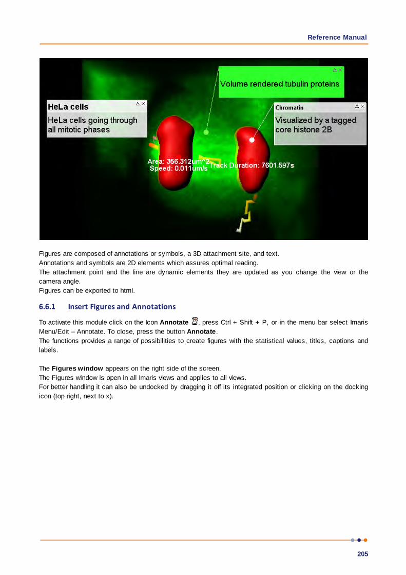
Reference Manual

205

Figures are composed of annotations or symbols, a 3D attachment site, and text.

Annotations and symbols are 2D elements which assures optimal reading.

The attachment point and the line are dynamic elements they are updated as you change the view or the

camera angle.

Figures can be exported to html.

6.6.1 Insert Figures and Annotations

To activate this module click on the Icon Annotate , press Ctrl + Shift + P, or in the menu bar select Imaris

Menu/Edit – Annotate. To close, press the button Annotate.

The functions provides a range of possibilities to create figures with the statistical values, titles, captions and

labels.

The Figures window appears on the right side of the screen.

The Figures window is open in all Imaris views and applies to all views.

For better handling it can also be undocked by dragging it off its integrated position or clicking on the docking

icon (top right, next to x).

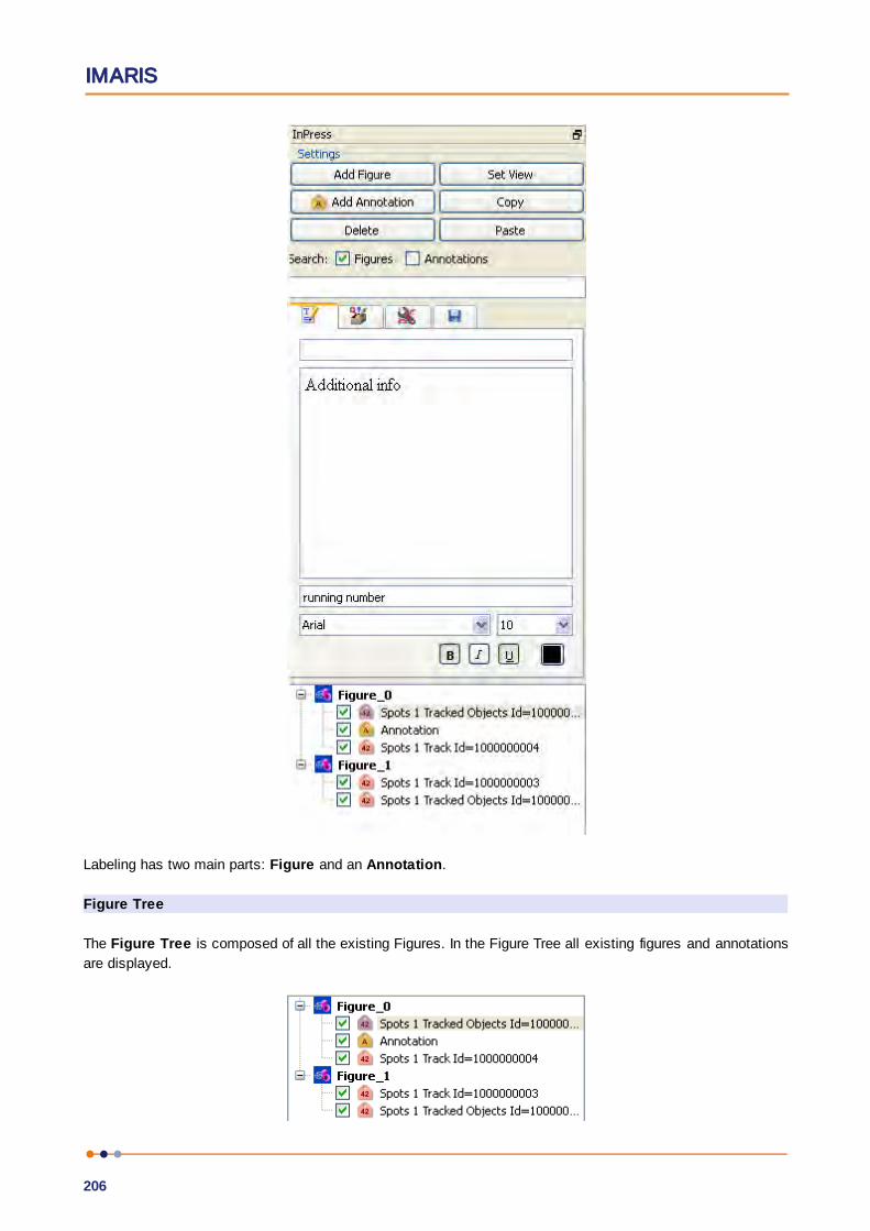
IMARIS

206

Labeling has two main parts: Figure and an Annotation.

Figure Tree

The Figure Tree is composed of all the existing Figures. In the Figure Tree all existing figures and annotations

are displayed.

Reference Manual

207

Within the selected Figure all the annotations’ names are displayed.

For a Figure, Imaris remembers the view that you were in and the camera position.

Annotations

The labels that are displayed in an image are called Annotations.In Imaris two types of the annotations exist:

Text annotation and Statistical annotation .

The Statistical annotation icon indicates the type of the selected statistical value and for that reason your

chose of the selected statistical value type will affect the appearance of the statistical annotation icon.

The following options are available:

Selecting a statistical variable that changes over time inserts the Statistical Annotation with the Time icon

in the selected Figure.

Selecting a statistical variable that is not time dependent inserts the Statistical Annotation icon in the

selected Figure.

Selecting or de-selecting the box next to the annotation name in the Figure Tree controls the visibility of the

annotation in the viewing area.

This Section also provides information on the following topics:

Annotation Box

Settings

Tab Text

Tab Style

Statistical Annotation

Tab Export

6.6.2 Annotation Box

Text Annotation

IMARIS

208

To create a Text annotation using the Setting options select the Add Annotation button

.

To create a Text annotation box, click in the image to set the 3D anchor point.

Move the mouse to elongate the line. With the second click you fix the top left corner of the text box.

Move the mouse to adjust the text box size. With the third click you fix the text box size.

Statistical Annotations

By default, statistical annotations are presented in the viewing area without an annotation box. To create the

annotation box for the statistical annotations select the annotation in the Figure Tree, and then activate the

Text box option under the Style tab .

The position of the statistical annotations can be adjusted by moving the annotation box and the anchor area.

The statistical annotation is assigned to the selected objects in the image and the anchor point

cannot be placed on another object.

Once created the annotation box and anchor point can be moved to the preferred location.

Move Annotation Point, Box, Number

To move the 3D anchor point set the mouse over the anchor point (until it changes to a cross) then click &

drag to a new location.

To move the annotation box set the mouse on the upper region of the box (until it changes to a cross) then

click & drag to a new location.

To move the annotation number set the mouse over it (until it changes to a cross) then click & drag to a new

location.

Resize the Annotation Box

To resize the annotation box set the mouse to an edge of the box (until the mouse changes to a resize icon)

and then click & drag the edge.

Annotation Visibility

The description area of the annotation can be closed (hidden) or expanded (shown) by clicking the triangle on

the top right of any annotation box.

The annotation can be hidden by clicking the “X” on the top right corner of the box.

Selecting or de-selecting the box next to the annotation name in the Figure tree controls the visibility of the

annotation in the viewing area.

Save Figures and Annotations in Scene File

The figure legends are saved in the scene file of a data set.

Reference Manual

209

6.6.3 Settings

The first buttons in the left row are to Add Figure, Add Annotation and Delete selected figures/annotations.

Click on the button Set View you can save the actual image view for the selected figure.

Click on the button Copy to copy the selected figure/annotation.

Click on Paste to paste the copied figure/annotation.

Create a Figure

Click on Add Figure. In the first row of the tab Text the standard text header Figure_0 is displayed. To name a

figure type the name in the text box.

In the second row you can add a figure description. A figure label appears in the Annotation Tree.

To jump to the view and camera position associated with a figure double-click the figure name in the Figure

Tree. To change the view associated with a particular figure, highlight the name of the figure in the list, move to

the Imaris view of interest, and press the button Set View from the Settings of Annotation

How to Create Text Annotations

Annotations can be added to any figure you want to create.

First you have to select the Figure name in the Figure Tree.

The Figure name is highlighted.

Click on Add Annotation. In the first row of the tab Text the standard text header Annotation_0 is displayed.

To edit the annotation title select the Text tab . In the Annotation title description window write new

description.

In the second row you can add an annotation text.

Search for Figures and Annotations

You can search for the initials in the title field (first row on the tab Text) of a Figure or Annotation.

6.6.4 TabText

The Text tab allows you to modify the object label, insert an additional description, and change the font type,

size and color.

IMARIS

210

Title

The top line controls the annotation title field.

The title for statistical annotations is by default the object name, category and ID number.

Additional description

Displays the current text of the annotation controls the description field (text). Edit this field to change the

annotation text.

Description running number

The third box by default contains the annotation running number (legend). To remove the number from the

image, delete it from the text field

Remove an annotation

To remove an annotation from the viewing area, select the entry in the list and then remove the check mark next

to it.

Font

To change the annotation color or font style place the cursor in the running number field. After that, you can

select a different color/font in the color/font editor. Click the color/font you wish to use and the annotation text

will be changed.Select this option to adjust the appearance of the text.

The parameter specifies the name of the font to use for the text. This font must be supported on your system,

in order to be displayed and printed properly. The default font is Arial. This value specifies the font size. The

default size is 10.

All changes made in the Text Tab are applied for all time points.

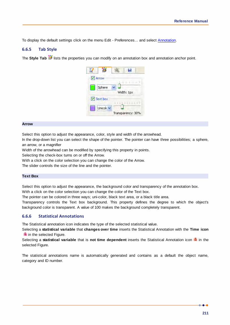
Reference Manual

211

To display the default settings click on the menu Edit - Preferences... and select Annotation.

6.6.5 Tab Style

The Style Tab lists the properties you can modify on an annotation box and annotation anchor point.

Arrow

Select this option to adjust the appearance, color, style and width of the arrowhead.

In the drop-down list you can select the shape of the pointer. The pointer can have three possibilities; a sphere,

an arrow, or a magnifier

Width of the arrowhead can be modified by specifying this property in points.

Selecting the check-box turns on or off the Arrow.

With a click on the color selection you can change the color of the Arrow.

The slider controls the size of the line and the pointer.

Text Box

Select this option to adjust the appearance, the background color and transparency of the annotation box.

With a click on the color selection you can change the color of the Text box.

The pointer can be colored in three ways; uni-color, black text area, or a black title area.

Transparency controls the Text box background. This property defines the degree to which the object's

background color is transparent. A value of 100 makes the background completely transparent.

6.6.6 Statistical Annotations

The Statistical annotation icon indicates the type of the selected statistical value.

Selecting a statistical variable that changes over time inserts the Statistical Annotation with the Time icon

in the selected Figure.

Selecting a statistical variable that is not time dependent inserts the Statistical Annotation icon in the

selected Figure.

The statistical annotations name is automatically generated and contains as a default the object name,

category and ID number.

IMARIS

212

The ID number of the selected object appears on the top of the statistical tab.

For all object types that have time dependent statistical parameters, an individual statistical annotation is

created for every single time point.

Statistical annotations presents always statistical parameter value for the current time point, both in the viewing

area and in the Figure Tree.

Selecting or deselecting the box next to the annotation name in the Figure tree controls the visibility of the

annotation in the viewing area for all time points.

Clicking on the statistical annotation name, the annotation is highlighted and the list of statistical values

appears in the Annotation window.

This list can be customized, by clicking on the Preferences icon .

The option allows you to choose a set of statistical values to be displayed in the viewing area, which differs from

the ones selected from the Statistical table.

By default, statistical annotations are presented in the viewing area without a text box. To create the

annotation box for the statistical annotations select the annotation in the Figure Tree, and then activate the

Text box option under the Style tab . The text box appears in the viewing area and creates the editable

annotation. Select the Text tab and in the description windows write additional details.

Preference

The list of statistical values used in the annotation table, the list can be customized.

Clicking on the icon preferences opens a new window with the list of all possible statistical values available for

the selected object type.

Customization of the list of statistical values is possible by selecting the checkbox next to the statistical value

name. If the box is checked then the statistical value is visible in the annotation table and if is unchecked then

the value is hidden.

This section does not attempt to describe all features of the Statistical values’ calculation in Imaris.

For further information please read the description in the Section Statistics.

Reference Manual

213

6.6.7 Tab Export

Check the check-box if you want to export all figures.

Highlight the figure in the Figure Tree that you want to Export.

With a click on the button Export to HTML you open the Export Figure as HTML window.

Choose the desired file path, enter a file name to save the document.

A web page is created that contains the image name and location, each channel name, the number of time

points, the image size, the number of slices, the voxel sizes, a snapshot of the view that is associated with

the figure, and the figure name.

6.7 Add Time Points...Additional time points can be added to the data set.

Select the required image and click Open.

The time points to be added must contain the same number of channels and be of the same format as the

current data set. A warning message is displayed if the formatting does not match.

Append with Small Time Gap

By default, the check box Append with Small Time Gap is activated. This triggers the same behaviour as in

Imaris versions before Imaris 9.0: The original time information of newly added time points is altered by a

translation on the time line to the end of existing time data. Relative time differences in the added data set stay

the same. The offset between last existing time point and first time point of the added data is set to 1 second.

If the check box is not activated, new time points are added without modifications. This could result in big time

gaps on the time line.

If there is an overlap on the time line between existing time points and newly added ones, the same translation

is applied as described above.

6.8 Delete Time Points...Any time points that are not needed can be deleted.

Parameters

Delete From, To

Specify the time points to be deleted and click OK. The selected time points are automatically deleted from the

data set.

6.9 Add Channels...Adding channels is used to extend or complete the data set information if a microscope can only export one

channel as a file at one time. All channels of a selected data set are added. The size of the data sets must be

identical.

IMARIS

214

Window: Add Channels

Select the required file and click Open.

All channels from this data set are added automatically. If the size of the data set does not match a warning

message is displayed.

6.10 Delete Channels...Deleting channels is used to erase unwanted information in a data set.

Select Channels to Delete

Channel 1...n

Select the channel to be deleted in the Delete Channels box and click OK. The effect is immediately visible on

the image.

See also:Imaris Menu - Open - Reader Configuration

6.11 Remove ImagesUse Remove images to remove images from the current set of open images.

To remove images from a multi-image scene:

1. Check the checkbox beside the required images

2. Click OK to remove the image(s) or Cancel to cancel.

For more about multi-image functionality refer to Add Image... (multi-image)

6.12 Add Slices...Adding slices may become necessary, if through manipulation, or during file export or formatting the data set

consists of less than the originally acquired number of slices.

Window: Add Slices

Select the requested file and click Open.

All slices from this data set are added automatically. The x-, and y-values of the two data sets must be

identical and the same number of channels is required.

6.13 Delete Slice...Parameters

Slice number [1...n]

Specify the slice to be deleted and click OK. The slice is automatically deleted from the data set.

Reference Manual

215

6.14 Crop Time...The total number of time points can be reduced at the beginning or end of the series of images.

Parameters

From, To

Enter the time points to be included in the data set and click OK. All other time points are deleted from the

data set.


6.15 Resample Time...The total number of time points can be reduced to display the images at a faster speed.

Parameters

New Number of Time Points

Specify the number of time points needed and click OK.

The process of resampling the time points takes a while. When the process is finished, the time bar displays

the new number of time points.


6.16 Crop 3D...Cropping the data set allows you to crop the images down to the region of interest. Cropping reduces the size

of the data set and makes it easier and faster to handle the viewing and storing of the images.

Preview

Displays a sectional view of the actual image (current time point). A rectangle, representing the region of

interest (ROI), is overlaid on all three views.

Select Crop Dimensions

X, Y, Z, From, To, Size

To modify the size and the position of the region of interest you can either enter the ranges of x, y, and zcoordinates into the corresponding fields or adjust the region of interest box using the handles directly in theviewer window.

To move the ROI, click inside the rectangle, hold the mouse button down & drag the entire ROI around.

To shape the ROI, click on a handle, hold the mouse button it down and reshape the ROI. Side handles affect

one direction, corner handles two directions.

IMARIS

216

The modifications apply to all slices and all time points of the image.

The displayed values correspond to the changeable voxel value.

Click OK when finished. The data set is cut down to the marked ROI. The rest is erased.


6.17 Resample 3D...Resampling reduces the voxel density in a data set to increase the processing speed. Reducing the data size

also reduce the resolution. Resampling reduces the number of voxels in a grid but keeps the original

relationship between the voxels.

New Size

X, Y, Z

The fields display the current x-, y-, and z-values. The requested values can be directly entered in the fields.

Aspect Ratio

Fixed Ratio X/Y

Fixed Ratio X/Y/Z

The Aspect Ratio of the data set’s dimensions can be kept by checking the respective Fixed Ratio options.

Clicking the OK button resamples the data set to the entered values.

Use a Gaussian filter as low-pass before sampling down an image.

See also:Imaris Menu - Open - Reader ConfigurationMenu Image Processing - Smoothing - Gaussian Filter

6.18 Change Data Type...Type

From

Displays the current data set type.

To

Drop-down list to select the requested data set type from the supported types:

unsigned 8 bit for the range 0...255.

unsigned 16 bit (0...65535).

32 bit float.

Range Adjustment

Check field to determine how the data values are translated during the change.

None

Data values are imported in the new type.

Reference Manual

217

Source Range to Target Range

Maximum data values are scaled to the new range (e.g., 0...255 to 0...65535).

Data Range to Target Range

Actual data range values are interpolated to the new range (e.g., 0...150 to 0...65535).

6.19 File Type Associations...The file association dialog for the thumbnail creator (window Imaris Icon and Thumbnail Settings) is displayed.

File Extensions

Thumbnails will be created and MetaData will be extracted from all checked file types.

Please note: The feature of the thumbnailextractor is not available for the Macintosh users.

.ims

Imaris Series, Imaris Classic

.imx

Imaris Scene

.ics .ids

Nikon ICS

.lsm

Zeiss LSM510

.zvi

Zeiss Axiovision

.lei

Leica LCS

.lif

Leica LIF

.pic

Biorad MRC 1024/600

.rbinf

TILLvisION

.stk

MetaMorph STK

.r3d .dv

Delta Vision

IMARIS

218

.oib .oif

Olympus OIB/OIF

.ipl

Scanalytics IPLab

.ome

Open Microscopy Environment XML

.inf .info

Leica Series

.tif .tiff

Zeiss LSM 410, Zeiss LSM 310, Leica TCS-NT, Leica Series, Leica LCS, Olympus FluoView, Olympus cellR,

PerkinElmer, TIFF series

More

Separated by spaces: e.g. ".ims .ics .lsm .zvi".

2D/3D Indicator

The generated thumbnails are created with or without a 2D/3D indicator.

Show

Check this box to show the indicator at the left upper corner of the thumbnail. There are four different icons to

indicate the image type:

2D Image (colored square).

2D Time Image (pink square and bars).

3D Image (green cube).

3D Time Image (blue cube and bars).

Reference Manual

219

Section 7 View

Please refer to Section:

Slice Ctrl + 1 Slice

Section Ctrl + 2 Section

Gallery Ctrl + 3 Gallery

Easy 3D Ctrl + 4 Easy 3D

3D View Ctrl + 5 3D View

Coloc Ctrl + 7 Coloc

Animation Ctrl + 6 Animation

Fit Ctrl + B

Reset Ctrl + A

Full Screen F11

Navi Ctrl + N

Load Window State

Save Window State

Origin Bottom Left

Origin Top Left

Origin Bottom Right

Origin Top Right

Status Bar Toolbars - Status Bar

Refresh Ctrl + F

Event log

See also:


7.1 SliceHow to Open the Slice?

1. Click on the icon in the Main toolbar. If the Slice icon is not displayed click on the arrow in the group:

Section, Gallery, Easy 3D, and select Slice.

2. Select View - Slice.

3. Press the key combination Ctrl + 1.

See also:

Slice -Mouse & Keyboard Mac

7.1.1 Overview

The Slice mode is the view in which an image is displayed when loading a data set into Imaris. The Slice

representation shows a 2D view from the top in the z-axis. It shows all images in the data set along the z-axis,

so you can inspect any slice along the z-axis for a general overview of the data set.

IMARIS

220

When moving the cursor over the image, the current voxel intensity and the 3D position in the data set (in

brackets) is displayed in the lower left corner of the view.

Additional Information in the Status Bar

The Slice also displays additional information about any given point in the data set. Click a location in the

image display. On the left hand side of the Status Bar the information is displayed as follows:

Ch 1 ... n at (X, Y, Z)

The display shows the voxel intensity values for the channel(s) and the relative 3D position in the data set (in

brackets).

See also:


7.1.2 Slice Toolbar

Slider

To inspect any slice in the data set along the z-axis you use the Slider. Use the slider as follows:

Drag the slider handle in the left control bar up and down.

Select the slider handle with a left mouse click and then use the Arrow-keys up/down on the keyboard.

Select the slider handle with a left mouse click and then press the Home-key or the End-key to display the

first and last slice respectively.

Select the slider handle with a left mouse click and then press the PageDown-key or the PageUp-key to

scroll through the first and last slice respectively in steps.

Enter the desired slice number in the number field at the bottom of the slider.

Button >

Click on the Play/Pause button to see a continuous display through all the slices in the stack. To pause re-

click on the button.

Reference Manual

221

Slice Number Field

The respective slice number is displayed on the bottom of the slider in the number field.

7.1.3 Measure Toolbar

Type

Line

Set the two Measurement Points with two consecutive clicks. The result is displayed in the status field

Distance.

Polygon

All Measurement Points are consecutively connected by lines and the displayed distance is the sum of the

distances between the points.

Grid

Check this box to display a grid in the image.

Distance

The result of the measurement is displayed in the status field distance.

Button Delete

Click on Delete to clear the status field and start a new measurement.


Mouse & Keyboard Functions in the Slice

Ctrl + 1 Activates the Slice

Left-click Set a measurement point


Move down: zoom in


Move down: zoom in


See also:



Mouse & Keyboard Functions in the Slice

Command + 1 Activates the Slice

Click Set a measurement point


IMARIS

222

Shift + Ctrl + click & drag Move up: zoom out

Move down: zoom in

Ctrl + click & drag Pan image









Move down: zoom in


See also:


7.2 SectionHow to Open the Section?

1. Click on the icon in the Main toolbar. If the icon Section is not displayed click on the arrow in the group:

Slice, Gallery, Easy 3D, and select Section.

2. Select View - Section.


7.2.1 Overview

The Section lets you inspect the environment of any given point within the data set by showing the cut through

the point in the x-, y-, and z-axes or a defined portion of the data set (several slices together).

The illustration below shows the coordinates in the three different display areas of the section.

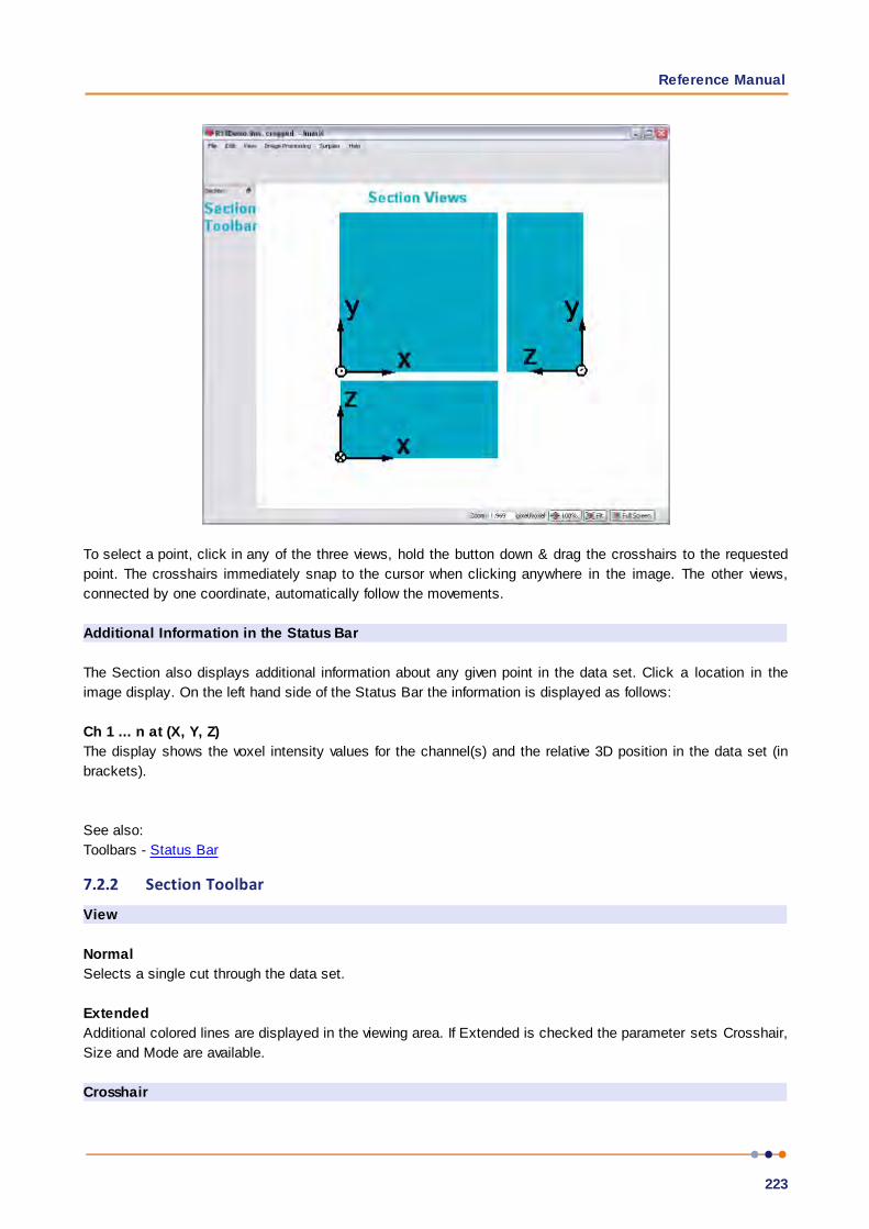
Reference Manual

223

To select a point, click in any of the three views, hold the button down & drag the crosshairs to the requested

point. The crosshairs immediately snap to the cursor when clicking anywhere in the image. The other views,

connected by one coordinate, automatically follow the movements.


The Section also displays additional information about any given point in the data set. Click a location in the

image display. On the left hand side of the Status Bar the information is displayed as follows:

Ch 1 ... n at (X, Y, Z)

The display shows the voxel intensity values for the channel(s) and the relative 3D position in the data set (in

brackets).

See also:


7.2.2 Section Toolbar

View

Normal

Selects a single cut through the data set.

Extended

Additional colored lines are displayed in the viewing area. If Extended is checked the parameter sets Crosshair,

Size and Mode are available.

Crosshair

IMARIS

224

The parameter set Crosshair is only available, if Extended is checked in the parameter set View (see above).

Normal

You may eliminate the Crosshair display on the image by unchecking the box. It is then only visible at the

edges.

Extended

Select a portion of the data set in the x-, y-, and z-direction to be displayed. In the main screen, separate the

two crosshairs. The planes between the crosshairs are rendered in the views showing the other axis. This

allows you to see only certain interior structures without both the top and the bottom.

The image shows the white crosshair line together with colored focus range lines.

The focus range can be set in any of the three directions as follows: Move the cursor on a colored line. The

cursor changes its form to a straight arrow with a bar.

Drag the line in the respective direction. The range is extended or reduced. Its depth is reflected in the x-, y-,

and z-fields in the Size display. The Size values are indicated in the data set’s dimensions, e.g., in m. It

can also be adjusted directly by entering values in the Size fields (see below) or by means of their up and

down arrows.

Uncheck the Crosshair – Normal and/or Crosshair – Extended boxes to eliminate the crosshair and/or the focus

range lines display on the image.

Size fields

The parameter set Size is only available, if Extended is checked in the parameter set View (see above). Display

of the actual x-, y-, and z-position of the extended Crosshair. The positions can also be adjusted directly by

entering values in the fields or by means of their up and down arrows.

Mode

The parameter set Mode is only available, if Extended is checked in the parameter set View (see above). Here

you may choose the best display mode for the slice portion.

MIP

Calculated maximum over all slices in the range.

Mean

Calculated mean value over all slices in the range.

Blend

Calculated upon the transparency of the slices.


Mouse & Keyboard Functions in the Section

Ctrl + 2 Activates the Section

Left-click Set the section center


Move down: zoom in

Reference Manual

225


Move down: zoom in


See also:



Mouse & Keyboard Functions in the Section

Command + 2 Activates the Section

Click Set the section center



Move down: zoom in










Move down: zoom in


See also:


7.3 GalleryHow to Open the Gallery ?

Click on the icon in the Main toolbar. If the Gallery icon is not displayed click on the arrow in the group:

Section, Slice, Easy 3D, and select Gallery.

Select View - Gallery.


See also:

Gallery - Mouse & Keyboard Mac

IMARIS

226

7.3.1 Overview

The Gallery displays all available slice images of the data set. In the Gallery you can adapt the display to your

needs to gain more information from the slice series. When the Gallery is selected, all slices are displayed.

Click on images to select or deselect them. Selected images are marked with a colored frame. Holding the

Shift-key lets you select a continuous series of images. Hold the Ctrl-key to select various images spread over

the gallery.


The status bar indicates which of how many available pages is currently being displayed, and how many slices

have been selected. Changes in the Gallery only affect the current display and do not crop the data set.

See also:Toolbars - Status Bar

7.3.2 Gallery Toolbar

In the Gallery the following display and selection controls are available:

Slice

By clicking on the arrows, you move up and down the images in the gallery one by one. This is especially

useful whenever the display on the screen does not include all the slices.

Page

If there are more images than displayed on screen, move up and down the pages by clicking on the arrows or

go directly to the first or last page by using the respective buttons.

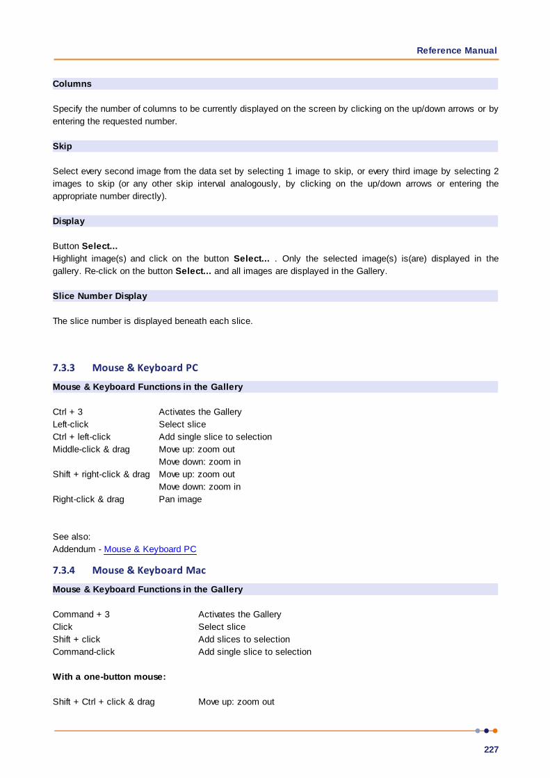
Reference Manual

227

Columns

Specify the number of columns to be currently displayed on the screen by clicking on the up/down arrows or by

entering the requested number.

Skip

Select every second image from the data set by selecting 1 image to skip, or every third image by selecting 2

images to skip (or any other skip interval analogously, by clicking on the up/down arrows or entering the

appropriate number directly).

Display

Button Select...

Highlight image(s) and click on the button Select... . Only the selected image(s) is(are) displayed in the

gallery. Re-click on the button Select... and all images are displayed in the Gallery.

Slice Number Display

The slice number is displayed beneath each slice.


Mouse & Keyboard Functions in the Gallery

Ctrl + 3 Activates the Gallery

Left-click Select slice

Ctrl + left-click Add single slice to selection


Move down: zoom in


Move down: zoom in


See also:



Mouse & Keyboard Functions in the Gallery

Command + 3 Activates the Gallery

Click Select slice

Shift + click Add slices to selection

Command-click Add single slice to selection



IMARIS

228

Move down: zoom in










Move down: zoom in


See also:


7.4 Easy 3DHow to Open the Easy 3D?

Click on the icon in the Main toolbar. If the icon Easy 3D is not displayed click on the arrow in the group:

Section, Gallery, Slice, and select Easy 3D.

Select View - Easy 3D.


See also:

Easy 3D - Mouse & Keyboard Mac

7.4.1 Overview

The Easy 3D provides a quick fixed view with a few parameters for rendering and light setting. This lets you

explore the data set in the 3D mode before doing any further processing.

Reference Manual

229

7.4.2 Easy 3D Toolbar

Rendering

MIP

(Maximum Intensity Projection) - Shows the maximum intensity of all layers along the viewing direction.

Blend

Shows the color obtained by blending all values along the viewing direction and including their transparency. If

Blend is selected, the parameter set Light is available (see below).

Light

If Blend is selected (see above), the parameter set Light is available.

Light

Check the box to switch the light on and adjust the following parameters. There are two predefined light setting

parameters in Easy 3D Blend to choose from.

Left

Light from the left, shadow to the right.

Right

Light from the right, shadow to the left.

Button Settings...

In Blend mode, with light enabled, click the button Settings.... The Easy 3D Settings dialog box displays (see

below).

Calculate

IMARIS

230

Auto

The image is calculated and displayed automatically.

Manual

The image calculation starts after you click on the button Calculate. If you select Manual as calculation mode,

the button Calculate is available.

Button Calculate

Click on this button to start the calculation for the Easy 3D image view. The button is only available, if you

select Manual as calculation mode.

Window: Easy 3D Settings

Light

Directional Intensity

Controls the brightness of structures that are illuminated from the light source.

Ambient Intensity

Controls the brightness of structures that are in the shadow. The default (0) means that structures completely

in the shadow are black. The higher the value the brighter the picture and the lower the shadowing contrasts.

Channel Opacity Combination

Allows you to control the opacity of the image.

Opaque

Translucent

Custom

Select Opaque, Transparent, or Custom opacity. It affects only the behavior of interleaving structures of two or

more channels.


Mouse & Keyboard Functions in the Easy 3D View

Ctrl + 4 Activates the Easy 3D


Move down: zoom in


Move down: zoom in


See also:


Reference Manual

231


Mouse & Keyboard Functions in the Easy 3D View

Command + 4 Activates the Easy 3D



Move down: zoom in










Move down: zoom in


See also:


7.5 ColocIn fluorescent microscopy, colocalization describes the presence of two fluorochromes at the same physical

location. ImarisColoc provides extended functionality for the analysis and visualization of colocalization in multi-

channel data sets. It provides an automated selection of colocalization based on a method introduced by

Costes & Lockett at the NIH, NCI/SAIC.

Coloc processes 2D, 3D, and 4D data sets. It operates on two channels simultaneously and measures the

degree of overlap of the two channels.

With Coloc you can determine and display locations within the data set with common information from all

channels, e.g., to illustrate where all types of proteins can be found simultaneously or to detect low-density

tissues in all channels.

The desired range for signal analysis can be limited by defining intensity thresholds or sets of intensity values

for each of the involved channels. All voxels falling inside everyone of these channel-specific intensity limits

represent a colocalization. They are emphasized in the view and statistics are calculated and displayed. When

the selection is changed, the numeric and visual feedback happens in real-time.

The result of the colocalization as a whole can be saved as a separate channel, which can then be processed

and viewed as any originally acquired channel in Imaris. Multiple colocalization images are easily combined into

a single view in Imaris Surpass.

IMARIS

232

Coloc is an optional module within the Imaris program and is not available as a standalone program.

How to Display the Coloc Main Screen?

Click on the Coloc icon in the Main toolbar,

Select View - Coloc,


See also:

Coloc - Mouse & Keyboard Mac

7.5.1 Overview

The Coloc main screen consists of different areas:

Channel Histogram (channel A, channel B). This area allows the selection of the two channels for the

colocalization analysis.

Preview Window. This area visualizes the data set together with a preview of the colocalized region.

2D Histogram. This area displays a two-dimensional intensity histogram of the selected channels. It reflects

the distribution of pairs of voxel intensities occurring in the two selected channels. The range of intensity

pairs considered as colocalized can be defined on the histogram.

Volume Statistics. This area displays statistics about the resulting colocalized volume. The display adapts

instantly to all modifications in the selection.

ROI Definition. This feature allows you to define a region of interest (ROI) for the entire analysis.

Coloc Toolbar. The Coloc toolbar contains several sections with all possible selection and definition tools and

settings for the histograms, the thresholding, and the display as well as the buttons for the color definition

and the build of the Coloc channel.

Reference Manual

233

7.5.2 Channel Histogram

This area allows the selection of the two channels for the colocalization analysis. The intensity histograms are

displayed for the currently selected channels.

Select Channel A and Channel B

The two channels for colocalization detection must be selected first.

Select channel A and channel B from the drop-down lists. The 1D and 2D intensity histogram displays are

updated.

Adjust Threshold

The threshold for each channel can then be defined by clicking in the histogram, dragging the colored line

directly, or by entering the value in the threshold field.

Adjust Histogram Settings

If necessary, you can adjust in the Coloc toolbar the histogram mode and histogram options.

See also:

Coloc - Coloc Toolbar

Coloc - Mouse & Keyboard PCColoc - Mouse & Keyboard Mac

7.5.3 Preview Window

This area visualizes the data set together with a preview of the colocalized region. It displays a Slice

representation of the data set, i.e. a 2D view from the top in the z-axis direction. On the left hand side, a sliding

bar with a handle allows inspecting and displaying the single slices in the data set along the z-axis. The

Preview window updates in real-time the display of the colocalized region based on the actual settings of the

colocalization parameters. The original channels can be switched on or off in the Display Adjustments window.

Time Settings

There are no time-dependent parameters for the colocalization analysis. The Preview window always displays

the currently selected time point of the data set. The values in the Statistics window always refer to the volume

of the current time point. However, when the Build Coloc Channel button is pressed, the Coloc channel and

statistical values for all time points are calculated.

See also:

Menu Edit - Show Display Adjustment


7.5.4 2D Histogram

This area displays a two-dimensional intensity histogram of the selected channels. It reflects the distribution of

pairs of voxel intensities occurring in the two selected channels. The range of intensity pairs considered as

colocalized can be defined on the histogram.

Adjust Channel Thresholds

IMARIS

234

Effects of the modification are instantly visible in the channel histogram A and B, and in the Preview window.

Selection Mode Threshold

The channel thresholds are visible in form of a rectangle.

Point with the cursor on the 2D histogram.

Click on the histogram to determine the thresholds. The edge of the overlaid hatched area (indicating the

selected voxel intensity range for colocalization) jumps on the marked spot.

Click on the edge and drag it to any another position in the histogram.

Selection Mode Polygon

The channel thresholds are visible as an intensity area in form of a free configurable polygon.

You draw the polygon on the 2D histogram. This method is especially useful for eliminating channel bleed

through regions along the border of the lower intensity bins. After checking the Polygon mode, the overlaid

threshold rectangle in the 2D histogram is converted into a polygon with four corner points. You can now start

to modify this polygon or to draw a completely new one. The initial point of the polygon is visible as white filled.

Set Point

Press and hold the Shift-key. The cursor turns into a cross with a little sign. Click on the 2D histogram with the

left mouse button to place a point (vertex). Any additional point connects with lines to the initial point and the

last point inserted.

Insert Point in a Line

Press and hold the Shift-key. The cursor turns into a cross with a little '' + '' sign. Point on the line between the

two vertices and click on the line with the left mouse button to add a point.

Automatic Point Setting

Press and hold the Ctrl-key. The cursor turns into a cross with a little '' + '' sign and a stack symbol. Drag the

cursor around. New vertices are added automatically at each change of cursor position.

Move Point

Point on one of the vertices, click & drag the vertex around to the desired location. The polygon changes its

shape.

Move Line

Point on a line between two vertices, click & drag the line around to the desired location. The polygon changes

its shape.

Move Polygon

Point somewhere beside of the polygon edge, click & drag the polygon around to the desired location.

Delete Point

Shift + click on a point to delete the point.

See also:

Coloc - Coloc Toolbar (selection Mode Threshold or Polygon)

Reference Manual

235

7.5.5 Volume Statistics

The values are updated in real-time and refer to the entire volume data of the current time point, regardless of

the settings for the histogram mode. The values are calculated by the following formulas.

Please note: The calculated Coloc Volume Statistics are not automatically saved in the data set. To

save or export the statistics you have to build a coloc channel (Coloc - Coloc Toolbar - Build Coloc

Channel). For publishing Coloc statistical values please use only the statistics reported in the

Channel Properties.

Due to a real-time response, some of the statistical values shown in the main Coloc window are generated from

a sub-sampled data set. The accuracy of these values depends on the variability introduced by the sub-

sampling procedure.

Depending on the data set, the difference between the values reported in the Channel Properties (a high

accuracy values, produced from the entire data set) and these values (calculated from sub-sampled data set)

may differ significantly.

Definitions

Regions:

Data set All data set voxels

Coloc Colocalized voxels

Object A Voxels with channel A intensity above threshold A

Object B Voxels with channel B intensity above threshold B

ROI Region of interest

Indicators:

N Number of voxels

SAi Channel A intensity of voxel

SBi Channel B intensity of voxel

SAavg,

Coloc

Average channel A intensity in the Coloc region

Volume A Number of voxel channel A x voxel volume

Volume B Number of voxel channel B x voxel volume

Material A Channel A voxel signal intensity

Material B Channel B voxel signal intensity

Number of colocalized voxels

Total count of colocalized voxels Ncoloc .

Please note:

Ncoloc is the number of colocalized voxels for the defined region of interest (ROI).

Colocalization statistics are all calculated using the ROI.

% of data set colocalized

Percentage of total data set voxels colocalized.

IMARIS

236

% of volume A above threshold colocalized

Percentage of channel A voxels above threshold A colocalized.

% of volume B above threshold colocalized

Percentage of channel B voxels above threshold B colocalized.

% of material A above threshold colocalized

Percentage of channel A material above threshold A that is colocalized.

% of material B above threshold colocalized

Percentage of channel B material above threshold B that is colocalized.

% of ROI colocalized

Percentage colocalization of channel A and channel B volume inside the region of interest.

% of ROI material A colocalized

Percentage colocalization of ROI channel A material.

Reference Manual

237

% of ROI material B colocalized

Percentage colocalization of ROI channel B material.

Pearson`s coefficient in colocalized volume

Pearson correlation of channel A and channel B inside the colocalized region.

Please note: The correlation value ranges between 1 and -1. A value of 1 represents perfect

correlation, 0 no correlation, and -1 perfect inverse correlation.

Pearson`s coefficient in data set volume

Pearson correlation of channel A and channel B inside the entire data set volume.

Pearson`s coefficient in ROI volume

Pearson correlation of channel A and channel B inside the region of interest.

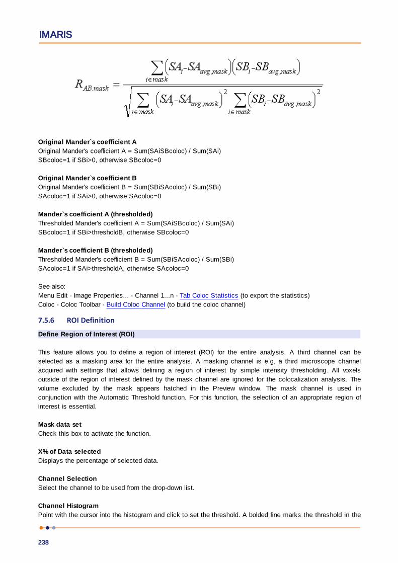
IMARIS

238

Original Mander`s coefficient A

Original Mander's coefficient A = Sum(SAiSBcoloc) / Sum(SAi)

SBcoloc=1 if SBi>0, otherwise SBcoloc=0

Original Mander`s coefficient B

Original Mander's coefficient B = Sum(SBiSAcoloc) / Sum(SBi)

SAcoloc=1 if SAi>0, otherwise SAcoloc=0

Mander`s coefficient A (thresholded)

Thresholded Mander's coefficient A = Sum(SAiSBcoloc) / Sum(SAi)

SBcoloc=1 if SBi>thresholdB, otherwise SBcoloc=0

Mander`s coefficient B (thresholded)

Thresholded Mander's coefficient B = Sum(SBiSAcoloc) / Sum(SBi)

SAcoloc=1 if SAi>thresholdA, otherwise SAcoloc=0

See also:

Menu Edit - Image Properties... - Channel 1...n - Tab Coloc Statistics (to export the statistics)

Coloc - Coloc Toolbar - Build Coloc Channel (to build the coloc channel)

7.5.6 ROI Definition

Define Region of Interest (ROI)

This feature allows you to define a region of interest (ROI) for the entire analysis. A third channel can be

selected as a masking area for the entire analysis. A masking channel is e.g. a third microscope channel

acquired with settings that allows defining a region of interest by simple intensity thresholding. All voxels

outside of the region of interest defined by the mask channel are ignored for the colocalization analysis. The

volume excluded by the mask appears hatched in the Preview window. The mask channel is used in

conjunction with the Automatic Threshold function. For this function, the selection of an appropriate region of

interest is essential.

Mask data set

Check this box to activate the function.

X% of Data selected

Displays the percentage of selected data.

Channel Selection

Select the channel to be used from the drop-down list.

Channel Histogram

Point with the cursor into the histogram and click to set the threshold. A bolded line marks the threshold in the

Reference Manual

239

histogram and the corresponding value is indicated in the threshold field. The masked volume of the data set

appears hatched in the Preview window. Drag the cursor in the histogram to modify the threshold. Effects of the

modification are instantly visible in the threshold field as well as in the Preview window.

Threshold Value

Editable threshold value field.

Mask Channel and Automatic Threshold

When the mask is set as required, click the button Automatic Thresholding to calculate the thresholds. Build

the colocalization channel by clicking the button Build Coloc Channel.

See also:

Coloc - Coloc Toolbar - Automatic Thresholding

Coloc - Coloc Toolbar - Build Coloc Channel


7.5.7 Coloc Toolbar

The Coloc toolbar contains several sections with all possible selection and definition tools and settings for the

histograms, the thresholding, and the display as well as the buttons for the color definition and the build of the

Coloc channel.

Selection Mode

You can define, for each of the channels separately, an intensity value as a threshold. Only voxels with an

intensity value above the specified threshold will be considered for the colocalization analysis. The two

thresholds are visible and can be set in four different ways:

1. As a hatched region with a bold line on the channel histograms.

2. As a value in the Threshold field of each channel (channel histogram).

3. As a hatched region with bold lines on the 2D histogram. The region always contains the top right part of the

histogram. The left and lower bold lines define the intensity thresholds for the two channels.

4. As an active contour in the Preview window.

Threshold

To adjust the threshold value using the mouse (see above 1. and 3.), select this mode.

Polygon

To draw a polygon line in the 2D histogram (see above 4.) select this selection mode.

Automatic Thresholding

Please refer to Section Coloc - Coloc Toolbar - Automatic Thresholding.

Histogram Mode

The histogram mode options define the voxels selection for the colocalization calculation within the data set.

Single Slice

The 2D histogram is calculated and displayed for the current slice only.

IMARIS

240

Single Time Point

The 2D histogram is calculated and shown for the entire 3D stack of the current time point. This mode allows

for faster browsing through the data set along the z-axis.

All Time Points

The 2D histogram is calculated and shown for an entire time data set, i.e. for all time points within the 4D data

set.

Histogram Options

The histogram mode options are used to define the display of the 1D and 2D histograms.

Ignore Border Bins

A border bin is always the first and last value in a histogram. Often a lot of voxels fall into the bin with the

lowest intensity. In a frequency plot this causes a massive and unnecessary downscale of all other intensity

bins which are of more interest. The border bins can therefore be ignored when scaling the display of the

histogram. Ignore is selected as default. With most data sets, checking the Ignore Border Bin and Logarithmic

options allows a more representative histogram display.

Logarithmic

The frequency plot is shown in a logarithmic scaling instead of a linear scaling.

Color Coded

Applies a false color look-up table to the histogram to improve the visibility of intensity differences. The high

frequencies (bins in the 2D histogram into which a lot of voxels accumulate) are shown in yellow-to-white, bins

with little voxels are shown in blue-to-black.

Coloc Intensities

The Coloc intensities option defines the brightness of the calculated colocalization displayed in the Preview

window.

Source Channels

Uses the intensities of the two channels for displaying the intensity of a colocalized voxel as the square root of

the product of the intensities of the original channels.

Constant Value

Displays the intensity of a colocalized voxel defined by the specified value. No distinction is made whether high-

intensity or low-intensity voxels colocalize as long as they are within the selection.

Coloc Color

Coloc color allows you to specify personal color settings for the colocalization display in the Preview window.

Button Edit

Clicking on the button Edit opens the Color window. You can either select one of the predefined colors to apply

on the colocalization areas or define, add, and apply your own color definitions.

Button Build Coloc Channel

Please refer to Section Coloc - Coloc Toolbar - Build Coloc Channel.

Reference Manual

241

Button Build Time Dep. Coloc

Please refer to Section Coloc - Coloc Toolbar - Build Coloc Channel.

Button Channel Statistics

Please refer to Section Menu Edit - Image Properties... - Channel 1...n - Tab Coloc Statistics.

See also:

Coloc - Channel Histogram

Coloc - Preview Window

Coloc - 2D Histogram

7.5.7.1 Automatic ThresholdingButton Calculate Thresholds

This button performs an automatic threshold run on both channels based on an algorithm developed by Costes

and Lockett at the National Institute of Health, NCI/SAIC, which is based on the exclusion of intensity pairs that

exhibit no correlation (Pearson’s correlation below zero).

The automatic threshold search is done using the 2D histogram. Starting with the highest intensity value, the

algorithm reduces the threshold value step by step along a line (see figure below) and computes the correlation

coefficient of the image using only voxels with intensities below the threshold. The algorithm continues reducing

the thresholds until the correlation reaches 0, thus defining the automatic threshold.

P-Value

PSF Width

As the size of the Point Spread Function please enter the length along the Z Axis. This can be a calculated

theoretical length.

You can find links to calculators on the web e.g. on the Bitplane homepage.

The default in Imaris is not actually related to the PSF but only to the diagonal of the voxel size.

IMARIS

242

For more information about the P-Value and PSF Width please refer to the following publication:

Automatic and Quantitative Measurement of Protein-Protein Colocalization in Live Cells

Sylvain V. Costes,*y Dirk Daelemans,z Edward H. Cho,* Zachary Dobbin,* George Pavlakis,z

and Stephen Lockett*

* Image Analysis Laboratory, National Cancer Institute, Frederick, Maryland;

y National Cancer Institute/Science Applications International Corporation, Frederick, Maryland; and

z Human Retrovirus Section, National Cancer Institute, Frederick, Maryland

Biophysical Journal Volume 86 June 2004 3993-4003

7.5.7.2 Build Coloc ChannelButton Build Coloc Channel

Clicking this button calculates the colocalization channel according to the selected settings and adds it to the

data set. The channel can then be saved and is part of the data set.

Button Build Time Dep. Coloc

Clicking this button calculates the colocalization channel according to the selected settings (calculating an

automatic threshold individually for each time point) and adds it to the data set. The channel can then be saved

and is part of the data set.

Save Coloc Channel

Before the channel is added permanently to the data set it must be saved. In the menu bar select File – Export

or click the Export button in the toolbar. The Export box is displayed. Select the directory and enter the name

for the file to be saved or confirm the suggestion. Select the requested file format and click OK. The data set is

saved.

Button Channel Statistics (for the new Coloc channel)

After building the Coloc channel, its statistics become available in the Image Properties. The button Channel

Statistics displays directly the Image Properties window with the statistics for the calculated channel. The

name of the channel, the description of the source channels and the selection method are indicated and

displayed in the Image Properties on the Tab Coloc Statistics.

Export Statistics

The statistics can be exported.

Button Export

In the Image Properties window click the Export button. The Export Coloc Statistics window is displayed.

Select the directory and enter the name for the file to be saved. The statistics are saved as .csv Excel file and

can be opened directly with Microsoft Excel.

See also:


Reference Manual

243

7.5.8 Basic Operation

The basic use of Coloc in the daily work flow comprises the following steps:

Select the channels.

Adjust selection mode and histogram mode.

Set thresholds.

Check the statistics.

Build and save the Coloc channel.

Select Channel A and Channel B

In the 1D histograms select channel A and channel B from the drop-down lists. The 1D and 2D intensity

histogram displays are updated.

Adjust Selection Mode and Histogram Mode

Before you set the thresholds, please check the appropriate parameters in the Coloc toolbar on the right hand

side of the screen:

Check as Selection Mode Threshold.

Decide, which Histogram Mode you need. Choose Single Slice for calculating the histogram for the current

slice only. Or choose Single Time Point to calculate the histogram for the entire 3D time point. Or choose All

Time Points for the entire 4D image.

Set Thresholds

Colocalization occurs where the voxels are above threshold in channel A and channel B. You can define, for

each of the channels separately, an intensity value as a threshold. Only voxels with an intensity value above the

specified threshold will be considered for the colocalization analysis. The two thresholds are visible and can be

set in four different ways:

1. As a hatched region with a bold line on the channel histograms.

2. As a value in the Threshold field of each channel (channel histogram).

3. As a hatched region with bold lines on the 2D histogram. The region always contains the top right part of the

histogram. The left and lower bold lines define the intensity thresholds for the two channels.

4. As an active contour in the Preview window.

A. On the 1D Channel Histogram

Point with the cursor on the histogram. The cursor turns into a cross.

Click on the histogram to determine a threshold. The bold left line of the overlaid hatched area (indicating the


Click on the line and drag it to another position in the histogram. Effects of the modification are instantly

visible in the other indications as well as in the Preview window.

Perform for both channels until the settings are as desired.

B. By Entering a Value

Click in the Threshold field of one of the channels and enter a value, then press Enter. The bold left line of the

overlaid hatched area (indicating the selected voxel intensity range for colocalization) jumps on the marked

IMARIS

244

spot. Effects of the modification are instantly visible in the other indications as well as in the Preview display.

Perform for both channels until the settings are as desired.

C. On the 2D Histogram

Point with the cursor on the 2D histogram. The cursor turns into a cross.

Click on the histogram to determine the thresholds. The edge of the overlaid hatched area (indicating the


Click on the edge and drag it to any another position in the histogram.

D. On the Preview Window

Click with the cursor on the image in the Preview window. An active contour is displayed, outlining image

elements brighter than the location clicked.

Drag the line on the image to define the threshold of channel A. The selection works best when starting with

brighter spots and dragging towards darker areas.

Press and hold the Shift-key, click with the cursor on the image, then drag the line to determine the threshold

of channel B.

Check the Statistics

The statistical values are updated in real-time and refer to the entire volume data of the current time point,

regardless of the settings for the histogram mode. For details please refer to Section Coloc - Volume Statistics.

Build Coloc Channel

Button Build Coloc Channel

Clicking this button calculates the colocalization channel according to the selected settings and adds it to the

data set.

Save Coloc Channel

Before the channel is added permanently to the data set it must be saved. In the menu bar select File - Export

or click the Export button in the toolbar. The Export box is displayed. Select the directory and enter the name

for the file to be saved or confirm the suggestion. Select the requested file format and click OK. The data set is

saved.

7.5.8.1 Advanced ExamplesThe colocalization channel can be visualized like any other channel in Imaris. In the following examples, a

Coloc channel was built on the retina data set.

Visualize the Coloc Channel in Easy 3D

Example 1: Visualize and Adjust the Coloc Channel in Imaris Easy 3D

After building the Coloc channel, click on the Easy 3D button in the Imaris menu bar.

Check the desired Rendering mode parameters and adjust the Settings if necessary, then click the

Calculate button. The 3D image of channel is calculated and displayed.

Reference Manual

245

As the colocalized region always lays inside the initial channels, making the initial channels invisible or more

transparent allows a better view of the colocalized region.

In the Imaris menu bar select Edit – Show Display Adjustment.

In the Display Adjustments window uncheck one of the two original channels, then click the button

Calculate again. The 3D image of the original and the Coloc channel is calculated and displayed.

In the Imaris menu bar select Edit – Show Display Adjustment.

In the Display Adjustment window select the Coloc channel and adjust its settings.

In the Display Adjustment window select the remaining original channel and adjust its settings. In this

example the channel is set as partly opaque.

After each modification, click the Calculate button again to calculate the result.

Visualize the Coloc Channel in Surpass

The colocalization channel can be visualized like any other channel in Surpass.

Example 2: Create Surfaces of the Coloc Channel and Add the Two Initial Channels as Volume Rendering

After building the Coloc channel, click on the Surpass button in the Imaris menu bar.

In the Objects toolbar click the Add New Surfaces button.

In the Surfaces Properties window check and select the Coloc channel.

Select the desired parameters. In this example, we set the threshold just below the lowest intensity values in

the histogram.

In the menu Surpass select Volume.

In the Imaris menu bar select Edit – Show Display Adjustment and uncheck the Coloc channel. The Surpass

Volume object displays only the two initial channels. Then select the two initial channels and adjust their

settings, e.g. decrease the blend opacity.


Coloc Mouse & Keyboard Functions

Ctrl + 7 Activates the Coloc view


When using one of the methods to modify the threshold values, the other indications as well as the Preview

display are updated in real-time.

Histogram Channel A and Histogram Channel B

Left-click on histogram Set new threshold

Left-click on line & drag Move threshold

2D Histogram

Left-click Set channel A and channel B thresholds

Left-click on line & drag Move channel A and channel B thresholds

Preview Window

IMARIS

246

Left-click & drag Set threshold channel A

Shift + left-click & drag Set threshold channel B


Move down: zoom in


Move down: zoom in



2D Histogram

Shift + left-click Add new point (any additional point connects to the last inserted point)

Shift + left-click

on connecting line

Insert point in a line

Shift + left-click

on point

Delete point

Ctrl + left-click Add multiple new points

Left-click & drag

(on point or line)

Move point or line

Left-click & drag

(outside polygon)

Move polygon

Delete Delete single point


Coloc Mouse & Keyboard Functions

Command + 7 Activates the Coloc view


When using one of the methods to modify the threshold values, the other indications as well as the Preview

display are updated in real-time.

Histogram Channel A and Histogram Channel B

Click on histogram Set new threshold

Click on line & drag Move threshold

2D Histogram

Click Set channel A and channel B thresholds

Click on line & drag Move channel A and channel B thresholds

Preview Window

Click & drag Set threshold channel A

Shift + click & drag Set threshold channel B


Reference Manual

247


Move down: zoom in










Move down: zoom in



2D Histogram

Shift + click Add new point (any additional point connects to the last inserted point)

Shift + left-click

on connecting line

Insert point in a line

Shift + left-click

on point

Delete point

Command + click Add multiple new points

Click & drag

(on point or line)

Move point or line

Click & drag

(outside polygon)

Move polygon

Delete Delete single point

7.6 AnimationThe Key Frame Animation function defines several subsequent views (key frames) of your image, which will be

used to create an animation. Imaris generates smooth transitions between the selected views by interpolation.

How to Open the Key Frame Animation Window?

1. Click on the icon in the Main toolbar.

2. Select View - Animation.


See also:

Menu Edit - Preferences... - 3D View

Animation - Mouse & Keyboard Mac

IMARIS

248

7.6.1 Overview

The Key Frame Animation consists of different areas:

At the bottom of the screen the following windows are displayed: the Key Frame Window, the Rotations

Window, the Animation Window, the State selection, and the Strip Window.

7.6.2 Key Frame Window

In the Key Frame window you define and manage the key frames of your movie.

Button Add

Use this button to insert user-defined key frames in the strip sequence.

Button Modify

Use this button to modify user-defined key frames in the strip sequence.

Button Delete

Use this button to delete user-defined key frames in the strip sequence.

Button Delete All

Click on this button to delete all user-defined key frames in the Strip window.

Large spaces between the user-defined key frames (thick blue lines) will cause that section of the

movie to play more slowly. Placing the lines close together will cause that section of the movie to

play more quickly. Use this button to set a constant speed throughout the entire movie.

Button II<

Button II>

With the arrow buttons you step to the previous (arrow to the left) or next (arrow to the right) user-defined key

frame.

Reference Manual

249

Buttons Overview

Add Add new user-defined key frame

Mod. Modify active, user-defined key frame

Del Delete active, user-defined key frame

Del. All Delete all key frames

II< Go to Previous user-defined key frame

II> Go to Next user-defined key frame

For the complex use of these buttons please refer to Section Animation - Strip Window.

See also:

Animation - Create Animation

7.6.3 Rotations Window

Use the templates to quickly define standard camera motions for the key frame animation system.

Templates

Select one of the predefined templates.

You can customize your animation rotation by choosing one of the following options: +360 horizontal, + 180

horizontal, - 360 horizontal, - 180 horizontal, +360 vertical, + 180 vertical, - 360 vertical, - 180 vertical

The key frames are inserted automatically. Click on the button Play to see the animation.

Button Custom

Click on this button to display the Custom Rotation window to freely define the rotation (see below).

Space

Screen

The rotation axis is associated to the x-, y-, and z-axis of the screen.

World

The rotation axis is associated to the x-, y-, and z-axis of the data set.

Axis

X

Y

Z

Turn along the x-, y-, or z-axis.

Direction

+

Turn to the left.

-

Turn to the right.

IMARIS

250

Angle

Select or type in the desired angle.

Button OK

Click on this button to accept the changes.

Button Cancel

Click on this button to cancel the changes.

7.6.4 Animation Window

Frames

The number in the field Frames indicates the number of thin blue lines within the Strip Panel. This number

defines the duration of animations.

Button Settings ...

To open and adjust the Key Frame settings click on this button. For details please refer to Section Menu Edit -

Preferences... - 3D View.

Button >

Click on this button (arrow to the right - Play/Pause) to start the movie preview. To pause the movie preview re-

click on this button.

Button O

To record the movie click on this button (red dot - Record). Selecting this button the Export Movie window is

displayed (see below).

Window: Export Movie Window

File name

Enter a file name.

Export type

Select the desired file type (TIFF series, or AVI).

Movie Settings

Compression Factor

Select a compression factor between 0 (high quality) and 100 (low quality), the default setting is 5. Use the

slider to set the compression factor between 0 and 100. A lower factor results in a lower compression and

therefore a better quality, but also in a larger movie file.

Frame Rate

Define how many frames are displayed per second.

Play Movie with default Media Player when finished

Check the box to play the movie with the default media player when finished.

Menu Edit - Preferences... - Surpass (default Key Frame settings)

Reference Manual

251

7.6.5 Play Back State

In the State selection you can adjust the play back settings.

Camera

Check: Play back the previously recorded Camera positions for each key frame.

Uncheck: Do not play back the recorded Camera positions. The Camera stays in the same position. You can

change the Camera position manually while playing the animation.

Time Points

Check: Play back the previously recorded Time Points for each key frame.

Uncheck: Do not play back the recorded Time Points. The Time Points do not automatically change during

the animation. You can change the Time Points manually while playing the animation.

Colors

Check: Play back the previously recorded Colors for each key frame.

Uncheck: Do not play back the recorded Colors. The Colors do not automatically change during the

animation. You can change the Colors manually while playing the animation.

Display Adjustments

Check: Play back the previously recorded Display Adjustments for each key frame.

Un-check: Do not play back the recorded Display Adjustments. The Display Adjustments do not

automatically change during the animation. You can change the Display Adjustments manually while playing

the animation.

Clipping Plane (Position)

Check: Play back the previously recorded Clipping Plane positions for each key frame.

Uncheck: Do not play back the recorded Clipping Plane positions. The Clipping Plane positions do not

automatically change during the animation. You can change the Clipping Plane positions manually while

playing the animation.

Orthogonal Slicer (Position)

Check: Play back the previously recorded Orthogonal Slicer positions for each key frame.

Uncheck: Do not play back the recorded Orthogonal Slicer positions. The Orthogonal Slicer positions do not

automatically change during the animation. You can change the Orthogonal Slicer positions manually while


Oblique Slicer (Position)

Check: Play back the previously recorded Oblique Slicer positions for each key frame.

Uncheck: Do not play back the recorded Oblique Slicer positions. The Oblique Slicer positions do not

automatically change during the animation. You can change the Oblique Slicer positions manually while


Objects Show/Hide (Object Visibility)

Check: Play back the previously recorded objects for each key frame.

Uncheck: The visibility of the objects in the viewing area can be changed manually during the animation.

Check or un-check Surpass Tree Items during the animation and the effect is directly visible in the viewing

area.

See also:

Animation - Create Animation

IMARIS

252

7.6.6 Strip Window

The Strip window provides the working area. To display the views of the different key frames left-click on a line

to display the corresponding image in the viewing area.

Lines in the Strip Window

Thick Blue Line

A thick blue line indicates a user-defined key frame.

White Line

A white line represents the active key frame.

Thin Blue Line

A thin blue line stands for an interpolated frame.

Actions in the Strip Window

Add user-defined Key Frame

Click on a thin blue line (interpolated key frame) in the Strip window. Rotate your image to the desired

position. Click on the button Add to insert a user-defined key frame in the strip sequence.

Click on a thick blue line (user-defined key frame) in the Strip window. Rotate your image to the desired

position. Click on the button Add. Each time you click on the button Add you insert a new user-defined key

frame right to the last active key frame.

Please remember: If you select a thin blue line, you define a new user-defined key frame exactly on

this location. If you select an already user-defined key frame the new key frame is halfway between

the selected and the next user-defined key frame on the right hand side.

Delete user-defined Key Frame

Click on a key frame and then on the button Delete.

Move user-defined Key Frame

To move a key frame in the Strip window drag the key frame line while holding down the mouse button. The first

and last key frames can not be moved.

Modify user-defined Key Frame

Select the key frame in the Strip window. Turn the image to a new position and click on the button Modify. The

new position for the selected key frame is saved.

Copy user-defined Key Frame

To copy a key frame in the Strip window select the initial key frame with a click. The scene in the viewing area

changes accordingly. Right-click on the key frame in the Strip window at the desired copy position. The scene

in the viewing area does not change. Click on the button Add to insert the user-defined key frame.

Please remember: Click on a key frame to change the camera position in the viewing area

accordingly. Right-click (if you use a three button mouse) on a key frame and the view does not

change.

Strip Window Overview

Reference Manual

253

Click on key frame Select key frame and change view accordingly

Right-click on key frame Select key frame, view does not change

Button Add Add new user-defined key frame

Button Mod. Modify selected, user-defined key frame

Button Del Delete selected, user-defined key frame

Menu Edit - Preferences... - 3D View (default interpolated frame settings)

7.6.7 Create Animation

The Key Frame Animation feature in Surpass allows you to create an animation from views (key frames). It

interpolates frames between the user-defined views to create a smooth movie.

1. Adjust Pre-Settings

Create an object (Surfaces, Volume, etc) from which to create the animation.

In the Main toolbar click on the icon Animation. The Key Frame Animation window displays on the bottom of

the screen and is divided in the Key Frame window, Rotations window, Animation window, State window, and

Strip window.

In the Animation window you find the data field Frames. Enter the number of frames to be included in the

movie.

Click the Settings button and enter the number of frames per second.

2. Add Key Frames

Turn the image view to the first position.

Capture the first view with a click on the button Add in the Key Frame window (records position). The key

frame appears in the Strip window.

Move the image to the next viewing position.

Click on the button Add in the Key Frame window to set the next key frame position (records new position).

The new key frame appears in the Strip window.

Repeat as desired, until all user-defined key frames are added.

3. Select Play Back Settings

In the State selection you can adjust the play back settings. Please refer to Section Animation - Play Back

State for details.

4. Play the Animation

In the Animation window click on the button Play to start the animation.

Example: Handle Camera

Use 360 Template

Use the templates to quickly define standard camera motions for the key frame animation system.

In the Rotations window select +360 Horizontal. Five key frames are inserted automatically. The first and the

last key frames are identical.

IMARIS

254

In the State window check Camera.

In the Animation window click on the button Play to see the animation. The camera rotates 360 horizontally.

Capture Individual Camera Positions

With the pointer in Navigate mode, position the image to create the view for the first key frame.

In the Key Frame window click the button Add. With the first click on Add you insert the first and last key

frames, they are identical. The key frames appears in the Strip window.

Position the image to the desired view for the next key frame and click the Add button to place the next key

frame.

Repeat as desired, until all user-defined key frames are added.

In the State window check Camera.

To preview the movie, click in the Animation window on the button Play. The camera position changes

automatically.

Move the Camera Position Manually During the Play Back

Create an animation.

In the State window uncheck Camera.

Play the animation and change the Camera position during the play back manually.

Example: Handle the Orthogonal Slicer

Individual Orthogonal Slicer Positions

Add the Surpass Tree Item Orthogonal Slicer and check the box in the Surpass Tree.

Adjust the Orthogonal Slicer for the first key frame and click on the button Add.

Move the Orthogonal Slicer before you add the next key frame and so on.

In the State window check Orthogonal Slicer.

Play the animation. The Orthogonal Slicer position changes automatically.

Change Orthogonal Slicer Position Manually During the Play Back

Create an animation.

In the State window uncheck Orthogonal Slicer.

Play the animation and change the Orthogonal Slicer position during the play back manually.

See also:

Animation - Overview

Animation - Key Frame Window

Animation - Rotations Window

Animation - Animation Window

Animation - Play Back State

Animation - Strip Window

Animation - Save Animation

7.6.8 Save Animation

When you are satisfied with the movie, there are two possibilities to save the animation; either as an Imaris

Scene File or as a movie-file.

In Imaris as Scene File

Whenever you save the Scene File in Imaris, the actual animation is saved automatically as part of the Scene

Reference Manual

255

File. Save Different Animations in Different Scene Files

Saving different animations of the same data set requires saving of different Scene Files. After generating a new

movie by the Key Frame Animation, rename each time the Scene File, e.g. add "Movie" at the end of the

Scene File name.

Record the Animation as Movie

To save the animation as movie click in the Animation window on the button Record (red dot). The ExportMovie dialog window is displayed on screen. As File name type in the corresponding Scene File name, selectthe file type and choose the Movie Settings. Click on Save.

The Export type option allows you to select the movie output file format and save the settings as a preset for

future use.

Imaris lets you save and create movie files on any platform. The movie file type specifies the video format

and predetermines the codes required to view saved animation.

To playback the movie you must use the appropriate Media player for the selected movie file type.

Available Movie File Formats

MPEG-1 Movie (*.mpg)MPEG-4 Movie (*.mp4)AVI Movie (*.avi)WMV Movie (*.wmv)Flash Movie (*.flv)Raw Movie (*.avi)Tiff (series) (*.tif, *.tiff)

Please note: The number and type of media player codes available depends on your operating

system version, video card, and other software installed on your system. If you have experienced

problems with viewing the created animation files we recommend installing the free and platform

independent, VLC player.

Multi-threaded Movie Writers

Multi-threading offers a significant (up to 30%) increase in speed during movie creation and are thereforerecommended.

The following movie writer is multi-threaded:

- MPEG-4 Movie (*.mp4)

See also:

Surpass View - Overview - Scene File Concept

Animation - Animation Window (Button Record)


Animation Mouse & Keyboard Functions

Ctrl + 6 Activates the Key Frame Animation

In the Strip Window

IMARIS

256

Left-click on key frame Select key frame and change view accordingly

Click thick line & drag Move key frame to new position



Animation Mouse & Keyboard Functions

Command + 6 Activates the Key Frame Animation

In the Strip Window


Click on key frame Select key frame and change view accordingly


Ctrl + click on key frame Select key frame, view does not change







Left-click on key frame Select key frame and change view accordingly



7.7 FitFits the entire scene into the view.

In the Status Bar you find the respective button Fit.

See also:


7.8 ResetClick on this button to reset the image to the original position, center the image in the middle and set the


7.9 Full ScreenDisplays the viewing area to full size of the monitor. To return to the standard window, click on the button Full

Screen in the lower left corner.

Reference Manual

257

In the Status Bar you find the respective button Full Screen.

See also:


7.10 NaviThe Navigation window displays an overview of the data set in the upper right corner of the viewing area. If you

move the data set, the overview updates in real-time. You can activate the Navigation window individually for

each Imaris view.

In the Status Bar you find the respective button Navi.

Change Position

In the pointer mode Select you can click & drag the Navigation window to any desired corner.

Double-click onto the Navigation window in order to switch off the automatic "snap-to-corner-mode". You can

drag it to any desired location. Double-click the Navigation window again to switch the automatic "snap-to-

corner-mode" back on again.

Right-click into the Navigation window in order to pan to the clicked position (moves the small yellow

window).

In the Section the position of the Navigation window is fixed (lower right corner) and can not be moved.

7.11 OriginThe location of the coordinate system origin can be set to any corner of all the views. It can be set to: Bottom

Left (default), Top Left, Bottom Right, or Top Right.A selection is stored and used each time you start Imaris.

7.12 Status BarAt the bottom of the screen you find the Status Bar.

7.13 Event logIt is Web based event log reporting tool.

Event Log is a window that displays detailed information about Imaris Bisque significant events on your

computer. This can be helpful when troubleshooting problems and errors.

7.14 RefreshRefresh the screen.

IMARIS

258

Section 8 Image Processing

The Image Processing menu provides a range of functions to change the image data. Frequently used functions

are Baseline Subtraction, and Threshold Cutoff from the Image Thresholding submenu or the Gaussian Filter

from the Image Smoothing submenu.

Button Apply

If a time series is loaded, clicking Apply applies the image processing function to the current time point

displayed on the screen.

Button OK

Clicking OK applies the image processing function to all time points.

Flip ...

Rotate...

Free Rotate

Channel Shift...

Swap Time and Z

Swap Time and Channels

Smoothing

Gaussian Filter...

Median Filter...

Thresholding

Baseline Subtraction...

Threshold Cutoff...

Background Subtraction...

Connective Baseline...

Contrast Range

Linear Stretch...

Gamma Correction...

Invert...

Normalize Layers...

Histogram Equalization

AutoQuant...

XTensions

8.1 Flip...The channels can be flipped together or separately.

On the left hand side of the window Flip Channel(s) the actual channel(s) are displayed. Select the channels to

be flipped by marking the check-box on the left.

All Channel(s)

Direction X, Y, Z

Check the requested Direction box.

Reference Manual

259

Button Apply

Button OK

Button Cancel

Click the Apply button. The effect of the change can be seen in the image. If necessary, change the direction.

When the results are satisfactory, click the OK button. The data set is modified. Click Cancel to return to the

original image.

8.2 Rotate...Rotate direction applies to all channels together. Single channel application is not possible.

All Channel(s)

Axis X, Y, Z

Enter the requested axis.

Orientation

Counter Clockwise, Clockwise

Select the respective orientation.

Button Apply

Button OK

Button Cancel

Click the Apply button. The effect result can be seen in the image. If necessary, change the direction. When

the results are satisfactory, click the OK button. The data set is modified. Click Cancel to return to the original

image.

8.3 Free RotateThe Free Rotation function rotates an image by any degree and offers additional image resizing options. The

camera location determines the rotation angles and directions. The center of the image is the center point of

the rotation. The operation is preformed for every time point and channel.

Please note selecting just one channel for free rotation will create two data sets.

X, Y, Z

These fields display the current x-, y-, and z axis vector values.

To alter the image position you can write the values directly into the fields or you can as well adjust the image

position in the Surpass View.

The x, y and z axis values are the components of a vector from the origin, to the point with the specified x,y,

and z value.

The rotation will rotate the image around this axis by a specified amount (angle).

The amount of rotation is specified as an angle. The angle can have any value. 0 means no rotation.

Rotations will repeat themselves after 360 degrees. For example, a rotation of 45 degrees is the same as one

of 405 degrees, the same as one of -315 degrees and the same as one of 765 degrees etc.

Angle

IMARIS

260

This field displays the current value of the angle of rotation.

Coordinate resize factor

The image and voxel values define the size of the new data set after free rotation.

These values are used to build a map of all the co-ordinates that will be used to display the newly rotated

image.

Free rotation can be an expensive memory operation. Adjusting the image dimensions can reduce the size of

the data set, decreasing the time needed to read the file and speeding up calculation. This can be particularly

important when reading large data sets.

Voxel

Changing the x, y, and z values creates a new image with different voxel spacing.

These values determine the resampling points. Resampling reduces or increases the voxel density in a data

set.

Reducing the resampling points deteriorates the image but speed up any operations on the data.

X, Y, Z

In the Voxel X, Y and Z fields, enter the factor by which to multiply the current resampling interval.

For decimation (fewer samples), enter a factor greater than 1 to increase the sampling interval by this factor.

For interpolation (more samples), enter a factor less than 1 to decrease the sampling interval by this factor.

Image

If the border of the new image needs to be adjusted, change the x, y, and z values and create a new image with

the different image size. This option helps you to crop (minimize the size) the data set without loosing

significant data.

X, Y, Z

The parameters X, Y and Z allow you to specify the size of a rotated image by defining the range of an original

image.

In the Image X, Y and Z fields, enter the crop factor of the lower and upper image range.

The values of X, Y and Z should be in the range between 0 and 1.

Padding Intensity

When you create a new image with free rotation some of the new voxel surroundings are included with the data

set. The padding voxels define an area between the previous outside boundary of the original image and newly

rotated image content.

This padding intensity field lets you edit the newly created pad voxel intensity.

Linear interpolation

After rotation and data size adjustment, a new image with different voxel spacing is created and the new voxel

coordinates need to be calculated.

The difference between the voxel spacing on the new and old image means that an interpolation scheme is

required as the new image's voxels are unlikely to coincide with those in the old image.

The Linear interpolation box allows you to select the interpolation method.

If the box is selected for new voxel coordinates then the tri-linear interpolation method is used (all surrounding

Reference Manual

261

values are used for calculations).

If the box is not selected the voxel spacing will be calculated based on the nearest neighbor interpolation

Depending on the data set and parameter values the interpolation algorithm could involve some rather time

intensive internal calculations. When speed is favored, please consider selecting the less-time costly

interpolation method (nearest-neighbor).

8.4 Channel Shift...The Channel Shift function allows you to move channels relative to one another.

On the left hand side of the window Channel Shift the actual channel(s) are displayed. Select the channels that

should be moved relative to the remaining channels.

Pixel Shift for All Selected Channel(s)

X, Y, Z

The translation is specified in terms of integer numbers of voxels to move along each of the x-, y-, and z-

directions.

8.5 Swap Time and ZExchange the t-axis and the z-axis and re-format the image in such a way that the time dimension is mapped

onto the z-axis and the z-dimension is mapped onto the t-axis. The section now shows x-t-, and y-t-views.

Start Function

Select in the menu Image Processing - Swap Time and Z.

The z-, and t-axes are exchanged. This allows you to play the images over z and t.

Play the Series

Click on Start (arrow to the right) in the Time Bar to play the series of images along the z-axis.

The Time Bar is visible in all display modes (Slice, Section, Gallery 3D Preview, and Surpass). It allows you to

view a particular Time Point or to automatically play 4D images. The views change when selecting a new Time

Point.

Example:

Your data set has four Time Points, each Time Point has one Slice in z-dimension. Then you swap time and z.

The result is a new data set with one Time Point and four Slices in z-dimension.

See also:

Toolbars - Time Bar

IMARIS

262

8.6 Swap Time and ChannelsExchange the t-axis and the channels and re-format the image.

Start Function

Select in the menu Image Processing - Swap Time and Channels.

The t-axes and the channels are exchanged.

Example:

Your data set has four Time Points, each Time Point has one channel. Then you swap time and channel. The

result is a new data set with one Time Point and four channels.

See also:

Menu Edit - Image Properties - Channel 1 ... n


8.7 Extract ChannelThe Extract Channels compare the color content of an image to reference color information. This function

extracts and displays color data from the image referent point and use it as a representative color, for a new

color channel creation. The new channel is generated based on the difference in the reference color point and

the whole image color values.

The difference relates how closely the color information in the region matches the information represented by

the color reference point, assigning the higher intensity for smaller difference.The result of the Extract Channel

is a separate channel, which can be processed and viewed as any originally acquired channel in Imaris and

used for easier segmentation of similarly colored multi-channel data sets.

1. Click on the Slice icon in the Main toolbar.

2. Change pointer mode from Navigate to Select.

3. Select the reference color and click on it.

4. Click on the Get value from the last measurement point button displays associated RGB values in the

numerical fields.

5. Specify Color Difference by selecting the color space (either RGB or Perceptual).

6. Select the Apply button. The effect of the change can be seen on the screen.

7. When the results are satisfactory, click the OK button.

8. The new channel is created and it’s a part of the data set.

9. To restore the initial image click Cancel.

The new extracted channel can be visualized like any other channel in Imaris by selecting the Edit menu and

choosing the option Display Adjustment Window. In the Display Adjustment Window uncheck original

channels, select the newly created channel and adjust its setting.

Please note:

Channel selection in the Extract channel window switches to match Display Adjustment channel

selection when you click Get value from the last measurement point button

Extracted channel values

1. The number of channels switched on in Extract Channel window influence extracted channel values.

2. Display Adjustment Window color parameters (min/max/gamma) influence the extracted channel values.

Reference Manual

263

3. However, the number of channels switched on in Display Adjustment Window does not influence the

extracted channel values

Channels

The channels can be selected by clicking on the check-box.

Color of Interest

The Color of Interest option allows the reference color point to be present either as separate value for red green

and blue or as the intensity value for a selected channel.

The reference color point is shown within the color wheel.

RGB

The RGB triple value is displayed for the color reference point.

Intensity

The Intensity of the selected channel is displayed for the color reference point.

Get value from the last measurement point Button

Clicking this button calculates the RGB or intensity values according to the selected color reference point.

Color difference

This option defines the color space for a newly created channel.

RGB

The RGB color space is an additive color model in which values for Red, Green and Blue color information are

combined together to reproduce any given color.

Perceptual

Implements the color extraction using Lab color space. The Lab color model provides a perceptually uniform

color space. A perceptually uniform color space indicates that a change in a color value produces a change of

about the same visual importance. Lab color is designed to approximate human vision.

For more specific information about Lab color space: http://en.wikipedia.org/wiki/Lab_color_space

8.8 SmoothingWhether or not images need to be smoothed depends on their quality. Inspect the image to see if any

smoothing is required. For image smoothing several different filters are available:

Gaussian Filter

Median Filter

8.8.1 Gaussian Filter

User Interface

The Gaussian filter for a data set can have only one value. This value can be applied separately to any one

channel or to all channels. Structures smaller than the filter width will be removed.

Select the menu Image Processing - Image Smoothing - Gaussian Filter. The Gaussian Filter box is

displayed.

IMARIS

264

Select the channels to be filtered by marking the check-box on the left of the channel.

Enter the requested filter width in the parameter field and click Apply. The effect of the change can be seen

on the screen.

If necessary, readjust the value.

When the results are satisfactory, click the OK button.

The data set is modified. To restore the initial image click Cancel.

Function

The Gaussian filter smoothes the image.

It has some nice properties:

Total image intensity is preserved.

Noise is suppressed evenly across the image.

No artefacts are introduced.

See also:

Surpass View - Filament - Data Input and Filtering

8.8.2 Median Filter

User Interface

The Median filter for a data set can have only one value. This value can be applied separately to any one

channel or to all channels. Structures that are smaller than the filter width will be removed.

Select the menu Image Processing - Image Smoothing - Median Filter. The Median Filter box is displayed.

Select the channels to be filtered by marking the check-box.

Check the requested Filter Size and click the Apply button. The effect of the change can be seen in the

image.

If necessary, readjust the value.

When the results are satisfactory, click the OK button.

The data set is modified. Click Cancel to return to the original image.

Function

The Median Filter replaces the intensity of each voxel with the statistical median of the intensities of the

neighboring voxels. There are several choices for the neighboring voxels to be included in the median

calculation. The median filter is useful when the image data are corrupted by 'salt and pepper' noise.

Reference Manual

265

8.9 ThresholdingWhether or not it is necessary to apply a thresholding function to an image depends on its quality. Inspect the

image to see if any action is required.

For image thresholding a number of functions are available. The following paragraphs describe the user interface

to the following filters:

Threshold Cutoff

Baseline Subtraction

Background Subtraction

Connective Baseline

8.9.1 Threshold Cutoff

Threshold Cutoff compares the intensity of every voxel in the image to the threshold value. If the intensity is

greater than the threshold, it remains unchanged. If a voxel has an intensity value less than the threshold value

it is assigned a new intensity value. This value is 0 by default. The Threshold Cutoff values for the channels may

differ.

1. Select the menu Image Processing - Image Thresholding - Threshold Cutoff. The Threshold Cutoff box is

displayed, showing a histogram of the voxels in the data set.

2. Select the channels to be cut by marking the check-box to the left of the channel bar.

3. Highlight a channel.

4. A colored bar in the histogram shows which channel has been selected.

5. Enter the requested values for that channel in the Threshold field or drag the bar in the histogram.

6. Repeat for each channel (if applicable).

7. Click Apply. The effect of the changes can be seen in the image.

8. If necessary, readjust the value.



8.9.2 Baseline Subtraction

Baseline Subtraction subtracts the baseline value from the intensity of every voxel in the image. If the result is

positive, this is the new intensity value, if it is negative, the voxels intensity is set to zero. The Baseline

Subtraction values for the channels may differ.

1. Select the menu Image Processing - Image Thresholding - Baseline Subtraction. The Baseline Subtraction

box is displayed, showing a histogram of the voxels in the data set.

2. Select the channels to be cut by marking the check-box to the left of the channel bar.

3. Highlight a channel.

4. A colored bar in the histogram shows which channel has been selected.

5. Enter the requested value for that channel in the Baseline field or drag the bar in the histogram.

6. Repeat for each channel (if applicable).

7. Click Apply. The effect of the changes can be seen in the image.


IMARIS

266



8.9.3 Background Subtraction

Background Subtraction applies a Gaussian filter to define the background at each voxel and then performs a

Baseline Subtraction of this variable background. The filter width is the only parameter of the background

subtraction method.

1. Select the menu Image Processing - Thresholding - Background Subtraction. The Background Subtraction

box is displayed.

2. Select the channels by marking the check-box on the left of the channel.

3. Enter the requested filter width in the parameter field and click Apply. The effect of the change can be seen

on the screen.



8.9.4 Connective Baseline

The Connective Baseline works with two threshold values, a lower and an upper threshold. It applies these

thresholds to divide the image into regions and then processes each region with a Baseline Subtraction using

either the lower or the upper threshold. The three types of regions the method creates are the following:

Connected region of voxels where the intensity of every voxel within the region is below the lower threshold

(Type A).

Connected region of voxels where the intensity of every voxel within the region is greater than the lower

threshold and no voxel within the region has an intensity greater than the upper threshold (Type B).

Connected region of voxels where the intensity of every voxel within the region is greater than the lower

threshold and at least one voxel within the region has an intensity greater than the upper threshold (Type

C).

The intensities of voxels from regions of type A are set to zero, as are the intensities of voxels from regions of

type B. Only voxels from regions of type C retain a nonzero intensity, namely the original intensity less the

lower threshold value.

See also:

Surpass View - Filament - Data Input

8.10 Contrast ChangeFor image Contrast Change a number of functions are available:

Linear Stretch...

Gamma Correction...

Invert...

Normalize Layer(s)

Histogram Equalization

Reference Manual

267

8.10.1 Linear Stretch...

Linear stretching may be necessary whenever 12 bit data is read in 16 bit mode. Then the contrast can be

extended to the new limits. Picture data is changed when stretching. Linear stretching results in a picture

displaying dense data in a wider contrast range.

1. Select the menu Image Processing - Contrast Change - Linear Stretch. The Linear Stretch box is displayed.

2. Select the channels to be stretched by marking the check-box.

3. Enter the requested values in the parameter fields New Maximum and New Minimum and click the Apply

button. The effect of the change can be seen in the image.




8.10.2 Gamma Correction

The Gamma correction function lets you improve the image display by intensifying the gray value of a specific

range of voxels. Usually the color contrast values of the voxels stretch linear over a wide range (e.g. 0 - 255).

The Gamma correction function lets you set a new gamma value according to which the gamma curve for the

voxels is calculated automatically. Thus the brightness of the voxels can be intensified or weakened in certain

areas.

1. Select the menu Image Processing - Contrast Change - Gamma Correction. The Gamma Correction box is

displayed with the default Gamma Value set to 1, therefore showing a straight line as a linear voxel

representation.

2. Select the requested channels by clicking marking the check-box.

3. Enter the requested value in the Gamma value field or click directly in the gray Gamma Curve area to set the

new gamma value point. The curve and the field value are set accordingly and the effect of the change can be

seen on the channels (channels appear differently).

4. Click the Apply button



The data set is modified. Click Cancel to return to the original image

8.10.3 Invert...

The channels can be inverted together or separately.

1. Select the menu Image Processing - Contrast Change - Invert. The Invert box is displayed.

2. Select the channels to be inverted by marking the check-box on the left. The effect of the change can be

seen in the image.


The data set is modified.

Click Cancel to return to the original data set.

8.10.4 Normalize Layer(s)

This normalization adjusts brightness and contrast of individual z-slices to a uniform level. It is most useful for

correcting illumination variations of scans from physical sections, and in some cases it can also reduce

IMARIS

268

attenuation effects from z-stacks.

This image processing function first computes the mean and standard deviation values of the intensity for an

entire image z-stack. Then it computes mean and Std.dev. for all individual z-slices. Finally, it adjusts the

intensities of each z-slice with a linear transformation, to match the overall mean and Std.dev. value.

This procedure is applied for all z-slices of the data set, for all time points and for each channel independently.

Voxels with zero intensity are excluded from this calculation - they are interpreted as background.

1. Select the menu Image Processing - Contrast Change - Normalize.

2. Select the channels to be inverted by marking the check-box on the left and click on the button Apply.


The data set is modified.


8.10.5 Histogram Equalization

Histogram equalization is a method of image processing by contrast adjustment using the image's histogram.

The method is useful in images with close contrast values; in particular, this method can lead to better views of

electron microscopy images.

Through this adjustment, the dynamic range and contrast of an image is altered. The resulting image features

the highest possible contrast, uniformly distributed over the whole contrast range.

This method increases the global contrast by adjusting the distribution of the intensities on the histogram by

spreading out the most frequent values. In histogram equalization, each pixel is assigned a new intensity value

based on its previous intensity level so that the output image contains a uniform distribution of intensities. This

allows for areas of lower local contrast to gain a higher contrast without affecting the global contrast.

Current minimum/maximum

These values define the limits of data set intensities. Intensities below the Current minimum will be set to the

new minimum and intensities above the Current maximum will be set to the new maximum. New minimum/maximum

These values define the intensity range of the output data set. By default, they are set to the minimum/

maximum achievable intensities of the data set.

To perform histogram equalization on the data set perform the following steps:

1. Select the menu Image Processing - Contrast Change - Histogram Equalization.

2. The Equalize Channel Histogram(s) window is displayed

3. Select the channels to be processed by marking the check-box

4. Enter the requested values in the parameter fields Current Minimum/Maximum, New Maximum/Minimum oraccept the automatically optimized Min. and Max. limits.

5. Click the Apply button.




8.11 Image AlignmentTwo options are available:

Set Reference Frames

Reference Manual

269

This option analyses the image and automatically corrects the drift. You can select if only Translational Drift

or Translational and Rotational Drift should be corrected. The result of this option is the creation of a

Reference Frame surpass object. The image and other objects are not affected.

Align Image

This option analyses the image and automatically corrects the translational and rotational drift. As a result, the

image will be changed. In the Objects options section, you can choose if none, all or the selected surpass

objects should be adjusted along with the image.

The Result dataset size section lets you control the resulting image size.

Crop Largest common region creates a dataset that contains the overlapping region between the original and

the corrected dataset.

New size equal to current size creates a dataset that has the same size as the original dataset and contains

the overlapping region.

Include entire result creates a dataset that fully contains the original and corrected dataset.

The Preview section illustrates the resulting dataset in pink, compared to the original and corrected image in

black.

Drift Correction is also possible from Tracked Objects and from the Reference Frame.

8.12 AutoQuant...The AutoQuant deconvolution software is integrated into Imaris. It requires a separate license. The pathway toAutoQuant must be set in the menu Edit - Preferences... - Advanced - Files - AutoQuantExeFileName.

When opening AutoQuant, the software will prompt for a destination for the file that is transferred to AutoQuant

and will automatically create an image in the ids/ics format and open it in AutoQuant.

Select the menu Image Processing - AutoQuant ....

An error message appears if the program is not installed or the pathway is not set.

IMARIS

270

Section 9 XTensions

This Section gives an overview of all Imaris XTensions.

Imaris XTensions is a multi-functional two-way interface from Imaris to classic programming languages, Matlab

and other imaging software programs.

Please note:

Windows 8 and 10 do not come with the .net 3.5 and prior framework required for the Matlab

runtime which Imaris XTensions use.

In order to enable this ‘Windows Feature’ you will need an administrator account. You can set this

under Control Panel -> Programs and Features, left hand side panel contains ‘Turn Windows

features on or off’.

In order to use the supplied Matlab runtime extensions Matlab runtime also needs to be installed. This can be

found on the Bitplane Customer Portal.

Project to 2D

Attenuation Correction

Crop Borders

Camera Functions:

Camera Manager

Set the Angle of the Camera

Channel Arithmetics

Add Similarity Statistics Value

Distance Transformation

Surfaces Functions:

Spots And Surfaces Distance

Surfaces Split

Surface Merge

Spots Functions:

Spots Closest Distance

Spots Close To Filaments

Spots Close To Surface

Spots Colocalize

Spots Create Channel

Spots Split

Spots Split Into Surface Objects

Super Resolution Localization Data To Image

Super Resolution Localization Data To Spots

Filaments Functions:

Filaments Angles Statistics

Filaments Branch Hierarchy

Filament Convex Hull

Create Channel from Filaments

Filaments Points Track

Reference Manual

271

Classify Filaments Spines

Split Filaments Into Branches

Histogram Equalize Layers

Intensity Profile

Normalize Time Points

Object Manager

RGB to Gray

Smooth Time

Time Projection

Time Subtract Average

Tracks Functions:

Connect Tracks

Plot Angles of selected Tracks

Plot Distance Between Tracks

Plot Length of selected Track

Split Tracks

Translate Tracks

Vesicle Outside Cell

9.1 Project to 2DThis XTension compresses the data set into two selected dimensions. The user first selects the projection

plane (XY, XZ or YZ) and then selects the projection mode (MIP or Mean).

In the projection plane window, select the projection plane XY, XZ or YZ.

Projection mode MIP or Mean

MIP- max intensities over the projection line

Mean- over the projection line divided by the number of voxels

9.2 Attenuation CorrectionWhen working with 3D images you may find that optical sections from deeper within the sample may appear to

have lower intensity when compared to the top layers. This XTension corrects this effect, by amplifying the

intensity of pixels from slices at the bottom of the z stack.

To apply the AttenuationCorrection XTension to an image:

1. Select the relevant channel.

2. Find a position in the first and last slice of the image stack that should have the same intensities.

3. Determine the intensities at these positions

4. Select the AttenuationCorrection XTension

5. In the Attenuation Correction window, enter the channel number and corresponding intensity of the top and

bottom optical slices.

6. Press OK and the XTension increases the intensities of the bottom layers while leaving the intensities of the

top layers unchanged

Each channel is handled separately with the relevant correction.

It is based on the following calculation:

IMARIS

272

α=log (value2)-log(value1)/ pixel size (z)

lay er new

= lay er old

*e-α(slice number-1)

9.3 Crop BordersThis XTension computes the bounding box of voxels with intensity higher than the user specified value. Starting

from the borders, it searches the image for the largest possible border containing an intensity value above the

entered threshold. All voxels with intensity values below the threshold are cut away.

This XTension minimizes the size of the data set without losing meaningful data by removing peripheral pixels

along any of the specified three axes.

The cropping direction X,Y,or Z should be specified and the threshold voxel intensity should be defined.

9.4 Camera FunctionsThis Section outlines the Camera XTensions:

Camera Manager

Set the Angle of the Camera

9.4.1 Camera Manager

This XTension saves, loads or clears camera settings in .mat files. With this Xtension you can save the camera

position and you can load the same camera positions for other data sets as well.

Available settings are: position, orientation, perspective, orthographic, focus and height. This XTension lets you

store and load an arbitrary number of viewpoints. This XTension can be also used for different images with a

similar size.

To change the default location (Matlab), select the Browse button. Select the directory and enter the name for

the file to be saved.

To save a setting:

1. Adjust the data set to the position you need

2. Start Camera Manager

3. Browse to a location where you want to save the file

4. Save the file

To reload a saved setting:

1. Execute the Camera Manager

2. Browse to the location where you saved the file

3. Confirm the dialogue for the overwrite file

4. Select the Load button to apply the same

If you open in the Camera.mat file (Matlab directly) 10 values can be found.

1-3: Camera Position

4-6: Camera Orientation

7: Angle

8: Perspective or Orthogonal

9: Focus

10: Height (width of the perspective)

Reference Manual

273

9.4.2 Set the Angle of the Camera

The angle of the camera is defined by using the Azimuth, Elevation, Angle coordinates. The camera is first

rotated around axis Y/the Y axis by Angle, then around axis X/the X axis by Elevation, then around the object

axis by Azimuth.

Coordinates can be ambiguous: A different Azimuth, Elevation, and Angle can determine the same camera

orientation.

Moving the sliders or entering a numeric value in the selected fields changes the camera position.

9.5 Channel ArithmeticsThis XTension supports the common arithmetical operators on the channels. Matlab expressions are executed

by entering a mathematical expression in the Matlab syntax field. The expression is executed in Matlab itself.

As a result, the intensity values are converted into double floating-point precision, calculated and converted

back to the original data type and shown in Imaris as an additional channel.

Channels "ch1, ch2, ch3, etc." and numbers can be used.

Note: avoid using NaNs (Not a Number values) in mathematical expressions.

The following examples are shown in the following table for your reference:

Example Expression

New channel is the sum of two existing channel intensities ch1 + ch2

New channel is the first channel with an intensity of 20 added ch1 + 20

New channel is the second channel intensity, divided by two (note that you must use "./"

and not just "/")

ch2 ./ 2

New channel is the first channel multiplied by 3.5 plus the second channel divided by 2

(note that you must use ".*" and not just "*")

ch1 .* 3.5 + ch2

./ 2

New channel is 255 minus the first channel intensity, i.e. the inverse of the first channel in

case of an 8bit image

255 - ch1

New channel is the square root of the multiplication of the first and second channel

intensity

sqrt(ch1 .* ch2)

Masking is also possible. The new channel has intensity 1 for those voxels that have

channel1 higher than 200 ch1 > 200

ch1 > 200

Visualization is easier when the intensity is higher than one. In this case the new channel

has intensity 150 for those voxels that have channel1 higher than 200

(ch1 > 200) .*

150

New channel has intensity 150 where the first channel has intensity higher than 50 and the

second channel has intensity higher than 30

(ch1 > 50 & ch2

> 30 ) .* 150

The new channel has intensity 150 where the first and second channel has an intensity of 0 (ch1 == 0 & ch2

== 0) .* 150

New channel has intensity 150 where the first or second channel has an intensity higher

than 200

(ch1 > 200 | ch2

> 200) .* 150

9.6 Add Similarity Statistics ValueThe Add Similarity Statistic Value is an XTension that allows quantification of the degree of the similarity of a

set of objects with the pre-selected reference object(s).

This function creates a new statistical value, which can be used under the Filter, Statistical and Color tab.

IMARIS

274

To create a Similarity Statistic Value:

1. Select the reference objects according to your requirements

2. Enter an appropriate name for the new statistical value.

3. In the Similarity-Selection Box select one statistical value or in combination them from the list.

4. To select a statistical value, click on the name of the variable in the list. For multiple selection use Crtl +

click. The newly created statistical value is based upon the aggregate weighted value of the statistical

characteristics of the selected object(s).

5. The Matlab window confirms the creation of the new statistical value.

The benefits of the Similarity Statistic Values function are the precise identification of the objects with similar

complex statistical properties or on the other hand, it offers the benefit of determining the objects which are the

least similar to the reference object.

9.7 Distance TransformationFor Surface objects

This XTension computes and creates a new channel. The created channel intensity indicates the shortest

distance to a surface object border. The border of the surface objects defines the origin of the distance

transformation. The intensity value of the voxels at the border of the surface is always set to 0.

There are two options for the distance transformation calculation:

Inside Surfaces object

Outside Surfaces object

Each voxel is mapped with the intensity representing the measured minimum distance to the nearest surface

border. The intensity value correlates directly to the distance to the border. The higher the intensity value

corresponds to the larger the distance.

Please note: In order to calculate the distance correctly, the data should be transformed into a 32-bit

float image. To change the data set type, select the Change Data Type option under the Edit menu.

To modify the channel visibility contrast and range open the Display Adjustment window under the Edit tab.

For Spots objects

This XTension computes and creates a new channel. The created channel intensity values are based on the

distance to a spot object. Each voxel is mapped with an intensity representing the minimum distance

measured to the nearest spot’s centre. A higher intensity value corresponds to a larger distance to an object.

The center of the spot object defines the origin of the distance transformation. Voxels in the centre of the spot

object are always set to have an intensity value of 0.

Please note: In order to calculate the distance correctly, the data should be transformed into 32-bit

float images. To change the data set type, select the Change Data Type option under the Edit menu.

To modify the channel visibility contrast and range open the Display Adjustment window under the Edit tab.

Reference Manual

275

9.8 Surfaces FunctionsThis Section covers the XTensions relevant to surfaces:

Distance Transformation- refer to Distance Transformation


Surfaces Split

Surface Merge

9.8.1 Spots And Surfaces Distance

This XTension computes the distance between all Surface and Spots objects that are in the same Surpass

group.

This XTension first computes the centroid of each object component. The centroid of the Spots objects is equal

to the mean of the coordinates of all the single spots. The centroid of a surface object is calculated based on

the mass of the object’s center.

Then, the XTension calculates and displays the distance between the centroids.

The results of this XTension are presented in the Matlab window as a table.

9.8.2 Surfaces Split

This XTension splits one Surfaces object in multiple Surfaces of disconnected components.

As a result, in the Surpass tree a new Surfaces objects are created. The number in brackets indicates the

number of Surfaces objects.

9.8.3 Surface Merge

This XTension merges all the Surfaces objects that are in the same folder into a single Surfaces object.

As a result, in the Surpass tree a new Surfaces object is created. The number in brackets indicates the number

of merged Surfaces objects.

9.9 Spots FunctionsThis Section covers the XTensions relevant to spots.

Distance Transformation- refer to Distance Transformation

Intensity Profile


Spots to Spots Closest Distance

Find Spots Close To Filaments

Colocalize Spots

Create Channel from Spots

Split Spots

Split Spots Into Surface Objects

Super Resolution Localization Data To Image

Super Resolution Localization Data To Spots

9.9.1 Intensity Profile

This XTension creates and plots the intensity profile of the created spots. The Matlab window displays the

intensity profile as a function of the position or time. The x-axis represents the position /time and the y-axis

represents the intensity range.

IMARIS

276

The black vertical line indicates the current position/time point. The green lines indicate the intermediate

positions. To change the position/time use the slider.

The channel colors are displayed in the plot. The intensities of the channels are shown using different colors

respective to the channels. Several options allow the user to have control over the parameters of the calculation

and how the results are displayed.The length/time selection is located below the plot.

In the animation line you can find the following options:

Play/Stop button

Time interval field

Animate spots and time in Imaris

Click on the Play button to play the time series. To stop the continuous display through all the time points

click on the Stop Button.

In the Time intervals field the current value is displayed. By entering a new value, you can adjust the time

interval duration.

Selecting or de-selecting the box next to the Animate spots and time in Imaris controls the animation.

Refresh

Clicking on the Refresh button imports any changes that were made to the data in Imaris and displays the most

recent version of the data.

Reference Manual

277

Export

For some further statistical analysis you can export the data. Click on the button Export to open the Export

window and then select the file type (Comma Separated Values *.csv, Excel file *.xls, or Text file *.txt).

Show 3D

3D plots are used to represent data on three axes and to show the relationship between the three variables:

time, position and intensities.

Please note: The best way to analyze the Intensity Profile information is by using a limited amount

of data.

9.9.2 Spots Close to Surface

This XTension finds the subset of Spots that are closer to the surface than the user specified threshold (in m).

The coordinates of the Spot and Surface objects are used for the distance calculation. The distance is

measured for the centre of the spot, not the surface of the spot. As a result, in the Surpass tree two new Spots

objects are created; a subset of spots, whose location lies within the specified distance to the surface and the

other subset of spots, whose location exceed the specified threshold value. In the viewing area, the subsets of

the spots are represented by different colors.

The user can specify which Surfaces and Spots objects should be used. If multiple Spots or Surfaces are

selected, each pair of Spots/ Surfaces are analyzed. The number of the Spots objects created is 2 times the

'number of selected Spots items' multiplied by 'number of the selected Surfaces'.

9.9.3 Spots to Spots Closest Distance

This XTension calculates and displays the distance to the closest neighbour of the Spots objects.

1. Choose between the 3 possibilities of how the results can be displayed.

The results can be displayed as:

a. New statistical values under the Statistical tab (distance max, distance mean, distance min)

b. New spot radius, where the new the spot size corresponds to the calculated minimum distance

c. New channel, where the channel intensity values depend on the minimum distance.

A possibility of multiple selections is available by pressing the Select All button.

2. Select the distance calculation mode.

The distance can be calculated either from the centre of the spot object or from the border.

9.9.4 Find Spots Close To Filaments

To run this XTension the user has to create a Spots and a Filaments component.

This XTension splits one Spots object into two Spots objects. One Spots object will include all the spots that

are close to the filamentous structure (colored red). The other Spots object will include the spots that are far

from the reference filaments (colored blue).

To account for significantly different filament diameters a ratio instead of an absolute distance between spots

and filaments is used.

The ratio is given by r=a/b

a- Distance between the spot location and the centre of the filament

b- Filament radius

IMARIS

278

Multiple Spots/Filaments objects:

This XTension produces result for pair of the selected Spots Filaments objects.

The selected spots objects are determined by the fact that you run the XTension from it's 'Tool' tab.

If multiple Filaments objects are created, by default, the selected Filament object used in calculation is the one

which appears first in the top down order of the Surpass tree

To change the order of Filaments objects in the Surpass tree please use the drag and drop functionality.

9.9.5 Colocalize Spots

This XTension creates new Spots objects including spots that exist within a user-defined distance of each other

(using the currently set Imaris unit).

If the distance between two spots is less or equal to the user defined value then the two spots are considered

to “colocalize” and will be placed within a new Spots object.

In the Surpass tree a new Spots object group is created with an automatically generated name. The name

indicates the threshold value and the selected spot’s object.

9.9.6 Create Channel from Spots

This XTension creates and computes a new channel. The created channel intensity are calculated based on the

radius of the selected Spots object. The user can choose how the new channel is created by selecting how the

intensity is calculated along the spots radius.

If the channel is created by interpolating along the spot’s radius, the maximum intensity will be assigned to the

voxel at the centre of the Spots object. If not, the uniform intensity is mapped at the location of the spot.

To modify the channel visibility contrast and range, open the Display Adjustment window under the Edit tab.

9.9.7 Split Spots

This XTension splits one Spots object in multiple Spots objects.

Two Spots objects are created if the minimal distance between their spot elements is greater than the user-

defined threshold.

All spots elements are assigned to the same Spots object if the shortest distance between two neighbouring

spots is less or equal to the user-defined threshold.

Each new Spots object is individually colored.

A spot element can belong to only one Spots object.

In the Surpass tree a new Spots object is created (the number in brackets indicates the threshold value). The

names of the newly created Spots objects are automatically generated indicating the number of spots in the

Spots object (and the Spots object ID number).

9.9.8 Split Spots Into Surface Objects

To run this XTension the user has to create a Spots and a Surface component.

For each Surface object located in the same Surpass group as the Spots object, this XTension creates a new

subset of Spots that contains only the spots that lie inside the Surface.

9.9.9 Super Resolution Localization Data To Image

The Super Resolution Localization Data To Image XTension reads localization data files produced by super-

resolution microscopy. This XTension is very similar to the Super Resolution Localization Data To Spots

XTension, but creates an Imaris image as the output.

Super Resolution Microscopy

Reference Manual

279

Super-resolution techniques allow you to capture images with a higher resolution than is possible with

conventional confocal microscopy techniques.

A super-resolution data set from PALM and STORM methods (also known as PALMIRA, dSTORM, sptPALM,

GSDIM, SMLM, 'blink' microscopy) is composed of:

a) a sequence of a large number of images where individual sub-diffraction particles need to be detected

(typically 10.000-100.000 images)

b) a particle list (typically 1.000.000 - 10.000.000 particles) that is generated after the particle detection

analysis.

The particle information that is the result of this technique is composed of the intensity, x-position, y-position,

z-position and additional metadata.

For more information please refer to:

http://en.wikipedia.org/wiki/Super_resolution_microscopy

This XTension allows to load super resolution localization data into Imaris as an image. The supported format of

the localization data is the QuickPalm particles tables tif file, as well as CSV (https://en.wikipedia.org/wiki/

Comma-separated_values) and TXT files.

You can find further QuickPALM information at these locations:

http://code.google.com/p/quickpalm/

http://www.nature.com/nmeth/journal/v7/n5/full/nmeth0510-339.html

To perform this XTension:

1. Press Choose file in the top left of the Dialog and choose the super-resolution file you want to process The

file name and the first few lines of the file are displayed in the filename and preview area of the dialog.

Depending on the format, the column settings in the bottom left area of the dialog will be enabled. For

quickpalm files, these settings are not available and step 2 can be skipped.

2. For csv and txt files, the bottom left area of the dialog allows you to specify which columns should be used

to generate the spots. The dropdown boxes are filled with the text of the first line of the file.

a. Position

Use the dropdown boxes to choose which columns should be used for Position X and Position Y values.

Position Z is optional and contains "None" as last element in the dropdown. By choosing "None" for Position Z,

all spots will have Position Z set to 0.

b. Unit

With the "Unit" dropdown, choose which unit the spot positions should have. The available options are "m",

"mm", " m", and "nm", default is " m".

c. Channel

With the "Channel" dropdown you can specify a column for the channel. The XTension will generate an separate

channel in the image for each distinct "Channel" value. It is possible to set "Channel" to None, then the created

image will only contain one channel.

3. Press OK. A second dialog will appear. Enter the voxel x y z sizes for the each dimension in the input

dialog. Default values are 10 m.

4. Press OK to start reading the whole file. Depending on the size of the file, this can take a while. A progress

is shown and at the end, the image that Imaris displays is changed. A scene is created if Imaris does not

yet contain a scene.

The entered voxel size is used to create a 2D/3D image covering a volume equal to the volume occupied by the


https://en.wikipedia.org/wiki/Comma-separated_values




IMARIS

280

particles. Each voxel has an intensity value corresponding to the number of particles found within. Voxel

intensities are initialized to zero and then incremented by one every time a particle is found inside them. The

result is voxels with high intensities where many particles were found and lower intensities where fewer

particles were found.

Please note: Smaller voxel size create a higher resolved image, but requires more time and

memory for processing. If the value of the voxel size is set to be too large, the benefits of the super

resolution technique are lost. Finding the optimal voxel size is a difficult task that might need

several tries.

9.9.10 Super Resolution Localization Data To Spots

The Super Resolution Localization Data To Spots XTension reads localization data files produced by super-

resolution microscopy.

The XTension is very similar to the Super Resolution Localization Data To Image XTension, but produces Spots

Components in Imaris as the output.

Super Resolution Microscopy

Super-resolution techniques allow you to capture images with a higher resolution than is possible with

conventional confocal microscopy techniques.

A super-resolution data set from PALM and STORM methods (also known as PALMIRA, dSTORM, sptPALM,

GSDIM, SMLM, 'blink' microscopy) is composed of:

a) a sequence of a large number of images where individual sub-diffraction particles need to be detected

(typically 10.000-100.000 images)

b) a particle list (typically 1.000.000 - 10.000.000 particles) that is generated after the particle detection

analysis.

The particle information that is the result of this technique is composed of the intensity, x-position, y-position,

z-position and additional metadata.

For more information please refer to:


This XTension allows to load super resolution localization data into Imaris as an image. The supported format of

the localization data is the QuickPalm particles tables tif file, as well as CSV (https://en.wikipedia.org/wiki/

Comma-separated_values) and TXT files.

You can find further QuickPALM information at these locations:



To perform this XTension:

1. Press Choose file in the top left of the Dialog and choose the super-resolution file you want to process The

file name and the first few lines of the file are displayed in the filename and preview area of the dialog.

Depending on the format, the column settings in the bottom left area of the dialog will be enabled. For

quickpalm files, these settings are not available and step 2 can be skipped.

2. For csv and txt files, the bottom left area of the dialog allows you to specify which columns should be used






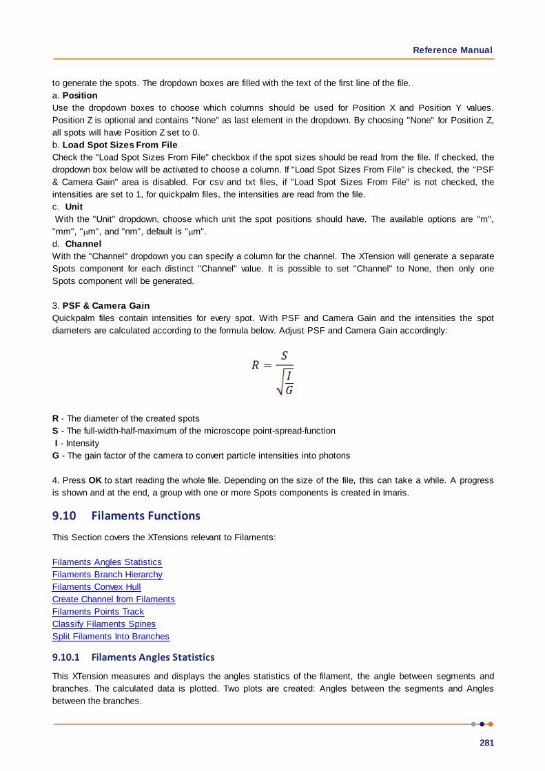
Reference Manual

281

to generate the spots. The dropdown boxes are filled with the text of the first line of the file.

a. Position

Use the dropdown boxes to choose which columns should be used for Position X and Position Y values.

Position Z is optional and contains "None" as last element in the dropdown. By choosing "None" for Position Z,

all spots will have Position Z set to 0.

b. Load Spot Sizes From File

Check the "Load Spot Sizes From File" checkbox if the spot sizes should be read from the file. If checked, the

dropdown box below will be activated to choose a column. If "Load Spot Sizes From File" is checked, the "PSF

& Camera Gain" area is disabled. For csv and txt files, if "Load Spot Sizes From File" is not checked, the

intensities are set to 1, for quickpalm files, the intensities are read from the file.

c. Unit

With the "Unit" dropdown, choose which unit the spot positions should have. The available options are "m",

"mm", " m", and "nm", default is " m".

d. Channel

With the "Channel" dropdown you can specify a column for the channel. The XTension will generate a separate

Spots component for each distinct "Channel" value. It is possible to set "Channel" to None, then only one

Spots component will be generated.

3. PSF & Camera Gain

Quickpalm files contain intensities for every spot. With PSF and Camera Gain and the intensities the spot

diameters are calculated according to the formula below. Adjust PSF and Camera Gain accordingly:

R - The diameter of the created spots

S - The full-width-half-maximum of the microscope point-spread-function

I - Intensity

G - The gain factor of the camera to convert particle intensities into photons

4. Press OK to start reading the whole file. Depending on the size of the file, this can take a while. A progress

is shown and at the end, a group with one or more Spots components is created in Imaris.

9.10 Filaments FunctionsThis Section covers the XTensions relevant to Filaments:

Filaments Angles Statistics

Filaments Branch Hierarchy

Filaments Convex Hull

Create Channel from Filaments

Filaments Points Track

Classify Filaments Spines

Split Filaments Into Branches

9.10.1 Filaments Angles Statistics

This XTension measures and displays the angles statistics of the filament, the angle between segments and

branches. The calculated data is plotted. Two plots are created: Angles between the segments and Angles

between the branches.

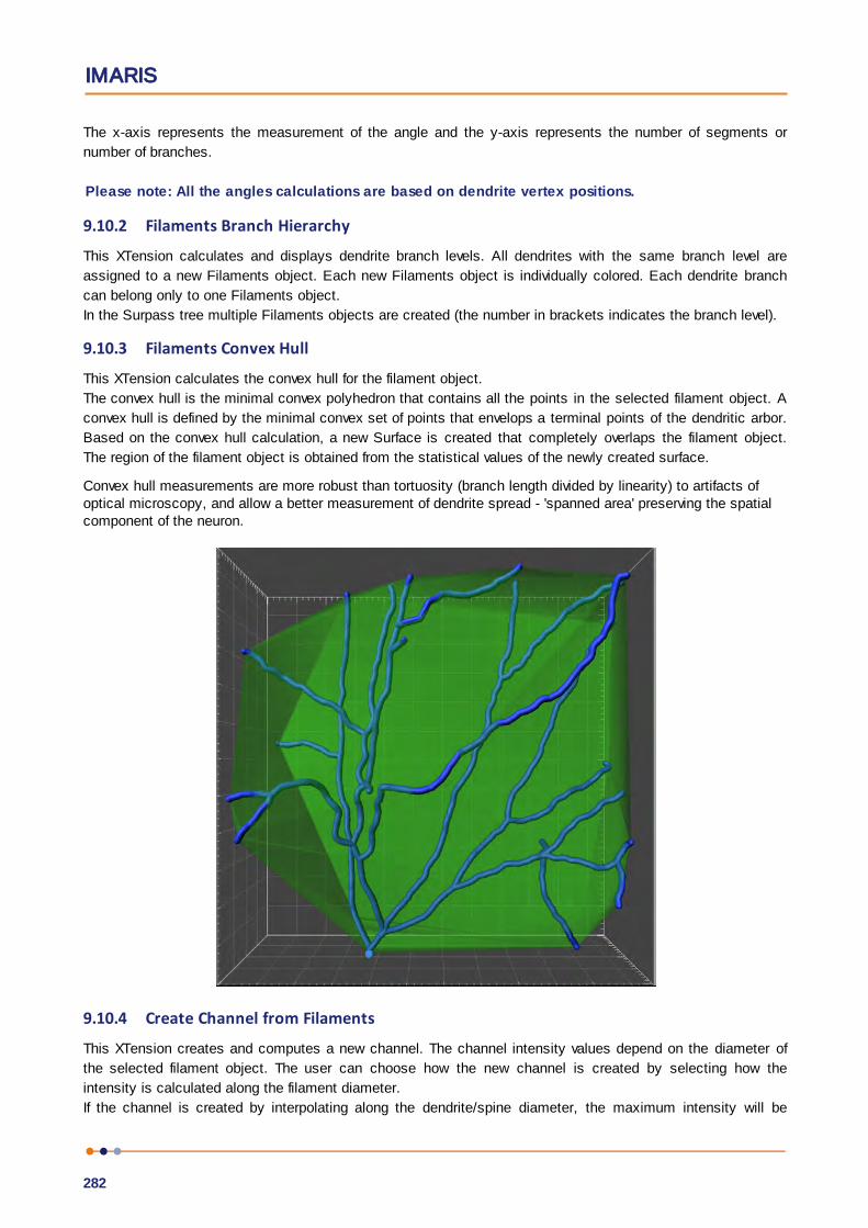
IMARIS

282

The x-axis represents the measurement of the angle and the y-axis represents the number of segments or

number of branches.

Please note: All the angles calculations are based on dendrite vertex positions.

9.10.2 Filaments Branch Hierarchy

This XTension calculates and displays dendrite branch levels. All dendrites with the same branch level are

assigned to a new Filaments object. Each new Filaments object is individually colored. Each dendrite branch

can belong only to one Filaments object.

In the Surpass tree multiple Filaments objects are created (the number in brackets indicates the branch level).

9.10.3 Filaments Convex Hull

This XTension calculates the convex hull for the filament object.

The convex hull is the minimal convex polyhedron that contains all the points in the selected filament object. A

convex hull is defined by the minimal convex set of points that envelops a terminal points of the dendritic arbor.

Based on the convex hull calculation, a new Surface is created that completely overlaps the filament object.

The region of the filament object is obtained from the statistical values of the newly created surface.

Convex hull measurements are more robust than tortuosity (branch length divided by linearity) to artifacts ofoptical microscopy, and allow a better measurement of dendrite spread - 'spanned area' preserving the spatialcomponent of the neuron.

9.10.4 Create Channel from Filaments

This XTension creates and computes a new channel. The channel intensity values depend on the diameter of

the selected filament object. The user can choose how the new channel is created by selecting how the

intensity is calculated along the filament diameter.

If the channel is created by interpolating along the dendrite/spine diameter, the maximum intensity will be

Reference Manual

283

assigned to the voxel at the centre of the filament. If not, the uniform intensity is mapped at the location of the

filament.

Tip: To modify the channel visibility contrast and range, open the Display Adjustment window under

the Edit tab.

9.10.5 Filaments Points Track

This XTension tracks Filament significant points (beginning, dendrite branching and terminal points, spine

attachments and spine branching and terminal points) and plots the track statistics.

It provides several tracking algorithms to choose from. The motion models are used to predict the future

positions of Filament significant points (beginning, dendrite branching and terminal points, spine attachments

and spine branching and terminal points). Based on these predicted positions, the best matches to candidate

Filament significant points can be determined. All of the algorithms except for Connected Components use a

Linear Assignment algorithm and Total Cost function to find the best track connections. The first two algorithms

compute cost based on change in position (distance), while the Autoregressive Expert mode combines the

changes in position and the intensity to compute the total cost.

Brownian Motion

This algorithm models the motion of each of the Filament significant points as a Brownian motion. This model is

appropriate if the Filament significant points perform similar motions to a Brownian motion (the random

movement with very frequent changes in direction and no discernible pattern).

The only prediction applied is that the Filament significant points do not move further than the specified speed

allows, so the maximum speed constrains the distance from one time-point to the next.

Autoregressive Motion

This algorithm models the motion of each of the Filament significant points as an autoregressive AR1 process.

This model is appropriate if the Filament significant points perform any kind of continuous motion. The AR1

model looks back to one time-point and predicts that the Filament significant points will move the same

distance and in the same direction again. The user-specified maximum distance value is the distance in which

the Filament significant points are allowed to deviate from the predicted position. Some changes in direction are

tolerated because of the maximum distance parameter, and because AR1 does not remember farther back than

one time-point.

Autoregressive Motion Expert

This algorithm models the motion of each of the Filament significant points as an autoregressive AR1 process

(see above). It is suitable for the tracing of multiple objects with adjacent or crossing paths, especially if the

neighbouring objects have a stable (but different) intensity. In Autoregressive Motion Expert the algorithm called

Total Cost determines the most appropriate connections for tracks by seeking the lowest Total Cost. In this

case, the Total Cost algorithm combines Intensity Cost and Distance Cost functions (see Intensity Weight

below).

Connected Components

For this algorithm, Filament significant points in adjacent time-points are considered connected if the Filament

significant points’ spheres occupy some of the same space (the spheres would overlap if two time-points were

merged into one). It compares the amount of overlaps between identified objects in the previous frame with

those in the current frame. All objects with an overlap will be assigned the same track ID.

This is the only algorithm that automatically handles lineage (Filament significant points that split or merge). It

will only work with images that have excellent time resolution because the Filament significant points can’t

jump a distance larger than their own size, Max Distance.

Max Distance

IMARIS

284

The value of the Max Distance specifies the maximum distance between a predicted object location and its

actual location for two consecutive time points. This parameter does not allow connections between a Filament

graph and a candidate match when the distance between the predicted future position of the Filament graph

and the candidate position exceeds the maximum distance.

Max Gap Size

An object might fail to be segmented from some time points, which could lead to a Track breaking apart and

the creation of Tracks fractions and create Track fractions.

Instead of creating track fragments, with gaps between undetected objects, the gap-closing algorithm creates

tracks by linearly connecting objects associated with the same track. The time period in which the object’s

connection is automatically established is based on the value defined in the Max Gap Size file.

The Max Gap Size defines the maximum number of the consecutive time points, which are allowed to be

missing in order for the track to be continuous.

Intensity Weight

Based on the information obtained from the measured Filament significant point’s intensity and position, the

Intensity Weight function is used to balance the relative influence of the Intensity and Distance costs. The Total

Cost is determined by combining the Intensity term and Distance term, and minimization of the Total Cost is

used to determine the best track from all feasible ones.

TotalCost = (all connections) DistanceCost + IntensityWeight * IntensityCost

Track Filters

The Track filtering is incorporated into the process. Enter the filtering type to be used in order to classify the

tracks and specify the measurement of the criteria.

As a result of this XTension, a Matlab plot can be created. The plot displays the number of Filament significant

points as a time plot. Each Filament significant point is represented using a special symbol.

In Imaris,a new Spot’s object is created in the Surpass tree.

9.10.6 Classify Filaments Spines

This XTension determines the differences in spine morphology. It classifies spines into the following default

categories: stubby, mushroom, long/thin, and filopodial based on their length, head and neck morphology.

Classification Rule

All detected spines are classified according to the current classification rules. All classification rules are written

as Matlab syntaxes and are fully editable. These are logic statements returning a value of 1 if true and 0 if false.

These rules are applied in order of precedence (i.e. top to bottom). All spines that comply with the first rule (the

first classification rule is true-total spine length is less than 1 m) are set as stubby. For all remaining spines,

the second rule is tested and the process of classification continues.

Any spine that was categorized by the highest rule in the list, is excluded from further classification. Therefore,

a spine can be part of one class only.

Setting the New Rule

You can classify spines according to the default classification rules, or you may create new classification rules

by defining output classes based on the new criteria.

To adjust a classification of the spines morphology into more relevant classes, it is possible to change a set of

classification criteria. In the data set, any detected spine can be selected and measured and then the different

3D features obtained from the spine, can be used for classification. The suitable morphological feature could be

used for setting the new rule.

The list of variables used for setting rules are displayed.

To create or adjust the classification rules combine the spine morphology categories (Spine, Head, Neck,

Reference Manual

285

Ground) with the following variables:

Volume, length, mean/ minimum/ maximum/ width.

Insert variable button

Select the Insert variable button to insert the selected combination of spine morphology and statistical

variables.

Any new rule must be based on Matlab syntaxes. The default classification rules show you a pattern of the

syntax needed to complete these logic statements.

To adjust the rule that controls classification, click on the rule line and enter a new set of classification

criteria.

To change the name of the class, click on the name line and enter a new name.

To remove the selected class, click on the appropriate Remove class button.

In this XTension, the total spine length is divided in 3 parts: ground, neck and head. The spine neck length is

set by default to be 50% of the total spine length. Neck length is measured from the base of the spine head

toward the dendrite. The spine head is 25% of the total spine length. The remaining part of the spine, attached

to the dendrite tree, is set to be 25% of the total spine length. To change the default length ratio enter the new

values in the head/ ground length fields.

Create one Filament

Under the Create One Filament option you can find different outputs.

Create one Filament objet for each class

As a result, in the Surpass tree a new Surpass group is created which is composed of multiple Filament

objects. All spines (and dendrites of the source) categorised in the same class are assigned to the same

Filaments object. Each Filaments object is individually colored.

Create one Filament with custom statistics

As a result, in the Surpass tree a new Filaments object is created. Under the Statistical tab a new variable -

Spine class is added. The spine class is indicated by a numerical value (this value corresponds to the rule

number).

Please note: In both output options every branched spine is replaced with an unbranched one, starting from the

attachment point wherever a branching point is encountered, a new spine is created.

Plot class statistics

A new window plots the selected spine statistics. For each spine class the following statics can be plotted:

count, density, average volume, average length, average mean/ min/max with for total spine, head, neck and

ground.

Variables can be selected interactively.

Density is defined as the total number of selected spines divided by the total length of the dendrite

Add new class button

Select this button and fields for the new classification rule and name are added.

Classify spines

Select this button and the Classify spine XTension is executed.

IMARIS

286

9.10.7 Split Filaments Into Branches

This XTension splits one Filaments object into different Filaments objects. Starting from a common beginning

point and going towards a terminal point, whenever a branching point is encountered a new Filament object is

created. As a result, the newly created Filaments do not have branches and for each branch point, there is only

one beginning and one terminal point. The number of Filaments created is equal to the number of terminals and

branch points of the original Filaments object.

In the Surpass tree a new filament object is created.

9.11 Histogram Equalize LayersThis XTension adjusts the contrast layer by layer by using the image's histogram. Histograms are created for

each layer separately and for the whole image. The XTension enhances the contrast by transforming the

intensity values in each of the layer’s histograms, so that the resulting histogram approximately matches the

whole image histogram.

For more information, please refer to:

http://www.mathworks.ch/help/toolbox/images/ref/histeq.html

The resulting image features the highest possible contrast, uniformly distributed over all the layers.

This method increases the contrast by adjusting the distribution of the intensities on the histogram by

spreading out the most frequent values. This allows for areas of lower local contrast to gain a higher contrast

without affecting the global contrast.

Reference Manual

287

Define the value of the lower limits of intensities. Voxels with an intensity below the entered value are excluded

from this calculation - they are interpreted as background.

9.12 Normalize Time PointsThis XTension adjusts the brightness and contrast of the individual time points in a 4D data set to a uniform

level.

It first computes the mean and standard deviation values of the intensity for all of the time points. Then, it

adjusts the intensities of each time point to match the overall mean and Standard Deviation value.

It adjusts the brightness of all the time points in the data set and each channel independently.

Voxels with intensity below the entered value are excluded from this calculation - they are interpreted as

background.

9.13 Open Object ManagerThis XTension saves, loads or clears single Imaris objects in .mat files.

It can be applied to Spots, Surfaces, Tracks, and Filaments objects and Groups. Groups are saved with all their

content. Only first-level objects (mScene direct children) can be saved.

To change the default location (Matlab), select the Browse button. Select the directory and enter the name for

the file to be saved.

9.14 RGB to GrayThis XTension creates and computes a new gray channel. The intensity values of the gray channel are

calculated as a total weighted sum of the selected channels’ intensities.

The user defines the coefficients of the sum for each channel.

9.15 Smooth TimeThis XTension smoothes the intensity of each voxel along the time dimension. The amount of smoothing is

defined by the Gaussian filter width.

The user specifies the channel and the filter width value.

9.16 Time ProjectionThis XTension projects all channels of a time data set as a single time point. For each voxel the intensity is

computed using a MIP or a mean projection of all time points. The projection mode is defined by the user.

9.17 Time Subtract AverageThis XTension calculates for each voxel a new intensity value, by subtracting the time-averaged intensity value

from the initial intensity. It eliminates all motionless objects since the difference in intensities for motionless

objects are negative values.

There are two options:

1. The user can set all negative values to zero

2. To avoid these negative values and loss of data, any intensity which is zero or negative can be equal to

absolute values

To speed up the processing of 2D time series you can use Image processing - Swap Time and Z before and

after starting the XTension.

IMARIS

288

1. After exchanging the Time and Z dimensions start the XTension.

2. Define the number of slices that should be processed.

3. Select to set Negative values either to zero or to absolute values

4. Run the XTension

5. Finally, under the Image processing menu, select again the Swap Time and Z option

9.18 Tracks FunctionsThis Section covers the XTensions relevant to tracking functions:

Connect Tracks

Plot Angles of selected Tracks

Plot Distance Between Tracks

Plot Length of selected Track

Split Tracks

Translate Tracks

9.18.1 Connect Tracks

For each initial object within the track, this XTension assesses the position at the previous time point.

Then at the previous time, it measures the distance between the calculated position and the positions of all the

other objects. It creates a track connection if the distance between the anticipated object position and any

other object at the previous time point is less than the user specified maximal distance value.

The new connections can be seen under the Edit track tab.

Please note: Two tracks, which track an object through the same time point, cannot be connected.

9.18.2 Plot Angles of selected Tracks

This XTension creates four plots that display the angles statistics of the selected track. The first plot shows the

spatial orientation of the selected track and the following plots are illustrating the XY, XZ and YZ planes.

9.18.3 Plot Distance Between Tracks

This XTension creates four plots that display the distance between the selected track objects and all other

tracks objects that are in the same group. The first plot shows the absolute spatial distance of the selected

track and all other tracks. The following are illustrating planes X, Y and Z distance. The following are illustrating

the distance of the selected track and all other tracks in X, Y and Z planes.

9.18.4 Plot Length of selected Track

This XTension calculates the difference in the object position within the selected track between two consecutive

time points. If the distance between particle (e.g. a vesicle or a cell) positions in two connective time points is

smaller than the entered threshold value, then it is considered as a pause.

As a result, this XTension creates four plots that display the length of the track steps. The first plot shows the

spatial step size of the object within the selected track. The other three plots illustrate the XY, XZ and YZ

planes.

9.18.5 Split Tracks

This XTension splits tracked objects into individual Spots objects.

All objects within one track are assigned to the same Spots object.

Each Spots is individually colored.

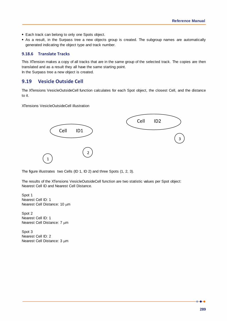
Reference Manual

289

Each track can belong to only one Spots object.

As a result, in the Surpass tree a new objects group is created. The subgroup names are automatically

generated indicating the object type and track number.

9.18.6 Translate Tracks

This XTension makes a copy of all tracks that are in the same group of the selected track. The copies are then

translated and as a result they all have the same starting point.

In the Surpass tree a new object is created.

9.19 Vesicle Outside CellThe XTensions VesicleOutsideCell function calculates for each Spot object, the closest Cell, and the distance

to it.

XTensions VesicleOutsideCell illustration

Cell ID1

Cell ID2

1 2

3

The figure illustrates two Cells (ID 1, ID 2) and three Spots (1, 2, 3).

The results of the XTensions VesicleOutsideCell function are two statistic values per Spot object: Nearest Cell ID and Nearest Cell Distance.

Spot 1Nearest Cell ID: 1Nearest Cell Distance: 10 m



IMARIS

290

Section 10 Fiji

Imaris Fiji compatible plugins are aimed at performing additional image processing and offering a solution for

specific problems with image analysis.

The Imaris Fiji menu allows you to use your current Fiji routines and still continue with your work within Imaris.

The Fiji plugins are integrated into Imaris and can be executed from within the application, enhancing and

extending the functionality of Imaris.

In the Fiji menu you can find a list of plugins organized into a menu structure. Each plugin collection is

displayed as a sub menu on this menu. The plugins and macros are stored and run from the Fiji folder.

Image From Fiji

Image To Fiji

File

Image

Process

Analyze

Plugins

Options...

Help..

Please note: This is not an Fiji tutorial. These Sections describe only the usage of Fiji as an

integrated part of Imaris.

10.1 Fiji-ImarisIn this Section you will learn how to integrate Fuji plugins in Imaris by means of the Fiji menu and how to

establish connections between the Fiji and Imaris.

If you already have Fiji installed, skip down directly to the to the Options… section. If you don't have Fiji

installed, you must install it first. The latest version can be downloaded from the following locations:

Fiji: http://pacific.mpi-cbg.de/wiki/index.php/Downloads

Depending upon your operating system select the appropriate link.

To complete download follow the specific download instructions.

Options...

The first step of integrating the Fiji plugins within Imaris is to specify the folder with the Fiji.exe file. To do that

open the Fiji menu and choose the last item in the list Options...

The Custom Tools window opens. In the field Fiji application either type in the respective path or use the button

Browse.

Specify the Fiji folder and select the .exe file. Click on the OK button.

Reference Manual

291

For Mac users:

/Applications/Fiji.app/Contents/MacOS/fiji-macosx

In the Fiji menu all options are now active.

10.2 Imaris Bridge.jar FileThe downloaded plugins do not include the file needed to run your Fiji plugins in Imaris.

In order to run your Fiji plugins in Imaris you need to install the file, Imaris_Bridge.jar file; which provides the

link between the two applications.

The installation starts automatically as soon as you select a plugin from the list.

The new window appears asking you to install Imaris_Bridge.jar file

You can confirm installation by selecting Yes.

The Imaris_Bridge.jar file is placed in a new subfolder, Imaris, within the Fiji application.

Security Alert window: Depending upon how your computer security is set, you may see a Security

Warning. Select the option Unblock.

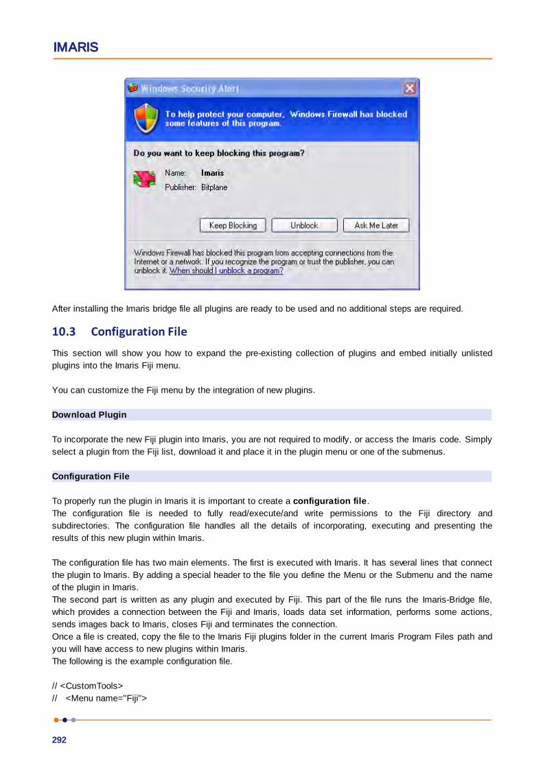
IMARIS

292

After installing the Imaris bridge file all plugins are ready to be used and no additional steps are required.

10.3 Configuration FileThis section will show you how to expand the pre-existing collection of plugins and embed initially unlisted

plugins into the Imaris Fiji menu.

You can customize the Fiji menu by the integration of new plugins.

Download Plugin

To incorporate the new Fiji plugin into Imaris, you are not required to modify, or access the Imaris code. Simply

select a plugin from the Fiji list, download it and place it in the plugin menu or one of the submenus.

Configuration File

To properly run the plugin in Imaris it is important to create a configuration file.

The configuration file is needed to fully read/execute/and write permissions to the Fiji directory and

subdirectories. The configuration file handles all the details of incorporating, executing and presenting the

results of this new plugin within Imaris.

The configuration file has two main elements. The first is executed with Imaris. It has several lines that connect

the plugin to Imaris. By adding a special header to the file you define the Menu or the Submenu and the name

of the plugin in Imaris.

The second part is written as any plugin and executed by Fiji. This part of the file runs the Imaris-Bridge file,

which provides a connection between the Fiji and Imaris, loads data set information, performs some actions,

sends images back to Imaris, closes Fiji and terminates the connection.

Once a file is created, copy the file to the Imaris Fiji plugins folder in the current Imaris Program Files path and

you will have access to new plugins within Imaris.

The following is the example configuration file.

// <CustomTools>

// <Menu name="Fiji">

Reference Manual

293

// <Submenu name="submenu name (e.g. Process)"> -This line is optional (embedding the plugin in the

submenu)

// <Item name="plugin name" icon="Fiji">

// <Command>Fiji::submenu name_plugin name </Command> - Please make sure that the plugin

name is the same as the configuration file name

// </Item>

// </Submenu>

// </Menu>

// </CustomTools>

call("Imaris_Bridge.In", getArgument());

run("plugin name");

call("Imaris_Bridge.Out", getArgument());

call("Imaris_Bridge.Terminate", getArgument());

Save the file, and copy it to the folder:''

Windows: C:\Program Files\Bitplane\Imaris x64 X.X.X\XT\fiji

MAC: /Applications/Imaris\ 9.2.0.app/Contents/SharedSupport/XT/fiji/

Please note: The Imaris version cannot be set differently than the currently running version

Restart Imaris and the newly inserted plugin will appear in the Fiji menu.

Please note: Imaris Fiji compatible plugins are plugins that provide image data as a result.

10.4 Image From FijiTransfer the image to Imaris by selecting the Image From Fiji option.

10.5 Image To FijiTransfer the image to Fiji by selecting the Image to Fiji option.

10.6 Initially Installed PluginsFile

Open

Save

Process

Find Edges

Morphology

Gray Morphology

Sharpen

If you would like to find out more about these plugins, additional information is available in the form the Fiji

website.

IMARIS

294

Analyze

Color inspector 3D

Plugins

LOCI

Bio-Formats Exporter

Bio-Formats Importer

Plugins are not only used to implement new processing functions, they are also used to support reading and

writing file formats, which are not normally supported by Imaris.

Process

Dilate (3D)

Distance Transform (3D)

Erode 3D

Exact Euclidean Distance Transform (3D)

Exact Signed Euclidean Distance Transform (3D)

Gradient (3D)

IFT (3D)

Laplace (3D)

Maximum (3D)

Median (3D)

Minimum (3D)

Particle Analyzer (3D)

Smooth (3D)

For the detail description it is recommend to visit the Fiji website.

There are a lot of examples and tutorials, which could help you to understand the features of these plugins.

http://pacific.mpi-cbg.de/wiki/index.php/Fiji's_Menu

Registration

Correct 3D Drift

Linear Stack Alignment with SIFT

Skeleton

Analyze Skeleton

http://imagejdocu.tudor.lu/doku.php?id=plugin:analysis:analyzeskeleton:start

Skeletonize (2D/3D)

http://imagejdocu.tudor.lu/doku.php?id=plugin:morphology:skeletonize3d:start

Reference Manual

295

10.7 Options...Custom Tools

In Custom Tools you can specify the Fiji folder. Either type in the respective path or use the button Browse.

10.8 Fiji HelpYou can find further Fiji information by clicking on the following link:

http://fiji.sc/wiki/index.php/Fiji

IMARIS

296

Section 11 3D View


Cells 3D View - Cells

Clipping Plane 3D View - Clipping Plane

External Object 3D View - External Object

Filament 3D View - Filament

Frame 3D View - Frame

Surpass Group 3D View - Surpass Group

Light Source 3D View - Light Source

Measurement Point 3D View - Measurement Point

Oblique Slicer 3D View - Oblique Slicer

Ortho Slicer 3D View - Ortho Slicer

Spots 3D View - Spots

Surfaces 3D View - Surfaces

Volume 3D View - Volume

Export Selected Objects...

Delete Selected Objects... Del

Switch View Mode Esc

InMotion InMotion

11.1 CellsImarisCell is an Imaris module designed specifically to identify, segment, track, measure and analyze Cell,

Nucleus and Vesicles in 2D and 3D time-resolved images. ImarisCell provides simultaneous detection,

measurement and analysis of cell objects combined with the interactive identification in the viewing area.

ImarisCell calculates and displays detailed statistics values for all the cell’s components and their tracks.

Interactive image exploration, simultaneous measurement and analysis of the many features in the image

provide quick, accurate, quantitative and reproducible results.

How to Add new Cells?

Select menu 3D - Cells.

The Surpass Tree list is automatically updated and the first window of the Creation Wizard displays in the Cells

- Properties.

For information on cells statistics calculations used refer to Cells.

11.1.1 Creation Wizard

In the first window of the Cell Creation Wizard, you find the algorithm settings. Here, you have to decide, if you

want to load a set of previously stored creation parameters, or to create a new one.

The most convenient way to apply the same creation parameters to different data sets is to use the Load

Parameters option.

Skip automatic creation, edit manually Button

Terminates the creation wizard and activates the manual Cells creation.

If the image data is for a multi-image scene an option to select which source image to be analyzed is available

Reference Manual

297

from the Align to: drop down box.

Depending on the chosen algorithm setting the Creation Wizard could consists of the following major steps:

IMARIS

298

Reference Manual

299

11.1.1.1 Algorithm SettingsNote: If you do not want to use the automatic Cell creation wizard select the Skip automatic creation, edit

manually button.


Terminates the creation wizard and activates the Edit options.

Favourite Creation Parameters

This option lets you use the identical creation parameters for multiple data sets.

The Favourite Creation Parameters option is only available if the set of the creation parameters has already

been saved under the Creation tab using the Remember Parameters button.

Then you can choose to segment a Region of Interest (ROI) only, to create Tracks after objects detection or

to Skip automatic creation.


automatically loaded. The stored parameters contain all of the settings, options, and parameters required for

image segmentation.

Expand the Favourite Creation Parameters drop-down list by clicking on it. The list shows all the creation

parameters sets that have been previously saved, appropriate to the chosen creation wizard. Simply load your

chosen creation parameters set, by clicking on it, and run the wizard as you have preset, without defining all of

the options. On the other hand, you can customize each procedure to your own specific needs by modifying

each part separately - e.g. the same channel settings, with a slightly different threshold.

Algorithm Settings

Depending on the used cell staining techniques and sample preparation Imaris Cell lets you choose from four

different detection types.

You can select to detect Nucleus, Cell and Vesicles , detect Nucleus and Cell , detect

Cell and Vesicles or just to detect Cell .

Segment only a Region of Interest

A Region of Interest (ROI) is a selected sub-region of an image identified for particular processes and analyzes.

Defining and processing ROI allows other parts of an image to be unchanged.

Check this box if you want to segment only a Region of Interest. If option Segment only a Region of Interest is

selected, in the last step of the Creation Wizard only the region of interest is processed.

Process entire Image finally

This option appears only, if Segment only a Region of Interest is checked.

Check this box and in the last step of the Creation Wizard the entire image is processed with the adjusted

parameters (Complete ROI). Un-check this box and only the region of interest is processed.

Track Cells (over Time)

Check this box if you want to track the resulting Cells over time, for details please refer to the Tracking Section.

Cells Wizard Buttons

IMARIS

300

Button Next

Press Next to proceed with the next window of the Creation Wizard.

Button Finish

Click on Finish to calculate the desired Cells and display the Cells objects in the viewing area.

Button Cancel

If you do not want to create the Cell objects click on Cancel.

11.1.1.2 Region of InterestHere you define the region of interest (ROI). Parameters such as width, height and location of the ROI are used

to directly specify the area to work on.

X, Y, Z, Time

Min, Max, Size

Minimum, maximum and Size of ROI coordinate values can be specified either by entering the value in the

value fields or by changing the values by clicking on the up-and down arrows on the right hand side of the value

fields.

Alternatively the location and size of the ROI can be adjusted directly in the viewing area. Size of the ROI:

1. Click on the ROI preview rectangle arrows (change to the pointer mode Select)

2. Drag the arrows to define new coordinates for X ,Y and Z.

Location of the ROI:

1.Click inside the ROI preview rectangle

2. Drag the entire rectangle (with mouse button held) to the chosen image location.

The numbers in the value fields are updated automatically.

Memory Usage:

Display of the memory usage for the image size within the ROI.

Regions of Interest

To select a particular ROI, left-click on its name in the list and the selected ROI will be highlighted within an

image and its properties can be adjusted.

Button Add

Click on this button and a new region of interest appears in the list. To adjust this ROI you have to select the

ROI with a left mouse click.

Button Delete

Select a ROI in the list with a left mouse click and click on this button to delete the ROI.

Total Memory Usage:



Button BackWith Back you return to the previous window of the Creation Wizard.

Button Next

Reference Manual

301


Button FinishClick on Finish to calculate the desired Cells and display the Cell in the viewing area.

Button CancelIf you do not want to create Cells click on Cancel.

11.1.1.3 Nuclei DetectionSource Channel

Select the respective source channel, from which the Nuclei are to be computed.

Nucleus Diameter

The image is processed based on the specified minimum of the object diameter that you have entered. Use

either the automatically given value or set a new measured value.

Advanced Options

Smooth

Check the Smooth option to set up the smoothness of the resulting area. Smoothing applies a Gaussian filter

to the data set.

Smoothing may require a great deal of memory if the data set is very large. Uncheck the check-box or use

smaller ROI if your system does not have enough memory.

If the option Smooth is selected then the Filter Width value should be determined. Use either the automatically

given value or type in a new value in the data field.

Filter Width

The value of the Filter Width determines the Gaussian filter width.

The value is either automatically calculated from the voxel sizes (oriented at the largest voxel dimension) or it

can be directly entered into the numerical field. The value is given by image units and not by the amount of

voxels.


Background Subtraction applies a Gaussian filter to estimate the background intensity value of each voxel. This

variable background is then subtracted from every voxel in the image; Baseline Subtraction is performed.

The width of the Gaussian filter is calculated by subtracting the diameter of the largest sphere that fits into

the Object from the intensity of the original channel.

If the option Background Subtraction is selected then the Sphere Diameter should be determined.

Sphere Diameter


either the automatically given value or set a new measured value. The value of Sphere Diameter should be

slightly larger than the diameter of the largest object expected to be found in the data set.

If the option Background Subtraction is not selected, the Absolute Intensity threshold is performed.

Split Nuclei by Seed Points

Select this option to apply filters to the seed points of the nuclei. Refer to the topic Classify Nuclei Seed Points

for more information on this step.

IMARIS

302



Button NextPress Next to proceed with the next window of the Creation Wizard.



11.1.1.4 Classify Nuclei Seed PointsThe Seed Points filtering is incorporated into the creation process. This tab only appears, if the Split Nuclei by

Seed Points option has been selected.

Filters may allow objects that would interfere with interpretation of results to be removed.

The Filter Type and its values define the section of interest, from this selection, which includes or excludes

objects based on a range of criteria. Select the filter type by selecting a variable from the drop-down list, and

then define the filter values, which will then limit the selection just to those objects that meet the set up

criteria.

In Imaris you can choose two filter values, a Lower and a Higher filter value.

The two filter values separate the data into three regions: above the higher value, below the lower value, and the

region in between. Objects with the relevant properties below the Lower filter value and objects with the

properties exceeding the Higher filter value will be excluded, and only those objects with qualities inside the

defined interval will be considered.

Please note if the value of the Lower filter value is set to be higher than that of the Higher filter

value, the selected objects will be outside the defined interval. Only those objects meeting all the

filter criteria are interactively shown and instantly highlighted in the viewing area. By using multiple

filter types, more than one criterion can be specified for the data analyses.

Filters

Add Button

To add a new filter, click on the button Add and choose one of the Filter Types from the drop-down

menu. The new filter appears in the list.

Delete Button

Select a filter in the list with a left mouse click and click on this button to delete the filter.

Filter Type

Select the filter you want to apply from the drop-down list.

Compact Lower and Upper Threshold

Reference Manual

303

Activating/deactivating the Lower or Upper threshold option is done by clicking on the or button. The

Red button indicates that the threshold option is currently inactive, while the green button indicates an

active threshold.

In order to activate the threshold option, click on the red button. To deactivate the threshold, click on the green

circle again.

Automatic/Manual A/M button

The Automatic/Manual A/M button provides a single interaction point for the direct choice of the threshold value

adjustment.

When the lower/upper threshold values are not activated (the red button ) the corresponding A/M button is

light gray indicating that threshold adjustment is unavailable. When the lower/upper threshold option is

activated (the green button ), the corresponding A/M button turns black.

After the first threshold activation, as a default, an Automatic threshold value is activated . Clicking on the

Automatic/Manual button allows you to switch between an Automatic and a Manual threshold adjustment

mode. The A/M button provides a visual feedback as an indication of the selected threshold adjustment mode.

Clicking on the A/M button changes the appearance of the A/M button form indicating an activated

Automatic threshold to indicating a Manual threshold.

Clicking on the histogram automatically activates a Manual threshold adjustment.

Lower Threshold

Automatic

The initial threshold value is automatically computed.

Manual

Define the threshold by clicking the histogram or by entering the value directly in the data field. Either type in

the value or click the histogram to move the colored line and a reduced/enlarged set of objects is visualized.

Higher Threshold

Automatic


Manual

Define the threshold by clicking the histogram or by entering the value directly in the data field. Either type in

the value or click the histogram to move the colored line and a reduced/enlarged set of objects is visualized.

Histogram

In the histogram the regions above and below the threshold values are displayed in white, while region within

threshold is displayed in yellow. To change the automatically set threshold values, select the option Manual.

By clicking into the histogram you move the colored line and a reduced/enlarged set of objects. To change the

Lower threshold value left-click the histogram and drag the yellow line.

To change the Higher threshold value right click on the histogram and move the line. Move the line to the right

to increase the threshold, while to decrease the threshold move the line to the left. These changes are instantly

visible in the viewing area.

The numerical range of the statistics value (e.g. Quality), the number and percentage of objects selected is

displayed at the bottom of the threshold histogram.

Tip: You can use the Zoom function bar above the histogram to zoom in or out of the histogram

IMARIS

304

display. This may be useful to finely adjust the threshold levels. Right click the range limit bars to set

the range. Use the mouse scroll button to zoom in or out of the selected range.






11.1.1.5 Nuclei ThresholdNucleus Threshold (Absolute Intensity)

In this creation step the Nucleus objects are detected and segmented.

Threshold

Activating/deactivating the Threshold option is done by clicking on the or button. The Red button

indicates that the threshold option is currently inactive, while the green button indicates an active

threshold.


circle again.



adjustment.

When the threshold value is not activated (indicated by the red button ) the corresponding A/M button is light

gray indicating that threshold adjustment is unavailable. When the threshold option is activated (indicated

by the green button ), the corresponding A/M button turns black.

As a default, an Automatic threshold value is activated . Clicking on the Automatic/Manual button allows

you to switch between an Automatic and a Manual threshold adjustment mode. The A/M button provides a

visual feedback as an indication of the selected threshold adjustment mode. Clicking on the A/M button

changes the appearance of the A/M button form indicating an activated Automatic threshold to

indicating a Manual threshold.


Reference Manual

305

Manual

Define the requested threshold by clicking the histogram or by entering the value directly in the data field.

The image’s regions with intensity higher than the set threshold value are Cell objects to be created.

Lower and Upper Threshold

In Imaris you can set two threshold values, Lower and Upper.

The two threshold values separate the data into three regions: above the higher threshold, below the lower

threshold, and the region in between the two values.

Object with values below the Lower Threshold and objects with values exceeding the Higher Threshold will be

excluded and only those objects with quality inside the interval defined by the two threshold values are

considered.

Please note if the value of Lower threshold is set to be higher than the value of Higher threshold the selected

objects will be with outside the interval defined by the two threshold values.

To change the upper and/or lower threshold value(s) you can drag the line(s).

Alternatively, left click in the histogram to set the lower value of the threshold range and right click to set the

upper value of the threshold range.






11.1.1.6 Classify NucleiThe Nuclei classification is incorporated into the creation process under Nuclei Detection Advanced options.

This step allows the removal of objects that would interfere with interpretation of results.




criteria.






IMARIS

306



filter criteria are interactively shown and instantly highlighted in the viewing area.

By using multiple filter types, more than one criterion can be specified for the data analyses.

Filters

Add Button



Delete Button


Filter Type

Select in the drop down list the filter you want to apply.

Filter category

A Category identifies, gathers and summaries a set of statistical values calculations of a particular Object

Type.

Statistical values associated with one object type are grouped in one category. Each category has an


In Imaris there are following Filter Categories: Surface , Surface Tracks , Spots , Spots Tracks ,

Dendrites , Dendrites Tracks , Filament , Filament Tracks , Spines , Spine Tracks , Point ,

Point Tracks , Cell , Cell Tracks , Nucleus , Nucleus Tracks , Vesicle and Vesicles Tracks

.

These buttons allow you to choose the Category and determines the list of displayed statistical values. Clicking

the button selects the corresponding category (the category button turns black) and the list of statistical values

displayed according to the selection.

To remove the category from the list, re-click on the Category button. Re-clicking on the category button de-

selects Category and removes the selected statistical variables from the list (turns the category button into a

light gray color).





active threshold.


circle again.



adjustment.

Reference Manual

307










Lower Threshold

Automatic


Manual

Define the threshold by clicking into the histogram or by entering the value directly in the data field. Either type

in the value or click into the histogram to move the colored line and a reduced/enlarged set of objects is

visualized.

Higher Threshold

Automatic


Manual



visualized.

Histogram




Lower threshold value left click on the histogram and drag the yellow line.










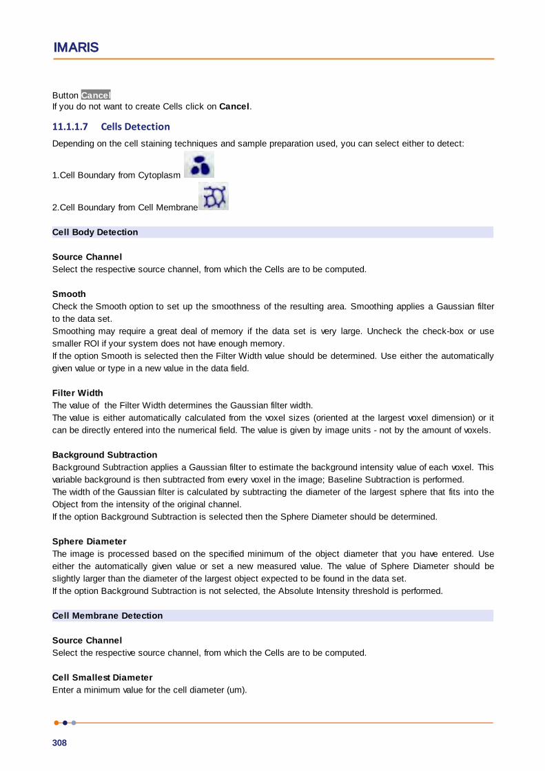
IMARIS

308


11.1.1.7 Cells DetectionDepending on the cell staining techniques and sample preparation used, you can select either to detect:

1.Cell Boundary from Cytoplasm

2.Cell Boundary from Cell Membrane

Cell Body Detection

Source Channel

Select the respective source channel, from which the Cells are to be computed.

Smooth


to the data set.



If the option Smooth is selected then the Filter Width value should be determined. Use either the automatically

given value or type in a new value in the data field.

Filter Width

The value of the Filter Width determines the Gaussian filter width.

The value is either automatically calculated from the voxel sizes (oriented at the largest voxel dimension) or it

can be directly entered into the numerical field. The value is given by image units - not by the amount of voxels.




The width of the Gaussian filter is calculated by subtracting the diameter of the largest sphere that fits into the

Object from the intensity of the original channel.


Sphere Diameter





Cell Membrane Detection

Source Channel

Select the respective source channel, from which the Cells are to be computed.

Cell Smallest Diameter

Enter a minimum value for the cell diameter (um).

Reference Manual

309

Membrane Detail

Set a membrane detail value for the membrane thickness present in the image dataset.

Filter Type

Select the filter type used, either Local contrast (default) or Smooth. Smoothing applies a Gaussian filter to the

data set. A lot of small regions will be detected after this step. These small sub-regions can be fused (merged)

together by adjusting cell threshold values to generate the correct cell detection regions in the Cell Membrane

Threshold step.

11.1.1.8 Cells ThresholdCell Body Detection Threshold (Absolute Intensity)

When Cell Body Detection has been selected the following options are available in this creation step in which

the Cell objects are detected and segmented.

Threshold

Activating/deactivating the Threshold option is done by clicking on the or button. The Red button


threshold.


circle again.



adjustment.

When the threshold value is not activated (indicated by the red button ) the corresponding A/M button is light

gray indicating that threshold adjustment is unavailable. When the threshold option is activated (indicated

by the green button ), the corresponding A/M button turns black.

As a default, an Automatic threshold value is activated . Clicking on the Automatic/Manual button allows

you to switch between an Automatic and a Manual threshold adjustment mode. The A/M button provides a

visual feedback as an indication of the selected threshold adjustment mode. Clicking on the A/M button

changes the appearance of the A/M button form indicating an activated Automatic threshold to

indicating a Manual threshold.


Manual

Define the requested threshold by clicking into the histogram or by entering the value directly in the data field.

The image’s regions with intensity higher than the set threshold value are Cell objects to be created.







considered.

IMARIS

310






Split Touching Cells

Don't Split

When this option is selected the Split Cells’ algorithms are not activated.

One Nucleus per Cell

When the automatic algorithm does not properly segment the cells, creating cell objects containing two or

more nuclei, this option can be used. When activated, this option performs a separation of cells, resulting in

every single cell containing only one Nucleus. The algorithm used for this separation is the Marker Controlled

Watershed.

Split by Seed Points

This option supports the separation of two or more of the Cells objects,that have been identified as one, in the

Threshold step.

The Split Cells method for segmentation in Imaris starts with defined seed points. You use the Cells as seed

points for the Cells segmentation that will be performed in the next steps. During the process, the region around

each seed point grows until it reaches the border.

Seed Points Diameter

Type in the estimated diameter of a seed point.

Nuclei Options

Expand Cell on Nucleus

This option defines the voxel set which is assigned, in the segmentation step, as a boundary of the Cell object.

Areas of the image that have been initially segmented as Cells are expanded outside the original borders, to

include a set of voxels which are defined in the segmentation step as Nuclei.

Resulting in a union between the set of voxels defining the Cells and the set of voxels initially defined as Nuclei.

Erase Nucleus outside Cell

This option defines the voxel set which is assigned as a boundary for the segmented Nucleus.

Any parts of Nuclei that are segmented outside the Cell object is removed from the preview area, leaving only

set of voxel assigned as Nucleus within the Cell object. This means that the segmented Nuclei boundary will be

reduced to the voxel set defined as the Cell object.

Reference Manual

311






11.1.1.9 Cell Membrane Threshold

Cell Membrane Threshold

When the Cell Membrane Detection type has been selected the following options are available for Cell

Membrane Threshold Detection:

In the previous Cells Detection step, there are two filter options "Local Contrast" and "Smooth" that set the

available cell membrane threshold settings.

For the "Local Contrast" filter, two threshold values can be adjusted to fuse the basic regions. The first value is

Intensity which is the average intensity value of the border segment of the regions on the smooth image. The

histogram of the Intensity represents the values of all border segments. By adjusting the Intensity value, the

border segment whose value is below the threshold is removed so that its connected two basic regions are

fused together. By adjusting the Intensity value threshold, the small sub-regions which are located on the

background region can be easily fused together to generate a better background region. The second value is

Quality which is the value of the border segment of the fused regions which are generated by adjusting the first

value Intensity on the filtered image. So the Quality value is based on the fused regions generated by adjusting

the Intensity.

For the "Smooth" filter, one threshold value can be adjusted to fuse sub-regions. The Quality is the value of the

border segment of the basic regions on the smooth image. By adjusting the Quality value threshold, the basic

regions can be fused together to generate the better results.

11.1.1.10 Classify CellsThe Cell object classification is incorporated into the creation process.


IMARIS

312




criteria.









filter types, more than one criterion can be specified for data analysis.

Filters

Add Button



Delete Button


Filter Type





active threshold.


circle again.



adjustment.










Reference Manual

313

Lower Threshold

Automatic


Manual


in the value or click the histogram to move the colored line and a reduced/enlarged set of objects is visualized.

Higher Threshold

Automatic


Manual



Histogram

In the histogram the regions above and below the threshold values are displayed in white, while the region within


By clicking the histogram you move the colored line and a reduced/enlarged set of objects. To change the















11.1.1.11 Vesicles DetectionSelect this option to start the automatic creation process for Vesicles.

The drop-down list shows the types of Vesicles that will be detected in the creation process.

IMARIS

314

To detect the additional vesicles types

To add a new Vesicles type, click on the button and choose the name. The new Vesicles type name appears in

the list.

1. Click on the Add New Type Button

2. Enter a Vesicle name in the Vesicles name field

3. The new Vesicles type name appears in the list

4. Select the Source Channel

5. Define the Estimated Diameter

6. Decide on the Background Subtraction

Vesicle Name

This field allows you:

1. To enter the name for a newly added vesicle type or

2. To edit a name already defined

Source Channel

Select the respective source channel, from which the Vesicles are to be computed.

Estimated Diameter

Objects with size smaller than the specified Estimated Diameter are not detected.


If checked, the background will be removed prior to Vesicle detection. Technically the background subtraction

is used to smooth the image. The intensity equals the Gaussian filtered channel (Gaussian filtered by 3/4)

minus the intensity of the original channel Gaussian filtered by 8/9 of sphere radius.

Different Vesicles Sizes (Region Growing)

The following options only appears, when the Different Vesicles Sizes (Region Growing) box is checked.

The region method for segmentation in Imaris starts with defined seed points. You use Vesicles as seed points

for the region growing that is performed. During the region growing process around each seed point the region

grows until a border stops the growing.

Vesicles Regions from

Absolute Intensity

Local Contrast

You can set the border using the Absolute Intensity or the Local Contrast as criteria. In both cases as next

step the selected channel is displayed in the viewing area.

Local Contrast

This option should only be used when the Absolute Intensity method does not properly segment all objects.

Please note: Local Contrast applies a Gaussian filter in order to estimate the intensity value of each voxel.

Baseline Subtraction is then performed by subtracting the variable background from every voxel in the image.

As a result, it uses more memory than the Absolute Intensity method.

Gaussian Smoothing replaces the voxel intensity value with a newly calculated value. The new value is a

weighted sum, defined using a Gaussian function, of the voxel and it neighbouring voxels.

The degree of the smoothing is directly dependent on the shape of this kernel, which in turn is a function of the

Reference Manual

315

standard deviation. A Gaussian kernel is a symmetric bell shaped curve.

Absolute Intensity Local Contrast

Add New Type Button

To add a new vesicles types, click on the button Add and choose the appropriate settings.

Delete Button

Select a Vesicles type in the list and click on this button to delete it.






11.1.1.12 Classify VesiclesVesicle filtering is incorporated into the creation process.

Click on the drop-down list and select the required Vesicle type to be classified.


IMARIS

316


objects based on a range of criteria.

First select the Vesicle type. Then select the filter type by selecting a variable from the drop-down list, and

finally define the filter values, which will then limit the selection just to those objects that meet the set up

criteria.









filter types, more than one criterion can be specified for the data analysis.

Filters

Add Button



Delete Button


Filter Type


Filter category


Type.






.



displayed according to the selection.



light gray color).



Reference Manual

317



active threshold.


circle again.



adjustment.







Clicking the A/M button changes the appearance of the A/M button form indicating an activated



Lower Threshold

Automatic


Manual



visualized.

Higher Threshold

Automatic


Manual



visualized.

Histogram










IMARIS

318









11.1.1.13 Vesicle RegionsThis tab only appears, if Different Vesicle Sizes (Region Growing) is checked.

Vesicle Regions

The working channel is visualized in the viewing area, the histogram is displayed in the properties area. Regions

above the threshold are displayed in white, regions below threshold are displayed in black. Depending on the

previously selected detection method (Absolute Intensity or Local Contrast) refer to Absolute Intensity or Local

Contrast.

Threshold



adjustment.







Absolute Intensity

Automatic

In the working channel a copy of the intensity histogram of the source channel is displayed. Regions above the

threshold are displayed in white. Now you adjust the threshold of the working channel. Edit the data field or

adjust the threshold manually using the mouse (click & drag the line in the histogram). In the next step the

regions will grow until they fill the white regions and reach the border.

Local Contrast

Reference Manual

319

Automatic

In the selected channel the regions with a local contrast brighter than the background are displayed in white.

Now you adjust the threshold value of the local contrast channel. Edit the data field or adjust the threshold

manually using the mouse (click & drag the line in the histogram). In the next step the regions will grow until

they fill the white regions and reach the border.

Diameter from

Region Volume

The Vesicles radius is calculated from the region volume (the region volume and the Vesicles volume are

equal).

Create Color Coded Region Channel

Additionally the Vesicles the Region Channel is displayed. Each region has a different color.

Region Border

The radius of the calculated Vesicles is the smallest distance from each Vesicles center to the region border.


Button Back

With Back you return to the previous window of the Creation Wizard.

Button Next


Button Finish

Click on Finish to calculate the desired Cells and display the Cells objects in the viewing area.

Button Cancel

If you do not want to create Cells objects click on Cancel.

11.1.1.14 Tracking CellsTracking allows objects to be traced throughout sequential frames of a time data set, so each object maintains

a unique identity in the output measurements.

Tracking the Nucleus and Vesicle objects with respect to the inertial image coordinates is less significant than

tracking their relative motion within the cell.

In order to cope with the spatial position of Nuclei and Vesicles within the Cell, the concepts of relative tracking

are required.

Tracking of Nuclei and Vesicles objects is presented in relative terms of their parent Cell objects, rather than

their real coordinates on the screen.

Since the Cell object itself can be moving (relative to the inertial image reference frame), the tracking of Nuclei

and Vesicle is relative to the parent Cell of a specified reference point.

The position of the Nuclei and Vesicle objects is specified as a relative distance from a reference point. This

reference point is the Cell object center of mass.

The position of the individual Nuclei and Vesicles objects is calculated using two types of information. One is

the absolute position of the selected object in terms of the inertial image reference coordinates and the other is

the absolute position of the parent Cell object center. The relative Nuclei and Vesicles object’s position is

calculated by subtracting these two positional differences and is then tracked.

This concept of relative tracking allows direct measurements and statistical data comparison between moving

IMARIS

320

cells to be calculated.

Algorithm

Brownian Motion

This algorithm models the motion of each object (Nuclei or Vesicles) as a Brownian motion. This model is

appropriate if the object performs similar to a Brownian motion (the random movement of objects with very

frequent changes in direction and no discernible pattern).

The only prediction applied is that the object does not move further than the specified speed allows, so the

maximum speed constrains the distance from one time-point to the next.


This algorithm models the motion of each cell object (Nuclei or Vesicles) as an autoregressive AR1 process.

This model is appropriate if the object performs any kind of continuous motion. The AR1 model looks back to

one time-point, and predicts that the object will move again the same distance and in the same direction. The

user-specified Maximum Distance value is the distance in which the object is allowed to deviate from the

predicted position. Some changes in direction are tolerated because of the maximum distance parameter, and

because AR1 does not remember farther back than one time-point.


This algorithm models the motion of each cell object (Nuclei or Vesicles) as an autoregressive AR1 process

(see above). It is suitable for tracing of multiple objects with adjacent or crossing paths, especially if the

neighboring objects have a stable (but different) intensity. In Autoregressive Motion Expert the algorithm called



below).


For this algorithm, objects in adjacent time-points are considered connected if the object spheres occupy some

of the same space (the spheres would overlap if two time-points were fused into one). It compares the amount

of overlaps between identified objects in the previous frame with those in the current frame. All the object with

the overlap will be assigned the same track ID.

Connected Components and Lineage are the only algorithms that automatically handle lineage (objects that

fuse or fragment). It will only work with images that have excellent time resolution, because the object cannot

ever jump a distance larger than its own size.

Lineage

The Lineage model is intended for events such as cell division in which the splitting of objects is to be

analyzed. This algorithm models the motion of each object (Nuclei or Vesicles) as an autoregressive AR1

process (refer to Autoregressive Motion above). The object data is then compared so that only the objects that

undergo splitting are connected, and assigned the same track ID. Objects that pass in close proximity, or

overlap, are not associated. This is in contrast to connected components, where any objects that overlap are

determined and considered connected.

Maximum Overlapping

For a cell at time point t the overlap with all cells at the previous time point t-1 is computed and the cell is

linked to that cell from the previous time point with which it has the largest overlap. The link is only created if

the ratio of the volume of the smaller of the two linked cells to the larger is greater than the "maximum

overlapping ratio".

Parameters

Reference Manual

321

Max Distance Cell

The value of the Max Distance specifies the maximum distance that a track Cell object could possibly move

between two consecutive time points. This parameter disallows the connection between a Cell and a candidate

match if the distance between the predicted future position of the Cell and the candidate position exceeds the

maximum distance.

Max Relative Distance Nucleus

The value of the Max Distance specifies the maximum distance that a track Nucleus could possibly move

between two consecutive time points, relative to the parenting Cell center of mass.

Max Relative Distance Vesicles

The value of the Max Distance specifies the maximum distance that a track Vesicles could possibly move


Options

It can happen that the object segmentation fails for some time points. This can break a Track apart into two

Tracks. A gap-closing algorithm links track segment ends to track segment starts in order to recover tracks

that were interrupted by the temporary disappearance of particles.

Close Gap

Select this option and the gap-closing algorithm is implemented.

Max Gap Size


the creation of Tracks fractions.


tracks by linearly connecting objects associated with the same track. The time period in which the objects

connection is automatically established is based on the value defined in the Max Gap Size value.


missing in order to a track to be continues.

Fill the gaps with all detected objects

This algorithm allows tracks to be continued, even if the object was not detected in periods of up to two

consecutive time points along the trajectory. If this option is selected the algorithm performs the optimization of

the object expected position for the particular time point. The track is generated by connecting objects

assuming their optimized expected positions.

Track Nuclei and Vesicles

Select this option to track nuclei and vesicles. Refer to Tracking Nuclei and Vesicles for information (This option

is only available if the relevant detection algorithm has been selected).


Button Back

IMARIS

322





Track

Select track to select a complete track. Refer to Tab Edit Tracks for editing information.

11.1.1.15 Classify Cells TracksTracks filtering is incorporated into the creation process. This tab only appears, if Track Cells (over Time) is

checked (Algorithm).





criteria.










Filters

Add Button

To add a new filter, click on the button Add and choose one of the Filter Types from the drop-down menu. The

new filter appears in the list.

Delete Button


Filter Type


Filter category


Type.



Reference Manual

323




.



is displayed according to the selection.



light gray color).





active threshold.


circle again.



adjustment.










Lower Threshold

Automatic


Manual



visualized.

Higher Threshold

Automatic


Manual


IMARIS

324


visualized.

Histogram


the threshold is displayed in yellow. To change the automatically set threshold values, select the option

Manual. By clicking into the histogram you move the colored line and a reduced/enlarged set of objects. To

change the Lower threshold value left click on the histogram and drag the yellow line.




The numerical range of the statistics value (e.g. Quality), the number and percentage of objects selected (e.g.

Tracks) is displayed at the bottom of the threshold histogram.




Surfaces Wizard Buttons

Button Back



Button Finish

Click on Finish to calculate the desired Surfaces and display the Surfaces in the viewing area.

Button Cancel

If you do not want to create Surfaces click on Cancel.

11.1.1.16 Tracking Nuclei and VesiclesTracking allows objects to be traced throughout sequential frames of a time data set, so each object maintains

a unique identity in the output measurements.

Tracking the Nucleus and Vesicle objects with respect to the inertial image coordinates is less significant than

tracking their relative motion within the cell.

In order to cope with the spatial position of Nuclei and Vesicles within the Cell, the concepts of relative tracking

are required.

Tracking of Nuclei and Vesicles objects is presented in relative terms of their parent Cell objects, rather than

their real coordinates on the screen.

Since the Cell object itself can be moving (relative to the inertial image reference frame), the tracking of Nuclei

and Vesicle is relative to the parent Cell of a specified reference point.

The position of the Nuclei and Vesicle objects is specified as a relative distance from a reference point. This

reference point is the Cell object center of mass.

The position of the individual Nuclei and Vesicles objects is calculated using two types of information. One is

the absolute position of the selected object in terms of the inertial image reference coordinates and the other is

the absolute position of the parent Cell object center. The relative Nuclei and Vesicles object’s position is

calculated by subtracting these two positional differences and is then tracked.

This concept of relative tracking allows direct measurements and statistical data comparison between moving

Reference Manual

325

cells to be calculated.

Track

Track Nuclei

Select this option to apply the required algorithm and parameters to Nuclei.

Track Vesicles

Select this option to apply the required algorithm and parameters to Vesicles.

Algorithm

Brownian Motion

This algorithm models the motion of each object (Nuclei or Vesicles) as a Brownian motion. This model is

appropriate if the object performs similar to a Brownian motion (the random movement of objects with very

frequent changes in direction and no discernible pattern).

The only prediction applied is that the object does not move further than the specified speed allows, so the



This algorithm models the motion of each cell object (Nuclei or Vesicles) as an autoregressive AR1 process.

This model is appropriate if the object performs any kind of continuous motion. The AR1 model looks back to

one time-point, and predicts that the object will move again the same distance and in the same direction. The

user-specified Maximum Distance value is the distance in which the object is allowed to deviate from the

predicted position. Some changes in direction are tolerated because of the maximum distance parameter, and

because AR1 does not remember farther back than one time-point.


This algorithm models the motion of each cell object (Nuclei or Vesicles) as an autoregressive AR1 process

(see above). It is suitable for tracing of multiple objects with adjacent or crossing paths, especially if the

neighboring objects have a stable (but different) intensity. In Autoregressive Motion Expert the algorithm called



below).


For this algorithm, objects in adjacent time-points are considered connected if the object spheres occupy some

of the same space (the spheres would overlap if two time-points were merged into one). It compares the amount

of overlaps between identified objects in the previous frame with those in the current frame. All the object with

the overlap will be assigned the same track ID.

Connected Components and Lineage are the only algorithms that automatically handle lineage (objects that

diverge). It will only work with images that have excellent time resolution, because the object cannot ever jump

a distance larger than its own size.

Lineage


analyzed. This algorithm models the motion of each object (Nuclei or Vesicles) as an autoregressive AR1

process (refer to Autoregressive Motion above). The object data is then compared so that only the objects that

undergo splitting are connected, and assigned the same track ID. Objects that pass in close proximity, or

overlap, are not associated. This is in contrast to connected components, where any objects that overlap are

determined and considered connected.

IMARIS

326

Parameters

Max Distance Cell

The value of the Max Distance specifies the maximum distance that a track Cell object could possibly move

between two consecutive time points. This parameter disallows the connection between a Cell and a candidate

match if the distance between the predicted future position of the Cell and the candidate position exceeds the

maximum distance.

Max Relative Distance Nucleus

The value of the Max Distance specifies the maximum distance that a track Nucleus could possibly move


Max Relative Distance Vesicles

The value of the Max Distance specifies the maximum distance that a track Vesicles could possibly move


Options

It can happen that the object segmentation fails for some time points. This can break a Track apart into two

Tracks. A gap-closing algorithm links track segment ends to track segment starts in order to recover tracks

that were interrupted by the temporary disappearance of particles.

Close Gap

Select this option and the gap-closing algorithm is implemented.

Max Gap Size















Button Next

Reference Manual

327




11.1.1.17 Classify Nuclei and Vesicles TracksTracks filtering is incorporated into the creation process. This tab only appears, if Track Cells (over Time) is

checked (Algorithm).





criteria.










Filters

Add Button

To add a new filter, click on the button Add and choose one of the Filter Types from the drop-down menu. The

new filter appears in the list.

Delete Button


Filter Type


Filter category


Type.






IMARIS

328

.






light gray color).





active threshold.


circle again.



adjustment.










Lower Threshold

Automatic


Manual



visualized.

Higher Threshold

Automatic


Manual



visualized.

Histogram

Reference Manual

329



Manual. By clicking into the histogram you move the colored line and a reduced/enlarged set of objects. To






Tracks) is displayed at the bottom of the threshold histogram.





Button Back



Button Finish


Button Cancel


11.1.1.18 Complete ROIThis tab only appears, if Process entire Image finally is checked (Algorithm).

Region of Interest

The parameters you have set up will now be used to compute Spots (and Tracks) for the entire data set.

Depending on the size of the data set this may take a while.


Button Back


Button Finish

Click on Finish to end the calculation and display the results in the viewing area.

Button Cancel


IMARIS

330

11.1.2 Tab Settings

On Tab Settings you can choose the rendering methods and adjust the rendering quality to produce faster

performance of the display.

Object Type

A choice of Object types is presented. For time series images the choice of the Object Type is in the drop-

down list. After choosing the Object type, a selection of the Setting Tab is listed.

Cell/Nuclei

Cell Tracks

Nuclei Tracks

Vesicle Type and Tracks

Volume and Slicer Display

The option Volume Display is used to identify the different objects and distinguish them from the surrounding

by visualizing the volume around a created object. It extracts a subset of the volume data set by using the

specified axis-aligned limits.

The border around each object is defined independently and corresponds to the regions equal to bounding box

of the created object.

MIP

In the Maximum Intensity Projection mode only the point with maximum intensity of all layers along the viewing

direction displayed. If your data set has more then one channel, the combination color is displayed.

Shaded Volume

This option displays the subvolume around a certain object in the shaded volume mode. In this mode, all values

along the viewing direction including their transparency are used for the calculation.

Slicer display options are described in the Cell/Nuclei section.

11.1.2.1 Cell/NucleiCell and Nuclei Style

Cell visible

This option shows or hides the Cell objects in the viewing area.

Nucleus visible

This option shows or hides the Nucleus objects in the viewing area.

Slicer Display

Slicer Direction

The Slicer display represents an orthogonal plane (orthogonal to the coordinate axis of the data set) that can be

moved within the data set. Three orthoslicer planes show their intersection with a plane perpendicular to two of

the coordinate axes

Change the slice direction if required by selecting the appropriate XYZ plane option.

The position of slices can be changed in the viewing area. Switch the pointer to the Select mode and then click

on the plane and drag it to a new position. A series of slices is shown below for XY Slicer direction, Border

Reference Manual

331

rendering and Solid color region rendering.

The check buttons labeled as XY, XZ and YZ direction, are used to select the visibility of the corresponding

slice. The Oblique option represents a plane that can be freely moved and rotated within the data set and

allows the user to look inside any object. The Oblique Slicer (shown below) consists of a colored frame with a

white double rod in the middle.

The position of the Oblique Slicer can be changed. Choose the pointer mode Select, highlight the Oblique

Slicer in the viewing area and click on the bigger diameter rod. It will appear highlighted as it is selected,

allowing you to move it and to set the Oblique Slicer to the required position.

The Oblique Slicer can be rotated around the x-, y-, and the z-axes. In the Select mode click the smaller

diameter rod and it will be highlighted as it is selected. To rotate the Oblique Slicer, move the smaller rod.

Border Rendering

Border rendering can be a useful visualization tool- it displays the cell borders that have been calculated during

the cell creation process. This can be seen in the following image compared to the previous image without

Border rendering. The width of the border may be changed using the Border width slider bar.

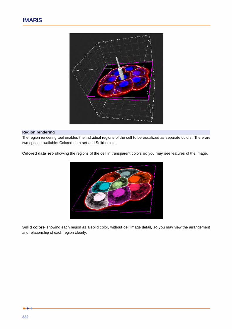
IMARIS

332

Region rendering

The region rendering tool enables the individual regions of the cell to be visualized as separate colors. There are

two options available: Colored data set and Solid colors.

Colored data set- showing the regions of the cell in transparent colors so you may see features of the image.

Solid colors- showing each region as a solid color, without cell image detail, so you may view the arrangement

and relationship of each region clearly.

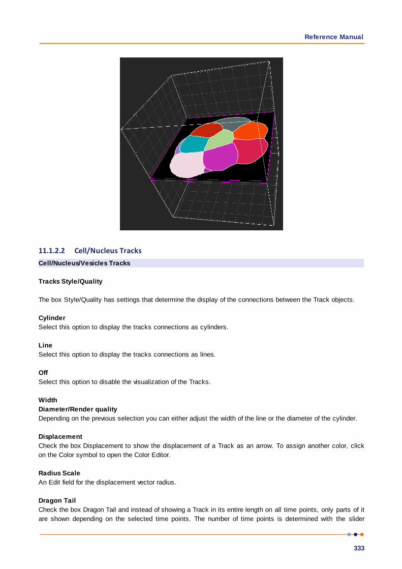
Reference Manual

333

11.1.2.2 Cell/Nucleus TracksCell/Nucleus/Vesicles Tracks

Tracks Style/Quality

The box Style/Quality has settings that determine the display of the connections between the Track objects.

Cylinder

Select this option to display the tracks connections as cylinders.

Line

Select this option to display the tracks connections as lines.

Off

Select this option to disable the visualization of the Tracks.

Width

Diameter/Render quality

Depending on the previous selection you can either adjust the width of the line or the diameter of the cylinder.

Displacement

Check the box Displacement to show the displacement of a Track as an arrow. To assign another color, click

on the Color symbol to open the Color Editor.

Radius Scale

An Edit field for the displacement vector radius.

Dragon Tail

Check the box Dragon Tail and instead of showing a Track in its entire length on all time points, only parts of it

are shown depending on the selected time points. The number of time points is determined with the slider

IMARIS

334

position.

Slider

The Dragon Tail length can be adjusted using the slider. The slider determines the number of time points in the

length of the Dragon Tail.

11.1.2.3 Vesicle Type and TracksVesicles Style/Quality

On the tab Settings you can adjust the rendering style or quality.

Center Points

This option displays the Vesicles as center points.

Off

Select this option to disable the visualization of the Vesicles.

Sphere

Select this option to display the Vesicles as spheres.

Radius Scale box

The size of the Vesicles can be changed via the Radius Scale box.

The Render QualityThe Render Quality is adjustable using the slider. When the number of Vesicles is very large, adjust the Render

Quality, to produce a faster display performance.


The box Style/Quality has settings that determine the display of the connections between the Track objects.

Cylinder

Select this option to display the tracks connections as cylinders.

Line

Select this option to display the tracks connections as lines.

Off


Width

Diameter/Render quality

Depending on the previous selection you can either adjust the width of the line or the diameter of the cylinder.

Displacement

Check the box Displacement to show the displacement of a Track as an arrow. To assign another color, click

on the Color symbol to open the Color Editor.

Radius Scale

An edit field for the displacement vector radius.

Reference Manual

335

Dragon Tail


are shown depending on the selected time points. The number of time points is determined with the slider

position.

Slider

The Dragon Tail length can be adjusted using the slider. The slider determines the number of time points in the

length of the Dragon Tail.

11.1.3 Tab Rebuild

Rebuild

Imaris stores the list of operations and the mapping of parameters. Select from the list, which step of the Cell

Creation Wizard you want to re-enter.

For details please refer to Section:

Menu 3D View - Cells - Algorithm

Menu 3D View - Cells – Tracking

Rebuild Objects Button

Click on this button to start the rebuild.

Creation Parameters

The Creation Wizard saves parameters and processing instructions so that the Cell computation can be

repeated for the same region, a different region, or the entire image. The Creation Parameters are listed as the

table.

Store Parameters for the Batch

The Store Parameters for the Batch button allows you to save the complete set of the creation parameters and

all relevant settings shown in the list. In the Store Creation Parameter window, enter a descriptive name for your

creation parameters and select the required store location.

There are two options to store your creation parameters:

Arena

Favorite Creation Parameters

Arena

When you select this option a new Arena item is automatically created within the Arena view. The Arena view is

updated, a new item, Creation Parameters, is created and displayed.

Once stored, Imaris Batch applies the creation parameters set to all images within the selected Group.


To help you organize and find your most used creation parameters more easily, we advise you to store them by

selecting the Favorite Creation Parameters option.

When you select this option the Creation Parameter file is automatically added to the list that is displayed

under the Edit/Preference/ Favorite Creation Parameters. This option allows you to use the creation parameters

in future on another data set. These saved parameters can then be imported and re-used on any new data set

should you wish to perform an identical analysis sequence. This option is also useful for sharing the parameters

with other users to allow them to perform the same analysis on their own data sets.

IMARIS

336

Within the 3D View view storing allows the parameters to be reused or modified. In addition, this option is useful

to create and share the creation parameters with other people and allow them to perform their own analysis on

it.

Once you have saved the creation parameters, you can reuse them in any new creation wizard. All the settings

and values required to apply the same parameters to the new data set are automatically loaded and available

as a Load Parameter option in the creation wizard.



Click on the Store Parameters for the Batch button opens the Store Creation Parameter window.

Store Creation Parameter

Refer to Store Creation Parameters

11.1.4 Tab Edit

Once the Cell creation wizard is completed, use these buttons for manual editing of the Cell objects. It allows

you:

1. To import Surfaces or Spots and incorporate them in the Cells analysis.

2. To export objects from the Cells.

3. To clear the selection or delete all selected component of the cell object.

Import

Import Surface to Cells

To import the Surface as the Cell or the Nuclei Objects, click on this button. The window, Import to Cells

Objects, will appear.

Import Spots to Vesicles

To import the Spots as the Vesicles, click on this button. The window, Import to Cell Object, will appear.

Import to Cell Object window

Choose one of the objects from the drop-down list. Choose how the selected object type is to be imported and

specify the selection and the time.

The Surface can be imported either as the Cell or the Nuclei.

The Spots can be imported only as the Vesicles.

Import as

Choose to import the object either as a new Vesicle type or as a previously detected Vesicle type.

To import the Spots object as an already segmented Vesicle type, please select the correct name from the

drop-down list.

Selection

The user can decide either to import the Selection or the All objects of the specified component.

Reference Manual

337

Time

The time point of the object selected can be imported either as the Current time point or the All time

points.

Export

Selection

The Selection checkbox is used to export only the currently selected object.

All Timepoints

The All Timepoints checkbox is used to export the object for all time points.

Export Cells to Surface

With a click on this button you export the Cell objects to a Surface object. The Surpass Tree list is

automatically updated with the new item with the automatically generated name Cells n Cell Export. The

exported objects can be then manually edited.

Export Nuclei to Surface

With a click on this button you export the Nuclei objects to a Surface object. The Surpass Tree list is

automatically updated with the new item with the automatically generated name Cells n Nucleus Export.

The exported objects can be then manually edited.

Export Vesicles to Spots

With a click on this button you export the Vesicles to a Spots object. The Surpass Tree list is automatically

updated with the new item with the automatically generated name Cells n Vesicles Export. The exported

objects can be then manually edited.

Full Export

With a click on this button you export all the Cell objects. The Cell and Nuclei objects are exported to

Surface, while the Vesicles objects are exported to Spots.

The Surpass Tree list is updated and three new surpass objects are generated (two Surface items and one

Spots item) with the automatically generated names Cells n object-name Export. Pressing this button has

the same effect as pressing the three buttons above.

Selection

Clear Button

Click this button to clear the current object selection.

Delete Button

Click on this button to delete all the currently selected components.

All actions in the Draw , Edit and Edit Tracks tabs can be Undone/Redone by selecting the

Undo/Redo command or by pressing Ctrl+Z/Ctrl+Y.

Selection Visible Time Point

Fuse and Fragment are available only when cells were detected using Detect Cell Boundary from Cell

Membrane option.

IMARIS

338

Fuse Button

Select this to fuse two or more selected cell objects within the visible time point.

Fragment Button

Select this to split selected cell objects within the visible time point. When fragment is selected it will return all

previously fused objects back to their original dimensions.

11.1.4.1 ImportImport Surface to Cell

To import the Surface as the Cell or the Nuclei Objects, click on this button. The window, Import to Cell

Object, will appear.

Import Spots to Vesicles

To import the Spots as the Vesicles, click on this button. The window, Import to Cell Object, will appear.

Import to Cell Object window

Choose one of the objects from the drop-down list. Choose how the selected object type is to be imported and

specify the selection and the time.

The Surface can be imported either as the Cell or the Nuclei.

The Spots can be imported only as the Vesicles.

Import as

Choose to import the object either as a new Vesicle type or as a previously detected Vesicle type.

To import the Spots object as an already segmented Vesicle type, please select the correct name from the

drop-down list.

Selection

The user can decide either to import the Selection or the All objects of the specified component.

Time

The time point of the object selected can be imported either as the Current time point or the All time

points.

11.1.5 Tab Edit Tracks

Mouse Selects

This option allows you to select an object within an image according to its object type by a single mouse click.

To edit the properties of multiple objects simultaneously, select the required object type.

There are the following options:

Object

Segment

Branch

Pivot

Track

The differences between these options is described below.

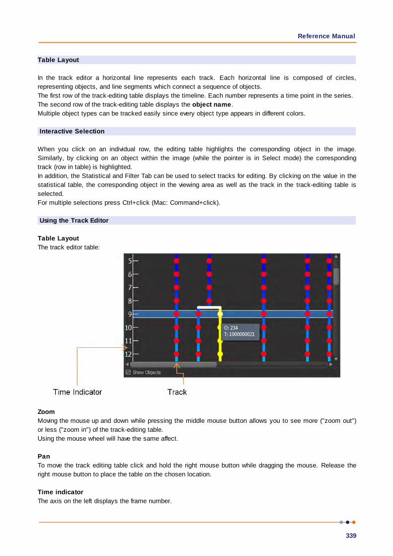
Reference Manual

339

Table Layout

In the track editor a horizontal line represents each track. Each horizontal line is composed of circles,

representing objects, and line segments which connect a sequence of objects.

The first row of the track-editing table displays the timeline. Each number represents a time point in the series.

The second row of the track-editing table displays the object name.

Multiple object types can be tracked easily since every object type appears in different colors.

Interactive Selection

When you click on an individual row, the editing table highlights the corresponding object in the image.

Similarly, by clicking on an object within the image (while the pointer is in Select mode) the corresponding

track (row in table) is highlighted.

In addition, the Statistical and Filter Tab can be used to select tracks for editing. By clicking on the value in the

statistical table, the corresponding object in the viewing area as well as the track in the track-editing table is

selected.

For multiple selections press Ctrl+click (Mac: Command+click).

Using the Track Editor

Table Layout

The track editor table:

Zoom

Moving the mouse up and down while pressing the middle mouse button allows you to see more ("zoom out")

or less ("zoom in") of the track-editing table.

Using the mouse wheel will have the same affect.

Pan

To move the track editing table click and hold the right mouse button while dragging the mouse. Release the

right mouse button to place the table on the chosen location.

Time indicator

The axis on the left displays the frame number.

IMARIS

340

Track

Each track is displayed in a vertical format by default. If connected components or Lineage algorithms are used

there may be a number of branch points. The branch points indicate where objects fuse or fragment, e.g. cells

undergoing division.

Object

Each data-point is displayed as an object in the track with a unique Object ID. The object will retain its unique

ID number- even if, for example, it is connected manually to another track.

If the mouse pointer is on an object, a tooltip appears that identifies the Object ID number (O) and track ID

number (T). You can untick the Show Objects checkbox to hide objects from the display.

Show Objects

Use this option to select to show or hide each object in the tracks from being visible.

Camera icon

Use the camera icon to save an image of the currently displayed tracks (either .tif or .svg formats) to a specified

location. The image will automatically open in the default graphics applicatin after saving is complete.

Mouse Selects

This option allows you to select objects or tracks as follows:

Object

Click Object to select an individual object, or number of specific objects. To connect two unconnected objects,

simply select both objects and click the Connect button. To disconnect two connected objects, select both

objects and click the Disconnect button.

Segment

Click Segment to select a specific segment (between branch points).

Branch

Select Branch to select the segment and the branched segments and objects that appear later in time only.

Pivot

Pivot enables selection of a segment and all segments and objects that are linked afterwards. This includes

objects later in time, and also backwards in time.

For example, selecting branch (left) selects only the connected segments and objects that are later in time.

Selecting Pivot (right) all connected segments and objects to be selected.

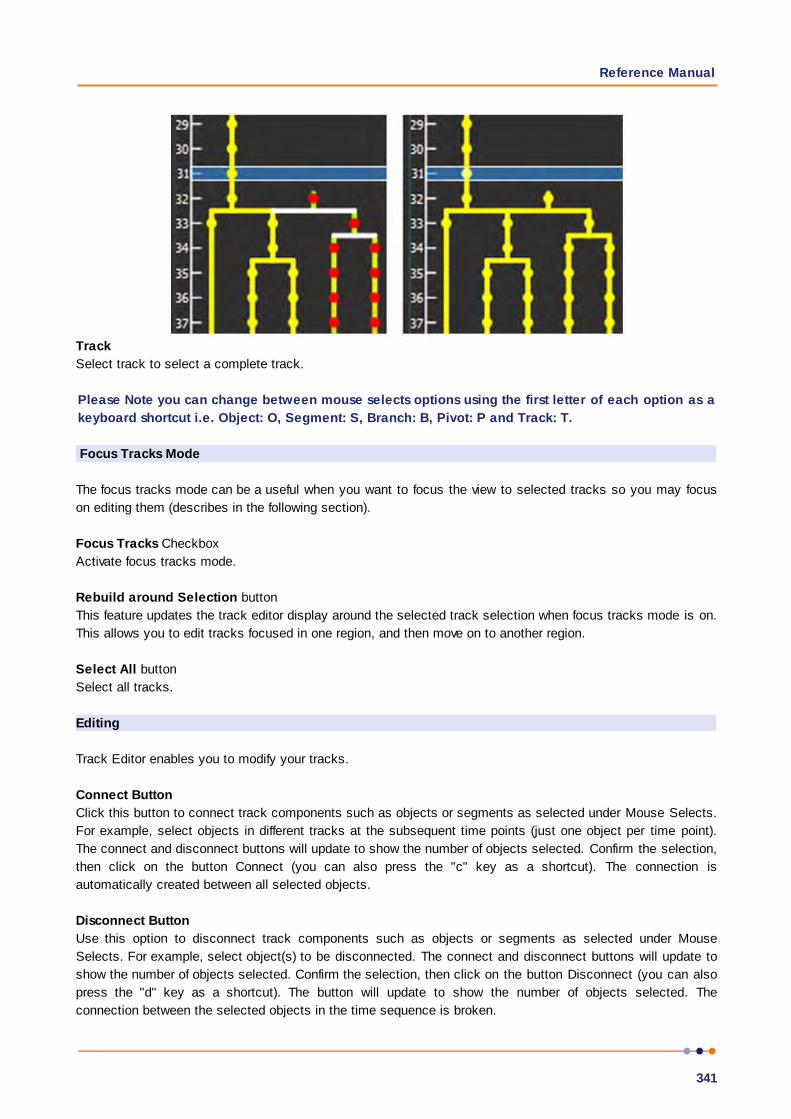
Reference Manual

341

Track

Select track to select a complete track.

Please Note you can change between mouse selects options using the first letter of each option as a

keyboard shortcut i.e. Object: O, Segment: S, Branch: B, Pivot: P and Track: T.

Focus Tracks Mode

The focus tracks mode can be a useful when you want to focus the view to selected tracks so you may focus

on editing them (describes in the following section).

Focus Tracks Checkbox

Activate focus tracks mode.

Rebuild around Selection button

This feature updates the track editor display around the selected track selection when focus tracks mode is on.

This allows you to edit tracks focused in one region, and then move on to another region.

Select All button

Select all tracks.

Editing

Track Editor enables you to modify your tracks.

Connect Button

Click this button to connect track components such as objects or segments as selected under Mouse Selects.

For example, select objects in different tracks at the subsequent time points (just one object per time point).

The connect and disconnect buttons will update to show the number of objects selected. Confirm the selection,

then click on the button Connect (you can also press the "c" key as a shortcut). The connection is

automatically created between all selected objects.

Disconnect Button

Use this option to disconnect track components such as objects or segments as selected under Mouse

Selects. For example, select object(s) to be disconnected. The connect and disconnect buttons will update to

show the number of objects selected. Confirm the selection, then click on the button Disconnect (you can also

press the "d" key as a shortcut). The button will update to show the number of objects selected. The

connection between the selected objects in the time sequence is broken.

IMARIS

342

< Button

Click this button to move a selected track left. When axis is inverted (horizontal) the selected track moves up.

> Button

Click this button to move a selected track right. When axis is inverted (horizontal) the selected track moves

down.

<< Button

Click this button to move a selected track all the way to the left. When axis is inverted (horizontal) the selected

track moves to the top.

>> Button

Click this button to move a selected track all the way to the right. When axis is inverted (horizontal) the

selected track moves to the bottom.

Flip

The Flip button may be used (with Pivot mode selected) to flip the order that the connected branched segments

and objects are displayed in about the pivot point.

Reorganize

The Reorganize button can be used after editing of tracks is complete so that tracks are displayed in a clear

and logical format without affecting the track arrangement during the editing process.

Invert Axis

Click the Invert Axis button to switch between displaying the tracks vertically (default) and horizontally.

Correct Drift

Refer to Drift Correction.

Algorithms

The Drift Correction is calculated based on the two algorithms, translational drift and translational and rotational

drift.

Translation

Upon translation, the object position is transformed to a straight line of identical orientation. Within the same

time point the relative distance of the objects is preserved.

Translation and rotation

Upon translation and rotation, the object position is transformed based on the image polar coordinates. Within

the same time point the relative distance of the objects is preserved.

Reference Manual

343

Please note: The number of the selected tracks affects the algorithm calculation.

Selection of a single track gives a complete description of a translation.

Selection of two tracks gives a minimum description of a translation and rotation algorithm (planar rotation).

A better fit between the time points is achieved when three or more tracks are selected.

Result DataSet size

After completion of the drift correction, the algorithm uses the final position of the initial and resulting image to

create a final image. The new image coordinates are calculated in accordance with the size of the original and

new image.

Select the Result data set option to determine which new image part will be displayed.

Crop largest common region

The final image will be the size of the common overlap between the original and the drift corrected image. Areas

of the image that have been shifted outside these boundaries (to allow alignment) will be cropped from the final

result.

New size equal to current size

The final image will be the same size as the original image. Areas of the image that have been shifted outside

these boundaries (to allow alignment) will be cropped from the final result.

Include entire result

The final image will be the size of the combined area of the original and corrected image.

Selecting the appropriate Result data set size may speed up the data visualization. This is especially important

with (with large data sets.)

Correct Cells positions

Activate this parameter and the Cells are automatically re-positioned after the drift correction. If this option is

not activated only the image volume is aligned.



11.1.6 Tab Filter

Please note: Before using you have to add a filter to the list (see below: button Add)!




criteria.









IMARIS

344


Filters

Add Button

To add a new filter, click on the button Add and choose one of the Filter Types from the drop-down menu.

Select the filtering type to be used in order to classify objects and specify the measurement of the criteria to be

used. The new filter appears in the list.

Delete Button


Filter Type


Filter category

A Category identifies, gathers and summaries a set of statistical values or calculations of a particular Object

Type.






.

These buttons allow you to choose the Category and determine the list of displayed statistical values. Clicking




selects the Category and removes the selected statistical variables from the list (turns the category button into

a light gray color).





active threshold.


circle again.



adjustment.





Reference Manual

345






Lower Threshold

Automatic


Manual


in the value or click the histogram to move the colored line and then a reduced/enlarged set of objects are

visualized.

Higher Threshold

Automatic


Manual


in the value or click the histogram to move the colored line and then a reduced/enlarged set of objects are

visualized.

Histogram



Manual. By clicking the histogram you move the colored line and the reduced/enlarged set of objects. To



to increase the threshold and to decrease the threshold move the line to the left. These changes are instantly


The numerical range of the statistics value (e.g. Quality) and the number and percentage of objects that fall into

the particular filtering class are displayed at the bottom of the threshold histogram.




Duplicate Selection to New Surfaces Button

Click on this button and all selected objects are copied to a new Surpass Group. The new group displays in the

Surpass Tree.

11.1.7 Tab Statistics

Cells statistics are automatically computed. For the statistical values please refer to the Section Menu Edit -

Preferences... - Statistics - Cells. The Statistics tab collects and displays the image's statistical values in

Imaris. The Statistics tab enables us to understand and compare different data sets through summarized

statistical values and graphical data presentations.

Several types of statistical tools enable convenient organization and analysis of heterogeneous statistical data.

IMARIS

346

The Statistics View is configured as follows:

a) Overall b) Detailedc) SelectionIn the statistical data set the first column contains the name of the variable, followed by columns with

calculated statistical data. Corresponding statistical variable values are presented in rows.

To sort the columns click on the arrow in column heading. Click again to reverse the sort order.

Overall Tab

Output of the Overall statistics provides an overview of the image's single determining variables. Only statistics

that are not measured on a per-object basis are displayed here.

Category


Type.



In Imaris there are the following Filter Categories: Surface , Surface Tracks , Spots , Spots Tracks ,



.






light gray color).


Detailed Tab

Tables in the Detailed Tab are showing a statistical data collected from all of the objects within the image. Apull down list offers the following types of Detailed statistical calculations: Specific Values

Average Values

Time Plots

The values displayed are always for the current time point. Selecting a variable that changes over time creates

a plot of selected values as a time function. The statistical variable value is plotted on the vertical axis and the

time is plotted on the horizontal axis. The current time point is indicated with a black vertical line. Each time

value is displayed as a point. Click inside the plot and move the time line. Moving the line changes the time

point. Altering the time point changes the variable value and the image.

Multiple value selection, available by Ctrl+ click, will plot a superimposed second selected value over the first

one.

Interactive two-way Selection

A click on an individual row of the table highlights the corresponding object in the image. Similarly, by clicking

on an element in the image (while the pointer is in Select mode) the corresponding row in table will be

highlighted. A possibility of multiple selections is available by pressing Ctrl+click (Mac: Command+click).

Reference Manual

347

Specific Values

In the Specific Values, a second pull down list at the top of the window displays available specific statistical

values. Select the variable and a list of values will be displayed.

Object Statistical Annotation option is available for Specific values parameters.

Average values

The Average table contains values determined on the basis of all values within a set of the selected variable.

Columns are labeled as follows:

Min (Minimum)- the smallest value within a set of values of the selected variable

Max (Maximum)- the largest value within a set of values of the selected variable

Mean – value of the sum of all values divided by number of values within a set

Std Dev (Standard deviation)- a measure of the values distribution around the mean values

Median- the middle value of the sorted set of variables

Sum- the sum of all values within a variable set

Count- number of values within a set

Unit- variable unit

Level/Distance

The black line on the time plot indicates where the mean value lies, the red indicates the median, the light

gray area shows the range between the min and max values and dark gray region labels the standard

deviation range with error bars.

Statistical variable classification:

1. Statistical variables associated with objects (Cells, Nucleus, Vesicles -volume, area, intensity values,

position, speed, displacement) have values at every time point. Therefore for these variables the Average values

are displayed per time point. Changing the time points, statistical variable values and images are consequently

changed.

2. Statistical values with data associated with Tracks (track duration, track volume mean, track displacement

length, track intensity) are not time dependent.

All values

If the option All values is selected for the detailed tab, all values will be displayed. Even though this option is

always readily available, it is discouraged to use it in order to avoid data clutter.


Selection Tab

Statistical tables for a selected object will be displayed. Change to the pointer mode Select and click on an

image element that has been detected/segmented. A possibility of multiple selections is available by Ctrl+click

(Mac: Command-click).

A pull down list offers two types of statistical calculations from a Selection:

Specific Values

Average Values

Time Plots






IMARIS

348


one.





Specific values




Average values

The Average table contains values determined on the basis of all the values within a set of the selected

variables for the selected image element(s). For further explanation see Average values Detailed statistics. This

choice only makes sense in the context of the Selection Tab if you have selected more than one element from

the image.





Buttons Overview

PC: Mac:

Select Cells Left-click Click

Select multiple Cells Ctrl + left-click Command + click

Buttons at the bottom of the Statistics tab

Button Settings -Configure a List of visible statistics values. Click on the button Settings and you switch to the window Preferences - Statistics - Cells.

Button Search - Search by object ID.

Type in the object ID in the data field. Click on the button Search.

Highlights the object in the viewing areaHighlights the object on the Detailed TabDisplays of the values on the Selection Tab

Button Cells - Duplicate Selection to new Cells.

Click on this button and all selected elements are copied to a new Cell. The new Cell appears in the Surpass

Tree, and the old one is hidden, but still available.

Button Statistical Annotation

Click this button and an object statistical annotation will be automatically generated in the viewing area. This

option is available only when Specific is selected

Button Export - Export Statistics on Tab Display to File.

Reference Manual

349

Only the statistics that are shown within the current tab will be exported.

Button Export - Export selected Data for plotting

Exports the selected statistical value for plotting. The selected value has to be time dependent.

With a click on the button Export the Export Statistics window opens. Select the file type (Comma Separated

Values *.csv, Excel file *.xls, or Excel XML *.xlm). If you select MS Excel as file type, the program starts

automatically.

Button Export - Export All Statistics to File.

All of the statistics (that are enabled in the statistics settings) will be exported for Overall and Detailed tab data.

When the Selection tab is selected, pressing the Export all Statistics to File button, will export All the

statistics (that are enabled in the statistics settings) of all the selected objects, not all the statistics of all the

objects.



automatically and the sheets show up one after another (this will take several seconds).

See also:

Menu Edit - Preferences... - Statistics - Cells

11.1.7.1 Statistical AnnotationsStatistical annotations provides the opportunity to view and annotate image objects with the statistical data

values. Using this function, the individual objects in an image are labeled with the specified statistical values

and the statistical data is displayed directly in the viewing area

Imaris objects can be labeled with a set of any number of the user-defined statistical values.

The Statistical Annotation button provides a convenient interface to label the object with the statistical data.

Click this button and an object statistical annotation will be automatically generated in the viewing area. The

selected object is annotated for all time points with the specified statistical values.

How to add Statistical Annotation

In the Statistical tab choose the Detailed or Selection Tab.

In the viewing area select the object or group of objects. Change to the pointer mode Select and click on an

image object that has been detected/segmented. For multiple selections press Ctrl+click (Mac: Command-

click)

In the Detailed or Selection Tab a pull down list offers Specific Values or Average Values as types of

statistical parameters.

Select the statistical value associated with the particular object type you are working with.

Press the Statistical Annotation button .

In the viewing area the object label appears showing selected statistical values as a statistical annotation.

The statistical annotation shows by default the name of the selected statistical parameter and its value.

The color white displays the text of annotations associated with statistical values.

For a single object, all selected statistical parameters are placed in the same annotation box. Once the object

is labeled, selecting the additional statistical parameter updates the object statistical annotation; the new

parameter and its value is added in the viewing area.

If the image is a time series, the statistical annotation will be visible in the viewing area for all time points.

Selecting a statistical variable that changes over time creates an statistical annotation that consequently

changes with every time point.

The statistical annotation displays values always for the current time point.

IMARIS

350

The Annotation options will allow you to modify and specify the contents and format of the object labels.

To modify and adjust the statistical label click on the Icon Annotation , press Ctrl + Shift + P, or in the menu

bar select File – Annotation.

11.1.8 Tab Color

Choice of the Object type is presented in a drop-down window. Select Cell, Cell Tracks, Nucleus, Nucleus

Tracks, Vesicle (multiple types) or Vesicle Tracks.

Depending on the chosen object type selection of the variables is listed.

The following color types are available:

Labels

Base

Statistics Coded

Time Mapped

Object ID

Track ID

11.1.8.1 Tab Color-LabelsThe labels associated with the data set is displayed as a list.

Click Only show labelled objects to show only data which have labels associated with them.

Note that if there is more than one label associated with an object, the object will be displayed as a combined

color. Non-labelled objects are displayed in the base color.

Transparency

Transparency defining amount of light allowed to pass through. Click this tool to change the percentage from

0% (complete opacity) to 100% (complete image transparency).

11.1.8.2 Tab Color-BaseRGB

The RGB color model is an additive color model in which Red, Green and Blue color information are combined

together to reproduce the required color. The color values may be changed either by clicking on the color wheel

to select a color or by direct numeric entry for the Red, Blue or Green component (values range from 0 to 1).

Light reflection

Quality of the object material is further characterized by reflection properties.



applied to the object. Default setting has no specular intensity.

Emission- light emitted from the material defines the self-illumination. Default setting emits no light.

Transparency

Transparency- defines the amount of light allowed to pass through an object. Click this tool to change the


Reference Manual

351

Palette


In the Palette, colors are labeled and grouped together. The scrolling window contains the 14 color combination




button. After being added, these color choices are stored and can be used with other Imaris objects.

11.1.8.3 Tab Color-Statistics CodedDepending on the chosen object type the Statistical variable selection is listed in the drop-down window. For

example, if Cell/Nuclei/Vesicle is chosen as the Object type, available Statistical data will be the Cell/Nuclei/

Vesicle linked variable. Similarly, variables for Tracks will be listed, if the object type is selected to be Tracks.

Statistics Colorbar Properties

Statistics colorbar are displayed in the viewing area. The upper one is the colorbar range for Cel/Nucleus/

Vesicles and the lower one is the colorbar for the Tracks.

Show Colorbar

Check the box to see the statistics colorbar in the viewing area.

Show Title

Check this box to see the title in the statistics colorbar.

Show Range

Check this box to see the range in the statistics colorbar.

Font color in colorbar is adjustable by selecting a color within the color map.

Colormap

Button Reset

Click the Reset button to set the image back to the original values.

Colormap




Colormap range

Colormap range-specify the limits for the colorbar.

Min - lower color limit

Max - upper color limit

Button Auto

Click the button Auto and the system detects the real min and max values and sets the Max. and Min. limits

automatically to these values.

IMARIS

352

Transparency



11.1.8.4 Tab Color-Time MappedThis option is only available when Tracks (see above) is selected as an Object Type. The color range for the

Tracks goes from blue to white to the range of time points.

Transparency



11.1.8.5 Tab Color-Object IDObject ID assigns a random color to every object. This is available for all surpass components. For Cells, this is

the default coloring.

11.1.8.6 Tab Color-Track IDTrack ID assigns a fixed, random color to each object. This mode is useful for validating tracks as an object will

have the same color through the track duration. Erroneous behavior can easily be detected and corrected using

the Edit Tracks functions. Refer to the Tab Edit Tracks section.

Transparency



11.2 Clipping PlaneThe Clipping Plane cuts away objects on one side of the plane. It can be freely moved and rotated in the scene

and allows you to look inside any object. The Clipping Plane consists of a colored frame with a white double rod

in the middle.

To change the position and orientation of the Clapping Plane in the View Area the Pointer must be in Select

mode.

How to Add a new Clipping Plane?

Select menu 3D View - Clipping Plane.

The Surpass Tree list is automatically updated and in the Clipping Plane - Properties the Settings parameter

are displayed. The Clipping Plane is displayed in the viewing area.

To clip another object, this object must be placed behind the clipping plane within the Surpass Tree. It must be

in the same group as the Clipping Plane and it must be placed below the Clipping Plane.

Change Position of Clipping Plane

The position of the Clipping Plane can be changed. Choose the pointer mode Select, highlight the Clipping

Plane in the viewing area and click on the bigger diameter rod. It will turn colored as it is selected, move it to

set the Clipping Plane to the required position.

Reference Manual

353

Rotate Clipping Plane around Axes

The Clipping Plane can be rotated around the x-, y-, and the z-axes. In Select mode click the smaller diameter

rod. It will turn colored as it is selected, move it to rotate the Clipping Plane.

See also:

Surpass View - Overview - Surpass Tree

Surpass View - Overview - Camera Toolbar - Pointer (Mode Select)

11.2.1 Tab Settings

Position

Button Recenter

The Clipping Plane center is moved to the data set center.

Orientation

Button YZ Plane

Button XZ Plane

Button XY Plane

The Clipping Plane is oriented parallel to either the yz-plane, the xz-plane or the xy-plane.

Button Flip

Click on the Flip button to flip the orientation of the clipping plane.

Configuration

Button Store

Button Recall

After changing the position and/or orientation of the Clipping Plane, the new configuration can be stored by

clicking on the Store button. The position previously stored can be recalled by selecting the Recall button.

Camera

Button Orthogonal View

The camera is set to a position which is perpendicular to the Clipping Plane.

Show Frame

To make the frame visible, check this box.

Perpendicular Movement

The pointer must be in the pointer mode Select. Place the mouse within the image. To change the orientation of

the rod press the Ctrl button. The Clipping Plane is moved in the directions parallel to the plane.

See also:

Surpass View - Overview - Camera Toolbar - Pointer (Mode Select)

IMARIS

354


Clipping Plane Mouse & Keyboard Functions

Left-click on plane & drag Move plane to desired position

Left-click on the bigger diameter rod & drag Move plane to desired position

Left-click on the smaller diameter rod & drag Rotate plane to desired position

See also:



Clipping Plane Mouse & Keyboard Functions

Click on plane & drag Move plane to desired position

Click on the bigger diameter rod & drag Move plane to desired position

Click on the smaller diameter rod & drag Rotate plane to desired position

See also:


11.3 External ObjectSurpass provides the ability to import External objects (both, non-Imaris and Imaris objects) and display them

concurrently with a Surpass object for comparison.

Only the External objects with the extensions *.iv (Inventor file) or with extensions *.vrml (VRML2 files) or .wrl

(WRL files) can be imported.

The imported External objects can be rotated, scaled and translated.

For example, previously calculated Surfaces, which have been exported as Inventor files, can be imported to

another data set.

How to Add a new External Object?

Select menu 3D View - External Object.

The Surpass Tree list is automatically updated and in the External object - Properties the Settings parameter

are displayed.

See also:

Menu 3D View - Export Selected Objects ...

11.3.1 Tab Settings

The object properties area displays a number of parameters for the positioning and display of the External

object. The following display/handling options can be checked:

Box Handle

The object shows a surrounding box with handles. These handles allow you to transform/distort the object in

the x-, y-, and z-direction.

Reference Manual

355

Trackball

The object shows surrounding circular lines. These lines allow rotation of the External object in any direction.

File Path Field

Display of the file path (to load the object, see below).

Button Load...

To select and load a data set as a External object click on the button Load... and the Load External Object

File window is displayed. Select the file to be loaded as External object. The External object will be only loaded

if the selected files have the extension *.iv (Inventor file), *.vrml (VRML2 files) or .wrl (WRL files). Click on

the button Open.

Button Reset Size and Location

Clicking this button sets the External object back to its original size and position before any translational,

scaling or rotational operations have been performed.

Fix Ratio

If this option is checked and if scaling is performed on the External object by entering a value, the same scaling

factor is applied to all three dimensions.

Position/Scaling

The following positional/scaling options are available:

Translation

Use these fields to move the External object in the x-, y-, or z-direction.

Rotation

Use this field to rotate the External object around the x-, y-, or z-axis.

Scaling

Use this field to scale the External object in one of the dimensions (or all together if Fix Ratio, see above, is

checked). Fix Ratio is only valid with this method of scaling.

11.3.2 Tab Color

Color Tab edit, manage and assign material colors of an Object.

RGB



color or by direct numeric entry for the Red, Blue or Green component (values range from 0 to 1).

Light reflection

The quality of the object material is further characterized by reflection properties.



applied to the object. Default setting is for no specular intensity.

Emission- light emitted from the material defines the self-illumination. Default setting is for no emission of

IMARIS

356

light.

Transparency



Palette








External Object Mouse & Keyboard Functions

Left-click white box & drag Scale object from center

Left-click white box + Ctrl & drag Scale object from opposite corner

Left-click trackball & drag Rotate object

Shift + left-click trackball & drag Set up a rotation axis

See also:



External Object Mouse & Keyboard Functions

Click white box & drag Scale object from center

Click white box + Ctrl & drag Scale object from opposite corner

Click trackball & drag Rotate object

Shift + click trackball & drag Set up a rotation axis

See also:


11.4 FilamentIn Imaris dendritic trees are represented by a set of vertices and edges. The Vertex is drawn as a node or a

dot and defines the center axis of the dendrites. An edge is presented as a line connecting two vertices. The

entity of vertices and edges is referred to as filament graph.

Parts of the filament graph can be classified as spines either collectively, based on some statistical values, or

individually by the user, by determined specifications.

Starting, ending and branching vertices are classified into dendrite beginning point, dendrite branch

point, dendrite terminal point, spine attachment point, spine branch point, and spine terminal point

depending on their position in the graph (refer to the following image).

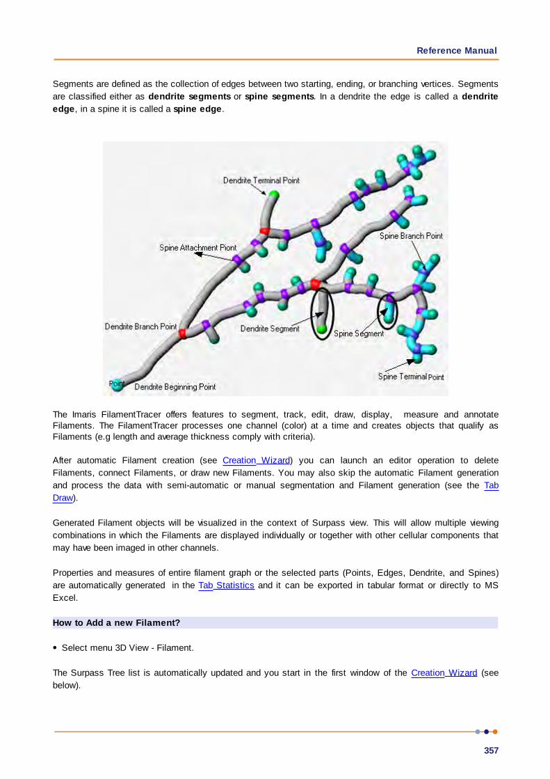
Reference Manual

357

Segments are defined as the collection of edges between two starting, ending, or branching vertices. Segments

are classified either as dendrite segments or spine segments. In a dendrite the edge is called a dendrite

edge, in a spine it is called a spine edge.

The Imaris FilamentTracer offers features to segment, track, edit, draw, display, measure and annotateFilaments. The FilamentTracer processes one channel (color) at a time and creates objects that qualify asFilaments (e.g length and average thickness comply with criteria).

After automatic Filament creation (see Creation Wizard) you can launch an editor operation to delete

Filaments, connect Filaments, or draw new Filaments. You may also skip the automatic Filament generation

and process the data with semi-automatic or manual segmentation and Filament generation (see the Tab

Draw).

Generated Filament objects will be visualized in the context of Surpass view. This will allow multiple viewing

combinations in which the Filaments are displayed individually or together with other cellular components that

may have been imaged in other channels.

Properties and measures of entire filament graph or the selected parts (Points, Edges, Dendrite, and Spines)

are automatically generated in the Tab Statistics and it can be exported in tabular format or directly to MS

Excel.

How to Add a new Filament?

Select menu 3D View - Filament.

The Surpass Tree list is automatically updated and you start in the first window of the Creation Wizard (see

below).

IMARIS

358

See also:


3D View - Filament - Creation Wizard (for automatic Filament creation)

3D View - Filament - Tab Draw (for interactive Filament tracing method)

For information on statistics calculations used refer to Filament

11.4.1 Data Input

The FilamentTracer is designed to operate on 3D time-resolved images. These images can be multi-channel

(multiple colors) but only one channel will be traced at a time. The following input images are acceptable:

The ideal input is a fluorescently labeled confocal image. Such images generally have good contrast (due to

selective labeling) and good resolution in all three spatial dimensions.

3D images can also be acquired using a standard microscope (non-confocal) equipped with a CCD camera

and a stepper motor. Non-confocal optical arrangements do not provide resolution along the optical axis

which is why every single plane consists of in-focus components and out-of-focus components. These

images require deconvolution prior to tracing. The technique of deconvolution uses information about the

imaging process (the point spread function) to remove the out-of-focus components from every section.

Finally there are 3D images taken in transmission light microscopy. Staining is usually less specific than for

fluorescence techniques and it will therefore be more difficult to automatically segment the Filament.

Deconvolution can also be applied to transmission images although - theoretically - its performance is weaker

than for fluorescence methods.


The automatic filament graph compilation (creation) is guided by a wizard-like user interface and consists

essentially of five steps.

Select the appropriate algorithm (or quit the automatic filament creation and draw the filaments interactively).

Define a Region of Interest

Select source channel and do some pre-processing.

Segmentation to specify filamentous and non filamentous parts.

Graph compilation and finishing.

The Creation Wizard allows you to move forward or backwards until the optimal parameters are found.



In the first window of the Filament Creation Wizard, you find the algorithm settings. Here, you have to decide, if

you want to load a set of previously stored creation parameters or to create a new one.


Parameters option.

See also:

3D View - Filament - Creation Wizard - Algorithm

3D View - Filament - Creation Wizard - Preprocessing

3D View - Filament - Tab Draw (for interactive filament tracing method)

Reference Manual

359

11.4.2.1 AlgorithmIn this first window of the Creation Wizard you decide, if you want to go for an fully automated filament creation

using one of the two predefined algorithms (AutoPath-no loops or Threshold-loops, see below); or if you want to

draw the filaments interactively.

Note: If you do not want to use the automatic filament creation wizard select the Skip automatic creation,

edit manually button.


Terminates the creation wizard and activates the interactive filament tracing method.





Then you can choose to segment a Region of Interest (ROI) only, to create Tracks after the objects detection

or to Skip automatic creation.



image segmentation.






Select Algorithm

The automatic filament creation provides two algorithms to choose from:

AutoPath (no loops)

Threshold (loops)

AutoPath (no loops)

The automated AutoPath Algorithm:

Produces a tree-like filament

Is based on local intensity contrast

Connects large start- and small end-points

If you select this algorithm please refer to Section: 3D View - Filament - Creation Wizard - Autopath Algorithm

(no loops)

Threshold (loops)

The Threshold based Algorithm:

Produces a filament with loops

Is based on an absolute intensity threshold

Thinning to a skeleton

IMARIS

360

If you select this algorithm please refer to Section 3D View - Filament - Creation Wizard - Threshold Algorithm

(loops)

Calculate Diameter of Filament from Image

Check this box and the Filament diameter is calculated based on the image data.

Uncheck the box and the Filament diameter will taper smoothly from the starting point to the end points.

Segment a Region of Interest-ROI



Track (over time)

Check this box if you want to track Filament over time, for details please refer to the tab Tracking.

Filament Wizard Buttons

Button Next

Press Next to proceed with the next of the Creation Wizard.

Button Finish

Press Finish and based on the selected algorithm (see above) Imaris runs through all parameters (coming on

the following windows of the Creation Wizard) using the default settings. At the end of the calculation the

Filaments are displayed in the viewing area.

Button Cancel

Click on this button if you do not want to use the automatic graph compilation. Use instead the interactivefilament tracing method. The parameters on the tab Settings are displayed in the properties area. Please referto Section 3D View - Filament - Tab Draw to adjust the parameters.

11.4.2.2 Autopath Algorithm (no loops)The Autopath (no loops) algorithm consists of the following steps:

Region of Interest

Dendrite Points Diameter

Classify Dendrite Points

Dendrite Diameter

Spine Points Diameter

Classify Spine Points

Spine Diameter

Tracking

Finish

11.4.2.3 ROIHere you define the region of interest (ROI). Parameters such as width, height and location of the ROI are used


X, Y, Z, Time

Min, Max, Size

Reference Manual

361

Minimum, maximum and Size of ROI coordinate values, can be specified either by entering the value in the

value fields or changing the values by clicking on up-and down arrows at the right hand side of the value fields.

Alternatively the location and size of the ROI can be adjusted directly in the viewing area.

Size of the ROI:







Memory Usage:


Regions of Interest



Button Add



Button Delete


Total Memory Usage:



Button Back


Button Next


Button Finish

Click on Finish to calculate the desired Filament and display the Filament in the viewing area.

Button Cancel

If you do not want to create Filament automatically click on Cancel.

11.4.2.4 Dendrite Points DiameterSelect Source Channel

Select the respective source channel, from which the Dendrite structure is to be created.

Starting Points

Detect a new starting point -a new starting point of the filament will be determined, based on the value given

IMARIS

362

for the largest diameter.

(largest Diameter: e.g. Dendrite Beginning)

Enter a value of the maximum (largest) diameter of dendrite to specify the Starting point diameter.

Seed Points

(Thinnest Diameter e.g. Dendrite Ending)

Enter a value of the minimum (smallest) diameter of dendrite to specify the Seed points diameter.

Rebuild Options

As part of the rebuilding process in step three of the Creation wizard – Dendrite Points Diameter, a new option

exists for selecting a Starting Point.

Use Existing Dendrite

Use Existing Dendrite- the previously determined dendrite points will be used in the creation of new starting

point. Therefore, in the next creation step (Starting point threshold) an option for Manual Start point editing in

(shift+right click) will not be available.


Button Back


Button Next


Button Finish

Press Finish and Imaris runs through all parameters (coming on the following windows of the Creation Wizard)

using the default settings. At the end of the calculation the Filaments are displayed in the viewing area.

Button Cancel

Click on this button if you do not want to use the automatic graph compilation. Use instead the interactivefilament tracing method. The parameters on the tab Settings are displayed in the properties area. Switch to thetab Draw and please refer to Section 3D View - Filament - Tab Draw to adjust the parameters.

By re-entering the Creation Wizard, either after selecting Rebuilding Algorithm or for Processing additional

ROI(s) a new option exists for selecting a Starting Point.

See also:

3D View - Filament - Tab Settings

3D View - Filament - Tab Draw (for interactive filament tracing method)

11.4.2.5 Classify Dendrite PointsThresholds are used to classify the detected dendrite’s starting points and seed points.

The detected dendrite starting point(s) are visualized in the image by different colors. The respective histograms

are displayed.

The threshold can be set manually or automatically.

Reference Manual

363




active threshold.


circle again.



adjustment.
















considered.






Starting Points Threshold

Display of the starting points threshold and the respective histogram. The threshold can be adjusted by entering

a new value in the data field or by moving the colored threshold line (click & drag) in the histogram. The updated

points are visualized in the viewing area.

Manual Starting Points addition/deletion in Creation Wizard

Manual addition of starting points in the filament structure is available by pressing Shift+ right-click. Shift+ right-

click on an existing filament start point (created either automatically or manually added) and the selected

starting point will be deleted.

IMARIS

364

Seed Points Threshold

Display of the end points threshold and the respective histogram. The threshold can be adjusted by entering a

new value in the data field or by moving the colored threshold line (click & drag) in the histogram. The updated

points will be visualized in the viewing area.

Manual Seed Points Addition/Deletion in Creation Wizard

Manual Addition of Seed points in the filament structure is available by Shift+ left-click. Shift+ left-click on an

existing point, (created either automatically or manually added) and the selected point will be deleted.

Remove Seed Points Around Starting Point(s)

Check the box and all seed points located within the radius of the sphere centred at the starting point are

removed. The boundary of the sphere is defined by the value Diameter of Sphere Region(s).

Diameter of Sphere Region(s)

Enter the diameter of the sphere centred at the beginning point. Default value set to twofold of the starting

points diameter.

Remove Disconnected Segments

These parameters allow the user to adjust and improve the accuracy of the interactive filament tracing. This

feature will help eliminate misdirected filament branching due to labeling that is not continuous, contains low

signal regions, and for images that contain high levels of noise.

By selecting the Remove Disconnected Segments, it enables the algorithm to continue filament tracing for a

distance defined in the Max Gap Length field.

This parameter determines which branches are identified as disconnected based on gap length and excludes

them from the filament.

When this option is enabled, you first set parameters to generate threshold mask using smoothing and/or

background subtraction. These smoothing and/or background subtraction parameters are identical to those

used in Surface rendering.

A connection between disconnected branches will be created only when the maximum spacing between two

disconnected masks does not exceed the defined length in the Max Gap Length field.

Smooth With

Set Smooth With value as you would define the parameter for a surfaces object. This define the Guassian filter

width used when background subtraction is enabled.

The value is either automatically calculated from the voxel sizes or it can be directly entered into the numerical

field.



background value is then subtracted from every voxel in the image; Baseline Subtraction is performed.

Max Gap Length

The distance in which the objects connection is automatically established is based on the value defined in the

Max Gap Length value.

The Max Gap Length defines the maximum distance, which is allowed to be missing in order to create a

Reference Manual

365

connection between two disconnected segments. If the distance is longer than the defined gap distance, then

the segments will not be considered part of the filament.


Button Back


Button Next


Button Finish


Button Cancel

If you do not want to create a Filament automatically click on Cancel.

11.4.2.6 Dendrite DiameterThe option is only available if in the step Algorithm the Calculate Diameter form the image is selected.

The threshold value is based on the local contrast and the respective histogram is displayed.

The defined threshold value is used for the dendrite diameter calculation.




active threshold.


circle again.



adjustment.










The effect of changing the threshold value is directly visible in the viewing area.




IMARIS

366

Algorithm

The Algorithm provides two methods to calculate dendrite diameter.

The method of diameter calculation has no effect on the position of the filament centre axis, located at the local

intensity peak (yellow disk)

For cases where the centre axis is closer to the centre of diameter mask (blue hatched area), the difference

between the options is smaller.

Shortest Distance from distance map

The Shortest Distance from Distance Map option considers the radius as the shortest distance from the seed

point (yellow disk) to the edge of the filament mask (blue line), in any (x,y,z) direction

This method is typically less sensitive to diameter overestimation due to axial (z) blur. It is recommended when

the centre axis is overall well centred on the structure and the real structure has a roughly circular cross-

section.

Approximate Circle of cross section area

The Approximate Circle of cross section Area option is recommended when the centre axis position is not well

centred in a large diameter structure e.g large irregular spine heads. The area of the green circle is equal to the

cross-section area determined in the threshold step.

Reference Manual

367


Button Back


Button Next


Button Finish


Button Cancel


11.4.2.7 Spine Points DiameterSpine

Detect Spines

Check this box to Optimize the Creation wizard for Spine Detection; creating the highly branched filament

structure.

Uncheck the box Detect Spines and the Spine channel selection and the Seed Points diameter are disabled.

Spines detection and creation are not performed in the following creation procedure.

Select Source Channel

Select the respective source channel, from which the spines are to be computed. The default channel is the

same as for the dendrite detection.

Seed Points

(Thinnest Diameter e.g. Small Spine Head)

Enter a value of the minimum (smallest) diameter of spine head to specify the Seed points diameter.

IMARIS

368

Maximum Length

The Maximum Length is estimated spine length, the length from the dendrite center to the furthest Spine seed

point.

Allow Branch Spines

Check the Allow Branch Spines option to allow formation of the spines's bifurcation points. To form bifurcation

point the two spine's vertices have to be in the vicinity of 1 voxel.


Button Back


Button Next


Button Finish


Button Cancel


11.4.2.8 Classify Spine PointsThe option is only available if in the step Spine Points Diameter the Detect Spine option is selected.

Spine

Seed Points Threshold

Thresholds are used to classify the spines seed points. The detected Spine seed points are visualized in the

image. The respective histogram is displayed.

The threshold can be set manually or automatically.




active threshold.


circle again.



adjustment.





Reference Manual

369






The threshold can be adjusted by entering a new value in the data field or by moving the colored threshold line

(click & drag) in the histogram. The updated points are visualized in the viewing area.






Button Back


Button Next


Button Finish


Button Cancel


11.4.2.9 Spine DiameterThe option is only available if in the step Spine Points Diameter the Detect Spine option is selected.

The threshold value is based on the local contrast and the respective histogram is displayed.

The defined threshold value is used for the Spine diameter calculation.




active threshold.


circle again.


IMARIS

370


adjustment.











Algorithm

The Algorithm provides two methods to calculate Spine diameter.

Shortest Distance From Distance Map

The Spine diameter is calculated as the shortest distance between spine center point and spine surface.

Approximate Circle of Cross Section Area

The diameter of the approximate circle of cross-sectional area is determined as a value of the spine diameter.


Button Back


Button Next


Button Finish


Button Cancel


11.4.2.10 TrackingThe filament object consists of a set of the dendrites, the spine points and the connection between them.

Tracking allows objects to be traced throughout sequential frames of time data set. Each object maintains an

unique identity in the output measurements.

This tab only appears, if the Track (over Time) is checked (Algorithm Settings).

The Filament tracking tab provides Autoregressive Motion algorithms, which model the filament movement.

The algorithm utilizes the object’s direction and speed information from one single time point to predict the best

potential object position at the next time point.

Based on the tracking of the entire Filament graph, the algorithm predicts the future positions of the Dendrite

Beginning Point, Branching and Terminal Points as well as the Spine Attachments, Spine Terminal Points

Reference Manual

371

Based on these predicted positions, the best matches to the candidate points can be determined. The

algorithms use a Linear Assignment algorithm and a Total Cost function to find the best track connections. The

total cost computation is based on the change in distance.


This algorithm models the motion of the filament graph’s center of gravity as an autoregressive AR1 process.

The AR1 model looks back to one time-point, and predicts that the object will move again the same distance

and in the same direction. The user-specified Maximum Distance value is the distance in which the object is

allowed to deviate from the predicted position. Some changes in direction are tolerated because of the value of

the maximum distance parameter, and because the AR1 algorithm performs correlations only to one previous

time-point.

Track Filaments Center of Gravity

Max Distance





It can happen that the object segmentation fails for some time points, which can break a Track apart into two

Tracks. The gap-closing algorithm tries to continue the movement of a disappearing object and connects the

Tracks if they reappear.

Close Gap

Select this option and the gap-closing algorithm will be implemented.

Max Gap Size






The Max Gap Size defines the maximum number of the consecutive time points which are allowed to be


Track Dendrites

Select this option and the Dendrite points will be tracked.

When the Track Dendrite option is not selected the drop-down list remains inactive.

From the drop-down list you can select the type of Dendrite points to be tracked. There are two options:

Dendrite Branch Points

Dendrite Terminal Points

Please note: The tracking of the Dendrite Beginning point is automatically computed based on the

tracking of the entire Filament structure.

Enable

IMARIS

372

Check the box to enable the selected Dendrite points to be traced

Max Distance





It can happen that the object segmentation fails for some time points, which can break a Track apart into two

Tracks. The gap-closing algorithm tries to continue the movement of a disappearing object and connects the

Tracks if they reappear.

Close Gap


Max Gap Size








Please note: The spine tracking options are only available if the spines have been previously

created.

Track Spines

Select this option and the Spine points will be tracked.

From the drop-down list select the type of Spine points to be tracked. There are three options:

Spine Attachment Points

Spine Branch Points

Spine Terminal Points

Enable track

Check the box to enable the selected Spine points to be traced.

Close Gap


Max Gap Size




Reference Manual

373





Please note: The spine tracking options are only available if the spines have been previously

created.


Button Back


Button Finish


Button Cancel


11.4.2.11 Finish ROI ProcessingThe selected parameters will be used to complete the computation of a Filament structure in an image. By

selecting one of six finishing options a Filament structure will be created in the following ways:

1. Additional Regions - re-enters creation process (in step two-ROI) and uses the same set of parameters for

a new ROI to create the filament structure.This option is only available if you work with a time data set. When

the data set contains multiple time points, the Filament Creation Wizard can create Filament objects for all

time points with the same set of parameters.

2. Entire Image in All Time Points- the entire image is processed with the same parameters used for the ROI

processing and the filament structure is created for the entire image and all time points. Only available if you

work with a time data set. When the data set contains multiple time points, the Filament Creation Wizard can

create Filament objects for each time point with the same set of parameters.

3. All Done- creates a filament structure only within an ROI.

Please refer to Tab Rebuild. In step three of the Creation wizard – Point Diameter an option exists for selecting

a Starting Point (Use existing filament or Detect a new starting point).

Note: The Use Existing Filament option requires that the new ROI overlaps with some portion of the

existing filament.


Button Back


Button Next


Button Finish

IMARIS

374


Button Cancel


11.4.2.12 Threshold Algorithm (loops)The threshold (loops) algorithm consists of the following steps:

Preprocessing

Segmentation

Graph Compilation

Finish

11.4.2.13 PreprocessingSource Channel

Select the respective source channel, from which the Filament structure is to be computed.

Feature Preprocessing

Enable Feature Preprocessing

Check the box and the following parameters are adjustable. Uncheck the box and the following parameters are

grayed. Preprocessing is not necessary if the data is already deconvolved or if the noise has already been

removed by a Gaussian filter. The preprocessing will be applied to the source channel and the result will be

added as new Filament Working channel in the Display Adjustments.

Appr. Filament Diameter

An approximate minimal Filament diameter has to be provided.

Preserve Edges

You can also enable an edge preserving preprocessing to maintain filamentous structures when the Threshold

(loops) algorithm is selected. It is not available if the Autopath (no loops algorithm is selected.

Before continuing you can inspect the result of the previous step with any viewer of Imaris: Slice, Section,

Gallery, Easy3D, Surfaces etc.


Button Back


Button Next


Button Finish

Press Finish and Imaris runs through all parameters (coming on the following windows of the Creation Wizard)

using the default settings. At the end of the calculation the Filaments are displayed in the viewing area.

Button Cancel

Click on this button if you do not want to use the automatic graph compilation. Use instead the interactivefilament tracing method. The parameters on the tab Settings are displayed in the properties area. Switch to thetab Draw and please refer to Section 3D View - Filament - Tab Draw to adjust the parameters.

Reference Manual

375

See also:


Menu Image Processing - Thresholding - Connective Baseline

3D View - Filament - Tab Draw (for interactive filament tracing method).

11.4.2.14 SegmentationSegmentation

Fill Cavities (fully enclosed volumes)

Check this box to avoid hollow regions. These regions would be enclosed by a Filament mesh, which is not

desired in most cases.

Note: Fill Cavities option is not available in Imaris version 7.7 onwards.

Connective Baseline

Type in two values for the lower threshold (colored line) and upper threshold (red line). You can also click into

the histogram. Left mouse button for lower, right mouse button for upper threshold or you can click & drag the

respective line.

Simple thresholding methods classify voxels purely based on a single intensity value. This approach often does

not lead to good results because the staining, the illumination, and the detection operate within a precise

range. The connective thresholding scheme takes care of this and searches for object voxels using an intensity

range rather than a single intensity.

You must provide two threshold values. The lower threshold (colored line) is the intensity below which a voxel is

recognized as part of the background, the upper threshold (red line) is the minimal intensity for a voxel to be

part of the Filament object. Voxels with an intensity value between the two thresholds are treated as part of the

Filament object if and only if they are connected to a voxel within intensity above the upper threshold ("double

thresholding" with "feature-AND").

The result of the segmentation process described above is a clean image where the non-zero voxels are

describing the objects (Filaments and some non-filamentous structures). Because such a description of the

data is not suitable for morphometric analysis the structures are converted. Graph compilation is a process

involving several image processing operations such as skeletonization, erosion, dilation and the creation of a

vector definition for the Filaments. The result of the process is a database (kept in memory) describing the

Filaments as a set of segments that may contain branches.


Button Back


Button Next


Button Finish


Button Cancel

If you do not want to create a Filament click on Cancel.

IMARIS

376

See also:

Menu Image Processing - Thresholding - Connective Baseline

11.4.2.15 Graph CompilationGraph compilation

Minimal Ratio of Branch Length to Trunk Radius

Enter a minimal ratio of branch length to trunk radius (see figure below). Branches shorter than this value will be

removed.

R B

Ratio of branch length (B) to trunk radius (R).

Find Dendrite Beginning Point

A dendrite beginning point has to be specified for specific statistic values (e.g. tree order). The point is selected

from the trunk position with the biggest radius.


Button Back


Button Next


Button Finish


Button Cancel

If you do not want to create a Filament click on Cancel.

11.4.2.16 FinishFinish

To validate the automatically generated graph and the prior segmentation, you can inspect the result together

with numerous Surpass modules: Ortho Slicer, Volume, Surfaces etc. You can optionally superimpose the

segments with the original slices of the image stack using Imaris OrthoSlicers. OrthoSlicers are planes, which

are perpendicular to any of the three spatial axes and extend throughout the entire image volume.

Reference Manual

377

Build Filaments for all Time Points

Only available if you work with a time data set. When the data set contains multiple time points, the Filament

Creation Wizard can create Filament objects for each time point with the same set of parameters. They will be

visible within the Surpass Tree. However the 3D Filament graph is only visible according to its time point.

Delete Working Channel

The Filament Working channel can be kept for another use. Principally it is not needed any more when finishing

the Filament graph.


Button Back


Button Next

This button is grayed in the last window of the Creation Wizard.

Button Finish


Button Cancel

If you do not want to create Filaments click on Cancel.

11.4.3 Filament Properties

When the creation process is finished, the Tab Rebuild disappears while some other property Tabs appear.

They allow the manipulation of the filament graph:

Tab Rebuild

Only appears when you Add a new Filament.

Tab Settings

Change Filament appearance and inspect selection statistics.

Tab Rebuild

Re-enter the creation process.

Tab Draw

Manually draw filaments and connections.

Tab Edit

Select automatically filament parts and delete or smooth them.

Tab Statistics

Inspect all statistic values.

Tab Color

Change the color appearance (material) of the filament.

See also:

3D View - Filament (Add a new Filament)

3D View - Filament - Tab Settings

IMARIS

378

3D View - Filament - Tab Rebuild

3D View - Filament - Tab Draw

3D View - Filament - Tab Edit

3D View - Filament - Tab Statistics

3D View - Filament - Tab Color

11.4.4 Tab Settings

On the tab Settings you can edit and adjust the display options.

Select the Filament option to adjust quality and style of the filament graph.

Select the Filament Tracks option and you can edit and adjust settings that determine the display of

connections between the Track filament graphs.

Select the Point Tracks option and you can edit and adjust settings that determine the display of connections

between the dendrite beginning, branch and terminal points, as well as spine attachment, branch and

terminal points of the filament graphs.

11.4.4.1 FilamentStyle

Line

Cylinder

Cone

The visualization of the graph is done as lines with a specified thickness (pixel), as cylinders (with a defined

diameter), or cones (using the measured graph diameter).

Show Dendrites

Check the box in the heading to highlight dendrite points in the filament. The key points are highlighted with

color-coded spheres.

Beginning Point

Check this box to highlight the dendrite beginning points.

Branch Points

Check this box to highlight the dendrite branch points.

Terminal Points

Check this box to highlight the dendrite terminal points.

Show Spines

Check the box in the heading to highlight spine points in the filament. The key points are highlighted with color-

coded spheres.

Attachment Points

Check this box to highlight the spine attachment points.

Branch Points

Check this box to highlight the spine branch points.

Reference Manual

379

Terminal Points

Check this box to highlight the spine terminal points.

Render Quality

With the slider you can adjust the render quality of the filament. Moving the slider to the left reduces the render

quality, moving it to the right increases render quality.

11.4.4.2 Filament TrackTracks Style/Quality

The box Style/Quality has settings that determine the display of connections between the Track objects.

Cylinder

This option displays the tracks connections drawn as cylinders.

Line

This option displays the tracks connections drawn as lines.

Off


Width

Diameter

Depending on the previous selection you adjust the width of the line or diameter of the cylinder.

Render Quality

When you select Cylinder (see above) the Render Quality is adjustable using the slider.

Filament Tracks

Displacement

Check the box Displacement to show the displacement of a Track as an arrow. To assign another color click on

the Color symbol to open the Color Editor.

Radius Scale

Edit field for the displacement vector radius.

Color Editor

Select a desired color for the displacement arrow.

Dragon Tail


are shown depending on the selected time points.

Slider

Adjust the number of time points using the slider.

IMARIS

380

11.4.4.3 Point TracksTracks Style/Quality


Cylinder

This option displays the tracks connections drawn as cylinders.

Line


Off


Width

Diameter


Render Quality


Filament Tracks

Displacement



Radius Scale


Color Editor


Dragon Tail



Slider


11.4.5 Tab Rebuild

Rebuild

Imaris stores the list of operations and the mapping of parameters.

Click on drop-down window and six choices are available for re-entering the Filament Creation Wizard.

Rebuild All

Rebuild Dendrite

Rebuild Dendrite Diameter

Rebuild Spine

Rebuild Spine Diameter

Reference Manual

381

Rebuild Tracks

Select the rebuild algorithm to be applied from the list. As you select the rebuild algorithm, the creation wizard

opens at the appropriate step.

The wizard retains all the prior parameters allowing you either to reuse or edit them while re-creating the

filament structure.

If you choose the rebuild option, the window Rebuild Diameter opens which performs the diameter calculationfor either the Rebuild Dendrite Diameter or the Rebuild Spine Diameter.

Rebuild Diameter

Select the Specific Source channel, from which the Dendrite/Spine structure is to be computed. To specify thechannel, enter the channel number in the field.

The Creation Wizard is using previous parameter settings as initial values. You can easily change

just a few parameters without going in detail through all the parameters.

Spine Rebuilding

The spines can be created at any later time by re-entering the creation wizard, since the spine detection and

creation is the default last step of the Filament Creation Wizard.

Note that spine rebuilding options are available if spines were not previously created.

Keep Data

The option Keep Data should be selected depending on whether the existing Filament graph should be

discarded, or re-used in the Filament rebuild process.

If this option is selected, the previously created filament structure is kept. The Wizard creates a newly added

filament that is merged with the existing one.

If this option is not selected, the previously created filament structure is discarded and the Wizard creates a

new filament structure.

All Time Points

The option All Time Points should be selected depending on whether the parameters used for creating the

Filament structure should be applied to the selected time point only or to all time points.

If this option is selected, the same set of creation parameters used for selected time point is reused to the

create filament structure for all time points.

If the option is not selected, the creation parameters are used only for the selected time point.

All Time Point is an option available only with time resolved data sets.

In the rebuild process the following structure of the filament creation is applied:

1. According to the setting of the Keep Data option the existing Filament structure is discarded or re-used

2. The selected Rebuild algorithm is completed

3. In the case of the time resolved data sets, according to the setting of All Time Points options, the

parameters are either used to create the filament structure for the selected time point only or to create the

filament structure for all time points.

IMARIS

382

Button Rebuild ObjectsClick on this button to start the rebuild.

Creation Parameters

The Creation Wizard saves parameters and processing instructions so the Filament computation can be

repeated for the same region, a different region, or the entire image. The Creation Parameters values are listed

as a table.

In step three of the Creation wizard – Dendrite Points Diameter, a new option exists for selecting a Starting

Point.

Use existing filament

Detect a new starting point

Use existing filament- the previously determined starting point will be used in the new filament structure.

Therefore, in the next creation step (Starting point threshold) an option for Manual Start point editing in (shift

+right click) will not be available.

Detect a new starting point -a new starting point of the filament will be determined, based on the value given

for the largest diameter.





There are two options to store your creation parameters

Arena


Arena








under the Edit/Preference/Creation Parameters. This option allows you to use the creation parameters in future

on another data set. These saved parameters can then be imported and re-used on any new data set should

you wish to perform an identical analysis sequence. This option is also useful for sharing the parameters with

other users to allow them to perform the same analysis on their own data sets.

Within the Surpass view storing allows the parameters to be reused or modified. In addition, this option is useful


it.


Reference Manual

383





Click on the Store Parameters for the Batch button to open the Store Creation Parameter window.



11.4.6 Tab Draw

Method

When it is not possible to use Imaris automatic filament creation algorithms, either semi-automatic or manual

creation will allow you to create filament objects by manually marking the object location in using method

AutoPath, AutoDepth or Manual.

AutoPath

The AutoPath function automatically computes all the paths from a user-defined starting point to the end of the

structure. If you select AutoPath the button Set Starting Point is available. If you select this method please

refer to Section AutoPath (3D View - Filament - Draw - AutoPath).

AutoNetwork

The Auto Network is an additional option that is disabled by default, but it can be enabled in Advanced

Preferences by setting the Preference SurfaceAppFilament/EnableAutoNetwork to true. The AutoNetwork

function automatically detects and creates all connections according to a user-defined diameter value. The

results of the Auto Network function are visualized as lines. From the created network, the user can decide

which part of the structure will be connected.

To set the starting point press Shift + right-click on the preferred location of the structure.

Place the mouse at the ends of the structure and the path is displayed.

To draw the displayed path press Shift + left click.

Please note: To create "way-points" press Shift+left-click at the location of the waypoint, and simultaneously

press Shift-right-click (at the same location) in order to move forward toward the real end-point.

Network


Select the respective source channel, from which the Network structure is to be created.

Diameter

Enter a value of the minimum (smallest) diameter to be detected.

Create Network Button

Click on this button to start the Network structure creation.

Show Network

Select this box to visualize the created network connections.

IMARIS

384

AutoDepth

The AutoDepth function adds the automatic computation of the depth while doing manual segmentation (e.g. if

the manual segmentation is done while looking at xy-plane, z-coordinate will be automatically computed). If you

select this method please refer to Section AutoDepth (3D View - Filament - Draw - AutoDepth).

Manual

The manual segmentation feature is used to edit automatically traced Filaments or to build the Filaments

manually from the image template. If you select this method please refer to Section Manual (3D View -

Filament - Draw - Manual).

Setting

Diameter

Set the Diameter for the cursor. The size of the cursor determines the resolution at which the tracing is

calculated (larger cursor provides lower resolution but is a faster calculation and less precision- but often these

low resolution paths are effective).

Type

Select between Dendrite and spine options


Select the source channel you will use to draw the filament.

Button Set Selection as Starting Point(s)

If you select as Method AutoPath (see above, selection of the drawing Method) the button Set Selection as

Starting Point(s) is available.

Select a point and click on this button to define the starting point of the filament.

Correction

AutoCenter

This option runs an automatic centering when the path is added (after pressing shift+left-click).

AutoDiameter

Select this option to run an automatic diameter calculation when the path is added (after pressing shift+left-

click). The calculation takes the mouse cursor size on shift+left-click as an input parameter (initial guess of

diameter). The mouse cursor size should roughly correspond to the diameter of the filament for the calculation

to succeed.

View

Select between the two viewing options:

Torch View

Provides a highlighted area to help allow you to focus on an area of interest. The size of the area illuminated by

the torch can be adjusted using the mouse wheel.

Reference Manual

385

Full View

Provides a normal view through the full image area.

Both Torch and Full View options are described and compared in the AutoPath and AutoDepth sections along

with the Depth Visibility controls.

Slice

If you select the Method as Manual, see above (and also the section Manual) for further information the Slice

parameter settings are available.

YZ Plane

XZ Plane

XY Plane

Select the plane orientation of the drawing board: yz, xz, xy.

Automatic Placement

When this parameter is activated, the position is set automatically to the location of the highest data intensity.

In order to avoid unwanted horizontal or vertical drawing offsets, the camera is set to a perpendicular position

with an orthogonal projection. In this case the camera can only zoom or pan but not rotate.

x ... um

Display of the Slice the position.

Slider

The position of the drawing board can be altered in perpendicular direction by the Slice slider. The same is

achieved using the Arrow-keys of the keyboard (Arrow up, Arrow down).



See also:Menu Edit - Show Display Adjustment

3D View - Overview - Camera Toolbar - Pointer3D View - Filament - Draw - AutoPath3D View - Filament - Draw - AutoDepth3D View - Filament - Draw - Manual

11.4.6.1 AutoPathThe AutoPath function automatically computes all the paths from a user-defined starting point to the end of the

structure. If you select AutoPath the button Set Starting Point is available.

Use the Channel drop-down options to specify the channel on which the calculation runs.

Placing a new start point cancels the previous calculation and starts again from the new start point.

When a start point is placed close to an end point the path will automatically connect.

The most recently drawn filament is automatically highlighted.

Press Shift+T to switch between Torch View and Full View modes.

Pressing Ctrl+8 is useful immediately after adding a path to turn on InMotion for validation of the tracing.

Autopath mode respects clipping planes: It chooses the start and end points only within the visible part of the

volume. (Note that the clipping plane frames and handles may be turned off so they do not selected by

mistake when making other adjustments to the image).

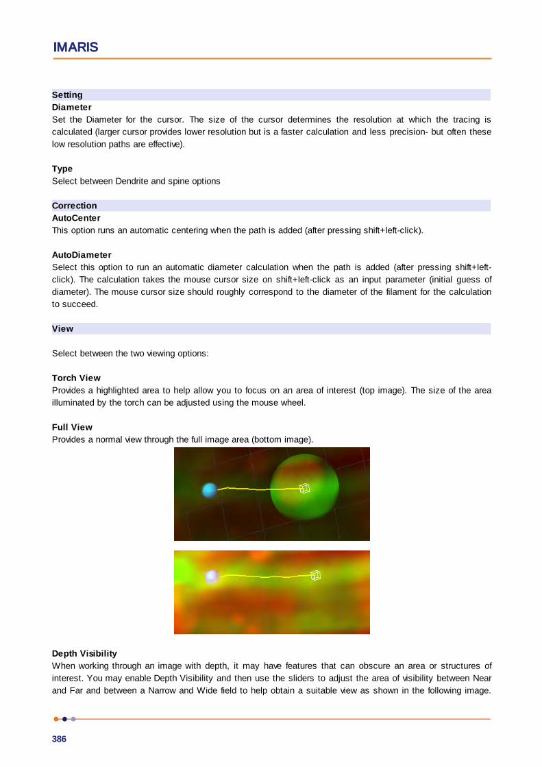
IMARIS

386

Setting

Diameter




Type

Select between Dendrite and spine options

Correction

AutoCenter


AutoDiameter




to succeed.

View


Torch View

Provides a highlighted area to help allow you to focus on an area of interest (top image). The size of the area

illuminated by the torch can be adjusted using the mouse wheel.

Full View

Provides a normal view through the full image area (bottom image).

Depth Visibility

When working through an image with depth, it may have features that can obscure an area or structures of

interest. You may enable Depth Visibility and then use the sliders to adjust the area of visibility between Near

and Far and between a Narrow and Wide field to help obtain a suitable view as shown in the following image.

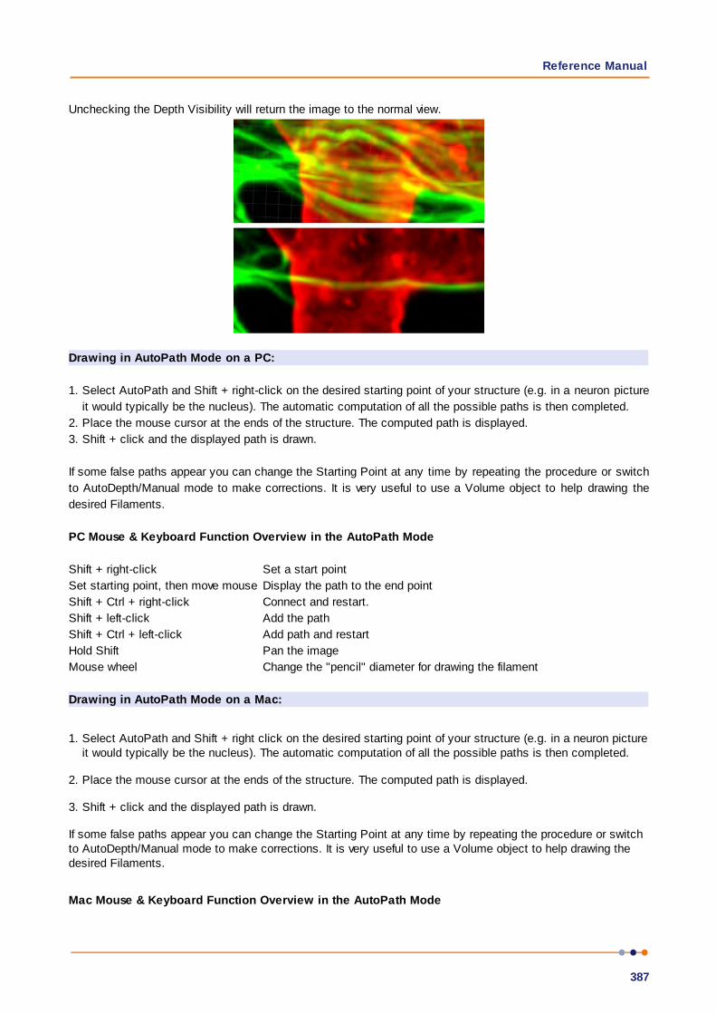
Reference Manual

387

Unchecking the Depth Visibility will return the image to the normal view.

Drawing in AutoPath Mode on a PC:

1. Select AutoPath and Shift + right-click on the desired starting point of your structure (e.g. in a neuron picture

it would typically be the nucleus). The automatic computation of all the possible paths is then completed.

2. Place the mouse cursor at the ends of the structure. The computed path is displayed.

3. Shift + click and the displayed path is drawn.

If some false paths appear you can change the Starting Point at any time by repeating the procedure or switch

to AutoDepth/Manual mode to make corrections. It is very useful to use a Volume object to help drawing the

desired Filaments.

PC Mouse & Keyboard Function Overview in the AutoPath Mode

Shift + right-click Set a start point

Set starting point, then move mouse Display the path to the end point

Shift + Ctrl + right-click Connect and restart.

Shift + left-click Add the path

Shift + Ctrl + left-click Add path and restart

Hold Shift Pan the image

Mouse wheel Change the "pencil" diameter for drawing the filament

Drawing in AutoPath Mode on a Mac:

1. Select AutoPath and Shift + right click on the desired starting point of your structure (e.g. in a neuron pictureit would typically be the nucleus). The automatic computation of all the possible paths is then completed.

2. Place the mouse cursor at the ends of the structure. The computed path is displayed.

3. Shift + click and the displayed path is drawn.

If some false paths appear you can change the Starting Point at any time by repeating the procedure or switchto AutoDepth/Manual mode to make corrections. It is very useful to use a Volume object to help drawing thedesired Filaments.

Mac Mouse & Keyboard Function Overview in the AutoPath Mode

IMARIS

388


Set starting point, then move mouse Display the path to the end point

Shift + Command + right-click Connect and restart.

Shift + left-click Add the path

Shift + Command + left-click Add path and restart





Notes

There is no visual indication of the progress of the autopath calculation. One way to find this out iindirectly is by

moving the mouse pointer to different positions in the image. For those positions where the calculation has

already arrived a tracing will be shown. For those positions where the calculation has not yet arrived no tracing

is shown.

Since it is very easy to trace a small piece and then continue the tracing from there users can work without

interrupt.

11.4.6.2 AutoDepthThe AutoDepth function adds the automatic computation of the depth while doing manual segmentation (e.g. if

the manual segmentation is done while looking at xy-plane, z-coordinate will be automatically computed).

An autosnap feature enables easy drawing along the filament structure as you do not need to click in the

exact centre. When ambiguities arise, autodepth keeps track of multiple paths until the ambiguities resolve.

(Only the best path is displayed to the user).

Press Shift+T to switch between Torch View and Full View modes.

Pressing Ctrl+8 is useful immediately after adding a path to turn on InMotion for validation of the tracing.

Autodepth mode respects clipping planes: It chooses start and end points only within the visible part of the

volume. (Note that the clipping plane frames and handles may be turned off so they do not selected by

mistake when making other adjustments to the image).

Setting

Diameter




Type

Select between Dendrite and Spine options

Correction

AutoCenter


AutoDiameter




to succeed.

Reference Manual

389

View


Torch View

Provides a highlighted area to help allow you to focus on an area of interest (top image). The size of the area

illuminated by the torch can be adjusted using the mouse wheel.

Full View

Provides a normal view through the full image area (bottom image).

Depth Visibility

When working through an image with depth, it may have features that can obscure an area or structures of

interest. You may enable Depth Visibility and then use the sliders to adjust the area of visibility between Near

and Far and between a Narrow and Wide field to help obtain a suitable view as shown in the following image.

Unchecking the Depth Visibility will return the image to the normal view.

Drawing in AutoDepth Mode on a PC:

Select AutoDepth, press the Shift-key and hold down the left mouse button to draw a Filament. The depth is

automatically computed by comparing local intensities.

IMARIS

390

Drawing in AutoDepth mode is then similar to drawing in Manual mode. In order to fully use the potential of the

AutoDepth mode, the pictures should not be too noisy. If this is the case, pre-filtering would be then necessary.

PC Mouse & Keyboard Function Overview in the AutoDepth Mode

Shift + left-click & drag Draw a filament into the volume



Drawing in AutoDepth Mode on a Mac:

Select AutoDepth, press the Shift-key and hold down the mouse button to draw a Filament. The depth is

automatically computed by comparing local intensities.

Drawing in AutoDepth mode is then similar to drawing in Manual mode. In order to fully use the potential of the

AutoDepth mode, the pictures should not be too noisy. If this is the case, pre-filtering would then be necessary.



Mac Mouse & Keyboard Function Overview in the AutoDepth Mode

Shift + click & drag Draw a filament into the volume



Notes

Pressing the d-key on the keybord while drawing enables an eraser so you can work backwards and redraw

from an earlier point. This works only on those parts of a filament that were drawn right before pressing the d-

key.

11.4.6.3 ManualThe manual segmentation feature is used to edit automatically traced Filaments or to build the Filaments

manually from the image template. Essentially you draw the Filaments onto the image, which serves as a

visual reference (template). Drawing is done in the xy-plane. For z-positioning in the image you can choose to

change planes manually (Arrow-keys or mouse) or to have the system change the planes automatically in such

a way that the center of the Filament is kept in focus.

An orthogonal section plane appears within the Surpass view. Use the channel visibility and the Display

Adjustments to optimize the viewing. In order to draw Filaments onto the drawing plane switch the mode for the

mouse pointer from Navigate to Select.

If you select Manual the Slice parameter settings are available.

Drawing in Manual Mode on a PC:

Select Manual in the Draw box and press the Shift-key and hold down the left mouse button to begin drawing.

The circle on the drawing plane indicates the Filament diameter.

The diameter can also be changed using the mouse wheel. To make a connection to an existing Filament, start

painting on this Filament. If the filamentous structure runs perpendicular to the drawing plane, use the right

Reference Manual

391

mouse button to alter the plane orientation.



PC Mouse & Keyboard Function Overview in the Manual Mode

Left-click plane & drag Change plane position perpendicular to its orientation

Shift + left-click Set a filament vertex

Shift + left-click plane & drag Draw a filament

Right-click plane Change the plane orientation (from XY to YZ to XZ)


PageUp Increase the "pencil" diameter for drawing the filament

PageDown Decrease the "pencil" diameter for drawing the filament

Num plus Increase the extended section (of the drawing plane)

Num minus Decrease the extended section (of the drawing plane)

Arrow up Change slice position up

Arrow down Change slice position down

X Set the plane orientation to YZ

Y Set the plane orientation to XZ

Z Set the plane orientation to XY

Drawing in Manual Mode on a Mac:

Select Manual in the Draw box and press the Shift-key and hold down the mouse button to begin drawing.

The circle on the drawing plane indicates the Filament diameter.

The diameter can also be changed using the mouse wheel. To make a connection to an existing Filament, start

painting on this Filament. If the filamentous structure runs perpendicular to the drawing plane, use the right

mouse button to alter the plane orientation.

Mac Mouse & Keyboard Function Overview in the Manual Mode

Click plane & drag Change plane position perpendicular to its orientation

Shift + click Set a filament vertex

Shift + click plane & drag Draw a filament

ctrl + click plane Change the plane orientation (from XY to YZ to XZ)


PageUp Increase the "pencil" diameter for drawing the filament

PageDown Decrease the "pencil" diameter for drawing the filament






IMARIS

392

11.4.7 Tab Edit

Up to this point in the analysis process, most steps have been carried out automatically. You have influenced

the tracking process by specifying a set of parameters. The Tab Edit allows you to make changes to the graph

topology and the number of nodes and segments in the filament graph. You make these changes directly by

processing part or all of the existing filament graph, or by operating on the 3D view of the graph.

Mouse Selection

Selecting a tool will change how the mouse interacts with the objects within the viewing area to match the

properties of that selection. Specify how to select parts of the Filament by a single mouse click on the Filament

graph.

Please Note: The selection of the filament type can be very different depending on which selection

is chosen in the Track Edit tab. The selection is governed by the selection mode under both the Edit

and Track Edit tab. The basis for the selection is the Mouse Selection mode found under in the Edit tab.

Expand selection on full Spines

Expand the initial selection set outwards from the original selected filament element until all attached spines

objects are included in the selection.

Point

Point selects the smallest part of the segmented filament graph, only the position nearest to the mouse

pointer.

Segment

Segment selects the graph section between two key vertices (branch points, beginning point, or ending points)

of the same class, ether dendrites or spines.

- Between the dendrite beginning point and dendrite branch point

- Between the dendrite branch points

- Between the dendrite branch point and dendrite terminal point

- Between the spine attachment point and spine terminal point

- Between the spine attachment point and spine branch point

- Between the spine branch point and spine terminal point

Branch

Branch selects the graph starting from the selected point to all the connected terminal points of the same class

(a beginning point should be defined first for this mode).

Between the Dendrite Attachment or Dendrite Branch point to the Dendrite Terminal point for Dendrites.

Between the Spine Attachment point or Spine Branching point to the Spine Terminal point for Spines.

Filament

The Filament option selects the entire Filament graph.

Select Parts from Filament

There are various methods to make automatic selections on the whole Filament graph.

Reference Manual

393

R B

Button Rel. Branch...

Rel. Branch selects short parts of the Filament defined by the ratio of the branch length to trunk radius B/R.

Button Loops...

Loops finds circular closed Filaments limited by a maximum length.

Button Invert

Invert selects all unselected parts of the graph and de-selects all selected parts.

Button Abs. Branch

Abs Branch selects all branches shorter than an absolute length B.

Button Path

Path requires at least two selected points from the Filament graph. The shortest path between these two points

will be selected.

Button Clear

Clear removes the selection.

Selection

The following buttons apply only to the previously selected parts (see above) of the Filament.

Button Assign as Dendrite

Click on this button to assign the selection as dendrite.

Button Assign as Spine

Click on this button to assign the selection as spine.

Button Assign as Dendrite Beginning Point

Click on this button to assign the selection as dendrite beginning point.

Button Smooth

Removes the roughness of the current selection. It affects the position and the diameter of all segments except

the branch points and end points.

Button Duplicate

Click on this button to create a duplicate of the current selection. The new Filament item appears in the

IMARIS

394

Surpass Tree.

Button Delete

Click on this button to remove the current selection.

Filaments

The following buttons apply to the entire Filament.

Clear Dendrite Beginning Point

Click on this button to remove the dendrite beginning point.

Button Smooth

Smooth removes roughness from the Filament path. It affects the position and the diameter of all segments

except the branch points and end points.

Button Split

Unconnected parts of the Filament can be split into separate Filament objects. The new objects will appear as

new Items in the Surpass Tree. This allows individual coloring and individual statistics.

Button Merge...

In Imaris it is possible to merge Filament objects into one Filament objects. This button is only available if you

have two or more Filament items in the Surpass Tree. Click on this button and the window Merge selected

Objects to "Filament X" displays.

Check the boxes in front of the desired Filaments or use the button Select All.

Button Clear All

Use this button to clear the Filaments selection.

Button OK

If you want to merge the Filaments click on OK.

Button Cancel

If you do not want to merge the Filaments click on Cancel.

Connect & Translate selected Edges (Vertices)

Check this box to connect and translate selected edges.

Button Export...

The whole Filament graph can be stored in the Neuron file format (*.hoc). The Neuron application is free and is

able to do electrical simulations.

Intensity-based

Source Channel

Select the respective source channel, from which the structure is to be created.

Diameter...

Enter a value for the the minimum (small) diameter to be detected. The maximum (large) diameter is set in

Imaris to be the small diameter x 10. The threshold value has a default value of 3.0- however this can be

Reference Manual

395

adjusted in Advanced Preferences. Under SurfaceAppFilament set the value of DiameterContrastThreshold from

3.000 to the required value.

Selection

Button Center

Click on this button to re-center the selection after e.g. adjusting the diameter, according to the image intensity

gradient.

Button Diameter

Click on this button to recalculate the filament diameter of the selection to the value set in the Diameter field.

Button Join

Select the objects to be joined in the image by Ctrl + left-click (Mac: Command+ left-click). The selected point

or segment will be highlighted, then click Join. A new filament structure will be created structurally joining

previously unconnected points or segments.




Mouse Selects




Object

Segment

Branch

Pivot

Track

Please Note: The selection of the filament type can be very different depending on which selection

is chosen in the Track Edit tab. Selection is governed by the selection mode under both the Edit and

Track Edit tab.

Note also you can change between mouse selects options using the first letter of each option as a


How to use the Selection Tools

Selection of different filament elements and tracks can be made within the Edit and Track Edit Tabs.

To make a suitable selection for time resolved filament images, you may need to make the object selection by

clicking on the Mouse Selection options both under the Edit and Track Edit tabs.

Once you have selected the Filament graph element under the Edit tab you can also use the selection options

under the Track Edit tab to decide whether the object to be selected is just for a single time point or for all

time points.

Under the Track Edit tab you can decide either to select objects for a single time point by choosing the

IMARIS

396

option Filament or for all time points along the selected track by selecting the option Track.

For example, if under the Edit tab the mouse pointer is the Segment option and under the Edit Track tab the

mouse selection is the Filament option, then the Segment will be selected for a single time point.

However, if you alter the selection under the Track Edit tab to the Track option, the particular Segment will be

selected for all time points along that track.

Table Layout










In addition, the Statistical Tab and Filter Tab can be used to select tracks for editing. By clicking on the value in

the statistical table, the corresponding object in the viewing area as well as the track in the track-editing table

is selected.


Visualization options

Zoom




Pan



Time indicator


The current time point is indicated by a vertical line highlighted with the current selection color.

To modify the time point, do one of the following:

1. Moving the slider in the Time bar modifies its position in time and changes the time point in the track editor.

2. Clicking on the time point within the track-editing table automatically moves the time line indicator to the

corresponding point.

Double-clicking the time indicator, fixes the position of the current time point at the center of the track-editing

table, regardless of the selected zoom or pan options)

Editing

Track Editor has several features that help you modify your tracks

Reference Manual

397

Connect Button






Disconnect Button






< Button


> Button


down.

<< Button



>> Button



Flip



Reorganize



Invert Axis


Correct Drift


IMARIS

398

Focus tracks mode may be useful when editing tracks- refer to the Cells Edit Track section.

Algorithms


drift.

Translation










Result DataSet size



new image.





result.








Correct Filaments positions

Activate this parameter and the filaments are automatically re-positioned after the drift correction. If this option

is not activated only the image volume is aligned.



Reference Manual

399

11.4.9 Tab Filter

Please note: Before using, you have to add a filter to the list (see below: button Add)!




criteria.










Filters

Add Button




Delete Button


Filter Type


Category


Type.






.




To remove the category from the list, re-click on the Category button. Re-clicking on the category button

deselects Category and removes the selected statistical variables from the list (turns the category button into a

light gray color).


IMARIS

400

Lower Threshold

Automatic


Manual



Higher Threshold

Automatic


Manual



Histogram



By clicking the histogram you move the colored line and a reduced/enlarged set of objects. To change the






Dendrite) is displayed at the bottom of the threshold histogram.




Duplicate Selection to New Filament Button


Surpass Tree.


Filament statistics are automatically computed. For the statistical values please refer to the Section Menu Edit

- Preferences... - Statistics - Filament. The Statistics tab collects and displays the image's statistical values in





a) Overall

b) Detailed

c) Selection

In the statistical data set the first column contains the name of the variable, followed by columns with


To sort the columns click on the arrow in column heading. Click again to reverse the sort.

Reference Manual

401

Overall Tab



Category


Type.






.






light gray color).


Detailed Tab

A pull down list offers the following types of Detailed statistical calculations:

Specific Values

Average Values

Time Plots







one.





Specific Values



Average values



IMARIS

402








Unit- variable unit

Level/Distance




Selection Tab




A pull down list offers two types of statistical calculations from a Selection:

Specific Values

Average Values

Time Plots







one.





Specific values



Average values




the image.




Reference Manual

403


Button Settings -Configure a List of visible statistics values.

Click on the button Settings and you switch to the window Preferences - Statistics - Filament.



Highlights the object in the viewing area

Highlights the object on the Detailed Tab

Displays of the values on the Selection Tab

Button Filament - Duplicate Selection to new Filament.

Click on this button and all selected elements are copied to a new Filament object. The new Filament appears

in the Surpass Tree, and the old one is hidden, but still available.



option is available only when Specific is selected







automatically.





objects.




See also:

Menu Edit - Preferences... - Statistics - Filament

11.4.11 Tab Color

In Tab Color you can edit, manage and assign colors material to the Filament object.

Object Type

The choice of Object type is presented in drop-down window Dendrite, Spine, Dendrite Beginning Point,

Dendrite Branch Point, Dendrite Special Branch Point (more than three segments attached to one point),

Dendrite Terminal Point, Spine Attachment Point, Spine Branch Point, and Spine Terminal Point.

IMARIS

404

Choose one of the objects from the drop-down list and depending on the chosen object type selection of the

variables is listed.

The following color types are available:

Labels (default)

Base

Statistics Coded

11.4.11.1 Color Type- LabelsThe labels associated with the data set are displayed as a list.

Click Only show labeled objects to show only data which have labels associated with them.


color. Non-labeled objects are displayed in the base color.

Transparency



11.4.11.2 Color Type-BaseRGB

The RGB color model is an additive color model in which Red, Green and Blue color information is combined

together to reproduce the required color. The color values may be changed either by clicking on the color wheel


Light reflection





Emission- light emitted from the material defines the self-illumination. The default setting is for no emission of

light.

Transparency



Palette







Reference Manual

405

11.4.11.3 Color Type-Track IDTrack ID assigns a fixed, random color to each object. This mode is useful for validating tracks as an object will



Transparency


0% (complete opacity) to 100% (complete image

11.4.11.4 Color Type-Statistics CodedStatistics Coded

Depending on the object type selection the Statistical variable selection is listed in the drop-down window. For

example, if Dendrite is chosen as the Object type, the available Statistical types will be the Dendrite linked

variables.


Statistics colorbar are displayed in the viewing area.

Show Colorbar


Show Title


Show Range



Colormap

Button Reset


Colormap




Colormap range

Colormap range-specify the limits for colorbar.



Button Auto

IMARIS

406

Click the button Auto to detect the system the real min and max values and sets the Max. and Min. limits


Transparency




Filament Mouse & Keyboard Functions on the Tab Draw

AutoPath Mode

Shift + right-click Set a starting point into volume. Multiple paths/branches can be drawn from this

start point.

Set starting point,

then move mouse

Display the path to the end point

Shift + left-click Draw the path visible on screen to the cursor. Does not change the start point or

calculation thread from the start point.

Shift + Control + Left Click Draw the path visible on screen to the cursor. Starts a new calculation from the end

of a drawn path. Continues on same filament path.

Shift + Control + Right

Click

Start a new calculation from an existing point on a drawn segment. This will create

a new branch point, if it is in the vicinity of a drawn segment.

Mouse wheel Change the filament diameter (to visualize change to Style Cone - Tab Settings)

AutoDepth Mode

Shift + left-click & drag Draw a filament into the volume


Manual Mode

Left-click plane & drag Change plane position perpendicular to its orientation

Shift + left-click Set a filament vertex

Shift + left-click plane &

drag

Draw a filament

Right-click plane Change the plane orientation (from XY to YZ to XZ)


PageUp Increase the filament diameter (to visualize change to Style Cone - Tab Settings)

PageDown Decrease the filament diameter (to visualize change to Style Cone - Tab Settings)








See also:


Reference Manual

407


Filament Mouse & Keyboard Functions on the Tab Draw

AutoPath Mode


Set starting point,

then move mouse

Display the path to the end point

Shift + left-click Draw the path visible on screen to the cursor. Does not change the start point or

calculation thread from the start point.

Shift + Command + Left Click Add the path.

Shift + Command + Right

Click

Connect and restart.



AutoDepth Mode

Shift + click & drag Draw a filament into the volume


Manual Mode

Click plane & drag Change plane position perpendicular to its orientation

Shift + click Set a filament vertex

Shift + click plane & drag Draw a filament

Command + click plane Change the plane orientation (from XY to YZ to XZ)


PageUp Increase the filament diameter (to visualize change to Style Cone - Tab Settings)

PageDown Decrease the filament diameter (to visualize change to Style Cone - Tab

Settings)






See also:


11.5 Reference FrameReference frames can be used for image alignment. When time series need to be rotated or shifted for better

alignment this transformation can be achieved using reference frames. Reference frames are orthogonal

coordinate systems that can be positioned manually. To facilitate reporting of Object Statistics in the reference

frame coordinate systems all positional and vectorial statistics values are automatically reported both in image

coordinates and in reference frame coordinates.

IMARIS

408

A time play mode lets you play through a movie so that reference frames stay still.

The Reference Frame Coordinate System

A reference coordinate system consisting of three orthogonal axes can be positioned anywhere within theimage and oriented in any direction by the user. The reference coordinate system can be positionedindependently for each time point. A user can for example, place a reference coordinate system so that oneaxis aligns with the anterior-posterior axis of a Zebrafish.

Reference frames are positioned manually by clicking into the 3D View.

To adjust orientation of the axes- Click on arrow of an axis and hold the left mouse button to adjust the orientation of the axes.

To move position of the axes- Click on the central sphere to translate/move the position of the axes within the image.

For a time series it is not necessary to place a reference frame at every time point. It is possible to position afew frames at a few time points and all frames in between will be interpolated.

It is possible to create multiple reference frames within one image.

Statistics Values reported in Reference Frame Coordinates

All statistical values of surpass objects (spots, surfaces, cells, filaments) are computed both in world

coordinates and in reference coordinates. In the Zebrafish example Imaris would report track-velocity vectors in

the reference coordinate system such that it is easy to filter for objects that move toward the head of the fish for

example.

Time Series with Fixed Reference Frame

When reference frames have been set for different time points of a time series it is possible to play the movie insuch a way that the reference frames stay still. This is depicted in the following sequence:

ImarisXT Interface

Reference Manual

409

Reference Frames can also be used and set through the ImarisXT interface.

Statistics Values

Reference frame specific statistics values for each surpass object are:

Distance from origin of reference frame.Velocity angles with axes of reference frame.

These statistics values allow you to color objects by their distance to a reference frame, or by their direction of

motion relative to the reference frame.

11.5.1 Settings Tab

Key Frame

Use the Previous and Next buttons to move between the key frames. The default option is interpolated

(displayed in the Key Frame Type field. To set a translational key frame enable the T option, or to set a

rotational key frame enable R option. Activating these options will update the description in the Key Frame

Type field.

Planes

Set the frame plane options between XY, XZ and YZ planes.

Tick the Visible checkbox to toggle the visibility of the Reference frame on or off.

Use the fix checkbox to fix the plane in position.

Set the extended section for each plane by using the up and down arrows to increase or decrease the value

incrementally through each plane, or enter the required value directly.

Interpolation mode

Select between No Interpolation and Linear Interpolation.

No Interpolation: the translational and rotational positions will remain fixed between each reference frame. They

may therefore appear to "jump" between reference frames.

Linear Interpolation the translation and rotation positions between reference frames will be calculated in linearly

interpolated increments. This will provide a smooth transition between reference frames.

Resample Image to align Reference Frames

Press this button to resample the image in the reference frame coordinates.

For information on drift correction please refer to the section Drift Correction.

11.6 Correct DriftIf there is object drift (e.g. a cell drift) during the image acquisition this can be corrected in Imaris using the

Correct Drift function.

Drift correction can be applied to images with multiple time points, or to tracked objects.

The result of the drift correction is either a translational and rotational correction of image time points or a

reference frame object.

IMARIS

410

Drift correction on an image

To apply drift correction to an image:

1. Load an image with multiple time points into Imaris.

2. Choose Image Processing / Image Alignment / Align Image, or Image Processing / Image Alignment / Set

Reference Frame.

Drift correction on an image is a parameter free method. It performs an automatic spots detection and tracking

on the image and then applies drift correction on these points. The spots are never visible in Imaris and there is

no way to adjust the spots detection. If this procedure does not produce adequate results, detect and track

objects using e.g. the Spots wizard and use the Correct Drift functionality on the Track Editor Tab of the

tracked objects.

Drift correction based on tracked objects

To perform drift correction based on tracked objects, load an image with multiple time points in Imaris, create

and track a surpass object, e.g. Spots. Switch to the Edit Tracks Tab and press the Correct Drift button. Then

configure the Drift Correction Options dialog to produce a new dataset or reference frames.

Drift Correction Options Dialog

Depending on the context, the Drift Correction Options dialog displays a subset of the following options.

Objects options

This section controls which objects should be affected by the drift correction.

Correct image only

Only the loaded image will be corrected, surpass objects that have already been detected remain unchanged.

Correct image and selected object

The image and those surpass objects that are selected in the surpass tree will be corrected.

Correct image and all objects

The image and all surpass objects will be corrected.

Reference Frame correction

The image and selected objects don't change, but a new Reference Frame will be added to the surpass scene.

Algorithm

This section controls how the drift correction should be calculated.

Translational drift

The image/objects will be corrected by only shifting the objects.

Translational and rotational drift

The image/objects will be corrected by shifting and rotating the objects.

Result dataset size

Reference Manual

411

This section controls the size of the corrected image. After drift correction, a resampled image is created.


Only those parts of the image that overlap after drift correction will be present in the new image.

This produces the smallest result image.


The image after drift correction will have the same size as the original image.


The image after drift correction will contain all data from the original image.

This option produces the biggest image.

A Preview image at the bottom of the dialog illustrates how the result will look like.

11.7 FrameThe Frame serves to outline the object in the viewing area. In the Surpass Tree check the check-box Frame to

display the frame in the viewing area. Uncheck the box to make the frame invisible.

How to Add a new Frame?

Select menu 3D View - Frame.

The Surpass Tree list is automatically updated and in the Frame - Properties the Settings parameter are

displayed.


11.7.1 Tab Settings

Highlight Frame in the Surpass Tree and click on the tab Settings. The Frame Settings display in the properties

area.

Box and Time Settings

Box

Check the parameter to display a box around the Frame.

Line Width

Adjust the box line width with the respective slider.Moving the slider to the left reduces the line width, moving it

to the right will increase line width.

Shading

Check this parameter to display a shading. Use the slider to adjust the shade contrast.

Shadow

The entire Scene can produce shadows on the three planes of the Frame object. Check this box to display the

shadows. Use the Shading slider (see above) to adjust the contrast. The rendering is done in real-time, and

requires a high performance graphics card (depending on the complexity of the scene).

Time Colorbar

IMARIS

412

Only available if you work with a time data set. Check this box and the Time Colorbar displays in the lower left

corner of the viewing area.

Grid and Tickmarks Settings

Grid

Check the box Grid to display a grid. Use the slider to adjust the grid width.

Scale is shown using a grid behind the object. The frame moves to stay behind the object as it is rotated. The

distance represented by each square in the grid, the scale bar, is shown in the bottom right corner of the

screen.

Tickmarks

Check the box Tickmarks to display tickmarks on the edges of the frame.

Spacing

Specify the grid and tickmark spacing.

Labels Settings

Axis Labels

Check the box Axis Labels to display the x, y, and z axes to clearly show the orientation of the object. If this

box is checked the parameter Label Color and Label Font is available (see below).

Label Color

Only available if the parameter Axis Labels (see above) is checked. Click on the icon to open the Color Editor

window to change the color of the label on the coordinate axes.

Label Font

Only available if the parameter Axis Labels (see above) is checked. Click on the icon to open the Font Editor

window to change the font to label the coordinate axes.

Fix Decoration to Data Set

Check Fix Decoration to Data Set to fix the Frame to the same side when navigating the object.

11.7.2 Tab Color

Tab Color edit, manage and assign colors material to the Frame.

11.8 Surpass GroupSurpass Groups are folders in the Surpass Tree that contain other Surpass objects. They are visible in the

objects area and allow you to create a treelike hierarchy of Surpass objects. When the first Surpass object is

created, it is automatically placed in a Group called Scene. Additional Groups can be created in order to sort

objects of the scene.

How to Add a new Group?

Select menu Surpass - Surpass Group.

Reference Manual

413

The Surpass Tree list is automatically updated and in the Group - Properties the Settings parameter are

displayed.

How to Add Items in a new Group?

Click on an Item in the Surpass Tree list and drag it onto the Group object. Once released, the Item is added

to the Group.

Like all other objects, Groups have a visibility check-box. This box affects the visibility of all objects in the

Group.

See also:

3D View - Overview - Surpass Tree

11.8.1 Tab Settings

Number of Objects

Displays the number of objects in the Group.

Button Show All

If you click this button the check-box(es) of the Item(s) in the Group are checked.

Button Hide All

If you click this button the check-box(es) of the Item(s) in the Group are unchecked.

11.8.2 Tab Color- Base


RGB



color or by direct numeric entry for the Red, Blue or Green component (values range from 0 to 1).

Light reflection






Transparency



Palette

IMARIS

414








The Statistics tab enables us to understand and compare different data sets through summarized statistical

values and graphical data presentations. To perform further analysis of large amounts of statistical data, use

the Group Level Statistic. The Statistics tab collects and displays the Surpass Group's statistical values, which

are lists of the statistical value summaries of all created objects contained in the specified Surpass Group.

For further analysis select the Export button and the statistic values of all objects are exported as a single file.



a) Overall

b) Detailed



Overall Tab

The output of the Overall statistics provides an overview of the image's single determining variables. Only

statistics that are not measured on a per-object basis are displayed here.

Detailed Tab

A pull down list offers the following types of Detailed statistical calculations:

Specific Values

Average Values

Time Plots







one.





Specific Values


Reference Manual

415


Average values










Unit- variable unit

Level/Distance




Settings Button -Configure a List of visible statistics values

Click on the button Settings and switch to the window Preferences

Search Button - Search by object ID





Export Button - Export Statistics on Tab Display to File






automatically.

Export Button - Export All Statistics to File




objects.

With a click on the button Export the window Export Statistics opens. Select the file type (Comma Separated



11.9 Light SourceA Light Source serves to illuminate objects in the viewing area. A light source node serves as the location and

orientation of a light source.

IMARIS

416

How to Add a new Light Source?

Select menu 3D View - Light Source.

The Surpass Tree list is automatically updated and in the Light Source - Properties the Settings parameter are

displayed. Multiple light sources can be added in the Surpass Tree.

Move Light Source

To change the Light Source position and direction, choose the pointer mode Select and drag the cone or line.

Light Intensity

Click on the cylinder above the cone and move it closer or further away from the object to change the light

intensity.

11.9.1 Tab Settings

Fix to Data Set

Check the box to fix the Light Source to the same side when navigating the object. When the box is

unchecked, the light source is fixed to a particular position in space and remains in place when the object

moves or rotates.

11.9.2 Tab Color


RGB


together to reproduce a selected color. The color values may be changed either by clicking on the color wheel


Palette








Light Source Mouse & Keyboard Functions

Left-click cone (or line) & drag Change direction

Left-click cylinder & drag Change intensity

See also:


Reference Manual

417


Light Source Mouse & Keyboard Functions

Click cone (or line) & drag Change direction

Click cylinder & drag Change intensity

See also:


11.10 Measurement PointHow to Add a new Measurement Point?

Select menu 3D View - Measurement Point.

The Surpass Tree list is automatically updated and in the Measurement Point - Properties the Edit parameters

are displayed.

11.10.1 Tab Settings

Point Shape

Tetrahedron

Cube

Sphere

Here you can choose from three different shapes for the Measurement Points (tetrahedron, cube, or sphere).

Filled

Check the box and the point shape is solid.

Point Diameter

Here you can define the Measurement Point diameter.

Point Labels

Name

Check the check-box to display the name of a Measurement Point in the viewing area.

Intensity

Check the check-box to display the intensity of a Measurement Point in the viewing area. The intensity of the

channel is displayed in brackets.

Angle-Polygon

This option is only available when Line Mode Polygon is selected in Settings. In the Pairs mode this option

becomes inactive.

For each pair of adjacent measurement points, the angle between them at their common point is computed and

displayed next to the angle arc.

IMARIS

418

Line Mode

Pairs (AB, CD, ...)

Any two consecutive points are connected by a line.

Polygon (ABCD ...)

All points in the Group are connected consecutively (P1-P2-P3-P4, etc.).

Line Width

Here you define the line width.

Line Labels

Distance

The measured distance between two points is displayed next to the line connecting the two Measurement

Points. Check the check-box to display the distances in the viewing area.

Velocity

Only accessible if you have a time data set. Check the box to display the speediness between two

Measurement Points.

Tip: If you do not have the module ImarisTrack you can easily use the velocity function to track

single objects over several time points and measure the velocity.

Button Color

Button Font

Label Color and Font

To change the color or font of the label (display of the line length) click on the respective icon.

Tip: You can find the parameters to change the color of the Measurement Points and connecting

lines on the tab Colors.

Visible for all Time Points

Only accessible if you have a time data set. Check the box to display the inserted Measurement Points, lines,

and annotations at all time points.

See also:

3D View - Measurement Point - Tab Color

11.10.2 Tab Edit

AutoDepth Position

In the mouse pointer mode Select:

Shift-click with the left mouse button to add a new point. Left-click to select an existing point. Shift-

left-click to reposition a selected point.

Intersect with

The first two parameters are relevant if you want to insert Measurement Points in a volume rendered data set.

Reference Manual

419

all visible Channel

Select this parameter and all visible channel are relevant for the placement of the Measurement Points.

Please note: In the Display Adjustments you can decide, whether a channel is visible or not in the viewing area.

specific Channels

Select this option for the placement of the Measurement Points and choose the relevant channel directly from

the drop-down list.

Please note: In the Display Adjustments you decide, whether a channel is visible or not in the viewing area.

Surface of Object

Select this option and the Measurement Points are placed on the surface of an object. Uncheck the box and

you can also place Measurement Points in an object.

Center of Object

Select this option and the Measurement Points are placed in the center of the object.

Please note the difference with the different objects types.

For Spots objects (also Vesicles and dendrite/spines beginning, branching, attaching, terminal points): Select

this option and a new measurement point is placed at the center of the sphere.

For Surfaces objecs: Select this option and a new measurement point is placed at the center of the object

homogeneous mass

For Cells objects (Cell and Nucleus): Select this option and a new measurement point is placed at the center of

the object homogeneous mass.

For Filament objects (Dendrite and Spines): Select this option and a new measurement point is placed at the

dendrite/spine center axis. (For more information please refer to the Filament description).

Button Delete All Points

Click on this button to delete all Measurement Points. Alternatively click on the Delete-key on the keyboard.

Selected Point

Click to select an existing point. If no point is selected the following parameters are grayed. Re-click on a

selected point to un-select the point.

Button Delete

Click on this button to delete the selected Measurement Point.

Name

Text field to edit the Measurement Point name.

Position

X

Y

Z

T

Data field of the x-, y-, z- and t-coordinates.

11.10.3 Tab Intensity

Imaris reads out the intensity profile of each voxel against the distance. Here you select the channels that

should be displayed in the histogram and you choose the desired connecting lines between the Measurement

IMARIS

420

Points.

Histogram

The histogram displays the intensity profile along the lines. The labeled lines represent the Measurement

Points. The x-axis represents the length of the profile. On the left hand side of the histogram you find the

display of the channel(s) intensity range. The channel selection is located below the histogram. Here you can

switch channels in the intensity profile on or off. Below the channel selection you find the profile selection. In

the drop-down list select the desired line and the histogram updates accordingly.

Button Snapshot

Click on this button to do a Snapshot of the histogram. The window Save Snapshot as... opens.

See also:

Imaris Menu - Export... Snapshot


Measurement Point statistics are automatically computed. For the statistical values please refer to the Section

Menu Edit - Preferences... - Statistics - Measurement Points. The Statistics tab collects and displays the

image's statistical values in Imaris. The Statistics tab enables us to understand and compare different data sets

through summarized statistical values and graphical data presentations.



a) Overall

b) Detailed

c) Selection




Overall Tab



Category


Type.






.






Reference Manual

421

light gray color).


Detailed Tab

A pull down list offers two types of Detailed statistical calculations:

Specific Values

Average Values

Time Plots







one.





Specific Values



Average values










Unit- variable unit

Level/Distance




Selection Tab




A pull down list offers three types of statistical calculations from a Selection:

IMARIS

422

Specific Values

Average Values

Time Plots







one.





Specific values



Average values




the image.






Click on the button Settings and you switch to the window Preferences - Statistics - Measurement Points.






Button Measurement Points - Duplicate Selection to new Measurement Points.

Click on this button and all selected elements are copied to a new object. The new Measurement Points

appears in the Surpass Tree, and the old one is hidden, but still available.




Reference Manual

423




automatically.





objects.




Buttons Overview

PC: Mac:

Select spot Left-click Click

Select multiple spots Ctrl + left-click Command + click

See also:

Menu Edit - Preferences... - Statistics - Measurement Points

11.10.5 Tab Color


RGB


together to reproduce an a selected color. The color values may be changed either by clicking on the color

wheel to select a color or by direct numeric entry for the Red, Blue or Green component (values range from 0 to

1).

Light reflection






Transparency



Palette

IMARIS

424








Measurement Point Mouse & Keyboard Functions on the Tab Edit

Shift + left-click Add a new measurement point

Shift + left-click Reposition selected measurement point

Left-click on existing point Select measurement point

Mouse wheel in Add mode Turn wheel up: Increase size of next measurement point

Turn wheel down: Decrease size of next measurement point

Depending on the depth of the structure where you want to put the next Measurement Point, the size of the

shape around the mouse pointer changes accordingly. This helps when handling 3D data sets.

See also:

Menu Edit - Preferences ... - 3D Cursor (adjust 3D Cursor Shape)



Measurement Point Mouse & Keyboard Functions on the Tab Edit

Shift + click Add a new measurement point

Shift + click Reposition selected measurement point

Click on existing point Select measurement point

Depending on the depth of the structure where you want to put the next Measurement Point, the size of shape

around the mouse pointer changes accordingly. This helps when handling 3D data sets.

See also:

Menu Edit - Preferences ... - 3D Cursor (adjust 3D Cursor Shape)


11.11 Oblique SlicerThe Oblique Slicer represents a plane on which original data are projected. It can be moved and rotated freely

within the data set. The Oblique Slicer consists of a colored frame with a white double rod in the middle.

The Oblique Slicer, and related tools, allows you to re-slice your data sets in any chosen rotation and position.

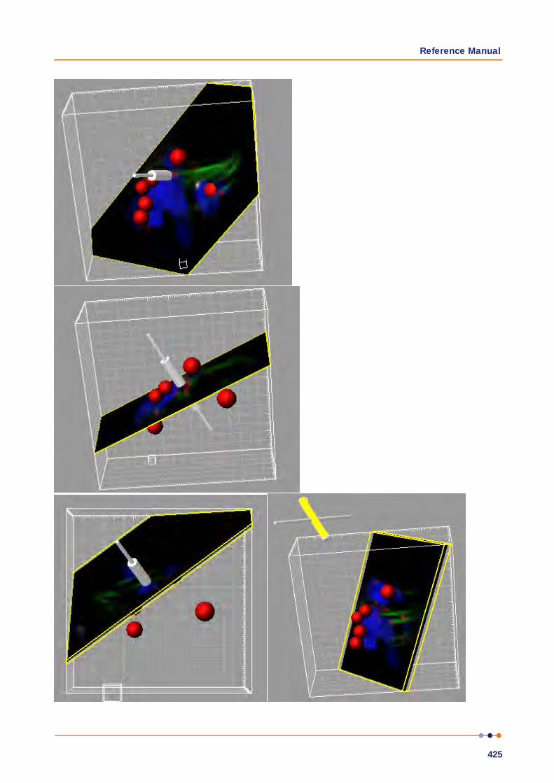
Reference Manual

425

IMARIS

426

How to Add a new Oblique Slicer?

Select menu 3D View - Oblique Slicer.

The Surpass Tree list is automatically updated and in the Oblique Slicer - Properties the Settings parameter are

displayed. The Oblique Slicer is displayed in the viewing area (depending on the default parameter on the tab

Settings).

Change Position of the Oblique Slicer

The Oblique Slicer can be freely moved and rotated to any angle and depth, allowing you complete control over

which portion of the data set is visible and which portion is hidden.

To move and rotate the data set within the viewing area, the pointer must be in the Select mode.

To move the Oblique Slicer in the viewing area and click on the bigger diameter rod. It will turn colored as it is

selected, move it to set the Oblique Slicer to the required position.

Rotate Oblique Slicer around Axes

The Oblique Slicer can be rotated around the x-, y-, and the z-axes. In Select mode click the smaller diameter

rod. It will be highlighted as it is selected. To rotate the Oblique Slicer, move the smaller rod.


Under the Setting tab you can adjust the position and orientation of the Oblique Slicer, adjust the slice

thickness and control the visibility of the Frame.

Orientation

Button YZ Plane

Button XZ Plane

Button XY Plane

Change the Slicer direction, if required, by selecting the adequate plane.

Position

Button Recenter

Click on this button to re-center the Slicer.

Extended Section

The section is a single cut through the data set, the highlighted lines indicate the frame around the active slice.

In the data field you can adjust the distance between the two lines.

Show Frame

Check the box to display a colored frame around the Slicer.

Camera

Button Orthogonal View

The camera is set to a position which is perpendicular to the Slicer.

Reference Manual

427


Oblique Slicer Mouse & Keyboard Functions

Left-click on the bigger diameter rod & drag Move plane to desired position

Left-click on the smaller diameter rod & drag Rotate plane to desired position

See also:



Oblique Slicer Mouse & Keyboard Functions

Click on the bigger diameter rod & drag Move plane to desired position

Click on the smaller diameter rod & drag Rotate plane to desired position

See also:


11.12 Ortho SlicerOrtho Slicer represent an orthogonal plane (orthogonal to the coordinate axis of the data set) that can be moved

within the data set. When adding slices, within the Surpass view per default suggested are the directions z, x,

and y as sequence for the first three and all subsequent slices.

How to Add a new Ortho Slicer?

Select menu 3D View - Ortho Slicer.

The Surpass Tree list is automatically updated and in the Ortho Slicer - Properties the Settings parameter are

displayed. The first Slice is displayed in the viewing area (depending on the default parameter on the tab

Settings).


Slice Orientation

YZ Plane

XZ Plane

XY Plane

The check XY, XZ and YZ plane, to select the visibility of the corresponding slice.

Extended Section

The section is a single cut through the data set, the colored lines indicate the frame around the active slice. In

the data field you can adjust the distance between the two lines.

Show Frame

Check the box to display a colored frame around the active slice.

IMARIS

428

Slice Position

Slider

Choose the relative position of the Slice in the data set by means of the slider or a direct entry of the slice

position given as the offset distance from the data set origin (equals the absolute coordinates).


Ortho Slicer Mouse & Keyboard Functions

Left-click plane & drag Change slice position

Right-click plane Change slice orientation

Num plus Increase the extended section

Num minus Decrease the extended section



See also:



Ortho Slicer Mouse & Keyboard Functions

Click plane & drag Change slice position

Ctrl + click plane Change slice orientation

Num plus Increase the extended section

Num minus Decrease the extended section

See also:


11.13 SpotsThe Spots object is available to model point-like structures in the data. It provides a procedure to automatically

detect point-like structures, an editor to manually correct detection errors, a viewer to visualize the point-like

structures as spheres, and statistics output.

How to Add new Spots?

Select menu 3D View - Spots.

The Surpass Tree list is automatically updated and the first window of the Creation Wizard displays in the

Spots - Properties.

See also:


For information on statistics calculations used refer to Spots

Reference Manual

429





In the first window of the Spots Creation Wizard, you will find the algorithm settings. Here, you have to decide, if



Parameters option.

In the first window of the Creation Wizard you find the algorithm settings. Here you have to decide, if you want

to segment only a Region of Interest (ROI), if you want to use the Region Growing for the Spots detection,

and if you want to create Tracks after the Spots detection.

For further details please refer to Section Algorithm, Region of Interest, Source Channel, Classify Spots, Spots

Region Type, Spots Regions, Edit Spots, Tracking, and Classify Tracks.

11.13.1.1 AlgorithmAlgorithm Settings

Note: If you do not want to use the automatic spots creation wizard select the Skip automatic

creation, edit manually button.


Terminates the creation wizard and activates the manual Spots creation.



The Favourite Creation Parameters option is only available if the set of creation parameters has already been

saved under the Creation Tab using the Remember Parameters button.





image segmentation.









IMARIS

430




Process entire Image finally this option appears only, if Segment only a Region of Interest is checked.


parameters (Complete ROI). Uncheck this box and only the region of interest is processed.

Different Spots Sizes (Region Growing)

Check this box if you want to apply the region growing, starting on the tab Spots Region Type.

Track Spots (over Time)

Check this box if you want to track Spots over time, for details please refer to tab Tracking.

Spots Wizard Buttons

Button Back

This button is grayed in the first window of the Creation Wizard.

Button Next


Button Finish

Click on Finish to calculate the desired Spots and display the Spots in the viewing area.

Button Cancel

If you do not want to create Spots click on Cancel.

11.13.1.2 Region of InterestRegion of Interest 1

Here you define the region of interest (ROI). Parameters such as width, height and location of the ROI are used


X, Y, Z, Time

Min, Max, Size




Size of the ROI:







Memory Usage:


Reference Manual

431

Regions of Interest



Button Add



Button Delete


Total Memory Usage:



Button Back


Button Next


Button Finish


Button Cancel

If you do not want to create Spots automatically click on Cancel.

See also:

Surpass View - Overview - Camera Toolbar (change to pointer mode Select)

11.13.1.3 Source ChannelSource Channel

Select the respective source channel, from which the Spots are to be computed.

Spots Detection

Estimated XY Diameter

This parameter specifies the dimension of the Spots object in the X and Y direction. Objects with size smaller

than the specified Estimated Diameter are not detected. The values are reported under the statistics tab as

separate variables.

By default the radius X and Y are equal.

Detect Ellipsoids

IMARIS

432

To change the detection and creation of the spherical Spots objects to ellipsoid shape objects select the

Detect Ellipsoids box.

Check the Detect Ellipsoids box to activate the Estimate Z Diameter field.

If both the Detect Ellipsoids and and Different Spots Sizes (Region Growing) options are selected, the

value entered in the estimated diameter field is used only to determine the position of the spots.

The spot sizes are finally determined by the region growing parameters (Region Growing type and Regions

threshold).

Estimate Z Diameter

This parameter specifies the dimension of the Spots object in the Z direction. Objects with size smaller than

specified Estimated Diameter are not detected. This value is reported under the Statistics tab as a separate

variable.

The value of the specified Z diameter in comparison to the XY diameter determines the overall object shape.

If Z < X,Y the created shape is an oblate spheroid

If Z > X,Y then the r the created shape is a prolate spheroid

If Z = X,Y then the diameter the created shape is a perfect sphere

Background Object Subtraction

If checked, the background will be removed prior to Spots detection. Technically background subtraction

smoothes the image. The intensity is the one of a Gaussian filtered channel (Gaussian filtered by 3/4) minus

the intensity of the original channel Gaussian filtered by 8/9 of sphere radius.


Button Back


Button Next


Button Finish


Button Cancel


11.13.1.4 Classify SpotsSpots filtering is incorporated into the creation process.

Filters allow the removal of objects that would interfere with interpretation of results.

Quality: The 'Quality' is the intensity at the center of the spot in the channel the Spots was detected.

If 'Background Subtraction' was not checked this is the intensity of the channel Gaussian filtered by

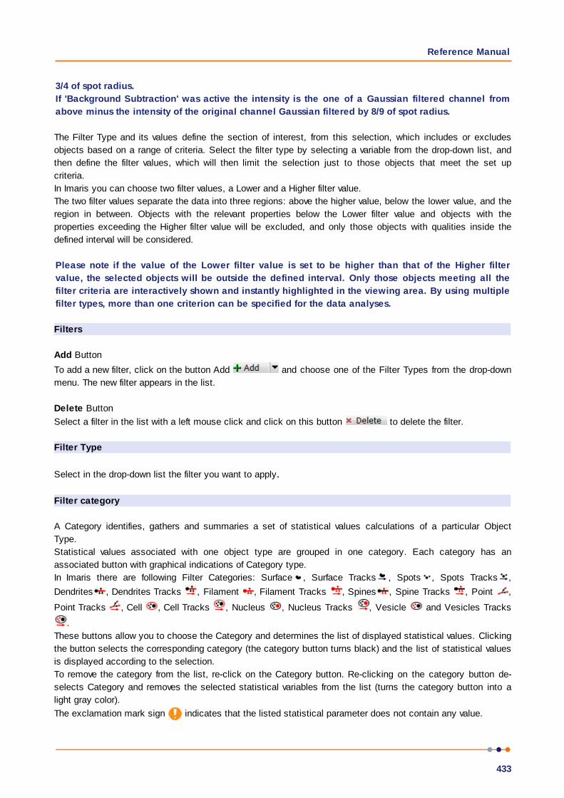
Reference Manual

433

3/4 of spot radius.

If 'Background Subtraction' was active the intensity is the one of a Gaussian filtered channel from

above minus the intensity of the original channel Gaussian filtered by 8/9 of spot radius.




criteria.










Filters

Add Button



Delete Button


Filter Type

Select in the drop-down list the filter you want to apply.

Filter category


Type.






.






light gray color).


IMARIS

434




active threshold.


circle again.



adjustment.










Lower Threshold

Automatic


Manual



visualized.

Higher Threshold

Automatic


Manual



visualized.

Histogram



By clicking into the histogram you move the colored line and the reduced/enlarged set of objects. To change

the Lower threshold value left click on the histogram and drag the yellow line.



Reference Manual

435



Surfaces) is displayed at the bottom of the threshold histogram.





Button Back


Button Next


Button Finish


Button Cancel


11.13.1.5 Spot Region TypeThis tab only appears, if Different Spot Sizes (Region Growing) is checked (Algorithm Settings).

The region method for segmentation in Imaris starts with defined seed points. You use Spots as seed points for

the region growing that is performed in the next steps. During the region growing process around each seed

point the region grows until a border stops the growing.

Spots Regions from

Absolute Intensity

Local Contrast

You can set the border using the Absolute Intensity or the Local Contrast as criteria. In both cases as next

step the selected channel is displayed in the viewing area.

Local Contrast

This option should only be used when the Absolute Intensity method does not properly segment all objects.

Please note: Local Contrast applies a Gaussian filter in order to estimate the intensity value of each voxel.

Baseline Subtraction is then performed by subtracting the variable background from every voxel in the image.

As a result, it uses more memory than the Absolute Intensity method.

Gaussian Smoothing replaces the voxel intensity value with a newly calculated value. The new value is a

IMARIS

436

weighted sum, defined using a Gaussian function, of the voxel and it neighbouring voxels.

The degree of the smoothing is directly dependent on the shape of this kernel, which in turn is a function of the

standard deviation. A Gaussian kernel is a symmetric bell shaped curve.

Absolute Intensity Local Contrast


Button Back


Button Next


Button Finish


Button Cancel


11.13.1.6 Regions ThresholdThis tab only appears, if Different Spots Sizes (Region Growing) is checked (Algorithm Settings).

Spots Regions

The working channel is visualized in the viewing area, the histogram is displayed in the properties area. Regions

above the threshold are displayed in white, regions below threshold are displayed in black. Depending on the

previously selected detection method (Absolute Intensity or Local Contrast) refer to Absolute Intensity or Local

Reference Manual

437

Contrast.

Threshold



adjustment.










Absolute Intensity

Automatic

In the working channel a copy of the intensity histogram of the source channel is displayed. Regions above the

threshold are displayed in white. Now you adjust the threshold of the working channel. Edit the data field or

adjust the threshold manually using the mouse (click & drag the line in the histogram). In the next step the

regions will grow until they fill the white regions and reach the border.

Local Contrast

Automatic

In the selected channel the regions with a local contrast brighter than the background are displayed in white.

Now you adjust the threshold value of the local contrast channel. Edit the data field or adjust the threshold

manually using the mouse (click & drag the line in the histogram). In the next step the regions will grow until

they fill the white regions and reach the border.

Diameter from

Region Volume

The Spot(s) radius is calculated from the region volume (the region volume and the Spots volume are equal).

Region Border

The radius of the calculated Spot(s) is the smallest distance from each Spot center to the region border.

Create Color Coded Region Channel

Additionally the Spots the Region Channel is displayed. Each region has a different color.


Button Back


IMARIS

438

Button Next


Button Finish


Button Cancel


11.13.1.7 Edit SpotsTip: In the Surpass view be sure that the mouse is in the pointer mode Navigate. Switch between the

two pointer modes Select/Navigate with the ESC-key.

AutoDepth Draw

Intersect with

The auto depth function will automatically calculate the Spots depth. Here you select, in which channel or on

which objects Imaris calculates the depth position of the inserted Spots.

all visible Channel

specific Channel - selected channel will be used for Spots depth computation

solid Objects

Select as reference for the Spots depth the first visible channel, all visible channels, or other solid objects.

Process Selection

PC: Mac:

Select spot Left-click Click

Select multiple Spots Ctrl + left-click Command + click

Add new spot Shift + left-click Shift + click

Delete spot Left-click to select, then

click on the button Delete

or

Shift + left-click on a

selected spot

Click to select, then click

on the button Delete

or

Shift + click on a selected

spot

Change spot diameter Mouse wheel Mouse wheel

Button Duplicate

Click this button and all selected Spots appear in a new Surpass Group in the Surpass Tree (Spots Selection).

Button Recenter

Click on the Recenter button results in change of the selected Spots position. The new center is placed in

position of the local intensity maximum in the vicinity of the initial spot center.

Button Delete

Click on this button to delete the selected Spot(s).

Reference Manual

439

Button Clear

Click this button to clear the Spots selection.

No Spots Selected/Selected Spots

Position X: Y: Z: [um]

Display of the Spots position.

Diameter [um]

The initial Spots diameter of a new Spot is the minimum diameter in the creation process. With this parameter

you can change the size.

Time Index

The number indicates the current time point in the series for the selected object.

Spots

In Imaris it its possible to merge two or several Spots items into one Spots item.

Button Merge ...

This button is only available if you have two or more Spots items in the Surpass Tree. Click on this button and

the window Merge selected Objects to "Spots X" displays (see below).

Window: Merge selected Objects to "Spots X"

Check the boxes in front of the desired Spots items or use the button Select All.

Button Clear All

Use this button to clear the Spots selection.

Button OK

If you want to merge the Spots click on OK.

Button Cancel

If you do not want to merge the Spots click on Cancel.

Mask Properties

Sometimes it is useful to apply a certain function not on the entire image but only in a region of interest (ROI).

As region of interest you can choose Spots.

Mask All... Button

Mask Selection ... Button

Here you decide, if the masking is based on selected objects or on all objects. The window Mask Channel

displays (see below).

Window: Mask Channel

Channel Selection

IMARIS

440

Select the channel (destination channel) you want to mask with the Surfaces (ROI).

Duplicate Channel before applying Mask

When this option is selected, the channel will be duplicated before applying Mask.

Mask Settings

Random Color Map

Constant Inside/Outside

Define, if you want to use a random color map or if you want to set a constant inside/outside.

Set Voxels outside Surface to:

The default value is 0.000, no voxels outside the region of interest are displayed.

Set Voxels inside Surface to:

If you leave the box unchecked the original channel intensities inside the region of interest are displayed. If you

check the box and type in 0.000, no voxels inside the region of interest are displayed (no masking!).

Apply to all Time Points

Only available if you work with a time data set. Check the box if you want to apply the mask to all time points.

If the Surfaces changes size and position through the time points the applied mask changes size and position,

respectively.


Button Back


Button Next


Button Finish


Button Cancel

If you do not want to create Tracks click on Cancel.

11.13.1.8 TrackingTracking allows objects to be traced throughout sequential frames of a time data sets, so each object

maintains a unique identity in the output measurements.

This tab only appears, if Track Spots (over Time) is checked (Algorithm Settings).

Algorithm

The Tracking tab provides several tracking algorithms to choose from. The motion models are used to predict

the future positions of Spots. Based on these predicted positions, the best matches to candidate Spots can be

determined. All of the algorithms except for Connected Components use a Linear Assignment algorithm and

Total Cost function to find the best track connections. The first two algorithms compute cost based on change

in position (distance), while Autoregressive Expert mode combines changes in position and intensity to

compute total cost.

Reference Manual

441

Brownian Motion

This algorithm models the motion of each Spot as a Brownian motion. This model is appropriate if your Spots

perform similar to a Brownian motion (the random movement of Spots with very frequent changes in direction

and no discernible pattern).

The only prediction applied is that the Spot does not move further than the specified speed allows, so the



This algorithm models the motion of each Spot as an autoregressive AR1 process. This model is appropriate if

your Spots perform any kind of continuous motion. The AR1 model looks back to one time-point, and predicts

that the Spot will move again the same distance and in the same direction. The user-specified Maximum

Distance value is the distance in which the Spot is allowed to deviate from the predicted position. Some

changes in direction are tolerated because of the maximum distance parameter, and because AR1 does not

remember farther back than one time-point.


This algorithm models the motion of each Spot as an autoregressive AR1 process (see above). It is suitable for

tracing of multiple objects with adjacent or crossing paths, especially if the neighboring objects have a stable

(but different) intensity. In Autoregressive Motion Expert the algorithm called Total Cost determines the most

appropriate connections for tracks by seeking the lowest Total Cost. In this case, the Total Cost algorithm

combines Intensity Cost and Distance Cost functions (see Intensity Weight below).


For this algorithm, Spots in adjacent time-points are considered connected if the Spot spheres occupy some of

the same space (the spheres would overlap if two time-points were merged into one). It compares the amount of

overlaps between identified objects in the previous frame with those in the current frame. All the object with the

overlap will be assigned the same track ID.

Connected Components and Lineage are the only algorithms that automatically handle lineage (spots that

diverge). It will only work with images that have excellent time resolution, because the Spot cannot ever jump a

distance larger than its own size.

Lineage


analyzed. This algorithm models the motion of each object as an autoregressive AR1 process (refer to

Autoregressive Motion above). The object data is then compared so that only the objects that undergo splitting

are connected, and assigned the same track ID. Objects that pass in close proximity, or overlap, are not

associated. This is in contrast to connected components, where any objects that overlap are determined and

considered connected.

Parameters

Max Distance

A maximum distance disallows the connection between a spot and a candidate match if the distance between

the predicted future position of the spot and the candidate position exceeds the defined maximum distance.

The parameter is only available if you select Brownian Motion, Autoregressive Motion, or Autoregressive Motion

Expert (see above).

Max Gap Size


the creation of Track fractions.

IMARIS

442





missing in order for a track to continue.

This parameter is only available if you select Autoregressive Motion or Autoregressive Motion Expert (see

above).






Intensity Weight

Based on the information obtained from the measured Spots intensity and position, the Intensity Weight

function is used to balance the relative influence of the Intensity and Distance costs. The Total Cost is

determined by combining the Intensity term and Distance term, and minimization of the Total Cost is used to

determine the best track from all feasible ones.

TotalCost = (all connections) DistanceCost + IntensityWeight * IntensityCost

The parameter is only available if you select Autoregressive Motion Expert (see above).


Button Back


Button Next


Button Finish


Button Cancel

If you do not want to create Tracks automatically click on Cancel.

Lineage

Table Layout


Reference Manual

443

Time indicator


Track


there may be a number of branch points. The branch points indicate where objects diverge, e.g. cells


Object






When you click on an individual column, the editing table highlights the corresponding object in the image.


track (column in the table) is highlighted.



is selected.



Zoom


or less ("zoom in") of the track-editing table. Using the mouse wheel will have the same effect.

Pan



IMARIS

444

Mouse Selects


Object




Segment


Branch


Pivot





Track


Editing


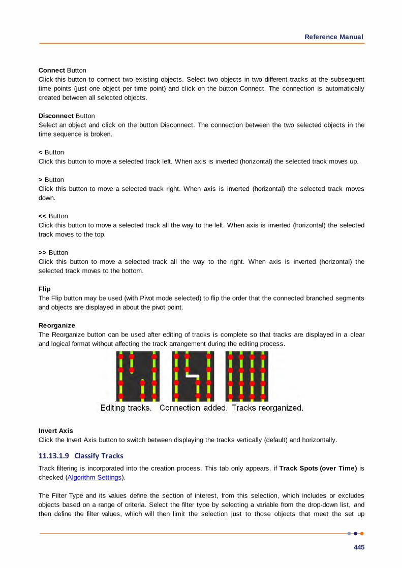
Reference Manual

445

Connect Button

Click this button to connect two existing objects. Select two objects in two different tracks at the subsequent

time points (just one object per time point) and click on the button Connect. The connection is automatically

created between all selected objects.

Disconnect Button

Select an object and click on the button Disconnect. The connection between the two selected objects in the

time sequence is broken.

< Button


> Button


down.

<< Button



>> Button



Flip



Reorganize



Invert Axis


11.13.1.9 Classify TracksTrack filtering is incorporated into the creation process. This tab only appears, if Track Spots (over Time) is

checked (Algorithm Settings).




IMARIS

446

criteria.










Filters

Add Button



Delete Button


Filter Type


Filter category


Type.






.






light gray color).





active threshold.


Reference Manual

447

circle again.



adjustment.










Lower Threshold

Automatic


Manual



visualized.

Higher Threshold

Automatic


Manual



visualized.

Histogram













IMARIS

448


Button Back


Button Next


Button Finish


Button Cancel

If you do not want to create Tracks click on Cancel.

11.13.1.10 Complete ROIThis tab only appears, if Process entire Image finally is checked (Algorithm Settings).

Region of Interest

The parameters you have set up will now be used to compute Spots (and Tracks) for the entire data set.



Button Back


Button Next


Button Finish


Button Cancel

If you do not want to create Spots/Tracks click on Cancel.


On the tab Settings you can adjust the rendering quality to produce faster performance of the display when thenumber of Spots is very large. The size of the Spots can be changed via the Radius Scale box.

Spots Style/Quality

Off

Select this option to disable the visualization of the Spots.

Sphere

This option displays the Spots as as spheres.

Reference Manual

449

Center Point

This option displays the Spots as center points.

Please note: The computation of Spheres is time consuming. If you have many Spots in your data set

Imaris automatically switches to the display mode Center Points. If you would like to switch to the

Spheres mode again select Sphere and confirm the changes.



Off


Line

This option displays the tracks connections dawn as lines.

Cylinder

This option displays the tracks connections dawn as cylinders.

Width

Diameter


Render Quality


Tracks Path

Color Editor

Select a desired color for the Track display.

Displacement



Radius Scale


Color Editor


Dragon Tail



Slider


Subvolume

IMARIS

450

The option Subvolume is used to identify the different objects and distinguish them from the surrounding by

visualizing the volume around a created object. It extracts a subset of the volume data set by using the

specified axis-aligned limits.

The border around each object is defined independently and corresponds to the regions equal to bounding box

of the created object.

MIP

In the Maximum Intensity Projection mode only the point with maximum intensity of all layers along the viewing

direction displayed. If your data set has more then one channel, the combination color is displayed.

Blend

This option displays the subvolume around a certain object in the Blend mode. In the blend mode, all values

along the viewing direction including their transparency are used for the calculation.

11.13.3 Tab Rebuild

Rebuild

Imaris stores the list of operations and the mapping of parameters. Select from the list on which step of the

Spots Creation Wizard you want to re-enter the creation process.


Menu 3D View - Spots - Creation Wizard - Algorithm

Menu 3D View - Spots - Creation Wizard - Region Growing

Menu 3D View - Spots - Creation Wizard - Tracking

Button Rebuild Objects


Creation Parameters

The Creation Wizard saves parameters and processing instructions so the Spots computation can be repeated

for the same region, a different region, or the entire image. Creation Parameters commands are listed.






Arena


Arena







Reference Manual

451








it.









11.13.4 Tab Edit

Once the Spots creation wizard is completed, use these buttons for manual editing of the Spot objects. It

allows you:

1. To add Spots and incorporate them into analysis.

2. To delete selected Spots.

3. Create tracks from Selection

4. Merge selected spots.

Tip: In the Surpass view be sure that the mouse is in the pointer mode Navigate. Switch between the


Add/Delete (Cursor intersects with):

All visible Channels

The All-visible channel option places a spot at the cursor position while the depth through the volume is

determined by the most intense voxel of all the channels

Specific Channel

Select the required channel from the drop-down list and selected channel will be used for Spots computation.

A new spot will be placed at the most intense voxel of the selected channel, even if that channel is overlaid with

other channels of higher intensity.

Surface of Object

Select this option and a new spot will be placed on the surface of an object.

Center of Object

Select this option and a spot will be placed in the center of the object.

IMARIS

452

For Spots object (also Vesicles and dendrite/spines beginning, branching, attaching, terminal points): Select

this option and a new measurement point is placed at the center of the sphere.

Selection

Select between a pointer, circle or box shaped selection.

The pointer mode provides the normal pointer function making it easy to select specific individual spots,

In circle mode a 2D circle appears around the mouse pointer on the screen. Press left-click to select all the

spots that have center points within the circle. Press Ctrl+left-click will add spots to the existing selection, if

some unselected spots are within the circle, otherwise it will deselect all spots within the circle. Use the mouse

wheel to adjust the size of the on-screen selection circle.

In box mode a 3D box appears on the screen around the mouse pointer. Use left-click or Ctrl+left-click the

spots that have center points within the 3D box to add or remove them from the selection.

PC: Mac:

Select Spot Left-click Click


Add new Spot Shift + left-click Shift + click

Delete Spot Left-click to select, then


or


selected Spot



or


Spot

Change Spot diameter Mouse wheel Mouse wheel

Clear Button

Click this button to clear the Spot selection.

Delete Button

Click on this button to delete the selected Spot(s).

Duplicate Button

Click this button and all selected Spots appear in a new Surpass Group in the Surpass Tree (Spots Selection).

Recenter Button

Clicking on the Recenter button changes the position of the selected Spots. The new center is placed in the

position of the local intensity maximum, which is in the vicinity of the initial spot center.

Mask button

Click this button to define the mask functions for the current selection- see Mask Channel section for more

details.

Create Track from Selection Button

Clicking this button creates a track for the selected Spot(s) - see the Create Track from Selection section for

more details

Reference Manual

453

No Spot Selected/Selected Spot

Position X: Y: Z: [um]

Display of the Spot position.

Diameter [um]

The initial Spots diameter of a new Spot is the minimum diameter in the creation process. With this parameter

you can change the size.

Time Index

The number indicates the current time point in the series for the selected object.

Edit All

Merge selected Objects to "Spots X" Button

Click this button to combine multiple spot objects into a single spot item. See the Merge selected Objects to

"Spots X" section for more details.

Mask... button

Click this button to define the mask functions for the image- see Mask Channel section for more details.

Manual Tracking

The Manual Tracking option can either be used when automatic tracking algorithms require modifications and

adjustments, or to create an entire track from scratch.

The manual tracking option allows you to track objects within a time-resolved data set by manually specifying

the object location in each time point. Essentially, the manual tracking is done by clicking on the structure in

the image, which serves as a visual reference (template).

This option can be activated by clicking in the box Auto-connect to selected spot.

To start manual tracking, move the time slider to the first time point of the feature you want to track. Then use

the pointer to Shift and then left click on the feature in the data set.

After each mouse click, the time slider advances one frame, allowing you to see the subsequent image of the

temporal stack. To continue manual tracking, keep clicking on the structure on the image. As you add more

manual tracking points by clicking within the viewing area, a track is created allowing you to follow the moving

features, frame by frame and from point to point, until you’ve built a complete motion path.

Please note: Manual tracking behaviour is governed by the Selection mode under Track Edit tab.

Auto-connect to the selected spot box

Select the option to add all selected or added objects to one track and advance to next time point when a new

object is added or an existing is selected.

Please note: Objects are always added at the current time point (t).

The result of Manual tracking can be very different depending on which selection is chosen in the Track Edit

IMARIS

454

tab.

If the option Track is selected, a connection is established between added object at time point t and the last

added object of the selected track at time point t-1.

If the option Spots is selected, a connection is established between the selected object at the immediately

preceding time point (t-1) and the newly added object at time point t.

Please note: If there is no the immediately preceding time point, a new track will be constructed.

The box on the drawing plane represents the created object diameter. The diameter of the object can be

changed, during the manual tracking, by using the mouse wheel. Use the mouse wheel to increase/decrease

the radius of the created object.

Enable Delay before auto-advancing

The Enable Delay before auto advancing option sets a delay before proceeding to the next time point. When

this option is selected, the created object will be displayed for the duration of the delay in the viewing area. The

visual feedback of the created object gives you an opportunity to adjust it.

The delay duration is adjustable under the Edit menu/Preference/Surpass. You can specify the value between

0.05 and 5 seconds.



11.13.4.1 Mask ChannelChannel Selection




Mask Settings

Random Color Map











respectively.

Button OK

Reference Manual

455

If you want to apply the mask click on OK.

Button Cancel

If you do not want to apply the mask click on Cancel.

11.13.4.2 Merge selected Objects to "Spots X" FunctionCheck the boxes in front of the desired Spots items or use the button Select All.

Button OK

If you want to merge the selected spot objects click on OK.

Button Cancel

If you do not want to merge the selected spot objects click on Cancel.

11.13.4.3 Create Track from Selection1. Select the Source channel

2. Spot Detection

Estimated Diameter

This is the diameter of the inserted Spots. Spots with a diameter smaller than this are not detected.

There are two options for a Surface creation Threshold:


If checked, the background will be removed prior to spot detection.

3.Tracking algorithm


the future positions of Spots. Based on these predicted positions the best matches to candidate Spots can be

determined.

There are two algorithms to choose from:

Brownian Motion

This algorithm models the motion of each Spot as a Brownian motion. This model is appropriate if your Spots

perform similar to a Brownian motion (the random movement of Spots with very frequent changes in direction

and no discernible pattern).

The only prediction applied is that the Spot does not move further than the specified speed allows, so the



This algorithm models the motion of each Spot as an autoregressive AR1 process. This model is appropriate if

your Spots perform any kind of continuous motion. The AR1 model looks back to one time-point, and predicts

that the Spot will move again the same distance and in the same direction . The user-specified Maximum

Distance value is the distance in which the Spot is allowed to deviate from the predicted position. Some

changes in direction are tolerated because of the maximum distance parameter, and because AR1 does not

remember farther back than one time-point.

Lineage

4. Max Distance

The maximum search distance that a tracked object are looked for is specified with the Max Distance value.The parameter Maximum Distance disallows connections between a Spot and a candidate match if thedistance between the predicted future position of the Spot and the candidate position exceeds the maximumdistance.

IMARIS

456

5. Max Gap Size








6. End Time Point

The parameter specifies the last time point for the tracking algorithm implementation.

OK Button

Cancel Button


Mouse Selects




Object

Segment

Branch

Pivot

Track

The differences between these options is described in Tracking.



Table Layout






Object ID

If the mouse pointer is on the object, a tooltip appears that identifies the object ID. The ID numbers of the

objects are sequentially ordered column-wise from the top to the bottom of the table. The object maintains its

unique ID number independent of the track being allocated to.

If the mouse pointer is on the connection, a tooltip appears that identifies the track ID number.

Reference Manual

457







is selected.



Zoom




Pan



Time indicator


The current time point is indicated by vertical line highlighted with in current selection color.





Double-clicking on the time indicator, fixes the position of the current time point at the center of the track-

editing table, regardless of the selected zoom or pan options)

Editing

Track Editor has several features that help you modify your tracks.

Connect Button






Disconnect Button






< Button


IMARIS

458

> Button


down.

<< Button



>> Button



Flip



Reorganize



Invert Axis


Correct Drift



Algorithms


drift.

Translation






Reference Manual

459





Result DataSet size



new image.





result.








Correct spots positions

Activate this parameter and the spots are automatically re-positioned after the drift correction. If this option is




11.13.6 Tab Filter





criteria.





IMARIS

460






Filters

Add Button




Delete Button


Filter Type


Filter category


Type.






.






light gray color).





active threshold.


circle again.


Reference Manual

461


adjustment.










Lower Threshold

Automatic


Manual



visualized.

Higher Threshold

Automatic


Manual



visualized.

Histogram



Manual. By clicking into the histogram you move the colored line and a reduced/enlarged set of the selected

objects. To change the Lower threshold value left click on the histogram and drag the yellow line.





Spots) is displayed at the bottom of the threshold histogram.




Button Duplicate Selection to New Spots


Surpass Tree.

IMARIS

462


Spots statistics are automatically computed. For the statistical values please refer to the Section Menu Edit -

Preferences... - Statistics -Spots. The Statistics tab collects and displays the image's statistical values in





a) Overall

b) Detailed

c) Selection




Overall Tab



Category


Type.






.






light gray color).


Detailed Tab

A pull down list offers three types of Detailed statistical calculations:

Specific Values

Average Values

Time Plots






Reference Manual

463


one.





Specific Values




Average values










Unit- variable unit

Level/Distance







are displayed per time point. The changing the time points, statistical variable values and images are

consequently changed.



Selection Tab


Specific Values

Average Values

Time Plots





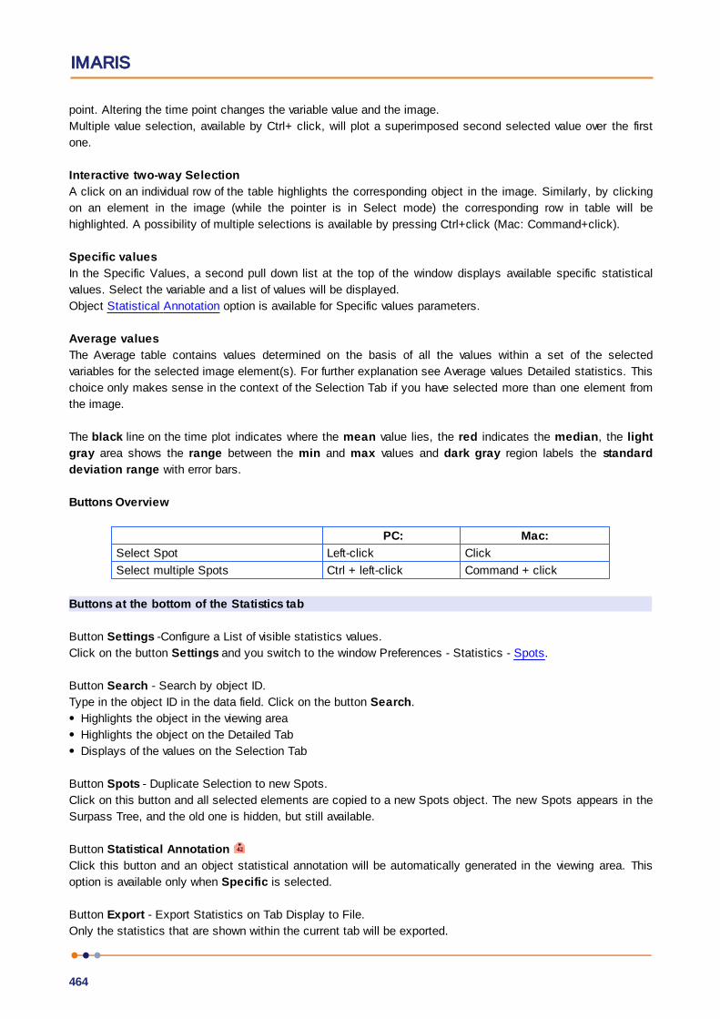
IMARIS

464



one.





Specific values




Average values




the image.




Buttons Overview

PC: Mac:

Select Spot Left-click Click




Click on the button Settings and you switch to the window Preferences - Statistics - Spots.






Button Spots - Duplicate Selection to new Spots.

Click on this button and all selected elements are copied to a new Spots object. The new Spots appears in the

Surpass Tree, and the old one is hidden, but still available.



option is available only when Specific is selected.



Reference Manual

465





automatically.



When the Selection tab is selected, pressing the Export all Statistics to File button, will export all the statistics

(that are enabled in the statistics settings) of all the selected objects, not all the statistics of all the objects.




See also:

Menu Edit - Preferences... - Statistics - Spots





The Statistical Annotation button provides a convenient interface in order to label the object with the

statistical data. Click this button and an object statistical annotation will be automatically generated in the

viewing area. The selected object is annotated for all time points with the specified statistical values.





click)

In the Detailed or Selection Tab a pull down list offers Specific Values as the type of statistical parameters.














IMARIS

466



11.13.8 Tab Color

Tab Color edit, manage and assign colors material to the Spots or Tracks.

Object Type

Choice of the Object type is presented in a drop-down window. Select either Point (for Spots) or Tracks and

depending on the chosen object type selection of the variables is listed.

For Object Type Points two color types are available:

Base

Statistics Coded

For Object Type Tracks the following color types are available:

Labels- non-labelled objects are displayed in the Base color.

Base

Statistics Coded

Track ID

Time Mapped

Color Type-Object ID

11.13.8.1 Color Type- LabelsThe labels associated with the data set is displayed as a list.


Transparency



11.13.8.2 Color Type-BaseBase

Assign the Spots/Track color via the Color Editor. Tab Color edit, manage and assign material colors of aSpots/Track.

RGB




Light reflection




Reference Manual

467

applied to the object. The default setting is no specular intensity.


light.

Transparency



Palette








Depending on the chosen object type the Statistical variable selection is listed in the drop-down window. For

example, if Point is chosen as the object type, available Statistical data will be Point linked variable. Similarly,

variables for Tracks will be listed, if the object type is selected to be Tracks.


Statistics colorbar are displayed in the viewing area. The upper one is the colorbar range for Points and lower

one is the colorbar for the Tracks.

Show Colorbar


Show Title


Show Range



Colormap

Button Reset


Colormap




IMARIS

468

Colormap range

Colormap range-specify the limits for the colorbar.



Button Auto

Click the button Auto and the system detects the real min and max values and sets the Max. and Min. limits


Transparency



11.13.8.4 Color Type-Time MappedTime Mapped

This option is only available when Tracks (see above) is selected as Object Type. The color range for the


Transparency



11.13.8.5 Color Type-Object IDAssigns a random color to every object. This is available for all surpass components.




Transparency




Spots Mouse & Keyboard Functions on the Tab Edit

Select Spot Left-click

Select multiple Spots Ctrl + left-click

Add new Spot Shift + left-click

Delete Spot Left-click to select, then click on the button

Delete

Change Spot diameter Mouse wheel

See also:


Reference Manual

469

11.13.10Mouse & Keyboard Mac

Spots Mouse & Keyboard Functions on the Tab Edit

Select Spot Click

Select multiple Spots Command + click

Add new Spot Shift + click

Delete Spot Click to select, then click on the button

Delete

Change Spot diameter Mouse wheel

See also:


11.14 SurfacesThe Surfaces visualization is a computer-generated representation of a specified gray value range in the data

set. It creates an artificial solid object in order to visualize the range of interest of a volume object.

How to Add a new item Surfaces?

Select menu 3D View - Surfaces.

The Surpass Tree list is automatically updated and the first window of the Creation Wizard displays in the

Surfaces - Properties.

For information on statistics calculations used refer to Surfaces





In the first window of the Surface Creation Wizard, you find the algorithm settings. Here, you have to decide, if



Parameters option.

In the first window of the Creation Wizard you find the algorithm settings. Here you can choose to segment a

Region of Interest (ROI) only, to create Tracks after the objects detection, use the Seeded Region

Growing for the Surfaces detection or to Skip automatic creation and start Contour Surface drawing .

If you do not want to use the automatic Surface creation wizard select the Skip automatic creation, edit

manually button.


Terminates the creation wizard and activates the manual Surface creation.

For further details please refer to Section Algorithm, Region of Interest, Source Channel, Threshold, Classify

Seed Points, Classify Surfaces, Tracking, Edit Surfaces, Classify Tracks and Complete ROI.

IMARIS

470

11.14.1.1 Algorithm

Note: If you do not want to use the automatic surface creation wizard select the Skip automatic

creation, edit manually button.


Terminates the creation wizard and activates the manual Surface creation.









image segmentation.






Algorithm Settings







Process entire Image finally this option appears only, if Segment only a Region of Interest is checked.


parameters (Complete ROI). Uncheck this box and only the region of interest is processed.

Track Surfaces (over Time)

Check this box if you want to track the resulting Surfaces over time, for details please refer to tab Tracking.


Button Back

This button is grayed in the first window of the Creation Wizard.

Button Next

Reference Manual

471


Button Finish


Button Cancel


11.14.1.2 Region of InterestRegion of Interest 1

Here you define the region of interest (ROI). Parameters such as width, height and location of the ROI are used


X, Y, Z, Time

Min, Max, Size




Size of the ROI:







Memory Usage:


Regions of Interest



Button Add



Button Delete


Total Memory Usage:


Button Cancel

If you do not want to create Surface click on Cancel.


IMARIS

472

Button Back


Button Next


Button Finish


Button Cancel


11.14.1.3 Source ChannelSource Channel

Select the respective source channel, from which the Surfaces are to be computed.

Smooth


to the data set.



If the option Smooth is selected then the Surface Area Detailed Level value should be determined. Use

either the automatically given value or type in a new value in the data field.

Threshold

There are two options for Surface creation Threshold:

Absolute Intensity

Background Subtraction (Local Contrast)




The width of the Gaussian filter is calculated by subtracting the diameter of the largest sphere that fits into

the Object from the intensity of the original channel.


Sphere Diameter






Reference Manual

473

Button Back


Button Next


Button Finish


Button Cancel


11.14.1.4 ThresholdThreshold

Activating/deactivating the threshold option is done by clicking on the or button. The Red button


threshold.


circle again.



adjustment.

When the threshold values are not activated (the red button ) the corresponding A/M button is light gray

indicating that threshold adjustment is unavailable. When the threshold option is activated (the green

button ), the corresponding A/M button turns black.













considered.

Please note if the value of the Lower threshold is set higher than the value of Higher threshold the selected



IMARIS

474



General

Automatic

The initial threshold value is automatically computed using an algorithm based on [T.W. Ridler and S. Calvard,

"Picture thresholding using an iterative selection method", IEEE Trans. System, Man and Cybernetics, SMC-8

(1978) 630-632].

Manual

Define the requested threshold by clicking into the histogram or by entering the value directly in the data field.

Split touching Objects (Region Growing)

This option supports the separation of two or more objects that are identified as one. The region method for

segmentation in Imaris starts with defined seed points. During the region growing process around each seed

point the region grows until a border stops the growing.

If you want to apply the seeded region growing for the Surfaces creation check the respective option. The

threshold you set above is the border of the region growing.

Seed Points Diameter

Type in the estimated diameter of a seed point.

Preview Region Info

For large data sets that exceed a certain memory limit, a Surface preview is only created for a centred sub-

region for which the volume is

highlighted. The size of the sub-region matches a memory limit defined in the advanced preferences, see

Preferences -> Advanced, the

parameter bpSurfacesModelViewer->3DPreviewMemoryLimitMB for 3D volumes and bpSurfacesModelViewer-

>4DPreviewMemoryLimitMB

for time resolved data. For placing the Surface preview region manually, a ROI needs to be defined.


Button Back


Button Next


Button Finish


Button Cancel


Reference Manual

475

11.14.1.5 Classify Seed PointsThe Seed Points filtering is incorporated into the creation process. This tab only appears, if Split touching

Objects (Region Growing) is checked (Algorithm Settings).

Filtering allows the removal of objects that would otherwise interfere with the interpretation of results.




criteria.






Please note that if the value of the Lower filter value is set to be higher than that of the Higher filter




Filters

Add Button



Delete Button


Filter Type


Filter category


Type.






.






IMARIS

476

light gray color).





active threshold.


circle again.



adjustment.










Lower Threshold

Automatic


Manual



visualized.

Higher Threshold

Automatic


Manual



visualized.

Histogram




Reference Manual

477











Button Back


Button Next


Button Finish


Button Cancel


11.14.1.6 Classify SurfacesThe Surfaces filtering is incorporated into the creation process.

Filters allow the removal of objects that would interfere with interpretation of results.


objects based on a range of criteria. Select the filter type by selecting the required variable from the drop-down

list, and then define the filter values, which will then limit the selection just to those objects that meet the set

criteria.









IMARIS

478


Filters

Add Button



Delete Button


Filter Type


Filter category


Type.






.






light gray color).





active threshold.


circle again.



adjustment.





Reference Manual

479






Lower Threshold

Automatic


Manual



visualized.

Higher Threshold

Automatic


Manual



visualized.

Histogram














Button Back


Button Next


Button Finish

IMARIS

480


Button Cancel


11.14.1.7 Edit SurfacesHere you find the manual editing tools for the Surfaces.



Edit Mode

Add/Delete

This activates a semi-automatic surface segmentation (see below). Single objects can be added by one mouse

click. If you select Add/Delete as edit mode, the Add/Delete Properties are available (see below).

Cut

This activates the Surface Scissors function (see below). You can manually split two touching surface objects.

If you select Cut as edit mode, the Cut Properties are available (see below).

AutoDepth Draw

The auto depth function will automatically calculate the Surface depth. Here you select, in which channel or on

which objects Imaris calculates the depth position of the inserted Surface.

Intersect with:

all visible Channels

specific Channel

solid Objects

Select as reference for the Spot depth the first visible channel, all visible channels, or other solid objects.

Add/Delete Properties

The Add/Delete Properties are only available, if you select Add/Delete as edit mode (see above).

There are two different techniques available:

Marching Cubes

Optimized for objects with a complex rough surface. It runs a marching cube type surface generation process in

the bounding box around the mouse (automatic threshold).

Position the autodepth cursor to the center of the object.

Adjust the size of the box to the approximate size of the object (use the mouse wheel).

Shift + click to create the new object.

Magic Wand

Optimized for single, complex objects, which are located over a larger region of the image. The Magic Wand

algorithm is ideal for the global detection of arbitrarily-shaped objects. It reads the threshold from the cursor

position and creates a surface (same as marching cube but on entire image).

Position the autodepth cursor to the border of the object (the size of the box does not influence the result).

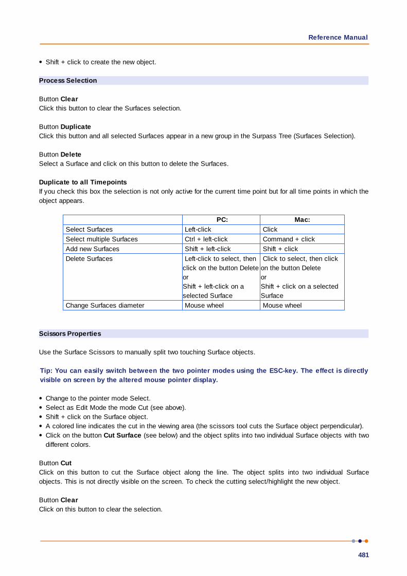
Reference Manual

481


Process Selection

Button Clear

Click this button to clear the Surfaces selection.

Button Duplicate

Click this button and all selected Surfaces appear in a new group in the Surpass Tree (Surfaces Selection).

Button Delete

Select a Surface and click on this button to delete the Surfaces.

Duplicate to all Timepoints

If you check this box the selection is not only active for the current time point but for all time points in which the

object appears.

PC: Mac:

Select Surfaces Left-click Click

Select multiple Surfaces Ctrl + left-click Command + click

Add new Surfaces Shift + left-click Shift + click

Delete Surfaces Left-click to select, then


or


selected Surface



or


Surface

Change Surfaces diameter Mouse wheel Mouse wheel

Scissors Properties

Use the Surface Scissors to manually split two touching Surface objects.



Change to the pointer mode Select.

Select as Edit Mode the mode Cut (see above).

Shift + click on the Surface object.

A colored line indicates the cut in the viewing area (the scissors tool cuts the Surface object perpendicular).

Click on the button Cut Surface (see below) and the object splits into two individual Surface objects with two

different colors.

Button Cut

Click on this button to cut the Surface object along the line. The object splits into two individual Surface

objects. This is not directly visible on the screen. To check the cutting select/highlight the new object.

Button Clear

Click on this button to clear the selection.

IMARIS

482

Close Borders

Check this box to add a surface along the cutting line and close the surface.

Mask Properties

Sometimes it is useful to apply a certain function not on the entire image but only in a region of interest (ROI).

As region of interest you can choose Surfaces.

Button Mask All...

Button Mask Selection ...



Surfaces

In Imaris it its possible to merge two or several Surfaces items into one Surfaces item.

Button Merge ...

This button is only available if you have two or more Surface items in the Surpass Tree. Click on this button and

the window Merge selected Objects to "Surfaces X" displays (see below).


Channel Selection




Mask Settings

Random Color Map











respectively.

Button OK


Reference Manual

483

Button Cancel


Window: Merge selected Objects to "Surfaces X"

Check the boxes in front of the desired Surfaces or use the button Select All.

Button Clear All

Use this button to clear the Surfaces selection.

Button OK

If you want to merge the Surfaces click on OK.

Button Cancel

If you do not want to merge the Surfaces click on Cancel.


Button Back


Button Next


Button Finish


Button Cancel


11.14.1.8 TrackingTracking allows objects to be traced throughout sequential frames of a time data sets, so each object

maintains a unique identity in the output measurements.

This tab only appears, if Track Surfaces (over Time) is checked (Algorithm Settings).

Algorithm


the future positions of Surfaces. Based on these predicted positions the best matches to candidate Surfaces

can be determined. All of the algorithms except for Connected Components use a Linear Assignment algorithm

and Total Cost function to find the best track connections. The first two algorithms compute cost based on

change in position (distance), while Autoregressive Expert mode combines changes in position and intensity to

compute total cost.

Brownian Motion

This algorithm models the motion of each surface as a Brownian motion. This model is appropriate if your

Surface performs similar to a Brownian motion (the random movement of Surface with very frequent changes in

direction and no discernible pattern).

The only prediction applied is that the Surface does not move further than the specified speed allows, so the


IMARIS

484


This algorithm models the motion of each Surface as an autoregressive AR1 process. This model is appropriate

if your Surface perform any kind of continuous motion. The AR1 model looks back to one time-point, and

predicts that the Surface will move again the same distance and in the same direction. The user-specified

Maximum Distance value is the distance in which the Surface is allowed to deviate from the predicted

position. Some changes in direction are tolerated because of the maximum distance parameter, and because

AR1 does not remember farther back than one time-point.


This algorithm models the motion of each Surface as an autoregressive process. This model is appropriate if

your Surfaces perform any kind of continuous motion. In the expert mode the tracks are predicted by the

additionally established algorithm called Intensity Weight (see below).


For this algorithm, Surface objects in adjacent time-points are considered connected if the Surface spheres

occupy some of the same space (the spheres would overlap if two time-points were merged into one). It

compares the amount of overlaps between identified objects in the previous frame with those in the current

frame. All the object with the overlap will be assigned the same track ID. Connected Components and Lineage

are the only algorithms that automatically handle lineage (objects that diverge). It will only work with images

that have excellent time resolution, because the object cannot ever jump a distance larger than its own size.

Lineage


analyzed. This algorithm models the motion of each object as an autoregressive AR1 process (refer to

Autoregressive Motion above). The object data is then compared so that only the objects that undergo splitting

are connected, and assigned the same track ID. Objects that pass in close proximity, or overlap, are not

associated. This is in contrast to connected components, where any objects that overlap are determined and

considered connected.

Parameters

Max Distance

The maximum search distance that a tracked object are looked for is specified with the Max Distance value.

This parameter disallows connections between a Surface and a candidate match if the distance between the

predicted future position of the Surface and the candidate position exceeds the maximum distance.

The parameter is only available if you select Brownian Motion, Autoregressive Motion, or Autoregressive Motion

Expert (see above).

Max Gap Size








The parameter is only available if you select Autoregressive Motion or Autoregressive Motion Expert (see

Reference Manual

485

above).



consecutive time points along the trajectory. If this option is selected, the algorithm performs the optimization of



Intensity Weight

Tracks are computed by minimization of a cost function that combines distance based and intensity based

costs. "Intensity Weight" is the factor by which IntensityCost is taken into account:

TotalCost = sum_(all connections) DistanceCost + IntensityWeith * IntensityCost

The parameter is only available if you select Autoregressive Motion Expert (see above).


Button Back


Button Next


Button Finish


Button Cancel


Lineage

Table Layout


IMARIS

486

Time indicator


Track


there may be a number of branch points. The branch points indicate where objects diverge, e.g. cells


Object






When you click on an individual column, the editing table highlights the corresponding object in the image.


track (column in the table) is highlighted.



is selected.



Zoom


or less ("zoom in") of the track-editing table. Using the mouse wheel will have the same effect.

Pan



Mouse Selects


Object




Segment


Branch


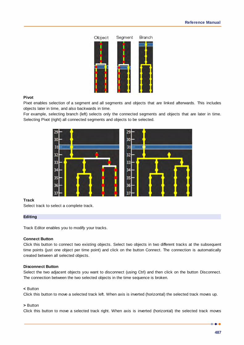
Reference Manual

487

Pivot





Track


Editing


Connect Button

Click this button to connect two existing objects. Select two objects in two different tracks at the subsequent

time points (just one object per time point) and click on the button Connect. The connection is automatically

created between all selected objects.

Disconnect Button

Select the two adjacent objects you want to disconnect (using Ctrl) and then click on the button Disconnect.

The connection between the two selected objects in the time sequence is broken.

< Button


> Button


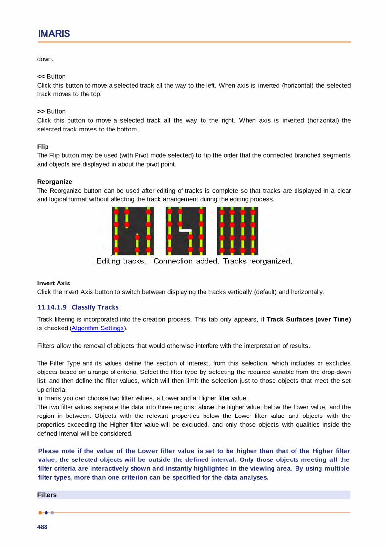
IMARIS

488

down.

<< Button



>> Button



Flip



Reorganize



Invert Axis


11.14.1.9 Classify TracksTrack filtering is incorporated into the creation process. This tab only appears, if Track Surfaces (over Time)

is checked (Algorithm Settings).

Filters allow the removal of objects that would otherwise interfere with the interpretation of results.


objects based on a range of criteria. Select the filter type by selecting the required variable from the drop-down

list, and then define the filter values, which will then limit the selection just to those objects that meet the set

up criteria.










Filters

Reference Manual

489

Add Button



Delete Button


Filter Type


Filter category


Type.






.






light gray color).





active threshold.


circle again.



adjustment.








IMARIS

490



Lower Threshold

Automatic


Manual



visualized.

Higher Threshold

Automatic


Manual



visualized.

Histogram














Button Back


Button Next


Button Finish


Button Cancel

Reference Manual

491


11.14.1.10 Complete ROIThis tab only appears, if Process entire Image finally is checked (Algorithm Settings).

Region of Interest

The parameters you have set up will now be used to compute Surfaces (and Tracks) for the entire data set.



Button Back


Button Next


Button Finish


Button Cancel



Surfaces Style/Quality

Surface

Select this option and the created Surfaces is displayed in the viewing area.

Slicer View

This presents the created Surfaces in a rendered slice view (requires OpenGL 4.0 support). Select the slicer

orientation from the drop-down box.

Center Point

This option displays the Surfaces as center points.

Off

Select this option to disable the visualization of the Surfaces.

Tracks Display

Select how to visualize the tracks:

Full Tracks

Select this option to show the complete track.

Dragon Tail

Select this option to view a dragons tail for the object in motion. The parts of the track ahead and following the

object can be adjusted (in seconds) using the Next and Last fields respectively.

IMARIS

492

Off

Select this option to disable the visualization of the tracks.

Tracks Style

Set the display of connections between the Track objects.

Line


Cylinder


Diameter

Depending on the previous selection you can adjust the width of the line (in pixels) or diameter of the cylinder

(in um) using the slider.

Tracks Displacement Display



Arrow Scale

Adjust the thickness of the displacement arrows by changing the value in the Arrow Scale field.

Color Editor


11.14.3 Tab Rebuild

Rebuild

Imaris stores the list of operations and the mapping of parameters. Select from the list on which step of the

Surfaces Creation Wizard you want to re-enter the creation process.


Menu 3D View - Surfaces - Algorithm

Menu 3D View - Surfaces - Tracking

Rebuild Objects Button


Creation Parameters

The Creation Wizard saves parameters and processing instructions so the Surfaces computation can be

repeated for the same region, a different region, or the entire image. Creation Parameters commands are listed.





Reference Manual

493


Arena


Arena














it.









11.14.4 Tab Draw

The Draw tab allows the user to semi-automatically create further Surface objects.

The Draw tab has two sub tabs:

Add/Delete

Contour



11.14.4.1 Add/DeleteAdd/Delete

This activates a semi-automatic surface segmentation.

Here you select, in which channel or on which objects Imaris calculates the depth position of the inserted

Surface.

IMARIS

494

Intersect with:

all visible Channels

specific Channel

solid Objects

Select as reference for the Surface depth the first visible channel, all visible channels, or other solid objects.

Add Surface using:

There are two different techniques available for adding the Surface Objects:

Marching Cubes

Optimized for objects with a complex rough surface. It runs a marching cube type surface generation process in

the bounding box around the mouse (automatic threshold).

Position the cursor to the center of the object.

Adjust the size of the box to the approximate size of the object (use the mouse wheel).


Magic Wand

Optimized for single, complex objects, which are located over a larger region of the image. The Magic Wand

algorithm is ideal for the global detection of arbitrarily-shaped objects. It reads the threshold from the cursor

position and creates a surface (same as marching cube but on entire image).

Position the cursor to the border of the object (the size of the box does not influence the result).


Manual Tracking

The Manual Tracking option can either be used when automatic tracking algorithms require modifications and

adjustments, or to create an entire track from scratch.

The manual tracking option allows you to track objects within a time-resolved data set by manually specifying

the object location in each time point. Essentially, the manual tracking is done by clicking on the structure in

the image, which serves as a visual reference (template).

This option can be activated by clicking in the box Auto-connect to selected Surface.

To start manual tracking, move the time slider to the first time point of the feature you want to track. Then use

the pointer to Shift and then left click on the feature in the data set.

After each mouse click, the time slider advances one frame, allowing you to see the subsequent image of the

temporal stack. To continue manual tracking, keep clicking on the structure on the image. As you add more

manual tracking points by clicking within the viewing area, a track is created allowing you to follow the moving

features, frame by frame and from point to point, until you’ve built a complete motion path.

Please note: Manual tracking behaviour is governed by the Selection mode under Track Edit tab.

Auto-connect to the selected Surface box

Select the option to add all selected or added objects to one track and advance to next time point when a new

object is added or an existing is selected.

Reference Manual

495

Please note: Objects are always added at the current time point (t).

The result of Manual tracking can be very different depending on which selection is chosen in the Track Edit

tab.

If the option Track is selected, a connection is established between added object at time point t and the last

added object of the selected track at time point t-1.

If the option Surface is selected, a connection is established between the selected object at the immediately

preceding time point (t-1) and the newly added object at time point t.

Please note: If there is no the immediately preceding time point, a new track will be constructed.

The box on the drawing plane represents the created object diameter. The diameter of the object can be

changed, during the manual tracking, by using the mouse wheel. Use the mouse wheel to increase/decrease

the radius of the created object.

Enable Delay before auto-advancing

The Enable Delay before auto advancing option sets a delay before proceeding to the next time point. When

this option is selected, the created object will be displayed for the duration of the delay in the viewing area. The

visual feedback of the created object gives you an opportunity to adjust it.

The delay duration is adjustable under the Edit menu/Preference/Surpass. You can specify the value between

0.05 and 5 seconds.

11.14.4.2 Contour SurfaceThe Contour Surface allows you to extract a 3D object by manually drawing the object contours on 2D slices.

You can employ this method whenever simple threshold does not yield individual structures (e.g. touching cells

in confocal microscopy, complex tissue recorded by transmission microscopy).

It is recommended to uncheck any other object in the Surpass Tree before drawing the contour, so that only the

contour is visible in the viewing area.

The Contour Tab has three sub-tabs:

Board

Mode

Autofit

11.14.4.2.1 Board

A drawing plane is displayed in the viewing area.

Orientation

This option defines the orientation of the drawing plane. Once orientation of the drawing plane is selected, the

drawing planes of all contours are set in the same position. By default the orientation is set to be in the XY

plane-z-direction.

Choose the YZ-plane to draw in the x-direction. Choose the XZ-plane to draw in the y-direction. Choose the XY-

plane to draw in the z-direction.

Visibility

This option defines the Visibility of previously drawn contour lines.

IMARIS

496

None

The contour currently being drawn is made visible.

Next

The contour(s) next to the contour currently drawn is/are shown.

All

All contours are shown.

Resolution

This option controls the smoothness and complexity of the surface created by the contour lines. It can be used

to reduce the number of triangles in a surface object according to a user-defined value. There are two options:

Automatic

The Automatic resolution depends on the contour line vertex spacing.

Manual

The manual resolution is controlled with the slider. Moving the slider to the left reduces the resolution, moving it

to the right increase resolution.

Setting the Resolution to 100% corresponds to the data set resolution. Setting the resolution to 1% reduces

the voxel resolution to 1% of original data set.

Preserve feature

If the box Preserve feature is selected, a Surface calculation is then performed using anisotropic Gaussian

filtering. This feature aims to reduce image noise without removing significant parts of the image content,

ensuring that thin and sharp features are not absent from the created surface. The filter size is calculated

adaptively and separately for each plane. It produces a family of contour lines, and each resulting line is a

combination between the original image and a filter that depends on the local content of the original image. As

a consequence, in the created Surface noise is removed, and significant parts of the image content (like

elongated and narrow features) are preserved.

If the Preserve feature is not selected an isotropic Gaussian filter is used for the Surface creation. The

smoothing is made along the structures, resulting in consistently smooth Surface.

Please note: As a result of applying isotropic Gaussian filter, thin and sharp Surface features may fail

to be created.

Selection

The following button actions apply to the previously created contour lines.

Button Cut

To cut a contour line in a plane click on the button Copy.

Button Copy

To copy a contour line in a plane click on the button Copy.

Button Paste

To paste a contour line in click on the button Paste.

Button Delete

To delete a contour line click on the button Delete

Reference Manual

497

Button Smooth

To smooth a contour line edge click on the button Smooth.

Slice Position

The border of the active drawing plane is shown in your selected color, thus clearly indicating the slice currently

in use. There are several ways to move between slices and select individual slices to create new contours. You

can either:

- Drag the slider handle to the left or right

- Use the up or down arrow keys

- Enter the slice number in the numerical field

Slice (data field)

The respective slice number is displayed in the number field.

The position of slices can be alternatively also changed in the viewing area. Switch the pointers to the Select

mode and then simply click at the drawing plane and drag it to a new position.

Lock button

This option prevents the orthogonal slicer from being accidentally shifted with the mouse during editing or

contour line creation.

Selecting the Lock option generally "constrains" movement of the drawing plane in the viewing area, but it still

allows changes to be made using either the slider options or up/down arrow key.

The L key allows the switch between locked and unlocked orthogonal slicer.

Please refer to the Section Shortcuts Overview in the Reference Manual for a detailed list of shortcuts for

manual surface creation.

Draw button

Click on this button to alter between the two Drawing Modes: Active and Inactive

Drawing Modes

In the contour line, creations there are two different drawing modes: Active and Inactive.ActiveThe main function of the active drawing mode is to create a contour line. The active drawing mode can also beused to insert new vertices into existing contour lines.InactiveIn the inactive drawing mode, the existing contour lines can be modified or deleted.You can select the respective mode by using the Draw button or Ctrl+space key.Press the Draw button or Ctrl+space key to alter Drawing mode between Active and Inactive mode.

The pointer’s appearance on the screen depends on the selected drawing mode. The symbol on the screenchanges from an arrow in the Inactive drawing mode to a cross in the Active mode.

Create Surface button

To create surfaces click on the button Create Surfaces. The Surface item appears in the Surpass Tree and is

displayed in the viewing area.

IMARIS

498

11.14.4.2.2 Mode

Drawing Modes

In the contour line, creations there are two different drawing modes: Active and Inactive.ActiveThe main function of the active drawing mode is to create a contour line. The active drawing mode can also beused to insert new vertices into existing contour lines.InactiveIn the inactive drawing mode, the existing contour lines can be modified or deleted.You can select the respective mode by using the Draw button or Ctrl+Space key.Press the Draw button or Ctrl+Space key to alter Drawing mode between Active and Inactive mode.

The pointer’s appearance on the screen depends on the selected drawing mode. The symbol on the screenchanges from an arrow in the Inactive drawing mode to a cross in the Active mode.

Please refer to the section 'Shortcuts Overview' for a listing of the respective shortcuts.

Several segmentation tools are provided allowing you to select areas in the current slice for contour line

drawing.

Select one of the shape object tools in the Drawing Mode. Left clicking on a tool icon activates a drawing tool.

Once a drawing style tool is selected you may adjust the specific parameters for that drawing mode.

Once a segmentation tool is activated and adjusted, activate the drawing mode by changing the pointer mode

to Select (press the ESC-key) and then once press the Draw button or Ctrl+space key. The Drawing mode is

activated.

By default, contour lines are drawn in a transparent gray color. The color of the contour lines can be modified

using a dialog under the Color Tab.

Click

Clicking within the image inserts a point, a so-called vertex. You can now define subsequent vertices by

clicking with the left mouse button. Successive points will be connected with straight-line segments.

Time

Click once on the contour and then move the mouse along the contour. The number of vertices depends on the

time interval (ms), specified in the corresponding field. The interval can be changed by manually specifying the

required value. This drawing style allows you to draw a structure that contains fine details.

Insert a vertex after ms

The number specifies the time interval (in ms) between two inserted vertices.

Distance

Click once on the contour and then simply move the mouse along the contour. The number of vertices depends

on the distance interval (um), which is specified in the corresponding field. To change the interval, specify the

required value in the object properties area. This drawing style is recommended if the structure is smooth.

Vertex spacing um

The number specifies the distance interval (in um) between inserting two inserted vertices.

Circle

The Circle drawing tool inserts a circular contour line. The Circle tool always draws a contour line from the

center; that is, the place you initially click will be the center point of the contour line. To change the circle

Reference Manual

499

radius specify the required value in the object properties area. In the parameters you can also specify the

number of contour vertices to be inserted. To create the contour line, move the mouse pointer over the

orthogonal slicer plane. A preview outline of the circle is then displayed. To create a contour line, click with the

left mouse button on the desired position.

Radius um

Defines the radius of the circle in um.

Tip: Scrolling the mouse wheel can also change the radius of circle.

Number of vertices

Defines the number of vertices in the circle line.

Isoline

The Isoline drawing tool generates contours at a fixed iso-value so the geometrical features of the contour line

takes into account the image's intensity values. Connecting the points with a constant intensity value forms the

contour line.

The Isoline drawing mode selects the maximum intensity iso-value under the mouse pointer and creates a

contour line by tracing points of uniform intensity. Clicking with the left mouse button on the orthogonal slicer

plane selects the largest connected area that contains the all voxel with the same intensity values. The current

iso-value under the mouse pointer is displayed in the parameter field Intensity and is updated automatically as

you move the mouse. To create a contour line, click with the left mouse button on the desired position.

Reduce density to numerical field %

Defines the density of inserted vertex in relation to the data set.

A density of 100% inserts a contour vertex at each pixel of the data set.

A density of 10% inserts a contour vertex at every tenth pixel along the Isoline.

Intensity

Displays the value of the voxel intensity under the mouse pointer.

Magic wand

The Magic wand tool creates a contour line by selecting the largest connected area that contains the maximum

intensity voxels and all voxels within a user-defined tolerance range. The Tolerance range defines the tool's

sensitivity; the higher value you set, than wider image area that is selected. The Tolerance range can be

specified in a box in the Parameter panel.

Move the mouse pointer over the orthogonal slicer plane and a preview of the contour line is displayed. The

Intensity value in the Parameter panel is updated as the mouse pointer is moved across over the orthogonal

slicer plane. To create a contour line, click with the left mouse button on the desired position.

The Intensity with the corresponding Tolerance value is stored in the parameter section of the label field. This

makes it possible to easily correct a selection at a later time.

It is possible to modify the range even after the seed voxel has been selected.

Reduces the density to numerical field %

Defines the density of the inserted vertex in relation to the data set.

A density of 100% inserts contour vertex at each pixel of the data set.

A density of 10% inserts a contour vertex at every tenth pixel along the Isoline.

Tolerance

Defines the range of intensity limits in percentages.

The tolerance 0% selects pixels with exactly the same intensity value as the point under the mouse pointer.

IMARIS

500

The tolerance value of 100% selects all intensities within the intensity range of the data set. Values in between

are interpolated linearly. The tolerance can also be changed incrementally by scrolling the mouse wheel.

Intensity

Displays the value of the voxel intensity under the mouse pointer and the tolerance range.

Detects holes box

This option enables you to create a contour line that contains holes of selected areas. If the Detects holes box

is selected the line is generated around holes, outlining the hole. If the box in unchecked, the outer line of the

selected region is drawn and the holes are not visible.

Channel Selection

All Visible Channel

Specific Channel

Select the respective source channel, from which the Contour surface is to be computed.

Slice Position



can either:




Slice (data field)



mode and than simply click at the drawing plane and drag it to a new position.

Lock button








Draw button

Click on this button to alter between the two Drawing Modes: Active and Inactive.




11.14.4.2.3 Autofit

Autofit is a method that can help the user automate a manual segmentation.

Autofit is a deformable contour model used to create and optimize the contour line segmentation, so that the

Reference Manual

501

localization and accuracy of the segmented object is improved.

It is a semi-automatic, user interactive detection method that is relatively insensitive to image noise. The

contour line creation procedure consists of two steps: initial user segmentation and refinement by the Autofit

algorithm.

In the first step the model requires the user input, an initial curve (rough outline) closed to the boundaries of the

object to be segmented.

The next step is to perform an Autofit algorithm. The algorithm then tries to deform this initial shape so that it

fits onto the contours of the image. The Autofit algorithm performs an iterative optimization process where the

sum of external and internal energies along the contour line approach a local minimum.

The external energy is computed from the original image intensity gradients and it should be minimal when the

contour line is located at an object boundary.

The internal energy is based on the shape of the contour line. The Autofit algorithm simulates the contour line

as an elastic rubber band and the internal energy is defined by the physical constraints that describe the

contour. It should be minimal when it meets some regularity and smoothness constraints regarding the shape

of the line (curvature is minimized and contour vertices are encouraged to be equidistant).

The outcome of the Autofit algorithm is an optimized line, a good fit between the external forces, which aims at

the object boundaries, and deformable internal forces that targets regularity and smoothness.

The method, which is applied by Autofit, is known under the name of active contour model or snakes. Kass,

Witkin and Terzopoulos published the seminal work on the method.

M. Kass and A. P. Witkin and D. Terzopoulos (1988), Snakes: Active Contour Models, International Journal of

Computer Vision, 1(4): 321-331

The Autofit algorithm in Imaris is based on the following publication:

Donna J. Williams and Mubarak Shah (1992), A Fast Algorithm for Active Contours and Curvature Estimation,

CVGIP: Image. Understanding, 55, (1), 14-26.

Please Note: The Autofit algorithm does not solve the entire problem of finding contours in images,

but rather, depends on mechanisms like interaction with a user, interaction with some higher level

image understanding process and information from image data.The accuracy and computation time

depends on the convergence criteria used in the Autofit. The model is sensitive to the initial contour

line estimate and algorithm parameters.The automatically determined parameters provide the

optimal values for the Autofit algorithm.

Perform Autofit button

Clicking on this button performs an Autofit calculation.

Presets

Shape Smooth slider Accurate

This setting affects the shape of the resulting contour line. If the Shape slider is set to be more on one side the

resulting contour line can be encouraged either to be smooth or more accurate with original image intensity

gradients.

Impact Weak slider Strong

The impact signifies how strongly the algorithm will affect the contour line.

If the impact is set to be Weak, the algorithm performs only a few iterations and does not move the vertex very

far from the initial contour line.

If the impact is set to be Strong, the number of iterations will increase and the vertexes can be moved to find

edges that are more distant from the initial contour line.

IMARIS

502

Advanced

This option activates only if the Presets option is not selected.

Continuity

The Continuity value affects the vertices space regularity and tends to keep the distances between each pair of

adjacent vertices equal. Setting a high continuity value enforces the contour vertices to be equally spaced on

the line.

Curvature

The Curvature value constrains the shape of the contour line. Setting a high value for Curvature, results in a

circularly shaped smooth contour line.

Image Energy

The Image Energy value constrains the intensity gradients on the contour. Setting a high value places the

contour line at the intensity high gradients.

Reach Distance um

This parameter controls the maximal distance the contour vertex can move away from the original position

during a single iteration.

Setting a high value enables the algorithm to find edges at more distant locations from the initial contour line

and therefore decreases the risk of falling into local minima. However, the algorithm then has a tendency of

detecting edges different from the desired object.

Max iteration

This parameter defines the Maximum number of iterations to be performed. The Autofit algorithm terminates if

the specified maximum iterations have been performed.

SSC iterations

Scale space continuation is a method for preventing the Autofit algorithm to place a contour line at the local

minima created by noise. First a large Gauss filter is used and then the Autofit algorithm iterates while slowly

reducing the size of the Gauss filter. SSC iterations define the number of Autofit algorithm iterations

For example, if the maximum number of iterations is set to 30 and the number of SSC iterations is set to 3, the

Autofit algorithm is run three times. The first time with a Gauss filter with three times the specified standard

deviation, then for the second time with two times the standard deviation and finally, for the third time with the

specified standard deviation. 10 iterations are performed maximally each time.

Gauss numerical field um

The standard deviation of the Gauss filter applied prior to the algorithm.

Slice Position



can either:




Slice (data field)

Reference Manual

503



mode and than simply click at the drawing plane and drag it to a new position.

Lock button








Draw button

Click on this button to alter between the two Drawing Modes: Active and Inactive.

Drawing Modes

In the contour line creations, there are two different drawing modes: Active and Inactive.ActiveThe main function of the active drawing mode is to create a contour line. The active drawing mode can also beused to insert new vertices into existing contour lines.InactiveIn the inactive drawing mode, the existing contour lines can be modified or deleted.You can select the respective mode by using the Draw button or Ctrl+Space key.Press the Draw button or Ctrl+Space key to alter Drawing mode between Active and Inactive mode.

The pointer’s appearance depends on the selected drawing mode. The symbol on the screen changes from an arrow in the Inactive drawing mode to a cross in the Active mode.




11.14.4.2.4 Shortcuts Overview

You can select the drawing mode by pressing once the Ctrl+space key. The pointer appearance on the screen

depends on the selected drawing mode. The symbol on the screen appears as an arrow in the Inactive

drawing mode and as a cross in the Active drawing mode.

Contour Line Mouse & Keyboard Functions

up or down arrow keys Move up / down one slice

left/right arrow keys Move up / down to next slice which contains contour lines

C key Copy contour lines from current slice

X key Cut contour lines on current slice

V key Paste contour lines to current slice

IMARIS

504

Del key Delete all contour lines on current slice

O key Smooth all contour lines on current slice

A key Perform Autofit Algorithm on current slice

+ key or . Increase contour line width

- key or , Decrease contour line width

Mouse wheel Change circle radius or magic wand tolerance

Drawing mode Active

Backspace key Abort drawing of currently opened contour line

Enter key Stop drawing currently opened contour line and leave it open

U key Change to contour line Union mode

Union is indicated by a "+" sign next to the mouse cross cursor

Drawing mode Inactive

L key Toggle lock/unlock orthogonal slicer

T key + Left-click on line (vertex) Translate contour line or vertex

R key + Left-click on line (vertex) Rotate contour line

S key + Left-click on line (vertex) Scale contour line

D key + Left-click on line (vertex) Delete contour line or vertex

Union mode

The result of Union mode is a single contour line whose area is the minimum superset of the overlapping input

contour line areas.

11.14.5 Tab Edit

Here you find the manual editing tools for the Surfaces.

Tip: In Surpass view ensure that the mouse is in the pointer mode Navigate. Switch between the two

pointer modes Select/Navigate with the ESC-key.

Edit Mode

Cut

This activates the Surface Scissors function for manually splitting two touching surface objects. If you select

Cut as edit mode, the Cut Properties are available.

Scissors Properties

Reference Manual

505

Use the Surface Scissors to manually split two touching Surface objects.



Change to the pointer mode Select.

Select as Edit Mode the mode Cut.

Shift + click on the Surface object.

A colored line indicates the cut in the viewing area (the scissors tool cuts the Surface object perpendicular).

Click on the button Cut Surface and the object splits into two individual Surface objects with two different

colors.

Button Cut Surface

Click on this button to cut the Surface object along the line. The object splits into two individual Surface

objects. This is not directly visible on the screen. To check the cutting select/highlight the new object.

Button Clear Scissor

Click on this button to clear the selection.

Close Borders

Check this box to add a surface along the cutting line and close the surface.

Mouse selects

Specify what object is selected by a single mouse click.

Surface

Track

Selection

Button Clear

Click this button to clear the Surfaces selection.

Button Duplicate

Click this button and all selected Surfaces appear in a new Surpass Group in the Surpass Tree (Surfaces

Selection).

Button Delete

Select a Surface and click on this button to delete the Surfaces.

Button Duplicate to all Timepoints

Click this button and the selection is not only active for the current time point but for all time points in which the

object appears.

Button Unify

Click this button to unify (group) the selected Surfaces into one Surface object.

Please note: Selecting the Unify button does not connect, or bridge, the two objects by adding any

new pixels. The new, unified object will consist of a group of disconnected components.

Button Split

IMARIS

506

Click this button and the selected Surfaces are separated into two Surface objects.

PC: Mac:

Select Surfaces Left-click Click


Add new Surfaces Shift + left-click Shift + click

Delete Surfaces Left-click to select, then


or


selected Surface



or


Surface

Change Surfaces diameter Mouse wheel Mouse wheel

Mask Properties

Sometimes it is useful to apply a certain function, not to the entire image, but only for a region of interest (ROI).

As region of interest you can choose Surfaces.

Button Mask All...

Button Mask Selection ...



Surfaces

In Imaris it its possible to merge two or several Surfaces items into one Surfaces item.

Button Merge ...

This button is only available if you have two or more Surface items in the Surpass Tree. Click on this button and

the window Merge selected Objects to "Surfaces X" displays (see below).


Channel Selection




Mask Settings

Random Color Map





Reference Manual

507







respectively.

Button OK


Button Cancel


Window: Merge selected Objects to "Surfaces X"

Check the boxes in front of the desired Surfaces or use the button Select All.

Button Clear All

Use this button to clear the Surfaces selection.

Button OK

If you want to merge the Surfaces click on OK.

Button Cancel

If you do not want to merge the Surfaces click on Cancel.




Mouse Selects




Object

Segment

Branch

Pivot

Track

The differences between these options is described in Tracking



IMARIS

508

Table Layout






Object ID

If the mouse pointer is on the object, a tooltip appears that identifies the object ID. The ID numbers of the

objects are sequentially ordered column-wise from the top to the bottom of the table. The object maintains its

unique ID number independent of the track being allocated to.

If the mouse pointer is on the connection, a tooltip appears that identifies the track ID number.







is selected.



Zoom




Pan



Time indicator


The current time point is indicated by vertical line highlighted with in current selection color.





Double-clicking the time indicator, fixes the position of the current time point at the center of the track-editing

table, regardless of the selected zoom or pan options)

Editing

Track Editor has several features that help you modify your tracks

Connect Button

Reference Manual

509






Disconnect Button






< Button


> Button


down.

<< Button



>> Button



Flip



Reorganize



Invert Axis


Correct Drift



IMARIS

510

Algorithms


drift.

Translation








Selection of a two tracks gives a minimum description of a translation and rotation algorithm (planar rotation).


Result DataSet size



new image.





result.








Correct Surfaces positions

Activate this parameter and the surfaces are automatically re-positioned after the drift correction. If this option is



Reference Manual

511


11.14.7 Tab Filter





criteria.










Filters

Add Button




Delete Button


Filter Type


Filter category


Type.






.






IMARIS

512

light gray color).





active threshold.


circle again.



adjustment.










Lower Threshold

Automatic


Manual


in the value or click into the histogram to move the colored line and then a reduced/enlarged set of objects are

visualized.

Higher Threshold

Automatic


Manual


in the value or click into the histogram to move the colored line and then a reduced/enlarged set of objects are

visualized.

Histogram



Manual. By clicking into the histogram you move the colored line and the reduced/enlarged set of objects. To



Reference Manual

513

to increase the threshold and to decrease the threshold move the line to the left. These changes are instantly


The numerical range of the statistics value (e.g. Quality)and the number and percentage of objects that fall into

the particular filtering class are displayed at the bottom of the threshold histogram.




Duplicate Selection to New Surfaces Button


Surpass Tree.


Surfaces statistics are automatically computed. For the statistical values please refer to the Section Menu Edit

- Preferences... - Statistics - Surfaces. The Statistics tab collects and displays the image's statistical values in





a) Overall b) Detailedc) SelectionIn the statistical data set the first column contains the name of the variable, followed by columns with



Overall Tab



Category


Type.






.






light gray color).


IMARIS

514

Detailed Tab

A pull down list offers three types of Detailed statistical calculations:

Specific Values

Average Values

Time Plots







one.





Specific Values




Average values










Unit- variable unit

Level/Distance







are displayed per time point. The changing the time points, statistical variable values and images are

consequently changed.



Reference Manual

515

Selection Tab





Specific Values

Average Values

Time Plots







one.





Specific values




Average values




the image.




Buttons Overview

PC: Mac:

Select Surface Left-click Click




Click on the button Settings and you switch to the window Preferences - Statistics - Surfaces.

IMARIS

516



Highlights the object in the viewing areaHighlights the object on the Detailed TabDisplays of the values on the Selection Tab

Button Surfaces - Duplicate Selection to new Surfaces.

Click on this button and all selected elements are copied to a new Surface. The new Surface appears in the

Surpass Tree, and the old one is hidden, but still available.



option is available only when Specific or All Values are selected.







automatically.



When the Selection tab is selected, pressing the Export all Statistics to File button, will export all the statistics

(that are enabled in the statistics settings) of all the selected objects, not all the statistics of all the objects.




See also:

Menu Edit - Preferences... - Statistics - Surfaces





The Statistical Annotation button provides a convenient interface in order to label the object with the

statistical data. Click this button and an object statistical annotation will be automatically generated in the

viewing area. The selected object is annotated for all time points with the specified statistical values.





click)

In the Detailed or Selection Tab a pull down list offers Specific Values or All values as types of statistical

Reference Manual

517

parameters.
















11.14.9 Tab Color

Tab Color edit, manage and assign colors material to the Surfaces or Tracks.

Object Type

The available Object types are presented in a drop-down window. Select either Surfaces or Tracks and

depending on the chosen object type selection for the listed variables.

For Object Type Surfaces the following color types are available:

Labels (default)

Base

Statistics Coded

For Object Type Tracks the following color types are available:

Labels (default)

Base

Statistics Coded

Time Mapped

Color Type-Object ID

11.14.9.1 Color Type- LabelsThe labels associated with the data set is displayed as a list.



color. Non-labelled objects are displayed in the base color.

Transparency


IMARIS

518


11.14.9.2 Color Type-BaseTab Color edit, manage and assign material colors of a Surfaces/Track.

RGB




Light reflection






light.

Transparency



Palette








The Statistical variable selection is listed in the drop-down window depending on the object type selected

(either Surfaces or Tracks). For example, if Surfaces is chosen as the Object type, the available Statistical type

will be the Surface linked variable. Similarly, Statistical variables for Tracks will be listed, if the Object type

Tracks is selected.


The Statistics colorbars are displayed in the viewing area. The upper one is the colorbar range for Surfaces, and

lower one is the colorbar for the Tracks.

Show Colorbar


Show Title

Reference Manual

519


Show Range



Colormap

Button Reset


Colormap




Colormap range

Colormap range-specify the limits for colorbar.



Button Auto

Click the button Auto to detect the system the real min and max values and sets the Max. and Min. limits


Transparency



11.14.9.4 Color Type-Time MappedTime Mapped

This option is only available when Tracks (see above) is selected as Object Type. The color range for the


Transparency



11.14.9.5 Color Type-Object IDAssigns a random color to every object. This is available for all surpass components.




IMARIS

520

Transparency


0% (complete opacity) to 100% (complete image

11.15 VolumeHow to Add a new Volume?

Select menu 3D View - Volume.

The Surpass Tree list is automatically updated and in the Volume - Properties the Settings parameter are

displayed. A data set can have only one volume.

For information on statistics calculations used refer to Volume

11.15.1 Display Adjustments

To set the correct Display Adjustments for the Volume rendering of your data set please refer to Section MenuEdit - Show Display Adjustment.


Mode

MIP (max)

In the Maximum Intensity Projection mode only the brightest point (the point with maximum intensity) of all

layers along the viewing direction displays. If your data set has more than one channel, the combination color

displays. A layer in the data set with high red and high green intensity displays yellow.

Normal Shading

The result of the normal shading is a depth effect on the screen. The surfaces turned away from the light source

appear darker.

Blend

The result of the blend mode is a depth effect on the screen. One effect of the blend mode is, that the borders

appear darker. In the blend mode all values along the viewing direction including their transparency are used for

the calculation.

For further information on Normal Shading and Blend functionality see Volume Rendering.

Shadow Projection

The result of the shadow projection is a depth effect on the screen. An object between light source and the

surface you look at projects a shadow.

Rendering Quality

If the rendering quality is set to 1.000, then 1 pixel represents 1 voxel. If you decrease the rendering quality the

image quality is reduced and becomes coarse-grained.

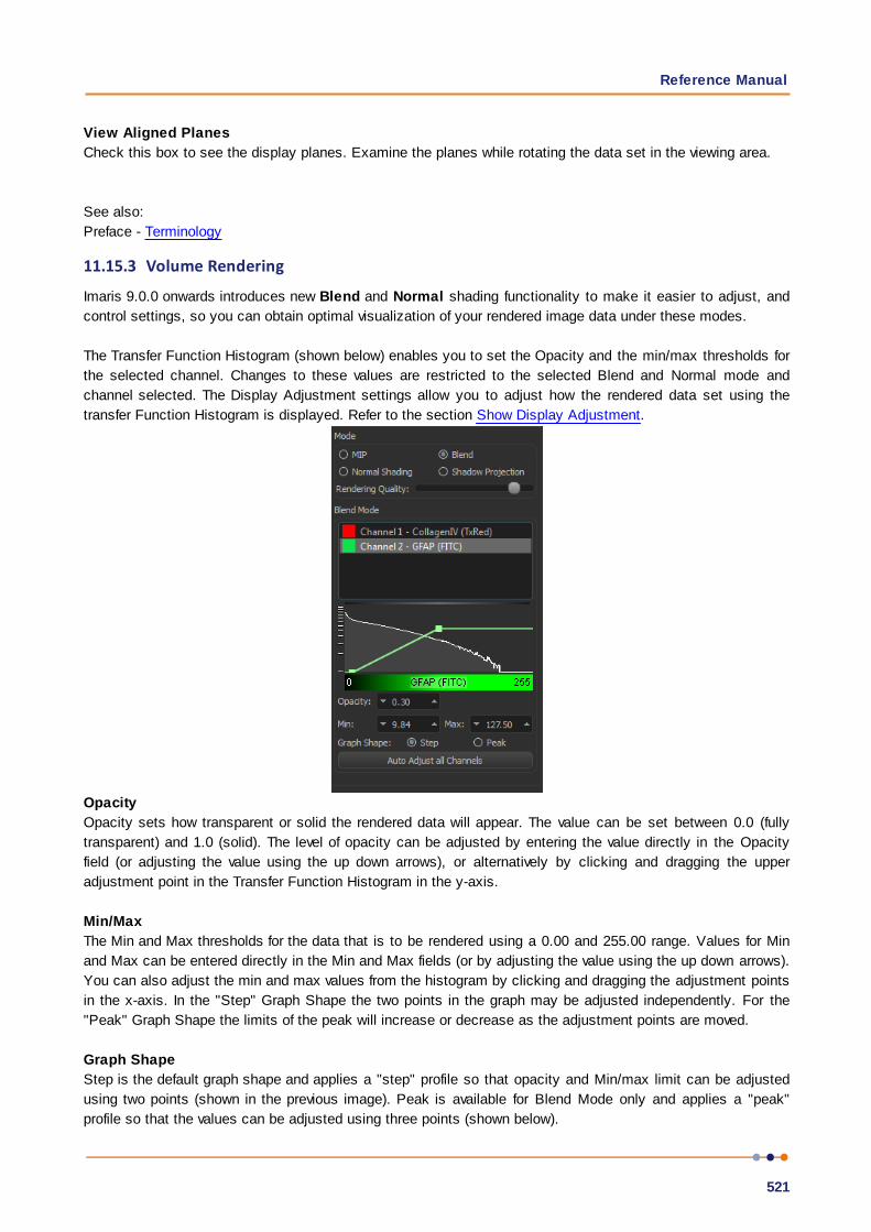
Reference Manual

521

View Aligned Planes

Check this box to see the display planes. Examine the planes while rotating the data set in the viewing area.

See also:

Preface - Terminology

11.15.3 Volume Rendering

Imaris 9.0.0 onwards introduces new Blend and Normal shading functionality to make it easier to adjust, and

control settings, so you can obtain optimal visualization of your rendered image data under these modes.

The Transfer Function Histogram (shown below) enables you to set the Opacity and the min/max thresholds for

the selected channel. Changes to these values are restricted to the selected Blend and Normal mode and

channel selected. The Display Adjustment settings allow you to adjust how the rendered data set using the

transfer Function Histogram is displayed. Refer to the section Show Display Adjustment.

Opacity

Opacity sets how transparent or solid the rendered data will appear. The value can be set between 0.0 (fully

transparent) and 1.0 (solid). The level of opacity can be adjusted by entering the value directly in the Opacity

field (or adjusting the value using the up down arrows), or alternatively by clicking and dragging the upper

adjustment point in the Transfer Function Histogram in the y-axis.

Min/Max

The Min and Max thresholds for the data that is to be rendered using a 0.00 and 255.00 range. Values for Min

and Max can be entered directly in the Min and Max fields (or by adjusting the value using the up down arrows).

You can also adjust the min and max values from the histogram by clicking and dragging the adjustment points

in the x-axis. In the "Step" Graph Shape the two points in the graph may be adjusted independently. For the

"Peak" Graph Shape the limits of the peak will increase or decrease as the adjustment points are moved.

Graph Shape

Step is the default graph shape and applies a "step" profile so that opacity and Min/max limit can be adjusted

using two points (shown in the previous image). Peak is available for Blend Mode only and applies a "peak"

profile so that the values can be adjusted using three points (shown below).

IMARIS

522

Auto Adjust all Channels Button

Use the AutoAdjust all Channels Button to automatically set all channels to calculated values.

Notes

Display Adjustment settings that map intensities to colors apply to all visualizations. Changing

them in MIP changes them for blend and normal shading as well (Control + D).

Zoom in/out on histogram using the mouse wheel

Double right click the histogram to reset zoom level to default

11.15.4 Tab Draw

Volume Painter

On the tab Draw you can find the settings for the Volume Painter. Use this Volume Painter to adjust the voxel

intensities before you do a segmentation based on Surfaces, Spots, or Filaments. (If an automatic algorithm is

not able to separate two objects, the intensity between these two objects can be "erased" in advance.) You can

draw disks, spheres, or hollow spheres into the selected image channel.

1. First select the desired channel and painter shape.

2. Rotate the view to execute a vertical cut.

3. Then customize the painter settings.

4. Change to the pointer mode Select.

5. Move the cursor to the desired position.

6. Hold down the Shift-key and click to add the shape.

7. In the viewing area you see a preview of the painter tool.

8. To re-edit a shape use the point selection.

9. Set intensity to 0 to erase a region, or set the intensity to 255 to fill a region.

10.To fix the shape click on the button Set Intensity.

Please note: The button Set Intensity changes the data set.

Selected Channel

Select the respective source channel.

Reference Manual

523

Painter Shape

Here you select the painter shape.

Disk

The painter is disk shaped. In the settings selection adjust the diameter, width and intensity of the disk (see

below).

Sphere

The painter is a sphere. In the settings selection adjust the diameter and intensity of the sphere (see below).

Hollow Sphere

The painter is a hollow sphere. In the settings selection adjust the diameter and intensity of the hollow sphere

(see below).

Selection

Diameter

Here you select the diameter of a disk, sphere, and hollow sphere. If your mouse has a wheel, you can use the

wheel to adjust the diameter.

Width

Here you select the width of a disk.

Intensity

Here you select the painter shape intensity. The shape preview in the viewing area changes accordingly. If you

want to cut parts out of the channel select 0 as intensity value.

Button Set Intensity

In the last step you click on this button to fix the shapes. The button Set Intensity changes the data set and it

is not possible to re-edit the shapes again.

Button Delete All

Click on this button to delete all inserted shapes in the preview.

Selected Point

You can use the following data fields and the button Delete to re-edit or delete a selected point.

Position [um] X, Y, Z

To select a point change to the pointer mode Select and click on a point. The color of the selected point

changes. The point position displays in the x, y, and z data field. To move the point click on the new position in

the viewing area or edit the x, y, or z data field.

Button Delete

Click on this button to delete the selected point.

IMARIS

524


Volume statistics are automatically computed. For the statistical variable values please refer to the Section

Menu Edit - Preferences... - Statistics - Volume. The Statistic tab collects and displays image statistical values

in Imaris. Statistic tab enable us to understand and compare different data sets through summarized statistical

values and graphical data presentations.

Several types of statistical tools enabling convenient organization and analysis of heterogeneous statistical

data. Statistical View is configured as follows:

a) Overall

b) Detailed

c) Selection

In a statistical data set the first column contains the name of the variable, followed by columns with calculated

statistical data. Corresponding statistical variable values are presented in rows.

To sort columns, click on the arrow in column heading. Click again to reverse the sort.

Overall Tab

Output of the Overall statistics provides an overview of the image single determining variables.


Button Settings - Configure List of visible statistics values.

Click on the button Settings and you switch to the window Preferences - Statistics - Volume.



Highlight the object in viewing area

Highlight the object on the Detailed Tab

Display of the values on the Selection Tab

Button Surfaces - Duplicate Selection to new Surfaces.


Surpass Tree.






automatically.


With a click on the button Export you open the Window Export Statistics. Select the file type (Comma

Separated Values *.csv, Excel file *.xls, or Excel XML *.xlm). If you select MS Excel, the program starts


See also:

Menu Edit - Preferences... - Statistics - Volume

Reference Manual

525

11.16 Export Selected Objects...In the Surpass Tree highlight all Items to be exported. To export all Surfaces, Contours, and External objects,

select the Export Selected Objects... .

Select menu Surpass - Export Selected Objects... .

The Save selection as External Objects box is displayed.

Select the directory and enter the name for the file to be saved and click OK. The object is saved as either as

an Inventor file with the extension *.iv, VRML2 file with extension *.vrml or WRL files with the extension .wrl.

The saved object can be loaded as External objects to another data set.

11.17 Delete Selected Objects ...In the Surpass Tree highlight all Items to be deleted. To delete all Surfaces, Spots, Contours, and External

objects, select the entire Scene folder.

Select menu Surpass - Delete Selected Objects.

The Delete selection window with a confirmation question is displayed.

11.18 Switch Pointer ModeIn the Surpass view there are two pointer modes: Select and Navigate.

Select

The cursor becomes an arrow. You use the pointer mode Select whenever you want to mark something in the

image, e.g. to set Measurement Points on the object surface.

Navigate

The cursor becomes two turning arrows. You use the pointer mode Navigate to move, rotate or zoom the image

in the viewing area.

Tip: You can easily switch between the two pointer modes using the ESC-Key. The effect is directly


11.19 InMotionThe function InMotion is a 3D viewing and precise interaction mode. Imaris produces a real 3D impression with

smooth animation of the image. This helps to get an understanding of the image depth, while manipulating with

Surpass objects: Spots, Filaments, Measurement Points.

How to Start the InMotion Mode?

Click on the icon in the Main toolbar.

Select View - InMotion.

To switch the mode off, click on the icon Surpass in the Main toolbar.

IMARIS

526

Adjust 3D Cursor Settings

To adjust the 3D cursor settings click on menu Edit - Preferences... - 3D Cursor.

11.20 Store Creation ParametersEnter a name for the Creation Parameter set. This name identifies the Creation Parameter item in the Arena

view and in the Creation Parameter list used in the Edit/Preference/Creation Parameters and would be used as

default name in the subsequent creation wizard algorithms.

Reference Manual

527

Section 12 Help

Quick Start Tutorials Ctrl + F1

Keyboard and Mouse F1

Reference Manual

Video Tutorials

Programming Interface

XTensionDocumentation

License... F2

Maintenance Plan

Check for Updates now... F3

Bitplane

About Imaris...

How to find the pdf based help for PC Users:

To open the pdf help file in Imaris first select Start- All Programs – Imaris.

The pdf version of the Reference Manual and Quick Start Tutorials are located there.

How to find the pdf based help for Mac Users:

To open the pdf help file in Imaris first locate and select the Imaris application file.

By default, the file is in the Application folder and the file name is Imaris 8.3.app.

With the right-click select the option Show Package Contents.

The new window will open.

Select the Contents folder and with a double-click select the Shared Support folder.

The pdf version of the Reference Manual and Quick Start Tutorials are located there.

See also:


12.1 Quick Start TutorialsThe Quick Start Tutorials provide you with the basic information on how-to-use Imaris but may also show yet

unrecognized new features of the software to the advanced user.

The tutorials are designed to be followed sequentially, but if you are already familiar with Imaris the basic

lessons may be skipped. The tutorials are cross-referenced by hyperlinks highlighted in blue underlined font.

The Table of Contents and the Index provide further support for navigation in the tutorials.

Each tutorial is a hands-on seminar, therefore it is recommended to move Imaris to the left hand side of the

screen and adjust the online tutorial on the right hand side of the screen and practice step-by-step.

12.2 Keyboard and MouseClick on this menu entry and the Reference Manual opens in the actual browser. The page for the global Mouse

& Keyboard functions displays.

Global Mouse & Keyboard Functions

For PC Users:

IMARIS

528


For Mac Users:


12.3 Reference ManualThe Reference Manual provides you with the information about Imaris: the menu(s), the different Imaris views

and the adjustable parameters in the program.

To find a specific parameter use the "Search function" in the online version of the Reference Manual.

Context Sensitive Help

For PC User:

With a right-click on a toolbar, a tab, or a parameter set the message Show Help... appears. With a left-click

on the message the Reference Manual opens in the actual browser and displays the corresponding page.

For Mac User:

With a Ctrl + click on a toolbar, a tab, or a parameter set the message Show Help... appears. With a click on

the message the Reference Manual opens in the actual browser and displays the corresponding page.

12.4 Video TutorialsThis link opens the Learning Center on the Bitplane website. Use the search facility to find the topics ofinterest.

12.5 Programming InterfaceSelect this to open the Imaris XT programming Interface.

12.6 XTension DocumentationThis Section provides a link to descriptions of XTension documentation.

12.7 Imaris OpenIf your computer is connected to the Internet, Imaris can directly open the Imaris Open webpage (http://

open.bitplane.com/).

12.8 License...Overview

Node-locked License

Reference Manual

529

Node-locked licenses grant permission to run the licensed software on one computer (node) only. Node-locked

licenses are the easiest way to license the software. You can use Imaris Administrator to directly download a

node-locked license from the Bitplane server. If your computer is not connected to the Internet it is also

possible to download this license from another computer and then copy it to the target machine.

Floating License

Floating licenses grant permission to run the licensed software on several computers. One floating license can

activate only one instance of the program at any given time. Floating licenses require the installation of a

separate license server that runs on a Windows computer. The server installation requires more technical know

how.

The Imaris Administrator application easily let you enable a floating license.

Demo License

A Demo License is a time-limited (usually one month) license. It is not an official licensing scheme and

therefore can't be purchased. It's main purpose is for internal Testing and to grant customers with licensing

issues an easy and quick workaround so that their productivity can continue until the problem is solved. Simply

open Imaris Administrator application and open the Demo License you received from your local support

representative.

Evaluation License

Evaluation Licenses are temporary licenses allowing customers to explore all fascinating possibilities Imaris

offers before actually purchasing it. The license is only limited in time (10 days), but not in features. Additionally

an Evaluation License is issued per user.

To get an Evaluation License you will have to register yourself first at:


An automatic mail response should provide you with your personal RegistrationID and its corresponding

Passcode. These credentials can then be entered during the application's start up.


To get an Imaris Open Developer License you first have to register at:


After you entered your OrderID click on the Imaris Open button to activate the Developer License.


server. Upon success, the button will turn on .

RegistrationIDPlease enter your RegistrationID you received by mail first.

First-time Installation

If you have installed Imaris for the very first time, you have to set up a license before you can use Imaris.

A dialog window appears during the start up of the application.

The same dialog window appears if you have accidentally deleted the license .

You now have two options how to proceed:



IMARIS

530

• If you have a Node-locked or a Floating License you should use the Imaris Administrator application for the

further license setup. This is done by simply clicking on the “Start Imaris Administrator” button. Please note

that the Imaris Administrator application needs administrative privileges.

• If you want to evaluate Imaris first, please register yourself first at:


The automatic mail response contains your RegistrationID and Passcode.

To enable an Evaluation License enter these values in the corresponding fields and click on the “Use Evaluation

License” button.

Please note that a working internet connection is needed to start up Imaris in Evaluation mode.

Installation of additional Licenses

If you already have set up a license but you want to add other licenses as well, you can do this in the License

Preferences dialog.

Once more, you'll have the option either to start the Imaris Administrator application or to use an Evaluation

License in addition if you would like to try out a new feature before buying the license.


Here you can adjust the default license settings.

Imaris Administrator is an application designed to manage the licenses of various Bitplane applications. It

provides a simple interface to add or delete any licenses. When a license is added, the license file gets copied

to a system folder where it is secure from (accidental) manipulation by standard users. Although it is possible

for administrators to modify license files directly in this folder we strongly advise you not to do so. It is

recommended to use the Imaris Administrator application instead.

Imaris Administrator Button

This button starts the Imaris Administrator. This is a tool shipped with Imaris in order to add or modify licenses.

Unless you want to use an Evaluation license you need to use the Imaris Administrator to set up your licenses.


Any change of licenses will require Imaris to be re-started.

Except for the Evaluation License which is bound to a single user, all other licenses are bound to the whole

system. Therefore any license modifications need administrative privileges.

If you have access to an administrative system account, Imaris Administrator should just start normally.

Start Imaris Administrator Button

This button starts Imaris Administrator. This is a tool shipped with Imaris in order to add or modify licenses.

Unless you want to use an Evaluation license you need to use Imaris Administrator to set up your licenses.



Evaluation License

Use Evaluation License Button

After you entered your RegistrationID and Passcode you can click on this button to enable the Evaluation


Reference Manual

531

License. This action requires an internet connection because the licenses are downloaded directly from the

Bitplane server. Upon success, the light bulb will turn on.

You can also disable your Evaluation License by clicking again on this button and the light bulb will turn off.

This indicates you aren't using any Evaluation Licenses.


RegistrationIDPlease enter your RegistrationID you received by mail.

PasscodePlease enter your Passcode you received by mail.

Available Licenses

The table displays all existing Imaris licenses on the system and additional information for each feature:

Version


Type

Which type of licensing scheme is used. An overview is given at the very beginning of this page.

Status


Expiration


Expiration


License colors


– Green: License is valid.

– Yellow: License is valid, but all licenses are currently in use.

– Red: License has expired.

– No color: License is not available (e.g. this additional license feature hasn't been purchased).

You can select with which license(s) your Imaris should start per default. Any change will require a new start ofImaris.

Check/Uncheck All

Check this box to enable or disable all available Imaris licenses on the system.

Please note that the Feature “ImarisBase” can't be disabled because this would render Imaris unusable.

The default Imaris Administrator executable can be found here:

Windows 7, 8 and 10:

64-bit: C:\Program Files\Bitplane\Imaris 9.0\ImarisAdministrator.exe

Mac OS X:

/Applications/Imaris 9.0.app/Contents/MacOS/ImarisAdministrator

If you did not have set up a license yet (e.g. first-time usage) this window is empty. In that case, please use

IMARIS

532

the Add License Location button to add a new license location.

Add License Location Button

Use this button to add new licenses. A description is given in the Add License Section.

Delete License Location

If you click this button, the selected license location entry in the table underneath will be deleted. Before using

this button, please make sure you selected the right table entry. In case of a node-locked license you are

asked if you want to keep the license. It is recommended that you keep all license files.

License Location Table

This table lists all available license locations. Normally it would be just enough to have one license location

defined. But there exist also good reasons to use multiple locations.

For example you might have a floating license server with just some basic features enabled. Maybe later you

purchased some additional features in a node-locked licensing scheme. You can now just define both locations

and the licensed features are merged on your system automatically.

The table shows also some additional Information:

• Type: This is either a License Server (floating license scheme) or a License File (all other schemes)

• Number of valid / total Licenses: These numbers shows you how many different features your license

contains and it lets you easily verify that all licenses are still valid.

If you click on another table entry, the License table underneath gets updated and shows you detailed

information about all available features of the current selected license location.

Licenses Table

In this table you have a detailed overview of all licensed features of a license location. You can switch between

different license locations by selecting the corresponding entry in the License Location table.

Each feature provides some information :

Version, Type, Status, Expiration

The validity of a license is also indicated by different colors.

Finish Button

This button is only enabled if you added at least one license location. It is an indicator when all necessary

steps to set up a license are done. If all features in the above License table are highlighted in green (or only

some of them) you successfully managed to add a license. If you click the button, it just closes Imaris

Administrator and you can proceed using Imaris.

Add License Window

First, you have to select your licensing scheme:

Download Node-locked License:

If you decide to add a Node-locked License, it will check that your computer is connected to the internet. If the

connection can be established successfully, the Online-Licensing Wizard is shown; if not, you have the

possibility to download the license from another computer which is described in the Offline-Licensing Wizard.

Online-Licensing Wizard:

This wizard has three steps:

Reference Manual

533

1. Select the Network Interface

You need to select the network interface which is bound to the license. If your Host-ID is already known to our

server, the available product for installation will be shown in the table below.

2. Check your Order-ID for newly ordered Products:

If you have ordered new products, you have to enter the Order-ID in this step. Clicking on the “Check Order-ID”

button will add the products to the table below. Once you checked an Order-ID, it is bound to the currently

selected network interface.

If your Host-ID is already known to the system, the available products will be shown in the tables below and you

could skip that step.

3. Select the Licenses for Installation

In this step you just have to mark all products you want to install by checking them in the left table.

The right table is for your information only and shows all currently installed products.

When you click on the “OK” button, the license file is downloaded and the corresponding entry is added to the

License Location table.

Offline-Licensing Wizard:

If you are not connected to the Internet, this could be due to two reasons:

1. your computer is behind a web proxy server which omits a direct connection or

2. your PC may be unplugged from the internet .

Therefore you have the following choices:

A) Set up a Proxy Server

Enter your proxy server's name and its port and click on the Test Connection button. If the connection could

be established you are automatically redirected to the Online-Licensing Wizard described above.

If not, either the credentials you entered are not correct or the connection is cut at another place in the network.

In that case please contact your network administrator or Bitplane Support teams [email protected] or

[email protected]

If you want to delete a previously set up proxy server, just delete both fields and click on the button again.

The proxy server settings can also be altered in Imaris' system preferences dialog.

B) Download the Node-locked License from another Computer

You can download the license from another computer connected to the internet.

On that machine log on to http://www.bitplane.com/activation/acti_offline_ident.html

and enter the Host-ID you wish to bind to the license together with your Order-ID into the web form. The

download of the license should immediately start and you could transfer the file afterwards to the offline

computer (e.g. by using a USB stick).

This instructions can be saved in a file by clicking the Save Instructions... button.

When you have downloaded the license you can just open it with the Open License... button or enter its path

directly into the field on the left of the button.

When you click OK the license file is copied to the proper location.

Define Floating License Server:

In order to add a Floating License Server, just enter the server's name and its port to the corresponding fields

and click on the OK button. The default port is 2700.





IMARIS

534

Install License from Existing File:

If you received a Demo License from your local support representative or you need to add a license file directly

you can use this wizard. If you click on the Open License... button you can browse to the license you want to

add. You can also specify the license file to load by entering its path directly into the field left from the button. If

you click on the OK button, the license is copied to the right location and it's added to your License Location

table.

See also:

Menu Edit - Preferences... - Calculation

Menu Edit - Preferences... - Licenses

Menu Edit - Preferences... - Display

12.9 Maintenance PlanImaris Infinity

A message is shown when your Imaris Infinity is about to expire.

If your contract has lapsed, the message indicates when that occurred.

You can renew your software maintenance contract for one or more years at a time. During the validity period of

your Imaris Infinity contract, you may install all updates to the program, contact our team for technical support

as well as access a wide range of educational and training services/tools.

Click on the Contact Sales button to send an email requesting a renewal of your Imaris Infinity contract.

Click on the Remind me later button to be reminded again in seven days.

If you click No, Thanks button and later change your mind and do wish to be reminded, change the setting in

the the Preferences/Update dialog.

12.10 Check for Updates now ...If your computer is connected to the Internet, Imaris can directly check, if a software update is available.

If new updates are available, a list of the available software versions is shown.

For a detailed list of new features, improvements and fixed bugs, please refer to the release notes.

12.11 Bitplane AGIf your computer is connected to the Internet, Imaris can directly open the Bitplane AG homepage

(www.bitplane.com).

12.12 AboutThe Imaris start screen displays.

Reference Manual

535

Imaris

Version number and release date.

Copyright 1993-2018 Bitplane AG

All rights reserved

European Patent Registry No. 05009677.7

Patent Pending.

Using XML parser expat: Copyright

1998, 1999, 2000. Thai Open Source

Software Center Ltd and Clark Cooper

www.bitplane.com

http://www.bitplane.com

IMARIS

536

Section 13 Toolbars

In the standard Imaris view there are three different toolbars available. The Main Toolbar, the Status Bar and the

Time Bar.

See also:

Surpass View - Overview - Camera Toolbar

13.1 Main ToolbarPlease refer to Section:

Open Imaris Menu - Open

Save Imaris Menu- Save

Export Imaris Menu - Export

Annotation Imaris Menu - Annotation

The display modes Slice, Section, Gallery and Easy 3D are in one icon group. Click on the arrow to select the

respective mode.


Slice Slice

Section Selection

Gallery Gallery

Easy 3D Easy 3D

3D View 3D View

Coloc Coloc

Animation Animation

Snapshot Snapshot

Bitplane AG Menu Help - Bitplane AG

13.2 Status BarAt the bottom of the screen you find the Status Bar.

Zoom %

Imaris lets you enlarge or reduce the viewing size of your data set as is required with the Zoom function. You

can zoom from 10% to 1000%. To go to a predefined zoom level, click the percentage of enlargement or

reduction you want. To specify a custom level, just type a zoom value. At 100% zoom factor one pixel on

screen represents one voxel.

Mouse Clicks to Zoom

Reference Manual

537


Click with the middle mouse button on the image, hold down the middle mouse button, and drag the mouse

up or down.

Hold the Shift-key and click with the right mouse button on the image, and drag the mouse up or down.



Button Fit

Click on this button to pan the position to best fit in the window and adjust the zoom factor.

Button Reset

Click on this button to reset the image to the original position, center the image in the middle and set the


Button Full Screen

Click on this button to maximize the viewing area to full size of the monitor. To return to the standard window,

click on the button Full Screen in the lower left corner.

Button Navi

Click on this button to toggle the display of the Navigation window of the data set in the upper right corner of the

viewing area. If you move the data set, the overview updates in real-time. In the pointer mode Select you can

click & drag the Navigation window to another position in the viewing area. The Navigation window is placed to

the nearest corner.

Change Position of the Navigation Window

In the pointer mode Select you can click & drag the Navigation window to any desired corner.

Double-click onto the Navigation window in order to switch off the automatic "snap-to-corner-mode". You can

drag it to any desired location. Re-double-click onto the Navigation window to switch the automatic "snap-to-

corner-mode" on again.

Right-click into the Navigation window in order to pan to the clicked position (moves the small yellow

window).

In the Section the position of the Navigation window is fixed (lower right corner) and can not be moved.

13.3 Time BarIf a time series is loaded, a Time Bar displays at the bottom of the main window. It contains a slider showing all

Time Points in the series, and control buttons (described below).

The Time Bar is visible in the display modes Slice, Section, Gallery 3D Preview, and Surpass. It allows you to

view a particular Time Point or to automatically play 4D images. The views change when selecting a new Time

Point.

Play and Record Time Series

IMARIS

538

Reference Frame button

Sets the reference frame playmode. Refer to Reference Frame.

When using reference frames, coloured tick marks indicate where the reference frames are located in time as

shown below for frames 0, 3, 5, 8 and 10:

The color of the tick mark indicates if the Keyframe is a Translation (green) and/or Rotational (magenta)

Reference Frame. In the above example, the reference frame located at frame 3 is both translational and

rotational, frame 5 is rotational only.

Time Settings button

Click on the time settings button to open the time parameter settings.

Jump to previous event and Jump to next event buttons

Use these options to move between event increments in the playback e.g. frames.

Play button

Click on this button to play the time series. To pause the continuous display through all the Time Points in the

time series re-click on the button.

Record button

To record the time series as movie click on the record button. The Export Movie window is displayed (see

below).

Slider

To inspect any the Time Point in the time series manually navigate the slider as follows (be sure that the

Pointer is in the Select mode):

Drag the slider handle to the left or right.

Moving the slider to the left reduces the time point, moving it to the right increase time point.

Select the slider handle with a left mouse click and then use the Arrow-keys to the left/to the right on the

keyboard.

Select the slider handle with a left mouse click and then press the Home-key or the End-key to display the

first respectively last Time Point.

The respective Time Point number is displayed on the right hand side of the slider in the number field.

Window: Export Movie

File name

Enter a file name.

Reference Manual

539

Export type

Select the desired file type (TIFF series, or AVI).

Movie Settings

Compression Factor

Select a compression factor between 0 (High Quality) and 100 (Low Quality), the default setting is 5. Use the

slider to set the compression factor between 0 and 100. Moving the slider to the left reduces the compression

point, moving it to the right increase compression pint. A lower factor results in a lower compression and

therefore a better quality, but also in a larger movie file.

Frame Rate

Define how many frames are displayed per second.

Play Movie with default Media Player when finished

Check the box to play the movie with the default media player when finished.

See also:

Menu Edit - Preferences ... - Time (default parameter settings)

Surpass View - Overview - Camera Toolbar (Pointer Select)

IMARIS

540

Section 14 Addendum

In this addendum you find the Imaris global Mouse & Keyboard PC and Mouse & Keyboard Mac functions,

some tips and tricks on how to customize your Imaris Interface for your daily routine, and a Terminology table

with frequently used technical terms and specific image processing terms.

14.1 Mouse & Keyboard PCIn the following you find the global Mouse & Keyboard functions.


Ctrl + 1 Activates the Slice

Ctrl + 2 Activates the Section

Ctrl + 3 Activates the Gallery

Ctrl + 4 Activates the Easy 3D

Ctrl + 5 Activates the 3D view

Ctrl + 6 Activates the Key Frame Animation

Ctrl + 7 Activates the Coloc

Ctrl + A Centers the image to the window

Ctrl + B Adjusts zoom factor and pan position to best fit the image into the window

Ctrl + C Copies current view to the clipboard

Ctrl + D Shows the Display Adjustment window

Ctrl + E Saves Scene file

Ctrl + F Refreshes the textures of all views

Ctrl + I Allows to inspect and edit the image properties

Ctrl + L Opens Scene file

Ctrl + N Toggles display of Navigation window

Ctrl + O Opens existing file

Ctrl + P Allows to edit the settings of Imaris

Ctrl + Q Exits the application

Ctrl + R Discards all changes and opens the current data set again

Ctrl + S Saves the current data set

Ctrl + T Saves the current view as a *.tif file

Ctrl + W Crops X, Y, or Z

Ctrl + Z Revokes the last action

Ctrl + Shift + A Adds channels of another image

Ctrl + Shift + B Deletes selected channels

Ctrl + Shift + C Copies the Imaris version, date and build to the clipboard

Ctrl + Shift + I Open an additional image without closing the existing image.

Ctrl + Shift + P Allows to edit figures and annotations

F1 Opens Reference Manual

F2 Displays or updates the license status

F3 Automatic check for updates

F11 Maximizes the viewing area to the full size of your monitor

Reference Manual

541

Ctrl + F1 Opens Quick Start Tutorials

Alt + F4 Exits the application

Del Deletes selected objects

Right-click Opens Context Sensitive Help

Global Mouse & Keyboard Functions to Navigate in All Imaris Views


Move down: zoom in


Left-click & drag Rotate image

Context Specific Mouse & Keyboard Functions

In the varying Imaris views there are additional shortcuts, please refer to the respective Section in this

Reference Manual for details.

Menu Edit - Show Display Adjustments - Mouse & Keyboard PC

Slice - Mouse & Keyboard PC

Section - Mouse & Keyboard PC

Gallery - Mouse & Keyboard PC

Easy 3D - Mouse & Keyboard PC

3D View - Overview - Mouse & Keyboard PC

Clipping Plane - Mouse & Keyboard PC

Contour Surface -Shortcuts Overview

External Object - Mouse & Keyboard PC

Filament - Mouse & Keyboard PC

Light Source - Mouse & Keyboard PC

Measurement Point - Mouse & Keyboard PC

Oblique Slicer - Mouse & Keyboard PC

Ortho Slicer - Mouse & Keyboard PC

Surface-Shortcuts Overview

Spots - Mouse & Keyboard PC

Animation - Mouse & Keyboard PC

Coloc - Mouse & Keyboard PC


With a right-click on a toolbar, a tab, or a parameter set the message Show Help... appears. With a left-click

on the message the Reference Manual opens in the actual browser and displays the corresponding page.

14.2 Mouse & Keyboard MacIn the following you find the global Mouse & Keyboard functions.


Command + 1 Activates the Slice

Command + 2 Activates the Section

IMARIS

542

Command + 3 Activates the Gallery

Command + 4 Activates the Easy 3D

Command + 5 Activates the 3D View

Command + 6 Activates the Key Frame Animation

Command + 7 Activates the Coloc

Command + A Centers the image to the window

Command + B Adjusts zoom factor and pan position to best fit the image into the

window

Command + C Copies current view to the clipboard

Command + D Shows the Display Adjustment window

Command + E Saves Scene file

Command + F Refreshes the textures of all views

Command + I Allows to inspect and edit the image properties

Command + L Opens Scene file

Command + N Toggles display of Navigation window

Command + O Opens existing file

Command + , Allows to edit the settings of Imaris

Command + Q Exits the application

Command + R Discards all changes and opens the current data set again

Command + S Saves the current data set

Command + T Saves the current view as a *.tif file

Command + W Crops X, Y, or Z

Command + Z Revokes the last action

Command + Shift + A Adds channels of another image

Command + Shift + B Deletes selected channels

Command + Shift + C Copies the Imaris version, date and build to the clipboard

Command + Shift + P Allows to edit figures and annotations

Ctrl + Shift + I Open an additional image without closing the existing image.

F1 Opens Reference Manual

F2 Displays or updates the license status

F3 Automatic check for updates

Command + F11 Maximizes the viewing area to the full size of your monitor

Command + F1 Opens Quick Start Tutorials

Del Deletes selected objects

Ctrl-click Opens Context Sensitive Help

Global Mouse & Keyboard Functions to Navigate in All Imaris Views



Move down: zoom in



Reference Manual

543









Move down: zoom in


Context Specific Mouse & Keyboard Functions

In the varying Imaris views there are additional shortcuts, please refer to the respective Section in this

Reference Manual for details.

Edit - Show Display Adjustments - Mouse & Keyboard Mac

Slice - Mouse & Keyboard Mac

Section - Mouse & Keyboard Mac

Gallery - Mouse & Keyboard Mac

Easy 3D - Mouse & Keyboard Mac

3D View - Overview - Mouse & Keyboard Mac

Clipping Plane - Mouse & Keyboard Mac

Contour Surface - Shortcuts Overview

External Object - Mouse & Keyboard Mac

Filament - Mouse & Keyboard Mac

Light Source - Mouse & Keyboard Mac

Measurement Point - Mouse & Keyboard Mac

Oblique Slicer - Mouse & Keyboard Mac

Ortho Slicer - Mouse & Keyboard Mac

Surface-Shortcuts Overview

Spots - Mouse & Keyboard Mac

Animation - Mouse & Keyboard Mac

Coloc - Mouse & Keyboard Mac


With a Ctrl + click on a toolbar, a tab, or a parameter set the message Show Help... appears. With a click on

the message the Reference Manual opens in the actual browser and displays the corresponding page.

14.3 Customize InterfaceIn this Section you find a collection of tips and tricks to customize the Imaris interface for your daily routine.

Histogram

Logarithmic or linear histogram display.

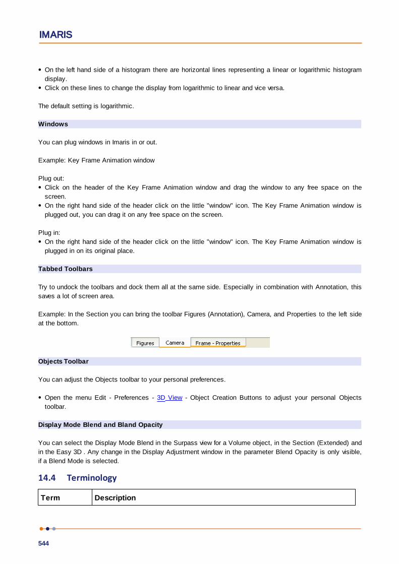
IMARIS

544

On the left hand side of a histogram there are horizontal lines representing a linear or logarithmic histogram

display.

Click on these lines to change the display from logarithmic to linear and vice versa.

The default setting is logarithmic.

Windows

You can plug windows in Imaris in or out.

Example: Key Frame Animation window

Plug out:

Click on the header of the Key Frame Animation window and drag the window to any free space on the

screen.

On the right hand side of the header click on the little "window" icon. The Key Frame Animation window is

plugged out, you can drag it on any free space on the screen.

Plug in:

On the right hand side of the header click on the little "window" icon. The Key Frame Animation window is

plugged in on its original place.

Tabbed Toolbars

Try to undock the toolbars and dock them all at the same side. Especially in combination with Annotation, this

saves a lot of screen area.

Example: In the Section you can bring the toolbar Figures (Annotation), Camera, and Properties to the left side

at the bottom.

Objects Toolbar

You can adjust the Objects toolbar to your personal preferences.

Open the menu Edit - Preferences - 3D View - Object Creation Buttons to adjust your personal Objects

toolbar.

Display Mode Blend and Bland Opacity

You can select the Display Mode Blend in the Surpass view for a Volume object, in the Section (Extended) and

in the Easy 3D . Any change in the Display Adjustment window in the parameter Blend Opacity is only visible,

if a Blend Mode is selected.

14.4 Terminology

Term Description

Reference Manual

545

Channel A channel is a particular piece of information that has been recorded for all voxels. Mostof the time in light microscopy, the different channels are intensities that have beenmeasured at different wavelengths. For instance, a two-channel data set contains twointensities for each voxel, one intensity measured in channel 1 (e.g., green light) and oneintensity in channel 2 (e.g., red light). Ideally, the intensity values present in differentchannels are independent of one another.

Coordinates Any position in the data set can be described either in the voxel grid (e.g., voxel no. 5 inx-direction) or by a coordinate, which corresponds to a m). The distance relative to adefined origin in the real world (e.g. 2 latter) requires the correct calibration of the dataset, i.e. that the voxel size is defined appropriately. Generally, in Imaris the origin of thedata set is in the left bottom corner. If the data set was cropped from a larger data set,the bottom left corner may have minimum coordinates that are not equal to (0,0,0).

Image stack A 3D data set is sometimes called an image stack consisting of 2D images stacked oneach other.

MIP A maximum intensity projection (MIP) is a computer visualization method for 3D datathat projects in the visualization plane the voxels with maximum intensity that fall in theway of parallel rays traced from the viewpoint to the plane of projection.

Original Data Set

A 3D data set that cannot be derived from any other data set using Bitplane software.Usually "Original data sets" have been acquired using an image sensor and are loadedinto Imaris.

Rendering A technique that visualizes a multi-dimensional data set as a two-dimensional image thatcan be displayed on a computer screen or printed on a laser printer.

ResultantImage

An image that has been computed using Imaris.

Standard

Deviation

In probability and statistics, the standard deviation of a probability distribution, randomvariable, or population or multiset of values is a measure of the spread of its values. It isdefined as the square root of the variance.

The standard deviation is the root mean square (RMS) deviation of values from theirarithmetic mean. For example, in the population {4, 8}, the mean is 6 and the standarddeviation is 2. This may be written: {4, 8} 6. In this case 100% of the values in thepopulation are at one standard deviation of the mean.

The standard deviation is the most common measure of statistical dispersion, measuringhow widely spread the values in a data set are. If the data points are close to the mean,then the standard deviation is small. Conversely, if many data points are far from themean, then the standard deviation is large. If all the data values are equal, then thestandard deviation is zero.

The standard deviation (s) of a population can be estimated by a modified standarddeviation (s) of a sample.

Threshold A threshold in Imaris is a gray value, which acts as a limit. All gray values above (orbelow) are assigned a particular functionality.

Time Point A time point is a single 3D image containing one or many channels. The term is usedregardless of what data is actually stored in the channels. In particular, the channelscould contain data taken at different points in time with a changing object.

IMARIS

546

VolumeRendering

A rendering technique which operates directly on the voxel data. The input imageconsisting of a collection of voxels arranged in a regular grid is converted directly into the2D output image.

Voxels A volume data set is composed of volume elements called voxels. The voxels are thesmallest units within the image about which we have distinct information in the form of ameasured intensity. The dimensions of an individual voxel are specified in most image fileformats supported by Imaris.

Documents

Imaris Reference Manual - Queensland Brain Institute · The Arena view consists of a number of elements. The search field is at the top left of the Arena view. Below the search field