Embed Size (px)
Citation preview
Proceedings, Thirtieth Workshop on Geothermal Reservoir Engineering Stanford University, Stanford, California, January 31-February 2, 2005 SGP-TR-176
IMAGING GEOTHERMAL FRACTURES BY CSAMT METHOD AT TAKIGAMI AREA IN JAPAN
Koichi Tagomori*, Enjang Mustopa, Hisashi Jotaki, Hideki Mizunaga and Keisuke Ushijima
*West Japan Engineering Co. Watanabe-Dori 2-1-82, Fukuoka 810-0004, Japan
ABSTRACT
Controlled Source Audio-frequency Magneto-Telluric (CSAMT) survey was carried out in Takigami geothermal field. Stations were taken closely with regular grid spacing of 150 m. The purpose of the measurements is to delineate a detailed resistivity structure and location of electrical discontinuities that may reflect a possible faults and fractures correlated with a promising reservoir. Although the CSAMT measurements were conducted at a distance of 6 km away from a transmitter, the CSAMT data still contain some near field data when the frequency from transmitter signal is low range. Therefore, before applying two-dimensional (2-D) magnetotelluric (MT) inversion analysis of transverse magnetic (TM) mode, data corrections for a near field and transition zone were made. The interpretation results based on 2-D inversion show that there are some electrical discontinuities are found in the N-S and W-E directions, which correlate with the trend of some faults where the geothermal reservoir may exist. The electrical discontinuity Fd in N-S direction correlates with the Noine fault zone, which divides the subsurface into eastern and western parts according to the characteristics of electrical resistivity, permeability, temperature, and reservoir depth. The electrical discontinuity Fa in W-E direction corresponds to the Teradoko fault where the major production wells have been drilled in the area.
INTRODUCTION
Signal of magnetotelluric (MT) method is considered to be due to thunderstorms and solar winds in ionosphere for which the field strength and polarization vary with time of day and season. To improve the signal strength problem of the MT method, Goldstein and Strangway (1975) developed the audiofrequency MT technique with a grounded electric dipole as an artificial source called controlled-source audiofrequency magnetotelluric (CSAMT). Over the years, CSAMT has emerged as a powerful exploration tool and has found its application in a mineral exploration (Zonge, et.al.,1986), geothermal investigation (Sandberg, 1982, Bartel 1987) and a potential radioactive waste disposal characterization (Unsworth, 2000). An excellent review of CSAMT and its application is given by Zonge and Hughes (1981). The advantages of this technique operated with MT method are that the polarization of the fields can be selected by the orientation of the transmitting antenna and the signal strengths do not depend on the time of day or season. However in the CSAMT method, the non-plane wave nature of the source limits the interpretation of the data. Recognizing this, the CSAMT measurement must be carried out at a distance greater than 3-5 skin depths from the transmitter site where the plane wave approximation is valid. Mustopa et al.(2001) have interpreted the MT data in the Takigami geothermal field to determine the subsurface resistivity structure correlated to the promising reservoir zone and distribution of fault systems and trends. However,
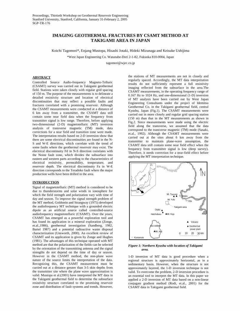
the stations of MT measurements are not in closely and regularly spaced. Accordingly, the MT data interpretation results do not sufficiently represent a full resistivity imaging reflected from the subsurface in the area.The CSAMT measurements, in the operating frequency range of 0.167 Hz to 1024 Hz, and one-dimensional (1-D) inversion of MT analysis have been carried out by West Japan Engineering Consultants under the project of Idemitsu Geothermal Co. in the Takigami geothermal field, central Kyushu, Japan (Fig.1). The CSAMT measurements were carried out in more closely and regular grid spacing station (150 m) than that in the MT measurements as shown in Fig.2. Since measurements were made using the electric field along the transverse, we assumed that the data correspond to the transverse magnetic (TM) mode (Sasaki, et.al., 1992). Although the CSAMT measurements were carried out at the sites about 6 km away from the transmitter to maintain plane-wave assumption, the CSAMT data still contain some near field effect when the frequency from transmitter signal is low (deep survey). Therefore, it needs correction for a near-field effect before applying the MT interpretation technique.
Japa
n Sea
Kyushu
Aso caldera
Mt. Aso
Mt. Kuju
Otake
Hatchobaru
Mt. Tsurumi
Mt. Yufu
Takigami area
Beppu
Oita
Volcano
Geothermal power plant
0 10 20 30 km
Kumamoto
Figure 1: Northern Kyushu with location of Takigami area.
1-D inversion of MT data is good procedure when a regional structure is approximately horizontal, as in a sedimentary basin. However, when the structure is not approximately layered, the 1-D inversion technique is not valid. To overcome the problem, 2-D inversion procedure is an essential tool to interpret the MT data. In this paper we applied a 2-D inversion of MT data based on a non-linear conjugate gradient method (Rodi, et.al., 2001) for the CSAMT data in Takigami geothermal field.
A B C D E F G H I J K L M NYufuin Machi
778
698
Nogam
igawa
711
869
Tateishilake
Yamashita lake
926
800
850
974
750
850
1024
945
1000
1575
1425
1275
1125
975
825
675
525
375
225
75
1575
1425
1275
1125
975
825
675
525
375
225
75
1575
1425
1275
1125
975
825
675
525
375
225
75
1575
1425
1275
1125
975
825
675
525
375
225
75
1575
1425
1275
1125
975
825
675
525
375
225
75
1575
1425
1275
1125
975
825
675
525
375
225
75
1575
1425
1275
1125
975
825
675
525
375
225
75
1575
1425
1275
1125
975
825
675
525
375
225
75
1575
1425
1275
1125
975
825
675
525
375
225
75
1575
1425
1275
1125
975
825
675
525
375
225
75
1575
1425
1275
1125
975
825
675
525
375
225
75
1575
1425
1275
1125
975
825
675
525
375
225
75
1575
1425
1275
1125
975
825
675
525
375
225
75
1575
1425
1275
1125
975
825
675
525
375
225
75
Legend
0 100 200 300 400 500 600 700 800
1 : 10.000
: Sounding station
: Well head
NE4
TT-16
NE2
TT-20
TT-16SNE5
TT-7
NE-11R
TT-17STT-17
TT-14R
TT-14
NE10
TT-13
TT-13S
N3-MW-5
Tateishi lake
Yamashita lake
Nogam
i gawaField survey
area
Current source
Figure 2: The location map of CSAMT measurements in Takigami area.
GEOLOGICAL SETTING
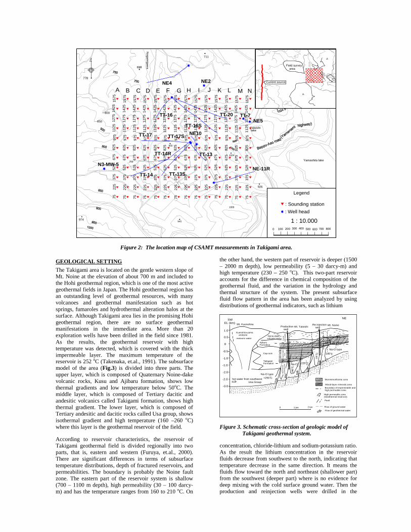
The Takigami area is located on the gentle western slope of Mt. Noine at the elevation of about 700 m and included to the Hohi geothermal region, which is one of the most active geothermal fields in Japan. The Hohi geothermal region has an outstanding level of geothermal resources, with many volcanoes and geothermal manifestation such as hot springs, fumaroles and hydrothermal alteration halos at the surface. Although Takigami area lies in the promising Hohi geothermal region, there are no surface geothermal manifestations in the immediate area. More than 20 exploration wells have been drilled in the field since 1981. As the results, the geothermal reservoir with high temperature was detected, which is covered with the thick impermeable layer. The maximum temperature of the reservoir is 252 oC (Takenaka, et.al., 1991). The subsurface model of the area (Fig.3) is divided into three parts. The upper layer, which is composed of Quaternary Noine-dake volcanic rocks, Kusu and Ajibaru formation, shows low thermal gradients and low temperature below 50oC. The middle layer, which is composed of Tertiary dacitic and andesitic volcanics called Takigami formation, shows high thermal gradient. The lower layer, which is composed of Tertiary andesitic and dacitic rocks called Usa group, shows isothermal gradient and high temperature (160 –260 oC) where this layer is the geothermal reservoir of the field.
According to reservoir characteristics, the reservoir of Takigami geothermal field is divided regionally into two parts, that is, eastern and western (Furuya, et.al., 2000). There are significant differences in terms of subsurface temperature distributions, depth of fractured reservoirs, and permeabilities. The boundary is probably the Noine fault zone. The eastern part of the reservoir system is shallow (700 – 1100 m depth), high permeability (30 – 100 darcy-m) and has the temperature ranges from 160 to 210 oC. On
the other hand, the western part of reservoir is deeper (1500 – 2000 m depth), low permeability (5 – 30 darcy-m) and high temperature (230 – 250 oC). This two-part reservoir accounts for the difference in chemical composition of the geothermal fluid, and the variation in the hydrology and thermal structure of the system. The present subsurface fluid flow pattern in the area has been analyzed by using distributions of geothermal indicators, such as lithium
Monmtmorillonite zone
2 km1 km0
Mixed-layer minerals zone
Boundary of impermeable andhigh permeable zone
High permeable zone(Geothermal reservoir)
Fault
Flow of ground water
Flow of geothermal water
SWEL (km)
1.0
0.5
0
-0.5
-1.0
-1.0
-2.0
-2.0
-3.0
Kuenohira-yama andesite
meteoric water
hot water from southwestUsa Group
Na-Cl type
>250
Na-ClTakigamiFormation
0C
type
Na-Cl type
180 0C
220 0C
Production well
Mt. TateishiRe-injection well
Mt. Noine
NE
Mt. Kuenohira
Noine-dakevolcanic rocks
AjibaruFormation
Cap rock
Impe
rmea
ble
z
one
Hyd
roth
erm
alco
nvec
tive
zone
G
roun
dw
ater
aqu
ifer
200
0 C
0 C24
0
Figure 3. Schematic cross-section al geologic model of Takigami geothermal system.
concentration, chloride-lithium and sodium-potassium ratio. As the result the lithium concentration in the reservoir fluids decrease from southwest to the north, indicating that temperature decrease in the same direction. It means the fluids flow toward the north and northeast (shallower part) from the southwest (deeper part) where is no evidence for deep mixing with the cold surface ground water. Then the production and reinjection wells were drilled in the
southwestern and the northeastern part, respectively. The most adequate capacity (about 70 % of steam) of the production was estimated at 55 MW of power generation (Furuya, 1988).
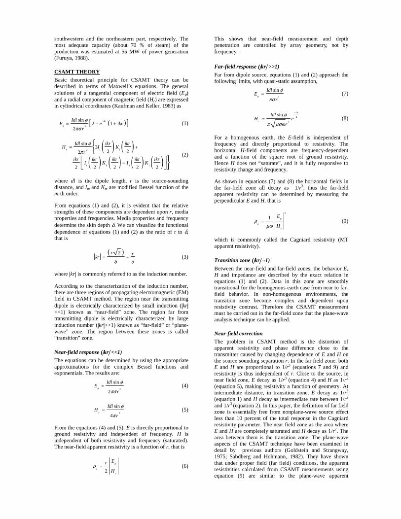
CSAMT THEORY
Basic theoretical principle for CSAMT theory can be described in terms of Maxwell’s equations. The general solutions of a tangential component of electric field (Eφ) and a radial component of magnetic field (Hr) are expressed in cylindrical coordinates (Kaufman and Keller, 1983) as
( )[ ]3
sin2 1
2
ikrIdlE e ikr
rφ
φ
πσ
−= − + (1)
( ) ( ){( ) ( ) ( ) ( ) }
2 1 1
1 0 0 1
sin3
2 22
2 2 2 2 2
r
Idl ikr ikrH I K
r
ikr ikr ikr ikr ikrI K I K
φ
π= +
−⎡ ⎤⎣ ⎦
(2)
where dl is the dipole length, r is the source-sounding distance, and Im and Km are modified Bessel function of the m-th order.
From equations (1) and (2), it is evident that the relative strengths of these components are dependent upon r, media properties and frequencies. Media properties and frequency determine the skin depth δ. We can visualize the functional dependence of equations (1) and (2) as the ratio of r to δ, that is
( )2r rkr
δ δ= ≈ (3)
where |kr| is commonly referred to as the induction number.
According to the characterization of the induction number, there are three regions of propagating electromagnetic (EM) field in CSAMT method. The region near the transmitting dipole is electrically characterized by small induction (|kr| <<1) known as “near-field” zone. The region far from transmitting dipole is electrically characterized by large induction number (|kr|>>1) known as “far-field” or “plane-wave” zone. The region between these zones is called “transition” zone.
Near-field response (|kr| <<1)
The equations can be determined by using the appropriate approximations for the complex Bessel functions and exponentials. The results are:
3
sin
2
IdlE
rφ
φ
πσ≈ (4)
2
sin
4r
IdlH
r
φ
π≈ (5)
From the equations (4) and (5), E is directly proportional to ground resistivity and independent of frequency. H is independent of both resistivity and frequency (saturated). The near-field apparent resistivity is a function of r, that is
2a
r
Er
H
φρ ≈ (6)
This shows that near-field measurement and depth penetration are controlled by array geometry, not by frequency.
Far-field response (|kr| >>1)
Far from dipole source, equations (1) and (2) approach the following limits, with quasi-static assumption,
3
sinIdlE
rφ
φ
πσ≈ (7)
4
3
sini
r
IdlH e
r
πφ
π µσω
−
≈ (8)
For a homogenous earth, the E-field is independent of frequency and directly proportional to resistivity. The horizontal H-field components are frequency-dependent and a function of the square root of ground resistivity. Hence H does not “saturate”, and it is fully responsive to resistivity change and frequency.
As shown in equations (7) and (8) the horizontal fields in the far-field zone all decay as 1/r3, thus the far-field apparent resistivity can be determined by measuring the perpendicular E and H, that is
2
1a
r
E
H
φρµω
= (9)
which is commonly called the Cagniard resistivity (MT apparent resistivity).
Transition zone (|kr| ≈1)
Between the near-field and far-field zones, the behavior E, H and impedance are described by the exact relation in equations (1) and (2). Data in this zone are smoothly transitional for the homogenous-earth case from near to far-field behavior. In non-homogenous environments, the transition zone become complex and dependent upon resistivity contrast. Therefore the CSAMT measurement must be carried out in the far-field zone that the plane-wave analysis technique can be applied.
Near-field correction
The problem in CSAMT method is the distortion of apparent resistivity and phase difference close to the transmitter caused by changing dependence of E and H on the source sounding separation r. In the far field zone, both E and H are proportional to 1/r3 (equations 7 and 9) and resistivity is thus independent of r. Close to the source, in near field zone, E decay as 1/r3 (equation 4) and H as 1/r2 (equation 5), making resistivity a function of geometry. At intermediate distance, in transition zone, E decay as 1/r3 (equation 1) and H decay as intermediate rate between 1/r2 and 1/r3 (equation 2). In this paper, the definition of far field zone is essentially free from nonplane-wave source effect less than 10 percent of the total response in the Cagniard resistivity parameter. The near field zone as the area where E and H are completely saturated and H decay as 1/r2. The area between them is the transition zone. The plane-wave aspects of the CSAMT technique have been examined in detail by previous authors (Goldstein and Strangway, 1975; Sabdberg and Hohmann, 1982). They have shown that under proper field (far field) conditions, the apparent resistivities calculated from CSAMT measurements using equation (9) are similar to the plane-wave apparent
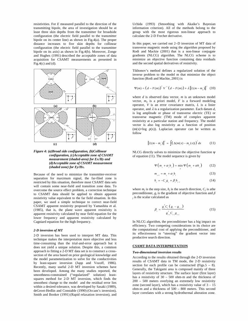
resistivities. For E measured parallel to the direction of the transmitting bipole, the area of investigation should be at least three skin depths from the transmitter for broadside configuration (the electric field parallel to the transmitter bipole on its center line) as shown in Fig.4(a). The proper distance increases to five skin depths for collinear configuration (the electric field parallel to the transmitter bipole on its axis) as shown in Fig.4(b). Moreover, Zonge and Hughes (1991) described the acceptable zones of data acquisition for CSAMT measurements as presented in Fig.4(c) and (d).
3
3
- 45
45
Z X
Ex
Z X
55
- 30
30
Ex
(a) (b)
Z X
3
5
3
5
- 45 - 30
30
45
3
- 5
5
8595
3
Z X
(c) (d)
Figure 4: (a)Broad side configuration, (b)Collinear configuration, (c)Acceptable zone of CSAMT measurement (shaded-area) for Ex/Hy and (d)Acceptable zone of CSAMT measurement (shaded zone) for Ey/Hx.
Because of the need to minimize the transmitter-receiver separation for maximum signal, the far-filed zone is restricted by this situation, therefore most CSAMT data sets will contain some near-field and transition zone data. To overcome the source effect problem, a correction technique to CSAMT data should be applied to obtain apparent resistivity value equivalent to the far field situation. In this paper, we used a simple technique to correct near-field CSAMT apparent resistivity proposed by Yamashita et al. (1985), that is, the plane wave apparent resistivity is apparent resistivity calculated by near field equation for the lower frequency and apparent resistivity calculated by Cagniard equation for the high frequency.
2-D inversion of MT
2-D inversion has been used to interpret MT data. This technique makes the interpretation more objective and less time-consuming than the trial-and-error approach but it does not yield a unique solution. Despite this, a common approach to fitting a 2-D MT data set is to construct a cross-section of the area based on prior geological knowledge and the model parameterization to solve for the conductivities by least-square inversion (Jupp and Vozoff, 1986). Recently, many useful 2-D MT inversion schemes have been developed. Among the many studies reported, the smoothness-constrained (“regularized” solution) least-squares method for 2-D MT inversion, which finds the smoothest change to the model and the residual error lies within a desired tolerance, was developed by Sasaki (1989), deGroot-Hedlin and Constable (1990) (Occam’s inversion), Smith and Booker (1991) (Rapid relaxation inversion), and
Uchida (1993) (Smoothing with Akaike’s Bayesian information criterion). All of the methods belong to the group with the most rigorous non-linear approach to calculate the 2-D Frechet derivative.
In this paper, we carried out 2−D inversion of MT data of transverse magnetic mode using the algorithm proposed by Rodi and Mackie (2001) that is a non-linear conjugate gradients (NLCG) algorithm. The NLCG scheme is to minimize an objective function containing data residuals and the second spatial derivatives of resistivity.
Tikhonov’s method defines a regularized solution of the inverse problem to the model m that minimize the object function (Rodi and Machie, 2001) is
( ) ( ) 21
0( ) ( ) ( ) ( )
T
m d F m V d F m L m mλ−Ψ = − − + − (10)
where d is observed data vector, m is an unknown model vector, mo is a priori model, F is a forward modeling operator, V is an error covariance matrix, L is a linier operator, and λ is a regularization parameter. Each datum di is log amplitude or phase of transverse electric (TE) or transverse magnetic (TM) mode of complex apparent resistivity at a particular station and frequency. The model vector is also log resistivity as a function of position (m(x)=log ρ(x)). Laplacian operator can be written as follow
( )22
0( ) ( ( ) ( ))
oL m m m x m x dx− = ∆ −∫ (11)
NLCG directly solves to minimize the objective function ψ of equation (11). The model sequence is given by
( ) ( )minj j j j j
m h m hα
α αΨ + = Ψ + (12)
1j j j jm m hα
+= + (13)
1j j j j jh C g hβ
−= − + (14)
where mj is the step size, hj is the search direction, Cj is athe preconditioner, gj is the gradient of objective function and βj is the scalar calculated as
( )1
1 1 1
T
l l l l
j T
l l l
g C g g
g C gβ −
− − −
−= (15)
In NLCG algorithm, the preconditioner has a big impact on efficiency. Two competing considerations in its choice are the computational cost of applying the preconditioner, and its effectiveness in “steering” the gradient vector into productive search direction.
CSAMT DATA INTERPRETATION
Two-dimensional inversion results
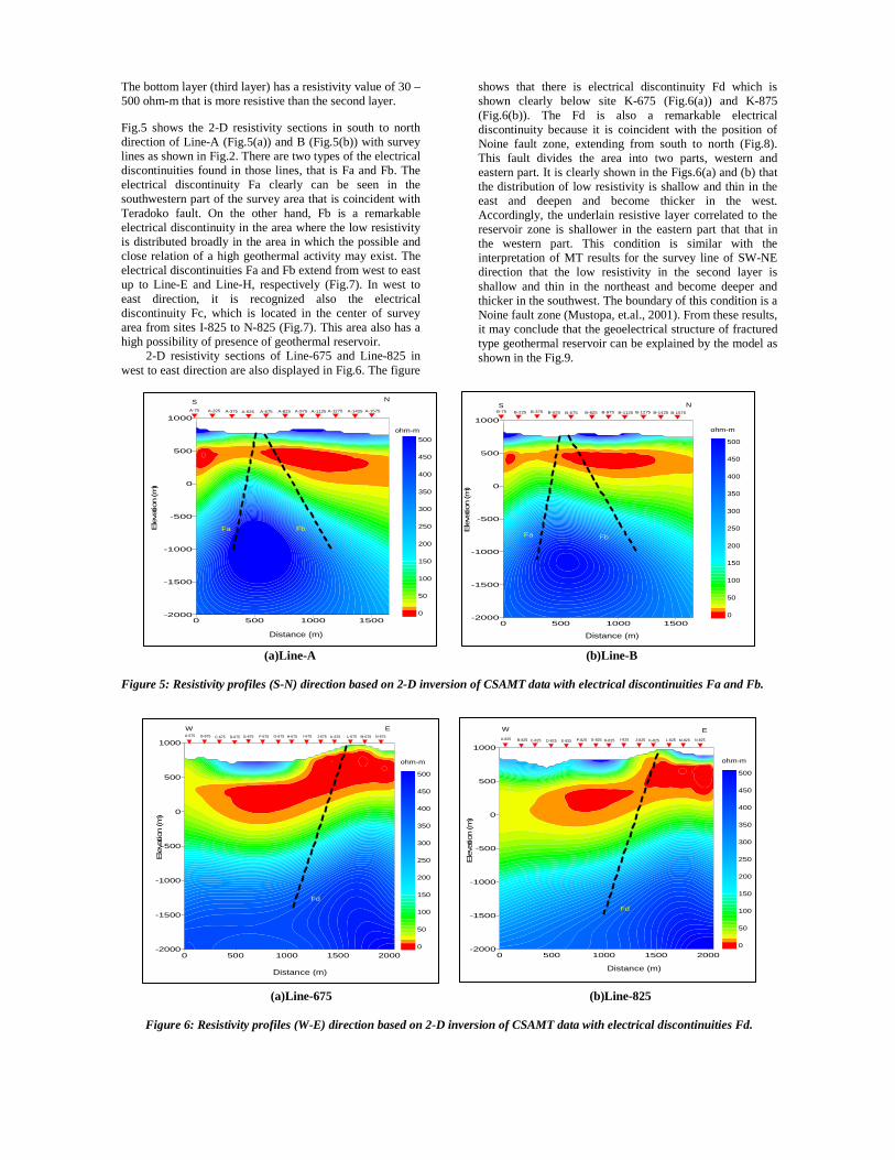
According to the results obtained through the 2-D inversion results of CSAMT data in TM mode, the 2-D resistivity section for each profile can be constructed (Figs.5 – 8). Generally, the Takigami area is composed mainly of three layers of resistivity structure. The surface layer (first layer) has a resistivity of 30 – 500 ohm-m and the thickness of 200 – 500 meters overlying an extremely low resistivity zone (second layer), which has a resistivity value of 3 – 15 ohm-m and a thickness of 500 – 800 meters. This second layer correlates with a strong hydrothermal alteration zone.
Ele
vatio
n (m
)
0
50
100
150
200
250
300
350
400
450
500
ohm-m
0 500 1000 1500-2000
-1500
-1000
-500
0
500
1000B-225 B-375 B-525 B-675 B-825 B-975 B-1125 B-1275 B-1425 B-1575B-75
Fa
S N
Distance (m)
Fb
0 500 1000 1500-2000
-1500
-1000
-500
0
500
1000A-225 A-375 A-525 A-675 A-825 A-975 A-1125 A-1275 A-1425 A-1575A-75
0
50
100
150
200
250
300
350
400
450
500
ohm-m
Fa
S N
Distance (m)
Ele
vatio
n (m
)
Fb
0
50
100
150
200
250
300
350
400
450
500
ohm-m
0 500 1000 1500 2000-2000
-1500
-1000
-500
0
500
1000A-675 B-675 C-675 D-675 E-675 F-675 G-675 H-675 I-675 J-675 K-675 L-675 M-675 N-675
W E
Distance (m)
Ele
vatio
n (m
)
Fd
0
50
100
150
200
250
300
350
400
450
500
ohm-m
0 500 1000 1500 2000-2000
-1500
-1000
-500
0
500
1000
A-825 B-825 C-825 D-825 E-825 F-825 G-825 H-825 I-825 J-825 K-825 L-825 M-825 N-825
W E
Distance (m)
Ele
vatio
n (m
)
Fd
The bottom layer (third layer) has a resistivity value of 30 – 500 ohm-m that is more resistive than the second layer.
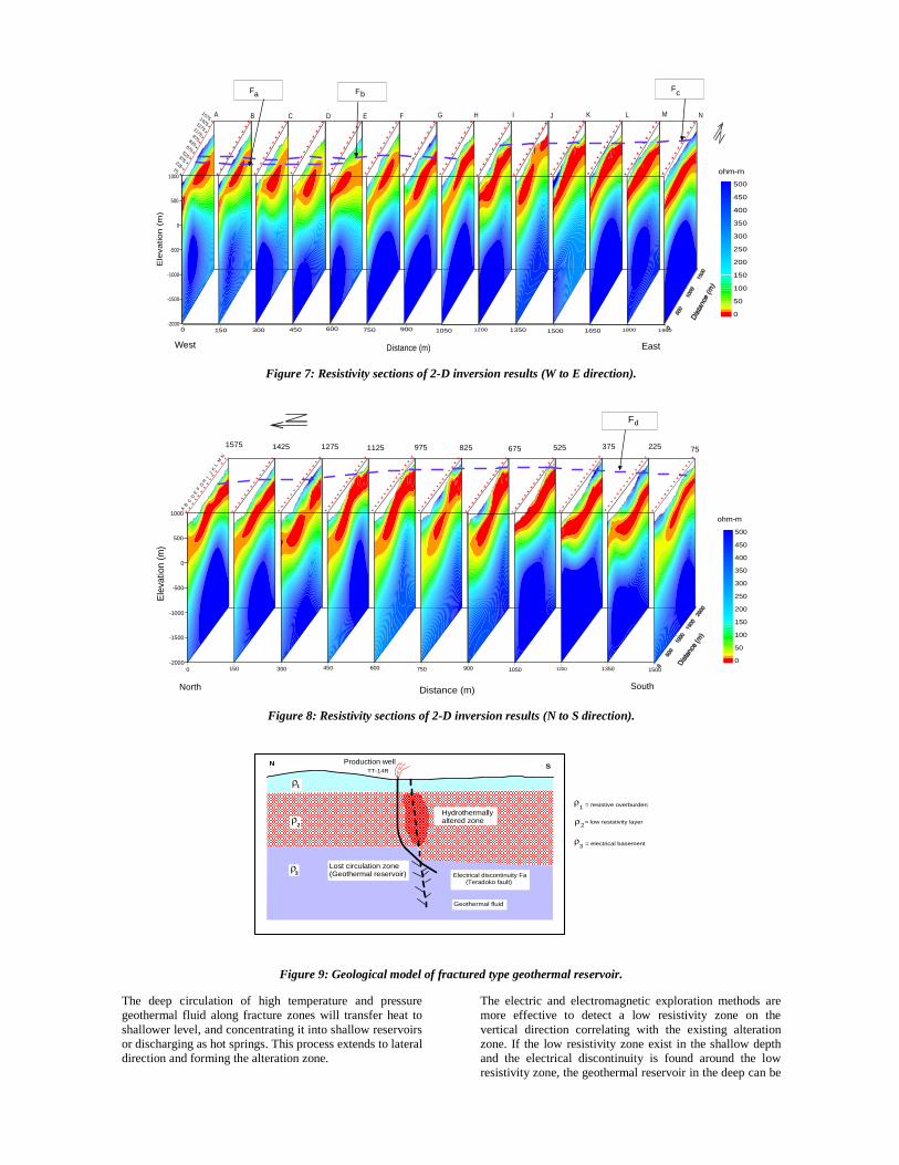
Fig.5 shows the 2-D resistivity sections in south to north direction of Line-A (Fig.5(a)) and B (Fig.5(b)) with survey lines as shown in Fig.2. There are two types of the electrical discontinuities found in those lines, that is Fa and Fb. The electrical discontinuity Fa clearly can be seen in the southwestern part of the survey area that is coincident with Teradoko fault. On the other hand, Fb is a remarkable electrical discontinuity in the area where the low resistivity is distributed broadly in the area in which the possible and close relation of a high geothermal activity may exist. The electrical discontinuities Fa and Fb extend from west to east up to Line-E and Line-H, respectively (Fig.7). In west to east direction, it is recognized also the electrical discontinuity Fc, which is located in the center of survey area from sites I-825 to N-825 (Fig.7). This area also has a high possibility of presence of geothermal reservoir.
2-D resistivity sections of Line-675 and Line-825 in west to east direction are also displayed in Fig.6. The figure
shows that there is electrical discontinuity Fd which is shown clearly below site K-675 (Fig.6(a)) and K-875 (Fig.6(b)). The Fd is also a remarkable electrical discontinuity because it is coincident with the position of Noine fault zone, extending from south to north (Fig.8). This fault divides the area into two parts, western and eastern part. It is clearly shown in the Figs.6(a) and (b) that the distribution of low resistivity is shallow and thin in the east and deepen and become thicker in the west. Accordingly, the underlain resistive layer correlated to the reservoir zone is shallower in the eastern part that that in the western part. This condition is similar with the interpretation of MT results for the survey line of SW-NE direction that the low resistivity in the second layer is shallow and thin in the northeast and become deeper and thicker in the southwest. The boundary of this condition is a Noine fault zone (Mustopa, et.al., 2001). From these results, it may conclude that the geoelectrical structure of fractured type geothermal reservoir can be explained by the model as shown in the Fig.9.
(a)Line-A (b)Line-B
Figure 5: Resistivity profiles (S-N) direction based on 2-D inversion of CSAMT data with electrical discontinuities Fa and Fb.
(a)Line-675 (b)Line-825
Figure 6: Resistivity profiles (W-E) direction based on 2-D inversion of CSAMT data with electrical discontinuities Fd.
Ele
va
tio
n (
m)
Distance (m)
0
50
100
150
200
250
300
350
400
450
500
ohm-m
A B C D E F G H I J K L M N
1000
500
0
-500
-1000
-1500
-20000 150 195018001650135012001050300 450 600 750 900 1500
75
225
375
525
675
825
975
1175
1275
1425
1575
West East
Fa FbFc
Figure 7: Resistivity sections of 2-D inversion results (W to E direction).
Ele
vatio
n (m
)
Distance (m)
0
50
100
150
200
250
300
350
400
450
500
ohm-m
752253755256758259751125127514251575
1000
500
0
-500
-1000
-1500
-20000 150 135012001050300 450 600 750 900 1500
AB
CD
EF
GH
IJ
KL
MN
Fd
North South
Figure 8: Resistivity sections of 2-D inversion results (N to S direction).
ρ1 = resistive overburden
ρ2= low resistivity layer
ρ3 = electrical basement
Production wellTT-14R
N S
Hydrothermallyaltered zone
Electrical discontinuity Fa (Teradoko fault)
Lost circulation zone(Geothermal reservoir)
ρ1
ρ2
ρ3
Geothermal fluid
Figure 9: Geological model of fractured type geothermal reservoir.
The deep circulation of high temperature and pressure geothermal fluid along fracture zones will transfer heat to shallower level, and concentrating it into shallow reservoirs or discharging as hot springs. This process extends to lateral direction and forming the alteration zone.
The electric and electromagnetic exploration methods are more effective to detect a low resistivity zone on the vertical direction correlating with the existing alteration zone. If the low resistivity zone exist in the shallow depth and the electrical discontinuity is found around the low resistivity zone, the geothermal reservoir in the deep can be
predicted. Therefore, the geothermal reservoir in Takigami geothermal field may exist around the electrical discontinuities Fa, Fb, Fc and Fd. This condition is similar to a geothermal system in Hatchobaru area obtained from interpretation of resistivity data (Ushijima et al., 1984).
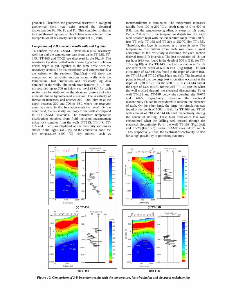
Comparison of 2-D inversion results with well log data
To confirm the 2-D CSAMT inversion results, resistivity well log and the temperature data from wells TT-13S, TT-14R, TT-16S and TT-20 are displayed in the Fig.10. The resistivity log data plotted with a semi log scale in ohm-m versus depth is put together in the same scale with the resistivity section. The lost circulation and temperature data are written on the sections. Figs.10(a) – (d) show the comparison of resistivity sections along wells with the temperature, lost circulation and resistivity log data obtained in the wells. The conductive features (3 –15 om-m) recorded up to 700 m below sea level (BSL) for each section can be attributed to the abundant presence of clay minerals due to hydrothermal alteration. The resistivity of formation increases, and reaches 200 – 300 ohm-m at the depth between 300 and 700 m BSL where the reservoir zone may exist in this formation (resistive layer). On the other hand, the resistivity well logs of the wells correspond to 2-D CSAMT inversion. The subsurface temperature distributions obtained from fluid inclusion measurement using rock samples from the wells (TT13S, TT-14R, TT-16S and TT-20) are displayed on the resistivity sections as shown in the Figs.10(a) – (d). At the conductive zone, the low temperature (100 oC) clay mineral such as
montmorillonite is dominated. The temperature increases rapidly from 100 to 200 oC at depth range of 0 to 400 m BSL that the temperature gradient is steep in this zone. Below 700 m BSL, the temperature distribution for each well becomes high with the temperature range from 230 oC (for TT-14R, TT-16S and TT-20) to 250 oC (for TT-13S). Therefore, this layer is expected as a reservoir zone. The temperature distributions from each well have a good correlation to the resistivity distribution for each section derived from 2-D inversion. The lost circulation of 18 ton per hour (t/h) was found in the depth of 500 m BSL for TT-13S (Fig.10(a)). For TT-14S, the lost circulation of 12 t/h occurred at the depth of 600 m BSL (Fig.10(b)). The lost circulation of 13.8 t/h was found at the depth of 200 m BSL for TT-16S and TT-20 (Figs.10(a) and (b)). The interesting point is found that the large lost circulation occurred at the depth of 1200 m BSL for the well TT-13S (114 t/h) and at the depth of 1300 m BSL for the well TT-14R (90 t/h) when the well crossed through the electrical discontinuity Fb in well TT-13S and TT-14R below the sounding site G-675 and G-825, respectively. Therefore, the electrical discontinuity Fb can be considered to indicate the presence of fault. On the other hand, the large lost circulation was found at the depth of 1000 m BSL for TT-16S and TT-20 with amount of 210 and 144 t/h mud, respectively, during the course of drilling. These high mud-water loss was encountered when the drilling well crossed through the electrical discontinuity Fc in the well TT-16S (Fig.10(c)) and TT-20 (Fig.10(d)) under CSAMT sites J-1125 and J-1425, respectively. Thus, the electrical discontinuity Fc also has a high possibility of promising fractures.
0
50
100
150
200
250
300
350
400
450
500
ohm-m
1000
500
0
-500
-1000
-1500
-2000
1 10 100 1000
Reistivity (ohm-m)NED-225 E-225 F-525 G-525 G-675 H-825 I-975
0 500 1000-2000
-1500
-1000
-500
0
500
1000
Fb
TT-13S
SW
Distance (m)
Ele
vatio
n (m
)
150 oC
100 oC
200 oC
114 t/h
18 t/h
250 oC
0
50
100
150
200
250
300
350
400
450
500
ohm-m
1000
500
0
-500
-1000
-1500
-2000
1 10 100 1000
Resistivity (ohm-m)
0 500 1000-2000
-1500
-1000
-500
0
500
1000C-525 D-525 E-675 F-675
H-825I-975
B-375 G-825
Fb
TT-14R
SW NE
Distance (m)
Ele
vatio
n (m
)
90 t/h
150 oC
230 oC
200 oC
100 oC
12 t/h
(a) TT-13S (b)TT-14R
0
50
100
150
200
250
300
350
400
450
500
ohm-m
1000
500
0
-500
-1000
-1500
-2000
1 10 100 1000
Reistivity (ohm-m)
0 500-2000
-1500
-1000
-500
0
500
1000G-1425 H-1425 I-1275 J-1125 K-975 L-975F-1575
Fc TT-16s
NW SE
Distance (m)
Ele
vatio
n (m
)
9.6 t/h100 oC
150 oC
230 oC
200 oC
13.8 t/h
210 t/h
0
50
100
150
200
250
300
350
400
450
500
ohm-m
1000
500
0
-500
-1000
-1500
-2000
1 10 100 1000Resistivity (ohm-m)
Distance (m)
Ele
vatio
n (m
)
0 500 1000-2000
-1500
-1000
-500
0
500
1000G-1575 H-1425 I-1425 J-1425 K-1275 L-1275F-1575 L-1125
Fc
TT-20
NW SE
9.6 t/h
100 oC
150 oC
230 oC
200 oC 27.6 t/h
34.8 t/h
144 t/h
(c)TT-16S (d)TT-20
Figure 10: Comparison of 2-D inversion results with the temperature, lost circulation and electrical resistivity log.
CONCLUSIONS
Employing a 2-D inversion to CSAMT data, we have successfully obtained the reasonable resistivity structure. The results are compared to real geological condition confirmed by drilling and indicated four remarkable electrical discontinuities that may correlate with fractures in the area. Highly correlation has been found between 2-D inversion results and well log data (electrical resistivity log, temperature and lost circulation data). Especially, the electrical discontinuities obtained from 2-D resistivity section are coincided with the zones of good lost circulation, which can be considered to highly indication of potential fractures.
Generally, the subsurface resistivity structures in Takigami geothermal filed are composed mainly by three types of resistivity feature, which are supported by both the 2-D inversion results of CSAMT data and resistivity logs (Figs.10(a) – (d)). The features of resistivity structure correlating with type of rocks and temperature distributions can be explained as follows; (1) The overburden (first layer) has a resistivity of 30 – 500 ohm-m and thickness of 300 to 500 m. This layer correlates with Noine-dake volcanic rock as non-altered zone and low temperature zone (50 oC) due to cold meteoric water circulation. (2) The intermediate (second) layer has an extremely low resistivity of 3 – 15 ohm-m that is 800 – 1000 m thick. The low resistivity layer as an anomalous feature can be considered as a hydrothermally altered zone (impermeable layer/cap rock). The second layer corresponds to Kusu, Ajibaru and Takigami formation composed of smectite and mixed clay minerals. The temperature distribution in the layer is characterized by a steep thermal gradient of about 20 oC/100 m. (3) The basement (third) layer is relatively more resistive than the second layer with resistivity of 30 - 500 ohm-m. This layer correlates with Mizuwake andesite rock, an illite-chlorite layer and high temperature zone (160 - 250
oC).
ACKNOWLEDGMENTS
We would like to express our gratitude to Idemitsu Oita Geothermal Co., Ltd. for provision of the CSAMT data and permission to release it in this paper.
REFERENCES
Bartel, L. C., and Jacobson, R. D., 1987, Results of a controlled-source audio frequency magnetotelluric survey at the Puhimau thermal area, Kilauea Volcano, Hawaii: Geophysics, 52, 665-677.
deGroot-Hedlin, C., and Constable, S., 1990, Occam’s inversion to generate smooth, two-dimensional models from magnetotelluric data: Geophysics, 55, 1613–1624.
Furuya, S., 1988, Geothermal resources of Takigami field, Japan, Proceeding of Int. Geothermal Symp., Kumamoto and Beppu, Japan, 119 - 120.
Furuya, S., Aoki, M., Gotoh, H., and Takenaka, T., 2000, Takigami geothermal system, northeastern Kyushu, Japan: Geothermics, 29, 191-211.
Goldstein, M. A., and Strangway, D. W., 1975, Audio-frequency magnetotelluric with a grounded electric dipole source: Geophysics, 40, 669-683.
Jupp, D. L. B. and Vozoff, K., 1986, Two-dimensional magnetotelluric inversion, in Vozoff, K, ed.
Magnetotelluric Methods: Geophysics Reprint, Series no. 5, Soc. Expl. Geophys, 460-479.
Kaufman, A. A., and Keller, G. V., 1983, Frequency and transient sounding method: Elsevier Science Publ. Co. Inc.
Mustopa, E. J., Furuya, S., Jotaki, H., and Ushijima, K., 2001, Subsurface imaging of Takigami geothermal field derived from magnetotelluric data: Geothermal and Volcanological Research Report of Kyushu University, 10, 77-96.
Rodi, W., and Mackie, R.L., 2001, Nonlinear conjugate gradients algorithm for 2-D magnetotelluric inversion, Geophysics, 66, 174-187.
Sandberg, S. K., and Hohmann, G. W., 1982, Controlled-source audio-magnetotelluric in geothermal exploration: Geophysics, 47, 100-116.
Sasaki, Y., 1989, Two-dimensional joint inversion of magnetotelluric and dipole-dipole resistivity: Geophysics, 55, 682-694.
Sasaki, Y., Yoshihiro, Y., and Matsuo, K., 1992, Resistivity imaging of controlled-source audiofrequency magnetotelluric data: Geophysics, 57, 952-955.
Smith, J. T. and Booker, J. R., 1991, Rapid inversion of two- and three-dimensional magnetotelluric data: J. Geophys. Res., 96, 3905-3922.
Takenaka, T., and Furuya, S., 1991, Geochemical model of the Takigami geothermal system, northeast Kyushu, Japan: Geochemical Journal, 25, 267-281.
Uchida, T, 1993, Smooth 2-D inversion for magnetotelluric data based on statistical criterion ABIC: J. Geomag. Geoelectr., 45, 841-858.
Unsworth, M. J., Lu, X., and Watts, M. D., 2000, CSAMT exploration at Sellafield: Characterization of a potential radioactive waste disposal site: Geophysics, 65, 1070-1079.
Ushijima, K., Yuhara, K., Tagomori, K., and Inoue, K., 1984, Anisotropic resistivity inversion of VES curve at Hatchobaru geothermal field, Japan: Geothermal Resources Council Transactions, Vol. 8, 517-522.
Yamashita, M., Hallof, P. G., and Pelton, W. H., 1985, CSAMT case histories with a multichannel CSAMT system and near-field data correction: 55th SEG Annual Convention, 276-278.
Zonge, K. L., and Hughes, L. J., 1991, Controlled source audio-frequency magnetotellurics, in Nabighian, M. N., Ed., Electromag-netic methods in applied geophysics, 2: Soc. Expl. Geophys.
Zonge, K. L., Ostrander, A. G., and Emer, D. F., 1986, Controlled-source audiofrequency magnetotelluric measurements, in Vozoff, K., Ed., Magnetotelluric methods: Soc. Expl. Geophys. Geophysics Reprint Series 5, 749-763.