Image theory for reflected TE/TM wave in waveguide

IEEE TRANSACTIONS ON MICROWAVE THEORY AND TECHNIQUES, VOL. 46, NO. 1, JANUARY 1998 55

Image Theory for Reflected TE/TMWave in Waveguide

Perttu P. Puska and Ismo V. Lindell,Fellow, IEEE

Abstract— The image principle is extended to thetime–harmonic problem of TE/TM wave propagation andreflection in a waveguide. The fictitious image generating thereflected field is derived with the aid of Heaviside operationalcalculus and a transmission-line model of the waveguide. Theoperational calculus reveals that the image of a point-like sourcein front of the waveguide discontinuity is another point-likesource in the mirror-image position and a line source extendingfrom the mirror-image position to infinity. The image derivedwith operational calculus turns out to be independent of thewaveguide’s transverse geometry.

Index Terms—Electromagnetic analysis, electromagnetic reflec-tion, electromagnetic scattering, transmission-line discontinuities,transmission-line theory.

I. INTRODUCTION

PROBLEMS concerning TE or TM wave reflection in awaveguide are usually tackled with methods that are of

approximate nature—the waveguide is somehow discretizedand the fields are solved numerically, Huygens sources areused on the interface, etc. On the other hand, the image theorygives exact solutions, provided that the images can be found.The lack of a suitable method for finding the images is thereason that the image theory has not been widely used inwaveguide problems. However, this paper proposes an easyway to derive the images, with the use of an old, but inits directness, attractive method—the Heaviside operationalcalculus [1], [2]. With only a few manipulation steps, thecalculus gives an operational form of the image expressionthat can be evaluated in some cases even in a closed form.The one case where the closed-form expression is possibleis the problem of the TE/TM wave reflection in a waveguidewith an abrupt change in the waveguide longitudinal parameterprofile. Before applying Heaviside operational calculus to thisproblem we must, in one way or another, cast the waveguidegeometry in one-dimensional (1-D) or-dependent form, sothat the reflection operators acting on-dependent generalizedfunctions can be applied. With transmission-line formalismgiven in the Appendix, we can reduce a waveguide probleminto a 1-D problem—and that is how we start in Section II. Wethen derive the images in Section III and finally, in Section IV,consider an example in rectangular geometry.

II. SERIES EXPANSIONS FOR THEFIELD AND THE SOURCE

Let us first find the modal representation of the scalar fieldin the waveguide with cross sectionand boundary . The

Manuscript received December 5, 1996; revised October 9, 1997.The authors are with the Electromagnetics Laboratory, Helsinki University

of Technology, FIN-02150 Espoo, Finland.Publisher Item Identifier S 0018-9480(98)00629-2.

field is a solution of the inhomogenous Helmholtz equation

(1)

and, furthermore, satisfies either Neumann- or Dirichlet-typeboundary conditions on . We assume that and sourcecan be written as

(2)

where ’s are orthonormal in the sense

(3)

and satisfy the transverse eigenvalue equation

(4)

Substituting (2) into (1) gives

(5)

where denotes the double sum of (2). Operating (5) fromleft with and using (3) and (4) finally yields

(6)

where . The assumption of the separability ofand enables us to reduce the problem to a transmission-line

one, where plays a role of mode voltage or current waveand generally represents a combined voltage and currentsource for mode . With the waveguide reflection problemin the mind, we let (6) describe the mode voltage/current

due to source located in the region ,and we then let be incident on interface atafter which the waveguide parameters abruptly change. Thechange in the parameters naturally gives rise to reflected modevoltage/current wave (as well as alters the incident wavetraveling to the negative -direction). The reflected modalwave can be thought of as being produced by sourcein theregion if the interface is removed and the transmissionline is extended to the region . Now the reflected-mode voltage/current is given by

(7)

with the usual solution that we may try to write in thefollowing form:

(8)

0018–9480/98$10.00 1998 IEEE

56 IEEE TRANSACTIONS ON MICROWAVE THEORY AND TECHNIQUES, VOL. 46, NO. 1, JANUARY 1998

where, in fact, and, thus,the substitution of (8) into (7) gives

(9)

However, the right-hand side (RHS) of (9) is nothing else but

(10)

because of (6)

III. I MAGE SOURCE THROUGH

HEAVISIDE OPERATIONAL CALCULUS

A. Identification of Propagation Coefficientswith Differential Operators

The RHS of (10) givesan operational formof the reflectionimage source as follows:

(11)

The termoperationalcould be understood by considering theexp-dependence of the solutions of (6) or (7), which allowsus to identify

(12)

and by supposing that the reflection coefficient of the modecan be expanded as a power series of . The operational

form of the reflection coefficient is then a pseudo-differentialoperator , where every has been replaced by .As was not a function of the indices , but ratherof , the resulting does not depend on the indices

or, in other words, are similar in form for allmodes and, consequently, all the modes have the sameoperational expression for the reflection coefficient.

Thus, if the series expansion of is, the image has the expression

(13)

The image source for the total reflected field isthen

(14)

where stands for the reflection dyadic . Equation(14) actually claims that the image is independent of thewaveguide transverse geometry since the guide geometryparameters do not appear in the operational expression. Thisrather surprising result is mathematically due to the fact thatwe could pull the reflection operator out of the sum in (14), butthe physical reason for this can be seen if we apply the image

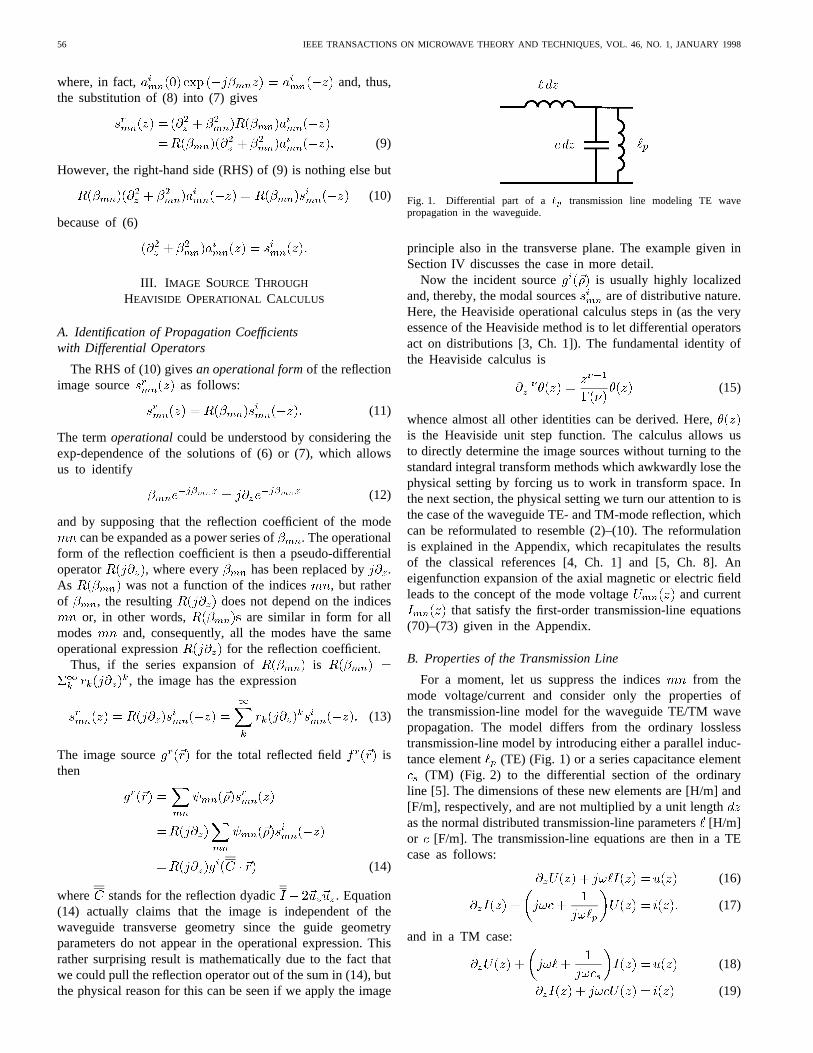
Fig. 1. Differential part of a`p transmission line modeling TE wavepropagation in the waveguide.

principle also in the transverse plane. The example given inSection IV discusses the case in more detail.

Now the incident source is usually highly localizedand, thereby, the modal sources are of distributive nature.Here, the Heaviside operational calculus steps in (as the veryessence of the Heaviside method is to let differential operatorsact on distributions [3, Ch. 1]). The fundamental identity ofthe Heaviside calculus is

(15)

whence almost all other identities can be derived. Here,is the Heaviside unit step function. The calculus allows usto directly determine the image sources without turning to thestandard integral transform methods which awkwardly lose thephysical setting by forcing us to work in transform space. Inthe next section, the physical setting we turn our attention to isthe case of the waveguide TE- and TM-mode reflection, whichcan be reformulated to resemble (2)–(10). The reformulationis explained in the Appendix, which recapitulates the resultsof the classical references [4, Ch. 1] and [5, Ch. 8]. Aneigenfunction expansion of the axial magnetic or electric fieldleads to the concept of the mode voltage and current

that satisfy the first-order transmission-line equations(70)–(73) given in the Appendix.

B. Properties of the Transmission Line

For a moment, let us suppress the indices from themode voltage/current and consider only the properties ofthe transmission-line model for the waveguide TE/TM wavepropagation. The model differs from the ordinary losslesstransmission-line model by introducing either a parallel induc-tance element (TE) (Fig. 1) or a series capacitance element

(TM) (Fig. 2) to the differential section of the ordinaryline [5]. The dimensions of these new elements are [H/m] and[F/m], respectively, and are not multiplied by a unit lengthas the normal distributed transmission-line parameters[H/m]or [F/m]. The transmission-line equations are then in a TEcase as follows:

(16)

(17)

and in a TM case:

(18)

(19)

PUSKA et al.: IMAGE THEORY FOR REFLECTED TE/TM WAVE IN WAVEGUIDE 57

Fig. 2. Differential part of acs transmission line modeling TM wavepropagation in the waveguide.

assuming a time variance. The source terms ,represent a distributed series voltage source and a distributedparallel current source. The propagation coefficientsare now

TE

TM (20)

and corresponding characteristic admittances/impedances

TE

TM (21)

It is seen that there is a relation betweenand :

TE TM (22)

The inhomogenous Helmholtz equations for the andare found from (16) to (19) as follows:

(23)

(24)

C. and Generated by Sources

The solution of (23) or (24) can be written as a convolutionof the source with Green function, and after partial integrationthe convolution integrals become

(25)

(26)

We rewrite (25) and (26) to reveal that or actuallydescribe two wavefronts traveling to opposite directions:

(27)

(28)

Fig. 3. Image principle inp line. The upper section depicts the situation ofthe original problem with two differentp transmission lines joined atz = 0

and the source atz = z0: In the lower section, the boundary is removedand the left-hand transmission line of the upper section is replaced by a linehaving the same parameters as the right-hand transmission line. However, thefields in the regionz > 0 do not change because we have placed images in theleft half-space. The image source starts fromz = �z0 and extends to�1.

D. Two Transmission Lines

Having established the parameters of the transmission linecorresponding to the TE/TM mode propagation, we may thenapply operational calculus to the problem described in theSection II—the case of mode voltage or current wave reflec-tion and transmission from the junction of two transmissionlines. The full problem splits into two parts: the TE partcorresponding to the case where two lines with differentcharacteristics are connected at and the TM part, wheretwo lines are similarly joined together. In both cases, theline with impedance is located in the region andthe line with in . The source is a sum of current

and voltagegenerators with infinite and zero internal impedances, respec-tively. The upper part of the Fig. 3 describes the situation.A current–voltage source just described is chosen because itis of the most elementary form, producing only left-goingwaves traveling toward the interface, provided that we set

. Equations (27) and (28) then give

(29)

1) TE Modes: The reflection and transmission coefficientsin the line corresponding to the TE case read

(30)

(31)

where we have used (22). In an ordinary transmission-lineproblem, and would have been independent of propaga-tion coefficients and, consequently, the analysis would lead toalmost trivial image sources, e.g., the reflected voltage imagewould simply be a mirror image of the original one. However,the situation depicted in (30) and (31) leads to distributedimage sources as will be seen shortly. Equations (30) and (31)can be written in a form involving only either one of thepropagation coefficient by requiring the transverse componentof the wavenumber vector to be continuous:

(32)


where . Hence, (30) can be written inthe form

(33)

Before proceeding, we note that (23) and (24) for the voltageand current are similar in form and, consequently, we onlyneed to analyze the case of the reflected voltage wave—thecurrent wave may be inferred by suitable changes of thevariables. In order for the reflected wave to appear, the incidentwave is needed:

(34)

and we wish to find the image sourceof the reflected wavesgiven by

(35)

The reflected voltage can be given in the operational form

(36)

(37)

Substituting (37) in (35) yields

(38)

where the last expression is the operational form of the image,which can be written as

In operating on the source termwith we need the formula

(39)

where [2], [6, pp. 238–239]

(40)

and denotes the Heaviside unit step function (see Fig. 4).A word of caution concerning the substitution of the inradicals as is in place here: we must choosethe sign of the radical so that the result makes sense physically.Unfortunately, we have no way of knowing the sign otherthan by examining which one makes more sense physically.We can, for instance, examine what happens when .In this case, the inspection reveals that

. The ambiguity arises from the fact that thereis no unique image for the reflected field even though the

Fig. 4. Function�(�; z) forming the continuous part of the RHS of (39)with different values of�.

reflected field itself must have a unique solution in the region.

Thus, the expression for the voltage image is

(41)

where

(42)

(43)

From (41) to (43), it is seen that the reflection images aregenerally combined of poles and continuous line sources,where the line sources start from and extend to

(see Fig. 3).The complete treatment of the problem requires a transmis-

sion image too, with the image now being found through theuse of the operator (31). Applying the property (32) yields forthe transmission operator

We assumed that the reflected voltage can be given by (35).Likewise, we assume that the transmitted voltage is a solutionof

(44)

To simplify the manipulations appearing in the steps to followwe introduce a “modified” incident wave:

where , and which has a solution

(45)

Requiring to be continuous across the interface gives


which combined with (44) and (45) gives

(46)

where we have used the Heaviside shifting property. We note that (44) and (46) should

describe the same source. The relation (46) needs only asuitable replacement for ’s. The apparent choice for thereplacement is because the transmitted wave is goingleft. Therefore,

and

2) TM Modes: We may instantly write down solutions cor-responding to the line image problem by using the solutionsof the TE problem if the following dualities between TE andTM transmission lines are recognized:

E. Waveguide Images

The images we have considered earlier were derived withrespect to general properties of the transmission line. If theyrepresent modal images , the entire image for the reflected

field is then a sum of these modal TE images:

(47)

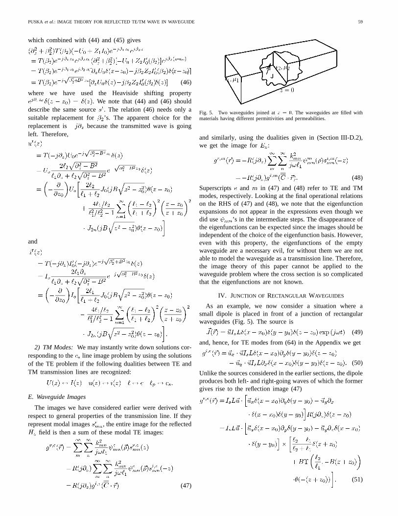
Fig. 5. Two waveguides joined atz = 0. The waveguides are filled withmaterials having different permittivities and permeabilities.

and similarly, using the dualities given in (Section III-D.2),we get the image for :

(48)

Superscripts and in (47) and (48) refer to TE and TMmodes, respectively. Looking at the final operational relationson the RHS of (47) and (48), we note that the eigenfunctionexpansions do not appear in the expressions even though wedid use ’s in the intermediate steps. The disappearance ofthe eigenfunctions can be expected since the images should beindependent of the choice of the eigenfunction basis. However,even with this property, the eigenfunctions of the emptywaveguide are a necessary evil, for without them we are notable to model the waveguide as a transmission line. Therefore,the image theory of this paper cannot be applied to thewaveguide problem where the cross section is so complicatedthat the eigenfunctions are not known.

IV. JUNCTION OF RECTANGULAR WAVEGUIDES

As an example, we now consider a situation where asmall dipole is placed in front of a junction of rectangularwaveguides (Fig. 5). The source is

(49)

and, hence, for TE modes from (64) in the Appendix we get

(50)

Unlike the sources considered in the earlier sections, the dipoleproduces both left- and right-going waves of which the formergives rise to the reflection image (47)

(51)


Fig. 6. The original and the image source (line image part only shown).

The source (see Fig. 6) of the-component of the reflected-field is then a combination of: 1) a point source located

at , , and is otherwise similar to theoriginal source, but the amplitude is modified by the factor

and 2) a line source starting from ,, and extending to the infinity in the negative

-direction. The line source has an amplitude variation givenby

In the case of the rectangular guide, there is a nice explana-tion for the independence of (51) of the transverse coordinates

, —we can picture that in addition to the original imagethere is an infinite set of images placed in the mirror-imagepoints in the transverse plane of the guide (Fig. 7). Images inthe transverse plane extend longitudinally to the infinity in asimilar fashion as the original one (51).

V. CONCLUSION

Solving waveguide discontinuity problems such as the onedemonstrated here usually involve the construction of theGreen function for the waveguide. The geometry of thediscontinuity has to be built into the Green function in orderfor the Green function to satisfy boundary conditions. Workrequired to develop the Green function for the simple examplepresented in this paper might be within reasonable limits, butcertainly not for more complicated settings such as scatterersin the waveguide near the discontinuity. The image-theoryapproach needs only an empty waveguide’s Green function,and the previous problem of forming the Green functionsatisfying boundary conditions reduces to the case of findingthe images. Once the images sources are found with theprocedure described in the previous sections, the fields areimmediately obtained by simply taking the convolution of allsources with the Green function of the empty waveguide.The practicability of this approach is seen clearly if, forinstance, we are writing a program to calculate fields inwaveguide scattering problems. We need write only one simplesubroutine for the Green function no matter the number andshape of the scatterers. Now the principal work is to formthe image sources, and here the Heaviside calculus may beapplied. The way Heaviside calculus was used in the previoussections can be classified as a direct-type formulation of thegeneral image theory. The other class of general image-theoryformulations can be termed as being of the integral transformtype. An example of the latter category is the exact imagetheory (EIT) that used Laplace transform techniques to findthe images [7]. The disadvantage of the EIT was that the

(a) (b)

Fig. 7. (a) Rectangular waveguide’s walls can be removed if infinite numberof image sources similar to the original one are substituted in the (b) transversemirror-image positions.

manipulations of integrals of Laplace transforms could be quitetedious. But, as we have seen in this paper, Heaviside calculusgives operational expressions for the images immediately anddeals naturally with the distributive nature of the sources. Aparticularly attractive feature is that Heaviside calculus leadsto physically sound images in the sense that the images arecombinations of point-like sources that could be called “static,”existing even when , and line sources that could bethought of as being “dynamic” additions to the “static” images.After all, intuition shows that time–harmonic images shoulddiffer from the time-independent ones, yet the images shouldbear some resemblance to the images of the static problem.

APPENDIX

TRANSMISSION-LINE MODEL FOR TE/TM MODES

A. Mode Voltages and Currents

In a waveguide TE- or TM-mode propagation case, theelectric and magnetic fields can be conveniently expressedwith scalar transverse eigenfunctionand scalar longitudinaleigenfunction [5, Ch. 8], and for a single mode’s electricand magnetic field we have the following relations, where thedouble mode indices are suppressed:

(52)

(53)

(54)

(55)

The TM case is dual to the previous one, hence,

(56)

(57)

(58)

Now connecting with or , (52)–(58) appear as

(59)

(60)


where mode voltages or currents and mode vectors are

(61)

The mode vectors thus expressed are orthogonal and areassumed to be normalized over the cross-sectional area ofguide.

B. Sources

The relation between transmission-line sources ,and current or magnetic current remains to befound. To this end we start with Helmholtz equations for,

:

(62)

(63)

and proceed by taking the-components of the aforementionedquantities, since it is possible to express TE or TM fields asfunctions of longitudinal fields only:

(64)

(65)

Substituting the series expansions

(66)

(67)

(where is the cutoff wavenumber of the mode) in(64)–(65), multiplying from the left by , and integratingover the cross section eventually yields

(68)

C. Circuit Components

It is seen from (61) that one may define mode impedances

(69)

Equation (61), combined with (68), finally yield thetransmission-line equations with sources

(70)

(71)

for TE and

(72)

(73)

for TM. Comparing (70) and (71) with (16) and (17), and(72) and (73) with (18) and (19), one recognizes the followingcorrespondences:

(74)

REFERENCES

[1] O. Heaviside,Electromagnetic Theory, 2nd. ed., vols. 1–3. London,U.K.: Ernest Benn, 1925.

[2] I. V. Lindell, “Heaviside operational calculus in electromagnetic imagetheory,” J. Electromagn. Waves Applicat., vol. 11, no. 1, pp. 119–132,1997.

[3] E. J. Berg, Heaviside’s Operational Calculus, 2nd ed. New York:McGraw-Hill, 1936.

[4] N. Marcuvitz, Waveguide Handbook. New York: McGraw-Hill, 1951.[5] R. F. Harrington,Time–Harmonic Electromagnetic Fields. New York:

McGraw-Hill, 1961.[6] I. V. Lindell, Methods for Electromagnetic Field Analysis, 2nd ed.

Piscataway, NJ: IEEE Press, 1995.[7] I. V. Lindell and E. Alanen, “Exact image theory for the Sommerfeld

half-space problem—Part I: Vertical magnetic dipole,”IEEE Trans.Antennas Propagat., vol. AP-32, pp. 126–133, Feb. 1984.

Perttu P. Puska received the M.Sc. degree in electrical engineering fromHelsinki University of Technology (HUT), Espoo, Finland, in 1995, and iscurrently working toward the Ph.D. degree at the Electromagnetics Laboratory,HUT.

Ismo V. Lindell (S’68–M’69–SM’83–F’90) was born in Viipuri, Finland, in1939. He received the Dr.Tech. (Ph.D.) degree from Helsinki University ofTechnology (HUT), Espoo, Finland, in 1971.

He is currently a Professor of electromagnetic theory at the Electromag-netics Laboratory, HUT, and holds the research position of Professor of theAcademy of Finland. He has authored or co-authored scientific papers andbooks, includingMethods for Electromagnetic Field Analysis,(Piscataway, NJ,IEEE Press, 1995),Electromagnetic Waves in Chiral and Bi-Isotropic Media(Norwood, MA: Artech House, 1994), andHistory of Electrical Engineering(in Finnish) (Finland: Otatieto, 1994).

Dr. Lindell is chairman of Commission B of the URSI National Committeeof Finland.

Documents

Image theory for reflected TE/TM wave in waveguide