Embed Size (px)
Citation preview
Technical Report 19, The Ohio State University Center for Cognitive Science, 1996
Cognitive Science Technical Report #19, April 1996Center for Cognitive Science
The Ohio State University208 Ohio Stadium East1961 Tuttle Park Place
Columbus, OH 43210-1102, U.S.A.PH: 614-292-8200 FX: 614-292-0321
EML: [email protected]
Image Segmentation Based on Oscillatory Correlation
DeLiang Wang† and David Terman‡
†Department of Computer and Information Science and Center for Cognitive Science‡Department of Mathematics
The Ohio State University, Columbus, Ohio 43210, USA
AbstractWe study image segmentation on the basis of locally excitatory globally inhibitory oscillatornetworks (LEGION), whereby the phases of oscillators encode the binding of pixels. Weintroduce a potential for each oscillator so that only those oscillators with strong connections fromtheir neighborhood can develop high potentials. Based on the concept of potential, a solution toremove noisy regions in an image is proposed for LEGION, so that it suppresses the oscillatorscorresponding to noisy regions, without affecting those corresponding to major regions. We showanalytically that the resulting oscillator network separates an image into several major regions, plusa background consisting of all noisy regions, and illustrate network properties by computersimulation. The network exhibits a natural capacity in segmenting images. The oscillatorydynamics leads to a computer algorithm, which is applied successfully to segmenting real gray-level images. A number of issues regarding biological plausibility and perceptual organization arediscussed. We argue that LEGION provides a novel and effective framework for imagesegmentation and figure-ground segregation.

DeLiang Wang and David Terman Image Segmentation
2
1. IntroductionThe segmentation of a visual scene (image) into a set of coherent patterns (objects) is a
fundamental aspect of perception, which underlies a variety of tasks such as image processing,figure-ground segregation, and automatic target recognition. Scene segmentation plays a criticalrole in the understanding of natural scenes. Although humans perform it with apparent ease, thegeneral problem of image segmentation remains unsolved in sensory information processing. Asthe technology of single-object recognition becomes more and more advanced in recent years, thedemand for a solution to image segmentation is increasing since both natural scenes andmanufacturing applications of computer vision are rarely composed of a single object.
Objects appear in a natural scene as the grouping of similar sensory features and thesegregation of dissimilar ones. Sensory features are generally taken to be local, and in the simplestcase may correspond to single pixels. To approach the problem of scene segmentation, three basicissues must be addressed: What are the cues that determine grouping and segregation? What is theproper representation for the result of segmentation? How are the cues used to give rise tosegmentation?
Much is known about sensory cues that are important for segmentation. In particular, Gestaltpsychology has uncovered a set of principles guiding the grouping process in the visual domain(Wertheimer 1923; Koffka 1935; Rock and Palmer 1990). We briefly summarize some of themost important principles (see also Rock and Palmer 1990):
• Proximity. The closer the features lie to each other, the easier they are to be grouped into thesame segment.
• Similarity. Features that have similar attributes, such as grayness, color, depth, texture, etc.,tend to group together.
• Common fate. Features that have similar temporal behavior tend to group together. Forinstance, a group of features that move coherently (common motion) would form a single object.Notice that common fate may be regarded as one aspect of similarity. We list it separately toemphasize the importance of time as a separate dimension.
• Connnectedness. A uniform, connected region, such as a spot, line, or more extended area,tends to form a single segment.
• Good continuation. A set of features that form a smooth and continuous curve tend to grouptogether.
The above principles concern only the qualities within the input image. Such groupings maybe referred to as the bottom-up process. Another important aspect has to do with prior knowledge(memory), i.e., if a set of features belong to the same familiar pattern, they tend to group together.Prior knowledge can strongly influence the grouping process in a top-down fashion, and it is listedin the following.
• Prior knowledge.All of these principles (possibly more) work together to give rise to segmentation. The
integration of these differing principles by itself can pose a significant computational problem.In computer vision algorithms for image segmentation, the result of segmentation can be
represented in many ways. However, it is not a trivial task to represent the outcome ofsegmentation in a neural network. One proposal is naturally derived from the so-called neurondoctrine (Barlow 1972), where neurons at higher brain areas are assumed to become more selectiveand eventually a single neuron represents each single object. This representation is also called thegrandmother-cell representation. Multiple objects in a visual scene would be represented by thecoactivation of multiple units at some level of the nervous system. This representation faces majortheoretical and neurobiological problems (von der Malsburg 1981; Abeles 1991; Singer 1993).Another proposal relies on temporal correlation to encode the binding (Milner 1974; von derMalsburg 1981; Abeles 1982). In particular, the correlation theory of von der Malsburg (1981)

DeLiang Wang and David Terman Image Segmentation
3
asserts that an object is represented by the temporal correlation of the firing activities of thescattered cells that encode different features of the object. Multiple objects are represented bydifferent correlated firing patterns that alternate in time, each corresponding to a single object.
Temporal correlation provides an elegant way to represent the result of segmentation. A specialform of temporal correlation is oscillatory correlation, where the basic unit is a neural oscillator(see Terman and Wang 1995; Wang and Terman 1995). However, this representation does not,by itself, reveal how segmentation is achieved using Gestalt grouping principles. As a matter offact, despite an extensive body of literature dealing with segmentation using temporal correlation(starting perhaps from von der Malsburg and Schneider 1986), little progress has been made inbuilding successful neural systems for image segmentation. There are two major challenges facingthe oscillatory correlation theory. The first challenge is how to achieve fast synchronization withina population of locally coupled oscillators. Most of the models proposed for achieving phasesynchrony rely on all-to-all connections (see Sect. 2 for more details). However, as pointed outby Sporns et al. (Sporns et al. 1991) and Wang (Wang 1993a), a network with full connectionsindiscriminately connects all the oscillators which are activated simultaneously by different objects,because the network is dimensionless and loses critical information about geometry. The secondchallenge is how to achieve fast desynchronization among different groups of oscillatorsrepresenting distinct objects. This is necessary in order to segment multiple objects simultaneouslypresented.
We have previously proposed a neural network framework to deal with the problem of imagesegmentation, called Locally Excitatory Globally Inhibitory Oscillator Networks (LEGION) (Wangand Terman 1995; Terman and Wang 1995). Each oscillator is modeled as a standard relaxationoscillator. Local excitation is implemented by positive coupling between neighboring oscillatorsand global inhibition is realized by a global inhibitor. LEGION exhibits the mechanism of selectivegating, whereby oscillators stimulated by the same pattern tend to synchronize due to localexcitation and oscillator groups stimulated by different patterns tend to desynchronize due to globalinhibition (Wang and Terman 1995; Terman and Wang 1995). We have proven that, with theselective gating mechanism, LEGION rapidly achieves both synchronization within groups ofoscillators that are stimulated by connected regions and desynchronization between differentgroups. In sum, LEGION provides an elegant solution to both challenges outlined above.
In this paper, we study LEGION for segmenting real images. Before we demonstrate imagesegmentation, the original version of LEGION needs to be extended to handle images with manytiny (noisy) regions. One such example is shown in Fig. 1, where three objects with a noisybackground form a visual image. Without extension, LEGION would treat each region, no matterhow small it is, as a separate segment. Thus, it would lead to many tiny fragments. We call thisproblem fragmentation. Because different segments alternate in time, a large number of fragmentsslow down the segmentation process drastically. Another and more serious problem is that it isdifficult to choose parameters so that LEGION is able to achieve more than several (5 to 10)segments (Terman and Wang 1995). Noisy fragments may, therefore, compete with major imageregions for becoming segments, so that it may not be posssible to extract all of the major segmentsfrom an image. The problem of fragmentation is solved by introducing a concept of potential foreach oscillator. The stimulated oscillators that receive significant input from their neighborhoodswill develop high potentials, while other stimulated oscillators will not. Shortly after they arestimulated, low-potential oscillators that cannot be recruited by high-potential ones will ceaseoscillating. The extended dynamics is fully analyzed, and the resulting LEGION network isapplied to gray-level images and yields successful segmentation.
In the next section we review prior work relevant to image segmentation and neural networks,particularly neural models using the representation of oscillatory correlation. In Section 3, ourmodel is described in detail, and it is analyzed in Section 4. In Section 5, computer simulations ofthe extended LEGION network are presented. Section 6 presents the segmentation results on real
DeLiang Wang and David Terman Image Segmentation
4
images. Further discussions concerning our approach are given in Section 7. Finally, Section 8concludes our exposition.
2. Related Work2.1 Image Segmentation Algorithms
Due to its critical importance for computer vision, image segmentation has been studiedextensively. Many techniques have been invented (for reviews of the subject see Zucker 1976;Haralick 1979; Lowe 1985; Haralick and Shapiro 1985; Sarkar and Boyer 1993b; Pal and Pal1993). Broadly speaking, there are three categories of algorithms: pixel classification, edge-basedorganization, or region-based segmentation. A simple classification technique is thresholding: apixel is assigned a specific label if some measure of the pixel passes a certain threshold. This ideacan be extended to a complex form including multiple thresholds which are determined by pixelhistograms (Kohler 1981). This way, a region of pixels is grouped together if its pixels fallbetween two threshold values. Some learning techniques may be introduced to make classificationmore flexible (see Uchiyama and Arbib 1994, for example). Edge-based techniques generally startwith an edge-detection algorithm, which is followed by grouping edge elements into rectilinear orcurvilinear lines. These lines are then grouped into boundaries that can be used to segment imagesinto various regions (see, for example, Geman et al. 1990; Sarkar and Boyer 1993a; Foresti et al.1994). Finally, region-based techniques operate directly on regions. A classical method is regiongrowing/splitting (or split-and-merge, see Horowitz and Pavlidis 1976; Zucker 1976; Pavlidis1977; Adams and Bischof 1994), where iterative steps are taken to grow (split) pixels into aconnected region if all the pixels in the region satisfy some conditions. One such condition is thatthe distance between the minimum and the maximum pixel values is within a pre-defined range.Most of the techniques use one or more Gestalt grouping principles that emphasize relationshipsamong object components (Mohan and Nevatia 1989; Sarkar and Boyer 1993b).
One of the apparent deficits with these algorithms is their iterative (serial) nature (Liou et al.1991). There are some recent algorithms which are partially parallel. In Sha'ashua and Ullman(1988), a globally consistent curve structure is detected using a locally connected network. In Liouet al. (1991), a parallel technique is used to search a partition space. In Mohan and Nevatia(1992), part of the segmentation process is performed by a neural network for cost optimization.A similar approach is taken by Manjunath and Chellappa (1993), who use a competitive networkfor reducing noise and illumination effects. A parallelizable inference network based on Baysianstatistics is used by Sarkar and Boyer for detecting a set of structures, such as ellipses, circles, andribbons (Sarkar and Boyer 1993a).
Most of these techniques rely on domain-specific heuristics to perform segmentation, and nounified computational framework exists to explain the general phenomenon of scene segmentation(Haralick and Shapiro 1985). The problem of scene segmentation is computationally hard (Gurariand Wechsler 1982), and largely regarded unsolved.
2.2 Neural Network EffortsNeural networks have proven to be a successful approach to pattern recognition (Schalkoff
1992; Wang 1993b). Unfortunately, little work has been devoted to scene segmentation which isgenerally regarded as part of preprocessing (often meaning manual segmentation). Scenesegmentation is a particularly challenging task for neural networks, partly because traditional neuralnetworks lack the representational power for encoding multiple objects simultaneously. The twomost popular network architectures, namely multilayer perceptrons and associative memories, bothrequire learning or memory of patterns first, whereas scene segmentation, except that based onprior knowledge, seems to be an innate and immediate process, thus difficult to be formulated inthese architectures.

DeLiang Wang and David Terman Image Segmentation
5
Sejnowski and Hinton proposed a scheme for separating a figure from a background using theBolzmann machine algorithm (Sejnowski and Hinton 1987). Their method may reverse the figureand the background by shifting top-down input (they call it attention). Mozer et al. (1992)presented an interesting method of using multilayer perceptrons for scene segmentation, in whicheach unit is extended to code both intensity and phase. Grossberg and Wyse (1991) proposed amodel for image segmentation, based on the contour detection model of Grossberg and Mingolla(1985). The model uses filling-in (dye-spreading) to restore regions from closed contours.Computer simulations implementing some of the ideas proposed in Grossberg and Mingolla(Grossberg and Mingolla 1985) have been presented by Gove et al. (in press). However, all ofthese methods were tested only on small synthetic images, and it is not clear how they can beextended to handle real images.
Since neural networks can be readily applied to classification tasks, they are applicable tosegmentation based on pixel classification. In particular, Kohonen's self-organizing maps havebeen used for segmentation (Kohonen 1995). Koh et al. (1995) have developed a system based onself-organizing maps to segment range images. Raghu et al. (1995) have studied textureclassification using a self-organizing map followed by a multilayer perceptron. A primarydrawback of these methods is that the number of segments (objects) is assumed to be known apriori .
Because temporal (oscillatory) correlation offers an elegant way of representing multipleobjects in neural networks (von der Malsburg and Schneider 1986), most of the neural networkefforts on image segmentation have centered around this theme. In particular, the discovery ofsynchronous oscillations in the visual cortex has triggered much interest in exploring oscillatorycorrelation to solve the problems of segmentation and figure-ground segregation (Wang et al.1990; Baldi and Meir 1990; Sompolinsky et al. 1991; Sporns et al. 1991; von der Malsburg andBuhmann 1992; Hummel and Biederman 1992; Murata and Shimizu 1993; Schillen and König1994). One type of model uses all-to-all connections to reach synchronization (Wang et al. 1990;Baldi and Meir 1990; Sompolinsky et al. 1991; von der Malsburg and Buhmann 1992). Asexplained in Sect. 1, these models cannot extend very far in solving the segmentation problembecause fundamental information concerning the geometry among sensory features is lost.Another type of model uses lateral connections to reach synchrony (Sporns et al. 1991; Hummeland Biederman 1992; Murata and Shimizu 1993; Schillen and König 1994). Unfortunately, it isunclear to what extent these oscillator networks can synchronize on the basis of local connectivitysince no analysis is given and only simulation results on small networks are provided. Moreover,recent insights into the contrasting behavior between sinusoidal and relaxation oscillators makesclear that sinusoid-typed oscillators, which encompass most of the oscillator models used, havesevere limitations to support fast synchronization (Wang 1995; Terman and Wang 1995; Somersand Kopell in press). In fact, in all of the above models, nothing close to a real image has everbeen used for testing these models.
3. Model Description
In this section, we provide the precise definition of our model. In Sect. 3.1 we describe themodel in detail, which will be studied in this paper. In Sect. 3.2 we give some alternativedefinitions that can be used without altering model dynamics.
3.1 Model DefinitionThe building block of LEGION, a single oscillator i, is defined as a feedback loop between an
excitatory unit xi and an inhibitory unit yi:
′xi = 3xi – xi3 + 2 – yi + Ii H(pi + exp(-α t) – θ) + Si + ρ (1a)
DeLiang Wang and David Terman Image Segmentation
6
′yi = ε (γ (1 + tanh(xi /β)) – yi) (1b)
Here H stands for the Heaviside step function, which is defined as H(v) = 1 if v ≥ 0 and H(v) = 0if v < 0. Ii represent external stimulation which is assumed to be applied at time 0, and Si denotes
the coupling from other oscillators in the network. ρ denotes the amplitude of Gaussian noise, the
mean of which is set to -ρ. The negative mean is used to reduce the chance of self-generatingoscillations, which will become clear in the next paragraph. The noise term is introduced for twopurposes. The first one is obvious: to test the robustness of the system. The second one, perhapsmore important, is to play an active role in separating different input patterns (for more discussionssee Sect. 4 and Terman and Wang 1995).
The parameter ε is a small positive number. Hence (1), without any coupling or noise andwith constant stimulation, corresponds to a standard relaxation oscillator. The x-nullcline of (1) isa cubic curve, while the y-nullcline is a sigmoid function. If I > 0 and H = 1, these curvesintersect along the middle branch of the cubic when β is small. In this case, we call the oscillator
enabled (see Fig. 2A). It produces a stable periodic orbit for all sufficiently small values of ε. Theperiodic solution alternates between silent and active phases of near steady-state behavior. Asshown in Fig. 2A, the silent and the active phases correspond to the left L and the right Rbranches of the cubic, respectively. The transitions between the two phases occur rapidly (thusreferred to as jumping). The parameter γ is used to control the ratio of the times that the solution
spends in these two phases. For a larger value of γ, the solution spends a shorter time in the activephase. If I ≤ 0 and H = 1, the nullclines of (1) intersect at a stable fixed point along the left branchof the cubic (see Fig. 2B). In this case (1) produces no periodic orbit, and the oscillator is referredto as excitable, indicating the oscillator has not yet been but can be excited by stimulation. Anexcitable oscillator may be oscillatory if it receives, through the term S, large enough couplingfrom other oscillators. Because of this dependency on external stimulation, the oscillations arestimulus-dependent. We say that the oscillator is stimulated if I > 0, and unstimulated if I ≤ 0.The parameter β specifies the steepness of the sigmoid function, and is chosen to be small. Theoscillator model (1) may be interpreted as a model for the spiking behavior of a single neuron, theenvelope of a bursting neuron, or a mean field approximation to a network of excitatory andinhibitory binary neurons (Buhmann 1989; Sporns et al. 1989).
The primary difference between (1) and the model in Terman and Wang (1995) is theintroduction of the Heaviside function in which α > 0 and 0 < θ < 1. The parameter α is chosen to
be O(ε) so that the exponential function in (1a) decays on a slow time scale. It is the Heavisideterm which allows the network to distinguish between major blocks and noisy fragments. Thebasic idea is that a major block must contain at least one oscillator, denoted as a leader, which liesin the center of a large homogeneous region. This oscillator will be able to receive large lateralexcitation from its neighborhood. A noisy fragment does not contain such an oscillator. Thevariable pi in (1a) determines whether or not an oscillator is a leader. It is referred to as thepotential of the oscillator i. We assume that pi satisfies the differential equation:
′pi = λ (1 – pi) H[ ∑k∈ N1(i)
Tik H(xk – θx) – θp] – µ pi (2)
Here λ > 0, Tik is the permanent connection weight (explained later) from oscillator k to i, andN1(i) is some neighborhood of i, called the potential neighborhood. Note that the outer Heavisidefunction in (2) equals 1 if the weighted sum oscillator i receives from N1(i) exceeds the threshold

DeLiang Wang and David Terman Image Segmentation
7
θp. Hence, if this weighted sum exceeds the threshold θp, pi approaches 1. If this weighted sum
is below θp, pi relaxes to 0 on a time scale determined by µ, which is chosen to be O(ε) resulting
in a slow time scale. It follows that pi can only exceed the threshold θ in (1a) if i is able to receivea large enough lateral excitation from its potential neighborhood.
In order to develop a high potential, it is not sufficient that a large number of neighbors of i areoscillatory. They must also have a certain degree of synchrony in their oscillations. In particular,they must all exceed the threshold θx at the same time in their oscillations. Although (2) appearscomplicated, it should be clear by now that the equation and the idea behind it are quitestraightforward.
The purpose of introducing the potential is that an oscillator with a high potential can lead theactivation of an oscillator block corresponding to an object. Though it is not needed that a high-potential oscillator be stimulated, it must be stimulated in order to play the role of leading anoscillator block; otherwise, the oscillator will stay excitable according to (1). Thus, we require thata leader be always stimulated. More formally, an oscillator i is defined as a leader if pi ≥ θ and i isstimulated. The potential of every oscillator is initialized to zero.
The network we study for image segmentation is two dimensional. Each oscillator has apermanent connection with the oscillators in its potential neighborhood. Figure 3 shows thesimplest case of permanent connectivity, where an oscillator is connected only with its fourimmediate neighbors except on the boundaries where no wrap-around is used. Such connectivityforms a 2-D grid. In general, however, N1(i) should be larger, and the permanent connectionweights should take on the form of a Gaussian distribution, i.e., the weight between twooscillators should fall off exponentially.
The coupling term Si in (1) is given by
Si = ∑k∈ N2(i)
Wik H(xk – θx) – Wz H(z – θxz) (3)
where Wik is the dynamic connection weight from k to i, and N2(i) is another set of neighboringoscillators of i, called the coupling neighborhood. Unlike the potential neighborhood, the couplingneighborhood affects the activity of an oscillator directly.
Why do we need two neighborhoods? N1(i) determines whether i can become a leader, whileN2(i) determines which oscillators can affect the activity of i. In general, we want N1(i) to berelatively large, so that only a sizable, homogeneous region can produce leaders. Figure 4illustrates this point. With the size of N1(i) in Fig. 4, it is easy to select θp so that only the threemajor regions can produce leaders. Unlike the oscillators lying in the three major regions, theoscillator whose N1(i) lies in the upper-left part of the figure, for example, has much fewerstimulated oscillators within N1(i). Such a choice of N1(i) is desirable since noisy regions are notsupposed to produce leaders. On the other hand, if N2(i) is the same as N1(i), then it is difficult todistinguish, for example, the two oscillators in Fig. 4, one lying inside the tree-like object but nearthe border and another one lying outside of the object but also near the border, in terms of whichone should join the tree-like segment. This troubling situation can be resolved by using a smallerN2(i). As illustrated in the figure, the choice of a small N2(i) makes it clear which of the twooscillators lies inside the tree-like object. This analysis leads to our following assumption
N2(i) ⊆ N1(i)

DeLiang Wang and David Terman Image Segmentation
8
Now let us explain the use of permanent and dynamic connection weights. To facilitatesynchrony and desynchrony (more discussions later), we assume that there are two kinds ofsynaptic weight (link) between two oscillators. The permanent weight, or Tik, embodies thehardwired structure of a network, and does not change1. On the other hand, the dynamic weight,or Wik, rapidly changes. Wik is formed on the basis of Tik according to the mechanism ofdynamic normalization (Wang 1995). Dynamic normalization was previously defined as a two-step procedure: First update dynamic links and then normalization (Wang 1995; Terman and Wang1995). There are different ways to realize such normalization. In the following, we give one wayto implement dynamic normalization in differential equations,
′ui = η (1 – ui)Ii – ν ui (4a)
′Wik = WT Tik ui uk – Wik ∑j∈ N2(i)
Tij ui uj (4b)
The function ui measures whether oscillator i is stimulated, and it is initialized to 0. The parameter
η determines the rate of updating ui, and it is chosen so that η is O(1) with respect to ε. When Ii >
0, ui → 1 quickly; otherwise when Ii = 0, ui = 0. For this equation we assume Ii = 0 if oscillator iis unstimulated (otherwise it is easy to enforce this by applying a step function on I i). The
parameter ν is chosen to be O(ε), so that ui slowly relaxes back to 0 after the external stimulus iswithdrawn.
We assume that Wik are initialized to 0 for all i and k. It is easy to see that if oscillator i isunstimulated, Wik remains to be 0 for all k, and if oscillator k is unstimulated Wik = 0 for all i .
Otherwise, if ui = 1 and uk = 1 for at least one k ∈ N2(i), then at equilibrium,
Wik = WTTik ui uk
∑j∈ N2(i)
Tij ui uj and ∑
k∈ N2(i)
Wik = WT
Thus the total dynamic weights converging to a single oscillator equals WT, which gives thedesired normalization. Notice that dynamic weights, not permanent weights, participate indetermining Si (see (3)). Weight normalization of this type is commonly used in competitivelearning networks (von der Malsburg 1973; Goodhill and Barrow 1994). Notice that Wik can beproperly set up in one step at the beginning based on external stimulation, which should be usefulfor engineering applications.
It should be mentioned that weight normalization is not a necessary condition for the selectivegating mechanism to work. This conclusion has been established previously (Terman and Wang1995). With normalized weights, however, the quality of synchronization within each oscillatorblock is better (Terman and Wang 1995). In Sect. 3.2, we give an alternative system definition
1 To be more precise, a permanent weight may reflect the traces of long-term memory and thus may change on avery slow time scale compared to a dynamic link.

DeLiang Wang and David Terman Image Segmentation
9
without weight normalization. Indeed, in an algorithmic version of LEGION to be introduced inSect. 6 for handling gray-level images, no weight normalization is employed.
In (3), Wz is the weight of inhibition from the global inhibitor z, whose activity, also denotedby z, is defined as
′z = φ (σ∞ – z) (5)
where σ∞ = 1 if xi ≥ θzx for at least one oscillator i, and σ∞ = 0 otherwise. Hence θzx representsanother threshold, and it is chosen so that only an oscillator jumping to the active phase can triggerthe global inhibitor. If σ∞ equals 1, z → 1. The parameter φ represents the rate at which theinhibitor reacts to the stimulation from the oscillator network.
The introduction of a potential provides a solution to the problem of fragmentation. There is aninitial period when the term exp(α t) exceeds the threshold θ. During this period, every stimulatedoscillator is enabled. This allows the leaders to receive sufficient lateral excitation so that they canachieve a high potential. After this initial period, the only oscillators which can jump up withoutstimulation from other oscillators are the leaders. When a leader jumps up, it spreads its activity toother oscillators within its own block, so they can also jump up. These oscillators are referred toas followers. Oscillators not in this block are prevented from jumping up, because of the globalinhibitor. The oscillators which belong to the noisy fragments will not be able to jump up beyondthe initial period, because these oscillators will not be able to develop a sufficiently high potentialby themselves and they cannot be recruited by leaders. These oscillators are referred to as loners.
In order to be oscillatory beyond the initial time period, an oscillator must either be a leader or afollower. This indicates that the oscillator is not part of a noisy fragment, because noisy fragmentsin an image tend to be small and isolated (see Fig. 4). The collection of all noisy regions whosecorresponding oscillators are loners is called the background, which is not a uniform region andgenerally discontiguous.
The global inhibitor plays the same role of desynchronization as it did before (Terman andWang 1995; Wang and Terman 1995). Thus, this extended LEGION network can still becharacterized as local cooperation via excitatory coupling among neighboring oscillators and globalcompetition via the global inhibitor. See Terman and Wang (1995) and Wang and Terman (1995)for more discussions on other aspects of this model.
3.2 Alternative DefinitionsThere are alternative ways of defining the model without affecting its essential dynamics. Here
we give some alternatives. First, the product of external stimulation and the Heaviside function in(1a) can be replaced by a sum,
′xi = 3xi – xi3 + 1 – yi + Ii + H(pi + exp(-α t) – θ) + Si + ρ (3.1)
In this case, we require that an oscillator be oscillatory if and only if two of the three terms: I , H,and S, are positive. This requirement can be implemented by changing the constant 2 in (1a) to 1in the above equation. The same analysis as in Sect. 4 will apply to the resulting model.
Another possible change to (1a) is more substantial. Again, we change (1a) to the following,

DeLiang Wang and David Terman Image Segmentation
10
′xi = 3xi – xi3 + 2 – yi + Ii + Wp H(pi + exp(-α t) – θ) + WT H(Si – θS) – Wz H(z – θxz) + ρ
(3.2)
Here, Wp and θS are new parameters, and WT and Wz are as defined in (4b) and (3), respectively.In addition, the z term in (3) is removed from the definition of Si. More importantly, dynamicnormalization of connection strengths in (4) is not needed in this modified model, because thesecond Heaviside function in (3.2) plays the role of normalizing the overall coupling from otheroscillators. Because of this, the analysis in Sect. 4 will apply to the resulting model in the samemanner.
We choose not to include (3.2) in the main model described in Sect. 3.1 because the quality ofsynchrony within each block and the flexibility for choosing parameters seem somewhat lessened.However, due to its relative simplicity, (3.2) may be more desirable for engineering applications.More discussions will be given in Sect. 5, along with some simulation results.
In (1a), there is an explicit use of time t in the exponential function. Explicit time makes itdifficult to segment a sequence of images, because every time a new image is presented, t has to bereset to 0. The ability to deal with time-varying images is necessary for perceiving motion patterns(see "common fate" in Sect. 1), and it is crucial for real-time segmentation of nonstationary scenes.We can, however, eliminate explicit time by the following modification to (1a)2
′xi = 3xi – xi3 + 2 – yi + Ii H(pi + ′qi – θ) + Si + ρ (3.3)
Where qi is defined as
′qi = -α qi + I i(t)
Here α is a decay parameter. We assume for simplicity that Ii(t) is a step function that suddenlyturns on when external input stimulates oscillator i. With qi initialized to 0, ′qi equals 1 when Ii(t)turns on, and ′qi decays to 0 exponentially when Ii(t) turns off, thus playing the same role as theexponential function in (1a).
As will be clear in Section 4, the precise nonlinear forms of the x-nullcline and the y-nullclinein (1) are not important for the system to work. The specific cubic and sigmoid functions (see Fig.2) are used in the model because of their simplicity.
4. Analysis4.1 Preliminaries
Before stating the main result, it will be necessary to make some definitions and introducesome notation. Let ei be any oscillator. A block is defined to be a maximally connected set ofstimulated oscillators. This definition of a block implies that N1(i) is assumed to contain onlyimmediate neighbors of i. Suppose that the oscillator ei belongs to the block B. According to (2),
ei is a leader if ∑k∈ N1(i)∩B Tik > θp. That is, the maximum stimulus that ei can receive from
2 We thank P. Linsay for this suggestion.

DeLiang Wang and David Terman Image Segmentation
11
permanent connections with oscillators in N1(i) ∩ B is above the threshold θp. A major block isany block that contains at least one leader, and a minor block is a block with no leader.
The analysis will take extensive advantage of the singular nature of solutions to the model. Wedissect the solutions into fast and slow components using the small parameter ε. This allows us to
construct singular solutions of (1)-(5) in which ε is formally set to zero. Here we briefly reviewthe singular perturbation construction of a single oscillator. This will help motivate the notationand more complicated constructions which follow.
Consider the relaxation oscillator
′x = f(x, y) + I(4.1)
′y = ε g(x, y)
where f(x, y) ≡ 3x – x3 + 2 – y and g(x, y) ≡ γ (1 + tanh(x/β)) – y. If I > 0 and β is sufficiently
small, then the x-nullcline C ≡ (x, y): f(x, y) + I = 0 intersects the y-nullcline H ≡ ( x, y): g(x,y) = 0 at a unique point which lies on the middle branch of C , and (4.1) gives rise to a stable
periodic solution for all ε > 0. The singular solution of (4.1) is shown in Fig. 2A. It consists offour pieces. The pieces which lie on the left branch L and the right branch R of C correspond tothe silent and active phases, respectively. The other two pieces connect L with R . The piecewhich connects the left knee LK of L with R corresponds to when the singular solution jumpsup. The piece which connects the right knee RK of R with L corresponds to when the singularsolution jumps down.
If I ≤ 0, then the nullclines intersect at a point which lies on the left branch of C . This is astable fixed point of (4.1), and the system is excitable. This situation is illustrated in Fig. 2B.
In the analysis that follows, we construct singular solutions for more general networks. Eachoscillator will lie on the left or the right branch of some cubic, or will be in the process of jumpingup or jumping down between such branches. The relevant cubic is determined by the level ofstimulus which the oscillator receives. It will be convenient to introduce the following notations.Referring to (1a) and (3), we set
SIi = Ii H(pi + exp(-α t) – θ); SE
i = ∑k∈ N
2(i)
Wik H(xk – θx), Sz = Wz H(z – θxz)
Let C(SI, SE, SZ) ≡ (x, y): f(x, y) + SI + SE – SZ = 0 and denote the left and right branches ofthis cubic by L(SI, SE, SZ) and R(SI, SE, SZ), respectively. Denote the left and the right knees ofthis cubic by LK(SI, SE, SZ) and RK(SI, SE, SZ), respectively.
We will assume that the parameter Ii takes one of two values. In other words, the input imageis assumed to be a binary one. This assumption simplifies the following analysis, but, asdiscussed in Sect. 6, the analysis can be extended to gray-level images. If the oscillator ei is
stimulated, then Ii = I+ > 0, while if ei is unstimulated, then Ii = I– < 0.
Assume that the left branch of L ≡ L(I+, 0, 0) is given by L ≡ ( x, y): x = h(y), andconsider the scalar equation

DeLiang Wang and David Terman Image Segmentation
12
′y = g(h(y), y) (4.2)
This equation determines the evolution of singular solutions during the silent phase. For (x, y) ∈L , let ψ(y, t) be the solution of (4.2) such that ψ(y, 0) = y. For y1 < y2, define τ(y1, y2) by
ψ(y2, τ(y1, y2)) = y1. That is, τ(y1, y2) is the time of excursion from y2 to y1.
4.2 Main ResultWe now formally state our main result. It basically states that it is possible to choose the
parameters so that the network quickly evolves to a state in which only the oscillators belonging toa major block oscillate. All of the oscillators within a major block oscillate in synchrony, whiledistinct major blocks oscillate out of phase from each other. The unstimulated oscillators neveroscillate, and after an initial transient period, loners do not oscillate either.
The following theorem is concerned with singular solutions of (1)-(5) in which ε is formallyset to zero. The precise definition of a singular solution is very similar to that given in Terman andWang (1995). In the theorem t is considered to be the slow time. Using analysis similar to thatgiven in Terman and Wang (1995, Section 4.5), one can show that the following theorem extendsto solutions of (1)-(5) if ε > 0 is sufficiently small. We will ignore the role of noise in the proof ofthe theorem. While this simplifies the proof, a small amount of Gaussian noise not only does notdisrupt oscillatory dynamics but also aids the process of separating oscillator blocks, as illustratedin the numerical simulations of Section 5.
Theorem: Fix M > 0. Assume that each oscillator begins, when t = 0, on L . Moreover, if
(x1, y1) and (x2, y2) are distinct oscillators then y1 ≠ y2, and if y1 < y2, then τ(y1, y2) < M.There exists T > 0 such that if the parameters in (1)-(5) are chosen appropriately, then thefollowing hold:
A) Let B be any major block. For each t > 0, either every oscillator in B is in a silent phase,in an active phase, or every oscillator in B is jumping up or jumping down.
B) If t > T, then at most one block can be in the active phase.C) Every loner is in the silent phase for every t > T.D) Every unstimulated oscillator is in the silent phase for every t > 0.
Remarks: a) The proof demonstrates that it is possible to choose the parameters so that thetime T corresponds to no more than NM + 1 cycles where NM is equal to the number of majorblocks.
b) We assume that every oscillator begins in the silent phase. The choice of parameters dependson the constant M which measures how close the oscillators begin to each other. Our numericalsimulations indicate that these restrictions are not necessary. For the numerical simulations, we userandom initial conditions.
c) The proof is very constructive, and gives rather precise estimates on how the parametersneed to be chosen. We comment on this later after the analysis.
The proof of the Theorem is carried out in a number of steps. We first prove a weaker result inwhich T may correspond to more than NM + 1 cycles. For this weaker result, we make very fewrestrictions on the parameters. We then prove the stronger result by choosing the parameters more

DeLiang Wang and David Terman Image Segmentation
13
carefully. The approach we take is very similar to the proofs given in Terman and Wang (1995).We will not give all of the details of the analysis here whenever an argument is identical to thatgiven in Terman and Wang (1995).
4.3 Unstimulated OscillatorsWe require that unstimulated oscillators never jump up to the active phase. This will be the
case if certain conditions on the parameters are satisfied. Recall that if ei is an unstimulated
oscillator, then Ii = I– < 0. The maximal input that ei can receive due to coupling from itsneighbors is WT. Then we require that
I + WT < 0 (4.3)
From the discussion in the preceding section, this implies that the cubic corresponding to ei alwayshas a fixed point on its left branch. This cubic may change, because the input which ei receivesmay change. However, ei will always tend towards the fixed point on the left branch which it lieson.
4.4 Synchronization of Oscillators within a Major Block
Let B be any major block. We demonstrate that if all of the oscillators in B begin sufficientlyclose to each other, then they will synchronize in the following sense: at any given (slow) time, allof the oscillators in B are either in their silent phase, in their active phase, jumping up, or jumpingdown. Moreover, the maximum distance between any two leaders in B or any two followers in Bapproaches zero at an exponential rate as time approaches infinity. This will only be true forappropriate choices of the parameters, and the analysis will clarify how to choose the parameters.For this analysis, there may or may not exist other oscillators besides those in B.
The oscillators in B begin in the silent phase on the left branch of L(I+, 0, 0). Here we need
the term exp(-α t) in (1a). This guarantees that every stimulated oscillator is initially enabled. If αis sufficiently small, then the oscillators in B remain enabled for at least the first cycle. Hencethese oscillators must eventually jump up, and there are two ways in which this can happen. Herewe briefly describe both mechanisms. For this, it will be necessary to make the followingdefinition. Let ei and ej be any stimulated oscillators in B. We say that ej is a coupling neighbor of
ei if j ∈ N2(i) ∩ B . Referring to (3), this implies that the coupling neighbors of ei are thoseoscillators in the same block as ei which receive input from ei whenever ei is active.
The first mechanism by which the oscillators in B may jump up is called fast thresholdmodulation (Somers and Kopell 1993). One oscillator, say ei, in B reaches the left knee of L(I+,
0, 0) and then jumps up to the active phase. When xi crosses θx, ei 's coupling neighbors feelexcitation. This has the effect of raising the cubics corresponding to these neighbors. If, at thistime, the neighbors lie below the left knee of their new cubic, then they must jump up to the activephase. In Terman and Wang (1995), we prove that this will be the case if the parameters arechosen appropriately. We must be careful in choosing the parameters because ei also turns oninhibition; this has the effect of lowering the cubics. We assume that
minj∈ N1(i)∩B Wji > WZ (4.4)
DeLiang Wang and David Terman Image Segmentation
14
so that the net effect of both excitation and inhibition is to raise an oscillator's cubic. Once ei 'scoupling neighbors jump up, then they will cause their coupling neighbors to jump up by the samemechanism. Continuing in this way, every oscillator in B will jump up at the same (slow) time.
The second mechanism by which that the oscillators in B may jump up is often referred to asrebound (Perkel and Mulloney 1974). Suppose that the oscillators in B are in their silent phaseand some other oscillators are active. Then the oscillators in B lie on L(I+, 0, Wz). When theactive oscillators jump down, they turn off inhibition so that the oscillators in B jump towards thecubic L(I+ , 0, 0). If, at this time, an oscillator in B lies below LK(I+ , 0, 0), then that oscillatormust jump up to the active phase. If this is the case, then all of the oscillators in B will jump upbecause of fast threshold modulation.
We now consider what happens when all of the oscillators in B lie in their active phase. Westill assume that this is the first cycle so that every oscillator in B is still enabled. Our assumptionof normalized weights implies that each oscillator in B receives the same input WT from itscoupling neighbors. This is because the equations (4a) and (4b) respond on the fast time scale.Hence, during the active phase each oscillator in B lies on R(I+, WT, WZ). This active phasecontinues until one of the oscillators, say ek, in B reaches its right knee and then jumps down tothe silent phase. We claim that because of fast threshold modulation, this causes the otheroscillators in B to jump down. When xk crosses θx, the excitation to ek's coupling neighbors isreduced. This has the effect of lowering the cubics corresponding to ek's coupling neighbors. Theanalysis in Terman and Wang (1995) demonstrates that if the parameters are chosen appropriately,then these neighbors must lie above the right knees of their new cubics. Hence, these neighborsmust jump down. In a similar way, the coupling neighbors of ek's coupling neighbors must jumpdown and so on until all of the oscillators in B jump down to the silent phase.
We have shown that during the first cycle, all of the oscillators in B jump up and jump downtogether. We now show why this is true for every cycle. The leaders will, in fact, continue tobehave in this manner. This is because each time the oscillators in B jump up, the leaders in Breceive enough input from their neighbors in N1 ∩ B so that they achieve a high potential. Eachleader, therefore, remains enabled for at least the next cycle. It follows that every leader lies oneither L(I+, 0, 0) or L(I+, 0, WZ) during the silent phase and on R(I+, WT, WZ) during the activephase.
The followers in B , however, must become excitable. This is because the followers must
eventually have low potential so that the term pi + exp(-α t) in (1a) must fall below the threshold
θ. This is not completely obvious since while the followers are in the active phase, there may beother oscillators besides those in B which lie in the active phase. Hence, the followers in B mayachieve a high potential by receiving input from other oscillators not in B. In the next subsection,however, we will show that eventually no other oscillator besides those in B will jump up whilethe oscillators in B are active. Since the followers in B can then only receive input from other
oscillators in B , their potential must decay to zero at a rate determined by µ.
The followers become excitable when their potential falls below θ. They then lie on either L(0,0, 0) or L(0, 0, WZ) during the silent phase and on R(0, WT, WZ) during the active phase. Since

DeLiang Wang and David Terman Image Segmentation
15
the y-nullcline intersects L(0, 0, 0) along its left branch, the followers are never able to reach theirleft knee. Hence, one difference between the first and later cycles is that after the followersbecome excitable, the silent phase cannot terminate by a follower reaching a left knee and jumpingup. The silent phase can only terminate if a leader in B jumps up either because of its reaching aleft knee or because of rebound. All of the oscillators in B still jump up together, however,because of fast threshold modulation. Another difference is that after the followers becomeexcitable, they lie on the right branch of a different cubic than the leaders during the active phase. The same considerations as before, however, show that all of the oscillators in B jump down atthe same (slow) time because of fast threshold modulation.
It is not hard to show that if two oscillators lie on the same branch of the same cubic, then thedistance between them must decrease at an exponential rate. Since the followers or leaders alwayslie on the same left or right branch, the maximal distance between the followers or leaders mustdecrease at an exponential rate. We note that there is also a compression of the "time metric"(LoFaro 1994) between oscillators when they jump up from the silent to the active phase. This isbecause the rate at which the oscillators move along the left and right branches is determined by thenonlinear function g(x, y). If the oscillators lie near the left knee, and this knee is close to the y-nullcline, then the g values of the oscillators must be small. In particular, even though theEuclidean distance between two oscillators near the left knee may appear to be small, the actualtime it takes for one oscillator to reach the other may be large. Immediately after the oscillatorsjump up to the right branch, the Euclidean distance between them does not change. However, therate at which they evolve along the right branch is now determined by the values of g(x, y) alongthe right branch. The oscillators are now much further from the y-nullcline than they were beforethe jump. Hence, the time it takes the trailing oscillator to reach the leading one is much shorterafter the jump. This compression in the time metric can be used to prove that both the followersand leaders must synchronize at an exponential rate. Note that while the oscillators evolve alongthe same branch, the time metric remains invariant, although the Euclidean metric must decrease.
4.5 Separation of BlocksIn the preceding section, we demonstrated that the oscillators within each block remain
synchronized in the sense that they jump up and jump down together. This analysis applies to allblocks, including minor ones, as long as they continue to oscillate. Here, we show that even if theblocks are initially close to each other, they eventually separate. By this we mean that after sometransient period there can be at most one major block in the active phase at any particular time, andthese blocks take turns to jump up to the active phase. This is what is meant by desynchronizationof the blocks. The analysis is very similar to that in Terman and Wang (1995), and we will onlysketch the proof of this result.
Recall that there are two mechanisms by which a block B can jump up to the active phase. Thefirst is if one of the oscillators in B reaches its left knee, jumps up, and then the remainingoscillators in B jump up because of fast threshold modulation. We claim that this mechanism willcause B to separate from the remaining blocks. That is, no other oscillator besides those in B willbe able to jump up during this active phase or any other later time during which B is in the active
phase. The reason why this is true is because once one oscillator in B crosses θzx, the global
inhibitor is turned on. This lowers the cubic corresponding to an oscillator not in B to either C(I+,0, Wz), if the oscillator is enabled, or to C(0, 0, Wz), if the oscillator is excitable. We assume that
I+ – WZ < 0 (4.5)

DeLiang Wang and David Terman Image Segmentation
16
This implies that the y-nullcline intersects both of these cubics at a point on the left branch of thecubic. The oscillators not in B must then tend towards one of these fixed points while B is in theactive phase and will not be able to jump up until B returns to the silent phase. This process ofseparation of the blocks is referred to as selective gating in Terman and Wang (1995).
The second mechanism by which the oscillators in B can jump up is through rebound. Thatis, oscillators in B jump up when other oscillators not in B jump down and release the globalinhibition. It is perfectly possible that other oscillators, besides those in B , will jump up at thistime. This is the major difficulty in proving that the blocks must eventually separate from eachother.
In Terman and Wang (1995), we prove that during each cycle at least one new block jumps upbecause some oscillator in that block reaches its left knee, i.e. not by rebound. From the previousdiscussion, this implies that until the system reaches full separation of blocks, at least one newblock separates itself from the remaining blocks during each cycle. Hence, if NB is the totalnumber of blocks (major or minor), then all of the blocks are separated from each other after NBcycles. Here we include the minor blocks, because unless further restrictions are placed on theparameters, they may be oscillatory for up to NB cycles before they are no longer able to jump up.
For the proof of this result, we require that the time each oscillator spends in the active phase issmall compared to the time it spends in the silent phase. More precisely, let τS and τA equal to thetimes that the singular solution of (4.1) spends in the silent and active phases, respectively. Werequire that τS > NBτA. It is not hard to see that this will be the case if the parameter γ is
sufficiently large. This can also be achieved by choosing I+ so that the left knee of an uncoupledoscillator is close to the y-nullcline. This condition guarantees that there must be some time duringeach cycle when every oscillator lies in the silent phase on the left branch of C . Hence, the nextoscillator which jumps up must do so by reaching a left knee. The block containing this oscillatormust then separate itself from the remaining blocks.
We must still show that once a block, say B , separates itself from the remaining blocks, itmust always remain bounded away from the other blocks. This is proved in Terman and Wang(1995, Theorem 4.3.1). The basic idea of the proof is the following. First consider a time, say t0,when B jumps down to the silent phase after being in the active phase with no other block. At thistime, B is bounded away from the other oscillators by some distance determined by how long Bspent in the active phase. This time is bounded below by some constant TA which does notdepend on the particular block B . It is actually more convenient to consider the time metric. That
is, let τ(y1, y2) be as defined in Section 4.1. If ei = (xi, yi) is any oscillator in B and ej = (xj, yj)
is any oscillator not in B , then when t = t0, yj < yi and τ(yj, yi) > TA. The time metric isconvenient because it remains invariant as long as two oscillators remain on the same left branch inthe silent phase. One technical difficulty is that oscillators may jump back and forth betweendifferent left branches while they are in the silent phase. These jumps occur whenever otheroscillators jump to and from the active phase. We require that the times of excursion on differentleft branches are not too much different from each other. This will be the case if the parameter β in(1b) is sufficiently small. With this assumption, we can show that if ej and ei are as above, then
τ(yj, yi) > TA/2 as long as the oscillators in B remain in the silent phase. Hence, B remainsbounded away from the other blocks as long as it remains in the silent phase. Eventually theoscillators in B jump up to the active phase, and this entire analysis repeats itself over the next

DeLiang Wang and David Terman Image Segmentation
17
cycle. The condition τS > NBτA is needed to insure that once B is separated from the remainingblocks it will not jump up at the same time with any other block because of rebound.
4.6 Minor Blocks
We assume throughout this subsection that ei is a loner which belongs to a minor block B . Itis possible that ei is the only oscillator in B . We first demonstrate that ei can jump up to the activephase for at most a finite number of cycles. After that, ei must remain in the silent phase.
We prove that the oscillators in B eventually remain silent by showing that there is some timeafter which every oscillator in B is excitable. After this time the oscillators in B will not be able tojump to the active phase for the following reason. If a stimulated oscillator is excitable, thenduring the silent phase it lies on either L(0, 0, 0) if no other oscillator is in the active phase, or onL(0, 0, WZ) if some other oscillator is in the active phase. The y-nullcline intersects both of thesebranches. Hence, the oscillators in B will always be attracted towards one of these intersectionpoints. They will never be able to jump up by reaching the left knee of one of these cubics. It maybe possible that the oscillators in B jump up because of rebound, but the left knee of C(0, 0, 0) liesbelow the fixed point on L(0, 0, WZ). This implies that if the oscillators in B are released frominhibition because some other oscillator jumps down, the oscillators in B must jump from L(0, 0,WZ) to L(0, 0, 0). They will not be able to jump up to the active phase.
It remains to prove that there is some time after which all of the oscillators in B are excitable.The difficulty here is that while B is in the active phase, other blocks may also be in the activephase. Hence, oscillators in B may achieve a high potential by receiving input from otheroscillators besides those in B (cf. the discussion regarding N1(i) vs. N2(i) in Sect. 3). In thepreceding subsection, however, we saw that after NB cycles, all of the blocks must be separatedfrom each other; there can be at most one block in the active phase at any time. In particular, afterNB cycles, B can only be in the active phase by itself. Since B , by itself, cannot develop leaders,
after this time, the potential of each oscillator in B must decay by a rate determined by µ. Eventually, these potentials must fall below threshold and the oscillators change from enabled toexcitable.
4.7 Stronger ResultWe now prove that if the parameters are chosen more carefully, then the Theorem holds with T
corresponding to NM + 1 cycles. From our analysis, this will be the case if the minor blocks arenot able to jump up to the active phase after the first cycle. This, in turn, will follow if all of theloners become excitable after the first cycle. Referring to (1a), we see that there are two ways inwhich a loner can be oscillatory. The first is if exp(-α t) > θ. The second is if the loner has a highpotential.
We choose α so that if t corresponds to some time after the first cycle, then exp(-α t) < θ.
More precisely, consider the singular periodic solution of (4.1). Again, let τS and τA equal to thetimes that this singular solution spends in the silent and active phases, respectively. In addition, letτF equal to the time between the system start and when the first oscillator jumps to the active phase.
Choose α so that

DeLiang Wang and David Terman Image Segmentation
18
θ < exp(-α(τS + τA)) and exp(-α(τS + τA + τF)) < θ (4.6)
This guarantees that all the stimulated oscillators remain enabled during the first cycle, but onlythose oscillators with high potential remain enabled when they are ready to jump up during thesecond cycle.
It follows that the only way that a loner can jump up during the second cycle is if it has a highpotential. Recall that the only way that this can happen is if the loner receives enough input fromoscillators not in its own block. We now show how to choose the parameters so that this isimpossible.
We assume that the network is weakly isotropic in the following sense. Suppose that thequantity ∑k∈ N1(i)Tik ≡ Ω is independent of the oscillator i. We then let θp = Ω – δ, where δ is
sufficiently small. In particular, we assume that δ < mink∈ N1(i) Tik. It then follows that the
oscillator i which belongs to the block B is a leader if and only if the entire neighborhood N1(i)belongs to B. Moreover, if i is in the active phase and there is at least one oscillator in N1(i) which
is not in the active phase, then ∑k∈ N1(i)Tik H(xk – θx) < θp. Clearly, this is the case if i is a
loner. It follows that a loner can never have a high potential. From the above discussion, thiscompletes the proof of the Theorem.
4.8 Choosing the ParametersWe have now demonstrated that the Theorem holds if the parameters in the model are chosen
appropriately. The analysis is constructive in the sense that it leads to precise estimates that theparameters must satisfy. It also shows that the Theorem holds for a robust range of parametervalues. Moreover, the analysis does not depend on the precise forms of the nonlinear functionsf(x, y) and g(x, y). Here, we summarize what estimates the parameters must satisfy.
First consider the parameters in (1a). We require that 0 < θ < 1, and α satisfies (4.6). Recallthat Ii = I+ > 0 if i corresponds to a stimulated oscillator, and Ii = I– < 0 if i corresponds to an
unstimulated oscillator. The conditions needed on I+ and I– will be discussed shortly.Next consider (1b). We require that β is sufficiently small so that the times of excursion on
different left branches are not too much different from each other. We also need that γ issufficiently large so that the time of excursion in the active phase is much shorter than that in thesilent phase. More precise conditions on these parameters are given earlier in this section.
We next turn to (2). We simply require that λ is O(1), with respect to ε, and µ is O(ε). The
threshold θx must be chosen to lie between the values of x at the left and right branches of the
cubics. Finally, we assume that 0 < θp < 1.Now consider (3) and (4). The weights Wik, WZ, and WT must satisfy (4.3), (4.4), and
(4.5). These also give conditions on I+ and I–. We require that 0 < θxz < 1. The parameter η in
(4) and the parameter φ in (5) simply need to be O(1), and ν to be O(ε)
5. Computer Simulation
To illustrate how the LEGION network is used for image segmentation while eliminatingfragmentation, we have simulated a 25x25 grid of oscillators with a global inhibitor as defined by(1)-(5). In the simulation, N1(i) is simply the four nearest-neighbors without boundary wrap-around, and N2(i) is set equal to N1(i). We arbitrarily selected an image with four binary objects(patterns): two O's, one H, and one I ; and they form the word OHIO as shown in Fig. 5A (see

DeLiang Wang and David Terman Image Segmentation
19
also Wang and Terman 1995). We then injected 10% noise to the image: each uncovered box has a10% chance of becoming covered (stimulated). The resulting image is shown in Fig. 5B. For allthe stimulated oscillators I = 0.2, while for the others I = 0. Notice that if oscillator i isunstimulated, Wik = Wki = 0 for all k, and Ii does not need to be negative to prevent i fromoscillating. Thus the oscillators under stimulation become enabled, and those without stimulationbecome excitable and unable to oscillate. The amplitude ρ of the Gaussian noise was set to 0.02.This represents a 10% noise level compared to the external stimulation. We observed during thesimulations that noise facilitated the process of desynchronization.
The differential equations (1)-(5) were solved using both a fourth-order Runge-Kutta methodand the adaptive grid o.d.e. solver LSODE. Permanent connections between any two neighboringoscillators were set to 2.0, and for total dynamic connections (see (4b)), WT = 6.0. Dynamicweights Wik were set up at the beginning according to (4). The following values for the other
parameters in (1)-(5) were used for the simulation results shown in Fig. 5: ε = 0.02, α = 0.005, β= 0.1, γ = 6.0, θ = 0.9, λ = 0.1, θx = -0.5, θp = 5.0, Wz = 1.5, η = 1.0, µ = ν = 0.01, φ = 3.0,
and θzx = θxz = 0.1. The value of θp is chosen so that, in order to achieve a high potential, anoscillator must have at least three active neighbors out of four possible neighbors on a 2-D grid.The simulation results were robust to considerable changes in the parameter values.The phases of all the oscillators on the grid were randomly initialized. Fig. 5C-5G show theinstantaneous activity (snapshot) of the network at various stages of dynamic evolution. Thediameter of each black circle represents the x activity of the corresponding oscillator. Specifically,if the range of x values of all the oscillators is given by xmin and xmax, then the diameter of theblack circle corresponding to one oscillator is set to be proportional to (x–xmin)/(xmax–xmin).
Fig. 5C shows the snapshot at the beginning of the dynamic evolution. This is included toillustrate the random initial conditions. Fig. 5D shows a snapshot shortly after Fig. 5C. One canclearly see the effect of synchrony and desynchrony: all the stimulated oscillators which belong toor are the coupling neighbors of the right O are entrained and have large activities (in the activephase). At the same time, the oscillators stimulated by the rest of the noisy image have very smallactivities (in the silent phase). Thus the noisy right O is segmented from the rest of the image. Ashort time later, as shown in Fig. 5E, the oscillators in the group representing the noisy H reachtheir active phase and are separated from the rest of the image. Fig. 5F shows another snapshotafter Fig. 5E. At this time, the noisy left O has its turn to be activated and separates from the restof the input. Finally, in Fig. 5G, the oscillators representing the noisy I are in the active phase andthe rest of the scene remains inactive. This successive "pop-out" of the segments continues in astable periodic fashion until the input image is withdrawn.
To illustrate the entire segmentation process, Figure 6 shows the temporal evolution of everystimulated oscillator. The activities of the oscillators stimulated by each object are combinedtogether as one trace in the figure, and so are for the background. If any group of oscillatorssynchronizes, then together they appear like a single oscillator. Since the oscillators receiving noexternal stimulation remained excitable and unable to oscillate throughout the simulation process,they are excluded from the display of Fig. 6. The four upper traces represent the activities of thefour oscillator blocks corresponding to the four objects, and the fifth one represents thebackground consisting of all of the scattered dots. Because of low potentials, these oscillatorsquickly become excitable even though they are enabled at the beginning. The bottom tracerepresents the activity of the global inhibitor. Shortly after the start, the pattern H and the right Oare in their active phase, together with some of the background oscillators. Then the left O and Ijump up together. After about one cycle, the loners fade away, and H and the right O start toseparate. After about three cycles, the left O and I start to separate. The noisy image of Fig. 5B iscompletely segmented into four objects, corresponding to each of the four letters in OHIO , inabout four cycles. The speed of segmentation is consistent with the analysis of Sect. 4. Aftercomplete segmentation, the quality of synchrony within the right O improves markedly. The

DeLiang Wang and David Terman Image Segmentation
20
dynamic evolution process is well indicated by the activity of the global inhibitor, which isactivated when an oscillator block reaches its active phase.
As a comparison with the alternative definition of (3.2) for a single oscillator, we havesimulated the same network for segmenting the same noisy image of Fig. 5B. The simulation wasdone in exactly the same way. Here, for all stimulated oscillators I = 0.2, while for unstimulatedoscillators I = -7.0. In addition, WT = 6.0, θS = 1.0, and Wp = 0.2. The other parameters havethe same values as in the previous simulation. Figure 7 shows the simulation result, in the sameformat as in Fig. 6. For this task, the network takes about four cycles to fully segment all fournoisy objects. This rate of segmentation is again consistent with our analysis in Sect. 4. Also, thesimulation reveals that after full separation the quality of synchrony within each oscillator block isnot as good as in Fig. 6. Note that the lateral input each oscillator receives is a binary value,whereas in (1) the lateral input is a graded value depending on how many oscillators in N2(i) are inthe active phase. Graded lateral input tends to promote synchrony in jumping down and thusoverall synchrony, because an oscillator can immediately feel reduced lateral input (see Sect. 4.4).During the simulation, we also observed that the definition (3.2) seems to limit the range ofparameter values for lateral interactions, again because of binary lateral interaction.
With a fixed set of parameters, the dynamical system of LEGION can segment only a limitednumber of patterns because of the reasons given in Sect. 4.5. The number of patterns depends, toa large extent, on the ratio τS/τA of the times that a single oscillator spends in the silent and activephases. Let us refer to this limit as the segmentation capacity of LEGION. In the abovesimulation, the number of the major blocks to be segmented is within the segmentation capacity.What happens if this number exceeds the segmentation capacity? From the previous section, weknow that the rebound mechanism may synchronize oscillator blocks that have no intrinsic reasonto be grouped together. So, intuitively, the system should separate the entire image into as manysegments as the capacity allows, where each segment may correspond to one major block (calledsimple segment) or a number of major blocks (called congregate segment). This is confirmed byour numerical simulations. To illustrate this point, we show the following simulation results usingthe system (1)-(5). We present to a 30x30 LEGION network with an arbitrary image containingnine binary patterns, which together form the phrase OHIO STATE . These patterns are arrangedas shown in Fig. 8A. We use exactly the same parameter values as in the simulation presented inFigs. 5 and 6. For this set of parameters, our earlier experiments showed that the system'ssegmentation capacity is less than 9. The simulation results are presented in Fig. 8B-G, in thesame format as in Fig. 5. Shortly after the start of system evolution, the LEGION networksegmented the input of Fig. 8A into five segments, shown in Fig. 8C-8G respectively. Amongthese five segments, two are simple segments (Figs. 8C and 8D) and three are congregatesegments (Figs. 8E, 8F, and 8G). To illustrate the entire segmentation process, Figure 9 showsthe temporal activity of every stimulated oscillator, shown in the same format as in Figs. 6 and 7.For this task, the network takes less than three cycles to segment the entire scene into the fivesegments shown in Fig. 8.
Besides the simulation illustrated in Figs. 8 and 9, many other simulations have beenperformed for the input of Fig. 8A with different random initial conditions, and the results arecomparable with Figs. 8 and 9. There are different ways, however, that the system separates thenine patterns into five segments. For this particular set of parameters, we can say that thesegmentation capacity of the LEGION network is 5. In fact, we have not seen a single simulationtrial where more than 5 segments are produced. This important property of the system, i.e. itnaturally exhibits a segmentation capacity, is in good accord with the well-known psychologicalprinciple that there are fundamental limits on the number of simultaneously perceived objects.Imagine that you walk into a new house. Though there are many interesting things in the house,you can attend to only a few things at a time. Some implications of this property, as well as itspsychological link, shall be further discussed in Sect. 7.2.
The order of activation among segmented patterns bears no particular semantics. It isdetermined by the random initial conditions and system noise. The LEGION networks simulated

DeLiang Wang and David Terman Image Segmentation
21
above can be readily applied to segmenting binary images of much larger sizes. In the nextsection, we consider gray-level images.
6. Real Images
LEGION can segment gray-level images in a way similar to segmenting binary images. For agiven image, a LEGION network of the same size as the image with a global inhibitor is used toperform segmentation. Each pixel of the image corresponds to an oscillator of the network, andwe assume that every oscillator is stimulated when the image is applied to the network. The maindifference between gray-level and binary images lies in how to set up connections. For gray-levelimages, the coupling strength between two neighboring oscillators is determined by the disparity oftwo corresponding pixels.
6.1 AlgorithmTo segment real images with large numbers of pixels involves integrating a large number of the
differential equations of (1)-(5). To reduce numerical computations on a serial computer, analgorithm is extracted from these equations. The algorithm follows major steps in the numericalsimulation of the equations, and it exhibits the essential properties of relaxation oscillators, such astwo time scales (fast and slow) and the properties of synchrony and desynchrony in a populationof oscillators. Such extraction is quite straightforward because, in a relaxation oscillator network,much of the dynamics takes place when oscillators are jumping up or jumping down. Besidesreducing numerical computations, the algorithm also overcomes the segmentation capacity, whichmay be desired in applications where many patterns need to be segmented from an image. Morespecifically, the following approximations have been made.
(a) When no oscillator is in the active phase (see Fig. 2), the leader closest to the jumping point(left knee) among all enabled oscillators is selected to jump up to the active phase.
(b) An oscillator takes one time step to jump up to the active phase if the net input it receivesfrom neighboring oscillators and the global inhibitor is positive.
(c) The alternation between the active phase and the silent phase of a single oscillator takes onetime step only.
(d) All of the oscillators in the active phase jump down if no more oscillators can jump up.This situation occurs when the oscillators stimulated by the same pattern have all jumped up.
In the above actions, (a) and (d) are particularly effective in cutting down integration time,because they dramatically shorten the time a block stays in the active phase or in the silent phase,the two relatively stable and time-consuming stages in dynamical evolution (see Fig. 2 and Fig. 6).Despite these simplifications, it is easy to see that the behavior of the following algorithm wellapproximates that of the dynamical system defined in (1)-(5).
In the following, we first present the precise algorithm used in later segmentation tasks.Further simplifications made in the algorithm will be explained in Sect. 6.2.
---------------------------------------------------------------------------------------------------------------------LEGION algorithm
Only the x value of oscillator i, xi, is used in the algorithm. N1(i) is assumed to be the eightnearest neighbors of i on the 2-D network, except on the boundaries where no wrap-around isused. It is further assumed that N2(i) = N1(i). LKx, RKx, LCx represent the x values of three offour corner points of a typical limit cycle (see Fig. 2A), where LK and RK denote the left knee andthe right knee (see Sect. 4), and LC denotes the (upper) left corner of the limit cycle. By

DeLiang Wang and David Terman Image Segmentation
22
straightforward calculations, we obtain LKx = -1, LCx = -2, RKx = 1. In the algorithm, Iiindicates the value of pixel i, and IM indicates the maximum possible pixel value.
1. Initialize
1.1 Set z(0) = 0;
1.2 Form effective connections
Wij = I M/(1 + | I i – I k |), k ∈ N1( i )
1.3 Find leaders
pi = H[ ∑k ∈ N1( i )
Wik – θp]
1.4 Place all the oscillators randomly on the left branch. Namely x i ( 0)
takes a random value between LCx and LKx.
2. Find one oscillator j so that (1) x j ( t ) ≥ xk( t ), where k is currently on
the left branch; (2) pj = 1. Then
xj ( t +1) = RKx; z( t +1) = 1 jump up
xk( t +1) = xk( t ) + ( LKx - x j ( t )), for k ≠ j .
In this step, the leader on the left branch which is closest to the leftknee is selected. This leader jumps up to the right branch, and all the otheroscillators move towards LK.
3. Iterate until stop
If ( x i ( t ) = RKx and z( t ) > z ( t- 1))
x i ( t +1) = x i ( t ) stay on the right branch
else if ( x i ( t ) = RKx and z ( t ) ≤ z( t- 1))
x i ( t ) = LCx; z( t +1) = z( t ) - 1 jump down
If ( z( t +1) = 0) go to step 2
else
Si ( t +1) = ∑k ∈ N2( i )
Wik H( xk( t ) - LK x) - WzH( z( t ) - 0.5)
If ( Si ( t +1) > 0)
xi ( t +1) = RKx; z( t +1) = z( t ) + 1 jump up
else
xi ( t +1) = x i ( t ) stay on the left branch
---------------------------------------------------------------------------------------------------------------------
6.2. Further RemarksComparing the above algorithm with the dynamical system of (1)-(5), one can find the
following simplifications additionally.(a) The dynamic weight Wij is directly set to Wij = IM/(1 + |Ii – Ik|). The intuitive reason for
this choice of weights is that the more pixel i and pixel j are similar to each other, the stronger the

DeLiang Wang and David Terman Image Segmentation
23
connection between the two corresponding oscillators, and thus the easier the two oscillators are tosynchronize with each other. This selection of weights promotes gray-level homogeneity as adetermining factor in grouping. Compared to binary pixels, it is less straightforward to derive thisweight from neural dynamics of the kind in (4). But it is possible given the fact that the frequencyof a relaxation oscillator, to a certain degree, increases monotonically when the external stimulationincreases (see Fig. 3 of Terman and Wang 1995). The weight Wij can then be computed as afrequency correlation between the presynaptic oscillator and the postsynaptic oscillator. It is alsoworth noting that the algorithm does not compute normalized weights. Whether an oscillator canbe recruited to jump up depends solely on the net input the oscillator receives from its neighboringoscillators and the global inhibitor. As mentioned in Sect. 3, the weight setting in this case doesnot prevent the selective gating mechanism from taking place.
(b) The leaders are chosen during initialization. According to the dynamics described in Sect.3, potentials, and thus leaders, are determined during a few initial cycles of oscillatory dynamics.Since every oscillator is stimulated, and Wij is set at the beginning, it can be precisely predicted atthe beginning which oscillators will become leaders. Thus, to save computational time, the leadersare determined in the initialization step. Notice that, according to (2), pi = H[∑k∈ N1(i)Tik H(xk –
θx) – θp] at equilibrium (µ is ignored here). Given that N1(i) is 8 nearest neighbors, it isreasonable to assume that Tik is a constant (say 1). Thus, pi depends on the extent that theoscillators within N1(i) synchronize, or whether i lies at the center of a homogeneous region of acertain size. The latter is the idea behind the concept of potential, and this is effectively captured bypi = H[∑k∈ N1(i)Wik – θp], the formula used in the algorithm. One alternative for computing
potentials is pi = H[∑k∈ N1(i)H(Wik – Wz)– θp], which computes the number of oscillators in N1(i)
that i can potentially recruit to jump up (note Wik = Wki). This formula appears closer to (2), andhas been tested during simulations. Our tests indicate that this formula is less flexible than the oneused in the algorithm, and tends to need a larger N1(i) to achieve comparable results.
The condition for the oscillators in the active phase to jump down is an important one, and isbased on the observation that the number of oscillators in the active phase increases every time stepwhen an oscillator block is in the process of jumping up to the active phase. Thus, when theoscillators in the block has all jumped up, the number of the oscillators in the active phase does notincrease any longer. When all of the oscillators in a single block have jumped to the silent phase,i.e. z(t) = 0, another leader is selected to form another block in step 2. In step 2, the systemmaintains the specific values of xi to ensure that every block corresponding to a segment has thechance to jump up once before any block jumps up twice. That is, the system keeps an order injumping up.
For image segmentation applications, the algorithm can be stopped when every leader hasjumped up once (A user can of course preset the number of time steps for the algorithm toexecute). It should be noticed, however, that some oscillators may jump up more than once in acycle of oscillations, because of the summation in the coupling term Si (see the algorithm and (3)).This is illustrated in Fig. 10, with an image consisting of three regions of equal pixel value. It iseasy to choose the parameter Wz so that if the left segment with I = 30 jumps up, then this segmentwill recruit the stripe with I = 50 to jump up. This is because of the summated excitation from thefive oscillators of the left 30-segment. The I = 50 stripe, however, will not recruit the right 30-region. When the right 30-segment jumps up, it recruits the middle stripe to jump up similarly.Thus, the stripe with I = 50 jumps up twice in one oscillation cycle.
This observation raises an issue, that a region of an image may participate in more than onesegment. In Fig. 10, it is possible that the 50-region is part of two segments: one with the left 30-region and one with the right 30-region. It should be noted that this phenomenon is less likely tooccur in the original dynamical system of LEGION, because an oscillator has to evolve in the silentfor a while before it can jump up again (see Fig. 2A), resembling the refractory period of a real

DeLiang Wang and David Terman Image Segmentation
24
neuron. Although this phenomenon violates the basic definition of image segmentation incomputer vision (Schalkoff 1989), there exist interesting parallels with human perception. The socalled duplex perception refers to the phenomenon that some sensory features play a double role byparticipating in two organizations. In speech perception, for example, part of a spectrum can beheard as a separate sound; at the same time, it also joins other parts to form a speech sound(Liberman et al. 1981; Repp et al. 1983).
There are two critical parameters in the algorithm: Wz and θp, where the former is the strengthof global inhibition and the latter is the threshold for forming high potentials (leaders). For Wz,higher values make the algorithm more difficult to group pixels into regions. Thus, in order for aregion to be grouped together, the algorithm demands a higher degree of homogeneity within theregion. Generally speaking, given a gray-level image, higher Wz leads to more and smaller
regions. For θp, higher values make the algorithm more difficult to develop leaders. Thus fewerleaders will be developed, and fewer regions result from the algorithm. On the other hand, regionsproduced with a higher θp tend to be more homogeneous. The above discussion will becomeclearer when the test results are presented next.
6.3 Segmenting Real Images6.3.1 Sum vs. Max: an aerial image
The first image the algorithm is tested on is an aerial image, called Lake, which is shown inFig. 11A. As in the following images to be used, this is a typical gray-level image, where eachpixel is an 8-bit number ranging from 0 to 255 (also called intensity), and pixels with higher valuesappear brighter. The image has 160x160 pixels, and is presented to a LEGION network of160x160 oscillators plus a global inhibitor. For this simulation, Wz = 40 and θp = 1200. Quicklyafter the image is presented, the algorithm produces different segments at different time steps, asthough the segments "pop out" sequentially from the oscillator network. Fig. 11B-11G display thefirst six segments that have been produced sequentially, where a black pixel corresponds to anoscillator in the active phase and a blank pixel corresponds to an oscillator in the silent phase. Asshown in the figure, each segment corresponds to a meaningful region in the original image: asegment is either a lake, a field, or a parkway. The region in Fig. 11B corresponds to a lake. Theregion in Fig. 11C corresponds to the main lake, except for the lower-left part where the lakeregion extends to a non-lake part, and for the right side where the lake extends to its bank. Theparkway segment in Fig. 11G picks up a partial parkway network in the original image. The othersegments match well with the fields of the image.
The entire image is separated into 16 regions and a background. To simplify the display, weput all the segments and the background together into one figure, using gray levels to indicatephases of oscillator blocks. Such a display is called a gray map. The gray map of the results ofthis simulation is shown in Fig. 12, where the background is shown by the black scattered areas.The segments besides those shown in Fig. 11 all have good correspondence with the regions in theimage. Generally speaking, the background corresponds to parts of the image that have highintensity variations. Due to the mechanism of fragment removal, these noisy regions stay in thebackground, as opposed to many segments that would have been the result without fragmentremoval.
In the above algorithm, an oscillator summates all the input it receives from its couplingneighborhood, and if the overall input is greater than the global inhibition the oscillator jumps tothe active phase (see also (3)). Another reasonable way of grouping is to replace summation bymaximization when computing Si:
Si = Maxk∈ N2(i) Wik H(xk – θx) – Wz H(z – θxz) (6.1)

DeLiang Wang and David Terman Image Segmentation
25
Intuitively, the maximum operation concentrates on the relation of i with the oscillator in N2(i) thathas the strongest coupling with i, but omits the relation between i and N2(i) as a whole. Thus,grouping by maximization emphasizes pairwise pixel relations, whereas grouping by summationemphasizes pixel relations in a local field.
By using (6.1) in the LEGION algorithm, the Lake image is segmented again. In thissimulation, Wz = 20 and θp = 1200. Fig. 13 shows the result of segmentation by a gray map.The entire image is segmented into 17 regions and a background, which is indicated by blackareas. Each segment corresponds well with a relatively homogeneous region in the image.Interestingly, except for the parkway region in the lower part of the image, every region in Fig. 13has a corresponding one in Fig. 12. A careful comparison between the two figures reveals thedifference between summation and maximization in segmentation. The fact that the two figurescorrespond almost exactly demonstrates that the two schemes produce similar results. A closercomparison, however, indicates that the maximum scheme yields a little more faithful regions.One can see this by comparing the lake regions, the parkway regions, and by the fact that anotherextended parkway region is segmented in Fig. 13. The problem of the main lake extending to non-lake parts in Fig. 11 is almost eliminated in Fig. 13. On the other hand, regions in Fig. 12 appearsmoother and have fewer "black holes" - parts of the background. The smoothing effect ofsummation is generally positive, but it may lose important details. For example, the sizable holeinside the main lake region of Fig. 13 corresponds to an island in the original image, which isneglected in the main lake region of Fig. 12. Because the maximum scheme appears to producebetter results, it will be used in all of the following simulations.
The reason that summation in oscillator coupling has a role of smoothing while maximizationdoes not can be seen from the following example. In Fig. 14A, the center pixel, under thesummation scheme, can be grouped by its surrounding pixels with an appropriate Wz. Thisgrouping effectively smoothens the difference between the center pixel and its surround. But, thecenter pixel cannot be grouped with the surround under the maximum scheme. On the other hand,in Fig. 14B, the center pixel tends to recruited by the right one with I = 40, but it does not underthe summation scheme. Another distinction is that the phenomenon of one region belonging tomultiple segments (see Fig. 10) does not occur under the maximum scheme, whereby grouping issymmetrical in the sense that if pixel a can recruit pixel b, then b can recruit a as well. This isbecause effective weights are symmetrical, namely Wij = Wji (see the algorithm).
To show the effects of parameters, we reduce the value of θp from 1200 in Fig. 13 to 1000.As a result, more regions are segmented, as shown in Fig. 15 where 23 segments plus abackground are produced by the algorithm. Compared with Fig. 13, the notable new segmentsinclude an open-theater-like region to the left of the main lake, and its nearby field region. Othernewly produced segments are also meaningful regions in the original image. The Lake image hasbeen used in the study of Sarkar and Boyer (Sarkar and Boyer 1993a). As mentioned in Sect. 2.1,their approach is edge-based. One of the results produced by their system is a set of closedboundaries, which implies segmented regions of the image. The reader is encouraged to compareour results with theirs.
6.3.2 MR imagesThe next image to test our algorithm is a magnetic resonance image (MRI) of a human head, as
shown in Fig. 16A. MR images constitute a large class of medical images, and their automaticprocessing is of a great deal of practical value. This particular image, which we denote as "Brain-1", is a midsagittal section, consisting of 256x256 pixels. Salient regions of this picture includethe cerebral cortex, the cerebellum, the brainstem, the corpus callosum, the fornix (the bright stripebelow the corpus callosum), the septum pellucidum (the region surrounded by the corpus callosumand the fornix), the extracranial soft tissue (the bright stripe on top of the head), the bone marrow

DeLiang Wang and David Terman Image Segmentation
26
(scattered stripes under the extracranial tissue), and several other structures (for the nomenclaturesee p. 318 of Kandel et al. 1991). For this image, a LEGION network of 256x256 oscillators plusa global inhibitor is used. The algorithm is performed as specified before. Figure 16B shows theresult of one simulation by a gray map. In this simulation, Wz = 25 and θp = 800. The Brain-1image is segmented into 21 regions, plus a background which is indicated by the black areas. Ofparticular interest are two parts of the brain: the upper part, and the brainstem with part of thespinal cord (to be called "brainstem" for short), parts of the extracranial tissue, and parts of thebone marrow. Other interesting segments include the neck part, the chin part, the nose part, andthe vertebral segment.
Though it is useful to treat the brain as a whole in some circumstances, it may also be desirableto segment the brain into more detailed structures. To achieve this in LEGION, one can increaseWz. But in order not to produce too many regions, θp should usually be increased as Wzincreases. To show the combined effects, Fig. 16C displays the result of another run with Wz =
40 and θp = 1000. With these parameter values, Brain-1 is segmented to 25 regions plus abackground. The background is again indicated by black areas. Now, the upper part of the brainis further segmented into the cerebral cortex, the cerebellum, the callosum/fornix region and itssurrounding septum. Because of the higher Wz, regions in Fig. 16C tend to contain morebackground (compare, for example, the two brainstem regions). However, in the cortex segmentin Fig. 16C, the noisy stripes actually have physical meanings: they tend to match with variousfissures on the cerebral cortex. With the higher θp, some segments in Fig. 16B cannot generateany leaders and thus become the background. See, for example, the segments corresponding tothe extracranial tissue.
The final segmentation to be presented uses another MRI of a human head, shown in Fig. 17A.This image is denoted as Brain 2, consisting of 256x256 gray-level pixels. Similar to Brain-1,Brain-2 is a sagittal section, but through one eye instead of along the midline. Salient regions ofthis picture include the cortex, the cerebellum, the lateral ventricle (the black hole within thecortex), the eye, the sinus (the black hole below the eye), the extracranial soft tissue, and the bonemarrow. A LEGION network with 256x256 oscillators and a global inhibitor is used for thesegmentation task. In the first simulation, Wz = 20 and θp = 800, and Fig. 17B shows the resultby a gray map. Brain-2 is segmented into 17 regions, plus a background which is indicated byblack scattered areas. One can see from the figure that the entire brain forms a single segment.Other significant segments include the eye, the sinus, parts of the bone marrow, and parts of theextracranial tissue. The chin and the neck parts are also two large segments. The lateral ventricleis put into the background.
In order to generate finer structures, Wz is raised to 35 in the second simulation. As in Fig.
16, θp is increased as well to avoid too many segments, and it is set to 1000. Fig. 17C shows theresult of this simulation, where Brain-2 is segmented into 13 regions plus a background, the latterindicated by the black areas. As expected, the segments in Fig. 17B become further segmented orshrunk, and the background becomes more extensive. Worth mentioning is that the brain segmentin Fig. 17B is segmented into three segments: one corresponding to the cortex and the other twocorresponding to the cerebellum. Due to the increase of θp, the segments corresponding to theextracranial tissue and the marrow in Fig. 17B disappear in Fig. 17C.
In the segmentation experiments of this section, our goal was to illustrate the mechanism ofoscillatory correlation and the potential effectiveness of derived algorithms. We did not attempt toproduce best possible results by fine tuning of parameters. One can easily tell this by the simplerule of setting Wij , the simple choice of N1(i) and N2(i), and the values of Wz and θp that havebeen used in the simulations. Therefore, better results can be expected by using more sophisticatedschemes of choosing these parameters. For example, a more extended neighborhood of N1(i) than

DeLiang Wang and David Terman Image Segmentation
27
8 nearest neighbors can remove small segments that occur occasionally. See Sect. 7 for morediscussions on choosing parameters. Indeed, a more elaborate version of the LEGION algorithmhas been applied to segment 3-dimensional MR and CT (computerized tomography) images fromthe medical domain, and good segmentation results have been obtained (Shareef and Wang, inpreparation). On the other hand, the parameter values used in the above experiments demonstratethat the results thus achieved are robust to considerable parameter variations.
Two important distinctions between the algorithmic version of LEGION and the dynamicalversion have not been discussed earlier. One is that the algorithmic version does not have asegmentation capacity; it can produce an arbitrary number of segments. The number of thesegments produced by the algorithm only depends on the pixel distributions of an image. On theother hand, as discussed in Sect. 5, with a fixed set of parameters the dynamical system ofLEGION can segment only a limited number of patterns. The second distinction is that thealgorithm, though having many parallel components, is not a fully parallel algorithm. It is iterativein nature, requiring global operations such as selecting a leader, the test of when a block ofoscillators jumps down, and a central clock. These sequential components are introduced to speedup simulations on a serial computer. The dynamical system of LEGION, on the other hand, isfully parallel, and does not require synchronous operations (thus a central clock).
7. Discussion
7.1 Further Remarks on LEGION ComputationThe analysis in Section 4 demonstrates that the oscillatory dynamics described in this paper is a
robust property of the model. It is insensitive to considerable changes in the parameters and existsfor a large class of initial conditions. Moreover, very few assumptions are required on thenonlinear functions in (1). This helps to explain why relaxation-type oscillators, together withsynaptic coupling, are more appropriate for scene segmentation than other models which includephase oscillators, for example. These differences are also discussed elsewhere (Wang 1995;Terman and Wang 1995; Somers and Kopell in press).
The analysis is constructive and clearly indicates how the parameters need to be chosen. It alsoindicates how instabilities can arise as parameters are varied. The discussion in Sect. 4.5, forexample, demonstrates that the oscillators within different blocks may not separate if the parameterγ is too small. The analysis does not depend on the fact that we considered a two-dimensionalLEGION network. It extends in a straightforward way to arbitrary dimensions, because, in theanalysis, oscillator blocks are formed on the basis of local excitation and global inhibition, withoutreference to the dimension of the network.
In the simulations of Sect. 6, N1(i) is set to the eight nearest-neighbors of i. Larger N1(i)'sentail more computations for determining leaders. But larger N1(i)'s have more flexibility inspecifying the conditions for creating leaders, which tends to produce better results. Also, theorder of pop-out of different segments is currently random. In some situations, however, it mightbe useful to influence the order of pop-out by some criteria, such as the size of each region. Thisis room in LEGION to incorporate different criteria by ordering leaders accordingly, either byusing the global inhibitor in different ways or by introducing other processing units.
The main difference between our approach to image segmentation and other segmentationalgorithms reviewed in Sect. 2 is that ours is neurocomputational, building on the strengths and theconstraints of neural computation. Our approach relies on emergent behavior of LEGION toembody the computation involved in image segmentation. Methodologically, the computation isperformed by a population of active agents - oscillators in this case - that are driven by pixels,whereas, in a typical segmentation algorithm, pixels are data to be processed by a central agent -the algorithm or the neural network trained as a pixel classifier. That LEGION is a massivelyparallel network of dynamical systems with mainly local coupling makes it particularly feasible for

DeLiang Wang and David Terman Image Segmentation
28
analog VLSI implementation, the success of which would be a major step towards real timeprocessing of scene segmentation.
7.2 Multi-stage SegmentationA thorny issue with scene segmentation is that often no unique answer exists. A house, for
example, may be grouped into a single segment if viewed afar. The same house, if viewed nearby,may be broken into multiple segments including a door, a roof, windows, etc. This situationdemands a flexible treatment of scene segmentation, i.e., a system should be able to easily generatemultiple sets of segmentation, each of which should be reasonable. In LEGION, this flexibility isreflected to a certain degree by the effects of the parameters of Wz and θp, as discussed in Sect. 6.As noted there, both Fig. 16B and 16C are arguably reasonable results, so are Fig. 17B and Fig.17C. These parameters are currently determined by simulation trials. It should be an interestingissue of future study to search for an adaptive scheme that can automatically find appropriate valuesof the parameters.
Psychological and biological evidence suggests that human and animal visual processinginvolves multiple stages (Marr 1982; Watt 1987; Zeki 1993), where later stages refine the results ofearlier ones. The LEGION network used so far has only one layer of oscillators, representing asingle stage of processing. We expect that the ability of LEGION improves significantly whenmultiple layers are used. More specifically, the following method may be used for multistagesegmentation from coarse to fine grains. At the first stage, we segment the entire image into alimited number of large regions by choosing a level of global inhibition which we denote by Wz1
.
Each of the large segments from stage 1 is processed at the next stage by another LEGION layerwith the inhibition level Wz2
, with Wz2 > Wz1. Subsequent stages continue in a similar fashion.
Note that the size of each segment can be easily detected by a global unit. The background can betreated in the same way, although it is generally discontiguous. With multistage processing, thehierarchical system can provide results of both coarse- and fine-grain segmentation.
In Sect. 5, we mentioned that the oscillatory dynamics of one-layer LEGION has a limitedsegmentation capacity (see Figs. 8 and 9). It is interesting to note that the human perceptualsystem is also limited in simultaneously attending to the objects in a scene, the capacity of whichseems to be around seven (Miller 1956). The multistage processing outlined above provides anatural way out of this fundamental limitation. In multistage processing, each layer does not needto segregate more than several segments, and yet the system as a whole can segregate many moresegments than the segmentation capacity - an idea reminiscent of chunking proposed by Miller(Miller 1956). When the number of segments in an image is greater than the segmentationcapacity, one-layer LEGION will produce a number of segments (simple or congregate) up to thesegmentation capacity (see Figs. 8 and 9). Congregate segments, however, can be furthersegmented with another layer of LEGION, whereas simple segments will not segment further.Thus, we expect that the segments separated from each image in Sect. 6, despite they numberhigher than the segmentation capacity, will still be valid segments when a multilayer LEGIONnetwork is used.
7.3 Biological RelevanceThe relaxation-type oscillator used in LEGION is dynamically very similar to numerous other
oscillators used in modeling neuronal behavior. Examples include the FitzHugh-Nagumoequations (FitzHugh 1961; Nagumo et al. 1962), and the Morris-Lecar model for electrical activityin the barnacle muscle fiber (Morris and Lecar 1981). These can all be viewed as simplifications ofthe Hodgkin-Huxley equations (Hodgkin and Huxley 1952). In (1), the variable x corresponds tothe membrane potential of the neuron, and y corresponds to the channel activation or inactivationstate variable which evolves on the slowest time scale. The reduction from a full Hodgkin-Huxleymodel to the two variable model is achieved by assuming that the other, faster, channel state

DeLiang Wang and David Terman Image Segmentation
29
variables are instantaneous. Of course, the behavior of a single neuron can be quite complicated.It may, for example, exhibit bursting oscillations in which the dynamics alternates between a silentphase of near steady state behavior and an active phase of rapid spiking. In this case, the twovariable model in (1) can be viewed as a model for the envelope of a bursting neuron.
The mechanism of selective gating is consistent with the growing body of evidence thatsupports the existence of neural oscillations in the visual cortex and other brain regions. In thevisual system, synchronous oscillations have been observed in cell recordings of the cat visualcortex (Eckhorn et al. 1988; Gray et al. 1989). The main discovery of these experiments can besummarized in the following. First, neural oscillations are triggered by sensory stimulation, thusknown as stimulus-dependent. These oscillations range from 30 to 70 Hz, often referred to as 40Hz oscillations (or γ rhythms). Second, synchronous oscillations (locking with zero phase lag)occur across an extended brain region if the stimulus constitutes a coherent object. Third, no phaselocking exists across regions stimulated by different stimuli if they are not related with each other.These basic findings have been confirmed repeatedly in different brain regions and in differentanimal species (Engel et al. 1991b; Engel et al. 1991a; Murthy and Fetz 1992; Sanes andDonoghue 1993; Bressler et al. 1993; Sillito et al. 1994; Buzsáki et al. 1994; Whittington et al.1995; Singer and Gray 1995). Similar phenomena have also been observed in the olfactory andauditory systems.
The local excitatory connections assumed in LEGION conform with various lateral connectionsin the brain. Relating to the visual cortex, these excitatory connections, which link the excitatoryelements of oscillators, could be interpreted as the horizontal connections in the visual cortex(Gilbert and Wiesel 1989; Gilbert 1992). It is known that horizontal connections originate frompyramidal cells, which are of excitatory type, and pyramidal cells are also the principal target of thehorizontal connections (Gilbert et al. 1990; Gilbert 1992). Furthermore, at the functional level,physiological recordings from monkeys suggest that motion-based visual segmentation may beprocessed in the primary visual cortex (Stoner and Albright 1992; Lamme et al. 1993). The globalinhibitor (see Fig. 3) receives input from the entire oscillator network, and feeds back inhibitiononto the network. It serves to segment multiple patterns simultaneously present in a visual scene,thus exerting a global coordination. Crick has suggested that part of the thalamus, the thalamicreticular complex in particular, may be involved in the global control of selective attention (Crick1984; Crick 1994). The thalamus is uniquely located in the brain: it receives input from and sendsprojections to almost the entire cortex. This suggestion and key anatomical and physiologicalproperties of the thalamus prompt us to speculate that the global inhibitor might correspond to aneuronal group in the thalamus. The activity of the global inhibitor should be interpreted as thecollective behavior of the neuronal group.
An often-cited theoretical problem with the grandmother-cell representation is exponentialexplosion in cell use: The number of cells required grows exponentially with the number offeatures which can be used to construct objects, and yet only a tiny fraction out of all possiblefeature combinations are actually used to represent patterns (von der Malsburg 1981; Singer 1993;Anderson 1995, Chapter 10). However, as far as memory or learned patterns are concerned, thisproblem can be solved by some computational trick. For example, in Wang and Yuwono (1995),a self-organization technique is proposed that automatically selects high-level units when needed.So, theoretically speaking, we only need as many high-level units as the number of memory items- no exponential explosion problem. But the problem does arise following the observation that onecan segment an image into objects which are not necessarily familiar (learned). Recall from Sect. 1that for the grandmother-cell representation, every object, whether it is familiar or unfamiliar,would need to use a neuron. Otherwise, there would be no representation for unfamiliar objects.Thus if we allocate neurons to all possible unfamiliar objects that just might occur in the future, theproblem of exponential cell use is bound to arise.
7.4 Perceptual Relevance

DeLiang Wang and David Terman Image Segmentation
30
In a recent theoretical account of perceptual organization, Palmer and Rock attached the specialimportance to the so-called uniform connectedness, and regarded the formation of uniform andconnected regions as the first step in perceptual organization, the result of which is subject to later,possibly interactive, stages of refinement (Palmer and Rock 1994b; Palmer and Rock 1994a).Their emphasis on uniform connectedness agrees well with our emphasis on emergent synchronybased on local connectivity, which reflects both connectedness and uniformity. Selective gatingprovides a neurocomputational foundation for generating uniform and connected regions,accomplishing a fundamental part of their theoretical framework. On the other hand, their theoryprovides psychological justifications to our model, and gives useful suggestions about how toimprove the initial results by later stages of refinement. The multistage processing discussed aboveis a step in this direction.
We regard the rates of synchrony and desynchrony as particularly important, not only becausespeed is critical for real time scene segmentation but also because of the considerations of neuralplausibility. It is known that human subjects can separate and identify an object in a visual scene inless than 100 ms (Biederman 1987; Irving Biederman, personal communication, 1994). Thissuggests that both synchrony and desynchrony must be achieved in just a few cycles if 40 Hzoscillations are taken to be the underlying mechanism. Considering that the visual environmentmay change quickly and the subject may move around, it is not surprising that perceptualorganization must be achieved rapidly in order for the subject to make sense of its visualenvironment. Physiological recordings of synchronous oscillations also suggest that synchronyseems to be a transient event, lasting for only a few cycles (Murthy and Fetz 1992; Sanes andDonoghue 1993; Bressler et al. 1993).
7.5 Figure-Ground SegregationThis paper addresses the problem of fragmentation by introducing the concept of potential for
each oscillator, which increases when the oscillator receives significant input from its potentialneighborhood. As a result, a scene is separated to a number of major segments and a background,which corresponds to the rest of the scene. The major segments combine to form the foreground,whose corresponding oscillators are oscillatory until the input scene fades away. The oscillatorscorresponding to the background, after a brief beginning period, become excitable and stoposcillating. This dynamics effectively gets rid of noisy fragments without either preprocessing(such as smoothing) or postprocessing (such as removing small regions), the methods often usedin segmentation algorithms. With this dynamics, typical figure-ground segregation can becharacterized as a special case, where only one major segment is allowed to be separated from thescene. In this sense, we claim that our dynamics also provides a potential solution to the problemof figure-ground segregation. We allow a foreground to include multiple segments, because thisway both scene segmentation and figure-ground segregation are incorporated in a unifiedframework.
7.6 Future TopicsIn the present study, we have not addressed the role of prior knowledge in image
segmentation. Knowledge has long been recognized as playing an important role in perceptualorganization by Gestalt psychologists (Koffka 1935; Rock and Palmer 1990; see Sect. 1). Forexample, when people segment the images of Fig. 16A and Fig. 17A, they inevitably use theirknowledge of human anatomy, which describes among other things the relative size and positionof major brain regions. A more complete system of image segmentation must address this issue.We note that studies have been conducted to segment a mixture of random patterns based onoscillatory associative memories (Wang et al. 1990; Horn and Usher 1991; Sompolinsky andTsodyks 1994).
Besides prior knowledge, many grouping principles outlined in Sect. 1 have not beenincorporated into the system. One of the main future topics is to incorporate more grouping cues
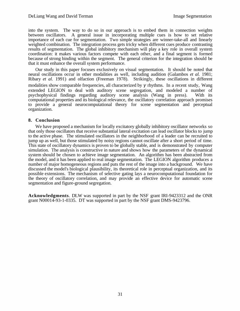
DeLiang Wang and David Terman Image Segmentation
31
into the system. The way to do so in our approach is to embed them in connection weightsbetween oscillators. A general issue in incorporating multiple cues is how to set relativeimportance of each cue for segmentation. Two simple strategies are winner-take-all and linearlyweighted combination. The integration process gets tricky when different cues produce contrastingresults of segmentation. The global inhibitory mechanism will play a key role in overall systemcoordination: it makes various factors compete with each other, and a final segment is formedbecause of strong binding within the segment. The general criterion for the integration should bethat it must enhance the overall system performance.
Our study in this paper focuses exclusively on visual segmentation. It should be noted thatneural oscillations occur in other modalities as well, including audition (Galambos et al. 1981;Ribary et al. 1991) and olfaction (Freeman 1978). Strikingly, these oscillations in differentmodalities show comparable frequencies, all characterized by γ rhythms. In a recent study, Wangextended LEGION to deal with auditory scene segregation, and modeled a number ofpsychophysical findings regarding auditory scene analysis (Wang in press). With itscomputational properties and its biological relevance, the oscillatory correlation approach promisesto provide a general neurocomputational theory for scene segmentation and perceptualorganization.
8. ConclusionWe have proposed a mechanism for locally excitatory globally inhibitory oscillator networks so
that only those oscillators that receive substantial lateral excitation can lead oscillator blocks to jumpto the active phase. The stimulated oscillators in the neighborhood of a leader can be recruited tojump up as well, but those stimulated by noisy regions cannot oscillate after a short period of time.This state of oscillatory dynamics is proven to be globally stable, and is demonstrated by computersimulation. The analysis is constructive in nature and shows how the parameters of the dynamicalsystem should be chosen to achieve image segmentation. An algorithm has been abstracted fromthe model, and it has been applied to real image segmentation. The LEGION algorithm produces anumber of major homogeneous regions and puts the rest of the image into a background. We havediscussed the model's biological plausibility, its theoretical role in perceptual organization, and itspossible extensions. The mechanism of selective gating lays a neurocomputational foundation forthe theory of oscillatory correlation, and may provide an effective device for automatic scenesegmentation and figure-ground segregation.
Acknowledgments. DLW was supported in part by the NSF grant IRI-9423312 and the ONRgrant N00014-93-1-0335. DT was supported in part by the NSF grant DMS-9423796.

DeLiang Wang and David Terman Image Segmentation
32
ReferencesAbeles, M. 1982. Local cortical circuits. Springer, New York. Abeles, M. 1991. Corticonics: Neural circuits of the cerebral cortex. Cambridge University Press,
New York. Adams, R., and Bischof, L. 1994. Seeded region growing. IEEE Trans. Pattern Anal. Machine
Intell. 16, 641-647.Anderson, J.A. 1995. An introduction to neural networks. MIT Press, Cambridge MA.Baldi, P., and Meir, R. 1990. Computing with arrays of coupled oscillators: An application to
preattentive texture discrimination. Neural Comp. 2, 458-471.Barlow, H. B. 1972. Single units and cognition: A neurone doctrine for perceptual psychology.
Percept. 1, 371-394.Biederman, I. 1987. Recognition-by-component: A theory of human image understanding.
Psychol. Rev. 94, 115-147.Bressler, S. L., Coppola, R., and Nakamura, R. 1993. Episodic multiregional cortical coherence
at multiple frequencies during visual task performance. Nature 366, 153-156.Buhmann, J. 1989. Oscillations and low firing rates in associative memory neural networks. Phys.
Rev. A 40, 4145-4148.Buzsáki, G., Llinás, R., Singer, W., Berthoz, A., and Christen, Y. (ed.). 1994. Temporal
coding in the brain. Springer-Verlag, Berlin Heidelberg.Crick, F. 1984. Function of the thalamic reticular complex: The searchlight hypothesis. Proc. Natl.
Acad. Sci. USA 81, 4586-4590.Crick, F. 1994. The astonishing hypothesis. Scribner, New York. Eckhorn, R., et al. 1988. Coherent oscillations: A mechanism of feature linking in the visual
cortex. Biol. Cybern. 60, 121-130.Engel, A. K., König, P., Kreiter, A. K., and Singer, W. 1991a. Interhemispheric synchronization
of oscillatory neuronal responses in cat visual cortex. Science 252, 1177-1179.Engel, A. K., König, P., Kreiter, A. K., and Singer, W. 1991b. Synchronization of oscillatory
neuronal responses between striate and extrastriate visual cortical areas of the cat. Proc. Natl.Acad. Sci. USA 88, 6048-6052.
FitzHugh, R. 1961. Impulses and physiological states in models of nerve membrane. Biophys. J.1, 445-466.
Foresti, G., Murino, V., Regazzoni, C. S., and Vernazza, G. 1994. Grouping of rectilinearsegments by the labeled Hough transform. CVGIP: Image Understanding 58(3), 22-42.
Freeman, W. J. 1978. Spatial properties of an EEG event in the olfactory bulb and cortex.Electroencephalogr. Clin. Neurophysiol. 44, 586-605.
Galambos, R., Makeig, S., and Talmachoff, P. J. 1981. A 40-Hz auditory potential recorded fromthe human scalp. Proc. Natl. Acad. Sci. USA 78, 2643-2647.
Geman, D., Geman, S., Graffigne, C., and Dong, P. 1990. Boundary detection by constrainedoptimization. IEEE Trans. Pattern Anal. Machine Intell. 12, 609-628.
Gilbert, C. D. 1992. Horizontal integration and cortical dynamics. Neuron 9, 1-13.Gilbert, C. D., Hirsch, J. A., and Wiesel, T. N. 1990. Lateral interactions in visual cortex. Cold
Spring Harbor Symposia on Quantitative Biology LV , 663-677.Gilbert, C. D., and Wiesel, T. N. 1989. Columnar specificity of intrinsic horizontal and
corticocortical connections in cat visual cortex. J. Neurosci. 9, 2432-2442.

DeLiang Wang and David Terman Image Segmentation
33
Goodhill, G. J., and Barrow, H. G. 1994. The role of weight normalization in competitivelearning. Neural Comp. 6, 255-269.
Gove, A., Grossberg, S., and Mingolla, E. in press. Brightness perception, illusory contours, andcorticogeniculate feedback. Visual Neurosci.
Gray, C. M., König, P., Engel, A. K., and Singer, W. 1989. Oscillatory responses in cat visualcortex exhibit inter-columnar synchronization which reflects global stimulus properties. Nature338, 334-337.
Grossberg, S., and Mingolla, E. 1985. Neural dynamics of perceptual grouping: Textures,boundaries, and emergent computations. Percept. Psychophys. 38, 141-171.
Grossberg, S., and Wyse, L. 1991. A neural network architecture for figure-ground separation ofconnected scenic figures. Neural Net. 4, 723-742.
Gurari, E. M., and Wechsler, H. 1982. On the difficulties involved in the segmentation ofpictures. IEEE Trans. Pattern Anal. Machine Intell. 4(3), 304-306.
Haralick, R. M. 1979. Statistical and structural approaches to texture. Proc. IEEE 67, 786-804.Haralick, R. M., and Shapiro, L. G. 1985. Image segmentation techniques. Comput. Graphics
Image Process. 29, 100-132.Hodgkin, A. L., and Huxley, A. F. 1952. A quantitative description of membrane current and its
application to conduction and excitation in nerve. J. Physiol. (Lond.) 117, 500-544.Horn, D., and Usher, M. 1991. Parallel activation of memories in an oscillatory neural network.
Neural Comp. 3, 31-44.Horowitz, S. L., and Pavlidis, T. 1976. Picture segmentation by a tree traversal algorithm. J.
ACM 23, 368-388.Hummel, J. E., and Biederman, I. 1992. Dynamic binding in a neural network for shape
recognition. Psychol. Rev. 99, 480-517.Kandel, E. R., Schwartz, J. H., and Jessell, T. M. 1991. Principles of neural science, 3rd ed.
Elsevier, New York. Koffka, K. 1935. Principles of Gestalt psychology. Harcourt, New York. Koh, J., Suk, M., and Bhandarkar, S. M. 1995. A multilayer self-organizing feature map for
range image segmentation. Neural Net. 8, 67-86.Kohler, R. 1981. A segmentation system based on thresholding. Comput. Graphics Image
Process. 15, 319-338.Kohonen, T. 1995. Self-organizing maps. Springer, Berlin Heidelberg. Lamme, V. A. F., van Dijk, B. W., and Spekreijse, H. 1993. Coutour from motion processing
occurs in primary visual cortex. Nature 363, 541-543.Liberman, A. M., Isenberg, D., and Rakerd, B. 1981. Duplex percepton of cues for stop
consonants: Evidence for a phonetic mode. Percept. Psychophys. 30, 133-143.Liou, S. P., Chiu, A. H., and Jain, R. C. 1991. A parallel technique for signal-level perceptual
organization. IEEE Trans. Pattern Anal. Machine Intell. 13, 317-325.LoFaro, T. 1994. A period adding bifurcation in a pair of coupled neurons. Ph.D dissertation,
Boston University.Lowe, D. G. 1985. Perceptual organization and visual recognition. Kluwer Academic, Boston
MA. Manjunath, B. S., and Chellappa, R. 1993. A unified approach to boundary perception: Edges,
textures, and illusory contours. IEEE Trans. Neural Net. 4, 96-108.Marr, D. 1982. Vision. Freeman, New York.
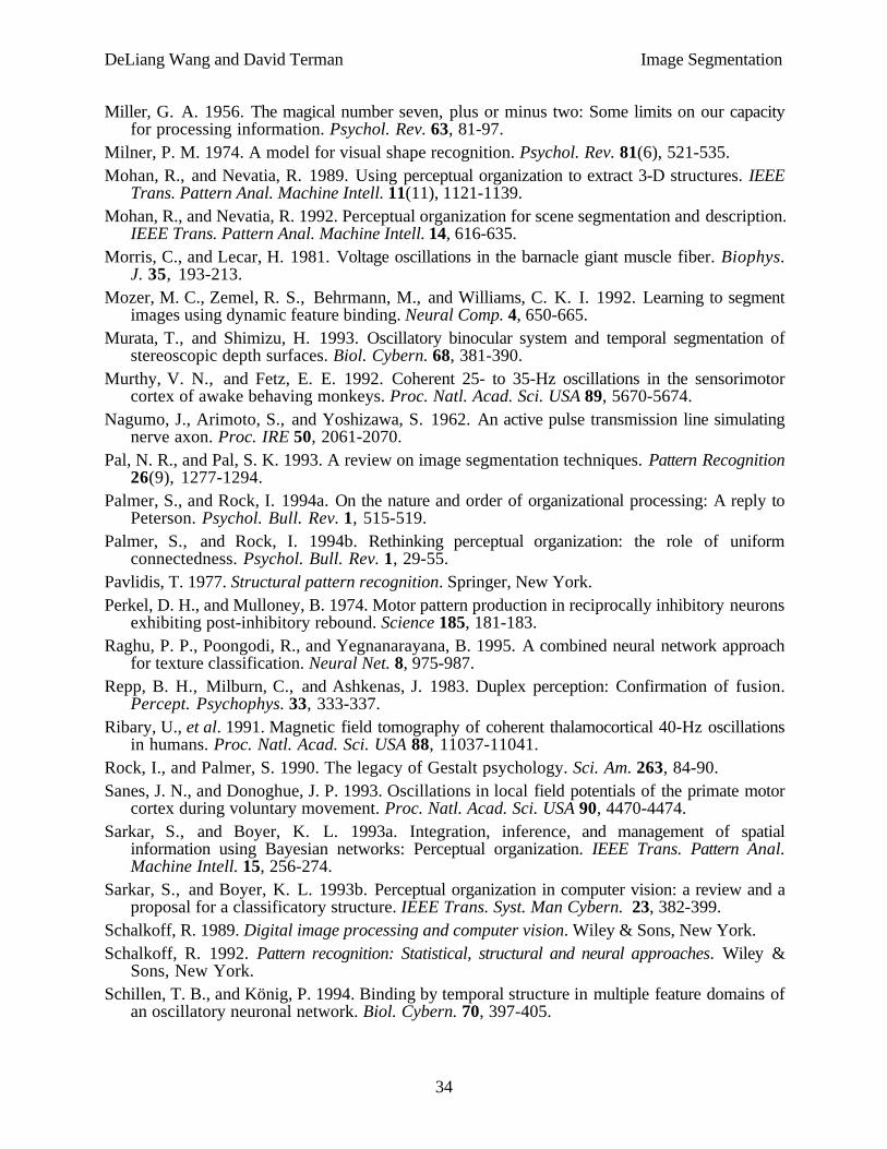
DeLiang Wang and David Terman Image Segmentation
34
Miller, G. A. 1956. The magical number seven, plus or minus two: Some limits on our capacityfor processing information. Psychol. Rev. 63, 81-97.
Milner, P. M. 1974. A model for visual shape recognition. Psychol. Rev. 81(6), 521-535.Mohan, R., and Nevatia, R. 1989. Using perceptual organization to extract 3-D structures. IEEE
Trans. Pattern Anal. Machine Intell. 11(11), 1121-1139.Mohan, R., and Nevatia, R. 1992. Perceptual organization for scene segmentation and description.
IEEE Trans. Pattern Anal. Machine Intell. 14, 616-635.Morris, C., and Lecar, H. 1981. Voltage oscillations in the barnacle giant muscle fiber. Biophys.
J. 35, 193-213.Mozer, M. C., Zemel, R. S., Behrmann, M., and Williams, C. K. I. 1992. Learning to segment
images using dynamic feature binding. Neural Comp. 4, 650-665.Murata, T., and Shimizu, H. 1993. Oscillatory binocular system and temporal segmentation of
stereoscopic depth surfaces. Biol. Cybern. 68, 381-390.Murthy, V. N., and Fetz, E. E. 1992. Coherent 25- to 35-Hz oscillations in the sensorimotor
cortex of awake behaving monkeys. Proc. Natl. Acad. Sci. USA 89, 5670-5674.Nagumo, J., Arimoto, S., and Yoshizawa, S. 1962. An active pulse transmission line simulating
nerve axon. Proc. IRE 50, 2061-2070.Pal, N. R., and Pal, S. K. 1993. A review on image segmentation techniques. Pattern Recognition
26(9), 1277-1294.Palmer, S., and Rock, I. 1994a. On the nature and order of organizational processing: A reply to
Peterson. Psychol. Bull. Rev. 1, 515-519.Palmer, S., and Rock, I. 1994b. Rethinking perceptual organization: the role of uniform
connectedness. Psychol. Bull. Rev. 1, 29-55.Pavlidis, T. 1977. Structural pattern recognition. Springer, New York. Perkel, D. H., and Mulloney, B. 1974. Motor pattern production in reciprocally inhibitory neurons
exhibiting post-inhibitory rebound. Science 185, 181-183.Raghu, P. P., Poongodi, R., and Yegnanarayana, B. 1995. A combined neural network approach
for texture classification. Neural Net. 8, 975-987.Repp, B. H., Milburn, C., and Ashkenas, J. 1983. Duplex perception: Confirmation of fusion.
Percept. Psychophys. 33, 333-337.Ribary, U., et al. 1991. Magnetic field tomography of coherent thalamocortical 40-Hz oscillations
in humans. Proc. Natl. Acad. Sci. USA 88, 11037-11041.Rock, I., and Palmer, S. 1990. The legacy of Gestalt psychology. Sci. Am. 263, 84-90.Sanes, J. N., and Donoghue, J. P. 1993. Oscillations in local field potentials of the primate motor
cortex during voluntary movement. Proc. Natl. Acad. Sci. USA 90, 4470-4474.Sarkar, S., and Boyer, K. L. 1993a. Integration, inference, and management of spatial
information using Bayesian networks: Perceptual organization. IEEE Trans. Pattern Anal.Machine Intell. 15, 256-274.
Sarkar, S., and Boyer, K. L. 1993b. Perceptual organization in computer vision: a review and aproposal for a classificatory structure. IEEE Trans. Syst. Man Cybern. 23, 382-399.
Schalkoff, R. 1989. Digital image processing and computer vision. Wiley & Sons, New York. Schalkoff, R. 1992. Pattern recognition: Statistical, structural and neural approaches. Wiley &
Sons, New York. Schillen, T. B., and König, P. 1994. Binding by temporal structure in multiple feature domains of
an oscillatory neuronal network. Biol. Cybern. 70, 397-405.

DeLiang Wang and David Terman Image Segmentation
35
Sejnowski, T. J., and Hinton, G. E. 1987. Separating figure from ground with a Boltzmannmachine. In Vision, brain, and cooperative computation, M. A. Arbib, and A. R. Hanson, ed.,pp. 703-724. MIT Press, Cambridge MA.
Sha'ashua, A., and Ullman, S. 1988. Structural saliency: The detection of globally salientstructures using a locally connected network. In Proc. Int. Conf. Comput. Vision, pp. 321-327.
Sillito, A. M., Jones, H. E., Gerstein, G. L., and West, D. C. 1994. Feature-linkedsynchronization of thalamic relay cell firing induced by feedback from the visual cortex. Nature369, 479-482.
Singer, W. 1993. Synchronization of cortical activity and its putative role in informationprocessing and learning. Ann. Rev. Physiol. 55, 349-374.
Singer, W., and Gray, C. M. 1995. Visual feature integration and the temporal correlationhypothesis. Ann. Rev. Neursci. 18, 555-586.
Somers, D., and Kopell, N. 1993. Rapid synchrony through fast threshold modulation. Biol.Cybern. 68, 393-407.
Somers, D., and Kopell, N. in press. Waves and synchrony in networks of oscillators ofrelaxation and non-relaxation type. Physica D.
Sompolinsky, H., Golomb, D., and Kleinfeld, D. 1991. Cooperative dynamics in visualprocessing. Phys. Rev. A 43, 6990-7011.
Sompolinsky, H., and Tsodyks, M. 1994. Segmentation by a network of oscillators with storedmemories. Neural Comp. 6(4), 642-657.
Sporns, O., Gally, J. A., Reeke Jr., G. N., and Edelman, G. M. 1989. Reentrant signalingamong simulated neuronal groups leads to coherency in their oscillatory activity. Proc. Natl.Acad. Sci. USA 86, 7265-7269.
Sporns, O., Tononi, G., and Edelman, G. M. 1991. Modeling perceptual grouping and figure-ground segregation by means of active re-entrant connections. Proc. Natl. Acad. Sci. USA 88,129-133.
Stoner, G. R., and Albright, T. D. 1992. Neural correlates of perceptual motion coherence. Nature358, 412-414.
Terman, D., and Wang, D. L. 1995. Global competition and local cooperation in a network ofneural oscillators. Physica D 81, 148-176.
Uchiyama, T., and Arbib, M. A. 1994. Color image segmentation using competitive learning.IEEE Trans. Pattern Anal. Machine Intell. 16(12), 1197-1206.
von der Malsburg, C. 1973. Self-organization of orientation sensitive cells in the striate cortex.Kybernetik 14, 85-100.
von der Malsburg, C. 1981. The correlation theory of brain function. Internal Report 81-2, Max-Planck-Institute for Biophysical Chemistry.
von der Malsburg, C., and Buhmann, J. 1992. Sensory segmentation with coupled neuraloscillators. Biol. Cybern. 54, 29-40.
von der Malsburg, C., and Schneider, W. 1986. A neural cocktail-party processor. Biol. Cybern.54, 29-40.
Wang, D. L. 1993a. Modeling global synchrony in the visual cortex by locally coupled neuraloscillators. In Proc. of 15th Ann. Conf. Cognit. Sci. Soc., pp. 1058-1063. Boulder CO.
Wang, D. L. 1993b. Pattern recognition: Neural networks in perspective. IEEE Expert 8, 52-60,August.
Wang, D. L. 1995. Emergent synchrony in locally coupled neural oscillators. IEEE Trans. NeuralNet. 6(4), 941-948.

DeLiang Wang and David Terman Image Segmentation
36
Wang, D. L. in press. Primitive auditory segregation based on oscillatory correlation. Cognit. Sci.Wang, D. L., Buhmann, J., and Malsburg, C. v. d. 1990. Pattern segmentation in associative
memory. Neural Comp. 2, 95-107. Reprinted in Olfaction, J.L. Davis and H. Eichenbaum,ed. Cambridge MA: MIT Press, pp. 213-224, 1991.
Wang, D. L., and Terman, D. 1995. Locally excitatory globally inhibitory oscillator networks.IEEE Trans. Neural Net. 6(1), 283-286.
Wang, D. L., and Yuwono, B. 1995. Anticipation-based temporal pattern generation. IEEE Trans.Syst. Man Cybern. 25, 615-628.
Watt, R. J. 1987. Scanning from coarse to fine spatial scales in the human visual system after theonset of a stimulus. J. Opt. Soc. Am. A4, 2006-2021.
Wertheimer, M. 1923. Untersuchungen zur Lehre von der Gestalt, II. Psychol. Forsch. 4, 301-350.
Whittington, M. A., Traub, R. D., and Jefferys, J. G. R. 1995. Synchronized oscillations ininterneuron networks driven by metabotropic glutamate receptor activation. Nature 373, 612-615.
Zeki, S. 1993. A vision of the brain. Blackwell Scientific, Oxford, England. Zucker, S. W. 1976. Region growing: Childhood and adolescence. Comput. Graphics Image
Process. 5, 382-399.

DeLiang Wang and David Terman Image Segmentation
37
Figure CaptionFigure 1. A caricature of an image with three objects that appear on a noisy background. The
noiseless caricature is adapted from (Terman and Wang 1995).Figure 2. Nullclines and orbits of a single oscillator (We thank S. Campbell for making this
figure). A . If I > 0 and H = 1, the oscillator is enabled. The periodic orbit is shown with abold curve, and its direction of motion is indicated by the arrowheads. The left and the rightbranches of the x-nullcline are labeled as L and R , respectively. LK and RK indicate the leftand the right knees of the cubic, respectively. B. If I ≤ 0 and H = 1, the oscillator is excitable.The fixed point PI on the left branch of the cubic is asymptotically stable.
Figure 3. Architecture of a two dimensional LEGION network with four nearest-neighborcoupling. An oscillator is indicated by an open circle, and the global inhibitor is indicated bythe filled circle.
Figure 4. The effects of two neighborhoods. N1(i) is the potential neighborhood, and N2(i) isthe coupling neighborhood.
Figure 5. A An image composed of four patterns which are presented to a 25x25 LEGIONnetwork (adapted from Wang and Terman 1995). Each square corresponds to an oscillator.Filled squares indicate stimulated oscillators, while open squares indicate unstimulatedoscillators. B The image in A is corrupted by 10% noise. C A snapshot of the activities of thenetwork at the beginning of dynamic evolution. D Another snapshot taken shortly after C. EAnother snapshot taken shortly after D. F Another snapshot taken shortly after E. G Anothersnapshot taken shortly after F.
Figure 6. Temporal evolution of every stimulated oscillator. The upper four traces show thecombined temporal activities of the four oscillator blocks representing the four correspondingpatterns indicated by their respective labels. The fifth trace shows the temporal activities of theloners corresponding to the background, and the bottom trace shows the activity of the globalinhibitor. The ordinates except for the bottom one in the figure indicate the normalized x-activity of an oscillator, and the inhibitor trace is drawn according to the normalized activity.The simulation took 8,000 integration steps.
Figure 7. Another simulation with an alternative definition for a single oscillator. See the legendof Fig. 6 for explanations. As in Fig. 6, this simulation took 8,000 integration steps.
Figure 8. A An image composed of nine patterns which are presented to a 30x30 LEGIONnetwork. See the legend of Fig. 5 for explanations. B A snapshot of network activity at thebeginning of dynamic evolution. C Another snapshot taken shortly after B . D Anothersnapshot taken shortly after C. E Another snapshot taken shortly after D. F Another snapshottaken shortly after E. G Another snapshot taken shortly after F.
Figure 9. Temporal evolution of every stimulated oscillator. The upper nine traces show thecombined temporal activities of the oscillator blocks representing the nine correspondingpatterns indicated by their respective labels. The bottom trace shows the activity of the globalinhibitor. See the legend of Fig. 6 for further explanations. The simulation took 8,000integration steps.
Figure 10. A scenario for producing overlapping segments. A square indicates a pixel with itsvalue shown in the middle.
Figure 11. A: A gray-level image consisting of 160x160 pixels (by courtesy of K. Boyer). Theimage is presented to a 160x160 LEGION network. B One segment pops out from thenetwork shortly after the LEGION algorithm is executed. C Another segment pops out shortlyafter B. D Another segment pops out shortly after C. E Another segment popped out shortlyafter D. F Another segment pops out shortly after E. G Another segment pops out shortlyafter F. (We thank E. Cesmeli for his assistance in making this figure)

DeLiang Wang and David Terman Image Segmentation
38
Figure 12: A gray map showing the result of segmenting Fig. 11A. The algorithm produces 16segments plus a background. The algorithm was run for 1,000 time steps.
Figure 13. A gray map showing the result of segmenting Fig. 11A. Maximization is used tocompute Si. The algorithm produces 17 segments plus a background. The algorithm was runfor 1,000 steps.
Figure 14. Comparison between summation and maximization in computing Si. A and B showtwo different scenarios.
Figure 15. A gray map showing the result of segmenting Fig. 11A with a different value for θp.The system produces 23 segments plus a background. The algorithm was run for 1,000 steps.
Figure 16. A A gray-level image consisting of 256x256 pixels (by courtesy of N. Shareef). B Agray map showing the result of segmenting the image in A by a 256x256 LEGION network.The system produces 21 segments plus a background. C A gray map showing the result ofsegmenting the image in A with different values of Wz and θp. The system produces 25segments plus a background. The algorithm was run for 1,200 steps in both B and C.
Figure 17. A A gray-level image consisting of 256x256 pixels (by courtesy of N. Shareef). B Agray map showing the result of segmenting the image in A by a 256x256 LEGION network.The system produces 17 segments plus a background. C A gray map showing the result ofsegmenting the image in A with different values of Wz and θp. The system produces 13segments plus a background. The algorithm was run for 1,200 steps in both B and C.

DeLiang Wang and David Terman Image Segmentation
39
Figure 1

DeLiang Wang and David Terman Image Segmentation
40
H
x
y
C
PI
B
x
RL
RK
LK
A
H:y' 0=C:x' 0=
y
Figure 2
DeLiang Wang and David Terman Image Segmentation
41
......
...
...
............
............
......
Global Inhibitor
Figure 3

DeLiang Wang and David Terman Image Segmentation
42
N1(i) N2(i)
Figure 4

DeLiang Wang and David Terman Image Segmentation
43
A B C
D E F
G
Figure 5

DeLiang Wang and David Terman Image Segmentation
44
Left O
Pattern H
Pattern I
Right O
Background
Inhibitor
Time
Figure 6

DeLiang Wang and David Terman Image Segmentation
45
Left O
Pattern H
Pattern I
Right O
Background
Inhibitor
Time
Figure 7
DeLiang Wang and David Terman Image Segmentation
46
A B C
D E F
G
Figure 8

DeLiang Wang and David Terman Image Segmentation
47
Left O
Pattern H
Pattern I
Right O
Pattern S
Left T
Pattern A
Right T
Pattern E
Inhibitor
Time
Figure 9

DeLiang Wang and David Terman Image Segmentation
48
AAAAA50AAAAAA
30
AAAAAAA50
AAAAAA50AAAAAA
30
AAAA30
AAAA30AAAA30AA
AAAA
30
AAAA30AAAA30AAAAAAAAA
30
AAAAAA30
Figure 10

DeLiang Wang and David Terman Image Segmentation
49
A
B C D
E F G
Figure 11

DeLiang Wang and David Terman Image Segmentation
50
Figure 12

DeLiang Wang and David Terman Image Segmentation
51
Figure 13

DeLiang Wang and David Terman Image Segmentation
52
AAAAAAAA30
AAAAAAAA50
AAAAAA40
AAAAAA50
A B
Summation
Maximum groupingno grouping
BA
grouping no grouping
AAAAAAAA30
AAAAAAAA30
AAAAAAAA30
AAAAAA30AA
AAAA30AA
AAAAA30
AAAAAAAAAA30
Figure 14

DeLiang Wang and David Terman Image Segmentation
53
Figure 15

DeLiang Wang and David Terman Image Segmentation
54
A
B C
Figure 16

DeLiang Wang and David Terman Image Segmentation
55
A
B C
Figure 17