Embed Size (px)
Citation preview

Image SamplingImage SamplingImage SamplingImage Sampling

ExampleExampleExampleExample

Matrix RepresentationMatrix RepresentationMatrix RepresentationMatrix Representation

A QuantizerA QuantizerA QuantizerA Quantizer

Matrix RepresentationMatrix RepresentationMatrix RepresentationMatrix Representation

Uniform QuantizationUniform QuantizationUniform QuantizationUniform Quantization

A Uniform QuantizerA Uniform QuantizerA Uniform QuantizerA Uniform Quantizer

Example 1 of Uniform QuantizerExample 1 of Uniform Quantizer

Example 2 of Uniform Example 2 of Uniform Example 2 of Uniform Quantizer
Example 2 of Uniform Quantizer

Q i i Q i i Quantization Effect – False Quantization Effect – False Effect False
ContourEffect False
Contour

Examples of Uniform Examples of Uniform Examples of Uniform Quantizer
Examples of Uniform Quantizer

Ch t 2 Di it l I F d t lCh t 2 Di it l I F d t lChapter 2: Digital Image FundamentalsChapter 2: Digital Image Fundamentals

Ch t 2 Di it l I F d t lCh t 2 Di it l I F d t lChapter 2: Digital Image FundamentalsChapter 2: Digital Image Fundamentals

Ch t 2 Di it l I F d t lCh t 2 Di it l I F d t lChapter 2: Digital Image FundamentalsChapter 2: Digital Image Fundamentals

Ch t 2 Di it l I F d t lCh t 2 Di it l I F d t lChapter 2: Digital Image FundamentalsChapter 2: Digital Image Fundamentals

Chapter 2: Digital Image FundamentalsChapter 2: Digital Image Fundamentalsp g gp g g

Ch t 2 Di it l I F d t lCh t 2 Di it l I F d t lChapter 2: Digital Image FundamentalsChapter 2: Digital Image Fundamentals

Ch t 2 Di it l I F d t lCh t 2 Di it l I F d t lChapter 2: Digital Image FundamentalsChapter 2: Digital Image Fundamentals

Ch t 2 Di it l I F d t lCh t 2 Di it l I F d t lChapter 2: Digital Image FundamentalsChapter 2: Digital Image Fundamentals

Chapter 3Chapter 3Image Enhancement in the
Spatial DomainImage Enhancement in the
Spatial Domain
The principal objective of enhancement is to process an image so that the result image is more suitable than the original image for a specific application. There are two broad categories:categories:
•Spatial domain: These approaches are based on direct p ppmanipulation of pixels in an image.•Frequency domain: These techniques are based on
d f h f fmodifying the Fourier transform of an image.

Chapter 3Chapter 3Image Enhancement in the
Spatial DomainImage Enhancement in the
Spatial Domain
Spatial domain refers to the aggregate of pixels composing an image. Spatial domain methods are procedures that operate directly on these pixels.p

Chapter 3Chapter 3Image Enhancement in the
Spatial DomainImage Enhancement in the
Spatial Domain
Contrast Stretching Thresholding Function

Chapter 3Chapter 3Point Processing and mask processing
or filteringPoint Processing and mask processing
or filtering

Chapter 3Chapter 3Image Enhancement in the
Spatial DomainImage Enhancement in the
Spatial Domain
Wh i C hi ?What is Contrast stretching?

Chapter 3Chapter 3Image Enhancement in the
Spatial DomainImage Enhancement in the
Spatial Domain
H h h ?How to enhance the contrast?
Low contrast image values concentrated near anarrow range (mostly dark, or mostly bright, or mostly
di l )medium values)• Contrast enhancement change the image valuedistribution to cover a wide rangedistribution to cover a wide range• Contrast of an image can be revealed by its histogram

Chapter 3Chapter 3Some Basic Gray Level TransformSome Basic Gray Level Transform
- Image Negatives
- Log Transformations
- Power-Law Transformations

Chapter 3Chapter 3Image NegativesImage Negatives
Image Negatives

Chapter 3Chapter 3Log TransformationsLog Transformations
Log Transformations

Chapter 3Chapter 3Power-Law TransformationsPower-Law Transformations
Power-LawPower Law Transformations
The exponent in the l tipower-law equation
is referred to as “gamma”gamma

Chapter 3Chapter 3Gamma CorrectionGamma Correction

Chapter 3Chapter 3Power-Law TransformationsPower-Law Transformations

Chapter 3Chapter 3Power-Law TransformationsPower-Law Transformations

Chapter 3Chapter 3Log /Power-Law TransformationsLog /Power-Law Transformations
f

Chapter 3Chapter 3Piecewise Linear StretchingPiecewise Linear Stretching

Chapter 3Chapter 3Contrast StretchingContrast Stretching

Chapter 3Chapter 3Gray-level SlicingGray-level Slicing

Chapter 3Chapter 3Gray-level SlicingGray-level Slicing
G l lGray-level slicing

Chapter 3Chapter 3Gray-level SlicingGray-level Slicing

Chapter 3Chapter 3Image Enhancement in the
Spatial DomainImage Enhancement in the
Spatial Domain
Chapter 3Chapter 3Image Enhancement in the
Spatial DomainImage Enhancement in the
Spatial Domain

Chapter 3Chapter 3Image Enhancement in the
Spatial DomainImage Enhancement in the
Spatial Domain

Review: Probability and Random VariablesReview: Probability and Random Variables
Random VariablesRandom Variables
Random Variable (RV)*Th S f ll ibl f i l– The set, S, of all possible outcomes of a particular
experiment is called the sample space for the iexperiment.
– An event is any collection of possible outcomes of i h i b f San experiment, that is, any subset of S.
– Random variable, x is a function from a sample S i h l bspace S into the real numbers.

Review: Probability and Random VariablesReview: Probability and Random Variables
Random Variables (Con’t)Random Variables (Con’t)
Examples of Random VariablesTossing two coins, X is the number of heads, and Y is the g , f ,number of tails
– X and Y take on values {0, 1, 2}– Discrete type
• X is the lifetime of a certain band of light bulbsX take on values [0 +∞)– X take on values [0, +∞)
– Continuous type• X is the intensity value (Gray level, 0-255) of pixels in an y ( y , ) f pimage
– X take on the values {0, 1, …, 255}i– Discrete type

Review: Probability and Random VariablesReview: Probability and Random Variables
Random Variables (Con’t)Random Variables (Con’t)
Di t ib ti D it d M F tiDistribution, Density, and Mass Functions

Review: Probability and Random VariablesReview: Probability and Random Variables
Random Variables (Con’t)Random Variables (Con’t)
S i l CSpecial Cases

Review: Probability and Random VariablesReview: Probability and Random Variables
Random Variables (Con’t)Random Variables (Con’t)
In Sec. 3.3 of the book we used the notation p(rk), k = 0,1,…, L - 1, to denote the histogram of an image with L possible gray levels rkto denote the histogram of an image with L possible gray levels, rk, k = 0,1,…, L - 1, where p(rk) is the probability of the kth gray level (random event) occurring. The discrete random variables in this case are gray levels. It generally is clear from the context whether one is working with continuous or discrete random variables, and
h th th f b i ti i f l it Alwhether the use of subscripting is necessary for clarity. Also, uppercase letters (e.g., P) are frequently used to distinguish between probabilities and probability density functions (e g p)between probabilities and probability density functions (e.g., p) when they are used together in the same discussion.

Review: Probability and Random VariablesReview: Probability and Random Variables
Random Variables (Con’t)Random Variables (Con’t)
If a random variable x is transformed by a monotonic transformation function T(x) to produce a new random variable y, h b bili d i f i f b b i d fthe probability density function of y can be obtained from
knowledge of T(x) and the probability density function of x, as follows:follows:
where the subscripts on the p's are used to denote the fact that they are different functions, and the vertical bars signify the b l l A f i T( ) i i ll i i ifabsolute value. A function T(x) is monotonically increasing if
T(x1) < T(x2) for x1 < x2, and monotonically decreasing if T(x1) > T(x ) for x < x The preceding equation is valid if T(x) is an> T(x2) for x1 < x2. The preceding equation is valid if T(x) is an increasing or decreasing monotonic function.

Chapter 3Chapter 3Histogram ProcessingHistogram Processing
h i hi f i ?What is a histogram of an image?
I = imread('pout tif');I = imread( pout.tif );imshow(I);figure, imhist(I,64);g , ( , );

Chapter 3Chapter 3Histogram ProcessingHistogram Processing
Dark imageC ll Dark imageThe components of the histogram are concentrated on the low side
f th l
Can we tell something b h of the gray scale.
Bright imageThe components of the histogram
about the image,f j The components of the histogram
biased toward the high side of the gray scale.
from just look at its hi ? Low Contrast image
The histogram will be narrow and will be concentrated on toward the
histogram?
middle of the gray scale.High Contrast imagewhose pixels have a large variety of graylarge variety of gray tones. The histogram is not far from a uniform.

Chapter 3Chapter 3Histogram ProcessingHistogram Processing
Different images But have the same histogramDifferent images But have the same histogram

Chapter 3Chapter 3Histogram ProcessingHistogram Processing
More examples of histograms

Chapter 3Chapter 3Histogram ProcessingHistogram Processing
Histogram CalculationHistogram Calculation

Chapter 3Chapter 3Contrast StretchingContrast Stretching

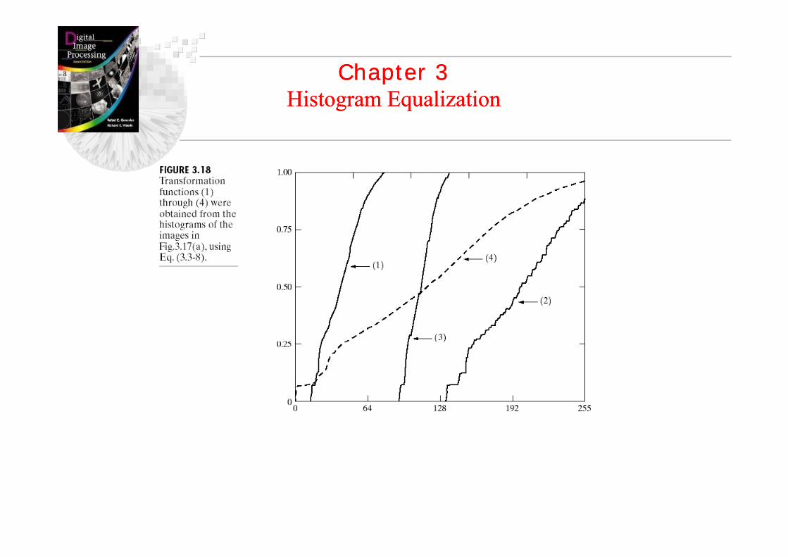
Chapter 3Chapter 3Histogram EqualizationHistogram Equalization
r is a gray level normalized to the interval [0, 1] which r = 0 representing black and r = 1 representing whitewhich r 0 representing black and r 1 representing white
S=T(r) 0 ≤ r ≤ 1The transformation function T(r) satisfies the following conditions:The transformation function T(r) satisfies the following conditions:(a) T(r) is single-valued and monotonically incresing in the interval0 ≤ r ≤ 1 and(b) 0 ≤ T( ) ≤ 1 f 0 ≤ ≤ 1(b) 0 ≤ T(r) ≤ 1 for 0 ≤ r ≤ 1

Chapter 3Chapter 3Chapter 3Histogram Equalization
Chapter 3Histogram Equalization
Transform an image with an arbitrary histogram to another image ith a flat histogramanother image with a flat histogram.
• Suppose r has pdf, pr(r) where 0 ≤ r ≤ 0
• Use the transformation
• s has a uniform pdf in (0 1)• s has a uniform pdf in (0,1)

Chapter 3Chapter 3Histogram EqualizationHistogram Equalization
Need and output histogram (distribution)Need and output histogram (distribution)to be uniform or flat.
A f d t l lt f b i b bilitA fundamental result from basic porbabilitytheory is that if pr(r) and T(r) are know, and T(r) is continuous and differentiable, the
h f f d i bl bThe PDF of transformed variable s can beObtained using
ps(s)ds = pr(r)dr or

Chapter 3Chapter 3
In the case of histogram:
Histogram EqualizationHistogram Equalization
e c se o s og :)()()1()(
0
wdwpLsTsr
r∫−==
Where (L-1) is the maximum intensity value of an image.
dTd )(dr
rdTdrds )(
=
⎥⎤
⎢⎡
−= ∫r
r wdwpddL )()()1( ⎥
⎦⎢⎣∫ rp
ds 0
)()()(
)()1( rpL r−=ds
Substitutes in the equationdrds
)()1(1)()()(
rpLrp
drdsrpsp rrs == 1)( =sps)()1( rpLdr r−
)1(1−
=L
10 −≤≤ Ls)1(
)(−L
ps

Chapter 3Chapter 3Histogram EqualizationHistogram Equalization
1)1(
1)(−
=L
sps
From the example ps(s) is a uniform PDF. Note that T(r)depends on pr(r) but as shows, the resultin ps(s) always isdepends on pr(r) but as shows, the resultin ps(s) always is uniform, independently of the form of ps(s) .

Chapter 3Chapter 3Chapter 3Histogram Equalization
Chapter 3Histogram Equalization

Chapter 3Chapter 3pHistogram Equalization
pHistogram Equalization
Ex: Suppose that a 3-bit image (L=8) of size 64x64 (4096 pixels) has the intensity distribution shown in table.
1 33 11.33 → 13.08 → 34.55 → 54.55 55.67 → 66.23 → 66.65 → 76.86 → 77 00 77.00 → 7

Chapter 3Chapter 3Chapter 3Histogram Equalization
Chapter 3Histogram Equalization

Chapter 3Chapter 3Histogram EqualizationHistogram Equalization
ExampleExample
rk pr(rk) sk = 7* sk ps(sk)0 0.19 0.19 [1.33]=11 0.25 0.44 [3.08]=3
0 0
1 0.191 0.25 0.44 [3.08] 32 0.21 0.65 [4.55]=53 0 16 0 81 [5 67] 6
12 0
3 0 253 0.16 0.81 [5.67]=64 0.08 0.89 [6.03]=6
3 0.25
4 0
5 0.06 0.95 [6.65]=76 0.03 0.98 [6.86]=7
5 0.21
6 0.16+0. = 0.0.246 0.03 0.98 [6.86] 77 0.02 1.00 [7]=7
67 0.06+0.03+0.02=0.11

Chapter 3Chapter 3Histogram EqualizationHistogram Equalization
ExampleExampleIntensity (rk)
No. of Pixels(nj)
sk = 7* sk
0 20 0.2 0.2x7 = 1.4 1
1 5 0.25 0.25*7 = 1.75 2
2 25 0.5 0.5*7 = 3.5 3
3 10 0.6 0.6*7 = 4.2 4
4 15 0.75 0.75*7 = 5.25 5
5 5 0.8 0.8*7 = 5.6 6
6 10 0.9 0.9*7 = 6.3 6
7 10 1.0 1.0x7 = 7 7
Total 100

Chapter 3Chapter 3Histogram EqualizationHistogram Equalization
Chapter 3Chapter 3Histogram EqualizationHistogram Equalization

Chapter 3Chapter 3Chapter 3Histogram Equalization
Chapter 3Histogram Equalization
Hi li i i l f i h i i l h hHistogram equalization involves transforming the intensity values so that the histogram of the output image approximately matches a specified histogram. (By default, histeq tries to match a uniform histogram with 64 bins, but you can specify a different histogram instead.)
I = imread('pout.tif');i h (I)imshow(I);[J,T] = histeq(I);figure;imshow(J);figure;imshow(J);figure, imhist(J,64);figure,plot((0:255)/255,T);

Chapter 3Chapter 3Histogram EqualizationHistogram Equalization

Chapter 3Chapter 3Histogram EqualizationSample Matlab Code
Histogram EqualizationSample Matlab Code

Chapter 3Chapter 3Chapter 3Project 1Chapter 3Project 1
N t ll i b tl t d i t f d d b k d i i lNot all images can be neatly segmented into foreground and background using simple thresholding. Whether or not an image can be correctly segmented this way can be determined by looking at an intensity histogram of the image.
If it is possible to separate out the foreground of an image on the basis of pixel intensity, then the intensity of pixels within foreground objects must be distinctly different from the intensity of pixels within the background. In this case, we expect to see a distinct peak in the histogram corresponding to foreground objects such that thresholds can be chosen to isolate this peak accordingly. If such a peak does not exist, then it is unlikely that simple thresholding will produce a good segmentation. In this case, adaptive thresholding may be a better answer.

Chapter 3Chapter 3Chapter 3Project 1Chapter 3Project 1
P j t 1Project 1

Chapter 3Chapter 3Histogram SpecificationHistogram Specification
zk=G-1[T(rk)]zk G [T(rk)]zk = G-1(sk)
k = 0, 1, 2,,…,L-1

Chapter 3Chapter 3Specific pdfHistogram SpecificationHistogram Specification
’
Calculate from a given imageSpecific pdf
rk pr(rk) pz(zk) zk p’z(zk)
0 0.19 0.19 0.0 0.0 0 0.01 0 25 0 44 0 0 0 0 1 0 01 0.25 0.44 0.0 0.0 1 0.02 0.21 0.65 0.0 0.0 2 0.03 0 16 0 81 0 15 0 15 3 0 193 0.16 0.81 0.15 0.15 3 0.194 0.08 0.89 0.35 0.20 4 0.255 0.06 0.95 0.65 0.30 5 0.216 0.03 0.98 0.85 0.20 6 0.247 0.02 1.00 1.00 0.15 7 0.11
rk 0 1 2 3 4 5 6 7
zk 3 4 5 6 6 7 7 7

Chapter 3Chapter 3Histogram SpecificationHistogram Specification
Histogram ของ input image เปนดังนี้ตองการให Histogramของ output image เปนดังนี้
Intensity( s )
# pixels
Histogram ของ input image เปนดงนIntensity ( z )
# pixels
ของ output image เปนดงน
โจทยตัวอยาง ( s )0 20
1 5
( )0 5
1 101 5
2 25
3 10
2 15
3 20
User เปนผูกําหนดขอมูลตั้งตน
3 10
4 15
5 5
4 20
5 155 5
6 10
7 10
6 10
7 57 10
Total 100 Total 100

Chapter 3Chapter 3Histogram SpecificationHistogram Specification
1. ทํา Histogram Equalization ทัง้สองตาราง
rk (nj) Σpr sk
0 20 0 2 1
zk (nj) Σpz vk
0 5 0 05 00 20 0.2 1
1 5 0.25 2
2 25 0 5 3
0 5 0.05 0
1 10 0.15 1
2 15 0 3 22 25 0.5 3
3 10 0.6 4
4 15 0 75 5
2 15 0.3 2
3 20 0.5 4
4 20 0 7 54 15 0.75 5
5 5 0.8 6
4 20 0.7 5
5 15 0.85 6
6 10 0.9 6
7 10 1.0 7
6 10 0.95 7
7 5 1.0 7
sk = T(rk) vk = G(zk)

Chapter 3Chapter 3Histogram SpecificationHistogram Specification
2. ไดตาราง Mapไดเปน
Actual Output Hi t
rk sk vk zk
rk sk vk zk
sk vk
ไดเปน
rk zk zk # Pixels
Histogram
0 1
1 2
0 0
1 1
0 1
1 2
0 0
1 20
2 3
3 4
2 2
4 3
2 2
3 3
2 30
3 10
4 5
5 6
5 4
6 5
4 4
5 5
4 15
5 15
6 6
7 7
7 6
7 7
6 5
7 6
6 10
7 07 7 7 7
sk = T(rk) zk = G-1(vk)

Chapter 3Chapter 3Image Enhancement in the
Spatial DomainImage Enhancement in the
Spatial Domain

Chapter 3Chapter 3Image Enhancement in the
Spatial DomainImage Enhancement in the
Spatial Domain

Chapter 3Chapter 3Image Enhancement in the
Spatial DomainImage Enhancement in the
Spatial Domain

Chapter 3Chapter 3Image Enhancement in the
Spatial DomainImage Enhancement in the
Spatial Domain

Chapter 3Chapter 3Image Enhancement in the
Spatial DomainImage Enhancement in the
Spatial Domain

Chapter 3Chapter 3Logic OperationLogic Operation

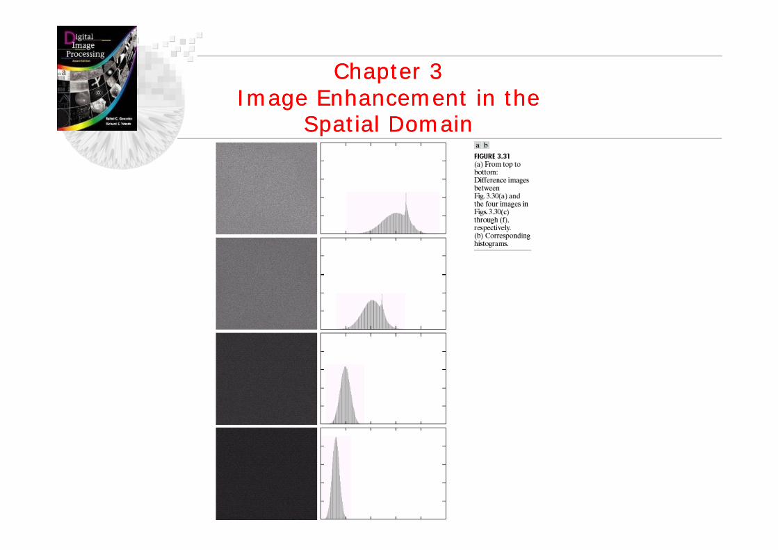
Chapter 3Chapter 3Image SubtractionImage Subtraction

Chapter 3Chapter 3Image SubtractionImage Subtraction

Chapter 3Chapter 3Image AveragingImage Averaging
Then
Chapter 3Chapter 3Image Enhancement in the
Spatial DomainImage Enhancement in the
Spatial Domain

Chapter 3Chapter 3
Sometime we need to manipulate values obtained from i hb i i l
Basics of Spatial FilteringBasics of Spatial Filtering
neighboring pixels
Example: How can we compute an average value of pixelsin a 3x3 region center at a pixel z?
4 1 2 262Pixel z
44 12
2 2643 4
29
676
92
725135
7
54 212735 8222
Image

Chapter 3Chapter 3Basic of Spatial FilterBasic of Spatial Filter

Chapter 3Chapter 3
S 1 S l d l d d i l
Basics of Spatial FilteringBasics of Spatial Filtering
Step 1. Selected only needed pixels
4 1 2 262Pixel z
…
4679
27243 49
74
6793 4
……
6254
5212
1357
6 13
…
35 8222

Chapter 3Chapter 3
S 2 M l i l i l b 1/9 d h h l
Basics of Spatial FilteringBasics of Spatial Filtering
…
Step 2. Multiply every pixel by 1/9 and then sum up the values
4679
3 4
…
676
913
……
…
4914
913
91
⋅+⋅+⋅=y
…
6917
919
91 ⋅+⋅+⋅+
X1
916
913
91 ⋅+⋅+⋅+1 1
1 1111 Mask or
Window or1
11
111
9 Window orTemplate

Chapter 3Chapter 3
Q ti H t t th 3 3 l t i l ?
Basics of Spatial FilteringBasics of Spatial Filtering
Question: How to compute the 3x3 average values at every pixels?
4 1 2 262Solution: Imagine that we havea 3x3 window that can be placed
h h i4679
27243 49
7
everywhere on the image
6254
5212
1357
Masking Window

Chapter 3Chapter 3
Step 1: Move the window to the first location where we want to
Basics of Spatial FilteringBasics of Spatial Filtering
compute the average value and then select only pixelsinside the window.
44 12
2 2643 4
29
Step 2: Computethe average value
3 3 1
4 12 3
29
676
92
725135
7 ∑∑= =
⋅=3
1
3
1
),(91
i j
jipy
Sub image p927
6254
5212
1357
Sub image p
Original imageStep 3: Place theresult at the pixel
4.3Original image result at the pixel
in the output imageStep 4: Move the
i d hOutput image
window to the next location and go to Step 2

Chapter 3Chapter 3
The 3x3 averaging method is one example of the mask
Basics of Spatial FilteringBasics of Spatial Filtering
operation or Spatial filtering.
The mask operation has the corresponding mask (sometimes p p g (called window or template).
The mask contains coefficients to be multiplied with pixelp pvalues.
Example : moving averagingw(2,1) w(3,1)
w(2,2) w(3,2)
w(1,1)
w(1,2)
1 11 1
111
w(3,3)w(3,2)w(3,1)
k ffi i
1119
Th k f h 3 3 iMask coefficients The mask of the 3x3 moving averagefilter has all coefficients = 1/9

Chapter 3Chapter 3
The mask operation at each point is performed by:1 Move the reference point (center) of mask to the
Basics of Spatial FilteringBasics of Spatial Filtering
1. Move the reference point (center) of mask to thelocation to be computed
2. Compute sum of products between mask coefficients and pixels in subimage under the mask.
… Mask frame
p(2,1)p(1,1) p(3,1)
…
w(2,1) w(3,1)w(1,1)
p(3,2)p(2,2)
p(2,3)
p(2,1)
p(3,3)p(1,3)
……
w(3,3)
w(2,2)
w(3,2)
w(3,2)w(1,2)
w(3,1)
…Subimage Mask coefficientsN M
∑∑= =
⋅=N
i
M
j
jipjiwy1 1
),(),(The reference pointof the mask
Chapter 3Chapter 3Basics of Spatial FilteringBasics of Spatial Filtering
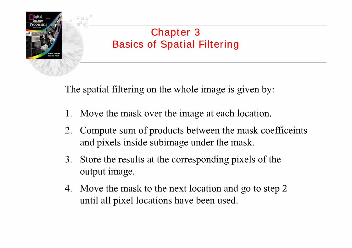
The spatial filtering on the whole image is given by:
1. Move the mask over the image at each location.
2. Compute sum of products between the mask coefficeintsand pixels inside subimage under the mask.
3. Store the results at the corresponding pixels of the output image.
4. Move the mask to the next location and go to step 2until all pixel locations have been used.

Chapter 3Chapter 3Chapter 3Basics of Spatial Filtering
Chapter 3Basics of Spatial Filtering
• Consider when the mask is moving near the edge of image.g g– Mask would not go out the image, so what is the
size of a result image?size of a result image?

Chapter 3Chapter 3Chapter 3Basics of Spatial Filtering
Chapter 3Basics of Spatial Filtering
• Consider when the mask is moving near the edge of image. How can we g g gkeep the size of original image? If the size of the mask is nxn.– Pad the image by adding (n-1)/2 rows or columns with 0’s– Pad with Replicating adding (n-1)/2 rows or columns.
• What are the effects?• How to do these with matlab or OpenCV?• How to do these with matlab or OpenCV?
0 0 0 00000
00
00
00
00
00
0 0 0 00000
00

Chapter 3Chapter 3Chapter 3Basics of Spatial Filtering
Chapter 3Basics of Spatial Filtering
• Is this Spatial Filter is linear operation?– What are Linear Spatial Filters?p
– What are Nonlinear Spatial Filters?

Chapter 3Chapter 3
Examples of the masks
Basics of Spatial FilteringBasics of Spatial Filtering
Examples of the masksSobel operators
0 11 2 111 11
3x3 moving average filter
0 1
100
2-1-21
-2 -1
102
0-101
1 1
111
1111
91
10-1 121P∂∂ compute to P
∂∂ compute to
111
x∂ y∂
3x3 sharpening filter (laplacian)-1 -18 -1
-1-11
-1-1-19

Chapter 3Chapter 3Chapter 3Basics of Spatial Filtering
Chapter 3Basics of Spatial Filtering
• Smoothing Spatial Filters– Smoothing Linear Filtersg
– Order-Statistics Filter (Nonlinear Filters)

Chapter 3Chapter 3Smoothing Linear FiltersSmoothing Linear Filters
• The first mask is a standard average of pixels under the mask sometimes called a box filter. An m x n mask would have a so e es ca ed a box filte . m x n as wou d ave anormalizing constant equal to 1/nm.
• The second mask called weighted average. Pixels are inversely weighted to as a function of their distance from the center of the mask.
• In practice it is difficult in general to see differences between• In practice, it is difficult in general to see differences between images smoothed by either of the masks.

Chapter 3Smoothing Linear Filter : Moving Average
Chapter 3Smoothing Linear Filter : Moving Average
Application : noise reductionand image smoothing
Di d t l h d t ilDisadvantage: lose sharp details
(Images from Rafael C. Gonzalez and Richard E. Wood, Digital Image Processing, 2nd Edition.g g g

Chapter 3Smoothing Linear Filter : Moving Average
Chapter 3Smoothing Linear Filter : Moving AverageSmoothing Linear Filter : Moving AverageSmoothing Linear Filter : Moving Average
(Images from Rafael C. Gonzalez and Richard E. Wood, Digital Image Processing, 2nd Edition.

Chapter 3O d St ti ti Filt
Chapter 3O d St ti ti FiltOrder-Statistic FiltersOrder-Statistic Filters
subimageOriginal image
Statistic parametersM M di M dMean, Median, Mode, Min, Max, Etc.
Moving window
Output imageNonlinear Filters

Chapter 3Chapter 3pOrder-Statistic Filters
pOrder-Statistic Filters
(Images from Rafael C. Gonzalez and Richard E. Wood, Digital Image Processing, 2nd Edition.

Chapter 3Chapter 3Chapter 3Order-Statistic Filters
Chapter 3Order-Statistic Filters
• Median Filters are particularly effective in presence of impulse noise, also called salt-p p ,pepper noise. Why?
• Salt-pepper noise appears as white and black dots superimposed on an image.

Chapter 3Chapter 3Chapter 3Sharpening Spatial Filters
Chapter 3Sharpening Spatial Filters
• Foundation– A basic definition of the first –order derivative of a one dimensional
function f(x) is the difference:function f(x) is the difference:–
( ) ( )xfxfxf
−+=∂∂ 1
An image function has two variables f(x,y), we use partial derivative in order to keep the notation the same.
x∂
– Similarly, we define a second-order derivative as the difference:
( ) ( ))1()()()1(2
xfxfxfxff−−−−+=
∂ ( ) ( )
)(2)1()1(
)1()()()1(
2
2
2
xfxfxff
xfxfxfxfx
−−++=∂
+∂
)(2)1()1(2 xfxfxfx
++∂

Chapter 3Sh i S ti l Filt
Chapter 3Sh i S ti l Filt
There are intensity discontinuities near object edges in an imageSharpening Spatial FiltersSharpening Spatial Filters
(Images from Rafael C. Gonzalez and Richard E. Wood, Digital Image Processing, 2nd Edition.

Chapter 3L l i Sh i H it k
Chapter 3L l i Sh i H it k
1Intensity profileEd
Laplacian Sharpening : How it worksLaplacian Sharpening : How it works
0
0.5f(x)Edge
20 40 60 80 100 120 140 160 180 2000.2
1st derivative
0 50 100 150 2000
0.1
dxdf
0 50 100 150 200
0
0.052nd derivative
0 50 100 150 200-0.05
0
2
2
dxfd
0 50 100 150 200

1 5
Chapter 3Laplacian Sharpening : How it works
Chapter 3Laplacian Sharpening : How it works
1
1.5
f(x)
0
0.5f(x)
0 50 100 150 200-0.5
1
1.5
2
)( fdf
0
0.5210)(dx
fdxf −
0 50 100 150 200-0.5
Laplacian sharpening results in larger intensity discontinuityLaplacian sharpening results in larger intensity discontinuity near the edge.

Chapter 3L l i Sh i H it k
Chapter 3L l i Sh i H it kLaplacian Sharpening : How it worksLaplacian Sharpening : How it works
B f h if(x)
Before sharpening
2 fdAfter sharpening
2
2
10)(dx
fdxf −

Chapter 3Chapter 3Chapter 3Summary First and Second order derivatives
Chapter 3Summary First and Second order derivatives
1. First-order derivatives generally produce thicker edges in an image.2. Second-order derivatives have a stronger response to fine detail, such as
thin lines and isolated pointsthin lines and isolated points.3. First-order derivatives generally have a stronger response to a gray-level
step.4. Second-order derivatives produce a double response at step changes in
gray level.
• The second derivative is better suited than the first derivative for image enhancement because of the ability of the former to enhance fine detail.
• The first derivative is for edge extraction, they do have important uses in conjunction with second derivative to obtain some impressive enhancement resultenhancement result

Chapter 3S d D i ti f E h t Th L l i
Chapter 3S d D i ti f E h t Th L l iSecond Derivatives for Enhancement The LaplacianSecond Derivatives for Enhancement The Laplacian

Chapter 3Laplacian Masks
Chapter 3Laplacian Masks
Used for estimating image Laplacian 2
2
2
22
yf
xff
∂∂
+∂∂
=∇Laplacian MasksLaplacian Masks
g g p
1 18 1
11
1 04 1
01
The center of the mask i i
1-81
1110
-41
110
is negative90o Isotropic Filters are 45o Isotropic
or-1 -1-1-1 00
Th f h k
Filters are rotation invariant
45 Isotropic Filters
-18-1
-1-1-10
4-1
-1-10
The center of the mask is positive
Application: Enhance edge, line, pointpp g pDisadvantage: Enhance noise

Chapter 3Laplacian Sharpening Example
Chapter 3Laplacian Sharpening Example
f f2∇
f2∇ ff 2∇f∇ ff 2∇−
(Images from Rafael C. Gonzalez and Richard E. Wood, Digital Image Processing, 2nd Edition.

Chapter 3Chapter 3Chapter 3Laplacian Sharpening
Chapter 3Laplacian Sharpening
• Laplacian is a derivative operation, its use highlights gray-level discontinuities in an image and deemphasizes regions with slowly varying gray levels This will trend to producewith slowly varying gray levels. This will trend to produce images that have grayish edge lines and other discontinuities, all superimpose on a dark, featureless background.p p , g
• To recover background features while still preserve the sharpening effect of Laplacian simply by adding the original and Laplacian images.

Chapter 3Chapter 3Chapter 3Laplacian Sharpening
Chapter 3Laplacian Sharpening
SimplificationWe implemented the Laplacian sharpening by first computing the L l i filt d i d th bt ti it f th i i lLaplacian-filtered image and then subtracting it from the original image. We can computer a one pass mask:
Mask forMask forf2∇ ff 2∇−
1 18 1
11
-1 -19 1
-11
-1 05 1
01
1 0-4 1
01 oror
1-81
111 -1
9-1
-1-1-10
5-1
-1-100
-41
110
o

Chapter 3Laplacian Sharpening Example
Chapter 3Laplacian Sharpening Example
ff 2∇−Mask for
-1 -19 1
-11
-1 05 1
01 or
-19-1
-1-1-10
5-1
-1-10
orMask for
f2∇
1 11
f∇
1-81
111
or1 0-4 1
01
or
041
110
(Images from Rafael C. Gonzalez and Richard E. Wood, Digital Image Processing, 2nd Edition.

Chapter 3Chapter 3Chapter 3Unsharp Masking and High-Boost Filtering
Chapter 3Unsharp Masking and High-Boost Filtering
• A process to sharpen images (in the publishing industry) consists of subtracting a blurred version of image from the image itself called unsharp masking expressed as:image itself, called unsharp masking, expressed as:
• A slight further generalization of unsharp masking is called• A slight further generalization of unsharp masking is called high-boost filtering. fhb is defined at any point (x,y) as:
• As before is a blurred version of f, so fhb can rewrite as:f
• Then

Chapter 3Chapter 3Unsharp Masking and High-Boost FilteringUnsharp Masking and High-Boost Filtering
-1 -1-1 -1 00
1
A+8
1
-1-1
1 0
A+4
1
-1-1
0-1-1-1 0-10
Equation:Equation:
⎨⎧ ∇−
=),(),(
),(2
2 yxfyxAfyxfhb
The center of the mask is negative
⎩⎨
∇+ ),(),(),(
2 yxfyxAfyfhb The center of the mask is positive

Chapter 3Unsharp Masking and High-Boost Filtering
Chapter 3Unsharp Masking and High-Boost Filtering
(Images from Rafael C. Gonzalez and Richard E. Wood, Digital Image Processing, 2nd Edition.

Chapter 3First Order Derivative
Chapter 3First Order Derivative
0.5
1
f(x) Edges
First Order DerivativeFirst Order Derivative
20 40 60 80 100 120 140 160 180 2000
Intensity profile( ) g
0
0.21st derivativedf
0 50 100 150 200-0.2
1st deri ati e
dx
0.1
0.21st derivative
df
0 50 100 150 2000
dx

Chapter 3First Order Derivative
Chapter 3First Order Derivative
Sobel operators
First Order DerivativeFirst Order Derivative
M h i ll h di f i bl f i (h h iMathematically, the gradient of a two-variable function (here the image intensity function) is at each image point a 2D vector with the components given by the derivatives in the horizontal and vertical directions. At each image point, the gradient vector points in the direction of largest possible intensity increase, and the length of the gradient vector corresponds to the rate of change in that direction. g

Chapter 3First Order Derivative
Chapter 3First Order Derivative
0 1-1 -2 -1-1f∂ f∂tt
First Order DerivativeFirst Order Derivative
Sobel operators1
0
0
2-2
-1 1
0
2
00
1xf∂∂computeto y
f∂
computeto
Sobel operators
fxf∂∂
yf∂∂

Chapter 3First Order Partial Derivative: Image Gradient
Chapter 3First Order Partial Derivative: Image Gradient
f∂f x
f∂∂
f∂ f∇
y∂

imfilterimfilter imfilter O ti D i tiimfilter Multidimensional image filtering Syntax:B = imfilter(A,H)B = imfilter(A H option1 option2 )
Option Description
X Input array values outside the bounds of the array are implicitly assumed toB = imfilter(A,H,option1,option2,...)
DescriptionB = imfilter(A,H) filters the multidimensional array A
with the multidimensional filter H. The array A can be a nonsparse numeric array of any class
the array are implicitly assumed to have the value X. When no boundary option is specified, imfilter uses X = 0.
' t i I t l t id th b d fp y y
and dimension. The result B has the same size and class as A.
Each element of the output B is computed using double precision floating point If A is an integer
'symmetric'
Input array values outside the bounds of the array are computed by mirror-reflecting the array across the array border.
double-precision floating point. If A is an integer array, then output elements that exceed the range of the integer type are truncated, and fractional values are rounded.
'replicate' Input array values outside the bounds of the array are assumed to equal the nearest array border value.
B = imfilter(A,H,option1,option2,...) performs multidimensional filtering according to the specified options. Option arguments can have the following values.
Boundary Options
'circular' Input array values outside the bounds of the array are computed by implicitly assuming the input array is periodic
ou da y Op o s

fspecialp
f i l V l D i ifspecial Create special 2-D filtersSyntax
Value Description
'average' Averaging filter
h = fspecial(type)h = fspecial(type,parameters)Description
'disk' Circular averaging filter (pillbox)
'gaussian' Gaussian lowpass filter
h = fspecial(type) creates a two-dimensional filter h of the specified type. fspecial returns h as a correlation kernel hich is
'laplacian' Approximates the two-dimensional Laplacian operator
'log' Laplacian of Gaussian filteras a correlation kernel, which is the appropriate form to use with imfilter. type is a string having one of these values.
'motion' Approximates the linear motion of a camera
' itt' P itt h i t l d'prewitt' Prewitt horizontal edge-emphasizing filter
'sobel' Sobel horizontal edge-emphasizing filterfilter
'unsharp' Unsharp contrast enhancement filter
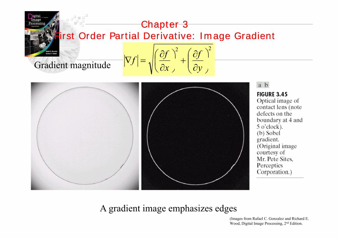
Chapter 3First Order Partial Derivative: Image Gradient
Chapter 3First Order Partial Derivative: Image Gradient
22
⎟⎟⎠
⎞⎜⎜⎝
⎛∂∂
+⎟⎠⎞
⎜⎝⎛∂∂
=∇fffGradient magnitude
First Order Partial Derivative: Image GradientFirst Order Partial Derivative: Image Gradient
⎟⎠
⎜⎝ ∂⎠⎝ ∂ yx
fGradient magnitude
A gradient image emphasizes edges(Images from Rafael C. Gonzalez and Richard E. Wood, Digital Image Processing, 2nd Edition.

Chapter 3First Order Partial Derivative: Image Gradient
Chapter 3First Order Partial Derivative: Image GradientFirst Order Partial Derivative: Image GradientFirst Order Partial Derivative: Image Gradient
xf∂∂
yf∂∂
I=imread('fig345.jpg');I=double(I);( )h1=fspecial('sobel');h2=h1';I1=imfilter(I,h1);figure; imshow(I1);g ( )I2=imfilter(I,h2);figure; imshow(I2);I3=sqrt(imfilter(I,h1).^2+imfilter(I,h2).^2);figure; imshow(uint8(I3));
(Images from Rafael C. Gonzalez and Richard E. Wood, Digital Image Processing, 2nd Edition.

Image Enhancement in the Spatial Domain : Image Enhancement in the Spatial Domain : Mix things up !
f2∇ f∇
f∇DA smoothB D
+ -+
Sharpening EC (Images from Rafael C. Gonzalez and Richard E. Wood, Digital Image Processing, 2nd Edition.

Image Enhancement in the Spatial Domain : Image Enhancement in the Spatial Domain : Mix things up !
G PowerL TEC
G Law Tr.
Σ
F
Σ
MultiplicationF A
H(Images from Rafael C. Gonzalez and Richard E. Wood, Digital Image Processing, 2nd Edition.

Filtering Using imfilter in MatlabFiltering Using imfilter in MatlabFiltering Using imfilter in MatlabFiltering Using imfilter in Matlab
Filtering of images either by correlation or convolution can be performed using theFiltering of images, either by correlation or convolution, can be performed using the toolbox function imfilter. This example filters an image with a 5-by-5 filter containing equal weights. Such a filter is often called an averaging filter.
I = imread('coins png');I = imread( coins.png );h = ones(5,5) / 25;I2 = imfilter(I,h);imshow(I), title('Original Image');figure, imshow(I2), title('Filtered Image')

Filtering Using imfilter in MatlabFiltering Using imfilter in MatlabFiltering Using imfilter in MatlabFiltering Using imfilter in Matlab
B = imfilter(A H option1 option2 )B = imfilter(A, H, option1, option2,...)

Imfilter pad with 0Imfilter pad with 0Imfilter pad with 0Imfilter pad with 0
I = imread('eight.tif');h = ones(5,5) / 25;I2 = imfilter(I,h);imshow(I), title('Original Image');figure, imshow(I2), title('Filtered Image with Black Border')
Effect of zeros padding

Imfilter pad with replicationImfilter pad with replicationImfilter pad with replicationImfilter pad with replication
I = imread('eight tif');I = imread( eight.tif );h = ones(5,5) / 25;I3 = imfilter(I h 'replicate');I3 = imfilter(I,h, replicate );figure, imshow(I3); title('Filtered Image with Border Replication')title('Filtered Image with Border Replication')
No Effect

Imfilter paddingImfilter paddingImfilter paddingImfilter padding
• What are results from 'circular' and 'symmetric‘ options?y p

Create predefined 2-D filterCreate predefined 2-D filterpp
h = fspecial(type)h = fspecial(type parameters)h = fspecial(type, parameters)
>> h = fspecial('sobel')h =
1 2 11 2 10 0 0
-1 -2 -1>> h'>> hans =
1 0 -12 0 22 0 -21 0 -1
>> h=fspecial('disk',5)>> h=fspecial('laplacian',)

Filtering Using imfilterFiltering Using imfilter
• Correlation and Convolution Options
Option Description'corr' imfilter performs multidimensional filtering usingcorr imfilter performs multidimensional filtering using
correlation, which is the same way that filter2 performs filtering. When no correlation or convolution option is specified, imfilter uses correlation.
'conv' imfilter performs multidimensional filtering using convolution.

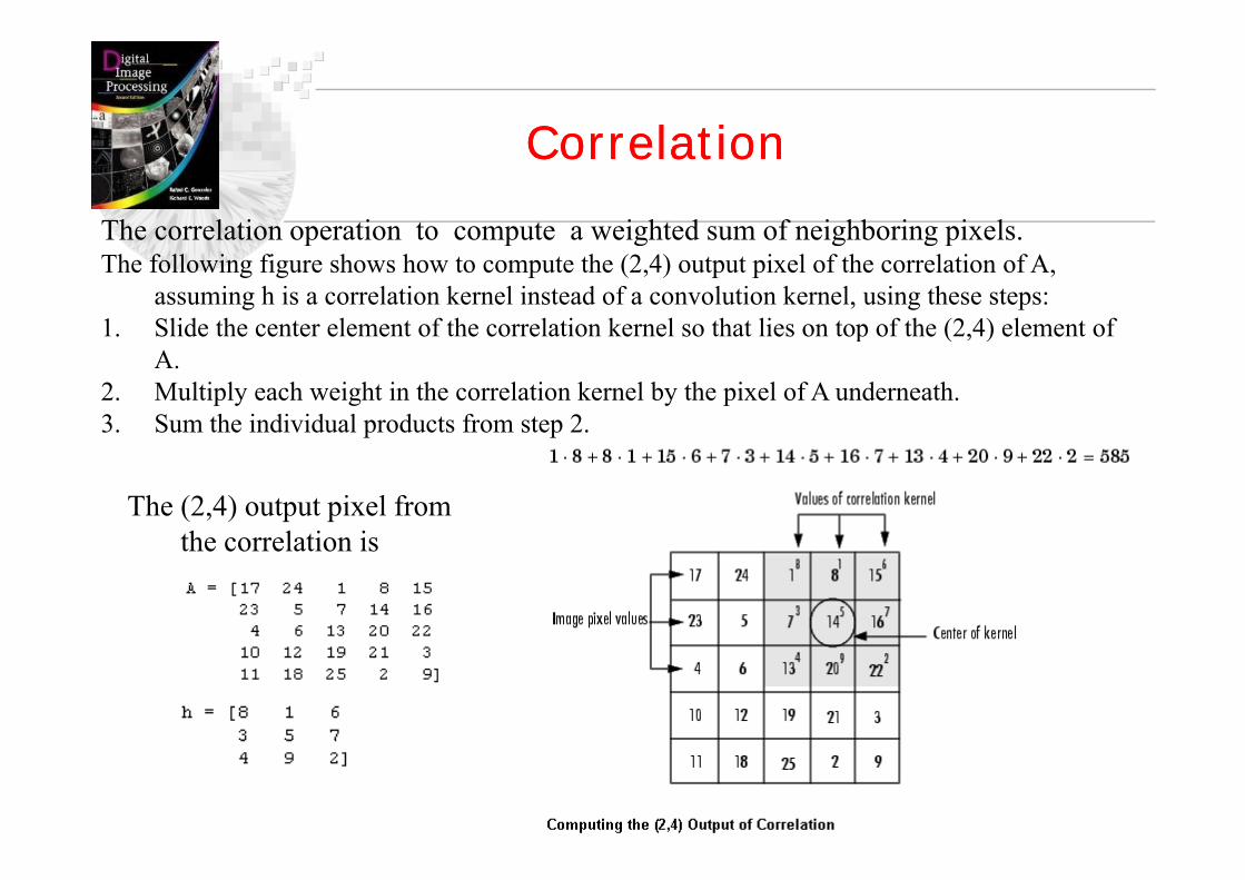
CorrelationCorrelationCorrelationCorrelation
The correlation operation to compute a weighted sum of neighboring pixels.p p g g g pThe following figure shows how to compute the (2,4) output pixel of the correlation of A,
assuming h is a correlation kernel instead of a convolution kernel, using these steps: 1. Slide the center element of the correlation kernel so that lies on top of the (2,4) element of p ( , )
A. 2. Multiply each weight in the correlation kernel by the pixel of A underneath. 3. Sum the individual products from step 2.
The (2,4) output pixel from the correlation isthe correlation is

L ti I F tL ti I F tLocating Image FeaturesLocating Image Features
C l i b d l f i hi i i hiCorrelation can be used to locate features within an image; in this context correlation is often called template matching.
bw =double( imread('text.png'));a = bw(32:45,88:98); ( , );C = imfilter(bw,a);figure, imshow(C,[]);
(C( ))max(C(:))ans = 68.0000thresh = 60;thresh 60;figure, imshow(C > thresh)

ConvolutionConvolutionConvolutionConvolution
Convolution is a neighborhood operation in which each output pixel is the weighted sum ofConvolution is a neighborhood operation in which each output pixel is the weighted sum of neighboring input pixels. The matrix of weights is called the convolution kernel, also known as the filter. A convolution kernel is a correlation kernel that has been rotated 180 degrees
The following figure shows how to compute the (2,4) output pixel using these steps: h l i k l d b i l1. Rotate the convolution kernel 180 degrees about its center element.
2. Slide the center element of the convolution kernel so that it lies on top of the (2,4) element of A.
3 Multiply each weight in the rotated convolution kernel by the pixel of A underneath3. Multiply each weight in the rotated convolution kernel by the pixel of A underneath. 4. Sum the individual products from step 3.


Statistics Filter (nonlinear filter)Statistics Filter (nonlinear filter)Statistics Filter (nonlinear filter)Statistics Filter (nonlinear filter)
B = ordfilt2(A, order, domain)domain is equivalent to the structuring element used for binary i ti It i t i t i i l 1' d 0' th 1'image operations. It is a matrix containing only 1's and 0's; the 1's define the neighborhood for the filtering operation.
For example, B dfilt2(A 5 (3 3)) i l t 3 b 3 di filtB = ordfilt2(A,5,ones(3,3)) implements a 3-by-3 median filter; B = ordfilt2(A,1,ones(3,3)) implements a 3-by-3 minimum filter; B dfilt2(A 9 (3 3)) i l t 3 b 3 i filtB = ordfilt2(A,9,ones(3,3)) implements a 3-by-3 maximum filter. B = ordfilt2(A,1,[0 1 0; 1 0 1; 0 1 0]) replaces each element in A
by the minimum of its north east south and west neighborsby the minimum of its north, east, south, and west neighbors.

Statistics Filter (nonlinear filter)Statistics Filter (nonlinear filter)Statistics Filter (nonlinear filter)Statistics Filter (nonlinear filter)
B = medfilt2(A, [m n]) performs median filtering of the matrix A in two dimensions.
E h t t i l t i th di l i th bEach output pixel contains the median value in the m-by-n neighborhood around the corresponding pixel in the input image medfilt2 pads the image with 0's on the edges so theimage. medfilt2 pads the image with 0 s on the edges, so the median values for the points within [m n]/2 of the edges might appear distorted.
B = medfilt2(A) f ( )performs median filtering of the matrix A using the default 3-by-
3 neighborhood.

Median FilterMedian FilterMedian FilterMedian Filter
I = imread('eight.tif');figure, imshow(I);J = imnoise(I 'salt & pepper' 0 02);J imnoise(I, salt & pepper ,0.02);K = medfilt2(J);figure, imshow(J), figure, imshow(K)