Embed Size (px)
Citation preview
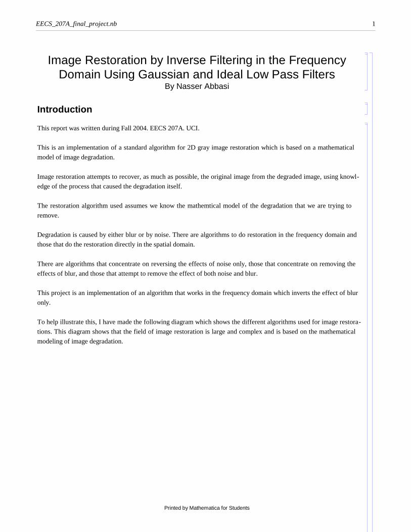
Image Restoration by Inverse Filtering in the Frequency Domain Using Gaussian and Ideal Low Pass Filters
By Nasser Abbasi
Introduction
This report was written during Fall 2004. EECS 207A. UCI.
This is an implementation of a standard algorithm for 2D gray image restoration which is based on a mathematical
model of image degradation.
Image restoration attempts to recover, as much as possible, the original image from the degraded image, using knowl-
edge of the process that caused the degradation itself.
The restoration algorithm used assumes we know the mathemtical model of the degradation that we are trying to
remove.
Degradation is caused by either blur or by noise. There are algorithms to do restoration in the frequency domain and
those that do the restoration directly in the spatial domain.
There are algorithms that concentrate on reversing the effects of noise only, those that concentrate on removing the
effects of blur, and those that attempt to remove the effect of both noise and blur.
This project is an implementation of an algorithm that works in the frequency domain which inverts the effect of blur
only.
To help illustrate this, I have made the following diagram which shows the different algorithms used for image restora-
tions. This diagram shows that the field of image restoration is large and complex and is based on the mathematical
modeling of image degradation.
EECS_207A_final_project.nb 1
Printed by Mathematica for Students
Types of image degradation
blurring noise
Lens blurCamera PSF (pointspread function)
Motionblur
Due to electronics of camera Due to quantization(digital camera,CCD,…)
Noise models (Probability density functions)
Gaussian Gamma Uniform Periodic (dueto electronicsin camera)
Impulse(salt/pepper)
Rayleigh
Exponential
Median(nonlinear)
Restoration of noise only algorithms
Spatial based methods (filtering)(use when additive noise is present)
Frequency based methods
Mean filters
Arithmeticmean
Geometricmean
Harmonicmean
Contraharmonicmean
Statistics based filters
Max/Min
MidpointAlpha-
mean
Adaptivefilters
Periodicnoisereduction
Band-reject Band-pass Notch filters
Methods ofestimationof PSF
By Imageobservation
Byexperimentation
By Mathematicalmodeling
Algorithms that incorporates degradation due to PSF and noise
Minimum mean square error (Wiener) filtering(requires knowledge of the original undegradedimage power spectra and of the power spectra ofthe noise
Constrained least square filtering
Requires knowledge onlyof the mean andvariance of the noise
Geometric mean filter
(Generalized form of Wiener filtering) alsocalled the spectrum equalization filter.
Geometric transformation algorithms for restoration
These class of algorithms modify the spatial relati onships between pixels in theimage. Also called Rubber-sheet transformations.
This projectimplementsthis algorithmfor theGaussian andIdeal low passfilters
Overview.vsdby Nasser AbbasiDecember 6, 2004
IdealLowPass
Gaussianlow pass
Butterworthlow pass
Direct inversefiltering (infrequencydomain)
Atmosphericturbulencemodel
Linearmotionblurmodel
As can be seen from the diagram above, it is important to know that different blur degradations require the use of
EECS_207A_final_project.nb 2
Printed by Mathematica for Students

different PSF (Point Spread Function) mathematical model.
For example, motion blur would require different PSF than say a degradation caused by ripple distortion or by a
normal blur degradation. Even blur degradation itself has many different types (motion, lens, Gaussian, Radial, etc...)
and different mathematical function for PSF would be needed for each type to obtain an accurate restoration that
matches the original image as best as possible. For instance, degradation by motion blur, would require a mathematical
function for PSF which would take an estimate of the linear or radial motion parameters that caused the blur.
Given the above, and to be able to illustrate the direct inversion algorithm, I had to assume a certain PSF model. I have
selected to use the 2D Gaussian low pass filter and the 2D ideal low pass filter. Using these filters, I will start by
generating a number of degraded images from an original single undegraded image. I will use different standard
deviation values for the Gaussian for each generation of a degraded image, and different radius values for the ideal low
pass filter.
In this case, the standard deviation used for the Gaussian is nothing but the radius as well. The radius is measured as
the number of pixels from the center or the spectrum. In all cases, the 2D spectrum will be centered in the middle of
the image.
After degrading the original image, I will then restore these images using the inverse filtering algorithm and compare
the result with the original, undestorted image. I will observer how using different radius values affect the restoration
quality, and will compare visually each restored image to the original image and comment on the quality of the restora-
tion.
The standard image of Lena will be used throughout this evaluation. It is a gray level, 512 x 512 pixels image that I
downloaded from the internet. I have used a gray level image to simplify the implementation, otherwise I would have
to perform 2D fourier transformation and inverse transformation on each of the 3 channels. For the purpose of illustrat-
ing the algorithm, I did not feel this would not have adding any more value.
The restoration algorithm can be implemented completely in the spatial domain if needed. However, since the algo-
rithm requires performing a convolution operation, and since convolution in the spatial domain is equivalent to multipli-
cation in the frequency domain, we will start by transforming the input image to the frequency domain to take advan-
tage of the speed of the FFT (Fast Fourier Transforms).
In this implementation, an image is read, degraded using the PSF, and then restored using the direct inversion algo-
rithm. Both the degraded and restored images are saved to disk.
The name of the output image file will be the same as the input image file, but with the word _RESTORED and
_DEGRADED appended to the file name. The type of the images outputted will be in the same graphic format as the
input image.
This diagram below illustrates the data flow of the program as a black box
EECS_207A_final_project.nb 3
Printed by Mathematica for Students

Degraded image“test_DEGRADED.gif”
restored image“test_RESTORED.gif”
Restorationalgorithm
Original image ‘f’“test.gif”
LOOP
Apply differentGaussian standarddeviation degradation(PSF) to image
END LOOP
A small note on how this report was written
This report was itself written in Mathematica in the same file as the program itself. This made it easier to add com-
ments on the program and have these as part of the report itself as the same time. This feature is attractive since it
eliminates the need to separate the program from the documentation or the report as would be the case in other
systems.
Project Details
Mathematical model of image degradation
The algorithm is based on the following mathematical model of image degradation.
Let the degraded image be called g. Let the camera PSF (point spread function) be called h (This is the degradation
function which depends on the system itself, i.e. the camera). Let noise introduced into the degraded image be called h.
Let the original, undegraded image be called f .
The degraded image is now given by
gHx, yL = hHx, yL≈ f Hx, yL + hHx, yLWhere the operator ≈ is the convolution operator.
Taking the 2D fourier transform results in
GHu, vL = HHu, vL FHu, vL + NHu, vLIn this implementation we assume that noise is zero. This results in the following relation
GHu, vL = HHu, vL FHu, vLHence,
FHu, vL = GHu,vLÅÅÅÅÅÅÅÅÅÅÅÅÅÅÅÅHHu,vL
Now, to obtain the restored image, we perform a 2D inverse fourier transform, let the restored image be f̀
EECS_207A_final_project.nb 4
Printed by Mathematica for Students
f̀ = Inverse_2D_Fourier_Transform ( F(u,v) )
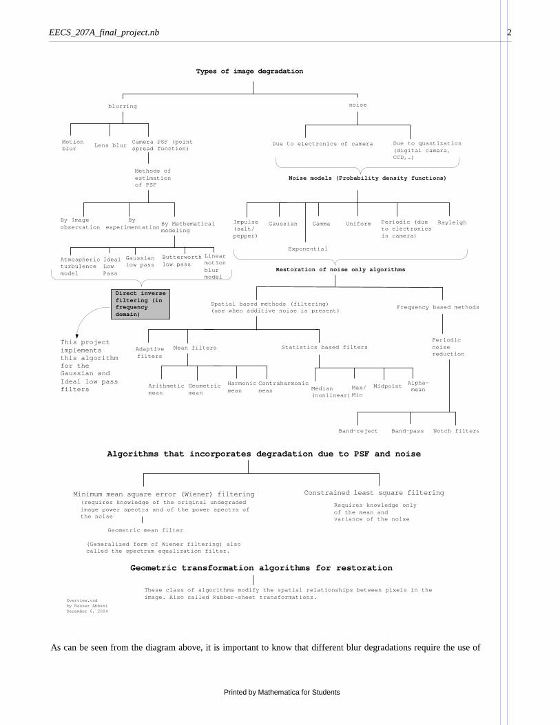
Notice that f̀ Hx, y) (the restored image) will not be exactly the same as f Hx, yL for the following reasons
1. We do not know exactly what the camera PSF function is, we will assume here that the PSF is a 2D Gaussian
filter with a certain standard deviation or an ideal low pass filter.
2. We did not model the noise in this implementation. Noise is difficult to model and depends on many factors.
The following diagram illustrates this process
fOriginal, noisefree, degradationfree, object.
Camera systemPSF assumed h
g degraded
image
noise
Restorationalgorithm
f' restored
image
PSF model
This is the most important function to select for the restoration, since this is how we assume the degradation has
occurred in the first place. The following 2D gaussian filter is assumed for the PSF (this is the PSF expressed in the
frequency domain)
HHu, vL = ‰- D2 Hu,vLÅÅÅÅÅÅÅÅÅÅÅÅÅÅÅÅÅ2s2
For the low pass filter, we use this definition
HHu, vL = 1 If DHu, vL ¥ D0 else 0 where D0 is the distance from the center of the spec-
trum to the point (u,v)
Algorithm steps
The following are the detailed step by step of the algorithm
1. Ask the user for the image file name
2. Read the image to memory to a matrix f Hx, yL3. Generate N numbers of HHu, vL (PSF) filters (using different Gaussian standard deviations, or different radius
values with a fixed increments). For example, use 3,5,10,20,40 pixels. This results in N PSF matrices H(u,v) call themHiHu, vL, ..., HnHu, vL4. Do step 3 for both the Gaussian and the Ideal low pass filters.
5. Multiply the input image f(x,y) by H-1Lx+y
6. Obtain the 2D fourier transform of the original image, call it FHu, vL. Due to step 5, this spectrum is now centered.
7. For each PSF H(u,v), generate 2D Fourier transform of a degraded image using GiHu, vL = HiHu, vL *FHu, vL
EECS_207A_final_project.nb 5
Printed by Mathematica for Students

8. For each GiHu, vL generate the spatial image giHx, vL by taking the 2D inverse fourier transform.
9. Take the real part of the image generated in step 8.
10. Multiply the result of step 9 by H-1Lx+y to get a centered image.
11. Save each of the degraded images giHx, vL to allow more analysis if needed by external programs such as photoshop.
12. Start the restoration pass. For each GiHu, vL obtain the restored fourier transform Fi` Hu, vL = GiHu,vLÅÅÅÅÅÅÅÅÅÅÅÅÅÅÅÅÅHiHu,vL
13. For each Fi` Hu, vL apply the 2D IDFT to obtain the restored image f̀ iHx, yL
14. Save these images to disk for analysis.
15. Examine visually each of the images f̀ iHx, yL and comment of the quality of restoration by comparing them to the
original image f(x,y).
Implementation issues
The main issue to handle in the implementation of the algorithm is the step when we divide FHu, vL = GHu,vLÅÅÅÅÅÅÅÅÅÅÅÅÅÅÅÅHHu,vL . This is
because H can be zero if we use a large standard deviation for the Gaussian. This problem was resolved by explicitly
checking for a zero value in the denominator. When this is detected, we set the corresponding value in F(u,v) to 0. This
has the effect of setting those high frequencies to zero. Since it is noise that usually occupies the high frequency parts
of the image spectrum , this should not cause siginfication problems in the restoration.
Output, Tables and Results
Conclusions
For small radius values, using the Gaussian low pass filter resulted in an acceptable restoration. The ideal low pass
filter however produced no restoration that can be detected.
This can be explained by the fact that an ideal low pass filter is not a causual filter and do not occur naturally.
We notice that for a small radius, more image power will be lost in the degradation process, since image power is
mostly concentrated in small circles around the center of the 2D spectrum. As the radius is increased, the effect of the
restoration decreased until at about radius 100 pixels, there was no restoration that can be noticed.
This project shows that the choice of restoration PSF is critical. It is not possible to use a generic PSF function to
restore different degraded images with without having some knowledge of the cause of the degradation to be able to
model a PSF which will best restore the image.
If one is able to estimate the PSF, and can ignore the noise, then this algorithm becomes attractive due to its speed
when performed in the frequency domain by utilizing the Fast Fourier Transform and due to its simplicity.
Future work and possible extensions to this project
The following are possible options that this work can be expanded on.
1. Investigate other PSF models such as the Butterworth filter.
2. Investigate how to do restoration with the presence of noise by the use of such filters as minimum mean square error
(Wiener) or the constrained least square filtering method. These methods are more mathematically complicated, but
EECS_207A_final_project.nb 6
Printed by Mathematica for Students
are considered to produce better resortation results.
3. Investigate the restoration of motion blur.
Sample run and output
Here, I show a complete typical run output of this program. This output will use both the Gaussian and Ideal low pass
filters.
Start by initialization of the workspace and loading the needed packages
Remove@"Global` ∗" D;<< nma.m<< ImageProcessing`<< Graphics`Graphics3D`<< Geometry`Rotations`
define the PSF functionH∗ this is actually distance square ∗Ld@u_, v_, nRow_, nCol_ D : = RoundANAJu − J nRow�������������
2NN2 + Jv − J nCol�������������
2NN2EEH∗This is the Gaussian low pass filter ∗L
g2D@u_, v_, σ_D : = �− distanceMatrix @@u,v DD��������������������������������������������������������2 σ2H∗THis is an ideal low pass filter ∗L
gIdealLowPass @D0_, u_, v_, nRow_, nCol_ D : = Module @8response <,
If @Round@N@Sqrt @d@u, v, nRow, nCol DDDD ≤ D0, response = 1, response = 0D;
responseDDisplay PSF using standard deviation of 6 and 40 pixels just for illustration purposes. We will use s=6 here.
EECS_207A_final_project.nb 7
Printed by Mathematica for Students
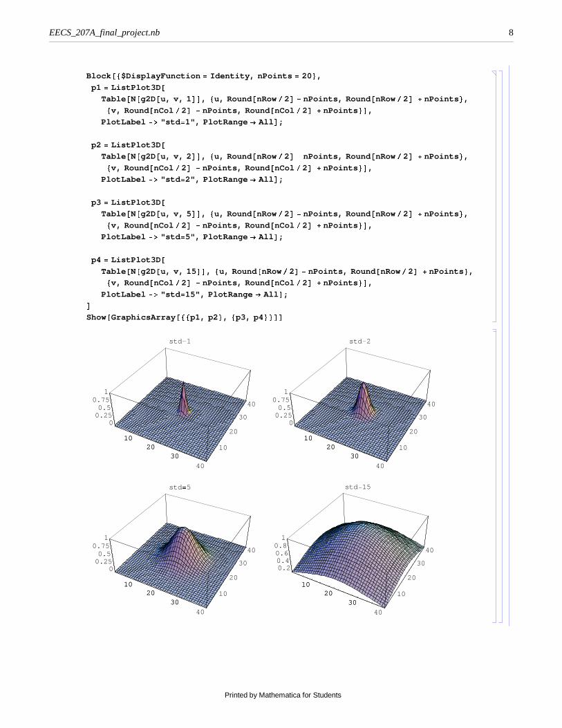
Block @8$DisplayFunction = Identity, nPoints = 20<,
p1 = ListPlot3D @Table @N@g2D@u, v, 1 DD, 8u, Round @nRowê 2D − nPoints, Round @nRowê 2D + nPoints <,8v, Round @nCol ê2D − nPoints, Round @nCol ê 2D + nPoints <D,
PlotLabel −> "std =1", PlotRange → All D;
p2 = ListPlot3D @Table @N@g2D@u, v, 2 DD, 8u, Round @nRowê 2D − nPoints, Round @nRowê 2D + nPoints <,8v, Round @nCol ê2D − nPoints, Round @nCol ê 2D + nPoints <D,
PlotLabel −> "std =2", PlotRange → All D;
p3 = ListPlot3D @Table @N@g2D@u, v, 5 DD, 8u, Round @nRowê 2D − nPoints, Round @nRowê 2D + nPoints <,8v, Round @nCol ê2D − nPoints, Round @nCol ê 2D + nPoints <D,
PlotLabel −> "std =5", PlotRange → All D;
p4 = ListPlot3D @Table @N@g2D@u, v, 15 DD, 8u, Round @nRowê 2D − nPoints, Round @nRowê 2D + nPoints <,8v, Round @nCol ê2D − nPoints, Round @nCol ê 2D + nPoints <D,
PlotLabel −> "std =15", PlotRange → All D;DShow@GraphicsArray @88p1, p2 <, 8p3, p4 <<DD
std =5
1020
30
40
10
20
30
40
00.250.5
0.751
1020
30
std =15
1020
30
40
10
20
30
40
0.20.40.60.8
1
1020
30
std =1
1020
30
40
10
20
30
40
00.250.5
0.751
1020
30
std =2
1020
30
40
10
20
30
40
00.250.5
0.751
1020
30
EECS_207A_final_project.nb 8
Printed by Mathematica for Students
Now, set the working directory to be the same working directory as this note book to allow easy input of
file names for the degraded images.
nma`cd
Directory @DNow ask the user for the image file name, and read it to memoryH∗fileName =Input @"Please enter the degraded image file name" D; ∗Lsample a 2D continuos gaussian to obtain a discrete version of Gaussian 2D,to use as a filtering window to convolve
the image with
fileName = "triangle.jpg";
fileName = "lena_gray_blur_gaussian_6";
fileName = "test";
fileName = "lena_gray";
format = "JPG";
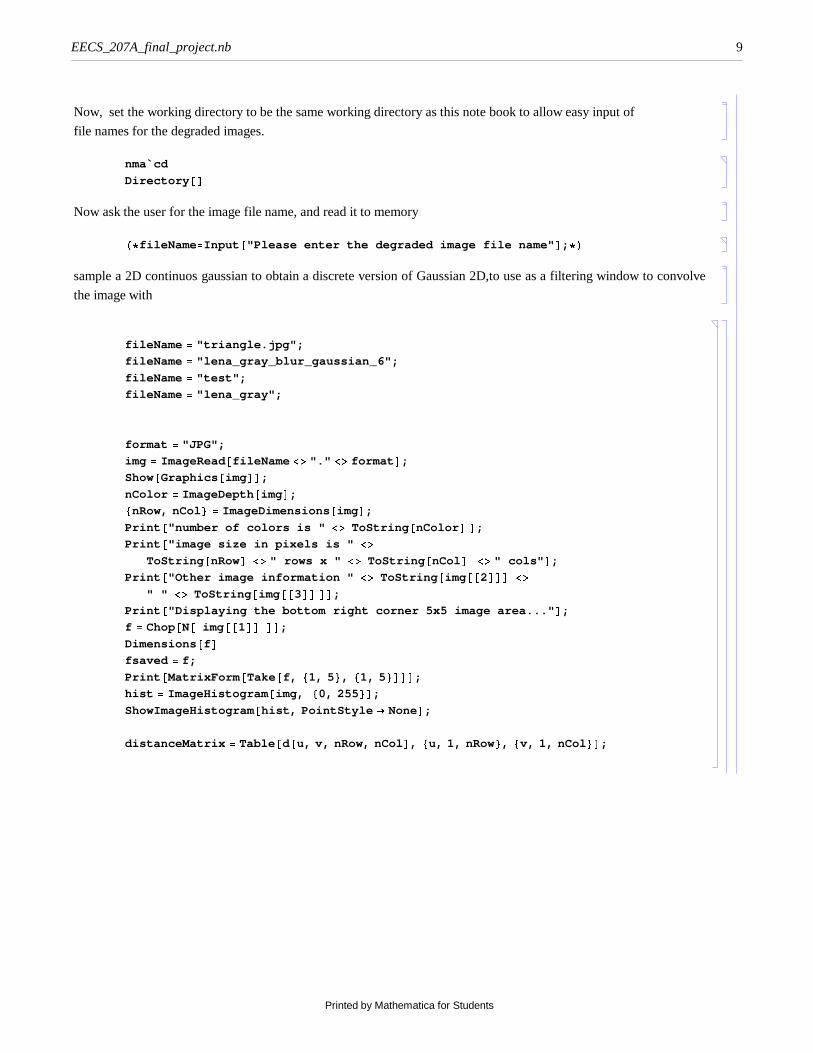
img = ImageRead @fileName <> "." <> format D;
Show@Graphics @img DD;
nColor = ImageDepth @img D;8nRow, nCol < = ImageDimensions @img D;
Print @"number of colors is " <> ToString @nColor D D;
Print @"image size in pixels is " <>ToString @nRowD <> " rows x " <> ToString @nCol D <> " cols" D;
Print @"Other image information " <> ToString @img @@2DDD <>" " <> ToString @img @@3DD DD;
Print @"Displaying the bottom right corner 5x5 image area..." D;
f = Chop@N@ img @@1DD DD;
Dimensions @f Dfsaved = f;
Print @MatrixForm @Take@f, 81, 5 <, 81, 5 <DDD;
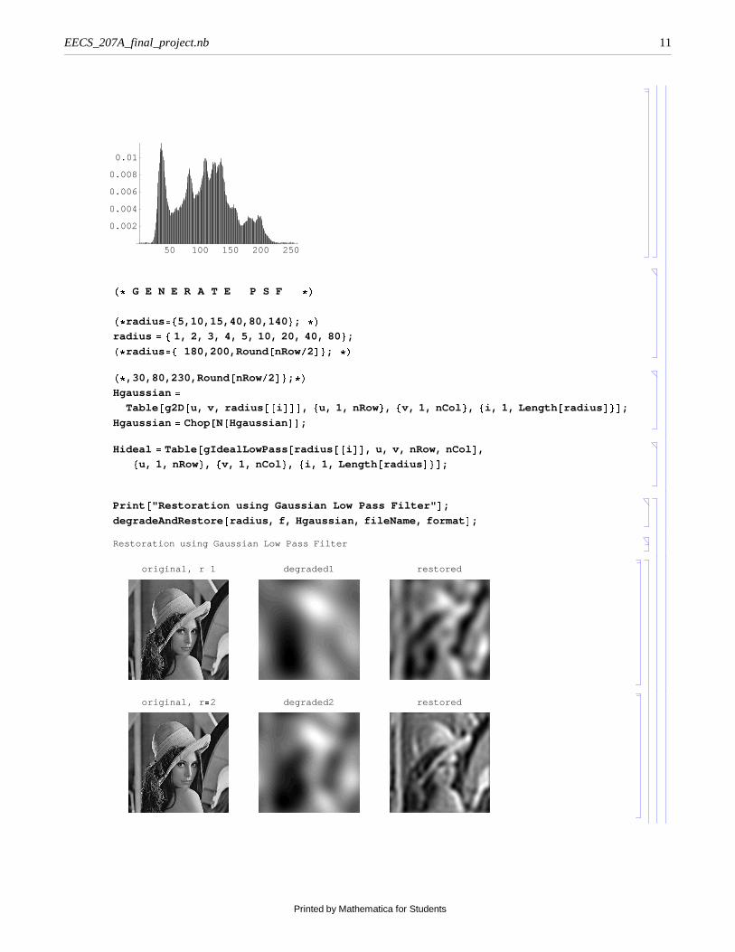
hist = ImageHistogram @img, 80, 255 <D;
ShowImageHistogram @hist, PointStyle → NoneD;
distanceMatrix = Table @d@u, v, nRow, nCol D, 8u, 1, nRow <, 8v, 1, nCol <D;
EECS_207A_final_project.nb 9
Printed by Mathematica for Students
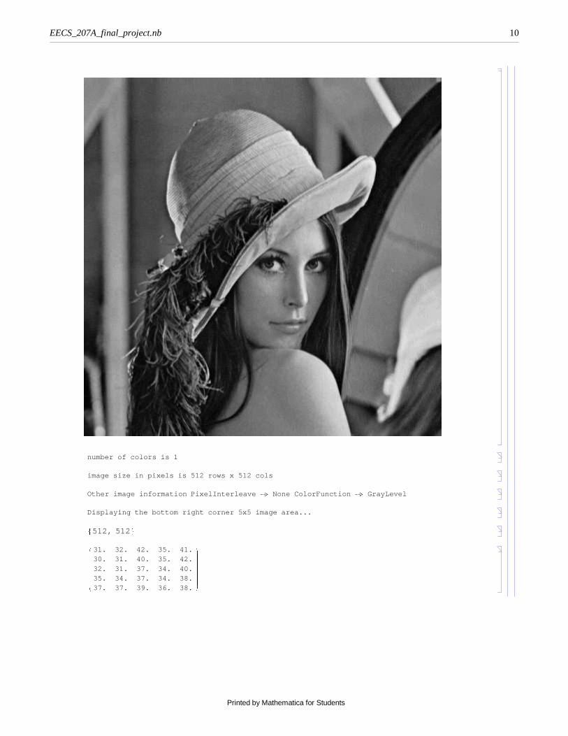
number of colors is 1
image size in pixels is 512 rows x 512 cols
Other image information PixelInterleave −> None ColorFunction −> GrayLevel
Displaying the bottom right corner 5x5 image area...8512, 512 <ikjjjjjjjjjjjjjjjj 31. 32. 42. 35. 41.30. 31. 40. 35. 42.32. 31. 37. 34. 40.35. 34. 37. 34. 38.37. 37. 39. 36. 38.
y{zzzzzzzzzzzzzzzz
EECS_207A_final_project.nb 10
Printed by Mathematica for Students
50 100 150 200 250
0.002
0.004
0.006
0.008
0.01
H∗ G E N E R A T E P S F ∗LH∗radius =85,10,15,40,80,140 <; ∗Lradius = 8 1, 2, 3, 4, 5, 10, 20, 40, 80 <;H∗radius =8 180,200,Round @nRowê2D<; ∗LH∗,30,80,230,Round @nRowê2D<; ∗LHgaussian =
Table @g2D@u, v, radius @@i DDD, 8u, 1, nRow <, 8v, 1, nCol <, 8i, 1, Length @radius D<D;
Hgaussian = Chop@N@Hgaussian DD;
Hideal = Table @gIdealLowPass @radius @@i DD, u, v, nRow, nCol D,8u, 1, nRow <, 8v, 1, nCol <, 8i, 1, Length @radius D<D;
Print @"Restoration using Gaussian Low Pass Filter" D;
degradeAndRestore @radius, f, Hgaussian, fileName, format D;
Restoration using Gaussian Low Pass Filter
original, r =1 degraded1 restored
original, r =2 degraded2 restored
EECS_207A_final_project.nb 11
Printed by Mathematica for Students
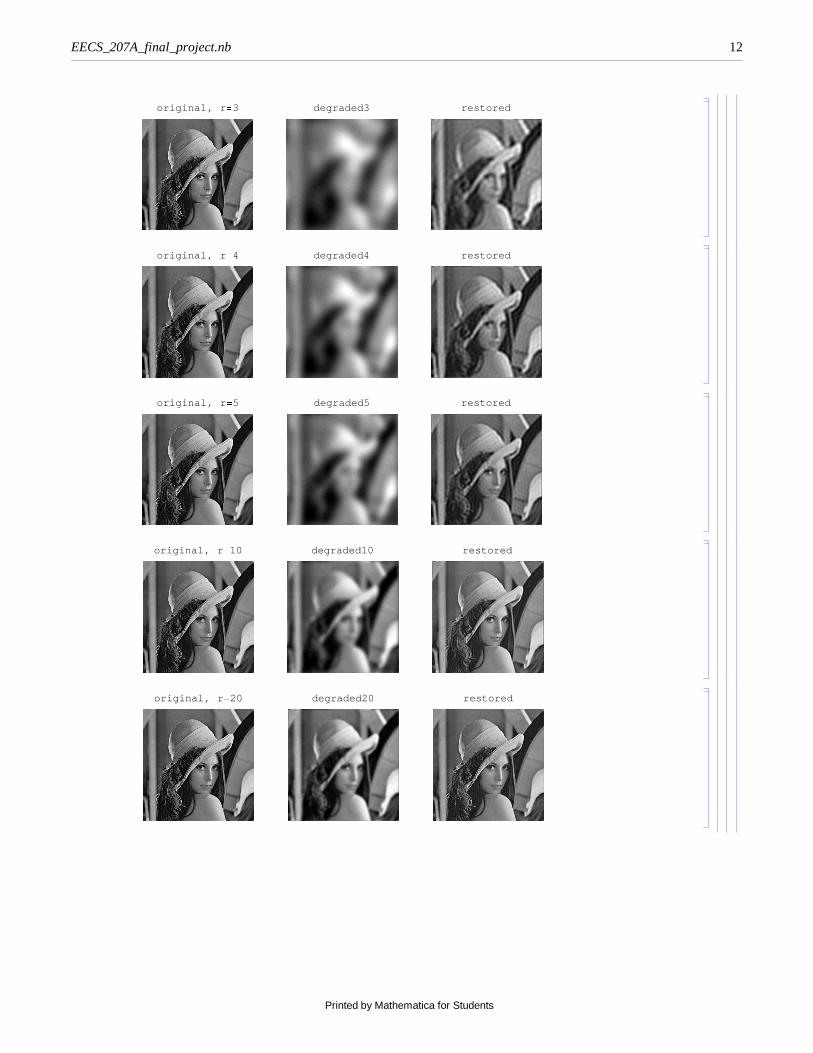
original, r =3 degraded3 restored
original, r =4 degraded4 restored
original, r =5 degraded5 restored
original, r =10 degraded10 restored
original, r =20 degraded20 restored
EECS_207A_final_project.nb 12
Printed by Mathematica for Students
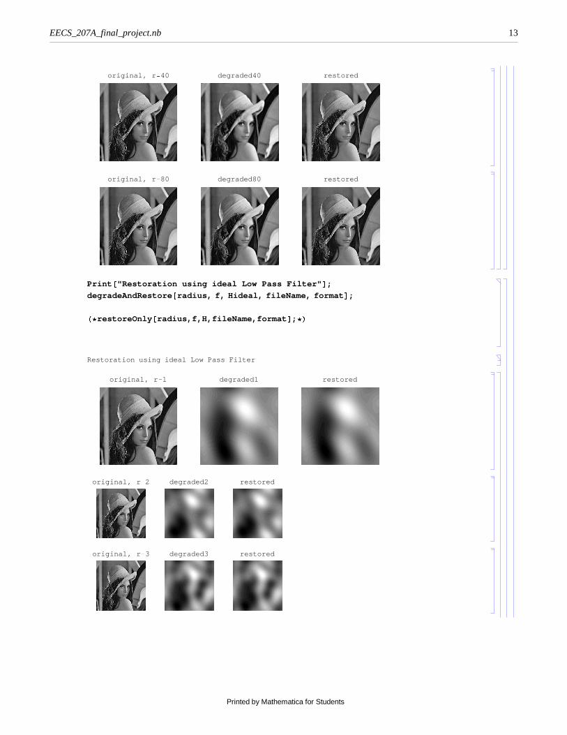
original, r =40 degraded40 restored
original, r =80 degraded80 restored
Print @"Restoration using ideal Low Pass Filter" D;
degradeAndRestore @radius, f, Hideal, fileName, format D;H∗restoreOnly @radius,f,H,fileName,format D; ∗LRestoration using ideal Low Pass Filter
original, r =1 degraded1 restored
original, r =2 degraded2 restored
original, r =3 degraded3 restored
EECS_207A_final_project.nb 13
Printed by Mathematica for Students
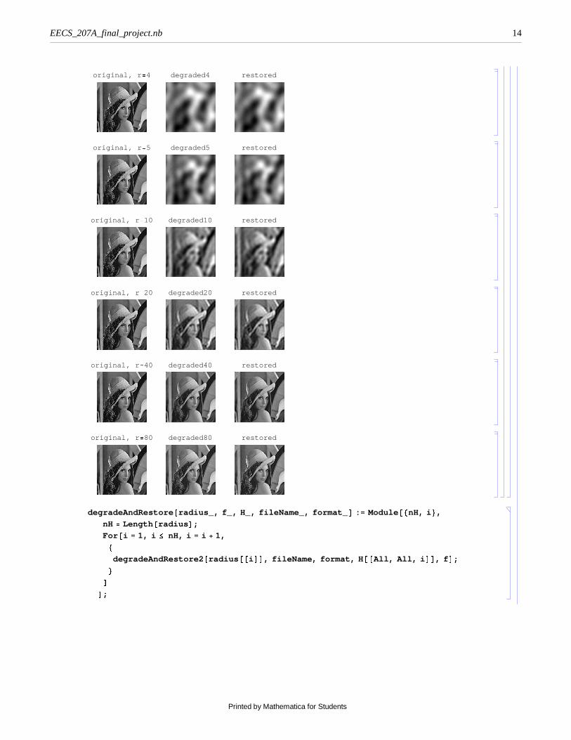
original, r =4 degraded4 restored
original, r =5 degraded5 restored
original, r =10 degraded10 restored
original, r =20 degraded20 restored
original, r =40 degraded40 restored
original, r =80 degraded80 restored
degradeAndRestore @radius_, f_, H_, fileName_, format_ D : = Module @8nH, i <,
nH = Length @radius D;
For @i = 1, i ≤ nH, i = i + 1,8degradeAndRestore2 @radius @@i DD, fileName, format, H @@All, All, i DD, f D;<DD;
EECS_207A_final_project.nb 14
Printed by Mathematica for Students
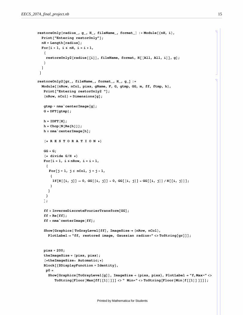
restoreOnly @radius_, g_, H_, fileName_, format_ D : = Module @8nH, i <,
Print @"Entering restorOnly" D;
nH = Length @radius D;
For @i = 1, i ≤ nH, i = i + 1,8restoreOnly2 @radius @@i DD, fileName, format, H @@All, All, i DD, g D;<DD
restoreOnly2 @gr_, fileName_, format_, H_, g_ D : =Module @8nRow, nCol, pixs, gName, F, G, gtmp, GG, m, ff, ftmp, h <,
Print @"Entering restorOnly2 " D;8nRow, nCol < = Dimensions @gD;
gtmp = nma`centerImage @gD;
G= DFT@gtmpD;
h = IDFT@HD;
h = Chop@N@Re@hDDD;
h = nma`centerImage @hD;H∗ R E S T O R A T I O N∗LGG= G;H∗ divide G êH ∗LFor @i = 1, i ≤ nRow, i = i + 1,8
For @j = 1, j ≤ nCol, j = j + 1,8If @H@@i, j DD � 0, GG@@i, j DD = 0, GG@@i, j DD = GG@@i, j DD êH@@i, j DDD;<D<D;
ff = InverseDiscreteFourierTransform @GGD;
ff = Re@ff D;
ff = nma`centerImage @ff D;
Show@Graphics @ ToGrayLevel @ff D, ImageSize → 8nRow, nCol <,
PlotLabel → "ff, restored image, Gaussian radius =" <> ToString @gr DDD;
pixs = 200;
theImageSize = 8pixs, pixs <;H∗theImageSize = Automatic; ∗LBlock @8$DisplayFunction = Identity <,
p0 =Show@Graphics @ToGrayLevel @gDD, ImageSize → 8pixs, pixs <, PlotLabel → "f,Max =" <>
ToString @Floor @Max@ff @@1DDDDD <> " Min =" <> ToString @Floor @Min@f @@1DD DDDD;
EECS_207A_final_project.nb 15
Printed by Mathematica for Students
p1 =Show@Graphics @ToGrayLevel @hDD, ImageSize → theImageSize, PlotLabel → "h, PSF" D;
gName= "g, Gaussian =" <> ToString @gr D;
p2 = Show@Graphics @ToGrayLevel @ff DD, ImageSize → theImageSize,
PlotLabel → "ff, Max =" <> ToString @Floor @Max@ff @@1DD DDD <>" Min =" <> ToString @Floor @Min@ff @@1DD DDDD;
p01 = Show@Graphics @ToGrayLevel @2 Log@1 + Abs@GDDDD,
ImageSize → theImageSize, PlotLabel → "2 Log @Abs@FD" D;
p02 = Show@Graphics @ToGrayLevel @2 Log@1 + Abs@HDDDD,
ImageSize → theImageSize, PlotLabel → "2 Log @Abs@HD" D;
p03 = Show@Graphics @ToGrayLevel @2 Log@1 + Abs@GGDDDD,
ImageSize → theImageSize, PlotLabel → "2 Log @Abs@GGD" D;D;
Show@GraphicsArray @8p0, p1, p2 <D, Frame → False D;
Show@GraphicsArray @8p01, p02, p03 <D, Frame → False D;
outFileName =fileName <> "_RESTORED_gaussian_radius_" <> ToString @gr D <> "." <> format;
ImageWrite @outFileName, ff, format DH∗Print @"Written restored image to file " <>outFileName D; ∗LD;
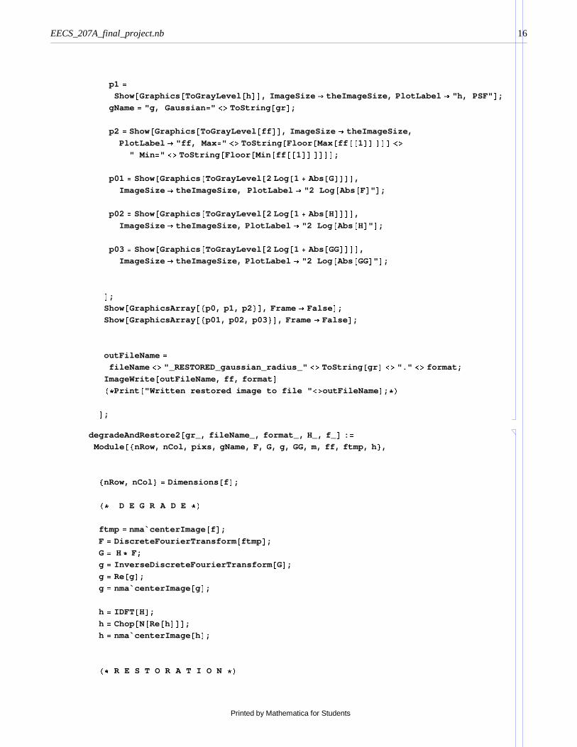
degradeAndRestore2 @gr_, fileName_, format_, H_, f_ D : =Module @8nRow, nCol, pixs, gName, F, G, g, GG, m, ff, ftmp, h <,8nRow, nCol < = Dimensions @f D;H∗ D E G R A D E∗L
ftmp = nma`centerImage @f D;
F = DiscreteFourierTransform @ftmp D;
G= H∗ F;
g = InverseDiscreteFourierTransform @GD;
g = Re@gD;
g = nma`centerImage @gD;
h = IDFT@HD;
h = Chop@N@Re@hDDD;
h = nma`centerImage @hD;H∗ R E S T O R A T I O N∗L
EECS_207A_final_project.nb 16
Printed by Mathematica for Students
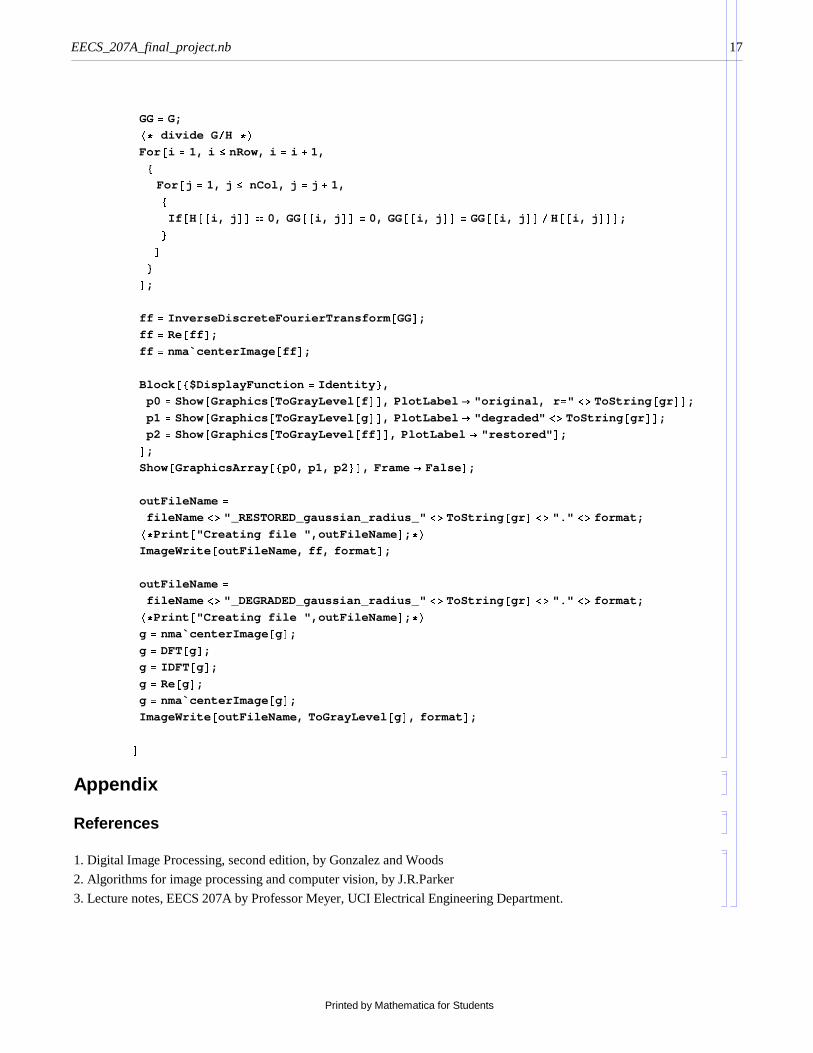
GG= G;H∗ divide G êH ∗LFor @i = 1, i ≤ nRow, i = i + 1,8
For @j = 1, j ≤ nCol, j = j + 1,8If @H@@i, j DD � 0, GG@@i, j DD = 0, GG@@i, j DD = GG@@i, j DDêH@@i, j DDD;<D<D;
ff = InverseDiscreteFourierTransform @GGD;
ff = Re@ff D;
ff = nma`centerImage @ff D;
Block @8$DisplayFunction = Identity <,
p0 = Show@Graphics @ToGrayLevel @f DD, PlotLabel → "original, r =" <> ToString @gr DD;
p1 = Show@Graphics @ToGrayLevel @gDD, PlotLabel → "degraded" <> ToString @gr DD;
p2 = Show@Graphics @ToGrayLevel @ff DD, PlotLabel → "restored" D;D;
Show@GraphicsArray @8p0, p1, p2 <D, Frame → False D;
outFileName =fileName <> "_RESTORED_gaussian_radius_" <> ToString @gr D <> "." <> format;H∗Print @"Creating file ",outFileName D; ∗L
ImageWrite @outFileName, ff, format D;
outFileName =fileName <> "_DEGRADED_gaussian_radius_" <> ToString @gr D <> "." <> format;H∗Print @"Creating file ",outFileName D; ∗L
g = nma`centerImage @gD;
g = DFT@gD;
g = IDFT@gD;
g = Re@gD;
g = nma`centerImage @gD;
ImageWrite @outFileName, ToGrayLevel @gD, format D;DAppendix
References
1. Digital Image Processing, second edition, by Gonzalez and Woods
2. Algorithms for image processing and computer vision, by J.R.Parker
3. Lecture notes, EECS 207A by Professor Meyer, UCI Electrical Engineering Department.
EECS_207A_final_project.nb 17
Printed by Mathematica for Students


![Non Linear Image Restoration in Spatial Domainsmoothing model has been used by Gabor [1], some of these techniques uses anisotropic filtering [2,3] and the neighbourhood filtering](https://img.pdfslide.us/doc/110x75/5eda1be1b3745412b570c7c5/non-linear-image-restoration-in-spatial-domain-smoothing-model-has-been-used-by.jpg)