Image Registration with Simulated Annealing and Genetic Algorithms

M A R C U S J O H A N S S O N

Master of Science Thesis Stockholm, Sweden 2006

Image Registration with Simulated Annealing and Genetic Algorithms

M A R C U S J O H A N S S O N

Master’s Thesis in Computer Science (20 credits) at the School of Computer Science and Engineering Royal Institute of Technology year 2006 Supervisor at CSC was Lars Kjelldahl Examiner was Lars Kjelldahl TRITA-CSC-E 2006:030 ISRN-KTH/CSC/E--06/030--SE ISSN-1653-5715 Royal Institute of Technology School of Computer Science and Communication KTH CSC SE-100 44 Stockholm, Sweden URL: www.csc.kth.se

Abstract

Image Registration with Simulated Annealing and Genetic Algorithms

Image registration is the process of finding correspondence between two images depicting aparticular scene. This thesis evaluates the use of genetic algorithms and simulated anneal-ing to perform image registration in the context of image stitching. Being metaheuristics,these optimization techniques require several decisions to be made during implementation.For genetic algorithms, solution encoding and evolutionary operators are evaluated withrespect to performance on some image registration problems. For simulated annealing,suitable neighborhood generators are evaluated, together with an analysis of suitable stop-ping criteria and cooling schemes. In addition, a few improvements to the original heuristicsare proposed and evaluated. Results indicate that the investigated optimization techniquesindeed can be used to perform image registration efficiently, the main weakness howeverbeing the need for problem specific adjustments to achieve the best performance.

Sammanfattning

Bildregistrering med simulerad avkylning och genetiska algoritmer

Detta exjobb utvärderar användandet av genetiska algoritmer och simulerad avkylning somoptimeringsmetoder för problemet att sammanfoga mindre bilder av ett motiv till en störresammansatt bild (eng. image registration). Som metaheuristiker kräver dessa metoder ettflertal beslut under implementering. För genetiska algoritmer testades några olika lösnings-kodningar samt evolutionära operatorer med hänseende till prestanda på några samman-fogningsproblem. För simulerad avkylning jämfördes och utvärderades några generatorerav närliggande lösningar, samt avkylningsscheman och stoppkriteria. Utöver detta föreslåsoch utvärderades några förbättringar till de ursprungliga metoderna. Resultaten indikeraratt de utvärderade optimeringsteknikerna kan användas för effektiv bildsammanfogning,men att problemspecifik finjustering av metoderna kan vara nödvändig för att uppnå bästaprestanda.

For dad, I miss you.

Foreword and Acknowledgements

This report was produced as part of a Master’s Thesis conducted at the Schoolof Computer Science and Communication at the Royal Institute of Technology inStockholm, Sweden. My thanks goes to everyone that in one way or the other helpedme during my work with the thesis. In particular, I would like to thank MarcusHoverby at Révolte Developement for his support and pleasant company. Thanksalso to my supervisor and examiner Lars Kjelldahl for helping me with practicalissues related to the work as well as giving invaluable advice and tutoring.

Marcus Johansson, March 2006

v

Contents

Foreword and Acknowledgements v

1 Introduction 11.1 Problem Description . . . . . . . . . . . . . . . . . . . . . . . . . . . 11.2 Goals . . . . . . . . . . . . . . . . . . . . . . . . . . . . . . . . . . . 21.3 Limitations . . . . . . . . . . . . . . . . . . . . . . . . . . . . . . . . 21.4 Organization . . . . . . . . . . . . . . . . . . . . . . . . . . . . . . . 2

2 Background 32.1 Image Acquisiton . . . . . . . . . . . . . . . . . . . . . . . . . . . . . 32.2 Preprocessing . . . . . . . . . . . . . . . . . . . . . . . . . . . . . . . 42.3 Registration . . . . . . . . . . . . . . . . . . . . . . . . . . . . . . . . 5

2.3.1 Features . . . . . . . . . . . . . . . . . . . . . . . . . . . . . . 62.3.2 Similarity Measures . . . . . . . . . . . . . . . . . . . . . . . 62.3.3 Search Set . . . . . . . . . . . . . . . . . . . . . . . . . . . . . 82.3.4 Search Strategies . . . . . . . . . . . . . . . . . . . . . . . . . 10

2.4 Merging . . . . . . . . . . . . . . . . . . . . . . . . . . . . . . . . . . 122.4.1 Measuring Quality . . . . . . . . . . . . . . . . . . . . . . . . 14

3 Optimization Theory 153.1 Search Space . . . . . . . . . . . . . . . . . . . . . . . . . . . . . . . 153.2 Genetic Algorithms . . . . . . . . . . . . . . . . . . . . . . . . . . . . 15

3.2.1 Background . . . . . . . . . . . . . . . . . . . . . . . . . . . . 163.2.2 Algorithm Description . . . . . . . . . . . . . . . . . . . . . . 163.2.3 Stopping Criteria . . . . . . . . . . . . . . . . . . . . . . . . . 193.2.4 Genetic Algoritms and Image Registration . . . . . . . . . . . 20

3.3 Simulated Annealing . . . . . . . . . . . . . . . . . . . . . . . . . . . 203.3.1 Background . . . . . . . . . . . . . . . . . . . . . . . . . . . . 203.3.2 Algorithm Description . . . . . . . . . . . . . . . . . . . . . . 213.3.3 Simulated Annealing and Image Registration . . . . . . . . . 23

4 Method 254.1 Choice of Method . . . . . . . . . . . . . . . . . . . . . . . . . . . . . 254.2 Conditions and Limitations . . . . . . . . . . . . . . . . . . . . . . . 26

4.3 Experimental Setting . . . . . . . . . . . . . . . . . . . . . . . . . . . 264.3.1 Images . . . . . . . . . . . . . . . . . . . . . . . . . . . . . . . 264.3.2 Preprocessing . . . . . . . . . . . . . . . . . . . . . . . . . . . 274.3.3 State Representation . . . . . . . . . . . . . . . . . . . . . . . 274.3.4 Sampling . . . . . . . . . . . . . . . . . . . . . . . . . . . . . 27

4.4 Performance Evaluation and Comparison . . . . . . . . . . . . . . . 284.5 Genetic Algorithms . . . . . . . . . . . . . . . . . . . . . . . . . . . . 28

4.5.1 Limitations . . . . . . . . . . . . . . . . . . . . . . . . . . . . 294.5.2 Tested Parameters . . . . . . . . . . . . . . . . . . . . . . . . 294.5.3 Proposed Enhancements . . . . . . . . . . . . . . . . . . . . . 30

4.6 Simulated Annealing . . . . . . . . . . . . . . . . . . . . . . . . . . . 324.6.1 Initial Temperature . . . . . . . . . . . . . . . . . . . . . . . 324.6.2 Neighborhood Generation . . . . . . . . . . . . . . . . . . . . 324.6.3 Cooling Rates and Chain Lengths . . . . . . . . . . . . . . . 354.6.4 Stopping Criteria . . . . . . . . . . . . . . . . . . . . . . . . . 354.6.5 Proposed Enhancement . . . . . . . . . . . . . . . . . . . . . 35

4.7 Implementation . . . . . . . . . . . . . . . . . . . . . . . . . . . . . . 354.7.1 Environment . . . . . . . . . . . . . . . . . . . . . . . . . . . 354.7.2 Program Structure . . . . . . . . . . . . . . . . . . . . . . . . 354.7.3 Other Issues . . . . . . . . . . . . . . . . . . . . . . . . . . . . 36

5 Experimental Results 375.1 Basic Implementation . . . . . . . . . . . . . . . . . . . . . . . . . . 375.2 Genetic Algorithm . . . . . . . . . . . . . . . . . . . . . . . . . . . . 38

5.2.1 Search Space Signature . . . . . . . . . . . . . . . . . . . . . 385.2.2 Encoding and Operators . . . . . . . . . . . . . . . . . . . . . 405.2.3 Enhancements . . . . . . . . . . . . . . . . . . . . . . . . . . 415.2.4 Convergence and Stopping Criteria . . . . . . . . . . . . . . . 435.2.5 Population Size . . . . . . . . . . . . . . . . . . . . . . . . . . 435.2.6 Summary . . . . . . . . . . . . . . . . . . . . . . . . . . . . . 44

5.3 Simulated Annealing . . . . . . . . . . . . . . . . . . . . . . . . . . . 455.3.1 Search Space Signature . . . . . . . . . . . . . . . . . . . . . 455.3.2 Neighborhood Generation . . . . . . . . . . . . . . . . . . . . 455.3.3 Further Analysis . . . . . . . . . . . . . . . . . . . . . . . . . 465.3.4 Summary . . . . . . . . . . . . . . . . . . . . . . . . . . . . . 48

5.4 Comparisons . . . . . . . . . . . . . . . . . . . . . . . . . . . . . . . 48

6 Conclusions 516.1 Summary . . . . . . . . . . . . . . . . . . . . . . . . . . . . . . . . . 516.2 Further Work . . . . . . . . . . . . . . . . . . . . . . . . . . . . . . . 52

Bibliography 53

List of Tables

4.1 Program Components . . . . . . . . . . . . . . . . . . . . . . . . . . . . 36

5.1 Performance of the best runs of different GA operators . . . . . . . . . . 425.2 Performance of the best runs of VAL12 and enhanced operators . . . . . 435.3 Distinct states visited at 0-error enhanced GA operators at different

populations . . . . . . . . . . . . . . . . . . . . . . . . . . . . . . . . . . 455.4 Performance of the best runs of different neighborhood generators . . . 465.5 Results of Norr Mälarstrand stitching batch . . . . . . . . . . . . . . . . 50

List of Figures

2.1 Stages in image stitching . . . . . . . . . . . . . . . . . . . . . . . . . . 32.2 Geometrical transformations . . . . . . . . . . . . . . . . . . . . . . . . 82.3 Automatically selected sub-image blocks shown as brighter squares . . . 10

3.1 Cost function landscape generated from a 2D search space . . . . . . . . 163.2 Genetic algorithm control flow . . . . . . . . . . . . . . . . . . . . . . . 173.3 Roulette wheel selection . . . . . . . . . . . . . . . . . . . . . . . . . . . 183.4 Simulated snnealing control flow . . . . . . . . . . . . . . . . . . . . . . 22

5.1 Pictures with matched areas marked . . . . . . . . . . . . . . . . . . . . 385.2 Final result after merging . . . . . . . . . . . . . . . . . . . . . . . . . . 385.3 Search space signatures with binary encoding and 1p and 2p crossover

operators (BIN1 and BIN2) over 100 generations, popsize = 49, pcrossover =0.8, pmutation = 0.4 . . . . . . . . . . . . . . . . . . . . . . . . . . . . . . 39

5.4 Search space signatures with value encoding and crossover operatorsVAL11 and VAL21 over 100 generations, popsize = 49, pcrossover = 0.8,pmutation = 0.4 . . . . . . . . . . . . . . . . . . . . . . . . . . . . . . . . 40

5.5 Search space signatures with value encoding and crossover operatorsVAL21 and VAL22 over 100 generations, popsize = 49, pcrossover = 0.9,pmutation = 0.4 . . . . . . . . . . . . . . . . . . . . . . . . . . . . . . . . 40

5.6 Error rates of different operator configurations over 250 generations . . 415.7 Error rate of VAL12 and enhanced configurations over 250 generations . 425.8 Convergence of the best VAL12, VAL12-N, VAL12-D and VAL12-ND

operators . . . . . . . . . . . . . . . . . . . . . . . . . . . . . . . . . . . 445.9 Simulations with COR, M = 40, α = 0.95 and AAN, M = 30, α = 0.90,

pstop = 0.10 . . . . . . . . . . . . . . . . . . . . . . . . . . . . . . . . . . 465.10 Error of TMP neighborhood generator plotted against cooling rate and

chain length, pstop = 0.01 . . . . . . . . . . . . . . . . . . . . . . . . . . 475.11 Converge of COR runs at α = 0.75 and α = 0.97 . . . . . . . . . . . . . 475.12 Six overlapping images . . . . . . . . . . . . . . . . . . . . . . . . . . . . 485.13 View from Norr Mälarstrand 24, Stockholm, Sweden. Final stitch cre-

ated from 6 images. . . . . . . . . . . . . . . . . . . . . . . . . . . . . . 50

Chapter 1

Introduction

This report describes my Master’s Thesis work made at the School of ComputerScience and Communication, Royal Institute of Technology, Sweden. The work iscommissioned by Révolte Development AB, a Swedish company developing soft-ware for digital image management and manipulation. The company is located inStockholm where the main part of the work related to this thesis was conducted.

1.1 Problem Description

Image stitching is the process of creating high resolution panorama pictures fromseveral partly overlapping digital pictures. With the increased popularity of digitalcameras, this is an interesting concept not only to the professional graphics artistbut also to the consumer. Image stitching methods have application in other areasof digital photo management as well, helping to reduce compression artefacts inphotographs and creating image mosaics. A crucial part when performing imagestitching is to superimpose two images and find an optimal match by transformingone of them through e.g. alignment, rotation and scaling. This process is calledregistration, and aims at fitting the images together in the most visually pleasingway without unnecessarily obscuring the photometry of the original images. Imageregistration has in addition to stitching application in such diverse areas as themerging of satellite photos and brain scan images. The registration process can berather computationally intensive, why the use of efficient registration methods is ofmajor concern.

1

1.2 Goals

Quite extensive research has been conducted by the scientific community within thearea of image stitching and registration, and today’s state of the art methods pro-duce impressive results. This thesis focus on image registration through simulatedannealing (SA) and genetic algorithms (GA), two stochastic optimization methodsthat this far have not gained much attention in this particular field of work. Theoptimization strategies are metaheuristic, leaving many choices and decisions to bemade during implementation. The investigation aims at resolving suitable paramet-rical choices for efficient image registration in terms of low error and high speed.These choices should as far as possible be general enough to apply to a varietyof common image registration tasks stemming from image stitching of consumerphotographs.

1.3 Limitations

The thesis will primarily concern the registration of images, and only shallowly touchother areas in the image stitching process such as image preprocessing and seamremoval. The thesis will not concern so called automatic image registration, whereimages are given to registration in an unordered fashion, leaving for the computerto deduce which images should be superimposed and how.

1.4 Organization

The report is organized as follows. The second chapter is a literature review of thearea that gives the reader some theoretical field background on the image stitchingprocess. The third chapter reviews the SA and GA optimization methods andsome of the research made on them concerning image registration. The fourthchapter focuses on experimental method and implementation issues. Results fromthe investigation are presented in the fifth chapter. The sixth and last chaptercontains conclusions drawn and gives some guidelines on potential future work inthe area.

2

Chapter 2

Background

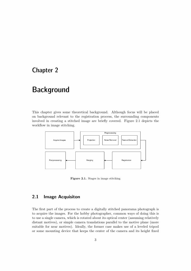
This chapter gives some theoretical background. Although focus will be placedon background relevant to the registration process, the surrounding componentsinvolved in creating a stitched image are briefly covered. Figure 2.1 depicts theworkflow in image stitching.

Figure 2.1. Stages in image stitching

2.1 Image Acquisiton

The first part of the process to create a digitally stitched panorama photograph isto acquire the images. For the hobby photographer, common ways of doing this isto use a single camera, which is rotated about its optical center (assuming relativelydistant motives), or simple camera translations parallel to the motive plane (moresuitable for near motives). Ideally, the former case makes use of a leveled tripodor some mounting device that keeps the center of the camera and its height fixed

3

during rotation. The latter case is harder to perform by hand, since it requiresall images to lie in the same plane to produce accurate results. Also, translationsdo not produce the three-dimensional feeling obtained by stitching images acquiredthrough rotation.

The amount of overlap between adjacent images affects the quality of the stitchedimage. Chen [5] suggests 50% overlap with the previous image and 50% overlapwith the following image. In case of camera rotations, this overlap ratio depends onthe rotation angle between successive images. A relatively large overlap is especiallyimportant when the camera is hand held, since this implies limited unwanted trans-lations and rotations. We will not delve deeper into various acquisition methodshere, Gledhill [8] holds a detailed account for the interested reader.

Manual acquisition of images of a live scene inevitably produces problems that willneed to be addressed in later stages of the stitching process. The quality of thefinal composite is greatly dependent on the setting and methods used to acquire theimages, main problems include:

• Intensity shifts between adjacent images due to variations in lighting con-ditions.

• Reflective regions and moving objects changes the appearance of objectsbetween adjacent images, which makes the registration process more difficult.

• Varying degrees of lens distortion might appear depending on the lens used.This can be corrected by using the same lens to take an image of a grid, andthrough known grid properties calculate the properties of the distortion andthe transformation needed to recover it [5].

2.2 Preprocessing

Before starting the image registration process, a preprocessing step may increasethe probability of a successful registration and enhance the end result.

As pictures are taken, objects from the real world are projected onto the 2D planeof the images. Since the orientation between each imaging plane is different (as-suming acquisition by rotation, with or without tilting of the camera), we need tomathematically define how pixel coordinates from one image will map into the co-ordinates of our final stitched image world. A parametric motion model does this,and which is used depends on what we know about the photographs and how theywere acquired.

4

Given a set of images acquired with rotation about the fixed centre of a level camera,one approach is to project the images onto a common cylindrical surface. Once thisis done, pure translational transforms suffice to align the images correctly [17]. Themapping from world coordinates (X, Y, Z) to 2D cylindrical coordinates (θ, v) isgiven by equations 2.1) and 2.2.

θ = tan−1(X/Z) (2.1)

v =Y√

X2 + Y 2(2.2)

In order to project the images, we sweep through all the coordinates in our projec-tion and see where the ”projection beam” falls in the original image plane. We needto account for that some beams may fall outside our original image, and prepare tointerpolate where the beam hits pixels at fractional coordinates. Images acquiredwith various degrees of camera tilt require mapping to spherical coordinates beforealignment, we will however not expand on that further here.

Before aligning the overlapping images, it is suitable to reduce noise in the images.Depending on the noise to remove, various filters may be suitable. A common multi-purpose smoothing filter is the 2D gaussian smoothing filter kernel, its discreteversion shown below (equation 2.3).

G(x, y) =1√2πσ

e−(x2+y2)

2σ2 (2.3)

where σ2 is the variance of the blur, controlling the amount of smoothing applied.A nice property of the Gaussian is that it is decomposable and can be applied onedimension at a time in series, which reduces time complexity.

If the noise is distinct and spread out, a median filter reduces noise without blurringsharp edges and loosing detail. For detailed information on noise reduction andsmoothing filters, see Gonzalez [9].

2.3 Registration

Once the images are transformed into a common motion model, we need a way tofind how they can be made to fit together in the most visually pleasing way. Thisprocess of aligning the overlapping images is known as registration. During theprocedure, one image is fixed (the reference image), and the other (the input image)

5

is transformed to become similar to the reference image in the area of overlapping.The transformations should by applied so as to reduce the amount of impact on thequality and photometry of the original images. A registration algorithm typicallyutilizes four different components:

• Image features are elements of the images that are used in the alignmentprocess. They may be pixel intensity values, in which case the registrationmethod is referred to as direct, or other characteristics and interest points ofthe images.

• The similarity measure (also referred to as cost, score, energy or fitness) isa scalar indication of the similarity between two features from the images tobe aligned. The scalar value guides the algorithm on suitable transformations.

• The search set defines the set of transformations (translations, rotations,etcetera) available during the registration process.

• The search strategy defines how the search for an optimal or near optimalalignment of the images in terms of the similarity measure is carried out, byselecting the next transformation to be carried out from the search set.

2.3.1 Features

The simplest and most straightforward feature set is the image pixel intensity values.The major drawback of this approach is that average intensity differences betweenthe images make similarity comparisons skewed. A good alternative that is more orless insensitive to average intensity differences is the edge set of an image. Edgesoften convey vital information in the image, and may make a suitable feature set.

Numerous methods exist to obtain a binary edge map. Convolution with Laplacian,Sobel or Prewitt operators are common and straightforward approaches. More elab-orate and computationally intensive methods include the Hough Transform1.

2.3.2 Similarity Measures

The similarity measure function, or cost function, gives an indication of the sim-ilarity between two compared image regions. The function may either be basedon direct pixel intensity comparisons, or on other geometrical features within theregions. In this thesis, focus is put on direct intensity comparisons. Three of theseare described below.

1See [9] for a detailed account

6

Sum of Squared Differences

A simple similarity measure is the sum of the differences between compared pixelintensities within the area, squared. In case of color photographs we may lookat each color channel separately and take the average. Equation 2.4 defines thefunction, known as SSD (Sum of Squared Differences) mathematically.

ESSD(h, k) =h∑i

w∑j

(I1(i + h, j + k)− I0(i, j))2 (2.4)

where Ii denotes the intensity value at image i, and h, k defines the offset point inthe input image for which the similarity measure should be calculated. The mainweakness of this measure is that intensity shifts between the images may causelarge differences even at the most optimal matching position, potentially leading toinaccurate results and misalignment.

Normalized Cross Correlation

Cross Correlation (equation 2.5) is a method to measure the similarity between twosignals by summing over the products of aligned pixels. The measure is usuallynormalized to reduce the effect of local regions with high intensities.

ENCC(u) =∑

i

I0(xi)I1(xi + u) (2.5)

where u is a vector defining the offset between the pictures in pixels.

Variance

Another similarity measure is to look at the standard deviation of the intensitydifferences of the compared region. This approach is less susceptible to failure dueto intensity shifts than squared differences, since the intensity difference should be ofapproximately the same amount for each compared pixel, resulting in small varianceand standard deviation. Equation 2.6 gives a variance based similarity measure atoffset (h, k).

EV (h, k) =√

V ar(Idiff (h, k)) (2.6)

7

where Idiff is the set of intensity differences within the compared region.

It may also be possible to improve results by utilizing spatially varying weights orbiases to compensate for mean intensity variations between the images [17].

2.3.3 Search Set

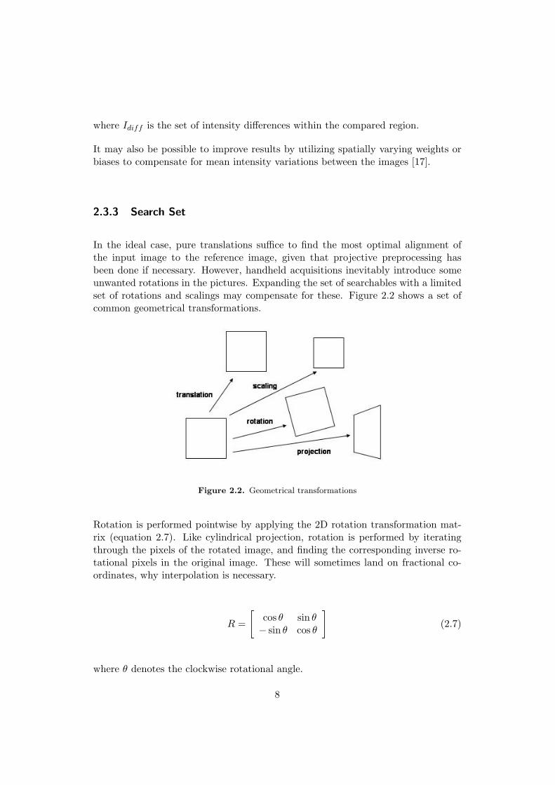
In the ideal case, pure translations suffice to find the most optimal alignment ofthe input image to the reference image, given that projective preprocessing hasbeen done if necessary. However, handheld acquisitions inevitably introduce someunwanted rotations in the pictures. Expanding the set of searchables with a limitedset of rotations and scalings may compensate for these. Figure 2.2 shows a set ofcommon geometrical transformations.

Figure 2.2. Geometrical transformations

Rotation is performed pointwise by applying the 2D rotation transformation mat-rix (equation 2.7). Like cylindrical projection, rotation is performed by iteratingthrough the pixels of the rotated image, and finding the corresponding inverse ro-tational pixels in the original image. These will sometimes land on fractional co-ordinates, why interpolation is necessary.

R =

[cos θ sin θ− sin θ cos θ

](2.7)

where θ denotes the clockwise rotational angle.

8

Sub-pixel Registration

Technically, nothing prevents the search from being done with fractional resolution,in which case we need to be able to interpolate between neighboring pixel intensities.A number of interpolation methods exist, bilinear interpolation being a popularalternative. Other interpolation methods based on other than pixel intensities exist,but generally performs weaker than intensity-based interpolation [3]. In general,however, errors of ±1 pixels from the optimal is considered acceptable.

Automatic Sub-image Selection

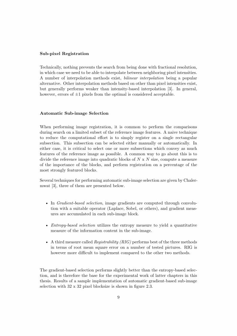
When performing image registration, it is common to perform the comparisonsduring search on a limited subset of the reference image features. A naive techniqueto reduce the computational effort is to simply register on a single rectangularsubsection. This subsection can be selected either manually or automatically. Ineither case, it is critical to select one or more subsections which convey as muchfeatures of the reference image as possible. A common way to go about this is todivide the reference image into quadratic blocks of N x N size, compute a measureof the importance of the blocks, and perform registration on a percentage of themost strongly featured blocks.

Several techniques for performing automatic sub-image selection are given by Chaler-mwat [3], three of them are presented below.

• In Gradient-based selection, image gradients are computed through convolu-tion with a suitable operator (Laplace, Sobel, or others), and gradient meas-ures are accumulated in each sub-image block.

• Entropy-based selection utilizes the entropy measure to yield a quantitativemeasure of the information content in the sub-image.

• A third measure called Registrability (RIG) performs best of the three methodsin terms of root mean square error on a number of tested pictures. RIG ishowever more difficult to implement compared to the other two methods.

The gradient-based selection performs slightly better than the entropy-based selec-tion, and is therefore the base for the experimental work of latter chapters in thisthesis. Results of a sample implementation of automatic gradient-based sub-imageselection with 32 x 32 pixel blocksize is shown in figure 2.3.

9

Figure 2.3. Automatically selected sub-image blocks shown as brighter squares

2.3.4 Search Strategies

The search strategy governs how the search space is explored, and has a greatimpact on the efficiency of the image registration process. Here we review a fewcommon strategies, leaving the genetic algorithm and simulated annealing to a morethorough account in the next chapter.

Exhaustive Search

A simple exhaustive search (or full search) where all states of the search spaceare computed, is guaranteed to find the optimal alignment. However, keeping inmind that similarity measure computation usually has complexity on the orderof the number of pixels in the compared areas, this is a rather computationallyintensive and time consuming strategy, which quickly becomes infeasible to applyon everything but very limited search sets and spaces.

10

Step Search

A faster alternative to the exhaustive search is the step search strategy. Variousbrands of this strategy exist, the basis however being a method that iterativelyconverges towards the optimal alignment with logarithmic order complexity. Ineach iteration, a center point is defined, and four points are selected at an equal stepdistance from this point towards north, south, west and east. Similarity measuresare calculated for the four points and the center point, and the best point forms thecenter point of the next iteration that starts with half the previous step distance.This quickly converges towards a minimum point. Unfortunately, the method issusceptible to trap itself around a local optimum and miss the global one, resultingin misalignment. Chen [5] suggests that the method is used to make fast estimationsof the optimal position.

Gradient Descent

Another approach is to perform gradient descent on an appropriate similarity meas-ure function. Gradient descent works by calculating the gradient at the currentpoint, and iteratively move in the negative gradient direction (in case minimiza-tion of the similarity measure is our objective). Obviously, the method requires adifferentiable and rather smooth objective function surface.

A parameter γ called the learning rate affects how great the leap in the negativegradient direction should be. The initial learning rate must be suited to fit theobjective function. A high learning rate makes faster convergence possible, butintroduces the risk of ”shooting over the target” by causing moves that passes overthe minima valley and worsens the similarity measure. Because of this, the learningrate is usually decreased when a step in the negative gradient direction does notresult in a better similarity measure. Adaptive approaches do this, and also makea small increase on the learning rate if a step results in a better similarity measure.

Gradient descent requires an initial starting point on the function, which is usuallyrandomly selected.

Multi-resolution Search

In multi-resolution (or subpixel) image registration, the search space is reduced bysearching at different resolutions in an hierarchical manner. The search is madeon a set of down sampled versions of the original images, and matches are iterat-

11

ively refined at higher resolutions. The concept of image wavelet2 decompositionhas successfully been put to use in multi-resolution registration. A wavelet-basedtechnique called the iterative refinement algorithm (IRA) combined with a geneticalgorithm-based search strategy have proven to give accurate and fast results [4].

2.4 Merging

When the registration process is completed and an alignment has been found, theimages rarely fit together in a way that is immediately visually pleasing. This is dueto acquisition conditions and misregistration. The post processing step of mergingaims to make the transition between the images invisible while preserving as muchof the quality and originality of the images as possible.

Different approaches to merging exist. One way is to let both overlapping pixels in-fluence the result of the final composite pixel according to some specific weightening.The major drawback of this is low resulting contrast and potential ghosting 3 arti-facts in case of misalignment. Another approach is to divide the overlapping regionin two halves at the centre and let each image contribute with one half. This usuallyproduces a visible seam that must be removed. Other methods change the imagesat a global level (outside the overlapping region) to produce better composites,or create meandering seams that fuse the images where their intensity differencesare minimal (optimal seam algorithms). While the major concern of this thesis isefficient registration, only a few methods are discussed briefly below.

Feathering and Pyramid Blending

A rather simple and reasonable approach to merging is to let overlapping pixelscontribute to the final composite with weighting inversely proportional to the dis-tance to the image center, a method often referred to as feathering. Hence a pixelfar away from the image center will contribute less to the final composite than apixel near the image center.

Another variation on the same theme is pyramid blending where low frequencydetails are mixed over a wire neighborhood around the seam, and high frequencydetails are mixed narrowly around the seam. The result is gradual transitions in

2See Gonzalez [9]3When the final registration suggest to merge the images so that an object in one of the images

do not appear on the corresponding offset in the other image, the object will appear less intenseand shade-like in the final composite, hence the term ghosting.

12

smooth low frequency regions, and a reduced amount of edge duplications in highfrequency regions.

Linear Distribution of Differences

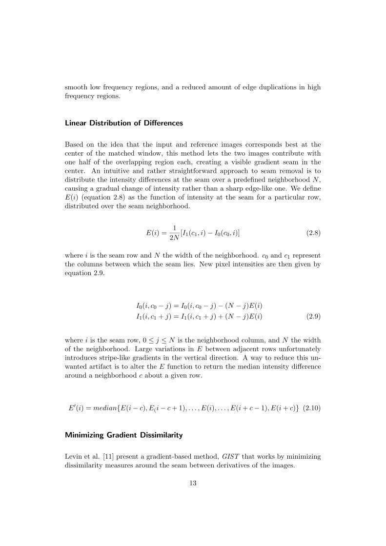
Based on the idea that the input and reference images corresponds best at thecenter of the matched window, this method lets the two images contribute withone half of the overlapping region each, creating a visible gradient seam in thecenter. An intuitive and rather straightforward approach to seam removal is todistribute the intensity differences at the seam over a predefined neighborhood N ,causing a gradual change of intensity rather than a sharp edge-like one. We defineE(i) (equation 2.8) as the function of intensity at the seam for a particular row,distributed over the seam neighborhood.

E(i) =1

2N[I1(c1, i)− I0(c0, i)] (2.8)

where i is the seam row and N the width of the neighborhood. c0 and c1 representthe columns between which the seam lies. New pixel intensities are then given byequation 2.9.

I0(i, c0 − j) = I0(i, c0 − j)− (N − j)E(i)I1(i, c1 + j) = I1(i, c1 + j) + (N − j)E(i) (2.9)

where i is the seam row, 0 ≤ j ≤ N is the neighborhood column, and N the widthof the neighborhood. Large variations in E between adjacent rows unfortunatelyintroduces stripe-like gradients in the vertical direction. A way to reduce this un-wanted artifact is to alter the E function to return the median intensity differencearound a neighborhood c about a given row.

E′(i) = median{E(i− c), E(i− c + 1), . . . , E(i), . . . , E(i + c− 1), E(i + c)} (2.10)

Minimizing Gradient Dissimilarity

Levin et al. [11] present a gradient-based method, GIST that works by minimizingdissimilarity measures around the seam between derivatives of the images.

13

2.4.1 Measuring Quality

In addition to visual inspection, it is desirable to quantify the quality of the end-result of an image stitching implementation.

A commonly used method is to measure the similarity of the final result to theoriginal pictures at a pixel-to-pixel basis. Another measurement is to evaluate thecontrast of the final result in terms of intensity differences between neighboringpixels. In the case merging is performed with a seam-based method, the area inclose vicinity to the seam is of particular interest.

14

Chapter 3

Optimization Theory

This chapter reviews the theory behind the optimization methods Simulated An-nealing and Genetic Algorithms. Some research regarding the implementation ofthe methods on image registration is reviewed.

3.1 Search Space

When solving an image registration problem, we look for a particular solution thatwill be better than all or almost all other feasible solutions. Depending on thenumber of parameters n that constitute a solution, an n-dimensional search spaceconsisting of the set of all possible solutions is created. If we mark each point in thesearch space with the corresponding cost for that solution, we get a landscape-likehypersurface. Our aim with the search is to find the lowest valley in this landscape.This is often a rather time consuming process, since the hypersurface rarely behavesin a smooth and predictable way.

Figure 3.1 shows an interpolated mesh of a landscape generated from a typical imageregistration problem instance. As can be seen, the cost function landscape is filledwith local minima. Note though that the global minimum resides at a much deeperlevel than the average local minima.

3.2 Genetic Algorithms

This section describes the Genetic Algorithm (GA), a random optimization tech-nique inspired by the theory of evolution and the survival of the fittest. Genetic

15

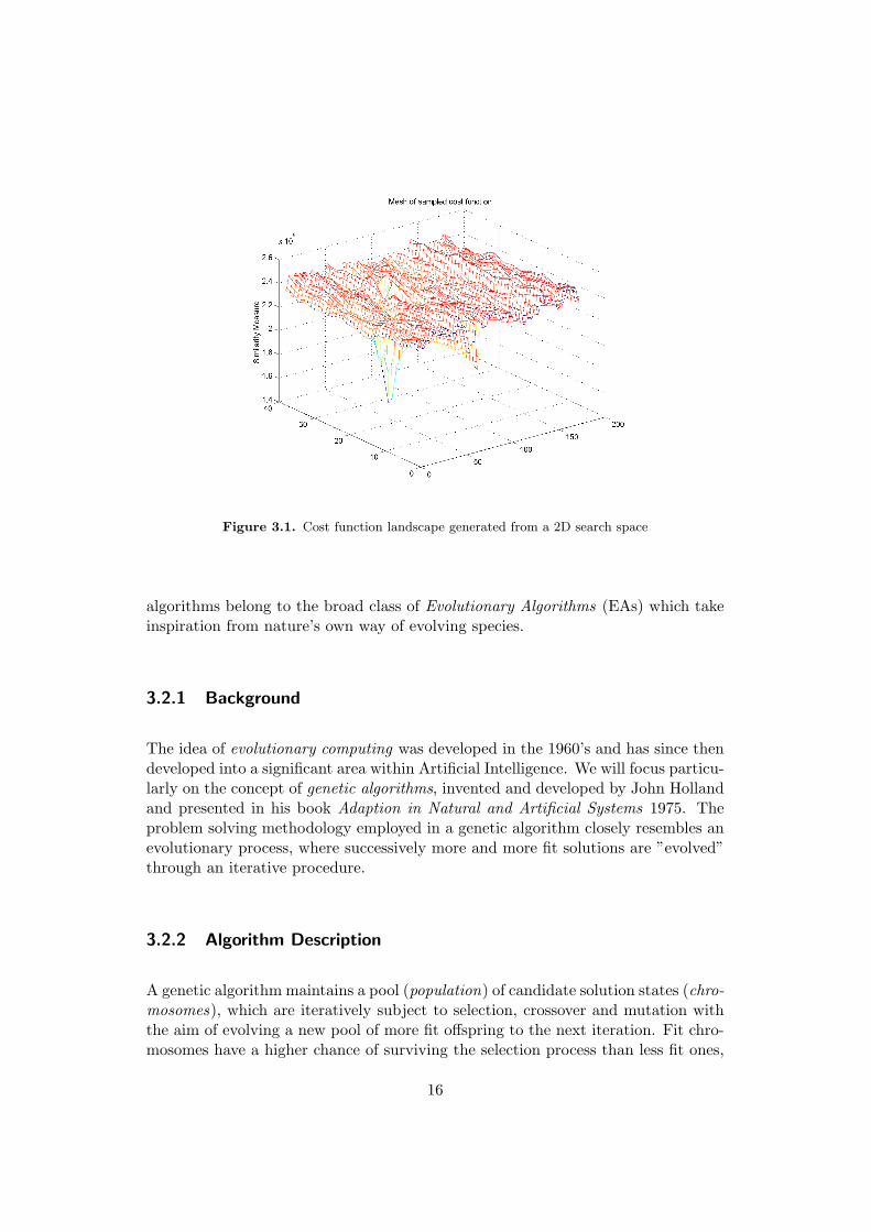
Figure 3.1. Cost function landscape generated from a 2D search space

algorithms belong to the broad class of Evolutionary Algorithms (EAs) which takeinspiration from nature’s own way of evolving species.

3.2.1 Background

The idea of evolutionary computing was developed in the 1960’s and has since thendeveloped into a significant area within Artificial Intelligence. We will focus particu-larly on the concept of genetic algorithms, invented and developed by John Hollandand presented in his book Adaption in Natural and Artificial Systems 1975. Theproblem solving methodology employed in a genetic algorithm closely resembles anevolutionary process, where successively more and more fit solutions are ”evolved”through an iterative procedure.

3.2.2 Algorithm Description

A genetic algorithm maintains a pool (population) of candidate solution states (chro-mosomes), which are iteratively subject to selection, crossover and mutation withthe aim of evolving a new pool of more fit offspring to the next iteration. Fit chro-mosomes have a higher chance of surviving the selection process than less fit ones,

16

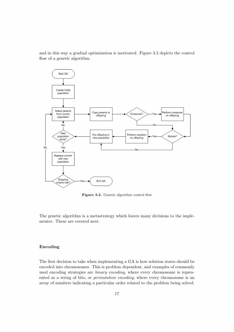
and in this way a gradual optimization is motivated. Figure 3.2 depicts the controlflow of a genetic algorithm.

Figure 3.2. Genetic algorithm control flow

The genetic algorithm is a metastrategy which leaves many decisions to the imple-menter. These are covered next.

Encoding

The first decision to take when implementing a GA is how solution states should beencoded into chromosomes. This is problem dependent, and examples of commonlyused encoding strategies are binary encoding, where every chromosome is repres-ented as a string of bits, or permutation encoding, where every chromosome is anarray of numbers indicating a particular order related to the problem being solved.

17

Selection

The best selection strategy for picking the parents to be the base for new offspringchromosomes is often problem specific. All strategies should however reflect thebasic idea that a higher fitness means a higher likelihood of being selected.

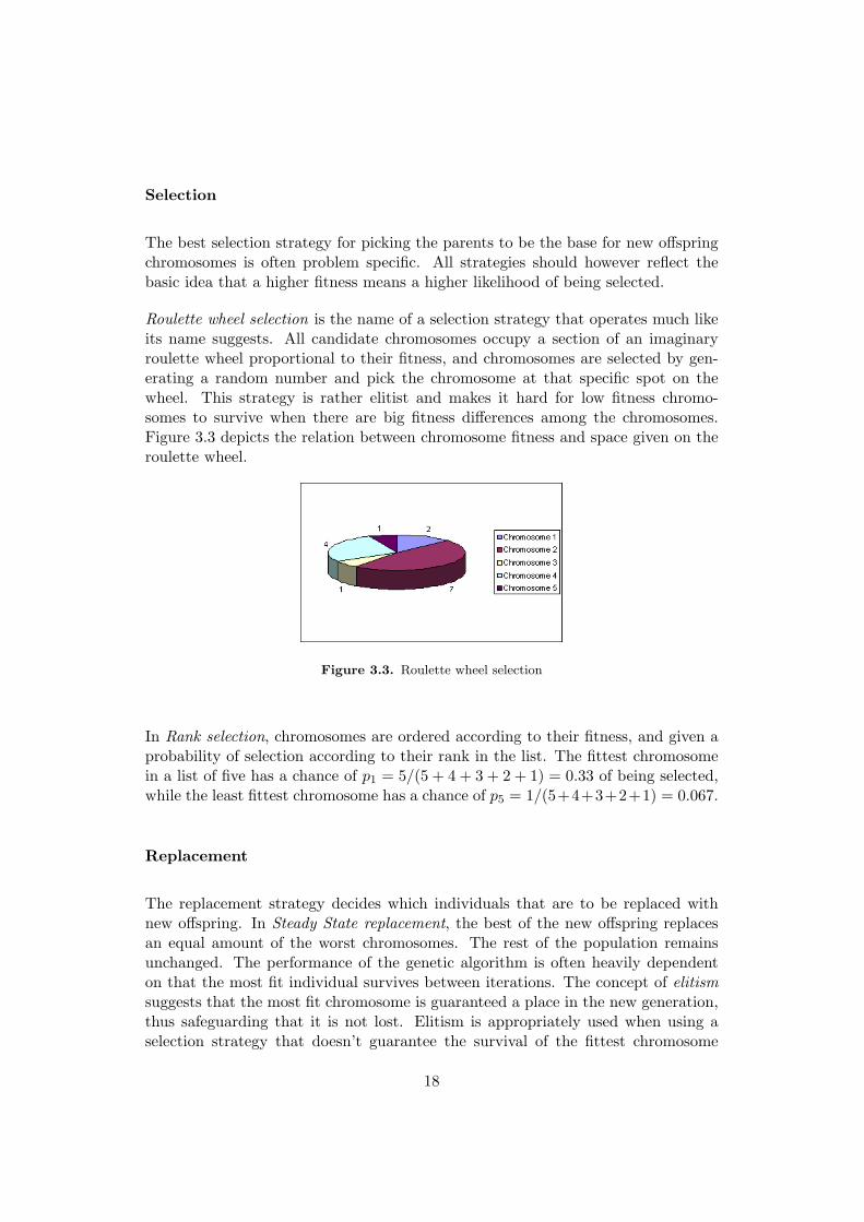
Roulette wheel selection is the name of a selection strategy that operates much likeits name suggests. All candidate chromosomes occupy a section of an imaginaryroulette wheel proportional to their fitness, and chromosomes are selected by gen-erating a random number and pick the chromosome at that specific spot on thewheel. This strategy is rather elitist and makes it hard for low fitness chromo-somes to survive when there are big fitness differences among the chromosomes.Figure 3.3 depicts the relation between chromosome fitness and space given on theroulette wheel.

Figure 3.3. Roulette wheel selection

In Rank selection, chromosomes are ordered according to their fitness, and given aprobability of selection according to their rank in the list. The fittest chromosomein a list of five has a chance of p1 = 5/(5 + 4 + 3 + 2 + 1) = 0.33 of being selected,while the least fittest chromosome has a chance of p5 = 1/(5+4+3+2+1) = 0.067.

Replacement

The replacement strategy decides which individuals that are to be replaced withnew offspring. In Steady State replacement, the best of the new offspring replacesan equal amount of the worst chromosomes. The rest of the population remainsunchanged. The performance of the genetic algorithm is often heavily dependenton that the most fit individual survives between iterations. The concept of elitismsuggests that the most fit chromosome is guaranteed a place in the new generation,thus safeguarding that it is not lost. Elitism is appropriately used when using aselection strategy that doesn’t guarantee the survival of the fittest chromosome

18

[15]. The CHC Strategy combines the old population with an equal amount of newoffspring, and selects the best individuals to form the new population.

Crossover

When parents have been selected according to the used selection strategy, crossoverare performed on the parents to breed new chromosomes. The aim of the cros-sover procedure is to combine traits from the selected chromosomes to form a newchromosome.

How crossover actually is done depends on the encoding used. Binary encodedchromosomes are usually crossed over by replacing a randomly chosen section ofone chromosome with the corresponding content of the other (One Point Cros-sover). Alternatively, each bit position uses the bit at the corresponding positionof a randomly chosen parent. Binary chromosomes can also be subject to somearithmetic operation to perform crossover.

The performance of GA greatly depends on the ability of the crossover operatorto combine solutions into a solution more probable of being successful than a ran-domly selected solution. Unsuccessful crossover operators give recombinations nobetter than randomly selected solutions. A GA implementation with high mutationrate and no significant crossover can be seen as a parallelized version of SA wheresolutions are independently improved.

Mutation

Mutation is performed to introduce slight variations to allow for the exploration ofstates not generated through crossover. It may help the search escape local minimaand find new areas of interest in the problem hyperspace. Suitable mutation ratesare problem dependent, but are usually low compare to the crossover rate. Mutationis critical to the performance of the genetic algorithm, as the crossover operator byitself requires large populations and is ineffective [7].

3.2.3 Stopping Criteria

Common to most stochastic optimization algorithms, we have no clear way of know-ing when to stop the search and accept the currently best solution as the optimal ornear-optimal solution. In GA, we usually fix the number of generations to evolve,or end when the algorithm lack to make progress, which is defined e.g. in terms ofG number of non-improving generations.

19

3.2.4 Genetic Algoritms and Image Registration

Chalermwat [3] gives a comprehensive overview of what has been done in the fieldof GA-based image registration in his dissertation on high performance automaticimage registration for remote sensing, referring to five different studies conductedbetween 1984 and 1994.

Maslov and Gertner [13] investigates the possibility of a dynamic adaption of themutation pool size related to the rate at which the gradient of the fitness functiondecreases between generations in genetic algorithms. This was found to accelerateconvergence and more speedily escape local minima.

Chalermwat and El-Ghazawi [4] uses GA on wavelet transformed input images toconduct multi-resolution image registration.

3.3 Simulated Annealing

Simulated Annealing (SA) is a search heuristic used to solve optimization problems.It has been proven to statistically deliver a globally optimal solution, and can beapplied to a wide range of problems. Its main strength is the ability to escapelocal minima during the search process. SA has been applied to solve a varietyof optimization problems, the most well-known and successful application perhapsbeing the NP-complete Traveling Salesman Problem. Other areas of use includecircuit design, combinatorial optimization, finance, data analysis and imaging.

3.3.1 Background

The optimization technique known as SA was developed from a Monte Carlo im-portance sampling-technique developed by Metropolis 1953 [10]. Its guiding conceptis a temperature schedule that makes searching more effective, inspired by the waymetals are slowly cooled off to gain a minimum energy crystalline structure. Ineach step of the SA algorithm, the current solution is replaced by a randomly se-lected nearby solution from the search space, which is selected with a probabilityrelated to the score difference between the current and the proposed solution, anda ”temperature” variable T .

SA is a metaheuristic in the sense that many choices regarding the implementa-tion of the algorithm are left to the implementer. The main advantage of SA is itspromise to statistically deliver a globally optimal solution, regardless of discontinu-ities, non-linearities, dimension and randomness in the target function. It is also

20

quite simple and straightforward to implement but however often requires problemspecific tuning to perform at its best. Doing this tuning is considered somewhat ofan art, and will receive our focus later in this report. SA is however not withoutdrawbacks, the most negative feature being its slow convergence towards an optimalfit. Variants of SA have been developed to remedy this problem, however often atthe expense of the global optimum guarantee. Another weakness of SA is that thealgorithm does not know if and when it has found the global minimum, which makesstopping criteria an important performance factor.

3.3.2 Algorithm Description

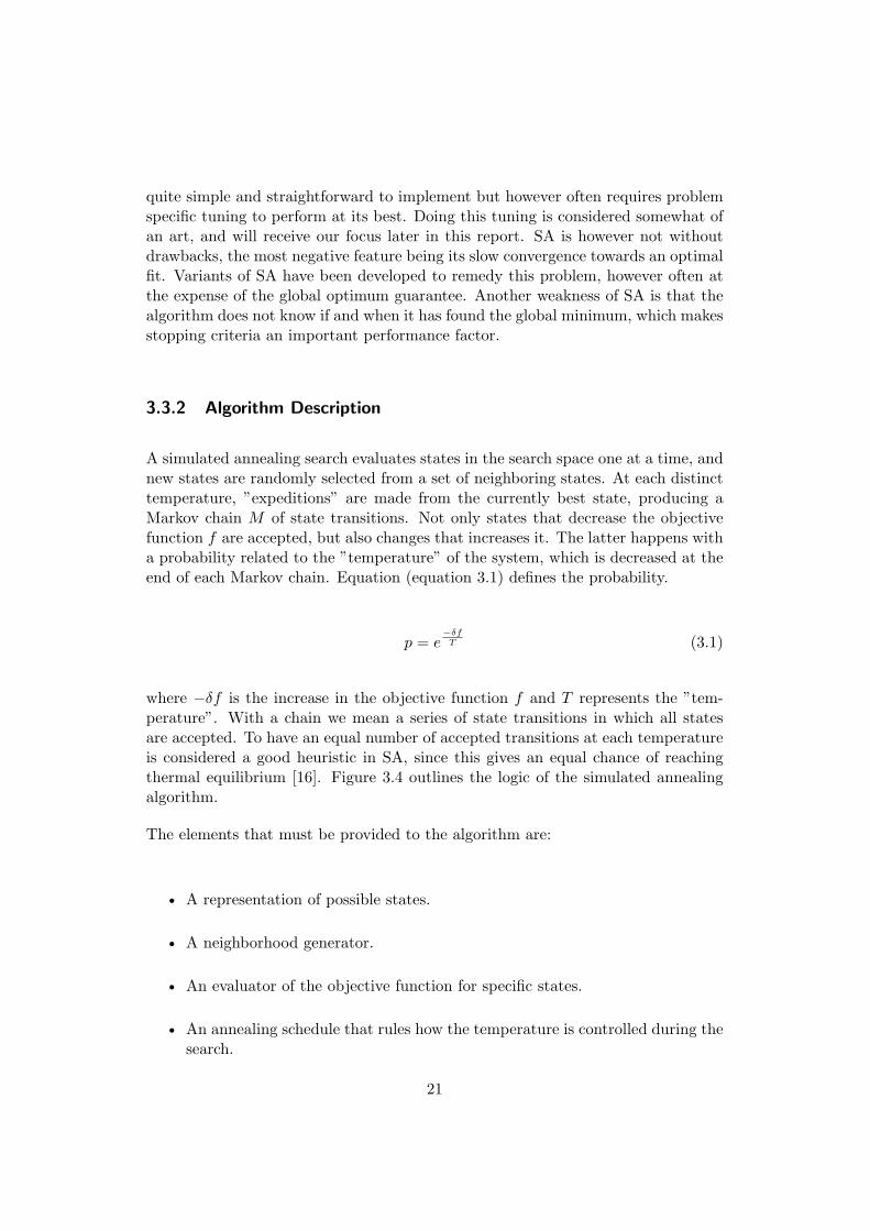
A simulated annealing search evaluates states in the search space one at a time, andnew states are randomly selected from a set of neighboring states. At each distincttemperature, ”expeditions” are made from the currently best state, producing aMarkov chain M of state transitions. Not only states that decrease the objectivefunction f are accepted, but also changes that increases it. The latter happens witha probability related to the ”temperature” of the system, which is decreased at theend of each Markov chain. Equation (equation 3.1) defines the probability.

p = e−δf

T (3.1)

where −δf is the increase in the objective function f and T represents the ”tem-perature”. With a chain we mean a series of state transitions in which all statesare accepted. To have an equal number of accepted transitions at each temperatureis considered a good heuristic in SA, since this gives an equal chance of reachingthermal equilibrium [16]. Figure 3.4 outlines the logic of the simulated annealingalgorithm.

The elements that must be provided to the algorithm are:

• A representation of possible states.

• A neighborhood generator.

• An evaluator of the objective function for specific states.

• An annealing schedule that rules how the temperature is controlled during thesearch.

21

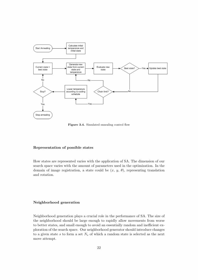
Figure 3.4. Simulated snnealing control flow

Representation of possible states

How states are represented varies with the application of SA. The dimension of oursearch space varies with the amount of parameters used in the optimization. In thedomain of image registration, a state could be (x, y, θ), representing translationand rotation.

Neighborhood generation

Neighborhood generation plays a crucial role in the performance of SA. The size ofthe neighborhood should be large enough to rapidly allow movements from worseto better states, and small enough to avoid an essentially random and inefficient ex-ploration of the search space. Our neighborhood generator should introduce changesto a given state s to form a set Ns of which a random state is selected as the nextmove attempt.

22

State evaluation

State evaluation is simply the process of mapping a distinct scalar value to describethe fitness of a particular state in the search space. In the case of image registration,we use the similarity measure function.

Annealing schedule

The initial temperature T0 is problem specific and depends on the range of valuesthat our objective function f takes. Decreasing of the temperature can be doneeither in an exponential or linear fashion. One of the most common SA variants isBoltzmann Annealing in which the temperature at Markov Chain no. k is definedin equation 3.2.

T (k) =T0

ln k(3.2)

An exponential cooling schedule is a popular alternative, defined in equation 3.3.

Tk+1 = αTk (3.3)

where 0 < α < 1 is the cooling rate. In general, slower cooling rates achieve agreater probability of finding the globally optimal state, but do so at the expenseof computational effort and hence speed.

A stopping criterion for the annealing process needs to be decided on. More orless sophisticated and aggressive strategies can be applied here; common ones in-clude fixing the total number of temperatures or solutions to use or setting a lowertemperature bound.

3.3.3 Simulated Annealing and Image Registration

Quite limited research seems to have been done in the area of applying SA specific-ally to image registration. Luck et al. [12] implemented a hybrid between SimulatedAnnealing and the Iterative Closest Point algorithm, where ICP does most of thework and SA helps finding good starting points and traverse local minima for ICP.The approach proves to be more efficient than the techniques applied individually.

23

Capek [2] studies the performance of several optimization techniques on image regis-tration, finding SA to perform well but unfortunately unable to draw any generalconclusions as many of the configuration parameters were hand selected for theinvestigated problem.

24

Chapter 4

Method

This chapter concerns the method by which the investigation was carried out, anddescribes relevant implementation issues.

4.1 Choice of Method

We begin by stating the requirements of the investigation.

• The system must generate acceptable registration results. This means regis-tration results which by visual inspection seem accurate.

• The system must be fast compared to exhaustive search methods.

• The results of the investigation should if possible be general enough to applyto any SA/GA implementation. If this cannot be motivated, results shouldreflect general SA/GA implementations confined to the image registrationdomain.

The natural choice of method for performing this investigation would be a computersoftware implementation of the algorithms. By constructing test batches, data canbe extracted and analyzed with the aid of some visualization tool. By observingthe search space signature, error rate, convergence and other data, conclusions canbe drawn regarding the performance of particular algorithm configurations.

25

4.2 Conditions and Limitations

Being metaheuristics, the major problem with the genetic algorithm and simulatedannealing is the possibility to extract general results that arguably apply to otheroptimization problems as well. Cost functions with a ”spiky” landscape, filled withlarge variations and local minima are extremely difficult to optimize, and approachesthat function perfectly on more flat landscapes may very well fail here. However,since our concern is image registration, we may assume that the problems givento us have landscapes more or less similar to the one showed in figure 3.1, i.e.landscapes with the global minimum residing significantly deeper than most of themany local minima present. Since it is infeasible to ”optimize the optimization”,we were forced to limit our goals and impose some limitations to the investigation.

With the Genetic Algorithm, we focused on investigating suitable encoding andevolutionary operators. The performance of these should be rather problem inde-pendent, at least within the domain of consumer image registration problems.

With Simulated Annealing, we hoped to extract general results regarding suitableneighborhood generators. Suitable Markov chain lengths and cooling schedules arelikely to hold for problems of similar search space size, but might be sub-optimal indifferently sized problems. A final stitching application should therefore allow forthe Markov chain length to be set manually.

4.3 Experimental Setting

This section describes the setting in which the investigation was made.

4.3.1 Images

Initial tests were performed on a pair of photographs of size 528x359 pixels convertedto grayscale. The photographs were acquired using planar rotation of a CanonDigital IXUS 430 digital camera. The camera was not mounted on a tripod buthand-held, which ought to reflect common consumer usage conditions. Figure 5.1shows the photographs. In addition to these tests, two suites of 6 photographs eachwere stitched and the results evaluated.

26

4.3.2 Preprocessing

Preprocessing included projecting both reference and input images onto a cylindricalsurface. A 5x5 pixel Gaussian blur was applied to reduce noise, after which a3x3 pixel Laplacian kernel was used to find edges. The edge map was used toidentify 32x32 pixel sub-images in the reference image of particular interest duringregistration. Sub-images were computed for a confined area of the rightmost part ofthe reference image, since this is where we expect overlap. The area was chosen tohave upper left corner (blocksX−6, 4) and lower right corner (blocksX, blocksY −4),where blocksX and blocksY denote the total number of sub-image blocks in theimage. 25% of the highest ranked sub-images was used during the registrationprocess. SSD was used as similarity measure.

The result of an exhaustive search on the tested problems served as ground truthfor performance comparisons. The results from each exhaustive search was alsosaved to disk in order to speed up batch runs by allowing O(1) look-up of the costfunction.

4.3.3 State Representation

States were represented as sets of (x, y, θ, s), where x and y denotes the state offsetcoordinate, θ the amount of counter clockwise rotation, and s is the scaling ratio.We argue that these transformations suffice to get good image registration results.This 4D search space should also be vast and complex enough for coincidence tonot play a role in the performance of the algorithm configurations.

The rotation parameter took values in the range [0,maxRot]. To extract the actualrotation degree, the value was adjusted to the range [−maxRot

2 , maxRot2 ] and scaled

with a precision constant rotPrecision. A value of rotPrecision = 10 was used.

The scaling parameter took take values in the range [0,maxScale]. To extract theactual scaling constant, the value was adjusted to the range [−maxScale

2 , maxScale2 ],

scaled with a precision constant scalePrecision and incremented by 1. A value ofscalePrecision = 100 was used.

Bilinear interpolation was used in rotation and scaling.

4.3.4 Sampling

All configurations were sampled a number of times to ensure certain statisticalconfidence on the accuracy of the generalization from the extracted results. The

27

confidence interval for the population1 mean is given by equation 4.1.

I = X ± Zα/2σ√n

(4.1)

where n is the number of samples and σ is the standard deviation of the population.In our case, the population is infinite and σ unknown, why we approximate it withthe standard deviation s of the sample set. The confidence level of the interval isgiven by (1−α). Zα/2 gives the offset on the normal curve for excluding an area α.A common confidence level is 95%, giving Z0.25 = 1.96.

For the purpose of evaluating the average error of a configuration, 30 iterations willbe used. This since the standard deviation of the average error usually is aroundσ = 2. A confidence level of 95% with this population gives X ± 0.24, which seemsas an acceptable level of uncertainty for our purposes.

4.4 Performance Evaluation and Comparison

Results from the best genetic algorithm and simulated annealing configurations werecompared with results from exhaustive registration searches and iterative gradientdescent. Since the similarity measure is the by far most computationally expensiveoperation, we argue that the number of evaluated states in the search space servesas a good measure of time consumption of the tested algorithms and that other al-gorithmic computations should be neglectable. The error of a registration is definedas the registration’s Euclidean distance from the optimal match.

4.5 Genetic Algorithms

The main objective of the tests on the genetic algorithm was to evaluate the perform-ance of different runtime-parameters. Population size, crossover rate and mutationrate were varied to form different configurations that could be evaluated. In additionto this, different encodings, crossover and mutation operators were tested.

1where population refers to the set of possible samples from a given configuration

28

4.5.1 Limitations

Due to the huge amount of available tuning parameters, some parameters were fixedin the investigation.

• Roulette Wheel selection was used in all tests. This is motivated by thefact that it is a commonly used selection scheme that is relatively easy toimplement and understand. The strategy is also appealing due to its closeresemblance with nature’s own selection strategy. Roulette Wheel Selectionis also less CPU intensive than e.g. deterministic selection, and performs atleast equally well [7].

• The most fit individual always survives to the next generation (elitism). Thisenables rather intensive rates of crossover and mutation without risking tolose the currently best found state.

4.5.2 Tested Parameters

Population Size

Tested population sizes were S ∈ {9, 19, 29, 39, 49, 59, 69, 79, 89, 99, 149, 199, 249}.Since crossover is done pair wise, and one individual is pre-selected through elitism,the odd population size makes the implementation more comfortable. Chalermwatrefers to a study where population sizes of 10-160 have proven to be suitable formost problems [3]. To get some indication about the performance on larger sizes,199 and 249 were also included in the test.

Encodings

Tested encodings include the traditional binary chromosome encoding, and a value-based approach where states are stored ”as is” without encoding. In binary encod-ing, each parameter gets a number of bits needed to encode the range of possiblevalues, and all bit parts are appended to form a full chromosome representing astate.

Crossover and Mutation

Crossover and mutation rates are tested in the range [0.0, 1.0] respectively. How theoperators work depend on the encoding used:

29

• Binary encoding crossover 1: Single Point Crossover. A randomly selected bitdivides the genes, and the portions on the least significant side are swappedbetween the genes.

• Binary encoding crossover 2: Two Point Crossover. Two bits are randomlyselected, and the portion in between is swapped between genes.

• Binary encoding mutation: A randomly selected bit is inverted.

• Value encoding crossover 1: y-offsets are switched between genes. θ-part isswitched with probability 0.5.

• Value encoding crossover 2: A random value a in the range [0, 1] determineshow much of each gene that will contribute in the crossover. Offspring are(ax1 + (1− a)x1, ay1 + (1− a)x2, aθ1 + (1− a)θ2) and (ax2 + (1− a)x1, ay2 +(1− a)x2, aθ2 + (1− a)θ1).

• Value encoding mutation 1: x and y offsets are incremented/decremented witha random number in the range [−2, 2]. θ and s are incremented/decrementedwith a random number in the [−1, 1].

• Value encoding mutation 2: Exponential distribution of mutation, large muta-tions are less likely than smaller ones.

We tested six different encoding/operator setups:

• BIN1 - Binary encoding with single point crossover

• BIN2 - Binary encoding with two-point crossover

• VAL11 - Value encoding with crossover 1 and mutation 1.

• VAL12 - Value encoding with crossover 1 and mutation 2.

• VAL21 - Value encoding with crossover 2 and mutation 1.

• VAL22 - Value encoding with crossover 2 and mutation 2.

To better understand the different properties of these encoding/operator setups, aplot was made of the states visited during a test run of each setup. We will call thisplot a search space signature of the setup.

4.5.3 Proposed Enhancements

Finally, we propose a few enhancements to the basic algorithm.

30

Neighborhood Search

A simple strategy that could possibly increase the efficiency of the search is tocalculate the fitness of the closest states in the hyperspace each time a new beststate is found. This is likely to speed up convergence at the end of the search,where genetic algorithms sometimes are slow. This rule could be applied recursively,which would result in something similar to a gradient descent towards an eventuallysurrounding minimum. The neighborhood strategy was realized by increasing anddecreasing each of the four parameters in the search set with integers in the range[-1,1].

Adaptive mutation rate

Instead of a fixed mutation rate during the entire evolutionary process, an adaptivemutation rate that changes in accordance to the current population between gen-erations could possibly improve performance. The wanted behavior of the GA isto avoid getting stuck in local minima, and to rapidly investigate candidate statesfurther away.

A naive but rather computationally inexpensive approach to an adaptive mutationrate is to calculate the standard deviation between states in the hyperspace. Asmall standard deviation indicates focus around a (possibly local) minima point,and could be remedied by a higher mutation rate to introduce new states. A largestandard deviation on the other hand, suggests a lower mutation rate, to concentratethe search around the currently fittest states.

We will treat each search space parameter individually, and compute the final muta-tion rate at each evolution according to equation 4.2

pmutationx = 1− σx/σx0

pmutationy = 1− σy/σy0

pmutationθ= 1− σθ/σθ0

pmutations = 1− σs/σs0

pmutation = (pmutationx + pmutationy + pmutationθ+ pmutations)/4

(4.2)

where σx0 , σy0 , σθ0 , σs0 denotes the standard deviation of the initial population foreach parameter respectively.

31

4.6 Simulated Annealing

The simulated annealing algorithm is evaluated with the purpose of finding suitableruntime-parameters for our image registration implementation. Different coolingrates and Markov chain lengths are tested to find suitable configurations and stop-ping criteria. In addition, some enhancements are suggested and evaluated.

All tests will make use of a temperature schedule with exponential cooling rate α,see equation 3.3. The stopping criterium is based on the acceptance ratio fallingbelow a predefined threshold, pacc < pstop, combined with 1 non-improving chain.

4.6.1 Initial Temperature

Finding a suitable initial temperature is an important factor to the performanceof SA. Since the initial temperature varies between different problem instances, ageneral approach to this is needed. A suitable initial temperature should give aprobability p0 = 0.8 that an increase is accepted [1]. This can be estimated bycalculating the average increase δf in the objective function during an initial searchwhere all increases are accepted. T0 is then given by:

T0 =−δf

ln p0(4.3)

The initial temperature will be more accurate, and the annealing more effective,the more samples that are taken from the search space. Another approach is tocontinuously raise the temperature with a constant factor between chains until theproper acceptance rate is reached. However, due to natural fluctuations in theacceptance rate and the sensitivity to the chain length, this method seems moreuncertain and harder to apply. Hence, we used the former method, which we argueshould sample a small percentage of the entire search space before annealing. Sometrial runs suggested that 0.001 is a suitable factor.

4.6.2 Neighborhood Generation

With a reasonably good temperature schedule, the most important factor to thesuccess of a SA run is the neighborhood generation function. The generation shouldensure that all states in the state space are reachable from any particular state, overa Markov walk. The generating function usually introduces small random changesto the parameters of the current state. How these random changes most suitably

32

are bounded and distributed is subject to trial and error. Equation 4.4 shows acommon neighborhood generation function that was used in the tests.

si+1 = si + rm (4.4)

where si denote the current state, si+1 denotes a neighboring state, r is a uniformlydistributed pseudorandom number in the range [−1, 1], and m is a step vectorregulating the size of the neighborhood.

Temperature Driven Neighborhood

The range of the neighborhood should decrease as the annealing progresses. Astraightforward way of accomplishing this is to make the range dependent with thetemperature. We evaluated a simple approach where the range is given by eachparameter scaled with the ratio of the current to the starting temperature, definedin equation 4.5.

m = [w ∗ g(T ), h ∗ g(T ),maxRot ∗ g(T ),maxScale ∗ g(T )]g(T ) = T

T0

(4.5)

where w defines the width of the search space, h the height of the search space,maxRot the number of available rotations, and maxScale the number of scales. Aproblem with this approach is that the step vector will become zero given enoughtemperature decreases. To resolve this, we simply made sure that any parameternever gets less than 4. The temperature driven neighborhood will be referred to asTMP.

Acceptance Ratio Driven Neighborhood

Corana et al. develops a method in which the neighborhood size is variable withrespect to the acceptance ratio during annealing [6]. The goal is to maintain anacceptance ratio of approximately pacc = 0.5, motivated by the argument that a lowrate is undesirable due to the wasted computational effort associated with rejectedtransitions, and a high rate is undesirable because of slow convergence towards theoptimum. Corana’s method makes use of a function g(pacc) (equation 4.6) to controlthe step vector m.

33

g(pacc) =

1 + cpacc−0.6

0.4 if pacc > 0.6(1 + c0.4−pacc

0.4 )−1 if pacc < 0.41 else

(4.6)

where c controls the size of the neighborhood. Corana recommends c = 2, and thisvalue was used in our tests. The method is interesting since it gives a variable neigh-borhood size which needs no adjustment to specific image registration problems. Itmay also serve to put the performance of the other tested neighborhood generatorsin perspective. Corana’s method will be referred to as COR.

Miki et al. proposes some modifications to Corana’s Method, claiming that a goalacceptance ratio of pacc = 0.5 is weakly motivated and that the fixed magnificationconstant c is problem dependent [14]. They propose a new method called AdvancedAdaptive Neighborhood (AAN) which allows for any target acceptance rate to beselected, and a recursively defined magnification factor which adapts during theannealing process. Equation 4.7 outlines the method. We tested the AAN methodwith p1 = 0.3 and p2 = 0.6.

g(pacc) =

H0(pacc if pacc > p1

0.5 if pacc < p2

1 else(4.7)

where p1 and p2 defines the upper and lower bounds of the goal acceptance rate.

H0 = H0 ∗H1 H0 is initially set to 2.0 (4.8)

H1 =

2.0 if pacc > p1

0.5 if pacc < p2

1 else(4.9)

Fixed Neighborhood

In addition to the variable neighborhoods, we test a fixed neighborhood size, settingm = [16, 16, 16, 16]. This fixed neighborhood generator will be referred to as FIX16.

34

4.6.3 Cooling Rates and Chain Lengths

Exponential cooling rates are tested with α = {0.97, 0.95, 0.90, 0.85, 0.80, 0.75, 0.70}.α ∈ [0.80, 0.99] is widely as accepted as suitable. 0.75 and 0.70 was included in thetest as well to evaluate rapid cooling.

Tested fixed-length Markov chains length are M = {5, 10, 20, 30, 40, 50, 75, 100}.

4.6.4 Stopping Criteria

Busetti [1] suggests that no improvement during an entire Markov Chain combinedwith the acceptance ratio falling below a given small value pstop should serve asan indication of lacking progress. The acceptance ratio pacc is defined as the ratioof accepted to attempted transitions during a complete chain. Tested acceptanceratios are: pacc = {0.10, 0.05, 0.01}.

4.6.5 Proposed Enhancement

We applied the neighborhood search proposed for the genetic algorithm to thesimulated annealing as well.

4.7 Implementation

This section describes implementation specific details.

4.7.1 Environment

Experiments were conducted with a Visual Studio .NET 2003 C++ implementationof the given algorithms, on a 1 GHz Pentium IIIM Laptop PC running WindowsXP SP2. Results were graphically visualized using MATLAB 6.2 for Windows.

4.7.2 Program Structure

The program was structured in an object-oriented way. The table below brieflydescribes essential component classes of the implementation.

35

Component DescriptionApplication The main thread, interacts with the Révolte platform.

Image Routines for manipulation of images.Similarity Routines for calculating similarity measures.

GA Routines for genetic algorithm runs.SA Routines for simulated annealing.

Table 4.1. Program Components

4.7.3 Other Issues

A cache table of evaluated similarity measures was maintained to provide fast lookupfor already seen solution states. Batch runs made use of a static cache that main-tained its data in between test iterations. Each separate run has a separate tableto monitor the amount of revisits to already seen states.

Random number generation was done with a C/C++ implementation of the pseu-dorandom Mersenne Twister2.

2MoreinformationontheMersenneTwistercanbefoundonitshomepage,http://www.math.sci.hiroshima-u.ac.jp/~m-mat/MT/emt.html

36

Chapter 5

Experimental Results

In this chapter we evaluate results from the investigation method described in theprevious chapter. We end with a few comparisons with other optimization tech-niques.

5.1 Basic Implementation

This section shows the result of a sample image registration task solved with ex-haustive search. The approach is based on a full search of the SSD function on abinary edge map of a smoothed version of the original images. The smoothing filterused is a 3x3 averaging filter mask. Images were captured with camera1 rotationsand projected on a cylindrical surface ( π

12 rad per image) prior to registration. Noconsiderations of lens distortion were taken.

Figure 5.1 shows the stitched pictures with a manually selected reference windowmarked on the left and the resultant matching window after the registration pro-cedure marked on the right.

The images were merged using linear distribution of median intensity differences,with a neighborhood of 10 pixels and the median based on ±3 pixels around a givenrow. The alignment process took about 4 minutes to perform on a Pentium IIIMobile 1 GHz CPU using a C++ implementation.

1a Canon Digital IXUS 400, 4 megapixel

37

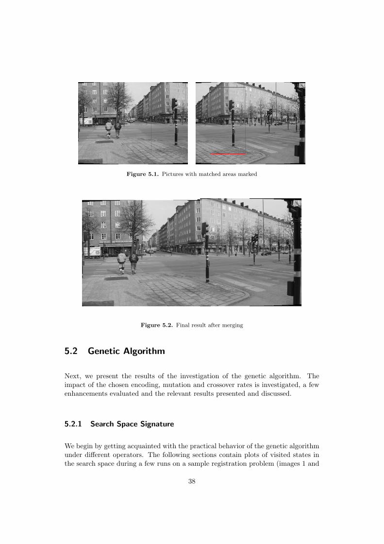
Figure 5.1. Pictures with matched areas marked

Figure 5.2. Final result after merging

5.2 Genetic Algorithm

Next, we present the results of the investigation of the genetic algorithm. Theimpact of the chosen encoding, mutation and crossover rates is investigated, a fewenhancements evaluated and the relevant results presented and discussed.

5.2.1 Search Space Signature

We begin by getting acquainted with the practical behavior of the genetic algorithmunder different operators. The following sections contain plots of visited states inthe search space during a few runs on a sample registration problem (images 1 and

38

2). The rotation and scaling parameters have been omitted from the plots to makethem more easily interpretable2.

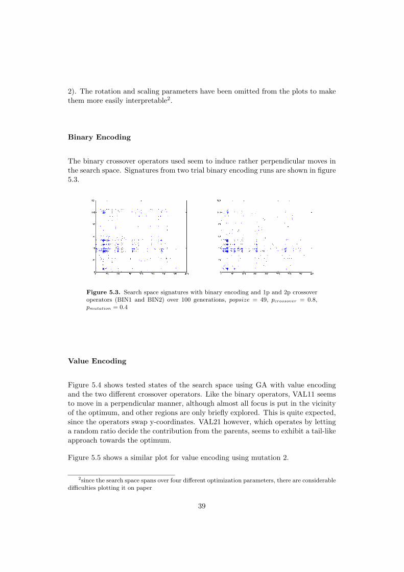
Binary Encoding

The binary crossover operators used seem to induce rather perpendicular moves inthe search space. Signatures from two trial binary encoding runs are shown in figure5.3.

Figure 5.3. Search space signatures with binary encoding and 1p and 2p crossoveroperators (BIN1 and BIN2) over 100 generations, popsize = 49, pcrossover = 0.8,pmutation = 0.4

Value Encoding

Figure 5.4 shows tested states of the search space using GA with value encodingand the two different crossover operators. Like the binary operators, VAL11 seemsto move in a perpendicular manner, although almost all focus is put in the vicinityof the optimum, and other regions are only briefly explored. This is quite expected,since the operators swap y-coordinates. VAL21 however, which operates by lettinga random ratio decide the contribution from the parents, seems to exhibit a tail-likeapproach towards the optimum.

Figure 5.5 shows a similar plot for value encoding using mutation 2.

2since the search space spans over four different optimization parameters, there are considerabledifficulties plotting it on paper

39

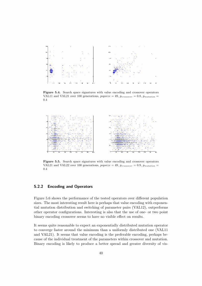
Figure 5.4. Search space signatures with value encoding and crossover operatorsVAL11 and VAL21 over 100 generations, popsize = 49, pcrossover = 0.8, pmutation =0.4

Figure 5.5. Search space signatures with value encoding and crossover operatorsVAL21 and VAL22 over 100 generations, popsize = 49, pcrossover = 0.9, pmutation =0.4

5.2.2 Encoding and Operators

Figure 5.6 shows the performance of the tested operators over different populationsizes. The most interesting result here is perhaps that value encoding with exponen-tial mutation distribution and switching of parameter pairs (VAL12), outperformsother operator configurations. Interesting is also that the use of one- or two pointbinary encoding crossover seems to have no visible effect on results.

It seems quite reasonable to expect an exponentially distributed mutation operatorto converge faster around the minimum than a uniformly distributed one (VAL11and VAL21). It seems that value encoding is the preferable encoding, perhaps be-cause of the individual treatment of the parameters within crossover and mutation.Binary encoding is likely to produce a better spread and greater diversity of vis-

40

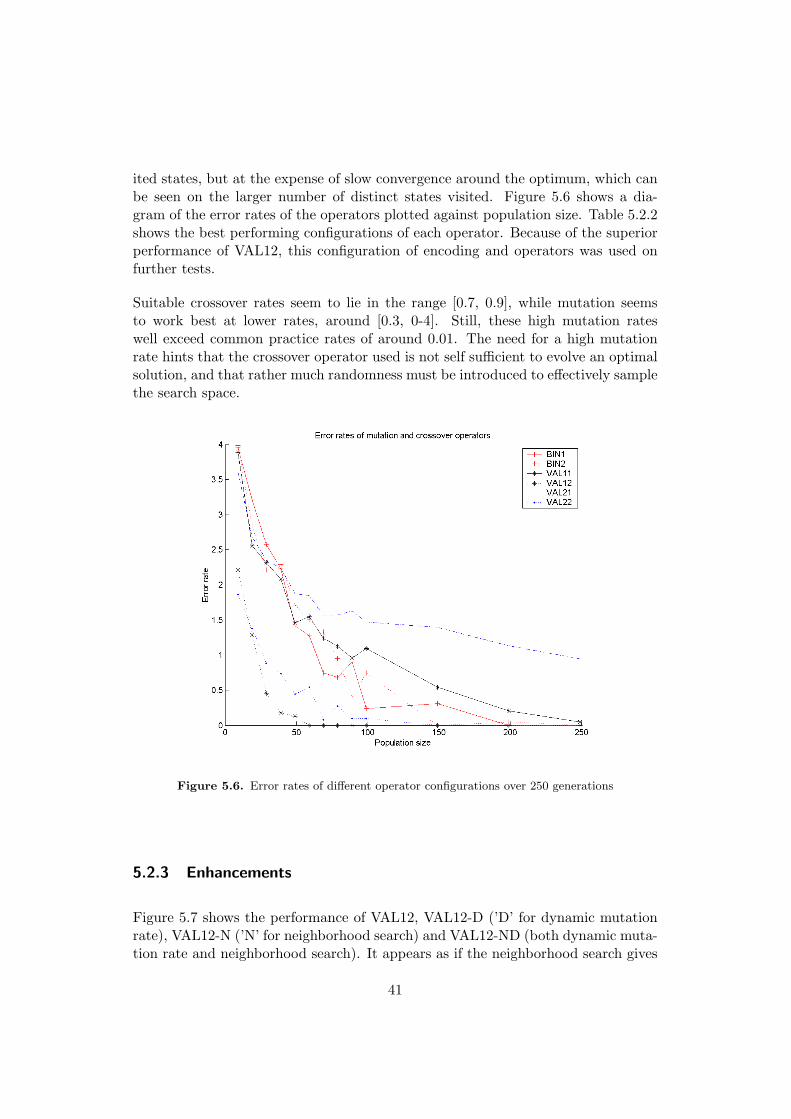
ited states, but at the expense of slow convergence around the optimum, which canbe seen on the larger number of distinct states visited. Figure 5.6 shows a dia-gram of the error rates of the operators plotted against population size. Table 5.2.2shows the best performing configurations of each operator. Because of the superiorperformance of VAL12, this configuration of encoding and operators was used onfurther tests.

Suitable crossover rates seem to lie in the range [0.7, 0.9], while mutation seemsto work best at lower rates, around [0.3, 0-4]. Still, these high mutation rateswell exceed common practice rates of around 0.01. The need for a high mutationrate hints that the crossover operator used is not self sufficient to evolve an optimalsolution, and that rather much randomness must be introduced to effectively samplethe search space.

Figure 5.6. Error rates of different operator configurations over 250 generations

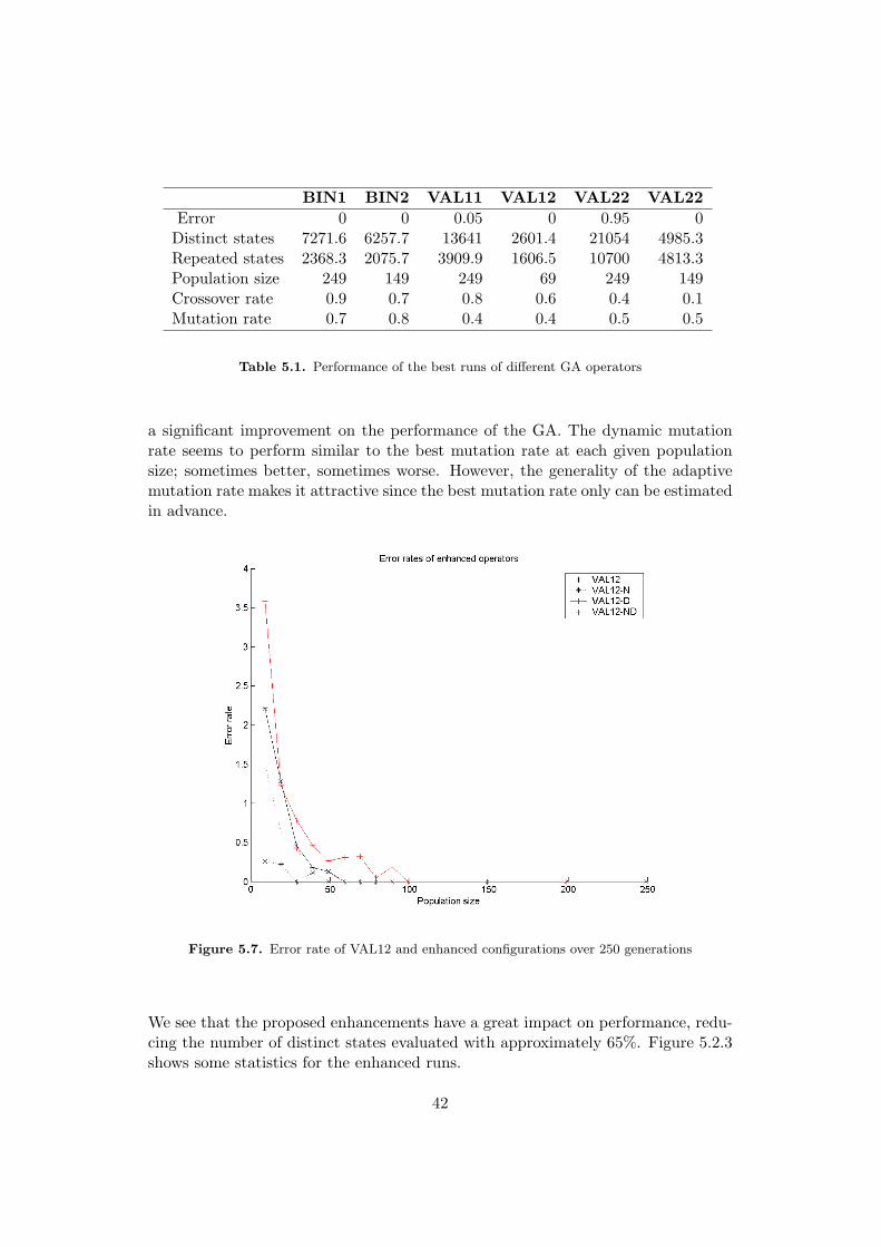
5.2.3 Enhancements

Figure 5.7 shows the performance of VAL12, VAL12-D (’D’ for dynamic mutationrate), VAL12-N (’N’ for neighborhood search) and VAL12-ND (both dynamic muta-tion rate and neighborhood search). It appears as if the neighborhood search gives

41

BIN1 BIN2 VAL11 VAL12 VAL22 VAL22Error 0 0 0.05 0 0.95 0

Distinct states 7271.6 6257.7 13641 2601.4 21054 4985.3Repeated states 2368.3 2075.7 3909.9 1606.5 10700 4813.3Population size 249 149 249 69 249 149Crossover rate 0.9 0.7 0.8 0.6 0.4 0.1Mutation rate 0.7 0.8 0.4 0.4 0.5 0.5

Table 5.1. Performance of the best runs of different GA operators

a significant improvement on the performance of the GA. The dynamic mutationrate seems to perform similar to the best mutation rate at each given populationsize; sometimes better, sometimes worse. However, the generality of the adaptivemutation rate makes it attractive since the best mutation rate only can be estimatedin advance.

Figure 5.7. Error rate of VAL12 and enhanced configurations over 250 generations

We see that the proposed enhancements have a great impact on performance, redu-cing the number of distinct states evaluated with approximately 65%. Figure 5.2.3shows some statistics for the enhanced runs.

42

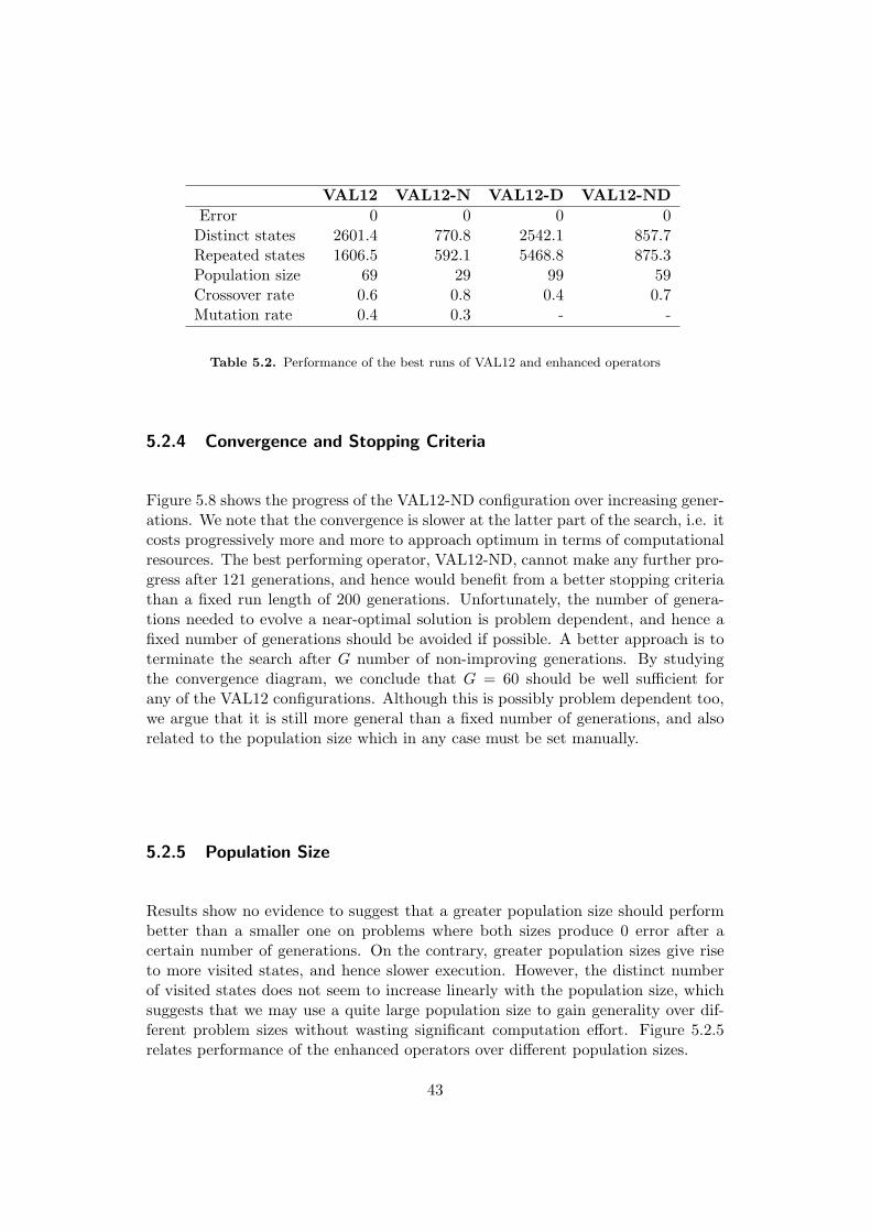
VAL12 VAL12-N VAL12-D VAL12-NDError 0 0 0 0

Distinct states 2601.4 770.8 2542.1 857.7Repeated states 1606.5 592.1 5468.8 875.3Population size 69 29 99 59Crossover rate 0.6 0.8 0.4 0.7Mutation rate 0.4 0.3 - -

Table 5.2. Performance of the best runs of VAL12 and enhanced operators

5.2.4 Convergence and Stopping Criteria

Figure 5.8 shows the progress of the VAL12-ND configuration over increasing gener-ations. We note that the convergence is slower at the latter part of the search, i.e. itcosts progressively more and more to approach optimum in terms of computationalresources. The best performing operator, VAL12-ND, cannot make any further pro-gress after 121 generations, and hence would benefit from a better stopping criteriathan a fixed run length of 200 generations. Unfortunately, the number of genera-tions needed to evolve a near-optimal solution is problem dependent, and hence afixed number of generations should be avoided if possible. A better approach is toterminate the search after G number of non-improving generations. By studyingthe convergence diagram, we conclude that G = 60 should be well sufficient forany of the VAL12 configurations. Although this is possibly problem dependent too,we argue that it is still more general than a fixed number of generations, and alsorelated to the population size which in any case must be set manually.

5.2.5 Population Size

Results show no evidence to suggest that a greater population size should performbetter than a smaller one on problems where both sizes produce 0 error after acertain number of generations. On the contrary, greater population sizes give riseto more visited states, and hence slower execution. However, the distinct numberof visited states does not seem to increase linearly with the population size, whichsuggests that we may use a quite large population size to gain generality over dif-ferent problem sizes without wasting significant computation effort. Figure 5.2.5relates performance of the enhanced operators over different population sizes.

43

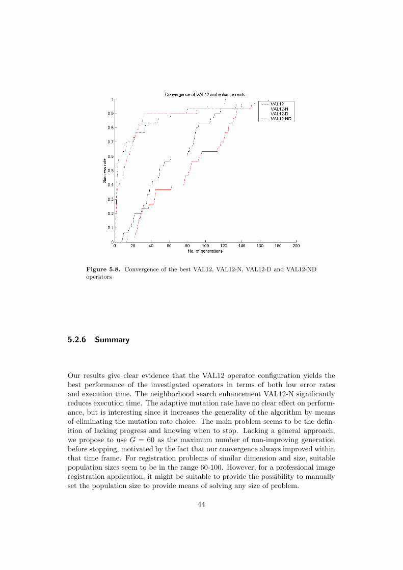
Figure 5.8. Convergence of the best VAL12, VAL12-N, VAL12-D and VAL12-NDoperators

5.2.6 Summary

Our results give clear evidence that the VAL12 operator configuration yields thebest performance of the investigated operators in terms of both low error ratesand execution time. The neighborhood search enhancement VAL12-N significantlyreduces execution time. The adaptive mutation rate have no clear effect on perform-ance, but is interesting since it increases the generality of the algorithm by meansof eliminating the mutation rate choice. The main problem seems to be the defin-ition of lacking progress and knowing when to stop. Lacking a general approach,we propose to use G = 60 as the maximum number of non-improving generationbefore stopping, motivated by the fact that our convergence always improved withinthat time frame. For registration problems of similar dimension and size, suitablepopulation sizes seem to be in the range 60-100. However, for a professional imageregistration application, it might be suitable to provide the possibility to manuallyset the population size to provide means of solving any size of problem.

44

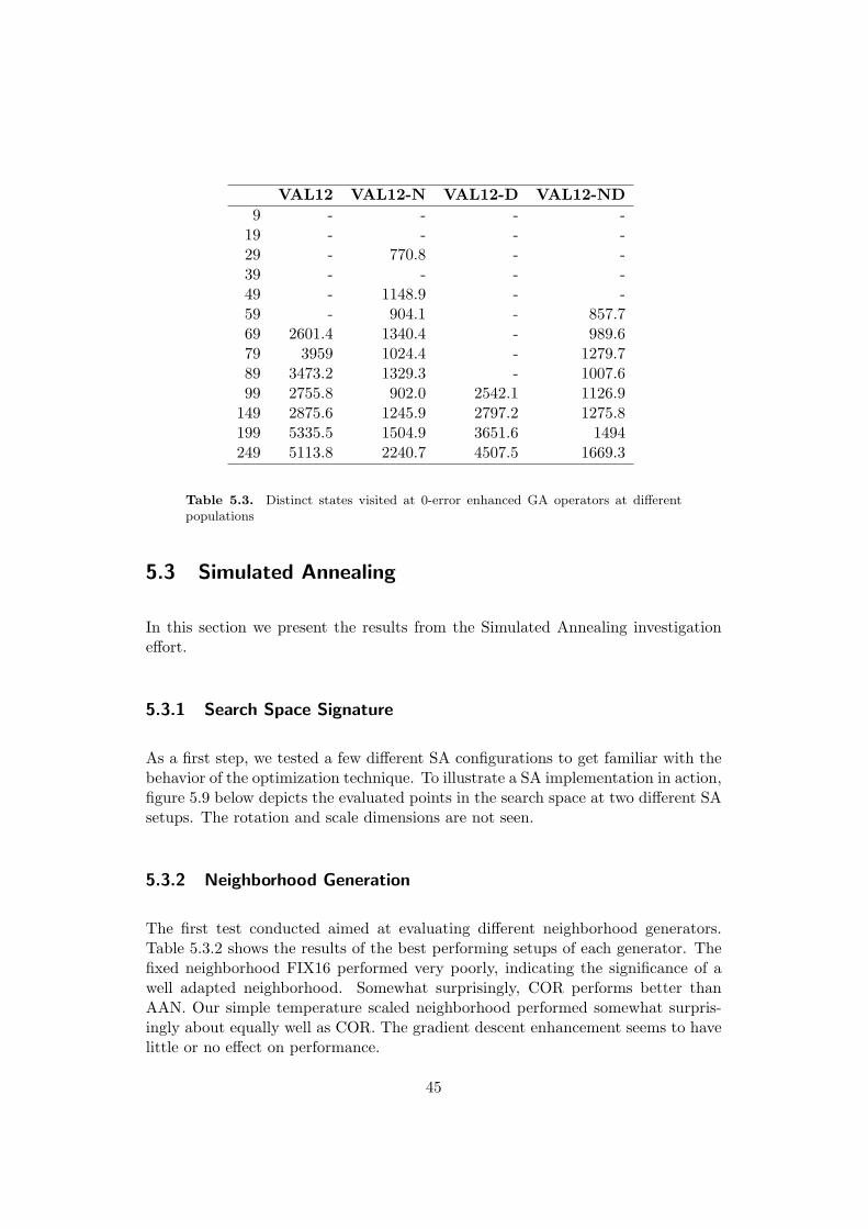
VAL12 VAL12-N VAL12-D VAL12-ND9 - - - -

19 - - - -29 - 770.8 - -39 - - - -49 - 1148.9 - -59 - 904.1 - 857.769 2601.4 1340.4 - 989.679 3959 1024.4 - 1279.789 3473.2 1329.3 - 1007.699 2755.8 902.0 2542.1 1126.9

149 2875.6 1245.9 2797.2 1275.8199 5335.5 1504.9 3651.6 1494249 5113.8 2240.7 4507.5 1669.3

Table 5.3. Distinct states visited at 0-error enhanced GA operators at differentpopulations

5.3 Simulated Annealing

In this section we present the results from the Simulated Annealing investigationeffort.

5.3.1 Search Space Signature

As a first step, we tested a few different SA configurations to get familiar with thebehavior of the optimization technique. To illustrate a SA implementation in action,figure 5.9 below depicts the evaluated points in the search space at two different SAsetups. The rotation and scale dimensions are not seen.

5.3.2 Neighborhood Generation

The first test conducted aimed at evaluating different neighborhood generators.Table 5.3.2 shows the results of the best performing setups of each generator. Thefixed neighborhood FIX16 performed very poorly, indicating the significance of awell adapted neighborhood. Somewhat surprisingly, COR performs better thanAAN. Our simple temperature scaled neighborhood performed somewhat surpris-ingly about equally well as COR. The gradient descent enhancement seems to havelittle or no effect on performance.

45

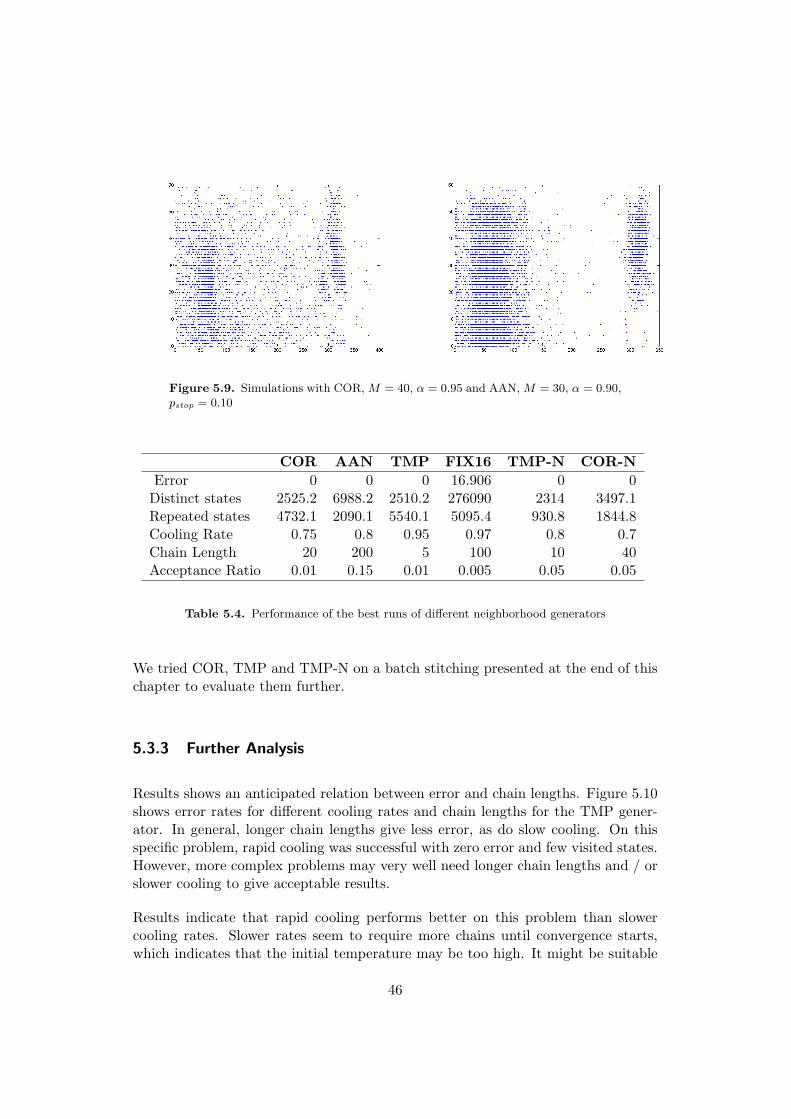
Figure 5.9. Simulations with COR, M = 40, α = 0.95 and AAN, M = 30, α = 0.90,pstop = 0.10

COR AAN TMP FIX16 TMP-N COR-NError 0 0 0 16.906 0 0

Distinct states 2525.2 6988.2 2510.2 276090 2314 3497.1Repeated states 4732.1 2090.1 5540.1 5095.4 930.8 1844.8Cooling Rate 0.75 0.8 0.95 0.97 0.8 0.7Chain Length 20 200 5 100 10 40Acceptance Ratio 0.01 0.15 0.01 0.005 0.05 0.05

Table 5.4. Performance of the best runs of different neighborhood generators

We tried COR, TMP and TMP-N on a batch stitching presented at the end of thischapter to evaluate them further.

5.3.3 Further Analysis

Results shows an anticipated relation between error and chain lengths. Figure 5.10shows error rates for different cooling rates and chain lengths for the TMP gener-ator. In general, longer chain lengths give less error, as do slow cooling. On thisspecific problem, rapid cooling was successful with zero error and few visited states.However, more complex problems may very well need longer chain lengths and / orslower cooling to give acceptable results.

Results indicate that rapid cooling performs better on this problem than slowercooling rates. Slower rates seem to require more chains until convergence starts,which indicates that the initial temperature may be too high. It might be suitable

46

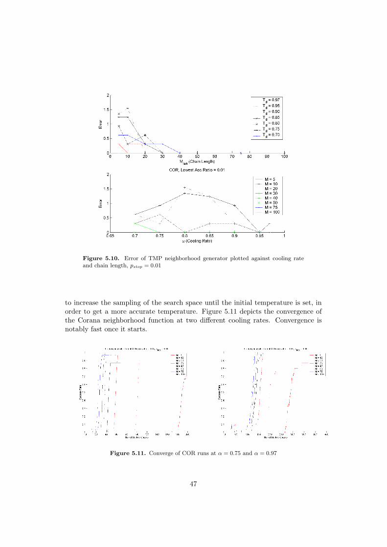
Figure 5.10. Error of TMP neighborhood generator plotted against cooling rateand chain length, pstop = 0.01

to increase the sampling of the search space until the initial temperature is set, inorder to get a more accurate temperature. Figure 5.11 depicts the convergence ofthe Corana neighborhood function at two different cooling rates. Convergence isnotably fast once it starts.

Figure 5.11. Converge of COR runs at α = 0.75 and α = 0.97

47

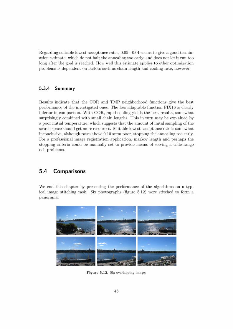
Regarding suitable lowest acceptance rates, 0.05 - 0.01 seems to give a good termin-ation estimate, which do not halt the annealing too early, and does not let it run toolong after the goal is reached. How well this estimate applies to other optimizationproblems is dependent on factors such as chain length and cooling rate, however.

5.3.4 Summary

Results indicate that the COR and TMP neighborhood functions give the bestperformance of the investigated ones. The less adaptable function FIX16 is clearlyinferior in comparison. With COR, rapid cooling yields the best results, somewhatsurprisingly combined with small chain lengths. This in turn may be explained bya poor initial temperature, which suggests that the amount of inital sampling of thesearch space should get more resources. Suitable lowest acceptance rate is somewhatinconclusive, although rates above 0.10 seem poor, stopping the annealing too early.For a professional image registration application, markov length and perhaps thestopping criteria could be manually set to provide means of solving a wide rangeoch problems.

5.4 Comparisons

We end this chapter by presenting the performance of the algorithms on a typ-ical image stitching task. Six photographs (figure 5.12) were stitched to form apanorama.

Figure 5.12. Six overlapping images

48

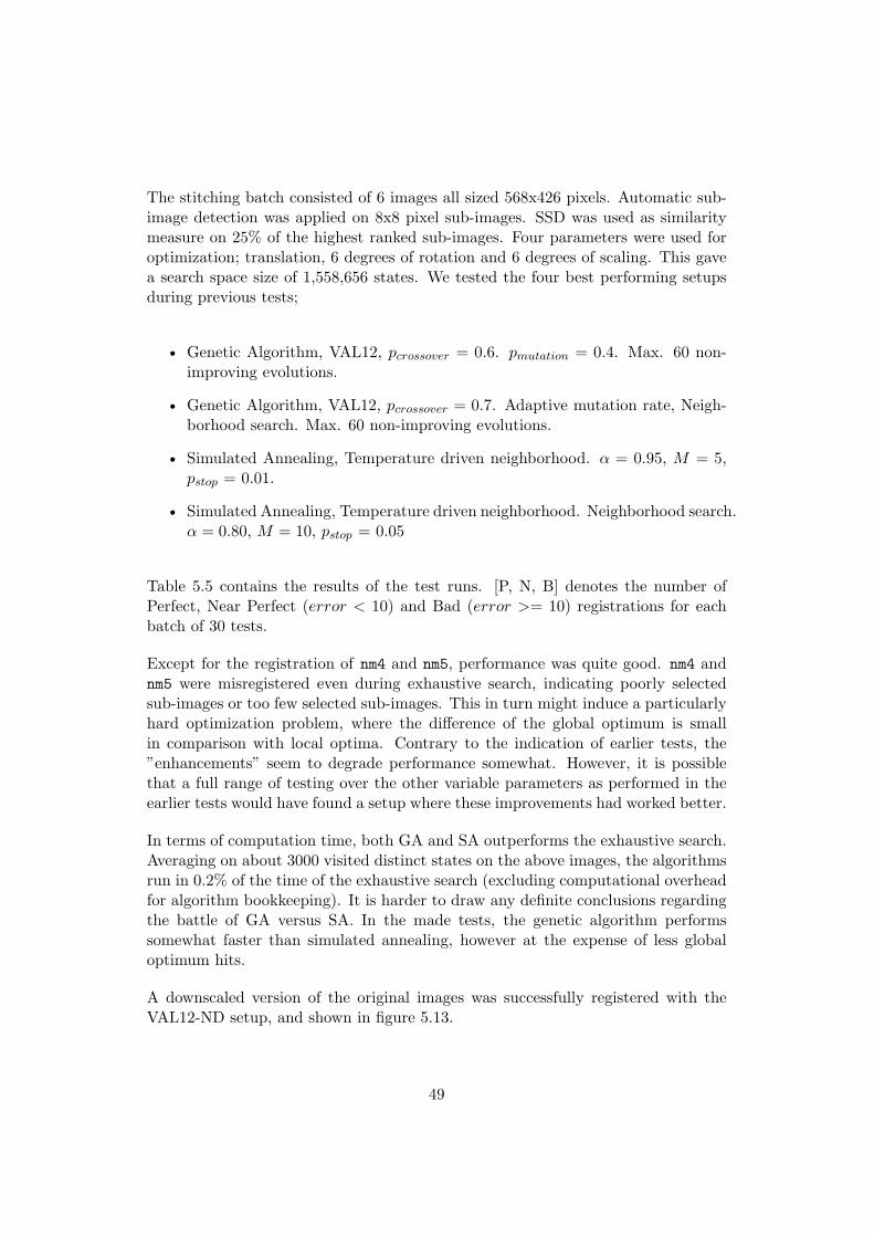
The stitching batch consisted of 6 images all sized 568x426 pixels. Automatic sub-image detection was applied on 8x8 pixel sub-images. SSD was used as similaritymeasure on 25% of the highest ranked sub-images. Four parameters were used foroptimization; translation, 6 degrees of rotation and 6 degrees of scaling. This gavea search space size of 1,558,656 states. We tested the four best performing setupsduring previous tests;

• Genetic Algorithm, VAL12, pcrossover = 0.6. pmutation = 0.4. Max. 60 non-improving evolutions.

• Genetic Algorithm, VAL12, pcrossover = 0.7. Adaptive mutation rate, Neigh-borhood search. Max. 60 non-improving evolutions.

• Simulated Annealing, Temperature driven neighborhood. α = 0.95, M = 5,pstop = 0.01.

• Simulated Annealing, Temperature driven neighborhood. Neighborhood search.α = 0.80, M = 10, pstop = 0.05

Table 5.5 contains the results of the test runs. [P, N, B] denotes the number ofPerfect, Near Perfect (error < 10) and Bad (error >= 10) registrations for eachbatch of 30 tests.

Except for the registration of nm4 and nm5, performance was quite good. nm4 andnm5 were misregistered even during exhaustive search, indicating poorly selectedsub-images or too few selected sub-images. This in turn might induce a particularlyhard optimization problem, where the difference of the global optimum is smallin comparison with local optima. Contrary to the indication of earlier tests, the”enhancements” seem to degrade performance somewhat. However, it is possiblethat a full range of testing over the other variable parameters as performed in theearlier tests would have found a setup where these improvements had worked better.

In terms of computation time, both GA and SA outperforms the exhaustive search.Averaging on about 3000 visited distinct states on the above images, the algorithmsrun in 0.2% of the time of the exhaustive search (excluding computational overheadfor algorithm bookkeeping). It is harder to draw any definite conclusions regardingthe battle of GA versus SA. In the made tests, the genetic algorithm performssomewhat faster than simulated annealing, however at the expense of less globaloptimum hits.

A downscaled version of the original images was successfully registered with theVAL12-ND setup, and shown in figure 5.13.

49

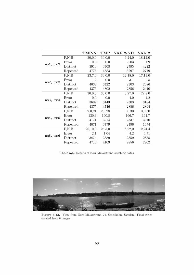
TMP-N TMP VAL12-ND VAL12

nm1, nm2

P,N,B 30,0,0 30,0,0 6,24,0 18,12,0Error 0.0 0.0 5.03 1.9Distinct 3913 3408 2795 4222Repeated 4776 4883 3297 2719

nm2, nm3

P,N,B 23,7,0 30,0,0 12,18,0 17,13,0Error 1.2 0.0 3.1 2.5Distinct 4038 3422 2303 2386Repeated 4375 4802 2856 2440

nm3, nm4

P,N,B 30,0,0 30,0,0 3,27,0 22,8,0Error 0.0 0.0 4.0 1.2Distinct 3602 3143 2303 3184Repeated 4375 4746 2856 2894

nm4, nm5

P,N,B 9,0,21 2,0,28 0,0,30 0,0,30Error 130.3 160.8 166.7 164.7Distinct 4171 3214 2337 3910Repeated 4071 3779 2496 1474

nm5, nm6

P,N,B 20,10,0 25,5,0 8,22,0 2,24,4Error 2.1 1.04 4.2 4.71Distinct 3874 3689 2359 2885Repeated 4710 4109 2856 2902

Table 5.5. Results of Norr Mälarstrand stitching batch

Figure 5.13. View from Norr Mälarstrand 24, Stockholm, Sweden. Final stitchcreated from 6 images.

50

Chapter 6

Conclusions

In this chapter, we briefly review the main results of the thesis. In addition, somesuggestions regarding future work are made.

6.1 Summary

The main conclusion from the extracted results is that both the genetic algorithmand simulated annealing optimization techniques are feasible alternatives to per-forming image registration. Tests performed showed that zero-error registrationswith 4 transformations were repeatedly performed with the time requirements of asmall percentage to exhaustive search. Although a problem with both techniquesis the need for problem specific adjustments of algorithm parameters, we have hadsome general indications, namely:

• Value Encoding combined with crossover by switching parameters betweenoffspring and exponentially distributed mutation is the preferable choice whenimplementing the genetic algorithm to solve an image registration problem.

• The proposed enhancement of neighborhood search after best solution updatesmight speed convergence and give faster execution of the genetic algorithm.

• Adaptive mutation rate lessens the need for problem-specific tuning of geneticalgorithm parameters and may give performance near the best static mutationrate in terms of error and speed.

• Of the compared methods, Corana’s method and temperature variable neigh-borhood generation are the preferable methods of guiding a simulated anneal-ing implementation to solve image registration problems.

51

6.2 Further Work

Given the limited amount of tests performed, further work could be done to furtherinvestigate the use of genetic algorithms and simulated annealing in image regis-tration. Further testing could be done on a wider set of test images reflecting awider set of potential image stitching problems. Implementation of multi-resolutionsearch is likely to increase performance. Both the genetic algorithm and simulatedannealing strategies offer an extensive amount of possible variations to the imple-mentation, and hence there are many ways of further exploring their capabilities.Given the approaches made in this thesis, suitable stopping criteria could be moreextensively researched.

52

Bibliography

[1] Franco Busetti. Simulated annealing overview, 2003.

[2] Martin Capek. Optimisation strategies applied to global similarity based imageregistration methods. URL citeseer.csail.mit.edu/382000.html.

[3] Prachya Chalermwat. High-performance automatic image registration for re-mote sensing. PhD thesis, George Mason University, 1999. ISBN 0-599-52475-8.Director-Tarek El-Ghazawi.

[4] Prachya Chalermwat and Tarek El-Ghazawi. Multi-resolution image regis-traton using genetics. In ICIP99, pages 452–456, 1999. URL citeseer.ist.psu.edu/464186.html.

[5] Chia-Yen Chen and Reinhard Klette. Image stitching - comparisons and newtechniques. In CAIP ’99: Proceedings of the 8th International Conference onComputer Analysis of Images and Patterns, pages 615–622, London, UK, 1999.Springer-Verlag. ISBN 3-540-66366-5.

[6] A. Corana, M., C. Martini, and S. Ridella. Corrigenda: Minimizing multimodalfunctions of continuous variables with the simulated annealing algorithm. ACMTrans. Math. Softw., 15(3):287, 1989. ISSN 0098-3500.

[7] Candida Ferreira. Gene Expression Programming: Mathematical Modeling byan Artificial Intelligence. Gepsoft, 2002. ISBN 972-95890-5-4. URL http://www.gene-expression-programming.com/gep/Books/index.asp.

[8] Duke Gledhill, Gui Yun Tian, David Taylor, and David Clarke. Panoramicimaging - a review. Computers & Graphics, 27(3):435–445, 2003.

[9] Rafael C. Gonzalez and Richard E. Woods. Digital Image Processing. Addison-Wesley Longman Publishing Co., Inc., Boston, MA, USA, 2001. ISBN0201180758.

[10] L. Ingber. Simulated annealing: Practice versus theory. Mathl. Comput. Model-ling, 18(11):29–57, 1993. URL citeseer.ist.psu.edu/ingber93simulated.html.

53

[11] A. Levin, A. Zomet, S. Peleg, and Y. Weiss. Seamless image stitching in thegradient domain, 2003. URL citeseer.csail.mit.edu/663185.html.

[12] J. Luck and L. Hoff. Registration of range data using a hybrid simulatedannealing and iterative closest point algorithm, 2000. URL citeseer.csail.mit.edu/luck00registration.html.

[13] Igor V. Maslov and Izidor Gertner. Gradient-based genetic algorithms in imageregistration. URL citeseer.ist.psu.edu/maslov01gradientbased.html.

[14] Mitsunori Miki, Tomoyuki Hiroyasu, and Keiko Ono. Simulated annealingwith advanced adaptive neighborhood. In Second international workshop onIntelligent systems design and application, pages 113–118, Atlanta, GA, USA,2002. Dynamic Publishers, Inc. ISBN 0-9640398-0-X.

[15] Marek Obitko. Introduction to genetic algorithms, 1998. URL http://cs.felk.cvut.cz/~xobitko/ga/.

[16] Eric Poupaert and Yves Deville. Acceptance driven local search and evolution-ary algorithms. In Lee Spector, Erik D. Goodman, Annie Wu, W. B. Lang-don, Hans-Michael Voigt, Mitsuo Gen, Sandip Sen, Marco Dorigo, ShahramPezeshk, Max H. Garzon, and Edmund Burke, editors, Proceedings of the Ge-netic and Evolutionary Computation Conference (GECCO-2001), pages 1173–1180, San Francisco, California, USA, 7-11 2001. Morgan Kaufmann. ISBN1-55860-774-9. URL citeseer.ist.psu.edu/561109.html.

[17] Richard Szeliski. Image alignment and stitching: A tutorial. Technical report,Microsoft Research, 2004.

54

TRITA-CSC-E 2006:030 ISRN-KTH/CSC/E--06/030--SE

ISSN-1653-5715

www.kth.se