Image Registration for MRI - MSRIlibrary.msri.org/books/Book46/files/07kostelec.pdf · Image Registration for MRI ... a circular feature in the ﬁrst slice appears ... Do we assume

Modern Signal ProcessingMSRI PublicationsVolume 46, 2003

Image Registration for MRI

PETER J. KOSTELEC AND SENTHIL PERIASWAMY

Abstract. To register two images means to align them so that commonfeatures overlap and differences — for example, a tumor that has grown—are readily apparent. Being able to easily spot differences between twoimages is obviously very important in applications. This paper is an intro-duction to image registration as applied to medical imaging. We first defineimage registration, breaking the problem down into its constituent compo-nent. We then discuss various techniques, reflecting different choices thatcan be made in developing an image registration technique. We concludewith a brief discussion.

1. Introduction

1.1. Background. To register two images means to align them, so that com-mon features overlap and differences, should there be any, between the two areemphasized and readily visible to the naked eye. We refer to the process ofaligning two images as image registration.

There are a host of clinical applications requiring image registration. Forexample, one would like to compare two Computed Tomography (CT) scansof a patient, taken say six months ago and yesterday, and identify differencesbetween the two, e.g., the growth of a tumor during the intervening six months(Figure 1). One could also want to align Positron Emission Tomography (PET)data to an MR image, so as to help identify the anatomic location of certainmental activation [43]. And one may want to register lung surfaces in chestComputed Tomography (CT) scans for lung cancer screening [7]. While allof these identifications can be done in the radiologist’s head, the possibilityalways exists that small, but critical, features could be missed. Also, beyondidentification itself, the extent of alignment required could provide importantquantitative information, e.g., how much a tumor’s volume has changed.

Kostelec’s work is supported in part by NSF BCS Award 9978116, AFOSR under awardF49620-00-1-0280, and NIH grants PO1 CA80139. Periaswamy’s work is supported in partby NSF Grants EIA-98-02068 and IIS-99-83806.

161

162 PETER J. KOSTELEC AND SENTHIL PERIASWAMY

Figure 1. Two CT images showing a pelvic tumor’s growth over time. The

grayscale has been adjusted so as to make the tumor, the darker gray area within

the mass in the center of each image, more readily visible. In actuality, it is

barely darker than the background tissue.

When registering images, we are determining a geometric transformationwhich aligns one image to fit another. For a number of reasons, simple im-age subtraction does not work. MR image volumes are acquired one slice at atime. When comparing a six month old MR volume with one acquired yesterday,chances are that the slices (or “imaging planes”) from the two volumes are notparallel. As a result, the perspectives would be different. By this, we mean thefollowing. Consider a right cylindrical cone. A plane slicing through the cone,parallel to its base, forms a circle. If the slice is slightly off parallel, an ellipseresults. In terms of human anatomy, a circular feature in the first slice appearsas an ellipse in the second. In the case of mammography, tissue is compresseddifferently from one exam to the next. Other architectural distortions are possi-ble. Since the body is an elastic structure, how it is oriented in gravity induces avariety of non-rigid deformations. These are just some of the reasons why simpleimage subtraction does not work.

For the neuroscientist doing research in functional Magnetic Resonance Imag-ing (fMRI), the ability to accurately align image volumes is of vital importance.Their results acutely depend on accurate registration. To provide a brief back-ground, to “do” fMRI means to attempt to determine which parts of the brainare active in response to some given stimulus. For instance, the human subject,in the MR scanner, would be asked to perform some task, e.g., finger-tap atregular intervals, or attend to a particular instrument while listening to a pieceof music [20], or count the number of occurrences of a particular color whenshown a collection of colored squares [8]. As the subject performs the task, theresearcher effectively takes 3-D MR movies of the subject’s brain. The goal is toidentify those parts of the brain responsible for processing the information the

IMAGE REGISTRATION FOR MRI 163

Figure 2. fMRI. By registering the frames in the MR “movie” and performing

statistical analyses, the researcher can identify the active part(s) of the brain

by finding those pixels whose intensities change most in response to the given

stimulus. The active pixels are usually false-coloured in some fashion, to make

them more obvious, similar to those shown in this figure.

stimulus provides. The researcher’s hope of accomplishing this is based on theBlood Oxygenation Level Dependent (BOLD) hypothesis (see [6]).

The BOLD hypothesis roughly states that the parts of the brain that processinformation, in response to some stimulus, need more oxygen than those partswhich do not. Changes in the blood oxygen level manifest themselves as changesin the strength of the MR signal. This is what the researcher attempts to detectand measure. The challenge lies in the fact that the changes in signal strength arevery small, on the order of only a few percent greater than background noise [5].And to make matters worse, the subject, despite their noblest intentions, cannothelp but move at least ever so slightly during the experiment. So, before usefulanalysis can begin, the signal strength must be maximized.

This is accomplished by task repetition, i.e., having the subjects repeat thetask over and over again. Then all the image volumes are registered within eachsubject. Assuming gaussian noise, adding the registered images will strengthenthe elusive signal. Statistical analyses are done within subject, and then com-bined across all subjects. This is the usual order of events [18].

1.2. What’s inside this paper. This will be a whirlwind, and by no meansexhaustive, tour of image registration for MRI. We will briefly touch upon a fewof the many and varied techniques used to register MR images. Note that thesurvey articles by Brown [11] and Van den Elsen [38] are excellent sources formore in-depth discussion of image registration, the problem and the techniques.Our purpose here, within this paper, is to whet the reader’s appetite, to stimulateher interest in this very important image processing challenge, a challenge whichhas a host of applications, both in medical imaging and beyond.


The paper is organized as follows. We first give some background and estab-lish a theoretical framework that will provide a means of defining the criticalcomponents involved in image registration. This will enable us to identify thoseissues which need to be addressed when performing image registration. This willbe followed by examples of various registration techniques, explained at varyingdepths. The methods presented are not meant to represent any sort of definitivelist. We want to point out to the reader just some of the techniques which exist,so that they can appreciate how difficult the problem of image registration is, aswell as how varied the solutions can be. We close with a brief discussion.

Acknowledgments. We thank Daniel Rockmore and Dennis Healy for invitingus to participate in the MSRI Summer Graduate Program in Modern SignalProcessing, June 2001. We also thank Digger ‘The Boy’ Rockmore for helpfuldiscussions, and for granting us the use of his image in this paper.

2. Theory

Suppose we have two brain MR images, taken of the same subject, but atdifferent times, say, six months ago and yesterday. We need to align the six monthold image, which we will call the source image, with the one acquired yesterday,the target image. (These terms will be used throughout this paper.) A tumorhas been previously identified, and the radiologist would like to determine howmuch the tumor has grown during the six weeks. Instead of trying to “eyeballit,” the two images would enable an quantitative estimate of the growth rate.How do we proceed?

Do we assume that a simple rigid motion will suffice? Determining the correctrotation and translation parameters is, as we will see later, a relatively quickand straightforward process. However, if non-linear deformations have occurredwithin the brain (which, as described in Sec. 1.1, is likely for any number ofreasons), applying a rigid motion model in this situation will not produce anoptimal alignment. So probably some sort of non-rigid or elastic model wouldbe more appropriate.

Are we looking to perform a global alignment, or a local one? That is, willthe same transformation, e.g., affine, rigid body, be applied to the entire image,or should we instead employ a local model of sorts, where different parts of theimage/volume are moved in different, though smoothly connected, ways?

Should the method we use depend on active participation by the radiologist,to help “prime” or “guide” the method so that accurate alignment is achieved?Or do we instead want the technique to be completely automated and free ofhuman intervention?

Wow, that’s a lot of questions we have to think about, and answer, too. Howdo we begin? To tackle the alignment problem, we had first better organize it.


2.1. The four components. The multitude of challenges inherent in perform-ing image registration can be better addressed by distilling the problem into fourdistinctive components [11].

I. The feature space. Before registering two images, we must decide exactly whatit is that will be registered. The type of algorithm developed depends criticallyon the features chosen. And when you think about it, there are alot of featuresfrom which to choose. Will we work with the raw pixel intensities themselves?Or perhaps the edges and contours of the images? If we have volumetric data,perhaps we should use the surface the volume defines, as in a 3-D brain scan?We could have the user identify features common to both images, with the intentto aligning those landmarks. Then again, if we wish to align images of differentmodalities, say MRI with PET, then perhaps statistical properties of the imagesthat would be optimal for our purpose. So you see, the feature space we choosewill really drive the algorithm we develop.

II. The search space. When one says, “I want to align these two images,” whatis one really saying? That is, what is the rigorous form of the sentence? Thetwo images can be considered samples of two (unknown), compact, real-valuedfunctions, f(x), g(x), defined on Rn (where n is 2 or 3). To align the imagesmeans we wish to find a transformation T (x) such that f(x) = g(T (x)) for allx. Fine. So what kind of transformation are we willing to consider? This is theSearch Space we need to define.

For example, you can consider the simple rigid body transformations, rotationplus translation. Or, if you would like to account for differences in scale, you mayinstead decide to search for the best affine transformation. But both of thesetransformations are global in some respect, and you may want to do somethingmore localized or elastic, and transform different parts of the image by differingamounts, e.g., to account for non-uniform deformations. Your decision here willvery much influence the nature of the registration algorithm.

III. The search strategy. Suppose we have chosen our Search Space. We selecta transformation T0(x) and try it. Based on the results of T0(x), how shouldwe choose the next transformation, T1(x), to try? There are any number ofways: Linear Programming techniques; a relaxation method; some sort of energyminimization.

IV. The similarity metric. This ties in with the Search Strategy. When compar-ing the new transformation with the old, we need to quantify the differences be-tween the geometrically transformed source image with the target image. Thatis, we need to measure how well f(x) compares with g(T (x)). Using mean-squared error might be the suitable choice. Or perhaps correlation is the key.Our choice will depend on many factors, such as whether or not the two imagesare of the same modality.


So once these choices are made, our search for an optimal transformation, onethat aligns the source image with the target, continues until we find one thatmakes us happy.

3. A Potpourri of Methods

Given the content in Section 2, the reader can well believe that there area multitude of registration methods possible, each resulting from a particularchoice of feature and search spaces, search strategy, and similarity metric Butalways bear in mind that there is no single right registration algorithm. Eachtechnique has its own strengths and weaknesses. It all depends on what youwant.

Very broadly speaking, registration techniques may be divided into two cat-egories, rigid and nonrigid. Some examples of Rigid registration techniques in-clude: Principal Axes [2], Correlation-based methods [12], Cubic B-Splines [37],and Procrustes [19; 34]. For Non-Rigid techniques, there are Spline Warps [9],Viscous Fluid Models [13], and Optic Flow Fields [30].

The survey articles [11; 38] mentioned previously go into some of these tech-niques in greater depth. Now, to begin our “If it’s Tuesday, this must be Bel-gium” tour of MR image registration techniques.

3.1. Principal Axes. We begin with the Principal Axes algorithm (e.g.,see [2]). To summarize its properties, based on the classification scheme ofSection 2.1, the feature space the algorithm acts upon effectively consists ofthe features of the images, such as edges, corners, and the like. The searchspace consists of global translations and rotations. The search strategy is notso much a “search,” as we are finding the closed formed solution based on theeigenvalue decomposition of a certain covariance matrix. The similarity metric isthe variance of the projection of the feature’s location vector onto the principalaxis.

The algorithm is based on the straightforward and powerful observation thatthe head is shaped like an ellipse/ellipsoid (depending on the dimension). Forpurposes of image registration, the critical features of an ellipse are its centerof mass, and principal orientations, i.e., major and minor axes. Using theseproperties, one can derive a straightforward alignment algorithm which can au-tomatically and quickly determine a rotation + translation that aligns the sourceimage to the target.

Let I denote the 2-D array representing an image, with pixel intensity I(x, y)at location (x, y). The center of mass, or centroid, is

x =

∑x,y x I(x, y)∑x,y I(x, y)

y =

∑x,y y I(x, y)∑x,y I(x, y)

.


α

E

e

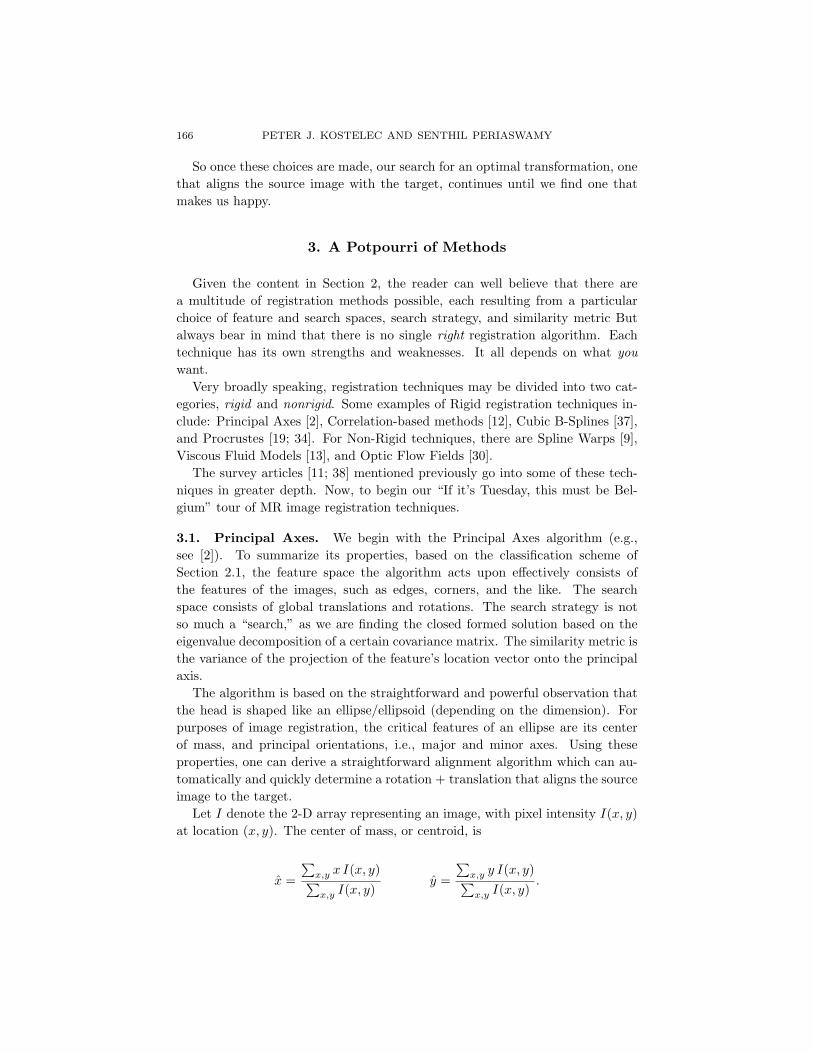
Figure 3. Principal axes. The eigenvectors E and e, corresponding to the largest

and smallest eigenvalues, respectively, indicate the directions of the major and

minor axes, respectively.

With the centroid in hand, we form the covariance matrix

C =(

c11 c12

c21 c22

),

wherec11 =

∑x,y

(x− x)2 I(x, y),

c22 =∑x,y

(y− y)2 I(x, y),

c12 =∑x,y

(x− x)(y− y) I(x, y),

c21 = c12.

The eigenvectors of C corresponding to the largest and smallest eigenvaluesindicate the direction of the major and minor axes of the ellipse, respectively.See Figure 3.

The principal axes algorithm may be described as follows. First, calculatethe centroid, and eigenvectors of the source and target images via an eigenvaluedecomposition of the covariance matrices. Next, align the centers of mass via atranslation. Next, for each image determine the angle α (Figure 3) the maximaleigenvector forms with the horizontal axis, and rotate the test image about itscenter by the difference in angles. The images are now aligned.

Figure 4 shows the procedure in action. In this example, the target image isa rotated version of the source image, with a small block missing. Subtractingthe target from the aligned source renders the missing data quite apparent.

While the principal axes algorithm is easy to implement, it does have theshortcoming that it is sensitive to missing data. As an exaggerated example,suppose the target MR image covers the entire head, while the source MR imagehas only the top half, say from the eyes on up. In this case, the anatomical


Source Target Difference

Figure 4. Principal axes: aligning axial images. The difference between the

aligned source and target images is easily apparent in the far right panel.

feature located at the centroid of the source image will differ from the anatomicalfeature located at the centroid of the target. However, be that as it may, onecan certainly use the algorithm to provide a coarse approximation to “truth.”That is, one may use rotation + translation parameters as “seed” values for moreaccurate methods.

3.2. Fourier-based correlation. Fourier-based Correlation is another methodfor performing rigid alignment of images. The feature space it uses consists ofall the pixels in the image, and its search space covers all global translations androtations. (It can also be used to find local translations and rotations [31].) Asthe name implies, the search strategy are the closed form Fourier-based meth-ods, and the similarity metric is correlation, and its variants, e.g., phase onlycorrelation [12]. As with Principal Axes, it is an automatic procedure by whichtwo images may be rigidly aligned. Furthermore, it is an efficient algorithm,courtesy of the FFT [12].

The algorithm may be described as follows. Let f(x, y) and g(x, y) denotethe source and target images, respectively. Uppercase letters will denote thefunction’s Fourier transform (FT):

f(x, y) FT⇐⇒ F (ωx, ωy), g(x, y) FT⇐⇒ G(ωx, ωy).

To clarify, (x, y) denote coordinates in the spatial domain, and (ωx, ωy) denotecoordinates in the frequency domain. Suppose the source and target are relatedby a translation (a, b) and rotation θ:

f(x, y) = g((x cos θ+y sin θ)−a, (−x sin θ+y cos θ)−b

).

Then, using properties of the Fourier transform, we have

F (ωx, ωy) = e−ı(a ωx+b ωy)G(ωx cos θ+ωy sin θ, −ωx sin θ+ωy cos θ).

By taking norms and obtaining the power spectrum, all evidence of translationby (a, b) has disappeared:

∣∣F (ωx, ωy)∣∣2 =

∣∣G(ωx cos θ+ωy sin θ, −ωx sin θ+ωy cos θ)∣∣2.


Power Spectrumcartesian coordinates polar coordinates

Sourc

eTarg

et

Figure 5. By considering the power spectra, translations vanish. Furthermore,

in polar coordinates, rotations become translations.

Note that rotating g(x, y) by θ in the spatial domain is equivalent to rotating|G(ωx, ωy)|2 by that amount in the frequency domain. By switching to polarcoordinates (setting x = r cosψ, y = r sin ψ), we have

|F (r, ψ)|2 = |G(r, ψ−θ)|2

and hence rotation in the cartesian plane becomes translation in the polar plane.See Figure 5.

We are now in a position to give an outline for the Fourier-based correlationmethod of image registration:

1. Take the discrete Fourier transform of the source image f(x) and target imageg(x).

2. Next, send the power spectra to polar coordinates land:

|F (r, ψ)|2 = |G(r, ψ−θ)|2.

3. Use your favourite correlation technique to determine the rotation angle.(Note that this is strictly a translation problem.) And then rotate the sourceimage (which is in the spatial domain) by that amount.

4. Use your favourite correlation to now determine the translation amount inthe spatial domain, between the (so far) only-rotated source image, and thetarget image.


Pattern Figure

0 20 40 600

0.5

1

1.5

2

0 20 40 600

0.5

1

1.5

2

Correlation Placement

0 20 40 600

0.5

1

1.5

2

0 20 40 600

0.5

1

1.5

2

Figure 6. We seek the pattern, shown on the top left, in the signal shown on

the top right. In the lower left, we plot the correlation values. The location of

the maximum value should indicate the location of the pattern within the signal,

but as we see in the lower right figure, placing the pattern, drawn in a thick line,

at this “maximum” location is incorrect.

Given how easy and direct the algorithm is, it would come as a surprise if therewere not any caveats associated with it.

In practice, the source and target images are probably not exactly identi-cal. This could easily result in multiple peaks, which means that the maximumpeak may not be the correct one. This phenomenon is illustrated in Figure 6.Therefore, when using correlation to determine the proper rotation and trans-lation parameters, several potential sets of parameters, e.g., corresponding tothe 4 largest correlation peaks, need to be tried. The best (in some sense, e.g.,least-squares) is the value you choose. Secondly, the images certainly should beof the same modality. Registering an MR with a PET image probably won’twork at all!

But on the bright side, along with computation efficiency, one can apply thetechnique to subregions of images and “glue” the results together. For example,one can divide the images into quarters, determine rotation and translation pa-rameters for each, all independent of each other, and then smoothly apply thesefour sets of parameters, to encompass a complete (and non-rigid) registrationof the source to target image [31]. Also, as with Principal Axes, Fourier-based


correlation may be used to achieve coarse registrations, as starting points forfancier methods.

3.3. Procrustes algorithm. The Procrustes Algorithm [19; 34] is an imageregistration algorithm that depends on the active participation of the user. Itdoes have as its inspiration a rather colourful character from Greek mythology.Especially for this reason, we feel compelled to briefly mention it.

It is a “one size fits all” algorithm: one image is compelled to fit another.The name is most appropriate for this algorithm. Procrustes is a character fromGreek mythology. He was an innkeeper who guaranteed all his beds were thecorrect length for his guests. “The top of your head will be at precisely the topedge of the bed. Similarly the soles of your feet will be at the bottom edge.”And for his (unfortunate) guests of varying heights, they were. Procrustes wouldemploy some rather gruesome measures to make his claim true. Ouch.

As already mentioned, the algorithm depends on human intervention. Quitesimply, the user identifies common features or landmarks in the images (so this isthe feature space) and, by rigid rotation and translation (the search space), forcesa registration that respects these landmarks. In a perfect world, to determinethe proper rotation and translation parameters, three pairs of landmarks wouldsuffice. The rotation parameters place the images in the same orientation, thetranslation parameters, well, translate the images into alignment.

But we do not inhabit a perfect world. The slightest variation in distance be-tween any homologous pair represents an error in landmark identification whichcannot be reconciled with rigid body motions. And so we need to compromise.(Procrustes would have difficulty understanding this. While his enthusiasm forachieving a perfect fit is admirable, it could result in some uncomfortable sideeffects for the patients.) Lacking a perfect match, the similarity metric employedis instead the mean squared distance between homologous landmarks when com-puting the six rigid body parameters. The search strategy is to minimize vialeast-squares.

The good news is that this can be accomplished efficiently. A closed formsolution exists, in fact. However, the not so good news is that it depends on theaccurate identification of landmarks. If you say that the anatomical feature atPoint A1 in source image A really corresponds with the anatomical feature atPoint B1 in the target image B, you had better be right. And being right takestime, especially since the slightest deviation is a source of error.

3.4. AIR: automated image registration. AIR is a sophisticated andpowerful image registration algorithm. Developed by Woods et al [41; 42; 43],the feature space it uses consists of all the pixels in the image, and the searchspace consists of up to fifth-order polynomials in spatial coordinates x, y (and z,if 3-D), involving as many as 168 parameters. The goal is to define a single,global transformation. We outline some of AIR’s characteristics:


• AIR is a fully automated algorithm.• Unlike the algorithms so far discussed, AIR can be used in multi-modal situ-

ations.• AIR does not depend on landmark identification.• AIR uses overall similarity between images.• AIR is iterative.

It is a robust and versatile algorithm. The fact that AIR software is publiclyavailable [1] has only added to its widespread use.

AIR is based on the following assumption. If two images, acquired the sameway (i.e., same modality) are perfectly aligned, then the ratio of one image toanother, on a pixel by pixel basis, ought to be fairly uniform across voxels. Ifregistration is not spot on correct, then there would be a substantial degree ofnonuniformity in ratios. Ergo, to register the two images, compute the standarddeviation of the ratio, and minimize it. This error function is called the “ratioof image uniformity”, or RIU. The algorithm’s search strategy is based on gra-dient descent, and the similarity metric is actually a normalized version of theRIU between the two volumes. An iterative procedure is used to minimize thenormalized RIU in which the registration parameters (three rotation and threetranslation terms) with the largest partial derivative is adjusted in each iteration[41].

Since we are dealing with ratios and not pixel intensities themselves, it is thisidea of using the ratios to register images which provides us with the flexibilityto align images of different modalities.

Suppose we are in the situation where we want to align an MR to a PETimage. On the face of it, the ratios will not be uniform across the images.Different tissue types will have different ratios. However, and this is key, withina given tissue type, the ratio ought to be fairly uniform when the images areregistered. Therefore, what you want to do is maximize the uniformity withinthe tissue type, where the tissue-typing is based on the MRI voxel intensity.This requires two modifications of the original algorithm [43]. First, one hasto manually edit the scalp, skull and meninges from the MR image since thesefeatures are not present in the PET image. The second modification consists offirst performing a histogram matching. Denote the two images to be histogrammatched as f1 ( ·) and f2 ( ·), and c2( · ) as the sampled cumulative distributionfunction of image f2( ·). The histogram of f2( ·) is made to match that of f1( ·)by mapping each pixel f1(x, y) to c2 (f1(x, y)), between the MR and PET images(with 256 bins), followed by a segmentation of the images according to the 256bin values. Each of the segmented MR and PET images (with corresponding binvalues) are then registered separately.

In terms of implementation, both the within-modality and cross-modalityversions of the algorithm, the registration is performed on sub-sampled images,in decreasing order of sub-sampling.


There are a number of things to keep in mind. AIR’s global approach impliesthe transformation will be consistent throughout the entire image volume. How-ever, this does introduce the possibility of obtaining an unstable transformation,especially near the image boundaries. And small and/or local perturbations mayresult in disproportionate changes in the global transformation. And the AIRalgorithm is also computationally intensive. It is not easy, after all, to minimizethe standard deviation of the ratios. However, the algorithm does perform wellwith noisy data [36].

3.5. Mutual information based techniques. Mutual Information [39] is anerror metric (or similarity metric) used in image registration based on ideas fromInformation Theory. Mutual Information uses the pixel intensities themselves.The strategy is this: minimize the information content of the difference image,i.e., the content of target-source.

Consider Figure 7. The particular example is a bit of a cheat, but it illustratesthe point. In the top row we have two axial images. They are the source

Figure 7. The philosophy behind Mutual Information. The source is the top left

image, and the target is the top right. The difference image between the aligned

source and target (lower left) looks nearly completely blank. Some structure

might be vaguely visible, but not nearly as much as the difference image resulting

translating the aligned source by 1 pixel (lower right).


and target images. The image on the lower left is the difference between thealigned source and target. Since the pixel intensities of the source and targetare nearly identical, the difference image is basically blank. Now suppose wetake the aligned source and translate it by one pixel. In the resulting differenceimage, the boundary of the skull is quite obvious. Whereas in the first differenceimage one has to “hunt” for features (and fail to find any), in the second we donot. Features stand out. So, in a sense, the second difference image has moreinformation than that first: we see a shape. Mutual Information wants thatdifference image to have as little information as possible.

To go a little further, let us begin with the question: how well does one imageexplain, or “predict”, another? We use a joint probability distribution. Letp(a, b) denote the probability that a pixel value a in the source and b in thetarget occurs, for all a and b. We estimate the joint probability distribution bymaking a joint histogram of pixel values. When two images are in alignment, thecorresponding anatomical area overlap, and hence there are lots of high values.In misalignment, anatomical areas are mixed up, e.g., brain over skin, and thisresults in a somewhat more dispersed joint histogram. See Figures 8 and 9.

What we want to do is make the “crispiest” joint probability distributionpossible. Let I(A,B) denote the Mutual Information of two images A and B.This can be defined in terms of the entropies (i.e., “How dispersed is the jointprobability distribution?”) H(A), H(B) and H(A,B):

I(A, B) = H(A)+H(B)−H(A, B) =∑

x∈A, y∈B

p(x, y) log2

(p(x, y)

p(x)p(y)

).

Therefore, to maximize their mutual information I(A,B), to get image A totell us as much as possible about B, we need to minimize the entropy H(A,B).The reader is encouraged to read the seminal paper by Viola et al. [39] for fur-ther information regarding exactly how the entropy H(A,B) is minimized. Inbrief, [39] use a stochastic analog of the gradient descent technique to maximizeI(A,B), after first approximating the derivatives of the mutual information errormeasure. In order to obtain these derivatives, the probability density functionsare approximated by a sum of Gaussians using the Parzen-window method [16](after this approximation, the derivatives can be obtained analytically). Thegeometric distortion model used is global affine. In general, the various im-plementations differ in the minimization technique. For example, Collignon etal. [14] use Powell’s method for the minimization.

In the final analysis, we find that Mutual Information is quite good in multi-modal situations. However, it is computationally very expensive, as well as beingsensitive to the how the interpolation is done, e.g., the minimum found may notbe the correct/optimal one.


A functional image Perfect alignment

One pixel off Three pixels off

Figure 8. Joint histograms of identical source and target images. No registration

is necessary to align them. The resulting joint histogram is a diagonal line.

Translating by 1 pixel significantly disperses the diagonal (lower left), and by 3

pixels, further still (lower right).

3.6. Optic flow fields. This registration technique [30] borrows tools from dif-ferential flow estimation. The underlying philosophical principle of the algorithmis that we want to flow from the source to the target. Think of an air bubblethat is rising to the surface of a lake. The bubble’s surface smoothly bends andflexes this way and that as it floats upward. The source and target images aretwo snapshots taken of the rising bubble. Starting from the two snapshots, thealgorithm determines the deformations that occur when going from source totarget. The source image is the bubble at t = 0, and the target image is thebubble at t = 1. What happened between 0 and 1 ?

The highlights of this technique are:

• The technique based on differential flow estimation.• Idea: Want to flow from the source image to reference image.• The procedure is fully automated.• Uses an affine model.• Allows for intensity variations between the source and target images.


Source Target

Aligned One pixel off

Figure 9. Joint histograms of different source and target images. While not

strictly a diagonal line, the joint histogram of the aligned source and target

images is relatively narrow (lower left). Translating by one pixel significantly

disperses the diagonal (lower right).

Full details and results of the algorithm may be found in [30]. Since the modelis very straightforward, we will delve a little deeper into this algorithm than wehave so far with the previous algorithms discussed. It can be considered as anexample of how, beginning with basic principles, a registration technique is born.

Our starting point is the general form of a 2-D affine transformation:[

x1

y1

]=

[m1 m2

m3 m4

][x

y

]+

[m5

m6

]

where x, y denote spatial coordinates in the source image and x1, y1 denote spa-tial coordinates in the target. Depending on the values m1, m2, m3 and m4,certain well known geometric transformations can result (see Figure 10).

Now recall our description at the beginning of this section, that of a bubblerising through the water. We took two snapshots, one at t = 0, and one att = 1, of the same bubble. Hence it is reasonable to have a single function, withtemporal variable t, represent the bubble at time t.

With this in mind, let f(x, y, t), f(x, y, t−1) represent the source and targetimages, respectively. To further simplify the model, at least for the moment, we


original:

0 11 0

rotation:

cos θ sin θ

− sin θ cos θ

scaling:

m1 00 m4

shear:

1 m2

m3 1

Figure 10. A smattering of linear transformations.

will make the “Brightness-Constancy” assumption: identical anatomical featuresin both images will have the same pixel intensity. That is, we are not allowingfor the possibility that, say, the left eye in the MR source image to be brighter ordarker than the left eye in the MR target image. Before tackling more difficultissues later, we want to ensure that only an affine transformation, and nothingelse, is required to mold the source into the target.

Using the notation we have just introduced (which we will slightly abuse now),we have the situation:

f(x, y, t) = f(m1x+m2y+m5, m3x+m4y+m6, t−1) (3–1)


We use a least squares approach to estimate the parameters ~m = (m1 . . .m6)T

in (3–1). Now the function we really want to minimize is:

E(~m) =∑

x,y ∈Ω

(f(x, y, t)−f(m1x+m2y+m5, m3x+m4y+m6, t−1)

)2 (3–2)

where Ω denotes the region of interest. However, the fact that E(~m) is not linearmeans that minimizing will be tricky. So we take an easy way out and insteadtake its truncated, first-order Taylor series expansion. Letting

k = ft +xfx +yfy,

~c = (xfx yfx xfy yfy fx fy)T,

(3–3)

where the subscripts denote partial derivatives, we eventually arrive at this muchmore reasonable error function:

E(~m) =∑

x,y ∈Ω

(k−~cT ~m

)2. (3–4)

To minimize (3–4), we differentiate with respect to ~m:

dE

d~m=

∑

Ω

−2~c(k−~cT ~m

),

set equal to 0, and solve for the model parameters to obtain:

~m =

(∑

Ω

~c~cT

)−1(∑

Ω

~ck

). (3–5)

And lo! we have determined ~m. However, there is a caveat. We are assumingthat the 6×6 matrix

(∑Ω ~c~cT

)in (3–5) is, in fact, invertible. We can usually

guarantee this by making sure that the spatial region Ω is large enough to havesufficient image content, e.g., we would want some “interesting” features in Ω likeedges, and not simply a “bland” area. The parameters ~m are for the region Ω.

In terms of actually implementation, the parameters ~m are estimated locally,for different spatial neighborhoods. By applying this algorithm in a multi-scalefashion, it is possible to capture large motions. (See [30] for details.) This isillustrated in Figure 11, in the case where the target image is a syntheticallywarped version of the source image.

Editorial. As an aside, we mention that doing an experiment such as this, reg-istering an image with a warped version of itself is not altogether silly. If analgorithm being developed fails in an ideal test case such as this, chances arevery good that it will fail for genuinely different images. However, to make a“fair” ideal test, the method of warping the image should be independent of theregistration method. For example, if the registration algorithm is to determinean affine transform, do not warp the image using an affine transform. Use someother method, e.g., apply Bookstein’s thin-plate splines [9].


Source Target Registered result

Figure 11. Flowing from source to target: An “ideal” experiment.

The optic flow model can next be modified to account for differences of con-trast and brightness between the two images with the addition of two new pa-rameters, m7 for contrast, and m8 for brightness. The new version of (3–1) is

m7f(x, y, t)+m8 = f(m1x+m2y+m5,m3x+m4y+m6, t−1). (3–6)

We are also assuming that, in addition to the affine parameters, the brightnessand contrast parameters are constant within small spatial neighborhoods.

Minimizing the least squares error as before, using a first-order Taylor seriesexpansion, gives a solution identical in form to (3–5) except that this time

k = ft−f +xfx +yfy,

~c = (xfx yfx xfy yfy fx fy −f −1)T ;(3–7)

compare equations (3–3).Now, we have been working under the assumption that the affine and con-

trast/brightness parameters are constant within some small spatial neighbor-hood. This introduces two conflicting conditions.

Recall(∑

Ω ~c~cT). This matrix needs to have an inverse. As was mentioned

earlier, this can be arranged by considering a large enough region Ω, i.e., a regionwith sufficient image content. However, the larger the area, the less likely it isthat the brightness constancy assumption holds. Think about it: image contentcan be edges, and edges can have very different intensities, when compared withsurrounding tissue.

Fortunately, the model can be modified one more time. Instead of a singleerror function (3–4), we can instead consider the sum of two errors:

E(~m) = Eb(~m)+Es(~m) (3–8)

where

Eb(~m) =(k−~cT ~m

)2


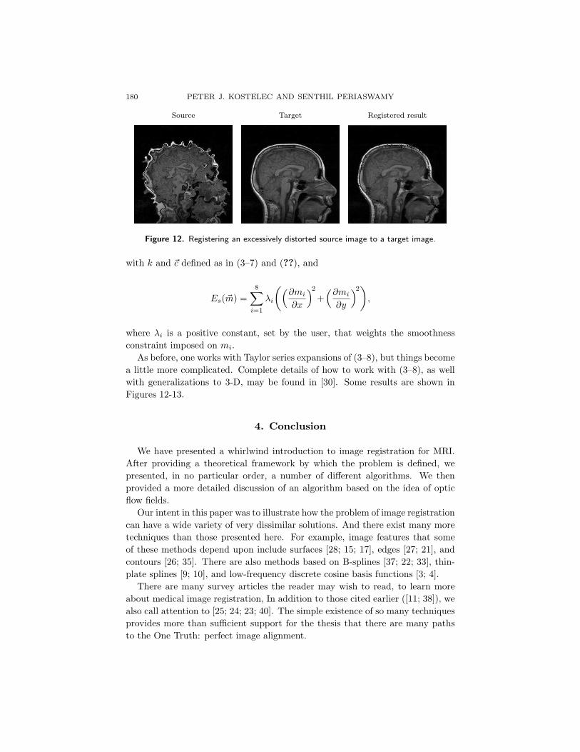
Source Target Registered result

Figure 12. Registering an excessively distorted source image to a target image.

with k and ~c defined as in (3–7) and (??), and

Es(~m) =8∑

i=1

λi

((∂mi

∂x

)2

+(

∂mi

∂y

)2)

,

where λi is a positive constant, set by the user, that weights the smoothnessconstraint imposed on mi.

As before, one works with Taylor series expansions of (3–8), but things becomea little more complicated. Complete details of how to work with (3–8), as wellwith generalizations to 3-D, may be found in [30]. Some results are shown inFigures 12-13.

4. Conclusion

We have presented a whirlwind introduction to image registration for MRI.After providing a theoretical framework by which the problem is defined, wepresented, in no particular order, a number of different algorithms. We thenprovided a more detailed discussion of an algorithm based on the idea of opticflow fields.

Our intent in this paper was to illustrate how the problem of image registrationcan have a wide variety of very dissimilar solutions. And there exist many moretechniques than those presented here. For example, image features that someof these methods depend upon include surfaces [28; 15; 17], edges [27; 21], andcontours [26; 35]. There are also methods based on B-splines [37; 22; 33], thin-plate splines [9; 10], and low-frequency discrete cosine basis functions [3; 4].

There are many survey articles the reader may wish to read, to learn moreabout medical image registration, In addition to those cited earlier ([11; 38]), wealso call attention to [25; 24; 23; 40]. The simple existence of so many techniquesprovides more than sufficient support for the thesis that there are many pathsto the One Truth: perfect image alignment.


Source Target

Registered edge difference Registered result

Figure 13. Registering two different clinical images. The lower left image shows

how the edges of the registered source compare with the target’s edges. The

lower right image shows the registered source itself, after it has undergone both

geometric and intensity-correction transformations.

References

[1] The homepage for the AIR (“Automated Image Registration”) software package ishttp://bishopw.loni.ucla.edu/AIR5/.

[2] N. Alpert, J. Bradshaw, D. Kennedy, and J. Correia, The principal axes transfor-mation: a method for image registration, J. Nuclear Medicine 31 (1990), 1717–1722.

[3] J. Ashburner and K. J. Friston, Multimodal image coregistration and partitioning:a unified framework, NeuroImage 6:3 (1997), 209–217.

[4] J. Ashburner, P. Neelin, D. L. Collins, A. C. Evans and K. J. Friston, Incorporatingprior knowledge into image registration, NeuroImage 6 (1997), 344–352.

[5] Peter A. Bandettini, Eric C. Wong, R. Scott Hinks, Ronald S. Tikofsky, and JamesS. Hyde, Time course EPI of human brain function during task activation, MagneticResonance in Medicine 25 (1992), 390–397.

[6] P. A. Bandettini, E. C. Wong, J. R. Binder, S. M. Rao, A. Jesmanowicz, E. Aaron,T. Lowry, H. Forster, R. S. Hinks, J. S. Hyde, Functional MRI using the BOLDapproach: Dynamics and data analysis techniques, pp. 335–349 in Perfusion andDiffusion: Magnetic Resonance Imaging, edited by D. LeBihan and B. Rosen, RavenPress, New York, 1995.

[7] M. Betke, H. Hong, and J. P. Ko, Automatic 3D registration of lung surfaces in com-puted tomography scans, pp. 725–733 Fourth International Conference on Medical


Image Computing and Computer-Assisted Intervention, Utrecht, The Netherlands,October 2001.

[8] Amanda Bischoff-Grethe, Shawnette M. Proper, Hui Mao, Karen A. Daniels, andGregory S. Berns, Conscious and unconscious processing of nonverbal predictabilityin Wernicke’s Area, Journal of Neuroscience 20:5 (March 2000), 1975–1981.

[9] F. L. Bookstein, Principal Warps: Thin-plate splines and the decomposition ofdeformations, IEEE Transactions on Pattern Analysis and Machine Intelligence,11:6 (June 1989), 567–585.

[10] F. L. Bookstein, Thing-plate splines and the atlas problem for biomedical images,Information Processing in Medical Imaging, July 1991, 326–342.

[11] Leslie G. Brown, A Survey of Image Registration Techniques, ACM ComputingSurveys, 24:4 (December 1992), 325–376.

[12] E. D. Castro and C. Morandi, Registration of translated and rotated images usingfinite Fourier transforms, IEEE Trans. Pattern Anal. Mach. Intell., PAMI-9 (1987),700–703.

[13] G.E. Christensen, R.D. Rabbit, and M.I. Miller, A deformable neuroanatomytextbook based on viscous fluid mechanics, pp. 211–216 in Proceedings of the 1993Conference on Information Sciences and Systems, Johns Hopkins University, March1995.

[14] A. Collignon and F. Maes and D. Delaere and D. Vandermeulen, P. Suetens andG. Marchal, Automated multimodality image registration using information theory,pp. 263–274 in Information Processing in Medical Imaging, edited by Y. Bizais, C.Barillot, and R. Di Paolo, Kluwer, Dordrecht, 1995.

[15] A. M. Dale, B. Fischl, and M. I. Sereno, Cortical surface-based analysis, I:Segmentation and surface reconstruction, NeuroImage 9:2 (Feb 1999), 179–194.

[16] R. O. Duda and P.E. Hart, Pattern classification and scene analysis, Wiley, NewYork, 1973.

[17] B. Fischl, M. I. Sereno, and A. M. Dale, Cortical surface-based analysis, II:Inflation, flattening, and a surface-based coordinate system, NeuroImage 9:2 (Feb.1999), 195–207.

[18] R. S. J. Frackowiak, K. J. Friston, C. D. Frith, R. J. Dolan, and J. C. Mazziotta,Human Brain Function, Academic Press, San Diego, 1997.

[19] J. R. Hurley and R. B. Cattell, The PROCRUSTES program: Producing directrotation to test a hypothesized factor structure, Behav. Sci. 7 (1962), 258–262.

[20] P. Janata, B. Tillman, and J. J. Bharucha, Listening to polyphonic music recruitsdomain-general attention and working memory circuits, Cognitive, Affective, andBehavioral Neuroscience, 2:2 (2002), 121–140.

[21] W. S. Kerwin and C. Yuan, Active edge maps for medical image registration,pp. 516–526 in Proceedings of SPIE – The International Society for Optical Engi-neering, July 2001.

[22] P. J. Kostelec, J. B. Weaver, and D. M. Healy, Jr., Multiresolution Elastic ImageRegistration, Medical Physics, 25:9 (1998), 1593–1604.

[23] H. Lester and S. Arridge, A Survey of Hierarchical Non-linear Medical ImagingRegistration, Pattern Recognition 32:1 (1999), 129–149.


[24] J. B. Antoine Maintz and Max A. Viergever, A Survey of Medical Image Regis-tration, Medical Image Analysis 2:1 (1998), 1–36.

[25] C. R. Maurer Jr. and J. M. Fitzpatrick, A Review of Medical Image Registra-tion, chapter in Interactive Image-Guided Neurosurgery, American Association ofNeurological Surgeons, Park Ridge, IL, 1993.

[26] G. Medioni and R. Nevatia, Matching images using linear features, IEEE Trans.Pattern Anal. Mach. Intell. 6:6 (Nov. 1984), 675–685.

[27] M. L. Nack, Rectification and registration of digital images and the effect ofcloud detection, pp. 12–23 in Machine Processing of Remotely Sensed Data, WestLafayette, IN, June 1977.

[28] C. A. Pelizarri, G. T. Y. Chen, D. R. Spelbring, R. R. Weichselbaum, and C. T.Chen, Accurate three-dimensional registration of CT, PET and/or MR images ofthe brain, J. Computer Assisted Tomography, 13:1 (1989), 20–26.

[29] Senthil Periaswamy, www.cs.dartmouth.edu/ sp.

[30] Senthil Periaswamy and Hany Farid, Elastic registration in the presence ofintensity variations, to appear in IEEE Transactions in Medical Imaging.

[31] S. Periaswamy, J. B. Weaver, D. M. Healy, Jr., and P. J. Kostelec, Automatedmultiscale elastic image registration using correlation, pp. 828–838 in Proceedings ofthe SPIE – The International Society for Optical Engineering 3661, 1999.

[32] William K. Pratt, Digital signal processing, Wiley, New York, 1991.

[33] D. Rueckert, L. I. Sonoda, C. Hayes, D. L. G. Hill, M. O. Leach, and D. J.Hawkes, Non-rigid registration using free-form deformations: Application to breastMR images, IEEE Trans. Medical Imaging, 18:8 (August 1999), 712–721.

[34] P. H. Schonemann, A generalized solution of the orthogonal Procrustes problem,Psychometrika, 31:1 (1966), 1–10.

[35] Wen-Shiang V. Shih, Wei-Chung Lin, and Chin-Tu Chen, Contour-model-guidednonlinear deformation model for intersubject image registration, pp. 611–620 inProceedings of SPIE - The International Society for Optical Engineering 3034, April1997.

[36] Arthur W. Toga and John C. Mazziotta (eds.), Brain mapping: the methods,Academic Press, San Diego, 1996.

[37] M. Unser, A. Aldroubi and C. Gerfen, A multiresolution image registration pro-cedure using spline pyramids, pp. 160–170 Proceedings of the SPIE – MathematicalImaging: Wavelets and Applications in Signal and Image Processing 2034, 1993.

[38] P. A. Van den Elsen, E. J. D. Pol, M. A. Viergever, Medical Image Matching - areview with classification, IEEE Engineering in Medicine and Biology 12:1 (1993),26–39,

[39] P. Viola and W. M. Wells, III, Alignment by maximization of mutual information,pp. 16–23 in International Conf. on Computer Vision, IEEE Computer SocietyPress, 1995.

[40] J. West, J. Fitzpatrick, M. Wang, B. Dawant, C. Maurer, R. Kessler, andR. Maciunas, Comparison and evaluation of retrospective intermodality imageregistration techniques, pp. 332–347 Proceedings of the SPIE - The InternationalSociety for Optical Engineering, Newport Beach, CA., 1996.


[41] R. P. Woods, S. R. Cherry, and J. C. Mazziotta, Rapid automated algorithm foralignment and reslicing PET images, J. Computer Assisted Tomography 16 (1992),620–633.

[42] R. P. Woods, S. T. Grafton, C. J. Holmes, S. R. Cherry, and J. C. Mazziotta,Automated image registration, I: General methods and intrasubject, intramodalityvalidation, J. Computer Assisted Tomography 22 (1998), 141–154.

[43] R. P. Woods, J. C. Mazziotta, and S. R. Cherry, MRI-PET registration withautomated algorithm, J. Comp. Assisted Tomography, 17:4 (1993) 536–546.

Peter J. KostelecDepartment of MathematicsDartmouth CollegeHanover, NH 03755United States

[email protected]

Senthil PeriaswamyDepartment of Computer ScienceDartmouth CollegeHanover, NH 03755United States

[email protected]

Documents

Image Registration for MRI - MSRIlibrary.msri.org/books/Book46/files/07kostelec.pdf · Image Registration for MRI ... a circular feature in the ﬁrst slice appears ... Do we assume