Embed Size (px)
Citation preview
i
Image Processing for Synthetic Aperture Radar System on
Light-weight Drone
Senior Honors Thesis
Presented in Partial Fulfillment of the Requirements for Graduation with Distinction in the
College of Engineering of The Ohio State University
By
Shiqi Yang
Department of Electrical and Computer Engineering
Advisor:
Professor Lee Potter
Department of Electrical and Computer Engineering

ii
Abstract
This project focuses on the implementation of image processing software for a drone-based
synthetic aperture radar (SAR) system. The drone-SAR system is under development by a
student design team. The specific contributions in this thesis are two stages of software
development. In the first part, to achieve a basic image formation function, we implemented and
demonstrated backprojection imaging using radar data and global positioning system (GPS) data
collected by the team. In the second part, we researched and implemented an autofocus
algorithm, in order to generate high-resolution images in the inevitable presence of measurement
errors greater than one-quarter wavelength.

iii
Acknowledgements
The author would like to thank his drone-SAR project team, which includes David Giffin, Sarah
Greenbaum, Joy Smith, Brandi Downs, Arron Pycraft, Luke Smith, Daniel Wharton and Jingong
Huang, who supported the author for the completion of this thesis project. The author would also
like to thank Professor Potter for his mentoring and helpful advice, which ensured the successful
completion of this thesis project and this thesis.
iv
Table of Contents Abstract ......................................................................................................................................... ii
Acknowledgments ........................................................................................................................ iii
List of Tables ............................................................................................................................... vi
List of Figures .............................................................................................................................. vi
CHAPTER 1: Introduction ..........................................................................................................1
1.1 Goals ....................................................................................................................................1
1.2 Teamwork ............................................................................................................................1
1.3 Standards and Regulations ...................................................................................................2
1.4 Specific Contributions .........................................................................................................3
1.5 Outline of Thesis ..................................................................................................................3
CHAPTER 2: Backprojection Algorithm ...................................................................................4
2.1 FMCW & Stretch Processing...............................................................................................4
2.1.1 Signal Model .............................................................................................................4
2.1.2 Stretch Processing .....................................................................................................6
2.1.3 Hardware Implementation of Stretch Processing .....................................................8
2.2 Backprojection Algorithm ...................................................................................................9
2.2.1 Signal Model for Single Pulse ..................................................................................9
2.2.2 Fourier Analysis ......................................................................................................10
2.2.3 Discrete-Time Signal Model for Single Pulse ........................................................11
2.2.4 Performance of Radar System ................................................................................13
2.2.5 Range Profile for Single Pulse ................................................................................14
2.2.6 Backprojection ........................................................................................................17
CHAPTER 3: Autofocus Algorithm ..........................................................................................19
3.1 General Signal Model ........................................................................................................19
3.2 Signal Model for Single Pulse Phase Correction ...............................................................21
3.3 Geometric Interpretation for Single Pulse Phase Correction .............................................22
3.4 Phase Optimization for Single Pulse Phase Correction .....................................................23
CHAPTER 4: Results .................................................................................................................27
4.1 Software Products ..............................................................................................................27
4.2 Experiment Results ............................................................................................................29
4.2.1 Backprojection Experiment ....................................................................................29

v
4.2.2 Autofocus Experiment ............................................................................................31
4.2.3 Drone-SAR Experiment ..........................................................................................33
CHAPTER 5: Errors and Analysis ...........................................................................................35
5.1 Ghost Peak in Near-field ....................................................................................................35
5.2 IQ Imbalance and IQ Correction........................................................................................36
5.2.1 Influence of IQ Imbalance ......................................................................................36
5.2.2 IQ Correction ..........................................................................................................39
5.3 Linear Range Error ............................................................................................................41
5.4 Motion Error .......................................................................................................................43
CHAPTER 6: Conclusion and Future Works ..........................................................................49
CHAPTER 7: Reference .............................................................................................................50
vi
List of Tables Table 1: Drone-SAR Project Team Division ..............................................................................2
Table 2: Regulations and Team Decisions ..................................................................................2
Table 3: Backprojection Parameter List ....................................................................................16
List of Figures
Figure 1: FMCW Radar Model ...................................................................................................4
Figure 2: FMCW Frequencies .....................................................................................................6
Figure 2(a): Frequency vs. Time for Transmission and Received Signals .........................6
Figure 2(b): Beat Frequency ...............................................................................................6
Figure 3: Radar Receiver Architecture ........................................................................................8
Figure 4: Radar Detectable Range ............................................................................................10
Figure 5: Graphical Representation of Radar Parameters .........................................................13
Figure 6: Range Line Example ..................................................................................................16
Figure 7: Backprojection Graphical Interpretation ....................................................................18
Figure 8: Autofocus Geometric Interpretation for Single Pulse Phase Correction ....................22
Figure 9: Software Processing Flow ..........................................................................................27
Figure 9(a): Data Simulator Processing Flow ....................................................................27
Figure 9(b): Image Processing Software Processing Flow ................................................27
Figure 10: Backprojection Experiment ......................................................................................30
Figure 10(a): Physical Setup of Reflectors ........................................................................30
Figure 10(b): Conceptual Graph ........................................................................................30
Figure 10(c): Simulated SAR Image ..................................................................................30
Figure 10(d): Experimental SAR Image ............................................................................30
Figure 11: Autofocus Experiment ..............................................................................................32
Figure 11(a): Conceptual Graph ........................................................................................32
Figure 11(b): Simulated SAR Image with Phase Errors ....................................................32
Figure 11(c): Simulated SAR Image with Autofocus ........................................................32
Figure 12: Drone-SAR System ..................................................................................................32
Figure 13: Drone-SAR Experiment ............................................................................................33
Figure 13(a): Conceptual Graph in a Bird’s Eye View ......................................................33
Figure 13(b): Simulated SAR Image .................................................................................33

vii
Figure 13(c): Experimental SAR Image without Autofocus .............................................33
Figure 13(d): Experimental SAR Image with Autofocus ..................................................33
Figure 14: Experimental Range Line in Anechoic Chamber .....................................................35
Figure 15: Range Line Analysis ................................................................................................38
Figure 15(a): Range Line Associated with Signal 𝑦 ..........................................................38
Figure 15(b): Range Line Associated with Signal ..........................................................38
Figure 16: IQ Correction Simulation ........................................................................................40
Figure 16(a): I and Q Signals in Ideal Case .......................................................................40
Figure 16(b): Imbalanced I and Q Signals .........................................................................40
Figure 16(c): IQ Correction Outputs..................................................................................40
Figure 17: Relationship between Range Error and Reflector Absolute Range Position ...........42
Figure 18: Influence of the Motion Error ..................................................................................44
Figure 18(a): Geometric Representation of the Motion Error ...........................................44
Figure 18(b): Influence of the Motion Error on the Range Profile ....................................44
Figure 19: Influence of the Motion Error on Multiple Pixels ....................................................47

1
CHAPTER 1: Introduction
1.1 Goals
A synthetic aperture radar (SAR) system is capable of providing vision under special
circumstances when optical systems may fail: at night, through clouds, though fog, through dust
and etc [1]. In autumn of 2017, a SAR project team in the department of Electrical and Computer
Engineering at The Ohio State University (OSU) built a C-band SAR system on a rail. The
system could generate images of reflectivity at a range of 7 meters [2]. Based on previous work
in autumn 2017, a new SAR project team was formed in spring of 2018, aiming at making an X-
band SAR system on a small drone. The new X-band SAR system needs to have a minimum
detectable range of 80 meters and it must generate a 100 × 100 pixel image with a resolution
less than one meter. The cost of the system should not exceed $10,000 and the weight of the
system is kept on the order of few kilograms [3].
1.2 Teamwork
The drone-SAR project team is divided into four groups. People in the first group focus
on system integration and drone operation; the second group is responsible for GPS test and data
collection; people in the third group focus on X-band radar evaluation and radar data collection;
the main task for people in the last group is software development for image processing in the
system. Table 1 shows the team division. The team carried out project management through
Google Drive and GitHub. During the project cycle, weekly meetings were hold to report the
progress.

2
1.3 Standards and Regulations
In this project, the drone-SAR system must satisfy regulations from the Federal Aviation
Administration (FAA) [4], the Federal Communications Commission (FCC) [5] and OSU [6].
Table 2 [3 ] shows detailed information about constraints from different regulations to the drone-
SAR project. In order to satisfy FAA, FCC and OSU regulations, the team made a series of
decisions, which were also included in Table 2.
Table 1: Drone-SAR Project Team Division
Table 2: Regulations and Team Decisions

3
1.4 Specific Contribution
This report focuses on image processing for the drone-SAR system. The goal is to
compute 2-D high-resolution images as the output of the system based on information from other
modules. In the first stage, we implement the backprojection algorithm [7] to achieve a
fundamental image formation function in the drone-SAR system.
In reality, SAR images would be smeared or blurred because of non-ideal factors, such as
motion measurement errors, noises, unstable behaviors of the radar system, etc. In order to form
high-quality images from drone-SAR system without extra hardware cost, application of
autofocus algorithm is necessary. In the second stage, a time-domain autofocus is integrated into
the software [8].
1.5 Outline of Thesis
In Chapter 2 of this report, we performed analysis to operating principles of the X-band
radar in and introduced backprojection algorithm for image construction. In Chapter 3, we
presented a time-domain autofocus algorithm to enhance the quality of SAR image. We
demonstrated the project results in Chapter 4 and carried out result analysis in Chapter 5. In
Chapter 6, we showed conclusions from this project and provided suggestions to future works.
4
CHAPTER 2: Backprojection Algorithm
2.1 FMCW & Stretch Processing
2.1.1 Signal Model
Frequency modulation continuous wave (FMCW) is a common technique applied in
radar systems. Stretch processing [9] is a signal processing algorithm for a FMCW radar system.
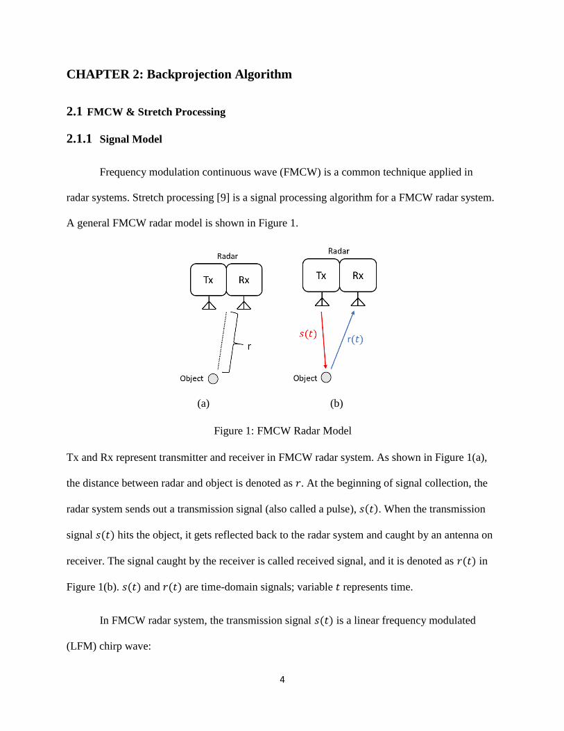
A general FMCW radar model is shown in Figure 1.
Tx and Rx represent transmitter and receiver in FMCW radar system. As shown in Figure 1(a),
the distance between radar and object is denoted as 𝑟. At the beginning of signal collection, the
radar system sends out a transmission signal (also called a pulse), 𝑠(𝑡). When the transmission
signal 𝑠(𝑡) hits the object, it gets reflected back to the radar system and caught by an antenna on
receiver. The signal caught by the receiver is called received signal, and it is denoted as 𝑟(𝑡) in
Figure 1(b). 𝑠(𝑡) and 𝑟(𝑡) are time-domain signals; variable 𝑡 represents time.
In FMCW radar system, the transmission signal 𝑠(𝑡) is a linear frequency modulated
(LFM) chirp wave:
(a) (b)
Figure 1: FMCW Radar Model

5
1. An image can be simply interpreted as a collection of pixels and each pixel has a certain value of strength. In
this project, for image construction, the key is to find A(r).
2. The one-way propagation loss related to 1
𝑟2 is ignored in the derivations of equations (2) and (3)
𝑠(𝑡) = cos((𝜔𝑐 + 𝛼𝑡) ∙ 𝑡) , −𝑇
2≤ 𝑡 ≤
𝑇
2. (1)
Several parameters are associated with the property of radar system:
𝜔𝑐 Carrier Frequency (rad/sec)
𝑓𝑐 Carrier Frequency (Hz)
𝑇 Sweep Time (s)
𝐵𝑊 Bandwidth (Hz)
𝛼 Chirp Rate (rad/𝑠2)
𝑐 Speed of propagation (m/s)
Relationships among these parameters are:
𝜔𝑐 = 2𝜋𝑓𝑐
𝛼 =2𝜋 ∙ 𝐵𝑊
𝑇
The received signal 𝑟(𝑡) is a time-delayed and scaled version of 𝑠(𝑡). According to Figure 1(a),
corresponding time delay associated with the distance, 𝑟, is:
𝑡𝑑𝑒𝑙𝑎𝑦 =2𝑟
𝑐 (unit: sec)
where 2𝑟 means that the radar signal travels a distance of 𝑟 to hit the object and travels another 𝑟
to come back to receiver. 𝐴(𝑟) represents reflection signal at a distance 𝑟 away from the radar1
and it is called “range profile”. In the ideal case, the received signal can be represented as
follows2:
𝑟(𝑡) = 𝐴(𝑟) ∙ 𝑠(𝑡 − 𝑡𝑑𝑒𝑙𝑎𝑦) = 𝐴(𝑟) ∙ 𝑠 (𝑡 −2𝑟
𝑐)
𝑟(𝑡) = 𝐴(𝑟) ∙ cos (𝜔𝑐 (𝑡 −2𝑟
𝑐) + 𝛼 (𝑡 −
2𝑟
𝑐)2
), −𝑇
2≤ 𝑡 ≤
𝑇
2 (2)
6
However, when nonideal factors are considered, they influence the received signal. At a distance
𝑟 away from radar, we model the influences from nonideal factors by an attenuation 𝑝(𝑟) and a
phase shift 𝜙𝑟. As a result, the nonideal received signal under influences of noises can be
expressed as:
𝑟(𝑡) = 𝐴(𝑟) ∙ 𝑝(𝑟) ∙ cos (𝜔𝑐 (𝑡 −2𝑟
𝑐) + 𝛼 (𝑡 −
2𝑟
𝑐)2
+ 𝜙𝑟), −𝑇
2≤ 𝑡 ≤
𝑇
2. (3)
2.1.2 Stretch Processing
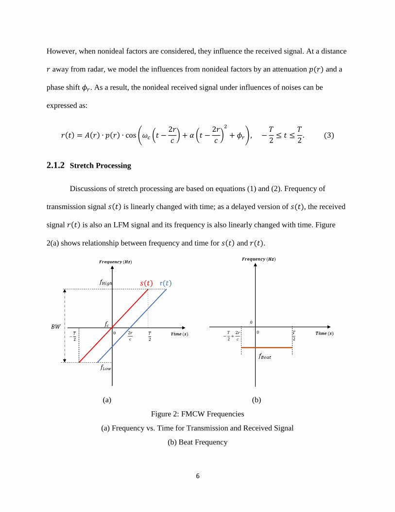
Discussions of stretch processing are based on equations (1) and (2). Frequency of
transmission signal 𝑠(𝑡) is linearly changed with time; as a delayed version of 𝑠(𝑡), the received
signal 𝑟(𝑡) is also an LFM signal and its frequency is also linearly changed with time. Figure
2(a) shows relationship between frequency and time for 𝑠(𝑡) and 𝑟(𝑡).
(a) (b)
Figure 2: FMCW Frequencies
(a) Frequency vs. Time for Transmission and Received Signal
(b) Beat Frequency
7
The instantaneous frequency of a cosine signal can be calculated by taking the derivative of its
argument respect to time. Because signals 𝑠(𝑡) and 𝑟(𝑡) are cosine signals, their frequencies can
be gained as follows:
𝑓𝑇𝑋(𝑡) =𝑑(arg (𝑠(𝑡)))
𝑑𝑡=𝑑((2𝜋𝑓𝑐+𝛼𝑡)∙𝑡)
𝑑𝑡= 2𝜋𝑓𝑐 + 2𝛼𝑡, −
𝑇
2≤ 𝑡 ≤
𝑇
2 (4)
𝑓𝑅𝑋(𝑡) =𝑑(arg (𝑟(𝑡)))
𝑑𝑡=𝑑(2𝜋𝑓𝑐(𝑡−
2𝑟
𝑐)+𝛼(𝑡−
2𝑟
𝑐)2)
𝑑𝑡= 2𝜋𝑓𝑐 + 2𝛼(𝑡 −
2𝑟
𝑐) , −
𝑇
2≤ 𝑡 ≤
𝑇
2 (5)
where 𝑓𝑇𝑋(𝑡) is the frequency of transmission signal and 𝑓𝑅𝑋(𝑡) is the frequency of received
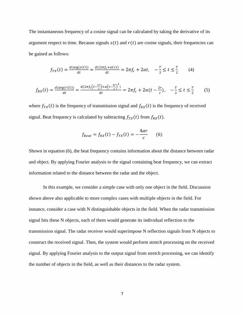
signal. Beat frequency is calculated by subtracting 𝑓𝑇𝑋(𝑡) from 𝑓𝑅𝑋(𝑡).
𝑓𝐵𝑒𝑎𝑡 = 𝑓𝑅𝑋(𝑡) − 𝑓𝑇𝑋(𝑡) = −4𝛼𝑟
𝑐 (6)
Shown in equation (6), the beat frequency contains information about the distance between radar
and object. By applying Fourier analysis to the signal containing beat frequency, we can extract
information related to the distance between the radar and the object.
In this example, we consider a simple case with only one object in the field. Discussion
shown above also applicable to more complex cases with multiple objects in the field. For
instance, consider a case with N distinguishable objects in the field. When the radar transmission
signal hits these N objects, each of them would generate its individual reflection to the
transmission signal. The radar receiver would superimpose N reflection signals from N objects to
construct the received signal. Then, the system would perform stretch processing on the received
signal. By applying Fourier analysis to the output signal from stretch processing, we can identify
the number of objects in the field, as well as their distances to the radar system.
8
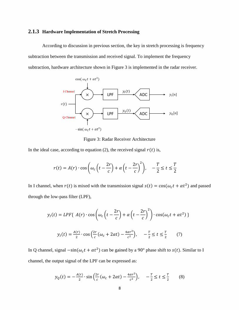
2.1.3 Hardware Implementation of Stretch Processing
According to discussion in previous section, the key in stretch processing is frequency
subtraction between the transmission and received signal. To implement the frequency
subtraction, hardware architecture shown in Figure 3 is implemented in the radar receiver.
In the ideal case, according to equation (2), the received signal 𝑟(𝑡) is,
𝑟(𝑡) = 𝐴(𝑟) ∙ cos (𝜔𝑐 (𝑡 −2𝑟
𝑐) + 𝛼 (𝑡 −
2𝑟
𝑐)2
), −𝑇
2≤ 𝑡 ≤
𝑇
2
In I channel, when 𝑟(𝑡) is mixed with the transmission signal 𝑠(𝑡) = cos (𝜔𝑐𝑡 + 𝛼𝑡2) and passed
through the low-pass filter (LPF),
𝑦𝐼(𝑡) = 𝐿𝑃𝐹 𝐴(𝑟) ∙ cos (𝜔𝑐 (𝑡 −2𝑟
𝑐) + 𝛼 (𝑡 −
2𝑟
𝑐)2
) ∙ cos(𝜔𝑐𝑡 + 𝛼𝑡2)
𝑦𝐼(𝑡) =𝐴(𝑟)
2∙ cos (
2𝑟
𝑐(𝜔𝑐 + 2𝛼𝑡) −
4𝛼𝑟2
𝑐2) , −
𝑇
2≤ 𝑡 ≤
𝑇
2 (7)
In Q channel, signal −sin (𝜔𝑐𝑡 + 𝛼𝑡2) can be gained by a 90° phase shift to 𝑠(𝑡). Similar to I
channel, the output signal of the LPF can be expressed as:
𝑦𝑄(𝑡) = −𝐴(𝑟)
2∙ sin (
2𝑟
𝑐(𝜔𝑐 + 2𝛼𝑡) −
4𝛼𝑟2
𝑐2) , −
𝑇
2≤ 𝑡 ≤
𝑇
2 (8)
Figure 3: Radar Receiver Architecture
9
2.2 Backprojection Algorithm
2.2.1 Signal Model for Single Pulse
Based on signals 𝑦𝐼(𝑡) and 𝑦𝑄(𝑡) in equations (7) and (8), signal 𝑦(𝑡), referred as
“complex IQ data” can be constructed for post processing, as shown in equation (9). Complex IQ
data, 𝑦(𝑡), contains information about beat frequency mentioned above.
𝑦(𝑡) = 𝑦𝐼(𝑡) + 𝑗 ∙ 𝑦𝑄(𝑡)
𝑦(𝑡) =𝐴(𝑟)
2∙ 𝑒−𝑗
2𝑟
𝑐(𝜔𝑐+2𝛼𝑡) ∙ 𝑒
𝑗(4𝛼𝑟2
𝑐2), −
𝑇
2≤ 𝑡 ≤
𝑇
2 (9)
In equation (9), 𝑐 is the speed of light, 𝛼 is the chirp rate of the radar system and 𝑟 is the distance
between radar and an object. Because 𝑐2 ≫ 4𝛼𝑟2, the exponential term 𝑒𝑗(4𝛼𝑟2
𝑐2) can be ignored.
Equation (9) can be simplified as:
𝑦(𝑡) =𝐴(𝑟)
2∙ 𝑒−𝑗
2𝑟
𝑐(𝜔𝑐+2𝛼𝑡) , −
𝑇
2≤ 𝑡 ≤
𝑇
2 (10)
Equation (10) shows the complex IQ data corresponding to reflection from a single object at
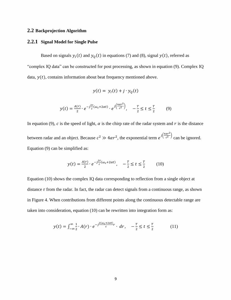
distance r from the radar. In fact, the radar can detect signals from a continuous range, as shown
in Figure 4. When contributions from different points along the continuous detectable range are
taken into consideration, equation (10) can be rewritten into integration form as:
𝑦(𝑡) = ∫1
2∙ 𝐴(𝑟) ∙ 𝑒−𝑗
2(𝜔𝑐+2𝛼𝑡)
𝑐𝑟 ∙ 𝑑𝑟
∞
−∞, −
𝑇
2≤ 𝑡 ≤
𝑇
2 (11)
10
2.2.2 Fourier Analysis
Definition of Fourier Transform and Inverse Fourier Transform are shown as follows:
𝑋(𝑗𝜔) = ∫ 𝑥(𝑡) ∙ 𝑒−𝑗𝜔𝑡 ∙ 𝑑𝑡∞
−∞ (12)
𝑥(𝑡) =1
2𝜋∫ 𝑋(𝑗𝜔) ∙ 𝑒𝑗𝜔𝑡 ∙ 𝑑𝜔∞
−∞ (13)
In equation (11), let Ω =2(𝜔𝑐+2𝛼𝑡)
𝑐 and 𝑌(𝑗Ω) = 𝑦(𝑡). Equation (11) can be written as:
𝑌(𝑗Ω) = ∫𝐴(𝑟)
2∙ 𝑒−𝑗Ω𝑟 ∙ 𝑑𝑟
∞
−∞ (14)
Comparing equation (14) with (12), observe that 𝑌(𝑗Ω) and 𝐴(𝑟)
2 satisfy the Fourier Transform
relationship. Therefore, by taking Inverse Fourier Transform (IFT) to 𝑦(𝑡), which is equivalent
to 𝑌(𝑗Ω), range profile 𝐴(𝑟) can be calculated.
Figure 4: Radar Detectable Range
11
2.2.3 Discrete-Time Signal Model for Single Pulse
In order to use a computer to perform data processing, continuous-time data from radar
receiver needs to be converted into discrete-time data. As shown in Figure 3, analog-to-digital
converters (ADC) in the radar receiver construct discrete-time signals, 𝑦𝐼[𝑛] and 𝑦𝑄[𝑛], by
sampling continuous-time signals 𝑦𝐼(𝑡) and 𝑦𝑄(𝑡). Based on 𝑦𝐼[𝑛] and 𝑦𝑄[𝑛], discrete-time
complex IQ data is constructed as:
𝑦[𝑛] = 𝑦𝐼[𝑛] + 𝑗 ∙ 𝑦𝑄[𝑛]
Equivalently, 𝑦[𝑛] can be treated as a set of samples from continuous-time complex IQ data
𝑦(𝑡).
Discrete-time complex signal 𝑦[𝑛] is constructed by taking K equal-space samples from
𝑦(𝑡). Taking samples from 𝑦(𝑡) only influences terms related to time, 𝑡. Therefore, in equation
(10), the only term influenced by sampling is (𝜔𝑐 + 2𝛼𝑡). Refer to equation (4), (𝜔𝑐 + 2𝛼𝑡) is
the instantaneous frequency of the transmission signal 𝑠(𝑡). As shown in Figure 2, the frequency
of 𝑠(𝑡) is linearly increased with time. By taking K equal-space samples from 𝑦(𝑡), following
relationship is satisfied:
(𝜔𝑐 + 2𝛼𝑡) , −𝑇
2≤ 𝑡 ≤
𝑇
2 𝑇𝑎𝑘𝑒 𝐾 𝐸𝑞𝑢𝑎𝑙−𝑆𝑝𝑎𝑐𝑒 𝑆𝑎𝑚𝑝𝑙𝑒𝑠→ 2𝜋𝑓𝐿𝑜𝑤 + 2𝜋(𝑛 − 1) ∙ ∆𝑓 , 𝑛 = 1,2, … , 𝐾 (15)
where 𝑓𝐿𝑜𝑤 denotes the minimum frequency in a pulse (unit of 𝑓𝐿𝑜𝑤 is Hz), ∆𝑓 denotes the step
frequency. Relationships among the number of samples, K, the bandwidth of the radar system,
BW, step frequency ∆𝑓 and carrier frequency 𝜔𝑐 are:
∆𝑓 =𝐵𝑊
(𝐾−1) (16)
12
𝑓𝐿𝑜𝑤 =𝜔𝑐
2𝜋−𝐵𝑊
2 (17)
By substituting the result from equation (15) into equation (10), the discrete-time complex IQ
data are:
𝑦[𝑛] =𝐴(𝑟)
2∙ 𝑒−𝑗
4𝜋𝑟∙𝑓𝐿𝑜𝑤𝑐 ∙ 𝑒−𝑗2𝜋
2𝑟∙∆𝑓
𝑐(𝑛−1), 𝑛 = 1,2,3, … , 𝐾. (18)
According to analysis in Section 1.2.2, by taking IFT of the signal 𝑦(𝑡), information
about the range profile 𝐴(𝑟) is extracted. 𝑦[𝑛] in equation (18) is a discrete-time signal sampled
from 𝑦(𝑡). In order to extract information about the range profile from 𝑦[𝑛], an Inverse Discrete
Fourier Transform (IDFT) is applied to 𝑦[𝑛]. Let 𝐴[𝑚] denote the set of equal-space samples of
range profile, 𝐴(𝑟), in the spatial domain. 𝐴[𝑚] is called “discrete-time range profile.” The
argument, 𝑚, represents the index. The relationship between 𝐴(𝑟) and 𝐴[𝑚] is:
𝐴[𝑚] =𝐴(𝑟)
2 |𝑟=
𝑚−1
𝐾∙𝑊𝑟 , 𝑚 = 1,2,3, … , 𝐾 (19)
where, 𝑊𝑟 represents the maximum alias-free range extent of the image from radar system.
Information about 𝑊𝑟 is discussed in section 2.24.
When parameter 𝑟 in equation (18) is written as (𝑚−1
𝐾∙ 𝑊𝑟), equation (18) becomes:
𝑦[𝑛] = 𝐴[𝑚] ∙ 𝑒−𝑗4𝜋𝑟∙𝑓𝐿𝑜𝑤
𝑐 ∙ 𝑒−𝑗2𝜋2∙(𝑚−1)∙𝑊𝑟∙∆𝑓
𝐾∙𝑐(𝑛−1), 𝑛 = 1,2,3, … , 𝐾; 𝑚 = 1,2,3, … , 𝐾. (20)
Particularly, we keep parameter 𝑟 in 𝑒−𝑗4𝜋𝑟∙𝑓𝐿𝑜𝑤
𝑐 in equation (20), for the convenience in next-
stage analysis.
13
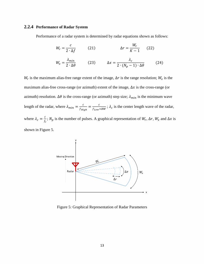
2.2.4 Performance of Radar System
Performance of a radar system is determined by radar equations shown as follows:
𝑊𝑟 =𝑐
2 ∙ ∆𝑓 (21) ∆𝑟 =
𝑊𝑟𝐾 − 1
(22)
𝑊𝑥 =𝜆𝑚𝑖𝑛2 ∙ ∆𝜃
(23) ∆𝑥 =𝜆𝑐
2 ∙ (𝑁𝑝 − 1) ∙ ∆𝜃 (24)
𝑊𝑟 is the maximum alias-free range extent of the image, ∆𝑟 is the range resolution; 𝑊𝑥 is the
maximum alias-free cross-range (or azimuth) extent of the image, ∆𝑥 is the cross-range (or
azimuth) resolution. ∆𝜃 is the cross-range (or azimuth) step size; 𝜆𝑚𝑖𝑛 is the minimum wave
length of the radar, where 𝜆𝑚𝑖𝑛 =𝑐
𝑓𝐻𝑖𝑔ℎ=
𝑐
𝑓𝐿𝑜𝑤+𝐵𝑊 ; 𝜆𝑐 is the center length wave of the radar,
where 𝜆𝑐 =𝑐
𝑓𝑐; 𝑁𝑝 is the number of pulses. A graphical representation of 𝑊𝑟, ∆𝑟, 𝑊𝑥 and ∆𝑥 is
shown in Figure 5.
Figure 5: Graphical Representation of Radar Parameters
14
2.2.5 Range Profile for Single Pulse
The analysis in Section 2.2.3 shows that information about range profile, 𝐴(𝑟), can be
extracted by taking IDFT of 𝑦[𝑛] in equation (20). In MATLAB, the IDFT of a signal 𝑋 is
finished by calling function 𝑖𝑓𝑓𝑡(𝑋). The definition of function 𝑖𝑓𝑓𝑡(𝑋) is: [10]
𝑥(𝑚) =1
𝐾∑ 𝑋(𝑛) ∙ 𝑒𝑗∙
2𝜋
𝐾(𝑚−1)(𝑛−1)𝐾
𝑛=1 (25)
where K is the number of samples.
Applying function 𝑖𝑓𝑓𝑡 to signal 𝑦[𝑛] in equation (20), the result is shown as follows:
𝑖𝑓𝑓𝑡( 𝑦[𝑛]) = 1
𝐾∑ 𝑦[𝑛] ∙ 𝑒𝑗∙
2𝜋
𝐾(𝑚−1)(𝑛−1)𝐾
𝑛=1
𝑖𝑓𝑓𝑡( 𝑦[𝑛]) =1
𝐾∑(𝐴[𝑚] ∙ 𝑒−𝑗
4𝜋𝑟∙𝑓𝐿𝑜𝑤𝑐 ∙ 𝑒−𝑗2𝜋
2∙(𝑚−1)∙𝑊𝑟∙∆𝑓𝐾∙𝑐
(𝑛−1)) ∙ 𝑒𝑗∙2𝜋𝐾(𝑚−1)(𝑛−1)
𝐾
𝑛=1
𝑖𝑓𝑓𝑡(𝑦[𝑛]) =1
𝐾∑ 𝐴[𝑚] ∙ 𝑒−𝑗
4𝜋𝑟∙𝑓𝐿𝑜𝑤𝑐 ∙ 𝑒𝑗2𝜋
(𝑛−1)(𝑚−1
𝐾 −
2∙(𝑚−1)∙𝑊𝑟∙∆𝑓
𝐾∙𝑐)𝐾
𝑛=1 . (26)
Combining equation (21), 𝑊𝑟 =𝑐
2∙∆𝑓 , and equation (26) yields:
𝑃[𝑚] = 𝑖𝑓𝑓𝑡(𝑦[𝑛]) =1
𝐾∙ 𝐴[𝑚] ∙ 𝑒−𝑗
4𝜋𝑟∙𝑓𝐿𝑜𝑤𝑐 ∑𝑒𝑗2𝜋(𝑛−1)×0
𝐾
𝑛=1
𝑃[𝑚] = 𝑖𝑓𝑓𝑡(𝑦[𝑛]) = 𝐴[𝑚] ∙ 𝑒−𝑗4𝜋𝑟∙𝑓𝐿𝑜𝑤
𝑐 (27)
𝑃[𝑚] is the discrete-time range profile of a pulse without phase correction and it is called “pre-
correction range profile.” By multiplying phase correction term 𝑒𝑗4𝜋𝑟∙𝑓𝐿𝑜𝑤
𝑐 on both sides of
equation (27), it becomes:
15
𝐴[𝑚] = 𝑒𝑗4𝜋𝑟∙𝑓𝐿𝑜𝑤
𝑐 ∙ 𝑃[𝑚] (28)
where 𝐴[𝑚] is the discrete-time range profile of a pulse. In equation (28), samples m indexes the
range according to:
𝑟 =𝑚−1
𝐾∙ 𝑊𝑟 𝑚 = 1,2,3, … , 𝐾. (29)
Equation (29) maps the sample index to physical distance between the object and radar.
Alternatively, shown in equation (30), application of the 𝑓𝑓𝑡𝑠ℎ𝑖𝑓𝑡() command in
MATLAB to equation (29) reorganizes the signal and puts 𝑚 = 1 at the center of the range
profile. The mapping between the index and physical distance is given by equation (31).
𝐴[𝑚] = 𝑒𝑗4𝜋𝑟∙𝑓𝐿𝑜𝑤
𝑐 ∙ 𝑓𝑓𝑡𝑠ℎ𝑖𝑓𝑡 𝑖𝑓𝑓𝑡(𝑦[𝑛]) = 𝑒𝑗4𝜋𝑟∙𝑓𝐿𝑜𝑤
𝑐 ∙ 𝑓𝑓𝑡𝑠ℎ𝑖𝑓𝑡 𝑃[𝑚] (30)
𝑟 =𝑚−1
𝐾∙ 𝑊𝑟 𝑚 = −
𝐾
2, (1 −
𝐾
2) , … , (
𝐾
2− 1). (31)
By combing equations (19), (28) and (29) (or equations (19), (30) and (31)), the range
profile, 𝐴(𝑟) can be computed.
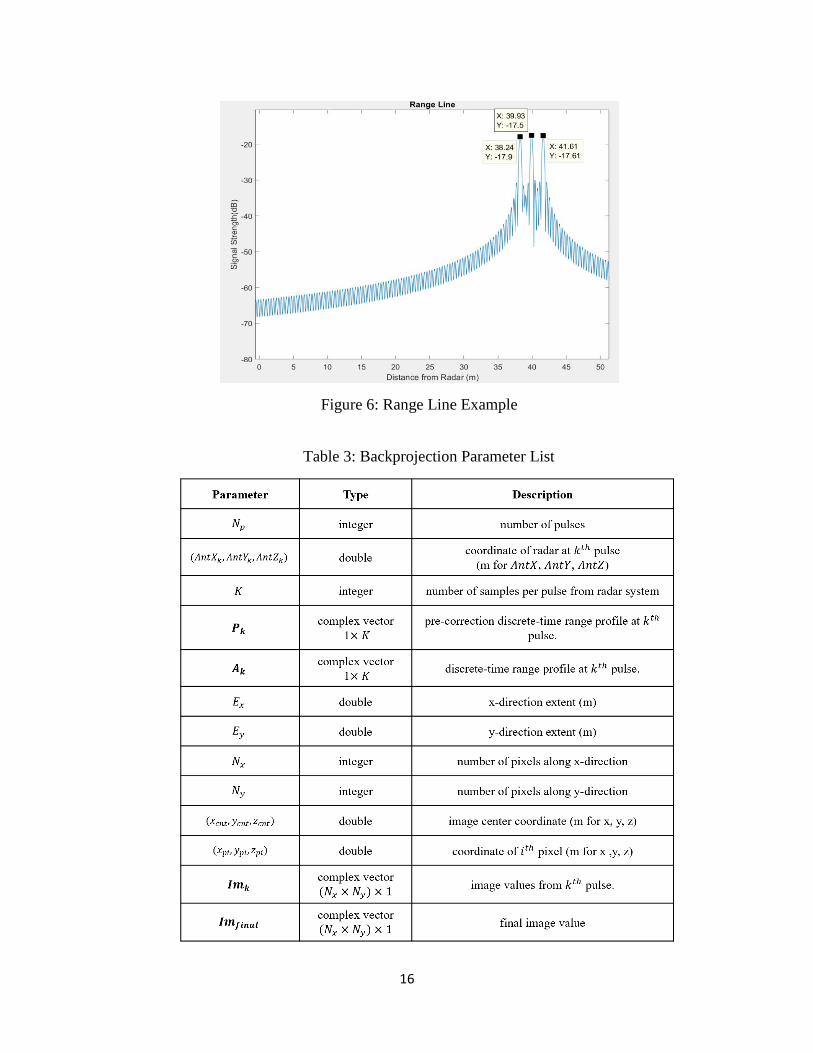
“Range line” is a figure describing the relationship between the distance, 𝑟 and the
magnitude of range profile |𝐴(𝑟)|. A range line shows information about objects in the detected
field. Figure 6 is an example showing the range line for one pulse. Three peaks in Figure 6
correspond to three distinguishable objects in the field; distances from the radar system to three
objects are 38.24m, 39.93m and 41.61m.
16
Figure 6: Range Line Example
Table 3: Backprojection Parameter List
17
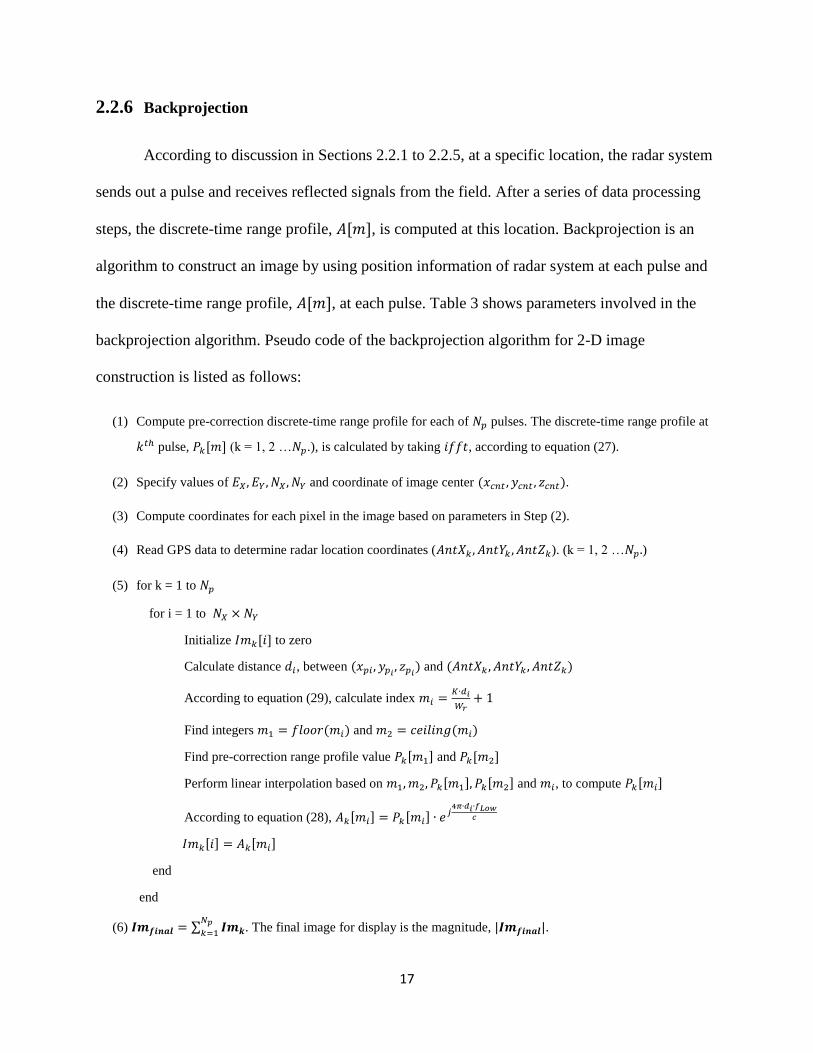
2.2.6 Backprojection
According to discussion in Sections 2.2.1 to 2.2.5, at a specific location, the radar system
sends out a pulse and receives reflected signals from the field. After a series of data processing
steps, the discrete-time range profile, 𝐴[𝑚], is computed at this location. Backprojection is an
algorithm to construct an image by using position information of radar system at each pulse and
the discrete-time range profile, 𝐴[𝑚], at each pulse. Table 3 shows parameters involved in the
backprojection algorithm. Pseudo code of the backprojection algorithm for 2-D image
construction is listed as follows:
(1) Compute pre-correction discrete-time range profile for each of 𝑁𝑝 pulses. The discrete-time range profile at
𝑘𝑡ℎ pulse, 𝑃𝑘[𝑚] (k = 1, 2 …𝑁𝑝.), is calculated by taking 𝑖𝑓𝑓𝑡, according to equation (27).
(2) Specify values of 𝐸𝑋, 𝐸𝑌 , 𝑁𝑋, 𝑁𝑌 and coordinate of image center (𝑥𝑐𝑛𝑡 , 𝑦𝑐𝑛𝑡 , 𝑧𝑐𝑛𝑡).
(3) Compute coordinates for each pixel in the image based on parameters in Step (2).
(4) Read GPS data to determine radar location coordinates (𝐴𝑛𝑡𝑋𝑘 , 𝐴𝑛𝑡𝑌𝑘 , 𝐴𝑛𝑡𝑍𝑘). (k = 1, 2 …𝑁𝑝.)
(5) for k = 1 to 𝑁𝑝
for i = 1 to 𝑁𝑋 × 𝑁𝑌
Initialize 𝐼𝑚𝑘[𝑖] to zero
Calculate distance 𝑑𝑖, between (𝑥𝑝𝑖 , 𝑦𝑝𝑖 , 𝑧𝑝𝑖) and (𝐴𝑛𝑡𝑋𝑘 , 𝐴𝑛𝑡𝑌𝑘 , 𝐴𝑛𝑡𝑍𝑘)
According to equation (29), calculate index 𝑚𝑖 =𝐾∙𝑑𝑖
𝑊𝑟+ 1
Find integers 𝑚1 = 𝑓𝑙𝑜𝑜𝑟(𝑚𝑖) and 𝑚2 = 𝑐𝑒𝑖𝑙𝑖𝑛𝑔(𝑚𝑖)
Find pre-correction range profile value 𝑃𝑘[𝑚1] and 𝑃𝑘[𝑚2]
Perform linear interpolation based on 𝑚1, 𝑚2, 𝑃𝑘[𝑚1], 𝑃𝑘[𝑚2] and 𝑚𝑖, to compute 𝑃𝑘[𝑚𝑖]
According to equation (28), 𝐴𝑘[𝑚𝑖] = 𝑃𝑘[𝑚𝑖] ∙ 𝑒𝑗4𝜋∙𝑑𝑖∙𝑓𝐿𝑜𝑤
𝑐
𝐼𝑚𝑘[𝑖] = 𝐴𝑘[𝑚𝑖]
end
end
(6) 𝑰𝒎𝒇𝒊𝒏𝒂𝒍 = ∑ 𝑰𝒎𝒌𝑁𝑝𝑘=1 . The final image for display is the magnitude, |𝑰𝒎𝒇𝒊𝒏𝒂𝒍|.
18
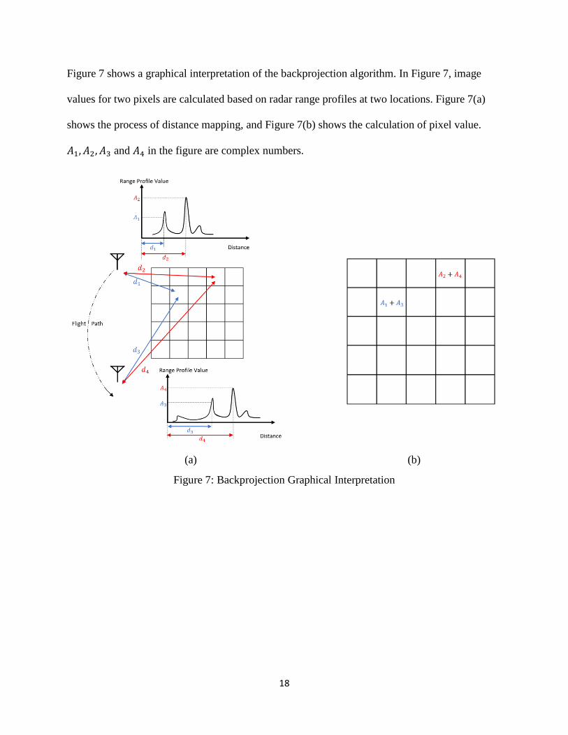
Figure 7 shows a graphical interpretation of the backprojection algorithm. In Figure 7, image
values for two pixels are calculated based on radar range profiles at two locations. Figure 7(a)
shows the process of distance mapping, and Figure 7(b) shows the calculation of pixel value.
𝐴1, 𝐴2, 𝐴3 and 𝐴4 in the figure are complex numbers.
(a) (b)
Figure 7: Backprojection Graphical Interpretation
19
CHAPTER 3: Autofocus Algorithm
Measurement in SAR system is sensitive to non-ideal factors, such as environmental
noises, atmospheric propagation delays in the radar signal, etc. These non-ideal factors smear or
blur the SAR image. In order to construct a high-quality SAR image without extra hardware cost,
an autofocus algorithm is necessary. In 2012, Joshua N. Ash proposed a SAR autofocus method
based on backprojection imaging [8]. The goal of the autofocus method is to maximize the
sharpness of the SAR image.
3.1 General Signal Model
The sharpness of the image is defined as:
𝑠() =∑𝛹(𝑣𝑚())
𝑚
where 𝑣𝑚() is the intensity of the 𝑚𝑡ℎ pixel in the image after a set of phase corrections, and
𝛹(𝑥) is a convex function. 𝛹(𝑥) = 𝑥2 is a reasonable choice in the algorithm, because it not
only provides a closed-form solution for the final result, but also yields maximum likelihood
phase error estimation for the model in [8]. Therefore, the sharpness of the SAR image can be
determined as:
𝑠() = ∑ (𝑣𝑚())2
𝑚 = || 𝒗 ||2 (32)
According to Section 2.2.6, a SAR image can be represented as:
𝑰𝒎𝒇𝒊𝒏𝒂𝒍 = ∑ 𝑰𝒎𝒌𝑁𝑝𝑘=1 (33)
where the meaning of parameters 𝑁𝑝, 𝑰𝒎𝒌 and 𝑰𝒎𝒇𝒊𝒏𝒂𝒍 are defined in Table 3.
20
Two assumptions are made in this autofocus algorithm:
1) Influences from non-ideal factors can be modeled as a phase error per pulse:
𝑰𝒌 = 𝑰𝒎𝒌 ∙ 𝑒𝑗𝜙𝑘 (34)
where 𝑰𝒎𝒌 denotes the uncorrupted image value at the 𝑘𝑡ℎ pulse, 𝑰𝒎 denotes the
corrupted image value at the 𝑘𝑡ℎ pulse and 𝜙𝑘 denotes the phase error at the 𝑘𝑡ℎ pulse.
2) For different values of 𝑘, the values of 𝜙𝑘 are independent of each other.
The goal of the algorithm is to find a set of optimal phase corrections, = 1, 2, … , 𝑁𝑝, so
that the sharpness of
𝑰𝒇𝒊𝒏𝒂𝒍 = ∑ 𝑰𝒌𝑁𝑝𝑘=1 ∙ 𝑒−𝑗𝑘 (35)
is maximized under the metric shown in equation (32). The optimal phase correction is denoted
as:
= arg max𝜙(𝑠(𝜙)) . (36)
According to assumption 2) mentioned above, because the values of 𝜙𝑘 are independent of each
other for different values of 𝑘, each parameter in the set can be optimized in turn, while the
rest of parameters are kept unchanged. Optimization over the set can be performed for
multiple iterations. We denote the optimal phase correction for the 𝑘𝑡ℎ pulse in the 𝑖𝑡ℎ iteration
as 𝑘𝑖 . The optimal phase correction for the 𝑘𝑡ℎ pulse in the (𝑖 + 1)𝑡ℎ iteration can be
represented as:
𝑘𝑖+1 = arg max
𝜙( 𝑠(1
𝑖+1, 2𝑖+1, … , 𝜙, 𝑘+1
𝑖 , … , 𝑁𝑝𝑖 ) ) , 𝑘 = 1,2, … ,𝑁𝑝. (37)
21
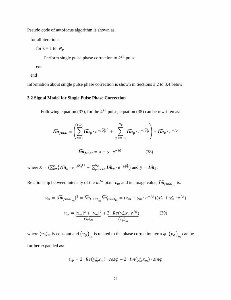
Pseudo code of autofocus algorithm is shown as:
Information about single pulse phase correction is shown in Sections 3.2 to 3.4 below.
3.2 Signal Model for Single Pulse Phase Correction
Following equation (37), for the 𝑘𝑡ℎ pulse, equation (35) can be rewritten as:
𝑰𝒇𝒊𝒏𝒂𝒍 = (∑𝑰𝒑
𝑘−1
𝑝=1
∙ 𝑒−𝑗𝑝𝑖+1+ ∑ 𝑰𝒑
𝑁𝑝
𝑝=𝑘+1
∙ 𝑒−𝑗𝑝𝑖) + 𝑰𝒌 ∙ 𝑒
−𝑗𝜙
𝑰𝒇𝒊𝒏𝒂𝒍 = 𝒙 + 𝒚 ∙ 𝑒−𝑗𝜙 (38)
where 𝒙 = (∑ 𝑰𝒑𝑘−1𝑝=1 ∙ 𝑒−𝑗𝑝
𝑖+1+ ∑ 𝑰𝒑
𝑁𝑝𝑝=𝑘+1 ∙ 𝑒−𝑗𝑝
𝑖) and 𝒚 = 𝑰𝒌.
Relationship between intensity of the 𝑚𝑡ℎ pixel 𝑣𝑚 and its image value, 𝐼𝑓𝑖𝑛𝑎𝑙𝑚 is:
𝑣𝑚 = |𝐼𝑓𝑖𝑛𝑎𝑙𝑚|2 = 𝐼𝑓𝑖𝑛𝑎𝑙𝑚
𝐼𝑓𝑖𝑛𝑎𝑙𝑚∗ = (𝑥𝑚 + 𝑦𝑚 ∙ 𝑒
−𝑗𝜙)(𝑥𝑚∗ + 𝑦𝑚
∗ ∙ 𝑒𝑗𝜙)
𝑣𝑚 = |𝑥𝑚|2 + |𝑦𝑚|
2⏟ (𝑣0)𝑚
+ 2 ∙ 𝑅𝑒(𝑦𝑚∗ 𝑥𝑚𝑒
𝑗𝜙)⏟ (𝑣𝜙)𝑚
(39)
where (𝑣0)𝑚 is constant and (𝑣𝜙)𝑚 is related to the phase correction term 𝜙. (𝑣𝜙)𝑚
can be
further expanded as:
𝑣𝜙 = 2 ∙ 𝑅𝑒(𝑦𝑚∗ 𝑥𝑚) ∙ 𝑐𝑜𝑠𝜙 − 2 ∙ 𝐼𝑚(𝑦𝑚
∗ 𝑥𝑚) ∙ 𝑠𝑖𝑛𝜙
for all iterations
for k = 1 to 𝑁𝑝
Perform single pulse phase correction to 𝑘𝑡ℎ pulse
end
end
22
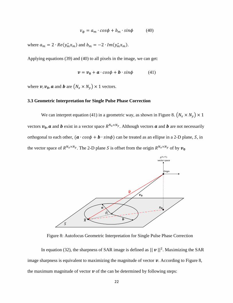
𝑣𝜙 = 𝑎𝑚 ∙ 𝑐𝑜𝑠𝜙 + 𝑏𝑚 ∙ 𝑠𝑖𝑛𝜙 (40)
where 𝑎𝑚 = 2 ∙ 𝑅𝑒(𝑦𝑚∗ 𝑥𝑚) and 𝑏𝑚 = −2 ∙ 𝐼𝑚(𝑦𝑚
∗ 𝑥𝑚).
Applying equations (39) and (40) to all pixels in the image, we can get:
𝒗 = 𝒗𝟎 + 𝒂 ∙ 𝑐𝑜𝑠𝜙 + 𝒃 ∙ 𝑠𝑖𝑛𝜙 (41)
where 𝒗, 𝒗𝟎, 𝒂 and 𝒃 are (𝑁𝑥 × 𝑁𝑦) × 1 vectors.
3.3 Geometric Interpretation for Single Pulse Phase Correction
We can interpret equation (41) in a geometric way, as shown in Figure 8. (𝑁𝑥 × 𝑁𝑦) × 1
vectors 𝒗𝟎, 𝒂 and 𝒃 exist in a vector space 𝑅𝑁𝑥×𝑁𝑦. Although vectors 𝒂 and 𝒃 are not necessarily
orthogonal to each other, (𝒂 ∙ 𝑐𝑜𝑠𝜙 + 𝒃 ∙ 𝑠𝑖𝑛𝜙) can be treated as an ellipse in a 2-D plane, 𝑆, in
the vector space of 𝑅𝑁𝑥×𝑁𝑦. The 2-D plane 𝑆 is offset from the origin 𝑅𝑁𝑥×𝑁𝑦 of by 𝒗𝟎
In equation (32), the sharpness of SAR image is defined as || 𝒗 ||2. Maximizing the SAR
image sharpness is equivalent to maximizing the magnitude of vector 𝒗. According to Figure 8,
the maximum magnitude of vector 𝒗 of the can be determined by following steps:
Figure 8: Autofocus Geometric Interpretation for Single Pulse Phase Correction

23
① Project the origin of 𝑅𝑁𝑥×𝑁𝑦 into 2-D plane 𝑆. Denote the projection point as 𝒙𝟎.
② Find the optimal focus point on the eclipse, which is farthest away from 𝒙𝟎.
③ Determined the optimal phase correction factor corresponding to .
④ Substitute for 𝜙 in equation (38) to complete single pulse phase correction.
3.4 Phase Optimization for Single Pulse Phase Correction
In this section, we will provide detailed information about the 4-step process mentioned
in Section 3.3, which maximizes the sharpness of an image from SAR system. According to
Figure 8, the 2-D plane S in vector space of 𝑅𝑁𝑥×𝑁𝑦 is defined by vectors 𝒂 and 𝒃. By
performing orthogonalization of 𝒂 and 𝒃, we get a basis 𝒆𝟏, 𝒆𝟐 for the S plane:
𝐞𝟏 =𝒂
||𝒂|| 𝐞𝟐 =
𝒃−𝒆𝟏𝒆𝟏𝑻𝒃
||𝒃−𝒆𝟏𝒆𝟏𝑻𝒃||
. (42)
In the S plane, 𝒂 and 𝒃 become
≡ [12] = 𝑬𝑻𝒂 ≡ [
12] = 𝑬𝑻𝒃 (43)
where 𝐄 = [𝐞𝟏 𝐞𝟐]. In the original vector space 𝑅𝑁𝑥×𝑁𝑦, the origin in S plane is offset by
vector 𝒗𝟎. In a relative perspective, in S plane, the origin of vector space 𝑅𝑁𝑥×𝑁𝑦 is offset from S
plane origin by vector −𝒗𝟎. The projection point of the vector space origin in S plane is 𝒙𝟎,
determined by:
𝒙𝟎 = 𝑬𝑻(𝑬𝑬𝑻)(−𝒗𝟎) = −𝑬
𝑻𝒗𝟎. (44)
For a point 𝒙 on the ellipse in the S plane, we denote the normal at this point as 𝒏(𝒙). For the
optimal focus point on the ellipse, the vector 𝒙𝟎 − is parallel to the normal at , 𝒏(). This
relationship between the vector 𝒙𝟎 − and 𝒏() can be represented as:
24
𝒙𝟎 − = 𝛼 𝒏() (45)
where 𝛼 is an unknown real constant. The parametric equation of the ellipse in the 𝑆 plane can be
written as:
𝑓(𝒙) ≡ 𝒙𝑻𝑹𝒙 = 1 (46)
with
𝒙 = 𝑐𝑜𝑠𝜙 + 𝑠𝑖𝑛𝜙 = [ ] × [𝑐𝑜𝑠𝜙𝑠𝑖𝑛𝜙
] (47)
𝑹 = [𝑟1 𝑟3𝑟3 𝑟2
] (48)
𝑐 = (21 − 12)2 (49)
𝑟1 =22+2
2
𝑐 (50)
𝑟2 =12+1
2
𝑐 (51)
𝑟3 = −12+12
𝑐 . (52)
Shown as follows, the normal to the ellipse can be computed by taking the gradient of its
parametric equation shown in (46):
𝒏(𝒙) ≡ ∇𝑓(𝒙) = 2𝑹𝒙. (53)
Substituting the result of equation (53) into equation (45) and combining the constant 2 from
(53) into the unknown real constant 𝛼, we can get:
𝒙𝟎 − = 𝛼 𝑹
25
= (𝛼𝑹 + 𝑰)−1 𝒙𝟎 (54)
where 𝑰 is identity matrix. Eigenvalue decomposition of the matrix 𝑹 is denoted as 𝑹 = 𝑽𝜦𝑽𝑻,
where 𝜦 = 𝑑𝑖𝑎𝑔(𝜆1, 𝜆2) and 𝜆1, 𝜆2 are eigenvalues of matrix 𝑹. Then, we have
(𝛼𝑹 + 𝑰) = (𝛼𝑽𝜦𝑽𝑻 + 𝑰) = 𝑽(𝛼𝜦 + 𝑰)𝑽𝑻. (55)
Because is a point on the ellipse defined by equation (47), we can substitute to yield:
𝑻𝑹 = 1. (56)
Substituting equations (55) and (54) into equation (56), we obtain:
1 = 𝒙𝟎𝑻 (𝛼𝑹 + 𝑰)−1 𝑹 (𝛼𝑹 + 𝑰)−1 𝒙𝟎
1 = 𝒙𝟎𝑻 𝑽(𝛼𝜦 + 𝑰)−1𝑽𝑻𝑹 𝑽(𝛼𝜦 + 𝑰)−1𝑽𝑻 𝒙𝟎
1 = 𝒙𝟎𝑻 𝑽(𝛼𝜦 + 𝑰)−1𝑽𝑻𝑽𝜦𝑽𝑻 𝑽(𝛼𝜦 + 𝑰)−1𝑽𝑻 𝒙𝟎
1 = 𝒙𝟎𝑻 𝑽(𝛼𝜦 + 𝑰)−1𝜦 (𝛼𝜦 + 𝑰)−1𝑽𝑻 𝒙𝟎
1 = 𝒙𝟎𝑻 𝑽 [
𝜆1
(𝛼𝜆1+1)20
0𝜆2
(𝛼𝜆2+1)2
] 𝑽𝑻 𝒙𝟎 (57)
Let [𝛽1, 𝛽2]𝑇 = 𝑽𝑻 𝒙𝟎 ; then, equation (57) can be written as:
𝛽12
𝜆1
(𝛼𝜆1+1)2+ 𝛽2
2 𝜆2
(𝛼𝜆2+1)2− 1 = 0 (58)
The roots of equation (58) are the same as the roots of the forth-order polynomial in equation
(59) [11].
𝑔(𝛼) = ∑ 𝛾𝑚 𝛼𝑚4
𝑚=0 (59)
26
where
𝛾0 = 𝜆1𝛽12 + 𝜆2𝛽2
2 − 1 (60)
𝛾1 = 2𝜆1(𝜆2𝛽22 − 1) + 2𝜆2(𝜆1𝛽1
2 − 1) (61)
𝛾2 = (𝜆1𝛽12 − 1)𝜆2
2 + (𝜆2𝛽22 − 1)𝜆1
2 − 4𝜆1𝜆2 (62)
𝛾3 = −2𝜆1𝜆2(𝜆1 + 𝜆2) (63)
𝛾4 = −(𝜆1𝜆2)2. (64)
Among the four roots of the fourth-order polynomial in equation (59), the smallest real root
corresponds to the farthest distance on the eclipse to the point 𝒙𝟎 in the 𝑆 plane [11]. According
to the requirement from Step ② in Section 3.3, we pick up the smallest real root of the
polynomial in equation (59) and denote it as . Then, we substitute for 𝛼 in equation (54) to
get:
= (𝑹 + 𝑰)−1 𝒙𝟎. (65)
Combining equation (47) with equation (65), we get:
[𝑐𝑜𝑠
𝑠𝑖𝑛] = [ ]
−1 (𝑹 + 𝑰)−1 𝒙𝟎 (66)
where is the optimal phase correction factor. Based on equation (66), we can get:
𝑒−𝑗𝜙 = 𝑐𝑜𝑠 − 𝑗 𝑠𝑖𝑛 (67)
By substituting equation (67) for 𝑒−𝑗𝜙 in equation (38), single pulse phase correction is
completed.
27
CHAPTER 4: Results
4.1 Software Products
Based on the discussion from Chapter 2 and 3, we implemented a data simulator and
image processing software for the SAR system. The processing flows of the data simulator and
the image processing software are shown in Figure 9.
In Figure 9(a), “Input 1” allows the user to defined the number of objects and their
locations in the field; for “Input 2,” system location information can either be user-defined or
(a)
(b)
Figure 9: Software Processing Flow
(a) Data Simulator Processing Flow (b) Image Processing Software Processing Flow
28
imported from GPS; information about “Construct Phase History” can be referred from Section
2.1; “Backprojection” in the figure implements information from Section 2.2; information about
processes “Add Phase Error” and “Autofocus” is given in Chapter 3.
In Figure 9(b), for “Input 1,” signals 𝑦𝐼[𝑛] and 𝑦𝑄[𝑛] are the same as those mentioned in
Figure 3. Position data in “Input 2” can either be imported from GPS or recorded by other
hardware devices.
“Pre-processing” in Figure 9(b) consists of two stages. Stage 1, is called “IQ data
correction.” Ideally, the phase difference between 𝑦𝐼[𝑛] and 𝑦𝑄[𝑛] is 90°, the magnitude of 𝑦𝐼[𝑛]
and 𝑦𝑄[𝑛] are the same and DC offsets for both 𝑦𝐼[𝑛] and 𝑦𝑄[𝑛] are zero. However, due to
hardware noises, the output signals 𝑦𝐼𝑜[𝑛] and 𝑦𝑄𝑜[𝑛] from the radar receiver are different from
ideal case. “IQ data correction” is a process performing adjustments to 𝑦𝐼𝑜[𝑛] and 𝑦𝑄𝑜[𝑛], such
that the output from the process, 𝑦𝐼𝑐[𝑛] and 𝑦𝑄𝑐[𝑛] hold the relationship in ideal case. Detailed
information about “IQ data correction” is illustrated in Section 5.2. In the second stage of the
“Pre-processing,” signal 𝑦𝐵𝑃[𝑛] is constructed as:
𝑦𝐵𝑃[𝑛] = (𝑦𝐼𝑐[𝑛] + 𝑗 ∙ 𝑦𝑄𝑐[𝑛]) ∙ 𝑤[𝑛] (68)
where 𝑦𝐼𝑐[𝑛] and 𝑦𝑄𝑐[𝑛] are outputs from “IQ data correction” and 𝑤[𝑛] is a windowing function
[12] to lower sidelobes. The choice of 𝑤[𝑛] is subject to hardware performance of radar system,
as well as the interference from environment.
29
4.2 Experimental Results
We conducted a series of experiments to test the performance of the SAR system. In our
experiments, we used SDR-KIT 980B Module from Ancortek Inc. as our radar. The radar
operates in X-band, with 40° horizontal antenna beam width, 20° vertical antenna beam width,
400MHz bandwidth, 9.8 GHz center frequency, and 1024 samples per sweep. For windowing
function mentioned in equation (68), we selected blackman window. Therefore, after “Pre-
Processing” in Figure 10(b), we had:
𝑦𝐵𝑃[𝑛] = (𝑦𝐼𝑐[𝑛] + 𝑗 ∙ 𝑦𝑄𝑐[𝑛]) ∙ 𝑏𝑙𝑎𝑐𝑘𝑚𝑎𝑛[𝑛] (69)
where 𝑏𝑙𝑎𝑐𝑘𝑚𝑎𝑛[𝑛] was blackman windowing function [13]. Then, we substituted 𝑦𝐵𝑃[𝑛] in
equation (69) for 𝑦[𝑛] in equation (28) or (30) for backprojection.
4.2.1 Backprojection Experiment
Shown in Figure 10(a), we setup three aluminum reflectors with different shapes and
sizes on a soccer field. We put the SAR system on an 80-cm straight rail, which provided
accurate location information. The conceptual graph in Figure 10(b) shows the relative positions
among the reflectors and the SAR system movement. By using the accurate SAR system location
information from the rail, a simulated image was constructed through backprojection, as shown
in Figure 10(c). Then, we computed an image shown in Figure 10(d) through backprojection in
the image processing software, by combining experimental data from the radar and location
information from the rail. Both simulated and experimental images consisted of 201 × 201
pixels and both of them were displayed in a 40dB dynamic range.
In the computed image, three reflectors can be clearly identified. Relative positions
among three reflectors in the computed image were similar those in the simulated image. Signal

30
strengths from the three reflectors in the simulated image were the same, while signal strengths
from the three reflectors in experimental image were different. This was reasonable, because the
simulator focused on displaying reflectors on correct positions and it ignored sizes and shapes of
reflectors, as well as signal decay associated with the distance. In reality, signal strength from a
reflector is subject to its size, its shape, and its distance from radar. The position coordinates of
three reflectors in the simulated image were (10, 1.08), (15, -0.96) and (25, 0.12), while in the
experimental image, their corresponding coordinates were (11.6, 0.24), (17, -2.34) and (27.5, -
2.1). Compared to reflectors in the simulated image, the absolute position of each reflector in the
experimental image was shifted to the right in the range direction and shifted down in the cross-
range direction.
(a) (b)
(c) (d)
Figure 10: Backprojection Experiment
(a) Physical Setup of Reflectors (b) Conceptual Graph
(c) Simulated SAR Image (d) Experimental SAR Image
31
4.2.2 Autofocus Experiment
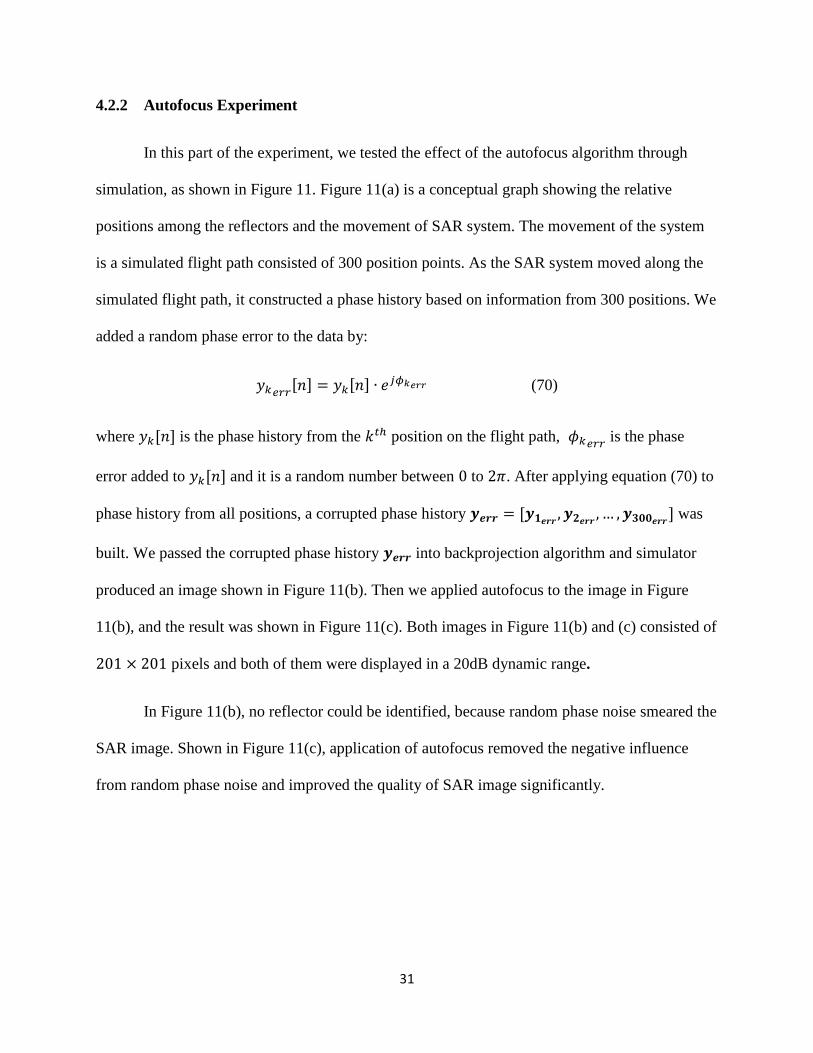
In this part of the experiment, we tested the effect of the autofocus algorithm through
simulation, as shown in Figure 11. Figure 11(a) is a conceptual graph showing the relative
positions among the reflectors and the movement of SAR system. The movement of the system
is a simulated flight path consisted of 300 position points. As the SAR system moved along the
simulated flight path, it constructed a phase history based on information from 300 positions. We
added a random phase error to the data by:
𝑦𝑘𝑒𝑟𝑟[𝑛] = 𝑦𝑘[𝑛] ∙ 𝑒𝑗𝜙𝑘𝑒𝑟𝑟 (70)
where 𝑦𝑘[𝑛] is the phase history from the 𝑘𝑡ℎ position on the flight path, 𝜙𝑘𝑒𝑟𝑟 is the phase
error added to 𝑦𝑘[𝑛] and it is a random number between 0 to 2𝜋. After applying equation (70) to
phase history from all positions, a corrupted phase history 𝒚𝒆𝒓𝒓 = [𝒚𝟏𝒆𝒓𝒓 , 𝒚𝟐𝒆𝒓𝒓 , … , 𝒚𝟑𝟎𝟎𝒆𝒓𝒓] was
built. We passed the corrupted phase history 𝒚𝒆𝒓𝒓 into backprojection algorithm and simulator
produced an image shown in Figure 11(b). Then we applied autofocus to the image in Figure
11(b), and the result was shown in Figure 11(c). Both images in Figure 11(b) and (c) consisted of
201 × 201 pixels and both of them were displayed in a 20dB dynamic range.
In Figure 11(b), no reflector could be identified, because random phase noise smeared the
SAR image. Shown in Figure 11(c), application of autofocus removed the negative influence
from random phase noise and improved the quality of SAR image significantly.
32
(a)
(b) (c)
Figure 11: Autofocus Experiment
(a) Conceptual Graph (b) Simulated SAR Image with Phase Errors
(c) Simulated SAR Image with Autofocus
Figure 12: Drone-SAR System
33
4.2.3 Drone-SAR Experiment
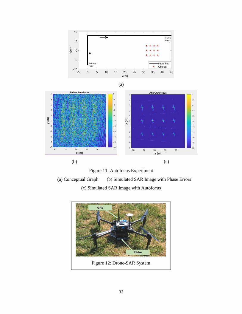
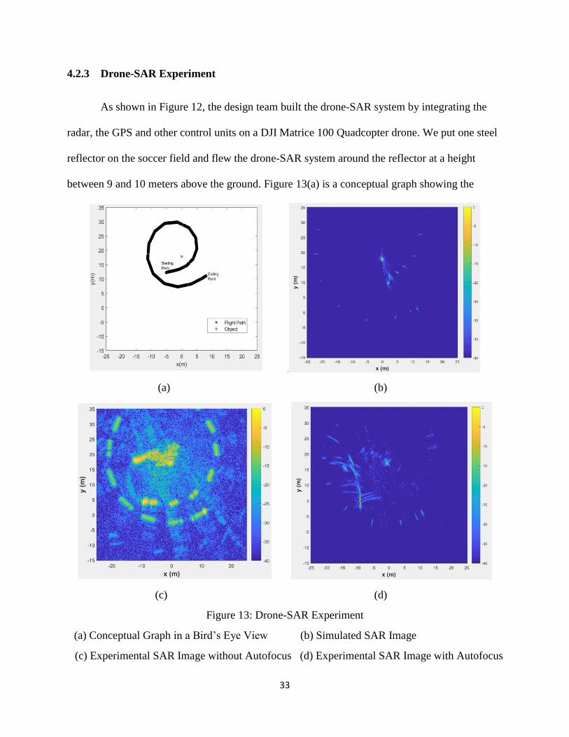
As shown in Figure 12, the design team built the drone-SAR system by integrating the
radar, the GPS and other control units on a DJI Matrice 100 Quadcopter drone. We put one steel
reflector on the soccer field and flew the drone-SAR system around the reflector at a height
between 9 and 10 meters above the ground. Figure 13(a) is a conceptual graph showing the
(a) (b)
(c) (d)
Figure 13: Drone-SAR Experiment
(a) Conceptual Graph in a Bird’s Eye View (b) Simulated SAR Image
(c) Experimental SAR Image without Autofocus (d) Experimental SAR Image with Autofocus
34
relative position between the reflector and the drone-SAR system in a bird’s eye view. By using
GPS data as location information, a simulated image was constructed, as shown in Figure 13(b).
In the image processing software, we built an image shown in Figure 13(c) by combining
experimental data from the radar and location information from the GPS. Then, we applied
autofocus to the image in Figure 13(c) and the result was shown in Figure 13(d). All images in
Figures 13(b), (c) and (d) consisted of 201 × 201 pixels and both of them were displayed in a
40dB dynamic range.
Figure 13(c) contained information in two aspects: a blurred region in the middle and a
set of rectangular artifacts. The rectangular artifacts were aliases of signals in the middle region
and the distribution of these artifacts was similar to the shape of the system flight path shown in
Figure 13(a). The region in the middle was what we were interested in, because the reflector was
included in it. During the experiment, the data from drone-SAR system was susceptible to errors.
The errors could be caused by either imperfection of hardware in drone-SAR system, or
interference from the environment. Because of the errors, in Figure 13(c), the middle region of
the SAR image was blurred and we could not identify the reflector. Autofocus made important
improvements to In Figure 13(d), after applying autofocus, although there were still remaining
artifacts in the SAR image, the reflector could be clearly identified.
35
CHAPTER 5: Error and Analysis
5.1 Ghost Peak in Near-field
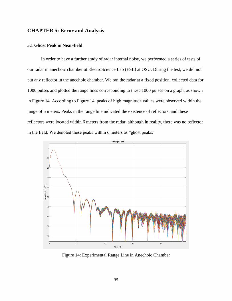
In order to have a further study of radar internal noise, we performed a series of tests of
our radar in anechoic chamber at ElectroScience Lab (ESL) at OSU. During the test, we did not
put any reflector in the anechoic chamber. We ran the radar at a fixed position, collected data for
1000 pulses and plotted the range lines corresponding to these 1000 pulses on a graph, as shown
in Figure 14. According to Figure 14, peaks of high magnitude values were observed within the
range of 6 meters. Peaks in the range line indicated the existence of reflectors, and these
reflectors were located within 6 meters from the radar, although in reality, there was no reflector
in the field. We denoted these peaks within 6 meters as “ghost peaks.”
Figure 14: Experimental Range Line in Anechoic Chamber
36
A possible cause of ghost peaks in the range line was the leakage of transmission signal. In our
radar system, the transmitting antenna and receiving antenna were close to each other. When the
transmitting antenna sent out a signal, a portion of the transmission signal went directly to the
receiving antenna within a short time delay, which likely contributed to ghost peaks in the range
line. Since ghost peaks always occurred within 6 meters from radar, in order to remove the
influence of ghost peaks on SAR image, we preprocessed the range profile data before
backprojection. Pseudo code of the preprocessing is shown as follows:
The drone-SAR experiment in Section 4.2.3 included the preprocessing mentioned above.
5.2 IQ Imbalance and IQ Correction
5.2.1 Influence of IQ Imbalance
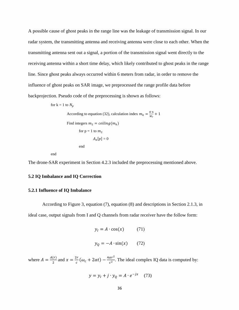
According to Figure 3, equation (7), equation (8) and descriptions in Section 2.1.3, in
ideal case, output signals from I and Q channels from radar receiver have the follow form:
𝑦𝐼 = 𝐴 ∙ cos (𝑥) (71)
𝑦𝑄 = −𝐴 ∙ sin(𝑥) (72)
where 𝐴 =𝐴(𝑟)
2 and 𝑥 =
2𝑟
𝑐(𝜔𝑐 + 2𝛼𝑡) −
4𝛼𝑟2
𝑐2. The ideal complex IQ data is computed by:
𝑦 = 𝑦𝐼 + 𝑗 ∙ 𝑦𝑄 = 𝐴 ∙ 𝑒−𝑗𝑥 (73)
for k = 1 to 𝑁𝑝
According to equation (32), calculation index 𝑚𝑘 =𝐾∙6
𝑊𝑟+ 1
Find integers 𝑚2 = 𝑐𝑒𝑖𝑙𝑖𝑛𝑔(𝑚𝑘)
for p = 1 to 𝑚2
𝐴𝑘[𝑝] = 0
end
end
37
In ideal case, signal 𝑦𝐼 and 𝑦𝑄 have the same magnitude, zero DC offset and a 90° phase
difference. However, due to errors in the radar hardware, the actual output signals from I and Q
channels are different from ideal case, and we denote this kind of phenomenon as “IQ
imbalance”. When IQ imbalance are taken into account, output signals from I and Q channels
can be modeled as:
𝑦 = 𝐴 ∙ cos(𝑥) + 𝐶 (74)
𝑦 = −𝐴𝛼 ∙ sin(𝑥 + 𝜃) + 𝐷 (75)
where 𝑦 and 𝑦 represent the corrupted I and Q signals; 𝜃 represents a phase error; 𝐶 and 𝐷
represent DC offsets in I and Q channels. Based on 𝑦 and 𝑦, the corrupted complex IQ signal
can be represented as:
= 𝑦 + 𝑗 ∙ 𝑦
= 𝐴 ∙ cos(𝑥) − 𝑗 ∙ 𝐴𝛼 ∙ 𝑐𝑜𝑠𝜃 ∙ sin(𝑥) − 𝑗 ∙ 𝐴𝛼 ∙ 𝑠𝑖𝑛𝜃 ∙ cos(𝑥) + (𝐶 + 𝑗𝐷). (76)
replace cos (𝑥) and sin (𝑥) in equation (75) with 𝑒𝑗𝑥+ 𝑒−𝑗𝑥
2 and
𝑒𝑗𝑥− 𝑒−𝑗𝑥
2, equation (76) can be
rewritten as:
= 𝐴𝑒−𝑗𝑥 ∙ [1
2+ 𝑗 ∙
𝛼
2(𝑐𝑜𝑠𝜃 − 𝑠𝑖𝑛𝜃)]⏟ 𝛽1∙𝑒𝑗𝜙1
+ 𝐴𝑒𝑗𝑥 ∙ [1
2− 𝑗 ∙
𝛼
2(𝑐𝑜𝑠𝜃 + 𝑠𝑖𝑛𝜃)]⏟ 𝛽2∙𝑒
𝑗𝜙2
+ (𝐶 + 𝑗 ∙ 𝐷)⏟ 𝛽3∙𝑒
𝑗𝜙3
= 𝐴𝑒−𝑗𝑥 ∙ 𝛽1𝑒𝑗𝜙1+ 𝐴𝑒𝑗𝑥 ∙ 𝛽2𝑒
𝑗𝜙2 + 𝛽3𝑒𝑗𝜙3. (77)
To have a further understanding to the difference between equation (73) and (77), we provide the
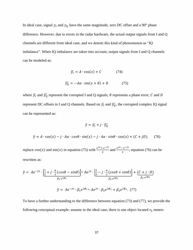
following conceptual example: assume in the ideal case, there is one object located 𝑟0 meters
38
away from the SAR system. Range lines associated with the ideal complex signal, 𝑦 and
corrupted complex signal, are plotted, as shown in Figure 15.
Two significant differences between Figure 15(a) and (b) are observed. Firstly, the peak signal
strength from the object located at 𝑟0 is attenuated by a factor of 𝛽1; Secondly, in Figure 15(b),
there are two additional peaks located at 0 and −𝑟0 meters away from the SAR system. There are
no objects in the field corresponding to these two peaks, and therefore, similar to Section 5.1, we
also denote these two peaks as “ghost peaks”. The third term, 𝛽3𝑒𝑗𝜙3, in equation (77) is the
source of the ghost peak located at 0; the second term, 𝐴𝑒𝑗𝑥 ∙ 𝛽2𝑒𝑗𝜙2 , in equation (77)
contributes to the ghost peak located at −𝑟0 meters away from the SAR system and it is the alias
Figure 15: Range Line Analysis
(a) Range Line Associated with Signal 𝑦. (b) Range Line Associated with Signal .
39
of the object located at 𝑟0. In addition, the term 𝑒𝑗𝜙1 in equation (77) brings a phase error to the
ideal reflection signal, which is not shown in Figure 15.
5.2.2 IQ Correction
Based on equation (74) and (75), the goal of IQ correction is to remove the influence of
𝐶, 𝐷, 𝛼 and 𝜃. We denote 𝑇 as the period of signal cos (𝑥) and sin (𝑥) from equations (73) and
(74). IQ correction is performed following equations (78) to (85).
𝑦𝐼𝑎𝑣𝑔 =1
𝑁∙𝑇∫ 𝑦(𝑥) 𝑑𝑥
𝑁𝑇= 𝐶 (78)
𝑦𝑄𝑎𝑣𝑔 =1
𝑁∙𝑇∫ 𝑦(𝑥) 𝑑𝑥
𝑁𝑇 = 𝐷 (79)
𝑉𝑎𝑟𝐼 =1
𝑁∙𝑇∫ (𝑦(𝑥) − 𝑦𝐼𝑎𝑣𝑔)
2
𝑑𝑥
𝑁𝑇=𝐴2
2 (80)
𝑉𝑎𝑟𝑄 =1
𝑁∙𝑇∫ (𝑦(𝑥) − 𝑦𝑄𝑎𝑣𝑔)
2
𝑑𝑥
𝑁𝑇=𝐴2𝛼2
2 (81)
𝐶𝑜𝑣𝐼𝑄 = 1
𝑁∙𝑇∫ (𝑦(𝑥) − 𝑦𝐼𝑎𝑣𝑔)(𝑦(𝑥) − 𝑦𝑄𝑎𝑣𝑔) 𝑑𝑥
𝑁𝑇= −
𝐴2𝛼
2 sinθ (82)
𝑇𝑒𝑚𝑝1 = √𝑉𝑎𝑟𝑄
𝑉𝑎𝑟𝐼− (
𝐶𝑜𝑣𝐼𝑄
𝑉𝑎𝑟𝐼)2
= 𝛼 ∙ 𝑐𝑜𝑠𝜃 (83)
𝑇𝑒𝑚𝑝2 = −𝐶𝑜𝑣𝐼𝑄
𝑉𝑎𝑟𝐼∙ 𝑇𝑒𝑚𝑝1= 𝑡𝑎𝑛𝜃 (84)
[𝑦𝐼𝑐(𝑥)
𝑦𝑄𝑐(𝑥)] = [
1 0
𝑇𝑒𝑚𝑝21
𝑇𝑒𝑚𝑝1
] [𝑦(𝑥) − 𝑦𝐼𝑎𝑣𝑔𝑦(𝑥) − 𝑦𝑄𝑎𝑣𝑔
] = [1 0
𝑡𝑎𝑛𝜃 1
𝛼∙𝑐𝑜𝑠𝜃
] [𝑦(𝑥) − 𝐶
𝑦(𝑥) − 𝐷] (85)
where 𝑁 in equations (78) to (82) is a positive integer; the lengths of integral interval in
equations (78) to (82) are 𝑁𝑇. In theory, after the IQ correction, 𝑦𝐼𝑐(𝑥) and 𝑦𝑄𝑐(𝑥) in equation
(85) are equal to ideal I and Q signals in equations (71) and (72).
40
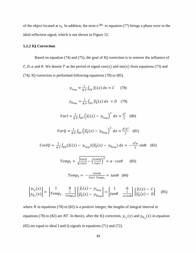
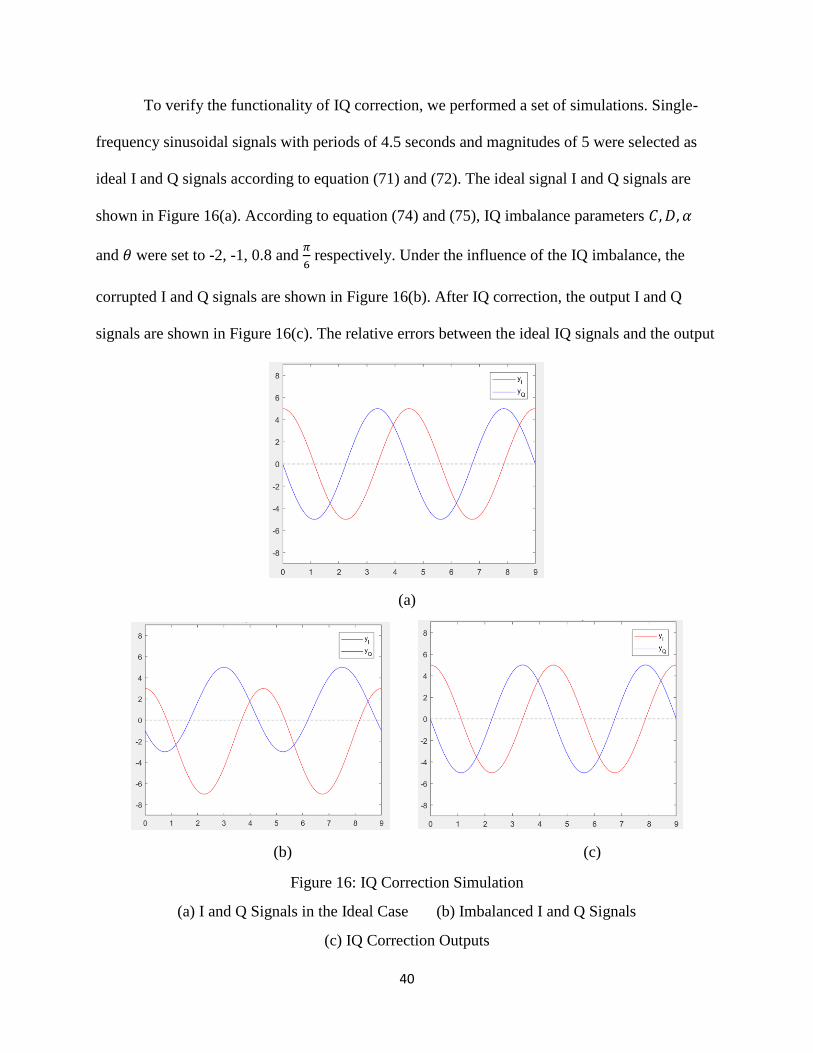
To verify the functionality of IQ correction, we performed a set of simulations. Single-
frequency sinusoidal signals with periods of 4.5 seconds and magnitudes of 5 were selected as
ideal I and Q signals according to equation (71) and (72). The ideal signal I and Q signals are
shown in Figure 16(a). According to equation (74) and (75), IQ imbalance parameters 𝐶, 𝐷, 𝛼
and 𝜃 were set to -2, -1, 0.8 and 𝜋
6 respectively. Under the influence of the IQ imbalance, the
corrupted I and Q signals are shown in Figure 16(b). After IQ correction, the output I and Q
signals are shown in Figure 16(c). The relative errors between the ideal IQ signals and the output
(a)
(b) (c)
Figure 16: IQ Correction Simulation
(a) I and Q Signals in the Ideal Case (b) Imbalanced I and Q Signals
(c) IQ Correction Outputs

41
signals from IQ correction were lower than 1.5%, which means the IQ correction was able to
provide an acceptable result.
5.3 Linear Range Error
In previous experiments, we observed reflector position errors in the range direction. As
seen in Figure 10, the absolute reflector positions from the experimental image were shifted to
the right in range from their expected positions in the simulated image. To have a further
understanding about reflector position error in range direction, we conducted the following
experiment:
(1) Fix the radar at a specific position on soccer field.
(2) Set a steel reflector at the same height as radar and move the reflector away from radar.
(3) Set down the distance between radar and reflector as 𝑟.
(4) Run the radar and collect data for 1000 pluses.
(5) Plot the range line by using experimental data from radar.
(6) Identify the peak corresponding to the reflector on the range line and record its distance
from the radar as 𝑟𝑒𝑥.
(7) Calculate the range error by ∆𝑟 = 𝑟𝑒𝑥 − 𝑟 and record the value of ∆𝑟.
(8) Move the reflector to a new position and repeat steps (3) to (7).
By moving around the reflector to different positions, we got different pairs of 𝑟 and ∆𝑟. Figure
17 shows the relationship between 𝑟 and ∆𝑟.
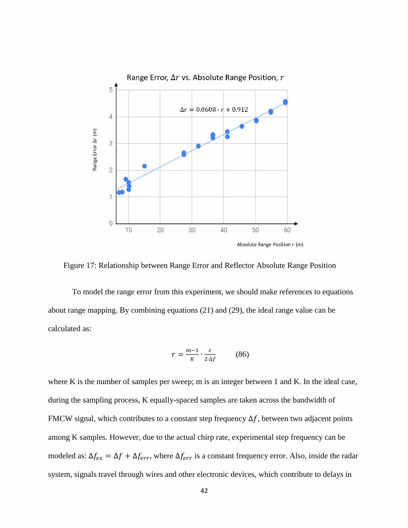
42
To model the range error from this experiment, we should make references to equations
about range mapping. By combining equations (21) and (29), the ideal range value can be
calculated as:
𝑟 =𝑚−1
𝐾∙𝑐
2∙∆𝑓 (86)
where K is the number of samples per sweep; m is an integer between 1 and K. In the ideal case,
during the sampling process, K equally-spaced samples are taken across the bandwidth of
FMCW signal, which contributes to a constant step frequency ∆𝑓, between two adjacent points
among K samples. However, due to the actual chirp rate, experimental step frequency can be
modeled as: ∆𝑓𝑒𝑥 = ∆𝑓 + ∆𝑓𝑒𝑟𝑟, where ∆𝑓𝑒𝑟𝑟 is a constant frequency error. Also, inside the radar
system, signals travel through wires and other electronic devices, which contribute to delays in
Figure 17: Relationship between Range Error and Reflector Absolute Range Position
43
signal communication. Delays in signal communication bring inaccuracies in range mapping and
therefore result in range errors. Since the hardware architecture of radar system is fixed, we can
model the hardware delays as a constant factor 𝑟0. Combining the discussions above, we can
model the experimental range value, 𝑟𝑒𝑥 as:
𝑟𝑒𝑥 =𝑚−1
𝐾∙
𝑐
2∙(∆𝑓+∆𝑓𝑒𝑟𝑟)+ 𝑟0 (87)
Mathematical expression of ∆𝑟 in Figure 15 can be gained by subtracting 𝑟 in equation (86) from
𝑟𝑒𝑥 in equation (87) and the slope in Figure 17 contains information about ∆𝑓𝑒𝑟𝑟 while the
intercept is related to 𝑟0.
The weakness of this range error experiment was that at each position, we only measured
𝑟 and 𝑟𝑒𝑥 for one time, rather than took multiple measurements and calculated the average. If the
linear relationship between range and range error were verified by more reliable experiments, the
range error would be removed by incorporating the linear relationship into the image processing
software, as correction to 𝑟0 and ∆𝑓.
5.4 Motion Error
In the SAR system, an accurate motion measurement is necessary to the constructions of
high-quality images. In this project, GPS unit is responsible for the motion measurement.
However, GPS unit in the SAR system is susceptible to errors. Errors in GPS data are called
“motion errors,” which bring attenuations to the qualities of SAR images. Figure 18 shows the
influence of motion error to the SAR system.
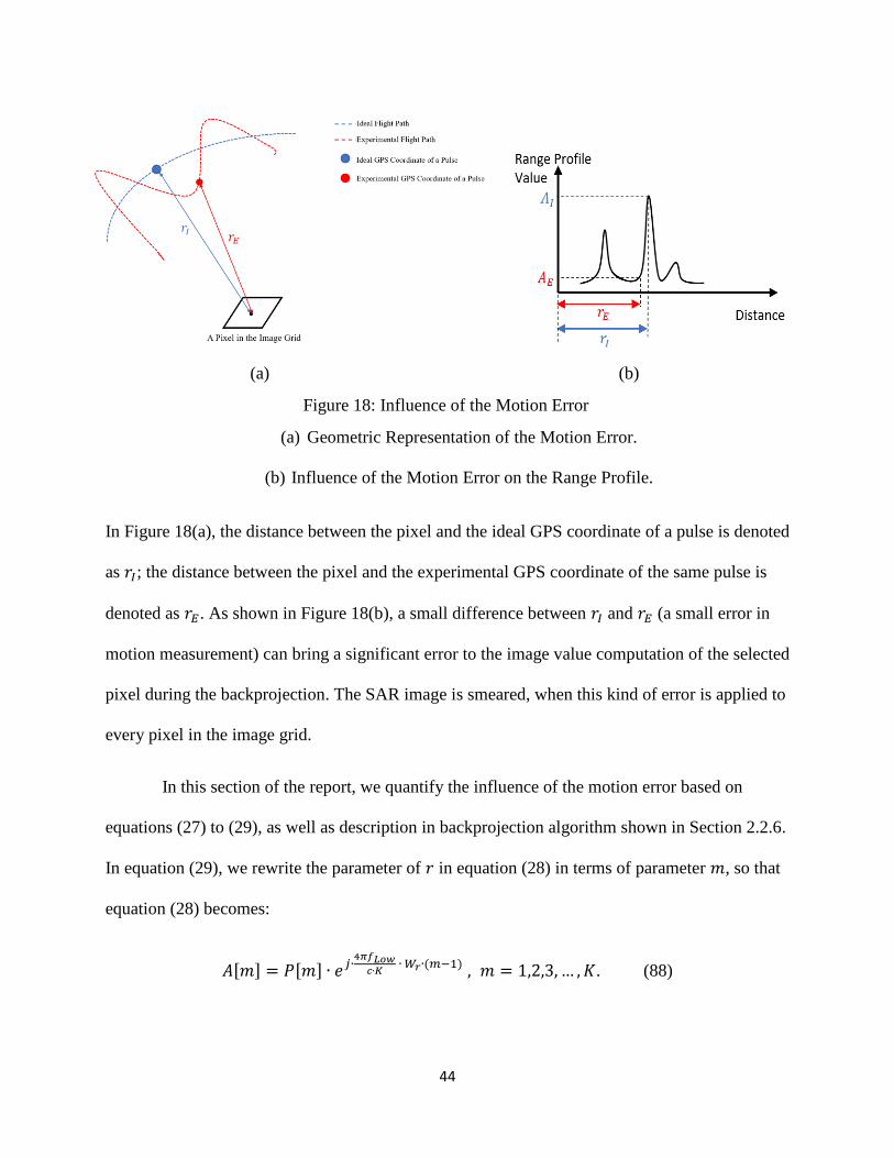
44
In Figure 18(a), the distance between the pixel and the ideal GPS coordinate of a pulse is denoted
as 𝑟𝐼; the distance between the pixel and the experimental GPS coordinate of the same pulse is
denoted as 𝑟𝐸. As shown in Figure 18(b), a small difference between 𝑟𝐼 and 𝑟𝐸 (a small error in
motion measurement) can bring a significant error to the image value computation of the selected
pixel during the backprojection. The SAR image is smeared, when this kind of error is applied to
every pixel in the image grid.
In this section of the report, we quantify the influence of the motion error based on
equations (27) to (29), as well as description in backprojection algorithm shown in Section 2.2.6.
In equation (29), we rewrite the parameter of 𝑟 in equation (28) in terms of parameter 𝑚, so that
equation (28) becomes:
𝐴[𝑚] = 𝑃[𝑚] ∙ 𝑒𝑗∙4𝜋𝑓𝐿𝑜𝑤𝑐∙𝐾
∙ 𝑊𝑟∙(𝑚−1) , 𝑚 = 1,2,3, … , 𝐾. (88)
(a) (b)
Figure 18: Influence of the Motion Error
(a) Geometric Representation of the Motion Error.
(b) Influence of the Motion Error on the Range Profile.
45
In ideal case for a single pixel shown in Figure 18(a), the distance between a selected pixel and
the SAR system is 𝑟𝐼. According to equation (29), the index, 𝑚𝐼, corresponding to 𝑟𝐼 is:
𝑚𝐼 =𝑟𝐼𝐾
𝑊𝑟+ 1. (89)
Therefore, the ideal image value of the selected pixel is:
𝐼𝑚 = 𝐴[𝑚𝐼] = 𝑃[𝑚𝐼] ∙ 𝑒𝑗∙4𝜋𝑓𝐿𝑜𝑤𝑐∙𝐾
∙ 𝑊𝑟∙(𝑚𝐼−1). (90)
In Figure 18(a), the experimental distance between a selected pixel and the SAR system is 𝑟𝐸.
The relationship between 𝑟𝐸 and 𝑟𝐼 can be expressed as:
𝑟𝐸 = 𝑟𝐼 + ∆𝑟. (91)
The index, 𝑚𝐸 corresponding to 𝑟𝐸 can be computed by equation (29):
𝑚𝐸 =𝑟𝐸𝐾
𝑊𝑟+ 1 (92)
𝑚𝐸 =𝑟𝐼𝐾
𝑊𝑟+ 1 +
∆𝑟∙𝐾
𝑊𝑟= 𝑚𝐼 +
∆𝑟∙𝐾
𝑊𝑟 . (93)
The experimental image value of the selected pixel is:
𝐼 = 𝐴[𝑚𝐸] = 𝑃[𝑚𝐸] ∙ 𝑒𝑗∙4𝜋𝑓𝐿𝑜𝑤𝑐∙𝐾
∙ 𝑊𝑟∙(𝑚𝐸−1). (94)
Rewrite 𝑚𝐼 in equation (90) in terms of 𝑚𝐸 according to equation (93), equation (90) becomes:
𝐼𝑚 = 𝑃[𝑚𝐸 − ∆𝑟∙𝐾
𝑊𝑟] ∙ 𝑒𝑗∙
4𝜋𝑓𝐿𝑜𝑤𝑐∙𝐾
∙ 𝑊𝑟∙(𝑚𝐸−1) ∙ 𝑒−𝑗4𝜋𝑓𝐿𝑜𝑤 ∆𝑟
𝑐 (95)
By combining equations (95) and (94), the result is:
46
𝐼𝑚
𝐼 =𝑃[𝑚𝐸 −
∆𝑟 ∙ 𝐾𝑊𝑟
] ∙ 𝑒−𝑗4𝜋𝑓𝐿𝑜𝑤 ∆𝑟
𝑐
𝑃[𝑚𝐸]
𝐼𝑚 = 𝐼 ∙ 𝑃[𝑚𝐸−
∆𝑟∙𝐾
𝑊𝑟]
𝑃[𝑚𝐸]∙ 𝑒−𝑗
4𝜋𝑓𝐿𝑜𝑤 ∆𝑟
𝑐⏟
𝐷(∆𝑟)𝑒𝑗𝜙(∆𝑟)
(96)
where 𝐷(∆𝑟) is the magnitude component of the error factor and 𝑒𝑗𝜙(∆𝑟) is the phase.
In theory, if the value of ∆𝑟 can be accurately determined, we were able to recover the ideal range
profile from the experimental range profile based on equation (96), such that the negative influences from
the motion errors on the SAR images can be removed. However, in reality, the accurate value of ∆𝑟 is
difficult to compute, which means recovering the ideal range profile directly from the experimental one is
not addressable.
Also, the autofocus algorithm mentioned in Chapter 3 above cannot solve the problems associated
with the motion errors. When errors are taken into account, the basic signal model of the autofocus
algorithm is shown in equation (34), which can be further expanded as:
𝑰𝒌 =
[
𝐼𝑚𝑘,1 ∙ 𝑒𝑗𝜙𝑘
𝐼𝑚𝑘,2 ∙ 𝑒𝑗𝜙𝑘
⋮𝐼𝑚𝑘,(𝑁𝑥×𝑁𝑦) ∙ 𝑒
𝑗𝜙𝑘]
, 𝑘 = 1,2,3, … ,𝑁𝑝 (97)
where 𝐼𝑚𝑘,𝑖 represents the ideal image value of the 𝑖𝑡ℎ pixel from the 𝑘𝑡ℎ pulse and 𝑒𝜙𝑘 is the
phase error associated with the 𝑘𝑡ℎ pulse. According to equation (97), there are two important
characteristics of the basic signal model:
(1) The error applied to each pixel of the image corresponding to a specific pulse is purely
phase error, with a constant magnitude of 1.
(2) All pixels of the image corresponding to a specific pulse have the same phase error.
47
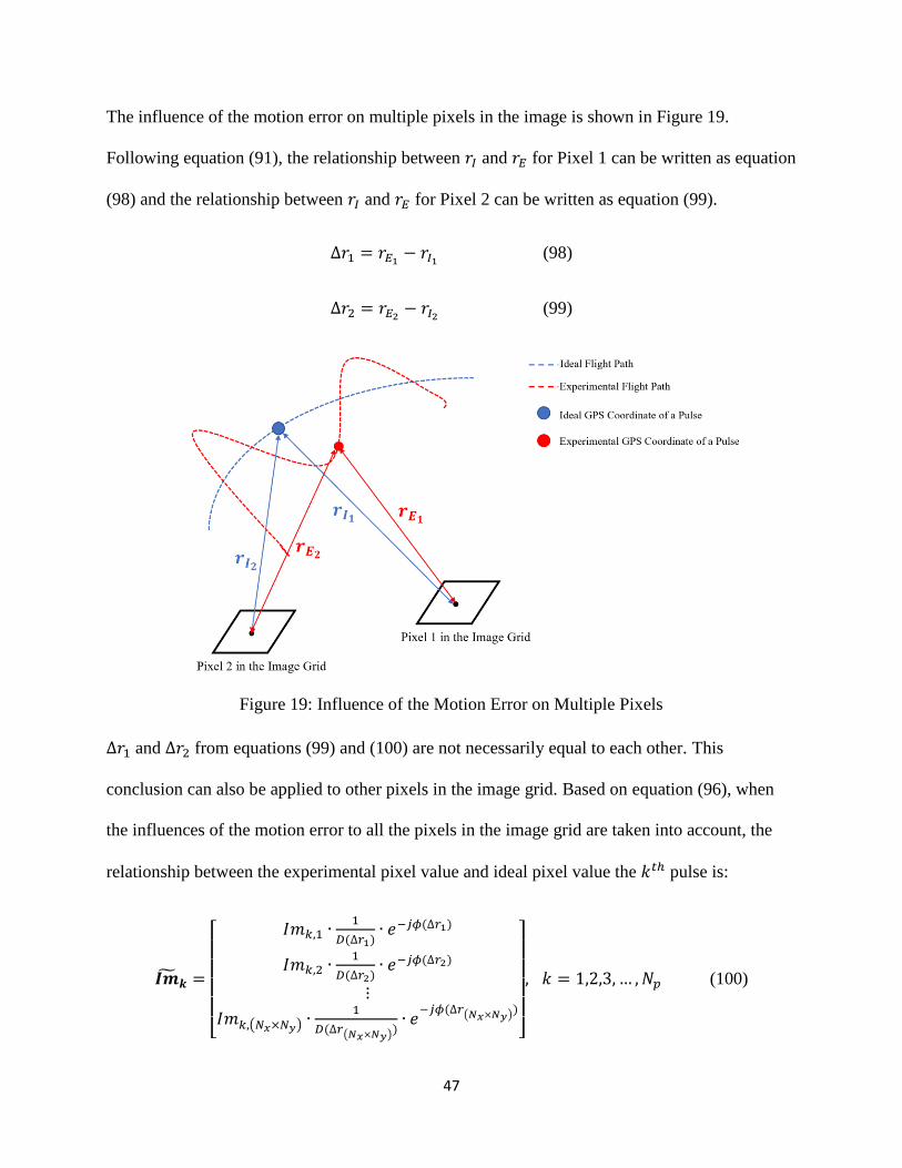
The influence of the motion error on multiple pixels in the image is shown in Figure 19.
Following equation (91), the relationship between 𝑟𝐼 and 𝑟𝐸 for Pixel 1 can be written as equation
(98) and the relationship between 𝑟𝐼 and 𝑟𝐸 for Pixel 2 can be written as equation (99).
∆𝑟1 = 𝑟𝐸1 − 𝑟𝐼1 (98)
∆𝑟2 = 𝑟𝐸2 − 𝑟𝐼2 (99)
∆𝑟1 and ∆𝑟2 from equations (99) and (100) are not necessarily equal to each other. This
conclusion can also be applied to other pixels in the image grid. Based on equation (96), when
the influences of the motion error to all the pixels in the image grid are taken into account, the
relationship between the experimental pixel value and ideal pixel value the 𝑘𝑡ℎ pulse is:
𝑰𝒌 =
[ 𝐼𝑚𝑘,1 ∙
1
𝐷(∆𝑟1)∙ 𝑒−𝑗𝜙(∆𝑟1)
𝐼𝑚𝑘,2 ∙1
𝐷(∆𝑟2)∙ 𝑒−𝑗𝜙(∆𝑟2)
⋮
𝐼𝑚𝑘,(𝑁𝑥×𝑁𝑦) ∙1
𝐷(∆𝑟(𝑁𝑥×𝑁𝑦))∙ 𝑒−𝑗𝜙(∆𝑟(𝑁𝑥×𝑁𝑦)
)
]
, 𝑘 = 1,2,3, … ,𝑁𝑝 (100)
Figure 19: Influence of the Motion Error on Multiple Pixels

48
where 𝐼𝑚𝑘,𝑖 represents the ideal image value of the 𝑖𝑡ℎ pixel from the 𝑘𝑡ℎ pulse; 1
𝐷(∆𝑟𝑖) is the
magnitude error associated with the 𝑖𝑡ℎ pixel from the 𝑘𝑡ℎ pulse; 𝑒−𝑗𝜙(∆𝑟𝑖) is the phase error
associated with the 𝑖𝑡ℎ pixel from the 𝑘𝑡ℎ pulse. Since ∆𝑟1, ∆𝑟2, …, ∆𝑟(𝑁𝑥×𝑁𝑦) in equation (100)
are not necessarily equal to each other, the error factors 1
𝐷(∆𝑟𝑖)∙ 𝑒−𝑗𝜙(∆𝑟𝑖) for different values of 𝑖
are not necessarily equal to each other.
The comparison between equations (97) and (100) shows that equation (100) does not
satisfy the two important characteristics from (97). In other words, the influences of the motion
error to the SAR image violate the basic assumption of the proposed autofocus algorithm in Chapter
3 and therefore, the autofocus algorithm cannot solve the problems associated with the motion errors.
49
CHAPTER 6: Conclusion and Future Work
In this project, we implemented backprojection and autofocus algorithms in image
processing software for a drone-SAR system. Based on radar and GPS data from a series of
experiments, we demonstrated that the software could construct SAR images with high
resolution. Although in general, experimental SAR images matched well with expectations, we
observed the effect of errors on the SAR images. Additional tests of the drone-SAR system not
only provided us with a further understanding of these errors, but also allowed us to correct some
errors by calibrating parameters in the imaging software.
Based on the success from the team, there are two directions for future works. The first
direction for future work is to improve the performance of 2-D image construction for the current
drone-SAR system. Enhancements include: Kalman filtering [14] for fusion of GPS and
accelerometer data for improved position accuracy; wi-fi control of data acquisition; improved
calibration of chirp rate and signal delay; etc. The second direction for future work is to find new
applications for the current drone-SAR system. Due to the capacity from SAR system to provide
vision under situations when optical systems are not available, as well as the high-degree of
flexibility brought by the drone platform, the drone-SAR system can be extensively applied to
different fields, such as constructing 3-D SAR images, security monitoring, industry supervision,
emergency response, navigation without GPS, interferometric SAR [15], etc.

50
CHAPTER 7: Reference
[1] A. W. Doerry and F. M. Dickey, "Synthetic aperture radar," Optics and Photonics News,
vol. 15, no. 11, pp 28-33, 2014.
[2] D. Chen, T. Dean, B. Fair and L. Newton, “Light-weight SAR imaging system for
UAS: ECE 4901 final report.” SAR Quadcopter Project, 2017. [Online]. Available:
https://drive.google.com/drive/folders/0BzYlqaSHVRKNS3FUS2dHcHc1VDA.
[Accessed: Feb. 10, 2018].
[3] B. Downs, A. Pycraft, and L. Smith, “Synthetic aperture radar on an unmanned aircraft
system: ECE 4901 final report.” SAR Quadcopter Project, 2018. [Online]. Available:
https://drive.google.com/drive/folders/1cN1RCiVxxn8ZJKRT9c_fLdZ4ks87_DV6.
[Accessed: Oct. 4, 2018].
[4] Federal Aviation Administration, “FAA regulations,” faa.gov, Oct. 27, 2017. [Online].
Available: https://www.faa.gov/regulations_policies/faa_regulations/. [Accessed: Aug.
19, 2018].
[5] Federal Communications Commission. “Rules & regulations for title 47,” fcc.gov, Aug.
16, 2018. [Online]. Available: https://www.fcc.gov/wireless/bureau-divisions/
technologies-systems-and-innovation-division/rules-regulations-title-47. [Accessed: Aug.
19, 2018].
[6] The Ohio State University. “Use of unmanned aircraft systems (UAS),” oaa.osu.edu, Apr.
2, 2018. [Online]. Available: https://oaa.osu.edu/sites/default/files/uploads/
policies/UAS-Policy.pdf. [Accessed: Aug. 19, 2018].
51
[7] L.A. Gorham and L.J. Moore, “SAR image formation toolbox for MATLAB,” in Proc. of
SPIE Defense Security, and Sensing, 5-9 Apr. 2010, Orlando, Florida, United States
[Online]. Available: https://www.spiedigitallibrary.org/conference-proceedings-of-
spie/7699/769906/SAR-image-formation-toolbox-for-MATLAB/10.1117/12.855375.full.
[Accessed: Aug. 19, 2018].
[8] J. N. Ash, "An autofocus method for backprojection imagery in synthetic aperture radar,"
IEEE Geoscience and Remote Sensing Letters, vol. 9, no. 1, pp. 104-108, Jan. 2012.
[9] D.C. Munson, J.D O'Brien, and W.K Jenkins, "A tomographic formulation of spotlight-
mode synthetic aperture radar," Proceedings of the IEEE, vol. 71, no. 8, pp. 917-925,
Aug. 1983.
[10] The Mathworks Inc., “Inverse fast Fourier transform,” MATLAB Documentation,
R2018a, 2018. [Online]. Available: https://www.mathworks.com/help/matlab/ref/
ifft.html. [Accessed: Aug.19, 2018].
[11] J.C. Hart, “Distance to an ellipsoid,” in Graphics Gem IV, San Mateo, CA: Morgan
Kaufmann, 1994.
[12] The Mathworks Inc., “Window function gateway,” MATLAB Documentation, R2018b,
2018. [Online]. Available: https://www.mathworks.com/help/signal/ref/window.html.
[Accessed: Oct.19, 2018].
[13] The Mathworks Inc., “Blackman window,” MATLAB Documentation, R2018b, 2018.
[Online]. Available: https://www.mathworks.com/help/signal/ref/blackman.html.
[Accessed: Oct.19, 2018].

52
[14] R.G. Brown and P.Y. Hwang, Introduction to Random Signals and Applied Kalman
Filtering, Vol.3. NY: Wiley, 1992.
[15] M.A. Richards, “A beginner’s guide to interferometric SAR concepts and signal
processing [AESS Tutorial IV],” IEEE Aerospace and Electronic System Magazine, vol.
22, no. 9, pp. 5-29, Oct. 2007
[16] W.G. Carrara, R.S. Goodman and R.M. Majewski, Spotlight Synthetic Aperture Radar
Signal Processing Algorithms, Norwood, MA: Artech House, 1995.