1

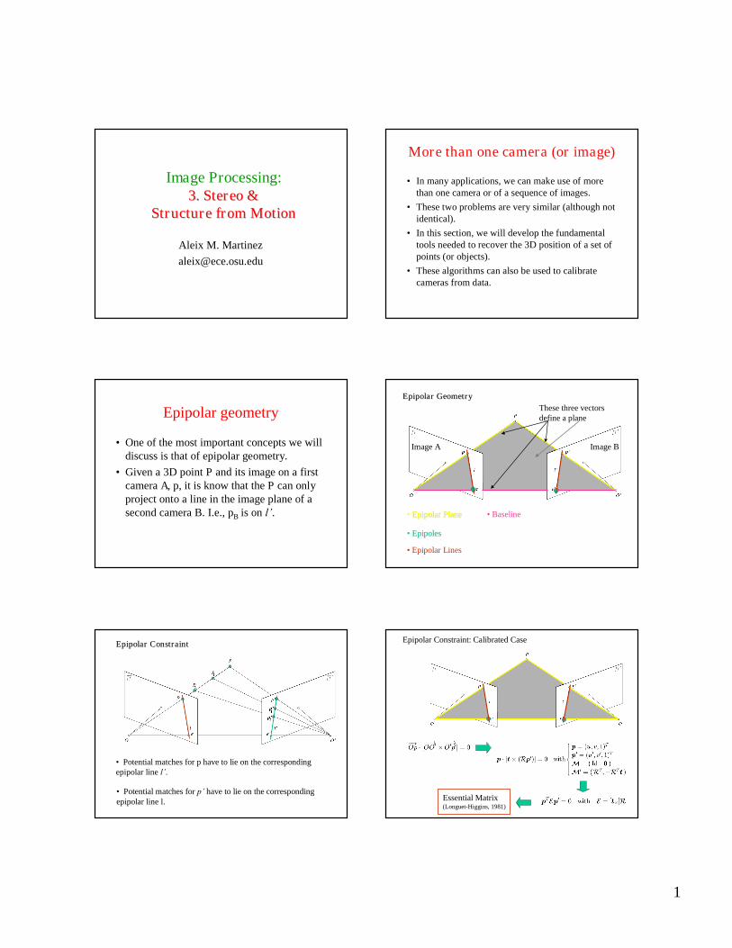
Image Processing:3.3. Stereo &Stereo &

Structure from MotionStructure from Motion

Aleix M. Martinezaleix@ece.osu.edu

More than one camera (or image)

•In many applications, we can make use of morethan one camera or of a sequence of images.•These two problems are very similar (although not

identical).•In this section, we will develop the fundamental

tools needed to recover the 3D position of a set ofpoints (or objects).•These algorithms can also be used to calibrate

cameras from data.

Epipolar geometry

•One of the most important concepts we willdiscuss is that of epipolar geometry.•Given a 3D point P and its image on a first

camera A, p, it is know that the P can onlyproject onto a line in the image plane of asecond camera B. I.e., pB is onl’.

EpipolarEpipolar GeometryGeometry

•EpipolarEpipolar PlanePlane

•EpipolesEpipoles

•Epipolar Lines

•Baseline

These three vectorsdefine a plane

Image A Image B

EpipolarEpipolar ConstraintConstraint

•Potential matches for p have to lie on the correspondingepipolar linel’.

•Potential matches forp’have to lie on the correspondingepipolar line l.

Epipolar Constraint: Calibrated Case

Essential Matrix(Longuet-Higgins, 1981)

2

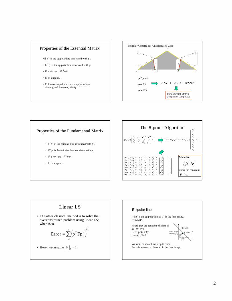
Properties of the Essential Matrix

•Ep’ is the epipolarline associated with p’.

•E p is the epipolar line associated with p.

•Ee’=0 and E e=0.

•E is singular.

•E has two equal non-zero singular values(Huang and Faugeras, 1989).

T

T

EpipolarEpipolar Constraint: Uncalibrated CaseConstraint: Uncalibrated Case

Fundamental Matrix(Faugeras and Luong, 1992)

Properties of the Fundamental Matrix

•Fp’ is the epipolarline associated with p’.

•F p is the epipolar line associated with p.

•Fe’=0 and F e=0.

•F is singular.

T

T

|F | =1.

Minimize:

under the constraint2

The 8-point Algorithm

Linear LS

•The other classical method is to solve theoverconstrained problem using linear LS;when n>8.

•Here, we assume

2

1

'

n

ii

T FError i pp

.1F

F

Epipolar line:

),(),(

baba

n

directionnormalUnit

Tcbal ),,(

),( bac

:linetheto

originofDistance Tvup )1,,(

l=Fp’ is the epipolar line of p’ in the first image.l=(a,b,c)T.

Recall that the equation of a line isau+bv+c=0.Here, p=(u,v,1)T.Hence, pTl=0

We want to know how far p is from l.For this we need to draw a l in the first image.

3

% Assume p, p_prime are two corresponding image points.% p=(u,v,1); p_prime=(u_prime,v_prime,1);

epipolar_line = F * p_prime;a = epipolar_line(1);b = epipolar_line(2);c = epipolar_line(3);

% Consider a region around p in two cases due to different slope% ‘length’ is half the line segment length you want to draw

if(abs(a)<abs(b))d = length/sqrt((a/b)^2+1);drawpoint = [u-d u+d ; ((-c - a*(u-d))/b (-c - a*(u+d))/b ];

elsed = length/sqrt((b/a)^2+1);drawpoint = [(-c - b*(v-d))/a (-c - b*(v+d))/a ; v-d v +d ];

endplot(drawpoint(1,:), drawpoint(2,:));

Epipolar line:

p

u+du-d

(-c - a*(u-d) ) /b

(-c - a*(u+d) ) /b

To draw the line, it is convenient to choose an interval.

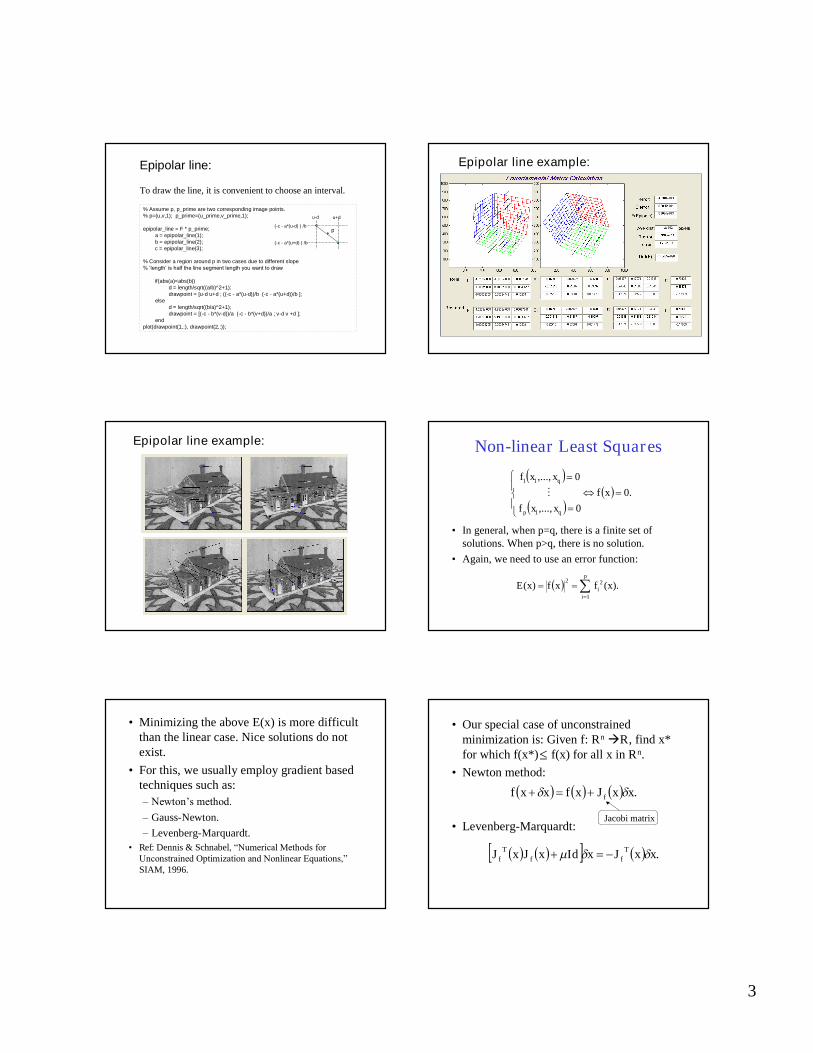
Epipolar line example:

Epipolar line example: Non-linear Least Squares

•In general, when p=q, there is a finite set ofsolutions. When p>q, there is no solution.•Again, we need to use an error function:

.

0,...,

0,...,

1

11

0xf

qp

q

xxf

xxf

p

iifE

1

22).()( xxfx

•Minimizing the above E(x) is more difficultthan the linear case. Nice solutions do notexist.•For this, we usually employ gradient based

techniques such as:–Newton’s method.–Gauss-Newton.–Levenberg-Marquardt.

•Ref: Dennis & Schnabel, “Numerical Methods for Unconstrained Optimization and Nonlinear Equations,” SIAM, 1996.

•Our special case of unconstrainedminimization is: Given f: RnR, find x*for which f(x*) f(x) for all x in Rn.•Newton method:

•Levenberg-Marquardt:

.xxxfxxf f J

.xxxIdxx fff TT JJJ

Jacobi matrix

4

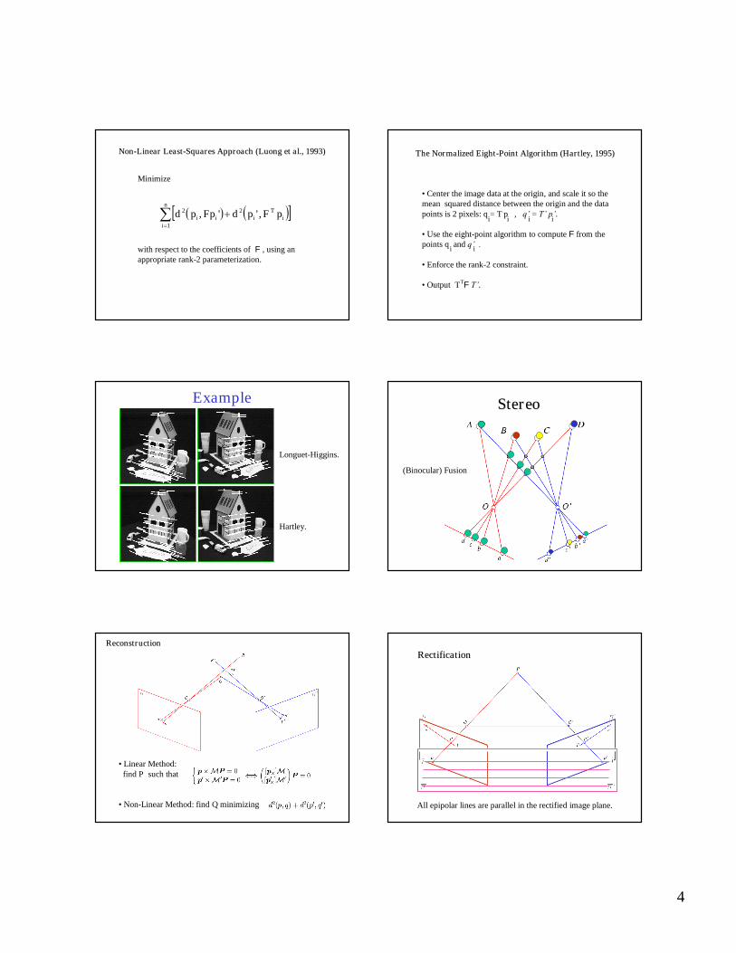
NonNon--Linear LeastLinear Least--Squares Approach (Squares Approach (LuongLuong et al., 1993)et al., 1993)

Minimize

with respect to the coefficients of F , using anappropriate rank-2 parameterization.

n

ii

Tiii pFpdFppd

1

22 ,'',

The Normalized EightThe Normalized Eight--Point Algorithm (Hartley, 1995)Point Algorithm (Hartley, 1995)

•Center the image data at the origin, and scale it so themean squared distance between the origin and the datapoints is 2 pixels: q = T p , q’=T’ p’.

•Use the eight-point algorithm to compute F from thepoints q andq’ .

•Enforce the rank-2 constraint.

•Output T FT’.T

i i i i

i i

Example

Longuet-Higgins.

Hartley.

StereoStereo

(Binocular) Fusion

ReconstructionReconstruction

•Linear Method:find P such that

•Non-Linear Method: find Q minimizing

RectificationRectification

All epipolar lines are parallel in the rectified image plane.

5

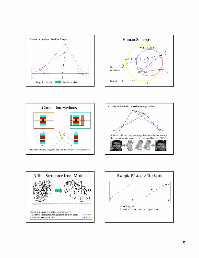
Reconstruction from Rectified ImagesReconstruction from Rectified Images

Disparity:d=u’-u. Depth: z = -B/d.

Human Stereopsis

Disparity: d = r-l = D-F.

d=0

d<0

Correlation Methods

Slide the window along the epipolar line untilw.w’is maximized.

Correlation Methods: Foreshortening ProblemsCorrelation Methods: Foreshortening Problems

Solution: add a second pass using disparity estimates to warpthe correlation windows, e.g. Devernay and Faugeras (1994).

AffineAffine Structure from MotionStructure from Motion

Reprinted with permission from “Affine Structure from Motion,” by J.J. (Koenderink and A.J.Van Doorn, Journal of the Optical Society of America A,8:377-385 (1990). 1990 Optical Society of America.

Given m pictures of n points, can we recover•the three-dimensional configuration of these points?•the camera configurations?

(structure)(motion)

Example: R as an Affine Space2

6

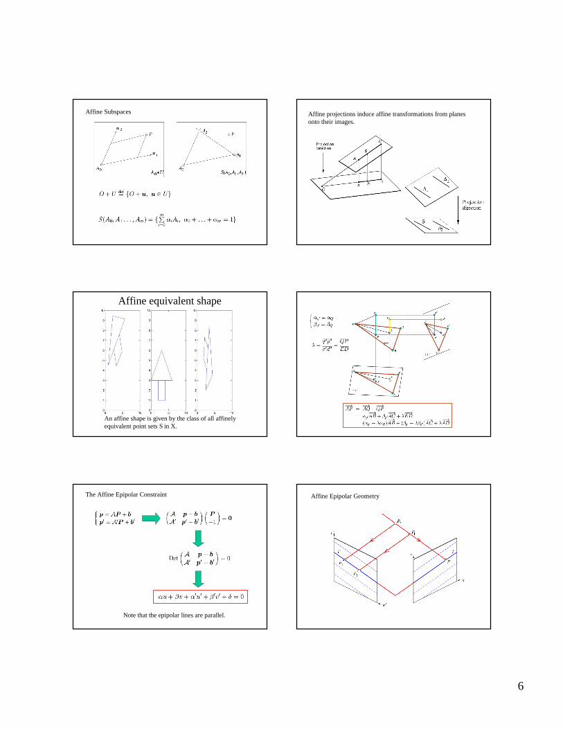
Affine Subspaces Affine projections induce affine transformations from planesonto their images.

Affine equivalent shape

An affine shape is given by the class of all affinelyequivalent point sets S in X.

The Affine Epipolar Constraint

Note that the epipolar lines are parallel.

Affine Epipolar Geometry

7

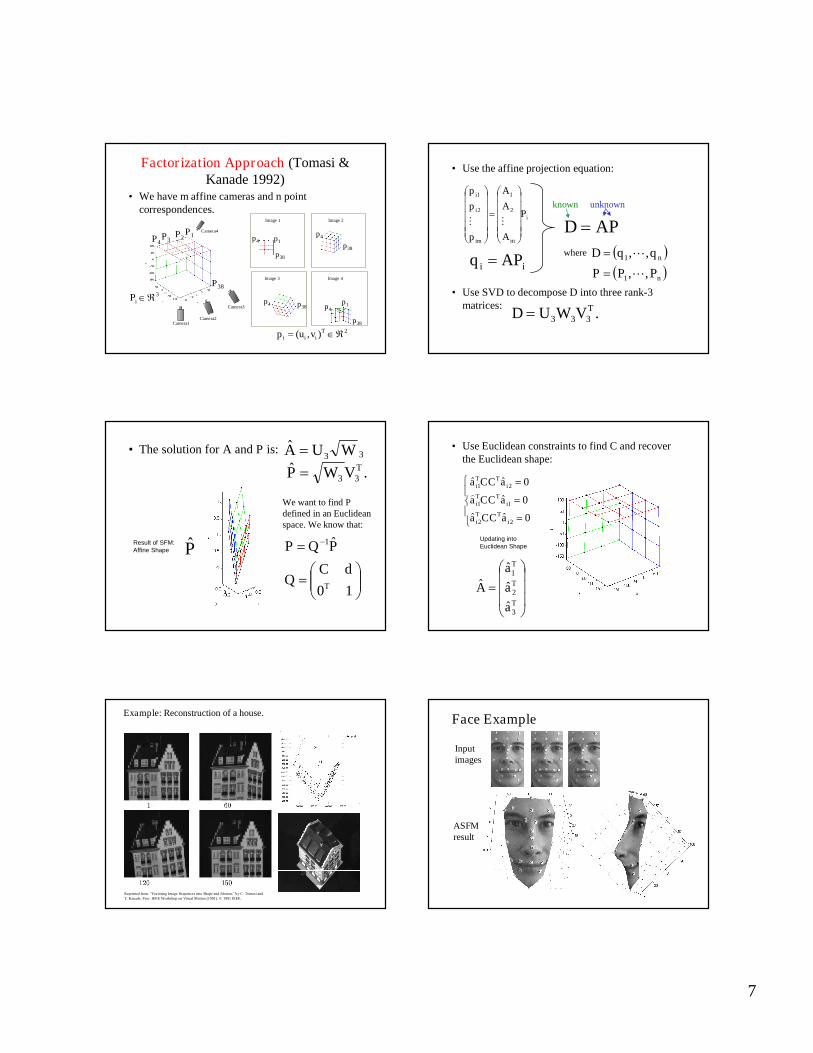
Factorization Approach (Tomasi &Kanade 1992)

•We have m affine cameras and n pointcorrespondences.

Camera1Camera2

Camera3

Camera4P1P3P2P4

P383P i

Image 1 Image 2

Image 3 Image 4

p1

p38

p4p38

p4

p38p4 p1

p38

p4

2),( Tiii vup

•Use the affine projection equation:

i

mim

i

i

P

A

A

A

p

p

p

2

1

2

1

ii APq

APD known unknown

where nqqD ,,1

nPPP ,,1 •Use SVD to decompose D into three rank-3

matrices: .333TVWUD

•The solution for A and P is: 33ˆ WUA

.ˆ33TVWP

Result of SFM:Affine Shape P̂

1

ˆ1

T0dC

Q

PQP

We want to find Pdefined in an Euclideanspace. We know that:

•Use Euclidean constraints to find C and recoverthe Euclidean shape:

0ˆˆ

0ˆ

0ˆˆ

22

11

21

iTT

i

iTT

i

iTT

i

aCCa

aCCa

aCCa

Updating intoEuclidean Shape

T

T

T

3

2

1

ˆˆˆ

ˆ

aaa

A

Example: Reconstruction of a house.

Reprinted from “Factoring Image Sequences into Shape and Motion,” by C. Tomasi andT. Kanade, Proc. IEEE Workshop on Visual Motion (1991). 1991 IEEE.

Face Example

Inputimages

ASFMresult

8

Figures by kind permission of Eric Grimson; further information can beobtained from his web site http://www.ai.mit.edu/people/welg/welg.html. Figures by kind permission of Eric Grimson; further information can be

obtained from his web site http://www.ai.mit.edu/people/welg/welg.html.

Figures by kind permission of Eric Grimson; further information can beobtained from his web site http://www.ai.mit.edu/people/welg/welg.html.

RenderingRenderingVolumetric Models -- Visual Hulls (Laurentini, 1995)

Reprinted from “Automatic Model Construction, Pose Estimation, and Object Recognition from Photographs Using Triangular Splines,”By S. Sullivan and J. Ponce, IEEE Trans. on Pattern Analysis and Machine Intelligence, 20(10):1091-1096 (1998). 1998 IEEE.

Reprinted from “Automatic Model Construction, Pose Estimation, and Object Recognition from Photographs Using Triangular Splines,”By S. Sullivan and J. Ponce, IEEE Trans. on Pattern Analysis and Machine Intelligence, 20(10):1091-1096 (1998). 1998 IEEE.

Augmented Reality Experiments

Reprinted from :Calibration-Free Augmented Reality,” by K. Kutulakos and J. Vallino, IEEETrans. On Visualization and Computer Graphics, 4(1):1-20 (1998). 1998 IEEE.

Courtesy of Kyros Kutulakos.

9

How about human perception?Can you recognize these faces?

Internal features

Sinha & Poggio 1996, 2002.

Final Note

•As a final note, it is important to know thatall the concepts seen so far can also bedescribed in nicer mathematical framework.•This is more complicated, but allows for

more powerful algorithms.•All algorithms seen so far can be described

within this framework.

Projective, Affine, andEuclidean spaces

•Projective transformations are the mostgeneral, and we are all familiar with them;i.e., a 2D picture of the 3D world.•Affine are more specific, where the line (or

plane) at infinity is specified.•A Euclidean transformation is one where

shapes are not distorted. This requires wedefine the absolute conic.

Projective Geometry•Recall, that a point (x,y)T can can expressed

in homogeneous coordinates as (x,y,1)T.•Here, (x,y,1)T and (2x,2y,2)T represent the

same point. In general, (kx,ky,k)T.•Points are defined up to scale: equivalent

class.•The points (x,y,0)T are said to be at infinity.•Homogeneous coordinates extend the

Euclidean space Rn to the projective spacePn.

•Points at infinity are not different to others.•Projective transformations are represented

as mappings of homogeneous coordinates:

where H is any non-singular matrix.•Points at infinity may not be preserved.•Since points at infinity are only an accident

of our notation, we can say that all pointsare created equal.•Properties such as parallelism do not apply.

HXX '

10

Affine Geometry•Start with P2 and draw a line. Define this as

the line at infinity.•Any two lines that cross at this line at

infinity are said to be parallel. E.g., thehorizon (in a image) is the line at infinity.•This is an affine space.•Any projective transformation that maps the

distinguished line in one space to thedistinguished line of another is an affinetransformation.

Euclidean Geometry•Shapes may not be preserved by affine

transformations.•The concept of a circle does not exist in

affine geometry. Ellipse are mapped toother ellipses.•Two ellipses (generally) cross at 4 points.•Circles are defined in Euclidean geometry.•Circles only cross at two points.•How can this be?

2D Euclidean: Circular points•The equation of a circle in homogeneous

coordinates (x,y,w)T is (x-aw)2+(y-bw)2=r2w2.Here the circle is centered at (a,b,1)T.•Note that (x,y,z)=(1, ,0) are solutions to this

equation. Complex solutions.•Furthermore, these solutions lie on the line at

infinity.•These two points are known as the circular

points. They define circles.•The circular points define Euclidean geom.

i

3D Euclidean Geometry•In 3D, we have spheres, rather than circles.•The intersection of two spheres is a circle.•This circle is at the plane at infinity, and

define 3D Euclidean geometry.•Because, this circle is a second degree curve,

x2+y2+z2=0 (with final homegeneouscoordinate 0), this is known as the absoluteconic.•This provides many additional properties,

such as perpendicularity of lines.

Further Reading

•Hartley & Zisserman, “Multiple View Geometry in ComputerVision,” Cambridge University Press; 2 edition,2004.•Faugeras, “Three-dimensionalComputer Vision,” MIT Press, 1993.