Image Inpainting: A Review of Early Work and

Introduction Of A Multilevel Approach

Kenneth Webster

January 14, 2015

1 Abstract

There are instances where an image has data missing from it, so some form of approximationneeds to be used to complete the image.In the literature, the approximating of missingdata is referred to as image inpainting. A solution to this problem is to use a localprocess that when applied to the image, gives an approximation to the missing data.In this paper, a multilevel approach is used in conjunction with a single-level solutionto the problem. This method has various advantages over other existing approachesdue to the fact it utilizes multiple levels. This allows for a more global understandingof the problem since the fine and coarse level information are both considered. Thismultilevel approach has the same order of computational complexity as the single-levelbase method being used. Here, the coarse solution is used as an initial approximationto the solution of the finer level. The order of the complexity is not increased, rather,the size of the coarser levels decreases in such a way that the summation of those sizesonly doubles the computational cost of the single-level problem.

2 Introduction

There is currently an explosive growth in the field of image processing. A new breakthrough is discovered in area of digital computation and telecommunication almostevery month. Noticeable developments came from the public as computers becameaffordable and new technologies such as smart phones and tablets now allowing theinternet to be accessed anywhere. As a result of this there has been a wave of instantinformation available to many homes and businesses. This information can usually befound in four forms: text, graphics, pictures, and multimedia presentations. Digitalimages are pictures whose visual information has been transformed into a computerready format that is made up of binary 1s and 0s. When referring to an image, it isunderstood that the image is a still picture that does not change over time unlike avideo. Digital images are being used for storing, displaying, processing and transmitting

1

information at an ever increasing frequency. So it is important that there be effectivelyengineered methods to allow for the efficient transmission, maintenance and improvementof the visual integrity of this digital information.

Image processing is an important topic of research due to its large amount of variedresearch and industrial applications. Many branches of science have sub disciplinesusing recording devices and sensors to capture image data from the world. The datais usually multidimensional and may be arranged in such a way to be viewable to us.Viewable datasets such as these may also be regarded as images and processed usingmethods that are currently in use in image processing, even if the datasets have notbeen obtained from visible light sources such as x-rays or MRI.

There are instances where an image has data missing from it. In the literature, theapproximating of missing data is referred to as image inpainting. A way to correctthe incomplete image is to use a local process that when applied to the image, givesan approximation to the missing data. In this paper, a multilevel approach is used inconjunction with another single-level solution to the problem. This method has variousadvantages over some other existing approaches because the multiple levels allow for amore global understanding of the problem since the fine and coarse level informationare both being considered. In addition, this multilevel approach has the same order ofcomputational complexity as the single-level method being used as a base. Here thecoarse solution is used as an initial approximation to the solution of the finer level. Theorder of the computational complexity is not increased since the size of the coarser levelsdecrease, in such a way that the summation of those sizes only doubles the computationalcost of the single-level problem. The approach allows for repeated iterations to get abetter approximation.

The noise in the image affects a critical step in the original single level algorithm. Theproblem often affected the final result to such an extent to be noticeably ‘wrong’ to thehuman eye. A solution to the problem could be achieved in the following ways:

• Use an image restoration technique focusing on edge preservation

• Techniques that damp/remove noise

Neither approach can satisfactorily solve the issue. The edge preservation techniquesare time costly, and ineffectively integrated into the framework. The damping/removingnoise algorithms, while time-cost effective, suffers from requiring user defined values andloss of edge information on the local scale. This paper explores an approach whichbetter solves the problem in a way that is less computationally intensive, and preservesthe edges on the local scale. The solution is line-space or 2θ space.

2

Figure 1: From left to right there is an object in the foreground of the image which isremoved then filled in such a way as to appear natural. Image courtesy of [18]

3 Research Problem

Advances in technology allow a scene to be captured in the form of a picture stored in adigital format. This format allows images to be altered with the aid of a computer. Oftenwhen a picture is taken a part of the scene is judged to be undesirable and removed.The problem is how should this now missing information be completed without causingany other undesirable parts to appear within the scene? Figure 1 is the image of a birdat the edge of a road. The bird is deemed to be undesirable in the image so the usermust manually remove the bird, creating a hole. This hole is called the mask in theliterature. The mask is completed by using an approximation. Once the approximationis made, the image is said to be complete. One difficulty in completing an image ismatching multiple textures. In image processing, a texture gives us information aboutthe spatial arrangement of colour or intensities in parts of an image. In Figure 1 thereare two distinct textures that border on the hole that was the bird. There is grass andthere is road. Grass has many vertical lines that are relatively thin compared to theresolution of the image. This image contains low amplitude but high frequency changesin a local area. The road is smooth in a local area but has shadows cast on it thatchange the intensity over a global area. A good approximation for the missing datawould match both of these textures in the mask. Mathematically this problem is saidto be ill-defined because there does not exist a unique solution to the problem sincebeing a ‘correct’ solution comes down to an individual preference for how the missingdata is approximated. The preference for an image completion is to have the humanbrain perceive no artificially induced discrepancies, commonly referred to as wanting animage to ‘look natural’. It is difficult to solve since the words ‘look natural’ are not welldefined mathematically, so forming an equation to solve can be time consuming and itis quite difficult to know exactly what information our brain is using to determine if the

3

image ‘looks natural’ or not. In the literature so far, it has proved important that thetextures be replicated and continuing structures that extend into the missing data shouldbe completed as well. Those two aspects should be maintained on a local and globalscale simultaneously for the image to ‘look natural’. The main idea of the method beingpresented in this paper is to achieve very simple structure completion by propagatingtextures into the unknown region while maintaining a balance with respect to the globaland local scale. Employing a given image completion method that works on a local scalewithin a suitable multilevel framework should achieve a completion that works globallyand it should therefore improve the robustness of the local method substantially. Themethod will be used to complete synthetic and natural images.

4 Previous Work

Inpainting methods can generally be sorted into several categories. One approach is toview the image as the domain of a problem where the values in the grid are the discretizedversion of a PDE solution that is sought [3, 4, 11]. This approach utilizes numericalmethods to solve diffusion equations by extending the image into the missing data regioniteratively. In [7], convolution was used to propagate the diffusion to achieve a fasterrestoration compared to previous PDE methods. In [24] the algorithm approximatedthe missing data one pixel at a time by using the mean and variance of a block ina multi-resolution framework. It was proposed in [23] to use edge detection methodsto approximate the structure of the data in the missing region. Once the structure iscompleted, only then is the rest of the missing data approximated. All of these methodsproduce very smooth results inside the missing data region which rarely matches thesmoothness of the known parts of the image. These methods work well when the regionof missing data is small in size compared to the entire domain. A second approachto the problem is to use texture synthesis to fill regions of missing data that are largecompared to the domain, with texture sampled from the known data in the image. Thisapproach was used by [9, 15, 19, 27] to approximate the missing data pixel by pixel.The value of the pixel was determined by sampling its local neighbourhood and usinga best case match found in the known data of the image. One way to speed up thisprocess involves copying a small region of known data to the missing data. The authorsof [2, 15] define these regions as patches or blocks and the process of approximating themissing data as filling. From this, it is unclear in what order the mask should be filled.The order should create an image that minimizes seams between the patches. Whatconstitutes a seam cannot be properly defined since it is a judgment of the human eye,but in practice the idea is to minimize any ‘noticeable’ pattern of discontinuities in theimage that matches the pattern of the filling. [22] determines the shapes and whichorder to fill them in by using a graph cutting algorithm. The problem of determiningthe order to fill the missing data was shown to be relevant by Harrison in [19], where thepriority of the next patch in the missing region to be filled was chosen by the entropyof its local neighbourhood. A combination of PDE and texture patching is used in [6].

4

Images were defined to be a combination of structure and texture, and completion ofthe mask is done on each component separately. Once the image is decomposed into twoparts, a PDE method from [4] is used to fill the structured image and a texture synthesismethod from [14] is used for the textures of the decomposed image. Once both partsare completed they are recombined to form the completion of the original image. Thismethod captures both structure and textural data when filling in the image. However,since it uses a PDE diffusion model, it must be restricted to filling in small regions ofmissing data otherwise it suffers the same problem as the previous algorithms. In [10]the missing region was filled using a pyramid search in the known data, but the patchsize was arbitrary, so there may have been better choices available. [25] included a formof guidance from the user where the user would extend the important structures intothe missing region. The algorithm would then fill in the gaps using Belief Propagation[17] around the structures, and the remaining parts of the missing region would be filledusing texture synthesis patch by patch. However, the major issue of this algorithm isthat it requires supervision by the user, which may be time-consuming and inefficient.

The method presented in this paper is meant to compete with the method of Gazit [20].Gazit uses multiple levels where each level has undergone edge-preserving smoothing ofthe previous level. Gazit uses the approach of Criminisi [12] to determine the order inwhich to fill the mask. A matching patch is selected by considering the Mean SquareError (MSE) on all levels. The matching patch provides and initial guess that is refinedby moving from the smoothest level to the original image. Then a new patch in themask to fill is chosen according to the Criminisi [12] algorithm and the whole processis repeated until the mask is completely filled in. One of the purposes of the algorithmpresented in this paper is to lower the computational complexity necessary to match thesingle level algorithm of Criminisi [12] by using a multigrid framework, where the gridson the different levels are decreasing in size by a factor of two in each dimension. TheGazit [20] levels are all the same size. Using levels of the same size avoids problemsencountered using decreasing grid sizes. They are described later in this paper.

The algorithm of this paper uses the method of [12] which is a computationally feasiblemethod with complexity O(mnlog(n)) where m is the number of patches and n is thenumber of pixels defined by the resolution of the image. The algorithm uses exemplar-basedsynthesis to patch the missing region and the order of the patching is calculated by thedirection and size of gradients that border the boundary of the missing region. The goalof Criminisi is to extend the linear structures located along the boundary of the missingregion into the missing region with texture synthesis so that both structure and textureare filled in at the same time.

The method presented in this paper uses the single-level patching [12] as the smoother ofa multigrid cycle for solving elliptic PDEs. Using the PDE solver framework ensures thatthe order of computational complexity is not increased from the single-level patching of[12], while improving the final results.

5

5 Notation

Let I denote a digital image represented by a matrix of real numbers on a set of pixels Ω.Let Ω be partitioned into two regions Ω = Ωk∪Ωm where Ωk is the subset of pixels whereI is known and Ωm is the subset of pixels where I is unknown. This unknown region isthe missing data and in the literature is referred to as the mask, see figure below. Analgorithm which fills in the missing data is referred to as a completion algorithm. Itcan be defined as a function C such that J = C(I(Ω)) satisfies J(Ωk) = I(Ωk), whereC applied on an image with missing data returns an identical image except inside themissing region which now has been approximated. C approximates the missing data inthe image I with the goal of the now-filled missing region not appearing ‘unnatural’ tothe human eye, which is a subjective goal.

6 Bertalmio PDE method, [5]

6.1 Contribution

The algorithms devised for film restorations are not appropriate because they rely onthe mask which is small in comparison with the image and they rely on the existenceof information from several frames. Algorithms based on texture synthesis can fill largeregions, but require the user to specify what texture to put where the technique theauthors propose does not require any user intervention, once the region to be inpaintedhas been selected the algorithm is able to simultaneously fill regions surrounded bydifference backgrounds without the user specifying “what to put where”. No assumptionson the topology of the region to be inpainted or on the simplicity of the image are made.The algorithm is devised for inpainting in structured regions (e.g. regions crossingthrough boundaries) though it is not devised to reproduce large texture areas.

6.2 Algorithm

The algorithm is divided into two parts: Perona Malik Anisotropic diffusion, and thenew part that is the isophote pushing part. An isophote is a region of sharp change inthe pixel values that separate regions in a image. The Perona Malik part is to modelthe image as a discretized PDE of the form: The isophote pushing part is described bythe authors of [5] as “estimate a variation of the smoothness, given by a discretizationof the 2D Laplacian in our case, and project this variation into the isophotes direction”.

6

6.3 Discussion

It is an early algorithm in the image inpainting field. The user only needs to define themask. It connects simple structure in the image. The algorithm suffers from variouslimitations that render it difficult. It is complicated to implement. It uses only localinformation. The algorithm only works on small regions. It is heuristic with no guaranteeof good result. There is no guarantee of convergence. It has no stopping criteria. Ithas many free parameters such as: time step, diffusion constant, epsilon to counterdivision by zeros, number of iterations of anisotropic diffusion, number of iterations oftheir method.

6.4 Conclusion

As early algorithm in image inpainting it is quite good. The main advantage is theautomatic restoration of the mask. Unlike film restoration techniques, it does not useany other frames to complete the mask. The algorithm easily admits a parallelization.It fails to reproduce texture on large regions. The method is heuristic in nature with toomany free parameters to be able to easily tune the algorithm for a good result. There isno stopping criteria.

7 Patch-based Inpainting

Many patch-based inpainting algorithms rely on the Mean Square Error (MSE) as ameasure of the similarity of two images. The similarity of two images can be usedto choose the best match. The benefit of using MSE is that it can be calculatedefficiently using a Fast Fourier Transform (FFT). The FFT MSE calculation reduceslinear calculations by orders of magnitude. The derivation below shows how to achievethe speedup.

7.1 FFT with analytical derivation

Let f and g be the images that are being matched with p and q as the shift in thehorizontal and vertical directions respectively. h represents a binary choice with it beingone when i and j are between 0 and w− 1, zero otherwise. Using these functions allowsan O(n4) calculation to be completed in O(n2 log2(n)). a and b are the initial coordinatesof the patch to be matched in g from the image f .

e[p, q] =w−1∑i=0

w−1∑j=0

(f [p+ i, q + j]− g[i+ a− p, j + b− p])2, p, q = 0, 1, ..., n− 1

7

e[p, q] =

w−1∑i=0

w−1∑j=0

(f [p+ i, q + j]− g[i, j])2

e[p, q] =w−1∑i=0

w−1∑j=0

(f [p− i, q − j]− g[i, j])2

e[p, q] =n−1∑i=0

n−1∑j=0

h[i, j](f [p− i, q − j]− g[i, j])2

e[p, q] =n−1∑i=0

n−1∑j=0

h[i, j]f [p− i, q − j]2 − 2h[i, j]f [p− i, q − j]g[i, j] + h[i, j]g[i, j]2

e[p, q] =n−1∑i=0

n−1∑j=0

h[i, j]f [p−i, q−j]2−2n−1∑i=0

n−1∑j=0

h[i, j]f [p−i, q−j]g[i, j]+n−1∑i=0

n−1∑j=0

h[i, j]g[i, j]2

e[p, q] =

n−1∑i=0

n−1∑j=0

h[i, j]f [p− i, q − j]2︸ ︷︷ ︸convolve with FFT

−2

n−1∑i=0

n−1∑j=0

h[i, j]g[i, j]f [p− i, q − j]︸ ︷︷ ︸convolve with FFT

+

n−1∑i=0

n−1∑j=0

h[i, j]g[i, j]2︸ ︷︷ ︸constant for all p, q

8 Efros and Leung [16]

8.1 Approach

The algorithm grows the texture, pixel by pixel, outwards from an initial seed. A singlepixel p is chosen as the unit of synthesis so that the model captures as much highfrequency information as possible. All previously synthesized pixels in a square windowaround p (weighted to emphasize local structure) are used as the context. For eachnew context the sample image is queried and the distribution of p is constructed as ahistogram of all possible values that occurred in the sample image. This non-parametricsampling technique, although simple, is very powerful at capturing statistical processesfor which a good model has not been found.

8.2 Algorithm

It models texture as a Markov Random Field. It is assumed that the probabilitydistribution of brightness values for a pixel given the brightness values of its spatialneighbourhood is independent of the rest of the image. The neighbourhood of a pixelis modeled as a square window around that pixel. The size of the window is a freeparameter that specifies how stochastic the user believes this texture to be. If the textureis presumed to be mainly regular at high spatial frequencies and mainly stochastic at low

8

spatial frequencies, the size of the window should be on the scale of the biggest regularfeature.

8.3 Synthesizing 1 pixel

Take a window centered at the pixel of dimensions w by w. Use a distance metricto compare p with all possible pixels by using the metric to compare w(p) and thewindows around all the other pixels. Copy the intensity value of the pixel with thelowest distance from w(p) to the missing pixel p. The metric itself is a normalized sumof square differences weighted with a Gaussian to give higher weights to the pixels closerto the unknown pixel itself. The success of the method is dependent on the assumptionthat there exists self similarity within the image.

8.4 Synthesizing Texture

Discussed previously is the synthesizing of a pixel when its neighbourhood is known. This(above) method cannot be used for inpainting because only some of its neighbourhoodpixels will be known. The method is unsuitable for inpainting because not all of theneighbourhood pixel values are known. The correct solution would be to consider thejoint probability of all pixels together but this is intractable for images of realistic size.To complete the image in a computationally realistic time, a heuristic is proposed wherethe texture is grown in layers outward from a 3 by 3 seed randomly taken from thesample image( in the case of hole filling, the synthesis proceeds from the edges of thehole). Now for any point p to be synthesized only some of the pixel values in w(p) areknown (i.e. have already been synthesized). Thus the pixel synthesis algorithm mustbe modified to handle unknown neighbourhood pixel values. This can be easily doneby only matching on the known values in w(p) and normalizing the error by the totalnumber of known pixels when computing the conditional PDF for p. This heuristicdoes not guarantee that the PDF for p will stay valid as the rest of w(p) is filled in.However, it appears to be a good approximation in practice. One can also treat thisas an initialization step for an iterative approach such as Gibbs sampling. However,the trials have shown that Gibbs sampling produced very little improvement for mosttextures. This lack of improvement indicates that the heuristic indeed provides a goodapproximation to the desired conditional PDF.

8.5 Discussion

This method can be parallelized. There is only a single free parameter which is thewindow size. Let n2 be the number of pixels in the image, let m be the number of pixelsin the mask. Then FFT means going from O(mn2w2) to O(mn2log(n)) operations. Theconstant in from is 3 and 8 respectively. The parallelization does not scale linearly with

9

the number of processors. The structure inside the mask must be very simple. Thealgorithim may be slow if the size of the mask is O(n2) where the number of pixelsin the image is O(n2). Manual selection of the window size can be problematic if thetexture has many scales of textures. As with most texture synthesis procedures, onlyfrontal parallel textures are handled. However it is possible to use Shape-from-TextureTechniques [1, 8, 21] to pre-warp an image into frontal-parallel position before synthesisand post-warp afterwards. One problem of the algorithm is its tendency for some texturesto occasionally “slip” into a wrong part of the search space and start growing garbageor get locked onto one place in the sample image and produce identical copies of theoriginal. These problems occur when the texture sample contains too many differenttypes of texels (or the same texels but differently illuminated) making it hard to findclose matches for the neighbourhood context window.

8.6 Conclusion

By performing in a pixel-by-pixel manner, the algorithm can capture and replicate highfrequency textures either random if the picture is random or structure if the picture isstructured. There is only a single free parameter The method admits a parallel version.If the size of the mask is in the order of the number of pixels of the image then theprocess takes O(n4w2) or with FFT O(n4log(n)) with constants 3 and 8 respectively.The growing of garbage is a fault but the authors claim it can be remedied by automaticbacktracking when an accumulation of error is detected.

9 Criminisi [13]

The idea is to first fill regions of the mask that have linear structures penetrating theboundary of the mask. This is done in a way that allows the linear structures to beextended first, and then neighbouring regions are slowly filled in as well. Every pixel hasits corresponding patch in the same way that every patch has a central pixel. Featuresof a pixel are computed using data within its patch. The pixels in the unknown regionlocated on the boundary to the known region represent the set of patches that are tobe filled in. Since each pixel has a patch, some patches overlap and share much of thesame data. The patch is square and its size is defined by the user. Selection of the patchin the missing region is based on two components, the data term and the confidence term.

The data term D(p) of the patch p is then defined as the absolute value of their dotproduct: D(p) = |∇I⊥ · ~n| where n is the normal vector of the mask boundary. Thelinear structures of a patch are determined by using the maximum gradient inside thepatch and then constructing a vector of equal magnitude that is perpendicular to thegradient. That vector is constructed from the colour data within the image and definedas ∇I⊥. The data term should then be normalized, which depends on the scale of the

10

colour system used. For example, gray-scale may only have 256 distinct colours whereasRGB has 256*256*256 distinct colours.

The authors name the second component as the confidence of the patch, and in [12]it is defined as C(p). It is a function of the relative size of the known region within thetarget patch; patches with more known data are preferred. Here, the target patch is thesmall region inside the missing data region that will be filled in by one patch. Pixelsin the known region have a fixed confidence of one. The confidence of pixels inside theunknown region is calculated by the summation of all the confidences of the known pixelsinside the target patch: C(p) =

∑q∈pk C(q). It is then normalized over the total number

of pixels in the target patch. This scales the confidences to be between zero and one.

The target patch p which has the greatest priority is the first patch to be filled. Theproduct of the data term and the confidence term is called the priority of the patch:P (p) = D(p)C(p).

Many algorithms are slow and benefit from a good initial guess for fast convergence.A way to do this is a multilevel approach. It has its origins in Elliptic PDEs where amethod is called multigrid.

10 Multigrid

Before describing the method of this paper, a description of why multigrid is used to solvePDEs is useful. There is a discretized problem whose solution has been approximated.The exact error is unknown but it is known that the error is composed of high frequencycomponents and lower frequency components. It is known that the method used toiterate towards the solution will smooth the high frequency error quickly but will not beeffective at smoothing the lower frequency errors. The high frequency error will quicklydisappear after a few iterations but the lower frequency errors require many iterations.The idea of multigrid is to smooth the high frequency components and then interpolatethe error, now consisting of only the lower frequency components, from a fine grid toa coarse grid. The grid swap interpolates some of the lower frequency components tohigh frequency components since the number of points being used is smaller. Now theiterative method can effectively decrease the lower frequency components of the fine grids high frequency error on the coarse grid. Multigrid is the framework that allows for theiterative method to be used on different grid sizes.

The method proposed in this paper consists of an iteration that is repeated untilthe image is as desired. The iteration is defined as a V-cycle because of its similarityto a multigrid V-cycle. The description of a V-cycle in the multigrid literature beginswith a description of a two-level cycle which is extended recursively to achieve a V-cycle.Here, a two-level cycle first approximates the missing data with some form of single-level

11

Figure 2: Image courtesy of Nasser M. Abbasi, UC Davis. In the context of this paper,the residue is the now-filled image.

12

completion [12] and then scales the image down by a factor of 2 in each dimension to geta smaller interpolated image. The single-level approximation algorithm is then used onthis smaller image but altered to consider the approximated data now filling the missingregion from the larger image. The missing region in the smaller image is expanded bya factor of 2 and copied to the original missing region of the large image. Finally thealtered single-level method is used on the larger image to get a new approximation.Outlined above is a two level approach to solving the problem. A V-cycle is a recursiveform of this two-level method. In the two level method there is a large image and a smallimage. The recursive part of the V-cycle is to call itself again with the small image asthe new large image.

11 The Proposed Algorithm

The key idea of the method presented in this paper is to fill the missing data with anapproximation and then iteratively improve the approximation.Vcycle: input(imLarge) // where imLarge is an image

if size of imlarge is bigger than is allowed by algorithm [12] thenreturn imLarge;

end ifimV ← AlteredCriminisi(imLarge)imSmall ← Coursen(imV ) // Scale input by a factor of 0.5imW ← Vcycle(imSmall) // This is the recursive stepimX ← Interpolate(imW ) // Scale input by a factor of 2imY ← imLargeimY (Ωm)← imX(Ωm)imLarge ← AlteredCriminisi(imY )return imLarge

The next step is determining if an iterated approximation is within a defined bound ofan ideal solution. The stopping criterion for the iterations is user defined since an imageitself does not satisfy many of necessary assumptions that PDEs require. A scene innature does not necessarily have to be continuous at all points in the captured image.Nor will it have enough pixels to be locally smooth. One criteria is to stop iterating ifnothing is different after an iteration, basically xk+1 = xk which should be included butthis method is not guaranteed to become stable because in experiments it was observedthat an image can oscillate between two images, i.e. xk+2 = xk but xk+1 6= xk. So thebest way to ensure the method finishing is to stop after an arbitrarily specified numberof iterations or when an iteration no longer changes the image, whichever happens first.

13

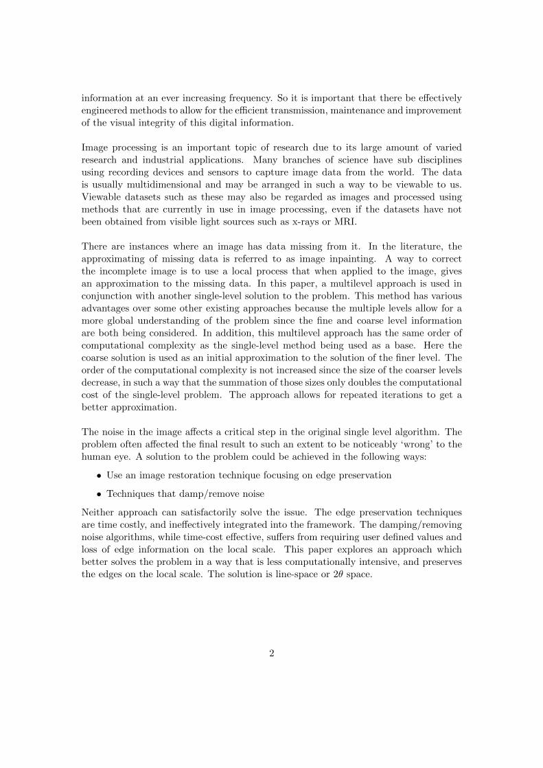
Figure 3: the importance of the filling order when dealing with concave target regions. (a)A diagram showing an image and a selected target (in white). The remainder of the image isthe source. (b,c,d) Different stages in the concentric-layer filling of the target region. (d) Theonion-peel approach produces artifacts in the synthesized horizontal structure (b’, c’, d’) Fillingthe target region by an edge-driven filling order achieves the desired artifact-free reconstruction.(d’) the final edge-driven reconstruction, where the boundary between the two background imageregions has been reconstructed correctly. Image courtesy of [12]

A problem that was encountered in this multigrid setup was how the interpolation of themask region from level to level was to be handled. Gazit [20] avoided this by using levelsof the same size which meant the mask did not change between levels. However, in thisframework, the size of the mask does not half in each dimension in relation to the griddimensions, as the problem is moved to the coarser grid. Since the mask is unknown, thepixels that belong to it propagate more unknown regions downwards to the coarser level.This means that the number of levels in the V-cycle is restricted by the growth of themask. Should the mask cover the vast majority of a level then patch-based inpaintingwill poorly fill the region, because of the lack of matching patches to choose from. Thisproblem is countered by restricting the number of coarser levels in the V-cycle. Multigridsmoothing (the error is being smoothed) is not used because there is no correct solutionto achieve. The completion algorithm Criminisi() in its altered form takes the placeof the smoothing methods in a V-cycle. The completion algorithm is slightly altered intwo ways from [12]. The modifications are aimed to slightly improve one part of thealgorithm and to allow for the inclusion of the data from previous iterations.

The completion method of [12] is characterized by the order in which to fill in themissing region and a similarity measure which determines what data will be used in the

14

Figure 4: Notation diagram. Given the patch Ψp. np is the normal to the contour δΩof the target region Ω and ∇I⊥p is the isophote (direction and intensity) at point p. theentire image is denoted with I. Image courtesy of [12]

patch. The authors of [12] showed that the order of completion affects how natural acompletion may be. A good comparison can be found in Figure 3.

The two alterations to the algorithm in [12] are small in nature. The authors of [12]chose their data term by calculating the gradient of all pixels located within the targetpatch and then chose the gradient with the maximum magnitude to be representativeof the central pixel. This means that multiple patches may have the same gradientsince the same maximum magnitude gradient pixel may be located within several targetpatches. The modification is to multiply the gradient magnitude of the pixels by theinverse of their distance from the center of the target patch. This means that the targetpatch whose center is closest to the maximum gradient has a larger data term thanits immediate neighbours. The second alteration is to the similarity measure, which isdescribed first.

11.1 Similarity Measure

The completion algorithm requires that target patches are filled in with texture, in theform of patches, from the known data of the image. This can be done in several waysand the authors of [12] used one of the more common measures. The unknown pixels inthe target patch are replaced by pixels from a source patch. The source patch is selectedby it having the smallest deviation between itself and the target patch. The deviation isdefined as the square of the difference in colour values of the known pixels in the target

15

patch and the known pixels in the source patch. This is then normalized by the numberof known pixels in the target patch. For a source patch S(p) the deviation is defined as:

1

|p|∑

(pk − S(pk))2

This is essentially the mean square error between the known pixels in the target patchand the pixels of the source patch in the same relative position within the patch as thetarget patch. The alteration is to have the mean square error over all the pixels in thetarget patch and source patch. This is because there is already an approximation tothe solution in the missing data (But the very first approximation has no values in themissing region). Including the approximations allow the iterations to improve the imageiteratively.

11.2 Computational Complexity

Although it may seem that using multiple images multiplies the cost of the entirecompletion, the implementation presented in this paper does not increase the complexityof the single-level completion algorithm [12]. This is because of the way in which thesmaller images in the V-cycle are created. As in multigrid for PDEs, the next grid issmaller by a factor of two for every dimension of the domain, for images that means thenext smaller image is one quarter the size. Each level, or smaller image, also uses thecompletion algorithm. Say that the completion algorithm has computational complexityof O(mn log n) where n is the number of pixels in the image and m is the number ofpatches needed to approximate the missing data. The log(n) comes from using FastFourier Transforms (FFTs) to calculate deviation between patches. Then summation ofeach level gives:

mn log(n) +mn log(n/4)/4 +mn log(n/16)/16 +mn log(n/64)/64 + . . .

<= mn log(n)(1 + 1/4 + 1/16 + 1/64 + . . . )

= mn log(n)(4/3)

Therefore, the cost of a V-cycle will only be a constant multiplied by the computationalcost of the algorithm of [12], and the algorithm presented in this paper is alsoO(mn log(n)).Since stopping criteria is not guaranteed for the iterations, an arbitrary constant (k)should be used for the number of iterations then the order of the algorithm isO(kmn log(n)).It should also be noted that the multiple levels are restricted to ones whose size is greaterthan the user defined size of a patch.

12 Results

The algorithm presented in this paper was tested on both synthetic and natural imagesthat were not chosen because they had the best results. They were chosen to illustrate

16

what the algorithm achieved over the single-level method [12] and what problems wereencountered for both. All approximations in the V-cycle column were achieved with nomore than 4 V-cycles.

13 Conclusion

This paper introduces a new concept to textured patching in image inpainting. Theability to repeatedly iterate an approximation while retaining the texture that is patchedin. This was done by using a framework of multilevel approaches with its origins insolving elliptic PDEs. By using this multilevel framework in conjunction with a welldevised texture patching method, it allows global structures to affect the local areaaround the missing data, instead of only using data from its local neighbours. Resultsof experiments vary but they appear to always be at least as good as the single-levelmethod, and without incurring any additional computational complexity.

14 Future Research

There seem to be three areas where the method presented in this paper may be improved.When interpolating from a small image to a large image perhaps a transition which takesinto account both images simultaneously would produce far less blur in the larger imageon the damped update of a V-cycle.

Another area of future research would be to change the similarity measure because”mean-square error is a poor indicator of texture matching and also of gradient matching.Entropy or variance may be considered as alternatives” [26]. Changing this may lead tobeing able to remove the multilevel framework completely and only using the single-levelmethod described in [12].

Another similarity measure [26] which has been shown to work very well is the StructuralSimilarity Index Measure (SSIM). It does however have a complexity cost at leastone order of magnitude greater than MSE. To get around this the SSIM could beinterspersed with MSE to reduce runtime but alternating between the two measures withany frequency will still increase the computational complexity of the original algorithm.

It could also be argued that the method in which the data-term is calculated may beimproved by a more accurate reading of structure, because as can be seen in Figure 5 itfocuses only on large magnitude changes instead of actual structure. In Figure 5 it canbe seen that the line is a horizontal one and all the other lines are textures, but againthis is quite difficult to describe to a computer. Altering the work done in [6] may lead

17

Original Image Image with Mask Criminisi Method V-cycle

the right side of theimage has artifacts

On both sides ofthe diagonal thereare noticeableartifacts

Below the diagonalthere appears to bea large artifact

Figure 5: Here is a comparison between the Criminisi method and the method proposedin this paper on several artificial images.

18

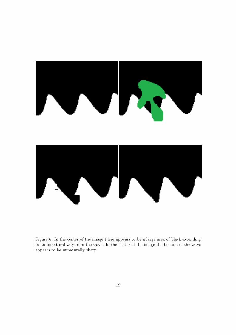
Figure 6: In the center of the image there appears to be a large area of black extendingin an unnatural way from the wave. In the center of the image the bottom of the waveappears to be unnaturally sharp.

19

Original Image Image with Mask Criminisi Method V-cycle

the algorithmjust missed fillingin the regioncorrectly butnot significantlyunnatural.

Here the patternis obvious to thehuman brain butboth methods failto capture thisaspect.

the horizontalextension fromthe bottom of thevisible textureappears distinctfrom the rest of theimage.

the center of theimage was notapproximated wellenough to capturethe aspects of theoriginal image.

Both methods failto completelyrestore theimage but theydo not addany ‘unnatural’artifacts.

Figure 7: Experimental Results (part 2)

20

Figure 8: Top-Left: original image. Top-Right: Image with Mask. Bottom-Left:Criminisi Method. Bottom-Right: V-cycle. Both methods fail to distinguish texturefrom structure resulting in poor completions of the image.

21

Figure 9: Top-Left: original image. Top-Right: Image with Mask. Bottom-Left: CriminisiMethod. Bottom-Right: V-cycle. This image has two very distinct edges extending into themissing region. Looking at in a linear structure sense, there does not appear to be a preference ifgrass is over the top of the pole or the other way around. Noticeable artifacts have appeared inthe missing region making the whole scene appear inconsistent. The pole had begun to extendupwards through the grass and the edge of the grass and the road was connected through themask.

22

Figure 10: Top-Left: original image. Top-Right: Image with Mask. Bottom-Left:Criminisi Method. Bottom-Right: V-cycle. Parts inside the triangle were filledincorrectly. The top of the triangle is slightly lopsided.

23

Figure 11: Top-Left: original image. Top-Right: Image with Mask. Bottom-Left:Criminisi Method. Bottom-Right: V-cycle. Parts from the border were included inthe missing region. The approximation seems slightly smooth on close inspection.

24

Figure 12: Top-Left: original image. Top-Right: Image with Mask. Bottom-Left:Criminisi Method. Bottom-Right: V-cycle. Another eye was replicated in the Criminisisolution above and left of her right eye. In the V-cycle solution the approximationappears blurry

25

to better results for capturing the structures.

It should be said that all areas of the algorithm may benefit from further research,such as edge-preserving interpolation or the stopping criteria. Perhaps the use of FullMultigrid (FMG) would be preferable to V-cycles.

Another improvement would be to calculate the isophotes using a method which averagesthe directions within a moving window to provide a better estimate of the data-termin the Criminisi algorithm. Currently I have a method which I have labeled 2θ. It is atransform which allows the addition of vectors in a constructive manner when the vectorslie along similar lines. In 2θ lines become vectors in a simplistic sense. In Euclideanspace, if a vector is added to a negative version of itself, it disappears which makes senseif it is worded as a vector minus itself. In 2θ-space these two concepts are different. In2θ-space lines are the new vectors. An important distinction between lines and vectorsis that lines have two opposite directions, so reversing the line returns itself. So adding anegative version of a line to itself should just yield the line back again. In this new space,if you add a perpendicular line to itself it results in nothing. This is the basic conceptfor 2θ-space. It is not rigorous in the sense of an actual space. It is more of an ideaof how to perform basic operations on vectors that result in a more line friendly approach.

This 2θ-space is well suited to multiple colour channels as well. Let us set up thecase where an image consists of 3 colour channels, so say red(R), green(G), blue(B).They correspond to the functions f , g, and h respectively. Each pixel in the imagehas a corresponding position in the domain, say (x, y) so we have the image beingf(x, y), g(x, y), h(x, y). Now the setup is that we are performing a moving windowaverage over an entire image for the purpose of extending structures linearly into amask inside the image. However let us focus on just an average of a small window onthe edge of the mask. As we see the image there are three clear isophotes in each of thecolour channels. If the isophote of f and g are perpendicular and of equal magnitudethen they would cancel each other out in 2θ-space, which is a benefit of this algorithmbecause the third function h has the isophote that decides the stalemate of the f andg interaction. Without loss of generality, if the isophote of h is strongly correlated to fthen the isophote is ’probably’ real and should be recorded as strong. If the isophoteis not strongly correlated with the ones from either f and g then the structure is nolonger linear and too complex to naturally extend into the mask. This type of action isstrongly suited for the algorithm of Criminisi.

Another direction that this research could take is moving from still images to sequencesof images which come under the heading of video processing. Adapting this algorithm forvideo can be done in a number of ways. We could treat each frame as a separate imageand run the algorithm, but this does not take advantage of the information availablein the image ahead and behind the current image. By using multiple images fromthe sequence, there is more data that can be used when inpainting the mask. I have

26

constructed a multigrid framework for still images which shows that this approach doeswork. There needs to be a consistency between consecutive completed images so thatthe linear structures extend in to the missing region is consistent across all frames. Thismeans more image processing techniques such as image registration and motion trackingmay have to be investigated to be employed because although there is only a shortinterval in the time between frames, the scene will generally change.

A real world example of this is close-up time-lapse photography of a flower in bloom.Usually since flowers reproduce in some way with pollen it attracts various insects ontothe petals for a short period of time. This means that there are insects appearing anddisappearing from frame to frame as the video runs. These insects are not a desirablepart of the video, if capturing the flower blooming is the purpose. Even in time-lapsethe image of the flower does not change drastically from one frame to the next, butperhaps the insect that was captured in one frame has disappeared in the next. Usinginformation from frames ahead and behind the current frame will help to effectivelyinpaint the mask better than using information from the surrounding area of the mask.In just this example of time-lapse photography there are many undesirable objects suchas water droplets or shadows. Time-lapse photography is generally used to capturescenes that humans understand better when viewed over a shorter period of time. Theidea is to capture events that are happening over a long period of time and not theevents in a short time frame. Eliminating the short time events is desirable in the worldof photography.

Another example of integrating this research into video processing would be to removean object that appears in multiple frames entirely from the video. Perhaps there issomething going on in the background that detracts from the visual appeal of videoand the background event needs to be removed. As long as the background event isproperly identified over the sequence of images, the mask can be inpainted properlyand the algorithm would definitely benefit from having the information from multipleframes. This can be understood most easily when considering a motionless camera. Byjust averaging all the frames you cancel out moving objects because as the objects movethey reveal the true information that was hidden behind them. By taking this approachit may be possible to correctly restore the video to match the physical scene it wascapturing. Whereas in image processing the information behind the mask is not knownnor can it be determined exactly from the rest of the image. Video processing mayintroduce another dimension into the problem but it also introduces new informationwith meaningful consequences.

Bibliography

[1] John Aloimonos. Shape from texture. Biological cybernetics, 58(5):345–360, 1988.

27

[2] M. Ashikhmin. Synthesizing natural textures. In Proceedings of the 2001 Symposiumon Interactive 3D Graphics, pages 217–226, New York, NY, USA, 2001. ACM Press.

[3] Ziv Bar-joseph, Ran El-Yaniv, Dani Lischinski, and Michael Werman. Texturemixing and texture movie synthesis using statistical learning. IEEE Transactionson Visualization and Computer Graphics, 7:120–135, 2001.

[4] Marcelo Bertalmıo, Guillermo Sapiro, Vicent Caselles, and Coloma Ballester. Imageinpainting. In SIGGRAPH, pages 417–424, 2000.

[5] Marcelo Bertalmio, Guillermo Sapiro, Vincent Caselles, and Coloma Ballester.Image inpainting. In Proceedings of the 27th annual conference on Computergraphics and interactive techniques, pages 417–424. ACM Press/Addison-WesleyPublishing Co., 2000.

[6] Marcelo Bertalmio, Luminita Vese, Guillermo Sapiro, and Stanley Osher.Simultaneous structure and texture image inpainting. In IEEE Transactions onImage Processing, volume 12, pages 882–889, August 2003.

[7] Jose M Bioucas-Dias, Mario AT Figueiredo, and Joao P Oliveira. Totalvariation-based image deconvolution: a majorization-minimization approach. InAcoustics, Speech and Signal Processing, 2006. ICASSP 2006 Proceedings. 2006IEEE International Conference on, volume 2, pages II–II. IEEE, 2006.

[8] Andrew Blake and Constantinos Marinos. Shape from texture: estimation, isotropyand moments. Artificial Intelligence, 45(3):323–380, 1990.

[9] Jeremy S. De Bonet. Multiresolution sampling procedure for analysis and synthesisof texture images. In SIGGRAPH, pages 361–368, 1997.

[10] Richard J Cant and Carol S Langensiepen. A multiscale method for automatedinpainting. In 17th European Simulation Multiconference, pages 148–153, 2003.

[11] T Chan and J Shen. Non-texture inpaintings by curvature-driven diffusions. Journalof Visual Communication and Image Representation, 12(4):436–449, 2001.

[12] Antonio Criminisi, Patrick Perez, and Kentaro Toyama. Region filling andobject removal by exemplar-based image inpainting. IEEE Transactions on ImageProcessing, 13(9):1200–1212, 2004.

[13] Antonio Criminisi, Patrick Perez, and Kentaro Toyama. Region filling and objectremoval by exemplar-based image inpainting. Image Processing, IEEE Transactionson, 13(9):1200–1212, 2004.

[14] Alexei A. Efros and William T. Freeman. Image quilting for texture synthesis andtransfer. In SIGGRAPH, pages 341–346, 2001.

[15] Alexei A. Efros and Thomas K. Leung. Texture synthesis by non-parametricsampling. In ICCV, pages 1033–1038, 1999.

28

[16] Alexei A Efros and Thomas K Leung. Texture synthesis by non-parametricsampling. In Computer Vision, 1999. The Proceedings of the Seventh IEEEInternational Conference on, volume 2, pages 1033–1038. IEEE, 1999.

[17] Pedro F Felzenszwalb and Daniel P Huttenlocher. Efficient belief propagation forearly vision. International journal of computer vision, 70(1):41–54, 2006.

[18] Michal Holtzman Gazit. Multi Level Methods for Data Completion. PhD thesis,Israel Institute of Technology, 2010.

[19] Paul Harrison. A non-hierarchical procedure for re-synthesis of complex textures.In WSCG, pages 190–197, 2001.

[20] Michal Holtzman-Gatiz and Irad Yavneh. A scale-consistent approach to imagecompletion. International Journal for Multiscale Computational Engineering,6(6):617–628, 2008.

[21] Kenichi Kanatani. Shape from Texture. Springer, 1990.

[22] Vivek Kwatra, Arno Schodl, Irfan A. Essa, Greg Turk, and Aaron F. Bobick.Graphcut textures: image and video synthesis using graph cuts. ACM Trans.Graph., 22(3):277–286, 2003.

[23] Andrei Rares, Marcel J. T. Reinders, and Jan Biemond. Edge-based imagerestoration. IEEE Transactions on Image Processing, 14(10):1454–1468, 2005.

[24] T.K. Shih, Liang-Chen Lu, Ying-Hong Wang, and Rong-Chi Chang.Multi-resolution image inpainting. In 2003 International Conference on Multimediaand Expo, volume 1, pages I–485–8 vol.1, 2003.

[25] Jian Sun, Lu Yuan, Jiaya Jia, and Heung-Yeung Shum. Image completion withstructure propagation. ACM Trans. Graph., 24(3):861–868, 2005.

[26] Zhou Wang, Alan C Bovik, Hamid R Sheikh, and Eero P Simoncelli. Image qualityassessment: from error visibility to structural similarity. Image Processing, IEEETransactions on, 13(4):600–612, 2004.

[27] Li-Yi Wei and Marc Levoy. Fast texture synthesis using tree-structured vectorquantization. In SIGGRAPH, pages 479–488, 2000.

29