Image Gradient Based Level Set Methods in 2D and 3Dcsjason/papers/xxetal.pdfImage Gradient Based Level Set Methods in 2D and 3D Xianghua Xie, Si Yong Yeo, Majid Mirmehdi, Igor Sazonov,

Image Gradient Based Level Set Methods in 2Dand 3D

Xianghua Xie, Si Yong Yeo, Majid Mirmehdi, Igor Sazonov, and PerumalNithiarasu

Abstract This chapter presents an image gradient based approach to perform 2Dand 3D deformable model segmentation using level set. The 2D method uses anexternal force field that is based on magnetostatics and hypothesized magnetic in-teractions between the active contour and object boundaries. The major contributionof the method is that the interaction of its forces can greatly improve the active con-tour in capturing complex geometries and dealing with difficult initializations, weakedges and broken boundaries. This method is then generalized to 3D by reformulat-ing its external force based on geometrical interactions between the relative geome-tries of the deformable model and the object boundary characterized by image gra-dient. The evolution of the deformable model is solved using the level set method sothat topological changes are handled automatically. The relative geometrical config-urations between the deformable model and the object boundaries contribute to a dy-namic vector force field that changes accordingly as the deformable model evolves.The geometrically induced dynamic interaction force has been shown to greatlyimprove the deformable model performance in acquiring complex geometries andhighly concave boundaries, and it gives the deformable model a high invariancy ininitialization configurations. The voxel interactions across the whole image domainprovide a global view of the object boundary representation, giving the externalforce a long attraction range. The bidirectionality of the external force field allowsthe new deformable model to deal with arbitrary cross-boundary initializations, andfacilitates the handling of weak edges and broken boundaries.

Xianghua XieSwansea University, Department of Computer Science, Faraday Tower, Singleton Park, SwanseaSA2 8PP, United Kingdom, e-mail: [email protected]

Majid MirmehdiBristol University, Department of Computer Science, Merchant Ventures Building, Bristol BS81UB, United Kingdom, e-mail: [email protected]

Si Yong Yeo, Igor Sazonov and Perumal NithiarasuSwansea University, College of Engineering, Talbot Building, Singleton Park, Swansea SA2 8PP,United Kingdom.

1

2 Xianghua Xie, Si Yong Yeo, Majid Mirmehdi, Igor Sazonov, and Perumal Nithiarasu

1 Introduction

Depending on the assumption of how object boundary is described, active con-tours can be classified into edge based [Caselles et al(1997)Caselles, Kimmel, andSapiro, Xu and Prince(1998), Paragios et al(2004)Paragios, Mellina-Gottardo, andRamesh, Li et al(2005)Li, Liu, and Fox], region based [Chan and Vese(2001), Para-gios and Deriche(2002), Cremers et al(2007)Cremers, Rousson, and Deriche], andhybrid approaches [Haddon and Boyce(1990),Chakraborty et al(1996)Chakraborty,Staib, and Duncan, Xie and Mirmehdi(2004)]. For edge based methods, it is as-sumed that object boundaries collocate with image intensity discontinuities whichis widely adopted, for example, in depth estimation from stereo [Birchfield andTomasi(1999)]. Region based techniques, on the other hand, assume that objectboundaries collocate with discontinuities in regional characteristics, such as colorand texture. In other words, each object has its own distinctive and continuous re-gional features.

Region based techniques have some obvious advantages over edge based meth-ods in that object boundary description based on image gradient can often be com-promised by noise and weak edges. They are also less sensitive to initialization,while edge based active contours are prone to local minima. Thus, it is often de-sirable for edge based techniques to carefully place the initial contour. This as-sumes that the prior knowledge of the object location is available, which is notalways true in reality. Existing techniques can only reduce this initialization de-pendency to a very limited extent. The balloon force [Caselles et al(1997)Caselles,Kimmel, and Sapiro] can only expand or shrink the contours. The bidirectional-ity of GVF can sometimes cause the contours to collapse on approach to the sameboundary. Moreover, it has convergence issues caused by critical points. [Gil andRadeva(2003), Paragios et al(2004)Paragios, Mellina-Gottardo, and Ramesh, Xieand Mirmehdi(2008)]. It is evidently clear that initialization invariance is partic-ularly difficult to achieve for edge based methods. More recent attempts, suchas [Gil and Radeva(2003), Paragios et al(2004)Paragios, Mellina-Gottardo, andRamesh,Jalba et al(2004)Jalba, Wilkinson, and Roerdink,Li et al(2005)Li, Liu, andFox], showed promising but limited success.

In this chapter, we present an image gradient based approach to perform 2Dand 3D deformable model segmentation using level set. Section 2 presents the2D method which uses an external force field that is based on magnetostatics andhypothesized magnetic interactions between the active contour and object bound-aries. The major contribution of the method is that the interaction of its forces cangreatly improve the active contour in capturing complex geometries and dealingwith difficult initializations, weak edges and broken boundaries. This method isthen generalized to 3D in Section 3 by reformulating its external force based ongeometrical interactions between the relative geometries of the deformable modeland the object boundary characterized by image gradient. The relative geometricalconfigurations between the deformable model and the object boundaries contributeto a dynamic vector force field that changes accordingly as the deformable modelevolves. Experimental results are shown in Section 4. The proposed dynamic inter-

X. Xie et al. Image Gradient Based Level Set Methods in 2D and 3D 3

action force has been shown to greatly improve the deformable model performancein acquiring complex geometries and highly concave boundaries, and it gives thedeformable model a high invariancy in initialization configurations. The voxel inter-actions across the whole image domain provide a global view of the object boundaryrepresentation, giving the external force a long attraction range. The bidirectionalityof the external force field allows the new deformable model to deal with arbitrarycross-boundary initializations, and facilitates the handling of weak edges and brokenboundaries.

2 MAC model: a 2D approach

Fittings based on local intensity discontinuity can often lead to undesired local min-ima. The CPM [Jalba et al(2004)Jalba, Wilkinson, and Roerdink] assigns oppositecharges to edges and free particles so that the particles are pulled towards edgeswhile repelling each other. This global interaction provides much freedom of ini-tialization. However, particles on weak edge can be gradually pulled towards neigh-boring strong edges, resulting in broken boundaries. Particle addition and deletionand contour reconstruction can also be difficult in practice.

Instead of assigning fixed charges, we allow the charges flow through the edges.These flows of charges will then generate a magnetic field. The active contour, car-rying similar flow of charges, will be attracted towards the edges under this magneticinfluence. Without losing generality, let us consider the image plane as a 2D planein a 3D space whose origin coincides with the origin of the image coordinates. Ad-ditionally, the third dimension of this 3D space is considered perpendicular to theimage plane.

The direction of the currents, flows of charges, running through object boundarycan be estimated based on edge orientation, which can be conveniently obtained bya 90 rotation in the image plane of the normalized gradient vectors (Ix, Iy), where Idenotes an image. Let x denote a point in the image domain. Thus, the object bound-ary current direction, O(x), can be estimated as: O(x) = (−1)λ (−Iy(x), Ix(x),0),where λ = 1 gives an anti-clockwise rotation in the image coordinates, and λ = 2provides a clockwise rotation. However, we show later by using the proposed levelset updating scheme different λ values lead to the same result. Since the activecontour is embedded in a signed distance function, the direction of current for thecontour, denoted as υ , can be similarly obtained by rotating the gradient vector ∇Φof the level set function. Similar to O, υ is also three dimensional and lies in theimage domain, i.e. υ(x) = (−Φy(x),Φx(x),0).

Let f (x) be the magnitude of edge pixel and the magnitude of boundary currentbe proportional to edge strength, that is, the electric current on object boundary isdefined as f (x)O(x). The magnetic flux B(x) generated by gradient vectors at eachpixel position x can then be computed as:


B(x) ∝ ∑s∈S,s =x

f (s)O(s)× Rxs

R2xs, (1)

where s denotes an edge pixel position, S is the set containing all the edge pixel po-sitions across the image, Rxs denotes a 3D unit vector from x to s in the image plane,and Rxs is the distance between them. Thresholding can be applied to remove someerroneous edge pixels with very small gradient magnitude [Jalba et al(2004)Jalba,Wilkinson, and Roerdink,Xie and Mirmehdi(2008)]. The active contour is assignedwith unit magnitude of electric current. The force imposed on it can be derived as:

F(x) ∝ υ(x)×B(x). (2)

From (1) and (2), we can see that B intersects the image plane perpendicularly andF is always perpendicular to both υ and B. Thus, F also lies in the image domainand its third element equals to zero. For simplicity, from now on, we shall ignoreits third dimensional component and denote F(x) as a 2D vector field in the imagedomain. The basic model can then be formulated as:

dCdt

= αg(x)κn+(1−α)(F(x) · n)n, (3)

where g(x) = 1/(1+ f (x)), κ denotes the curvature, and n is inward unit normal.Its level set representation then takes this form:

∂Φ∂ t

= αg(x)∇ ·(

∇Φ|∇Φ |

)|∇Φ |− (1−α)F(x) ·∇Φ . (4)

We can see from (1) and (2) that the image force is derived from global inter-actions among rotated gradient vectors, i.e. f (x)O(x). Thus, it is more robust thanfittings based on local gradient towards weak edges (where f (x) is small) and noise(where O(x) is locally inconsistent). It is worth noting, however, that general con-trast consistency along the object boundaries is important to the model. Large con-trast variation can disrupt the force field, e.g. half of the object appears brighter thanbackground and the other half appears to be darker. However, this does not meanthat the entire object has to be brighter or darker than background. Those regionsaway from object boundary can be continuously varying in intensity. The modelalso can tolerate a fair amount of local contrast inconsistency, in the same way as toimage noise and weak/broken edges.

As aforementioned, due to cross product computation the external force, F, isalways perpendicular to υ which is tangent to the contour, i.e. the external force isimposed along the normal direction. Note the internal force due to curvature flowis enforced in the inward normal direction. Thus, the total force is always perpen-dicular to active contour. In other words, it dynamically updates itself accordingto contour evolution to push and pull the contours along the normal direction untilthey reach object boundaries where forces from both sides are in balance. As a re-sult, the propagating contour will not suffer from those convergence issues related to


static force fields, such as GVF, in which evolving contours may become tangent tounderlying force vectors resulting in false convergence. This force field is also sig-nificantly different from others used in edge based methods. For example, in CPM,the force between an edge pixel s and an infinitesimal contour segment c lies in astraight line between these two, regardless the orientation of the contour segment.In our model, the orientation of the edge pixel and the contour segment also haveinfluence on the resulting force interaction. This ability to adapt is very importantsince it ensures the active contour, once initialized, overcome deep concavities andnarrow regions to reach object boundaries.

O

C1

FF

(A)

C2

O

C1

C2

F F

(B)

O

C1

F

(C)

C3

F

C2

F

C1

C2

F F

O

(D)

Fig. 1 Preventing contour collapsing. (a): Two contours, C1 and C2, are placed on each side of anobject boundary with current directions indicated by arrows. Contour C1 is attracted by the objectboundary and expands itself in the outward normal direction. It eventually will wrap around andcapture the object boundary. Contour C2 however is repelled and forced to shrink in the inwardnormal direction. Thus, two contours will not collapse to each other. (b): Similar to (a), howevercontour C1 is placed across the object boundary. Those contour segments of C1 that are insideobject boundary will be pulled towards object boundary and the rest of contour C1 will expandand wrap around the object boundary. The segments inside object boundary and outside will notcollapse to each other. (c): The object in this case contains an internal boundary. The behavior ofC1 and C2 is similar to that in (a). Contour C3 will expand itself to capture the internal boundary.Three contours will not collapse to each other, while capturing both boundaries. (d): Contours C1and C2 are now initialized across external and internal boundaries, respectively. The behavior ofC1 is similar to that in (b). The contour segments of C2 that are inside the object (gray area) willbe attracted to the object internal boundary that is initially inside contour C2. The other contoursegments of C2 will expand to capture the rest internal boundaries. No contour collapsing willoccur, either. GVF contours, as an example, will collapse to each other in all above scenarios.

By incorporating (2), Eqn. (3) can be re-written as:

dCdt

= αg(x)κn+(1−α)(υ(x)×B(x) · (n,0)) n (5)

= αg(x)κn+(1−α)(B(x) · ((n,0)×υ(x))) n.


The external force in the second term is in fact a projection of the magnetic fluxonto a binormal unit vector which is computed from a cross product of the contourinward normal and its tangent vector. A positive projection will force the contourto expand and a negative projection will shrink the contour, which acts in a similarway as what a region indication function does in a region based approach, however,this is derived from the edge based assumption. Thus, an edge can attract or pusha contour which may lie either side of the edge. However, this bidirectionality isfundamentally different from that in, for example, GVF. In GVF, the force imposedon the contour is independent of the contour itself, which can cause the contours tocollapse to each other when reaching to the same object boundary. For the proposedmethod, the force is related to both the image gradient and the contour (which canbe clearly seen from Eqn. (5)). It has the ability to prevent the contour from reachingto the same boundary and disappearing after merging together.

In [Xie and Mirmehdi(2008)], we proposed to perform nonlinear diffusion of themagnetic field in order to overcome noise interference when necessary. An edgesaliency measure can be added to the weighting function in order to better preservethe edges [Xie(2010)]. Let B(x) denote the signed magnitude of B(x). The diffusedfield B(x) is obtained by solving:

dB

dt(x) = p(B(x))∇2B(x)−q(B(x))(B(x)−B(x)), (6)

where p(B(x)) = e−|B(x)|S (x)

K , q(.) = 1− p(.), and S (.) is an edge saliency measurewhich is measured based on edge strength and orientation coherency, i.e. S (x) =f (x)v(x) where v(.) is the variance of orientation in a local neighborhood, e.g. 9×9as used here. More sophisticated saliency measures, e.g. [Heidemann(2005)], canbe used. Weighting the flux magnitude with S (.) further ensures as little diffusionas possible at object boundaries, while areas lack of consistent support from edgesresult in substantial diffusion.

3 Extenstion to 3D

Shape segmentation from volumetric data has an important role in applications suchas medical image analysis. Volumetric image segmentation remains an intricate pro-cess, due to the complexity and variability of image data and shapes (i.e. anatomicalstructures). There have been applications of simple techniques such as thresholdingand region growing in the extraction of 3D objects from volumetric images [Smithet al(2007)Smith, Smith, Williams, Rodriguez, and Hoying, Wu et al(2008)Wu, Ye,Ma, Sun, Xu, and Cui]. However, these techniques are very sensitive to noise and in-tensity inhomogeneities which exist in real images, and often produce leakages andregions which are not contiguous. Statistical approaches [Ruan et al(2000)Ruan,Jaggi, Xue, Fadili, and Bloyet, Hao and Li(2007)] are also used to identify differ-ent tissue structures from medical images. It usually involves manual interaction


to segment images in order to obtain a sufficiently large set of training samples.Such strategies are often restricted to problems where there is sufficient prior knowl-edge about the shape or appearance variations of the relevant structures. Also, theuse of the same training set for a large number of image scans may lead to bi-ased results that do not take sufficient consideration of the variability within indi-viduals. Atlas based approaches perform segmentation based on image registrationtechniques [Maintz and Viergever(1998)], whereby an image can be segmented byfinding a transformation that maps a template image to the target image. It is how-ever generally difficult for atlas based techniques to accurately extract complex ge-ometries such as those from volumetric medical images due to the variability ofanatomical structures.

The external force field presented previously is based on the hypothesized mag-netic force between the active contour and object boundaries. This formulation canbe applied directly in the magnetostatic active contour to compute the magneticfield and force required to draw the active contour towards object boundaries in2D images. This image gradient based method showed significant improvementson convergence issues, e.g. reaching deep concavities, and in handling weak edgesand broken boundaries. When applying the analogy directly to deformable model-ing, it requires estimation of tangent vectors for the deformable contours, which isconvenient in 2D case, however, not possible in 3D. Our approach is to define anovel external force field that is based on hypothesized geometrically induced in-teractions between the relative geometries of the deformable model and the objectboundaries (characterized by image gradients). In other words, the magnitude anddirection of the interaction forces are based on the relative position and orientationbetween the geometries of the deformable model and image object boundaries, andhence, it is called the geometric potential force (GPF) field [Yeo et al(2011)Yeo,Xie, Sazonov, and Nithiarasu]. The bidirectionality of the new external force fieldcan facilitate arbitrary cross-boundary initialization, which is a very useful feature tohave, especially in the segmentation of complex geometries in 3D. It also improvesthe performance of the deformable model in handling weak edges. In addition, theproposed external force field is dynamic in nature as it changes according to therelative position and orientation between the evolving deformable model and objectboundary. This GPF force however is in fact a 3D extension of the 2D MAC model.

t^ t'^n

n'

rdl

dl'xx'

C C'

n

n'

dA

dA'

x'

x

SS'

rxx'

Fig. 2 Relative position and orientation between geometries in 2D and 3D.


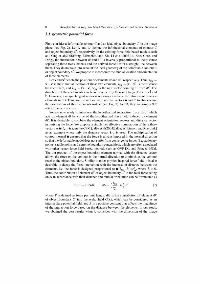
3.1 geometric potential force

First, consider a deformable contour C and an ideal object boundary C′ in the imageplane (see Fig. 2). Let dl and dl′ denote the infinitesimal elements of contour Cand object boundary C′, respectively. In the existing force field based models suchas [Yang et al(2006)Yang, Mirmehdi, and Xie, Li et al(2007)Li, Kao, Gore, andDing], the interaction between dl and dl′ is inversely proportional to the distanceseparating these two elements and the derived force lies in a straight line betweenthem. They do not take into account the local geometry of the deformable contour Cor object boundary C′. We propose to incorporate the mutual location and orientationof these elements.

Let x and x′ denote the positions of elements dl and dl′, respectively. Thus, rxx′ =x− x′ is their mutual location of those two elements, rxx′ = |x− x′| is the distancebetween them, and rxx′ = (x− x′)/rxx′ is the unit vector pointing dl from dl′. Thedirections of these elements can be represented by their unit tangent vectors t andt′. However, a unique tangent vector is no longer available for infinitesimal surfaceelements in 3D. Thus, we use unit outward normal vectors n and n′ to characterizethe orientations of these elements instead (see Fig. 2). In 2D, they are simply 90

rotated tangent vectors.We are now ready to introduce the hypothesized interaction force dFdl which

acts on element dl by virtue of the hypothesized force field induced by elementdl′. It is desirable to combine the element orientation vectors and distance vectorin deriving the force. We propose a simple but effective combination of these threevectors as n(rxx′ ·n′), unlike CPM [Jalba et al(2004)Jalba, Wilkinson, and Roerdink]as an example where only the distance vector rxx′ is used. The multiplication ofcontour normal n ensures that the force is always imposed in the normal directionso that the deformable model does not suffer from convergence issues (i.e. stationarypoints, saddle points and extreme boundary concavities), which are often associatedwith other vector force field based methods such as GVF [Xu and Prince(1998)].The dot product of the object boundary element normal with the distance vectorallows the force on the contour in the normal direction to diminish as the contourreaches the object boundary. Similar to other physics-inspired force field, it is alsodesirable to decay the force interaction with the increase of distance between theelements, i.e. the force is designed proportional to n(rxx′ · n′)/rλ

xx′ where λ > 0.Thus, the contribution of element dl′ of object boundary C′ to the total force actingon dl in accordance with their distance and mutual orientation can be formulated as

dFdl = ndGdl, dG =( rxx′

rλxx′

· n′)

dl′ (7)

where F is defined as force per unit length, dG is the contribution of element dl′

of object boundary C′ into the scalar field G(x), which can be considered as anintermediate potential field, and λ is a positive constant that affects the magnitudeof the interaction force based on the distance between the elements. In our study,we obtained the best results when λ coincides with the dimension of the image


data, i.e. λ = 2 in the 2D case. Furthermore, we show later that when λ coincideswith data dimension in 2D, the proposed force interaction has an explicit link to themagnetostatics theory and thus the spatial decay of the magnitude of the interactionforce is analogous to that of the magnetic field.

As shown in (7), the computation of the new force field only requires unit normalvectors and relative position of the two elements, which is convenient to acquire.Thus, this new force field can be easily extended to higher dimensions, e.g. 3D. LetdA belong to the deformable surface S whereas dA′ belongs to the object boundaryS′ (see Fig. 2). The generalized 3D version of force dFdA acting between these twoarea elements can be readily given as

dFdA = ndGdA, dG =( rxx′

rλxx′

· n′)

dA′ (8)

where F is defined as force per unit area, G is the corresponding 3D potential field,n and n′ are unit surface normals of the deformable model and object boundary,respectively, and λ = 3. Again, the magnitude and direction of the induced force F ishandled intrinsically by the relative position and orientation between the geometriesof the deformable model determined by the evolving surface S and object boundarydetermined by S′. Since the force is derived geometrically and its interaction is afunction of inverse distance, we name it geometric potential force (GPF).

3.2 GPF Deformable Model

The GPF force in (8) is derived using geometrical information from ideal objectboundaries. Next, we extend this to deal with real image data and formulate it in3D deformable modelling. In this work, we adopt an edge based approach, that isusing image intensity discontinuity to estimate the presence and strength of objectboundaries.

Let I(x) denote the 3D image, where x is a voxel location in the image domain.Temporarily, we consider x as a continuously varying point. One may treat this asan interpolation between voxel grid points to obtain a continuous image I(x). Tocompute the force acting on dA, we first compute the total potential field for anarbitrary point x:

G(x) = P.V. ∫∫S′

W (x′)( rxx′

rλxx′

· n′(x′))

dA′. (9)

where W (·) is a weighting function that is defined later, and P.V. means ‘PrincipalValue’: the contribution of infinitesimal circular vicinity of singular point x′ = x intothe integral is disregarded, which occurs when surfaces S and S′ intersect.

First, we consider the case, in which S′ can be defined rigorously on an idealobject O, i.e. S′ = ∂O. The object O can be specified by a binary image:


I (x) =

I0 x ∈ O0 x /∈ O,

(10)

where I0 is a nonzero constant. For such an image, ∇I is infinite on S′ and can berepresented through the 3D Dirac’s delta as

∇I (x) = ∆I δ (x−x′) n′(x′) (11)

where ∆I is the jump in function I (x) at the boundary of O; x′ ∈ S′ and n′(x′) isthe unit normal vector to the surface S′. Setting W equal to the jump of I at theboundary, i.e. W = ∆I , we can re-write (9) as a volume integral

G(x) = P.V.∫∫∫

Ω

W (x′)( rxx′′

rλxx′′

· n′(x′))

δ (x′′−x′)dV ′′ (12)

Here, x′′ is the integration variable and dV ′′ denotes a volume element. The Dirac’sdelta is used to obtain the area element from the volume element, i.e. dA′ → δ (x′′−x′)dV ′′.

Taking into account (11) and W =∆I , we can replace the product W (x′) n′(x′)δ (x′′−x′) in the integral of (12) by ∇I (x′′). Thus, (12) can be re-formulated as

G(x) = P.V.∫∫∫

Ω

( rxx′′

rλxx′′

·∇I (x′′))

dV ′′. (13)

It is now readily generalizable to real 3D data.In real images, ∇I is a smooth function reaching maximum magnitude in the

vicinity of the object boundary. The natural generalization of (13) is to substituteDirac’s delta by this smoothed function analog into (13), i.e. W (x′) n′(x′)δ (x′′ −x′)→ ∇I(x′′), where I denotes a real image. The geometric potential field in a con-tinuous form can then be formulated as

G(x) = P.V.∫∫∫

Ω

( rxx′

rλxx′

·∇I(x′))

dV ′. (14)

Note, due to the substitution of W (x′) n′(x′)δ (x′′ − x′) by ∇I(x′′), the x′ definedon the ideal surface S′ is no longer needed. Hence, the notation is simplified byreplacing the integral variable x′′ with x′. Finally, its discrete form can be written as

G(x) = ∑x′∈Ω ,x′ =x

( rxx′

rλxx′

·∇I(x′)). (15)

This can be considered as a convolution of the image gradient with the vector kernelKλ (x)

X. Xie et al. Image Gradient Based Level Set Methods in 2D and 3D 11Kλ (x) = P.V.

x|x|λ

= P.V.x|x|λ+1

G = Kλ ∗∇I =∫∫∫

Ω

(Kλ (x−x′) ·∇I(x′)

)dV ′

(16)

which can be computed efficiently using the fast Fourier transform (FFT). Note thatthe potential field G is computed as a convolution of two vector functions.

The total force acting on the unit area element of the deformable surface S isthus given as F = nG(x). where n is the outward unit normal of level set surface.Note, an inward normal can also be used, i.e. F =−nG(x), which will result in op-posite deformable model propagation since the force field is exactly in the oppositedirection. Hence, the force can be re-written in a generalized form:

F = J nG(x). (17)

where J is a constant taking values of ±1. Note this is different from the con-stant force in the geodesic model, where the force is monotonically expanding orshrinking. The sign convention ± is merely used to determine whether outward andinward normals of the deformable surface are considered.

The general contrast consistency along the object boundaries however is impor-tant to the model. Large contrast variation can disrupt the force field, e.g. half ofthe object appears brighter than background and the other half appears to be darker.However, this does not mean that the entire object has to be brighter or darker thanbackground. Those regions away from object boundary can be continuously varyingin intensity.

Once the force field F(x) is derived from the hypothesized interactions based onthe relative geometries of the deformable model and object boundary is determined,the evolution of the deformable model S(x, t) under this GPF field can be given as

dSdt

=(F · n

)n. (18)

Since surface smoothing is usually desirable, the mean curvature flow can be in-corporated and the complete GPF deformable model evolution can be formulatedas

dSdt

= α gκ n+(1−α)(F · n

)n (19)

where g(x) = 1/(1 + |∇I|) is the edge stopping function. Note that in our case,the flow of F is directed by definition normal to surface S, therefore

(F · n

)n = F.

Notation(F · n

)n is inherited from the traditional methods, e.g. GGVF. The level set

representation of the proposed deformable model based on GPF can then be writtenas

∂Φ∂ t

= α gκ |∇Φ |− (1−α)(F ·∇Φ) (20)

where Φ(t,x) is the level set function, such that the deformable surface S is definedas Φ(t,x) = 0. Note, the GPF force field is defined on the deformable surface, which


is implicitly embedded in the level set function, i.e. the force field computed at thepropagating front needs to be extended across the computational domain so that thefull level set function can be continuously evolved. Although direct force extensionmethod such as [Adalsteinsson and Sethian(1998)] can be used, we can convenientlycompute the GPF forces for each level set so that this external force is extended tothe entire level set function.

The GPF deformable model differs from conventional edge based models byutilizing edge voxel interactions across the whole image, thus providing a moreglobal view of the object boundary. The magnitude of the potential field strengthat each image location x is based on the relative position of x with all other voxelsin the image. Therefore, voxels at homogeneous regions will also have a non-zeropotential field strength. In this way, surfaces which are initialized far away fromobject boundaries can propagate towards the image edges and converge.

As shown in (8), the dot product rxx′ · n′ can be both positive and negative, de-pending on the relative configurations of the geometries between the deformablemodel and the image boundaries, thus giving a bidirectional vector force field. Thisuseful bidirectionality facilitates arbitrary cross boundary initializations, as its forcevectors point towards the object boundary from both ways. This also allows themodel to stabilize the deformable surfaces at weak edges, thus preventing leakage.

The physics-based deformable models described in [Li et al(2007)Li, Kao, Gore,and Ding, Jalba et al(2004)Jalba, Wilkinson, and Roerdink, Yang et al(2006)Yang,Mirmehdi, and Xie, Park and Chung(2002), Zhu et al(2008)Zhu, Zhang, Zeng, andWang] all use a kernel based function to compute the external force field with ker-nels being decreasing functions of distance from the origin. They are in effect equiv-alent to the external force derived in [Li et al(2007)Li, Kao, Gore, and Ding] basedon convolving a vector field with the edge map. For example, the external forcein [Jalba et al(2004)Jalba, Wilkinson, and Roerdink] can be represented as a convo-lution with the same kernel Kλ (16) with λ = 2:

Fa(x) =q

4πε(Kλ ∗ |∇I|

), Fr(x) =

q2

4πε(Kλ ∗1Ω

)(21)

where 1Ω (x) is a function equal to 1 when x ∈ Ω and 0 otherwise. The repellingforce is largely imposed in the tangential direction, which has very limited effect onchanging the shape or topology of the deformable model. Thus, it is not necessary inour model. In order to compare with the dominant attraction force Fa, we combine(16) and (17) and rewrite the GPF force as

FGPF = J n(Kλ ∗∇I

)(22)

It is clear that the GPF force is directed by the normal of the deformable model, i.e.it does not contain the tangential ‘parasitic’ component in contrast to the Fa force.Moreover, the proposed GPF takes into account edge orientations, as well as edgestrength (the convolution in (21) is based on a convolution of a vector function on ascalar field; whereas in (22) it is carried out on a vector field).


4 Experimental results

In this section, we present experimental results on both synthetic and real worldimage data. The comparative analysis is performed using several classical and state-of-the-art methods, which consists of image gradient based and region based meth-ods. In particular, the geodesic model is included as a representative of conven-tional local edge fitting based method which is based on monotonically expandingor shrinking force. The various vector field based models, such as [Li et al(2007)Li,Kao, Gore, and Ding, Jalba et al(2004)Jalba, Wilkinson, and Roerdink, Park andChung(2002),Zhu et al(2008)Zhu, Zhang, Zeng, and Wang], have very similar con-vergence and initialization dependence behavior to the GVF or GGVF, since theirdominant external forces are static as discussed earlier.

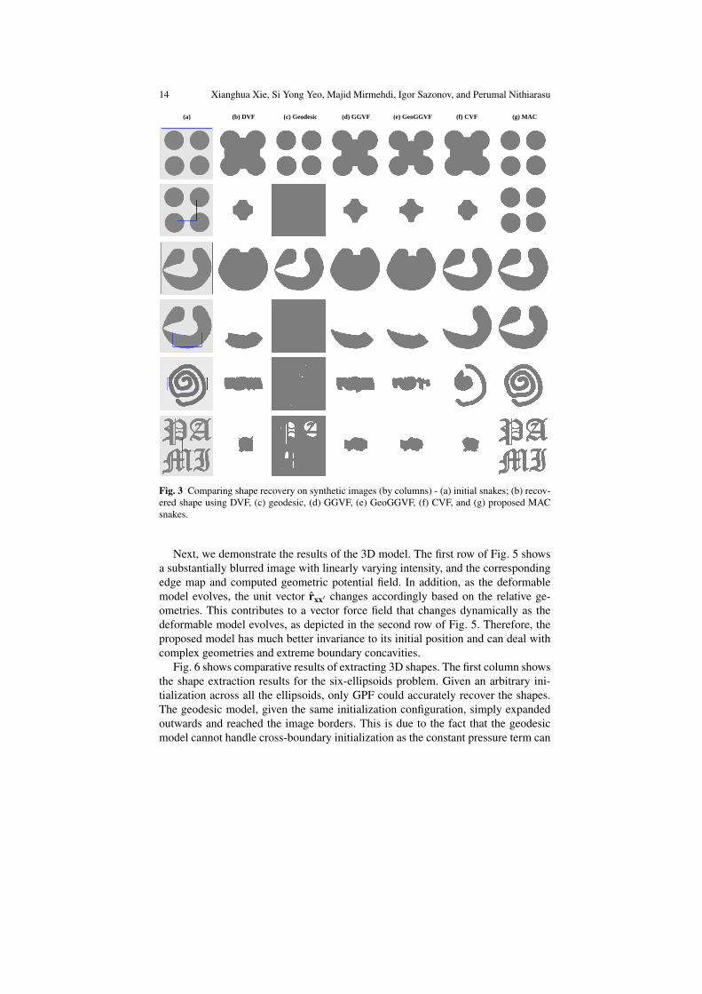
Fig. 3 shows comparative results of 2D segmentation on synthetic data. Eventhough these images have clear (ideal) boundary and the active contour models areall using level set representation, convergence issues still arise. The solution be-comes particularly challenging under certain initialization conditions. The first tworows in Fig. 3 show comparative recovered shapes for the DVF [Cohen and Co-hen(1993)], geodesic, GGVF, GeoGGVF, CVF, and MAC models in columns (b)to (g) respectively. When the initial contour was placed outside the four discs (firstrow), only the geodesic snake and MAC could accurately recover them. However,in a more arbitrary cross-boundary initialization case (second row), only MAC wassuccessful. Next, we consider the recovery of an acute concavity as shown in thethird and fourth rows in Fig. 3, again with different initialization conditions. Forthe DVF, GGVF, and GeoGGVF snakes, their stationary vector force fields exhibitstationary and saddle points, e.g. the saddle point at the entrance of the concaveshape which prevents the snake converging to the object boundaries. Again, givenan arbitrary cross-boundary initialization, the geodesic snake suffers severe prob-lems and the constriction on the left side of the concave shape causes difficultiesfor the CVF active contour. MAC was the only active contour model that couldsuccessfully recover the shape in both initializations. When dealing with complexgeometries, such as the swirl shape and the text “PAMI” shown in the last two rowsin Fig. 3, MAC was the only model that managed to fully recover the shapes. Thelatter example further illustrates MAC’s ability in dealing with multiple objects withcomplex topology.

Fig. 4 shows a brain MRI image and its comparative segmentation results. Forthe active contour models, the snake was initialized across the left and right hemi-spheres, while for the particle model a grid of charges was used. The static vectorforce based methods (DVF, GGVF, and GeoGGVF) failed to evolve through the tor-tuous structures and collapsed to nearby edges as shown in rows (a), (c), and (d).The geodesic snake, in row (b), stepped across the weak edges but also failed tolocalize the boundaries. The free charges of CPM initially reached most of the ob-ject boundaries, but later failed to stabilize at weaker edges resulting in incompleteboundary description (row (e)). The MAC contours succeeded in evolving throughthe narrow and twisted structures as shown in row (f). Multiple regions were cap-tured simultaneously.


(a) (b) DVF (c) Geodesic (d) GGVF (e) GeoGGVF (f) CVF (g) MAC

Fig. 3 Comparing shape recovery on synthetic images (by columns) - (a) initial snakes; (b) recov-ered shape using DVF, (c) geodesic, (d) GGVF, (e) GeoGGVF, (f) CVF, and (g) proposed MACsnakes.

Next, we demonstrate the results of the 3D model. The first row of Fig. 5 showsa substantially blurred image with linearly varying intensity, and the correspondingedge map and computed geometric potential field. In addition, as the deformablemodel evolves, the unit vector rxx′ changes accordingly based on the relative ge-ometries. This contributes to a vector force field that changes dynamically as thedeformable model evolves, as depicted in the second row of Fig. 5. Therefore, theproposed model has much better invariance to its initial position and can deal withcomplex geometries and extreme boundary concavities.

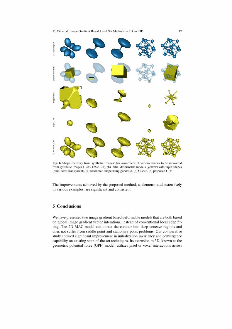
Fig. 6 shows comparative results of extracting 3D shapes. The first column showsthe shape extraction results for the six-ellipsoids problem. Given an arbitrary ini-tialization across all the ellipsoids, only GPF could accurately recover the shapes.The geodesic model, given the same initialization configuration, simply expandedoutwards and reached the image borders. This is due to the fact that the geodesicmodel cannot handle cross-boundary initialization as the constant pressure term can


(a)

DV

F(b

) ge

odes

ic(c

) G

GV

F(d

) G

eoG

GV

F(e

) C

PM

(f)

MA

C

Fig. 4 Comparative study - results by row: (a) DVF, (b) geodesic, (c) GGVF, (d) GeoGGVF, (e)CPM, (f) MAC.

only monotonically shrink or expand the contour. Although the bidirectionality ofthe GGVF model enables it to handle cross-boundary initialization, the saddle andstationary points in this example prevented GGVF from extracting the ellipsoids.The second and third columns show the geometrical object to be recovered con-sists of two flattened ellipsoids connected by a narrowing tube with a constriction inthe middle. With the deformable models initialized inside one of the ellipsoid, onlyGPF could propagate through the narrowing tube to accurately extract the shape.Also, with a more arbitrary cross-boundary initialization, GPF was the only suc-


Fig. 5 GPF: first row from left to right - input image and initial deformable model, correspondingedge map and computed geometric potential field, second row - initial and evolving deformablemodels, and the third row - associated GPF vector field.

cessful model to extract the exact shape. The fourth and fifth columns in Fig. 6compares the shape extraction results on a complex geometry with different initial-ization configurations. When the initial surface is placed inside one of the sphere ofthe molecular structure, GPF is the only model that managed to extract the geome-try successfully. These examples demonstrate the superior performance of the GPFdeformable model in resolving deep concavities and handling complex geometriesand topologies. This is mainly due to the dynamic nature of the vector force field.In addition, we show that the bidirectionality of the new force field gives GPF theflexibility to deal with arbitrary cross-initializations.

Fig. 7 shows comparative results on the segmentation of cerebral arterial struc-ture from magnetic resonance (MR) imaging. Two initial surfaces are placed insidethe object of interest for the geodesic model, and across the object boundaries forGGVF, Chan-Vese and GPF. The geodesic model cannot propagate through the nar-row tubular structures, and leaks out at weak object boundaries during the evolution.The GGVF model collapsed to the nearby object edges due to the saddle or station-ary points inside the narrow image structures. In contrast, the Chan-Vese and GPFmodels are able to propagate through the long tubular structures to extract the cere-bral arterial geometry. Further examples of the 3D method on real data are givenin Fig. 8. The examples above have shown that the GPF deformable model canefficiently segment thin and complex structures, and can handle inhomogeneity inimage intensities, noises and weak edges, which are often present in real images.


(a)

targ

et o

bjec

ts(b

) in

itial

izat

ions

(c)

geod

esic

(d)

GG

VF

(e)

prop

osed

GPF

Fig. 6 Shape recovery from synthetic images: (a) isosurfaces of various shapes to be recoveredfrom synthetic images (128×128×128), (b) initial deformable models (yellow) with input shapes(blue, semi-transparent), (c) recovered shape using geodesic, (d) GGVF, (e) proposed GPF

The improvements achieved by the proposed method, as demonstrated extensivelyin various examples, are significant and consistent.

5 Conclusions

We have presented two image gradient based deformable models that are both basedon global image gradient vector interations, instead of conventional local edge fit-ting. The 2D MAC model can attract the contour into deep concave regions anddoes not suffer from saddle point and stationary point problems. Our comparativestudy showed significant improvement in initialization invariancy and convergencecapability on existing state-of-the-art techniques. Its extension to 3D, known as thegeometric potential force (GPF) model, utilizes pixel or voxel interactions across


geod

esic

GG

VF

Cha

n-V

ese

GPF

Fig. 7 Segmentation of cerebral arterial structure using different deformable models - first row:geodesic; second row: GGVF; third row: Chan-Vese; fourth row: proposed GPF.

Fig. 8 More examples of the proposed method on real 3D medical data.


the whole image. The derived geometric potential field is thus more informative andexhibits spatial and structural characteristics of image objects which are more co-herent than image cues that are based solely on local edge or regional information.This makes the model more robust towards image noise and weak object edges. Therelativity between geometries gives the proposed deformable model its distinctivebidirectionality, which facilitates the handling of arbitrary cross-boundary initial-izations. The straightforward generalization of the proposed model to higher di-mensions allows the framework to be applied on N-dimensional images, and opensup to a wide range of potential applications.

References

[Adalsteinsson and Sethian(1998)] Adalsteinsson D, Sethian J (1998) The fast construction of ex-tension velocities in level set methods. J Comp Phy 148:2–22

[Birchfield and Tomasi(1999)] Birchfield S, Tomasi C (1999) Depth discontinuities by pixel-to-pixel stereo. IJCV 35(3):269–293

[Caselles et al(1997)Caselles, Kimmel, and Sapiro] Caselles V, Kimmel R, Sapiro G (1997)Geodesic active contour. IJCV 22(1):61–79

[Chakraborty et al(1996)Chakraborty, Staib, and Duncan] Chakraborty A, Staib H, Duncan J(1996) Deformable boundary finding in medical images by integrating gradient and regioninformation. IEEE T-MI 15(6):859–870

[Chan and Vese(2001)] Chan T, Vese L (2001) Active contours without edges. IEEE T-IP10(2):266–277

[Cohen and Cohen(1993)] Cohen L, Cohen I (1993) Finite-element methods for active contourmodels and balloons for 2-D and 3-D images. IEEE T-PAMI 15(11):1131–1147

[Cremers et al(2007)Cremers, Rousson, and Deriche] Cremers D, Rousson M, Deriche R (2007)A review of statistical approaches to level set segmentation: Integrating color, texture, motionand shape. IJCV 72(2):195–215

[Gil and Radeva(2003)] Gil D, Radeva P (2003) Curvature vector flow to assure convergent de-formable models for shape modelling. In: EMMCVPR, pp 357–372

[Haddon and Boyce(1990)] Haddon J, Boyce J (1990) Image segmentation by unifying region andboundary information. IEEE T-PAMI 12:929–948

[Hao and Li(2007)] Hao J, Li M (2007) A supervised bayesian method for cerebrovascular seg-mentation. WSEAS Trans Signal Processing 3(12):487–495

[Heidemann(2005)] Heidemann G (2005) The long-range saliency of edge- and corner-basedsaliency points. IEEE T-IP 14:1701–1706

[Jalba et al(2004)Jalba, Wilkinson, and Roerdink] Jalba A, Wilkinson M, Roerdink J (2004)CPM: A deformable model for shape recovery and segmentation based on charged particles.IEEE T-PAMI 26(10):1320–1335

[Li et al(2005)Li, Liu, and Fox] Li C, Liu J, Fox M (2005) Segmentation of edge preserving gra-dient vector flow: an approach toward automatically initializing and splitting of snakes. In:CVPR, pp 162–167

[Li et al(2007)Li, Kao, Gore, and Ding] Li C, Kao C, Gore J, Ding Z (2007) Implicit active con-tours driven by local binary fitting energy. In: CVPR, pp 1–7

[Maintz and Viergever(1998)] Maintz JB, Viergever MA (1998) A survey of medical image reg-istration. Medical Image Analysis 2(1):1–36

[Paragios and Deriche(2002)] Paragios N, Deriche R (2002) Geodesic active regions and level setmethods for supervised texture segmentation. IJCV 46(3):223–247

[Paragios et al(2004)Paragios, Mellina-Gottardo, and Ramesh] Paragios N, Mellina-Gottardo O,Ramesh V (2004) Gradient vector flow geometric active contours. IEEE T-PAMI 26(3):402–407


[Park and Chung(2002)] Park HK, Chung MJ (2002) External force of snake: virtual electric field.Electronics Letters 38(24):1500–1502

[Ruan et al(2000)Ruan, Jaggi, Xue, Fadili, and Bloyet] Ruan S, Jaggi C, Xue J, Fadili J, Bloyet D(2000) Brain tissue classification of magnetic resonance images using partial volume model-ing. IEEE T-MI 19(12):1179–1187

[Smith et al(2007)Smith, Smith, Williams, Rodriguez, and Hoying] Smith CM, Smith J, WilliamsSK, Rodriguez JJ, Hoying JB (2007) Automatic thresholding of three-dimensional microvas-cular structures from confocal microscopy images. J Microscopy 225(3):244–257

[Wu et al(2008)Wu, Ye, Ma, Sun, Xu, and Cui] Wu J, Ye F, Ma J, Sun X, Xu J, Cui Z (2008) Thesegmentation and visualization of human organs based on adaptive region growing method.In: Int. Conf. Comp. and Info. Tech., pp 439–443

[Xie(2010)] Xie X (2010) Active contouring based on gradient vector interaction and constrainedlevel set diffusion. IEEE T-IP 19(1):154–164

[Xie and Mirmehdi(2004)] Xie X, Mirmehdi M (2004) RAGS: Region-aided geometric snake.IEEE T-IP 13(5):640–652

[Xie and Mirmehdi(2008)] Xie X, Mirmehdi M (2008) MAC: Magnetostatic active contour. IEEET-PAMI 30(4):632–646

[Xu and Prince(1998)] Xu C, Prince J (1998) Snakes, shapes, & gradient vector flow. IEEE T-IP7(3):359–369

[Yang et al(2006)Yang, Mirmehdi, and Xie] Yang R, Mirmehdi M, Xie X (2006) A charged activecontour based on electrostatics. In: ACIVS, pp 173–184

[Yeo et al(2011)Yeo, Xie, Sazonov, and Nithiarasu] Yeo S, Xie X, Sazonov I, Nithiarasu P (2011)Geometrically induced force interaction for three-dimensional deformable models. IEEE T-IP20(5):1373–1387

[Zhu et al(2008)Zhu, Zhang, Zeng, and Wang] Zhu G, Zhang S, Zeng Q, Wang C (2008)Anisotropic virtual electric field for active contours. Pattern Recgnition Letters 29(11):1659–1666

Documents

Image Gradient Based Level Set Methods in 2D and 3Dcsjason/papers/xxetal.pdfImage Gradient Based Level Set Methods in 2D and 3D Xianghua Xie, Si Yong Yeo, Majid Mirmehdi, Igor Sazonov,