Embed Size (px)
Citation preview

CSE 252A, Fall 2019 Computer Vision I
Image Formation:
Geometric Camera Models
Computer Vision I
CSE 252A
Lecture 2
CSE 252A, Fall 2019 Computer Vision I
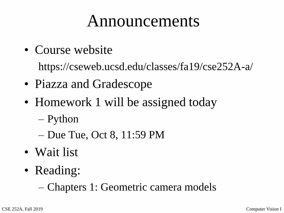
Announcements
• Course website
https://cseweb.ucsd.edu/classes/fa19/cse252A-a/
• Piazza and Gradescope
• Homework 1 will be assigned today
– Python
– Due Tue, Oct 8, 11:59 PM
• Wait list
• Reading:
– Chapters 1: Geometric camera models
CSE 252A, Fall 2019 Computer Vision I
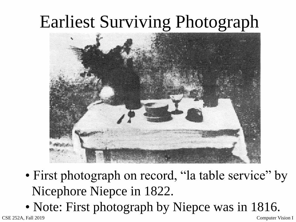
Earliest Surviving Photograph
• First photograph on record, “la table service” by
Nicephore Niepce in 1822.
• Note: First photograph by Niepce was in 1816.
CSE 252A, Fall 2019 Computer Vision I
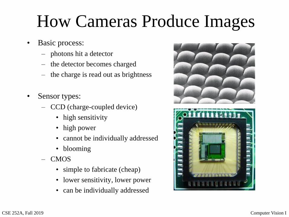
How Cameras Produce Images• Basic process:
– photons hit a detector
– the detector becomes charged
– the charge is read out as brightness
• Sensor types:
– CCD (charge-coupled device)
• high sensitivity
• high power
• cannot be individually addressed
• blooming
– CMOS
• simple to fabricate (cheap)
• lower sensitivity, lower power
• can be individually addressed
CSE 252A, Fall 2019 Computer Vision I
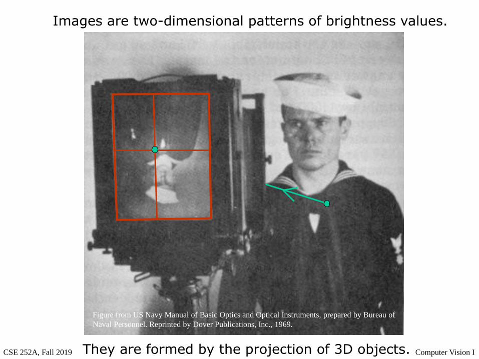
Images are two-dimensional patterns of brightness values.
They are formed by the projection of 3D objects.
Figure from US Navy Manual of Basic Optics and Optical Instruments, prepared by Bureau of
Naval Personnel. Reprinted by Dover Publications, Inc., 1969.
CSE 252A, Fall 2019 Computer Vision I
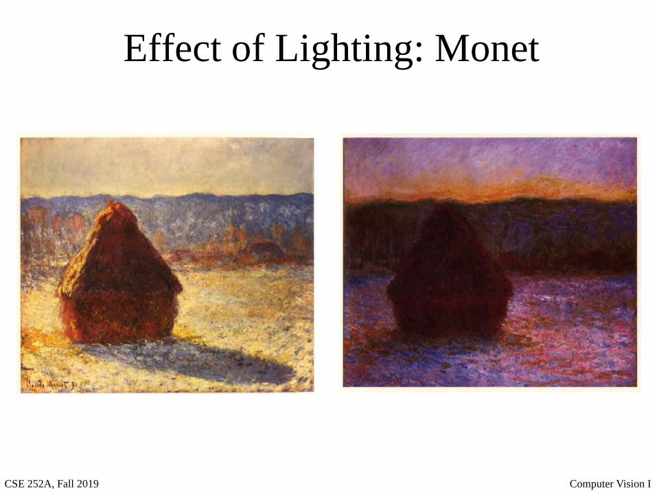
Effect of Lighting: Monet
CSE 252A, Fall 2019 Computer Vision I
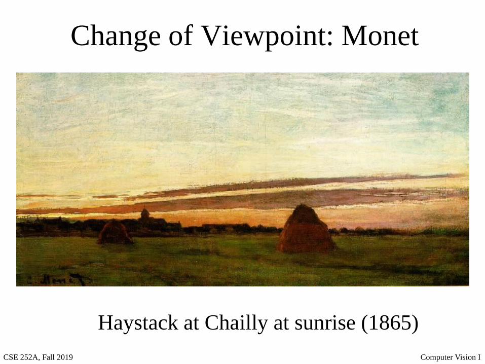
Change of Viewpoint: Monet
Haystack at Chailly at sunrise (1865)
CSE 252A, Fall 2019 Computer Vision I
Image Formation: Outline
• Geometric camera models
• Light and shading
• Color
CSE 252A, Fall 2019 Computer Vision I
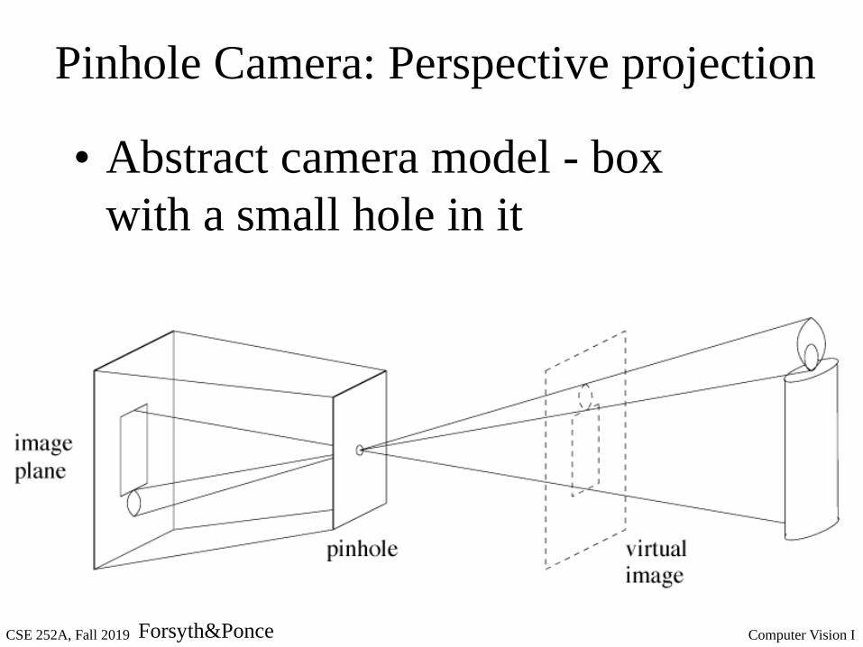
Pinhole Camera: Perspective projection
• Abstract camera model - box
with a small hole in it
Forsyth&Ponce
CSE 252A, Fall 2019 Computer Vision I
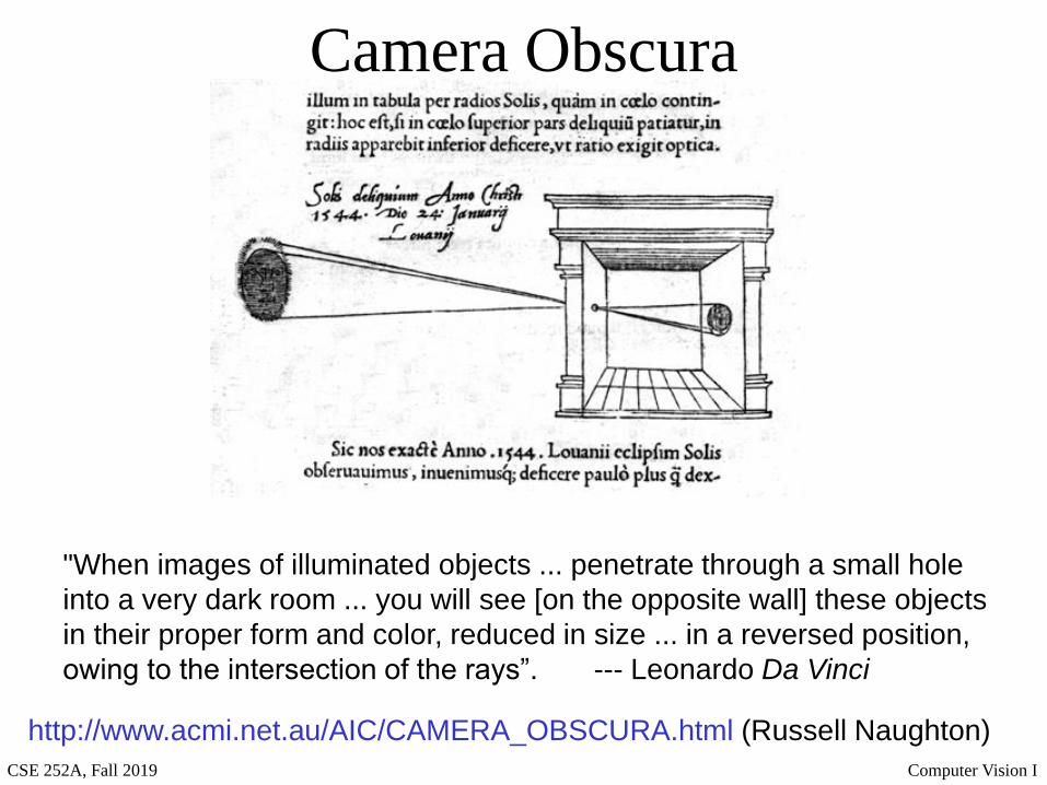
http://www.acmi.net.au/AIC/CAMERA_OBSCURA.html (Russell Naughton)
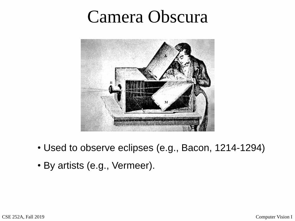
Camera Obscura
"When images of illuminated objects ... penetrate through a small hole
into a very dark room ... you will see [on the opposite wall] these objects
in their proper form and color, reduced in size ... in a reversed position,
owing to the intersection of the rays”. --- Leonardo Da Vinci
CSE 252A, Fall 2019 Computer Vision I
• Used to observe eclipses (e.g., Bacon, 1214-1294)
• By artists (e.g., Vermeer).
Camera Obscura
CSE 252A, Fall 2019 Computer Vision I
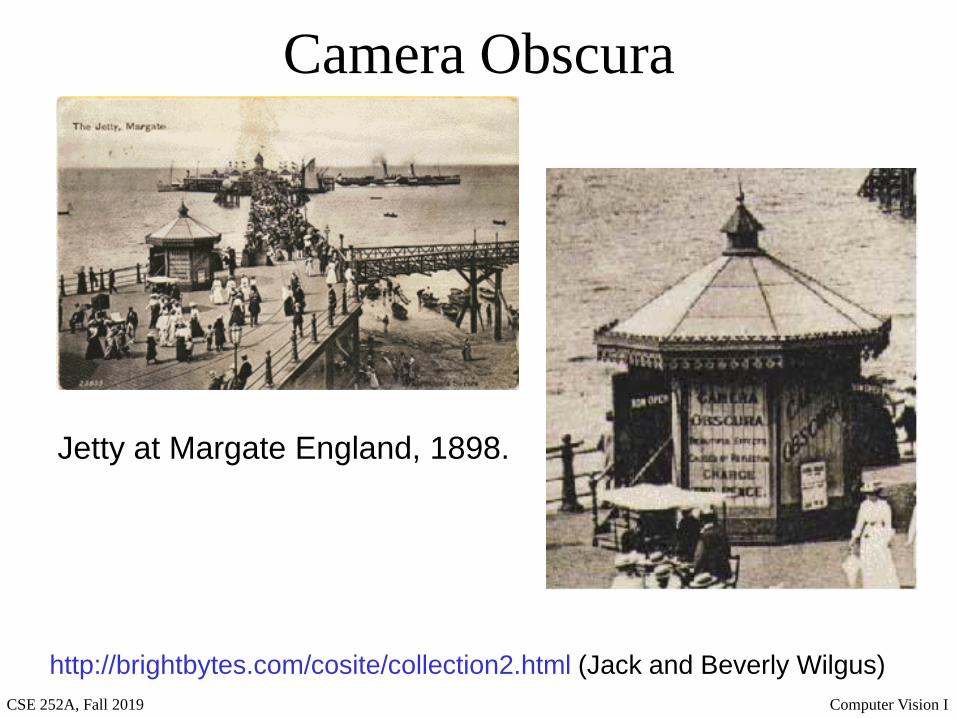
http://brightbytes.com/cosite/collection2.html (Jack and Beverly Wilgus)
Jetty at Margate England, 1898.
Camera Obscura
CSE 252A, Fall 2019 Computer Vision I(Forsyth & Ponce)
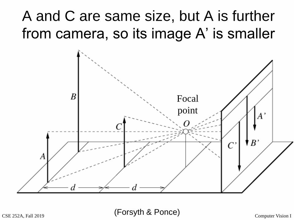
A and C are same size, but A is further
from camera, so its image A’ is smaller
Focal
point
CSE 252A, Fall 2019 Computer Vision I
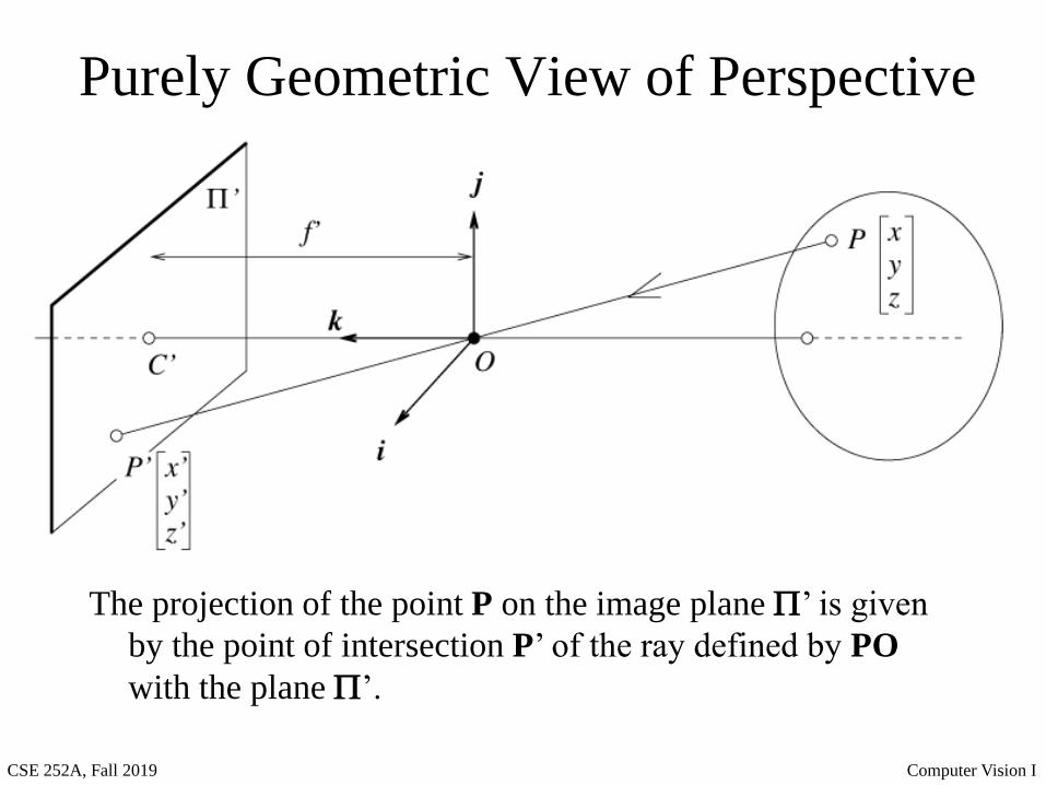
Purely Geometric View of Perspective
The projection of the point P on the image plane ’ is given
by the point of intersection P’ of the ray defined by PO
with the plane ’.
CSE 252A, Fall 2019 Computer Vision I
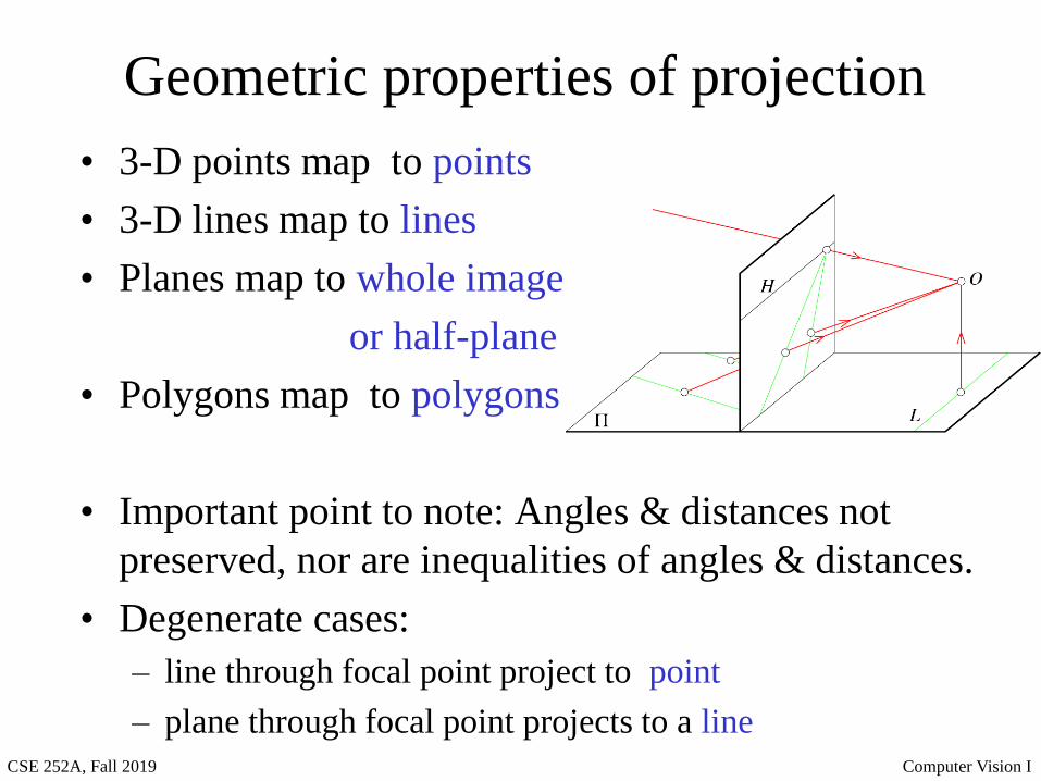
Geometric properties of projection
• 3-D points map to points
• 3-D lines map to lines
• Planes map to whole image
or half-plane
• Polygons map to polygons
• Important point to note: Angles & distances not
preserved, nor are inequalities of angles & distances.
• Degenerate cases:
– line through focal point project to point
– plane through focal point projects to a line
CSE 252A, Fall 2019 Computer Vision I
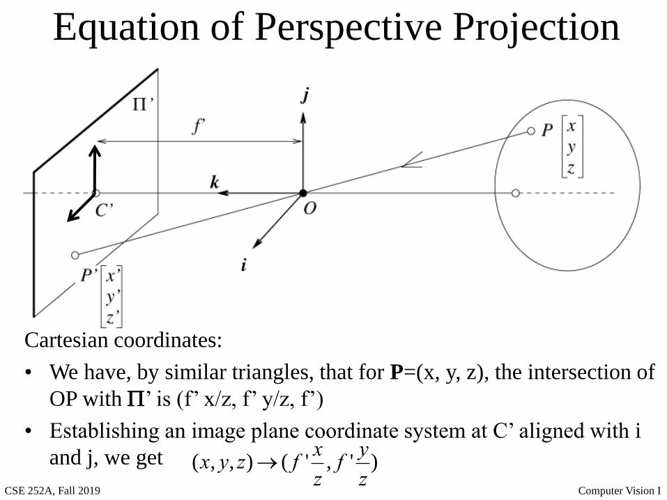
Equation of Perspective Projection
Cartesian coordinates:
• We have, by similar triangles, that for P=(x, y, z), the intersection of
OP with ’ is (f’ x/z, f’ y/z, f’)
• Establishing an image plane coordinate system at C’ aligned with i
and j, we get (x, y, z)® ( f 'x
z, f 'y
z)
CSE 252A, Fall 2019 Computer Vision I
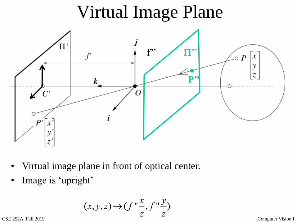
Virtual Image Plane
• Virtual image plane in front of optical center.
• Image is ‘upright’
(x, y, z)® ( f ''x
z, f ''
y
z)
’’f’’
P’’
CSE 252A, Fall 2019 Computer Vision I
A Digression
Projective Geometry
and
Homogenous Coordinates
CSE 252A, Fall 2019 Computer Vision I
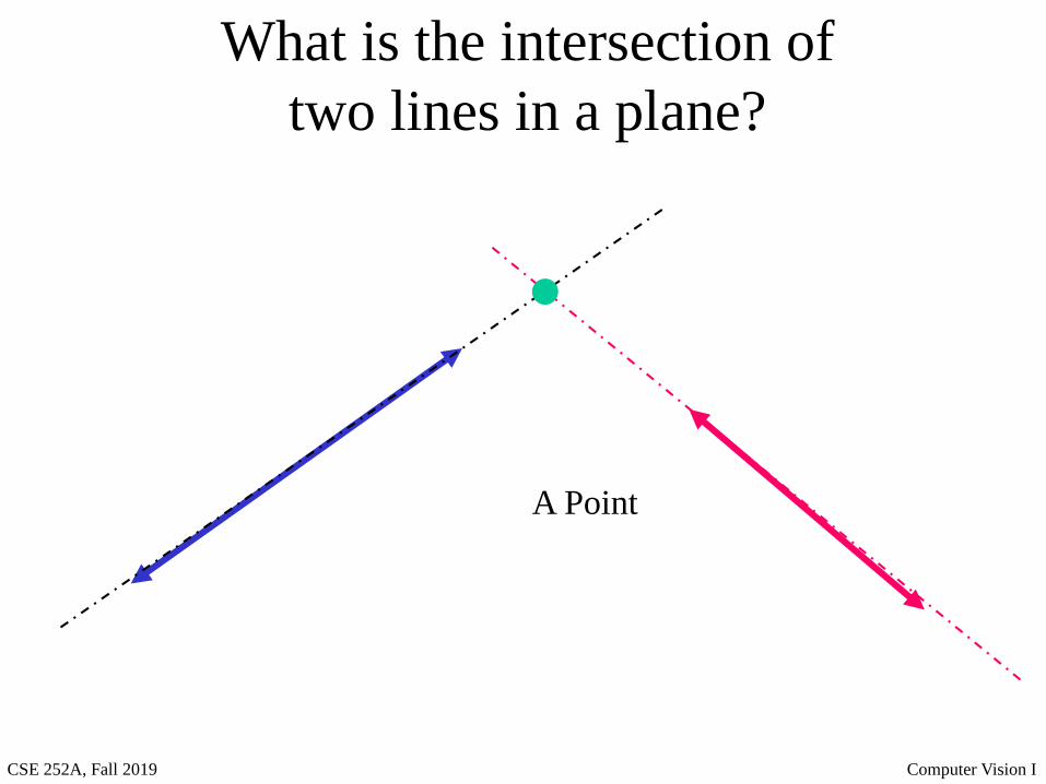
What is the intersection of
two lines in a plane?
A Point
CSE 252A, Fall 2019 Computer Vision I
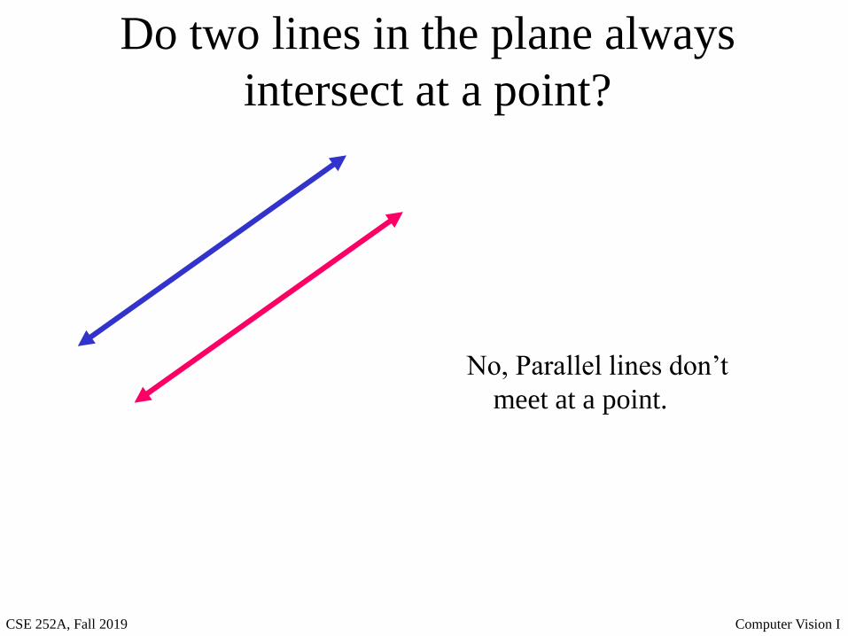
Do two lines in the plane always
intersect at a point?
No, Parallel lines don’t
meet at a point.
CSE 252A, Fall 2019 Computer Vision I
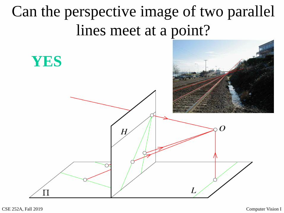
Can the perspective image of two parallel
lines meet at a point?
YES
CSE 252A, Fall 2019 Computer Vision I
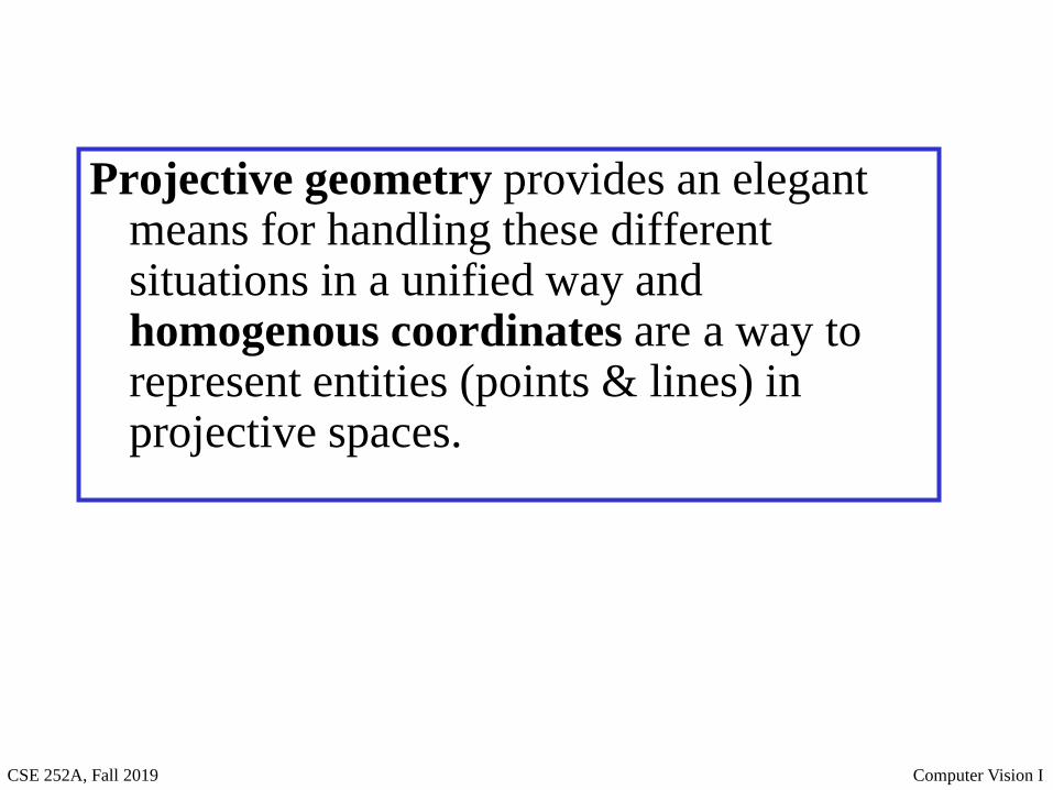
Projective geometry provides an elegant means for handling these different situations in a unified way and homogenous coordinates are a way to represent entities (points & lines) in projective spaces.
CSE 252A, Fall 2019 Computer Vision I
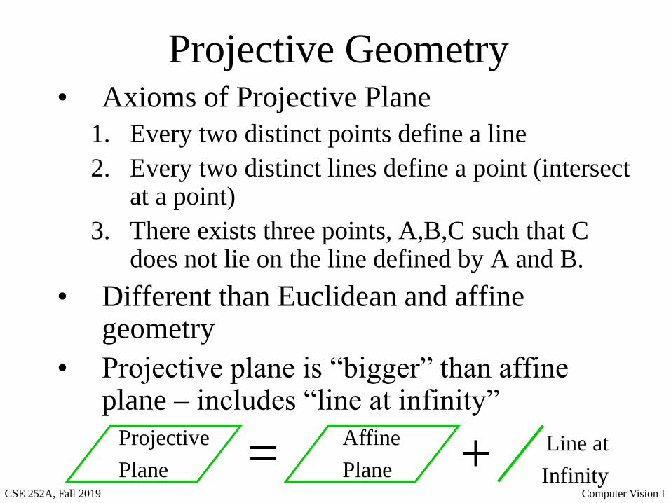
Projective Geometry• Axioms of Projective Plane
1. Every two distinct points define a line
2. Every two distinct lines define a point (intersect at a point)
3. There exists three points, A,B,C such that C does not lie on the line defined by A and B.
• Different than Euclidean and affine geometry
• Projective plane is “bigger” than affine plane – includes “line at infinity”
Projective
Plane
Affine
Plane= + Line at
Infinity
CSE 252A, Fall 2019 Computer Vision I
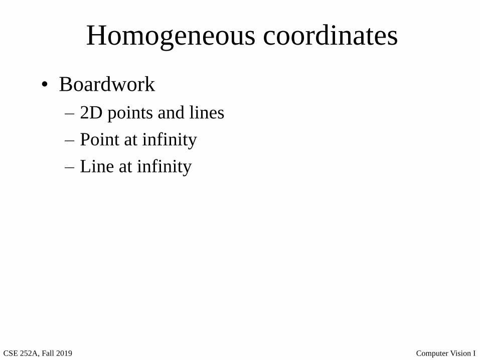
Homogeneous coordinates
• Boardwork
– 2D points and lines
– Point at infinity
– Line at infinity
CSE 252A, Fall 2019 Computer Vision I
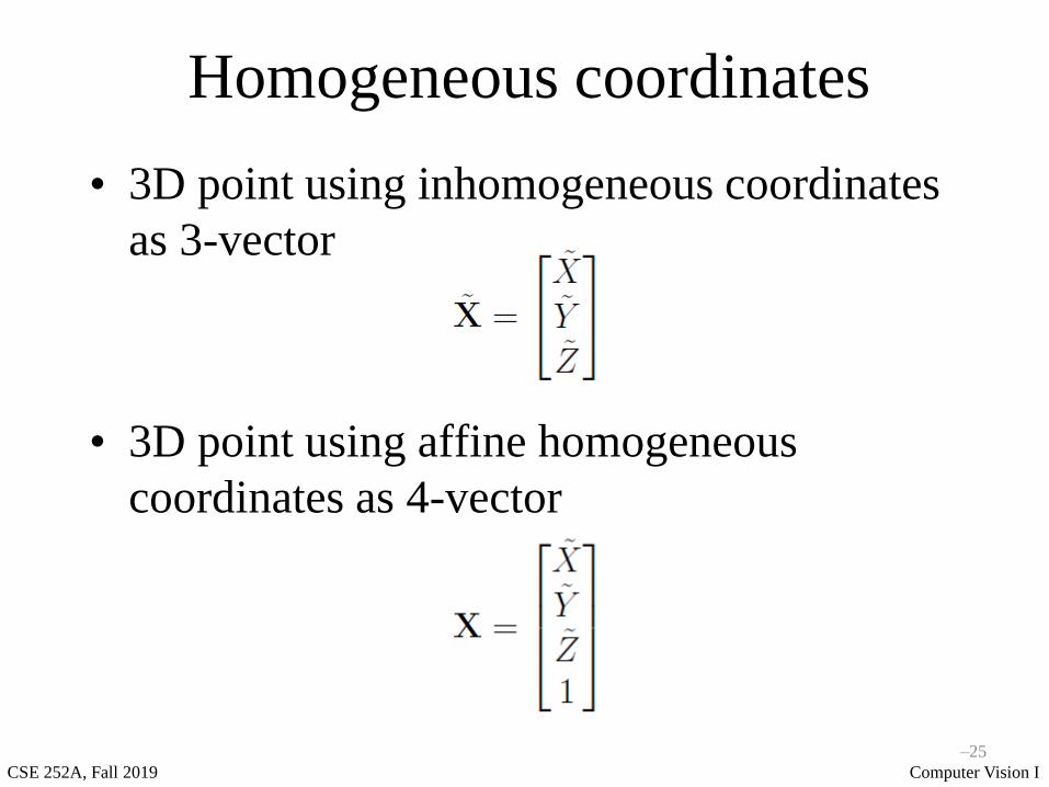
Homogeneous coordinates
• 3D point using inhomogeneous coordinates
as 3-vector
• 3D point using affine homogeneous
coordinates as 4-vector
–25
CSE 252A, Fall 2019 Computer Vision I
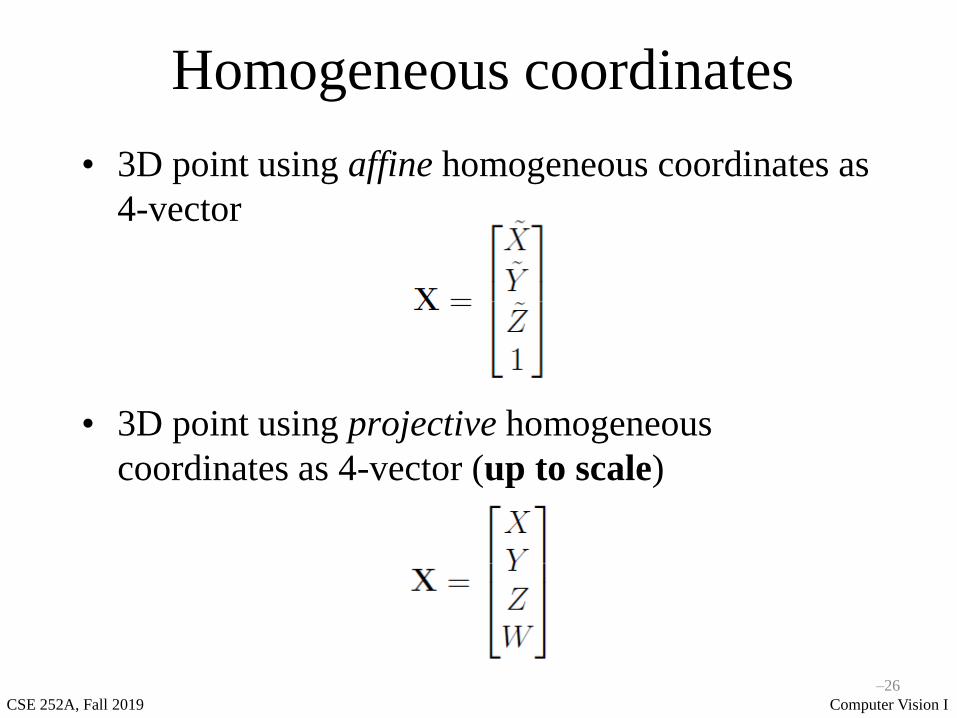
Homogeneous coordinates
• 3D point using affine homogeneous coordinates as
4-vector
• 3D point using projective homogeneous
coordinates as 4-vector (up to scale)
–26
CSE 252A, Fall 2019 Computer Vision I
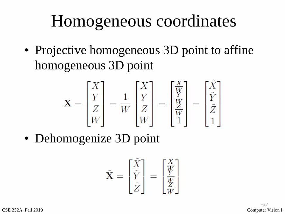
Homogeneous coordinates
• Projective homogeneous 3D point to affine
homogeneous 3D point
• Dehomogenize 3D point
–27
CSE 252A, Fall 2019 Computer Vision I
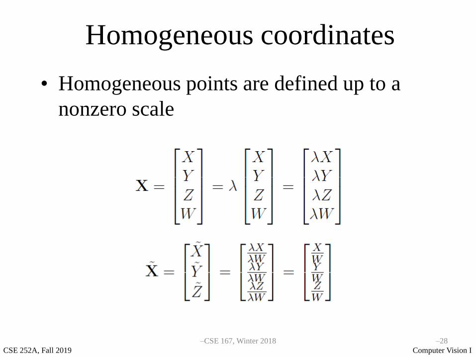
Homogeneous coordinates
• Homogeneous points are defined up to a
nonzero scale
–CSE 167, Winter 2018 –28
CSE 252A, Fall 2019 Computer Vision I
Homogeneous coordinates
• When W = 0, then it is a point at infinity
• Affine homogeneous coordinates are
projective homogeneous coordinates where
W = 1
• When not differentiating between affine
homogeneous coordinates and projective
homogeneous coordinates, simply call them
homogeneous coordinates
–CSE 167, Winter 2018 –29

CSE 252A, Fall 2019 Computer Vision I
End of the Digression
CSE 252A, Fall 2019 Computer Vision I
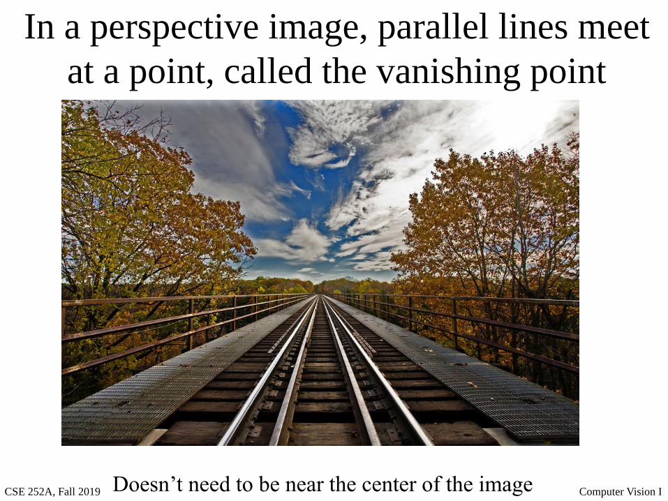
In a perspective image, parallel lines meet
at a point, called the vanishing point
Doesn’t need to be near the center of the image
CSE 252A, Fall 2019 Computer Vision I
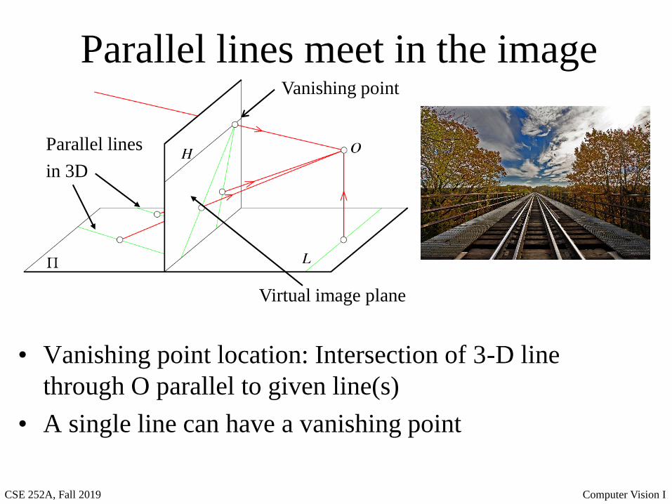
Parallel lines meet in the image
Virtual image plane
• Vanishing point location: Intersection of 3-D line
through O parallel to given line(s)
• A single line can have a vanishing point
Vanishing point
Parallel lines
in 3D
CSE 252A, Fall 2019 Computer Vision I
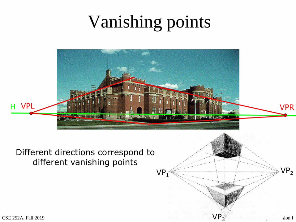
Vanishing points
VPL VPRH
VP1VP2
VP3
Different directions correspond to different vanishing points
CSE 252A, Fall 2019 Computer Vision I
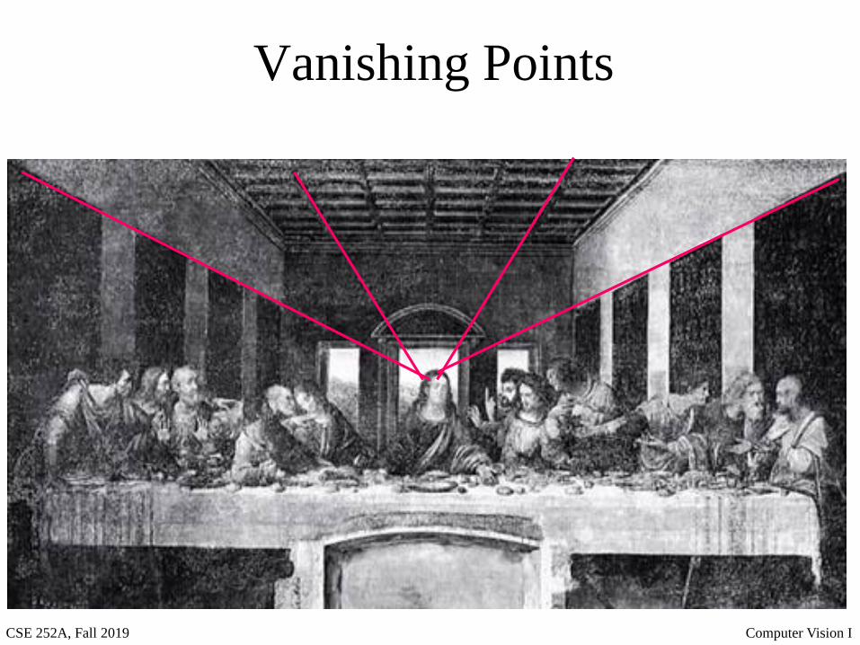
Vanishing Points
CSE 252A, Fall 2019 Computer Vision I
Vanishing Point
• In the projective plane, parallel lines meet
at a point at infinity.
• The 2D vanishing point in the image is the
perspective projection of this 3D point at
infinity
CSE 252A, Fall 2019 Computer Vision I
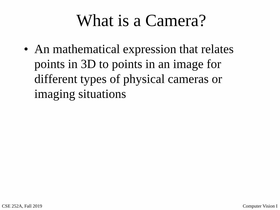
What is a Camera?
• An mathematical expression that relates
points in 3D to points in an image for
different types of physical cameras or
imaging situations
CSE 252A, Fall 2019 Computer Vision I
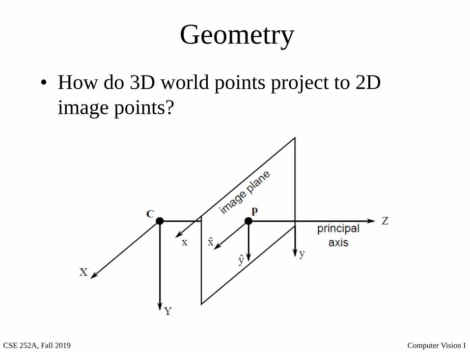
Geometry
• How do 3D world points project to 2D
image points?
CSE 252A, Fall 2019 Computer Vision I
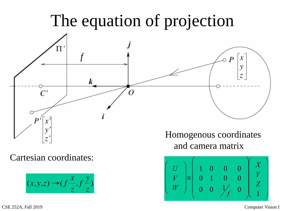
The equation of projection
Cartesian coordinates:U
V
W
æ
è
ççç
ö
ø
÷÷÷=
1 0 0 0
0 1 0 0
0 0 1f
0
æ
è
çççç
ö
ø
÷÷÷÷
X
Y
Z
1
æ
è
çççç
ö
ø
÷÷÷÷
Homogenous coordinates
and camera matrix
f
CSE 252A, Fall 2019 Computer Vision I
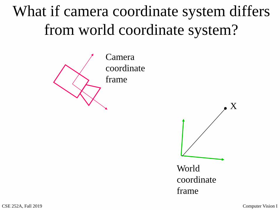
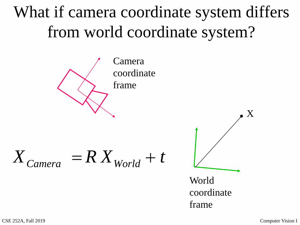
What if camera coordinate system differs
from world coordinate system?
Camera
coordinate
frame
X
World
coordinate
frame
CSE 252A, Fall 2019 Computer Vision I
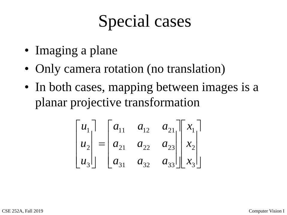
Special cases
• Imaging a plane
• Only camera rotation (no translation)
• In both cases, mapping between images is a
planar projective transformation
=
3
2
1
333231
232221
211211
3
2
1
x
x
x
aaa
aaa
aaa
u
u
u
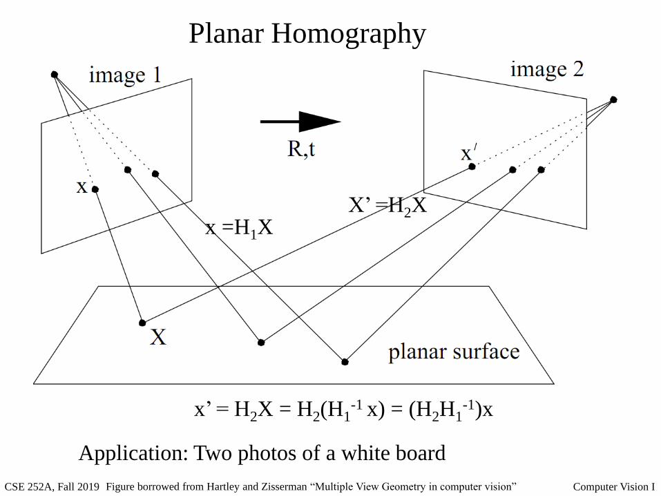
CSE 252A, Fall 2019 Computer Vision IFigure borrowed from Hartley and Zisserman “Multiple View Geometry in computer vision”
Planar Homography
x =H1XX’ =H2X
x’ = H2X = H2(H1-1 x) = (H2H1
-1)x
Application: Two photos of a white board
CSE 252A, Fall 2019 Computer Vision IFigure borrowed from Hartley and Zisserman “Multiple View Geometry in computer vision”
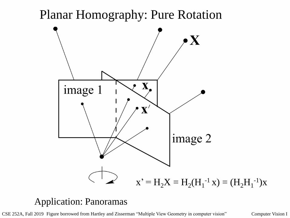
Planar Homography: Pure Rotation
x’ = H2X = H2(H1-1 x) = (H2H1
-1)x
Application: Panoramas
CSE 252A, Fall 2019 Computer Vision I
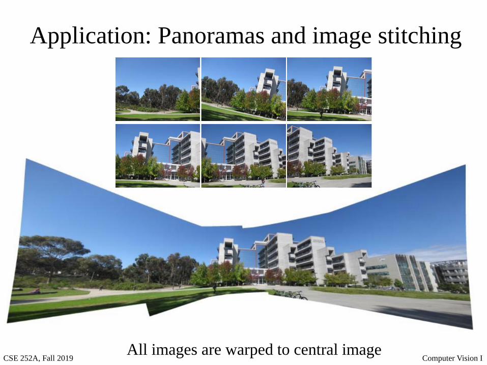
Application: Panoramas and image stitching
All images are warped to central image
CSE 252A, Fall 2019 Computer Vision I
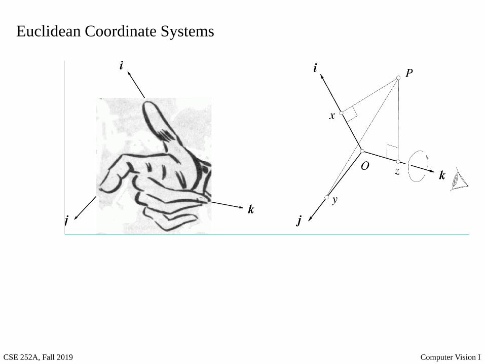
Euclidean Coordinate Systems
CSE 252A, Fall 2019 Computer Vision I
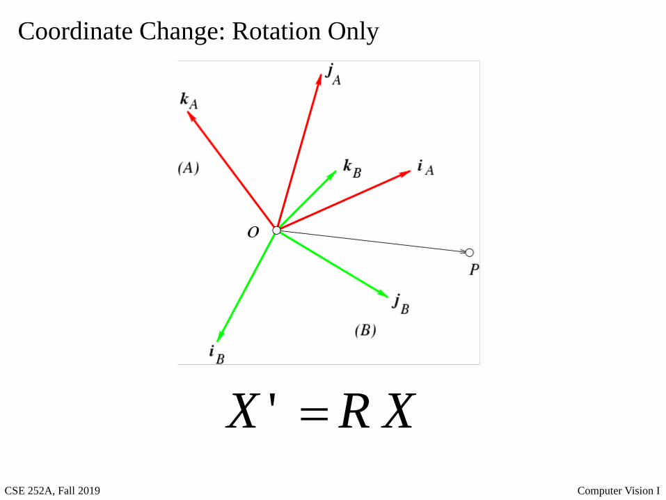
Coordinate Change: Rotation Only
XRX ='
CSE 252A, Fall 2019 Computer Vision I
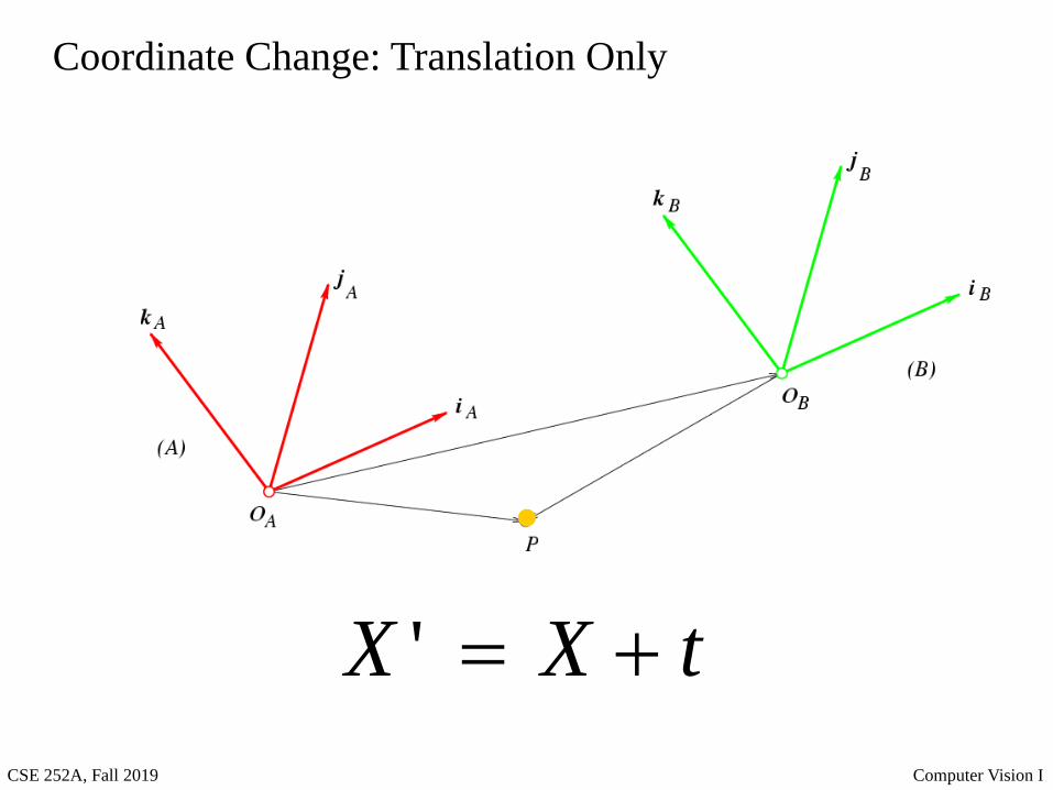
Coordinate Change: Translation Only
tXX +='
CSE 252A, Fall 2019 Computer Vision I
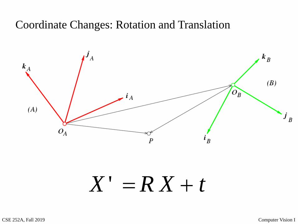
Coordinate Changes: Rotation and Translation
tXRX +='
CSE 252A, Fall 2019 Computer Vision I
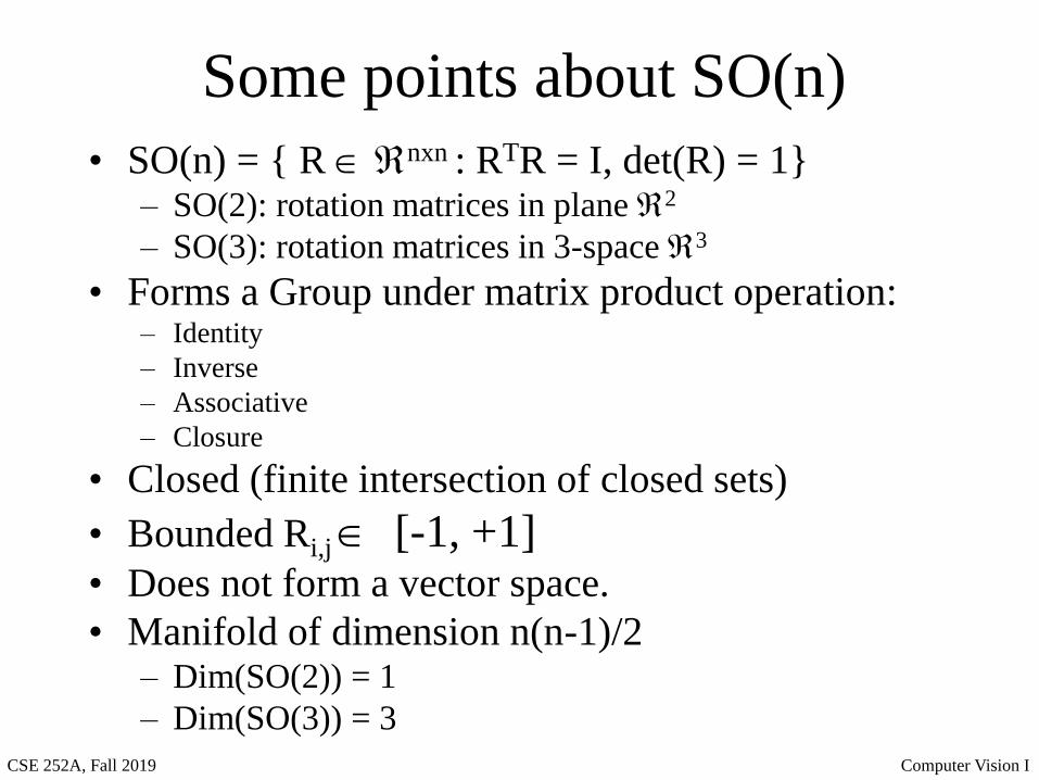
Some points about SO(n)
• SO(n) = { R nxn : RTR = I, det(R) = 1}– SO(2): rotation matrices in plane 2
– SO(3): rotation matrices in 3-space 3
• Forms a Group under matrix product operation:– Identity
– Inverse
– Associative
– Closure
• Closed (finite intersection of closed sets)
• Bounded Ri,j [-1, +1]• Does not form a vector space.
• Manifold of dimension n(n-1)/2– Dim(SO(2)) = 1
– Dim(SO(3)) = 3
CSE 252A, Fall 2019 Computer Vision I
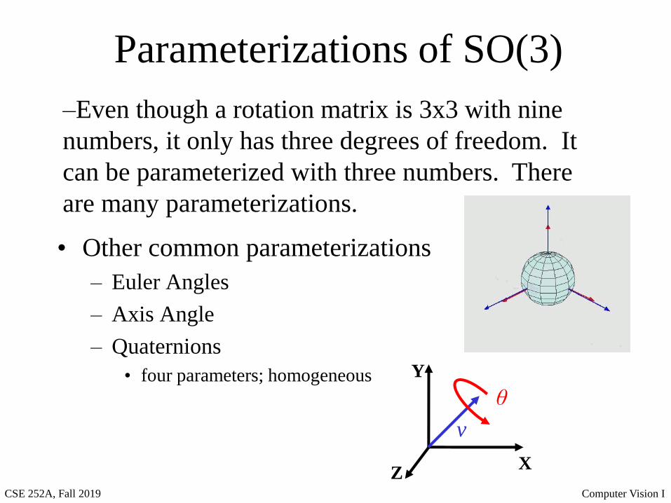
Parameterizations of SO(3)
• Other common parameterizations
– Euler Angles
– Axis Angle
– Quaternions
• four parameters; homogeneous
–Even though a rotation matrix is 3x3 with nine
numbers, it only has three degrees of freedom. It
can be parameterized with three numbers. There
are many parameterizations.
X
Y
Z
θ
v
CSE 252A, Fall 2019 Computer Vision I
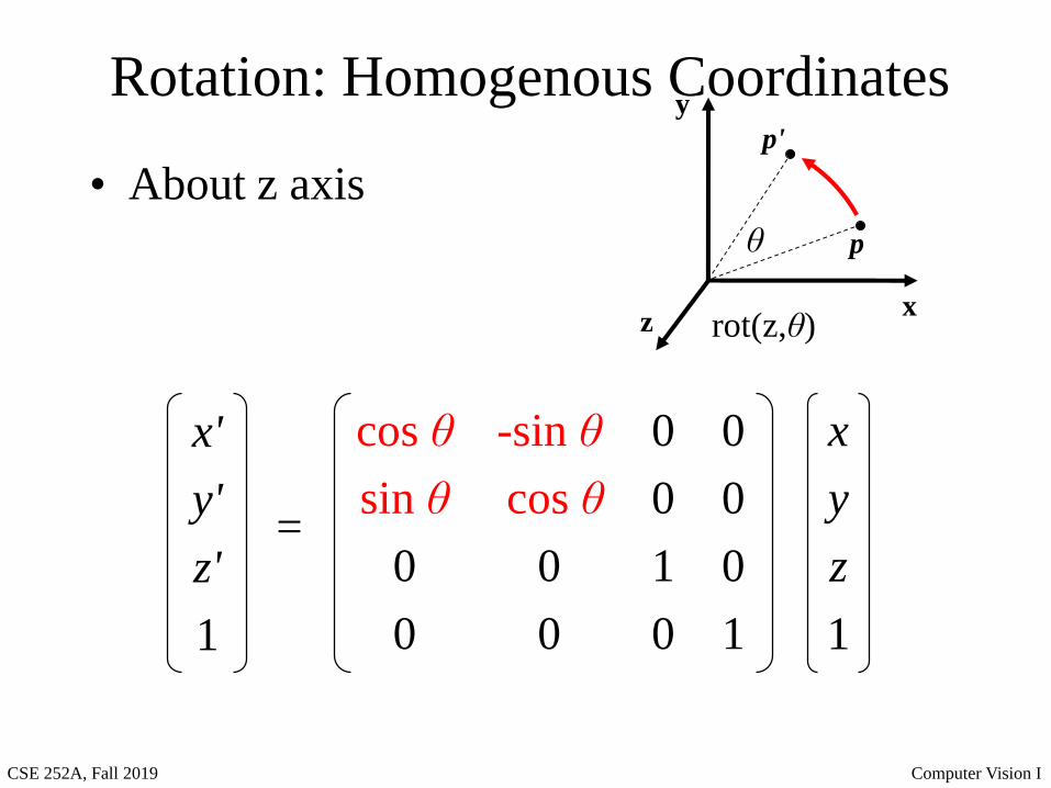
Rotation: Homogenous Coordinates
• About z axis
x'
y'
z'
1
=
x
y
z
1
cos θ
sin θ
0
0
-sin θ
cos θ
0
0
0
0
1
0
0
0
0
1
rot(z,θ)x
y
z
p
p'
θ
CSE 252A, Fall 2019 Computer Vision I
Rotation
• About
x axis:
• About
y axis:
x'
y'
z'
1
=
x
y
z
1
0
cos θ
sin θ
0
0
-sin θ
cos θ
0
1
0
0
0
0
0
0
1
x'
y'
z'
1
=
x
y
z
1
cos θ
0
-sin θ
0
sin θ
0
cos θ
0
0
1
0
0
0
0
0
1
CSE 252A, Fall 2019 Computer Vision I
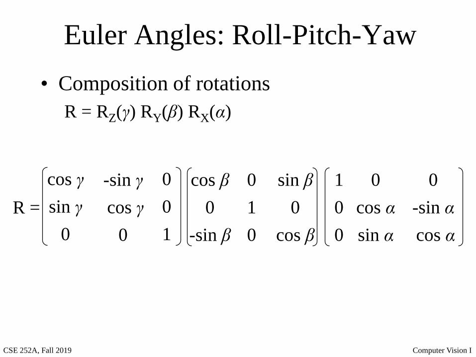
Euler Angles: Roll-Pitch-Yaw
• Composition of rotations
R = RZ(γ) RY(β) RX(α)
cos γ
sin γ
0
-sin γ
cos γ
0
0
0
1
sin β
0
cos β
cos β
0
-sin β
0
1
0
0
-sin α
cos α
0
cos α
sin α
1
0
0
R =
CSE 252A, Fall 2019 Computer Vision I
What if camera coordinate system differs
from world coordinate system?
Camera
coordinate
frame
X
World
coordinate
frame
tXRX WorldCamera +=
CSE 252A, Fall 2019 Computer Vision I
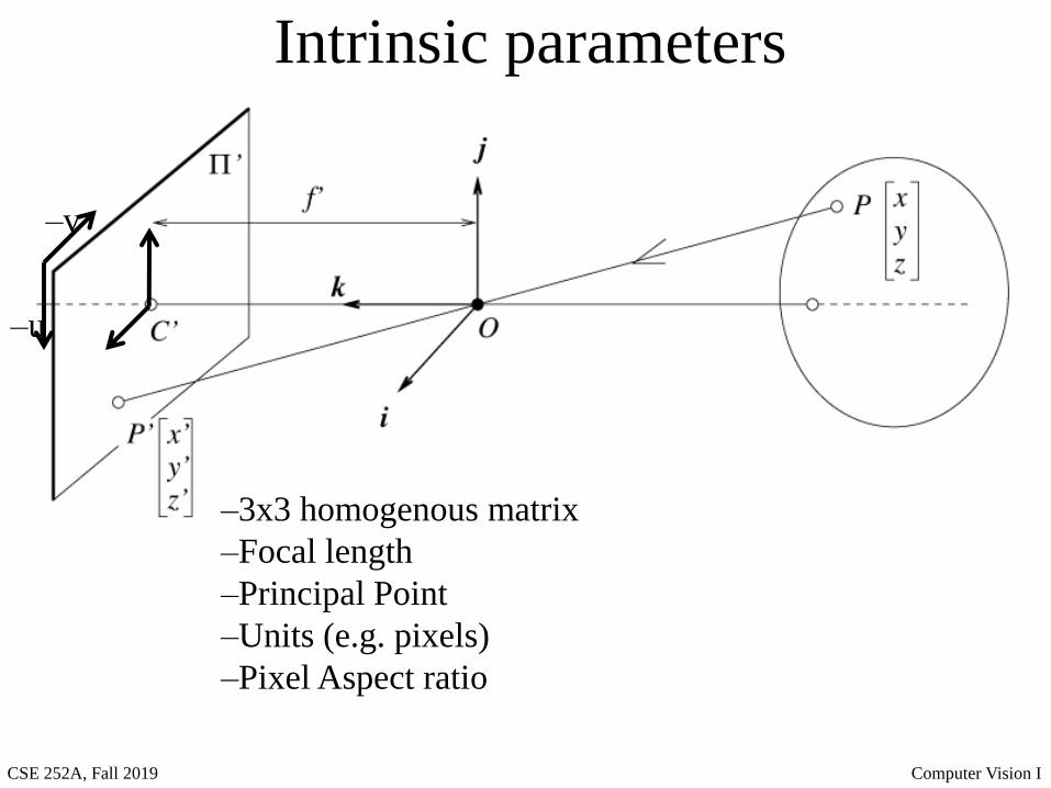
Intrinsic parameters
–u
–v
–3x3 homogenous matrix
–Focal length
–Principal Point
–Units (e.g. pixels)
–Pixel Aspect ratio
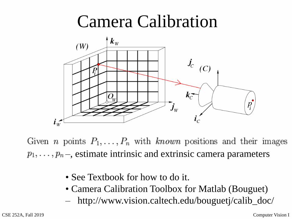
CSE 252A, Fall 2019 Computer Vision I
–, estimate intrinsic and extrinsic camera parameters
• See Textbook for how to do it.
• Camera Calibration Toolbox for Matlab (Bouguet)
– http://www.vision.caltech.edu/bouguetj/calib_doc/
Camera Calibration
CSE 252A, Fall 2019 Computer Vision I
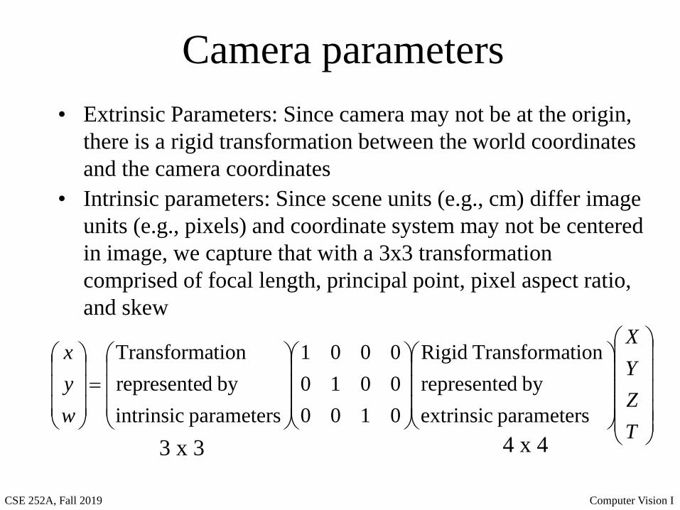
Camera parameters
• Extrinsic Parameters: Since camera may not be at the origin,
there is a rigid transformation between the world coordinates
and the camera coordinates
• Intrinsic parameters: Since scene units (e.g., cm) differ image
units (e.g., pixels) and coordinate system may not be centered
in image, we capture that with a 3x3 transformation
comprised of focal length, principal point, pixel aspect ratio,
and skew
=
T
Z
Y
X
w
y
x
parameters extrinsic
by drepresente
tionTransforma Rigid
0100
0010
0001
parameters intrinsic
by drepresente
tionTransforma
3 x 3 4 x 4
CSE 252A, Fall 2019 Computer Vision I
Camera ModelsPerspective
Projection
Scaled
Orthographic
Projection
Affine
Camera
Model
Orthographic
Projection
Parallel Projection
Camera Models
CSE 252A, Fall 2019 Computer Vision I
For all cameras?
CSE 252A, Fall 2019 Computer Vision I
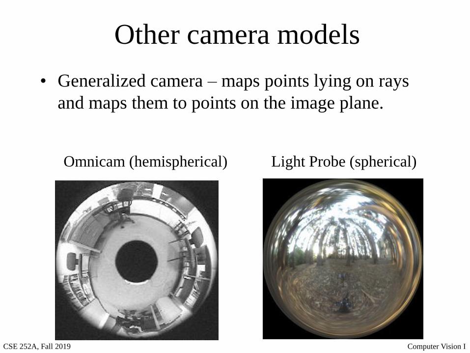
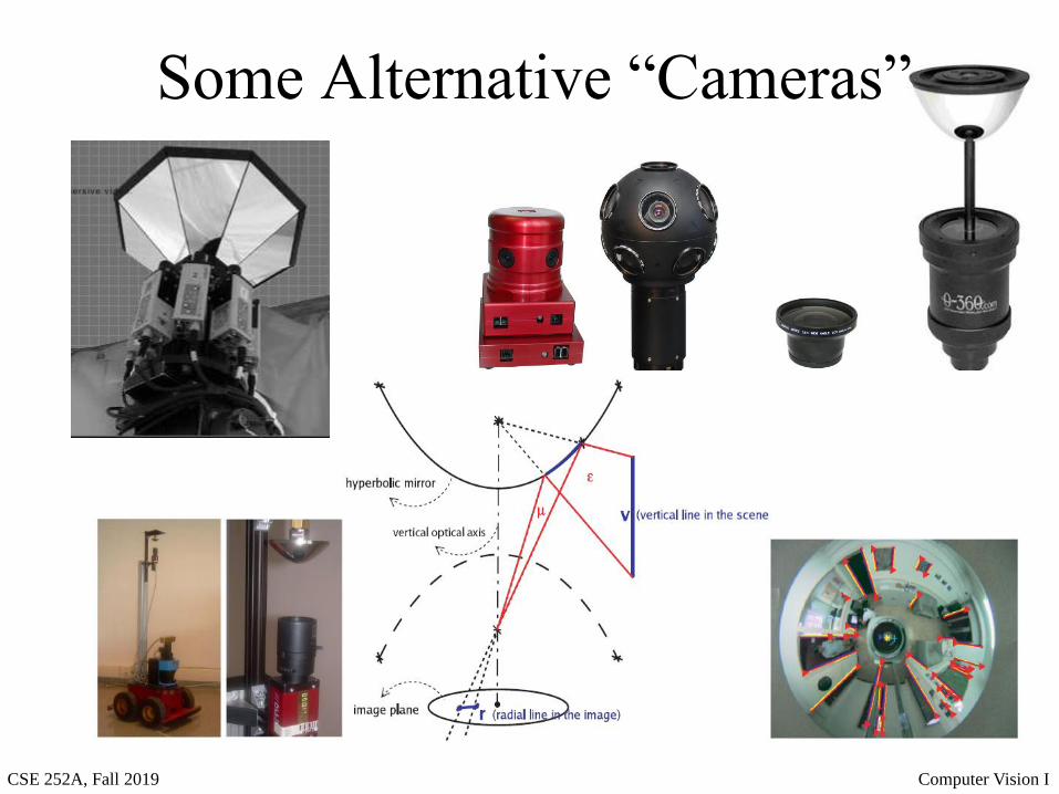
Other camera models
• Generalized camera – maps points lying on rays
and maps them to points on the image plane.
Omnicam (hemispherical) Light Probe (spherical)
CSE 252A, Fall 2019 Computer Vision I
Some Alternative “Cameras”
CSE 252A, Fall 2019 Computer Vision I
Lenses
CSE 252A, Fall 2019 Computer Vision I
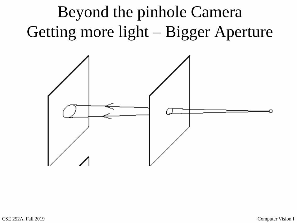
Beyond the pinhole Camera
Getting more light – Bigger Aperture
CSE 252A, Fall 2019 Computer Vision I
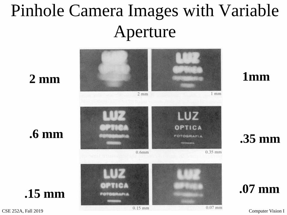
Pinhole Camera Images with Variable
Aperture
1mm
.35 mm
.07 mm
.6 mm
2 mm
.15 mm
CSE 252A, Fall 2019 Computer Vision I
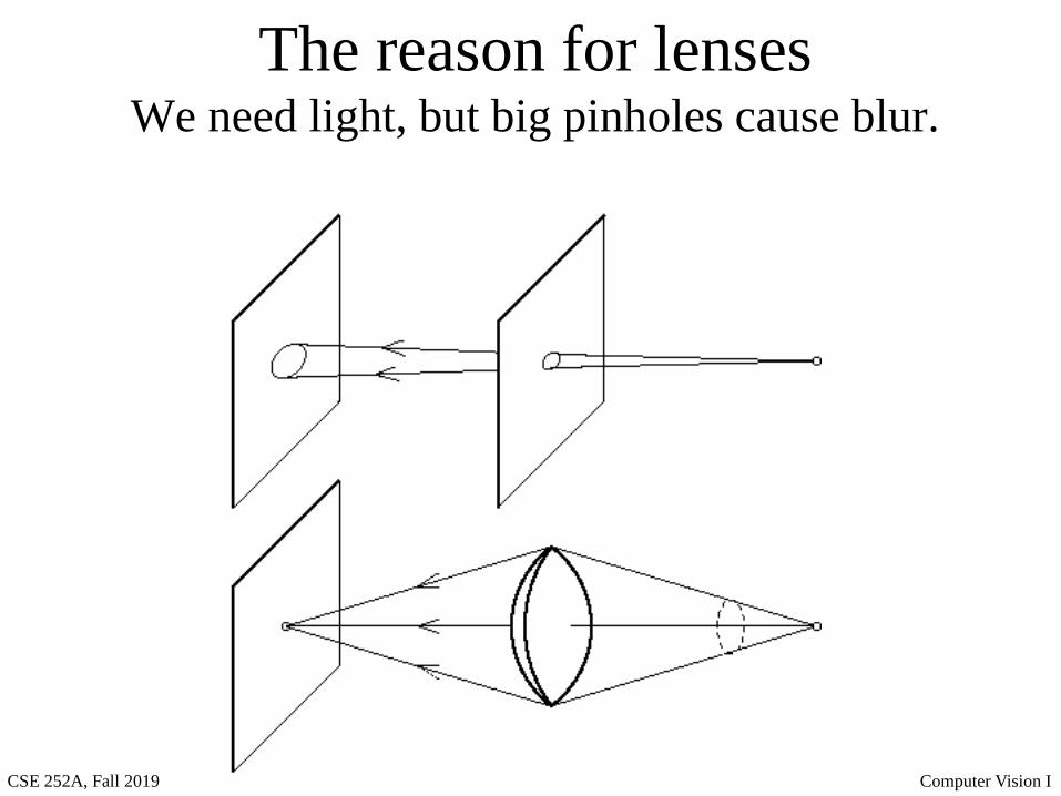
The reason for lensesWe need light, but big pinholes cause blur.
CSE 252A, Fall 2019 Computer Vision I
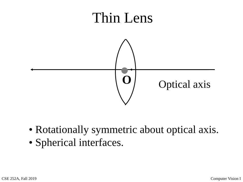
Thin Lens
O
• Rotationally symmetric about optical axis.
• Spherical interfaces.
Optical axis
CSE 252A, Fall 2019 Computer Vision I
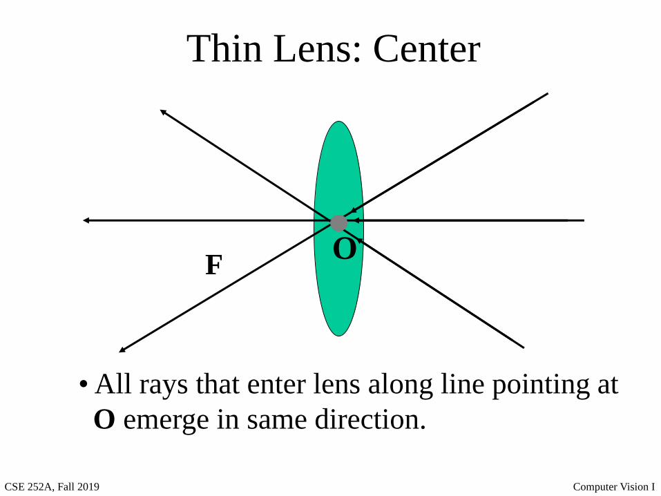
Thin Lens: Center
O
• All rays that enter lens along line pointing at
O emerge in same direction.
F
CSE 252A, Fall 2019 Computer Vision I
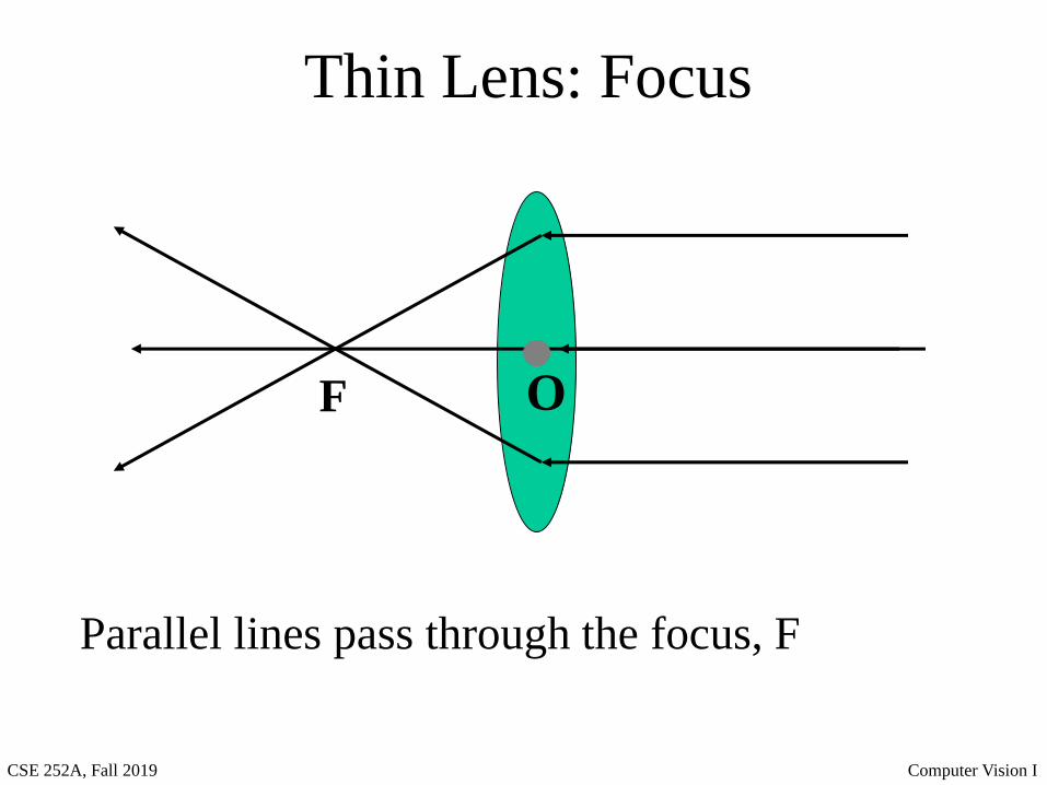
Thin Lens: Focus
O
Parallel lines pass through the focus, F
F
CSE 252A, Fall 2019 Computer Vision I
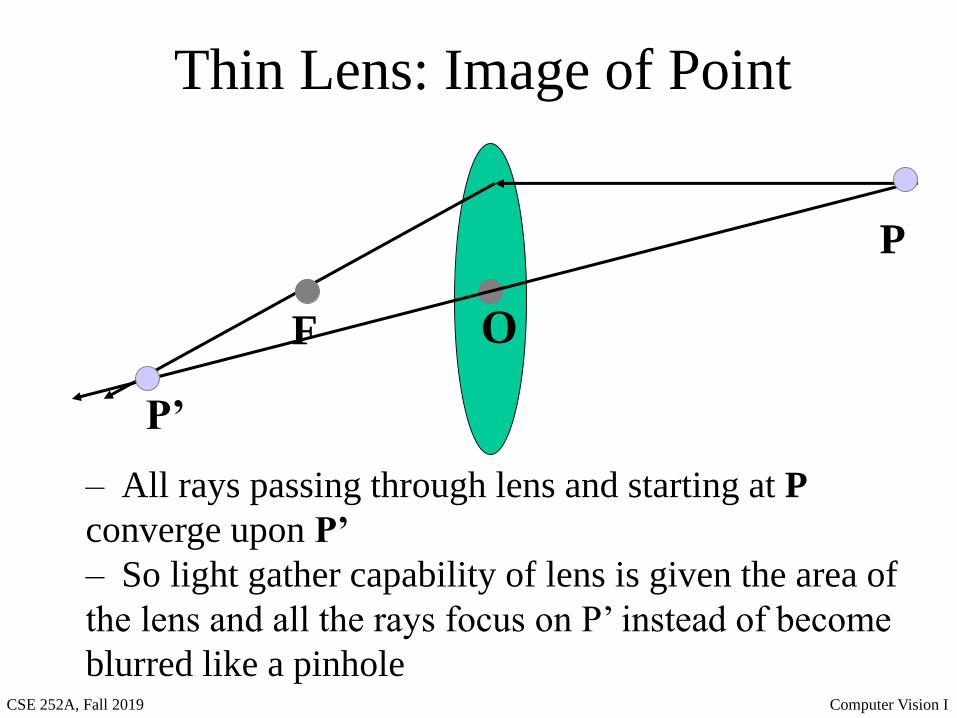
Thin Lens: Image of Point
O
– All rays passing through lens and starting at P
converge upon P’
– So light gather capability of lens is given the area of
the lens and all the rays focus on P’ instead of become
blurred like a pinhole
F
P
P’
CSE 252A, Fall 2019 Computer Vision I
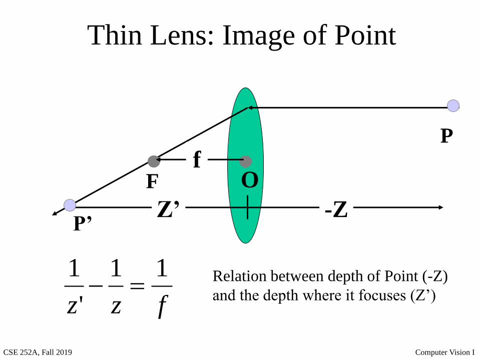
Thin Lens: Image of Point
OF
P
P’Z’
f
-Z
fzz
11
'
1=− Relation between depth of Point (-Z)
and the depth where it focuses (Z’)
CSE 252A, Fall 2019 Computer Vision I
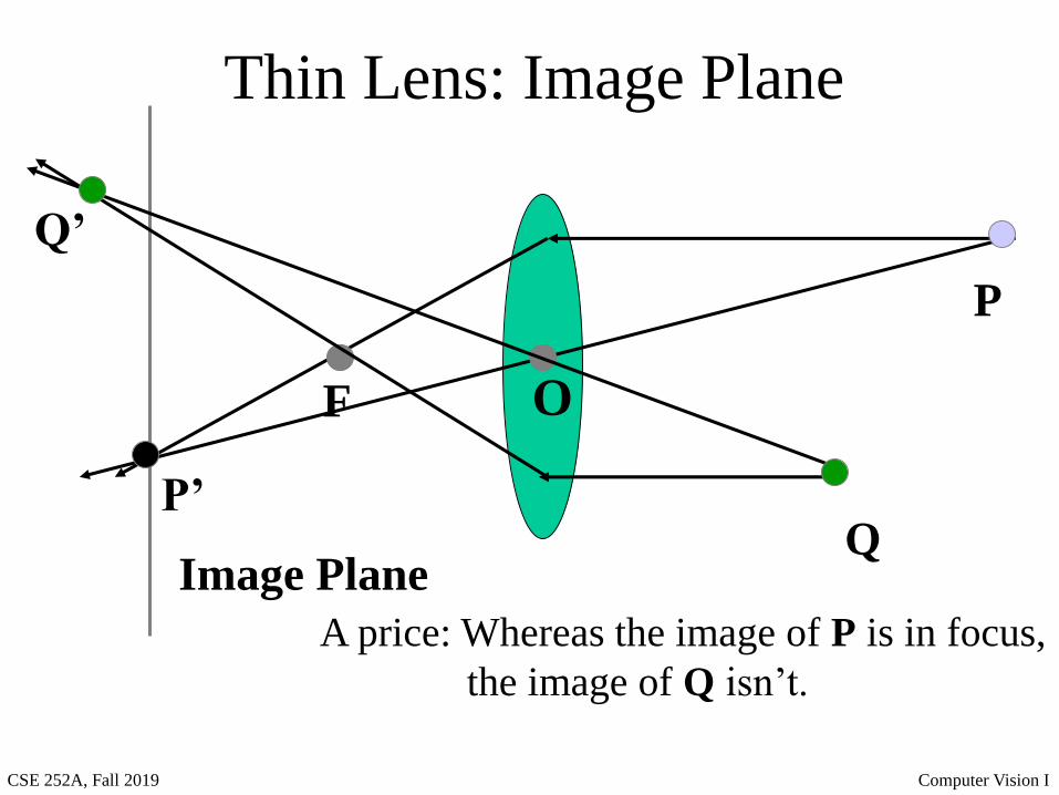
Thin Lens: Image Plane
OF
P
P’
Image Plane
Q’
Q
A price: Whereas the image of P is in focus,
the image of Q isn’t.

CSE 252A, Fall 2019 Computer Vision I
Thin Lens: Aperture
O
P
P’
Image Plane • Smaller Aperture
-> Less Blur
• Pinhole -> No Blur
CSE 252A, Fall 2019 Computer Vision I
Next Lecture
• Image Formation: Light and Shading
• Reading:
– Chapter 2: Light and Shading