Embed Size (px)
Citation preview
Image filtering, image operations
Jana Kosecka
- photometric aspects of image formation - gray level images - point-wise operations - linear filtering
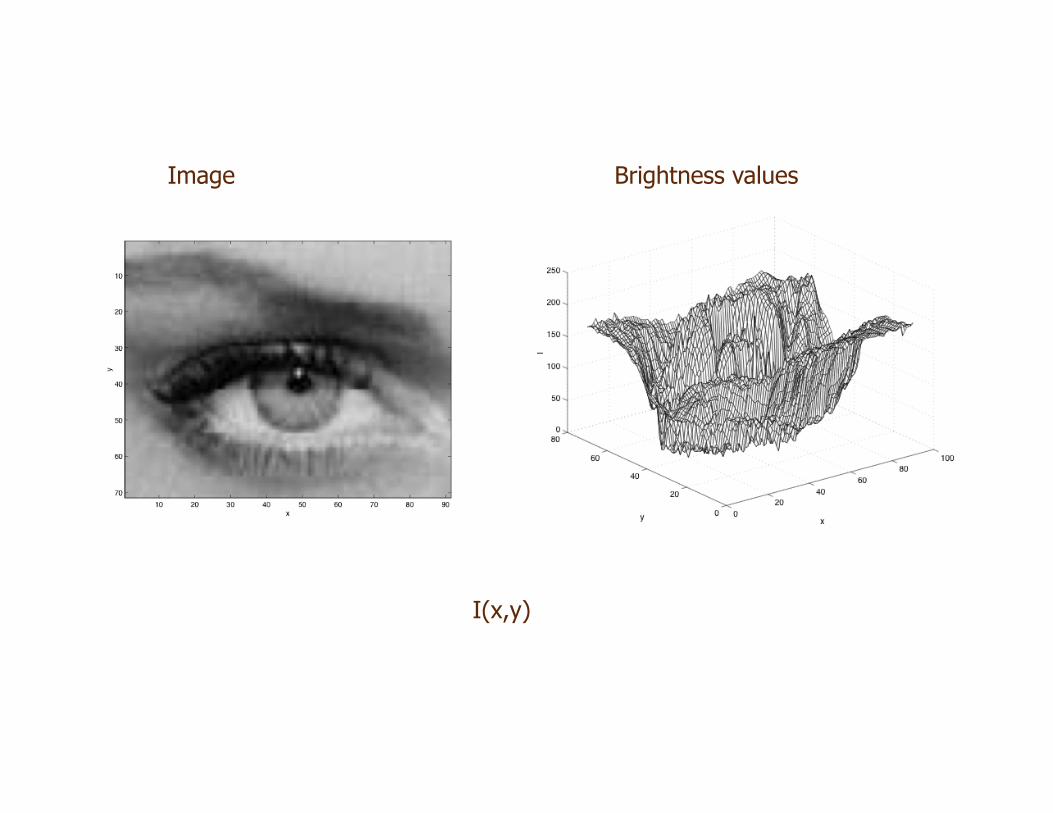
Image Brightness values
I(x,y)
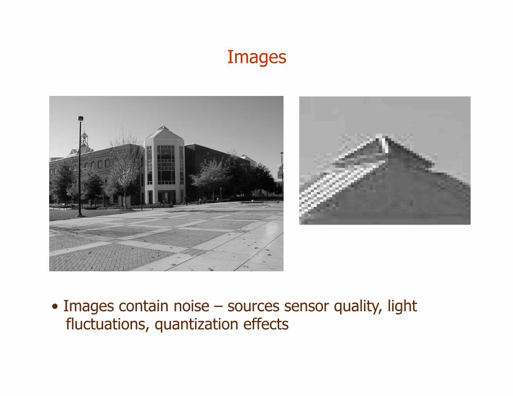
Images
• Images contain noise – sources sensor quality, light fluctuations, quantization effects
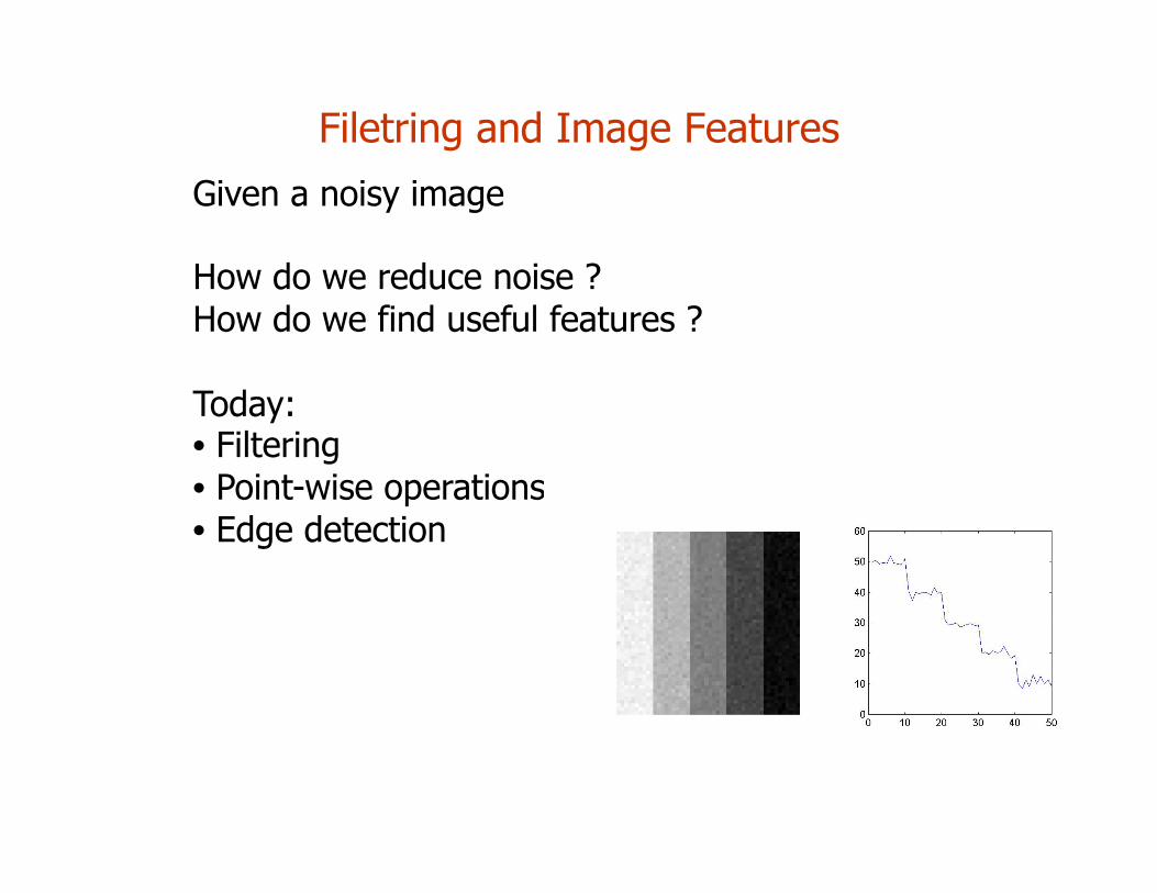
Filetring and Image Features Given a noisy image How do we reduce noise ? How do we find useful features ? Today: • Filtering • Point-wise operations • Edge detection
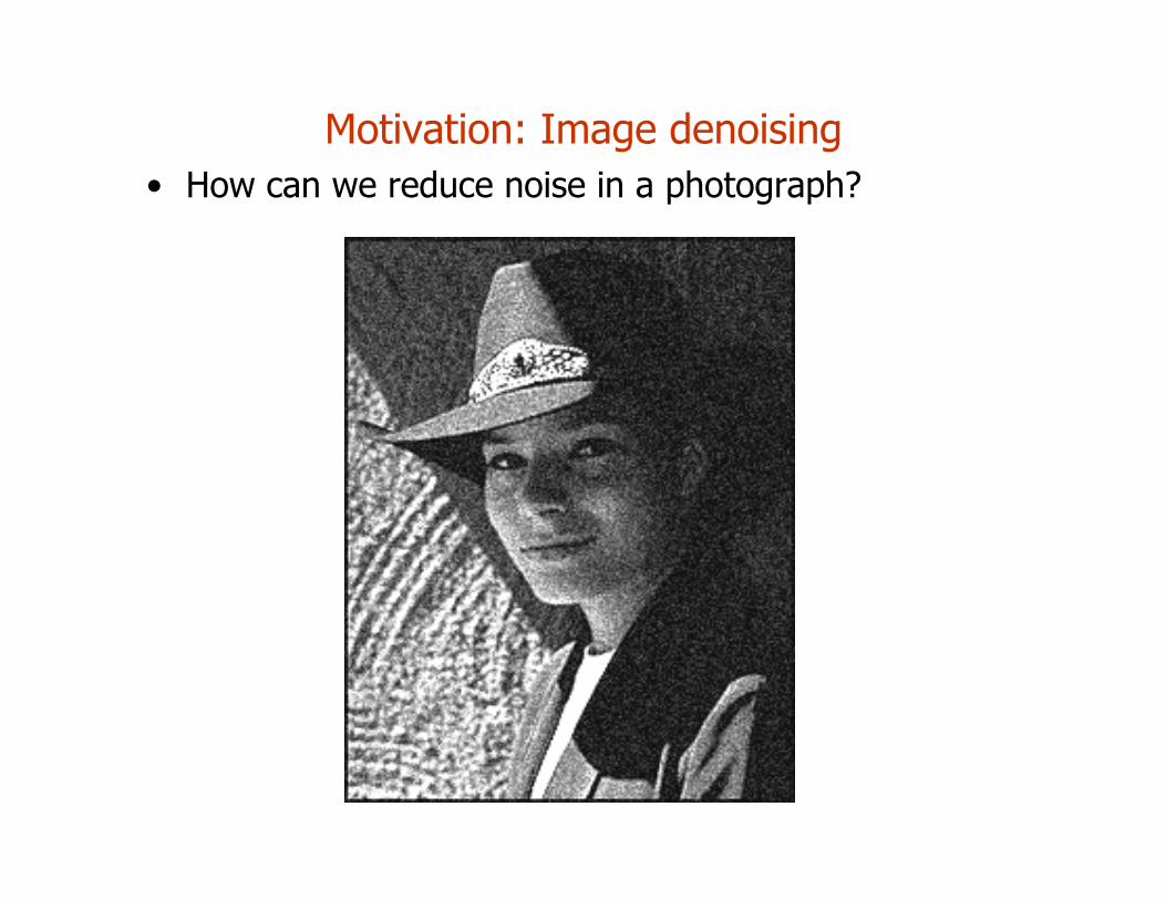
Motivation: Image denoising • How can we reduce noise in a photograph?
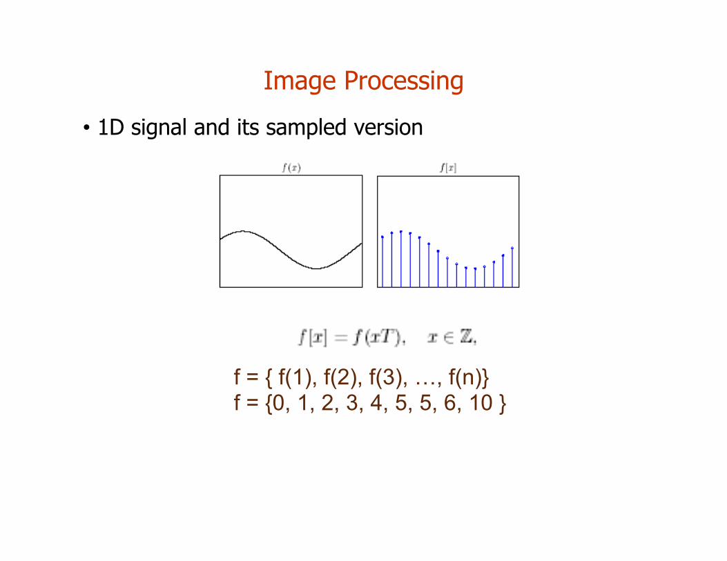
Image Processing
• 1D signal and its sampled version
f = { f(1), f(2), f(3), …, f(n)} f = {0, 1, 2, 3, 4, 5, 5, 6, 10 }
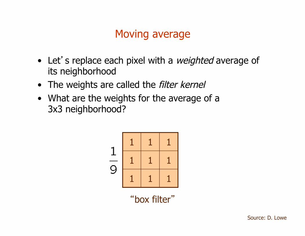
• Let’s replace each pixel with a weighted average of its neighborhood
• The weights are called the filter kernel • What are the weights for the average of a
3x3 neighborhood?
Moving average
1 1 1
1 1 1
1 1 1
“box filter”
Source: D. Lowe
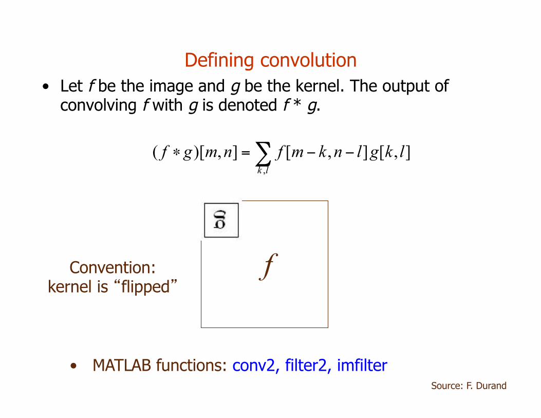
Defining convolution
f
• Let f be the image and g be the kernel. The output of convolving f with g is denoted f * g.
Source: F. Durand
• MATLAB functions: conv2, filter2, imfilter
Convention: kernel is “flipped”
8
Defining convolution
f
• Let f be the image and g be the kernel. The output of convolving f with g is denoted f * g.
Source: F. Durand
• MATLAB functions: conv2, filter2, imfilter
Convention: kernel is “flipped”
Annoying details
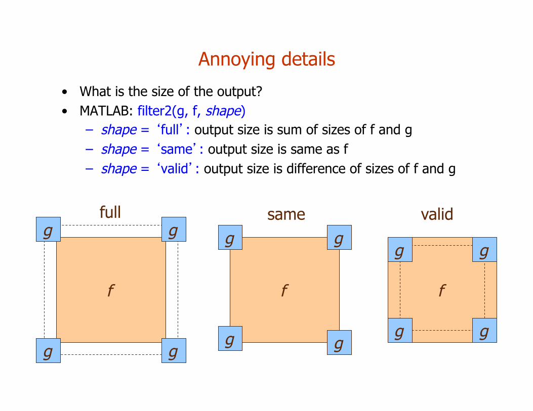
• What is the size of the output?
• MATLAB: filter2(g, f, shape)
– shape = ‘full’: output size is sum of sizes of f and g
– shape = ‘same’: output size is same as f
– shape = ‘valid’: output size is difference of sizes of f and g
f
g g
g g
f
g g
g g
f
g g
g g
full same valid
Annoying details
• What is the size of the output? • MATLAB: filter2(g, f, shape)
– shape = ‘full’: output size is sum of sizes of f and g – shape = ‘same’: output size is same as f – shape = ‘valid’: output size is difference of sizes of f and g
f
g g
g g
f
g g
g g
f
g g
g g
full same valid
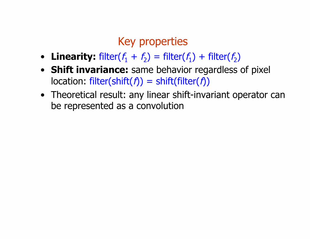
Key properties • Linearity: filter(f1 + f2) = filter(f1) + filter(f2) • Shift invariance: same behavior regardless of pixel
location: filter(shift(f)) = shift(filter(f)) • Theoretical result: any linear shift-invariant operator can
be represented as a convolution
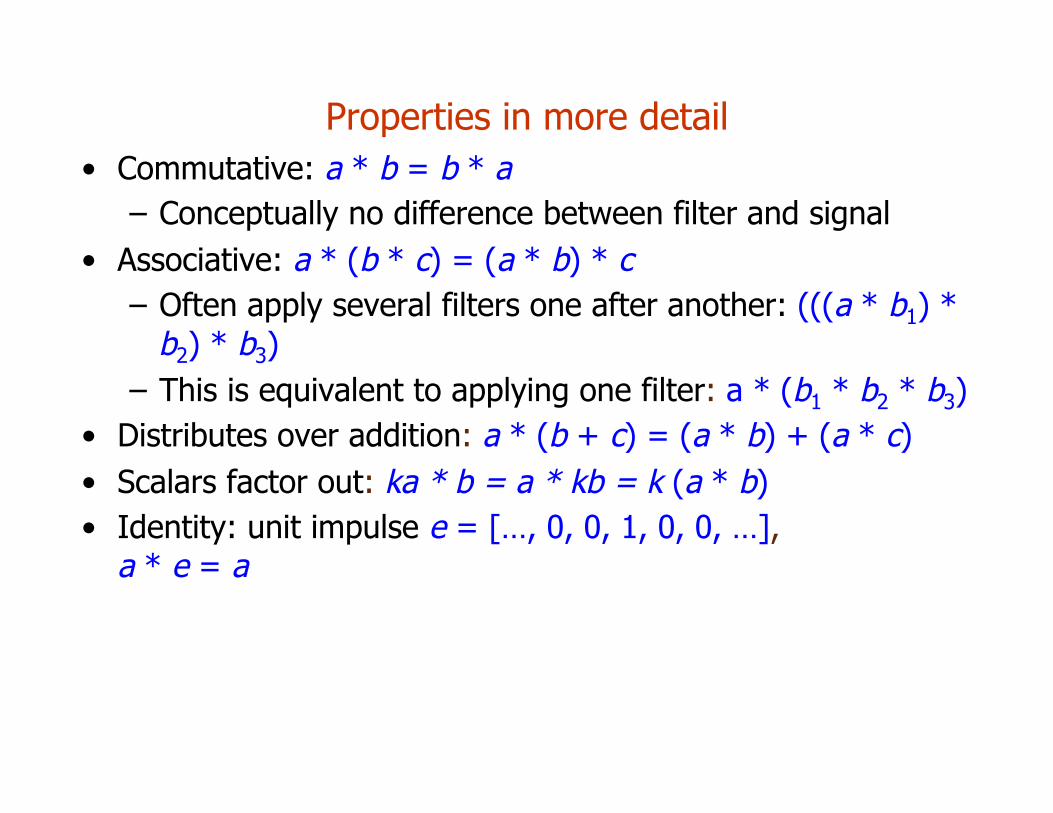
Properties in more detail • Commutative: a * b = b * a
– Conceptually no difference between filter and signal • Associative: a * (b * c) = (a * b) * c
– Often apply several filters one after another: (((a * b1) * b2) * b3)
– This is equivalent to applying one filter: a * (b1 * b2 * b3) • Distributes over addition: a * (b + c) = (a * b) + (a * c) • Scalars factor out: ka * b = a * kb = k (a * b) • Identity: unit impulse e = […, 0, 0, 1, 0, 0, …],
a * e = a
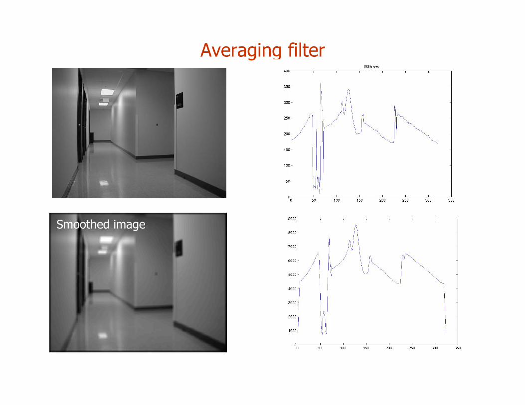
Averaging filter Original image
Smoothed image
CS223b, Jana Kosecka
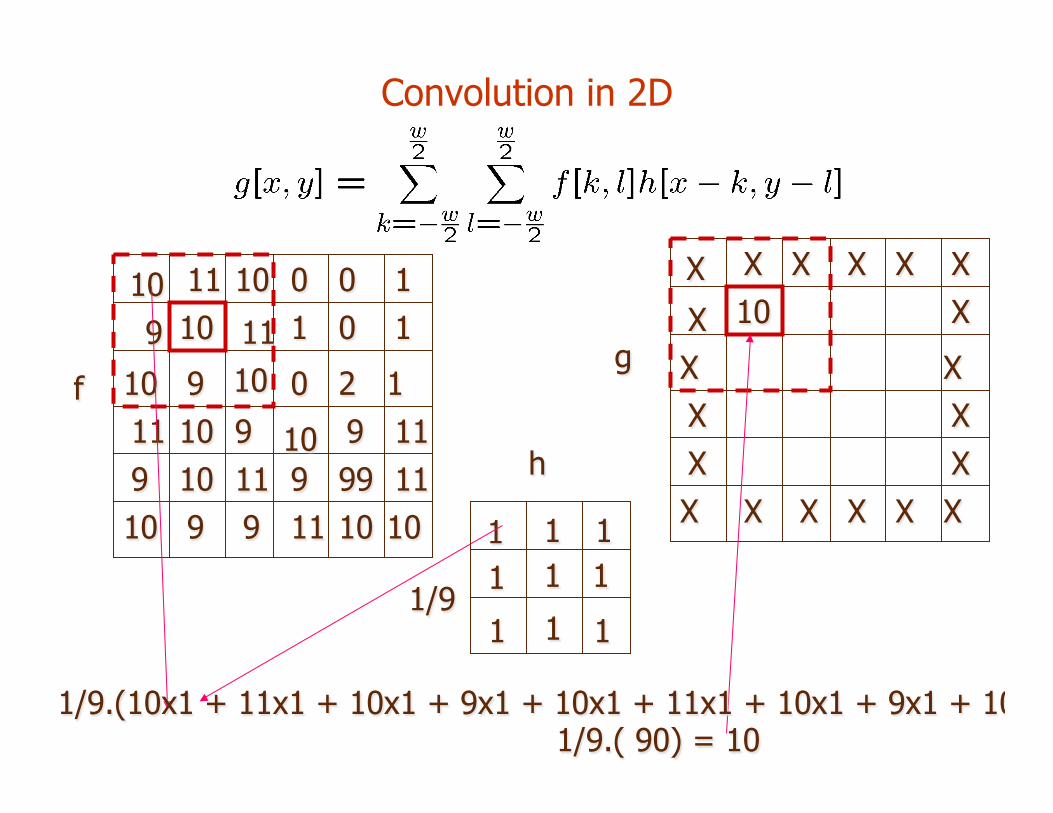
Convolution in 2D
10 11 10
9 10 11
10 9 10
1
10 10
2 9
0 9
0
9 9
9 9
0
1
99 10
10 11
1 0 1
11 11
11 11 10 10
f
1 1 1
1
1 1
1 1
1
h
X X X
X 10
X
X
X X
X
X
X
X
X
X X
X
X X X X
1/9
g
1/9.(10x1 + 11x1 + 10x1 + 9x1 + 10x1 + 11x1 + 10x1 + 9x1 + 10x1) = 1/9.( 90) = 10
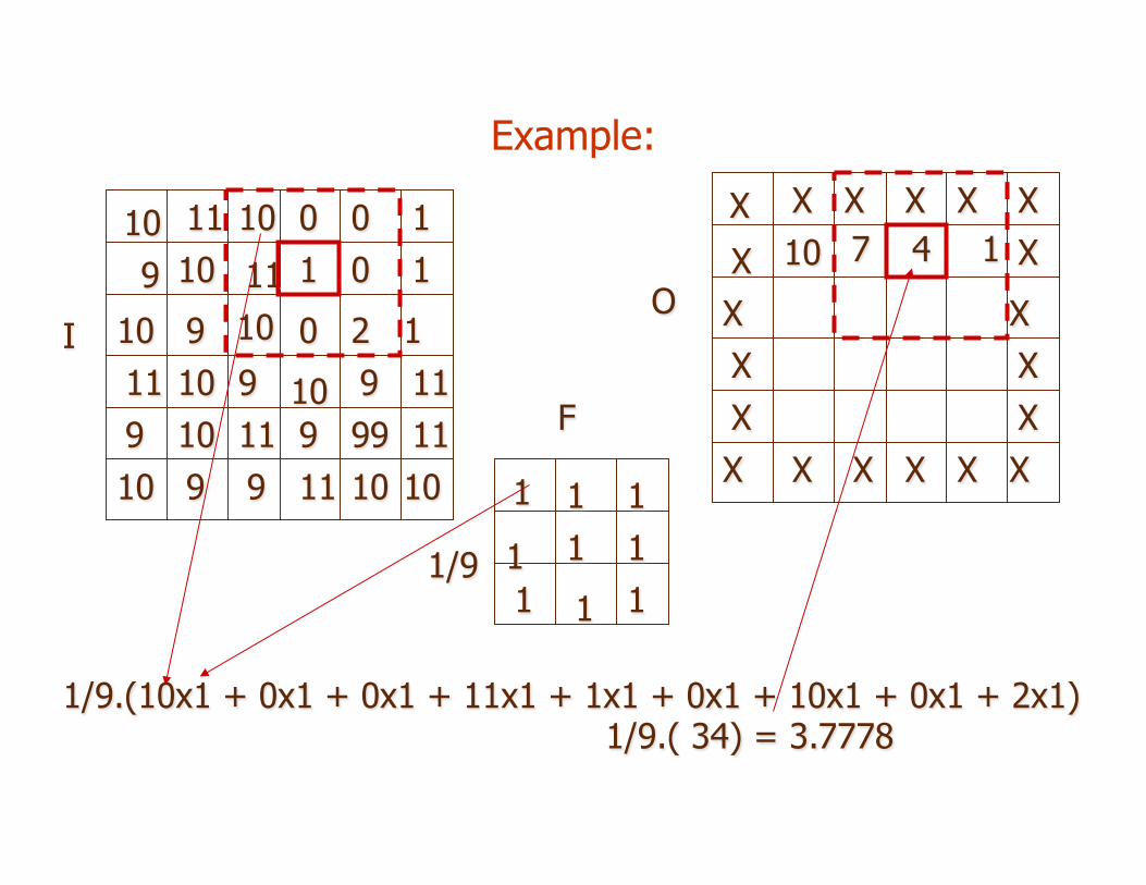
Example:
1/9.(10x1 + 0x1 + 0x1 + 11x1 + 1x1 + 0x1 + 10x1 + 0x1 + 2x1) = 1/9.( 34) = 3.7778
10 11 10
9 10 11
10 9 10
1
10 10
2 9
0 9
0
9 9
9 9
0
1
99 10
10 11
1 0 1
11 11
11 11 10 10
I
1
1 1
1 1 1
1 1
1
F
X X X
X 10
X
X
X X
X
X
X
X
X
X X
X
X X X X
1/9
O 4 7 1
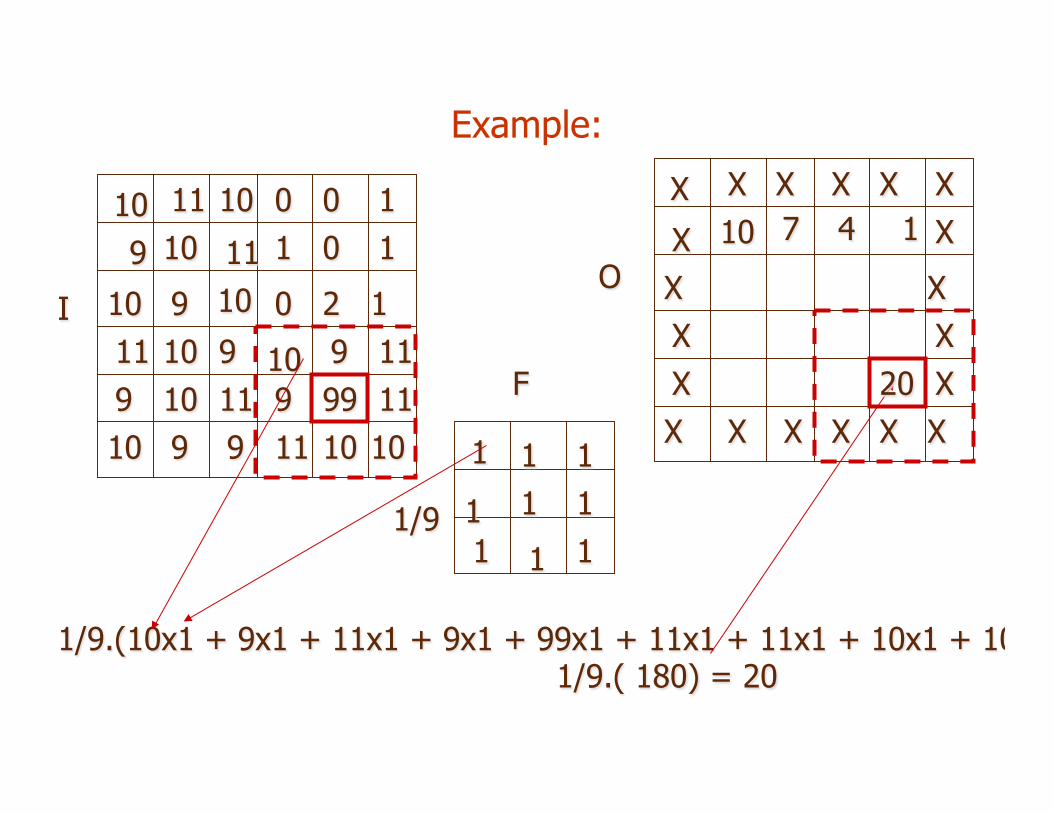
Example:
1/9.(10x1 + 9x1 + 11x1 + 9x1 + 99x1 + 11x1 + 11x1 + 10x1 + 10x1) = 1/9.( 180) = 20
10 11 10
9 10 11
10 9 10
1
10 10
2 9
0 9
0
9 9
9 9
0
1
99 10
10 11
1 0 1
11 11
11 11 10 10
I
1
1 1
1 1 1
1 1
1
F
X X X
X 10
X
X
X X
X
X
X
X
X
X X
X
X X X X
1/9
O 4 7 1
20
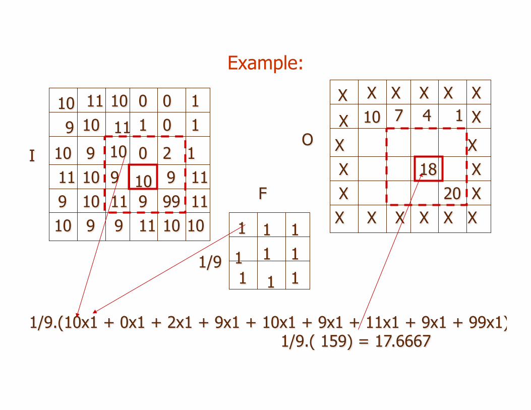
Example:
1/9.(10x1 + 0x1 + 2x1 + 9x1 + 10x1 + 9x1 + 11x1 + 9x1 + 99x1) = 1/9.( 159) = 17.6667
10 11 10
9 10 11
10 9 10
1
10 10
2 9
0 9
0
9 9
9 9
0
1
99 10
10 11
1 0 1
11 11
11 11 10 10
I
1
1 1
1 1 1
1 1
1
F
X X X
X 10
X
X
X X
X
X
X
X
X
X X
X
X X X X
1/9
O 4 7 1
18 20
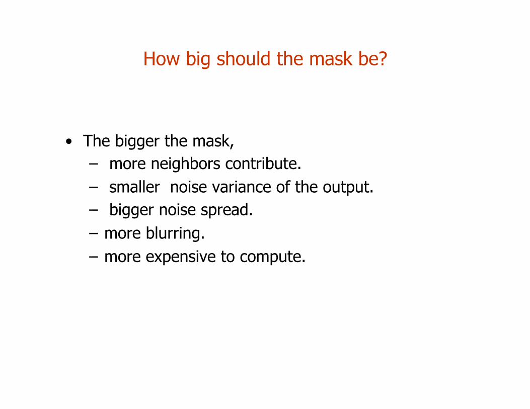
How big should the mask be?
• The bigger the mask, – more neighbors contribute. – smaller noise variance of the output. – bigger noise spread. – more blurring. – more expensive to compute.
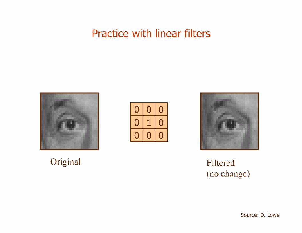
Practice with linear filters
0 0 0 0 1 0 0 0 0
Original Filtered (no change)
Source: D. Lowe
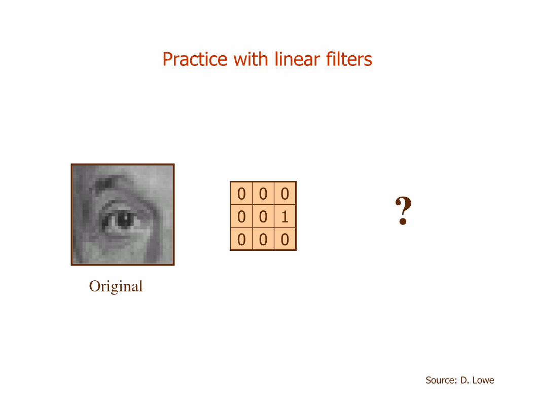
Practice with linear filters
0 0 0 1 0 0 0 0 0
Original
?
Source: D. Lowe
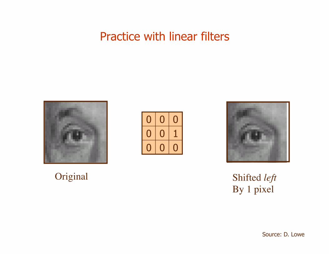
Practice with linear filters
0 0 0 1 0 0 0 0 0
Original Shifted leftBy 1 pixel
Source: D. Lowe
Practice with linear filters
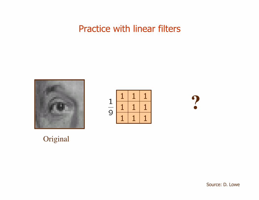
Original
?1 1 1 1 1 1 1 1 1
Source: D. Lowe
Practice with linear filters
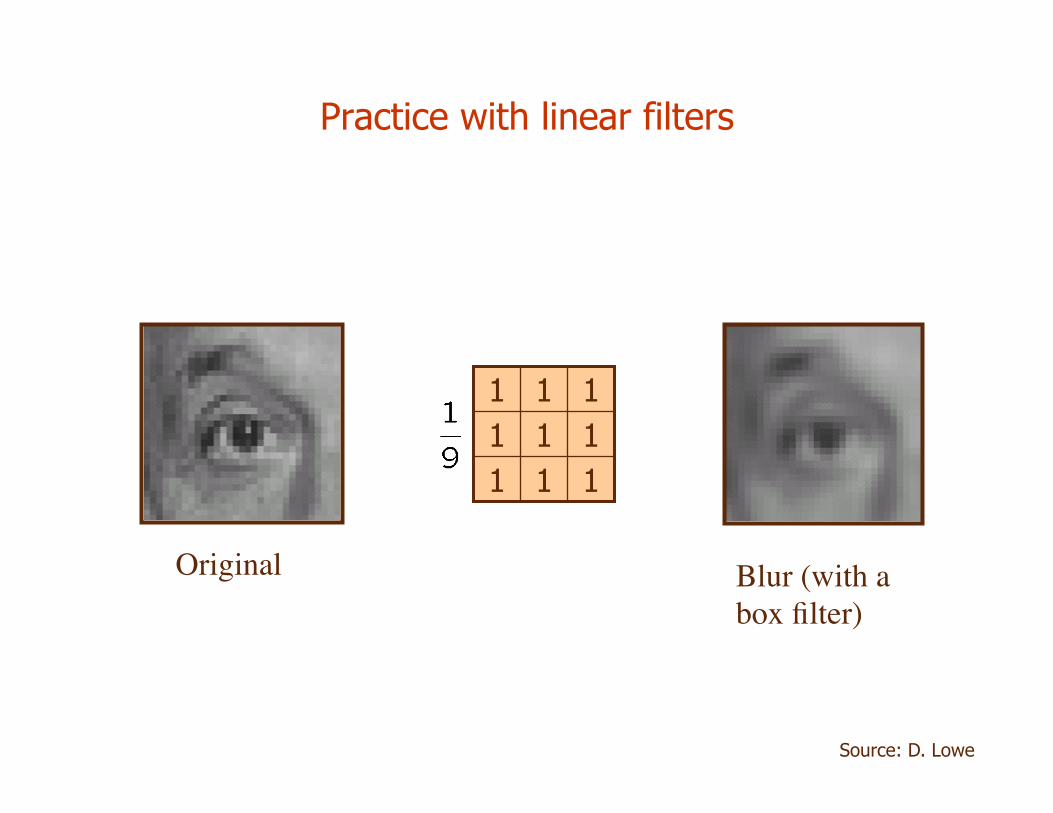
Original
1 1 1 1 1 1 1 1 1
Blur (with abox filter)
Source: D. Lowe
Practice with linear filters
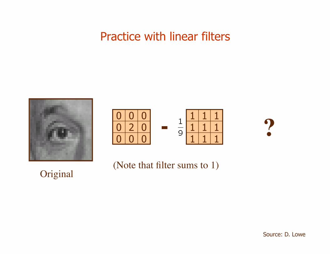
Original
1 1 1 1 1 1 1 1 1
0 0 0 0 2 0 0 0 0 - ?
(Note that filter sums to 1)
Source: D. Lowe
Practice with linear filters
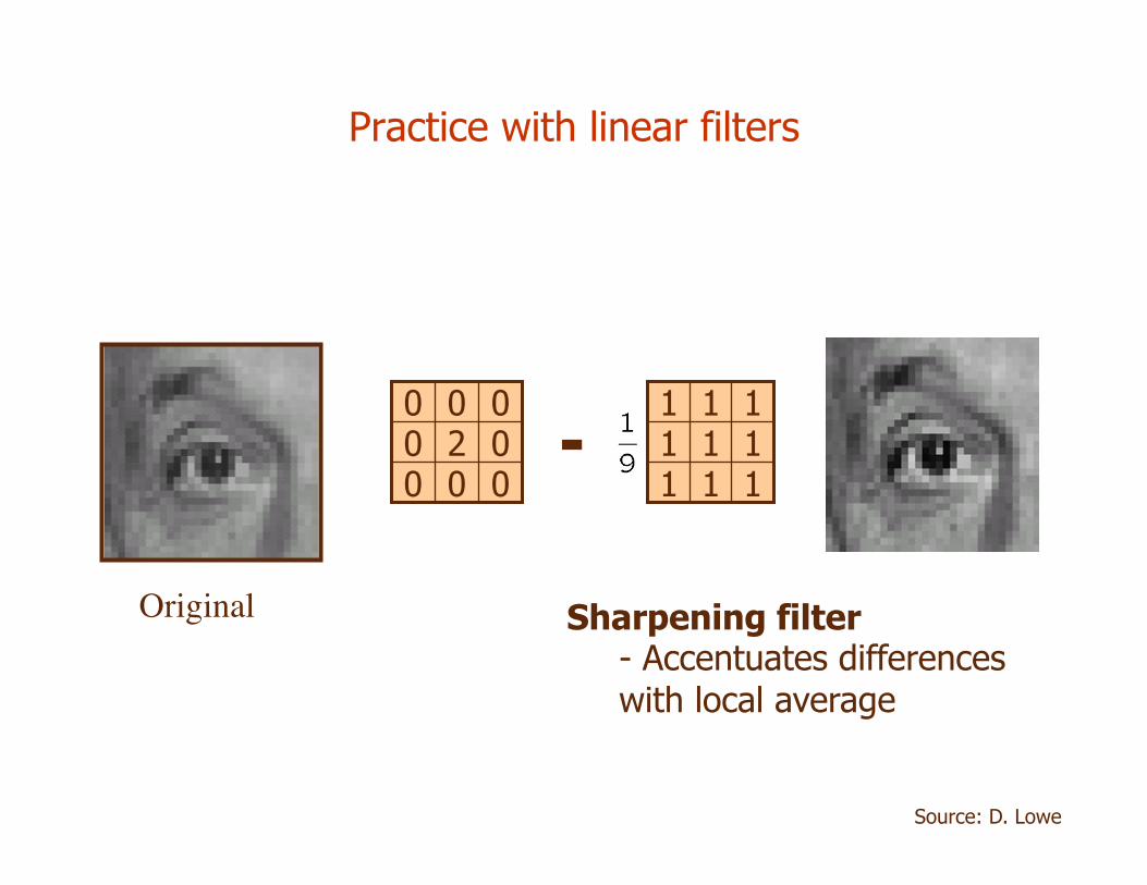
Original
1 1 1 1 1 1 1 1 1
0 0 0 0 2 0 0 0 0 -
Sharpening filter - Accentuates differences with local average
Source: D. Lowe
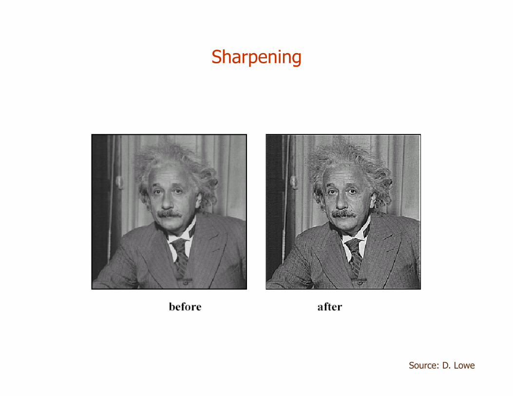
Sharpening
Source: D. Lowe
Computer Vision - A Modern Approach
Set: Linear Filters Slides by D.A. Forsyth
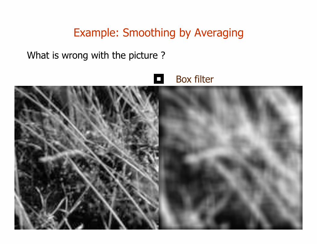
Example: Smoothing by Averaging
Box filter
What is wrong with the picture ?
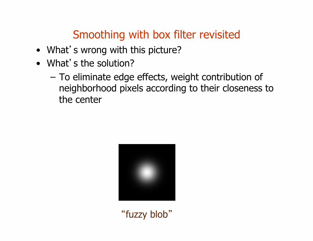
Smoothing with box filter revisited • What’s wrong with this picture? • What’s the solution?
– To eliminate edge effects, weight contribution of neighborhood pixels according to their closeness to the center
“fuzzy blob”
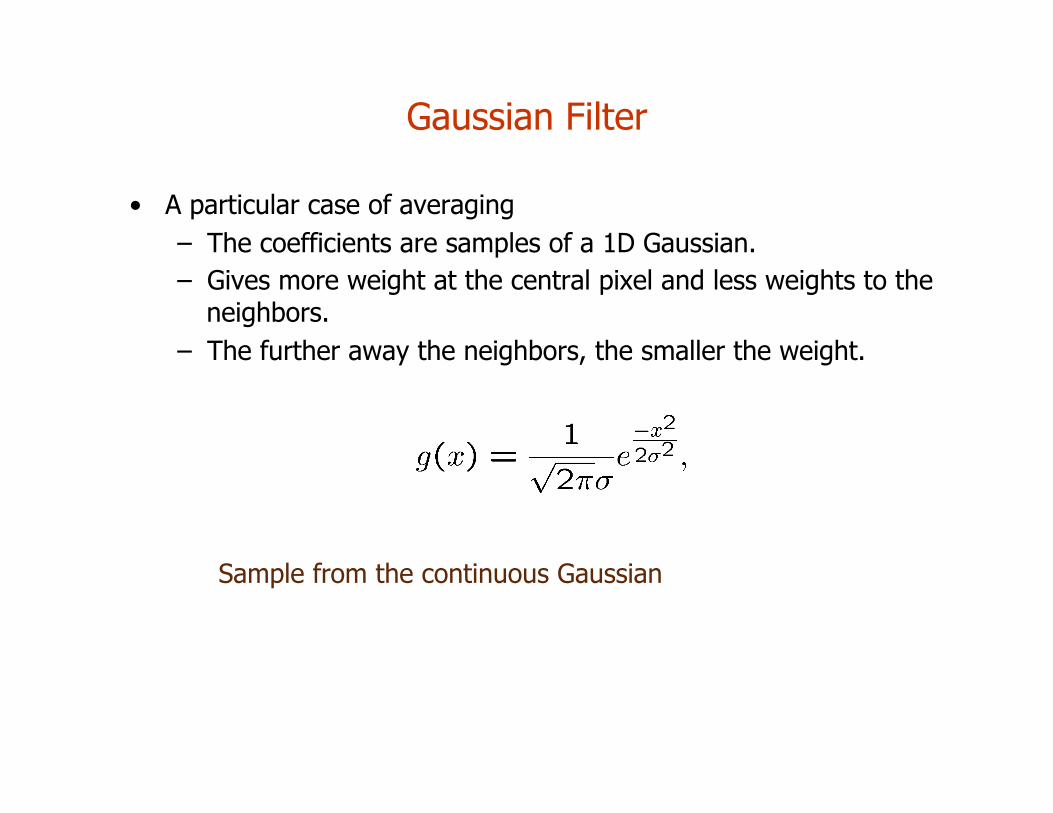
Gaussian Filter
• A particular case of averaging – The coefficients are samples of a 1D Gaussian. – Gives more weight at the central pixel and less weights to the
neighbors. – The further away the neighbors, the smaller the weight.
Sample from the continuous Gaussian
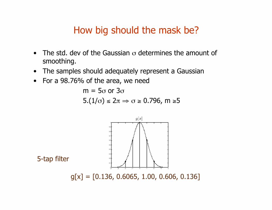
How big should the mask be?
• The std. dev of the Gaussian σ determines the amount of smoothing.
• The samples should adequately represent a Gaussian • For a 98.76% of the area, we need
m = 5σ or 3σ 5.(1/σ) ≤ 2π ⇒ σ ≥ 0.796, m ≥5
g[x] = [0.136, 0.6065, 1.00, 0.606, 0.136]
5-tap filter
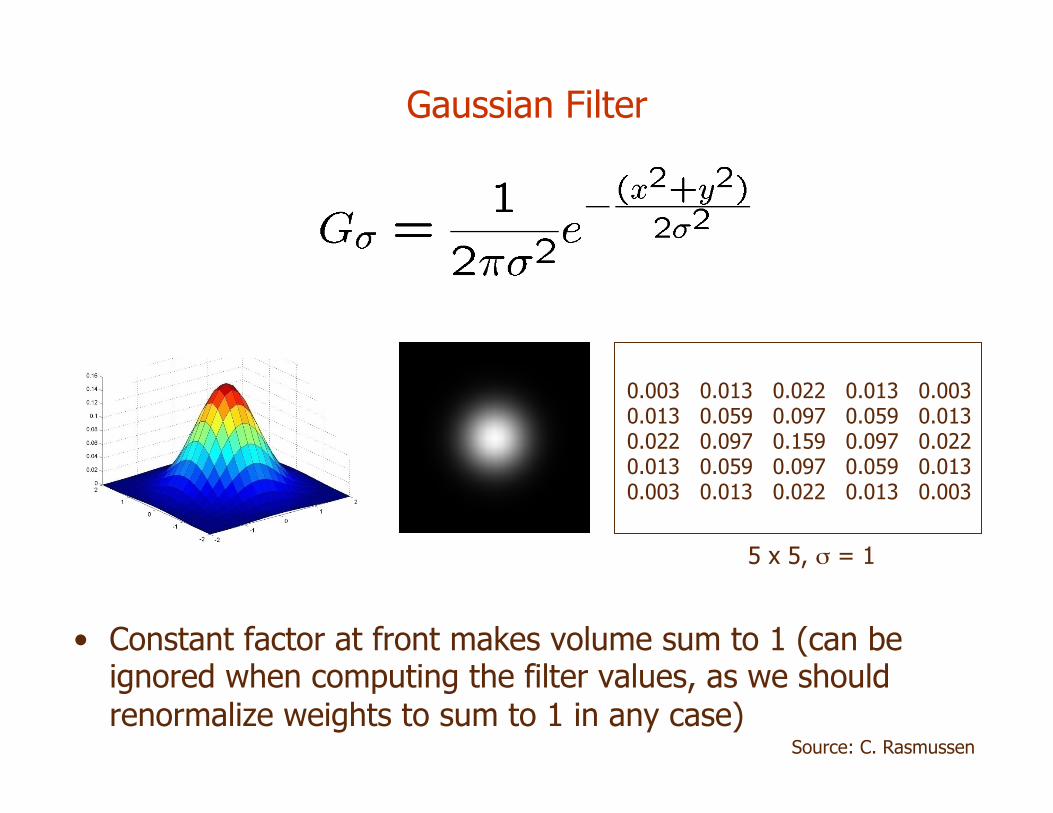
Gaussian Filter
• Constant factor at front makes volume sum to 1 (can be ignored when computing the filter values, as we should renormalize weights to sum to 1 in any case)
0.003 0.013 0.022 0.013 0.003 0.013 0.059 0.097 0.059 0.013 0.022 0.097 0.159 0.097 0.022 0.013 0.059 0.097 0.059 0.013 0.003 0.013 0.022 0.013 0.003
5 x 5, σ = 1
Source: C. Rasmussen
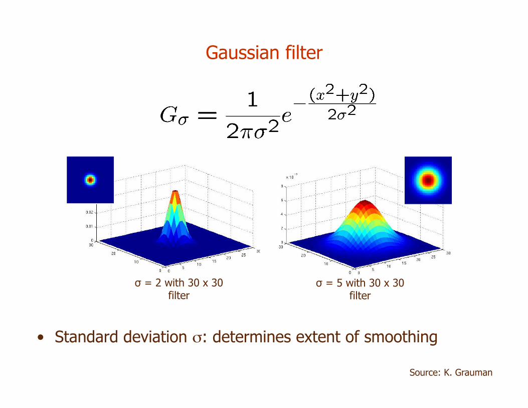
Gaussian filter
• Standard deviation σ: determines extent of smoothing
Source: K. Grauman
σ = 2 with 30 x 30 filter
σ = 5 with 30 x 30 filter
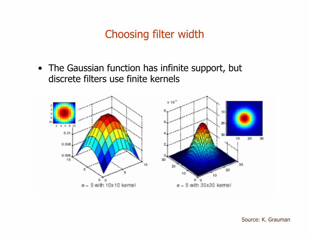
Choosing filter width
• The Gaussian function has infinite support, but discrete filters use finite kernels
Source: K. Grauman
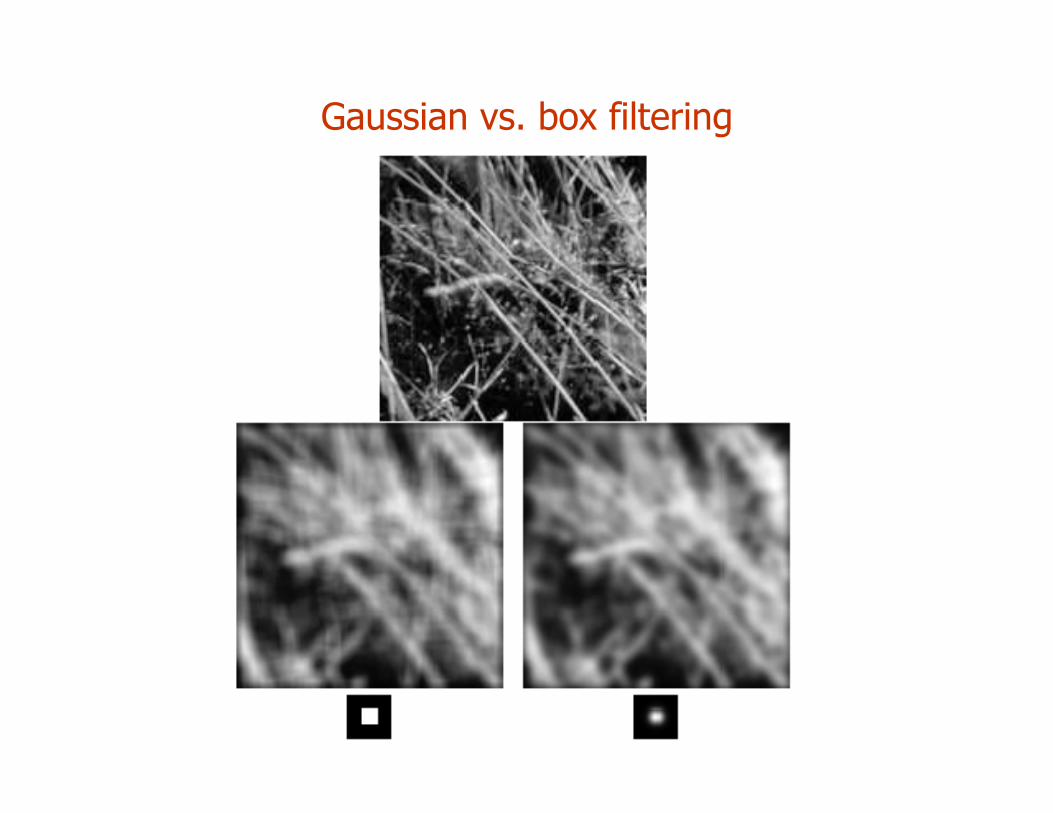
Gaussian vs. box filtering
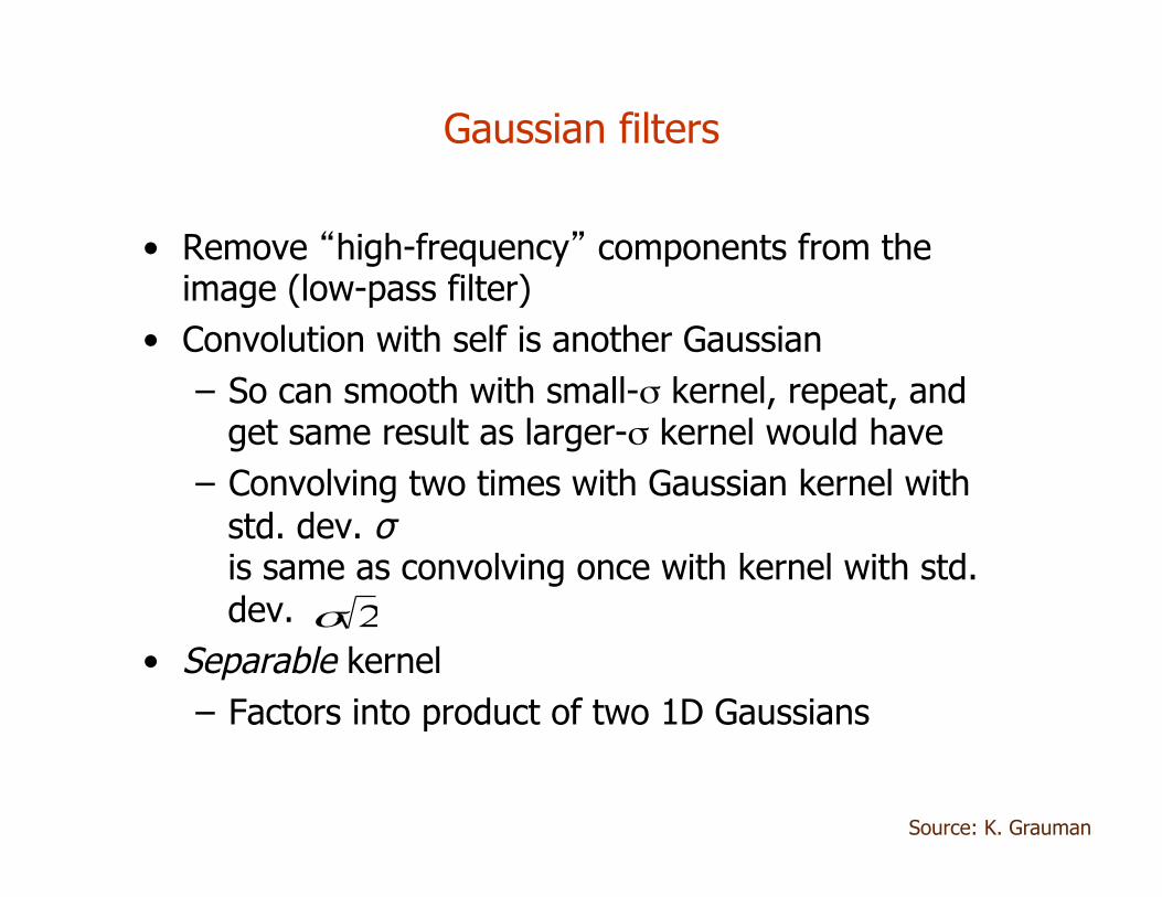
Gaussian filters
• Remove “high-frequency” components from the image (low-pass filter)
• Convolution with self is another Gaussian – So can smooth with small-σ kernel, repeat, and
get same result as larger-σ kernel would have – Convolving two times with Gaussian kernel with
std. dev. σ is same as convolving once with kernel with std. dev.
• Separable kernel – Factors into product of two 1D Gaussians
Source: K. Grauman
2σ
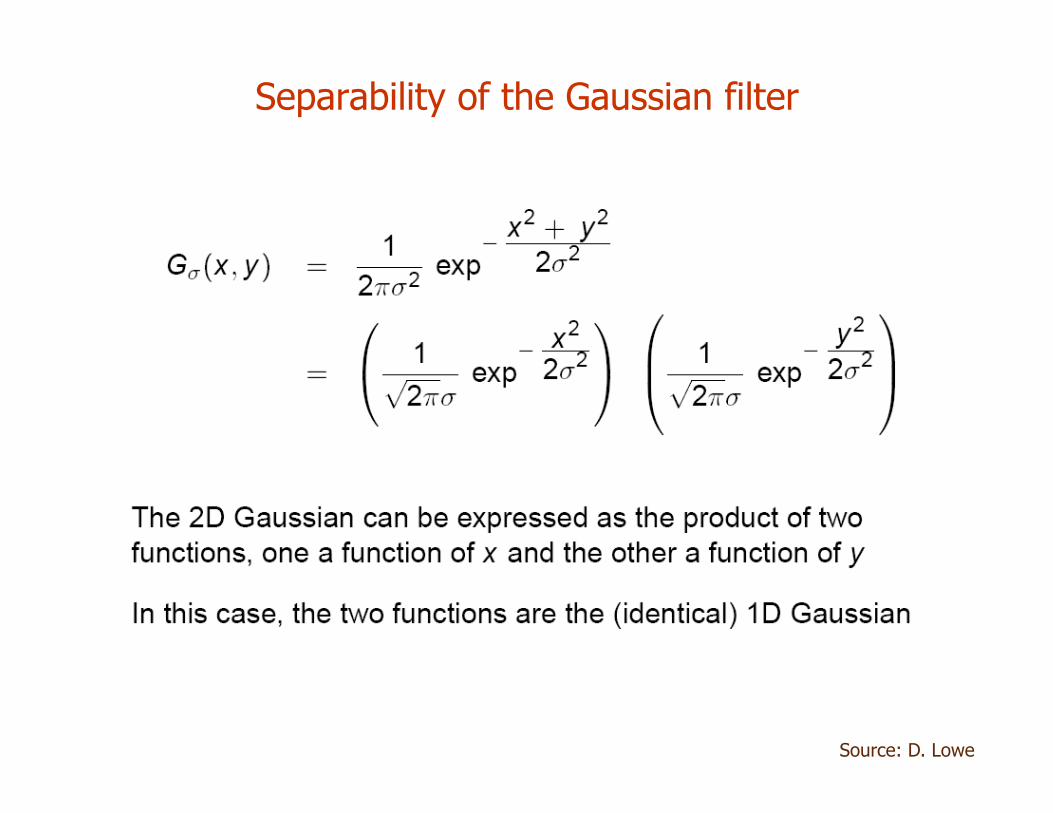
Separability of the Gaussian filter
Source: D. Lowe
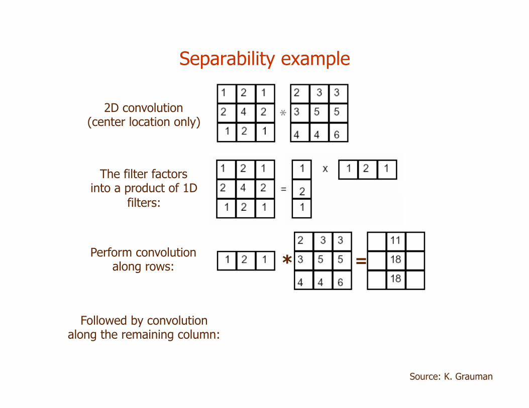
Separability example
*
*
=
=
2D convolution (center location only)
Source: K. Grauman
The filter factors into a product of 1D
filters:
Perform convolution along rows:
Followed by convolution along the remaining column:
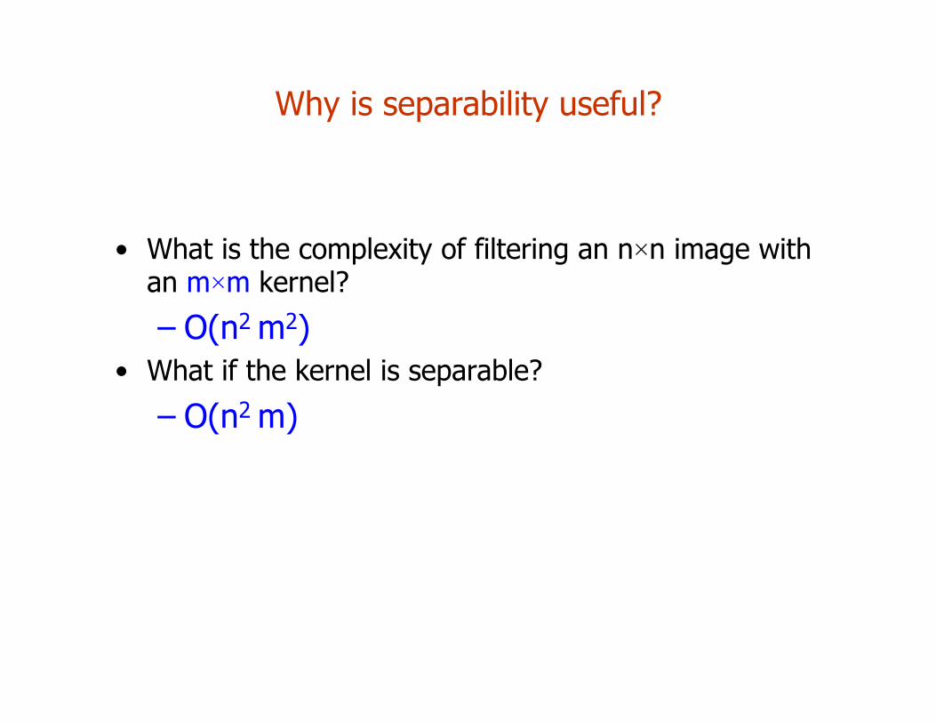
Why is separability useful?
• What is the complexity of filtering an n×n image with an m×m kernel?
– O(n2 m2) • What if the kernel is separable?
– O(n2 m)
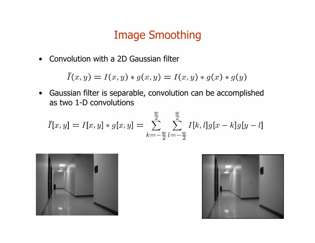
Image Smoothing
• Convolution with a 2D Gaussian filter
• Gaussian filter is separable, convolution can be accomplished as two 1-D convolutions
Non-linear Filtering
• Replace each pixel with the MEDIAN value of all the pixels in the neighborhood.
• Non-linear • Does not spread the noise • Can remove spike noise • Expensive to run
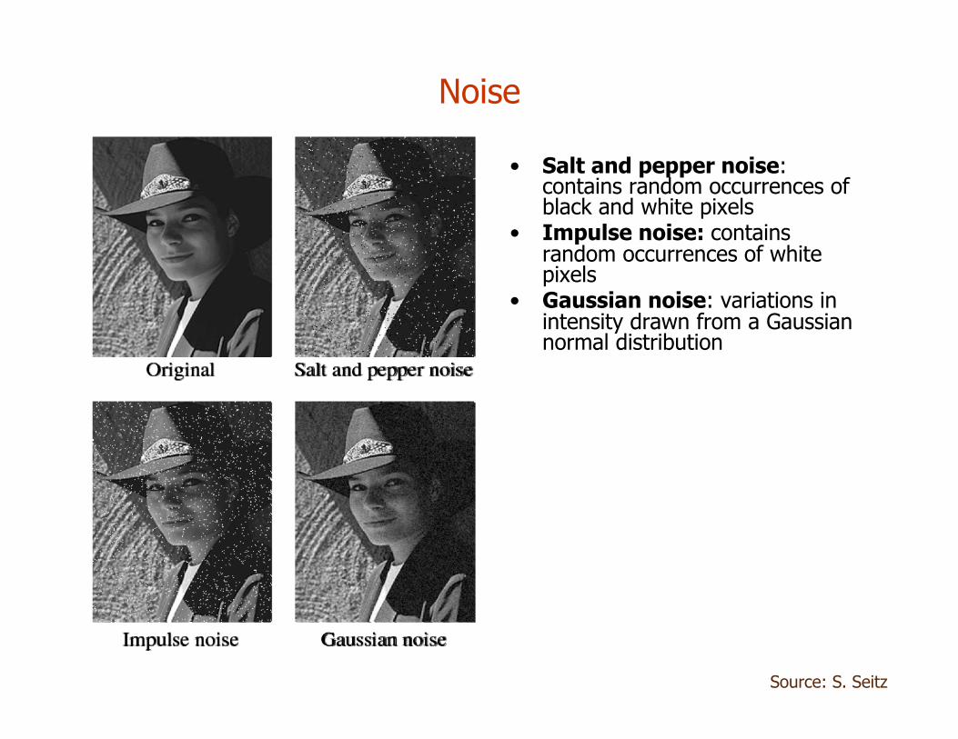
Noise
• Salt and pepper noise: contains random occurrences of black and white pixels
• Impulse noise: contains random occurrences of white pixels
• Gaussian noise: variations in intensity drawn from a Gaussian normal distribution
Source: S. Seitz
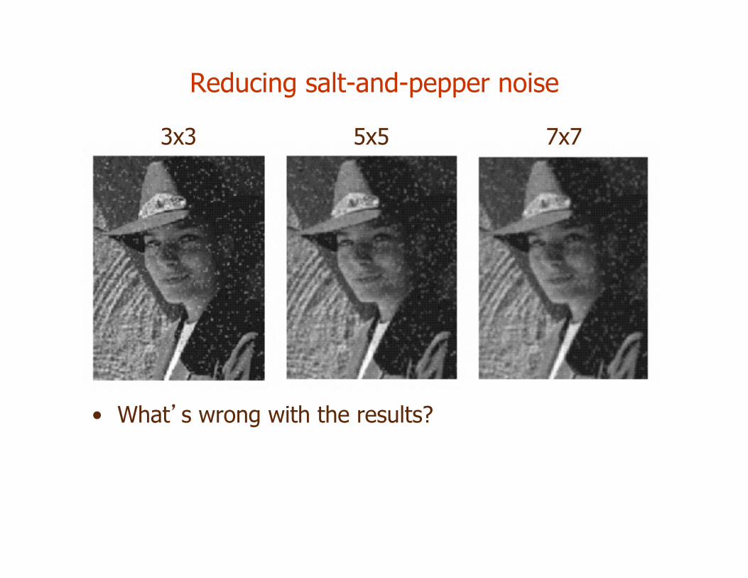
Reducing salt-and-pepper noise
• What’s wrong with the results?
3x3 5x5 7x7
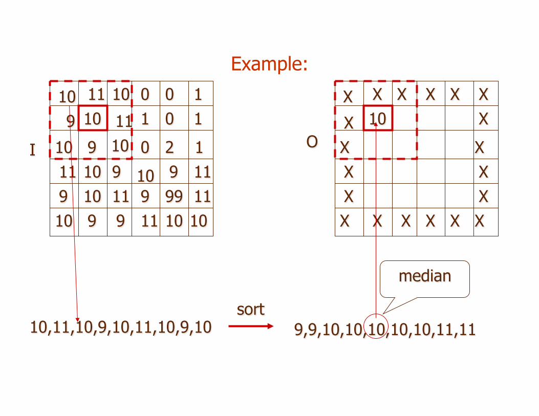
Example:
10,11,10,9,10,11,10,9,10
10 11 10
9 10 11
10 9 10
1
10 10
2 9
0 9
0
9 9
9 9
0
1
99 10
10 11
1 0 1
11 11
11 11 10 10
I
X X X
X 10
X
X
X X
X
X
X
X
X
X X
X
X X X X
O
9,9,10,10,10,10,10,11,11 sort
median
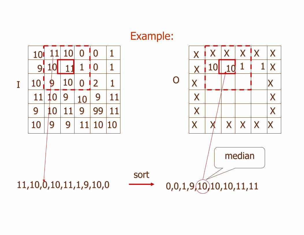
Example:
11,10,0,10,11,1,9,10,0
10 11 10
9 10 11
10 9 10
1
10 10
2 9
0 9
0
9 9
9 9
0
1
99 10
10 11
1 0 1
11 11
11 11 10 10
I
X X X
X 10
X
X
X X
X
X
X
X
X
X X
X
X X X X
O
0,0,1,9,10,10,10,11,11 sort
median
10 1 1
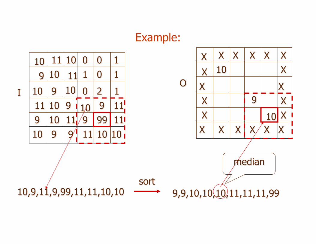
Example:
10,9,11,9,99,11,11,10,10
10 11 10
9 10 11
10 9 10
1
10 10
2 9
0 9
0
9 9
9 9
0
1
99 10
10 11
1 0 1
11 11
11 11 10 10
I
X X X
X 10
X
X
X X
X
X
X
X
X
X X
X
X X X X
O
9,9,10,10,10,11,11,11,99 sort
median
10
9
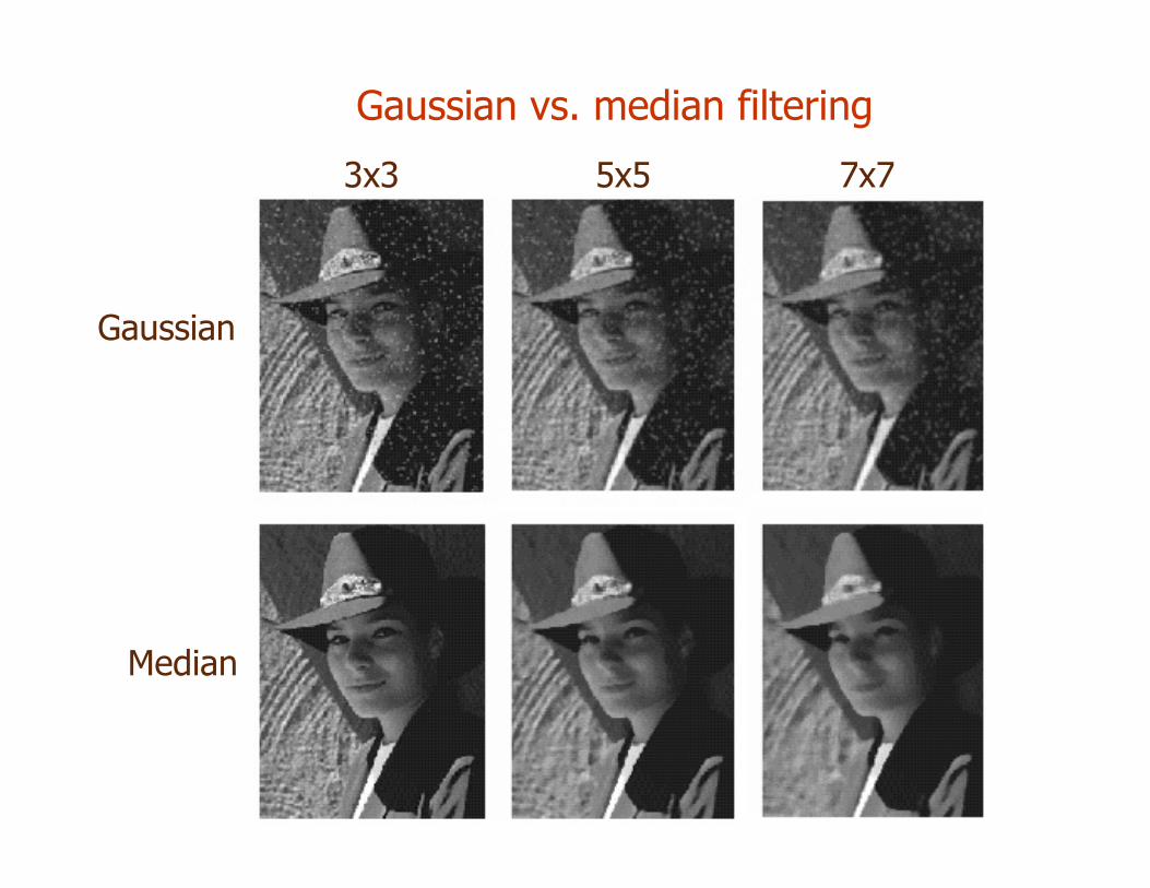
Gaussian vs. median filtering
3x3 5x5 7x7
Gaussian
Median
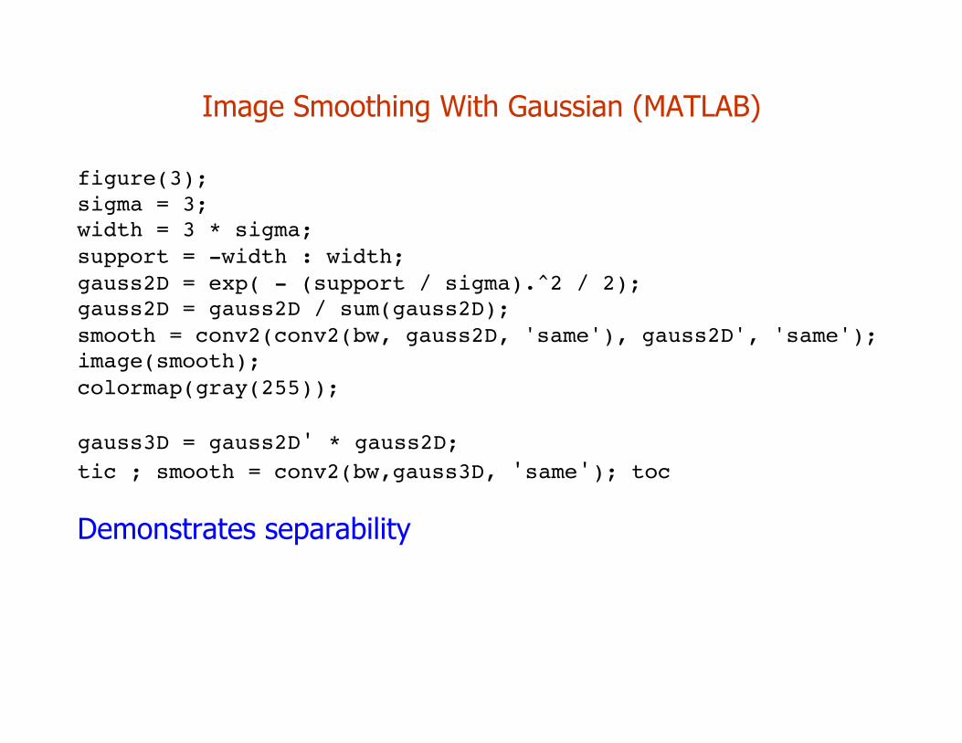
Image Smoothing With Gaussian (MATLAB)
figure(3);sigma = 3;width = 3 * sigma;support = -width : width;gauss2D = exp( - (support / sigma).^2 / 2); gauss2D = gauss2D / sum(gauss2D);smooth = conv2(conv2(bw, gauss2D, 'same'), gauss2D', 'same');image(smooth);colormap(gray(255));
gauss3D = gauss2D' * gauss2D;tic ; smooth = conv2(bw,gauss3D, 'same'); toc
Demonstrates separability
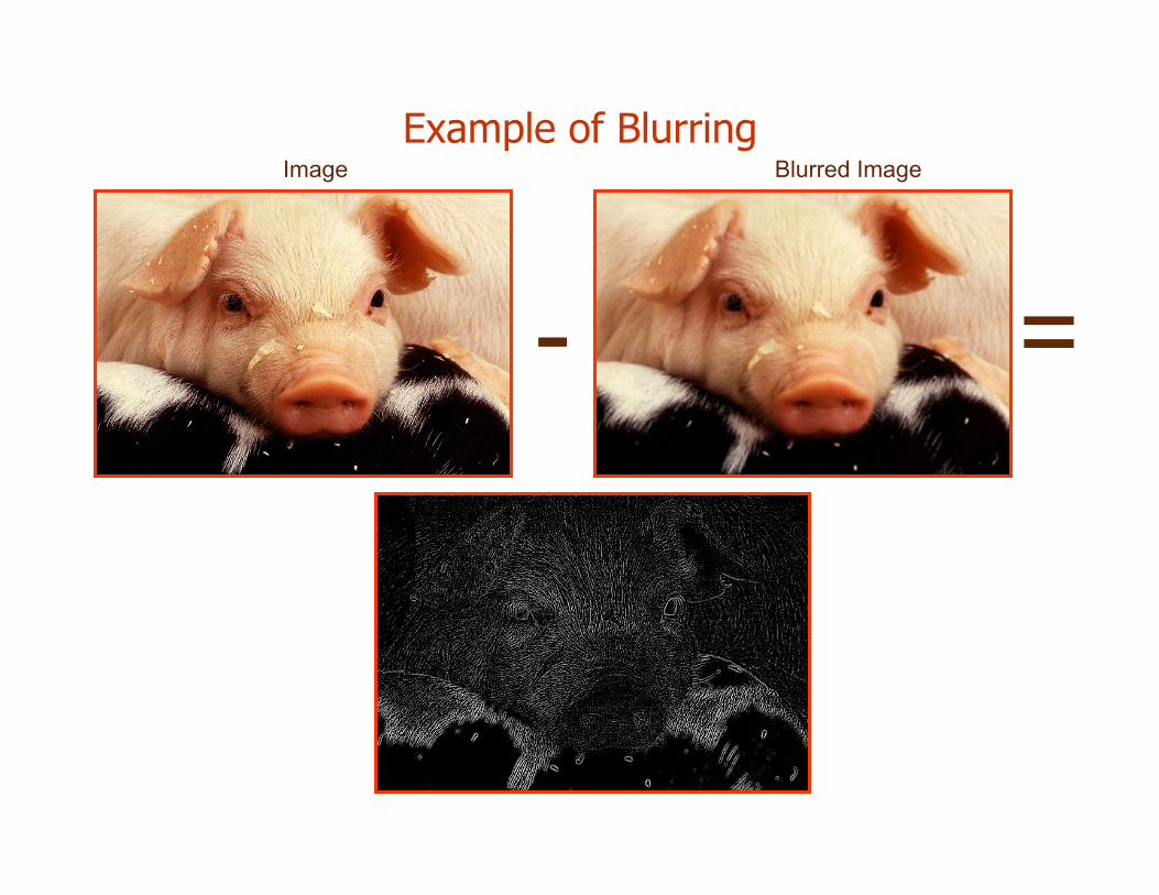
Example of Blurring Image Blurred Image
- =
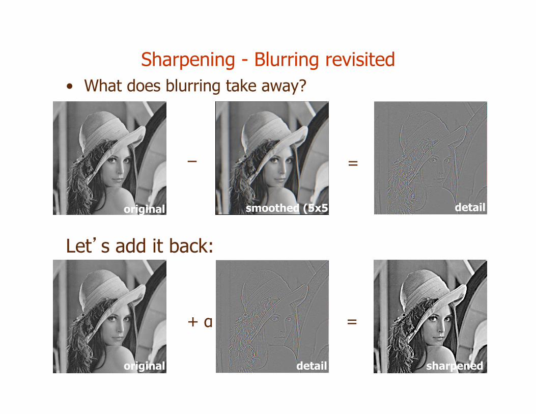
Sharpening - Blurring revisited • What does blurring take away?
original smoothed (5x5)
–
detail
=
sharpened
=
Let’s add it back:
original detail
+ α
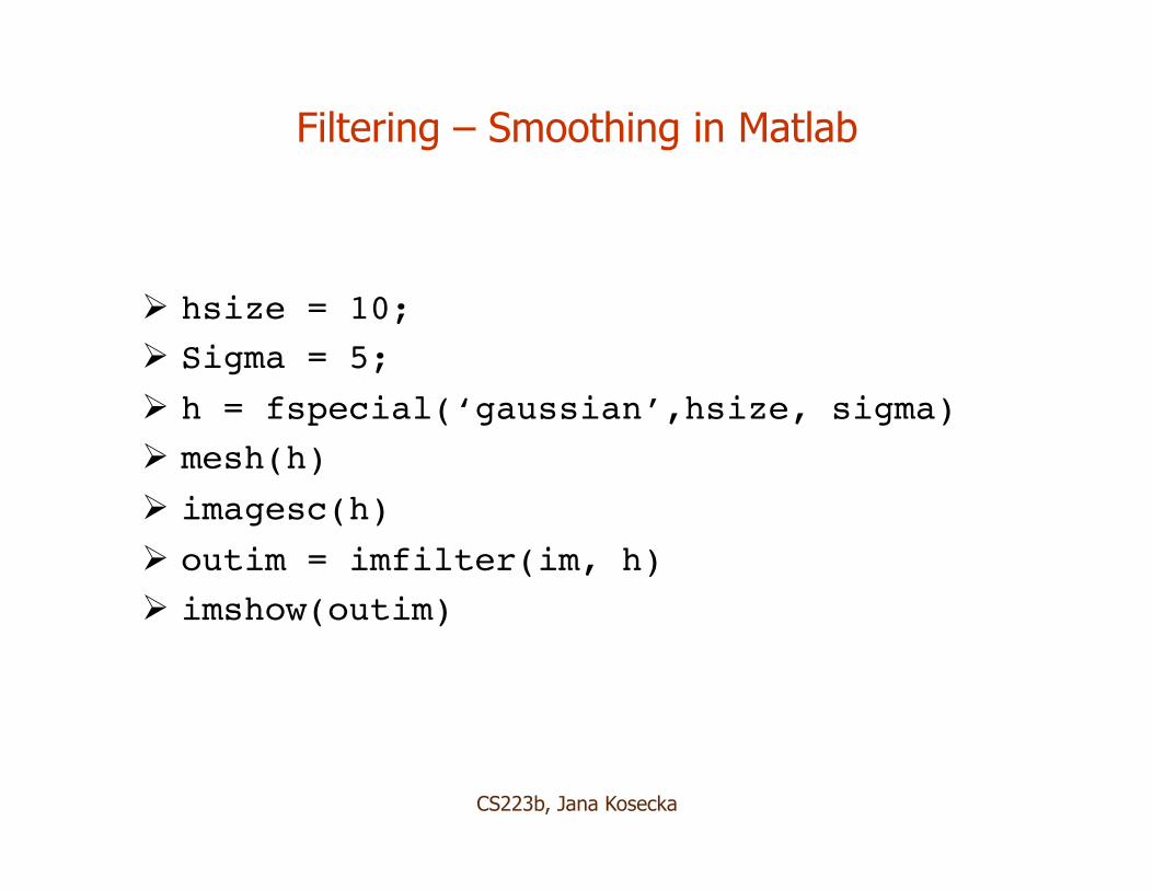
Filtering – Smoothing in Matlab
! hsize = 10; ! Sigma = 5; ! h = fspecial(‘gaussian’,hsize, sigma)! mesh(h)! imagesc(h)! outim = imfilter(im, h)! imshow(outim)
CS223b, Jana Kosecka
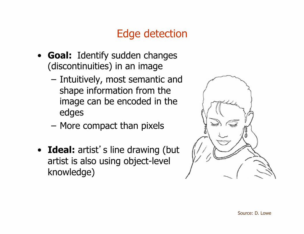
Edge detection
• Goal: Identify sudden changes (discontinuities) in an image – Intuitively, most semantic and
shape information from the image can be encoded in the edges
– More compact than pixels
• Ideal: artist’s line drawing (but artist is also using object-level knowledge)
Source: D. Lowe
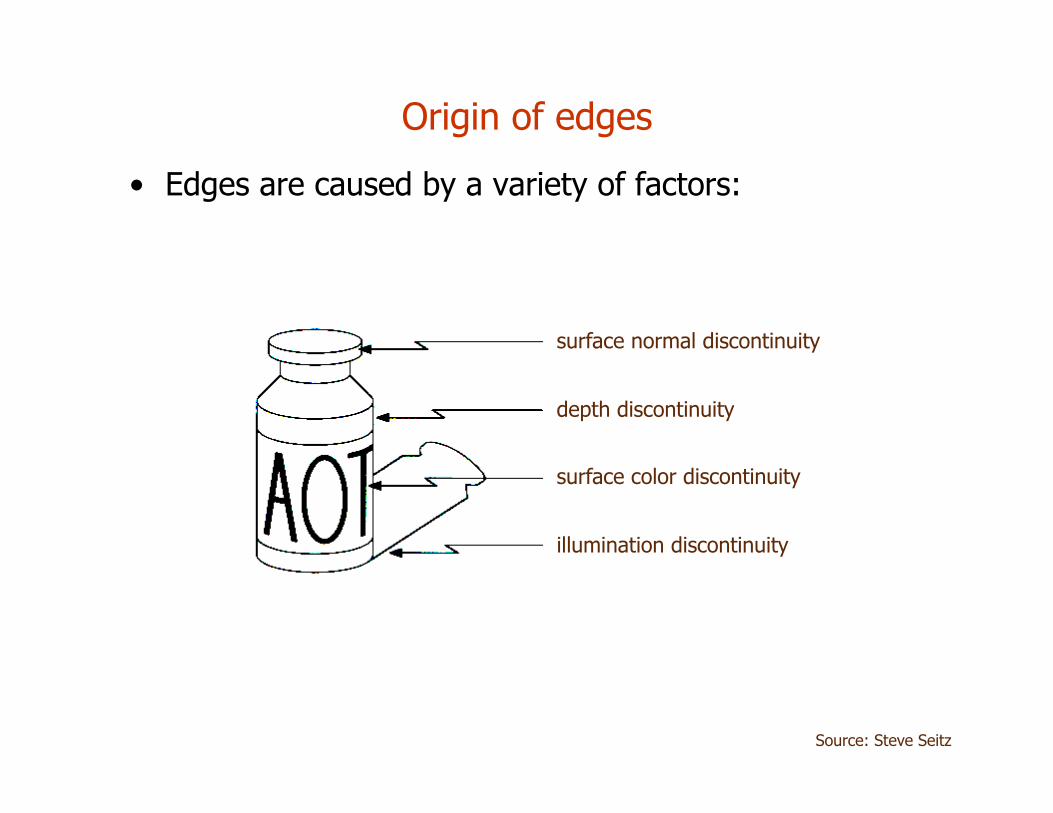
Origin of edges
• Edges are caused by a variety of factors:
depth discontinuity
surface color discontinuity
illumination discontinuity
surface normal discontinuity
Source: Steve Seitz
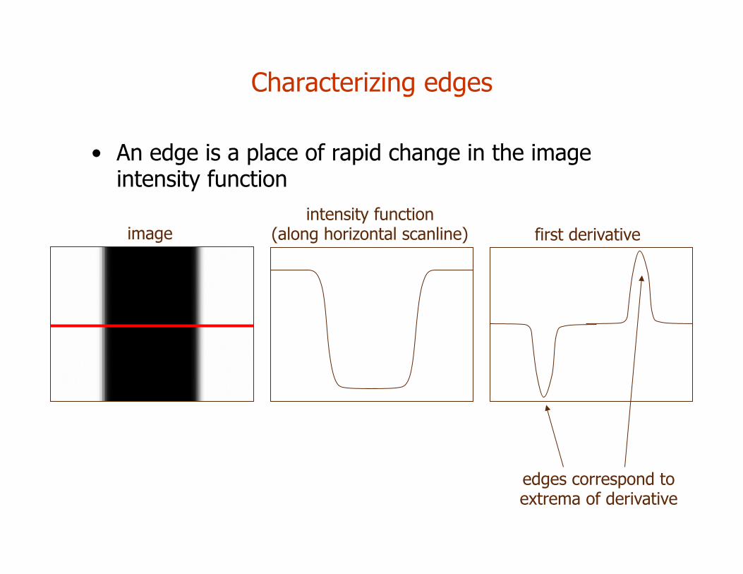
Characterizing edges
• An edge is a place of rapid change in the image intensity function
image intensity function
(along horizontal scanline) first derivative
edges correspond to extrema of derivative
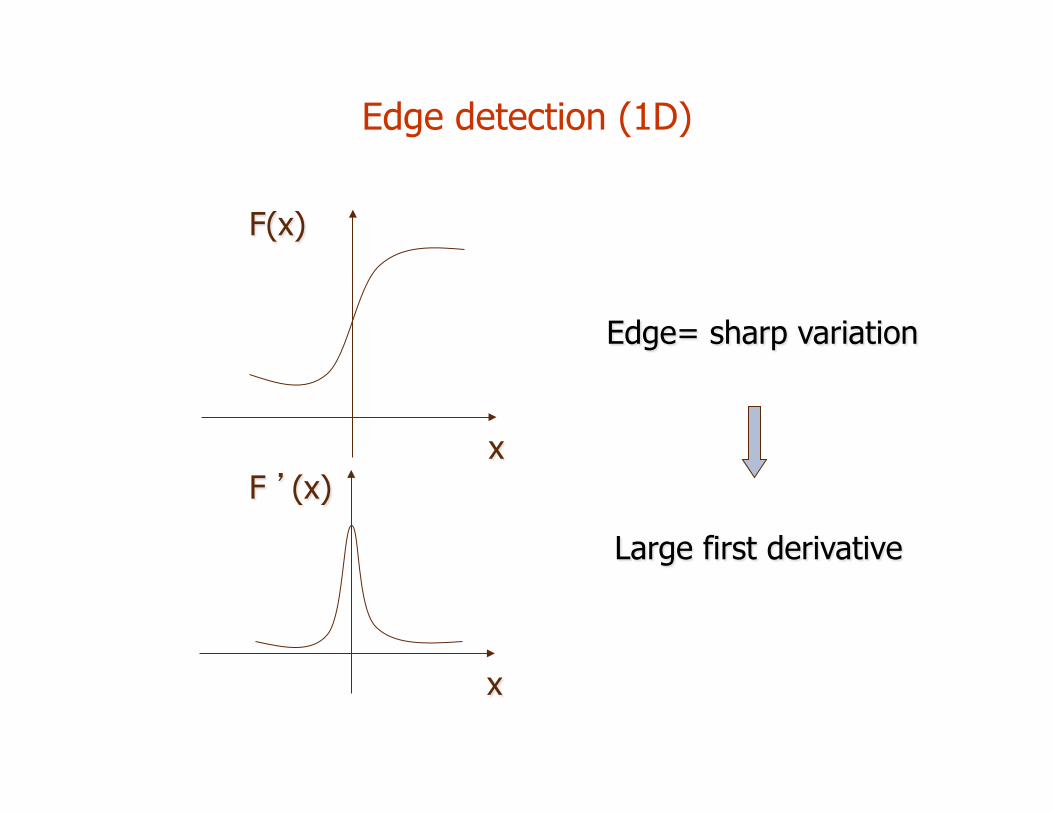
Edge detection (1D)
F(x)
x F ’(x)
x
Edge= sharp variation
Large first derivative
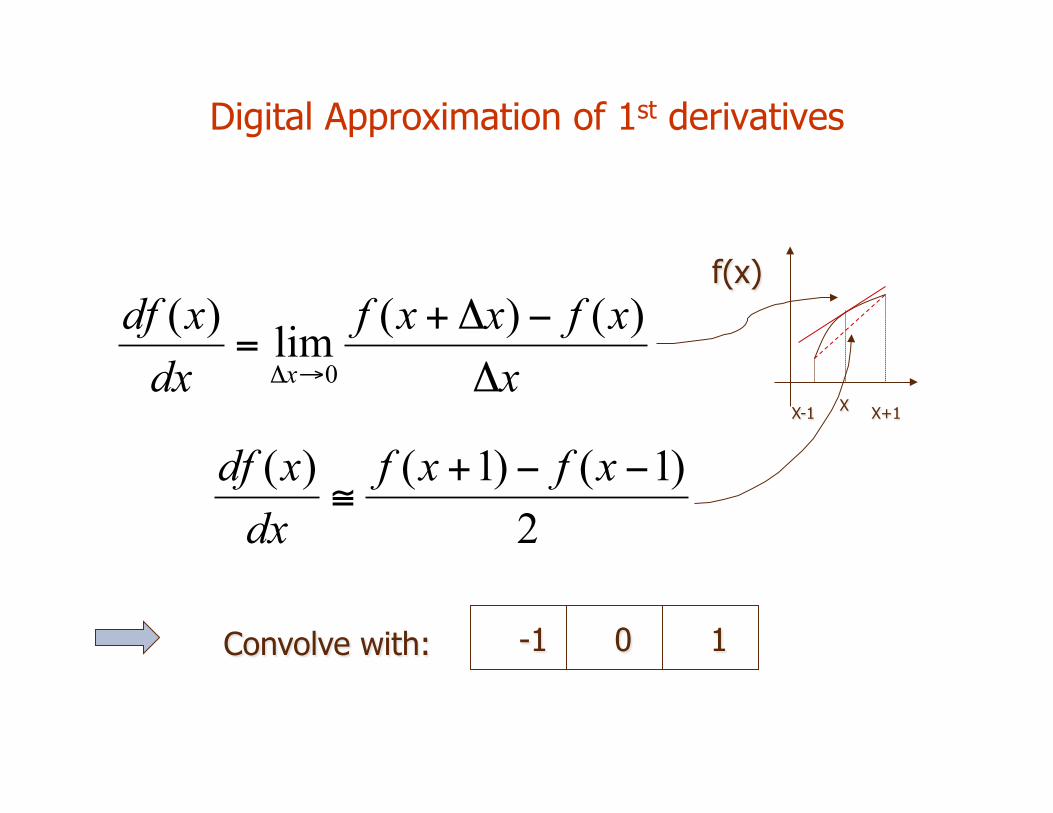
Digital Approximation of 1st derivatives
xxfxxf
dxxdf
x Δ
−Δ+=
→Δ
)()(lim)(0
2)1()1()( −−+
≅xfxf
dxxdf
X
f(x)
X-1 X+1
-1 0 1 Convolve with:
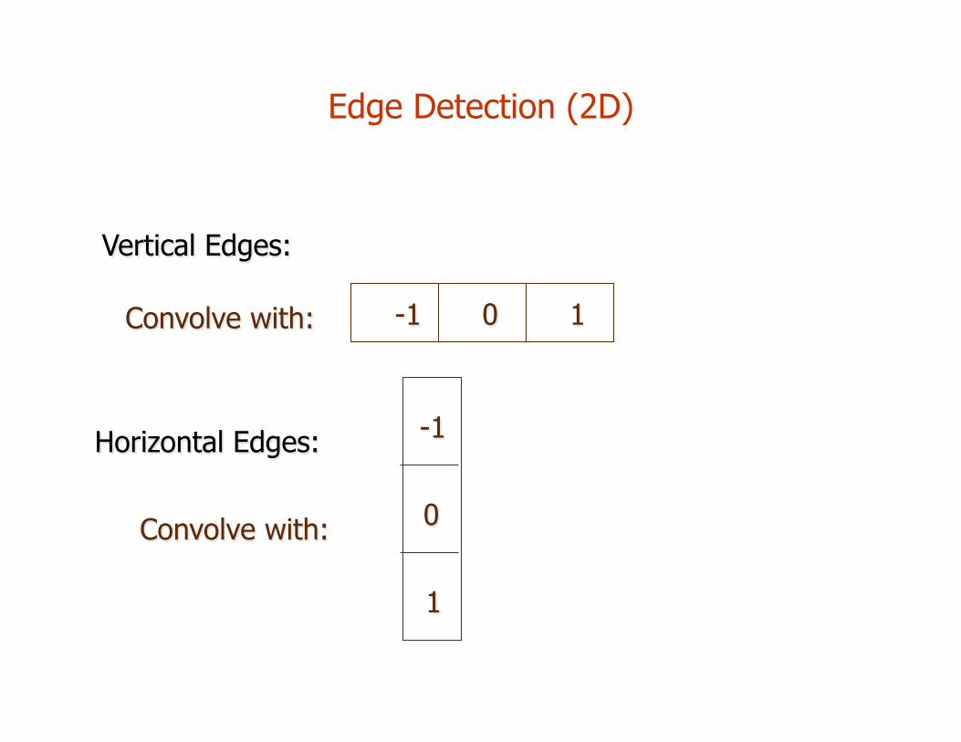
Edge Detection (2D)
-1 0 1 Convolve with:
Vertical Edges:
Horizontal Edges:
Convolve with:
-1
0
1
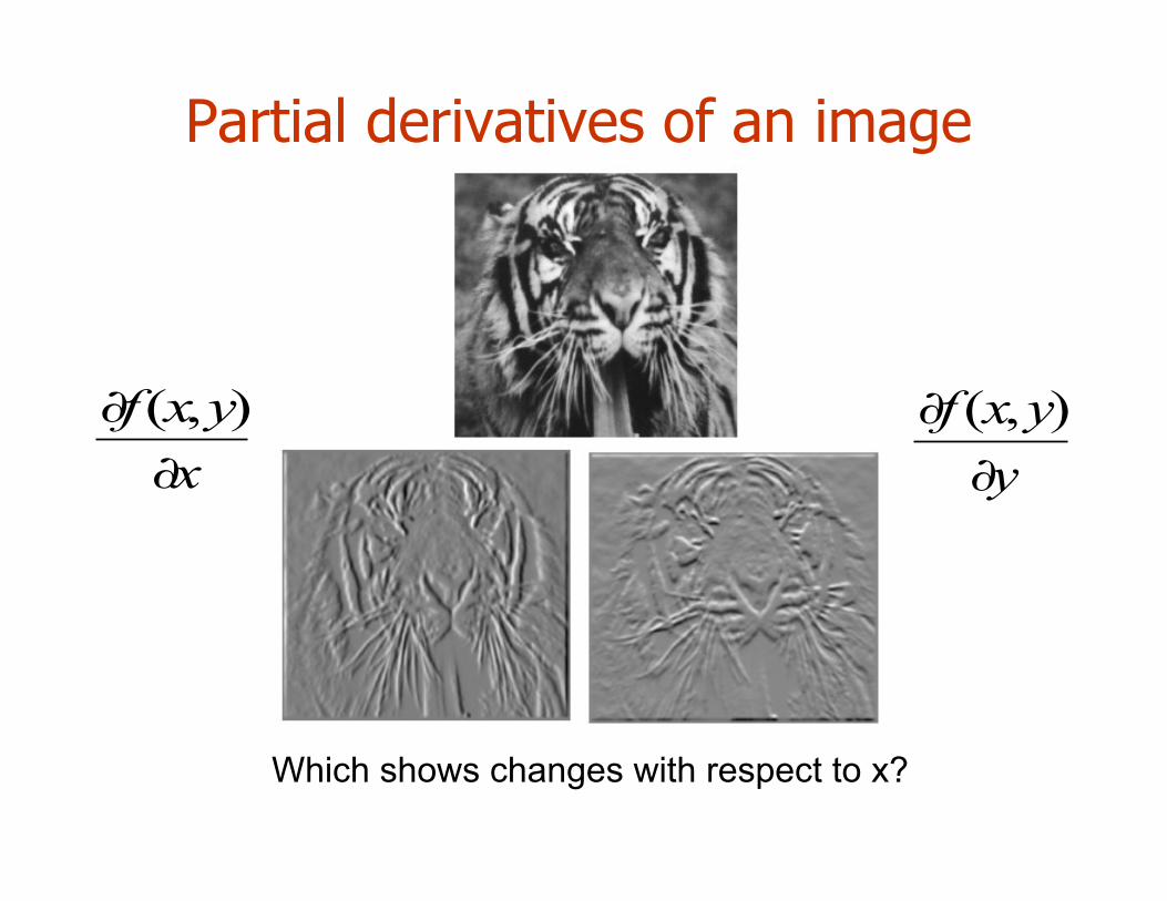
Partial derivatives of an image
Which shows changes with respect to x?
xyxf
∂
∂ ),(yyxf
∂
∂ ),(
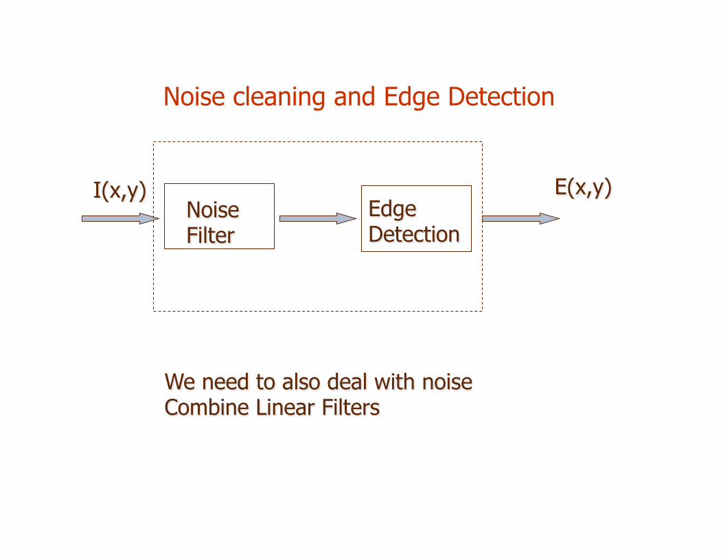
Noise cleaning and Edge Detection
Noise Filter
Edge Detection
I(x,y)
We need to also deal with noise Combine Linear Filters
E(x,y)
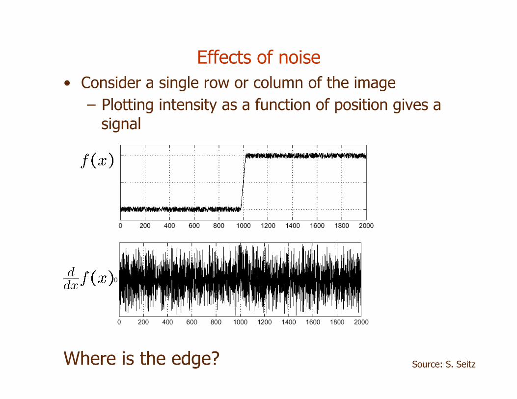
Effects of noise • Consider a single row or column of the image
– Plotting intensity as a function of position gives a signal
Where is the edge? Source: S. Seitz
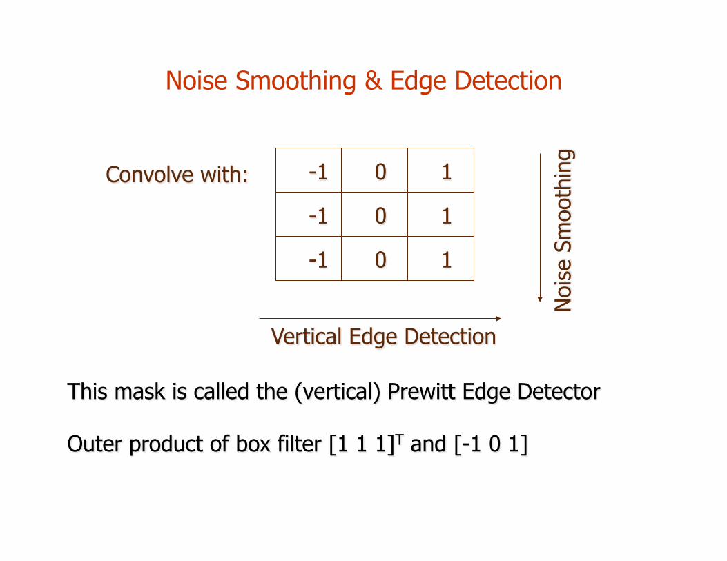
Noise Smoothing & Edge Detection
Convolve with: -1 0 1
-1 0 1
-1 0 1
Vertical Edge Detection
Noi
se S
moo
thin
g
This mask is called the (vertical) Prewitt Edge Detector Outer product of box filter [1 1 1]T and [-1 0 1]
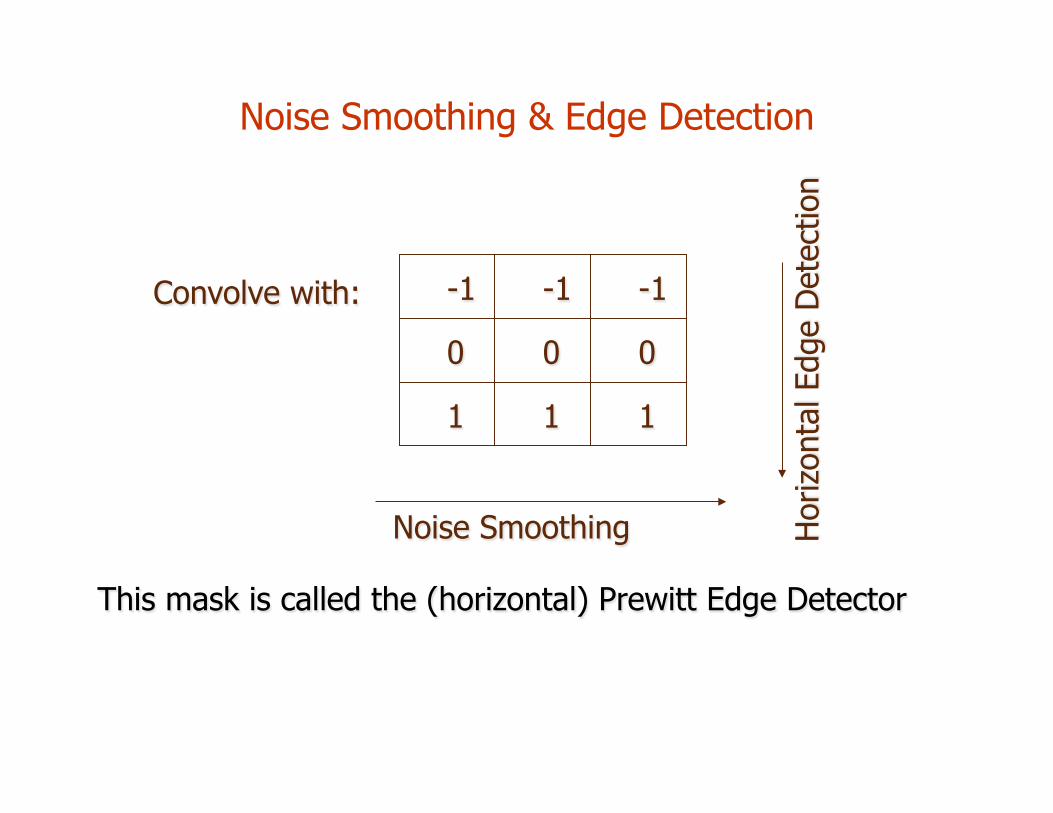
Noise Smoothing & Edge Detection
Convolve with: -1 -1 -1
0 0 0
1 1 1
Noise Smoothing Hor
izon
tal E
dge
Det
ectio
n
This mask is called the (horizontal) Prewitt Edge Detector
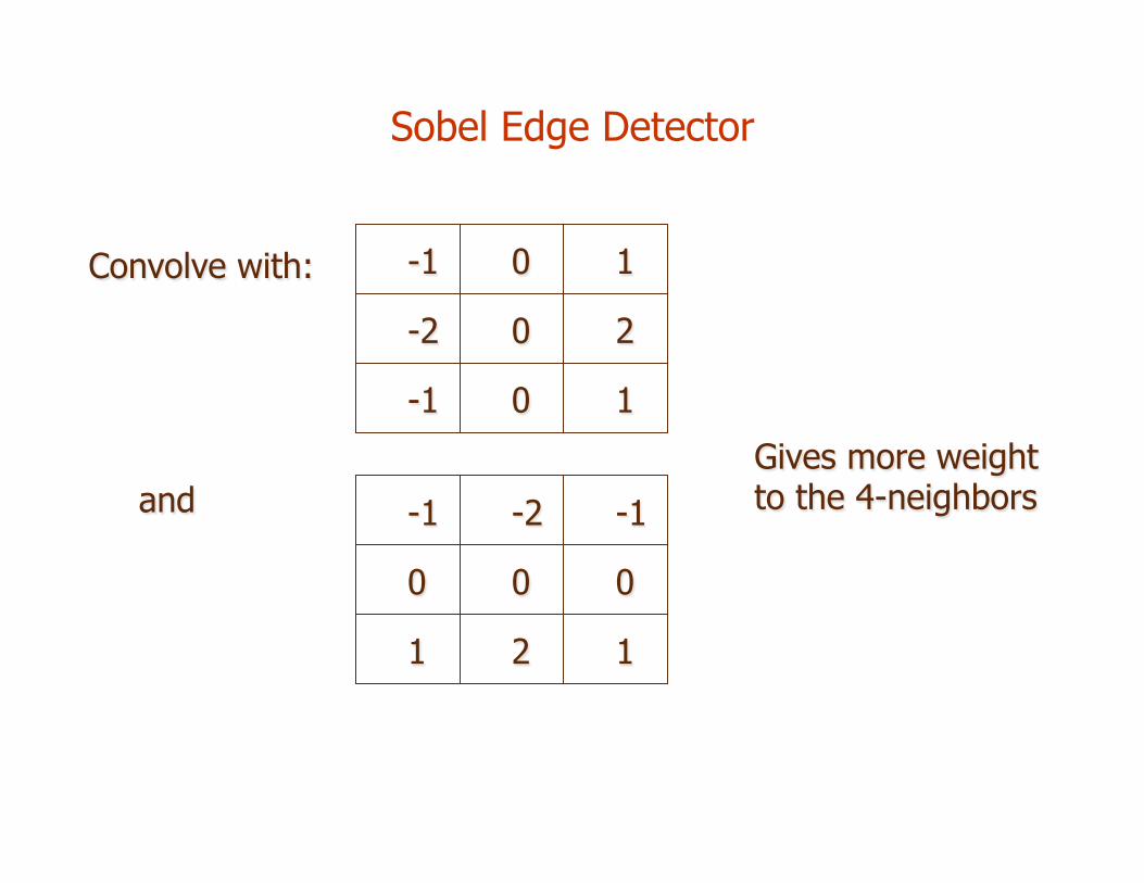
Sobel Edge Detector
Convolve with: -1 0 1
-2 0 2
-1 0 1
and -1 -2 -1
0 0 0
1 2 1
Gives more weight to the 4-neighbors
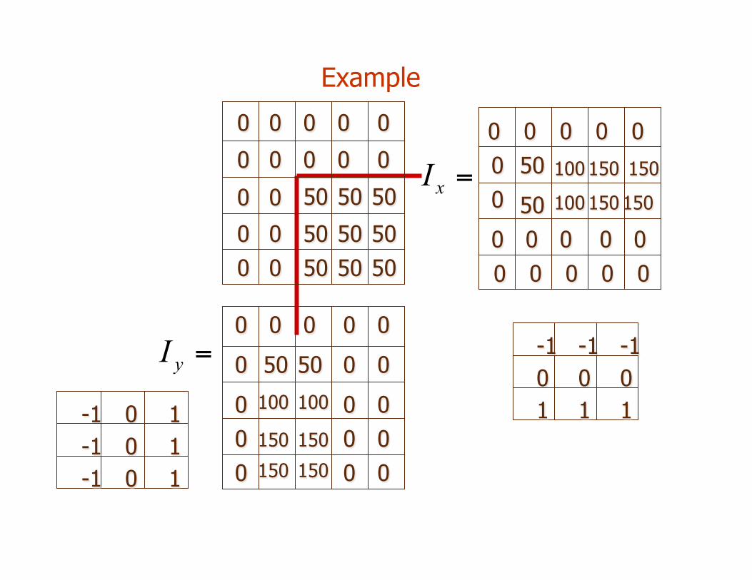
Example
-1 0 1 -1 0 1 -1 0 1
-1 -1 -1 0 0 0 1 1 1
0 0 0 0 0
0 0 0 0 0
0
0 0
0
0 0
50 50 50
50 50 50 50 50 50
50 50 0
100
150 150
0 0
100
0
0 0
0
0 0
0 0 0 0 0
0 0 0 150 150
0 0 0 0 0
0
0 0
0 0 0 0 0 0
50
50 0 0 0
100
100
150
150
150
150 =xI
=yI
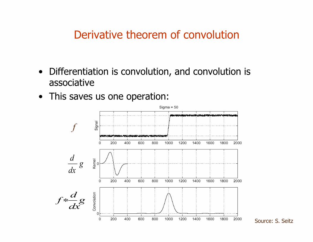
• Differentiation is convolution, and convolution is associative
• This saves us one operation:
Derivative theorem of convolution
gdxdf ∗
f
gdxd
Source: S. Seitz
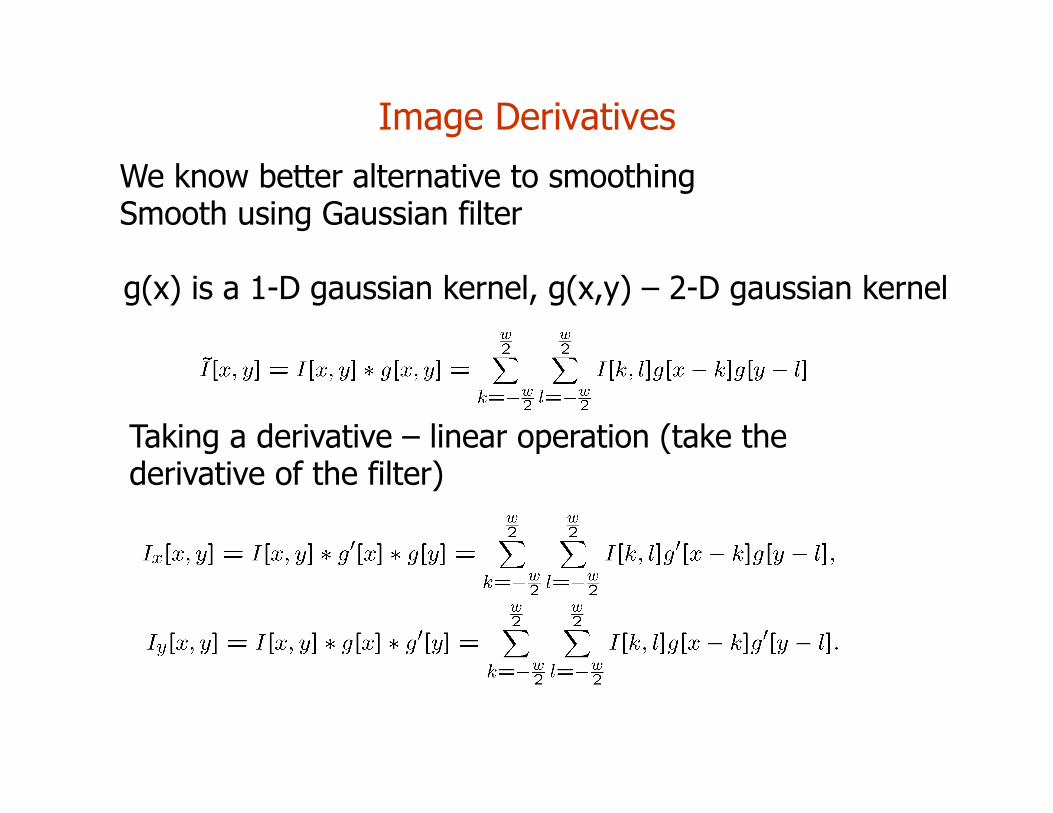
Image Derivatives We know better alternative to smoothing Smooth using Gaussian filter
Taking a derivative – linear operation (take the derivative of the filter)
g(x) is a 1-D gaussian kernel, g(x,y) – 2-D gaussian kernel
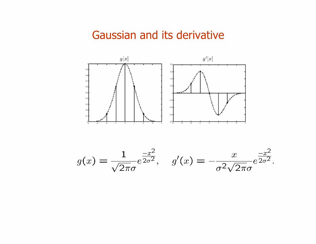
Gaussian and its derivative
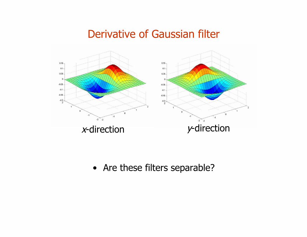
Derivative of Gaussian filter
• Are these filters separable?
x-direction y-direction
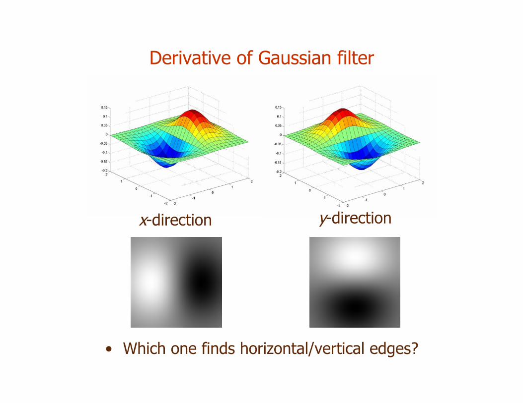
Derivative of Gaussian filter
• Which one finds horizontal/vertical edges?
x-direction y-direction
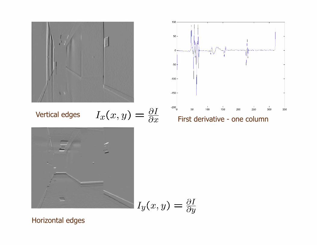
Vertical edges First derivative - one column
Horizontal edges
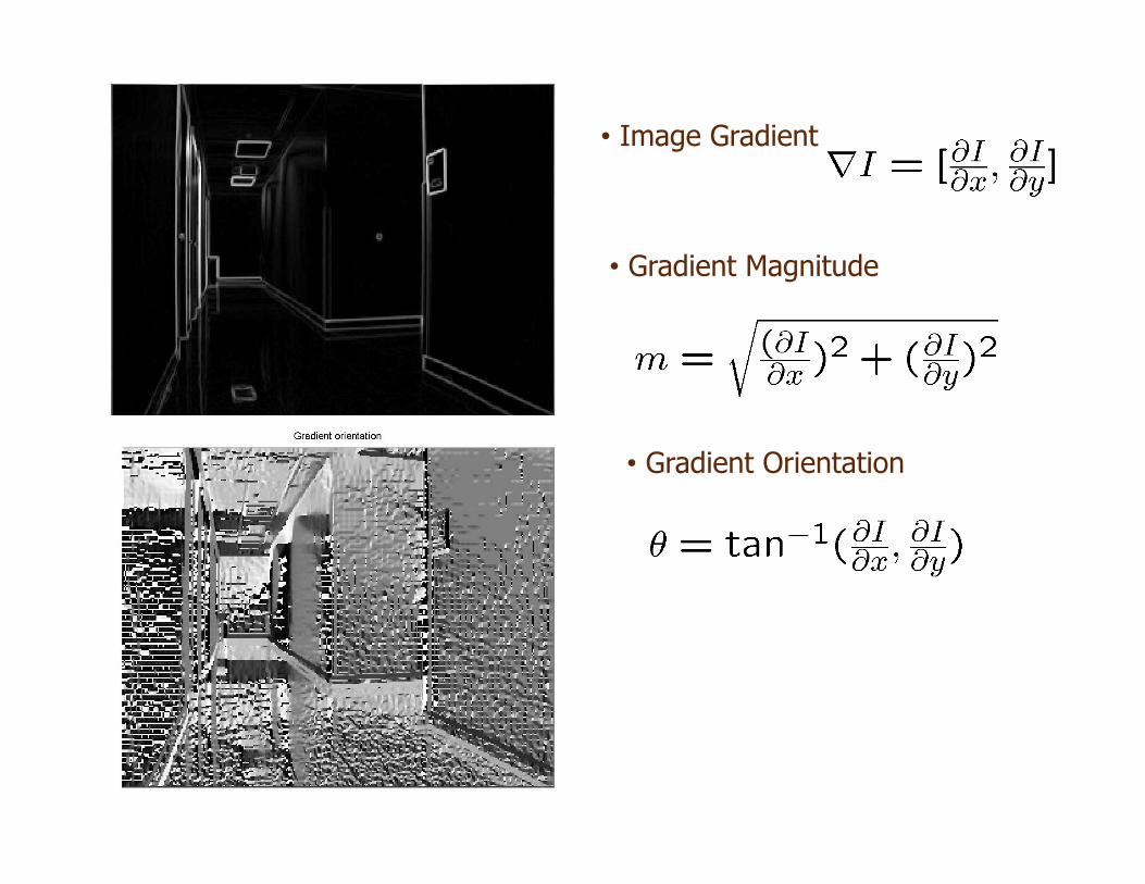
• Image Gradient
• Gradient Magnitude
• Gradient Orientation
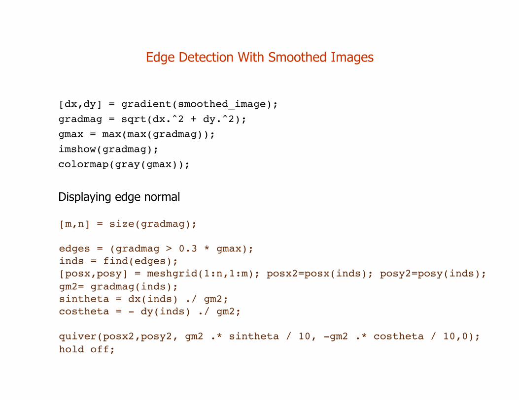
Edge Detection With Smoothed Images
[dx,dy] = gradient(smoothed_image);gradmag = sqrt(dx.^2 + dy.^2);gmax = max(max(gradmag));imshow(gradmag);colormap(gray(gmax));
Displaying edge normal
[m,n] = size(gradmag);
edges = (gradmag > 0.3 * gmax);inds = find(edges);[posx,posy] = meshgrid(1:n,1:m); posx2=posx(inds); posy2=posy(inds);gm2= gradmag(inds);sintheta = dx(inds) ./ gm2;costheta = - dy(inds) ./ gm2;
quiver(posx2,posy2, gm2 .* sintheta / 10, -gm2 .* costheta / 10,0);hold off;
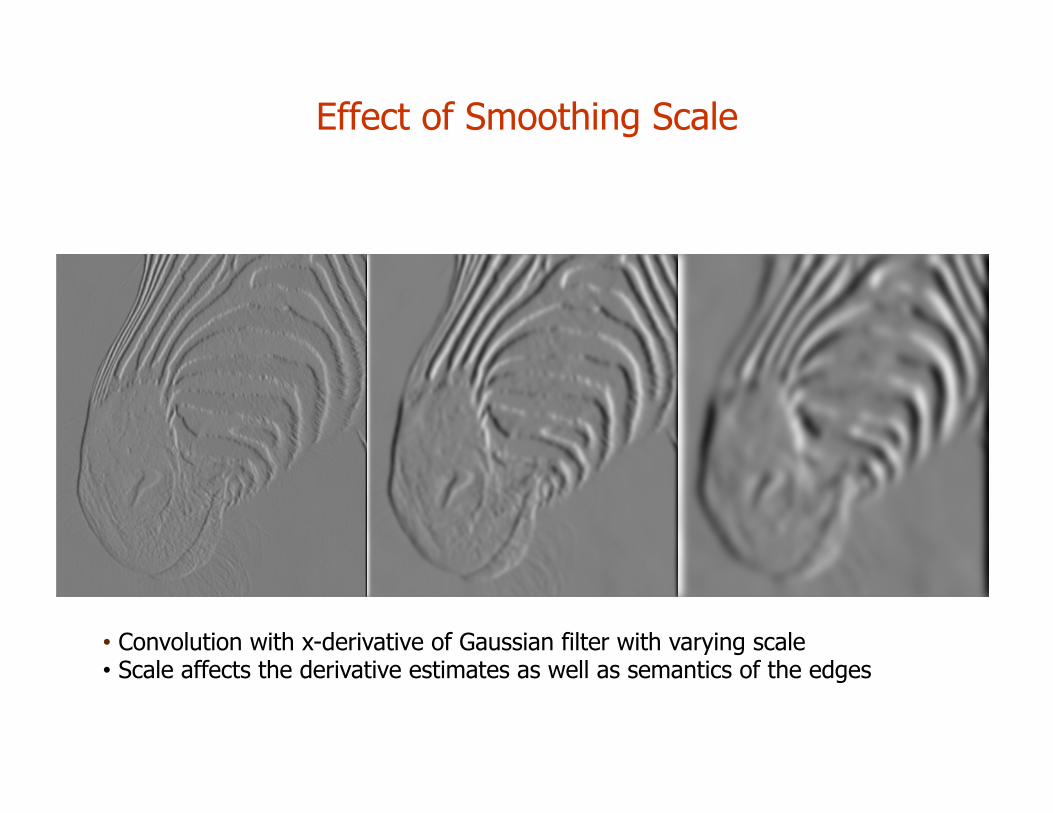
Effect of Smoothing Scale
• Convolution with x-derivative of Gaussian filter with varying scale • Scale affects the derivative estimates as well as semantics of the edges
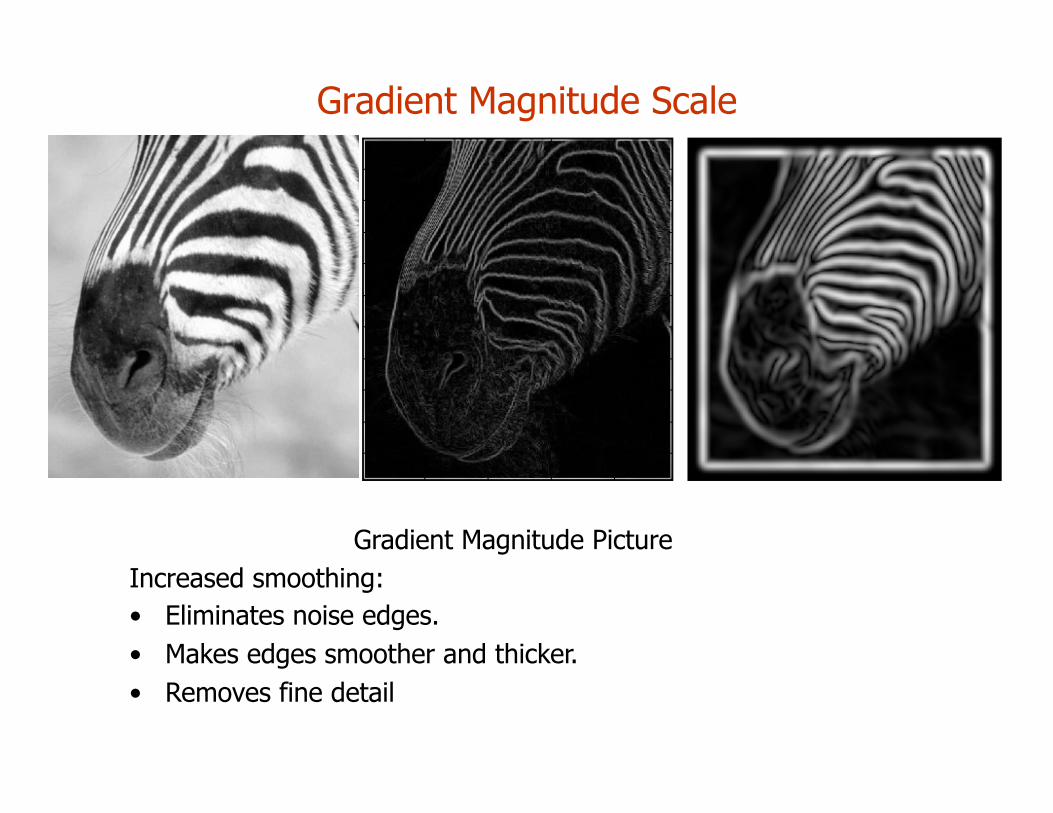
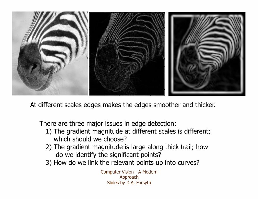
Gradient Magnitude Scale
Gradient Magnitude Picture Increased smoothing: • Eliminates noise edges. • Makes edges smoother and thicker. • Removes fine detail
Computer Vision - A Modern Approach
Slides by D.A. Forsyth
There are three major issues in edge detection: 1) The gradient magnitude at different scales is different; which should we choose? 2) The gradient magnitude is large along thick trail; how do we identify the significant points? 3) How do we link the relevant points up into curves?
At different scales edges makes the edges smoother and thicker.
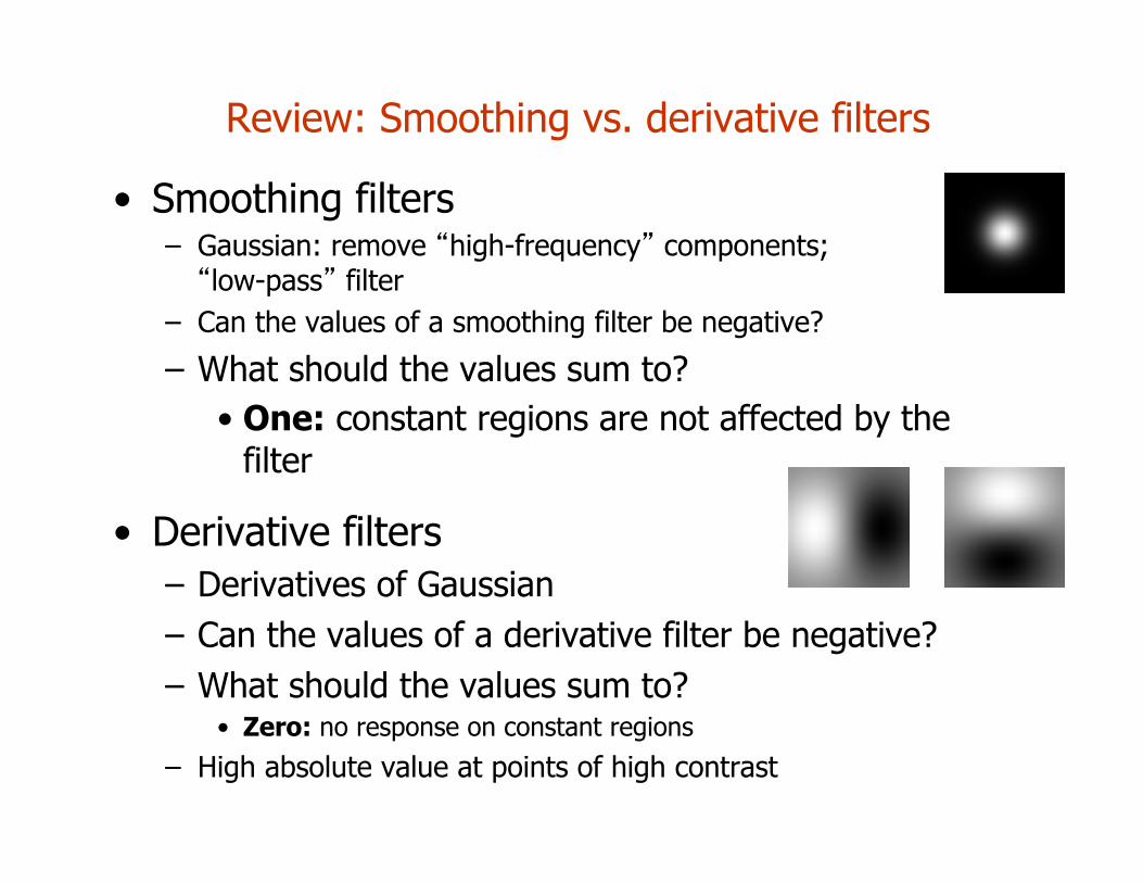
Review: Smoothing vs. derivative filters
• Smoothing filters – Gaussian: remove “high-frequency” components; “low-pass” filter
– Can the values of a smoothing filter be negative?
– What should the values sum to?
• One: constant regions are not affected by the filter
• Derivative filters – Derivatives of Gaussian – Can the values of a derivative filter be negative? – What should the values sum to?
• Zero: no response on constant regions
– High absolute value at points of high contrast
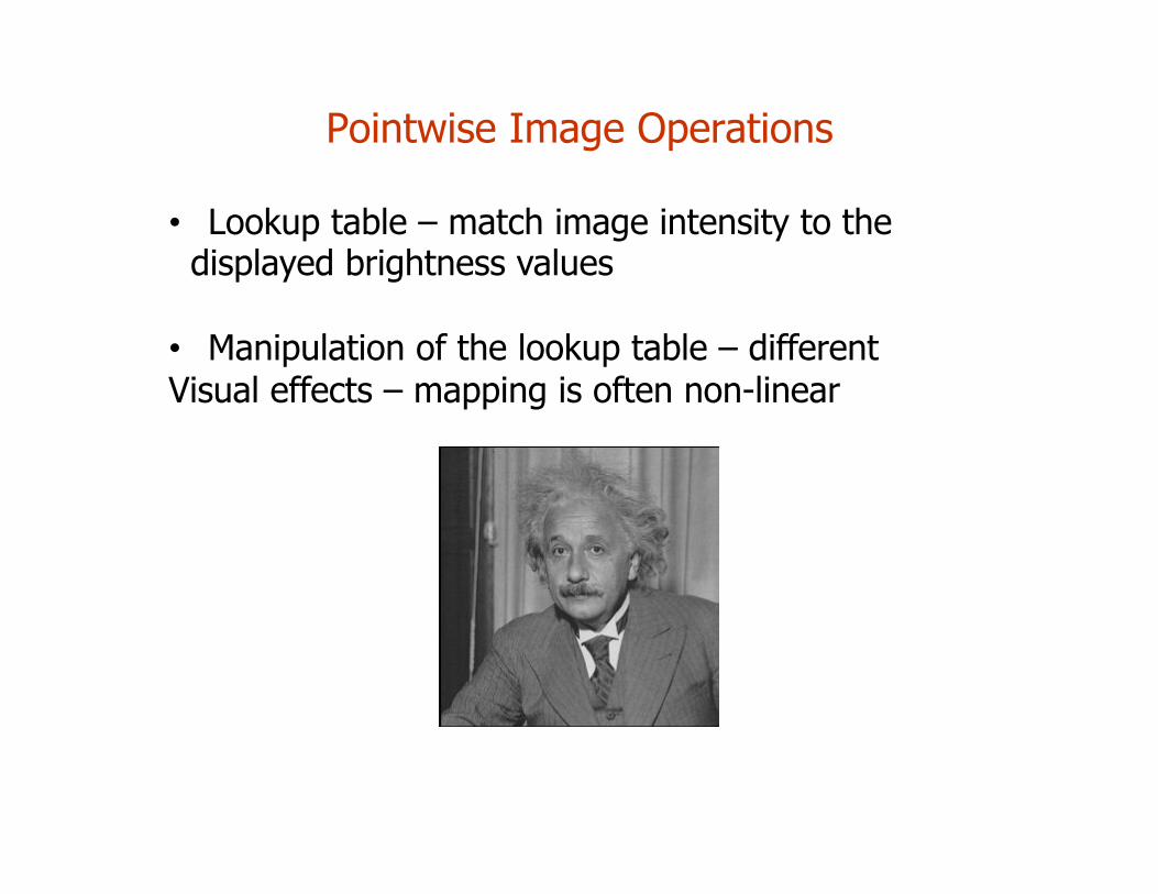
Pointwise Image Operations
• Lookup table – match image intensity to the displayed brightness values • Manipulation of the lookup table – different Visual effects – mapping is often non-linear
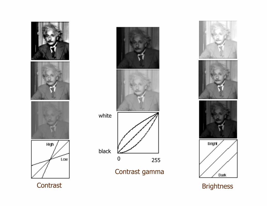
Contrast gamma
Contrast Brightness
0 255
white
black
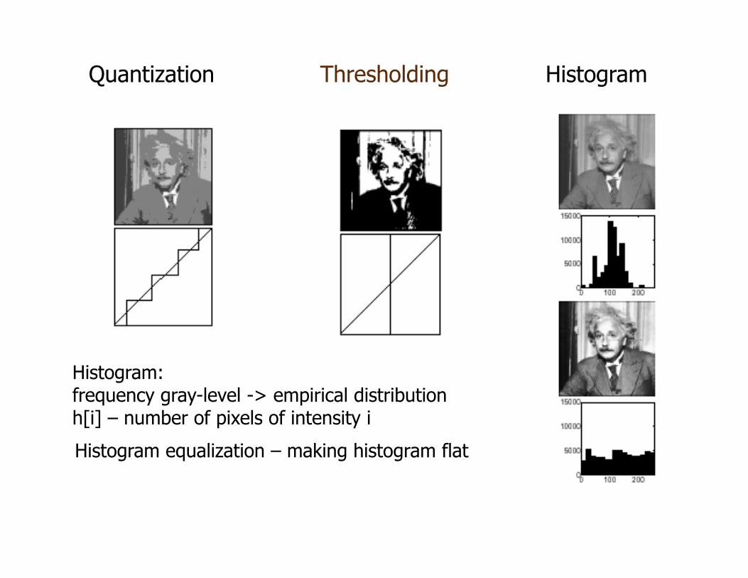
Quantization Thresholding Histogram
Histogram equalization – making histogram flat
Histogram: frequency gray-level -> empirical distribution h[i] – number of pixels of intensity i