Embed Size (px)
Citation preview

1G52IVG, School of Computer Science, University of Nottingham
Image Compression
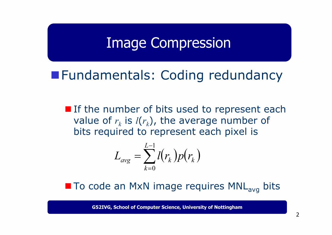
Fundamentals: Coding redundancy
The gray level histogram of an image can reveal a great deal of information about the image
That probability (frequency) of occurrence of gray level rk is p(rk),
( ) 1,...,2,0 −== Lknnrp k
k
2G52IVG, School of Computer Science, University of Nottingham
Image Compression
Fundamentals: Coding redundancy
If the number of bits used to represent each value of rk is l(rk), the average number of bits required to represent each pixel is
To code an MxN image requires MNLavg bits
( ) ( )∑−
=
=1
0
L
kkkavg rprlL

3G52IVG, School of Computer Science, University of Nottingham
Image Compression
Fundamentals: Coding redundancy
some pixel values more common than others

4G52IVG, School of Computer Science, University of Nottingham
Image Compression
Fundamentals: Coding redundancy
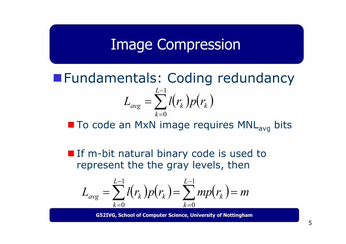
To code an MxN image requires MNLavg bits
If m-bit natural binary code is used to represent the the gray levels, then
( ) ( )∑−
=
=1
0
L
kkkavg rprlL
( ) ( ) ( ) mrmprprlLL
kk
L
kkkavg === ∑∑
−
=
−
=
1
0
1
0
5G52IVG, School of Computer Science, University of Nottingham
Image Compression
Fundamentals: Coding redundancy
To code an MxN image requires MNLavg bits
If m-bit natural binary code is used to represent the the gray levels, then
( ) ( )∑−
=
=1
0
L
kkkavg rprlL
( ) ( ) ( ) mrmprprlLL
kk
L
kkkavg === ∑∑
−
=
−
=
1
0
1
0

6G52IVG, School of Computer Science, University of Nottingham
Image Compression
Fundamentals: Coding redundancyVariable length Coding: assign fewer bits to the more probable gray levels than to less probable ones can achieve data compression

7G52IVG, School of Computer Science, University of Nottingham
Image Compression
Fundamentals: Interpixel (spatial) redundancy
neighboring pixels have similar values
Binary imagesGray scale image (later)
8G52IVG, School of Computer Science, University of Nottingham
Image Compression
Fundamentals: Interpixel (spatial) redundancy: Binary images
Run-length codingMapping the pixels along each scan line into a sequence of pairs (g1, r1), (g2, r2), …, Where gi is the ith gray level, ri is the run length of ith run
9G52IVG, School of Computer Science, University of Nottingham
Image Compression
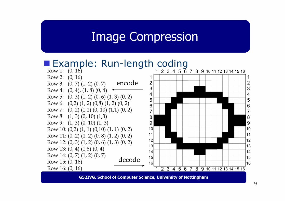
Example: Run-length coding
decode
1 2 3 4 5 6 7 8 9 10 11 12 13 14 15 16123456
111213141516
789
123456789
1 2 3 4 5 6 7 8 9 11 12 13 14 15 16
111213141516
10
10 10
Row 1: (0, 16)Row 2: (0, 16)Row 3: (0, 7) (1, 2) (0, 7)Row 4: (0, 4), (1, 8) (0, 4)Row 5: (0, 3) (1, 2) (0, 6) (1, 3) (0, 2)Row 6: (0,2) (1, 2) (0,8) (1, 2) (0, 2)Row 7: (0, 2) (1,1) (0, 10) (1,1) (0, 2)Row 8: (1, 3) (0, 10) (1,3)Row 9: (1, 3) (0, 10) (1, 3)Row 10: (0,2) (1, 1) (0,10) (1, 1) (0, 2)Row 11: (0, 2) (1, 2) (0, 8) (1, 2) (0, 2)Row 12: (0, 3) (1, 2) (0, 6) (1, 3) (0, 2)Row 13: (0, 4) (1,8) (0, 4)Row 14: (0, 7) (1, 2) (0, 7)Row 15: (0, 16)Row 16: (0, 16)
encode

10G52IVG, School of Computer Science, University of Nottingham
Image Compression
Fundamentals: Psychovisualredundancy
some color differences are imperceptible

11G52IVG, School of Computer Science, University of Nottingham
Image Compression
Fidelity criteria
Root mean square error (erms) and signal to noise ratio (SNR): Let f(x,y) be the input image, f’(x,y) be reconstructed input image from compressed bit stream, then
( ) ( )( )( )( )
( ) ( )( )∑∑
∑∑∑∑ −
=
−
=
−
=
−
=−
=
−
= −=
−= 1
0
1
0
2
1
0
1
0
22/1
1
0
1
0
2
,,'
,',,'1
M
x
N
y
M
x
N
yM
x
N
yrms
yxfyxf
yxfSNRyxfyxf
MNe
12G52IVG, School of Computer Science, University of Nottingham
Image Compression
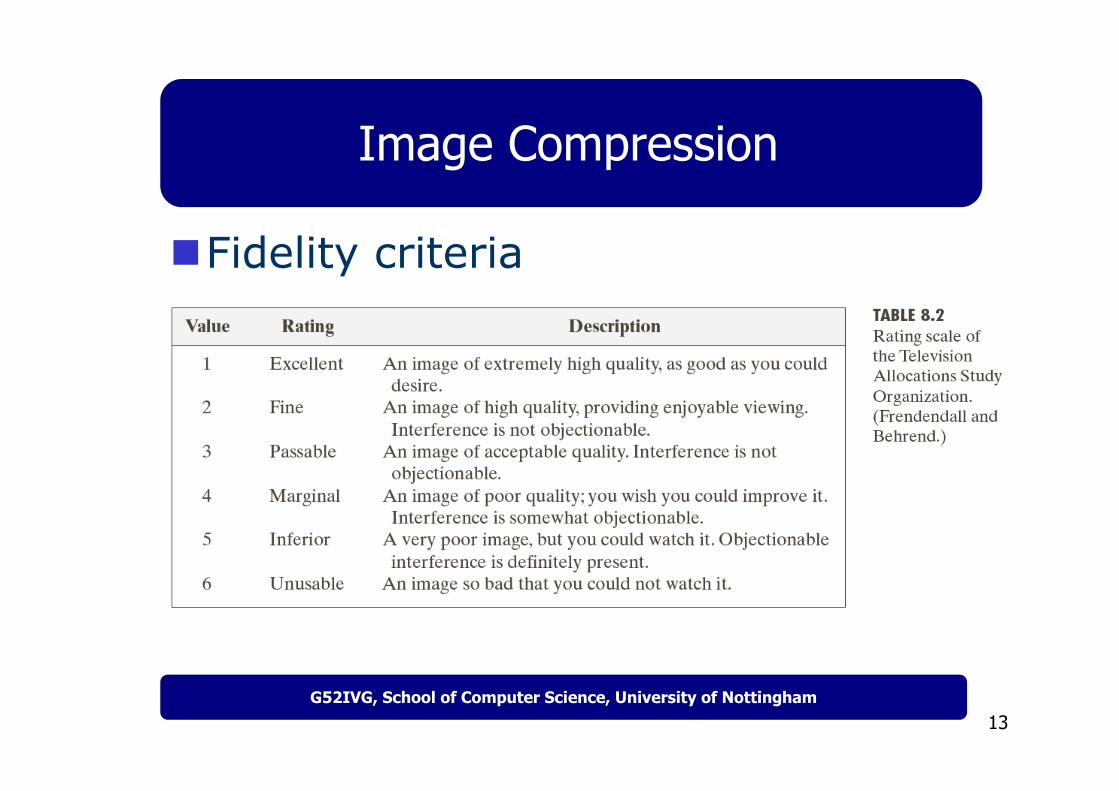
Fidelity criteria
erms and SNR are convenient objective measuresMost decompressed images are view by human beingsSubjective evaluation of compressed image quality by human observers are often more appropriate
13G52IVG, School of Computer Science, University of Nottingham
Image Compression
Fidelity criteria

14G52IVG, School of Computer Science, University of Nottingham
Image Compression
Image compression models
15G52IVG, School of Computer Science, University of Nottingham
Image Compression
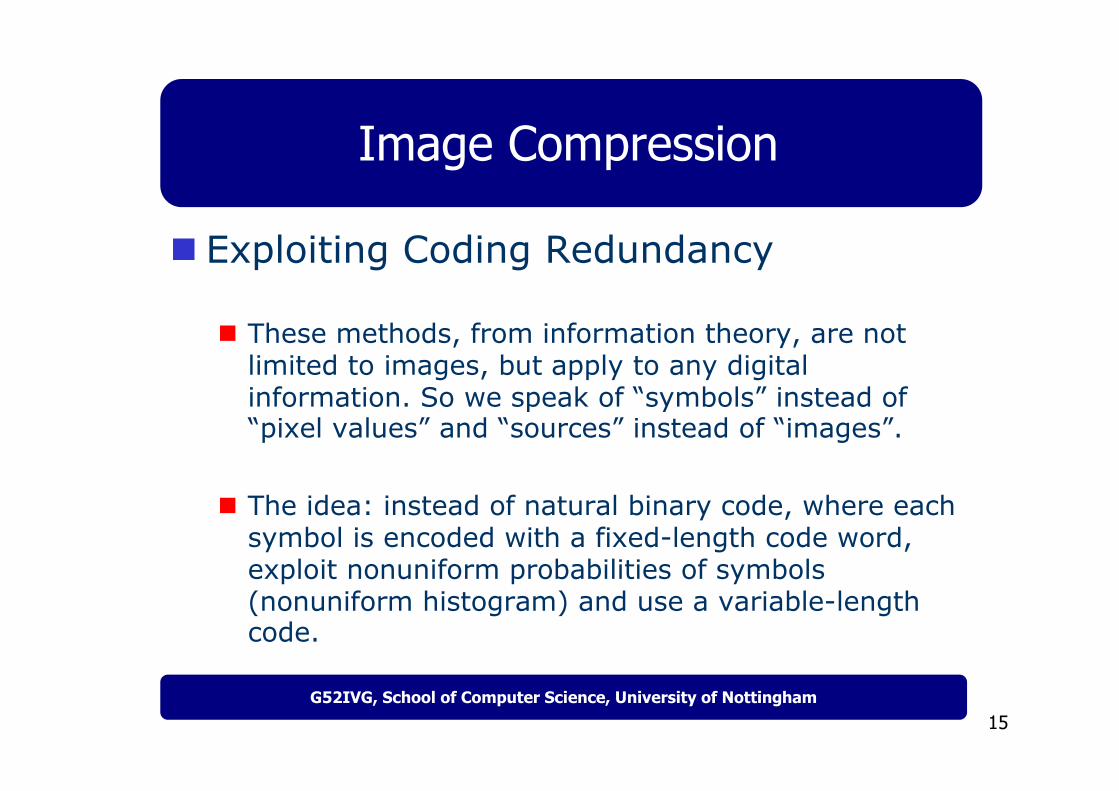
Exploiting Coding Redundancy
These methods, from information theory, are not limited to images, but apply to any digital information. So we speak of “symbols” instead of “pixel values” and “sources” instead of “images”.
The idea: instead of natural binary code, where each symbol is encoded with a fixed-length code word, exploit nonuniform probabilities of symbols (nonuniform histogram) and use a variable-length code.

16G52IVG, School of Computer Science, University of Nottingham
Image Compression
Exploiting Coding Redundancy
Entropy
is a measure of the information content of a source.
If source is an independent random variable then you can’t compress to fewer than H bits per symbol.
Assign the more frequent symbols short bit strings and the less frequent symbols longer bit strings. Best compression when redundancy is high (entropy is low, histogram is highly skewed).
∑−
=
−=1
02 )(log)(
L
kkk rprpH

17G52IVG, School of Computer Science, University of Nottingham
Image Compression
Exploiting Coding Redundancy
Two common methods
Huffman coding and,LZW coding
18G52IVG, School of Computer Science, University of Nottingham
Image Compression
Exploiting Coding Redundancy
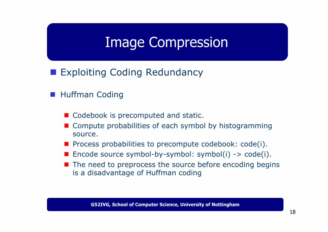
Huffman Coding
Codebook is precomputed and static.Compute probabilities of each symbol by histogrammingsource.Process probabilities to precompute codebook: code(i).Encode source symbol-by-symbol: symbol(i) -> code(i).The need to preprocess the source before encoding begins is a disadvantage of Huffman coding

19G52IVG, School of Computer Science, University of Nottingham
Image Compression
Exploiting Coding Redundancy
Huffman Coding

20G52IVG, School of Computer Science, University of Nottingham
Image Compression
Exploiting Coding Redundancy
Huffman Coding
21G52IVG, School of Computer Science, University of Nottingham
Image Compression
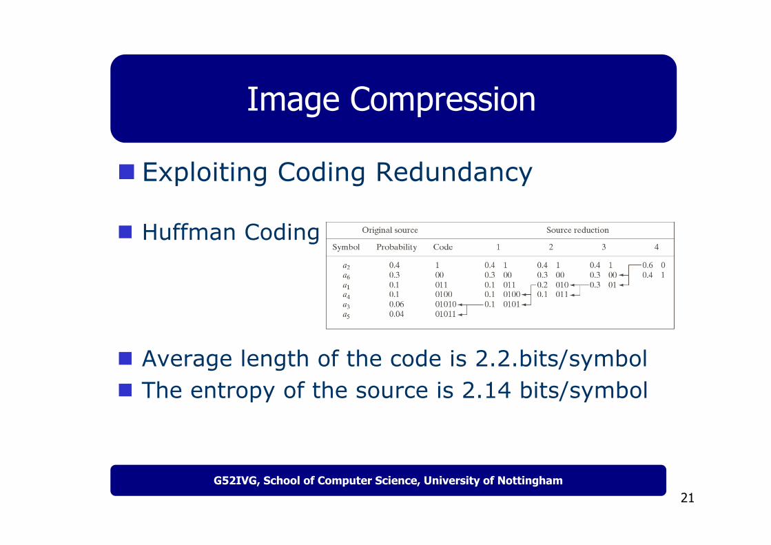
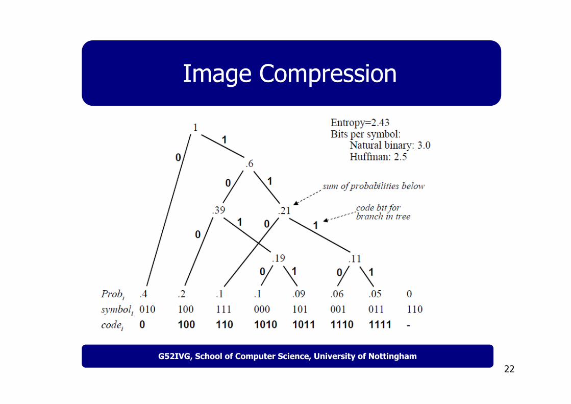
Exploiting Coding Redundancy
Huffman Coding
Average length of the code is 2.2.bits/symbolThe entropy of the source is 2.14 bits/symbol
22G52IVG, School of Computer Science, University of Nottingham
Image Compression
Exploiting Coding Redundancy
Huffman Coding
23G52IVG, School of Computer Science, University of Nottingham
Image Compression
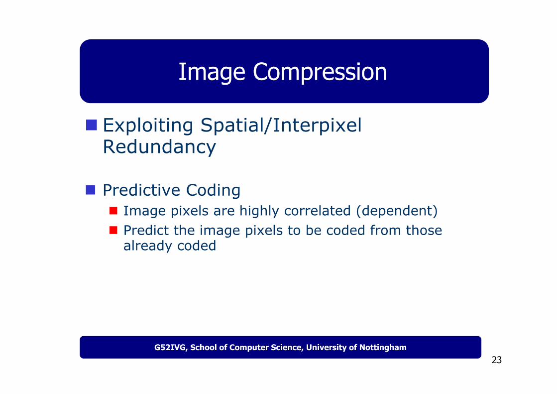
Exploiting Spatial/InterpixelRedundancy
Predictive CodingImage pixels are highly correlated (dependent)Predict the image pixels to be coded from those already coded
24G52IVG, School of Computer Science, University of Nottingham
Image Compression
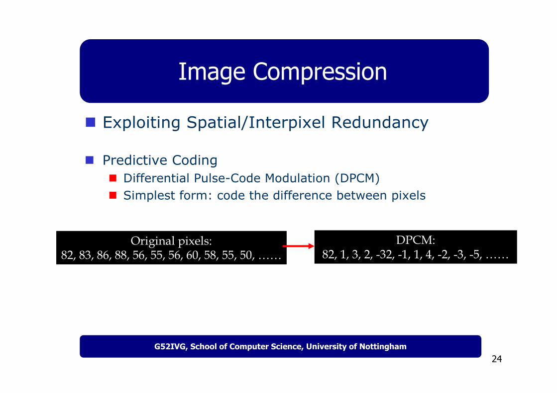
Exploiting Spatial/Interpixel Redundancy
Predictive CodingDifferential Pulse-Code Modulation (DPCM)Simplest form: code the difference between pixels
Original pixels:82, 83, 86, 88, 56, 55, 56, 60, 58, 55, 50, ……
DPCM:82, 1, 3, 2, -32, -1, 1, 4, -2, -3, -5, ……
25G52IVG, School of Computer Science, University of Nottingham
Image Compression
Exploiting Spatial/Interpixel Redundancy
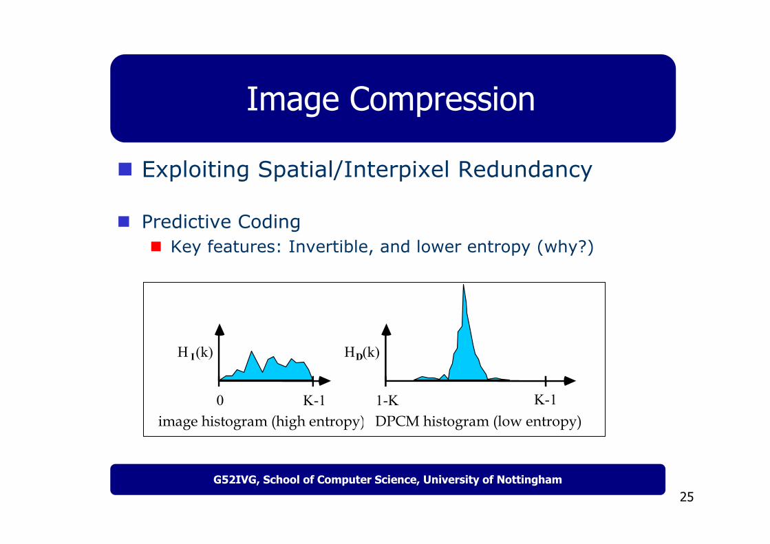
Predictive CodingKey features: Invertible, and lower entropy (why?)
H I(k) HD(k)
high entropy image reduced entropy imageK-10 K-11-K
image histogram (high entropy) DPCM histogram (low entropy)

26G52IVG, School of Computer Science, University of Nottingham
Image Compression
Exploiting Spatial/Interpixel Redundancy
Higher Order (Pattern) PredictionUse both 1D and 2D patterns for prediction
1D Causal:
1D Non-causal:
2D Causal:
2D Non-Causal:

27G52IVG, School of Computer Science, University of Nottingham
Image Compression
Exploiting Spatial/Interpixel Redundancy
2D Causal:

28G52IVG, School of Computer Science, University of Nottingham
Image Compression
Quantization
Quantization: Widely Used in Lossy CompressionRepresent certain image components with fewer bits (compression)With unavoidable distortions (lossy)
Quantizer DesignFind the best tradeoff between
maximal compression minimal distortion
29G52IVG, School of Computer Science, University of Nottingham
Image Compression
Quantization
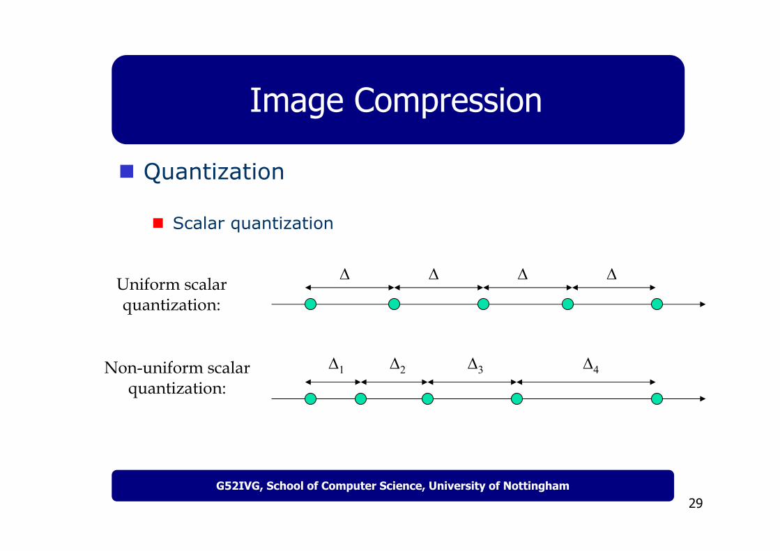
Scalar quantization
24 408 ... 248
∆ ∆∆ ∆
∆2∆1 ∆3 ∆4
Uniform scalar quantization:
Non-uniform scalar quantization:
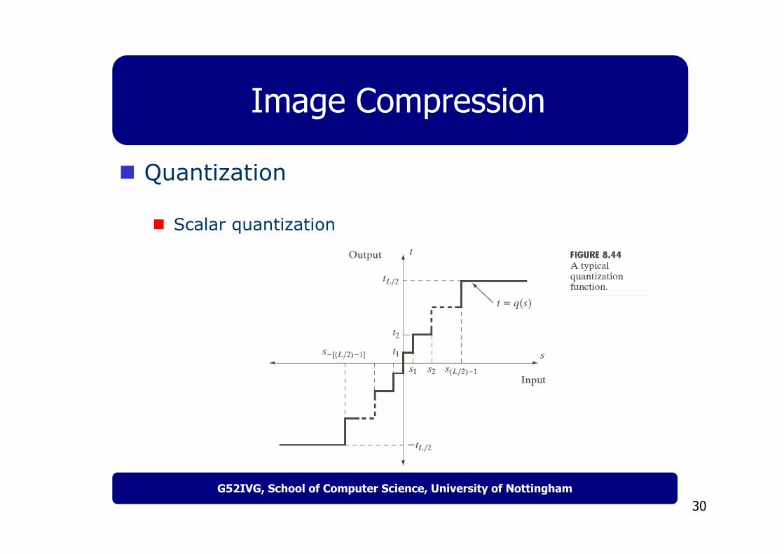
30G52IVG, School of Computer Science, University of Nottingham
Image Compression
Quantization
Scalar quantization
31G52IVG, School of Computer Science, University of Nottingham
Image Compression
Quantization
Vector quantization and palletized images (gif format)

32G52IVG, School of Computer Science, University of Nottingham
Image Compression
Palletized color image (gif)A true colour image – 24bits/pixel, R – 8 bits, G – 8 bits, B – 8 bits
A gif image - 8bits/pixel
1677216 possible colours
256 possible colours

33G52IVG, School of Computer Science, University of Nottingham
Image Compression
Palletized color image (gif)A true colour image – 24bits/pixel, R – 8 bits, G – 8 bits, B – 8 bits
A gif image - 8bits/pixel
1677216 possible colours
256 possible colours
Exploits psychovisualredundancy
34G52IVG, School of Computer Science, University of Nottingham
Image Compression
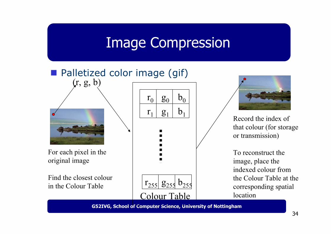
Palletized color image (gif)
r0 g0 b0
r1 g1 b1
r255 g255 b255
(r, g, b)
Colour Table
For each pixel in the original image
Find the closest colour in the Colour Table
Record the index of that colour (for storage or transmission)
To reconstruct the image, place the indexed colour from the Colour Table at the corresponding spatial location

35G52IVG, School of Computer Science, University of Nottingham
Image Compression
Palletized color image (gif)
r0 g0 b0
r1 g1 b1
r255 g255 b255
(r, g, b)
Colour Table
For each pixel in the original image
Find the closest colour in the Colour Table
Record the index of that colour (for storage or transmission)
To reconstruct the image, place the indexed colour from the Colour Table at the corresponding spatial location
How to choose the colours in the table/pallet?
36G52IVG, School of Computer Science, University of Nottingham
Image Compression
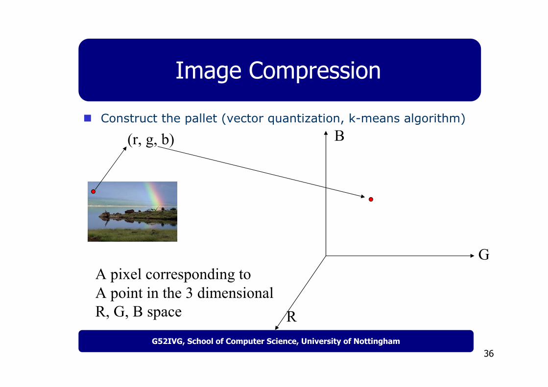
Construct the pallet (vector quantization, k-means algorithm)
(r, g, b)
R
G
B
A pixel corresponding toA point in the 3 dimensional R, G, B space
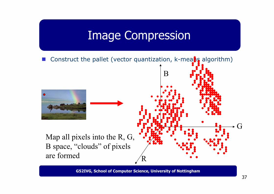
37G52IVG, School of Computer Science, University of Nottingham
Image Compression
Construct the pallet (vector quantization, k-means algorithm)
R
G
B
Map all pixels into the R, G, B space, “clouds” of pixels are formed

38G52IVG, School of Computer Science, University of Nottingham
Image Compression
Construct the pallet (vector quantization, k-means algorithm)
R
G
BGroup pixels that are close to each other, and replace them by one single colour
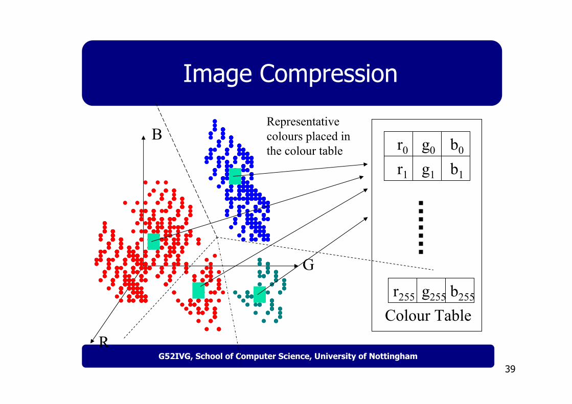
39G52IVG, School of Computer Science, University of Nottingham
Image Compression
R
G
B r0 g0 b0
r1 g1 b1
r255 g255 b255
Colour Table
Representative colours placed in the colour table

40G52IVG, School of Computer Science, University of Nottingham
Image Compression
Discrete Cosine Transform (DCT)2D-DCT
Inverse 2D-DCT
∑∑−
=
−
=
+
+
=1
0
1
02 2
)12(cos2
)12(cos),()()(4),(N
m
N
n Nvn
Numnmx
NvCuCvuX ππ
∑∑−
=
−
=
+
+
=1
0
1
0 2)12(cos
2)12(cos),()()(),(
N
u
N
v Nvn
NumvuXvCuCnmx ππ
−=
==1,,11
02
1)(
Nu
uuCL
where
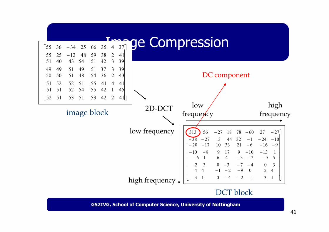
41G52IVG, School of Computer Science, University of Nottingham
Image Compression
−−
412451
42534255
51535452
51525151
414432
41553654
51524851
52515050
393393
37514251
49515443
49494051
412374
38593566
48122534
25553655
−−−
−−−
−−−−−
−−
−−−
−−
−−−−
−−−
−−−
−−
1342
1209
4021
1344
3055
4773
3046
3216
113916
109621
1793310
8101720
10242727
1326078
44131827
273856313
2D-DCTimage block
DCT block
low frequency
high frequency
low frequency
high frequency
DC component

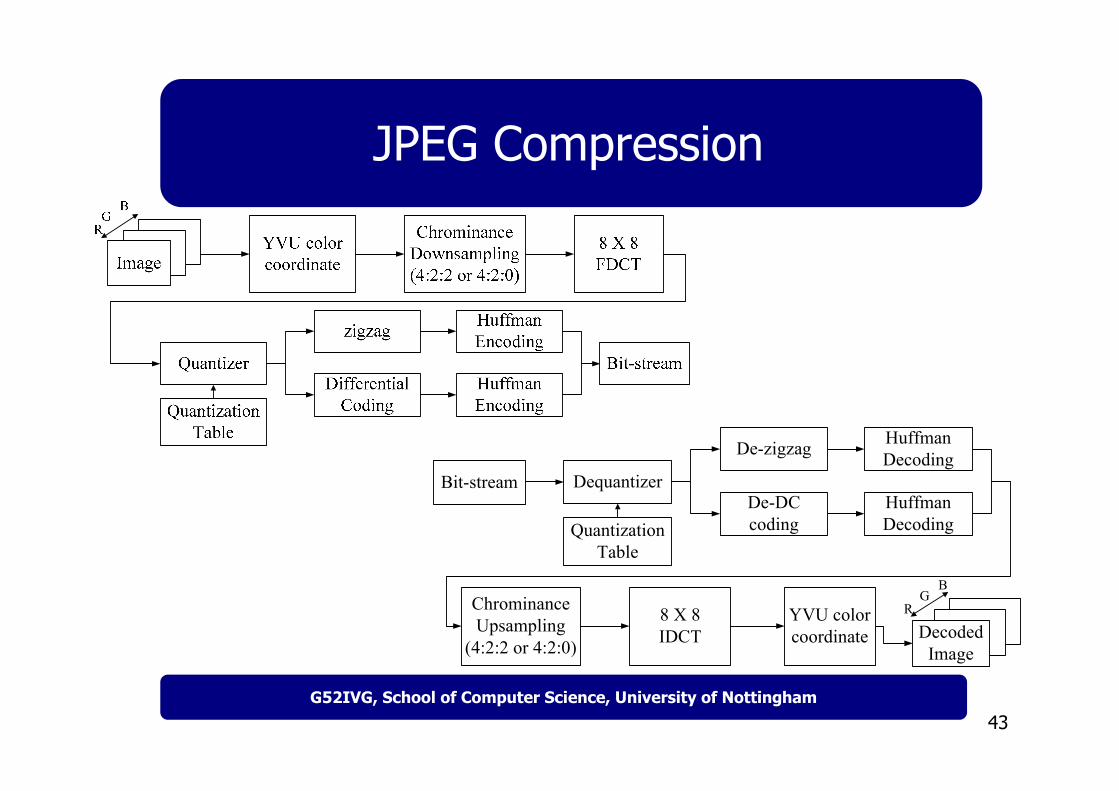
42G52IVG, School of Computer Science, University of Nottingham
JPEG Compression
169130173129
170181170183
179181182180
179180179179
169132171130
169183164182
179180176179
180179178178
167131167131
165179170179
177179182171
177177168179
169130165132
166187163194
17611615394
153183160183
−−
412451
42534255
51535452
51525151
414432
41553654
51524851
52515050
393393
37514251
49515443
49494051
412374
38593566
48122534
25553655
- 128
−−−
−−−
−−−−−
−−
−−−
−−
−−−−
−−−
−−−
−−
1342
1209
4021
1344
3055
4773
3046
3216
113916
109621
1793310
8101720
10242727
1326078
44131827
273856313
DCT
scalar quantization
zig-zag scan
−−−
−−−−
0000
0000
0000
0000
0000
0000
0000
0000
0000
0001
1011
0111
0001
0123
2113
23520
8 x8x blocks
43G52IVG, School of Computer Science, University of Nottingham
JPEG Compression
DecodedImage
RG
BChrominanceUpsampling
(4:2:2 or 4:2:0)
8 X 8IDCT
YVU colorcoordinate
Dequantizer
QuantizationTable
De-zigzag
De-DC coding
HuffmanDecoding
HuffmanDecoding
Bit-stream
44G52IVG, School of Computer Science, University of Nottingham
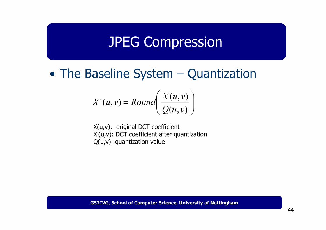
JPEG Compression
=
),(),(),('vuQvuXRoundvuX
X(u,v): original DCT coefficientX’(u,v): DCT coefficient after quantizationQ(u,v): quantization value
• The Baseline System – Quantization
45G52IVG, School of Computer Science, University of Nottingham
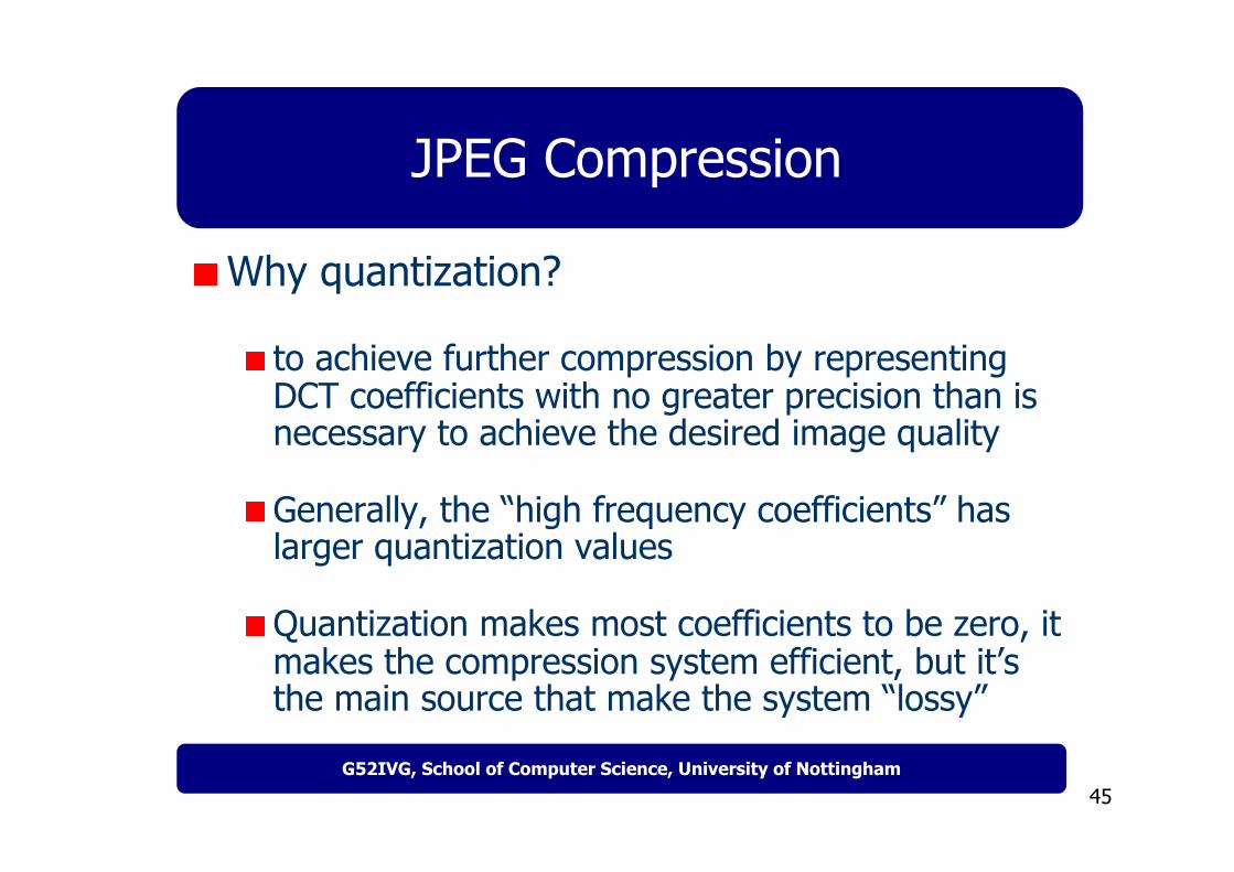
JPEG Compression
Why quantization?
to achieve further compression by representing DCT coefficients with no greater precision than is necessary to achieve the desired image quality
Generally, the “high frequency coefficients” has larger quantization values
Quantization makes most coefficients to be zero, it makes the compression system efficient, but it’s the main source that make the system “lossy”
46G52IVG, School of Computer Science, University of Nottingham
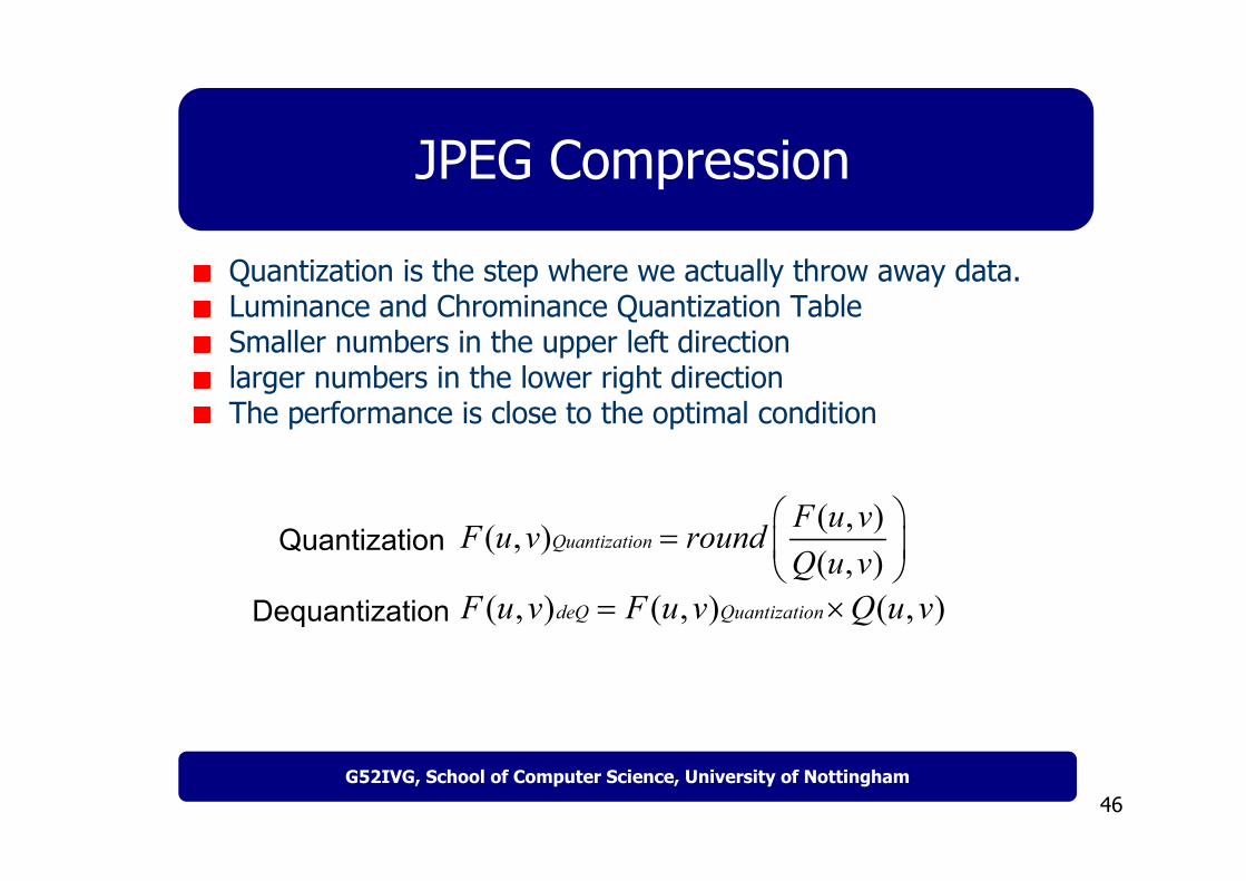
JPEG Compression
Quantization is the step where we actually throw away data.Luminance and Chrominance Quantization Table Smaller numbers in the upper left direction larger numbers in the lower right directionThe performance is close to the optimal condition
( , )( , )( , )
QuantizationF u vF u v roundQ u v
=
( , ) ( , ) ( , )deQ QuantizationF u v F u v Q u v= ×
Quantization
Dequantization

47G52IVG, School of Computer Science, University of Nottingham
JPEG Compression
( , )( , )( , )
QuantizationF u vF u v roundQ u v
=
( , ) ( , ) ( , )deQ QuantizationF u v F u v Q u v= ×
Quantization
Dequantization
16 11 10 16 24 40 51 6112 12 14 19 26 58 60 5514 13 16 24 40 57 69 5614 17 22 29 51 87 80 6218 22 37 56 68 109 103 7724 35 55 64 81 104 113 9249 64 78 87 103 121 120 10172 92 95 98 112 100 103 99
YQ
=
17 18 24 47 99 99 99 9918 21 26 66 99 99 99 9924 26 56 99 99 99 99 9947 66 99 99 99 99 99 9999 99 99 99 99 99 99 9999 99 99 99 99 99 99 9999 99 99 99 99 99 99 9999 99 99 99 99 99 99 99
CQ
=

48G52IVG, School of Computer Science, University of Nottingham
JPEG Compression
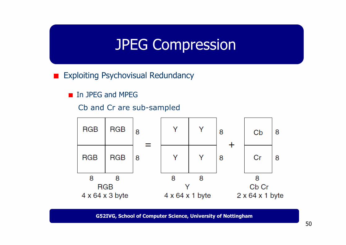
Exploiting Psychovisual Redundancy
Exploit variable sensitivity of humans to colors:
We’re more sensitive to differences between dark intensities than bright ones.
Encode log(intensity) instead of intensity.
We’re more sensitive to high spatial frequencies of green than red or blue.
Sample green at highest spatial frequency, blue at lowest.
We’re more sensitive to differences of intensity in green than red or blue.
Use variable quantization: devote most bits to green, fewest to blue.

49G52IVG, School of Computer Science, University of Nottingham
JPEG Compression
Exploiting Psychovisual Redundancy
NTSC Video
Y bandlimited to 4.2 MHzI to 1.6 MHzQ to .6 MHz
50G52IVG, School of Computer Science, University of Nottingham
JPEG Compression
Exploiting Psychovisual Redundancy
In JPEG and MPEG
Cb and Cr are sub-sampled