Embed Size (px)
Citation preview

Image classification
16-385 Computer VisionSpring 2020, Lecture 18http://www.cs.cmu.edu/~16385/

• Programming assignment 4 is due tonight at 23:59.- Please make sure to download the updated version of PA4 (last updated
Monday, 10 am ET).- Due Wednesday March 25th.- Any questions about the homework?
• Programming assignment 5 will be posted tonight and will be due April 8th.
• Take-home quiz 7 posted and is due Sunday March 29th.
Course announcements

• Introduction to learning-based vision.
• Image classification.
• Bag-of-words.
• K-means clustering.
• Classification.
• K nearest neighbors.
• Naïve Bayes.
• Support vector machine.
Overview of today’s lecture

Slide credits
Most of these slides were adapted from:
• Kris Kitani (16-385, Spring 2017).
• Noah Snavely (Cornell University).
• Fei-Fei Li (Stanford University).

1. Image processing.
2. Geometry-based vision.
3. Physics-based vision.
4. Learning-based vision.
5. Dealing with motion.
Course overview
Lectures 14 – 17
See also 16-823: Physics-based Methods in Vision
See also 15-463: Computational Photography
Lectures 7 – 13
See also 16-822: Geometry-based Methods in Vision
Lectures 1 – 7
See also 18-793: Image and Video Processing
We are starting this part now

What do we mean by learning-
based vision or ‘semantic vision’?

Is this a street light?
(Recognition / classification)

Where are the people?
(Detection)

Is that Potala palace?
(Identification)

What’s in the scene?
(semantic segmentation)
Building
Mountain
Trees
VendorsPeople
Ground
Sky

Object categorization
mountain
building
tree
banner
vendor
people
street lamp

What type of scene is it?
(Scene categorization)
Outdoor
City
Marketplace

Activity / Event Recognition
what are these people doing?

Object recognitionIs it really so hard?
This is a chair
Find the chair in this image Output of normalized correlation
Object recognitionIs it really so hard?
Find the chair in this image
Pretty much garbageSimple template matching is not going to make it
A “popular method is that of template matching, by point to point correlation of a model pattern with the image pattern. These techniques are inadequate for three-dimensional scene analysis for many reasons, such as occlusion, changes in viewing angle, and articulation of parts.” Nivatia & Binford, 1977.

Brady, M. J., & Kersten, D. (2003). Bootstrapped learning of novel objects. J Vis, 3(6), 413-422
And it can get a lot harder

Variability: Camera position
Illumination
Shape parameters
Why is this hard?


Challenge: variable viewpoint
Michelangelo 1475-1564

Challenge: variable illumination
image credit: J. Koenderink

Challenge: scale

Challenge: deformation

Deformation

Challenge: Occlusion
Magritte, 1957

Occlusion

Challenge: background clutter
Kilmeny Niland. 1995
Challenge: Background clutter

Challenge: intra-class variations
Svetlana Lazebnik

Image Classification

Image Classification: Problem

Data-driven approach
• Collect a database of images with labels
• Use ML to train an image classifier
• Evaluate the classifier on test images

Bag of words

What object do these parts belong to?

a collection of local features(bag-of-features)
An object as
Some local feature are
very informative
• deals well with occlusion
• scale invariant
• rotation invariant

(not so) crazy assumption
spatial information of local features
can be ignored for object recognition (i.e., verification)

Csurka et al. (2004), Willamowski et al. (2005), Grauman & Darrell (2005), Sivic et al. (2003, 2005)
Works pretty well for image-level classification
CalTech6 dataset

Bag-of-features
an old idea(e.g., texture recognition and information retrieval)
represent a data item (document, texture, image)
as a histogram over features

Texture recognition
Universal texton dictionary
histogram

Vector Space ModelG. Salton. ‘Mathematics and Information Retrieval’ Journal of Documentation,1979
1 6 2 1 0 0 0 1
Tartan robot CHIMP CMU bio soft ankle sensor
0 4 0 1 4 5 3 2
Tartan robot CHIMP CMU bio soft ankle sensor
http://www.fodey.com/generators/newspaper/snippet.asp

A document (datapoint) is a vector of counts over each word (feature)
What is the similarity between two documents?
counts the number of occurrences just a histogram over words

A document (datapoint) is a vector of counts over each word (feature)
What is the similarity between two documents?
counts the number of occurrences just a histogram over words
Use any distance you want but the cosine distance is fast.

but not all words are created equal

TF-IDF
weigh each word by a heuristic
Term Frequency Inverse Document Frequency
term
frequency
inverse document
frequency
(down-weights common terms)

Standard BOW pipeline(for image classification)

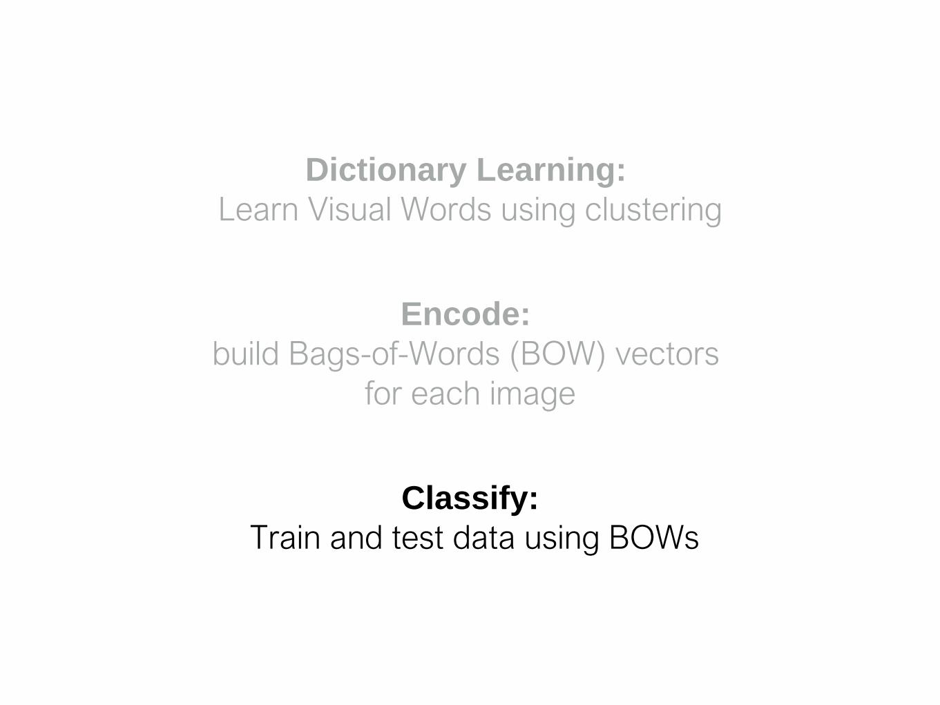
Dictionary Learning:
Learn Visual Words using clustering
Encode:
build Bags-of-Words (BOW) vectors
for each image
Classify:
Train and test data using BOWs

Dictionary Learning:
Learn Visual Words using clustering
1. extract features (e.g., SIFT) from images

Dictionary Learning:
Learn Visual Words using clustering
2. Learn visual dictionary (e.g., K-means clustering)

What kinds of features can we extract?

• Regular grid• Vogel & Schiele, 2003
• Fei-Fei & Perona, 2005
• Interest point detector• Csurka et al. 2004
• Fei-Fei & Perona, 2005
• Sivic et al. 2005
• Other methods• Random sampling (Vidal-Naquet &
Ullman, 2002)
• Segmentation-based patches (Barnard et al. 2003)

Normalize patch
Detect patches[Mikojaczyk and Schmid ’02]
[Mata, Chum, Urban & Pajdla, ’02]
[Sivic & Zisserman, ’03]
Compute SIFT descriptor
[Lowe’99]

…

How do we learn the dictionary?

…

Clustering
…
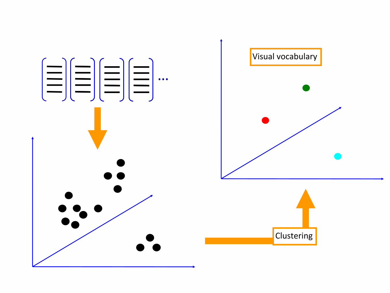
Clustering
…Visual vocabulary

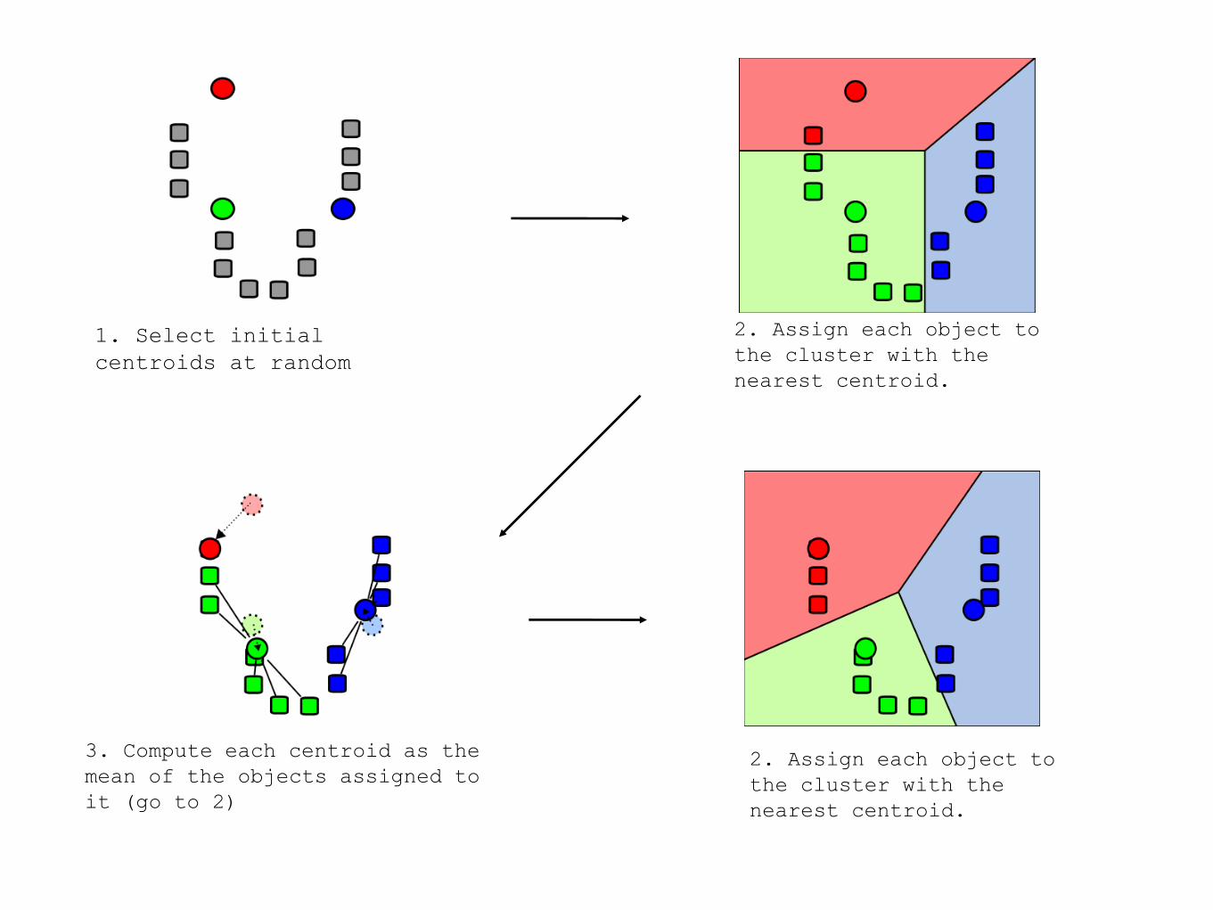
K-means clustering

1. Select initial
centroids at random

1. Select initial
centroids at random
2. Assign each object to
the cluster with the
nearest centroid.

1. Select initial
centroids at random
2. Assign each object to
the cluster with the
nearest centroid.
3. Compute each centroid as the
mean of the objects assigned to
it (go to 2)
1. Select initial
centroids at random
2. Assign each object to
the cluster with the
nearest centroid.
3. Compute each centroid as the
mean of the objects assigned to
it (go to 2)
2. Assign each object to
the cluster with the
nearest centroid.

1. Select initial
centroids at random
2. Assign each object to
the cluster with the
nearest centroid.
3. Compute each centroid as the
mean of the objects assigned to
it (go to 2)
2. Assign each object to
the cluster with the
nearest centroid.
Repeat previous 2 steps until no change

K-means Clustering
Given k:
1.Select initial centroids at random.
2.Assign each object to the cluster with the nearest
centroid.
3.Compute each centroid as the mean of the objects
assigned to it.
4.Repeat previous 2 steps until no change.

From what data should I learn the dictionary?
• Codebook can be learned on separate training set
• Provided the training set is sufficiently
representative, the codebook will be “universal”

From what data should I learn the dictionary?
• Dictionary can be learned on separate training set
• Provided the training set is sufficiently
representative, the dictionary will be “universal”

Example visual dictionary
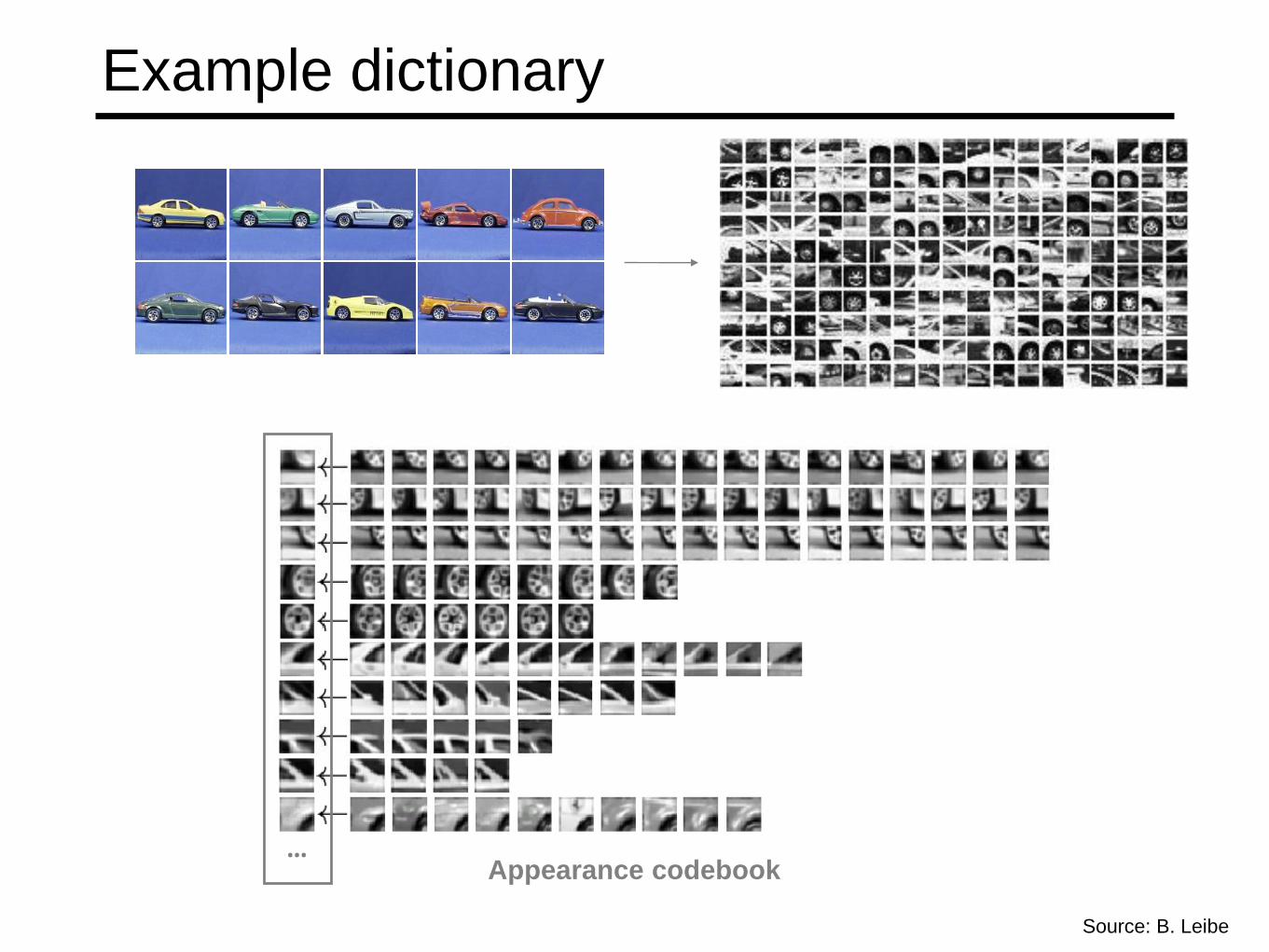
Example dictionary
…
Source: B. Leibe
Appearance codebook
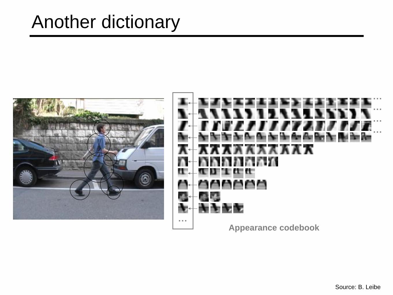
Another dictionary
Appearance codebook…
…
……
…
Source: B. Leibe

Dictionary Learning:
Learn Visual Words using clustering
Encode:
build Bags-of-Words (BOW) vectors
for each image
Classify:
Train and test data using BOWs

Encode:
build Bags-of-Words (BOW) vectors
for each image
1. Quantization: image features gets
associated to a visual word (nearest
cluster center)

Encode:
build Bags-of-Words (BOW) vectors
for each image 2. Histogram: count the
number of visual word
occurrences

…..
freq
uen
cy
codewords
Dictionary Learning:
Learn Visual Words using clustering
Encode:
build Bags-of-Words (BOW) vectors
for each image
Classify:
Train and test data using BOWs

K nearest neighbors
Naïve Bayes
Support Vector Machine

K nearest neighbors

Distribution of data from two classes

Which class does q belong too?
Distribution of data from two classes

Distribution of data from two classes
Look at the neighbors
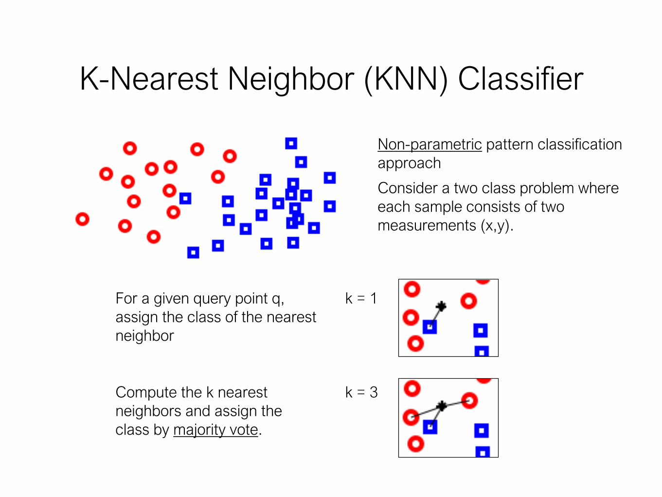
K-Nearest Neighbor (KNN) Classifier
Non-parametric pattern classification
approach
Consider a two class problem where
each sample consists of two
measurements (x,y).
k = 1
k = 3
For a given query point q,
assign the class of the nearest
neighbor
Compute the k nearest
neighbors and assign the
class by majority vote.

Nearest Neighbor is competitive
MNIST Digit Recognition
– Handwritten digits
– 28x28 pixel images: d = 784
– 60,000 training samples
– 10,000 test samples
Test Error Rate (%)
Linear classifier (1-layer NN) 12.0
K-nearest-neighbors, Euclidean 5.0
K-nearest-neighbors, Euclidean, deskewed 2.4
K-NN, Tangent Distance, 16x16 1.1
K-NN, shape context matching 0.67
1000 RBF + linear classifier 3.6
SVM deg 4 polynomial 1.1
2-layer NN, 300 hidden units 4.7
2-layer NN, 300 HU, [deskewing] 1.6
LeNet-5, [distortions] 0.8
Boosted LeNet-4, [distortions] 0.7Yann LeCunn

What is the best distance metric between data points?
• Typically Euclidean distance
• Locality sensitive distance metrics
• Important to normalize. Dimensions have different scales
How many K?
• Typically k=1 is good
• Cross-validation (try different k!)

Distance metrics
Cosine
Chi-squared
Euclidean

Choice of distance metric
• Hyperparameter

Visualization: L2 distance

CIFAR-10 and NN results
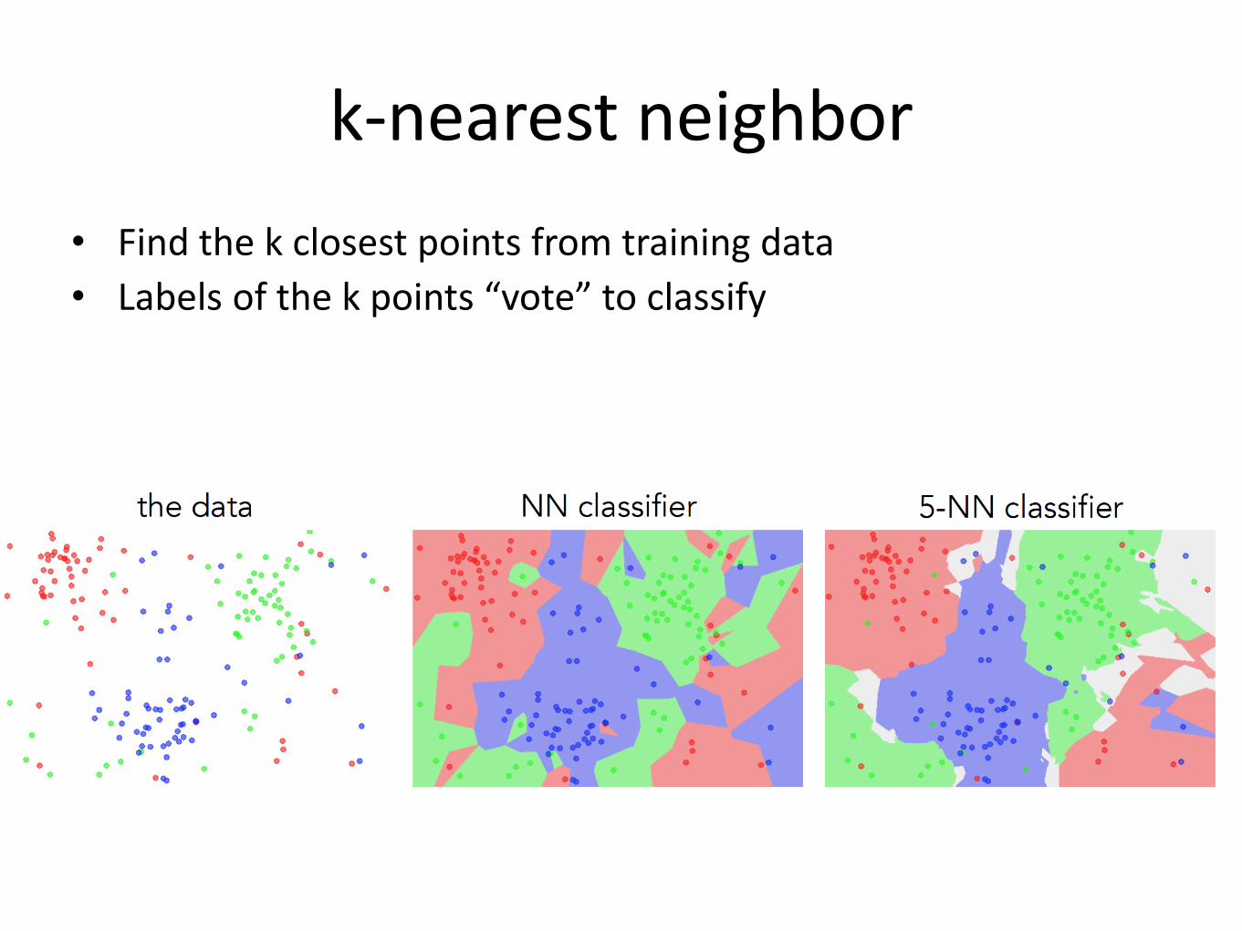
k-nearest neighbor
• Find the k closest points from training data
• Labels of the k points “vote” to classify

Hyperparameters
• What is the best distance to use?
• What is the best value of k to use?
• i.e., how do we set the hyperparameters?
• Very problem-dependent
• Must try them all and see what works best


Validation

Cross-validation


How to pick hyperparameters?
• Methodology
– Train and test
– Train, validate, test
• Train for original model
• Validate to find hyperparameters
• Test to understand generalizability

Pros
• simple yet effective
Cons
• search is expensive (can be sped-up)
• storage requirements
• difficulties with high-dimensional data

kNN -- Complexity and Storage
• N training images, M test images
• Training: O(1)
• Testing: O(MN)
• Hmm…
– Normally need the opposite
– Slow training (ok), fast testing (necessary)


Naïve Bayes

Which class does q belong too?
Distribution of data from two classes

Distribution of data from two classes
• Learn parametric model for each class
• Compute probability of query

This is called the posterior.
the probability of a class z given the observed features X
For classification, z is a
discrete random variable(e.g., car, person, building)
X is a set of observed features(e.g., features from a single image)
(it’s a function that returns a single probability value)

Each x is an observed feature (e.g., visual words)
(it’s a function that returns a single probability value)
This is called the posterior:
the probability of a class z given the observed features X
For classification, z is a
discrete random variable(e.g., car, person, building)

posterior
likelihood prior
The posterior can be decomposed according to
Bayes’ Rule
In our context…
Recall:

The naive Bayes’ classifier is solving this optimization
MAP (maximum a posteriori) estimate
Bayes’ Rule
Remove constants
To optimize this…we need to compute this
Compute the likelihood…

A naive Bayes’ classifier assumes all features are
conditionally independent
Recall:

To compute the MAP estimate
Given (1) a set of known parameters
Compute which z has the largest probability
(2) observations

count 1 6 2 1 0 0 0 1
word Tartan robot CHIMP CMU bio soft ankle sensor
p(x|z) 0.09 0.55 0.18 0.09 0.0 0.0 0.0 0.09
* typically add pseudo-counts (0.001)
** this is an example for computing the likelihood, need to multiply times prior to get posterior
Numbers get really small so use log probabilities

count 1 6 2 1 0 0 0 1
word Tartan robot CHIMP CMU bio soft ankle sensor
p(x|z) 0.09 0.55 0.18 0.09 0.0 0.0 0.0 0.09
count 0 4 0 1 4 5 3 2
word Tartan robot CHIMP CMU bio soft ankle sensor
p(x|z) 0.0 0.21 0.0 0.05 0.21 0.26 0.16 0.11http://www.fodey.com/generators/newspaper/snippet.asp
log p(X|z=grand challenge) = - 14.58
log p(X|z=bio inspired) = - 37.48
log p(X|z=grand challenge) = - 94.06
log p(X|z=bio inspired) = - 32.41
* typically add pseudo-counts (0.001)
** this is an example for computing the likelihood, need to multiply times prior to get posterior

Support Vector Machine

Image Classification

Score function

Linear Classifier
data (histogram)

Convert image to histogram representation

Which class does q belong too?
Distribution of data from two classes

Distribution of data from two classes
Learn the decision boundary

First we need to understand hyperplanes…

Hyperplanes (lines) in 2D
a line can be written as
dot product plus a bias
another version, add a weight 1 and
push the bias inside

Hyperplanes (lines) in 2D
(offset/bias outside) (offset/bias inside)

define the same line
The line
and the line
Important property:
Free to choose any normalization of w
Hyperplanes (lines) in 2D
(offset/bias outside) (offset/bias inside)
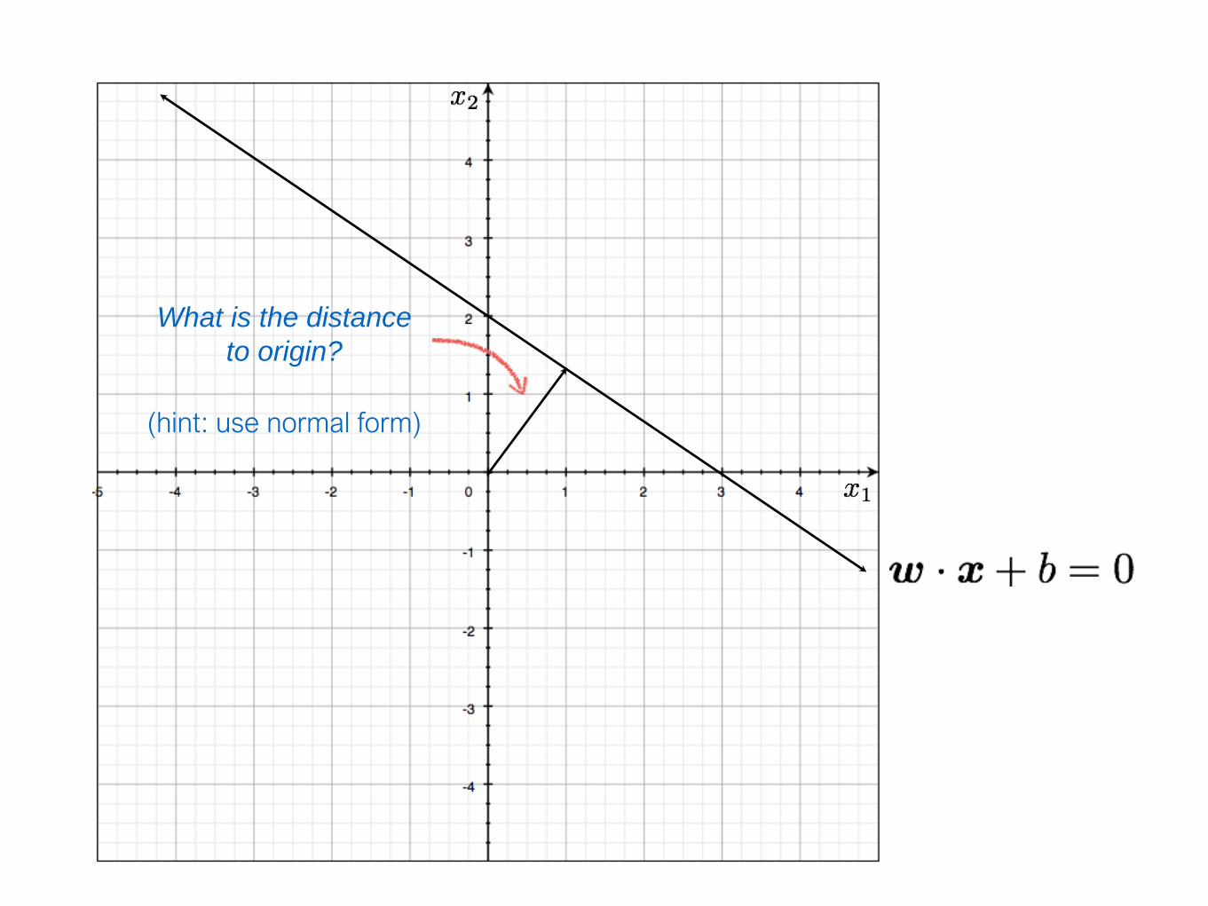
What is the distance
to origin?
(hint: use normal form)

you get the normal form
distance to origin
scale by

What is the distance
between two parallel lines?(hint: use distance to origin)

distance
between two
parallel lines
Difference of distance to origin
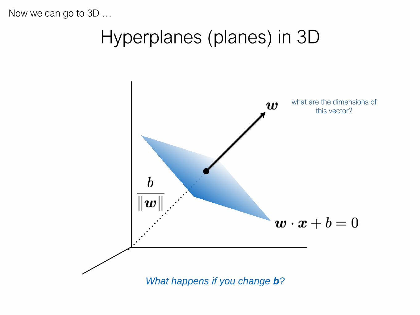
What happens if you change b?
Hyperplanes (planes) in 3D
Now we can go to 3D …
what are the dimensions of
this vector?

Hyperplanes (planes) in 3D

What’s the distance
between these
parallel planes?
Hyperplanes (planes) in 3D

Hyperplanes (planes) in 3D

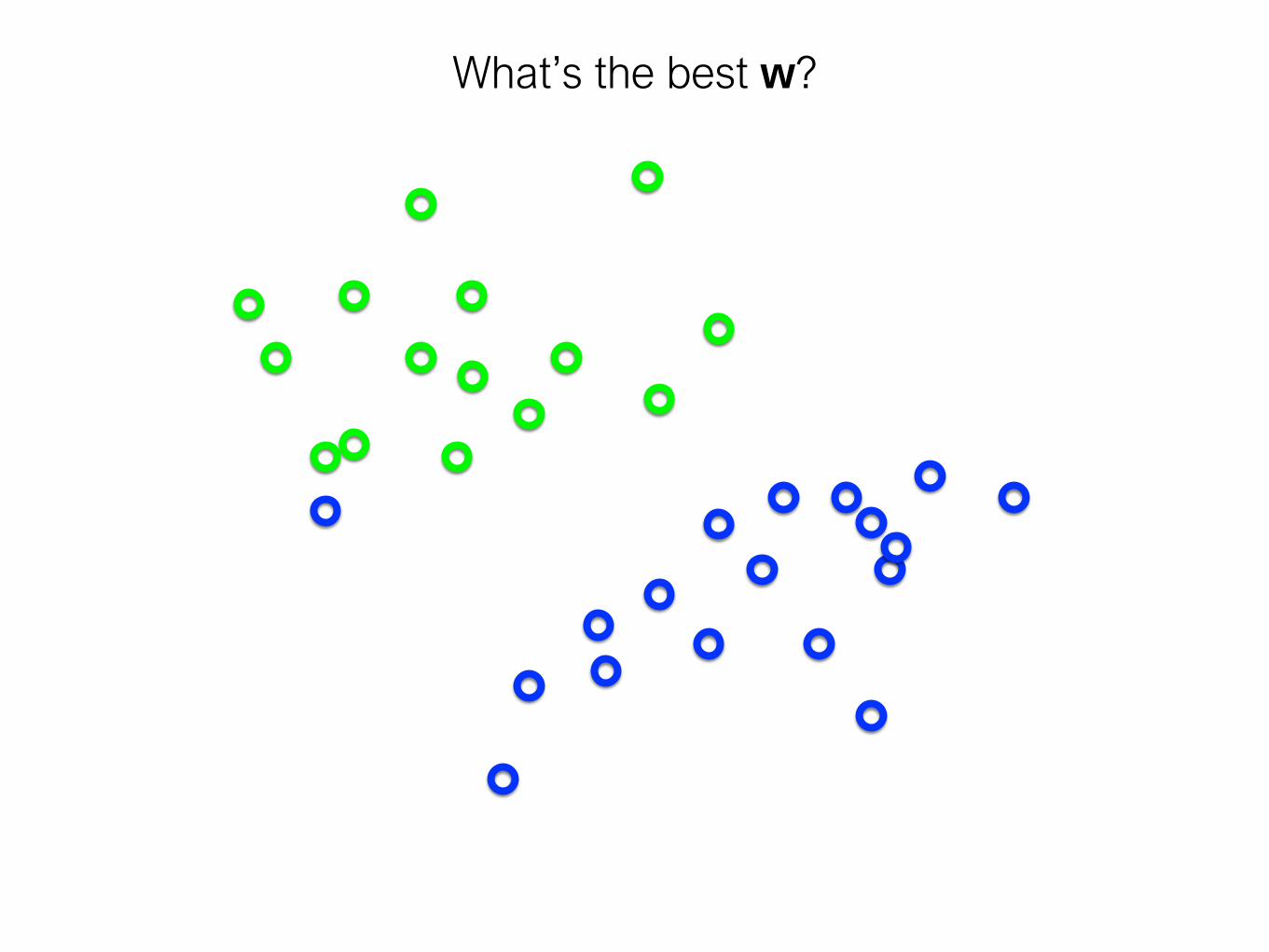
What’s the best w?

What’s the best w?

What’s the best w?

What’s the best w?

What’s the best w?

What’s the best w?
Intuitively, the line that is the
farthest from all interior points

What’s the best w?
Maximum Margin solution:
most stable to perturbations of data

What’s the best w?
Want a hyperplane that is far away from ‘inner points’
support vectors

Find hyperplane w such that …
the gap between parallel hyperplanes
margin
is maximized

Can be formulated as a maximization problem
label of the data point
Why is it +1 and -1?
What does this constraint mean?
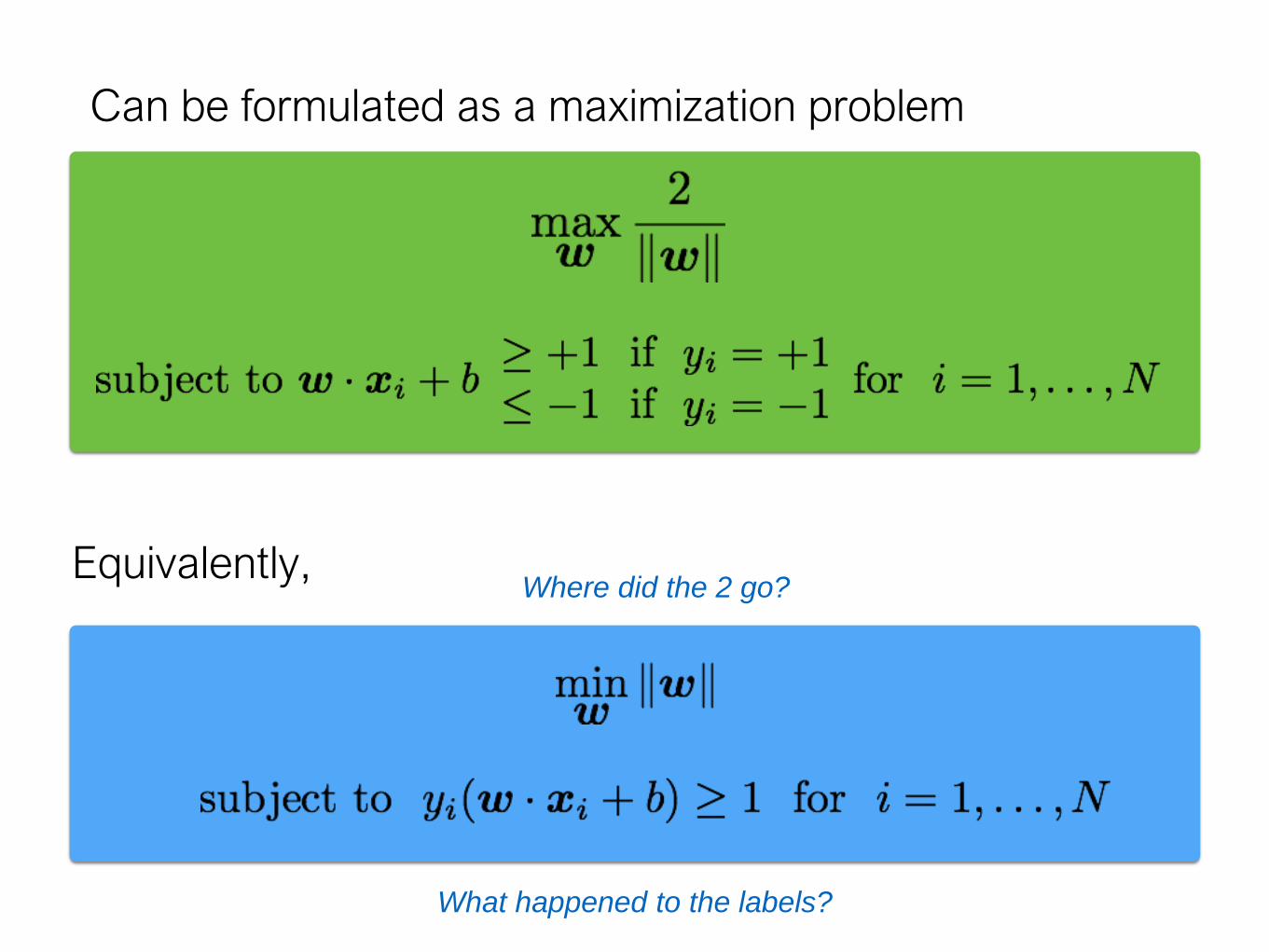
Can be formulated as a maximization problem
Equivalently,Where did the 2 go?
What happened to the labels?
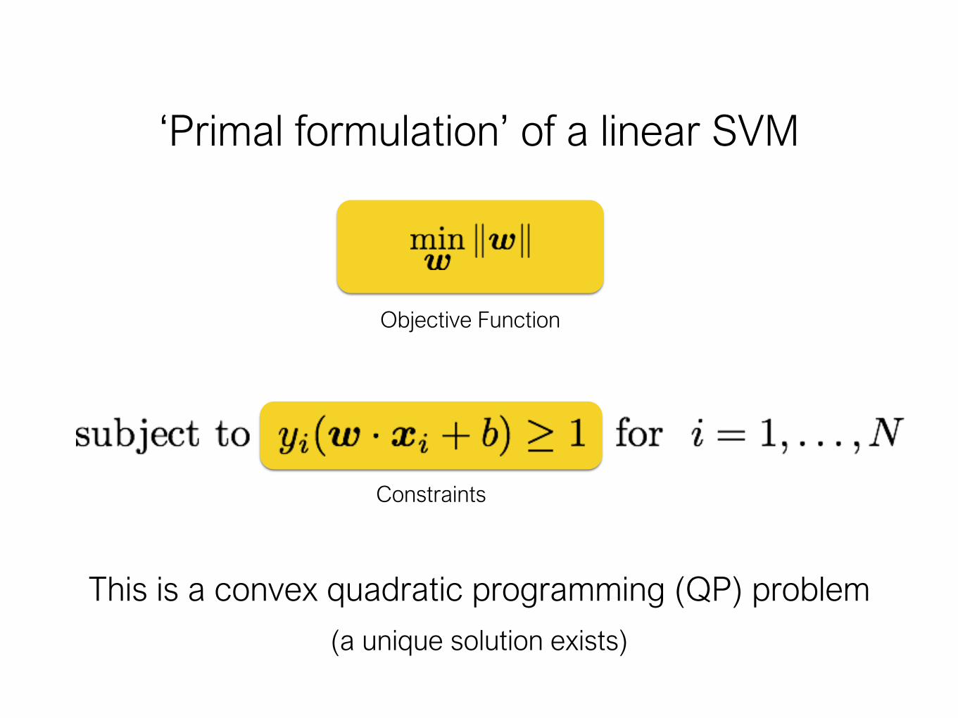
Objective Function
Constraints
‘Primal formulation’ of a linear SVM
This is a convex quadratic programming (QP) problem
(a unique solution exists)

‘soft’ margin
What’s the best w?

What’s the best w?
Very narrow margin

Separating cats and dogs
Very narrow margin

What’s the best w?
Very narrow margin
Intuitively, we should allow for some misclassification if we
can get more robust classification
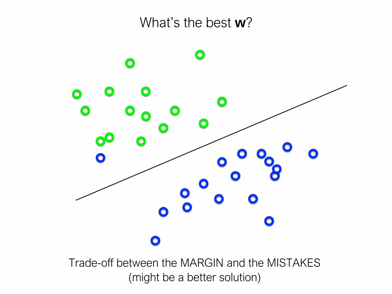
What’s the best w?
Trade-off between the MARGIN and the MISTAKES
(might be a better solution)

Adding slack variables
misclassified
point

‘soft’ margin
objective subject to
for

‘soft’ margin
objective subject to
for
The slack variable allows for mistakes,
as long as the inverse margin is minimized.

‘soft’ margin
subject to
for
objective
• Every constraint can be satisfied if slack is large
• C is a regularization parameter
• Small C: ignore constraints (larger margin)
• Big C: constraints (small margin)
• Still QP problem (unique solution)


References
Basic reading:• Szeliski, Chapter 14.