Image-based Tracking Methods - Applications to Improved Motion Compensation in

Cardiac MR and Image-Guided Surgery

by

Maneesh Dewan

A dissertation submitted to The Johns Hopkins University in conformity with the requirements for the

degree of Doctor of Philosophy.

Baltimore, Maryland

September, 2007

c© Maneesh Dewan 2007

All rights reserved

Abstract

In this dissertation, we present our efforts in developing algorithms in three related

areas: 1) unified and optimal tracking, 2) improved motion compensation in cardiovascular

MR, and 3) tool tracking in image-guided surgery.

With the rapid advancement in the development of tracking algorithms over the years,

the choice of tracking methods for a particular application has significantly increased, but it is

generally not clear what is the best algorithm to use. Recently popularized sampling kernels

have emerged as a flexible design space for developing and merging various tracking algo-

rithms. We demonstrate a connection between kernel-based algorithms and more traditional

template tracking methods. This allows for a more efficient optimization (convergence in fewer

steps) and naturally extends to objective functions optimizing more complex motion models

using multiple spatially distributed kernels. The efficacy of the multi-kernel methods is demon-

strated on a variety of tracking examples. In conventional kernel-based tracking approaches,

the kernel parameters are selected in an ad-hoc fashion usually leading to sub-optimal track-

ing results. Thus, we present results pointing toward the design of optimal and approximately

optimal target-specific kernels for tracking. In image-guided robot-assisted eye surgery, the dy-

namic reconstruction of the surgical field that involves the surgical tools and retinal surface and

ii

features can greatly improve the effectiveness of human-machine cooperative systems that we

have been developing in the Johns Hopkins Engineering Research Center. Thus, we extend the

multiple kernel ideas to develop a generic algorithm for reliably tracking thin surgical tools in

highly textured backgrounds.

Current methods for MR imaging of the cardiac structures, for example coronary ar-

teries and cardiac valves, are limited by the motion artifacts induced by the complex motion

of these structures. We present subject-specific motion compensation techniques to improve

the speed, quality and reliability of imaging cardiac structures in MR. The underlying prin-

ciple involves tracking the cardiac structures in motion affected MR images. Thus, we have

developed a multiple template-based tracking method to track these cardiac structures reliably

and accurately in a range of MR images. Additionally, we have demonstrated the effectiveness

and feasibility of the motion compensation approaches for both coronary MR angiography and

cardiac valve MR imaging.

Primary Advisor: Professor Gregory D. Hager, Department of Computer Science, Johns Hop-

kins University

Advisor/Industrial Collaborator: Dr. Christine H. Lorenz, Siemens Corporate Research and

Department of Radiology and Radiological Sciences, Johns Hopkins University

Reader: Assistant Professor Noah H. Cowan, Department of Mechanical Engineering, Johns

Hopkins University

iii

Acknowledgements

I would like to thank my academic advisor, Professor Gregory Hager for his excellent

guidance and support over the last five years. I am extremely grateful to him for giving me

the freedom to work on various research problems and teaching me the importance of striking a

balance between the nitty-gritty details and the “big picture”. I am also grateful to my co-advisor

and industrial collaborator, Dr. Christine Lorenz for being a great mentor over the last three

years, from whom I have learned a lot about MR techniques and human physiology. I would

also like to thank her for giving me an opportunity to work on an open research problem during

my summer internship at Siemens Corporate Research (SCR) three years ago that materialized

into my dissertation topic.

I wish to thank Professor Noah Cowan for both, introducing me to the world of sensor-

based control and being a reader on my thesis. The class “Sensor based locomotion and manip-

ulation” taught by him has been one of the most enjoyable classes I have taken at Hopkins. I

am also grateful to Professor Russell Taylor for giving me the opportunity to TA the “Computer

Integrated Surgery” class that really helped me grow as a tutor. I am also thankful to Profes-

sor Taylor and Professor Jerry Prince for sitting on my GBO. My thanks also goes to all the

other faculty in the Engineering Research Center (ERC) at Hopkins: Allison Okamura, Gabor

Fichtinger and Peter Kazanzides for their help and support in the last five years. I am also in-

iv

debted to the ERC and CS Department staff, in particular Luwanna Spells and Debbie DeFord

for all their assistance during my stay at Hopkins.

During my PhD, I have been fortunate to be part of the Computational Interaction

and Robotics Lab (CIRL) and the ERC at Hopkins, where I have found great collaborators and

friends. I am grateful to Dr. Jason Corso for his willingness to discuss research problems and

his help in various areas spanning from fixing cameras and code to proof reading papers. I

thank Dr. Panadda Marayong for her camaraderie, and eagerness to help in problems; both

technical and non-technical. Special thanks to Henry Lin with whom I had the opportunity to

develop my teaching skills through intersession courses and the various interesting discussions

about career and life. My thanks also goes to other present and alumni CIRL members - Dr.

Darius Burschka, Tiffany Chen, Dr. Xiangtian Dai, Ioana Fleming, Dr. Le Lu, Stephen Lee,

Dan Mirota, Zachary Pezzementi, Dr. Nicholas Ramey, Carol Reiley, Sharmishtaa Seshamani,

Balazs Vagvolgyi, and Dr. Guangqi Ye, for all their help and the good times I have spent here.

I also thank the rest of the basement ERC crew - Dr. Emad Boctor, Gouthami Chintalapani,

Pezhmann Foroughi, Dr. Ameet Jain, Dr. Ankur Kapoor, Dr. Ming Li, Hassan Rivaz, Sunipa

Saha and Siddharth Vikal, for making my stay at Hopkins memorable. I am grateful to the

LIMBS lab, especially Vinutha Kallem and John Swensen for sharing their interest in robotics

and control. Special thanks to our small DSG group that really helped me survive the thesis

writing ordeal.

I would like to extend my warmest thanks to the Siemens Baltimore Group not only for

their help and encouragement but also providing me with a temporary desk space in a naturally-

lit room. I have been very lucky to work with and learn from both MR scientists and software

engineers in the group - Michael Caylus, Dr. Wesley Gilson, Klaus Kirchberg, Corinna Maier,

v

Glenn Meredith, Dr. Li Pan, and Dr. Steven Shea, to whom I owe my sincere gratitude. I am

also thankful to Andreas Greiser and David Mayhew for making the cardiac valve MR imaging

project realizable.

I have had the pleasure of enjoying the company of some incredible friends outside of

my work, during my stay at Hopkins. The wonderful times spent with Jatin Chhugani, Vikram

Krishnaswamy, Mauktik Kulkarni, Mihir Naware, Abhishek Rege, Dheeraj Singaraju, and

Pramodsingh Thakur, will always stay in my memories. To this day, it surprises me how they

were able to survive my eccentricities; especially, the singing with self-made lyrics, the high-

pitched voice and the Indian lentil cooking. My thanks also goes to Harsh Agarwal, Nirveek

Bhattacharya, Sachin Chandran, Anoop Deoras, Barun Maskara, Sarthak Mishra, Vaishali Pali-

wal, Amit Paliwal, Saurav Panda, Neeraja Penumetcha, Anshumal Sinha, and Karthik Vish-

wanathan for sharing a lot of their time with me.

In the end, I would like to extend my deepest gratitude to my parents and my family in

India and US, for their unconditional support throughout my PhD. My cousins Amisha, Amit,

Anupama, Kamini, Parag, Poshak, Naully, Raveesh, Ritesh and Tapan have always shown faith

in me and have stood by me during the ups and downs of my PhD. Finally, I would like to

dedicate the thesis to my parents, Sharda and Surinder Kumar Dewan, without whose constant

love, understanding and encouragement, I would not have made it this far.

Maneesh Dewan

Baltimore,

21 September 2007.

vi

Contents

Abstract ii

Acknowledgements iv

List of Figures ix

List of Tables xiv

1 Introduction 11.1 Motivation . . . . . . . . . . . . . . . . . . . . . . . . . . . . . . . . . . . . . . . . . . 41.2 Thesis Contributions and Overview . . . . . . . . . . . . . . . . . . . . . . . . . . . . . 10

1.2.1 Contributions - Tracking Methods . . . . . . . . . . . . . . . . . . . . . . . . . 101.2.2 Contributions - Improved Motion Compensation in Cardiovascular MR . . . . . 111.2.3 Contributions - Tool Tracking in Image-guided Eye Surgery . . . . . . . . . . . 13

2 Tracking Methods 142.1 Kernel-based Tracking . . . . . . . . . . . . . . . . . . . . . . . . . . . . . . . . . . . 17

2.1.1 Background . . . . . . . . . . . . . . . . . . . . . . . . . . . . . . . . . . . . . 172.1.2 Mean-shift formulation . . . . . . . . . . . . . . . . . . . . . . . . . . . . . . . 192.1.3 SSD Formulation . . . . . . . . . . . . . . . . . . . . . . . . . . . . . . . . . . 232.1.4 More Complex Motion Models . . . . . . . . . . . . . . . . . . . . . . . . . . 242.1.5 The Limits of Single Kernels . . . . . . . . . . . . . . . . . . . . . . . . . . . . 272.1.6 Extension to Multiple Kernels . . . . . . . . . . . . . . . . . . . . . . . . . . . 282.1.7 The Relationship Between Spatial Structure and Kernel Structure . . . . . . . . 312.1.8 Multiple Kernel Constructions . . . . . . . . . . . . . . . . . . . . . . . . . . . 322.1.9 Demonstrations . . . . . . . . . . . . . . . . . . . . . . . . . . . . . . . . . . . 352.1.10 Structured Tracking Example - Tool Tracking for Image-guided Retinal

Surgery . . . . . . . . . . . . . . . . . . . . . . . . . . . . . . . . . . . . . . . 392.2 Multiple Template Tracking . . . . . . . . . . . . . . . . . . . . . . . . . . . . . . . . 44

2.2.1 Background . . . . . . . . . . . . . . . . . . . . . . . . . . . . . . . . . . . . . 442.2.2 Affine-weighted SSD formulation . . . . . . . . . . . . . . . . . . . . . . . . . 472.2.3 Extension to Bidirectional Methods . . . . . . . . . . . . . . . . . . . . . . . . 502.2.4 Template Selection . . . . . . . . . . . . . . . . . . . . . . . . . . . . . . . . . 51

2.3 Conclusions . . . . . . . . . . . . . . . . . . . . . . . . . . . . . . . . . . . . . . . . . 53

vii

3 Optimal Kernels 563.1 Background . . . . . . . . . . . . . . . . . . . . . . . . . . . . . . . . . . . . . . . . . 573.2 Problem Formulation . . . . . . . . . . . . . . . . . . . . . . . . . . . . . . . . . . . . 583.3 Simple One Dimensional Case . . . . . . . . . . . . . . . . . . . . . . . . . . . . . . . 623.4 Extension to the Two-Dimensional Case . . . . . . . . . . . . . . . . . . . . . . . . . . 663.5 Conclusions . . . . . . . . . . . . . . . . . . . . . . . . . . . . . . . . . . . . . . . . . 77

4 Beat-to-Beat Motion Compensation for Robust Coronary MR Angiography 784.1 Introduction . . . . . . . . . . . . . . . . . . . . . . . . . . . . . . . . . . . . . . . . . 784.2 Previous Work . . . . . . . . . . . . . . . . . . . . . . . . . . . . . . . . . . . . . . . . 80

4.2.1 Respiratory Motion Variability . . . . . . . . . . . . . . . . . . . . . . . . . . . 824.2.2 Heart Rate and Cardiac Motion Variability . . . . . . . . . . . . . . . . . . . . 83

4.3 Proposed Approach - Image-based Navigators . . . . . . . . . . . . . . . . . . . . . . . 854.4 Data Acquisition . . . . . . . . . . . . . . . . . . . . . . . . . . . . . . . . . . . . . . 894.5 Tracking Algorithm and Validation . . . . . . . . . . . . . . . . . . . . . . . . . . . . . 914.6 Heart Rate Variability . . . . . . . . . . . . . . . . . . . . . . . . . . . . . . . . . . . . 984.7 MR Simulation . . . . . . . . . . . . . . . . . . . . . . . . . . . . . . . . . . . . . . . 994.8 Comparison of Diaphragm and Coronary Motion . . . . . . . . . . . . . . . . . . . . . 1064.9 User Interface (UI) . . . . . . . . . . . . . . . . . . . . . . . . . . . . . . . . . . . . . 109

4.9.1 Initial Testing and Results . . . . . . . . . . . . . . . . . . . . . . . . . . . . . 1104.10 Discussion and Conclusions . . . . . . . . . . . . . . . . . . . . . . . . . . . . . . . . 110

5 Improved Motion Compensation in Cardiac Valve MR Imaging 1175.1 Introduction . . . . . . . . . . . . . . . . . . . . . . . . . . . . . . . . . . . . . . . . . 1175.2 Previous Work . . . . . . . . . . . . . . . . . . . . . . . . . . . . . . . . . . . . . . . . 1195.3 Proposed Approach - Valve Imaging with Image-based Tracking . . . . . . . . . . . . . 1235.4 Validation and Experiments . . . . . . . . . . . . . . . . . . . . . . . . . . . . . . . . . 127

5.4.1 Study I - Tracking Validation . . . . . . . . . . . . . . . . . . . . . . . . . . . . 1275.4.2 Study II - Valve Imaging Comparison . . . . . . . . . . . . . . . . . . . . . . . 131

5.5 Discussion and Conclusions . . . . . . . . . . . . . . . . . . . . . . . . . . . . . . . . 135

6 Conclusions and Future Work 1406.1 Tracking Methods . . . . . . . . . . . . . . . . . . . . . . . . . . . . . . . . . . . . . . 1406.2 Motion Compensation in Cardiovascular MR . . . . . . . . . . . . . . . . . . . . . . . 1426.3 Tracking in Image-guided Surgery . . . . . . . . . . . . . . . . . . . . . . . . . . . . . 1466.4 Future Directions . . . . . . . . . . . . . . . . . . . . . . . . . . . . . . . . . . . . . . 146

Bibliography 148

Vita 164

viii

List of Figures

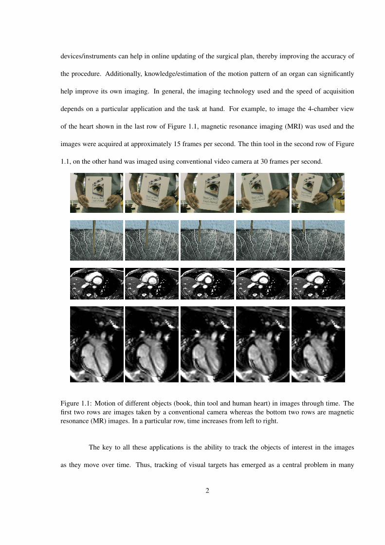
1.1 Motion of different objects (book, thin tool and human heart) in images through time.The first two rows are images taken by a conventional camera whereas the bottom tworows are magnetic resonance (MR) images. In a particular row, time increases from leftto right. . . . . . . . . . . . . . . . . . . . . . . . . . . . . . . . . . . . . . . . . . . . 2

1.2 Left circumflex coronary artery and mitral valve motion through the cardiac cycle in the4-chamber view. The coronary artery is depicted by an orange circle and the valve planeby a green line. . . . . . . . . . . . . . . . . . . . . . . . . . . . . . . . . . . . . . . . 5

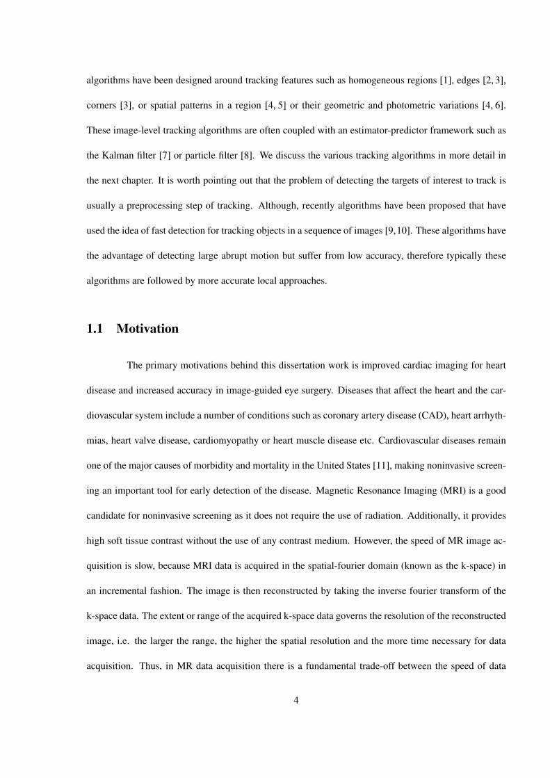
1.3 Importance of motion compensation in MR. Transverse image taken with (A) no motioncompensation, (B) cardiac motion compensation and (C) cardiac and respiratory motioncompensation. The images are taken from [14]. . . . . . . . . . . . . . . . . . . . . . . 6

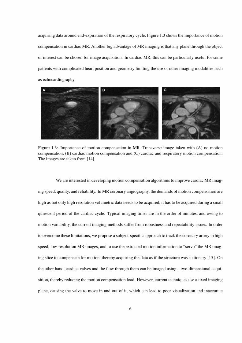
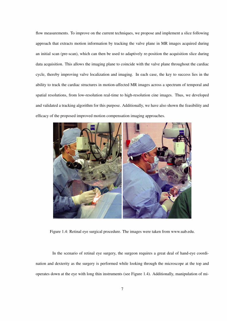
1.4 Retinal eye surgical procedure. The images were taken from www.uab.edu. . . . . . . . 7

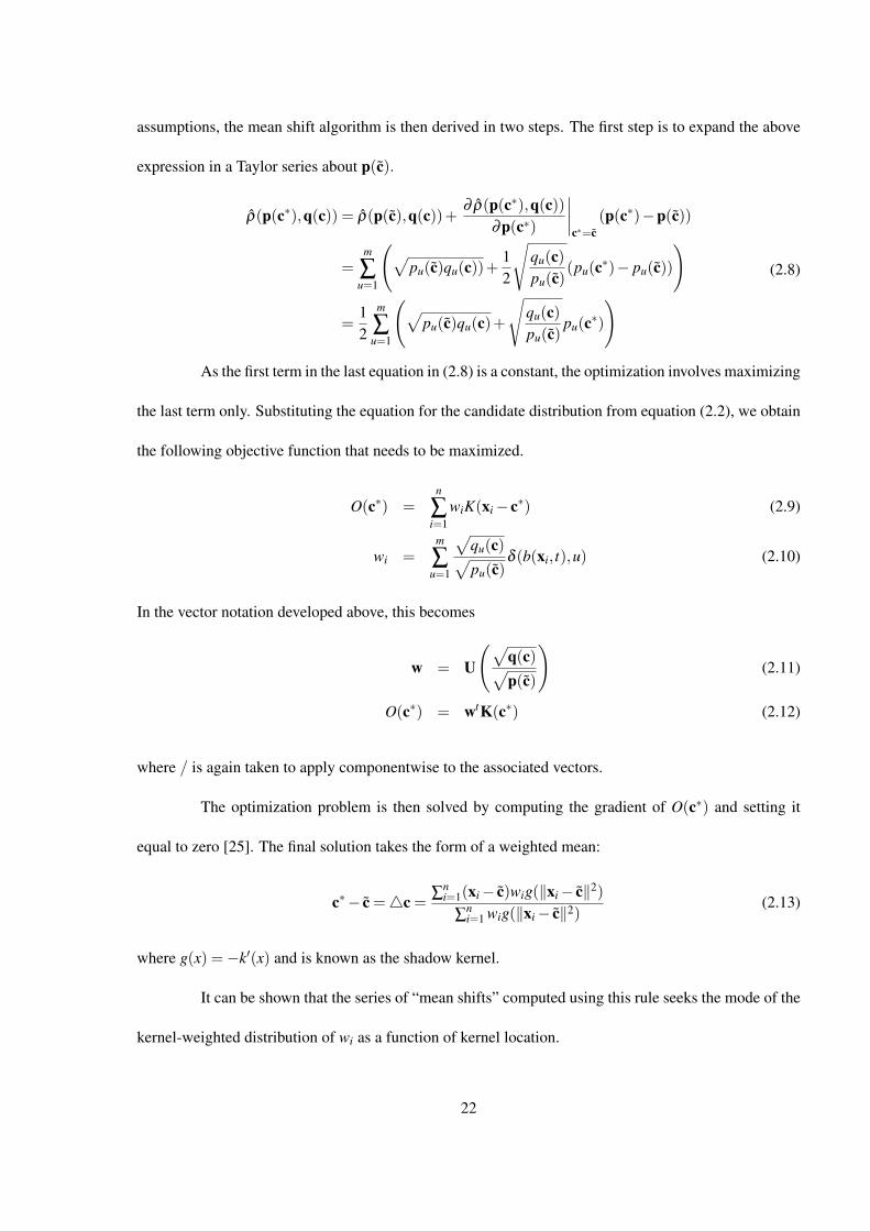
2.1 Steps involved in building a kernel weighted histogram . . . . . . . . . . . . . . . . . . 202.2 Return map comparison between mean shift and kernel-based SSD approach. The left

plot compares the return map for shift when the target is centered on “box” signal; theright plot the performance when the target is centered on a 1D step function (an “edge”).For kernel-based SSD approach, both epan and triangular kernels [46] have been used.It can be seen that SSD has nearly perfect 1-step performance, whereas mean shift muchslower to return. . . . . . . . . . . . . . . . . . . . . . . . . . . . . . . . . . . . . . . . 25

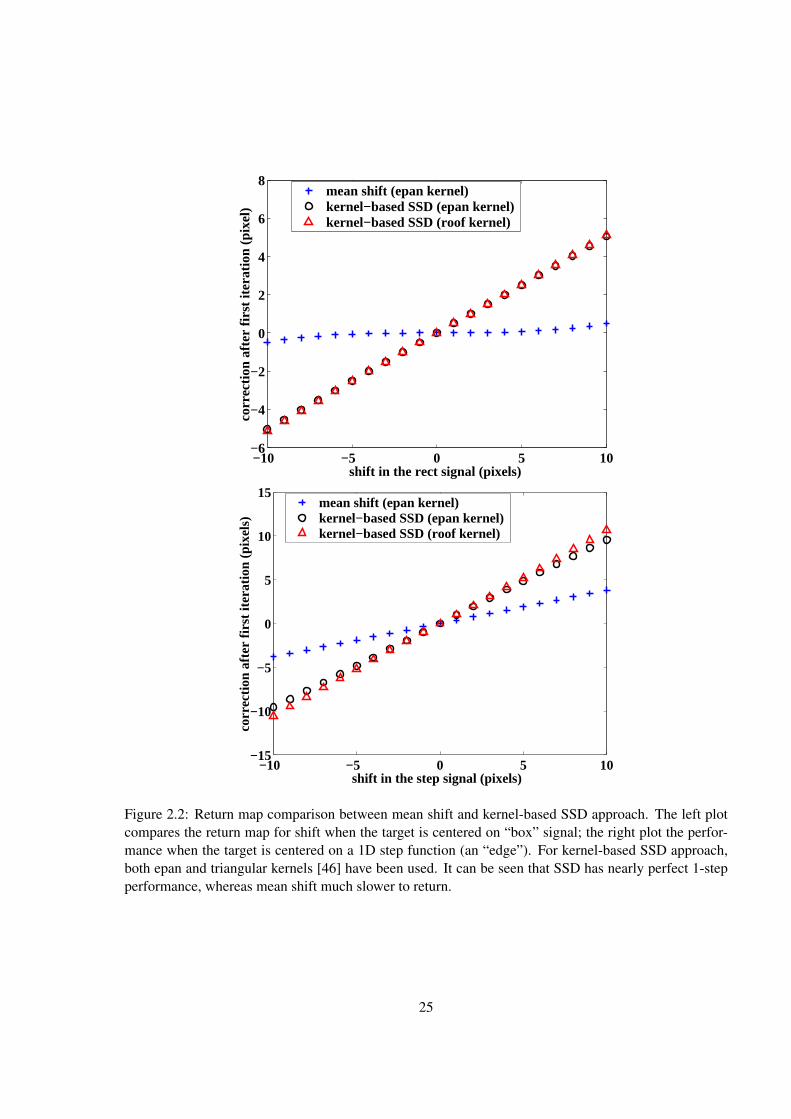
2.3 A tracking on a bulls-eye figure. . . . . . . . . . . . . . . . . . . . . . . . . . . . . . . 272.4 The x and y roof kernels. . . . . . . . . . . . . . . . . . . . . . . . . . . . . . . . . . . 302.5 Tracking on a bulls-eye figure with multiple kernels. . . . . . . . . . . . . . . . . . . . 332.6 Different rotation kernels. The top row shows the kernels in (2.28) and the bottom row

shows the kernels in (2.29). . . . . . . . . . . . . . . . . . . . . . . . . . . . . . . . . . 342.7 The center position of the tracked region for mean shift, single-kernel SSD and the

multiple-kernel SSD with histogram binning based on HSV space (2 iterations per frame). 362.8 The center position of the tracked region for mean shift, single-kernel SSD and the

multiple-kernel SSD with histogram binning based on both HSV and RGB space (2iterations per frame). . . . . . . . . . . . . . . . . . . . . . . . . . . . . . . . . . . . . 37

ix

2.9 Tracking comparison for mean shift, single-kernel SSD and multiple-kernel SSD ap-proaches with 2 iterations per frame. The first frame shows the selected template region.In the following frames (frame numbers 98, 158, 290, 332, and 413) the tracked regionfrom these different tracking approaches are shown. The tracked region in each frame formean shift, single-kernel SSD and multiple-kernel SSD with histogram binning based onHSV space are shown in blue, red and green rectangle respectively. The tracked regionwith histogram binning based on RGB space for mean shift and single-kernel SSD areshown in magenta and black respectively. . . . . . . . . . . . . . . . . . . . . . . . . . 38

2.10 Tracking scale and translation with the multi kernel SSD approach. The first frame showsthe selected template region. The subsequent frames i.e. 22, 45, 78, 84 and 98 show thetracked region with a blue rectangle . . . . . . . . . . . . . . . . . . . . . . . . . . . . 40

2.11 Similarity (translation, scale, and rotation) tracking with the multi kernel SSD approach.The tracked region is shown with a blue rectangle . . . . . . . . . . . . . . . . . . . . . 41

2.12 Placement of multiple kernels for tool tracking. The kernel placements are indicated bythe rectangular boxes where the tool is outlined by a dotted yellow line. . . . . . . . . . 43

2.13 Tracking a tool attached to the steady hand robot in the preliminary test-bed for retinaleye surgery [23, 24]. This is the left image of a stereo pair. The tracked frames shown inrest of the rows are frame numbers 130,170,210,250,330 and 410. . . . . . . . . . . . . 44

2.14 Comparison of high resolution cine (left) and realtime low-resolution images (right) in4-chamber (top row) and short axis views (bottom row). The arrow indicates the locationof the left coronary artery. Note that the coronary artery is clearly visible in the highresolution images but blurred out in corresponding real-time images. . . . . . . . . . . . 46

2.15 Mitral and aortic valves in high resolution cine (left) and realtime low-resolution im-ages (right) in 4-chamber (top row) and coronal views (bottom row). The overlaid lineindicates the valve plane. . . . . . . . . . . . . . . . . . . . . . . . . . . . . . . . . . . 46

2.16 Inutition behind multiple template SSD tracking . . . . . . . . . . . . . . . . . . . . . . 492.17 Optimal Templates selected (enclosed in rectangle) from the manually selected 40 tem-

plates. . . . . . . . . . . . . . . . . . . . . . . . . . . . . . . . . . . . . . . . . . . . . 532.18 Tracking comparison with optimal and non-optimal templates. The templates used for

equal-spaced 1 and 2 are (5,20,35) and (1,20,40) respectively. . . . . . . . . . . . . . . . 54

3.1 Return map comparison between kernel-based SSD [27] and optimal kernels on a stepsignal (left). The right plot shows the step signal, the estimated optimal kernels (seesection 3.3) and epan and roof kernels used for kernel-based SSD. Note that in the kernel-based SSD method, the kernel is placed at the center with the scale equal to the size ofthe signal. . . . . . . . . . . . . . . . . . . . . . . . . . . . . . . . . . . . . . . . . . . 59

3.2 Comparison of SSD and optimal kernel methods on an artificial multiple step signal. Thetop and bottom rows show the results using square and gaussian kernels respectively. Auniform model for u is used for both kernels. . . . . . . . . . . . . . . . . . . . . . . . 67

3.3 Comparison of SSD and optimal kernel methods on a real signal with gaussian kernels.Numerical integration with uniform model for u is used. . . . . . . . . . . . . . . . . . 67

3.4 Comparison of SSD and optimal kernel methods on real signals with square kernels. Agaussian model for u is used. One can see the approx 1 works as well as the numericalintegration. . . . . . . . . . . . . . . . . . . . . . . . . . . . . . . . . . . . . . . . . . 68

3.5 Optimization of x-translation kernel Kx(x,y) in 2D. . . . . . . . . . . . . . . . . . . . . 71

x

3.6 Comparison of SSD and optimal kernel methods on a artificial signal in 2D. The rightplot shows the return map in twice the optimized range of u and v. Optimal kernel - 1Dand Optimal kernel - 2D refers to the results using kernels obtained before and after the2D joint optimization. . . . . . . . . . . . . . . . . . . . . . . . . . . . . . . . . . . . . 73

3.7 Location selection using heuristics. The left column shows the 10 pairs generated by theheuristics overlaid on the template. The right column shows the return map comparisons. 74

3.8 Tracking Comparisons between optimal kernels(blue box) and kernel-based SSD [27](ma-genta box). Frames 20, 35, 50, 100, 200 and 300 are shown in order. The kernel-basedSSD tracking fails around frame 40. . . . . . . . . . . . . . . . . . . . . . . . . . . . . 75

3.9 Comparison of rotation and scale estimation with the transformed optimal gaussian ker-nel and SSD Method on the clown image. . . . . . . . . . . . . . . . . . . . . . . . . . 76

4.1 The primary coronary arteries in the heart. . . . . . . . . . . . . . . . . . . . . . . . . . 794.2 Current Approach for coronary MRA. . . . . . . . . . . . . . . . . . . . . . . . . . . . 814.3 Basic sequence-timing diagram of the proposed approach using image-based navigators. 864.4 Process flow in the proposed approach for coronary MRA. . . . . . . . . . . . . . . . . 874.5 Subject-specific heart coordinate system. The X ′, Y ′ and Z′ axes of the heart coordinate

system are shown in 4-chamber and short axis views separately in 2D (a) and in 3D (b). . 884.6 Sequence diagram of a real-time acquisition in cardiac MR. Images are acquired through

time. As the heart is undergoing cardiac and respiratory motion, the time duration of theacquisition of each image is limited therefore the spatial resolution determined by theextent of k-space filled is low. . . . . . . . . . . . . . . . . . . . . . . . . . . . . . . . . 90

4.7 Tracked positions of LCX in the 4-chamber (1st row), and LAD in the short axis (2ndrow) and coronal (3rd row) views at different points in the cardiac cycle. The box repre-sents the tracked region with the dot representing the estimated location of the coronaryartery. . . . . . . . . . . . . . . . . . . . . . . . . . . . . . . . . . . . . . . . . . . . . 93

4.8 Tracked positions of RCA in the 4-chamber view at different points in the cardiac cycle.The box represents the tracked region with the dot representing the estimated location ofthe coronary artery. . . . . . . . . . . . . . . . . . . . . . . . . . . . . . . . . . . . . . 93

4.9 Tracked coronary motion in low resolution real-time images. The top (a) and bottom(b) rows correspond to 4-chamber and short axis views respectively. The left columnshows the transformed heart coordinate system (in gray) whereas the right column showsthe transformed tracked coronary motion of LCX and RCA in 4-chamber and LDA inshort-axis views. The transformed tracked coronary motion plot shows the X ′, Y ′ and Z′

motions. . . . . . . . . . . . . . . . . . . . . . . . . . . . . . . . . . . . . . . . . . . 944.10 Detected end-systolic and end-diastolic time points in the extracted coronary motion data

from a 4-chamber view in a single volunteer over 8 cardiac beats. . . . . . . . . . . . . . 964.11 Comparison of tracked coronary motion from breath-hold real-time acquisition (solid)

with the motion from high resolution segmented cine acquisition (dashed) in coronal(top left), four chamber (top right) and short axis (bottom) views for a one volunteer(out of the 5). In each plot, the top and bottom subplots correspond to x and y motionrespectively. The dashed-dot vertical black line corresponds to the end-systolic time. . . 97

4.12 Variability in the diastolic and systolic periods in 5 volunteers. The duration of the examwas approximately 21, 15, 39, 11 and 10 minutes, respectively for the 5 volunteers. Theerror bars are the standard deviation of each period. . . . . . . . . . . . . . . . . . . . . 99

4.13 Flowchart describing the MR simulation analysis. . . . . . . . . . . . . . . . . . . . . . 99

xi

4.14 Acquisition window selection for adaptive (empty boxes) and fixed (filled boxes) triggerdelays for window width of 65 ms. The solid curve shows the x and y motion profiles (incm). The dotted vertical lines depict the end-systolic time point. The fixed trigger delayacquisition window depicted by the duration between the two filled boxes is calculatedfrom minimum velocity time point in the high resolution cine sequence. The adaptivetrigger delay acquisition window depicted by the duration between the two empty boxesis computed on a beat-to-beat basis as the time point corresponding to the minimumvelocity point in that cardiac cycle. . . . . . . . . . . . . . . . . . . . . . . . . . . . . . 100

4.15 Comparison of adaptive and fixed trigger delays for image acquisition as function of ac-quisition window (in ms) for the simulation analysis. The left and right column showsthe best and worst results in terms of percent gain or loss in SNR of the adaptive delaymethod over the fixed delay method for a particular acquisition window from the set of10 runs for all volunteers in all views (see MR simulation section). 5 most representativeimages out of the 10 are shown. The top and bottom rows in each sub-figure correspondto adaptive and fixed trigger delay case, respectively. Note that the phase encoding andfrequency encoding directions are along the column and row of the image respectively.Note that even in the worst case comparison, the adaptive delay method quality is com-parable to the fixed delay method, while in the best case comparison, the adaptive delaymethod shows significantly better image quality as compared to the fixed delay. . . . . . 104

4.16 SNR (left column) and CNR (right column) comparison between adaptive (dark gray)and fixed (light gray) trigger delays for different acquisition windows for left (a) and right(b) coronary artery. Each plot is a box and whisker plot in MATLAB (Mathworks Inc.).The box has lines at the lower quartile, median, and upper quartile values. The whiskers(dotted lines) are a function of inter-quartile range. The pluses denote the outliers beyondthe whisker range. One can note that as the acquisition window increases, the incrementalbenefit of an adaptive delay is decreased. . . . . . . . . . . . . . . . . . . . . . . . . . . 105

4.17 Comparison of respiratory motion of the lung-diaphragm interface and the LAD coronaryartery in a one (out of the 5) volunteer. The top figure shows the location of the LADand lung-diaphragm interface in the coronal view (dots). The darker and lighter boxesshow the tracked region for lung-diaphragm interface and LAD respectively. The bottomplot shows the motion of the 0.6*lung-diaphragm interface (solid black), total coronarymotion (solid gray) and the respiratory component of the coronary motion (dashed). . . 107

4.18 Comparison of respiratory motion of the lung-diaphragm interface and the LAD coronaryartery in a one (out of the 5) volunteer over a much longer duration of time (approx. aminute). . . . . . . . . . . . . . . . . . . . . . . . . . . . . . . . . . . . . . . . . . . . 108

4.19 Root mean squared error between the respiratory motion of the lung-diaphragm interfaceand the LAD coronary artery for all volunteers. . . . . . . . . . . . . . . . . . . . . . . 108

4.20 Screenshots of the coronary UI. The two screenshots show two (out of the four) toggledviews of the UI. . . . . . . . . . . . . . . . . . . . . . . . . . . . . . . . . . . . . . . . 111

4.21 Screenshots of the online testing with the coronary UI. The top one is on a simple phan-tom whereas the bottom one is in a volunteer. . . . . . . . . . . . . . . . . . . . . . . . 112

5.1 Cardiac valves in the heart. The left image is a slice through the long axis of the heart.The image was taken from www.lifeisnow.com. . . . . . . . . . . . . . . . . . . . . . . 118

5.2 Limitation of conventional cardiac MR valve imaging. The imaging plane (shown ingreen) is fixed through the cardiac cycle whereas the valve plane (shown in yellow)moves in and out of it. . . . . . . . . . . . . . . . . . . . . . . . . . . . . . . . . . . . 120

xii

5.3 Sequence diagram of a cine segmented acquisition. Images throughout the cardiac cycleare acquired. Each image (or its corresponding k-space data) is acquired over multipleheart beats. . . . . . . . . . . . . . . . . . . . . . . . . . . . . . . . . . . . . . . . . . 121

5.4 Tagging of the aortic valve plane in the coronal view through the cardiac cycle. Thetrigger delay time is at the bottom right of every image. The estimated valve plane isshown in solid red line whereas the initial location in the first frame is shown as a dottedred line. Note the fading of the tags towards the end of the cardiac cycle. The image wastaken from [131]. . . . . . . . . . . . . . . . . . . . . . . . . . . . . . . . . . . . . . . 123

5.5 Tagging plane selection for the mitral valve. The tagged plane (shown by the line con-necting the two circular markers) was selected basal to the actual valve plane (shown bythe shaded slab). The image was taken from [130]. . . . . . . . . . . . . . . . . . . . . 123

5.6 Basic flow of the valve imaging approach . . . . . . . . . . . . . . . . . . . . . . . . . 1245.7 Mitral valve tracking in two orthogonal views in a single volunteer. . . . . . . . . . . . . 1255.8 Tracking of the aortic valve in two orthogonal views in a single volunteer. . . . . . . . . 1265.9 Scanner UI task card showing repositioning of the scan planes . . . . . . . . . . . . . . 1265.10 Tracking of mitral (top two rows) and aortic (bottom two rows) valves in low-resolution

real-time images in a two volunteers. Five frames from the 128 frame long sequencefor each view are shown. The (first, third) and (second, fourth) rows belong to the samevolunteers. The valve plane is depicted with a blue line. . . . . . . . . . . . . . . . . . . 128

5.11 Valve tracking and its comparison to manual selection in a single volunteer. First andsecond rows correspond to the mitral valve and aortic valves respectively. The blue andmagenta lines corresponds to the tracked and manually selected valve planes. The firstimage in the top row shows the heart coordinate system. The bottom row shows thecomparison of motion of the mid-point of both mitral and aortic valves. . . . . . . . . . 130

5.12 Error between tracked and manually selected locations across all volunteers. . . . . . . . 1315.13 Magnitude and phase images for aortic (top row) and mitral valve (bottom row) when

the corresponding valves are open. The left and right column show magnitude and phaseimages respectively. The circle denotes the valve location. . . . . . . . . . . . . . . . . 132

5.14 Comparison of the aortic valve visualization between with and without slice tracking.Three frames in the cardiac cycle are shown. The location of the valve is indicated by thegreen circle. The first, second and third columns correspond to no slice tracking, slicetracking with 1 view and slice tracking with 2 views respectively. . . . . . . . . . . . . 133

5.15 Mitral valve visualization comparison between with and without slice tracking. Threeframes in the cardiac cycle are shown. The location of the valve is indicated by the greencircle. The first, second and third columns correspond to no slice tracking, slice trackingwith 1 view and slice tracking with 2 views respectively. . . . . . . . . . . . . . . . . . 134

5.16 The mean velocity and flow curves for both aortic (top row) and mitral (bottom row)valves. The left and right columns correspond to mean velocity and flow respectively.The blue, green and red curves correspond to no slice tracking, slice tracking with 1 viewand slice tracking with 2 views respectively. . . . . . . . . . . . . . . . . . . . . . . . . 136

5.17 Stoke volume and peak veloctiy comparisons for flow measurements with and withoutslice tracking. The first and second rows correspond to aortic and mitral valves, whereasthe left and right columns correspond to peak velocity and stroke volume respectively.The legend is at the bottom. . . . . . . . . . . . . . . . . . . . . . . . . . . . . . . . . . 137

xiii

List of Tables

4.1 Variability of extracted left coronary motion in low resolution real-time breath-hold im-ages. The table shows the root mean squared (RMS) error (in mm) between the interpo-lated motion and the mean motion data for all the three views along the correspondingcoordinate axes. A pixel in low resolution images correspond to 2.76 - 2.89 mm acrossall volunteers. . . . . . . . . . . . . . . . . . . . . . . . . . . . . . . . . . . . . . . . . 96

4.2 Mean total error (in mm) between high resolution and average low resolution real-timetracked motion. The error is computed during the second half of the diastolic periodwhich is defined as the duration between the middle and end points of the diastolic period. 98

xiv

To my dear parents,

Sharda and Surinder Kumar Dewan,

and their unwavering support.

xv

Chapter 1

Introduction

Motion is ubiquitous in everyday life, from the locomotion of people and automobiles, to the

hand movements by a human or a robot to perform either a simple action or a complicated surgery, from

the physiological motion of the organs and cells to the flow of blood and other nutrients in the human

body. With the recent advancements in the imaging technology over the last decade, it is now possible

to acquire images of objects of interest as they move over time. Figure 1.1 shows the motion of different

objects captured using different imaging modalities. These imaging advancements have provided us with

a unique opportunity to not only study and characterize the motion of objects, but also use that motion

information to perform higher level tasks. For example, in the area of surveillance, usually the goal is to

detect suspicious activity or an unlikely event based on the motion trajectory of a person or a group of

people. In robotics, the motion information of the objects surrounding the robot or the robot itself can

be used for controlling the robot to perform a given task or follow a particular path or avoid obstacles.

Human hand actions or gestures on the other hand can be used to interact with computers to create smart

machines. In medical imaging, diagnostics, and interventions the possibilities are immense. The motion

pattern of an organ, for example, the heart can impart information about it’s diseased/healthy state. In

interventional procedures, motion/deformation of the diseased target and the location estimate of the

1

devices/instruments can help in online updating of the surgical plan, thereby improving the accuracy of

the procedure. Additionally, knowledge/estimation of the motion pattern of an organ can significantly

help improve its own imaging. In general, the imaging technology used and the speed of acquisition

depends on a particular application and the task at hand. For example, to image the 4-chamber view

of the heart shown in the last row of Figure 1.1, magnetic resonance imaging (MRI) was used and the

images were acquired at approximately 15 frames per second. The thin tool in the second row of Figure

1.1, on the other hand was imaged using conventional video camera at 30 frames per second.

Figure 1.1: Motion of different objects (book, thin tool and human heart) in images through time. Thefirst two rows are images taken by a conventional camera whereas the bottom two rows are magneticresonance (MR) images. In a particular row, time increases from left to right.

The key to all these applications is the ability to track the objects of interest in the images

as they move over time. Thus, tracking of visual targets has emerged as a central problem in many

2

application areas of medical interventions, image-guided surgery, vision-based control, surveillance and

human-computer interfaces. Usually in tracking, the target object is assigned consistent labels in the

sequence of images, typically the pixels in the image that correspond to the object. Thus, tracking can

be loosely thought of as segmenting the object of interest in this sequence of images. Additionally,

depending on the application, other information regarding the object pose, area or shape is also provided.

A number of factors listed below make tracking a challenging problem:

• Loss of information due to the projection of the 3D world onto a 2D plane

• The ability to track different objects in different imaging modalities

• Image noise, usually due to imaging sensors

• Complex motion, especially in non-rigid or articulated objects

• Partial or full occlusion of objects

• Brightness, contrast or illumination changes

• Requirements of real-time processing

In order to make the tracking problem tractable, assumptions regarding the appearance or mo-

tion of the object are made. Most tracking algorithms assume that the object motion is smooth and

continuous with no abrupt changes. This restricts the search in the next image frame for the target to

only a local neighborhood around the object location in the current frame, thereby reducing the com-

putational cost drastically. If available, the motion model of the object is used, for example, whether

the object is undergoing translation, rotation, affine or known non-rigid motion. The appearance, size

or shape of the object is also sometimes modeled or stored, referred to as a “template”. Therefore, it is

not a surprise that over the last decade, a number of tracking algorithms have been developed depend-

ing on the object representation, appearance or motion model, and local optimization search. Tracking

3

algorithms have been designed around tracking features such as homogeneous regions [1], edges [2, 3],

corners [3], or spatial patterns in a region [4, 5] or their geometric and photometric variations [4, 6].

These image-level tracking algorithms are often coupled with an estimator-predictor framework such as

the Kalman filter [7] or particle filter [8]. We discuss the various tracking algorithms in more detail in

the next chapter. It is worth pointing out that the problem of detecting the targets of interest to track is

usually a preprocessing step of tracking. Although, recently algorithms have been proposed that have

used the idea of fast detection for tracking objects in a sequence of images [9,10]. These algorithms have

the advantage of detecting large abrupt motion but suffer from low accuracy, therefore typically these

algorithms are followed by more accurate local approaches.

1.1 Motivation

The primary motivations behind this dissertation work is improved cardiac imaging for heart

disease and increased accuracy in image-guided eye surgery. Diseases that affect the heart and the car-

diovascular system include a number of conditions such as coronary artery disease (CAD), heart arrhyth-

mias, heart valve disease, cardiomyopathy or heart muscle disease etc. Cardiovascular diseases remain

one of the major causes of morbidity and mortality in the United States [11], making noninvasive screen-

ing an important tool for early detection of the disease. Magnetic Resonance Imaging (MRI) is a good

candidate for noninvasive screening as it does not require the use of radiation. Additionally, it provides

high soft tissue contrast without the use of any contrast medium. However, the speed of MR image ac-

quisition is slow, because MRI data is acquired in the spatial-fourier domain (known as the k-space) in

an incremental fashion. The image is then reconstructed by taking the inverse fourier transform of the

k-space data. The extent or range of the acquired k-space data governs the resolution of the reconstructed

image, i.e. the larger the range, the higher the spatial resolution and the more time necessary for data

acquisition. Thus, in MR data acquisition there is a fundamental trade-off between the speed of data

4

acquisition and image resolution.

Figure 1.2: Left circumflex coronary artery and mitral valve motion through the cardiac cycle in the4-chamber view. The coronary artery is depicted by an orange circle and the valve plane by a green line.

As a result, data acquisition in cardiovascular MR relies on taking data over multiple heartbeats

(known as cine acquisition) either in a breath-hold (subject holding his breath) or during free breathing

(see Figure 5.3). Cardiac structures like the coronary arteries and valves undergo complex motion in-

duced by both respiratory and cardiac motion [12, 13]. Figure 1.2 shows the motion of the left coronary

artery and the mitral valve due to the heart motion in a particular view. The motion of the target being

imaged during MR data acquisition affects the resulting image quality by introducing ghost-like artifacts,

blur, and by reducing the image contrast. Furthermore, variability in respiratory and cardiac motion cy-

cles within and across patients makes it difficult to gauge and predict the motion of the cardiac structures,

and to compensate for that motion during MR imaging. In MR, when the motion of the object being im-

aged is not known, motion compensation is done by acquiring data at time points where the object is at

(or almost at) the same location as shown in the cine acquisition sequence diagram (Figure 5.3). The

current state-of-the-art methods thus compensate for cardiac motion by filling the k-space data at the

same time point in the cardiac cycle over multiple heart beats. Respiratory motion is accounted for by

5

acquiring data around end-expiration of the respiratory cycle. Figure 1.3 shows the importance of motion

compensation in cardiac MR. Another big advantage of MR imaging is that any plane through the object

of interest can be chosen for image acquisition. In cardiac MR, this can be particularly useful for some

patients with complicated heart position and geometry limiting the use of other imaging modalities such

as echocardiography.

Figure 1.3: Importance of motion compensation in MR. Transverse image taken with (A) no motioncompensation, (B) cardiac motion compensation and (C) cardiac and respiratory motion compensation.The images are taken from [14].

We are interested in developing motion compensation algorithms to improve cardiac MR imag-

ing speed, quality, and reliability. In MR coronary angiography, the demands of motion compensation are

high as not only high resolution volumetric data needs to be acquired, it has to be acquired during a small

quiescent period of the cardiac cycle. Typical imaging times are in the order of minutes, and owing to

motion variability, the current imaging methods suffer from robustness and repeatability issues. In order

to overcome these limitations, we propose a subject-specific approach to track the coronary artery in high

speed, low-resolution MR images, and to use the extracted motion information to “servo” the MR imag-

ing slice to compensate for motion, thereby acquiring the data as if the structure was stationary [15]. On

the other hand, cardiac valves and the flow through them can be imaged using a two-dimensional acqui-

sition, thereby reducing the motion compensation load. However, current techniques use a fixed imaging

plane, causing the valve to move in and out of it, which can lead to poor visualization and inaccurate

6

flow measurements. To improve on the current techniques, we propose and implement a slice following

approach that extracts motion information by tracking the valve plane in MR images acquired during

an initial scan (pre-scan), which can then be used to adaptively re-position the acquisition slice during

data acquisition. This allows the imaging plane to coincide with the valve plane throughout the cardiac

cycle, thereby improving valve localization and imaging. In each case, the key to success lies in the

ability to track the cardiac structures in motion-affected MR images across a spectrum of temporal and

spatial resolutions, from low-resolution real-time to high-resolution cine images. Thus, we developed

and validated a tracking algorithm for this purpose. Additionally, we have also shown the feasibility and

efficacy of the proposed improved motion compensation imaging approaches.

Figure 1.4: Retinal eye surgical procedure. The images were taken from www.uab.edu.

In the scenario of retinal eye surgery, the surgeon requires a great deal of hand-eye coordi-

nation and dexterity as the surgery is performed while looking through the microscope at the top and

operates down at the eye with long thin instruments (see Figure 1.4). Additionally, manipulation of mi-

7

cro structures in the eye through the use of thin long tools makes the surgery even more challenging.

The force feedback at these micro scales is barely perceptible. All these factors require a great deal of

skill on the part of the surgeon to successfully carry out the surgery. Recent work in our Engineering

Research Center at Johns Hopkins University has been in developing cooperative systems to enhance the

capability of the surgeon [16,17,18,19] through the JHU Steady-Hand Robot [20,21]. The robot allows

creation of software constraints, known as “virtual fixtures” [22], to allow the surgeon to not only move

freely in preferred directions but also to prevent him from entering into forbidden regions, such as the

surface of the retina. The guidance can be further automated and enhanced through the reconstruction of

the surgical environment. This would require tracking of the surgical tools and the features on the sur-

face, the retina in this case, which is another basis for the tracking algorithms we have developed. The

thin structure of the tool and the dynamic environment makes tracking them challenging. We present an

algorithm designed to perform this task reliably. More details regarding the system and the setup that

we have developed to simulate and validate the concepts of vision-guided retinal surgery can be found

in [23, 24].

Along with designing tracking algorithms for the aforementioned applications, we are also

interested in developing algorithms towards the eventual goal of generic, unified and optimal tracking.

Although, over the years, a plethora of tracking algorithms have been developed, the design and devel-

opment of tracking algorithms is still relatively ad-hoc. For a given application, it is up to the designer

to choose a set of methods that are likely to perform well over the class of expected targets and target

dynamics. Thus, the final design is a compromise that works acceptably for all expected targets, but is

likely to be sub-optimal on any given target.

Historically, two “extremes” in the spectrum of tracking algorithms are feature and region-

based tracking methods. The former is unstructured, and insensitive to the details of target geometry,

and is typically solved using either brute force search, or statistical techniques. Region-based tracking,

8

on the other hand, emphasizes the spatial structure of the target, can recover a rich class of motions, and

is typically solved using continuous optimization methods. Recently popularized, kernel-based tracking

methods [25, 26, 27] have been shown to close the gap between these two extremes through the use

of kernels, which are continuous functions. These methods combine the intensity values and spatial

positions to generate statistical measurements and use continuous optimization methods to bridge the

gap. Traditional methods typically use one kernel and the slower gradient-based methods of optimization.

For more details and literature review on kernel-based tracking methods, the reader is directed to the next

chapter. Although successfully demonstrated on a variety of tracking problems, the kernel-based tracking

still has a number of questions unanswered that has driven our tracking work, in particular, in the area of

kernel-based tracking:

• Is it possible to use much faster optimization methods while still maintaining the nice statistical

properties of the traditional kernel-based methods?

• How does the interaction between the kernel and the image structure affect tracking? What are the

set of motions that can/cannot be recovered using kernel-based tracking?

• Is it possible to design kernels pertaining to a particular motion or attribute such as symmetry that

needs to be tracked?

• Can the number of kernels be increased to track certain motions or in general to increase the

tracking performance?

• How is the notion of optimal tracking defined? Is there a general objective framework to define it?

• The kernel parameters used in kernel-based tracking are chosen in a similar manner, irrespective

of the target being tracked, leading to poor tracking in some cases. Therefore, can we select target-

specific kernel parameters for tracking optimally?

9

1.2 Thesis Contributions and Overview

The thesis makes contributions both in the areas of image-based tracking methods and in the

areas of cardiovascular MR and image-guided retinal surgery. In the following subsections, we outline

the main contributions and present the overview of the thesis.

1.2.1 Contributions - Tracking Methods

1. In the area of kernel-based tracking, we have demonstrated a connection between kernel-based

algorithms and more traditional SSD1-based template tracking methods, thereby allowing a more

efficient optimization (convergence in fewer steps) and with fewer assumptions on the kernel func-

tion structure. This new optimization method naturally extends to objective functions optimizing

more complex motion models, using multiple spatially distributed kernels. In addition, multi-

ple kernels help increase the measurement space and in general, the structure of the kernel-based

tracking. Finally, we have demonstrated the efficacy of the multi-kernel methods on a variety of

examples including tracking of both unstructured and structured objects in image sequences.

2. With the goal of tracking cardiac structures in MR, we have developed a robust multiple template-

based tracking method to track these cardiac structures reliably and accurately. The algorithm

allows for extension to bi-directional gradient optimization that helps improve the range of con-

vergence. In addition, the framework allows for both the selection of optimal templates and the

capability of updating them online.

3. Towards the goal of optimal tracking, we have developed a principled approach for developing a

tracking algorithm that is optimal in a least square expected sense. The approach is demonstrated

for the specific case of kernel-based tracking, where the kernel parameters are optimized to mini-

mize the average squared tracking error. We have shown that this optimization can be performed1SSD stands for sum of squared differences.

10

using effective approximations for one-dimensional and two-dimensional cases. In addition, the

optimization can be easily generalized to higher-dimensional problems.

We outline the tracking algorithms that we have developed in Chapter 2. Initially, we review

the tracking literature and define the tracking problem in a general sense. Then, we present our work

on kernel-based SSD tracking. We first re-derive the traditional gradient-based kernel tracking approach

and then derive the formulation in the SSD framework, followed by the comparison of the two. The

extension to complex motion models is presented next. We then discuss the limits of using single kernels

and extend the formulation to multiple kernels. The construction of kernels is presented next, followed

by demonstrations on various sequences. In the second section of the chapter, we develop the multi-

ple template-based tracking method. We first derive the formulation for the affine-weighted multiple

template SSD formulation, followed by its extension to bidirectional methods. Finally, we present the

approach for selecting templates. The tracking of different cardiac structures in a range of MR images is

demonstrated in Chapters 4 and 5.

In Chapter 3, we present our efforts towards developing optimal tracking, especially optimal

kernel-based tracking. We initially discuss the current methods and their limitation owing to the use of

sub-optimal kernels. First, we formulate the general notion of an optimal tracker, which can also be

thought of as an estimator. To begin with, we present the kernel parameter optimization for a simple

one-dimensional case. The extension to the two dimensional case, rotation and scale is presented next.

1.2.2 Contributions - Improved Motion Compensation in Cardiovascular MR

1. In the domain of coronary MR Angiography, we proposed and presented the feasibility of a

subject-specific approach with beat-to-beat motion compensation for imaging the coronary arter-

ies, referred to as “image-based navigators”. It involves acquiring real-time low-resolution images

in specific orthogonal orientations, extracting coronary motion from these images and then using

11

this motion information to guide high-resolution MR image acquisition on a beat-to-beat basis.

More specifically,

• The aforementioned multiple template-based tracking algorithm was validated for tracking

the coronary artery in real-time images in 4-chamber, short axis and coronal views in 5 vol-

unteers.

• We show significant variability in the systolic and diastolic periods of the cardiac cycles,

during the short time periods typical of cardiac MR imaging.

• Through simulation analysis using human tracked coronary motion data, we demonstrated

that accounting for the cardiac variability by adaptively changing the trigger delay for acqui-

sition on a beat-to-beat basis improves overall motion compensation and hence MR image

quality evaluated in terms of SNR and CNR values.

• Insufficiency of diaphragm motion tracking for respiratory motion compensation is validated,

in agreement with previous studies.

• We have developed a user interface (UI) that allows for testing and validation of the proposed

approach without significant modifications to the scanner.

2. For valve imaging, we present a generic image-based tracking approach for improved motion com-

pensation in valve MR imaging. As a first step, the valve planes are tracked in high resolution cine

images acquired in orthogonal orientations during a pre-scan. This extracted valve motion is used

to adaptively reposition the imaging plane during data acquisition. We validated the multiple-

template tracking algorithm for estimating both the mitral and aortic valve planes in 5 volunteers.

We have implemented the proposed approach on the MR scanner and demonstrated better visual-

ization of both aortic and mitral valves compared to the conventional fixed plane imaging approach.

For volunteers with normal flow, as expected, the flow measurements were not significantly differ-

12

ent between the two methods.

We present our efforts towards improving coronary imaging in MR in Chapter 4. We start by

discussing the current imaging methods and approaches for compensating for cardiac and respiratory

motion in coronary MR Angiography. Then, we present the proposed “image-based navigator” approach

for motion compensation. In the next few sections, we justify and present the feasibility of the proposed

approach using human data in an offline implementation.

In Chapter 5, we target the application of cardiac valve imaging. We discuss the limited pre-

vious work done for motion compensation in valve imaging followed by the proposed approach of slice

repositioning using image-based tracking. Then, we present two validation studies; first, to show the

efficacy of the tracking algorithm to extract valve motion and second, to compare the proposed approach

with the conventional approach. Finally, we discuss the results and the ongoing future work.

1.2.3 Contributions - Tool Tracking in Image-guided Eye Surgery

Using the multiple kernel histogram ideas, we have developed a generic tracking algorithm to

track thin long tools used in retinal eye surgery. The algorithm, specifically built for vision-based closed-

loop guidance in a cooperative manipulation system for retinal eye surgery is easily generalizable for

tracking surgical tools and devices in other image-guided surgeries and interventions. We introduce the

challenges involved in tool tracking and present the multiple kernel based algorithm for tracking them

reliably in Section 2.1.10.

13

Chapter 2

Tracking Methods

The basic idea behind tracking is to estimate the location of an object or target as it moves

through a sequence of images. For example, Figure 1.1 shows the motion of different objects through

time in both medical and conventional camera images. Tracking algorithms can be broadly categorized

into two categories: feature-based methods and region-based methods. In feature-based methods, interest

features such as edges [28], corners or corner-like features [29, 30], scale-invariant features [31], affine-

invariant features [32], and active contours [2] are detected in the target region, and then these features

are tracked through correspondence in subsequent frames [33, 34, 3, 35]. The object or the target motion

is then estimated through the collective motion of these features. In region-based tracking methods, the

appearance of the object or the target region being tracked, referred to as a “template”, is stored. The

location or motion of the object in the consecutive frames is estimated through an objective function that

is defined to choose an area of an image closely matching the appearance of the “template” [4, 5, 36].

Various objective functions such as normalized cross correlation and sum of squared differences have

been used. Under the assumption of small motion between consecutive frames, the optimization process

can be carried out efficiently and accurately using a variety of linearization methods [5, 36]. Generally,

a parametric motion model such as translation, translation and scale, or affine is chosen based on the

14

motion of the object being tracked. The stored template or reference region is typically selected from

the initial frame in the sequence, although it could be automatically detected using supervised learning

methods such as neural networks [37], adaptive boosting [10], and support vector machines [38]. In order

to avoid drift and reliably track over long durations or in the presence of large appearance variations, it

is often necessary to update the template based on the appearance in the current image [6]. Within

this paradigm, various approaches have been proposed to handle geometric or illumination changes to

the template using parametric deformation models [4] or view-based representations [39]. The motion

estimated through these methods are usually jittery, therefore in practice to obtain smooth tracking,

usually a filtering framework is incorporated, the two predominant ones being the Kalman filter and its

variations [7, 40] or particle filters [8].

More recently in region-based tracking, kernel-based methods [25, 27] have become popular

due to their broad range of convergence and their robustness to small local deformations which avoids

the need for complex deformation models. These techniques track a target region that is described as

a spatially-weighted intensity histogram. The weighting is done through a kernel that is a real-valued

piecewise continuous function defined on the location space of the image. These weighted values are

summed over all locations to create a measurement. Tracking then involves shifting the location of the

kernel to minimize an objective function that is usually a metric between the kernel-based measurement at

the current location and a fixed reference measurement. We discuss these kernel-based tracking methods

in more detail in the next section.

Before we proceed, we define the general notion of region-based tracking in a more formal

sense. Consider an image at a particular time t, I(t) ≡ I(Y, t) to be defined on a set of locations Y =

{yi}i=1...N ,where yi ∈ R2. Here N is the number of pixels in the image. Thus, image at a particular

location y and time point t is a function I(·, t) : R2 → R. Now, let us consider a discrete sequence of

images I(t)∀ t ∈ [Ts, . . . ,Te] where t ∈R+ is the time at which the image was acquired, and Ts and Te are

15

the beginning and end times of the sequence respectively. Without loss of generality, we can consider

Ts = 1 and Te = T . Let us assume that we know the location of a target in the first image of the sequence

I(1). We refer to this as the “target region” G, which is defined by the pixel locations X = {xi}i=1...n in

the image I. As the object of interest undergoes motion, the “target region” in the sequence of images

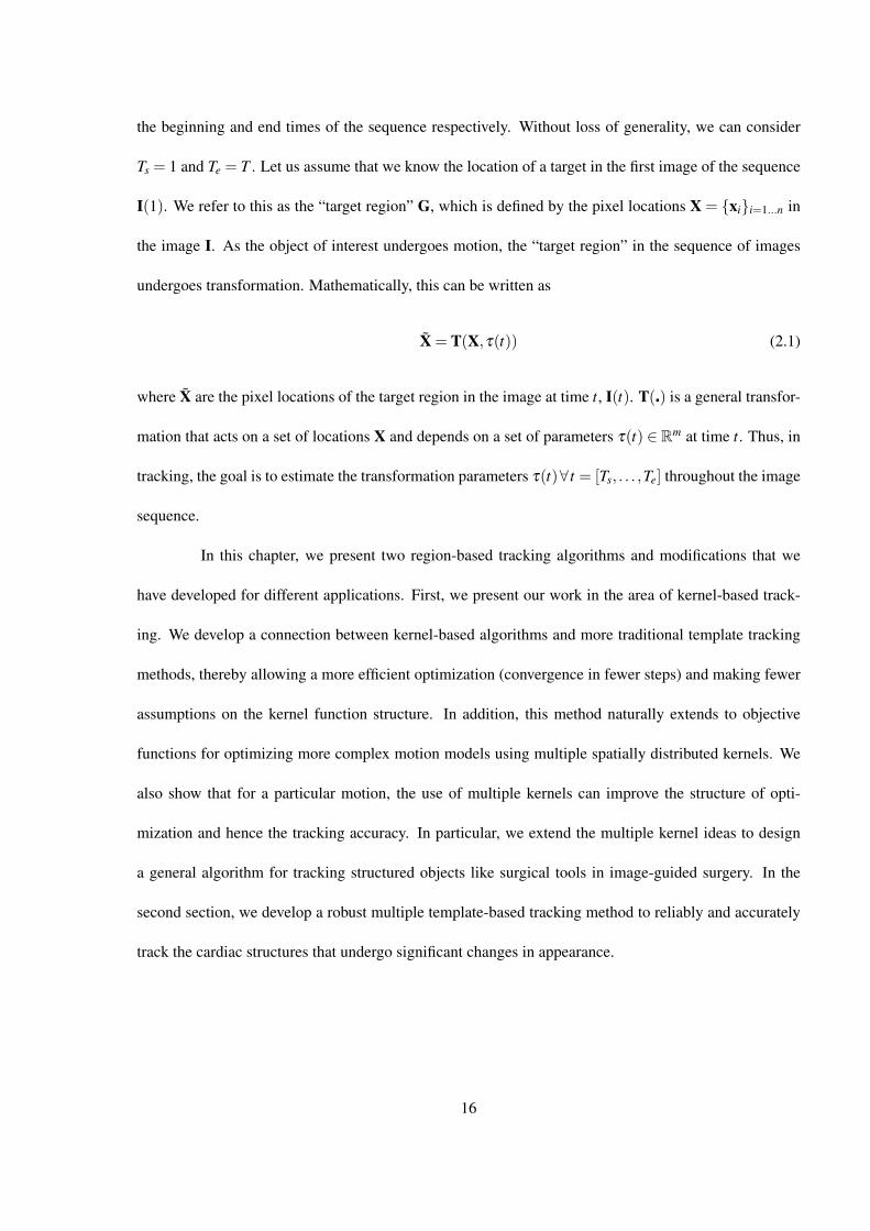
undergoes transformation. Mathematically, this can be written as

X = T(X,τ(t)) (2.1)

where X are the pixel locations of the target region in the image at time t, I(t). T(�) is a general transfor-

mation that acts on a set of locations X and depends on a set of parameters τ(t) ∈ Rm at time t. Thus, in

tracking, the goal is to estimate the transformation parameters τ(t)∀ t = [Ts, . . . ,Te] throughout the image

sequence.

In this chapter, we present two region-based tracking algorithms and modifications that we

have developed for different applications. First, we present our work in the area of kernel-based track-

ing. We develop a connection between kernel-based algorithms and more traditional template tracking

methods, thereby allowing a more efficient optimization (convergence in fewer steps) and making fewer

assumptions on the kernel function structure. In addition, this method naturally extends to objective

functions for optimizing more complex motion models using multiple spatially distributed kernels. We

also show that for a particular motion, the use of multiple kernels can improve the structure of opti-

mization and hence the tracking accuracy. In particular, we extend the multiple kernel ideas to design

a general algorithm for tracking structured objects like surgical tools in image-guided surgery. In the

second section, we develop a robust multiple template-based tracking method to reliably and accurately

track the cardiac structures that undergo significant changes in appearance.

16

2.1 Kernel-based Tracking

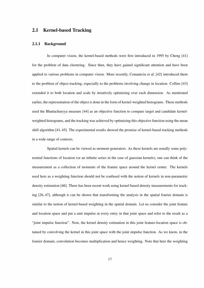
2.1.1 Background

In computer vision, the kernel-based methods were first introduced in 1995 by Cheng [41]

for the problem of data clustering. Since then, they have gained significant attention and have been

applied to various problems in computer vision. More recently, Comaniciu et al. [42] introduced them

to the problem of object tracking, especially to the problems involving change in location. Collins [43]

extended it to both location and scale by iteratively optimizing over each dimension. As mentioned

earlier, the representation of the object is done in the form of kernel-weighted histograms. These methods

used the Bhattacharyya measure [44] as an objective function to compare target and candidate kernel-

weighted histograms, and the tracking was achieved by optimizing this objective function using the mean

shift algorithm [41, 45]. The experimental results showed the promise of kernel-based tracking methods

in a wide range of contexts.

Spatial kernels can be viewed as moment-generators. As these kernels are usually some poly-

nomial functions of location (or an infinite series in the case of gaussian kernels), one can think of the

measurement as a collection of moments of the feature space around the kernel center. The kernels

used here as a weighting function should not be confused with the notion of kernels in non-parametric

density estimation [46]. There has been recent work using kernel based density measurements for track-

ing [26, 47], although it can be shown that transforming the analysis in the spatial fourier domain is

similar to the notion of kernel-based weighting in the spatial domain. Let us consider the joint feature

and location space and put a unit impulse at every entry in that joint space and refer to the result as a

“joint impulse function”. Now, the kernel density estimation in this joint feature-location space is ob-

tained by convolving the kernel in this joint space with the joint impulse function. As we know, in the

fourier domain, convolution becomes multiplication and hence weighting. Note that here the weighting

17

is done instead by the fourier transform of the kernel.

Intuitively, the attractiveness of the kernel-based descriptions of the tracking regions come

from the fact that they combine descriptions of both intensity values and spatial positions in a way that

avoids the need for complex modeling of object shape, appearance or motion. Thus, conceptually they

forge a link between statistical measures of similarity (which historically required brute force optimiza-

tion) with powerful methods from continuous optimization. The underlying assumption in kernel-based

tracking is that a statistical summary in terms of a kernel-weighted feature histogram is sufficient to de-

termine location, and is sufficiently insensitive to other motions to be robust. This raises a question as to

what motions can and cannot be recovered using kernel-based methods. For example, rotational motion

cannot be estimated with traditional kernel-based methods because only rotationally-symmetric kernels

have been used. On the other hand, most kernels are not scale-invariant, requiring some apparatus to deal

with scaling of the target.

In order to gain an understanding of the performance and performance limitations of tradi-

tional kernel-based methods, we propose to use a sum of squared differences (SSD) form of the original

Bhattacharyya metric. This allows for a Newton-style minimization procedure on this measure. The

structure of this optimization allows explicit study of the limitations in kernel-density tracking. These

limitations arise both from the structure of the kernel alone and from interactions between the kernel

and the image spatial structure. We also show empirically that the Newton-style formulation is a more

efficient optimization than mean shift which is fundamentally a gradient descent algorithm.

This analysis also provides a basis for considering the design of a set of kernel-based trackers

based on a particular tracking task. Intuitively, the use of multiple kernels increase the measurement

space and, should in theory increase the sensitivity of a kernel-based tracking algorithm. The SSD mea-

sure we develop extends naturally to multiple kernels. We show designs for kernels that are tailored to

particular types of image motions, including scale and rotation, and to particular types of image intensity

18

structures, including generic region properties such as symmetry.

2.1.2 Mean-shift formulation

In this section, we first re-derive the mean-shift formulation of kernel-based tracking [42, 25].

Let us consider again the target region defined by pixel locations {xi}i=1...n in an image I(t) with time

index t. For each pixel location, there is a feature vector f ∈F that characterizes the appearance within

some neighborhood of that pixel location. Let U = 1 . . .m represent a finite number of feature “bins,”

and let b : F →U denote the “binning” function on features. For simplicity, the expression b(x, t) will

represent the bin of the feature value of location x in an image with time index t. Let K : ℜ2 → ℜ+

denote a kernel which assigns weights to image locations. The argument to the kernel is usually a

normalized pixel coordinate x = x−ch , where c and h are the center location and scale of the kernel

function respectively. Here, c and h can be thought of as the transformation parameters τ as mentioned

in 2.1. For the analysis in this section, only the location of the kernel center c undergoes change and the

kernel scale h stays fixed.

With these definitions, a kernel-weighted empirical distribution, or histogram, q = (q1,q2, . . . ,qm)t of a

target region can be computed as:

qu = Cn

∑i=1

K(xi)δ (b(xi, t),u) (2.2)

C =1

∑ni=1 K(xi)

(2.3)

where δ is the Kronecker delta function. Note that the definition of C implies that ∑mu=1 qu = 1. Unless

otherwise noted, we subsequently consider only kernels that have been suitably normalized so that C = 1.

Equation (2.2) can be written more compactly by defining, for each feature value u, a corre-

sponding sifting vector u as ui = ui(t) = δ (b(xi, t),u). We can combine these sifting vectors into an n by

m sifting matrix U = [u1,u2, . . . ,um]. Similarly, we can define a vector version of the kernel function K

19

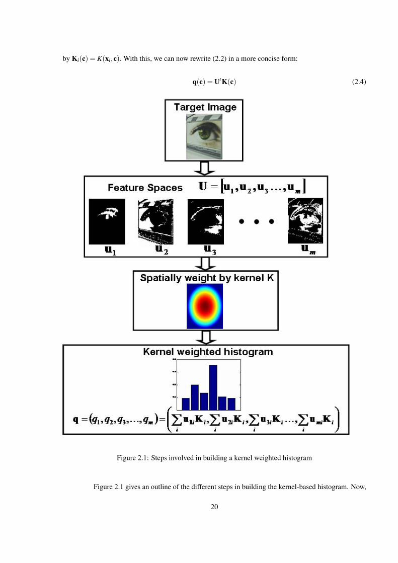
by Ki(c) = K(xi,c). With this, we can now rewrite (2.2) in a more concise form:

q(c) = UtK(c) (2.4)

Figure 2.1: Steps involved in building a kernel weighted histogram

Figure 2.1 gives an outline of the different steps in building the kernel-based histogram. Now,

20

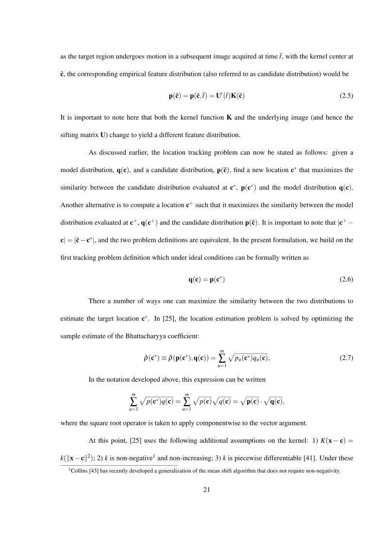
as the target region undergoes motion in a subsequent image acquired at time t, with the kernel center at

c, the corresponding empirical feature distribution (also referred to as candidate distribution) would be

p(c) = p(c, t) = Ut(t)K(c) (2.5)

It is important to note here that both the kernel function K and the underlying image (and hence the

sifting matrix U) change to yield a different feature distribution.

As discussed earlier, the location tracking problem can now be stated as follows: given a

model distribution, q(c), and a candidate distribution, p(c), find a new location c∗ that maximizes the

similarity between the candidate distribution evaluated at c∗, p(c∗) and the model distribution q(c).

Another alternative is to compute a location c+ such that it maximizes the similarity between the model

distribution evaluated at c+, q(c+) and the candidate distribution p(c). It is important to note that |c+−

c|= |c− c∗|, and the two problem definitions are equivalent. In the present formulation, we build on the

first tracking problem definition which under ideal conditions can be formally written as

q(c) = p(c∗) (2.6)

There a number of ways one can maximize the similarity between the two distributions to

estimate the target location c∗. In [25], the location estimation problem is solved by optimizing the

sample estimate of the Bhattacharyya coefficient:

ρ(c∗)≡ ρ(p(c∗),q(c)) =m

∑u=1

√pu(c∗)qu(c), (2.7)

In the notation developed above, this expression can be written

m

∑u=1

√p(c∗)q(c) =

m

∑u=1

√p(c)

√q(c) =

√p(c) ·

√q(c),

where the square root operator is taken to apply componentwise to the vector argument.

At this point, [25] uses the following additional assumptions on the kernel: 1) K(x− c) =

k(‖x− c‖2); 2) k is non-negative1 and non-increasing; 3) k is piecewise differentiable [41]. Under these1Collins [43] has recently developed a generalization of the mean shift algorithm that does not require non-negativity.

21

assumptions, the mean shift algorithm is then derived in two steps. The first step is to expand the above

expression in a Taylor series about p(c).

ρ(p(c∗),q(c)) = ρ(p(c),q(c))+∂ ρ(p(c∗),q(c))

∂p(c∗)

∣∣∣∣c∗=c

(p(c∗)−p(c))

=m

∑u=1

(√pu(c)qu(c))+

12

√qu(c)pu(c)

(pu(c∗)− pu(c))

)

=12

m

∑u=1

(√pu(c)qu(c)+

√qu(c)pu(c)

pu(c∗)

) (2.8)

As the first term in the last equation in (2.8) is a constant, the optimization involves maximizing

the last term only. Substituting the equation for the candidate distribution from equation (2.2), we obtain

the following objective function that needs to be maximized.

O(c∗) =n

∑i=1

wiK(xi− c∗) (2.9)

wi =m

∑u=1

√qu(c)√pu(c)

δ (b(xi, t),u) (2.10)

In the vector notation developed above, this becomes

w = U

(√q(c)√p(c)

)(2.11)

O(c∗) = wtK(c∗) (2.12)

where / is again taken to apply componentwise to the associated vectors.

The optimization problem is then solved by computing the gradient of O(c∗) and setting it

equal to zero [25]. The final solution takes the form of a weighted mean:

c∗− c =4c = ∑ni=1(xi− c)wig(‖xi− c‖2)

∑ni=1 wig(‖xi− c‖2)

(2.13)

where g(x) =−k′(x) and is known as the shadow kernel.

It can be shown that the series of “mean shifts” computed using this rule seeks the mode of the

kernel-weighted distribution of wi as a function of kernel location.

22

2.1.3 SSD Formulation

Now let us consider an alternative measure to maximize similarity between the model and

candidate distributions. The objective function is based on the sum of squared differences (SSD) between

the two distributions also known as the Matusita metric [48]

OM(c∗) = ‖√

q(c)−√

p(c∗)‖2. (2.14)

It is well known that the Matusita metric and the Bhattacharyya coefficient in 2.7 are related [48, 44] by

O(c∗) = 2−2ρ(c∗) (2.15)

As a result, the minima of (2.14) coincide with the maxima of the Bhattacharyya coefficient (2.7), and

hence we can equivalently work with (2.14), which we will refer to subsequently as the SSD error.

We derive a Newton-style iterative procedure to solve this optimization by expanding the ex-

pression for√

p(c∗) about c using Taylor series expansion and dropping higher order terms:

√p(c∗) =

√p(c)+

12

d(p(c))−12 UtJK(c)(c∗− c) (2.16)

where JK is the n by 2 matrix of the form

JK =[

∂K∂ c1

,∂K∂ c2

]=

∂K(x1−c)∂ c

∂K(x2−c)∂ c

...

∂K(xn−c)∂ c

and d(p) denotes the matrix with elements of p on its diagonal.

Thus the objective function in 2.14 can now be written in terms of a correction 4c = c∗− c as

O(4c) = ‖√

q(c)−√

p(c)− 12

d(p)−12 UtJK4c‖2 (2.17)

23

Now, provided that the kernel jacobian JU = d(p)−12 UtJK is of column rank 2, the minimum of the

objective function 2.17 is the solution of the following linear system

JtKUd(p)−1UtJK4c = 2Jt

KUd(p)−12

(√q(c)−

√p(c)

)(2.18)

The linear system optimization in (2.18) attempts to jump directly to the solution in a single step. Figure

2.2 shows a simple example of a return map2 illustrating this behavior. As with all gradient descent

algorithms, the mean shift algorithm presented in the previous section (see section 2.1.2) tends to under

perform the Newton style iteration procedure presented here.

2.1.4 More Complex Motion Models

The basic idea of kernel-based estimation can now be easily extended to recover richer models

of target motion following the line of development generally used for template tracking [4, 5]. Let

f (x,τ) represent a parametric deformation model of a target region characterized by the parameters

τ = (τ1,τ2, . . . ,τr). The function f is assumed to be differentiable w.r.t to both τ and x. The definition of

the kernel function can be extended to include f by defining

K(x,τ) = Cτ K( f (x,τ)) (2.19)

Cτ =1

∑i K( f (x,τ))(2.20)

Note we have been forced to reintroduce Cτ as non-rigid mappings f may change the effective area

under the kernel and thus the kernel will require renormalization. Also, note that the center location of the

kernel c is part of the parameters τ . Thus, from now on we will write K(x,τ) = K(x,(c, τ)) = K(x−c, τ).

With this, the definition of a corresponding vector form K(c, τ) exactly parallels the development above,

and thus we can now define a kernel-modulated histogram as:

q(c, τ) = UtK(c, τ) (2.21)2A return map is a plot showing the relationship between the estimated and true shift of a signal for a particular estimator.

24

−10 −5 0 5 10−6

−4

−2

0

2

4

6

8

shift in the rect signal (pixels)

corr

ecti

on a

fter

fir

st it

erat

ion

(pix

el)

mean shift (epan kernel)kernel−based SSD (epan kernel)kernel−based SSD (roof kernel)

−10 −5 0 5 10−15

−10

−5

0

5

10

15

shift in the step signal (pixels)

corr

ecti

on a

fter

fir

st it

erat

ion

(pix

els)

mean shift (epan kernel)kernel−based SSD (epan kernel)kernel−based SSD (roof kernel)

Figure 2.2: Return map comparison between mean shift and kernel-based SSD approach. The left plotcompares the return map for shift when the target is centered on “box” signal; the right plot the perfor-mance when the target is centered on a 1D step function (an “edge”). For kernel-based SSD approach,both epan and triangular kernels [46] have been used. It can be seen that SSD has nearly perfect 1-stepperformance, whereas mean shift much slower to return.

25

Again, following the same steps of Taylor series expansion, we see the histogram Jacobian

includes a kernel Jacobian that is now an n by r matrix of the general form:

JK =[

∂K∂c1

,∂K∂c2

,∂K∂ τ1

,∂K∂ τ2

, . . . ,∂K

∂ τr−2

]For a concrete example, consider the problem of determining the appropriate scaling of the

kernel as discussed in [43]. The three parameters of interest are the two translation parameters (cx,cy)

and one scaling parameter s. It is easy to show that for kernels with C = 1, the kernel Jacobian has the

general form

JK =

Kx,Ky,(xx− cx).∗Kx +(xy− cy).∗Ky− ((xx− cx).∗Kx +(xy− cy).∗Ky)K︸ ︷︷ ︸KS

where Kx = ∂K

∂c1, Ky = ∂K

∂c2, KS = ∂K

∂ s , (·) denotes the sum of the elements of the vector argument, and

.∗ denotes an element wise vector multiplication. The subtraction of the summed derivatives is a direct

consequence of the requirement that the kernel remain normalized after scaling. Now, if we add rotation

θ as well as a parameter, the kernel jacobian form becomes

JK = [Kx,Ky,KS,(xx− cx).∗Kx +(xy− cy).∗Ky− ((xx− cx).∗Kx +(xy− cy).∗Ky)K︸ ︷︷ ︸Kθ

where Kθ = ∂K∂θ

.

Given a predicted set of model parameters c and τ, a correction term (4c,4τ is computed as

the solution of the following linear system

JtKUd(p)−1UtJK

4c

4τ

= JtKUd(p)−

12 e (2.22)

e =√

q−√

p(c, τ) (2.23)

The general form and structure of f and the parameters τ has been discussed in-depth in [49] and would

like to refer the reader to it.

26

2.1.5 The Limits of Single Kernels

In this section we will discuss some of the properties of kernel-based tracking using a single

kernel. First, note that, as with the mean shift algorithm, histogram bins with zero values must be ignored

or otherwise regularized [50] in order for the inverse of d(p) to be well defined. Furthermore, the rank

of JU = d(p)−12 UtJK can in any case be no larger than min(r,m) [51], where r and m are the number of

transformation parameters and feature bins respectively. In fact, note that the mth value of the histogram

is a function of the previous m− 1 (due to the constraint that the histogram sums to 1), and it can be

easily shown that in the case of symmetric kernels this results in a rank reduction on UtJK. Additionally,

any zero values in the histogram will further lower m.

From this it follows that at least three different features values are necessary to track two de-

grees of translational freedom, no matter how the feature values are distributed. Moreover, this form

of rank deficiency is an inherent limitation on any kernel-based objective function. Alternatively, there

could be scenarios where there are local target motions that leave the value of the kernel-weighted his-

togram unchanged. This rank deficiency implies that these target motions lie in the kernel of JU.

Figure 2.3: A tracking on a bulls-eye figure.

To briefly illustrate these ideas, consider the image shown in Figure 2.3. The kernel at a is

27

ambiguous both because it only spans two colors, and because it lies along a spatial boundary i.e. motion

along this spatial boundary will go undetected. The kernel at b, although spanning three colors is still

invariant to the motion along the spatial boundary. Now, let us consider the kernel at c, centered on the

image. It can be worked out that the kernel-weighted histogram values are at an extremum here i.e. any

local motion would cause the histogram values corresponding to the gray and red color to decrease and

the value corresponding to the green color to increase. Additionally, interestingly enough, the circular

symmetry of the target matches the circular symmetry of the kernel causing the Jacobian JU to go to zero

indicating a complete breakdown of the derivative structure. Thus, not surprisingly, there is no single

kernel that can track this target over all sets of 2D translations.

Another possible way to have rank deficiency with an arbitrarily large number of feature values

is through appropriate interaction between the image and the kernel structure. In general, the invariance

of a kernel to a given motion is analytically equivalent to examining the equation

0 = Ut ∂K∂τ i

for parameter τ i of a given composition of kernel K and deformation f . If the chosen column vector

of partial derivatives of the kernel lies in the null space of the columns of U, then that deformation

is unrecoverable and JU will be rank deficient. This is the kernel-tracking equivalent of the aperture

problem. Additionally, other rank deficiencies can result due to linear combinations of local motions that

lie in the (column) null space of U.

2.1.6 Extension to Multiple Kernels

As discussed in the previous section, a single kernel, no matter what its structure, is ultimately

limited by two factors: 1) dimensionality of the histogram (which in turn may be a function of available

image structure), and 2) the interaction between its derivative structure and the spatial structure of the

image as it is exposed by the histogram. Thus, the obvious direction to pursue is to somehow increase

28

the dimensionality of the measurement space, and to simultaneously architect the derivative structure of

the kernel to be sensitive to desired directions of motion.

The recent paper by Collins [43] is in fact a step in this direction, where two kernels (one for

location and one for scale) are employed. We follow a similar approach by placing multiple kernels on

the image at locations (and ultimately profiles) that provide independent information on motion.

Consider the following roof kernel

Definition 1. A roof kernel of length l, span s, center c and normal vector n is defined as

Kr(x;c,n) =4

(l ∗ s2)max(s/2−|(x− c) ·n|,0).

Intuitively, a roof kernel is simply an extrusion of a triangular kernel. The choice of the roof

kernel above is motivated by the following observation. In 1-D, consider a triangular kernel centered

at a location where the signal changes histogram bins (and thus forms a step edge). In 1-D, the form

UtJK(x) computes the scalar convolution of the shadow kernel g (which is now itself a step edge) with

the underlying binned image at x. It follows that the triangular kernel, in the absence of noise, is the

optimal detector for the step edge in the binned signal when the center of the kernel c is at the step

edge [28]. Although this discussion is for the one-dimensional case, it is easy to see that a similar

argument can be made in for a two-dimensional roof kernel with orientation n, where n points along the

local “spatial gradient” of the binned image

Intuitively, two roof kernels oriented in orthogonal directions can provide independent infor-

mation on motion along the normal directions. Two such kernels in x and y direction are shown in Figure

2.4.

Algebraically, the use of two kernels doubles the dimension of the histogram, and therefore

increases the potential rank of the system. To formalize and generalize these ideas, we proceed as

follows:

29

Figure 2.4: The x and y roof kernels.

Suppose we adjoin several kernels into an n× r kernel matrix given as

K(α) = [K1(α1),K2(α2), . . . ,Kr(αr)]

where αi are the transformation parameters for the ith kernel Ki and α = (α1,α2, . . . ,αm), with some

constraints over the transformation parameters. The constraints arise as the transformation parameters αi

of these kernels can have similar or overlapping parameter coefficients αi j, where αi = (αi1,αi2, . . . ,αim).

For example, two kernels can have similar or different centers c.

Following the development earlier, we can now define matrices that contain the corresponding

model and target histograms as Q = U(t0)tK(α0) and P(α, t) = U(t)tK(α). Here, again α0 is known and

the goal is to compute the transformation parameters α . The optimization is then

O(α) = ‖Q−P(α, t)‖2 (2.24)

where ‖ · ‖ now denotes the Frobenius norm.

At this point, it is useful to recall that the Frobenius norm on a matrix is equivalent to the

norm of the single column vector constructed by concatenating the columns of the matrix. Let p and q

denote the “stacked” versions of P and Q. By recasting the problem in this form, and performing the

30

same Taylor series expansion, we have:

e =√

p(α, t)−√

q (2.25)

JU(τ) = d(p)−12

UtJK(α1)

...

UtJK(αr)

(2.26)

JtUJU4α = Jt

Ue (2.27)

It is important to note that the algebraic structure of the stacked system can be no worse than

that of any single kernel, and in general will be much better. This does not imply though that multiple

kernels will lead to an improvement in the tracking accuracy/quality. Thus, care and analysis of kernel

properties is essential in constructing multi-kernel trackers.

2.1.7 The Relationship Between Spatial Structure and Kernel Structure

Consider a binned image B(x) = b(I(x)) undergoing deformations f . Let x1,x2, . . .xs denote s

image locations in the binned image with local gradient directions gi = (dxi,dyi) i = 1 . . .s. Define

JI =

∂ I( f (x;τ))/∂τ∣∣x1,τ=0

∂ I( f (x;τ))/∂τ∣∣x2,τ=0

...

∂ I( f (x;τ))/∂τ∣∣xs,τ=0

and

JK =

∂K( f (x;τ),c1)/∂τ∣∣x1,τ=0

∂K( f (x;τ),c1)/∂τ∣∣x2,τ=0

...

∂K( f (x;τ),c1)/∂τ∣∣xs,τ=0

31

Now, we know maximum rank of Ut and JK is m and r respectively. Here m is the number of

feature bins and r is the number of transformation parameters i.e. length of the τ vector. We know from

matrix algebra [51] that for two multiplicative matrices A and B, rank(AB) ≤ min(rank(A),rank(B))

i.e. matrix multiplication can lead to a rank reduction. Additionally, as discussed in Section 2.1.5,

we know m is usually greater than r. Therefore, rank(UtJK) ≤ r. In general, rank(JI) = r, therefore

rank(JI)≥ rank(UtJK). This analysis is with a single kernel K.

Now, if we use multiple kernels, it is easy to see that one reverse the equation such that

rank(UtJK)≥ rank(JI). This shows more formally that we can increase the rank structure of the tracking

problem through the use of multiple kernels.

2.1.8 Multiple Kernel Constructions

In the previous section, we already motivated one possible multi-kernel construction: the com-

bination of two roof kernels in orthogonal directions to provide location information. In particular, if we

return to the simple bulls-eye example in Figure 2.5, it is easy to see that the two x and y directional

ramp kernels can now provide two independent measures of x and y translation motion, and thus it is

possible to track the target undergoing 2D translation. It is important to note that we still have invari-

ance to rotation, although a kernel that is not centered on the perimeter of the red circle can be added to

compute rotation in an implicit manner.

Once we take the step of allowing multiple kernels, there are a number additional possibilities

for defining tracking structures. Here we detail a few.

Symmetry Seeking: As currently defined, the goal of kernel-based tracking is to match a fixed kernel-

weighted histogram to a time and parameter varying one. An alternative is to match two time and location

varying histograms to each other. This is particularly useful in cases where the image itself exhibits some

type of symmetry, in which case the trackers will be forced into a symmetric configuration. For example,

32

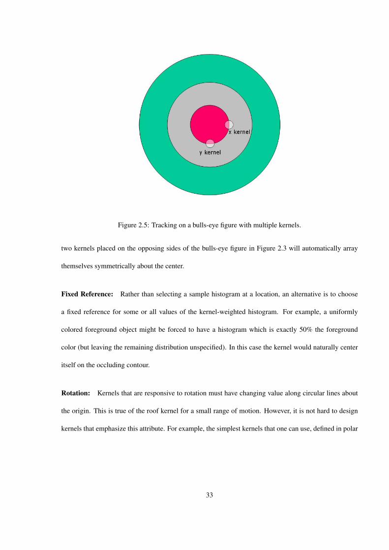
Figure 2.5: Tracking on a bulls-eye figure with multiple kernels.

two kernels placed on the opposing sides of the bulls-eye figure in Figure 2.3 will automatically array

themselves symmetrically about the center.

Fixed Reference: Rather than selecting a sample histogram at a location, an alternative is to choose

a fixed reference for some or all values of the kernel-weighted histogram. For example, a uniformly

colored foreground object might be forced to have a histogram which is exactly 50% the foreground

color (but leaving the remaining distribution unspecified). In this case the kernel would naturally center

itself on the occluding contour.

Rotation: Kernels that are responsive to rotation must have changing value along circular lines about

the origin. This is true of the roof kernel for a small range of motion. However, it is not hard to design

kernels that emphasize this attribute. For example, the simplest kernels that one can use, defined in polar

33

coordinates (θ ,r) are

K1(θ ,r) = θ2

K2(θ ,r) = sin2(θ)

(2.28)

where θ is the angle from the center of the kernel and r < rmax. Figure 2.6 shows these kernels. Both

these kernels have discontinuities and high values at the boundaries, which are undesirable properties.

The use of the following kernel overcomes these limitations.

K(θ ,r) = r2(rmax− r2)sin2(m∗θ) (2.29)

where m ∈R. Two of these kernels with different values of m are shown in the bottom row of Figure 2.6.

Note that m controls the number of lobes in the kernel.

Figure 2.6: Different rotation kernels. The top row shows the kernels in (2.28) and the bottom row showsthe kernels in (2.29).

34

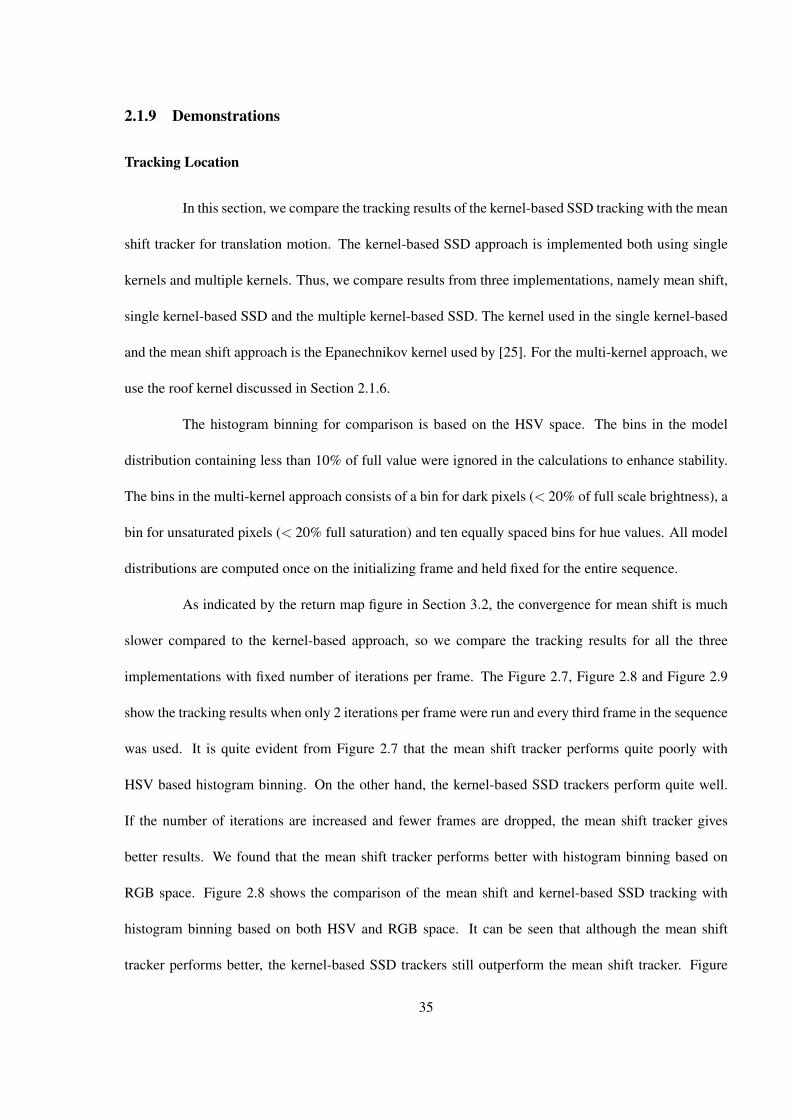
2.1.9 Demonstrations

Tracking Location

In this section, we compare the tracking results of the kernel-based SSD tracking with the mean

shift tracker for translation motion. The kernel-based SSD approach is implemented both using single

kernels and multiple kernels. Thus, we compare results from three implementations, namely mean shift,

single kernel-based SSD and the multiple kernel-based SSD. The kernel used in the single kernel-based

and the mean shift approach is the Epanechnikov kernel used by [25]. For the multi-kernel approach, we

use the roof kernel discussed in Section 2.1.6.

The histogram binning for comparison is based on the HSV space. The bins in the model

distribution containing less than 10% of full value were ignored in the calculations to enhance stability.

The bins in the multi-kernel approach consists of a bin for dark pixels (< 20% of full scale brightness), a

bin for unsaturated pixels (< 20% full saturation) and ten equally spaced bins for hue values. All model

distributions are computed once on the initializing frame and held fixed for the entire sequence.

As indicated by the return map figure in Section 3.2, the convergence for mean shift is much

slower compared to the kernel-based approach, so we compare the tracking results for all the three

implementations with fixed number of iterations per frame. The Figure 2.7, Figure 2.8 and Figure 2.9

show the tracking results when only 2 iterations per frame were run and every third frame in the sequence

was used. It is quite evident from Figure 2.7 that the mean shift tracker performs quite poorly with

HSV based histogram binning. On the other hand, the kernel-based SSD trackers perform quite well.

If the number of iterations are increased and fewer frames are dropped, the mean shift tracker gives

better results. We found that the mean shift tracker performs better with histogram binning based on

RGB space. Figure 2.8 shows the comparison of the mean shift and kernel-based SSD tracking with

histogram binning based on both HSV and RGB space. It can be seen that although the mean shift

tracker performs better, the kernel-based SSD trackers still outperform the mean shift tracker. Figure

35

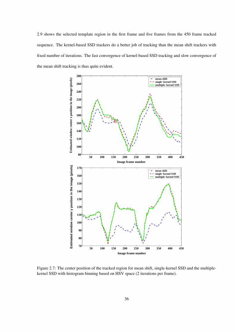
2.9 shows the selected template region in the first frame and five frames from the 450 frame tracked

sequence. The kernel-based SSD trackers do a better job of tracking than the mean shift trackers with

fixed number of iterations. The fast convergence of kernel-based SSD tracking and slow convergence of

the mean shift tracking is thus quite evident.

50 100 150 200 250 300 350 400 45080

100

120

140

160

180

200

220

240

260

280

Image frame number

Est

imat

ed w

indo

w c

ente

r x

posi

tion

in t

he im

age

(pix

els) mean shift

single−kernel SSDmultiple−kernel SSD

50 100 150 200 250 300 350 400 45070

80

90

100

110

120

130

140

150

160

170

Image frame number

Est

imat

ed w

ind

ow

cen

ter

y p

osi

tio

n in

th

e im

age

(pix

els)

mean shiftsingle−kernel SSDmultiple−kernel SSD

Figure 2.7: The center position of the tracked region for mean shift, single-kernel SSD and the multiple-kernel SSD with histogram binning based on HSV space (2 iterations per frame).

36

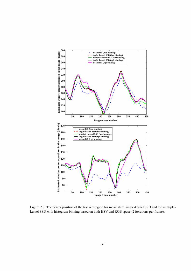
50 100 150 200 250 300 350 400 450

100

120

140

160

180

200

220

240

260

280

300

Image frame number

Est

imat

ed w

indo

w c

ente

r x

posi

tion

in t

he im

age

(pix

els) mean shift (hue binning)

single−kernel SSD (hue binning)multiple−kernel SSD (hue binning)single−kernel SSD (rgb binning)mean shift (rgb binning)

50 100 150 200 250 300 350 400 450

80

90

100

110

120

130

140

150

160

170

Image frame number

Est

imat

ed w

ind

ow

cen

ter

y p

osi

tio

n in

th

e im

age

(pix

els)

mean shift (hue binning)single−kernel SSD (hue binning)multiple−kernel SSD (hue binning)single−kernel SSD (rgb binning)mean shift (rgb binning)

Figure 2.8: The center position of the tracked region for mean shift, single-kernel SSD and the multiple-kernel SSD with histogram binning based on both HSV and RGB space (2 iterations per frame).

37

Figure 2.9: Tracking comparison for mean shift, single-kernel SSD and multiple-kernel SSD approacheswith 2 iterations per frame. The first frame shows the selected template region. In the following frames(frame numbers 98, 158, 290, 332, and 413) the tracked region from these different tracking approachesare shown. The tracked region in each frame for mean shift, single-kernel SSD and multiple-kernel SSDwith histogram binning based on HSV space are shown in blue, red and green rectangle respectively.The tracked region with histogram binning based on RGB space for mean shift and single-kernel SSDare shown in magenta and black respectively.

38

Tracking Similarities

As discussed earlier in the Section 2.1.6, the power of the multiple-kernel SSD tracking lies in

tracking similarities. Different kernels for each similarity namely x translation, y translation, scale and

rotation can be used to compute each of these similarities. In Figure 2.10, we show results for tracking

an image sequence with primarily translation and scale. Two orthogonal triangular kernels are used for

x and y translation and a limited conical kernel is used for scaling. Six frames from a 90 frame sequence

are shown. It can be easily seen the scaling changes by more than a factor of 2. Similarly, Figure

2.11 shows the tracking under translation, scale and rotation. The rotational kernel used is the one

defined in equation 2.29. Note that, as scale and rotation effects are nonlinear, and the optimization uses

linearization, tracking under large changes of both tend to make the tracking unstable.

2.1.10 Structured Tracking Example - Tool Tracking for Image-guided Retinal

Surgery

As discussed in Chapter 1, the guidance of the image-guided robot-assisted surgical proce-

dures can be enhanced by dynamically reconstructing the surgical environment. This involves tracking

surgical tools, devices and other features. In this section, we present an algorithm that we have developed

specifically for the task of tool tracking in our vision-based virtual fixture implementation to simulate the

basic concepts in retinal surgery. More details regarding the experimental setup can be found in [23,24].

We wish to note that, although developed for a specific application, the underlying idea is generic and

can be easily extended for tracking other structured objects. The challenges involved in tool tracking are

primarily due to the thin tool structure. Owing to the thin structure of the tool and changing background

structure around it, the conventional region-based tracking methods [4, 5] cannot be used for estimating

tool motion as the motion from the moving background will also be picked up. Therefore, one natural

way to track would be to first segment the tool to remove the background, and then estimate the tool

39

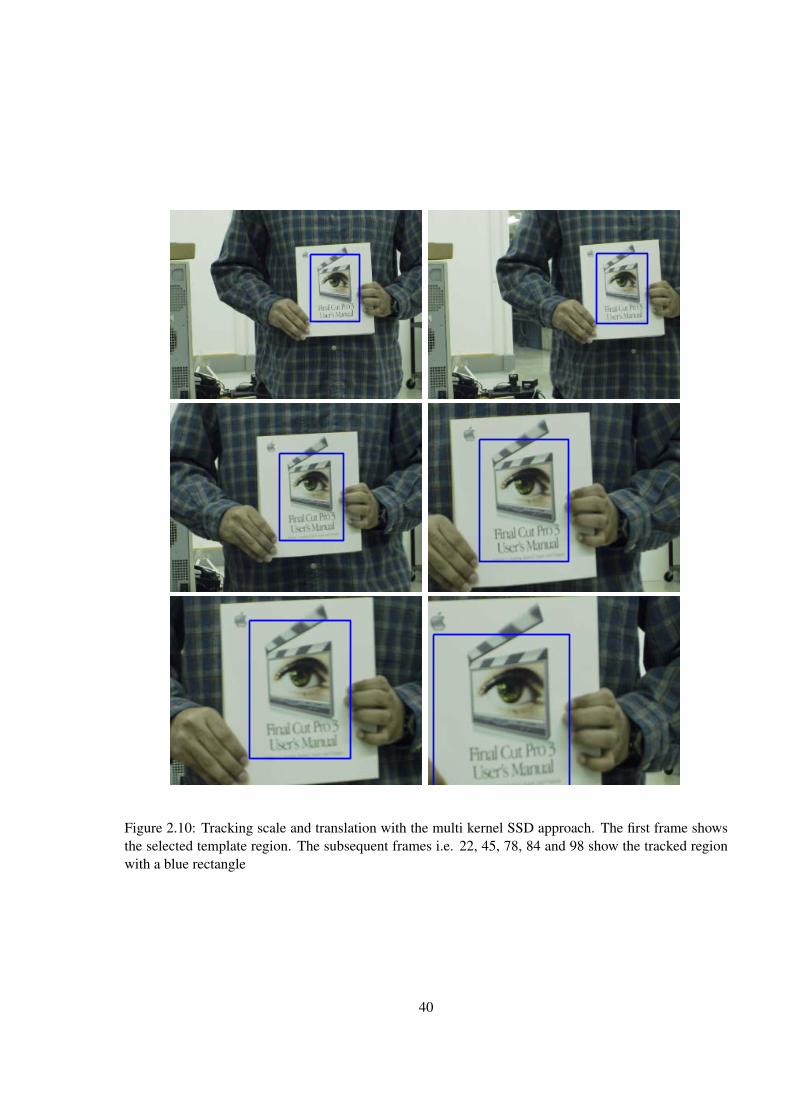
Figure 2.10: Tracking scale and translation with the multi kernel SSD approach. The first frame showsthe selected template region. The subsequent frames i.e. 22, 45, 78, 84 and 98 show the tracked regionwith a blue rectangle

40

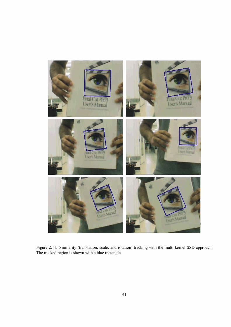
Figure 2.11: Similarity (translation, scale, and rotation) tracking with the multi kernel SSD approach.The tracked region is shown with a blue rectangle

41

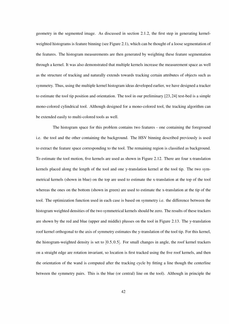
geometry in the segmented image. As discussed in section 2.1.2, the first step in generating kernel-

weighted histograms is feature binning (see Figure 2.1), which can be thought of a loose segmentation of

the features. The histogram measurements are then generated by weighting these feature segmentation

through a kernel. It was also demonstrated that multiple kernels increase the measurement space as well

as the structure of tracking and naturally extends towards tracking certain attributes of objects such as

symmetry. Thus, using the multiple kernel histogram ideas developed earlier, we have designed a tracker

to estimate the tool tip position and orientation. The tool in our preliminary [23, 24] test-bed is a simple

mono-colored cylindrical tool. Although designed for a mono-colored tool, the tracking algorithm can

be extended easily to multi-colored tools as well.

The histogram space for this problem contains two features - one containing the foreground

i.e. the tool and the other containing the background. The HSV binning described previously is used

to extract the feature space corresponding to the tool. The remaining region is classified as background.

To estimate the tool motion, five kernels are used as shown in Figure 2.12. There are four x-translation

kernels placed along the length of the tool and one y-translation kernel at the tool tip. The two sym-

metrical kernels (shown in blue) on the top are used to estimate the x-translation at the top of the tool

whereas the ones on the bottom (shown in green) are used to estimate the x-translation at the tip of the

tool. The optimization function used in each case is based on symmetry i.e. the difference between the

histogram weighted densities of the two symmetrical kernels should be zero. The results of these trackers

are shown by the red and blue (upper and middle) plusses on the tool in Figure 2.13. The y-translation

roof kernel orthogonal to the axis of symmetry estimates the y-translation of the tool tip. For this kernel,

the histogram-weighted density is set to [0.5,0.5]. For small changes in angle, the roof kernel trackers

on a straight edge are rotation invariant, so location is first tracked using the five roof kernels, and then

the orientation of the wand is computed after the tracking cycle by fitting a line though the centerline

between the symmetry pairs. This is the blue (or central) line on the tool). Although in principle the

42

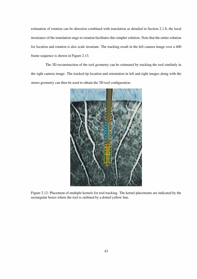
estimation of rotation can be direction combined with translation as detailed in Section 2.1.8, the local

invariance of the translation stage to rotation facilitates this simpler solution. Note that the entire solution

for location and rotation is also scale invariant. The tracking result in the left camera image over a 400

frame sequence is shown in Figure 2.13.

The 3D reconstruction of the tool geometry can be estimated by tracking the tool similarly in

the right camera image. The tracked tip location and orientation in left and right images along with the

stereo geometry can then be used to obtain the 3D tool configuration.

Figure 2.12: Placement of multiple kernels for tool tracking. The kernel placements are indicated by therectangular boxes where the tool is outlined by a dotted yellow line.

43

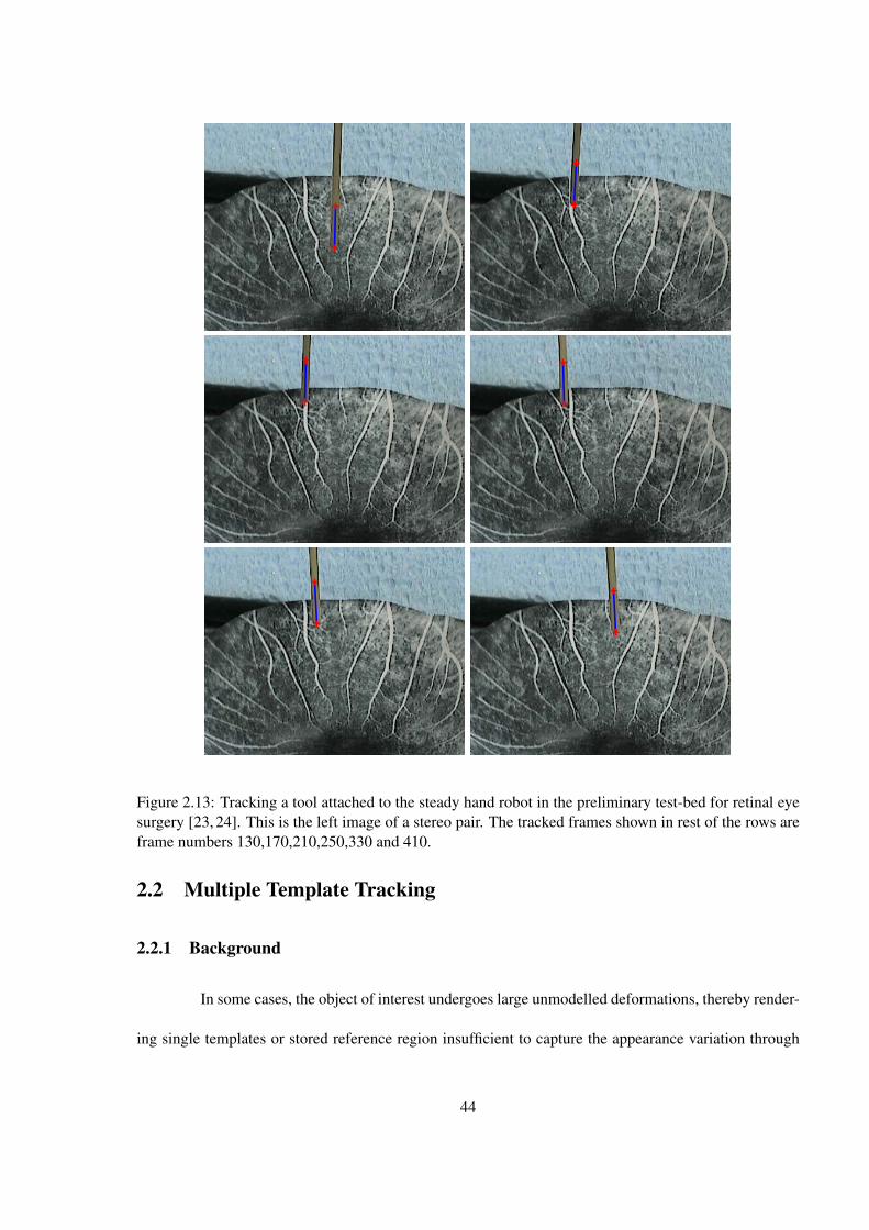
Figure 2.13: Tracking a tool attached to the steady hand robot in the preliminary test-bed for retinal eyesurgery [23, 24]. This is the left image of a stereo pair. The tracked frames shown in rest of the rows areframe numbers 130,170,210,250,330 and 410.

2.2 Multiple Template Tracking

2.2.1 Background

In some cases, the object of interest undergoes large unmodelled deformations, thereby render-

ing single templates or stored reference region insufficient to capture the appearance variation through

44

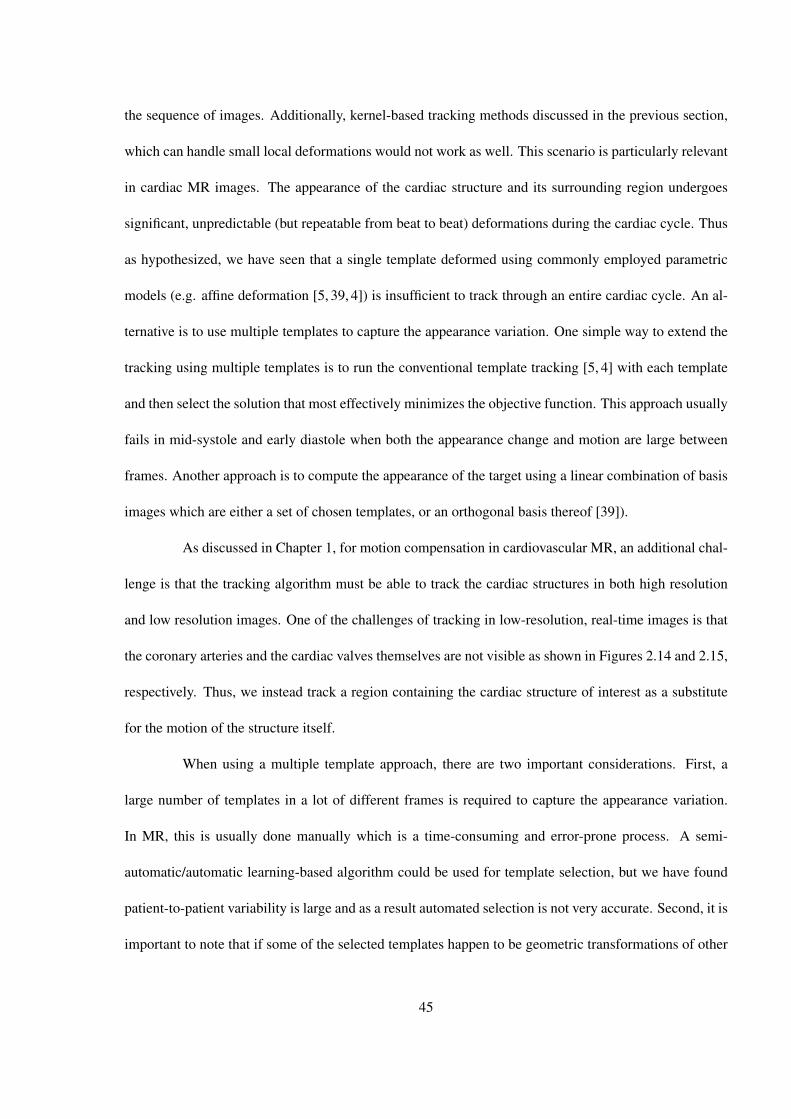
the sequence of images. Additionally, kernel-based tracking methods discussed in the previous section,

which can handle small local deformations would not work as well. This scenario is particularly relevant

in cardiac MR images. The appearance of the cardiac structure and its surrounding region undergoes

significant, unpredictable (but repeatable from beat to beat) deformations during the cardiac cycle. Thus

as hypothesized, we have seen that a single template deformed using commonly employed parametric

models (e.g. affine deformation [5, 39, 4]) is insufficient to track through an entire cardiac cycle. An al-

ternative is to use multiple templates to capture the appearance variation. One simple way to extend the

tracking using multiple templates is to run the conventional template tracking [5, 4] with each template

and then select the solution that most effectively minimizes the objective function. This approach usually

fails in mid-systole and early diastole when both the appearance change and motion are large between

frames. Another approach is to compute the appearance of the target using a linear combination of basis

images which are either a set of chosen templates, or an orthogonal basis thereof [39]).

As discussed in Chapter 1, for motion compensation in cardiovascular MR, an additional chal-

lenge is that the tracking algorithm must be able to track the cardiac structures in both high resolution

and low resolution images. One of the challenges of tracking in low-resolution, real-time images is that

the coronary arteries and the cardiac valves themselves are not visible as shown in Figures 2.14 and 2.15,

respectively. Thus, we instead track a region containing the cardiac structure of interest as a substitute

for the motion of the structure itself.

When using a multiple template approach, there are two important considerations. First, a

large number of templates in a lot of different frames is required to capture the appearance variation.

In MR, this is usually done manually which is a time-consuming and error-prone process. A semi-

automatic/automatic learning-based algorithm could be used for template selection, but we have found

patient-to-patient variability is large and as a result automated selection is not very accurate. Second, it is

important to note that if some of the selected templates happen to be geometric transformations of other

45

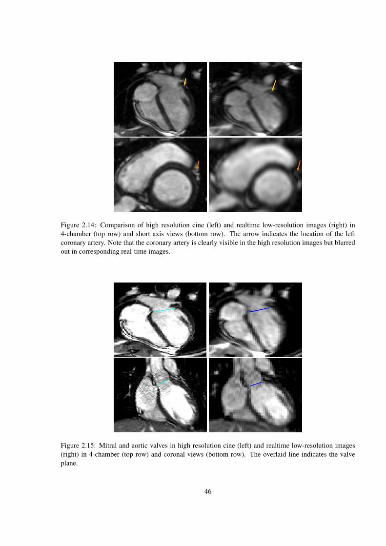
Figure 2.14: Comparison of high resolution cine (left) and realtime low-resolution images (right) in4-chamber (top row) and short axis views (bottom row). The arrow indicates the location of the leftcoronary artery. Note that the coronary artery is clearly visible in the high resolution images but blurredout in corresponding real-time images.

Figure 2.15: Mitral and aortic valves in high resolution cine (left) and realtime low-resolution images(right) in 4-chamber (top row) and coronal views (bottom row). The overlaid line indicates the valveplane.

46

selected templates, the algorithm can (and will) compensate for motion using appearance variation. As

a result, without careful choice of templates, multiple template tracking can significantly underestimate

motion. We return to this point in section 2.2.4.

Therefore, we present a new tracking framework that makes use of multiple templates but

avoids the shortcomings mentioned above. This method incorporates two novel features. First, we

derive a bi-directional, coordinate-descent optimization that simultaneously computes the location and

affine mixture in each image. Second, we present a semi-automated selection method for template selec-

tion, which ensures that independent templates are chosen from points where the target undergoes large

changes.

In the next few sections, we first formulate the multiple template problem as a constrained

optimization, and derive an initial solution. We then show that this solution can be extended to a bi-

directional coordinate descent algorithm. Finally, we present a method for template selection to ensure

reliable and accurate tracking.

2.2.2 Affine-weighted SSD formulation

Following [39, 4], the basic idea behind the tracking approach is to describe the current region

of interest or the target as a geometric transformation of an affine combination of a set of templates.

For expressing this in a mathematical setting, we use the notation and terminology defined earlier in the

chapter. Let Zi; i = 1...m be the reference templates or target regions selected from a given sequence of

images Ii; i = 1...m. We express the current target region in terms of the reference templates as

Gt = T (m

∑i=1

wiZi,τ) (2.30)

where wi is the weight corresponding to template Zi and τ are the transformation parameters. The trans-

formation T is an operator defined on the locations of the image region s.t. T (Zi,τ) = Zi(T (xi,τ)) ∀xi ∈

X. For example, for a simple translational motion model, one can write T (Zi,u) = Zi(xi + u) ∀xi ∈ X

47

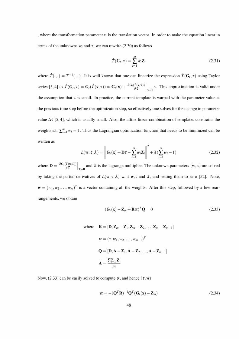
, where the transformation parameter u is the translation vector. In order to make the equation linear in

terms of the unknowns wi and τ , we can rewrite (2.30) as follows

T (Gt ,τ) =m

∑i=1

wiZi (2.31)

where T (., .) = T−1(., .). It is well known that one can linearize the expression T (Gt ,τ) using Taylor

series [5, 4] as T (Gt ,τ) = Gt(T (x,τ)) ≈ Gt(x)+ ∂Gt(T (x,τ))∂τ

∣∣∣τ=0

τ . This approximation is valid under

the assumption that τ is small. In practice, the current template is warped with the parameter value at

the previous time step before the optimization step, so effectively one solves for the change in parameter

value ∆τ [5, 4], which is usually small. Also, the affine linear combination of templates constrains the

weights s.t. ∑mi=1 wi = 1. Thus the Lagrangian optimization function that needs to be minimized can be

written as

L(w,τ,λ ) =

∥∥∥∥∥Gt(x)+Dτ−m

∑i=1

wiZi

∥∥∥∥∥2

+λ (m

∑i=1

wi−1) (2.32)

where D = ∂Gt(T (x,τ))∂τ

∣∣∣τ=0

and λ is the lagrange multiplier. The unknown parameters (w,τ) are solved

by taking the partial derivatives of L(w,τ,λ ) w.r.t w,τ and λ , and setting them to zero [52]. Note,

w = (w1,w2, . . . ,wm)T is a vector containing all the weights. After this step, followed by a few rear-

rangements, we obtain

(Gt(x)−Zm +Rα)T Q = 0 (2.33)

where R = [D,Zm−Z1,Zm−Z2, . . . ,Zm−Zm−1]

α = (τ,w1,w2, . . . ,wm−1)T

Q = [D,A−Z1,A−Z2, . . . ,A−Zm−1]

A = ∑mi=1 Zi

m

Now, (2.33) can be easily solved to compute α , and hence (τ,w)

α =−(QT R)−1QT (Gt(x)−Zm) (2.34)

48

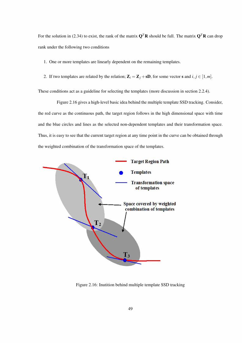
For the solution in (2.34) to exist, the rank of the matrix QT R should be full. The matrix QT R can drop

rank under the following two conditions

1. One or more templates are linearly dependent on the remaining templates.

2. If two templates are related by the relation; Zi = Z j + sD, for some vector s and i, j ∈ [1,m].

These conditions act as a guideline for selecting the templates (more discussion in section 2.2.4).

Figure 2.16 gives a high-level basic idea behind the multiple template SSD tracking. Consider,

the red curve as the continuous path, the target region follows in the high dimensional space with time

and the blue circles and lines as the selected non-dependent templates and their transformation space.

Thus, it is easy to see that the current target region at any time point in the curve can be obtained through

the weighted combination of the transformation space of the templates.

Figure 2.16: Inutition behind multiple template SSD tracking

49

2.2.3 Extension to Bidirectional Methods

It has been shown that bidirectional gradient methods [53,54] significantly improve the rate of

convergence and convergence range of the local optimization. Therefore, in this section, we extend the

multiple-template tracking described in section 2.2.2 to a bidirectional formulation. In order to do so,

equation 2.30, can be written symmetrically about τ as

T (Gt ,−τ/2) = T (m

∑i=1

wiZi,τ/2) (2.35)

Following the steps in section 2.2.2, the Lagrangian optimization function becomes

L(w,τ,λ ) =

∥∥∥∥∥∥∥∥∥Gt(x)−Dτ/2−m

∑i=1

wi(Zi +DZi︸ ︷︷ ︸P

)

∥∥∥∥∥∥∥∥∥2

+λ (m

∑i=1

wi−1)

(2.36)

where D = ∂Gt(T (x,τ))∂τ

∣∣∣τ=0

and DZi = ∂Zi(T (x,τ))∂τ

∣∣∣τ=0

. Taking partial derivatives of L(w,τ,λ ) w.r.t. w,τ

and λ , and eliminating λ , one gets the partial derivatives w.r.t. wi’s and τ as follows

∂L∂wi

= PT[M− (Zi +DZi

τ

2)]

, i = 1, ...,m−1 (2.37a)

∂L∂τ

= PT

[−D

2−

m

∑i=1

wiDZi

](2.37b)

where M = ∑mi=1 Zi+DZiτ/2

m and P is the given by underbrace in 2.36. It can be noted that the partial

derivative w.r.t. wm is not required as it is linearly dependent on the other m−1 partial derivatives w.r.t.

wi, i = 1, ...,m− 1. Since the partial derivatives in 2.37 are non-linear in wi’s and τ , the optimization

cannot be solved in closed form. Another way of solving the optimization is by iteratively solving each

subequation in 2.37 separately by keeping the other variable constant, also known as coordinate descent

algorithm [52]. If the other variable is kept constant, the solution now becomes

(w1, . . . ,wm−1)T = (Q1T R1)−1Q1T E1 (2.38a)

τ = (JT J)−1JT (Gt −m

∑i=1

wiZi) (2.38b)

50

where E1 = Gt −τ

2D− (Zm +

τ

2DZm)

J =D+∑

mi=1 DZi

2

and the ith column of R1 and Q1 are given by

[R1i] =[Zi−Zm +

τ

2(DZi−DZm)

][Q1i] =

[M− (Zi +

τ

2DZi)

]One of the limitations of the coordinate descent algorithm is that it can get stuck in local minima if not

properly initialized. We initialize the algorithm with the τ value obtained from 2.34 which is usually a

good initialization.

2.2.4 Template Selection

In order to make sure the solution in 2.34 and 2.38 is non-singular, the following matrix should

be well conditioned

N = [Z1,DZ1,Z2,DZ2, . . . ,Zm,DZm] (2.39)

where DZi = ∂Zi(T (x,τ))∂τ

∣∣∣τ=0

. A large condition number indicates a poor selection of templates indi-

cating that a template is a transformation of some other template or a combination of templates. For

the matrix QT R, this can also happen when the target region in the current frame is close to one of the

two templates. An assumption made here is that the derivative of the current region D will be close to

the linear combination of the derivative of templates. Although, the matrix N indicates whether a given

set of templates would ensure a non-singular solution of the optimization but it does not tell you which

templates to select from a given set of templates.

If we take a closer look at the matrix N, the two columns [Zi,DZi] corresponding to a template

Zi constitute the transformation tangent plane [55] of the template Zi. It is easy to see that if the tangent

51

planes of the selected templates that constitute the matrix N are well separated, the matrix N will be well-

conditioned. This notion can be captured by “tangent distance” [55], that is defined as the minimum

distance between the two tangent planes. Thus, to ensure a non-singular solution, one needs to find

a set of templates with well separated tangent planes and are a representative set of all the templates.

Hence, our algorithm is based on clustering using the tangent distance. We use the spectral clustering

method proposed by Ng et. al. [56]. Each entry in the affinity matrix is the tangent distance between the

two corresponding templates. The number of clusters is chosen by the user from the eigenvalues of the

normalized eigenvector matrix generated from the affinity matrix. The templates that are closest to the

cluster mean centers are selected for tracking.

In order to test the algorithm, we ran it on manually selected templates chosen at the left end

of the mitral valve in the 4-chamber view. In this case, the number of clusters was chosen to be 3, as the

first three eigenvalues of the normalized eigenvector matrix were most significant. Figure 2.17 shows the

optimal templates selected at frames 5, 17 and 36. The tracking was performed using these templates.

To compare it with a non-optimal choice of templates, the tracking was also run with equally spaced

templates at frames (5,20,35) and (1,20,40) respectively. The tracking results are compared in Figure

2.18. The tracking result for optimal templates was found to be visually the best. It is important to note

that the manual selection is not ground truth as it is very difficult to select templates with continuous

motion. The tracking results for “equal-spaced 1” and optimal templates are close as the templates lie in

similar clusters. Another point to note is that in the current formulation, we pick the template closest to

the mean as the optimal template in that cluster which might not be the best template corresponding to

that cluster. Also, increasing the number of optimal templates can further improve the tracking. Further

analysis regarding optimal templates can be found in Section 5.4.1.

52

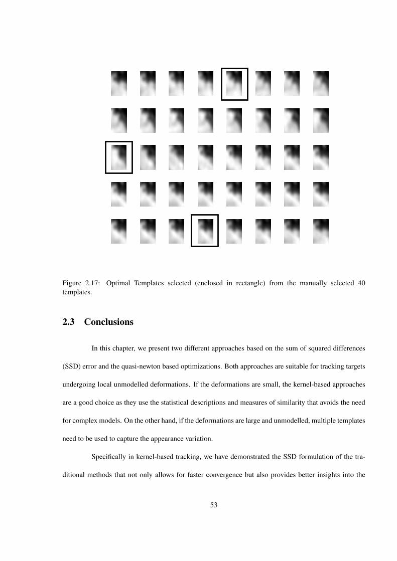
Figure 2.17: Optimal Templates selected (enclosed in rectangle) from the manually selected 40templates.

2.3 Conclusions

In this chapter, we present two different approaches based on the sum of squared differences

(SSD) error and the quasi-newton based optimizations. Both approaches are suitable for tracking targets

undergoing local unmodelled deformations. If the deformations are small, the kernel-based approaches

are a good choice as they use the statistical descriptions and measures of similarity that avoids the need

for complex models. On the other hand, if the deformations are large and unmodelled, multiple templates

need to be used to capture the appearance variation.

Specifically in kernel-based tracking, we have demonstrated the SSD formulation of the tra-

ditional methods that not only allows for faster convergence but also provides better insights into the

53

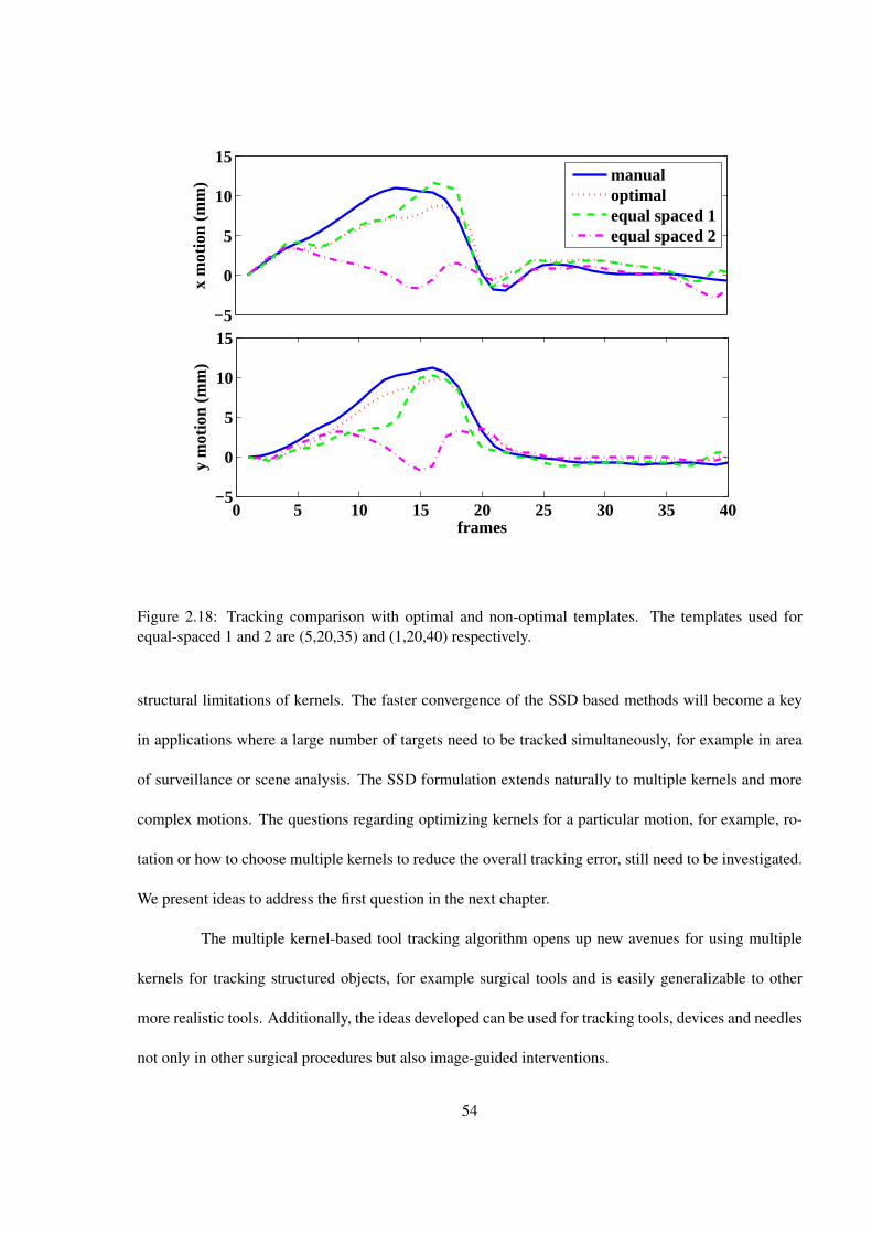
−5

0

5

10

15

x m

otio

n (m

m)

0 5 10 15 20 25 30 35 40−5

0

5

10

15

frames

y m

otio

n (m

m)

manualoptimalequal spaced 1equal spaced 2

Figure 2.18: Tracking comparison with optimal and non-optimal templates. The templates used forequal-spaced 1 and 2 are (5,20,35) and (1,20,40) respectively.

structural limitations of kernels. The faster convergence of the SSD based methods will become a key

in applications where a large number of targets need to be tracked simultaneously, for example in area

of surveillance or scene analysis. The SSD formulation extends naturally to multiple kernels and more

complex motions. The questions regarding optimizing kernels for a particular motion, for example, ro-

tation or how to choose multiple kernels to reduce the overall tracking error, still need to be investigated.

We present ideas to address the first question in the next chapter.

The multiple kernel-based tool tracking algorithm opens up new avenues for using multiple

kernels for tracking structured objects, for example surgical tools and is easily generalizable to other

more realistic tools. Additionally, the ideas developed can be used for tracking tools, devices and needles

not only in other surgical procedures but also image-guided interventions.

54

We have also presented a multiple template approach for tracking objects undergoing large

variations in appearance, especially targeted towards tracking cardiac structures in MR images. The

approach uses templates instead of an orthogonal basis thereby providing several advantages in terms of

their selection and online updating. It also allows for extension to bidirectional gradient methods that

allow much larger range of convergence for the local optimization. The algorithm validation for tracking

coronary arteries and cardiac valves in a range of MR images in different views is presented in Chapters 4

and 5.

55

Chapter 3

Optimal Kernels

As discussed in Chapter 1, tracking visual targets has emerged as a central problem in many

application areas such as surveillance, vision-based control, and human-computer interfaces. However,

despite the ubiquity of the tracking problem, the design and development of tracking algorithms is still

relatively ad-hoc. For a given application it is up to the designer to choose a set of methods that are likely

to perform well over the entire class of expected targets and target dynamics. Thus, the final design is a

compromise that works acceptably for all expected targets, but is likely to be sub-optimal on any given

target.

In this chapter, our goal is to develop a more principled design methodology around a notion

of optimal tracking. By stating and solving the problem based on objective optimization criteria, we

show that it is possible to create target-specific tracking algorithms that can significantly out-perform

commonly used “generic” algorithms. The basis for our methods lies in observing that recently developed

kernel-based tracking methods [25, 27, 57] can be viewed as a way of flexibly sampling multiple image

projections. As discussed in Section 2.1.1, many common image tracking methods can be modeled

through the choice of kernel structure, the number and spatial structure of sampling kernels, the choice

of image features space to operate on, and form of optimization used to compute location. Thus, spatial

56

sampling kernels form a basis for developing a large family of tracking algorithms. By making a good

choice of sampling kernel form, location and structure, it is possible to achieve robust, accurate tracking

for low computational cost.

The remainder of this chapter is structured as follows. In the next section, we briefly review

the limitations of the kernel-based tracking algorithms reviewed in the previous chapter. We then state

a version of the optimal tracking problem and develop several computationally efficient approximate

solutions. These solutions are evaluated on problems of interest and are generalized to more complex

problems.

3.1 Background

As discussed in the earlier section 2.1, the kernel-based tracking framework allows multiple

kernels and/or multiple image projections to be defined. Comaniciu et. al [25] defined multiple image

projections through a binning function into mutually orthogonal binary projections. In this case, the mo-

ments then become the fraction of the image region projecting into a particular bin, and the collection

forms a spatial image histogram. A single kernel placed at the center of the location space was used for

all the bands. Their work was extended by Hager et. al [27] to multiple kernels for tracking complex

motions. The idea of using motion specific kernels invariant to other motion parameters was introduced

but the kernels were still placed at the center and the same kernels were used for all the bands. The

idea of multiple kernels was further extended to articulated motions by [57]. Recent work on image

segmentation using kernel-based optimization shows the improvement in matching results by using mul-

tiple feature-space projections [58], thereby suggesting use of multiple projections can lead to improved

robust tracking results. It is interesting to note that if one places Gaussian kernels with small fixed band-

width at all the image locations in a target, the result is equivalent to conventional SSD tracking using a

Gaussian filter to pre-process the images [4]. Therefore, most kernel methods can be viewed as a special

57

case of template tracking arrived at by choosing several sampling kernels operating on several image

projections coupled through a set of photometric and geometric transformations.

One of the drawbacks of all the current approaches is that usually the same kernel is used for all

image projections and the kernel parameters (location and scale) are chosen in an ad-hoc manner. Figure

3.1 1 highlights the sub-optimality of the current kernel-based SSD method on a simple 1D step signal

as compared to that of an optimal kernel (see section 3.3). Using optimal kernels, the estimated shift

is very close to the true shift, whereas in the kernel-based SSD case the estimated shift is much lower

(aprroximately by a factor of 2).

It is easy to see if one could optimize the choice of sampling kernels over kernel parame-

ters (e.g. bandwidth), choice of image projection, and choice of kernel location, it may be possible to

greatly improve the tracking results and, at the same time, reduce computational cost. More recently, Fan

et. al. [59] proposed a gradient based algorithm for optimally placing kernels. The algorithm searches

locally for a kernel with a jacobian that has the lowest condition number in the neighborhood of the

initialization. They initialize the optimization at a grid or near the points of interest to select multiple

kernels with jacobians of good condition number. They show improved tracking results using multiple

optimal kernels. One of the limitation of the method is that the approach is local and initialization de-

pendent. In this section, we present our efforts towards developing a more principled framework for the

design of target-specific optimal kernels for tracking. We wish to note that this work is an extension and

generalization of the work in [60] that was limited primarily to roof or triangular kernels.

3.2 Problem Formulation

In this section, we define the notion of optimal tracking in the least mean square sense, and

show how the problem can be solved to design kernels for tracking a specific target in an image in an

1Return map is a plot showing the relationship between the estimated and true shift of a signal for a particular estimator

58

−10 −5 0 5 10−10

−5

0

5

10

shift in the rect signal

corr

ecti

on

aft

er f

irst

iter

atio

n

kernel SSD (epan kernel)kernel SSD (roof kernel)optimal kernel (gaussian)optimal kernel (square)

0 10 20 30 40 50 60 70 80−0.2

0

0.2

0.4

0.6

0.8

1

1.2

1.4

1.6

1.8

target sigopt ker (square)opt ker (gaussian)roof ker epan ker

Figure 3.1: Return map comparison between kernel-based SSD [27] and optimal kernels on a step signal(left). The right plot shows the step signal, the estimated optimal kernels (see section 3.3) and epan androof kernels used for kernel-based SSD. Note that in the kernel-based SSD method, the kernel is placedat the center with the scale equal to the size of the signal.

59

optimal or approximately optimal fashion. In the current formulation, we assume that the target region

in the image is generated by a simple additive model that is composed of a foreground (target) signal,

a background signal and noise signals. We use the notation developed in Chapter 2. Let f(x) and b(x)

be the foreground and background signals respectively. The foreground signal is generated primarily

from the object of interest being tracked whereas the background signal comes from the surrounding

objects/scene. So the generated target image at a given time t can be written as

G(x,τ(t), t) = f(T(x,τ(t)))+b(T(x,τ(t))+n(x, t) (3.1)

where n(x, t) is a random additive noise at the location x at time t and T(x,τ(t)) is a general transfor-

mation that acts on a location x and depends on a set of parameters τ(t) ∈ Rm at current time t. The

noise is a white noise with a Dirac delta autocorrelation function in both space and time. The image

at time t can be written using the same generative model as I(y,τ(t), t) = G(y,τ(t), t),∀ y ∈ Y. In the

current formulation, we put no restriction on the number of bands in the image signal i.e. the image can

be multi-dimensional.

In the tracking framework, the parameters τ(t) which define the motion of the region of in-

terest in image I(t) need to be estimated. Let τ(t) = h(I(y,τ( j), t),X); j = 1...(t−1) be a function that

estimates the value of the parameters at t. The function h depends on the current image, the pixel loca-

tions of the target region and the history of the parameter values. Since there are many possible ways of

estimating the parameters, a criterion is needed to evaluate different estimators.

Clearly, the choice of optimal h will depend on the characteristics of the target in question,

and also the expected range of variation of target motion. Thus, we consider the parameters τ to also be

modelled as a random variable. For a fixed h, this implies that τ(t) is now a random variable as it is a

function of τ and n. We can now state a mean square evaluation criterion as

e = En,τ

(m

∑i=1

(τ i− τ i)2

)(3.2)

60

where e is the mean square error that needs to be minimized and the expectation E is taken over both the

random variable τ and the noise n. It is worth noting that this is quite close to the basic form used to

derive the Kalman Filter [61]. Indeed, simply linearizing the above form and following the same form of

derivation leads to a Kalman filter-like form of a canonical SSD tracking [5] framework.

In this chapter, however, we take a slightly different approach. We consider a particular estima-

tor that uses kernels to weight samples in the target image. The idea behind the estimator can be derived

from the conventional tracking framework. Let us define Gr as the image of the target region when the

transformation parameters are zero; we will refer to this as the “reference template.” As the background

signal in this reference template is zero, it can be written as Gr(x) = f(T(x,0))+ n(x) = f(x)+ n(x).

Note that when τ = 0, the transformation has no effect on the location i.e. T(x,0) = x. The target re-

gion at a current time t is given by (3.1) with τ = τ(t) that needs to estimated. Let k : R2 → Rm be a

multi-dimensional kernel function composed of multiple single-dimensional kernel functions such that

k = [k1,k2, ...,km]T . Each kernel function ki, i = 1...m can be thought of as being associated with the ith

transformation parameter. The estimator can be derived by minimizing the following sum of squared

difference functional ∥∥∥∥∫x∈Xk(x)(G(x,τ(t))−Gr(T(x, τ(t)))) dx

∥∥∥∥2

(3.3)

where ‖‖ is the l2 norm. As with canonical SSD tracking [4, 5], the basic idea here is to estimate the

parameters that can transform the reference template to obtain the current target region. Now, using first

order Taylor series approximation about τ = 0, the following expression is obtained

∥∥∥∥∫x∈Xk(x)(G(x,τ(t))−Gr(x)) dx−D∗ τ(t)

∥∥∥∥2

(3.4)

where D = ddτ(t)

∫x∈X k(x)Gr(T(x,τ(t))) dx

∣∣∣τ(t)=0

. Minimizing the functional in (3.4) w.r.t. τ(t) ,the

estimate of the parameters is given by

τ = D†∫

x∈Xk(x)(G(x,τ(t))−Gr(x)) dx (3.5)

61

where D† is the pseudo inverse of D. Note that the rank of D has to be at least m for solution in (3.5)

to exist. Another assumption that has been made is that τ(t) is small. As usual, in practice the current

template (or reference template) is warped with the parameter value at the previous step τ(t−1) and the

change in parameter value ∆τ = τ(t)− τ(t−1) is then solved for in (3.5) [4, 5].

Using the derivatives of the image causes the convergence and hence estimation to be depen-

dent on the local fluctuation of the image gradient structure. If we can instead use the smooth and

analytical derivatives of a kernel, the parameters of the kernel can be chosen in such a way to yield better

convergence properties. In order to do this, a change of integration variables to y = T(x,τ(t)) is done to

move the geometric transformation onto the kernel. Doing so, the D matrix then becomes

D =d

dτ(t)

∫y∈Y

k(T−1(y,τ(t)))Gr(y))∣∣∣∣∂T−1

∂x

∣∣∣∣ dy

∣∣∣∣∣∣τ(t)=0

(3.6)

where Y = T(x,τ(t))∀x ∈ X. Substituting (3.5) in (3.2), we obtain the final expression that should be

minimized

e = En,τ

(∥∥∥∥D†∫

x∈Xk(x)(G(x,τ(t))−Gr(x)) dx− τ

∥∥∥∥2)

(3.7)

In this form, we can now view the choice of kernel k as a free parameter that can be optimized

to reduce this error.

3.3 Simple One Dimensional Case

Let us consider a simple one dimensional signal and a single unknown location parameter u.

The transformation T is:

T (x) = x−u (3.8)

Substituting into equation (3.1), we have

g(x,u) = f (x−u)+b(x−u)+n(x); (3.9)

62

Let the target region X = [c,d] (c < d). The estimator (3.5) becomes

u = D−1∫ d

cK(x)(g(x,u)−gr(x)) dx (3.10)

where gr(x) = f (x)+n(x) and D is now given by

D =ddu

∫ d−u

c−uk(x+u) f (x) dx

∣∣∣∣u=0

=∫ d

ck′(x) f (x) dx− k(d) f (d)+ k(c) f (c)

(3.11)

where k′(x) = ddx k(x).

Now, to obtain the optimal kernel, (3.7) is minimized to get

e = En,u

[(D−1

∫ d

ck(x)( f (x−u)− f (x)+b(x−u)

+n(x)) dx−u)2]

= En,u

[(e f + eb + en)

2]

(3.12)

where

e f = D−1∫ d

ck(x)( f (x−u)− f (x)) dx−u (3.13a)

eb = D−1∫ d

ck(x)b(x−u) dx (3.13b)

en = D−1∫ d

ck(x)n(x) dx (3.13c)

where n is the difference between the noise random variables in the current target image and the reference

template. In the current formulation we consider n to be a zero mean normal random variable N (0,σn).

The distribution for n is then given by N (0,√

2σn). We assume independence between u and n i.e.

p(n,u) = p(n)p(u) where p(n) and p(u) are p.d.f’s for n and u random variables and p(n,u) is their joint

density. This leads to the vanishing of the following cross term

En,u [(e f + eb)en] = 0 (3.14)

as E[n] = 0. Thus (3.12) becomes

63

e = En,u[(e f + eb)2 + e2

n]

(3.15)

Now, let us consider the error term e2n. The expectation is only taken over n as e2

n is independent of u.

En,u[e2n] = En,u

[D−2

∫ d

ck(x)n(x) dx

∫ d

ck(x′)n(x′) dx′

]= D−2

∫ d

c

∫ d

ck(x)k(x′)En

[n(x)n(x′)

]dx dx′

= 2D−2σ

2n

∫ d

ck2(x) dx

(3.16)

The last equality in (3.16) holds because En [n(x)n(x′)] = 2σ2n δ (x−x′) where δ is the dirac delta function.

The remaining term in (3.15) can be written as

En,u[(e f + eb)2]= Eu

[D−2

(∫ d

ck(x)( f (x−u)− f (x)

+ b(x−u)) dx−u)2] (3.17)

This expression can be easily numerically integrated by artificially shifting the signal to generate f (x−

u)+b(x−u) for different u’s. It is also possible to approximate the expression in (3.17) through a change

of coordinates as in (3.6), linearizing k(x) upto second order and neglecting the cross terms. Depending

on how the integration outside the range x ∈ [c,d] is treated, different approximations can be obtained.

For example, using the trapezoidal rule for integration, the following expression is obtained

En,u[(e f + eb)2]≈ 1

4D−2

{e2

f 1E[u2]+ (e f 4 + e f 2)2 E[u4]

+14

e2f 3E[u6]− k(c)k(d)E

[u2s(c−u)s(d−u)

]+ k2(c)E

[(us(c−u))2]+ k2(d)E

[(us(d−u))2]} (3.18)

The rectangular rule results in a much simpler expression:

En,u[(e f + eb)2]≈ D−2

{(12

e f 4 + e f 2

)2

E[u4]

+14

e2f 3E[u6]

} (3.19)

64

where

e f 1 = k(d) f (d)− k(c) f (c) (3.20a)

e f 2 = k′(c) f (c)− k′(d) f (d) (3.20b)

e f 3 = k′′(c) f (c)− k′′(d) f (d) (3.20c)

e f 4 =∫ d

ck”(x) f (x) dx (3.20d)

s(x−u) = ( f (x−u)+b(x−u)) (3.20e)

and k′′(x) = d2

d2x k(x). The expectation in the last two terms in (3.18) can be computed offline from the

background and foreground signals. Subsequently, we will refer to (3.18) as "approx 1" and (3.19) as

"approx 2".

To make the problem tractable, we restrict ourselves to two parametric families of normalized

kernels, namely square and gaussian kernels. We define

ks(x) =

0 if x−µs

σs> 1

34σs

(1−(

x−µsσs

)2)

otherwise

kg(x) =1√

2πσgexp

(−

(x−µg)2

2σ2g

)

where ks(x) is a normalized square kernel with parameters µs,σs and kg(x) is a normalized gaussian kernel

with parameters µg,σg. Now, the problem becomes one of finding these parameters such that (3.15) is

minimized. This can be done by numerical integration by subsituting (3.16) and (3.17) in (3.15). As

the numerical integration is more computationally expensive, (3.18) or (3.19) can be used to obtain an

approximate solution. For all optimizations in the paper, we use the matlab optimization toolbox function

fmincon and the parameters are limited between 1 and b−a, the length of the reference signal. With good

initialization, the time for this optimization is on the order of a minute.

In order to fully instantiate the model, we must choose a distributional form for the random

65

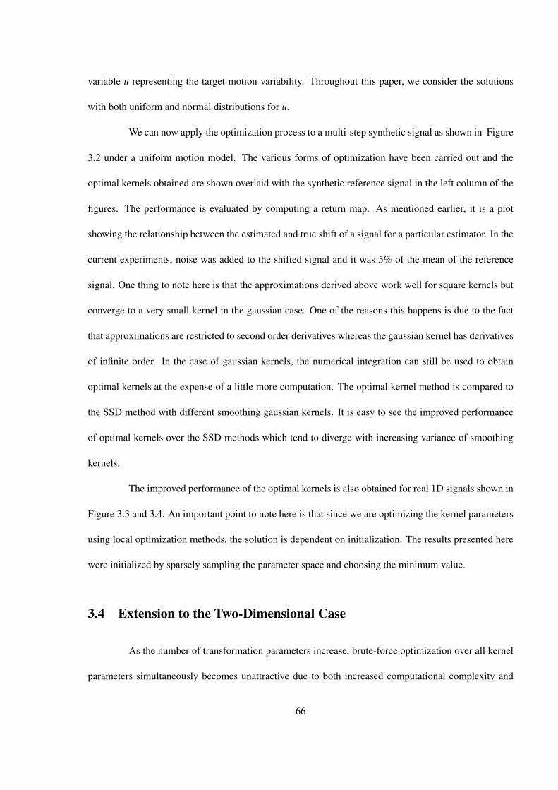
variable u representing the target motion variability. Throughout this paper, we consider the solutions

with both uniform and normal distributions for u.

We can now apply the optimization process to a multi-step synthetic signal as shown in Figure

3.2 under a uniform motion model. The various forms of optimization have been carried out and the

optimal kernels obtained are shown overlaid with the synthetic reference signal in the left column of the

figures. The performance is evaluated by computing a return map. As mentioned earlier, it is a plot

showing the relationship between the estimated and true shift of a signal for a particular estimator. In the

current experiments, noise was added to the shifted signal and it was 5% of the mean of the reference

signal. One thing to note here is that the approximations derived above work well for square kernels but

converge to a very small kernel in the gaussian case. One of the reasons this happens is due to the fact

that approximations are restricted to second order derivatives whereas the gaussian kernel has derivatives

of infinite order. In the case of gaussian kernels, the numerical integration can still be used to obtain

optimal kernels at the expense of a little more computation. The optimal kernel method is compared to

the SSD method with different smoothing gaussian kernels. It is easy to see the improved performance

of optimal kernels over the SSD methods which tend to diverge with increasing variance of smoothing

kernels.

The improved performance of the optimal kernels is also obtained for real 1D signals shown in

Figure 3.3 and 3.4. An important point to note here is that since we are optimizing the kernel parameters

using local optimization methods, the solution is dependent on initialization. The results presented here

were initialized by sparsely sampling the parameter space and choosing the minimum value.

3.4 Extension to the Two-Dimensional Case

As the number of transformation parameters increase, brute-force optimization over all kernel

parameters simultaneously becomes unattractive due to both increased computational complexity and

66

0 20 40 60 80 100 1200

0.5

1

1.5

2

2.5

3

target sigopt ker (approx 1)opt ker (approx 2)opt ker (numerical)

−20 −15 −10 −5 0 5 10 15 20−25

−20

−15

−10

−5

0

5

10

15

20

25

SSD(sigma=1)SSD(sigma=5)SSD(sigma=9)ground truthopt ker (approx 1)opt ker (approx 2) opt ker (numerical)

0 20 40 60 80 100 1200

1

2

3

4

5

6

target sigopt ker (approx 1)opt ker (approx 2)opt ker (numerical)

−20 −15 −10 −5 0 5 10 15 20−30

−20

−10

0

10

20

30

shift in the signal

Cor

rect

ion

afte

r 1s

t it

erat

ion

Comparison of SSD and optimal kernel methods

SSD(sigma=1)SSD(sigma=5)SSD(sigma=9)ground truthopt ker (approx 1)opt ker (approx 2) opt ker (numerical)

Figure 3.2: Comparison of SSD and optimal kernel methods on an artificial multiple step signal. The topand bottom rows show the results using square and gaussian kernels respectively. A uniform model for uis used for both kernels.

0 20 40 60 80 100 1200

10

20

30

40

50

60

70

target sigopt ker (numerical)

−20 −15 −10 −5 0 5 10 15 20−25

−20

−15

−10

−5

0

5

10

15

20

shift in the signal

corr

ecti

on a

fter

1st

iter

atio

n

Comparsion of SSD and optimal kernel methods

SSD (sigma = 1)SSD (sigma = 5)SSD (sigma = 9)ground truthoptimal kernel (numerical)

Figure 3.3: Comparison of SSD and optimal kernel methods on a real signal with gaussian kernels.Numerical integration with uniform model for u is used.

67

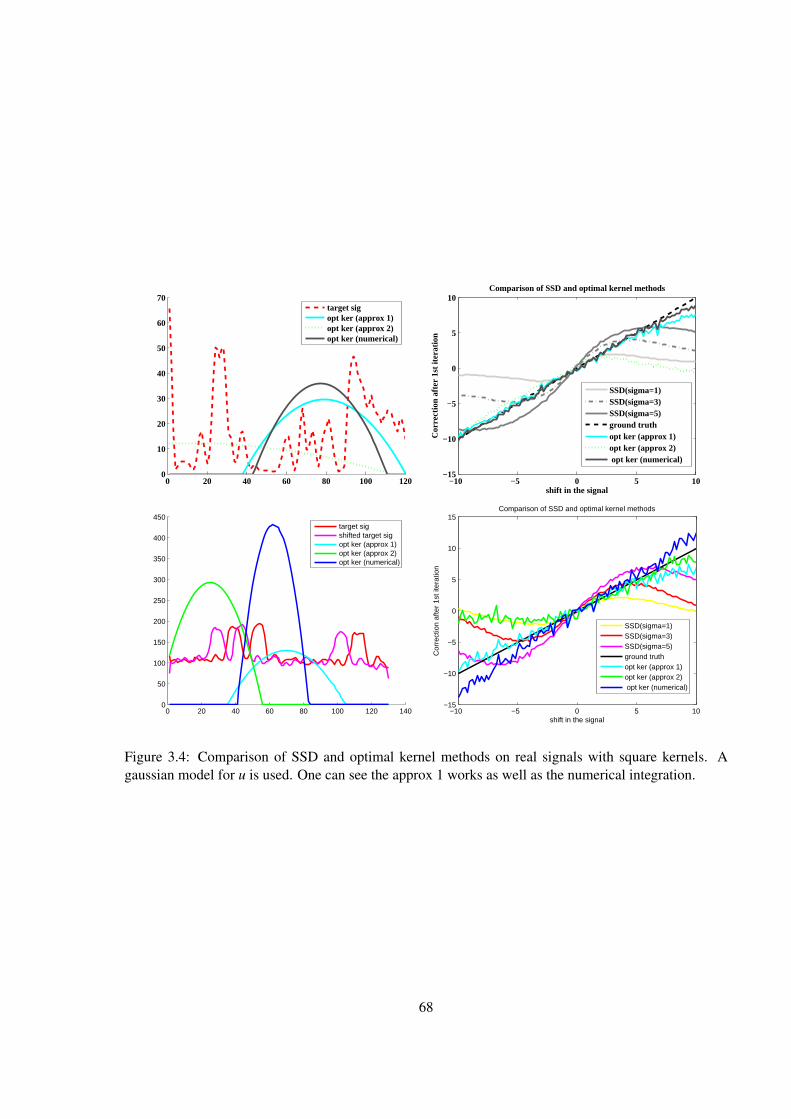
0 20 40 60 80 100 1200

10

20

30

40

50

60

70

target sigopt ker (approx 1)opt ker (approx 2)opt ker (numerical)

−10 −5 0 5 10−15

−10

−5

0

5

10

shift in the signal

Cor

rect

ion

afte

r 1s

t it

erat

ion

Comparison of SSD and optimal kernel methods

SSD(sigma=1)SSD(sigma=3)SSD(sigma=5)ground truthopt ker (approx 1)opt ker (approx 2) opt ker (numerical)

0 20 40 60 80 100 120 1400

50

100

150

200

250

300

350

400

450

target sigshifted target sigopt ker (approx 1)opt ker (approx 2)opt ker (numerical)

−10 −5 0 5 10−15

−10

−5

0

5

10

15

shift in the signal

Cor

rect

ion

afte

r 1s

t ite

ratio

n

Comparison of SSD and optimal kernel methods

SSD(sigma=1)SSD(sigma=3)SSD(sigma=5)ground truthopt ker (approx 1)opt ker (approx 2) opt ker (numerical)

Figure 3.4: Comparison of SSD and optimal kernel methods on real signals with square kernels. Agaussian model for u is used. One can see the approx 1 works as well as the numerical integration.

68

the presence of many local minimums. Also, it is difficult to obtain any reasonable approximations

using the methods applied to the one-dimensional case. The question we would like to ask is : Can we

decouple the optimization in (3.7) for the two-dimensional case into two one-dimensional optimizations

and then use the results derived in the one-dimensional case for optimizing kernels in two-dimensions?

Reducing the problem into one-dimension avoids a large number of local minimums apart from making

the optimization faster. Also, simple 1D approximations can be applied to reduce the computation time.

Another advantage is that the two-dimensional optimization can be initialized with the solutions obtained

from one-dimensional optimization to further fine tune the solution. In this section, we discuss the

optimization in the two-dimensional case based on the ideas developed in [60].

To be more specific, let us consider the two-dimensional case where the transformation T is

given by

T(x,(u,v)) = [x−u,y− v]T

where x = (x,y) and (u,v) are the transformation parameters. Let X = {(cx ≤ x ≤ dx),(cy ≤ y≤ dy)} be

the target region. The image generation equation (3.1) becomes

g((x,y),(u,v)) = f (x−u,y− v)+b(x−u,y− v)+n(x,y)

As presented in [60], the basic idea involves decoupling (3.5) to optimize kernels for the transformation

parameters u and v independently. Let us define Kx(x,y) and Ky(x,y) to be kernels optimizing u and v

respectively. If we consider these kernels to be composed of separable kernels s.t. Kx(x,y) = kxx(x)kxy(y)

and Ky(x,y) = kyx(x)kyy(y), then the individual de-coupled transformation estimation equations can be

defined as

u = D−1x

∫ dx

cx

kxx(x)[gx(x)− fx(x)] dx (3.21a)

v = D−1y

∫ dy

cy

kyy(y)[gy((y))− fy(y)] dy (3.21b)

69

where

gx =∫ dy

cy

kxy(y)g((x,y),(u,v)) dy (3.22a)

fx =∫ dy

cy

kxy(y) f (x,y) dy (3.22b)

Dx =ddu

∫ dx

cx

kxx(x+u) fx(x) dx∣∣∣∣u=0

(3.22c)

and

gy =∫ dx

cx

kyx(x)g((x,y),(u,v)) dx (3.23a)

fy =∫ dx

cx

kyx(x) f (x,y) dx (3.23b)

Dy =ddv

∫ dy

cy

kyy(y+ v) fy(y) dy∣∣∣∣v=0

(3.23c)

The simple trick used here is that kernels kxy(y) and kyx(x) project both the current target g((x,y),(u,v)

and reference target f (x,y) into one dimensional signals that depends on either x or y, depending on

the kernel being used. Now, given kxy(y) and kyx(x), optimal kxx(x) and kyy(y) can be easily computed

using the methods developed in the section 3.3. One of the drawbacks in the current form is that the

performance of the estimators (3.21a) and (3.21b) will be affected by the other transformation parameter

v and u respectively. To reduce this effect, we take the following approach. For simplicity, the approach

is explained through the estimation of Kx(x,y) and a similar procedure can be followed for estimating

Ky(x,y). One way to reduce the effect of v on the estimation of kxx(x) is to optimize the parameters for

kxy(y) such that (3.21a) becomes invariant to v. By invariance here we mean that the transformation v

should not affect the estimation in parameter u. This can be done by numerical integration as discussed

in section 3.3. Thus, as shown in Figure 3.5 the estimation of Kx(x,y) becomes a two-step iterative

optimization.

1. Depending on the kernel choice, initialize the parameters of kxx(x) and kxy(y) to reasonable values.

The initialization of the center of the kernels will be discussed later.

70

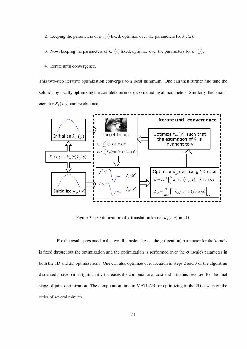
2. Keeping the parameters of kxy(y) fixed, optimize over the parameters for kxx(x).

3. Now, keeping the parameters of kxx(x) fixed, optimize over the parameters for kxy(y).

4. Iterate until convergence.

This two-step iterative optimization converges to a local minimum. One can then further fine tune the

solution by locally optimizing the complete form of (3.7) including all parameters. Similarly, the param-

eters for Ky(x,y) can be obtained.

Figure 3.5: Optimization of x-translation kernel Kx(x,y) in 2D.

For the results presented in the two-dimensional case, the µ (location) parameter for the kernels

is fixed throughout the optimization and the optimization is performed over the σ (scale) parameter in

both the 1D and 2D optimizations. One can also optimize over location in steps 2 and 3 of the algorithm

discussed above but it significantly increases the computational cost and it is thus reserved for the final

stage of joint optimization. The computation time in MATLAB for optimizing in the 2D case is on the

order of several minutes.

71

Since the center of the kernels are fixed, it is important to initialize them near good locations

to obtain better convergence. We have developed a simple automatic heuristic that operates as follows:

1. Compute Canny edges in the image.

2. Choose pairs of edge points and compute the magnitude of the cross product of the image gradient

at that point.

3. Apply kernel optimization to the top few (e.g. 5 to 10) pairs and choose the final result with lowest

expected error.

In particular, note the ranking in step 2 above favors edge pairs that are roughly orthogonal and have

large gradient magnitude.

We now put all of this together to demonstrate the results of choosing kernels for two-dimensional

translation. The results shown here are using gaussian kernels although similar results can be obtained

using square kernels. First, a simple synthetic image shown at the left in Figure 3.6 was used to compute

the two-dimensional return map. One can see that the optimal kernel outperforms SSD with different

smoothing gaussian kernels even for twice the optimized range. In this case, the initial point were man-

ually selected at the horizontal and vertical edge.

Figure 3.7 shows the results when the location is selected with the heuristic algorithm dis-

cussed above. The first and second row shows the results of templates chosen from a clown image in

matlab and coronal view MRI image respectively. The top 10 selected image pairs are shown in the first

column overlaid over the template. The green and red color corresponds to initialization points for x

and y translation kernels respectively. The return map comparisons shown in the right column shows the

improved performance of optimal kernels. Although one of the SSD results is comparable to the optimal

kernel performance but usually the optimal sigma value for SSD is not known before hand. Also as

mentioned in section 3.1, kernel-based methods can be thought of as a special case of SSD.

72

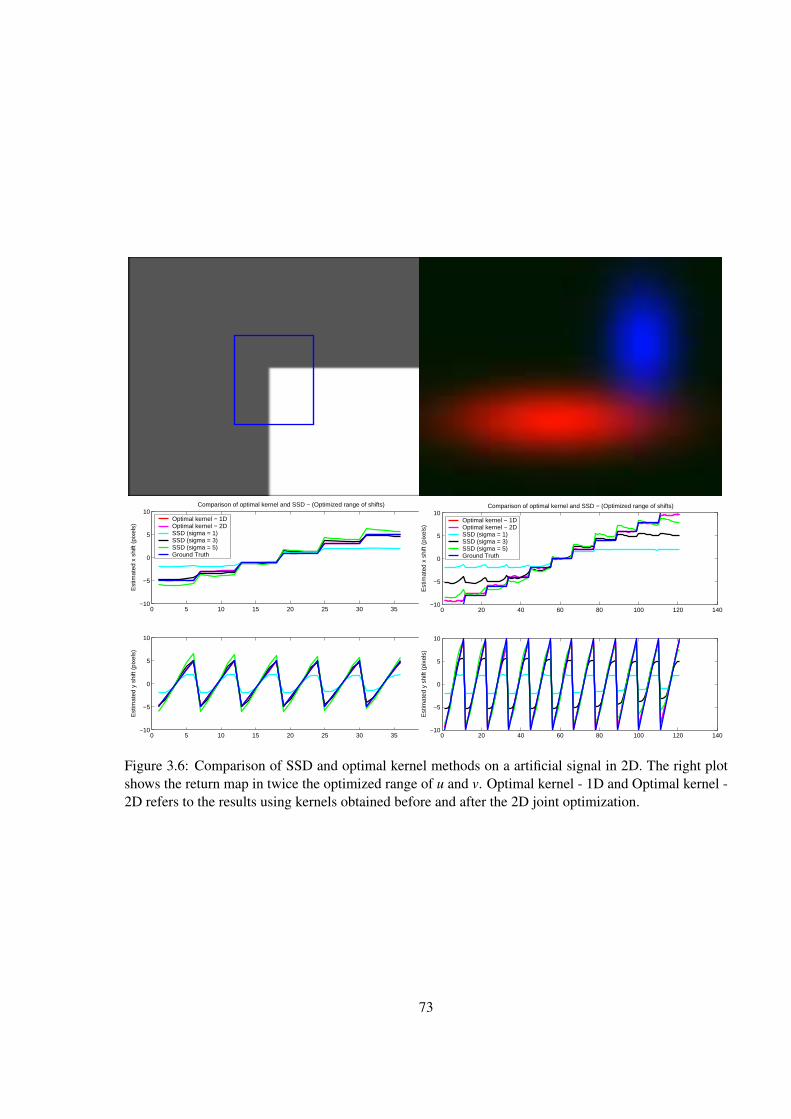
0 5 10 15 20 25 30 35 40−10

−5

0

5

10

Est

imat

ed x

shi

ft (p

ixel

s)

Comparison of optimal kernel and SSD − (Optimized range of shifts)

Optimal kernel − 1DOptimal kernel − 2DSSD (sigma = 1)SSD (sigma = 3)SSD (sigma = 5)Ground Truth

0 5 10 15 20 25 30 35 40−10

−5

0

5

10

Est

imat

ed y

shi

ft (p

ixel

s)

0 20 40 60 80 100 120 140−10

−5

0

5

10

Est

imat

ed x

shi

ft (p

ixel

s)

Comparison of optimal kernel and SSD − (Optimized range of shifts)

Optimal kernel − 1DOptimal kernel − 2DSSD (sigma = 1)SSD (sigma = 3)SSD (sigma = 5)Ground Truth

0 20 40 60 80 100 120 140−10

−5

0

5

10

Est

imat

ed y

shi

ft (p

ixel

s)

Figure 3.6: Comparison of SSD and optimal kernel methods on a artificial signal in 2D. The right plotshows the return map in twice the optimized range of u and v. Optimal kernel - 1D and Optimal kernel -2D refers to the results using kernels obtained before and after the 2D joint optimization.

73

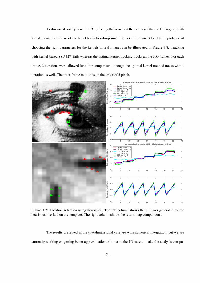
As discussed briefly in section 3.1, placing the kernels at the center (of the tracked region) with

a scale equal to the size of the target leads to sub-optimal results (see Figure 3.1). The importance of

choosing the right parameters for the kernels in real images can be illustrated in Figure 3.8. Tracking

with kernel-based SSD [27] fails whereas the optimal kernel tracking tracks all the 300 frames. For each

frame, 2 iterations were allowed for a fair comparison although the optimal kernel method tracks with 1

iteration as well. The inter-frame motion is on the order of 5 pixels.

1a

1b2a2b

3a

3b

4a

4b

5a

5b

6a

6b

7a

7b

8a

8b

9a

9b

10a

10b0 5 10 15 20 25 30 35 40

−10

−5

0

5

10

Est

imat

ed x

shi

ft (p

ixel

s)

Comparison of optimal kernel and SSD − (Optimized range of shifts)

Optimal kernel − 1DOptimal kernel − 2DSSD (sigma = 1)SSD (sigma = 3)SSD (sigma = 5)Ground Truth

0 5 10 15 20 25 30 35 40−10

−5

0

5

10

Est

imat

ed y

shi

ft (p

ixel

s)

1a

1b

2a

2b

3a

3b

4a

4b

5a

5b

6a

6b

7a

7b

8a

8b

9a

9b

10a

10b

0 5 10 15 20 25 30 35 40−10

−5

0

5

10

Est

imat

ed x

shi

ft (p

ixel

s)

Comparison of optimal kernel and SSD − (Optimized range of shifts)

Optimal kernel − 1DOptimal kernel − 2DSSD (sigma = 1)SSD (sigma = 3)SSD (sigma = 5)Ground Truth

0 5 10 15 20 25 30 35 40−10

−5

0

5

10

Est

imat

ed y

shi

ft (p

ixel

s)

Figure 3.7: Location selection using heuristics. The left column shows the 10 pairs generated by theheuristics overlaid on the template. The right column shows the return map comparisons.

The results presented in the two-dimensional case are with numerical integration, but we are

currently working on getting better approximations similar to the 1D case to make the analysis compu-

74

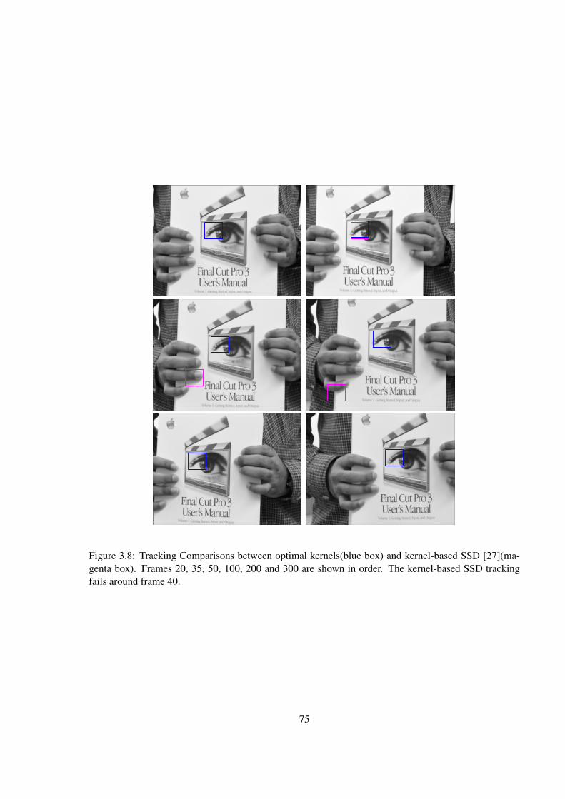
Figure 3.8: Tracking Comparisons between optimal kernels(blue box) and kernel-based SSD [27](ma-genta box). Frames 20, 35, 50, 100, 200 and 300 are shown in order. The kernel-based SSD trackingfails around frame 40.

75

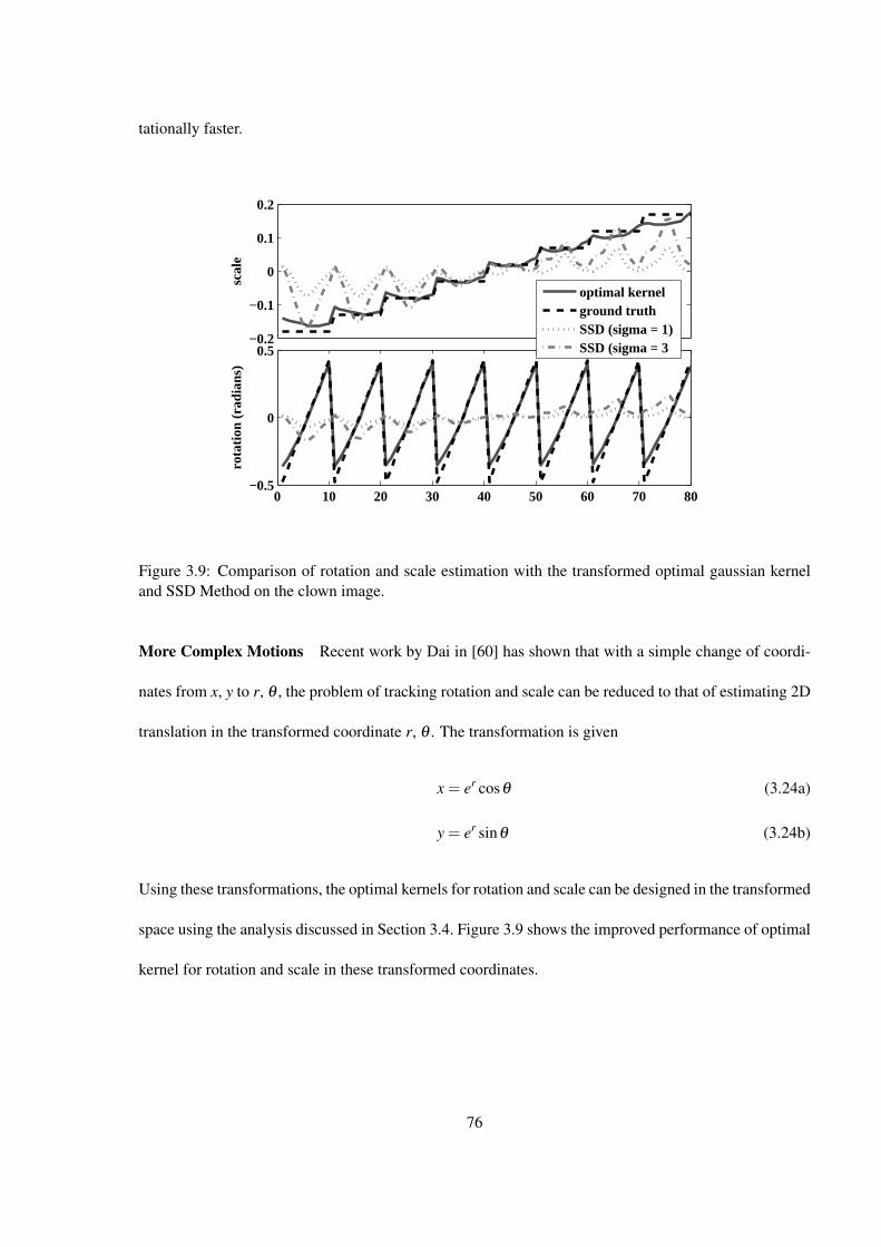
tationally faster.

−0.2

−0.1

0

0.1

0.2

scal

e

0 10 20 30 40 50 60 70 80−0.5

0

0.5

rota

tion

(ra

dian

s)

optimal kernelground truthSSD (sigma = 1)SSD (sigma = 3

Figure 3.9: Comparison of rotation and scale estimation with the transformed optimal gaussian kerneland SSD Method on the clown image.

More Complex Motions Recent work by Dai in [60] has shown that with a simple change of coordi-

nates from x, y to r, θ , the problem of tracking rotation and scale can be reduced to that of estimating 2D

translation in the transformed coordinate r, θ . The transformation is given

x = er cosθ (3.24a)

y = er sinθ (3.24b)

Using these transformations, the optimal kernels for rotation and scale can be designed in the transformed

space using the analysis discussed in Section 3.4. Figure 3.9 shows the improved performance of optimal

kernel for rotation and scale in these transformed coordinates.

76

3.5 Conclusions

In this chapter, we have presented an objective approach for developing optimal tracking meth-

ods, and have demonstrated this approach for the specific case of kernel-based tracking. In particular,

we have shown that these methods can be performed using effective approximations for one-dimensional

and two-dimensional cases, and we have suggested how this can be generalized to higher-dimensional

problems. The results on several examples illustrate the potential advantages of such optimizations.

These results point the way toward a more principled and consistent methodology for the design of

visual tracking algorithms.

In future, we plan to extend the approach to choose multiple kernels and multiple features

spaces. Additionally, the coupling of optimal tracking with a surrounding predictor-estimator is of in-

terest. As noted previously, the optimization criterion we use is closely related to that used in classical

optimal estimator design. Thus, it seems likely that it will be possible to derive optimal time-series

estimators using models of target dynamics to further improve the performance of these algorithms.

77

Chapter 4

Beat-to-Beat Motion Compensation for

Robust Coronary MR Angiography

4.1 Introduction

Coronary Angiography refers to the imaging of the coronary arteries, the lifeline of the heart.

These arteries supply blood to the heart muscles that contract and relax to pump blood to the rest of the

body. There are two major coronary arteries that branch off from the aorta - the right coronary artery

(RCA) and the left main (LM) coronary artery. The left main coronary artery further branches into

the left circumflex (LCX) artery and the left anterior descending (LAD) artery as shown in Figure 4.1.

The coronary arteries can become narrowed or blocked through plaque deposits on the inner walls of

these arteries also known as atherosclerosis. This restricts the blood flow to the heart preventing it from

functioning normally leading to chest pain (or angina) and in severe cases can lead to a heart attack. This

condition is commonly known as the coronary artery disease (CAD).

CAD remains one of the major causes of morbidity and mortality in the United States, and is

increasing in prevalence in non-Western cultures as well [11]. The current gold standard for diagnosis is

78

Figure 4.1: The primary coronary arteries in the heart.

catheter-driven x-ray coronary angiography [62, 63, 64, 65]. During this procedure, a catheter is driven

into a blood vessel in the arm or leg, and guided into the coronary arteries in the heart under X-ray.

A contrast-dye is then injected through the catheter to obtain coronary angiograms. Unfortunately, this

procedure involves risks owing to its invasiveness, radiation exposure and use of potentially nephrotoxic

contrast agent. Therefore, a method for robust and noninvasive coronary artery screening is highly

desirable for the early detection of disease. Computed tomography (CT) and magnetic resonance imaging

(MRI) are good candidates and recently, have shown significant work in this direction. CT has the

advantage that images are acquired quickly and with relatively good spatial resolution, but uses ionizing

radiation and nephrotoxic contrast agents [66, 67, 68, 69]. MRI does not require the use of radiation,

but the speed of image acquisition is slow. It thus relies on data acquired over multiple heartbeats

either in a breath-hold with lower spatial resolution, or during free breathing with motion correction,

over a period of 5-10 minutes, for higher spatial resolution [70, 71, 72, 73, 74]. Both MRI and CT are

being used clinically for ventricular function, perfusion imaging, and infarct imaging. MRI has some

inherent advantages for soft tissue discrimination, and thus may be more suitable for vessel wall imaging

79

and early detection of atherosclerosis [75, 76, 77, 78]. Coronary MR has been shown to have good

accuracy for triple vessel and left main disease [79], but image quality varies widely across patients

and therefore is not robust for clinical use (currently 70-80% successful in practice). In addition current

spatial resolution for coronary MR is on the order of 0.7 - 1 mm in plane. The tortuous geometry of

the coronary arteries (see Figure 4.1) also puts forth a requirement in terms of volumetric coverage.

As the coronary arteries usually do not lie on a single two-dimensional plane, they require a volume

to be imaged, which translates into a longer data acquisition. Higher spatial resolution and volumetric

coverage in turn places higher demands on motion compensation during image acquisition. Therefore

in the area of noninvasive cardiovascular imaging, there is need to improve motion compensation for

coronary MR imaging, including both angiography and vessel wall imaging.

4.2 Previous Work

The coronary arteries undergo a complex motion induced by both respiratory and cardiac mo-

tion [13, 80]. Although the general motion pattern of the heart due to respiration and its own contrac-

tion/expansion is well known, there is no well-defined parameterized model that can be used to char-

acterize how the intricate combination of respiratory and cardiac motion results in the motion of the

coronary arteries. Furthermore, even on a single subject, there is variation between respiratory and car-

diac motion cycles as well as variation across patients. This makes it difficult to gauge and predict the

motion of the coronary arteries and compensate for that motion during MR imaging. Therefore, a simple

yet effective way to image the coronary arteries is to acquire imaging data when the effect of cardiac

and respiratory motion is minimal. Current methods achieve this by gating the data acquisition for both

respiratory and cardiac motion. For respiratory motion, one tracks the position of the diaphragm-lung

interface as a function of time using a 1D “navigator” which is then used to gate the data acquisition to

the end-expiratory part of the breathing cycle [72, 73]. To further improve the respiratory motion com-

80

pensation, some approaches use correlation between the acquired and the reference navigator echo to

compute motion within the acceptance window usually chosen around end-expiration. One then uses a

correction factor to transform the motion and use it for slice correction [72, 79, 81]. Hofman et al [82]

measured coronary motion using cine-MRI and estimated the amount of coronary motion during various

acquisition windows to determine the effect on blur in coronary MR images. Shechter et al also measured

coronary motion but from x-ray angiography and estimated required acquisition windows for coronary

MR [13]. It is thus generally well accepted that the effect of cardiac motion can be ameliorated by re-

stricting the data acquisition to a very small time window in the mid-diastole part of the cardiac cycle

where the heart motion is known to be minimal.Figure 4.2 shows the sequence diagram of a conventional

coronary Magnetic Resonance Acquisition (MRA) approach.

Figure 4.2: Current Approach for coronary MRA.

Current MRA methods suffer from robustness and repeatability in healthy volunteers as well as

in patients. The limitations of the current methods may be attributed to a combination of the following:

1. The assumption that the diaphragm motion and the coronary motion are correlated is not per-

81

fect [83, 84].

2. The relationship between diaphragm motion and coronary motion does not remain constant over a

10-15 minute image acquisition period [85, 86, 87, 88].

3. The motion of the various coronary arteries is dissimilar, with different timing of peak motion in

the cardiac cycle along with different absolute values of total displacement, velocity and accelera-

tion [82, 89].

4. During multiple heartbeats, the motion of the coronary arteries can vary from beat to beat in a

manner that cannot be predicted a priori [84, 15].

5. The ECG signal used to gate the cardiac motion compensated data acquisition, although known to

be correlated with global cardiac motion, does not necessarily correlate with the coronary motion

which further deteriorates in patients especially those with cardiac arrhythmias [82, 90].

6. Finally, there is variability of motion across subjects and patients [82, 84, 89].

4.2.1 Respiratory Motion Variability

Various methods have been tried over the last few years to address the first limitation (men-

tioned above) with modest success. It has been shown that the use of navigator on the heart itself yields

slightly inferior results compared to the diaphragmatic navigator [15]. However, using additional nav-

igators on the heart in the anterior/posterior and the right/left direction along with the diaphragmatic

navigator (superior/inferior direction) does lead to an improvement in image quality [91]. The draw-

backs of these approaches are that they still assume correlation between heart motion and coronary

motion and there can be hysteretic effects during the respiratory cycle, thereby incorporating more er-

rors [92]. Nguyen et al. [93] proposed the use of cardiac fat NAV for respiratory motion compensation.

The cardiac fat NAV monitors the epicardial fat that surrounds the coronary arteries, moves together

82

with it, and thereby provides a direct measurement of bulk coronary artery motion. The cardiac fat NAV

approach showed improvement over the conventional diaphragmatic navigator approach and eliminated

the need for a subject-specific correction factor. The success of the approach was limited by the contam-

ination of the fat NAV by the chest wall signal and use of only the S/I displacement component of the

fat NAV. The problem of drift in the relationship between the diaphragm and coronary motion has been

addressed reasonably well by DVA [87] and PAWS [88] approaches along with reduction in the scanning

time especially in patients. Recently, a subject-specific method [94] has been proposed that builds a low

resolution motion model correlated with multiple navigators and uses the inverse model online during

scanning to correct for respiratory motion effects. Although this approach is subject-specific, it does not

address variability in cardiac motion and in long-term respiratory motion during an acquisition. The lim-

ited success of respiratory motion compensation methods proposed so far can be attributed to the recent

studies [95, 96] that demonstrate the need for an online subject-specific complex model to completely

characterize the motion of the coronary arteries due to respiration. A non-navigator based approach for

motion compensation using adaptive averaging was proposed by Hardy et al. [35]. In this approach,

cross correlation of real-time images of a slice containing the coronary artery was used to reduce motion

artifact by averaging. The major drawback of the approach was the restriction to 2D imaging and the

inability to account for through plane motions limiting the overall resolution.

4.2.2 Heart Rate and Cardiac Motion Variability

It is well known that the heart rate or the electrocardiographic RR interval fluctuates cyclically,

mediated predominantly through the autonomic nervous system via changes in sympathetic and parasym-

pathetic activity [97,98]. The significance of the heart rate variability (HRV) and its prognostic potential

during short-term electrocardiographic recordings (duration of 5-15 minutes) in both normal healthy and

patient populations has been quite well established now [99, 100, 101]. Standard measures of short-term

83

HRV for normal and patient populations have been reported in various studies [99,100,101]. Also, phys-

iological interactions between respiration and circulation affect the HRV and introduce a high-frequency

component of fluctuation in the RR interval variability [102]. This becomes an important factor during

free-breathing cardiovascular magnetic resonance imaging methods. It has also been shown that sys-

tolic time interval remains relatively constant [103] compared to the diastolic time period that varies to a

greater extent [104]. Also, while the systolic time interval decreases linearly with increasing heart rate,

the diastolic time interval on the other hand has a much larger curvilinear decrease [103, 104, 105].

Unlike respiration variability, the issue of heart rate variability for coronary MRA has not been

widely explored, with only a few methods proposed in recent years. Ustun et al. [106] proposed the

selection of a subject-specific minimal motion window during pre-scan. The approach improved image

quality but has the disadvantage that it does not account for heart rate variability during the acquisition.

Recent work on trigger delay adaptation through neural networks and adaptive averaging [107] has been

proposed to account for HR changes during the coronary MRA scan. However, this method included use

of the ECG signal instead of actual coronary motion data, use of the lung-diaphragm interface navigator

for respiratory compensation and did not account for beat-to-beat variability in cardiac motion.

Recent advances in accelerated parallel imaging has revived breath-hold coronary MRA [108,

109] eliminating the need for complicated methods for compensating for respiratory motion. Since these

approaches span multiple cardiac beats (usually around 30), they are still limited by the effects of beat-

to-beat cardiac variability. Breath-hold techniques though, have limited application in coronary MRA

as it has been observed that patients with coronary artery disease (CAD) have difficulty to both suspend

respiration and repeatedly hold breath at the same position as compared to normal subjects [110]. The

limited duration of breath-holds and continued diaphragmatic drifts during breath-hold [111] warrant

free-breathing approaches.

84

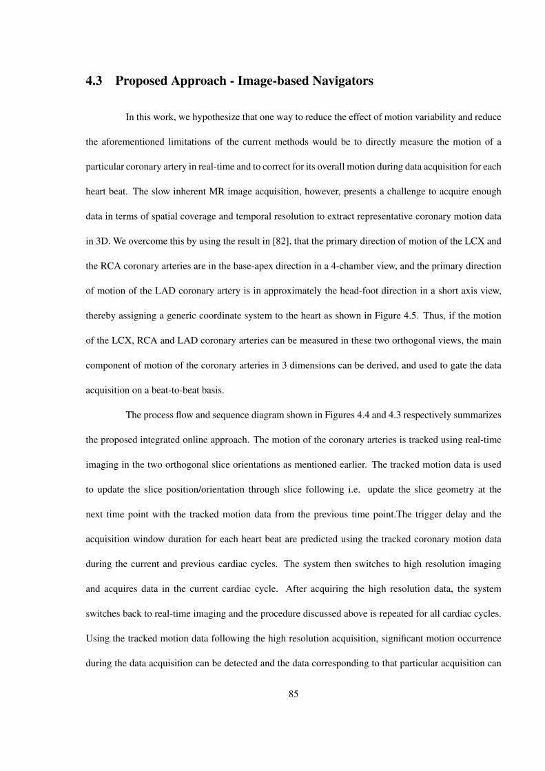
4.3 Proposed Approach - Image-based Navigators

In this work, we hypothesize that one way to reduce the effect of motion variability and reduce

the aforementioned limitations of the current methods would be to directly measure the motion of a

particular coronary artery in real-time and to correct for its overall motion during data acquisition for each

heart beat. The slow inherent MR image acquisition, however, presents a challenge to acquire enough

data in terms of spatial coverage and temporal resolution to extract representative coronary motion data

in 3D. We overcome this by using the result in [82], that the primary direction of motion of the LCX and

the RCA coronary arteries are in the base-apex direction in a 4-chamber view, and the primary direction

of motion of the LAD coronary artery is in approximately the head-foot direction in a short axis view,

thereby assigning a generic coordinate system to the heart as shown in Figure 4.5. Thus, if the motion

of the LCX, RCA and LAD coronary arteries can be measured in these two orthogonal views, the main

component of motion of the coronary arteries in 3 dimensions can be derived, and used to gate the data

acquisition on a beat-to-beat basis.

The process flow and sequence diagram shown in Figures 4.4 and 4.3 respectively summarizes

the proposed integrated online approach. The motion of the coronary arteries is tracked using real-time

imaging in the two orthogonal slice orientations as mentioned earlier. The tracked motion data is used

to update the slice position/orientation through slice following i.e. update the slice geometry at the

next time point with the tracked motion data from the previous time point.The trigger delay and the

acquisition window duration for each heart beat are predicted using the tracked coronary motion data

during the current and previous cardiac cycles. The system then switches to high resolution imaging

and acquires data in the current cardiac cycle. After acquiring the high resolution data, the system

switches back to real-time imaging and the procedure discussed above is repeated for all cardiac cycles.

Using the tracked motion data following the high resolution acquisition, significant motion occurrence

during the data acquisition can be detected and the data corresponding to that particular acquisition can

85

be reacquired. We refer to this approach as “image based navigators”. In order to make the approach

feasible in real-time we assume that the out of plane motion between frames would be relatively small

with slice following and that the duration of minimal motion of different segments of the coronary artery

are similar. Although, presently we are proposing a translation motion model for tracking and slice

updating, it is important to point out that the approach is general and more complex motion models

including rotations can be easily incorporated in the framework.

Figure 4.3: Basic sequence-timing diagram of the proposed approach using image-based navigators.

The primary goal of our work is to investigate the extent of the coronary artery motion vari-

ability, with focus on the proximal RCA, LCX and LAD coronary arteries and how a subject-specific

online proposed approach can be used to compensate for it. In particular:

86

Figure 4.4: Process flow in the proposed approach for coronary MRA.

1. We hypothesize that real-time imaging can be used to track these coronary arteries with sufficient

accuracy to compensate for beat to beat variability in coronary motion for reducing motion artifact

in high resolution coronary MR angiography. In order to accomplish this goal, we present the

development and validation of a motion tracking algorithm .

2. We hypothesize that the extent of cardiac motion variability during high resolution coronary imag-

ing is significant enough to affect image quality when fixed acquisition periods are used.

3. We also hypothesize that beat-to-beat compensation using the proposed approach can improve the

image quality and robustness of high resolution coronary MRA.

4. Finally, we validate previous work that the diaphragm motion and respiratory component of the

coronary motion are well correlated; and show that tracking the diaphragm motion is still insuffi-

cient for respiratory motion compensation.

In the current study, we explore the impact of this approach on image quality in an offline

implementation using human motion data, but without the online feedback loop shown in Figure 4.4. We

87

Figure 4.5: Subject-specific heart coordinate system. The X ′, Y ′ and Z′ axes of the heart coordinatesystem are shown in 4-chamber and short axis views separately in 2D (a) and in 3D (b).

88

would like to note that it is beyond the scope of this work to present a complete online implementation

of the proposed approach with combined real-time and high resolution imaging. Instead, our goal is to

present initial evidence that this approach would make an impact on image quality as a basis for further

development of an online integrated solution.

The remainder of the chapter is organized as follows. The parameters of the data acquired to

test the hypotheses are presented next. Then, the details of the tracking algorithm and its validation are

discussed. This is followed by a study to show the extent of heart rate variability during cardiac scans.

We then present a simulation using extracted human coronary motion that shows the improvement in

MR image quality when the cardiac variability is compensated for. Finally, we investigate how well the

lung-diaphragm interface motion can be used to compensate for the respiratory component of coronary

motion for coronary MRA.

4.4 Data Acquisition

In order to investigate the feasibility of the proposed image-based navigators, we acquired low

spatial resolution real-time (LSRRT) images in 5 healthy volunteers with the subjects breathing freely.

All subjects gave informed consent to a protocol approved by the local Institutional Review Board. The

data consists of real-time SSFP images in the short axis, 4-chamber and coronal views taken from the

5 volunteers (4 males, 1 female, age range 22 to 41) with the following parameters: TR/TE/FL = 2.18-

2.28/1.09-1.14/49-56, GRAPPA acceleration = 2, in plane reconstructed resolution = 2.76 - 2.89 mm,

slice thickness = 6 - 8mm, acquisition matrix size = 50 x 128 - 68 x 128 pixels, Interpolated matrix

size = 88 x 128 - 112 x 128 pixels, FOV = 243 x 354 - 324 x 370 mm, at 15-20 frames/sec for a total

of approximately 750 frames during free breathing on a 1.5T scanner (Espree, Siemens). In order to

validate the tracking, we also acquired both low resolution real-time (parameters same as mentioned

above for free-breathing data) and high resolution cine (HRC) images in all three views with the subjects

89

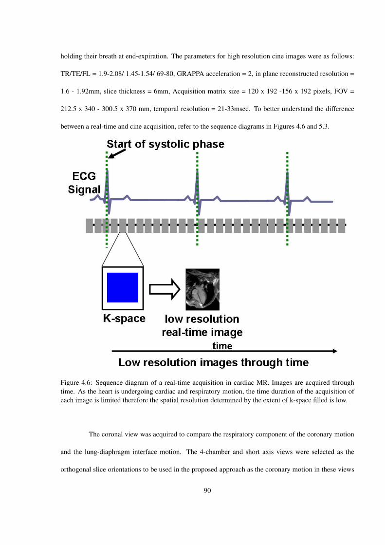
holding their breath at end-expiration. The parameters for high resolution cine images were as follows:

TR/TE/FL = 1.9-2.08/ 1.45-1.54/ 69-80, GRAPPA acceleration = 2, in plane reconstructed resolution =

1.6 - 1.92mm, slice thickness = 6mm, Acquisition matrix size = 120 x 192 -156 x 192 pixels, FOV =

212.5 x 340 - 300.5 x 370 mm, temporal resolution = 21-33msec. To better understand the difference

between a real-time and cine acquisition, refer to the sequence diagrams in Figures 4.6 and 5.3.

Figure 4.6: Sequence diagram of a real-time acquisition in cardiac MR. Images are acquired throughtime. As the heart is undergoing cardiac and respiratory motion, the time duration of the acquisition ofeach image is limited therefore the spatial resolution determined by the extent of k-space filled is low.

The coronal view was acquired to compare the respiratory component of the coronary motion

and the lung-diaphragm interface motion. The 4-chamber and short axis views were selected as the

orthogonal slice orientations to be used in the proposed approach as the coronary motion in these views

90

is predominantly in-plane [82]. The temporal resolution of the real-time data acquisition was selected by

preliminary frequency analysis of the coronary motion in the high resolution cine images; the sampling

time containing the dominant frequency components of the true coronary motion governed the temporal

resolution which was found to be 15-20 Hz.

4.5 Tracking Algorithm and Validation

As mentioned in Section 2.2.1, one of the challenges for tracking in the low-resolution real-

time images is that the coronary arteries themselves are not visible in all frames of the cardiac cycle

(see Figure 2.14. In preliminary studies, comparing the motion of the atrio-ventricular grooves and the

coronary arteries in high resolution cine images, we found high correlation between the two motion pro-

files. Thus, we rely on tracking the region containing the atrio-ventricular groove and the fat surrounding

the coronaries as a surrogate for tracking coronary motion. Additonally, as the appearance of the target

region (surrounding the coronary artery) changes significantly, we use the multiple-template tracking

approach developed in 2.2. The basic idea is that the appearance of the target is a rigid body transfor-

mation of an affine combination of the templates or stored reference regions (also see Figure 2.16. The

optimization simultaneously computes both the location and affine mixture in each image. We refer the

reader to 2.2 for further details regarding the tracking algorithm.

Tracking of the coronary artery was performed independently in all three views. In the low

resolution images, a 2D translation model was sufficient for modeling the transformation. It is important

to note that the tracking framework is generic and can incorporate more complex models such as an

affine model without significant increase in computational cost [4, 5]. The user identified the coronary

artery location in real-time images in a single cardiac cycle with the help of high resolution cine images

taken at the same location. Usually, a set of 2-3 distinctive templates were chosen at end-systole, mid-

diastole and end-diastolic time points in the cardiac cycle. The tracked motion data was filtered with

91

Savitzky-Golay and Gaussian filters to remove noise. To bring the tracked data from all volunteers into

a consistent coordinate system, the motion data in the 4-chamber and short axis view was transformed

into the heart coordinate system (see Figure 4.5) that is computed using the 4-chamber and short axis

slice orientations. As the images in the two orthogonal views were acquired separately, the tracking of

the coronary artery was performed independently in these views. Also, since the slice locations were not

updated, the coronary artery was moving in and out of the plane; therefore we are not always tracking

the same point on the coronary artery. This necessitates us to make an assumption that the corresponding

segment of the coronary artery is undergoing similar motion pattern. This is a reasonable assumption as

it is well known that out of plane coronary motion in the 4-chamber and short axis views is small [82].

However, we note that in the planned online version with slice interleaving (acquiring both orthogonal

views interleaved) and slice following, both these constraints/assumptions are relaxed.

In the free-breathing low resolution real-time images, the LCX and RCA were tracked in the

4-chamber view and the LAD was tracked in the short axis and coronal views. In one of the volunteers,

the fold-over artifact from chest wall affected the region around the RCA during end-systole thereby

affecting the performance of the tracking algorithm significantly. Therefore, we present the results of

tracking the RCA in the 4-chamber view in 4 volunteers.

Figure 4.7 shows the tracked location of LCX and LAD through the cardiac cycle in 4-chamber,

short axis and coronal views whereas the RCA tracking in the 4-chamber view is shown in Figure 4.8.

The transformed coordinate system and tracked coronary motion (for RCA, LCX and LAD) throughout

the dataset ( 750 frames) in the 4-chamber and short axis views from one volunteer (out of the 5) are

shown in Figure 4.9

For validation of the tracking algorithm, we focus on the left coronary artery. Since it is

almost impossible to obtain ground truth motion of the coronary arteries on a beat-to-beat basis, owing

to their complex motion, we validated the tracking using two different approaches. First, we looked at

92

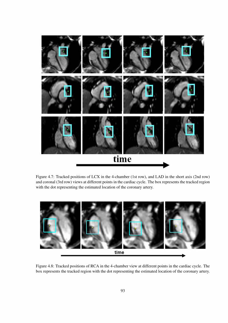
Figure 4.7: Tracked positions of LCX in the 4-chamber (1st row), and LAD in the short axis (2nd row)and coronal (3rd row) views at different points in the cardiac cycle. The box represents the tracked regionwith the dot representing the estimated location of the coronary artery.

Figure 4.8: Tracked positions of RCA in the 4-chamber view at different points in the cardiac cycle. Thebox represents the tracked region with the dot representing the estimated location of the coronary artery.

93

Figure 4.9: Tracked coronary motion in low resolution real-time images. The top (a) and bottom (b) rowscorrespond to 4-chamber and short axis views respectively. The left column shows the transformed heartcoordinate system (in gray) whereas the right column shows the transformed tracked coronary motionof LCX and RCA in 4-chamber and LDA in short-axis views. The transformed tracked coronary motionplot shows the X ′, Y ′ and Z′ motions.

94

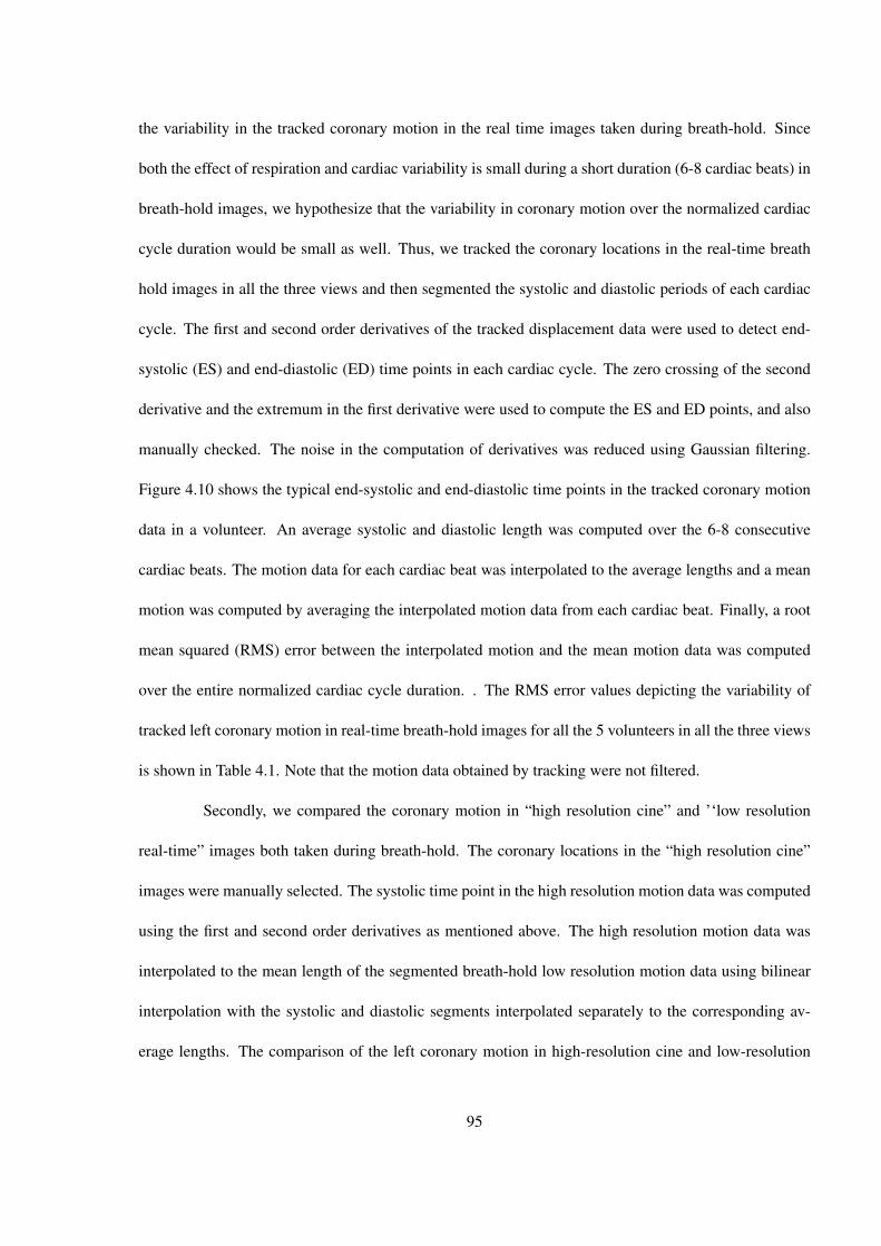
the variability in the tracked coronary motion in the real time images taken during breath-hold. Since

both the effect of respiration and cardiac variability is small during a short duration (6-8 cardiac beats) in

breath-hold images, we hypothesize that the variability in coronary motion over the normalized cardiac

cycle duration would be small as well. Thus, we tracked the coronary locations in the real-time breath

hold images in all the three views and then segmented the systolic and diastolic periods of each cardiac

cycle. The first and second order derivatives of the tracked displacement data were used to detect end-

systolic (ES) and end-diastolic (ED) time points in each cardiac cycle. The zero crossing of the second

derivative and the extremum in the first derivative were used to compute the ES and ED points, and also

manually checked. The noise in the computation of derivatives was reduced using Gaussian filtering.

Figure 4.10 shows the typical end-systolic and end-diastolic time points in the tracked coronary motion

data in a volunteer. An average systolic and diastolic length was computed over the 6-8 consecutive

cardiac beats. The motion data for each cardiac beat was interpolated to the average lengths and a mean

motion was computed by averaging the interpolated motion data from each cardiac beat. Finally, a root

mean squared (RMS) error between the interpolated motion and the mean motion data was computed

over the entire normalized cardiac cycle duration. . The RMS error values depicting the variability of

tracked left coronary motion in real-time breath-hold images for all the 5 volunteers in all the three views

is shown in Table 4.1. Note that the motion data obtained by tracking were not filtered.

Secondly, we compared the coronary motion in “high resolution cine” and ’‘low resolution

real-time” images both taken during breath-hold. The coronary locations in the “high resolution cine”

images were manually selected. The systolic time point in the high resolution motion data was computed

using the first and second order derivatives as mentioned above. The high resolution motion data was

interpolated to the mean length of the segmented breath-hold low resolution motion data using bilinear

interpolation with the systolic and diastolic segments interpolated separately to the corresponding av-

erage lengths. The comparison of the left coronary motion in high-resolution cine and low-resolution

95

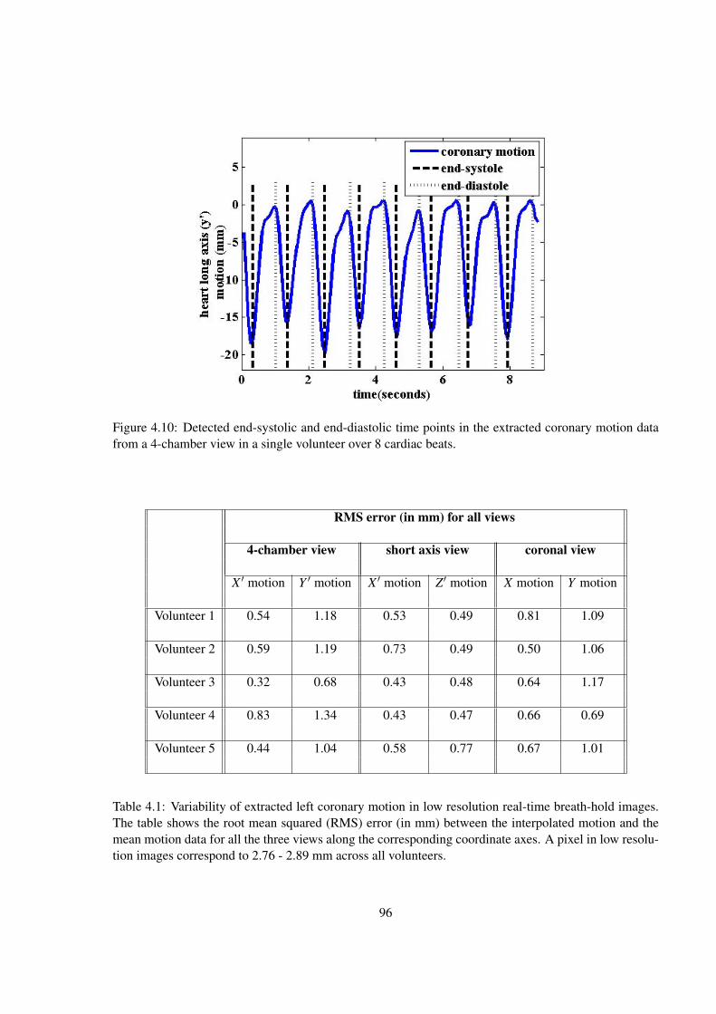
Figure 4.10: Detected end-systolic and end-diastolic time points in the extracted coronary motion datafrom a 4-chamber view in a single volunteer over 8 cardiac beats.

RMS error (in mm) for all views

4-chamber view short axis view coronal view

X ′ motion Y ′ motion X ′ motion Z′ motion X motion Y motion

Volunteer 1 0.54 1.18 0.53 0.49 0.81 1.09

Volunteer 2 0.59 1.19 0.73 0.49 0.50 1.06

Volunteer 3 0.32 0.68 0.43 0.48 0.64 1.17

Volunteer 4 0.83 1.34 0.43 0.47 0.66 0.69

Volunteer 5 0.44 1.04 0.58 0.77 0.67 1.01

Table 4.1: Variability of extracted left coronary motion in low resolution real-time breath-hold images.The table shows the root mean squared (RMS) error (in mm) between the interpolated motion and themean motion data for all the three views along the corresponding coordinate axes. A pixel in low resolu-tion images correspond to 2.76 - 2.89 mm across all volunteers.

96

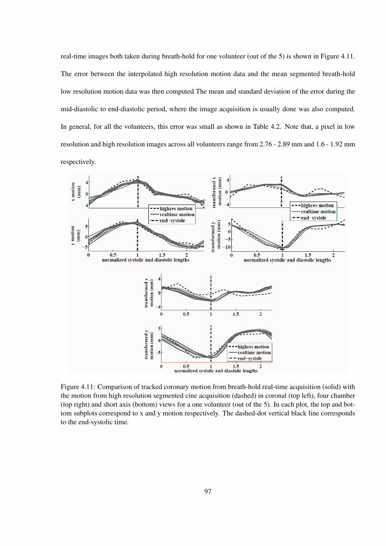
real-time images both taken during breath-hold for one volunteer (out of the 5) is shown in Figure 4.11.

The error between the interpolated high resolution motion data and the mean segmented breath-hold

low resolution motion data was then computed The mean and standard deviation of the error during the

mid-diastolic to end-diastolic period, where the image acquisition is usually done was also computed.

In general, for all the volunteers, this error was small as shown in Table 4.2. Note that, a pixel in low

resolution and high resolution images across all volunteers range from 2.76 - 2.89 mm and 1.6 - 1.92 mm

respectively.

Figure 4.11: Comparison of tracked coronary motion from breath-hold real-time acquisition (solid) withthe motion from high resolution segmented cine acquisition (dashed) in coronal (top left), four chamber(top right) and short axis (bottom) views for a one volunteer (out of the 5). In each plot, the top and bot-tom subplots correspond to x and y motion respectively. The dashed-dot vertical black line correspondsto the end-systolic time.

97

4.6 Heart Rate Variability

Since most HRV studies have focused on long term variability (24 hours for example), there

is little quantitative data indicating the magnitude of variability in short time spans used for cardiac MR

imaging [99, 100, 101]. We analyzed the heart rate variability using the tracked motion data for the

purpose of determining its impact on MRI quality (see the MR simulation section). The systolic and

diastolic time periods were calculated (as discussed in the previous section) and the variability (mean

and standard deviation) for both time periods was assessed for all 5 volunteers. Figure 4.12 shows the

heart rate variability in these volunteers. The mean systolic period over all volunteers was 380-400

milliseconds with a standard deviation of 48-62 milliseconds. The diastolic period on the other hand

had a much larger variability with a mean of 610-900 milliseconds and a standard deviation of 66-87

milliseconds as expected. The duration of the exam ranged from 10-39 minutes in the 5 subjects.

Error between high resolution and average lowresolution realtime tracked motion

4-chamber view short axis view coronal view

mean std dev mean std dev mean std dev(mm) (mm) (mm) (mm) (mm) (mm)

Volunteer 1 1.84 0.73 1.13 0.42 1.32 0.56

Volunteer 2 1.47 0.72 0.71 0.44 1.00 0.48

Volunteer 3 0.81 0.47 1.28 0.47 1.17 0.49

Volunteer 4 2.90 0.99 1.54 0.38 1.52 0.45

Volunteer 5 1.95 0.93 1.66 0.69 1.94 0.84

Table 4.2: Mean total error (in mm) between high resolution and average low resolution real-time trackedmotion. The error is computed during the second half of the diastolic period which is defined as theduration between the middle and end points of the diastolic period.

98

Figure 4.12: Variability in the diastolic and systolic periods in 5 volunteers. The duration of the examwas approximately 21, 15, 39, 11 and 10 minutes, respectively for the 5 volunteers. The error bars arethe standard deviation of each period.

4.7 MR Simulation

Figure 4.13: Flowchart describing the MR simulation analysis.

In order to determine the effect of cardiac motion variability on image quality prior to imple-

99

Figure 4.14: Acquisition window selection for adaptive (empty boxes) and fixed (filled boxes) triggerdelays for window width of 65 ms. The solid curve shows the x and y motion profiles (in cm). The dottedvertical lines depict the end-systolic time point. The fixed trigger delay acquisition window depictedby the duration between the two filled boxes is calculated from minimum velocity time point in thehigh resolution cine sequence. The adaptive trigger delay acquisition window depicted by the durationbetween the two empty boxes is computed on a beat-to-beat basis as the time point corresponding to theminimum velocity point in that cardiac cycle.

menting the method online on a scanner, we used motion data derived from human subjects combined

with simulation of the MR acquisition. This approach allowed us to combine realistic motion data and

variability into MR simulation data, and allows the exploration of a number of algorithms for selecting

the appropriate acquisition window and location for reducing motion artifacts. This approach is more

efficient and less costly for refining the adaptive algorithms than implementing variants online in the

scanner environment and acquiring live data. We used a synthetic image with simple structure that con-

tained two representative coronary arteries, one oriented through the image plane and the other in-plane,

each of them 4 mm in diameter. The coronary arteries are embedded in simulated myocardium which

is surrounded by simulated fat as shown in Figure 4.13. The flowchart in Figure 4.13 describes the MR

simulation analysis. A 2D segmented gradient echo imaging sequence was simulated (MATLAB, Math-

100

works Inc., Natick, MA) with the following parameters: in-plane resolution - 1mm, TE/TR/FL 8/15/20,

T1 fat 260ms, blood 100ms (simulating in-flow), myocardium 870ms. For each of the 5 subjects, the

coronary (RCA or LAD or LCX) motion data obtained from the tracking algorithm in each of the coro-

nal, short axis and four chamber views (see section 4.5) were fed to the simulation. The coronary phan-

tom underwent the extracted coronary motion while the segmented k-space acquisition was performed.

Respiratory motion was first removed from the coronary trajectories by filtering out the low frequency

respiratory component of the motion to reduce the analysis to cardiac motion only. We hypothesize that

in the presence of cardiac variability (with the respiration removed), the proposed adaptive trigger delay

acquisition window selection for each heartbeat would provide better cardiac motion compensation than

the standard approach of fixed trigger delay for all heartbeats. Since the number of heartbeats used in the

simulation is small, there is a chance that a single beat with large motion that falls in the center of k-space

will have a large impact on the motion artifacts on the reconstructed image. Thus we ran the simulation

on 10 sets of heartbeats for each case to remove bias. It is important to note that although we haven’t

implemented retrospective rejection of beats with large motion this can be easily incorporated in the pro-

posed method. The ideal fixed trigger delay was determined by locating the minimal velocity time period

of the coronary artery during mid-diastole in high resolution cine images acquired at the same location.

The RCA or LCX or LAD location in high resolution cine images was manually selected throughout the

cardiac cycle and then filtered using Savitzky-Golay filters. A moving window average approach with a

150 ms duration window was run on the coronary velocity (computed by finite difference method) and

the time point corresponding to the minimum was selected as the fixed trigger delay for all acquisition

window widths. It is important to note that previous methods [106, 112] choose either bulk cardiac or

myocardium motion for determining the optimal fixed trigger delay as compared to the actual coronary

motion as done in the present study. The adaptive trigger delay was determined by the time point of min-

imum velocity in the second half of each heartbeat on a beat-to-beat basis. The velocity was calculated

101

using the first order derivatives computed as mentioned in the tracking validation section. Although one

can argue that a moving window average approach similar to the one selected for estimating the fixed

trigger delay would be a better approach, we chose this simple approach due to its practicality and ease of

implementation for the planned online approach using prediction algorithms [113]. Acquisition window

widths of 65 ms, 100 ms, 150 ms and 200 ms were tested for each subject in each of the coronal, short

axis and four chamber views. Figure 4.14 shows 65 ms acquisition window selection for a few cardiac

cycles for both adaptive and fixed trigger delays. The number of lines in k-space per heartbeat was 3, 5,

7.6 and 10.75 for the acquisition window widths of 65, 100, 150 and 200 ms respectively. The CNR of

the coronary compared to background “myocardium”, and SNR of the coronary were computed in each

case. The CNR and SNR were computed as follows

SNR =Iavg−cor

σair

CNR =Iavg−cor− Iavg−myo

σair

(4.1)

where Iavg−cor and Iavg−myo are the average intensities in the coronary artery region and the myocardium

region surrounding the coronary artery and σair is the standard deviation of intensities in the air region.

As the motion applied to the synthetic image is in 2 dimensions, the curved coronary artery (see Figure

4.13) is used to discern the effect of in-plane motion and the circular coronary artery (see Figure 4.13)

depicts the effect of through plane motion. In the present analysis, the SNR and CNR values of only the

curved in plane coronary artery in the synthetic image is presented. We also computed the percent gain or

loss in SNR (SNRgl) of the adaptive delay method over the fixed delay method as SNRadaptive−SNR f ixedmin(SNRadaptive,SNR f ixed)

. For each view in all the subjects, an average SNRgl is computed over all the 10 simulation runs. Using

the average SNRgl we obtained the best and worst case results for each acquisition window across all the

volunteers.

The best and worst case image comparisons of fixed and adaptive trigger delay implementa-

tions for each acquisition window are shown in Figure 4.15. Even in the worst case scenario; the ghosting

102

due to motion in the adaptive delay case is comparable to that in fixed delay case for all acquisition win-

dows. In general, image quality degrades at longer acquisition windows highlighting that selection of

optimal window duration as well as location in the cardiac cycle is subject specific.

A three-way ANOVA analysis (with full interaction) was also performed on both SNR and

CNR values to determine the significance of the adaptive trigger delay approach over the fixed trigger

delay method for all the acquisition window widths, using acquisition window length, volunteer and

the trigger delay method used. The ANOVA analysis was followed by a pairwise comparison with

acquisition window length and trigger delay methods as factors to test whether the means for the two

trigger delay methods are statistically different for each acquisition window length.

The comparison of the CNR and SNR values computed on the reconstructed images between

the adaptive and fixed trigger delay approaches for both left and right coronary arteries is shown in Figure

4.16. For the left coronary artery, across all subjects, both CNR and SNR average values were greater in

the adaptive delay case than in the fixed delay case for all acquisition windows. Also, the 3-way ANOVA

analysis for both SNR and CNR showed that there was statistical significance (p < 0.0001) between the

means of the fixed and adaptive trigger delay methods. The statistical significance (p < 0.05) between the

means (for SNR and CNR) of the two methods for each acquisition window was shown by the pair-wise

comparison analysis. The incremental benefit of the adaptive trigger delay method in terms of the SNR

and CNR values is much lower for the right coronary artery as compared to the left coronary artery,

especially for larger acquisition window lengths. Based on our initial investigation, we believe this is

due to a more complex motion profile of the right coronary artery in some volunteers that renders the

simple minimum velocity point approach for computing adaptive trigger delay ineffective.

103

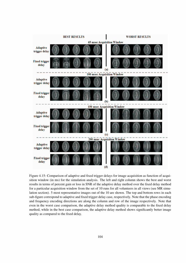
Figure 4.15: Comparison of adaptive and fixed trigger delays for image acquisition as function of acqui-sition window (in ms) for the simulation analysis. The left and right column shows the best and worstresults in terms of percent gain or loss in SNR of the adaptive delay method over the fixed delay methodfor a particular acquisition window from the set of 10 runs for all volunteers in all views (see MR simu-lation section). 5 most representative images out of the 10 are shown. The top and bottom rows in eachsub-figure correspond to adaptive and fixed trigger delay case, respectively. Note that the phase encodingand frequency encoding directions are along the column and row of the image respectively. Note thateven in the worst case comparison, the adaptive delay method quality is comparable to the fixed delaymethod, while in the best case comparison, the adaptive delay method shows significantly better imagequality as compared to the fixed delay.

104

Figure 4.16: SNR (left column) and CNR (right column) comparison between adaptive (dark gray) andfixed (light gray) trigger delays for different acquisition windows for left (a) and right (b) coronaryartery. Each plot is a box and whisker plot in MATLAB (Mathworks Inc.). The box has lines at the lowerquartile, median, and upper quartile values. The whiskers (dotted lines) are a function of inter-quartilerange. The pluses denote the outliers beyond the whisker range. One can note that as the acquisitionwindow increases, the incremental benefit of an adaptive delay is decreased.

105

4.8 Comparison of Diaphragm and Coronary Motion

In this part of study, we investigated the following two questions: 1) how well are the di-

aphragm motion and respiratory component of the coronary motion correlated? and 2) what is the extent

of error introduced by using the commonly adopted 0.6 as a conversion factor [2]. Although that em-

pirical factor is not used by all published studies, we selected it to demonstrate the effect of making any

fixed assumption. In order to compare motion we track the coronary location and the lung-diaphragm

interface in real-time coronal view images. Figure 4.17(top) shows the location of the left coronary artery

and the lung-diaphragm interface in a coronal view. The dots denote the center of the region indicated

by dark and light gray boxes that are used for tracking (see 4.5 section for details on the tracking al-

gorithm). A subset of the tracked profiles of both the coronary artery and the lung-diaphragm interface

for one volunteer are shown as well in Figure 4.17 (bottom). Also, the respiratory component of the

coronary motion extracted using Fourier filtering analysis is shown. The tracked motion profiles over a

much longer duration of time (≈ a minute) is shown in Figure 4.18.

The root mean squared (RMS) error between the estimated (0.6*lung-diaphragm interface)

and extracted respiratory component of coronary motion was computed during all the time points and

also during mid-diastolic end-expiratory phases where data acquisition usually is performed. The end-

expiratory phases were selected similar to the lung-diaphragm navigator acceptance window selec-

tion [73]. The mid-diastolic windows in end-expiratory cardiac cycles were selected manually based

on minimum velocity point in mid-diastolic part of the cardiac cycle. Figure 4.19 shows the bar plot of

the rms errors across all volunteers.

The total RMS error over all time points in the cardiac cycle ranged from 0.95 - 1.34 mm and

during the mid-diastolic end-expiratory phases ranged from 0.47 - 1.19 mm. It is important to note here

that the respiratory signals were made zero-mean before the error was computed as the offset because a

difference of means would artificially increase the error.

106

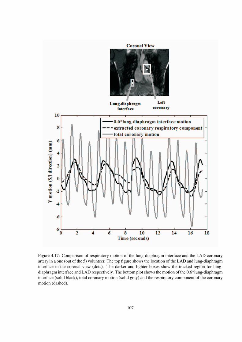
Figure 4.17: Comparison of respiratory motion of the lung-diaphragm interface and the LAD coronaryartery in a one (out of the 5) volunteer. The top figure shows the location of the LAD and lung-diaphragminterface in the coronal view (dots). The darker and lighter boxes show the tracked region for lung-diaphragm interface and LAD respectively. The bottom plot shows the motion of the 0.6*lung-diaphragminterface (solid black), total coronary motion (solid gray) and the respiratory component of the coronarymotion (dashed).

107

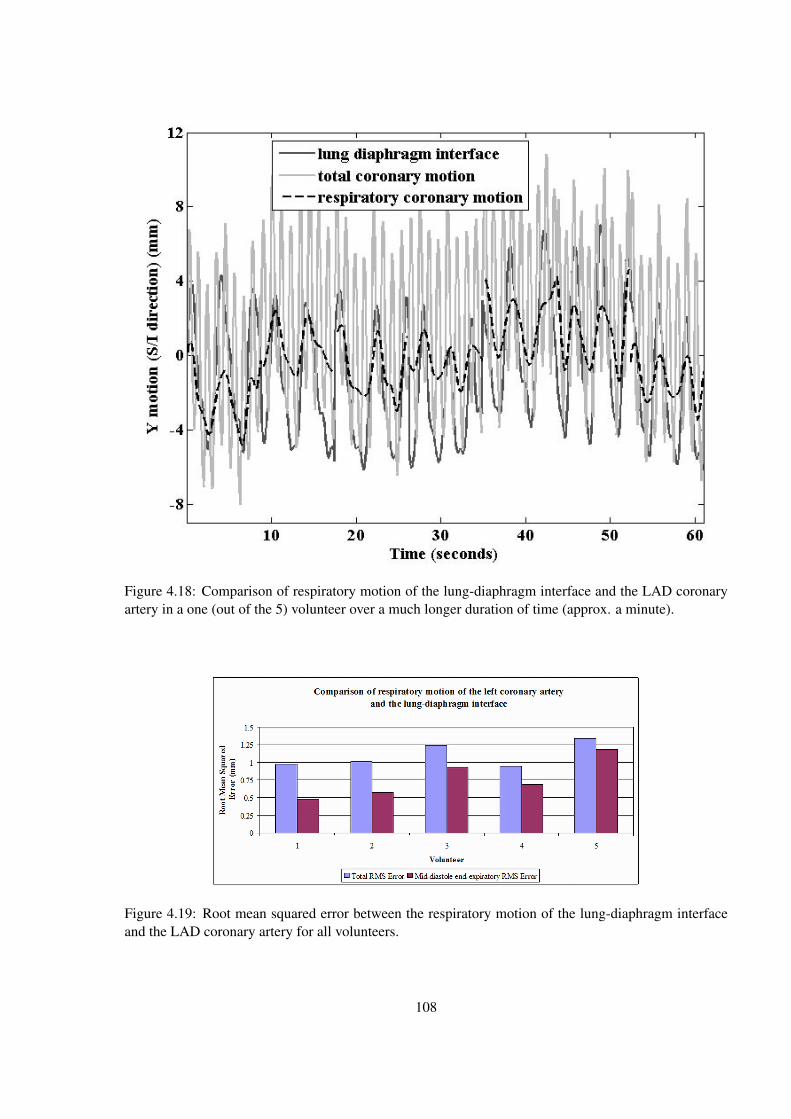
Figure 4.18: Comparison of respiratory motion of the lung-diaphragm interface and the LAD coronaryartery in a one (out of the 5) volunteer over a much longer duration of time (approx. a minute).

Figure 4.19: Root mean squared error between the respiratory motion of the lung-diaphragm interfaceand the LAD coronary artery for all volunteers.

108

4.9 User Interface (UI)

As a further step towards integrating the approach on an MR scanner, we have developed a real-

time tracking interface that allows for testing and validation of the proposed approach without significant

modifications to the scanner. In this section, we present our preliminary results from this system.

The tracking algorithm discussed in Section 4.5 was implemented in Visual C++. with a com-

putation time of less than 0.5 millisecond per image frame on a standard laptop. The UI was built around

the process flow of the tracking algorithm, which is as follows:

1. A set of images in the two orthogonal orientations of predominant coronary motion is acquired

over a few cardiac cycles.

2. A representative set of multiple templates is selected in these images for tracking (done offline).

3. The user selects the tracking parameters.

4. Online images in both the orientations are then acquired in which the coronary location is tracked

in real-time.

The interface was developed using RadBuilder (Siemens Corporate Research, Inc), a platform

for rapid application development. The RadBuilder framework is built on top of a family of open source

libraries (ITK, Open Inventor). As the proposed approach involves tracking in multiple views, the inter-

face allows for toggling between each view for tracking initialization. Figure 4.20 shows the screenshots

of the two toggled views of the UI. The bottom image shows the 4-chamber toggled view. The inter-

face allows for loading both real-time low resolution and high resolution cine images for the template

selection process. The user can view the selected templates and easily edit/modify selections. The track-

ing parameters can be selected from a task card. After selecting the templates and parameters, the user

switches to scanner mode to start tracking on live images from the scanner. The tracking result is overlaid

109

on the image and shown to the user. The interface also provides a toggled view to see the tracking results

in both views simultaneously as well (shown as the top image in Figure 4.20). The coronary tracking

interface runs on an independent workstation connected via ethernet to the scanner host computer. The

approach similar to that used in the IFE framework [114] is used for communication with the scanner to

obtain images and send slice updates.

4.9.1 Initial Testing and Results

The interface was first tested offline by tracking in pre-acquired sequences of 4-chamber and

short-axis images. The bottom image in Figure 4.20 shows a screenshot of LCX tracking in the 4-

chamber view. The online testing was done on a volunteer and a simple phantom consisting of two tubes

where the relative distance of tubes was changed to simulate non-rigid motion. The online testing was

done in each orientation separately. The scanning parameters were as follows: TrueFISP images with

TR/TE/FL=3.08/1.54/56, GRAPPA accel=2, in-plane resolution = 2.3mm, slice thickness = 12mm. The

screenshots from online testing for the phantom and a volunteer are shown in Figure 4.21. The tracking

accuracy was visually assessed and was found to be as accurate as the previous offline version of the

tracking algorithm.

4.10 Discussion and Conclusions

In this chapter, we have presented a subject-specific motion compensation approach for imag-

ing of the coronary arteries in MR. The proposed approach may reduce the effect of motion variability by

tracking of the location of the coronary artery on a beat-to-beat basis in real-time MR images in specific

slice orientations in which the coronary artery is known to have predominant motion. The extracted mo-

tion information can then be used to compensate for motion and guide high resolution data acquisition.

As the coronary motion is measured “directly”, the approach is inherently subject-specific and is suited

110

Figure 4.20: Screenshots of the coronary UI. The two screenshots show two (out of the four) toggledviews of the UI.

111

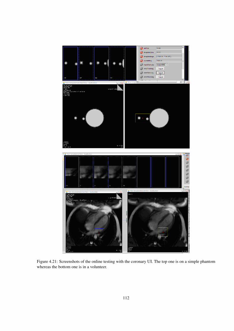
Figure 4.21: Screenshots of the online testing with the coronary UI. The top one is on a simple phantomwhereas the bottom one is in a volunteer.

112

to compensate for beat-to-beat variability in both cardiac and respiratory motion. Note that if motion of

different coronaries is dissimilar [82], the proposed approach will allow targeting of a particular coronary

segment if required. In the present study we hypothesized that:

1. Real-time imaging can be used to track the coronary arteries with sufficient accuracy. The low error

values presented in the tracking validation results demonstrated sub pixel tracking accuracy in low

resolution real-time images and showed good correlation between coronary motions in breath hold

low-resolution real-time and high-resolution cine images. To gauge the error values, a pixel in low

resolution and high resolution images across all volunteers corresponds to 2.76 - 2.89 mm and 1.6 -

1.92 mm respectively. Other factors of variability like the effect of respiration and the repeatability

of the cardiac position over heart beats are still present. Keeping in mind the variability in coronary

motion, manual coronary selection and tracking, the error values are small and within acceptable

limits. The interpolation of motion data is another source of error. The tracking results were

also assessed visually and were found to be in good agreement with the exception of occasional

misaligned frames in early diastole which is characterized by rapid motion. Also, the tracking

algorithm was able to handle long-term variations in appearance due to respiration. Although

in the presented work, the tracking was done offline in MATLAB (Mathworks Inc.), we have

implemented the tracking algorithm in C++ and the tracking computation time per image frame is

now less than half a millisecond on a standard laptop.

2. The variability in heart rate and cardiac motion significantly affect the image quality when fixed

acquisition periods are used. We have shown that there is a significant amount of variation in the

heart rate during the time spans used for cardiac MR imaging. The variability in diastolic period

is much larger than during the systolic period which is in agreement with prior work in heart rate

variability [103, 104]. As shown in Figure 4.15, motion artifacts are more pronounced when fixed

trigger delay is used resulting in low SNR and CNR values ( Figure 4.16). Thus, we conclude that

113

the image quality of the current MR methods for coronary imaging that use fixed trigger delays for

cardiac motion gating is limited in part due to the motion artifacts introduced by the variability in

cardiac cycles.

3. Beat-to-beat motion compensation can improve image quality We demonstrate that compensating

for the cardiac motion variability by adaptively choosing the trigger delay on a beat-to-beat basis

reduces the motion artifacts and hence improves the image quality ( Figure 4.15). This was done

by simulating imaging of a representative synthetic coronary artery that undergoes the motion

extracted from tracking the actual coronary artery in real-time MR images. For the left coronary

artery, the SNR and CNR for all the volunteers increased for different acquisition windows if

the trigger delay was chosen adaptively as compared to the fixed case ( Figure 4.16). The effect

was less pronounced for the right coronary artery. As mentioned in the results, we believe this

is due to the ineffectiveness of the simple minimal velocity approach for computing the adaptive

trigger delay in some volunteers. Presently, we are refining the algorithm to handle more complex

motion profiles for the adaptive trigger delay computation and anticipate that this would improve

results for the right coronary artery. The incremental benefit of the adaptive trigger delay was more

pronounced for the shorter acquisition windows as compared to the longer ones. This is important

as it has been shown that the duration of minimal motion in a cardiac cycle for patients is usually

small (order of 50-100ms) [82]. Although in the present work, the adaptive trigger delay (or the

minimal motion time point) was computed offline, the predictive modeling techniques [113] can

be easily incorporated into the framework for the online implementation.

4. Lung-diaphragm interface motion is insufficient to account for variability in respiratory motion of

the coronary arteries We have shown that although on average there is good correlation between

the respiratory component of coronary motion and lung-diaphragm interface motion, the variabil-

ity in the difference between the two is large suggesting that the diaphragm motion is insufficient to

114

completely compensate for respiratory motion of the coronary arteries. It is important to note that

the respiratory component of coronary motion only along superior/inferior direction was consid-

ered. The error would be much higher if components of respiratory motion along other directions

were considered as well.

Additonally, we have also presented an integrated system for real-time coronary motion track-

ing that will provide a basis for implementation of the proposed approach on the scanner. Although our

preliminary results are promising we recognize that the present study has a number of limitations.

1. There is a trade-off between the spatial and temporal resolutions of the real-time acquisition which

will also affect the coronary motion tracking accuracy. In the present work, we did not investigate

the selection of spatial and temporal resolutions and their effect on the tracking accuracy.

2. The method of choosing a fixed trigger delay can affect the image quality, and we have only

compared one method of selecting a fixed trigger delay.

3. A translational motion model is used and the motion is measured only in primary directions. Ac-

counting for motion components in other directions and using a more complex motion model could

make an impact in some subjects.

4. The simulation study is limited to a 2D gradient echo approach whereas most commonly used

acquisitions are 3D for coronary MRA. Also, slice following is not included in simulating the

acquisitions.

5. We have not yet addressed the need to account for motion that would occur between the end of the

tracking phase of the acquisition and the high resolution imaging phase, nor have we integrated

the tracking algorithm into the scanner yet.

6. In the present work, we have not addressed the issue of optimal acquisition window duration and

115

have assumed it is selected by the user and is fixed throughout the image acquisition. Varying

acquisition window duration on a beat to beat basis may provide additional benefit.

116

Chapter 5

Improved Motion Compensation in

Cardiac Valve MR Imaging

5.1 Introduction

Cardiac valves are small, rapidly moving cardiac structures that maintain unidirectional blood

flow in the heart. There are four cardiac valves in the heart as shown in Figure 5.1 - mitral, tricuspid,

aortic and pulmonic. The mitral and tricuspid valves, referred to as atrioventricular (AV) valves lie

between the atria and the ventricles. In a normal heart, these valves allow only forward flow from the

atria to the ventricles and prevent any flow backward into the atria. The aortic and pulmonic valves on

the other hand are referred to as the ventriculoarterial (VA) valves and lie between the ventricles and the

major vessels leaving the heart, the aorta and pulmonary artery respectively. These valves, in a healthy

heart only permit flow into the vessels from the ventricles and prevent blood from flowing back into the

ventricles.

The heart valves can get diseased (and dysfunctional) in mainly two ways, a valvular stenosis

and valvular regurgitation. In valvular stenosis, there is narrowing, stiffening or thickening of the valve

117

Figure 5.1: Cardiac valves in the heart. The left image is a slice through the long axis of the heart. Theimage was taken from www.lifeisnow.com.

leaflets, thereby compromising the blood flow through the valve. Alternatively, sometimes the valve

becomes leaky and does not close tightly, which can cause some blood to leak backwards across the

valve. This condition is known as valvular regurgitation or insufficiency. Both these conditions cause

the heart to work harder in order to maintain normal blood flow to the body, which can eventually lead

to heart failure.

Although the incidence of cardiac-valvular diseases in US is relatively low compared to CAD,

it does cause considerable morbidity and mortality [11]. Additionally, the number of valve-related surg-

eries and congenital heart valve disease cases is significantly large (≈ 300,000) [11]. To fully charac-

terize the valvular lesions in patients, in particular the ones undergoing surgical interventions, not only

the valve morphology and flow needs to be quantified, but also the hemodynamic response of the heart

needs to be evaluated, especially ventricular impairment.

118

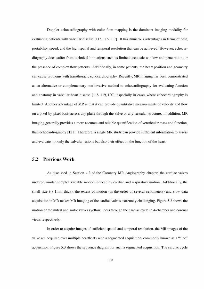
Doppler echocardiography with color flow mapping is the dominant imaging modality for

evaluating patients with valvular disease [115, 116, 117]. It has numerous advantages in terms of cost,

portability, speed, and the high spatial and temporal resolution that can be achieved. However, echocar-

diography does suffer from technical limitations such as limited accoustic window and penetration, or

the presence of complex flow patterns. Additionally, in some patients, the heart position and geometry

can cause problems with transthoracic echocardiography. Recently, MR imaging has been demonstrated

as an alternative or complementary non-invasive method to echocardiography for evaluating function

and anatomy in valvular heart disease [118, 119, 120], especially in cases where echocardiography is

limited. Another advantage of MR is that it can provide quantitative measurements of velocity and flow

on a pixel-by-pixel basis across any plane through the valve or any vascular structure. In addition, MR

imaging generally provides a more accurate and reliable quantification of ventricular mass and function,

than echocardiography [121]. Therefore, a single MR study can provide sufficient information to assess

and evaluate not only the valvular lesions but also their effect on the function of the heart.

5.2 Previous Work

As discussed in Section 4.2 of the Coronary MR Angiography chapter, the cardiac valves

undergo similar complex variable motion induced by cardiac and respiratory motion. Additionally, the

small size (≈ 1mm thick), the extent of motion (in the order of several centimeters) and slow data

acquisition in MR makes MR imaging of the cardiac valves extremely challenging. Figure 5.2 shows the

motion of the mitral and aortic valves (yellow lines) through the cardiac cycle in 4-chamber and coronal

views respectively.

In order to acquire images of sufficient spatial and temporal resolution, the MR images of the

valve are acquired over multiple heartbeats with a segmented acquisition, commonly known as a “cine”

acquisition. Figure 5.3 shows the sequence diagram for such a segmented acquisition. The cardiac cycle

119

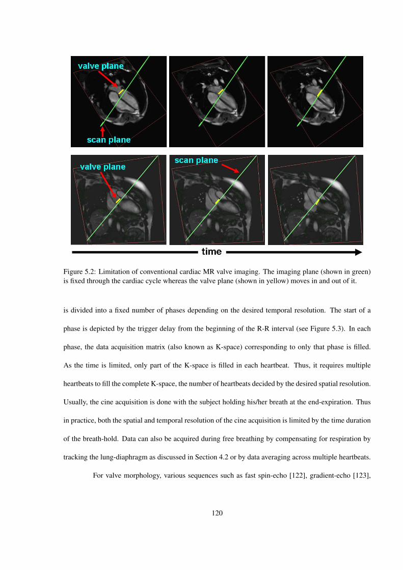
Figure 5.2: Limitation of conventional cardiac MR valve imaging. The imaging plane (shown in green)is fixed through the cardiac cycle whereas the valve plane (shown in yellow) moves in and out of it.

is divided into a fixed number of phases depending on the desired temporal resolution. The start of a

phase is depicted by the trigger delay from the beginning of the R-R interval (see Figure 5.3). In each

phase, the data acquisition matrix (also known as K-space) corresponding to only that phase is filled.

As the time is limited, only part of the K-space is filled in each heartbeat. Thus, it requires multiple

heartbeats to fill the complete K-space, the number of heartbeats decided by the desired spatial resolution.

Usually, the cine acquisition is done with the subject holding his/her breath at the end-expiration. Thus

in practice, both the spatial and temporal resolution of the cine acquisition is limited by the time duration

of the breath-hold. Data can also be acquired during free breathing by compensating for respiration by

tracking the lung-diaphragm as discussed in Section 4.2 or by data averaging across multiple heartbeats.

For valve morphology, various sequences such as fast spin-echo [122], gradient-echo [123],

120

Figure 5.3: Sequence diagram of a cine segmented acquisition. Images throughout the cardiac cycle areacquired. Each image (or its corresponding k-space data) is acquired over multiple heart beats.

121

and recently developed steady-state imaging [124,125] have been used with each having their advantages

and disadvantages. The most popular technique for measurement of flow is phase-contrast MR imaging,

also known as phase-shift or VENC (velocity-encoded) MR imaging. The basic principle exploited is

the fact that the phase shift of the MR signal of the blood flowing along a magnetic field gradient is

proportional to the blood flow velocity. Several methods over the last decade [126,127,128] have shown

the efficacy of phase-contrast MR sequence for quantitative flow measurement in aortic and mitral valves.

These methods usually select a single slice containing the valve of interest, that is imaged

throughout the cardiac cycle. The significant motion of the valve planes (max motion ≈ 10-15 mm)

through the cardiac cycle moves it in and out of the imaging slice (see Figure 5.2), thereby sometimes

providing inaccurate measurements and poor visualization. Recently, [129] proposed the use of MR

tagging to estimate the valve plane through the cardiac cycle offline during a pre-scan, and then acquiring

the data by adaptively moving the slice at different time points in the cardiac cycle with the motion

estimated during the pre-scan. MR tagging is used as a way of labeling such that only the signal from the

tissue in the valve plane shows up (see Figure 5.4). The approach was used to demonstrate improvement

in velocity measurements in patients with aortic and mitral regurgitation [130]. The valve plane was

tracked in one view i.e. coronal or 4-chamber view for aortic or mitral valve respectively. Dowsey

et al. [131] further extended the approach by tracking in two orthogonal views for the aortic valve for

improved valve visualization.

Although these methods showed improvements in flow measurements and visualization, they

suffered from the disadvantage that tags fade with time, thereby making the estimation difficult in later

parts of the cardiac cycle as shown in Figure 5.4. Additionally, for some valves, with tagging, it is

difficult to get enough signal from the tissue in the valve plane. Figure 5.5 shows the case for mitral valve

where the tagging slice was picked basal to the valve plane to get enough signal. Here, the underlying

assumption is that the motion of the tagged basal plane is same as the valve plane, which is generally not

122

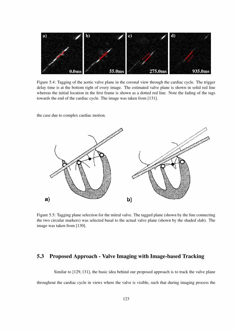
Figure 5.4: Tagging of the aortic valve plane in the coronal view through the cardiac cycle. The triggerdelay time is at the bottom right of every image. The estimated valve plane is shown in solid red linewhereas the initial location in the first frame is shown as a dotted red line. Note the fading of the tagstowards the end of the cardiac cycle. The image was taken from [131].

the case due to complex cardiac motion.

Figure 5.5: Tagging plane selection for the mitral valve. The tagged plane (shown by the line connectingthe two circular markers) was selected basal to the actual valve plane (shown by the shaded slab). Theimage was taken from [130].

5.3 Proposed Approach - Valve Imaging with Image-based Tracking

Similar to [129, 131], the basic idea behind our proposed approach is to track the valve plane

throughout the cardiac cycle in views where the valve is visible, such that during imaging process the

123

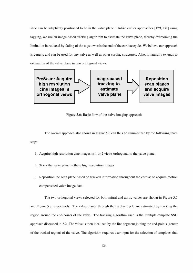
slice can be adaptively positioned to be in the valve plane. Unlike earlier approaches [129, 131] using

tagging, we use an image-based tracking algorithm to estimate the valve plane, thereby overcoming the

limitation introduced by fading of the tags towards the end of the cardiac cycle. We believe our approach

is generic and can be used for any valve as well as other cardiac structures. Also, it naturally extends to

estimation of the valve plane in two orthogonal views.

Figure 5.6: Basic flow of the valve imaging approach

The overall approach also shown in Figure 5.6 can thus be summarized by the following three

steps:

1. Acquire high resolution cine images in 1 or 2 views orthogonal to the valve plane.

2. Track the valve plane in these high resolution images.

3. Reposition the scan plane based on tracked information throughout the cardiac to acquire motion

compensated valve image data.

The two orthogonal views selected for both mitral and aortic valves are shown in Figure 5.7

and Figure 5.8 respectively. The valve planes through the cardiac cycle are estimated by tracking the

region around the end-points of the valve. The tracking algorithm used is the multiple-template SSD

approach discussed in 2.2. The valve is then localized by the line segment joining the end-points (center

of the tracked region) of the valve. The algorithm requires user input for the selection of templates that

124

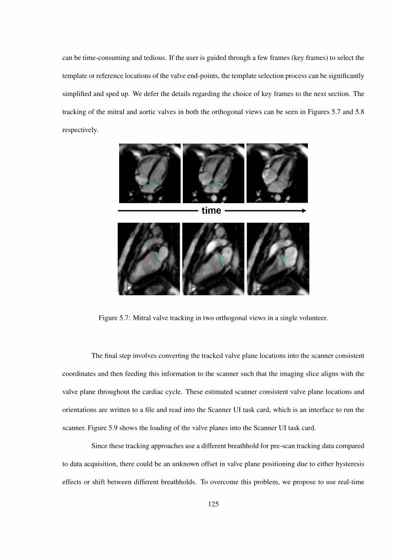
can be time-consuming and tedious. If the user is guided through a few frames (key frames) to select the

template or reference locations of the valve end-points, the template selection process can be significantly

simplified and sped up. We defer the details regarding the choice of key frames to the next section. The

tracking of the mitral and aortic valves in both the orthogonal views can be seen in Figures 5.7 and 5.8

respectively.

Figure 5.7: Mitral valve tracking in two orthogonal views in a single volunteer.

The final step involves converting the tracked valve plane locations into the scanner consistent

coordinates and then feeding this information to the scanner such that the imaging slice aligns with the

valve plane throughout the cardiac cycle. These estimated scanner consistent valve plane locations and

orientations are written to a file and read into the Scanner UI task card, which is an interface to run the

scanner. Figure 5.9 shows the loading of the valve planes into the Scanner UI task card.

Since these tracking approaches use a different breathhold for pre-scan tracking data compared

to data acquisition, there could be an unknown offset in valve plane positioning due to either hysteresis

effects or shift between different breathholds. To overcome this problem, we propose to use real-time

125

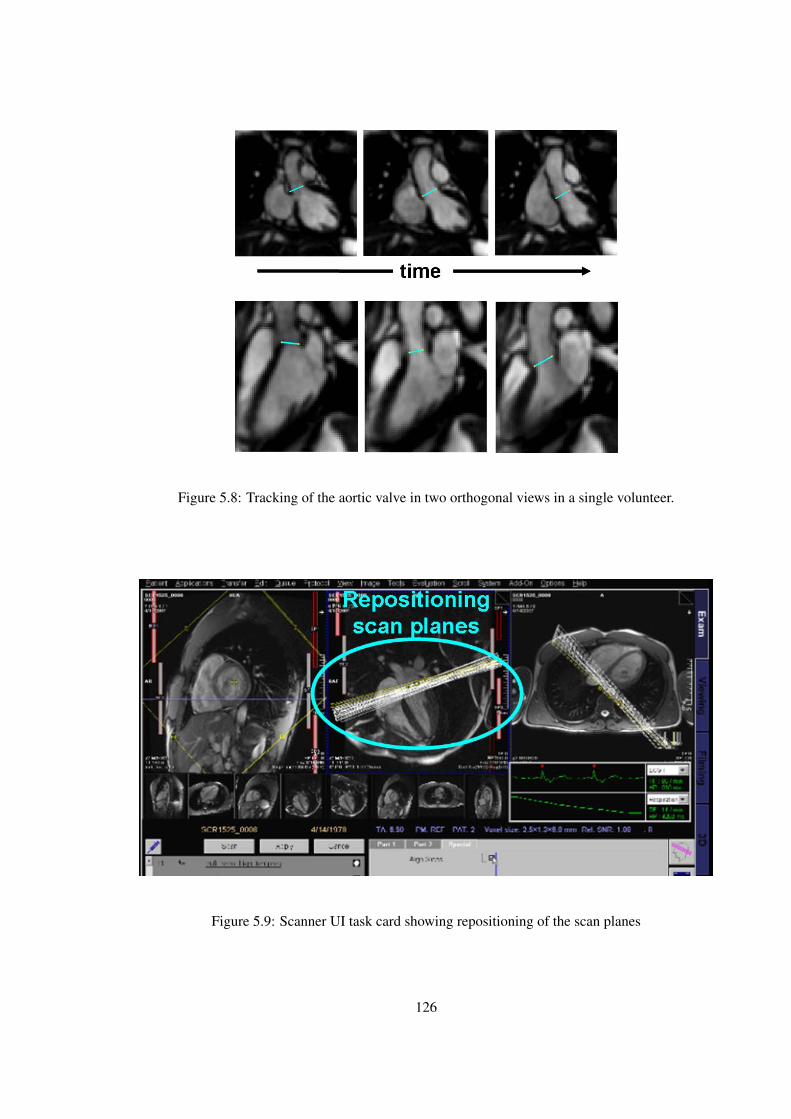
Figure 5.8: Tracking of the aortic valve in two orthogonal views in a single volunteer.

Figure 5.9: Scanner UI task card showing repositioning of the scan planes

126

tracking in one or two breathholds before switching to the data acquisition to correct for this offset.

Additionally, with MR imaging getting faster every day [108, 109], in future, the pre-scan step can

be replaced by a real-time acquisition and online feedback similar to the coronary imaging approach

discussed in the previous chapter (see Section 4.3).

Thus, we present the feasibility of tracking the valve in low resolution real time images. The

acquisition of the the low resolution images is discussed in Section 4.4. Again, we track the region

around the end-points of the valve using the multiple-template tracking algorithm discussed in 2.2. The

template selection was similar to that used for coronary artery tracking (see Section 4.5). Figure 5.10

shows the tracked mitral and aortic valve planes in low-resolution images in 4-chamber and coronal

views respectively. The tracking accuracy in real-time images was assessed visually and were found to

be in good agreement.

5.4 Validation and Experiments

In this section, we present two validation studies - the first one to validate the image-based

tracking and the second one to compare the proposed valve imaging approach using image-based tracking

with the conventional fixed plane approach.

5.4.1 Study I - Tracking Validation

In this section, we validate the valve tracking against manual selection in the high-resolution

images. We restrict ourselves to aortic and mitral valves in one view i.e. coronal and 4-chamber views

respectively. The high resolution cine images in this study were acquired in 5 volunteers. The details

on the parameters can be found in Section 4.4. As mentioned in the previous section, we track the end-

points of the valve to estimate the valve plane using a semi-automatic algorithm requiring user input for

the selection of templates. In order to speed-up the template selection, the user is guided through the

127

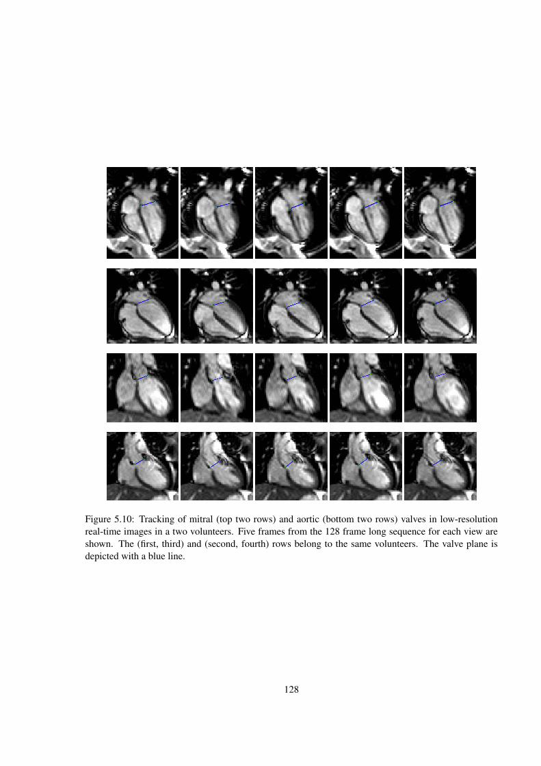
Figure 5.10: Tracking of mitral (top two rows) and aortic (bottom two rows) valves in low-resolutionreal-time images in a two volunteers. Five frames from the 128 frame long sequence for each view areshown. The (first, third) and (second, fourth) rows belong to the same volunteers. The valve plane isdepicted with a blue line.

128

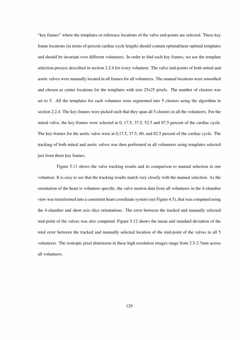
“key frames” where the templates or reference locations of the valve end-points are selected. These key

frame locations (in terms of percent cardiac cycle length) should contain optimal/near optimal templates

and should be invariant over different volunteers. In order to find such key frames, we use the template

selection process described in section 2.2.4 for every volunteer. The valve end-points of both mitral and

aortic valves were manually located in all frames for all volunteers. The manual locations were smoothed

and chosen as center locations for the templates with size 25x25 pixels. The number of clusters was

set to 5. All the templates for each volunteer were segmented into 5 clusters using the algorithm in

section 2.2.4. The key-frames were picked such that they span all 5 clusters in all the volunteers. For the

mitral valve, the key-frames were selected at 0, 17.5, 37.5, 52.5 and 87.5 percent of the cardiac cycle.

The key-frames for the aortic valve were at 0,17.5, 37.5, 60, and 82.5 percent of the cardiac cycle. The

tracking of both mitral and aortic valves was then performed in all volunteers using templates selected

just from these key frames.

Figure 5.11 shows the valve tracking results and its comparison to manual selection in one

volunteer. It is easy to see that the tracking results match very closely with the manual selection. As the

orientation of the heart is volunteer-specific, the valve motion data from all volunteers in the 4-chamber

view was transformed into a consistent heart coordinate system (see Figure 4.5), that was computed using

the 4-chamber and short axis slice orientations. The error between the tracked and manually selected

mid-point of the valves was also computed. Figure 5.12 shows the mean and standard deviation of the

total error between the tracked and manually selected location of the mid-point of the valves in all 5

volunteers. The isotropic pixel dimension in these high resolution images range from 2.5-2.7mm across

all volunteers.

129

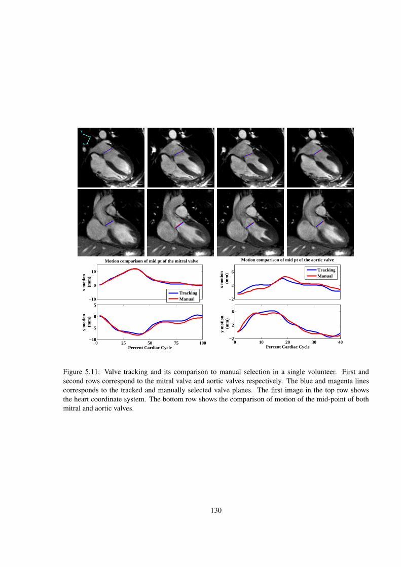
X

Y

−10

0

10

Motion comparison of mid pt of the mitral valve

x m

otio

n (m

m)

TrackingManual

0 25 50 75 100−10

−5

0

5

Percent Cardiac Cycle

y m

otio

n (m

m)

−2

2

6

Motion comparison of mid pt of the aortic valve

x m

otio

n (

mm

)

TrackingManual

0 10 20 30 40−2

2

6

Percent Cardiac Cycle

y m

otio

n (m

m)

Figure 5.11: Valve tracking and its comparison to manual selection in a single volunteer. First andsecond rows correspond to the mitral valve and aortic valves respectively. The blue and magenta linescorresponds to the tracked and manually selected valve planes. The first image in the top row showsthe heart coordinate system. The bottom row shows the comparison of motion of the mid-point of bothmitral and aortic valves.

130

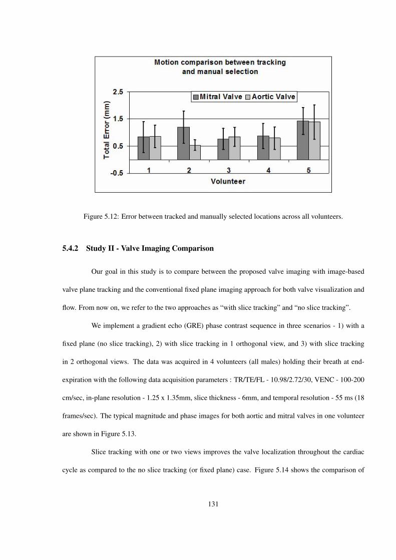
Figure 5.12: Error between tracked and manually selected locations across all volunteers.

5.4.2 Study II - Valve Imaging Comparison

Our goal in this study is to compare between the proposed valve imaging with image-based

valve plane tracking and the conventional fixed plane imaging approach for both valve visualization and

flow. From now on, we refer to the two approaches as “with slice tracking” and “no slice tracking”.

We implement a gradient echo (GRE) phase contrast sequence in three scenarios - 1) with a

fixed plane (no slice tracking), 2) with slice tracking in 1 orthogonal view, and 3) with slice tracking

in 2 orthogonal views. The data was acquired in 4 volunteers (all males) holding their breath at end-

expiration with the following data acquisition parameters : TR/TE/FL - 10.98/2.72/30, VENC - 100-200

cm/sec, in-plane resolution - 1.25 x 1.35mm, slice thickness - 6mm, and temporal resolution - 55 ms (18

frames/sec). The typical magnitude and phase images for both aortic and mitral valves in one volunteer

are shown in Figure 5.13.

Slice tracking with one or two views improves the valve localization throughout the cardiac

cycle as compared to the no slice tracking (or fixed plane) case. Figure 5.14 shows the comparison of

131

Figure 5.13: Magnitude and phase images for aortic (top row) and mitral valve (bottom row) when thecorresponding valves are open. The left and right column show magnitude and phase images respectively.The circle denotes the valve location.

132

the magnitude images of the aortic valve for a single volunteer. Better localization of the valve with slice

tracking is evident as the valve leaflets are visible throughout the cardiac cycle. Improved localization of

the mitral valve can also be seen in the comparison shown in in Figure 5.15. It is easy to see that the area

of the mitral valve (oval shape) is more consistent with slice tracking incorporated.

Figure 5.14: Comparison of the aortic valve visualization between with and without slice tracking. Threeframes in the cardiac cycle are shown. The location of the valve is indicated by the green circle. The first,second and third columns correspond to no slice tracking, slice tracking with 1 view and slice trackingwith 2 views respectively.

We also performed the flow analysis in the Syngo Argus (Siemens Inc.) flow tool in all the three

cases. This was done by first drawing a region of interest (ROI) around the valve in the phase images

133

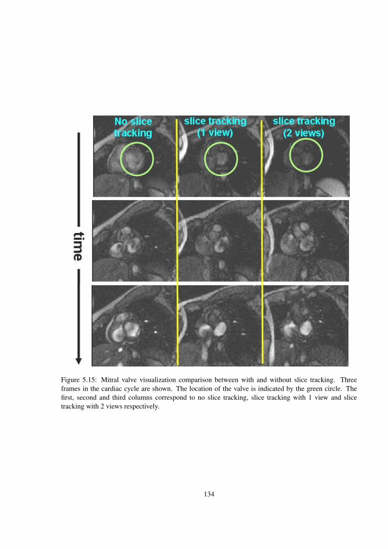
Figure 5.15: Mitral valve visualization comparison between with and without slice tracking. Threeframes in the cardiac cycle are shown. The location of the valve is indicated by the green circle. Thefirst, second and third columns correspond to no slice tracking, slice tracking with 1 view and slicetracking with 2 views respectively.

134

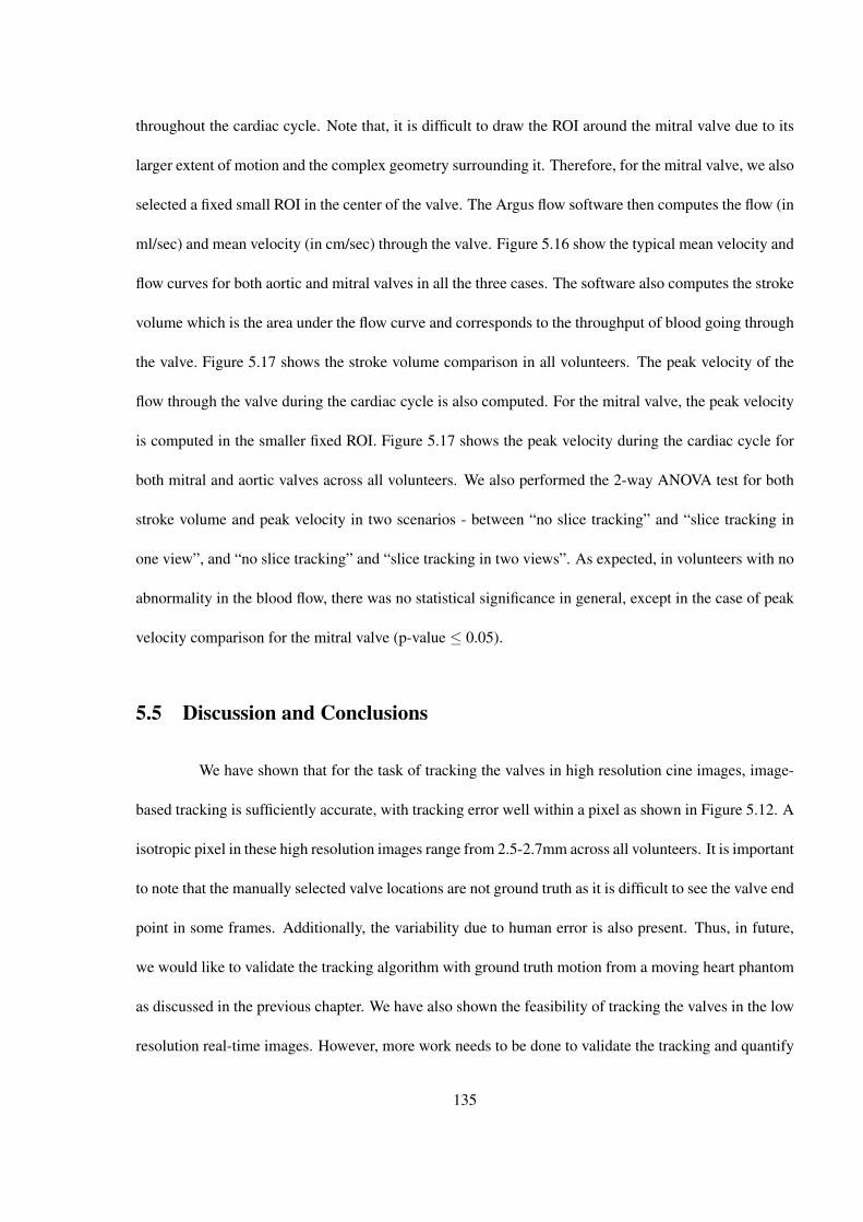
throughout the cardiac cycle. Note that, it is difficult to draw the ROI around the mitral valve due to its

larger extent of motion and the complex geometry surrounding it. Therefore, for the mitral valve, we also

selected a fixed small ROI in the center of the valve. The Argus flow software then computes the flow (in

ml/sec) and mean velocity (in cm/sec) through the valve. Figure 5.16 show the typical mean velocity and

flow curves for both aortic and mitral valves in all the three cases. The software also computes the stroke

volume which is the area under the flow curve and corresponds to the throughput of blood going through

the valve. Figure 5.17 shows the stroke volume comparison in all volunteers. The peak velocity of the

flow through the valve during the cardiac cycle is also computed. For the mitral valve, the peak velocity

is computed in the smaller fixed ROI. Figure 5.17 shows the peak velocity during the cardiac cycle for

both mitral and aortic valves across all volunteers. We also performed the 2-way ANOVA test for both

stroke volume and peak velocity in two scenarios - between “no slice tracking” and “slice tracking in

one view”, and “no slice tracking” and “slice tracking in two views”. As expected, in volunteers with no

abnormality in the blood flow, there was no statistical significance in general, except in the case of peak

velocity comparison for the mitral valve (p-value ≤ 0.05).

5.5 Discussion and Conclusions

We have shown that for the task of tracking the valves in high resolution cine images, image-

based tracking is sufficiently accurate, with tracking error well within a pixel as shown in Figure 5.12. A

isotropic pixel in these high resolution images range from 2.5-2.7mm across all volunteers. It is important

to note that the manually selected valve locations are not ground truth as it is difficult to see the valve end

point in some frames. Additionally, the variability due to human error is also present. Thus, in future,

we would like to validate the tracking algorithm with ground truth motion from a moving heart phantom

as discussed in the previous chapter. We have also shown the feasibility of tracking the valves in the low

resolution real-time images. However, more work needs to be done to validate the tracking and quantify

135

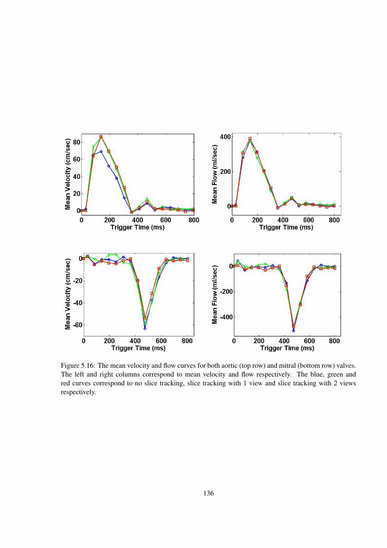
Figure 5.16: The mean velocity and flow curves for both aortic (top row) and mitral (bottom row) valves.The left and right columns correspond to mean velocity and flow respectively. The blue, green andred curves correspond to no slice tracking, slice tracking with 1 view and slice tracking with 2 viewsrespectively.

136

Figure 5.17: Stoke volume and peak veloctiy comparisons for flow measurements with and without slicetracking. The first and second rows correspond to aortic and mitral valves, whereas the left and rightcolumns correspond to peak velocity and stroke volume respectively. The legend is at the bottom.

137

the tracking accuracy.

In our preliminary study in normal volunteers, we have shown the implementation of valve

imaging with slice tracking for improved valve localization. The valve is visible throughout the cardiac

cycle with the incorporation of slice tracking as shown in Figures 5.14 and 5.15 . We did not notice much

difference between the two cases of slice tracking with one and two views. Additionally, we wish to note

that the image contrast in the slice tracking images is poor compared to the one without slice tracking

as we did not focus on optimizing the MR imaging sequence for image contrast. The flow analysis in

volunteers with normal blood flow did not show any statistical difference with slice tracking. Although,

the peak velocity comparison for the mitral valve turned out to be significant (p-value ≤ 0.05), we need

a much larger study to draw any conclusions.

As this is a preliminary study, there are some limitations that need to be addressed in future for

larger studies to draw any meaningful conclusions.

1. The mitral valve curves in Figure 5.16 do not have the “A-wave” [120], that corresponds to atrial

contraction and is towards the end of the cardiac cycle. As the data was acquired at a low temporal

resolution, this restricted the data acquisition towards the end of the cardiac cycle owing to pos-

sible heart rate changes during the acquisition. We plan to address this problem in the future by

acquiring data at a higher temporal resolution under free-breathing with respiration compensation.

2. In a normal heart, the stroke volume through the aortic and mitral valve should be same because

the cardiac input and output are identical. Note that in Figure 5.17, the mitral stroke volume is

lower than the aortic stroke volume. This is again due to missing “A-wave” mentioned earlier.

3. As discussed in the last paragraph, the MR imaging needs to be optimized for contrast (CNR) and

signal intensity (SNR) for better morphological images.

4. In the present study, we did not account for heart-rate change between the pre-scan and data ac-

138

quisition. Interpolation of valve planes can be used to address this issue.

We believe that the flow analysis with the slice tracking incorporated would be beneficial in

patients, especially the ones with abnormal flow patterns as shown by [130]. Thus, for future work, we

would like to further evaluate our approach on patients with valve regurgitation and/or stenosis condi-

tions.

To summarize, in this chapter, we have shown that the image-based tracking is a viable alter-

native to tagging approaches for improved motion compensation in valve MR imaging. The image-based

tracking is a more general approach compared to tagging and can be easily applied to any valve or car-

diac structure. Also, it overcomes the limitations of valve plane estimation towards the end of the cardiac

cycle due to tag fading.

139

Chapter 6

Conclusions and Future Work

6.1 Tracking Methods

The work described in this thesis contributes towards the goal of unifying and optimizing

visual tracking. With the abundance of tracking algorithms developed over the years, the choice of

tracking methods for a particular application has significantly increased, but it is generally not clear

what is the best algorithm to use. Most of the time, there is no single algorithm in a particular genre

that is optimal and usually a combination of algorithms is the best solution. For example, for tracking

an object with homogenous region and texture, intuitively a combination of feature and region based

algorithms complimenting each other would yield more accurate and robust tracking than using either

one individually. Additionally, there is no standard way to compare different algorithms to decide which

one is a better choice.

We believe the kernel-weighted histograms and their extensions described in Chapter 2 provide

a number of unifying insights into the general form and structure of visual tracking problems. Kernel-

based tracking methods forge a link between the two “extremes” in the spectrum of tracking algorithms,

namely blob tracking and template tracking. The SSD formulation and its extension to multiple ker-

nels developed in Chapter 2 allows for both faster convergence and easier insights into the underlying

140

connection between the two. Additionally, there is a fundamental relationship between the structure of

histograms for detecting and estimating target motion, and the spatial structure of the target itself. At one

extreme, a simple circularly symmetric kernel places few constraints on target motion, but in the limit, as

more and more kernels are added, the spatial structure of the target becomes more and more constrained.

Multiple kernels also naturally extend towards tracking complex motions or certain attributes of the tar-

get. Presently, we are continuing to develop insights into more challenging tracking problems. For

example, it is not yet clear how to properly adapt the histogram structure over time to adapt to changing

illumination, changing target appearance, or occlusion.

Traditional kernel-based approaches choose the kernel parameters in an ad-hoc fashion and

use the same kernel for all the image projections, thereby leading to sub-optimal tracking and even

tracking failure in some cases. Thus, we have presented a principled approach for optimizing the kernel

parameters (both scale and location) for a specific target. The optimizations performed either in a numer-

ical fashion or using faster approximations show improvements over both traditional kernel-based and

template-based SSD methods. The overall approach is general and can be used for not only optimizing

but also comparing other tracking methods.

The methods as described in Chapter 3 can be easily extended to choose multiple kernels in

multiple features spaces by extending the developed heuristics. However, the problem of creating a well-

developed theory and good approximations to evaluate multiple kernels operating in multiple feature

spaces remains an open problem, and one we are actively pursuing. For example, it is not clear how to

pick multiple kernels to reduce the overall tracking error. Likewise, approximations should be efficiently

computable to ensure that the optimization process can be carried out quickly on a per-target basis. This

is also a topic of current consideration.

In some cases, for example in cardiac MR images, a single template is not sufficient for track-

ing. Furthermore, the deformations are large and unmodelled, thereby ruling out kernel-based tracking

141

methods as well that handle small local deformations. Thus, we have presented a multiple template-based

tracking method that uses the templates itself, thereby providing a number of advantages over orthogo-

nal basis approaches [39]. The selection of a large number of multiple templates is time-consuming and

often error-prone. This can lead to underestimation of motion parameters. Thus, we present an algorithm

for the selection of a few optimal templates which emerges as a natural extension from the tracking al-

gorithm. To further improve the tracking accuracy, the approach also provides a framework for updating

multiple templates online and the use of a subset of templates, for the particular case of cardiac tracking.

The use of templates instead of orthogonal basis also allows the extension to the bidirectional gradient

optimization that improves the range of convergence. The efficacy of the tracking algorithm was shown

through the validation on MR images in different views of varying temporal and spatial resolution.

6.2 Motion Compensation in Cardiovascular MR

In the area cardiovascular MR, our goal is to develop methods to improve the speed, quality

and reliability of imaging cardiac structures. We have presented motion compensation approaches for

improved imaging of the coronary arteries and the cardiac valves and have demonstrated their effec-

tiveness. The underlying principle in both the approaches is the ability to track the cardiac structure in

motion affected MR images. The multiple-template algorithm mentioned earlier was used for tracking

these cardiac structures.

In coronary MR imaging, the 3D data acquisition, that can only be acquired during a small

window of minimal motion in the cardiac cycle places high requirements on motion compensation meth-

ods. To overcome limitations of the current approaches, we proposed a subject-specific “image-based

navigators” approach that performs beat-to-beat motion compensation by estimating the coronary motion

in low resolution real-time images and using the extracted motion to gate the data acquisition on a beat-

to-beat basis. The respiratory motion extracted from the tracked coronary motion can be used directly

142

for respiratory gating, thereby overcoming the limitations of the earlier approaches, where a surrogate

lung-diaphragm motion is used to compensate for respiratory component of the coronary motion. This

was demonstrated through significant error between the tracked respiratory component of the coronary

motion and the tracked lung-diaphragm motion across all volunteers. Additionally, as the approach mea-

sures coronary motion directly, it can handle short-term and long-term variability in coronary motion. We

have presented the feasibility of the approach by tracking the coronary motion reliably and accurately in

low resolution real-time MR images in different views across 5 volunteers. Through simulations, using

the tracked coronary motion in human volunteers, we have demonstrated that accounting for the motion

variability with adaptive window selection improves MR image quality. Therefore, we believe the pro-

posed subject-specific “image-based navigators” approach is feasible and will have potential advantage

over existing methods for coronary MR imaging by reducing the assumptions regarding motion of the

coronary arteries.

As the results from our current study are promising, we plan to integrate real-time coronary

tracking into the MR scanner and further evaluate the proposed approach for coronary MR imaging.

This will involve sequence modification that will allow switching between real-time tracking mode and

high resolution data acquisition mode. The real time capabilities of the Siemens Avanto/Espree scanners

allow real time decisions regarding keeping/discarding data and shifting of slice position, based on the

implementation of traditional navigators. Including application of preparation pulses (fat saturation, T2

prep, approach to steady state), the transition time is estimated to be approximately 50-70 ms. The tem-

poral resolution for a low resolution image acquisition is 50-70 ms (15-20 frames per second) and since

the approach requires acquisition of two orthogonal views, the total acquisition time for low resolution

real-time images is 100-140 ms. The computation time for the tracking algorithm is on the order of 1 ms

and prediction algorithms should be on the order of 10 ms [113] which is relatively small compared to the

image acquisition time and should not be a limiting factor in the online implementation. Since the mo-

143

tion information can be extracted after the image acquisition, it will be necessary to be able to accurately

predict the adaptive trigger delay at least 200 ms before the high resolution data acquisition. Thus, we

are investigating the development of online algorithms based on [113] for predicting the adaptive trigger

delay using tracked coronary motion history, as well as retrospective (next heartbeat) review of motion

and discarding of beats with motion that is dissimilar to that of an average cardiac cycle. We would also

like to briefly mention the issue of saturation bands that will be created by real-time data acquisition and

might affect the high resolution data acquisition. The signal saturation bands would be restricted to the

intersection planes of the orthogonal views and result in a signal drop off of approximately 30% so we

believe its affect on the tracking algorithm would be minor.

In parallel we plan to extend the simulation study presented in Section 4.7 to 3D with different

k-space sampling schemes and image contrasts (SSFP for example). Additionally, we intend to automate

the following steps in the overall tracking algorithm: 1) selecting templates in an optimal manner to

replace the current manual template selection algorithm using learning techniques, and 2) incorporating

the Kalman filter [7] estimation technique to perform the filtering online, which is currently done offline.

In order to fully prove and test the concept underlying the proposed approach on the scanner using

the coronary UI, we would like to integrate slice position feedback into the UI based on the tracking

algorithm into the framework in a manner similar to [114]. This would require the use of a slow moving

ground truth MR phantom similar to the one developed by Huber et al [132]. Finally, the generic nature

of the proposed approach allows the use of motion extracted from other sources for gating the data

acquisition on a beat-to-beat basis. For example, bulk cardiac motion from self-gating [133] can also be

used to correct for beat-to-beat motion variability. In future, we plan to compare the proposed approach

using different motion extraction methods.

For cardiac valve imaging, where the demands of motion compensation are not that high, the

imaging can be done usually with a 2D acquisition over a few heart beats with the subject holding their

144

breath. Current approaches that keep the imaging plane fixed throughout the cardiac cycle often lead

to poor visualization and hemodynamic analysis as the valve moves in and out of the plane. Recently

proposed tagging approaches estimate the valve plane throughout the cardiac cycle during a pre-scan and

then adaptively reposition the image plane to coincide with the valve plane during actual data acquisition.

We propose a generic image-based tracking approach instead to estimate valve plane during pre-scan to

overcome the limitations of tagging approaches due to tag fading at the end of the cardiac cycle. Image-

based tracking approach is generalizable to all the cardiac valves and possibly other cardiac structures

as well, unlike the tagging approach, that has been evaluated primarily in the aortic valve. The efficacy

of the image-based tracking approach was shown by validation studies establishing the accuracy of the

tracking as well as implementation on the scanner. The scanner implementation showed improved valve

localization and visualization and consistent flow measurements in normal volunteers. Further studies

will involve evaluating patients with abnormal valve flow or morphology as well as comparison with the

tagging approaches.

With recent trends of faster MR imaging, the aforementioned “image-based navigators” ap-

proach can be easily extensible for imaging the cardiac valves. We have presented preliminary results

for tracking the cardiac valves in low resolution real time images for the applicability of the approach. In

addition, we would like to add collaborative tracking ideas presented in [60] to further improve tracking

the end-points of the valves to estimate the valve plane.

Finally, we would like to add that the motion compensation algorithms developed can be easily

extended to improve diagnostic imaging of other structures and vessels such as aorta and lungs that

undergo significant motion. Additionally, studies involving cardiac function such as perfusion and wall

motion can benefit from the motion compensation ideas developed in this thesis.

145

6.3 Tracking in Image-guided Surgery

Towards the goal of vision-guided retinal surgery, we have designed and implemented a track-

ing algorithm for the task of tool tracking. The algorithm, based on the multiple kernel histogram ideas

can be easily extended to track other structured objects/devices in surgery and interventions. The unstruc-

tured nature of the surgical procedure along with the thin structure of the tool in the cluttered background

makes the tracking really challenging. Future work involves incorporating more sophisticated models of

the tool can be used to obtain better feature space segmentation.

The overall preliminary system test-bed with vision-based virtual fixture guidance [23,24] was

the first example of a human-machine cooperative system guided entirely based on a visual reconstruction

of the surrounding environment. The preliminary demonstration is currently being refined and ported to

work with a stereo microscope setup. We believe, this general approach of creating systems that are able

to sense and react to the surgical environment is central to our goal of creating effective human-machine

systems.

6.4 Future Directions

We believe that the ideas and algorithms developed in this dissertation work would lay the

foundations for a more structured way of developing and comparing tracking algorithms. This should

provide the user with some baseline to choose the algorithms for a particular task. Additionally, the

algorithms developed for a particular applications are generic and can be easily extended to other areas

such as surveillance, vision-based interfaces and control, and other image-guided interventions. For ex-

ample, recently, the kernel-based histogram ideas along with the Lyapunov theory has provided insights

into unifying tracking and control in the area visual servoing, which were earlier considered as disparate

subsystems [134]. More specifically, the kernel-based ideas can be applied to other registration problems

146

and hopefully gain the robustness associated with integral measures such as histograms, while making

use of well-developed optimization results.

In our Engineering Research Center at Johns Hopkins University, we are interested in improv-

ing the current state of medical diagnostics, image-guided surgery and interventions. This necessitates

research and development in the cross frontiers of imaging technologies, robotic and assistance devices

and robust and generic algorithms. With the recent advances in the former two areas, there is still a dearth

of algorithms to reliably perform a particular task. Although a lot needs to be done, the research work in

this dissertation is a step forwards towards filling that gap.

147

Bibliography

[1] T. Darrell C. Wren, A. Azarbayejani and A. P. Pentland. Pfinder: Real-time Tracking of the

Human Body. IEEE Transactions on Pattern Analysis and Machine Intelligence, 19(7):780–784,

1997.

[2] A. Blake and M. Isard. Active Contours. Springer-Verlag, 1998.

[3] D. Serby, E. K. Meier and L. Van Gool. Probabilistic Object Tracking Using Multiple Features.

IEEE International Conference on Pattern Recognition, 2:184–187, 2004.

[4] G. D. Hager and P. N. Belhumeur. Efficient Region Tracking of with Parametric Models of Il-

lumination and Geometry. IEEE Transactions on Pattern Analysis and Machine Intelligence,

20(10):1025–1039, October 1998.

[5] S. Baker and I. Matthews. Lucas-Kanade 20 Years On: A Unifying Framework. International

Journal of Computer Vision, 56(3):221–255, March 2004.

[6] I. Matthews, T. Ishikawa and S. Baker. The Template Update Problem. IEEE Transactions on

Pattern Analysis and Machine Intelligence, 26(6):810 – 815, June 2004.

[7] H. W. Sorenson. Kalman Filtering: Theory and Application. IEEE Press, New York, 1985.

[8] M. Isard and A. Blake. CONDENSATION - Conditional Density Propagation for Visual Tracking.

International Journal of Computer Vision, 29:45–28, 1998.

148

[9] P. Viola and M. Jones. Robust Real-time Object Detection. International Journal of Computer

Vision, 57(2):137–154, 2004.

[10] P. Viola, M. Jones and D. Snow. Detecting Pedestrians Using Patterns of Motion and Appearance.

International Journal of Computer Vision, 63(2):153–161, 2005.

[11] Heart disease and stroke statistics - 2007 Update. A report from the american heart association

statistics committee and stroke statistics subcommittee, 2007.

[12] S. P. Karwatowski, R. Mohiaddin, G. Z. Yang, D. N. Firmin, M. S. Sutton, S. R. Underwood and

D. B. Longmore. Assessment of Regional Left Ventricular Long-axis Motion with MR Velocity

Mapping in Healthy Subjects. Journal of Magnetic Resonance Imaging, 4:151–55, 1994.

[13] G. Shechter, F. Devernay, E. Coste-Maniere, A. Quyyumi and E. R. McVeigh. Three-dimensional

Motion Tracking of Coronary Arteries in Biplane Cineangiograms. IEEE Transactions on Medical

Imaging, 22:493–503, 2003.

[14] W. J. Manning, R. Nezafat, E. Appelbaum, P. G. Danias, T. H. Hauser and S. B. Yeon. Coronary

Magnetic Resonance Imaging. Cardiology Clinics, 25(1):141–170, 2007.

[15] M. Dewan, G. D. Hager, S. M. Shea and C. H. Lorenz. Compensating for Beat-to-Beat Variation

in Coronary Motion Improves Image Quality in Coronary MR. In Proceedings of the International

Society for Magnetic Resonance Medicine (ISMRM), 14th Scientific Meeting in Seattle, Washing-

ton, USA, page 2159, May 2006.

[16] R. Kumar, T. M. Goradia, A. Barnes, P. Jensen, L. L. Whitcomb, D. Stoianovici, L. M. Auer and

R. H. Taylor. Performance of Robotic Augmentation in Microsurgery-Scale Motions. Proceed-

ings of Second International Conference on Medical Image Computing and Computer-Assisted

Intervention (MICCAI), 1679:1108–1115, 1999.

149

[17] R. Kumar, G. D. Hager, P. Jensen and R. H. Taylor. An Augmentation System for Fine Ma-

nipulation. Proceedings of Third International Conference on Medical Image Computing and

Computer-Assisted Intervention (MICCAI), pages 956–965, 2000.

[18] A. Bettini, S. Lang, A. M. Okamura and G. Hager. Vision Assisted Control for Manipulation Using

Virtual Fixtures: Experiments at Macro and Micro Scales. In IEEE International Conference on

Robotics and Automation (ICRA), pages 3354–3361, 2002.

[19] A. Bettini P. Marayong and A.M. Okamura. Effect of virtual fixture compliance on human-

machine cooperative manipulation. In IEEE/RSJ International Conference on Intelligent Robots

and Systems (IROS), volume 2, pages 1089–1095, 2002.

[20] R. Taylor, P. Jensen, L. Whitcomb, A. Barnes, R. Kumar, D. Stoianovici, P. Gupta, Z. X. Wang,

E. deJuan and L. Kavoussi. Steady-Hand Robotic System for Microsurgical Augmentation. The

International Journal of Robotics Research, 18(12):1201–1210, 1999.

[21] R. Kumar, P. Jensen and R. H. Taylor. Experiments With a Steady Hand Robot in Constrained

Compliant Motion and Path Following. In IEEE Workshop on Robot and Human Interaction

(RO-MAN), pages 92–97, 1999.

[22] G. D. Hager. Human machine cooperative manipulation with vision-based motion constraints. In

Proceedings of Workshop on Visual Servoing (with IEEE/RSJ IROS), 2002.

[23] P. Marayong. Motion Control Methods for Human-Machine Cooperative Systems. PhD thesis,

Johns Hopkins University, August 2007.

[24] A. Okamura M. Dewan, P. Marayong and G. D. Hager. Vision-Based Assistance for Ophthalmic

Micro-Surgery. Proceedings of Seventh International Conference on Medical Image Computing

and Computer-Assisted Intervention (MICCAI), 2:49–57, 2004.

150

[25] D. Comaniciu, V. Ramesh and P. Meer . Kernel-Based Object Tracking. IEEE Transactions on

Pattern Analysis and Machine Intelligence, 25(5):564–575, 2003.

[26] A. Elgammal, R. Duraiswami and L. S. Davis. Probabilistic Tracking in Joint Feature-Spatial

Spaces. IEEE Conference on Computer Vision and Pattern Recognition, 1:781–788, 2003.

[27] G. D. Hager, M. Dewan and C. V. Stewart. Multiple Kernel Tracking with SSD. IEEE Conference

on Computer Vision and Pattern Recognition, 1:790–797, 2004.

[28] J. Canny. A Computational Approach to Edge Detection. IEEE Transactions on Pattern Analysis

and Machine Intelligence, pages 679–98, November 1986.

[29] C. Harris and M. Stephens. A Combined Corner and Edge Detection. Proceedings of The Fourth

Alvey Vision Conference, pages 147–151, 1988.

[30] J. Shi and C. Tomasi. Good Features to Track. IEEE Conference on Computer Vision and Pattern

Recognition, pages 593–600, 1994.

[31] D. G. Lowe. Distinctive Image Features from Scale-invariant Keypoints. International Journal of

Computer Vision, 60:91–110, 2004.

[32] K. Mikolajczyk and C. Schmid. Scale and affine invariant interest point detectors. International

Journal of Computer Vision, 60(1):63–86, 2004.

[33] A. Yilmaz, X. Li and M. Shah. Contour-Based Object Tracking with Occlusion Handling in

Video Acquired Using Mobile Cameras. IEEE Transactions on Pattern Analysis and Machine

Intelligence, 26(11):1531–1536, 2004.

[34] C. J. Veenman, M. J. T. Reinders and E. Backer. Resolving Motion Correspondence for Densely

Moving Points. IEEE Transactions on Pattern Analysis and Machine Intelligence, 23:54–72,

2001.

151

[35] N. Paragios and R. Deriche. Geodesic Active Contours and Level Sets for the Detection and

Tracking of Moving Objects. IEEE Transactions on Pattern Analysis and Machine Intelligence,

22(3):266–280, 2000.

[36] S. Baker, R. Gross, I. Matthews and T. Ishikawa. Lucas-Kanade 20 Years On: A Unifying Frame-

work: Part 2. Technical Report CMU-RI-TR-03-01, Robotics Institute, Carnegie Mellon Univer-

sity, February 2003.

[37] H. A. Rowley, S. Baluja and T. Kanade. Neural Network-based Face Detection. IEEE Transactions

on Pattern Analysis and Machine Intelligence, 20(1):23–28, 1998.

[38] C. P. Papageorgiou, M. Oren and T. Poggio. A General Framework for Object Detection. pages

555–562, 1998.

[39] M. J. Black and A. D. Jepson. Eigentracking: Robust Matching and Tracking of Articulated

Objects Using a View-based Representation. International Journal of Computer Vision, 26:63–

84, 1998.

[40] S. Julier and J. Uhlmann. A New Extension of the Kalman Filter to Nonlinear Systems. In

Proceedings of AeroSense: The 11th International Symposium on Aerospace/Defense Sensing,

Simulation and Controls, Orlando, FL, 1997.

[41] Y. Cheng. Mean Shift, Mode Seeking, and Clustering. IEEE Transactions on Pattern Analysis

and Machine Intelligence, 17(8):790–799, 1995.

[42] D. Comaniciu, V. Ramesh and P. Meer. Real-Time Tracking of Non-Rigid Objects using Mean

Shift. IEEE Conference on Computer Vision and Pattern Recognition, 2:142–149, 2000.

[43] R. Collins. Mean-shift Blob Tracking through Scale Space. IEEE Conference on Computer Vision

and Pattern Recognition, 2:234–240, 2003.

152

[44] T. Kailath. The Divergence and Bhattacharyya Distance Measures in Signal Selection. IEEE

Transactions on Communication Technology, 15(1):52–60, 1967.

[45] D. Comaniciu and P. Meer. Mean Shift: A Robust Approach Toward Feature Space Analysis.

IEEE Transactions on Pattern Analysis and Machine Intelligence, 24(5), 2002.

[46] M. P. Wand and M. C. Jones. Kernel Smoothing. Chapman and Hall, 1995. First edition.

[47] C. Yang, R. Duraiswami and L. Davis. Efficient Spatial-Feature Tracking via the Mean-Shift

and a New Similarity Measure. IEEE Conference on Computer Vision and Pattern Recognition,

1:176–183, 2005.

[48] K. Matusita. Decision Rules Based on Distance for Problems of Fit, Two Samples and Estimation.

Annals of Mathematical Statistics, 26(4):631–640, 1955.

[49] S. Baker and I. Matthews. Equivalence and Efficiency of Image Alignment Algorithms. IEEE

Conference on Computer Vision and Pattern Recognition, 1:1090–1097, 2001.

[50] A. Orlitsky, N. P. Santhanam and J. Zhang. Always Good Turing: Asymptotically Optimal Prob-

ability Estimation. Science, 302:427–431, 2003.

[51] G. Strang. Linear Algebra and its Applications. Academic Press, Inc., 1980. Second edition.

[52] S. Boyd and L. Vandenberghe. Convex optimization. Cambridge Univ. Press, 2004. 1st edition.

[53] Y. Keller and A. Averbuch. Fast motion estimation using bidirectional gradient methods. IEEE

Transactions on Image Processing, 13(8):1042– 1054, 2004.

[54] E. Malis. Improving vision-based control using efficient second-order minimization techniques .

IEEE International Conference on Robotics and Automation, 2004.

153

[55] P. Y. Simard, Y. LeCun, J. S. Denker and B. Victorri. Transformation Invariance in Pattern Recog-

nition – Tangent Distance and Tangent Propagation. International Journal of Imaging Systems

and Technology, 11(3), 2001.

[56] A. Ng, M. Jordan and Y. Weiss. On spectral clustering: Analysis and an algorithm. In Advances

in Neural Information Processing Systems (NIPS) 14, 2002.

[57] Z. Fan and Y. Wu. Multiple Collaborative Kernel Tracking. IEEE Conference on Computer Vision

and Pattern Recognition, 1:502–509, 2005.

[58] J. J. Corso and G. D. Hager. Coherent Regions for Concise and Stable Image Description. IEEE

Conference on Computer Vision and Pattern Recognition, 2:184–190, 2005.

[59] Z. Fan, M. Yang, Y. Wu, G. Hua and T. Yu. Efficient Optimal Kernel Placement for Reliable

Visual Tracking. IEEE Conference on Computer Vision and Pattern Recognition, pages 658–665,

2006.

[60] X. Dai. Component Based Tracking. PhD thesis, Johns Hopkins University, October 2005.

[61] A. Gelb. Applied Optimal Estimation. MIT Press, Cambridge, MA, 1974.

[62] P. Schoenhagen, A. E. Stillman, S. S. Halliburton, S. A. Kuzmiak, T. Painter and R. D. White.

Non-invasive Coronary Angiography with Multi-detector Computed Tomography: Comparison to

Conventional X-ray Angiography. International Journal of Cardiovascular Imaging, 21(1):63–

72, 2005.

[63] P. J. Scanlon, D. P. Faxon, A. M. Audet, et. al. ACC/AHA Guidelines for Coronary Angiogra-

phy. A report of the American College of Cardiology/American Heart Association Task Force on

practice guidelines (Committee on Coronary Angiography). Developed in collaboration with the

154

Society for Cardiac Angiography and Interventions. Journal of the American College of Cardiol-

ogy, 33(6):1756–1824, 1999.

[64] H. L. Abrams and D. F. Adams. The Coronary Arteriogram. I. Structural and Functional Aspects.

The New England Journal of Medicine, 281(23):1276–85, 1969.

[65] H. L. Abrams and D. F. Adams. The Coronary Arteriogram (second of two parts). Structural and

Functional Aspects. The New England Journal of Medicine, 281(24):1336–42, 1969.

[66] K. Nieman, F. Cademartiri, P. A. Lemos, R. Raaijmakers, P. M. T. Pattynama and P. J. Feyter.

Reliable Noninvasive Coronary Angiography with Fast Submillimeter Multislice Spiral Computed

Tomography. Circulation, 106:2051–54, 2002.

[67] A. F. Kopp, A. Kutttner, M. Heuschmid, S. Schroder, B. Ohnesorge and C. D. Claussen.

Multidetector-row CT Cardiac Imaging with 4 and 16 Slices for Coronary CTA and Imaging of

Atherosclerotic Plaques. European Radiology, 12:S17–S24, 2002.

[68] C. H. McCollough. Patient Dose in Cardiac Computed Tomography. Herz, 28:1–6, 2003.

[69] R. L. Morin, T. C. Gerber and C. H. McCollough. Radiation Dose in Computed Tomography of

the Heart. Circulation, 107(6):917–22, 2003.

[70] P. A. Wielopolski, R. J. van Geuns, P. J. de Feyter and M. Oudkerk. Breath-hold Coronary MR

Angiography with Volume Targeted Imaging. Radiology, 209:209–219, 1998.

[71] V. S. Deshpande, S. M. Shea, G. Laub, O. P. Simonetti, J. P. Finn and D. Li. 3D Magnetization-

prepared True-FISP: A New Technique for Imaging Coronary Arteries. Magnetic Resonance

Medicine, 46:494–502, 2001.

[72] M. Stuber, R. M. Botnar, E. Spuentrup, K. V. Kissinger and W. J. Manning. Three-dimensional

155

High Resolution Fast Spin Echo Coronary Magnetic Resonance Angiography. Magnetic Reso-

nance Medicine, 45:206–211, 2001.

[73] Y. Wang, P. J. Rossman, R. C. Grimm, S. J. Riederer and R. L. Ehman. Navigator-echo-based Real-

time Respiratory Gating and Triggering for Reduction of Respiration Effects in Three-dimensional

Coronary MR Angiography. Radiology, 198:55–60, 1996.

[74] S. D. Flamm and R. Muthupillai. Coronary Artery Magnetic Resonance Angiography. Journal of

Magnetic Resonance Imaging, 19:686–709, 2004.

[75] R. M. Botnar, M. Stuber, W. Y. Kim, P. G. Danias and W. J. Manning. Magnetic Resonance

Coronary Lumen and Vessel-wall Imaging. Rays, 26:291–303, 2001.

[76] M. Y. Desai, S. Lai, C. Barmet, R. G. Weiss and M. Stuber. Reproducibility of 3D Free-breathing

Magnetic Resonance Coronary Vessel Wall Imaging. European Heart Journal, 26(21):2320–24,

2005.

[77] G. Helft, S. G. Worthley and V. Fuster, et al. Progression and Regression of Atherosclerotic Le-

sions: Monitoring with Serial Noninvasive Magnetic Resonance Imaging. Circulation, 105:993–

998, 2002.

[78] R. P. Choudhury and Z. A. Fayad. Imaging of Atherosclerosis. Coronary Wall Imaging with MRI.

Journal of Cardiovascular Risk, 8:263–270, 2002.

[79] W. Y. Kim, P. G. Danias, M. Stuber, et. al. Coronary Magnetic Resonance Angiography for the

Detection of Coronary Stenoses. New England Journal of Medicine, 345(36):1863–69, 2001.

[80] Y. Wang, S. J. Riederer and R. L. Ehman. Respiratory Motion of the Heart: Kinematics and

Implications for the Spatial Resolution in Coronary Imaging. Magnetic Resonance in Medicine,

33:713–719, 1995.

156

[81] J. N. Oshinski and L. Hofland and W. T. Dixon and R. I. Pettigrew. Magnetic Resonance Coronary

Angiography Using Navigator Echo Gated Real-time Slice Following. International Journal of

Cardiac Imaging, 14:191–99, 1998.

[82] M. B. M Hofman, S. A. Wickline and C. H. Lorenz. Quantification of In-plane Motion of the

Coronary Arteries During the Cardiac Cycle: Implications for Acquisition Window Duration for

MR Flow Quantification. Journal of Magnetic Resonance Imaging, 8:568–576, 1998.

[83] P. G. Danias, M. Stuber, R. M. Botnar, K. V. Kissinger, R. R. Edelman and W. J. Manning. Re-

lationship Between Motion of Coronary Arteries and Diaphragm During Free-breathing: Lessons

from Real-time MR Imaging. American Journal of Roentgenology (AJR), 172(4):1061–65, 1999.

[84] M. Dewan, G. D. Hager and C. H. Lorenz. Image-Based Tracking and Prediction of Coronary

Motion for Coronary MR Angiography. In Proceedings of the 9th Annual Meeting of the Society

for Cardiovascular Magnetic Resonance (SCMR), January 2006.

[85] A. M. Taylor, P. Jhooti, F. Wiesmann, J. Keegan, D. N. Firmin and D. J. Pennell. MR Navigator-

echo Monitoring of Temporal Changes in Diaphragm Position: Implications for MR Coronary

Angiography. Journal of Magnetic Resonance Imaging, 7(4):629–36, 1997.

[86] E. Nagel, A. Bornstedt, B. Schnackenburg, J. Hug, H. Oswald and E. Fleck. Optimization of Re-

altime Adaptive Navigator Correction for 3D Magnetic Resonance Coronary Angiography. Mag-

netic Resonance in Medicine, 42:408–411, 1999.

[87] T. Sachs, C. Meyer, P. Irarrázabal, B. Hu, D. Nishimura and A. Macovski. The Diminishing

Variance Algorithm for Real-Time Reduction of Motion Artifacts in MRI. Magnetic Resonance

in Medicine, 34:412–422, 1995.

[88] P. Jhooti, P. D. Gatehouse, J. Keegan, N. H. Bunce, A. M. Taylor and D. N. Firmin. Phase

157

Ordering With Automatic Window Selection (PAWS): A Novel Motion-resistant Technique for

3D Coronary Imaging. Magnetic Resonance in Medicine, 43:470–480, 2000.

[89] Y. Wang, E. Vidan and G. W. Bergman. Cardiac Motion of Coronary Arteries: Variability in the

Rest Period and Implications for Coronary MR Angiography. Radiology, 213:751–58, 1999.

[90] M. Vembar, M. J. Garcia, D. J. Heuscher, R. Haberl, D. Mathews, G. E. Bohme, and N. L. Green-

berg. A Dynamic Approach to Identifying Desired Physiological Phases for Cardiac Imaging

Using Multislice Spiral CT. Medical Physics, 30(7):1683–93, 2003.

[91] M. Stuber, R. M. Botnar, P. G. Danias, K. V. Kissinger and W. J. Manning. Submillimeter Three-

dimensional Coronary MR Angiography with Real-time Navigator Correction: Comparison of

Navigator Locations. Radiology, 212:579–587, 1999.

[92] K. Nehrke and P. Bornert. Study of the Respiratory Motion of the Heart Using Multiple Navigator

Pulses. Proceedings of the International Society of Magnetic Resonance Medicine, page 404,

2000.

[93] T. D. Nguyen, A. Nuval, S. Mulukutla and Y. Wang. Direct Monitoring of Coronary Artery Motion

With Cardiac Fat Navigator Echoes. Magnetic Resonance in Medicine, 50:235–241, 2003.

[94] D. Manke, K. Nehrke and P. Bernert. Novel Prospective Respiratory Motion Correction Approach

for Free-breathing Coronary MR Angiography Using a Patient-adapted Affine Motion Model.

Magnetic Resonance in Medicine, 50:122–31, 2003.

[95] G. Shechter, C. Ozturk, J. R. Resar and E. R. McVeigh. Respiratory Motion of the Heart: Trans-

lation, Rigid Body, Affine, or More? Journal of Cardiovascular Magnetic Resonance, 6:435–36,

2004.

158

[96] D. Manke, K. Nehrke, P. Bernert, P. Rosch and O. Dossel. Respiratory Motion in Coronary Mag-

netic Resonance Angiography: A Comparison of Different Motion Models. Journal of Magnetic

Resonance Imaging, 15:661–671, 2002.

[97] M. L. Appel, R. D. Berger, J. P. Saul, J. M. Smith and R. J. Cohen. Beat to Beat variability

in cardiovascular variables: noise or music? Journal of the American College of Cardiology,

14(5):1139–48, 1989.

[98] J. P. Greenwood, P. D. Batin and J. Nolan. Assessment of Cardiac Autonomic Function. British

Journal of Cardiology, 4:154–57, 1997.

[99] J. Pumprla, K. Howorka, D. Groves, M. Chester and J. Nolan. Functional Assessment of Heart

Rate Variability: Physiological Basis and Practical Applications. International Journal of Cardi-

ology, 84(1):1–14, 2002.

[100] Task Force of ESC and NASPE. Heart Rate Variability. Standards of Measurement, Physiological

Interpretation, and Clinical Use. Euro. Heart Journal, 17:354–381, 1996.

[101] R. E. Klieger, P. K. Stein and J. T. Bigger. Heart Rate Variability: Measurement and Clinical

Utility. Annals of Noninvasive Electrocardiology, 10(1):88–101, 2005.

[102] F. Yasuma and J. Hayano. Why Does the Heartbeat Synchronize With Respiratory Rhythm?

Chest, 125:683–690, 2004.

[103] R. P. Lewis, S. E. Rittogers, W. F. Froester and H. Boudoulas. A Critical Review of the Systolic

Time Intervals. Circulation, 56:146–158, 1977.

[104] Boudoulas H, Rittogers SE, Lewis RP, Leier CV, Weissler AM. Changes in diastolic time with

various pharmacologic agents: implications for myocardial perfusion. Circulation, 60:164–169,

1979.

159

[105] M. H. Hoffmann, H. Shi, R. Manzke, F. T. Schmid, L. De Vries, M. Grass, H. J. Brambs and A.

J. Aschoff. Noninvasive Coronary Angiography with 16-Detector Row CT: Effect of Heart Rate.

Radiology, 234:86–97, 2005.

[106] A. O. Ustun, K. Z. Abd-Elmoniem, C. Stehning and M. Stuber. Automated Identification of

Minimal Myocardial Motion Period During a Cardiac Cycle for Coronary MRI. Journal of Car-

diovascular Magnetic Resonance, 7:194–195, 2005.

[107] M. Buehrer, S. Kozerke and P. Boesiger. Trigger Delay Adaptation During Coronary MRA by Pre-

diction of Heart Rate Variations. Proceedings of the International Society for Magnetic Resonance

Medicine, 13th Scientific Meeting and Exhibition, page 2240, 2005.

[108] J. Park, A. C. Larson, Q. Zhana, O. Simonetti and D. Li. 4D Radial Coronary Artery Imaging

Within a Single Breath-Hold: Cine Angiography With Phase-Sensitive Fat Suppression (CAPS).

Magnetic Resonance in Medicine, 54:873–840, 2005.

[109] T. Niendorf, C. J. Hardy, H. Cline, R. O. Gianquinto, A. K. Grant, N. M. Rofsky and D. K.

Sodickson. Highly Accelerated Single Breath-hold Coronary MRA with Whole Heart Coverage

Using a Cardiac Optimized 32-Element Coil Array. Proceedings of the International Society for

Magnetic Resonance Medicine, 13th Scientific Meeting and Exhibition, page 702, 2005.

[110] A. M. Taylor, J. Keegan, P. Jhooti, P. D. Gatehouse, D. N. Firmin and D. J. Pennell. Differences

Between Normal Subjects and Patients With Coronary Artery Disease for Three Different MR

Coronary Angiography Respiratory Suppression Techniques. Jourmal of Magnetic Resonance

Imaging, 9(6):786–93, 1999.

[111] A. E. Holland, J. W. Goldfarb and R. R. Edelman . Diaphragmatic and Cardiac Motion During

Suspended Breathing: Preliminary Experience and Implications for Breath-hold MR Imaging.

Radiology, 209:483–89, 1998.

160

[112] B. Xiaoming, Y. Chung, S. Zuehlsdorff and D. Li. Optimal Selection of the Subject-specific

Data Acquisition Window for Coronary MRA. In Proceedings International Society for Magnetic

Resonance Medicine, 14th Scientific Meeting and Exhibition, page 2163, 2006.

[113] R. Ginhoux, J. Gangloff, M. de Mathelin, L. Soler, M. M. A. Sanchez and J. Marescaux. Active

Filtering of Physiological Motion in Robotized Surgery Using Predictive Control. IEEE Transac-

tions on Robotics and Automation, 21:67–79, 2005.

[114] C. H. Lorenz, K. J. Kirchberg, S. Zuehlsdorff, P. Speier, M. Caylus, W. Borys, T. Moeller and M.

Guttman. Interative Frontend (IFE): A Platoform for Graphical Scanner Control and Scan Au-

tomation. In Proceedings International Society for Magnetic Resonance Medicine, 13th Scientific

Meeting and Exhibition, page 2170, 2005.

[115] A. Bolger, N. Eigler and G. Maurer. Quantifying Valvular Regurgitation: Limitations and Inherent

Assumptions of Doppler Techniques. Circulation, 78:1316–1318, 1988.

[116] B. A. Carabello and F. A. Crawford. Valvular Heart Disease. New England Journal of Medicine,

307:1362–1367, 1997.

[117] P. J. Currie, J. B. Steward, G. S. Reeeder et al. Continuous Wave Doppler Echocardiographic As-

sessment of the Severity of Calcific Aortic Stenosis: A Simultaneous Doppler-catheter Correlative

Study in 100 Adult Patients. Circulation, 71:1162–1169, 1985.

[118] S. Globits and C. B. Higgins. Assessment of Valvular Heart Disease by Magnetic Resonance

Imaging. American Heart Journal, 129:369–381, 1995.

[119] R. H. Mohiadiin and P. J. Kilner. In: W. J. Manning, D. J. Pennell, Cardiovascular Magnetic

Resonance, chapter Valvular Heart Disease, pages 387–404. 2002.

161

[120] C. H. Scott, V. A. Ferrari and C. H. Lorenz. Handbook of Cardiovascular Magnetic Resonance

Imaging, chapter 10 - CMR Evaluation of Cardiac Valvular Disease, pages 179–200. 2006.

[121] C. B. Higgins and H. Sakuma. Heart Disease: Functional Evaluation with MR Imaging. Radiol-

ogy, 199:307–315, 1996.

[122] A. E. Arai, F. H. Epstein, K. E. Bove and S. D. Wolff. Visualization of Aortic Valve Leaflets Using

Black-Blood MRI. Magnetic Resonance in Medicine, 10(5):771–77, 1999.

[123] D. Didier, O. Ratib, B. Friedli, I. Oberhaensli, P. Chatelain, B. Faidutti, W. Rutishauser and F.

Terrier. Cine Gradient-Echo MR Imaging in the Evaluation of Cardiovascular Diseases. Radio-

graphics, 13(3):561–73, 1993.

[124] G. Slavin and M. Saranathan. FIESTA-ET: High Resolution Cardiac Imaging Using Echo-Planar

Steady-State Free Precession. Magnetic Resonance in Medicine, 48:934–41, 2002.

[125] G. A. Krombach, H. Kühl, A. Bücker, A. H. Mahnken, E. Spüntrup, C. Lipke, J. Schröder, R. W.

Günther. Cine MR Imaging of Heart Valve Dysfunction With Segmented True Fast Imaging With

Steady State Free Precession. Journal of Magnetic Resonance Imaging, 19(1):59–67, 2004.

[126] G. H. Mostbeck, G. R. Caputo and C. B. Higgins. MR Measurement of Blood Flow in the Car-

diovascular System. American Journal of Roentgenology (AJR), 159:453–461, 1992.

[127] R. H. Mohiaddin and D. J. Pennell. MR Blood Flow Measurement: Clinical Application in the

Heart and Circulation. Clinical Cardiology, 16:161–187, 1998.

[128] J. Lotz, C. Meier, A. Leppert and M. Galanski. Cardiovascular Flow Measurement with Phase-

Contrast MR Imaging: Basic Facts and Implementation. Radiographics, 22:651–71, 2002.

[129] S. Kozerke, M. B. Scheidegger, E. M. Pedersen and P. Boesiger. Heart Motion Adapted Cine

162

Phase-Contrast Flow Measurements Through the Aortic Valve. Magnetic Resonance in Medicine,

42:970–978, 1999.

[130] S. Kozerke, J. Schwitter, E. M. Pedersen and P. Boesiger. Aortic and Mitral Regurgitation:

Quantification Using Moving Slice Velocity Mapping. Journal of Magnetic Resonance Imaging,

14:106–112, 2001.

[131] A. W. Dowsey, J. Keegan, M. Lerotic, S. Thom, D. Firmin and G. Yang. Motion-Compensated

MR Valve Imaging with COMB Tag Tracking and Super-Resolution Enhancement. In Proceed-

ings of the 9th International Conference on Medical Image Computing and Computer Assisted

Intervention (MICCAI), 4191:364–371, 2006.

[132] M. E. Huber, M. Stuber, R. M. Botnar, P. Boesiger and W. J. Manning. Low-cost MR-compatible

Moving Heart Phantom. Journal of Cardiovascular Magnetic Resonance, 2(3):181–87, 2000.

[133] A. C. Larson, R. D. White, G. Laub, E. R. McVeigh, D. Li and O. P. Simonetti. Self-gated Cardiac

Cine MRI. Magnetic Resonance in Medicine, 51(1):93–102, 2004.

[134] V. Kallem, M. Dewan, J. Swensen, G. D. Hager and N. J. Cowan. Kernel Based Visual Servo-

ing. Accepted for Presentation in IEEE/RSJ International Conference on Intelligent Robots and

Systems, October 2007.

163

Vita

Maneesh Dewan was born in New Delhi, India on August 5, 1978. He completed his

high school from D.A.V College, Chandigarh, India in 1996. He studied Mechanical Engi-

neering at the Indian Institute of Technology, Kharagpur, India and received the Bachelor of

Technology degree in 2000. In 2002, he completed the Masters in Science and Engineering

(M.S.E.) degree in Biomedical Engineering at the Johns Hopkins University, Baltimore, USA.

From 2002 to 2007, he was pursuing his Ph.D. in the field of Computer Vision and Medi-

cal Imaging in the Computer Science Department at the Johns Hopkins University, Baltimore,

USA. His research interests include object tracking, cardiovascular magnetic resonance imag-

ing, vision-based control and robotics.

164