Image-based calibration of a deformable mirror in wide-field

Image-based calibration of a deformablemirror in wide-field microscopy

Diwakar Turaga and Timothy E. Holy*Department of Anatomy and Neurobiology, Washington University School

of Medicine, St. Louis Missouri 63110, USA

*Corresponding author: [email protected]

Received 22 December 2009; revised 1 March 2010; accepted 5 March 2010;posted 9 March 2010 (Doc. ID 121826); published 6 April 2010

Optical aberrations limit resolution in biological tissues, and their influence is particularly large forpromising techniques such as light-sheet microscopy. In principle, image quality might be improvedby adaptive optics (AO), in which aberrations are corrected by using a deformable mirror (DM). Toimplement AO in microscopy, one requires a method to measure wavefront aberrations, but the mostcommonly used methods have limitations for samples lacking point-source emitters. Here we implementan image-based wavefront-sensing technique, a variant of generalized phase-diverse imaging calledmultiframe blind deconvolution, and exploit it to calibrate a DM in a light-sheet microscope. We describetwo methods of parameterizing the influence of the DM on aberrations: a traditional Zernike expansionrequiring 1040 parameters, and a direct physical model of the DM requiring just 8 or 110 parameters. Byrandomizing voltages on all actuators, we show that the Zernike expansion successfully predicts wave-fronts to an accuracy of approximately 30nm (rms) even for large aberrations. We thus show that image-based wavefront sensing, which requires no additional optical equipment, allows a simple but powerfulmethod to calibrate a deformable optical element in a microscope setting. © 2010 Optical Societyof America

OCIS codes: 110.1080, 180.2520.

1. Introduction

Light is refracted by biological tissues. This inter-action can be exploited to generate image contrast;however, refractions also present a significant hin-drance to image resolution deeper into tissue. Theinteractions between light and tissue are convention-ally discussed in terms of two extremes: “scattering”typically describes the effects of small inhomogene-ities in tissue, whereas the term “aberrations” mostcommonly refers to refractions induced by bulk (aver-age) properties of tissue [1]. One common source foraberrations is the mismatch in index of refraction be-tween the immersion fluid and the sample; for exam-ple, water or saline has a refractive index near 1.33,but tissue typically has a variable refractive indexranging from 1.36 to 1.40 [2].

In a situation in which the tissue is face-on withthe objective (i.e., the tissue surface is orthogonalto objective’s optical axis), this refractive index mis-match leads primarily to two types of aberration, de-focus and spherical aberration [3]. The defocusaberration is often not even noticed (it is correctedby changing the focus of the objective), but the spher-ical aberration typically remains uncorrected andserves as an impediment to imaging deeper intothe tissue. More problematic is the case where thetissue is not perfectly flat and/or the tissue surfaceis not orthogonal to the objective axis, because addi-tional aberrations, which can be substantially larger,are introduced into the images [4]. An extreme caseof such tilted imaging is found in a light-sheet-basedmicroscopic technique called objective coupled pla-nar illumination microscopy (OCPI) [5].

In typical light-sheet microscopy (also sometimescalled planar illumination microscopy) a cylindricallens is used to create a sheet of light [5–8]. This sheet

0003-6935/10/112030-11$15.00/0© 2010 Optical Society of America

2030 APPLIED OPTICS / Vol. 49, No. 11 / 10 April 2010

of light is placed at the focal plane of the objective, andthe tissue is placed in this overlap region. Thisarrangement allows only the in-focus region of thetissue to be illuminated and allows the entireilluminated plane to be imaged simultaneously. Thuslight-sheet microscopy allows high-speed and low-phototoxic imaging. To use such light-sheet micro-scopy to image large samples (i.e., the surface ofthemouse brain in vivo), one shouldminimize the dis-tance in tissue traversed by the excitation light andemitted light; consequently, the light sheet is tiltedwith respect to the tissue surface, and the objectiveis tilted correspondingly [Fig. 1(a)]. This tilted ima-ging introduces sizable new optical aberrations, in-cluding defocus, coma, and astigmatism. Previouslywe showed that the defocus aberration can be cor-rected by tilting the angle of the light sheet by afew degrees [4]. We hypothesize that wavefront-correcting techniques such as adaptive optics (AO)can be used to correct the remaining aberrations.AO has been used in a variety of settings, initially

by astronomers to correct the loss of resolution inimages taken from Earth-bound telescopes due to at-mospheric turbulence [9]. In AO, a wavefront sensor(typically a Shack–Hartmann wavefront sensor,SHWFS) is used to measure the aberrations, and adeformable mirror (DM) is used to correct the wave-front to achieve diffraction-limited imaging. The re-sulting improvement in image quality has made AOan integral part of major new ground-based telescopedesigns. Similar AO systems have also been used invision science, where the aberrations of the eye canbe measured and corrected [10].The most crucial element of any AO system is the

wavefront sensor; here we focus on the associatedproblem as it applies to wide-field microscopy. A tra-ditional SHWFS is difficult to apply directly to mostapplications in microscopy because tissue samplestypically lack point-source emitters [3]; generaliza-tions to extended samples have been described [11],and this might be a useful approach for microscopy,

but the need to sample the wavefront at high resolu-tion means that aberrations can be measured onlyover a region corresponding to a few tens of pixels.Several alternative methods for wavefront sensinghave been developed. Coherence-gated techniques[12,13] are applicable only for scattered light, andthese methods introduce some degree of complexityinto the apparatus. A more general and (in terms ofinstrumentation) simpler approach is to use theimages themselves to estimate the wavefront aberra-tion. Approaches that iteratively improve the sharp-ness of an image have been found to be applicable inmicroscopy [14,15]. But such methods require largenumber of iterations and/or a large number of imagesand thus place constraints on the speed and fluores-cence levels of the biological preparations. Phaseretrieval is a method used to measure the point-spread-function (PSF) of the microscope [16], butsuch a method is not capable of measuring wavefrontaberrations of extended objects. However, a closelyrelated method—phase-diverse imaging (PDI)—iscapable of measuring wavefront aberrations of ex-tended objects [17,18]. PDI can be described as fol-lows: in a typical imaging experiment there are twounknowns, (i) the object and (ii) the wavefront aber-ration; a single image is insufficient to accuratelymeasure the two unknowns. In typical PDI, one im-age is acquired with the camera in focus, and a sec-ond image is acquired with the camera slightly out offocus. Thus with the two known images the two un-knowns (object and wavefront aberration) can be ex-tracted computationally [17,18]. In principle, such animage-based wavefront sensor is readily applicablein the high-signal-to-noise ratio imaging performedthrough OCPI microscopy.

In order to apply AO to OCPI microscopy, a DMneeds to be placed in the light path of the microscope;the DM has a number of control signals, and theeffect of these control signals on the aberration struc-ture must be calibrated. SHWFS or interferometry-based systems can be used to calibrate a DM, but

Fig. 1. (Color online) AO-OCPI schematic: (a) Experimental setup for AO-OCPI microscope. A DM is placed behind the back aperture ofthe objective. The light reflected off the DM is imaged onto a camera. (b), (c) Schematic of wavefront aberration when the DM is flat andwhen one actuator on the DM is moved.

10 April 2010 / Vol. 49, No. 11 / APPLIED OPTICS 2031

that would entail adding a new optical system tothe microscope. Since this problem is conceptuallyequivalent to the wavefront sensing needed for AO,PDI algorithms should also be useful for calibration[19] [Fig. 1(b)]. In practice we apply a techniqueknown as multiframe blind deconvolution (MFBD)[20]. In MFBD one usually acquires multiple imagesof the same object with multiple unknown aberra-tions (here caused by DM actuator movement) andexploits the fact that the object is constant to inferthe structure of the aberrations. MFBD differs fromPDI only by having fewer constraints on the aberra-tions. Thus, virtually all of the mathematical andalgorithmic apparatus can be shared both for aberra-tion correction and DM calibration. In this paper wedescribe the calibration of a DM in an OCPI micro-scopy setting. It should be noted that such image-based wavefront sensing is not limited to light-sheetmicroscopy, but can be implemented in other imagingapplications.

2. AO-OCPI Optical Layout

In OCPI microscopy the optics needed to form a lightsheet are rigidly coupled to the objective, illuminat-ing just the focal place of the objective [5] [Fig. 1(a)].To permit imaging of extended neural tissues, we tiltthe objective (with the coupled laser sheet) from thetraditional face-on imaging to an angle of 30°. Thisminimizes the distance traveled through tissue byboth the excitation light and the emitted light.To correct the resulting aberrations, a DM (Mirao

52-d, Imagine Optics) is placed behind the backaperture of the microscope objective (20× infinity-corrected, 0.5 NA, water immersion, Olympus). Thelight collected by the objective is reflected off the DMbefore it is focused onto a camera (GRAS-14S5M,Point Grey) by a 200mm tube lens (Edmund Optics)[Fig. 1(a)].The Mirao 52-d is a 52-actuator DM [21], with the

actuators encompassing a circular pupil of 15mmdiameter [Fig. 2(a)]. The reflective surface is madeof a silver-coated sheet with an array of permanentmagnets on the back side; to change the shape of themirror, one applies force by controlling the current incoils placed opposite each magnet [Fig. 2(b)].

3. Phase-Diverse Imaging: Theory

Consider a base object emitting light with (scalar)intensity f ðxÞ at position x in a two-dimensionalplane. (One challenge in applying traditional PDIto microscopy is the extended, three-dimensionalnature of typical objects. The localization of excita-tion in light-sheet microscopy makes its applicationmore straightforward.) A total of K different imagesare collected of this fixed object; these images havedifferent aberrations, which here are generated bydifferent settings of the voltages for the DM. TheseK diversity images are denoted dkðxÞ, k ¼ 1;…;K .The PSF for the kth diversity image is denoted skðxÞ,and because the imaging path is incoherent we write

skðxÞ ¼ jhkðxÞj2; ð1Þ

where hk is the inverse Fourier transform of theoptical transfer function for coherent illumination,Hk. Explicitly,

hkðxÞ ¼ FT−1½HkðuÞ� ¼Z

due−2πιu·xH0ðuÞeιϕkðuÞ; ð2Þ

where FT−1 is the inverse Fourier transform, u is apoint in the pupil, H0 is the aperture mask (usuallyzero outside the pupil and one inside) and ϕk is theaberration phase associated with the kth diver-sity image.

The unknowns, f and the set fϕkg of all aberrationphases, will be determined by nonlinear optimi-zation, minimizing the square difference betweenobserved (dk) and predicted (sk � f , where � is convo-lution) images:

E½f ; fϕkg� ¼XKk¼1

ZdujDkðuÞ − FðuÞSkðuÞj2; ð3Þ

where Dk, F, Sk are the Fourier transforms of dk, f ,sk, respectively.

As shown previously [17,18], the penalty, Eq. (3),can be converted to a pure function of ϕk by substi-tuting the analytic solution for the optimum F,

Fig. 2. (Color online) Mirao 52-d. (a) Schematic image of the Mirao 52-d DM. The 52 actuators encompass a pupil of diameter 15mm. Thenumbering of the actuators presented here is used in rest of the paper. (b) The mirror is made of a sheet of mirror with voltage-controlledmagnetic actuators on the back surface of the mirror.


F ¼XKk¼1

DkS†k=

XKl¼1

jSlj2; ð4Þ

where † is the complex conjugate, leading to a phase-only penalty function

E0½fϕkg� ¼Z

du

��PkDkðuÞS†

kðuÞ��2

PljSlðuÞj2

−

Zdu

Xk

jDkðuÞj2:

ð5ÞWe note that the second term does not depend

upon the aberration. In minimizing the resultingpenalty function, the speed of convergence is sub-stantially enhanced by using the penalty gradient[18], which for our parameterization is

δE0

δϕkðuÞ¼ 4 Im

�XKk¼1

HkðuÞðZk �H†kÞðuÞ

�; ð6Þ

where

Zk ¼�X

l

jSlj2�X

j

DjS†j

�D†

k

−

��Xj

DjS†j

��2S†k

�=

�Xl

jSlj2�

2: ð7Þ

From Eqs. (1) and (2), note that the images are un-changed by adding a constant to ϕk (a “piston shift”).Thus, the mean value of ϕk is not meaningful. More-over, the images are also unaltered by the replace-ment ϕðuÞ → −ϕð−uÞ, because this merely results inhðxÞ’s being replaced with its complex conjugate.In our calibration procedure, we used the knowledgethat the actuators are arranged in a grid to ensurethat a consistent sign convention was adopted forall actuators.

4. Parameterizations of the Aberration Function ϕ

For a parametric representation of fϕkg, Eq. (6) al-lows the derivative with respect to any parameterp to be calculated via the chain rule,

∂

∂p¼

Xk

Zdu

∂ϕkðuÞ∂p

δδϕkðuÞ

: ð8Þ

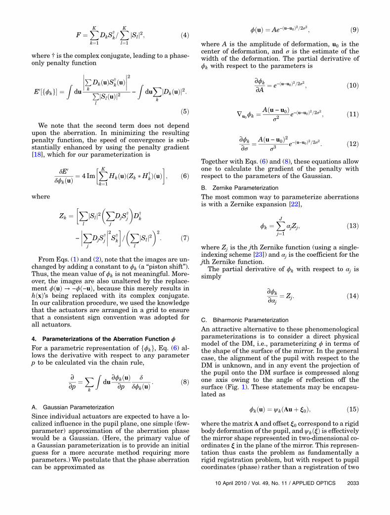
A. Gaussian Parameterization

Since individual actuators are expected to have a lo-calized influence in the pupil plane, one simple (few-parameter) approximation of the aberration phasewould be a Gaussian. (Here, the primary value ofa Gaussian parameterization is to provide an initialguess for a more accurate method requiring moreparameters.) We postulate that the phase aberrationcan be approximated as

ϕðuÞ ¼ Ae−ðu−u0Þ2=2σ2 ; ð9Þ

where A is the amplitude of deformation, u0 is thecenter of deformation, and σ is the estimate of thewidth of the deformation. The partial derivative ofϕk with respect to the parameters is

∂ϕk

∂A¼ e−ðu−u0Þ2=2σ2 ; ð10Þ

∇u0ϕk ¼ Aðu − u0Þσ2 e−ðu−u0Þ2=2σ2 ; ð11Þ

∂ϕk

∂σ ¼ Aðu − u0Þ2σ3 e−ðu−u0Þ2=2σ2 : ð12Þ

Together with Eqs. (6) and (8), these equations allowone to calculate the gradient of the penalty withrespect to the parameters of the Gaussian.

B. Zernike Parameterization

The most common way to parameterize aberrationsis with a Zernike expansion [22],

ϕk ¼XJj¼1

αjZj; ð13Þ

where Zj is the jth Zernike function (using a single-indexing scheme [23]) and αj is the coefficient for thejth Zernike function.

The partial derivative of ϕk with respect to αj issimply

∂ϕk

∂αj¼ Zj: ð14Þ

C. Biharmonic Parameterization

An attractive alternative to these phenomenologicalparameterizations is to consider a direct physicalmodel of the DM, i.e., parameterizing ϕ in terms ofthe shape of the surface of the mirror. In the generalcase, the alignment of the pupil with respect to theDM is unknown, and in any event the projection ofthe pupil onto the DM surface is compressed alongone axis owing to the angle of reflection off thesurface (Fig. 1). These statements may be encapsu-lated as

ϕkðuÞ ¼ ψkðAuþ ξ0Þ; ð15Þ

where thematrixA and offset ξ0 correspond to a rigidbody deformation of the pupil, and ψkðξÞ is effectivelythe mirror shape represented in two-dimensional co-ordinates ξ in the plane of the mirror. This represen-tation thus casts the problem as fundamentally arigid registration problem, but with respect to pupilcoordinates (phase) rather than a registration of two


observed images. A needs to allow rotation andscaling but not shearing (A ¼ RSRT , where R is arotation matrix and S is diagonal), and thus A is ageneric 2 × 2 symmetric matrix

A ¼�a1 a2

a2 a3

�: ð16Þ

After fitting, the rotation angle and scaling diagonalsmay be extracted from a singular value decomposi-tion of A; in particular, the absolute value of the ratioof the diagonals of S should be equal to the cosine ofthe angle of reflection off the mirror surface.The form of ψ depends on the DM. For the Mirao

52-d, the linearity with respect to perturbation ofindividual actuators (see Fig. 5 below) suggests amodel

ψkðξÞ ¼Xi

ðmivki þ ζiÞbiðξÞ; ð17Þ

where vki is the control voltage applied to the ith ac-tuator in the kth diversity image, mi and ζi are theslope and offset for this actuator, respectively, andbiðξÞ describes the shape of the surface induced byapplying unit voltage to the ith actuator; bi encapsu-lates the physics of the device, and in this case thenecessary details (equation of motion and boundaryconditions) are not publicly disclosed by the manu-facturer. However, because this mirror is constructedfrom an elastic membrane, we postulate that themembrane energy is a function of the curvature, i.e.,

Emembrane½b� ∝Z

dξð∇2bÞ2; ð18Þ

where ∇2 is the Laplacian with respect to coordi-nates ξ. Hence b satisfies the fourth-order biharmo-nic equation,

ð∇2Þ2b ¼ 0: ð19Þ

This equation of motion needs to be supplemented bythe boundary conditions, for which we will assumethat the membrane is clamped at some radius Rand that this clamp sets both the membrane heightand slope to zero on the boundary (b ¼ 0 and r̂ ·∇b ¼0 on the boundary, where r̂ is the unit radial vector).Consequently, application of a unit force at point cwill induce a (normalized) displacement given bythe Green’s function [24],

bð~ξj~cÞ ¼ 1

R2 j~ξ − ~cj2 log�R2j~ξ − ~cj2jR2 − ~c†~ξj2

�

þ 1

R4 ðR2 − j~ξj2ÞðR2 − j~cj2Þ; ð20Þ

where ~ξ ¼ ξx þ iξy is the complex number formedfrom the x and y coordinates of ξ and similarly for~c. For each actuator, the corresponding ci is specified

from the known grid arrangement of the actuators[Fig. 2(a)].

The advantage of this approach is in the compara-tively small number of parameters required: ratherthan needing the first five orders of Zernike functions(20 Zernike coefficients for each actuator, a total of1040 parameters), here each actuator is representedby only two parameters, mi and ζi. Indeed, in a first-pass optimization onemay take ζi ¼ 0 and use a com-mon value mi ¼ m for all actuators (assuming thateach electromagnet produces similar force), and thusall 52 actuators contribute just a single parameter,m. One also must fit R and the rigid-deformationparameters A and ξ0, and for calibration with a sin-gle bead we also modify Eq. (15) to allow a defocus,

ϕkðuÞ ¼ ψkðAuþ ξ0Þ þ αð2u2 − 1Þ; ð21Þto include the possibility that the bead is slightlyabove or below the focal plane (which may not bereadily detectable in the mirror flat condition but cannevertheless have a substantial effect on the aber-rated images). Consequently, this approach requiresa total of either 8 parameters (A, ξ0, α, andm) or 110parameters (A, ξ0, α, and susceptibility and offset,miand ζi, respectively, for each actuator).

Optimization of these parameters greatly benefitsfrom an analytic calculation of the gradients; for rea-sons of space we do not present explicit formulas, buttheir derivation from Eqs. (21) and (20) is entirelystraightforward (if slightly tedious). The initial guessfor the eight-parameter model is supplied by the userwith the help of a custom GUI program, to ensurethat the pupil registration parameters do not becometrapped in a local minimum far from the optimumsolution.

5. Experiments

We imaged a 0:2 μm (diffraction-limited) fluorescentbead embedded at the surface of a flat slab of poly-dimethylsiloxane (PDMS, Dow Corning, DC 184-Aand DC 184-B with a weight ratio of 10∶1). Eachactuator was manipulated by applying voltagesranging from −0:1 to 0:1V with 0:01V steps (allthe other actuators were maintained at 0V), and animage was collected at each step. Thus, we obtained21 images for each of the 52 actuators, for a totalof 1092 images. In Fig. 3 we show the images ob-tained by moving one of the actuators [actuator 22,see Fig. 2(a)] from −0:09 to 0:1V (data from all actua-tors is supplied as Media 1).

6. Results

A. Calibration of DM Using Zernike Parameterization

Each actuator was calibrated separately. The image-basedwavefront reconstruction described inSection 3was applied on the 21 images—obtained from apply-ing different voltages to a single actuator—to calcu-late the unknown underlying aberration function ϕ.


1.MOV

http://ao.osa.org/viewmedia.cfm?URI=ao-49-11-2030-1

In the optimization, the initial estimate of ϕ wascreated by fitting a Gaussianmodel of the aberration,which (having far fewer parameters) allowed rapidand relatively exhaustive search. In Fig. 4 we showthat the images obtained by using Gaussian parame-terization of ϕ yielded moderate agreement betweenexperimental and calculated images. We expandedthe ϕ obtained from the Gaussian parameterizationin terms of the first 5 orders of Zernike functions (20parameters in total per actuator) and used the ob-tained Zernike coefficients as the initial guess forthe Zernike-based optimization. We found that thecalculated estimate of ϕ did not improve substan-tially when a larger number of Zernike functionswere used (see Fig. 12 below).In Fig. 5(a) we show the optimized values for

the Zernike coefficients. Each of the Zernike para-meters varies approximately linearly with voltage;the slope of the relationship is plotted as a phase plotin Fig. 5(b). The single-hump peak depicts the move-ment of an actuator at the location of the peak. InFig. 6 we demonstrate the accuracy of the calibrationof one actuator [number 22, Fig. 2(a)] by showing the

measured and calculated images for images obtainedwhen different voltages are applied to this actuator.

Each actuator was calibrated individually with anidentical voltage series comprising 21 images. Oneobserves that the resulting aberrations define a gridstructure reminiscent, as onemight expect, of the un-derlying grid of actuators (Fig. 7). To visualize thealignment between Figs. 2(a) and 7 one needs toreflect the DM actuator grid across the vertical. InMedia 2 we show the measured and calculatedimages obtained for all the actuators.

In Fig. 5(a) we can see that the Zernike coefficientshave a nonzero component at zero applied voltage.This yields an estimate of the baseline aberrationsof the system, which include any imperfections inthe system optics (which tend to be small) and devia-tions in the mirror shape from nominally flat (whichcan be more substantial). In Fig. 8(a) we show thatthe zero offsets measured for each of the actuatorshave similar values even though they were measuredindependently. By calculating the means of the off-sets for each of the 20 Zernike coefficients, we esti-mated the shape of the mirror when all actuatorsare set to zero voltage [Fig. 8(b)]. The flatness of themirror can be improved by supplying an array of off-set voltages v0, with

v0 ¼ −MþZ0; ð22Þ

where Z0 is the vector of Zernike coefficients inthe nominally flat condition, M is the matrix formedfrom the slope of the Zernike coefficients for each ac-tuator [Fig. 5(a)], and + denotes the Moore–Penrosepseudoinverse.

B. Calibration of DM Using a Physical Membrane-BasedModel of DM

We performed the 8- and 110-parameter biharmonicparameterizations of the aberrations caused by indi-vidual actuators. The eight-parameter model wasobtained by using all 21 × 52 images to fit the para-meters A, ξ0, α, and a single value of m for all actua-tors, while setting ζ ¼ 0. The resulting phases foreach of the actuators are shown in Fig. 9.

To obtain the actuator phases for the 110-parameter model, A, ξ0 and α were held constantwhile m and ζ were fitted separately for each actua-tor. In Fig. 10 we show the value of mi obtained foreach of the actuators. The mi values appear to be de-pendent on the location of the corresponding actuator—suggesting an underlying asymmetry in the DM.

In Fig. 11 we show the experimental and calcu-lated images (using biharmonic parameterization)obtained when voltage is applied to actuator 22. Thequality of the agreement is lower than observed forthe Zernike fit (Fig. 6). Therefore, henceforth weadopted the Zernike parameterization.

To quantitatively compare the different parame-terizations implemented in this paper, we calculatedthe fitting error [given by Eq. (3)] for each of the cases(Fig. 12). Gaussian and biharmonic parameteriza-

Fig. 3. Images of a 0:2 μm bead obtained after applying from−0:09 to 0:1V to actuator 22 [see Fig. 2(a) for the location of theactuator]. Each image is 64 × 64 pixels, with 1pixel ¼ 0:29 μm×0:29 μm. (All consequent bead images have the same dimensions).Media 1 shows images obtained from moving each of the 52actuators.

Fig. 4. Measured (top) and calculated (bottom) images of a beadwhen different voltages are applied to actuator 22. The calculatedimages were obtained from the calculated estimate of ϕ usingGaussian parameterization.


2.MOV

1.MOV



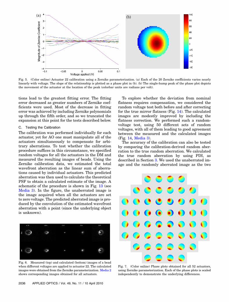
tions lead to the greatest fitting error. The fittingerror decreased as greater numbers of Zernike coef-ficients were used. Most of the decrease in fittingerror was achieved by including Zernike polynomialsup through the fifth order, and so we truncated theexpansion at this point for the tests described below.

C. Testing the Calibration

The calibration was performed individually for eachactuator, yet for AO one must manipulate all of theactuators simultaneously to compensate for arbi-trary aberrations. To test whether the calibrationprocedure suffices in this circumstance, we specifiedrandom voltages for all the actuators in the DM andmeasured the resulting images of beads. Using theZernike calibration data, we estimated the totalwavefront aberration as the linear sum of aberra-tions caused by individual actuators. This predictedaberration was then used to calculate the theoreticalPSF to obtain a calculated estimate of the image. Aschematic of the procedure is shown in Fig. 13 (seeMedia 3). In the figure, the unaberrated image isthe image acquired when all the actuators are setto zero voltage. The predicted aberrated image is pro-duced by the convolution of the estimated wavefrontaberration with a point (since the underlying objectis unknown).

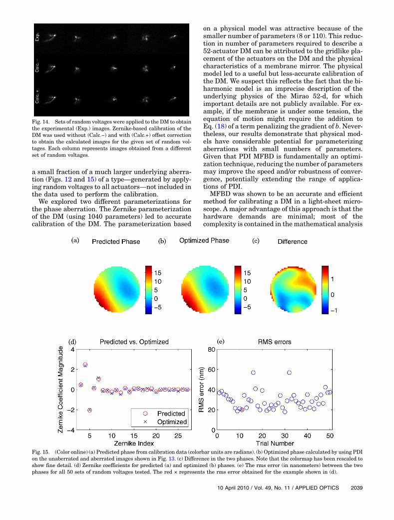
To explore whether the deviation from nominalflatness requires compensation, we considered therandom voltage test both before and after correctingfor the true mirror flatness (Fig. 14). The calculatedimages are modestly improved by including theflatness correction. We performed such a random-voltage test, using 50 different sets of randomvoltages, with all of them leading to good agreementbetween the measured and the calculated images(Fig. 14, Media 3).

The accuracy of the calibration can also be testedby comparing the calibration-derived random aber-ration to the true random aberration. We calculatedthe true random aberration by using PDI, asdescribed in Section 3. We used the unaberrated im-age and the randomly aberrated image as the two

Fig. 5. (Color online) Actuator 22 calibration using a Zernike parameterization. (a) Each of the 20 Zernike coefficients varies nearlylinearly with voltage. The slope of the relationship is plotted as a phase plot in (b). (b) The single-hump peak of the phase plot depictsthe movement of the actuator at the location of the peak (colorbar units are radians per volt).

Fig. 6. Measured (top) and calculated (bottom) images of a beadwhen different voltages are applied to actuator 22. The calculatedimages were obtained from the Zernike parameterization. Media 2shows corresponding images obtained for all actuators.

Fig. 7. (Color online) Phase plots obtained for all 52 actuators,using Zernike parameterization. Each of the phase plots is scaledindependently to demonstrate the underlying differences.


4.MOV




input images and optimized the phase. As an ini-tial estimate we used the calibration-derived phase,which consisted of up to fifth-order Zernike coeffi-cients. To explore a possible role for the higher-ordercoefficients in representing the error, we extendedthe phase to consist of up to sixth-order Zernike coef-ficient, setting the sixth-order Zernike coefficientsinitially to zero. The Zernike coefficients were opti-mized to produce the optimum aberrated phase.Figure 15 shows the calibration-derived phase (pre-dicted phase), the PDI-derived phase (optimizedphase) and the difference in the two phases for theimages shown in Fig. 13. Figure 15(d) shows thatthe calibration-derived estimates for the Zernikecoefficients are very close to the optimized values.We performed the same calculation on each of the

50 sets of the random voltages tested (Media 3)and plotted the rms error in Fig. 15(e). The rms erroraveraged across realizations was ∼30nm, which isbelow the threshold for making a significant impacton image quality. Thus we conclude that the cali-brated DM data yields an accurate model of themirror.

7. Discussion

By using only an image-based analysis we haveshown that MFBD can be used to accurately cali-brate a DM. The decision whether to use MFBD orother methods depends on several factors. (i) Equip-ment: MFBD-based calibration does not require spe-cialized optical equipment such as SHWFS andinterferometers. The MFBD method even avoidsthe need for a beam splitter [19]. (ii) Speed: the speedof wavefront sensing in SHWFS and interfer-ometry—by virtue of being specialized devices tomeasure wavefronts—is nearly instantaneous. In

Fig. 8. (Color online) DM flat. (a) Magnitude of Zernike coeffi-cients for each of the actuators at zero applied voltage obtainedfrom optimization of each actuator independently; note the consis-tency of the fitting result. The first two Zernike coefficients contri-bute to overall tip and tilt of the PSF and are not shown in thisfigure. (b) Phase present at zero applied voltage (colorbar unitsare radians).

Fig. 9. (Color online) Phase plot obtained for all 52 actuators,using the 8-parameter biharmonic parameterization. Each ofthe phase plots is scaled independently to demonstrate the under-lying differences.

Fig. 10. (Color online) Values ofmi obtained for each of the actua-tors after a 110 parameter biharmonic parameterization of ϕ(colorbar units are radians per volt).

Fig. 11. Measured (top) and calculated (middle, bottom) imagesof a bead when different voltages are applied to actuator 22. Thecalculated images were obtained by using a biharmonic parame-terization with 8 (middle) and 110 (bottom) parameters. Media4 shows corresponding images obtained for all actuators.


4.MOV

3.MOV

3.MOV




MFBD-based calibration, the wavefront calculationis a computationally intensive process. The calibra-tion of a single actuator, using 21 images (seeSection 6) took ∼3 min (this includes a preliminaryGUI-based Gaussian estimate, followed by aZernike-based optimization of the aberration func-tion ϕ) on a 32Gbyte RAM, single-core processor.Thus the calibration of the 52 actuator DM took∼2:5h. Fortunately, such a CPU-intensive calcula-

tion needs to be performed only once, during theconstruction of the microscope. (iii) Accuracy: theMFBD-based calibration is ultimately limited by thenoise in the images. We have shown that the methodproduces an error of ∼30nm, which is well below thethreshold where the error has a significant impact onthe image quality. We note that this accuracy com-pares well with previous studies [19], in that this re-presents the open-loop calibration error, and that it is

Fig. 12. (Color online) Comparison of fitting errors: (a) fitting error between experimental and calculated images using different ϕ para-meterizations, for actuator 22. The different parameterizations are Gaussian (G), from second- to eighth-order Zernike parameters, bi-harmonic parameterization using 8 parameters (B8), and biharmonic parameterization using 110 parameters (B110). (b) Total fitting errorbetween the experimental and calculated images for all actuators.

Fig. 13. (Color online) A random set of voltages are applied to the DM to produce the acquired image. The Zernike-parameterization-based calibration of the DM is used to calculate the predicted phase produced by the set of random voltages (colorbar units are radians).The predicted phase is then used to create the predicted image. The agreement between the acquired and predicted images demonstratesthe accuracy of the calibration of the DM. Media 3 shows images obtained from using the 50 sets of random voltages.


4.MOV


a small fraction of a much larger underlying aberra-tion (Figs. 12 and 15) of a type—generated by apply-ing random voltages to all actuators—not included inthe data used to perform the calibration.We explored two different parameterizations for

the phase aberration. The Zernike parameterizationof the DM (using 1040 parameters) led to accuratecalibration of the DM. The parameterization based

on a physical model was attractive because of thesmaller number of parameters (8 or 110). This reduc-tion in number of parameters required to describe a52-actuator DM can be attributed to the gridlike pla-cement of the actuators on the DM and the physicalcharacteristics of a membrane mirror. The physicalmodel led to a useful but less-accurate calibration ofthe DM. We suspect this reflects the fact that the bi-harmonic model is an imprecise description of theunderlying physics of the Mirao 52-d, for whichimportant details are not publicly available. For ex-ample, if the membrane is under some tension, theequation of motion might require the addition toEq. (18) of a term penalizing the gradient of b. Never-theless, our results demonstrate that physical mod-els have considerable potential for parameterizingaberrations with small numbers of parameters.Given that PDI MFBD is fundamentally an optimi-zation technique, reducing the number of parametersmay improve the speed and/or robustness of conver-gence, potentially extending the range of applica-tions of PDI.

MFBD was shown to be an accurate and efficientmethod for calibrating a DM in a light-sheet micro-scope. A major advantage of this approach is that thehardware demands are minimal; most of thecomplexity is contained in themathematical analysis

Fig. 14. Sets of random voltages were applied to the DM to obtainthe experimental (Exp.) images. Zernike-based calibration of theDM was used without (Calc:−) and with (Calc.+) offset correctionto obtain the calculated images for the given set of random vol-tages. Each column represents images obtained from a differentset of random voltages.

Fig. 15. (Color online) (a) Predicted phase from calibration data (colorbar units are radians). (b) Optimized phase calculated by using PDIon the unaberrated and aberrated images shown in Fig. 13. (c) Difference in the two phases. Note that the colormap has been rescaled toshow fine detail. (d) Zernike coefficients for predicted (a) and optimized (b) phases. (e) The rms error (in nanometers) between the twophases for all 50 sets of random voltages tested. The red × represents the rms error obtained for the example shown in (d).


and therefore encapsulated in software. We havemade our software freely available at http://holylab.wustl.edu. These developments should contributeto more widespread application of AO in microscopy.

The authors thank Zhongsheng Guo for com-putational help. The research was supported bythe McKnight Technological Innovations in Neu-roscience Award and the National Institutes ofHealth (NINDS/NIAAA R01NS068409, T. E. Holy).

References1. J. B. Pawley, Handbook of Biological Confocal Microscopy, 3rd

ed. (Springer, 2006).2. J. J. J. Dirckx, L. C. Kuypers, andW. F. Decraemer, “Refractive

index of tissuemeasured with confocal microscopy,” J. Biomed.Opt. 10, 044014 (2005).

3. M. J. Booth, “Adaptive optics in microscopy,” Philos. Transact.R. Soc. A. 365, 2829–2843 (2007).

4. D. Turaga and T. E. Holy, “Miniaturization and defocus correc-tion for objective-coupled planar illumination microscopy,”Opt. Lett. 33, 2302–2304 (2008).

5. T. F. Holekamp, D. Turaga, and T. E. Holy, “Fast three-dimen-sional fluorescence imaging of activity in neural populationsby objective-coupled planar illumination microscopy,” Neuron57, 661–672 (2008).

6. E. Fuchs, J. S. Jaffe, R. A. Long, and F. Azam, “Thin laser lightsheet microscope for microbial oceanography,” Opt. Express10, 145–154 (2002).

7. J. Huisken, J. Swoger, F. Del Bene, J. Wittbrodth, andE. H. K. Stelzer, “Optical sectioning deep inside live embryosby selective plane illumination microscopy,” Science 305,1007–1009 (2004).

8. H.-U. Dodt, U. Leischner, A. Schierloh, N. Jährling,C. P. Mauch, K. Deininger, J. M. Deussing, M. Eder,W. Zieglgänsberger, and K. Becker, “Ultramicroscopy: three-dimensional visualization of neuronal networks in the wholemouse brain,” Nat. Methods 4, 331–336 (2007).

9. R.K.Tyson, Introduction toAdaptiveOptics (SPIEPress,2000).

10. J. Porter, H. Queener, J. Lin, K. Thorn, and A. Awwal, Adap-tive Optics for Vision Science (Wiley-Interscience, 2006).

11. L. A. Poyneer, “Scene-based Shack–Hartmann wave-frontsensing: analysis and simulation,” Appl. Opt. 42, 5807–5815(2003).

12. M. Feierabend, M. Ruckel, and W. Denk, “Coherence-gatedwave-front sensing in strongly scattering samples,” Opt. Lett.29, 2255–2257 (2004).

13. B. Hermann, E. J. Fernandez, A. Unterhuber, H. Sattmann,A. F. Fercher, W. Drexler, P. M. Prieto, and P. Artal,“Adaptive-optics ultrahigh-resolution optical coherence to-mography,” Opt. Lett. 29, 2142–2144 (2004).

14. M. J. Booth, M. A. A. Neil, R. Juškaitis, and T. Wilson, “Adap-tive aberration correction in a confocal microscope,” Proc.Natl. Acad. Sci. USA 99, 5788–5792 (2002).

15. D. Debarre, E. J. Botcherby, T. Watanabe, S. Srinivas,M. J. Booth, and T. Wilson, “Image-based adaptive opticsfor two-photon microscopy,” Opt. Lett. 34, 2495–2497 (2009).

16. B. M. Hanser, M. G. L. Gustafsson, D. A. Agard, andJ. W. Sedat, “Phase-retrieved pupil functions in wide-fieldfluorescence microscopy,” J. Microscopy 216, 32–48 (2004).

17. R. A. Gonsalves, “Phase retrieval and diversity in adaptive op-tics,” Opt. Eng. 21, 829–832 (1982).

18. R. G. Paxman, T. J. Schulz, and J. R. Fienup, “Joint estimationof object and aberrations by using phase diversity,” J. Opt. Soc.Am. A 9, 1072–1085 (1992).

19. M. G. Lofdahl, G. B. Scharmer, and W. Wei, “Calibration of adeformable mirror and Strehl ratio measurements by use ofphase diversity,” Appl. Opt. 39, 94–103 (2000).

20. T. J. Schulz, “Multi-frame blind deconvolution of astronomicalimages,” J. Opt. Soc. Am. A 10, 1064–1073 (1993).

21. E. J. Fernandez, L. Vabre, B. Hermann, A. Unterhuber,B. Povazay, and W. Drexler, “Adaptive optics with a magneticdeformable mirror: applications in the human eye,” Opt. Ex-press 14, 8900–8917 (2006).

22. M. Born and E. Wolf, Principles of Optics (Pergamon, , 1986).23. R. J. Noll, “Zernike polynomials and atmospheric turbulence,”

J. Opt. Soc. Am. 66, 207–211 (1976).24. Y. A. Melnikov, “Influence functions of a point force for Kirchh-

off plates with rigid inclusions,” J. Mec. 20, 249–256 (2004).


http://holylab.wustl.edu



Documents

Image-based calibration of a deformable mirror in wide-field