Embed Size (px)
Citation preview
University of Ioannina - Department of Computer Science and Engineering
Christophoros Nikou
Image Analysis
Images taken from:
Computer Vision course by Kristen Grauman, University of Texas at Austin
(http://www.cs.utexas.edu/~grauman/courses/spring2011/index.html).
D. Forsyth and J. Ponce. Computer Vision: A Modern Approach, Prentice Hall, 2003.
R. Gonzalez and R. Woods. Digital Image Processing, Prentice Hall, 2008.
Simon J.D. Prince. Computer vision: models, learning and inference, Cambridge U.P., 2011
Texture
2
C. Nikou – Image Analysis (T-14)
What is Texture?
• No formal definition exists
– Coarseness, regularity, smoothness.
– Whether an effect is textured depends on the
scale it is viewed.
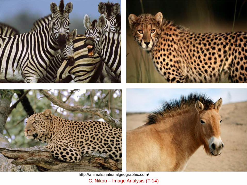
• A leaf occupying an image is an object but the
foliage of a tree is considered texture.
– Large numbers of small objects are texture
(pebbles, grass, brush etc.).
– Surfaces with orderly patterns (spots of
leopards, stripes of zebras, wood etc.).
3
C. Nikou – Image Analysis (T-14)
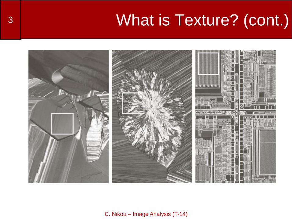
What is Texture? (cont.)
4
C. Nikou – Image Analysis (T-14)
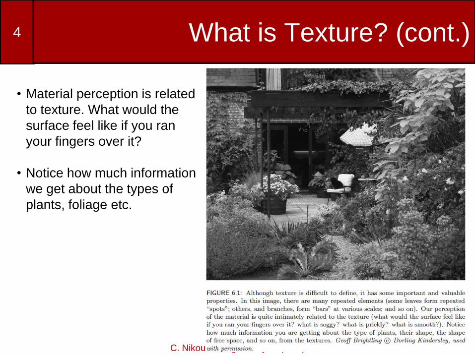
What is Texture? (cont.)
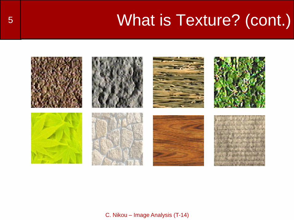
• Material perception is related
to texture. What would the
surface feel like if you ran
your fingers over it?
• Notice how much information
we get about the types of
plants, foliage etc.
5
C. Nikou – Image Analysis (T-14)
What is Texture? (cont.)
6
C. Nikou – Image Analysis (T-14)
What is Texture? (cont.)
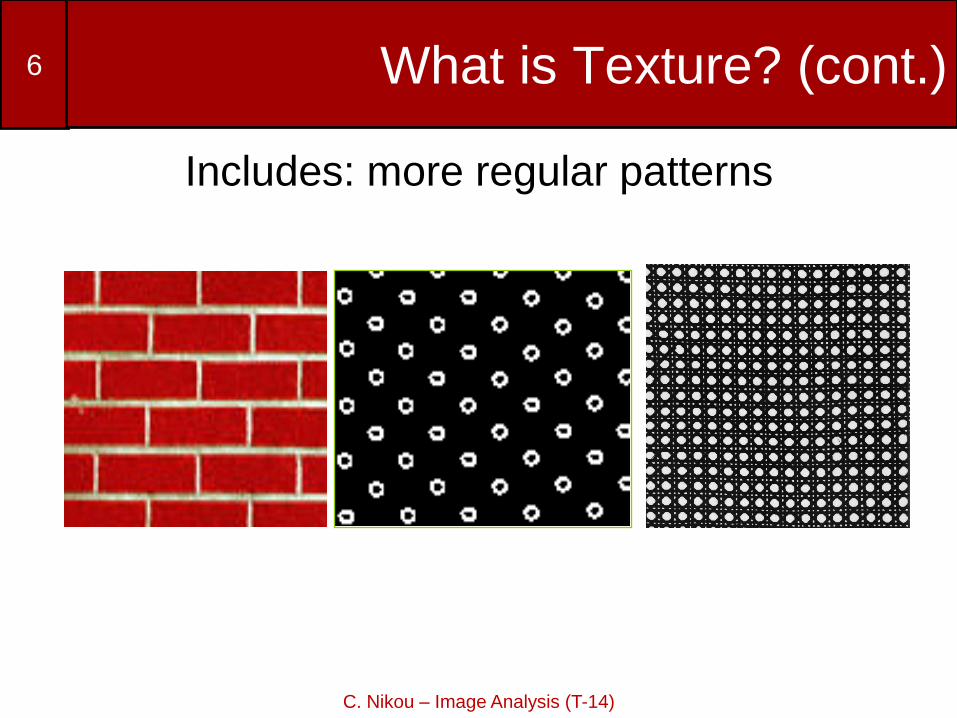
Includes: more regular patterns
7
C. Nikou – Image Analysis (T-14)
What is Texture? (cont.)
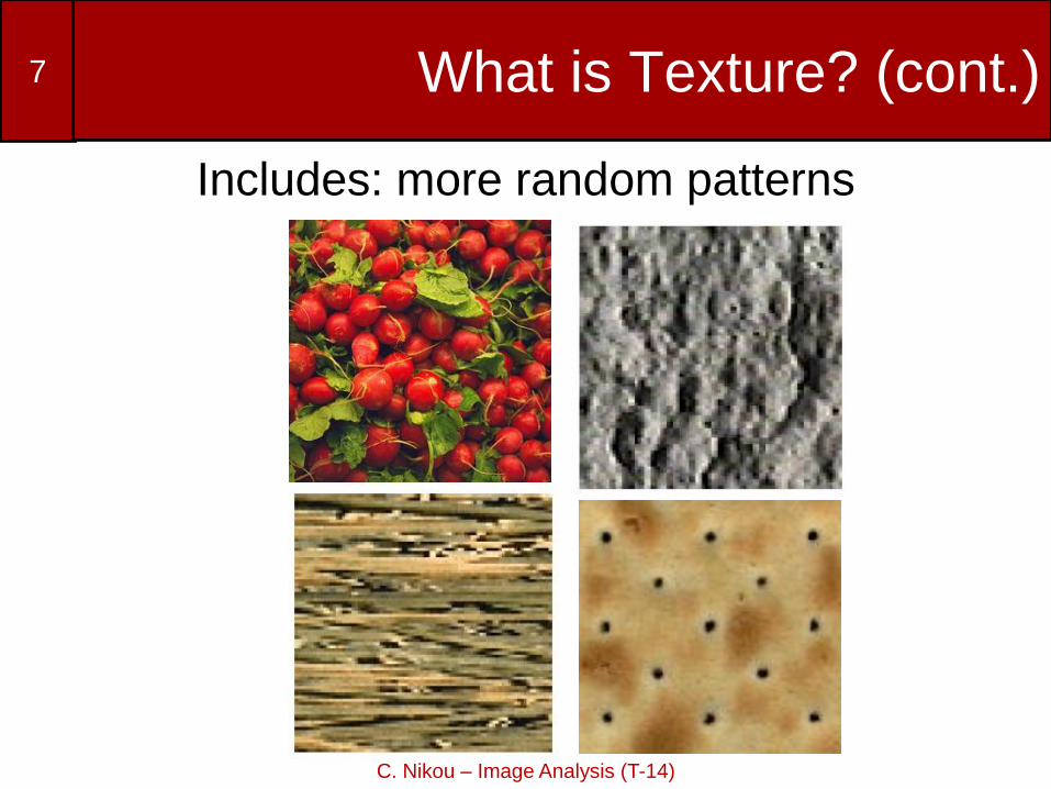
Includes: more random patterns
8
C. Nikou – Image Analysis (T-14)
Texture issues
• Texture analysis (segmentation)
–Key issue: representing texture
• Texture synthesis
– Create big textures for computer graphics
– Fill in holes in images caused by editing
• Shape from texture
–Recover shape orientation from an image.
• We will not talk about it in this course.
9
C. Nikou – Image Analysis (T-14)
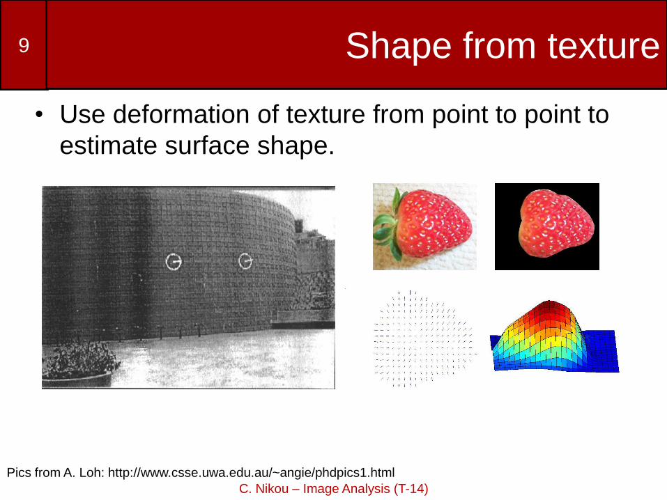
Shape from texture
• Use deformation of texture from point to point to
estimate surface shape.
Pics from A. Loh: http://www.csse.uwa.edu.au/~angie/phdpics1.html
10
C. Nikou – Image Analysis (T-14)
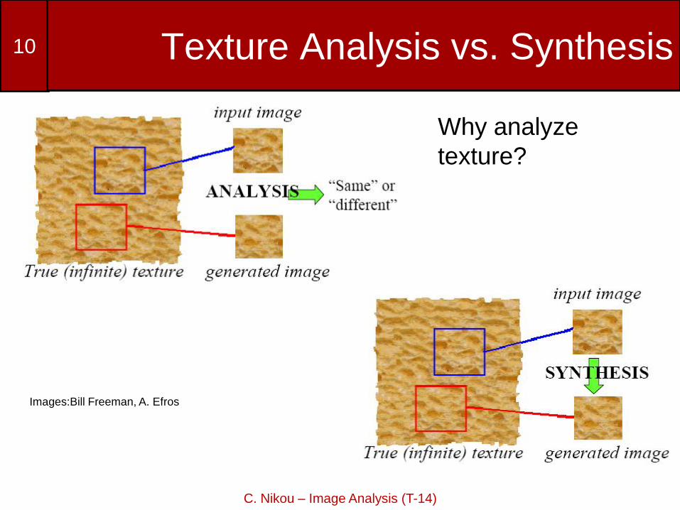
Texture Analysis vs. Synthesis
Images:Bill Freeman, A. Efros
Why analyze
texture?
11
C. Nikou – Image Analysis (T-14)
12
C. Nikou – Image Analysis (T-14)
13
C. Nikou – Image Analysis (T-14)
http://animals.nationalgeographic.com/
14
C. Nikou – Image Analysis (T-14)
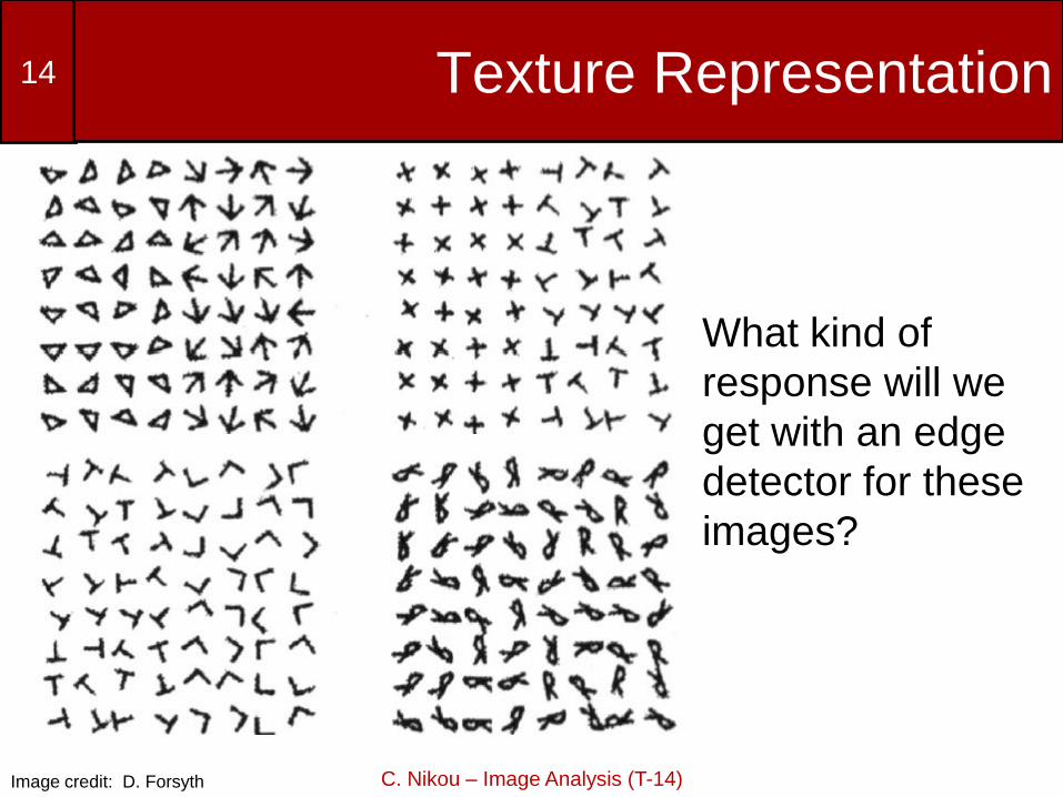
Texture Representation
Image credit: D. Forsyth
What kind of
response will we
get with an edge
detector for these
images?
15
C. Nikou – Image Analysis (T-14)
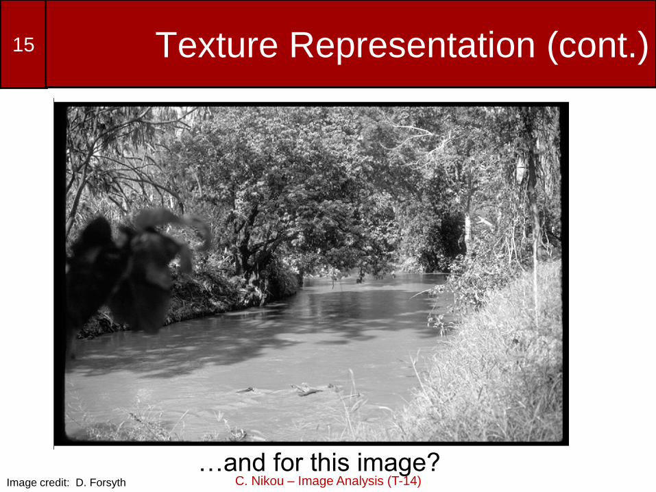
Texture Representation (cont.)
…and for this image?Image credit: D. Forsyth
16
C. Nikou – Image Analysis (T-14)
Why analyze texture?
Importance to perception:
• Often indicative of a material’s properties
• Can be important appearance cue, especially if
shape is similar across objects
Technically:
• Representation-wise, we want a feature one
step above ―building blocks‖ of filters, edges.
17
C. Nikou – Image Analysis (T-14)
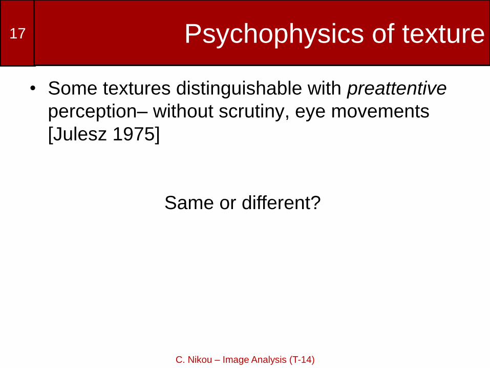
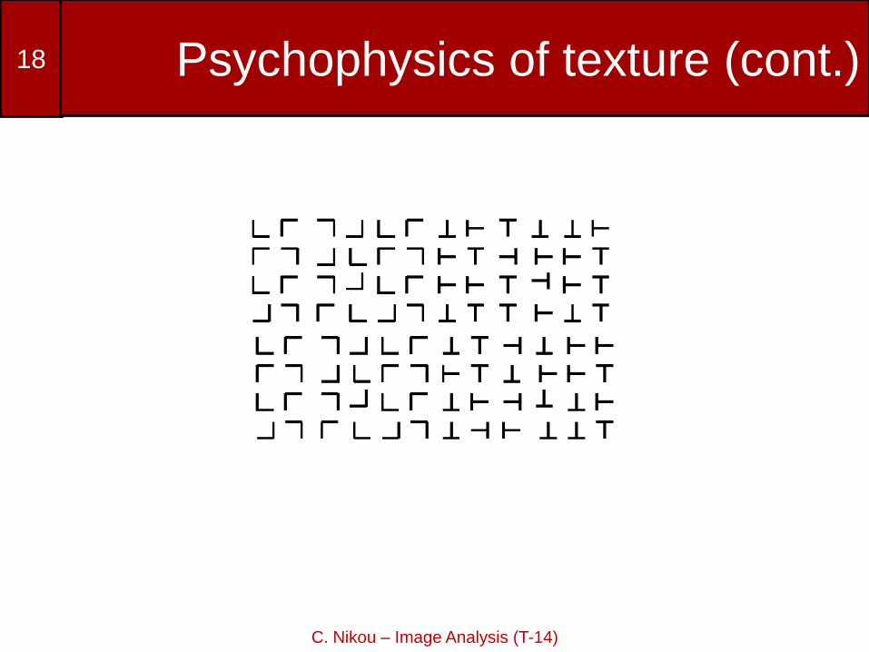
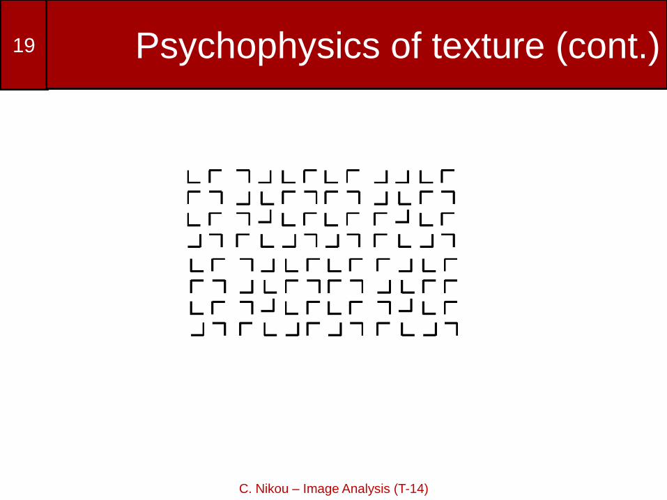
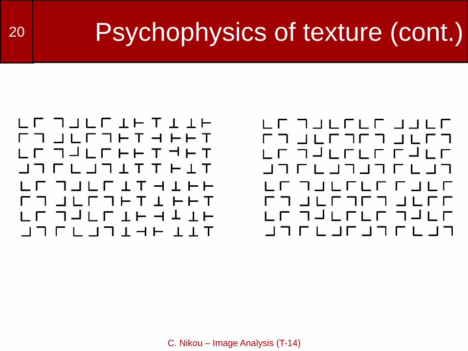
• Some textures distinguishable with preattentive
perception– without scrutiny, eye movements
[Julesz 1975]
Same or different?
Psychophysics of texture
18
C. Nikou – Image Analysis (T-14)
Psychophysics of texture (cont.)
19
C. Nikou – Image Analysis (T-14)
Psychophysics of texture (cont.)
20
C. Nikou – Image Analysis (T-14)
Psychophysics of texture (cont.)
21
C. Nikou – Image Analysis (T-14)
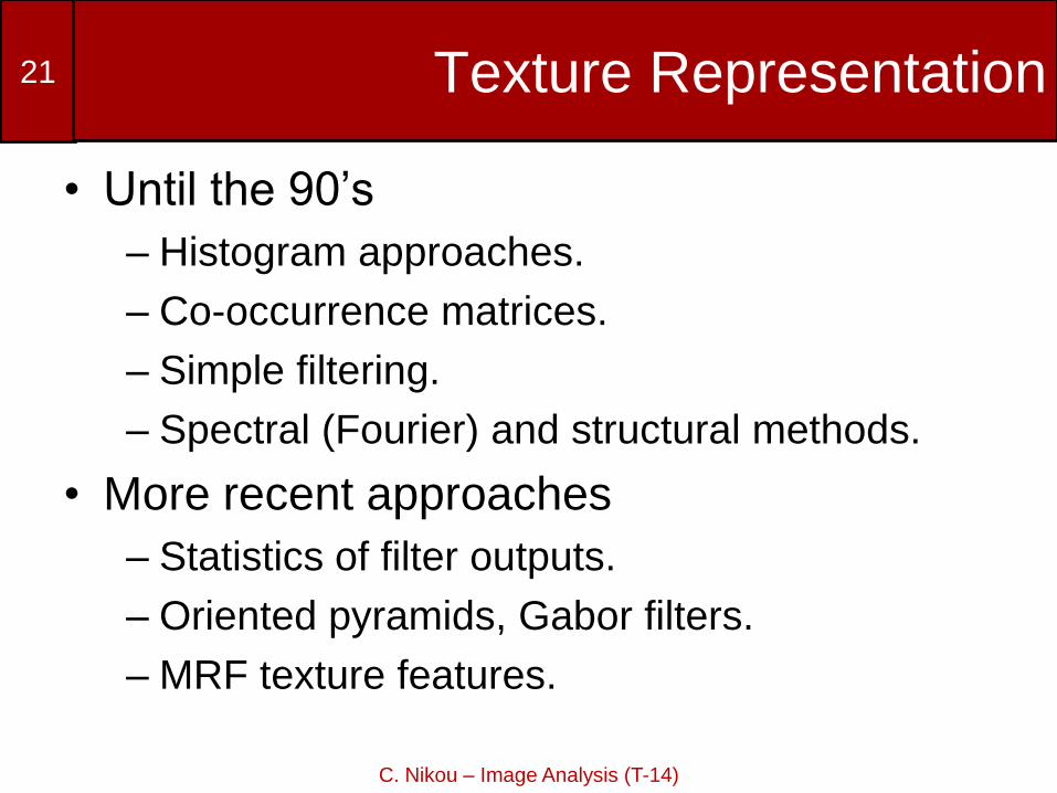
Texture Representation
• Until the 90’s
– Histogram approaches.
– Co-occurrence matrices.
– Simple filtering.
– Spectral (Fourier) and structural methods.
• More recent approaches
– Statistics of filter outputs.
– Oriented pyramids, Gabor filters.
– MRF texture features.
22
C. Nikou – Image Analysis (T-14)
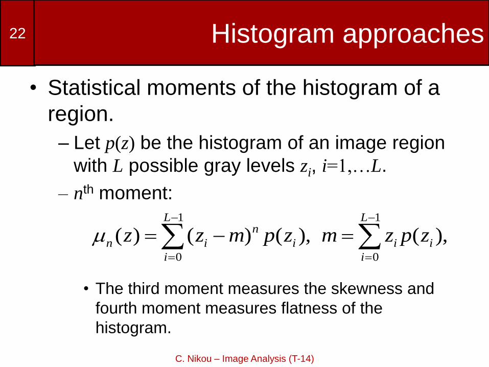
Histogram approaches
• Statistical moments of the histogram of a
region.
– Let p(z) be the histogram of an image region
with L possible gray levels zi, i=1,…L.
– nth moment:
• The third moment measures the skewness and
fourth moment measures flatness of the
histogram.
1 1
0 0
( ) ( ) ( ), ( ),L L
n
n i i i i
i i
z z m p z m z p z
23
C. Nikou – Image Analysis (T-14)
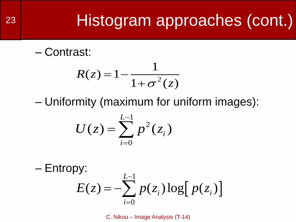
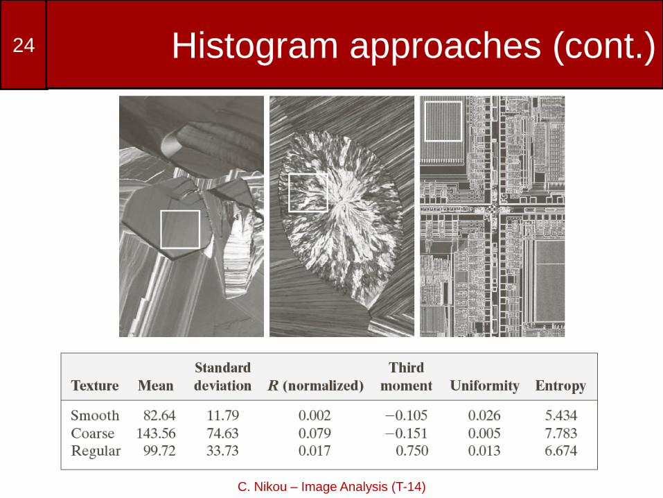
Histogram approaches (cont.)
– Contrast:
– Uniformity (maximum for uniform images):
– Entropy:
12
0
( ) ( )L
i
i
U z p z
1
0
( ) ( ) log ( )L
i i
i
E z p z p z
2
1( ) 1
1 ( )R z
z
24
C. Nikou – Image Analysis (T-14)
Histogram approaches (cont.)
25
C. Nikou – Image Analysis (T-14)
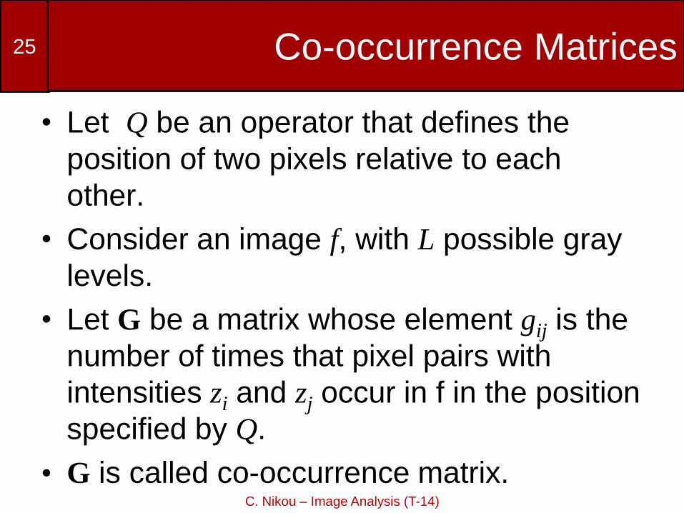
Co-occurrence Matrices
• Let Q be an operator that defines the
position of two pixels relative to each
other.
• Consider an image f, with L possible gray
levels.
• Let G be a matrix whose element gij is the
number of times that pixel pairs with
intensities zi and zj occur in f in the position
specified by Q.
• G is called co-occurrence matrix.
26
C. Nikou – Image Analysis (T-14)
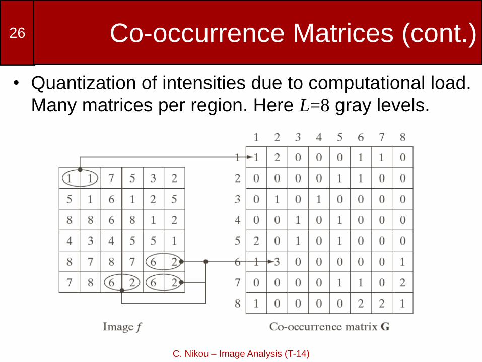
Co-occurrence Matrices (cont.)
• Quantization of intensities due to computational load.
Many matrices per region. Here L=8 gray levels.
27
C. Nikou – Image Analysis (T-14)
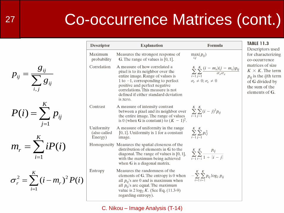
Co-occurrence Matrices (cont.)
,
ij
ij
ij
i j
gp
g
1
( )K
ij
j
P i p
1
( )K
r
i
m iP i
2 2
1
( ) ( )K
r r
i
i m P i
28
C. Nikou – Image Analysis (T-14)
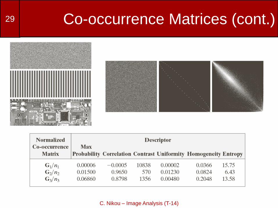
Co-occurrence Matrices (cont.)
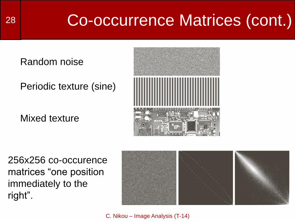
Random noise
Periodic texture (sine)
Mixed texture
256x256 co-occurence
matrices ―one position
immediately to the
right‖.
29
C. Nikou – Image Analysis (T-14)
Co-occurrence Matrices (cont.)
30
C. Nikou – Image Analysis (T-14)
Co-occurrence Matrices (cont.)
• Is there an image portion containing a certain
texture?
• Sequences of co-occurrence matrices are
employed.
• For example, the correlation descriptor for
varying horizontal offset of adjacent pixels
may be calculated.
• In the next experiment, this is performed for
co-occurence matrices computed for
horizontal offsets from 1 to 50 pixels.
31
C. Nikou – Image Analysis (T-14)
Co-occurrence Matrices (cont.)
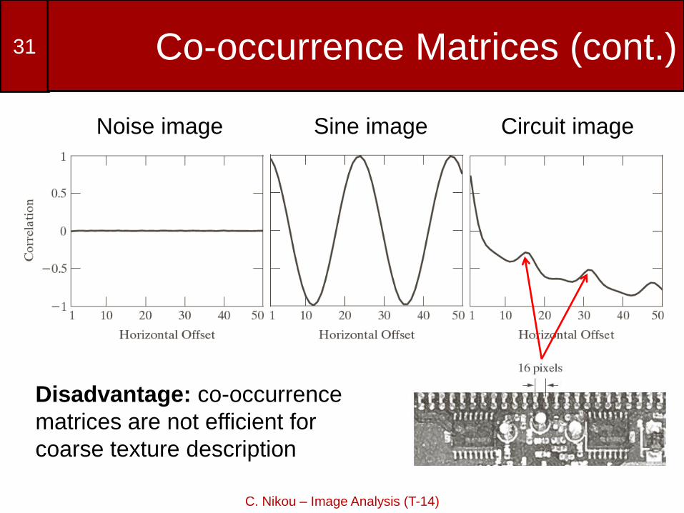
Noise image Sine image Circuit image
Disadvantage: co-occurrence
matrices are not efficient for
coarse texture description
32
C. Nikou – Image Analysis (T-14)
A Spectral Approach
• The Fourier transform (FT) is useful for
description of the directionality of periodic or
almost periodic structures.
– Peaks in the FT give the principal direction of
patterns.
– The location of peaks gives the fundamental
period of patterns.
– The FT is symmetric around the origin and only
half of the frequency plane needs to be
considered.
33
C. Nikou – Image Analysis (T-14)
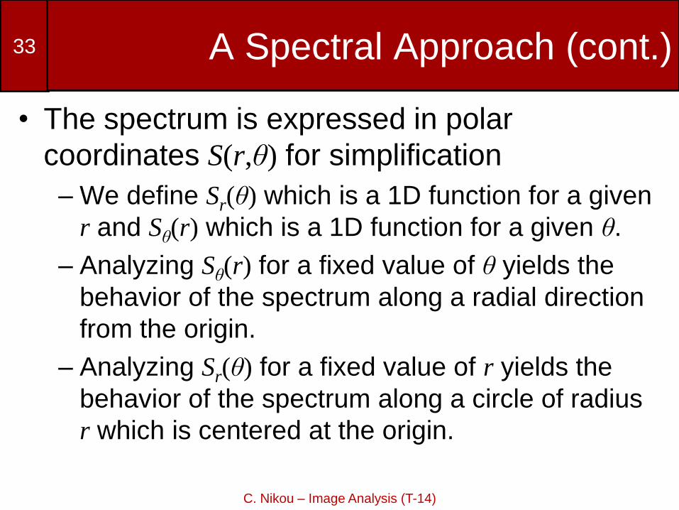
A Spectral Approach (cont.)
• The spectrum is expressed in polar
coordinates S(r,θ) for simplification
– We define Sr(θ) which is a 1D function for a given
r and Sθ(r) which is a 1D function for a given θ.
– Analyzing Sθ(r) for a fixed value of θ yields the
behavior of the spectrum along a radial direction
from the origin.
– Analyzing Sr(θ) for a fixed value of r yields the
behavior of the spectrum along a circle of radius
r which is centered at the origin.
34
C. Nikou – Image Analysis (T-14)
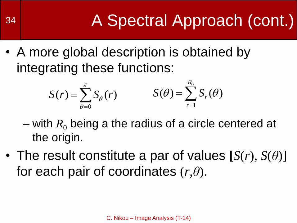
A Spectral Approach (cont.)
• A more global description is obtained by
integrating these functions:
– with R0 being a the radius of a circle centered at
the origin.
• The result constitute a par of values [S(r), S(θ)]
for each pair of coordinates (r,θ).
0
( ) ( )S r S r
0
1
( ) ( )R
r
r
S S
35
C. Nikou – Image Analysis (T-14)
A Spectral Approach (cont.)
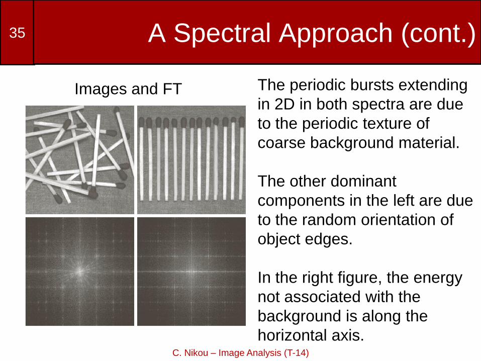
Images and FT The periodic bursts extending
in 2D in both spectra are due
to the periodic texture of
coarse background material.
The other dominant
components in the left are due
to the random orientation of
object edges.
In the right figure, the energy
not associated with the
background is along the
horizontal axis.
36
C. Nikou – Image Analysis (T-14)
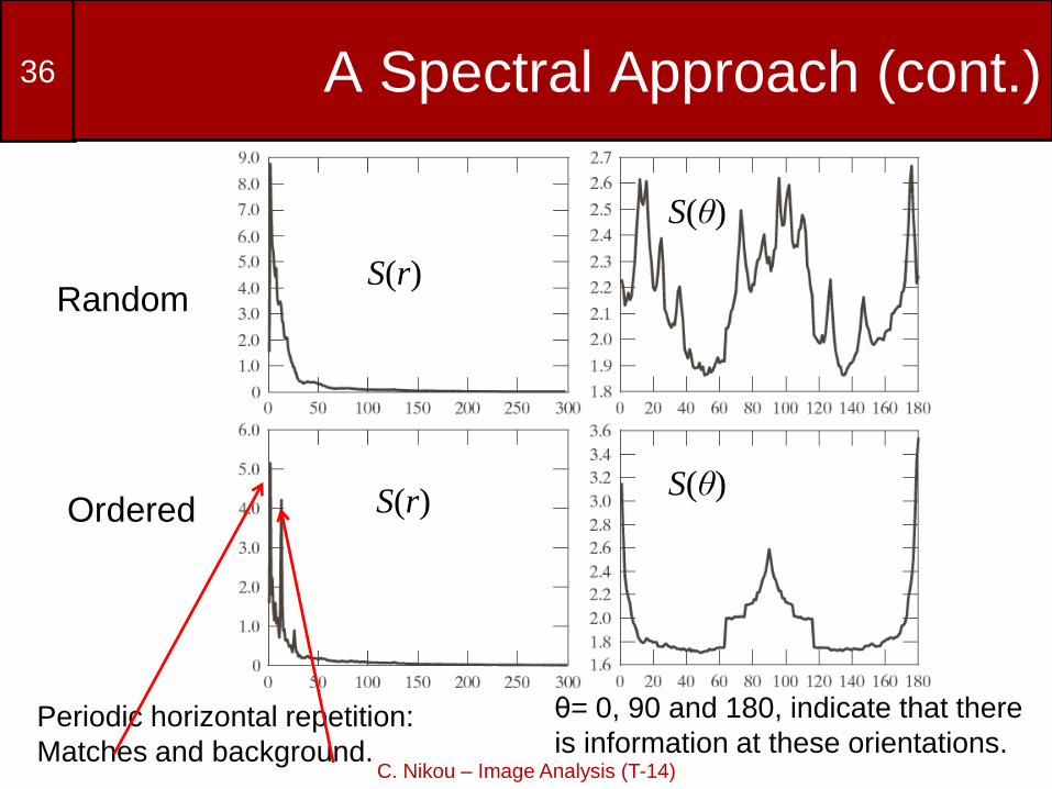
A Spectral Approach (cont.)
Random
Ordered
Periodic horizontal repetition:
Matches and background.
S(r)
S(r)
S(θ)
S(θ)
θ= 0, 90 and 180, indicate that there
is information at these orientations.
37
C. Nikou – Image Analysis (T-14)
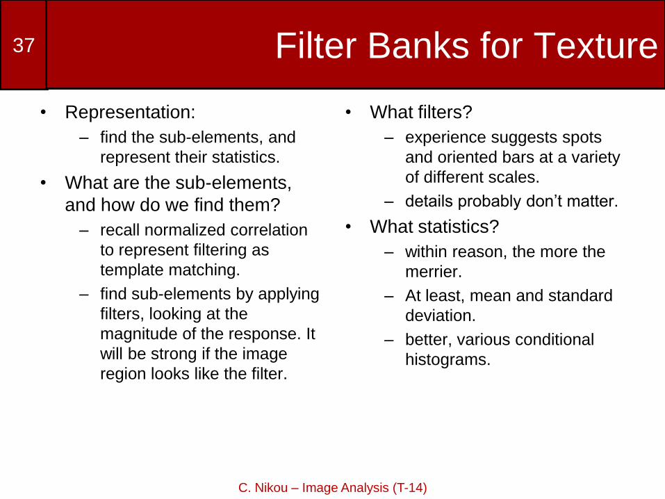
Filter Banks for Texture
• Representation:
– find the sub-elements, and
represent their statistics.
• What are the sub-elements,
and how do we find them?
– recall normalized correlation
to represent filtering as
template matching.
– find sub-elements by applying
filters, looking at the
magnitude of the response. It
will be strong if the image
region looks like the filter.
• What filters?
– experience suggests spots
and oriented bars at a variety
of different scales.
– details probably don’t matter.
• What statistics?
– within reason, the more the
merrier.
– At least, mean and standard
deviation.
– better, various conditional
histograms.
38
C. Nikou – Image Analysis (T-14)
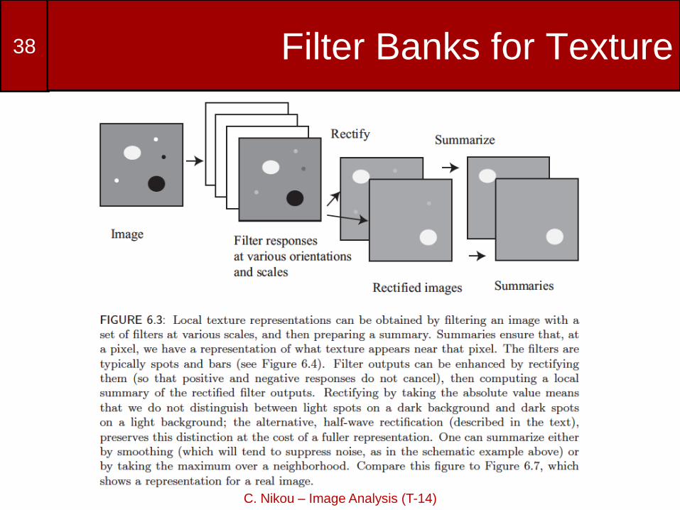
Filter Banks for Texture
39
C. Nikou – Image Analysis (T-14)
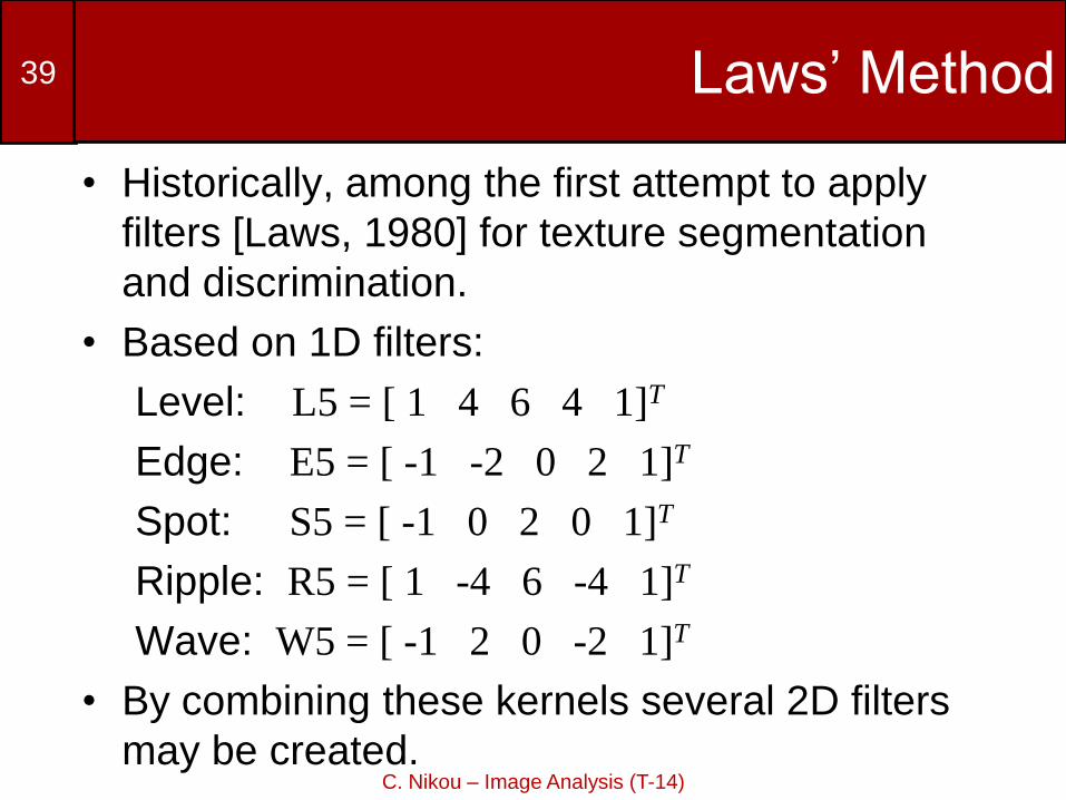
Laws’ Method
• Historically, among the first attempt to apply
filters [Laws, 1980] for texture segmentation
and discrimination.
• Based on 1D filters:
Level: L5 = [ 1 4 6 4 1]T
Edge: E5 = [ -1 -2 0 2 1]T
Spot: S5 = [ -1 0 2 0 1]T
Ripple: R5 = [ 1 -4 6 -4 1]T
Wave: W5 = [ -1 2 0 -2 1]T
• By combining these kernels several 2D filters
may be created.
40
C. Nikou – Image Analysis (T-14)
Laws’ Method (cont.)
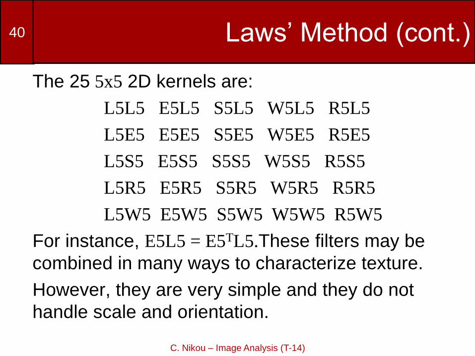
The 25 5x5 2D kernels are:
L5L5 E5L5 S5L5 W5L5 R5L5
L5E5 E5E5 S5E5 W5E5 R5E5
L5S5 E5S5 S5S5 W5S5 R5S5
L5R5 E5R5 S5R5 W5R5 R5R5
L5W5 E5W5 S5W5 W5W5 R5W5
For instance, E5L5 = E5TL5.These filters may be
combined in many ways to characterize texture.
However, they are very simple and they do not
handle scale and orientation.
41
C. Nikou – Image Analysis (T-14)
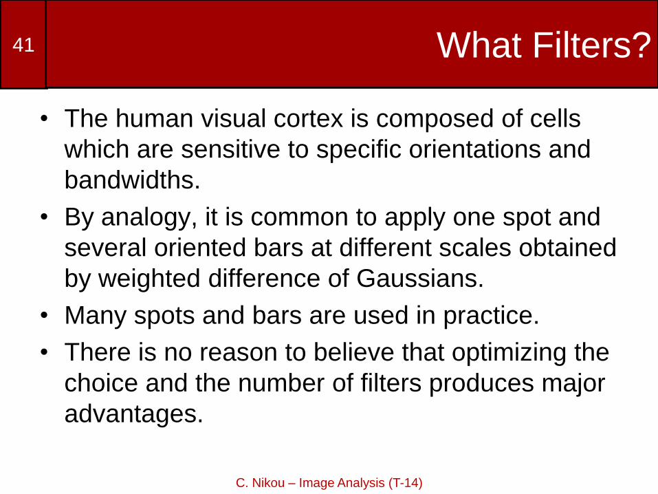
What Filters?
• The human visual cortex is composed of cells
which are sensitive to specific orientations and
bandwidths.
• By analogy, it is common to apply one spot and
several oriented bars at different scales obtained
by weighted difference of Gaussians.
• Many spots and bars are used in practice.
• There is no reason to believe that optimizing the
choice and the number of filters produces major
advantages.
42
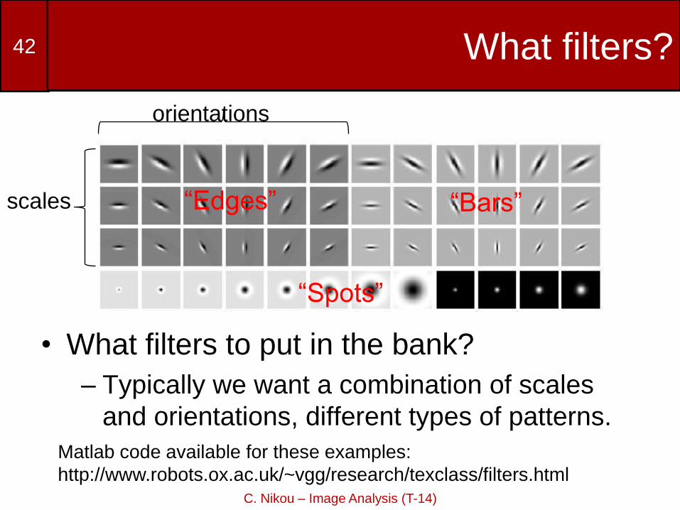
C. Nikou – Image Analysis (T-14)
• What filters to put in the bank?
– Typically we want a combination of scales
and orientations, different types of patterns.
Matlab code available for these examples:
http://www.robots.ox.ac.uk/~vgg/research/texclass/filters.html
scales
orientations
―Edges‖ ―Bars‖
―Spots‖
What filters?
43
C. Nikou – Image Analysis (T-14)
90
09
90
016
55
510
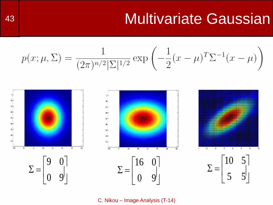
Multivariate Gaussian
44
C. Nikou – Image Analysis (T-14)
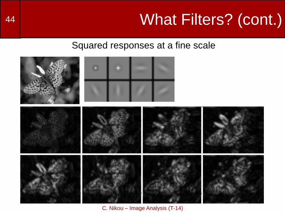
What Filters? (cont.)
Squared responses at a fine scale
45
C. Nikou – Image Analysis (T-14)
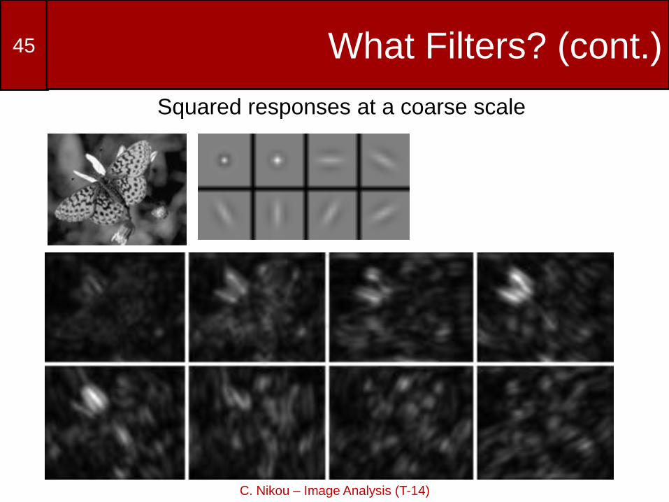
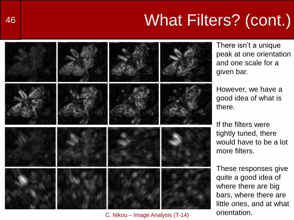
What Filters? (cont.)
Squared responses at a coarse scale
46
C. Nikou – Image Analysis (T-14)
What Filters? (cont.)
There isn’t a unique
peak at one orientation
and one scale for a
given bar.
However, we have a
good idea of what is
there.
If the filters were
tightly tuned, there
would have to be a lot
more filters.
These responses give
quite a good idea of
where there are big
bars, where there are
little ones, and at what
orientation.
47
C. Nikou – Image Analysis (T-14)
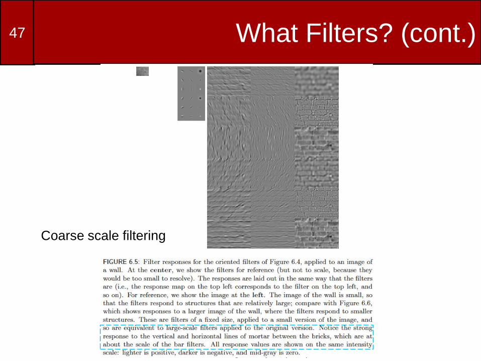
What Filters? (cont.)
Coarse scale filtering
48
C. Nikou – Image Analysis (T-14)
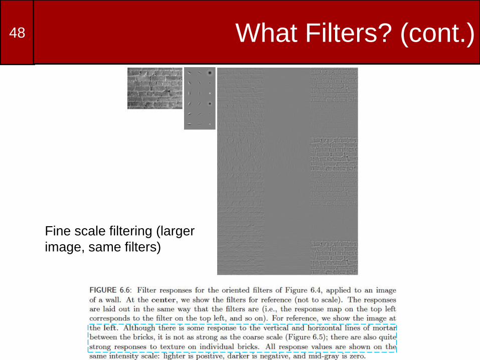
What Filters? (cont.)
Fine scale filtering (larger
image, same filters)
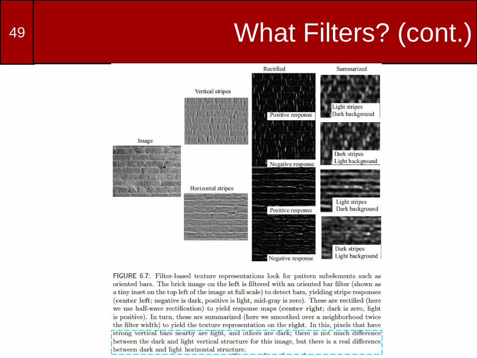
49
C. Nikou – Image Analysis (T-14)
What Filters? (cont.)
50
C. Nikou – Image Analysis (T-14)
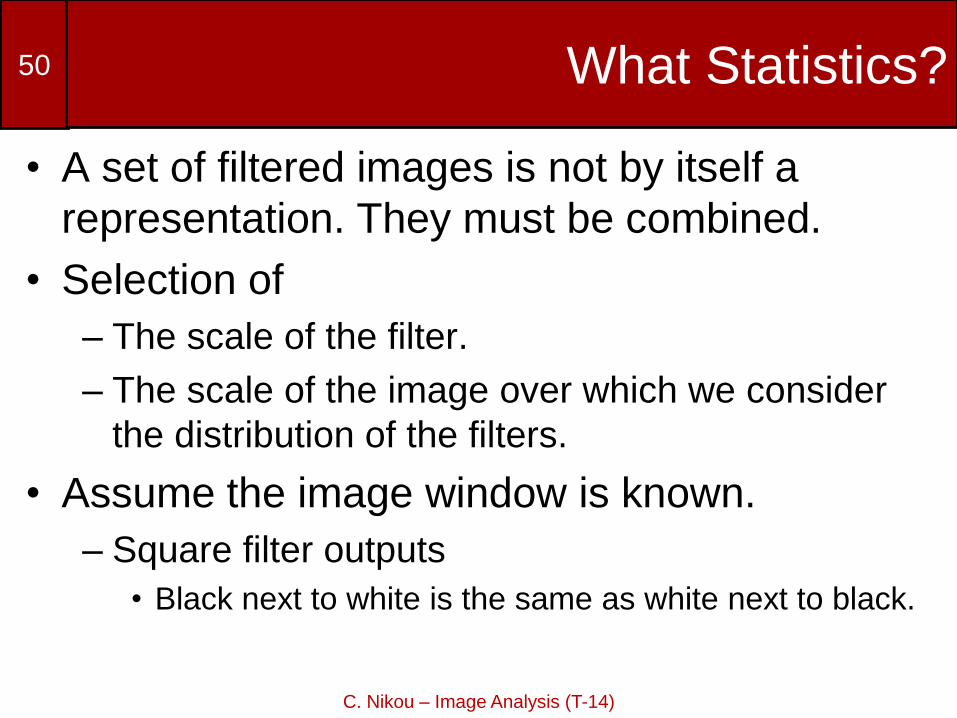
What Statistics?
• A set of filtered images is not by itself a
representation. They must be combined.
• Selection of
– The scale of the filter.
– The scale of the image over which we consider
the distribution of the filters.
• Assume the image window is known.
– Square filter outputs
• Black next to white is the same as white next to black.
51
C. Nikou – Image Analysis (T-14)
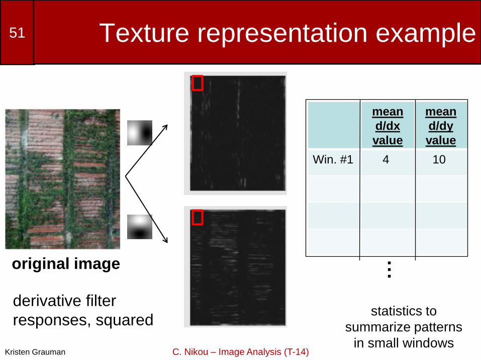
original image
derivative filter
responses, squaredstatistics to
summarize patterns
in small windows
mean
d/dx
value
mean
d/dy
value
Win. #1 4 10
…
Kristen Grauman
Texture representation example

52
C. Nikou – Image Analysis (T-14)
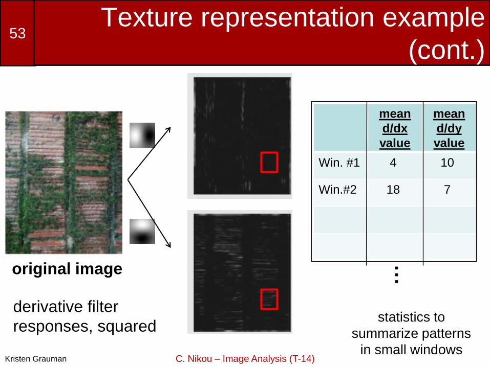
original image
mean
d/dx
value
mean
d/dy
value
Win. #1 4 10
Win.#2 18 7
…
Kristen Grauman
derivative filter
responses, squaredstatistics to
summarize patterns
in small windows
Texture representation example
(cont.)
53
C. Nikou – Image Analysis (T-14)
original image
mean
d/dx
value
mean
d/dy
value
Win. #1 4 10
Win.#2 18 7
…
Kristen Grauman
derivative filter
responses, squaredstatistics to
summarize patterns
in small windows
Texture representation example
(cont.)
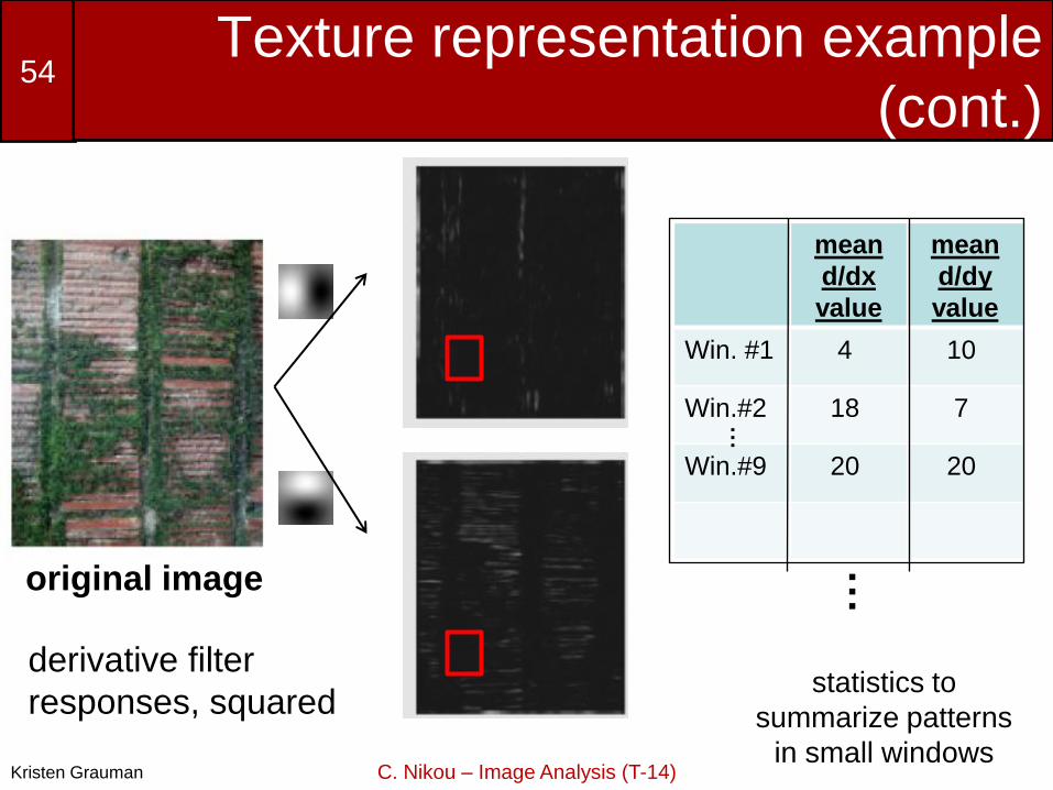
54
C. Nikou – Image Analysis (T-14)
original image
mean
d/dx
value
mean
d/dy
value
Win. #1 4 10
Win.#2 18 7
Win.#9 20 20
…
…
Kristen Grauman
derivative filter
responses, squaredstatistics to
summarize patterns
in small windows
Texture representation example
(cont.)
55
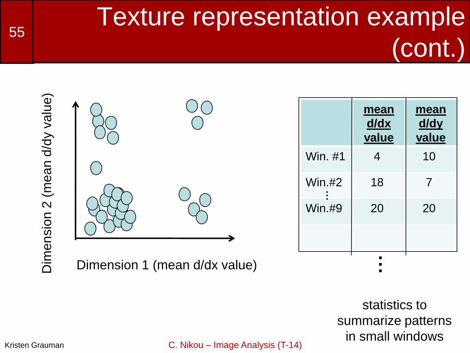
C. Nikou – Image Analysis (T-14)
mean
d/dx
value
mean
d/dy
value
Win. #1 4 10
Win.#2 18 7
Win.#9 20 20
…
…
Dimension 1 (mean d/dx value)Dim
en
sio
n 2
(m
ea
n d
/dy v
alu
e)
Kristen Grauman
Texture representation example
(cont.)
statistics to
summarize patterns
in small windows
56
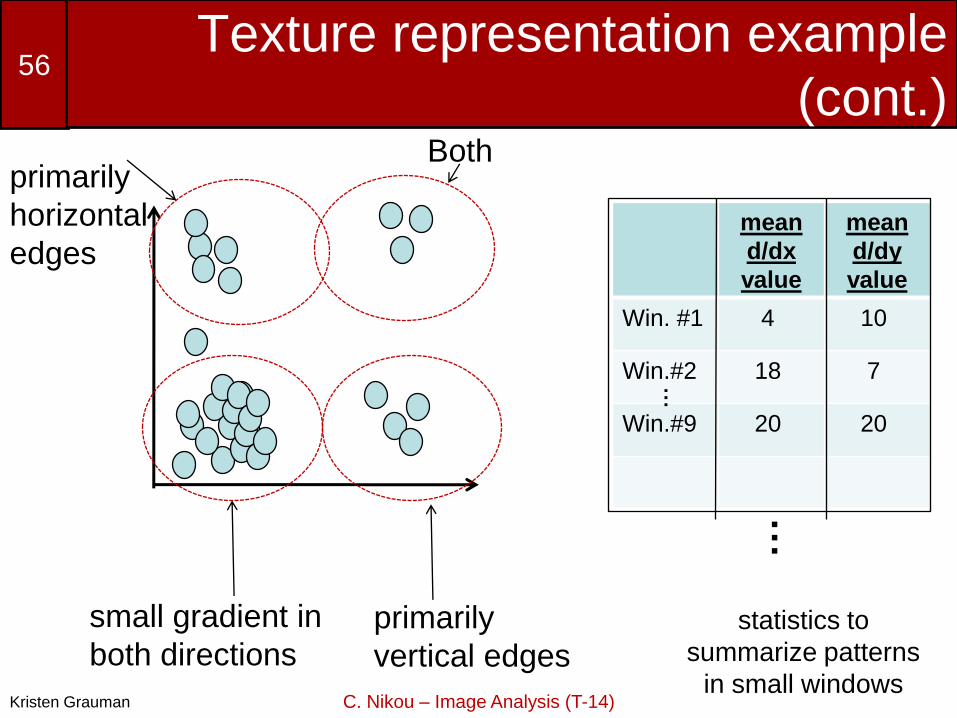
C. Nikou – Image Analysis (T-14)
mean
d/dx
value
mean
d/dy
value
Win. #1 4 10
Win.#2 18 7
Win.#9 20 20
…
…
small gradient in
both directionsprimarily
vertical edges
primarily
horizontal
edges
Both
Kristen Grauman
Texture representation example
(cont.)
statistics to
summarize patterns
in small windows
57
C. Nikou – Image Analysis (T-14)
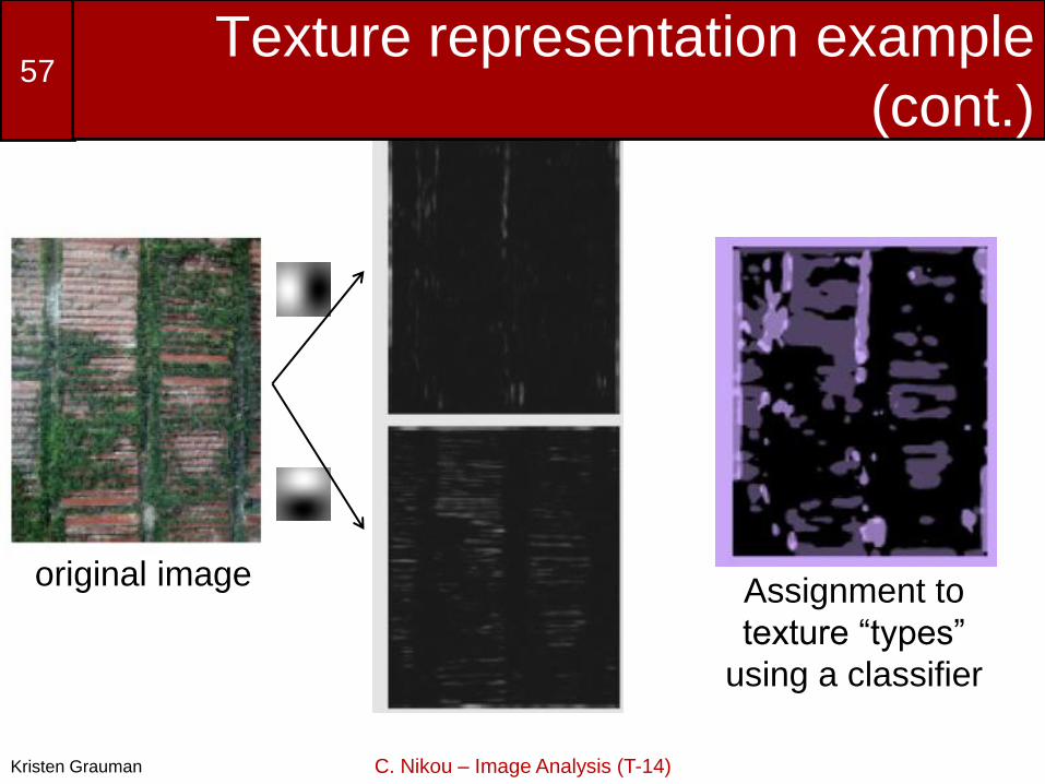
original imageAssignment to
texture ―types‖
using a classifier
Kristen Grauman
Texture representation example
(cont.)
58
C. Nikou – Image Analysis (T-14)
What Statistics? (cont.)
• The choice of statistics depends on what we
represent.
– The mean of the image window and the squared filter
outputs of a filter bank are stacked in a vector
representing an image window (J. Malik and P. Perona,
CVPR 1989).
• This is the method used in the previous example but with a richer
filter bank.
– The mean and standard deviation of filter outputs over the
image window may also be the elements of a feature
vector (W. Ma and B. Manjunath, CVPR 1996).
• Useful for recovery of image windows based on examples
(application to satellite images to determine buildings, vegetation
etc.).
59
C. Nikou – Image Analysis (T-14)
What Statistics? (cont.)
• However, neither mean and standard deviation is
ideal because filter outputs may be similar.
– Small spots arranged in stripes (field of cabbages). Both
spot and bar filters will respond strongly but the responses
are correlated (they respond at the same location).
– On the other hand, if an image contains many large bars
scattered with spots as background the bar and spot filters
will indicate strong uncorrelated responses.
– We could try to record the covariance of the filter outputs
but there are many terms to handle (the dimensionality
increases). This should be done in a limited extent at
certain applications.
60
C. Nikou – Image Analysis (T-14)
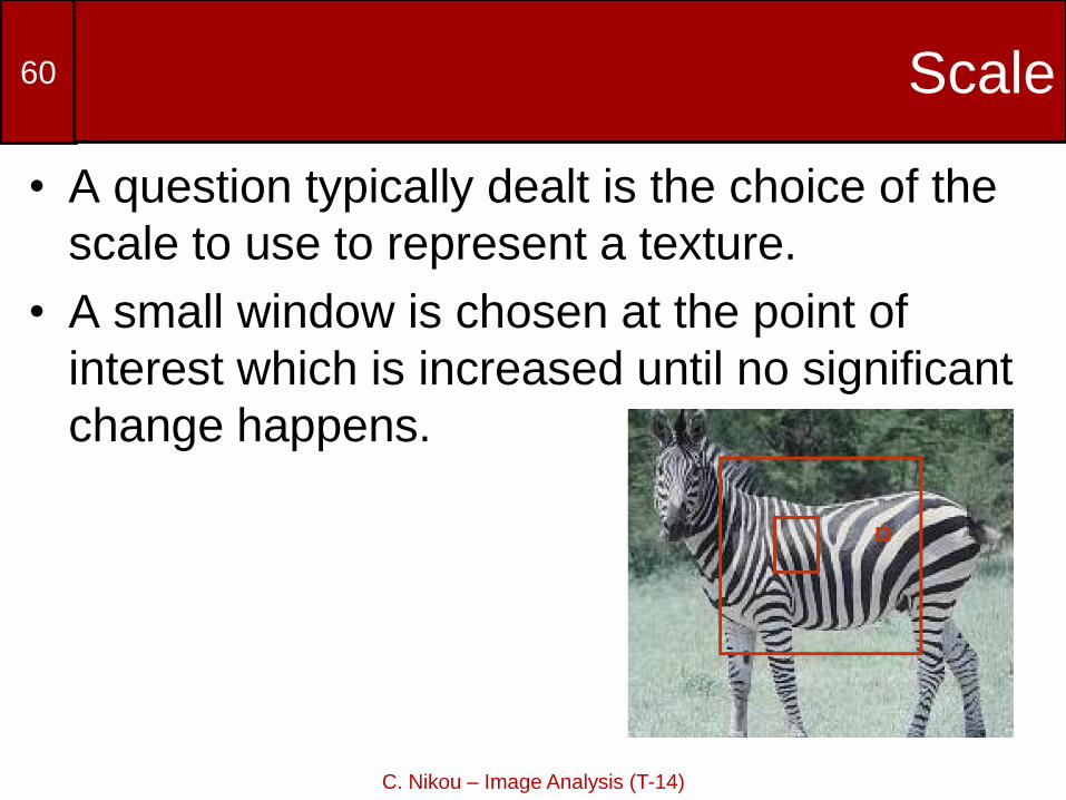
Scale
• A question typically dealt is the choice of the
scale to use to represent a texture.
• A small window is chosen at the point of
interest which is increased until no significant
change happens.
61
C. Nikou – Image Analysis (T-14)
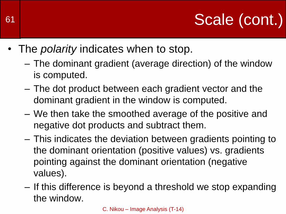
Scale (cont.)
• The polarity indicates when to stop.
– The dominant gradient (average direction) of the window
is computed.
– The dot product between each gradient vector and the
dominant gradient in the window is computed.
– We then take the smoothed average of the positive and
negative dot products and subtract them.
– This indicates the deviation between gradients pointing to
the dominant orientation (positive values) vs. gradients
pointing against the dominant orientation (negative
values).
– If this difference is beyond a threshold we stop expanding
the window.
62
C. Nikou – Image Analysis (T-14)
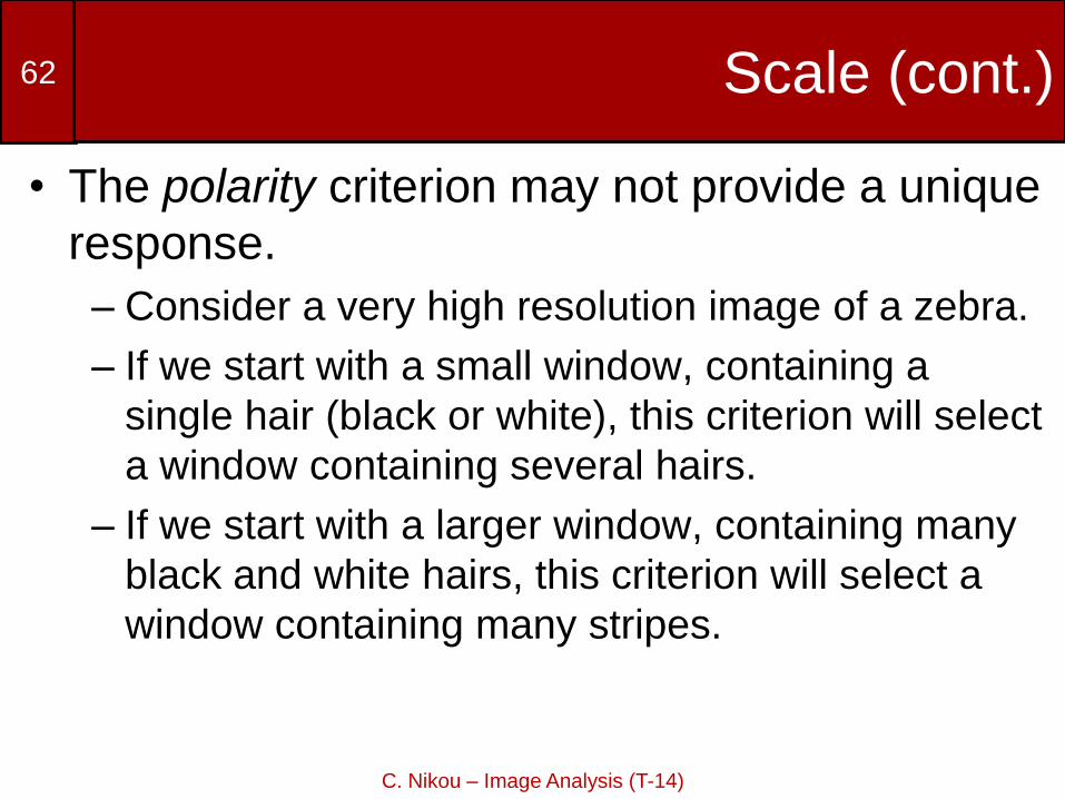
Scale (cont.)
• The polarity criterion may not provide a unique
response.
– Consider a very high resolution image of a zebra.
– If we start with a small window, containing a
single hair (black or white), this criterion will select
a window containing several hairs.
– If we start with a larger window, containing many
black and white hairs, this criterion will select a
window containing many stripes.
63
C. Nikou – Image Analysis (T-14)
Texture Analysis using Oriented
Pyramids• Obtaining filter outputs requires convolution.
• This may be done systematically through pyramids.
• The process of convolving an image with a filter bank
(series of filters) is called analysis.
– Convolution with oriented filters is called analyzing
orientation.
• The Gaussian pyramid is an example of systematic
analysis using smoothing filters of increasing scale.
• Moving from one scale to another is easy as we do
not process redundant information.
64
C. Nikou – Image Analysis (T-14)
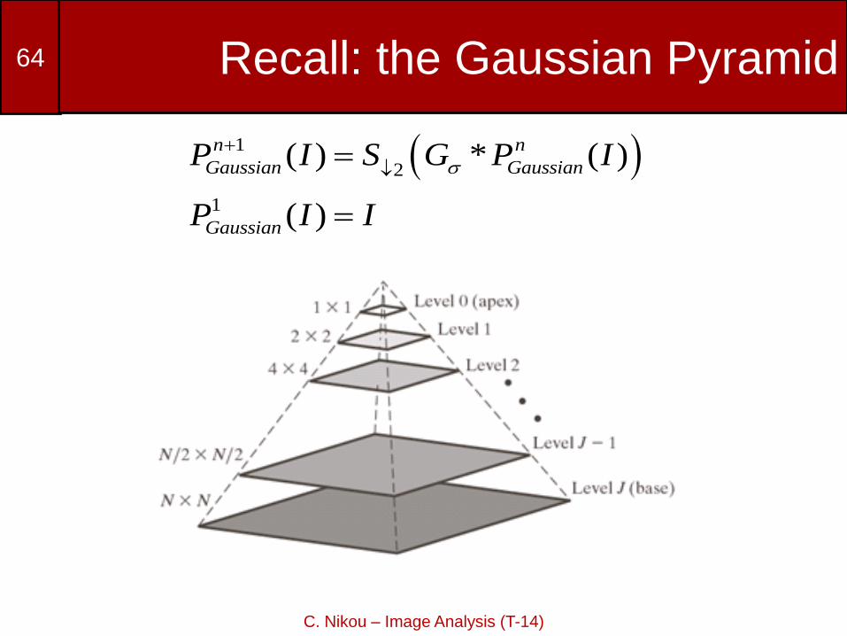
Recall: the Gaussian Pyramid
1
2
1
( ) * ( )
( )
n n
Gaussian Gaussian
Gaussian
P I S G P I
P I I
65
C. Nikou – Image Analysis (T-14)
Recall: the Gaussian Pyramid (cont.)
• Redundant representation: each layer is a low
pass version of the previous layer.
– Low spatial frequencies are represented many
times.
– A layer is a prediction of the next layer. It is not
exact but we know what to expect.
• The Laplacian pyramid keeps only the
prediction errors at each layer.
– Low redundancy.
– It doesn’t deal immediately with orientation.
66
C. Nikou – Image Analysis (T-14)
The Laplacian Pyramid
• A Gaussian pyramid is computed.
• The coarsest layer of the Gaussian
pyramid is also the coarsest layer of the
Laplacian pyramid.
• At each layer, an upsampling operator
produces the image of the finer layer by
row and line duplication.
• The differences of the prediction error are
then stored at the Laplacian pyramid
layers.
67
C. Nikou – Image Analysis (T-14)
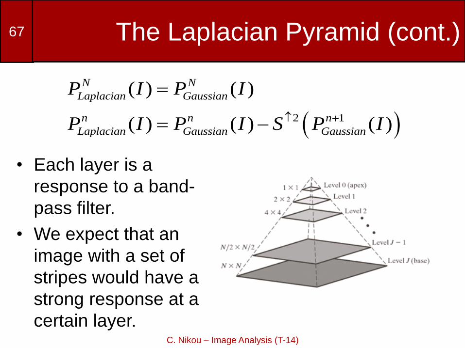
The Laplacian Pyramid (cont.)
• Each layer is a
response to a band-
pass filter.
• We expect that an
image with a set of
stripes would have a
strong response at a
certain layer.
2 1
( ) ( )
( ) ( ) ( )
N N
Laplacian Gaussian
n n n
Laplacian Gaussian Gaussian
P I P I
P I P I S P I
68
C. Nikou – Image Analysis (T-14)
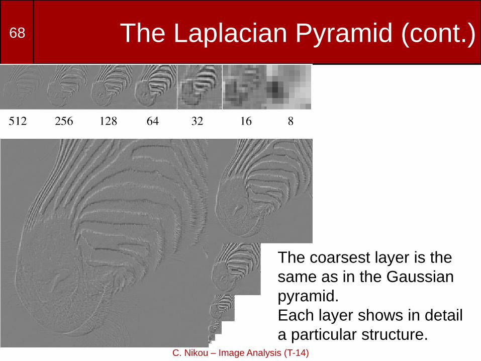
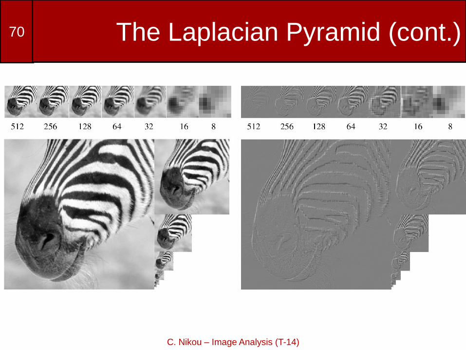
The Laplacian Pyramid (cont.)
The coarsest layer is the
same as in the Gaussian
pyramid.
Each layer shows in detail
a particular structure.
69
C. Nikou – Image Analysis (T-14)
The Laplacian Pyramid (cont.)
• The original image may be reconstructed by the Laplacian
pyramid by first recovering the Gaussian pyramid and
taking the finest layer:
• Algorithm
• Copy the coarsest layer of the Laplacian pyramid to the
coarsest layer of the Gaussian pyramid.
• For each layer, from coarsest to finest of the Laplacian
pyramid
• Upsample it and add the result to the next layer of the pyramid.
70
C. Nikou – Image Analysis (T-14)
The Laplacian Pyramid (cont.)
71
C. Nikou – Image Analysis (T-14)
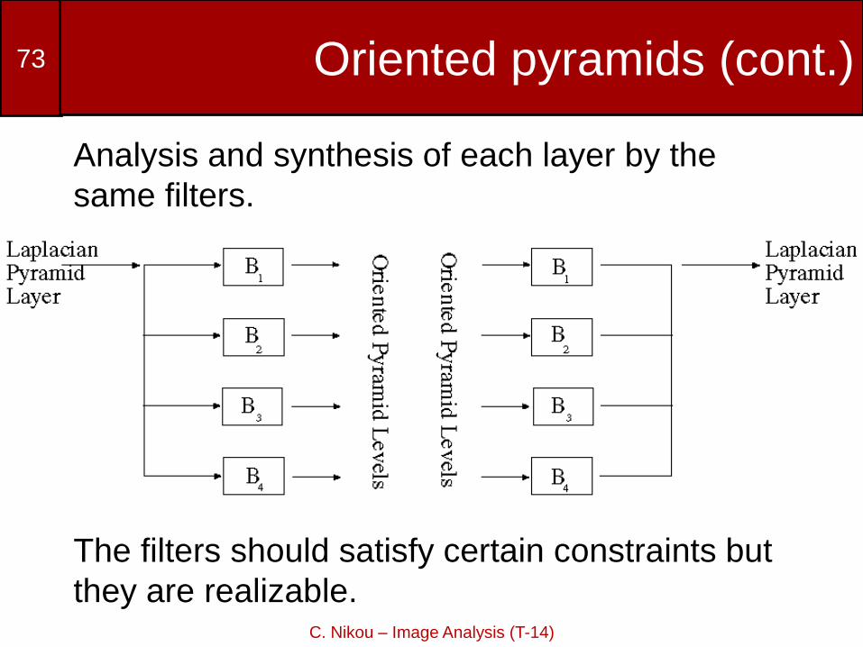
Oriented pyramids
• The Laplacian pyramid encodes frequency but it
does not contain information about texture
orientation.
• We may further decompose each layer by
oriented filters providing an oriented pyramid.
• Design constraint: synthesis should be easy.
– It is possible to design filters where synthesis at each
layer may be obtained by filtering the layer
components by the same analysis filters a second
time (Simoncelli and Freeman, ICIP 1995).
72
C. Nikou – Image Analysis (T-14)
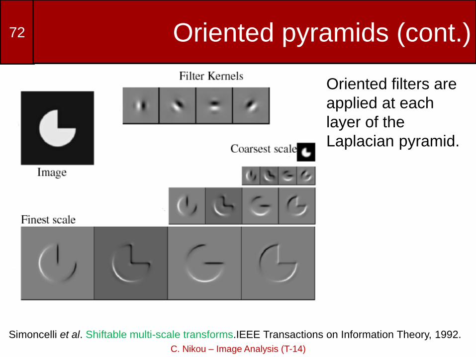
Oriented pyramids (cont.)
Simoncelli et al. Shiftable multi-scale transforms.IEEE Transactions on Information Theory, 1992.
Oriented filters are
applied at each
layer of the
Laplacian pyramid.
73
C. Nikou – Image Analysis (T-14)
Oriented pyramids (cont.)
Analysis and synthesis of each layer by the
same filters.
The filters should satisfy certain constraints but
they are realizable.
74
C. Nikou – Image Analysis (T-14)
Gabor Filters
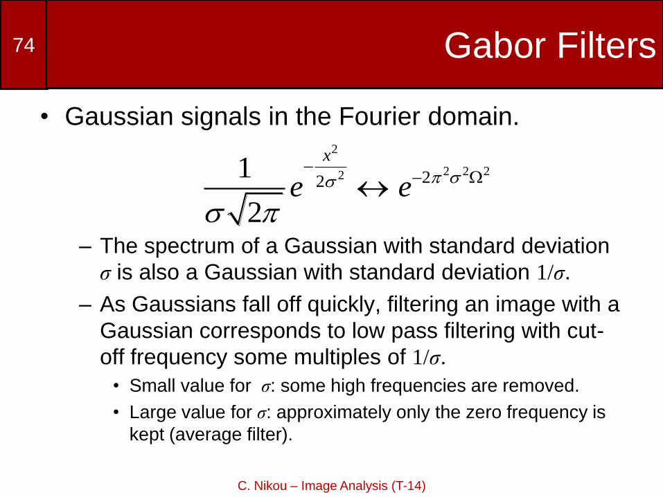
• Gaussian signals in the Fourier domain.
– The spectrum of a Gaussian with standard deviation
σ is also a Gaussian with standard deviation 1/σ.
– As Gaussians fall off quickly, filtering an image with a
Gaussian corresponds to low pass filtering with cut-
off frequency some multiples of 1/σ.
• Small value for σ: some high frequencies are removed.
• Large value for σ: approximately only the zero frequency is
kept (average filter).
2
2 2 22 221
2
x
e e
75
C. Nikou – Image Analysis (T-14)
Gabor Filters (cont.)
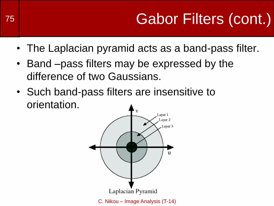
• The Laplacian pyramid acts as a band-pass filter.
• Band –pass filters may be expressed by the
difference of two Gaussians.
• Such band-pass filters are insensitive to
orientation.
76
C. Nikou – Image Analysis (T-14)
Gabor Filters (cont.)
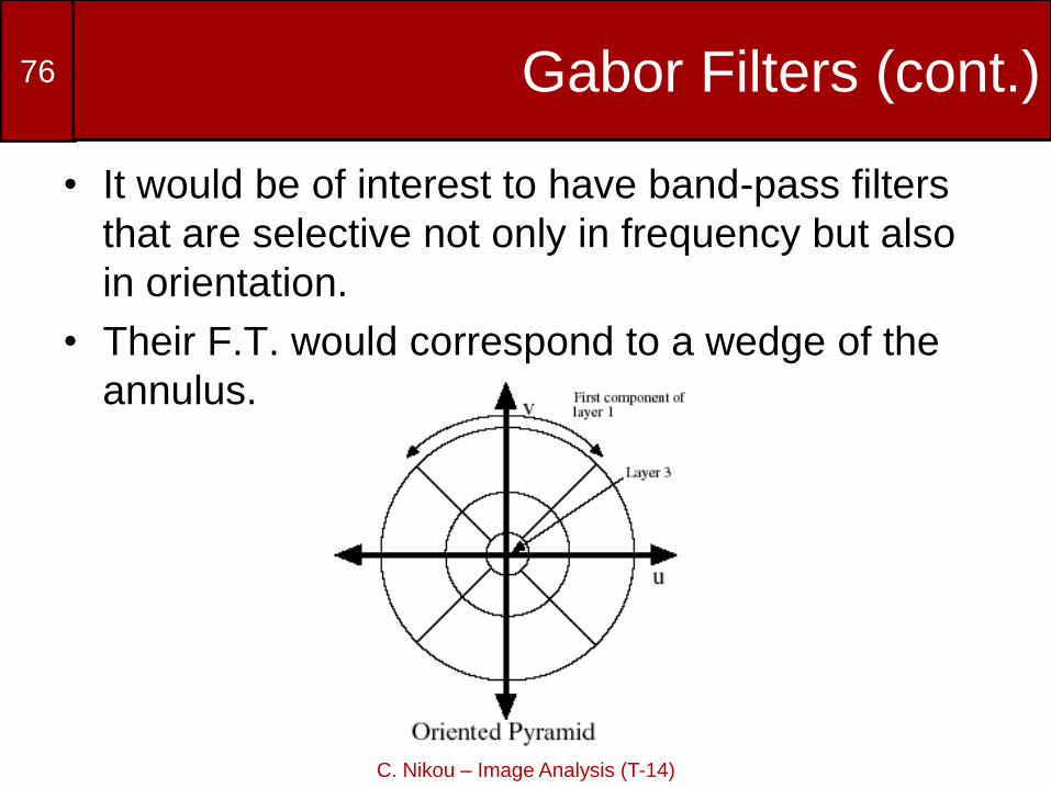
• It would be of interest to have band-pass filters
that are selective not only in frequency but also
in orientation.
• Their F.T. would correspond to a wedge of the
annulus.
77
C. Nikou – Image Analysis (T-14)
Gabor Filters (cont.)
• How can we obtain these wedges?
• Sinusoids have spectrum of Dirac functions.
• They may guide the spectral signature to a wedge.
• Difficulty in representing local texture:
– The value of the FT at a particular frequency needs
integration of the whole image data.
– FT is not location-selective.
• We have to enforce the FT to be selective in
location.
– The Gaussian function will help us as it cuts off its
support depending on the value of σ.
78
C. Nikou – Image Analysis (T-14)
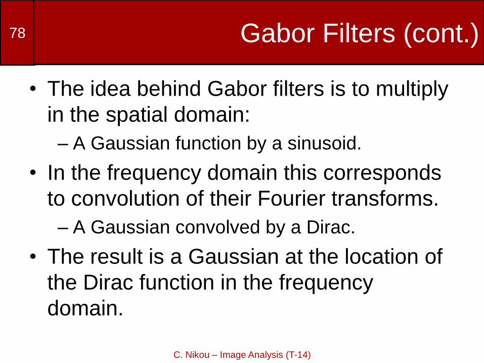
Gabor Filters (cont.)
• The idea behind Gabor filters is to multiply
in the spatial domain:
– A Gaussian function by a sinusoid.
• In the frequency domain this corresponds
to convolution of their Fourier transforms.
– A Gaussian convolved by a Dirac.
• The result is a Gaussian at the location of
the Dirac function in the frequency
domain.
79
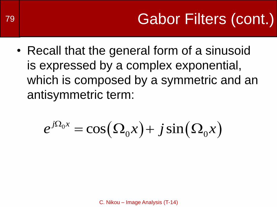
C. Nikou – Image Analysis (T-14)
Gabor Filters (cont.)
• Recall that the general form of a sinusoid
is expressed by a complex exponential,
which is composed by a symmetric and an
antisymmetric term:
0
0 0cos sinj x
e x j x
80
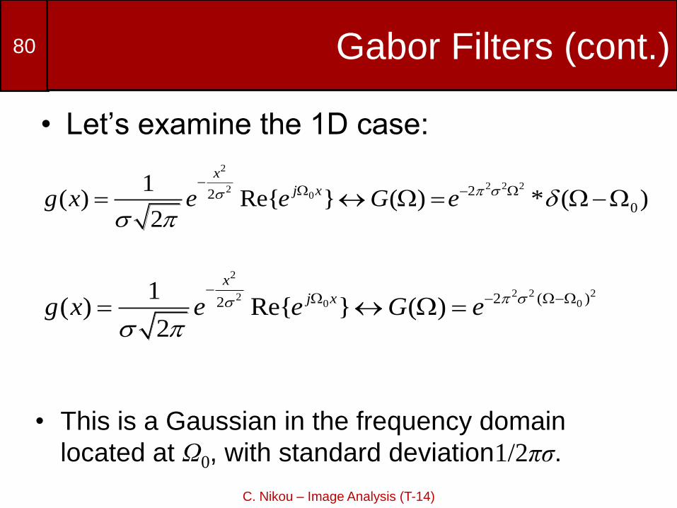
C. Nikou – Image Analysis (T-14)
Gabor Filters (cont.)
• Let’s examine the 1D case:
2
2 2 220 22
0
1( ) Re{ } ( ) * ( )
2
x
j xg x e e G e
2
2 2 220 02 ( )2
1( ) Re{ } ( )
2
x
j xg x e e G e
• This is a Gaussian in the frequency domain
located at Ω0, with standard deviation1/2πσ.
81
C. Nikou – Image Analysis (T-14)
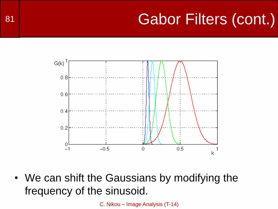
Gabor Filters (cont.)
• We can shift the Gaussians by modifying the
frequency of the sinusoid.
82
C. Nikou – Image Analysis (T-14)
Gabor Filters (cont.)
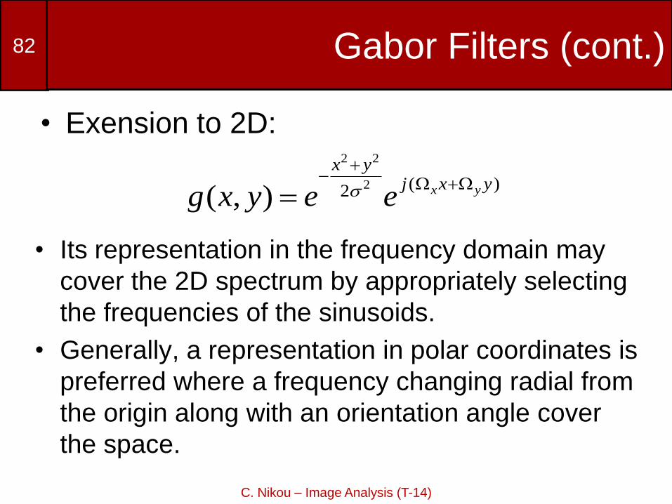
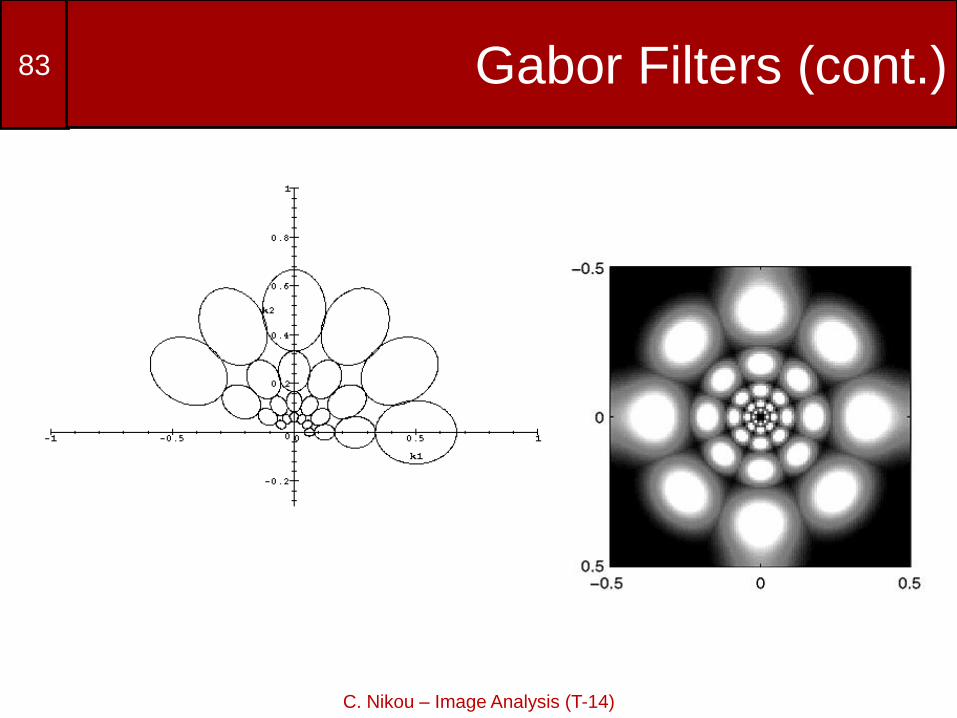
• Exension to 2D:2 2
2 ( )2( , ) x y
x yj x y
g x y e e
• Its representation in the frequency domain may
cover the 2D spectrum by appropriately selecting
the frequencies of the sinusoids.
• Generally, a representation in polar coordinates is
preferred where a frequency changing radial from
the origin along with an orientation angle cover
the space.
83
C. Nikou – Image Analysis (T-14)
Gabor Filters (cont.)
84
C. Nikou – Image Analysis (T-14)
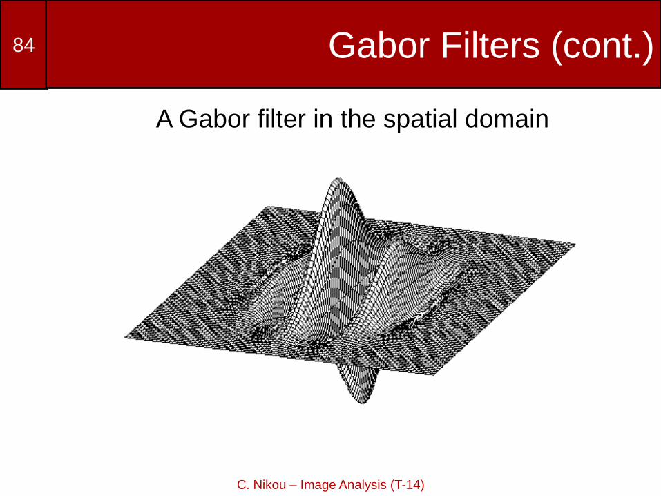
Gabor Filters (cont.)
A Gabor filter in the spatial domain
85
C. Nikou – Image Analysis (T-14)
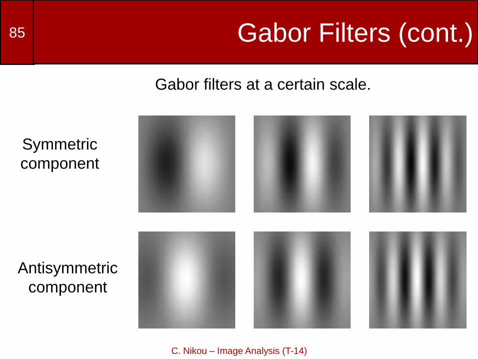
Gabor Filters (cont.)
Gabor filters at a certain scale.
Symmetric
component
Antisymmetric
component
86
C. Nikou – Image Analysis (T-14)
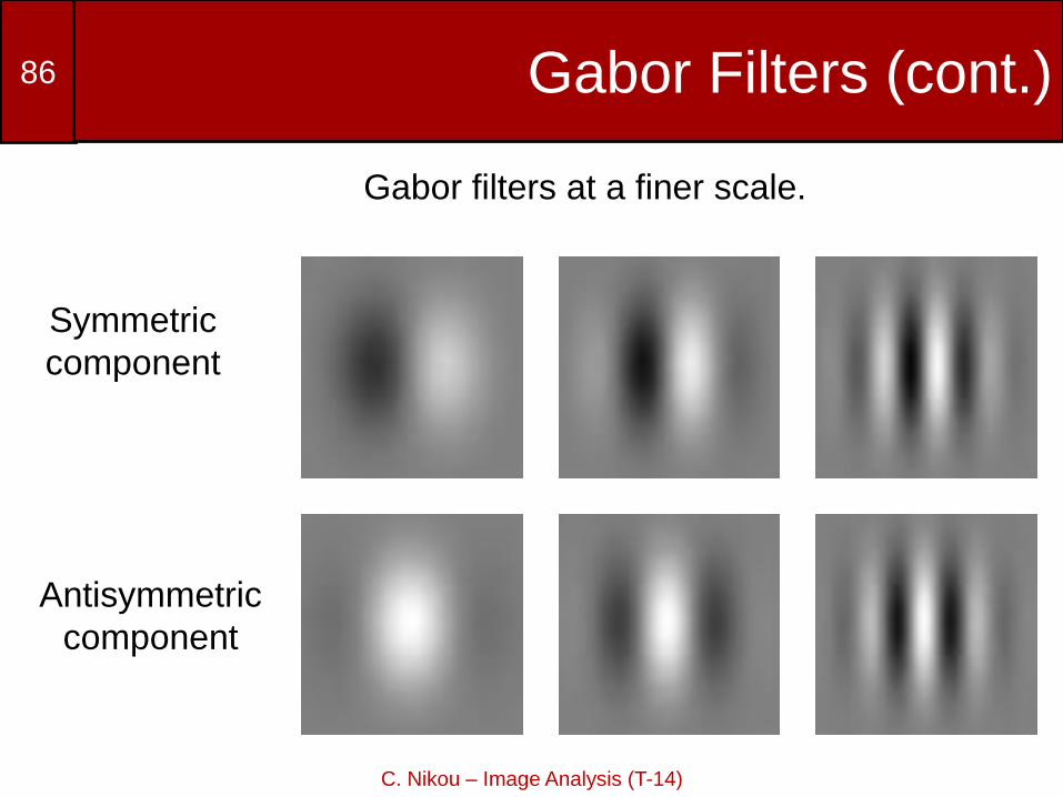
Gabor Filters (cont.)
Gabor filters at a finer scale.
Symmetric
component
Antisymmetric
component
87
C. Nikou – Image Analysis (T-14)
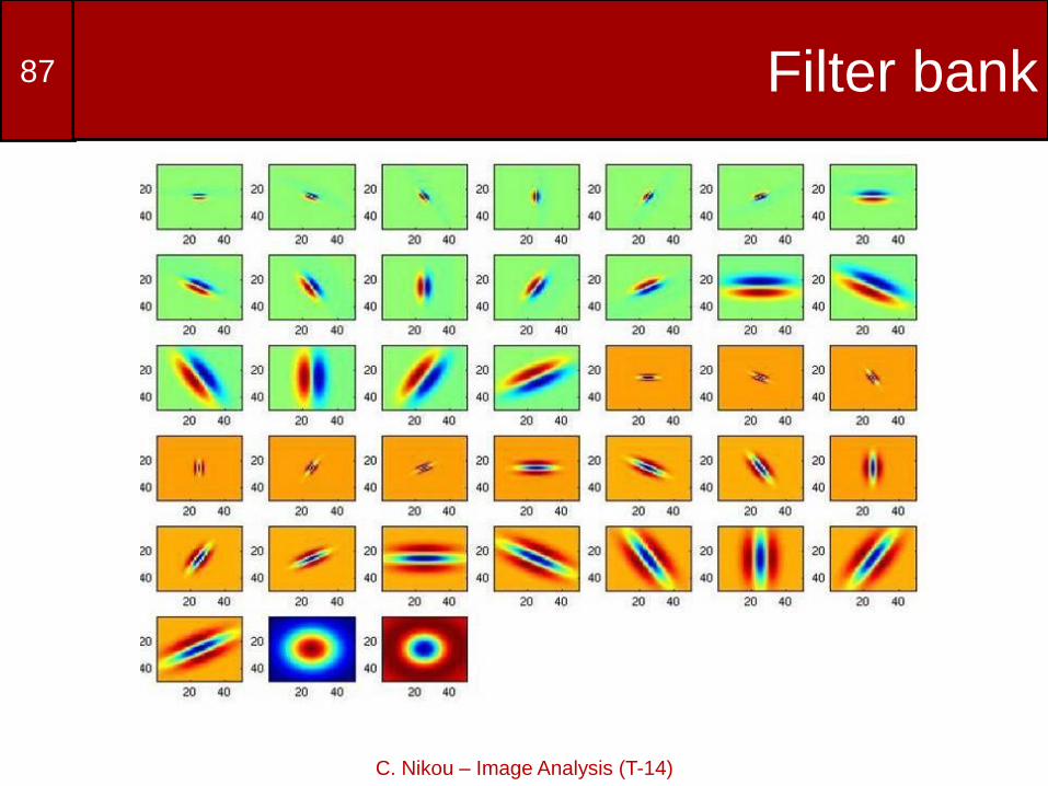
Filter bank
88
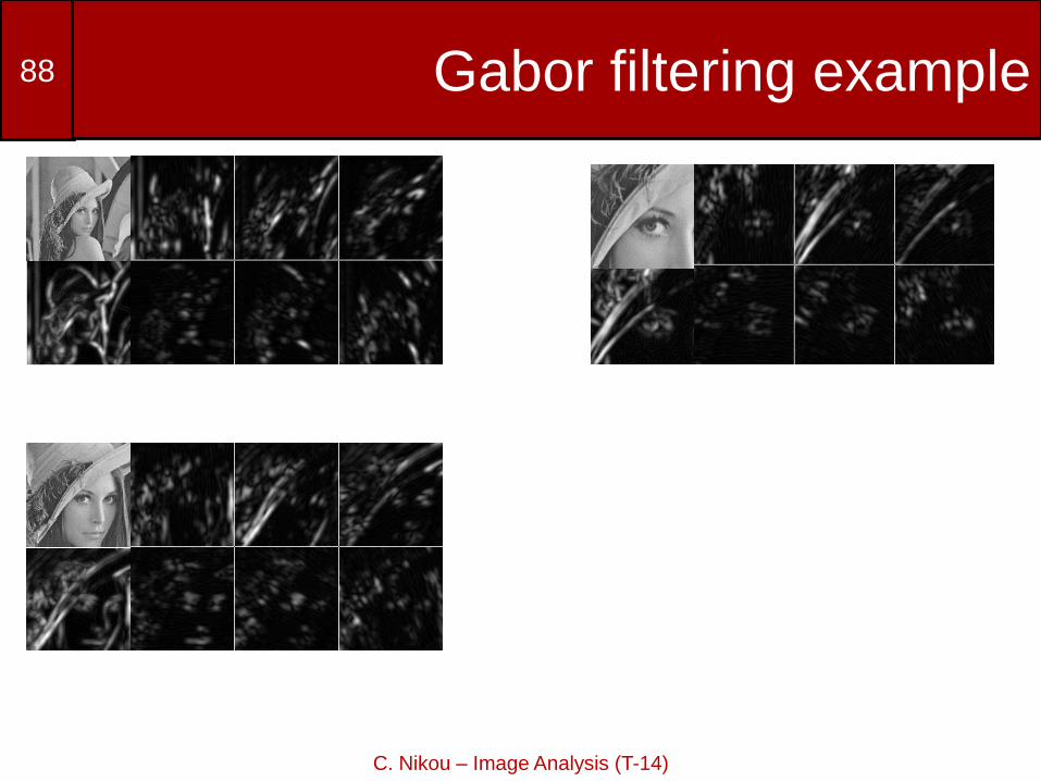
C. Nikou – Image Analysis (T-14)
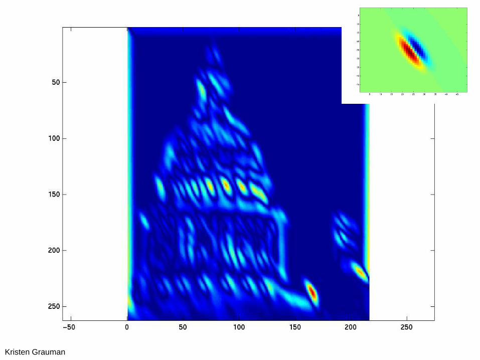
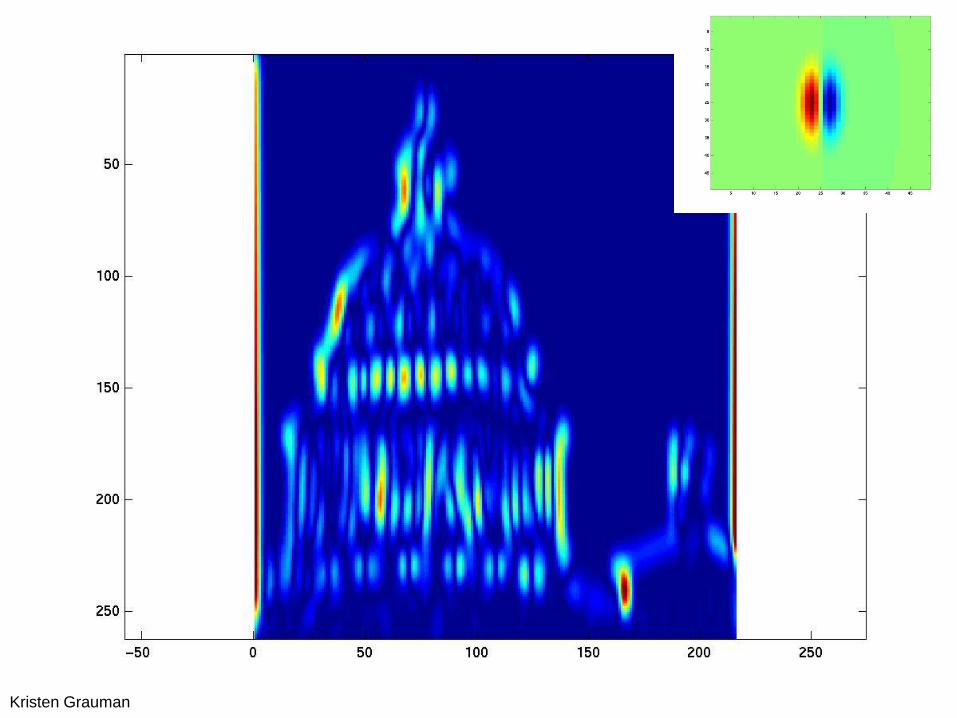
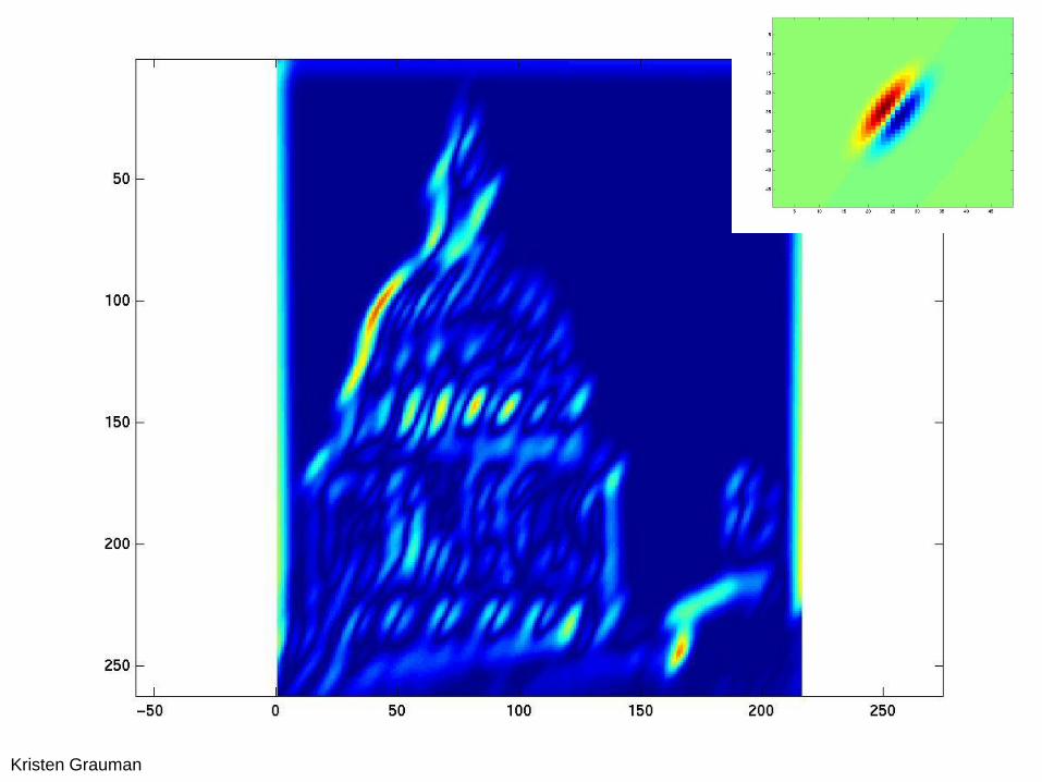
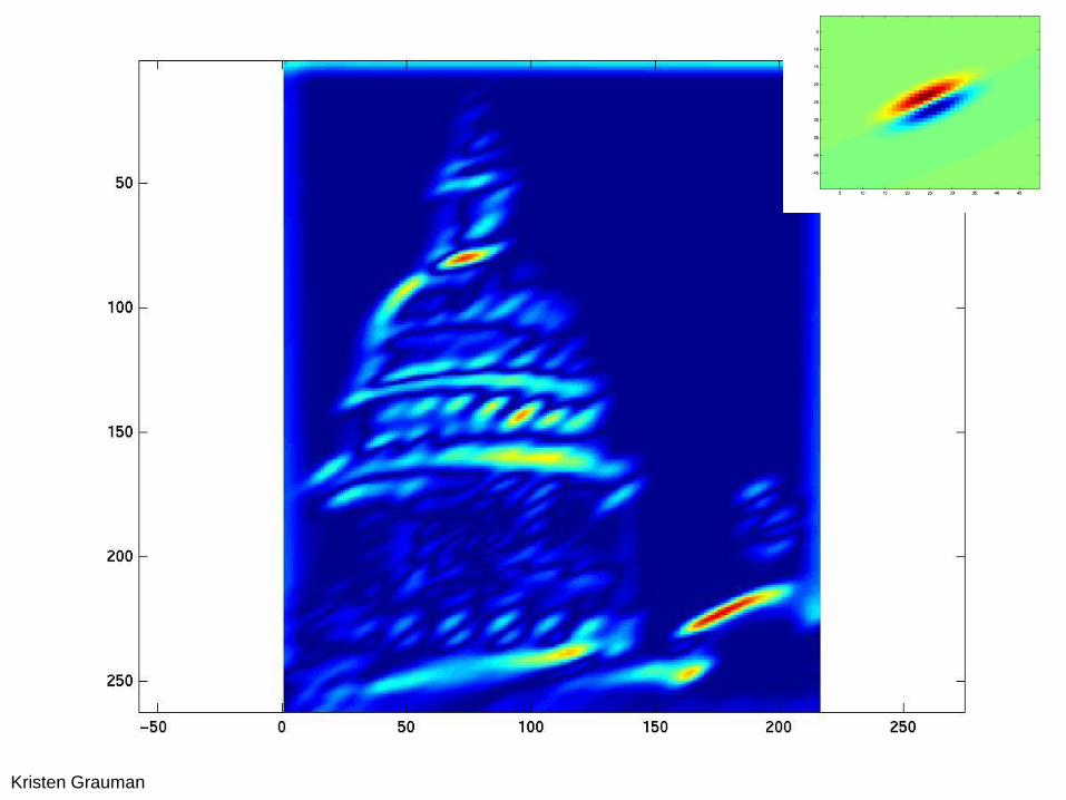
Gabor filtering example
89
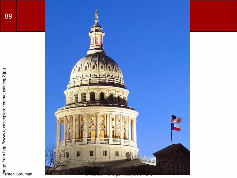
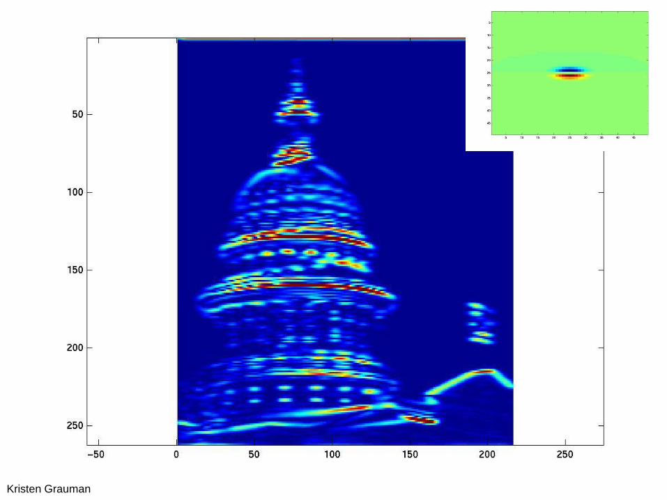
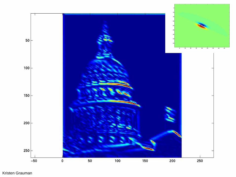
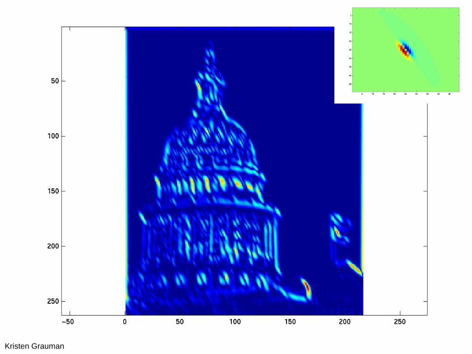
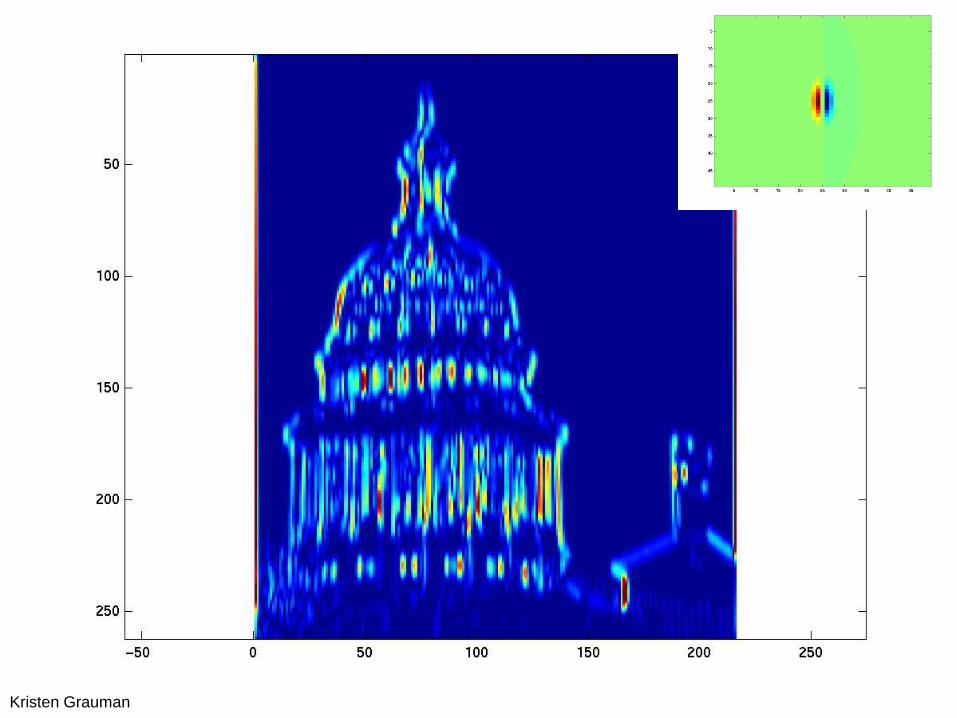
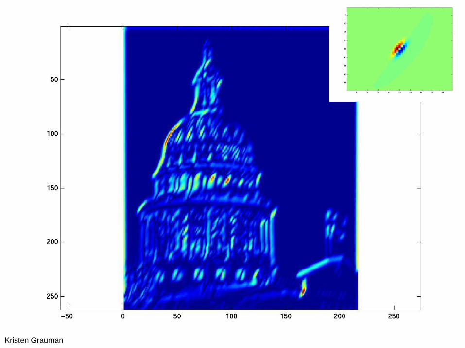
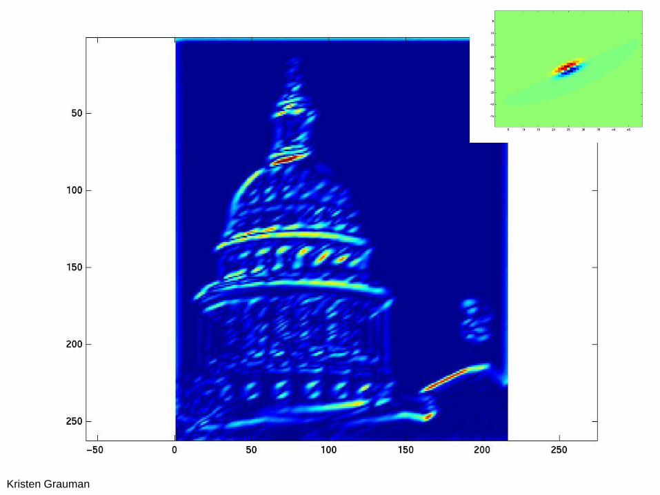
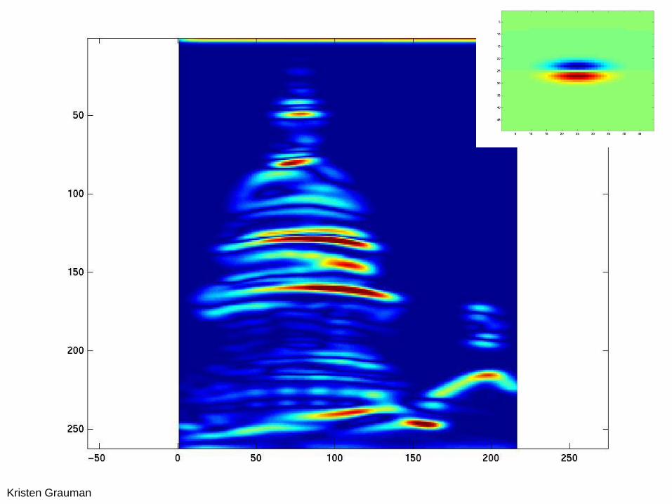
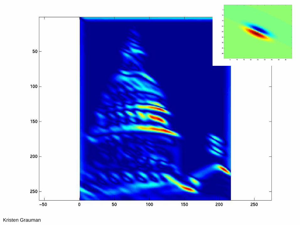
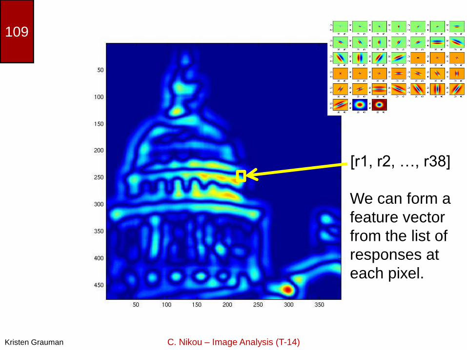
C. Nikou – Image Analysis (T-14)Image f
rom
http://w
ww
.te
xase
xplo
rer.com
/austincap2
.jpg
Kristen Grauman
90
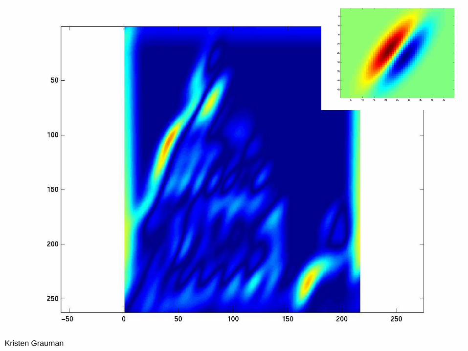
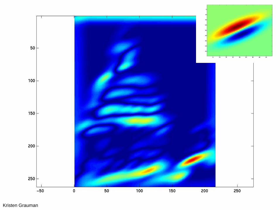
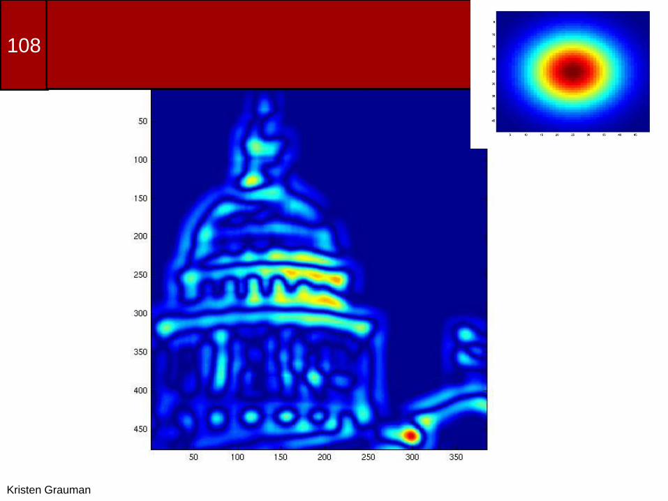
C. Nikou – Image Analysis (T-14)
Showing magnitude of
responses
Kristen Grauman
91
C. Nikou – Image Analysis (T-14)Kristen Grauman
92
C. Nikou – Image Analysis (T-14)Kristen Grauman
93
C. Nikou – Image Analysis (T-14)Kristen Grauman
94
C. Nikou – Image Analysis (T-14)Kristen Grauman
95
C. Nikou – Image Analysis (T-14)Kristen Grauman
96
C. Nikou – Image Analysis (T-14)Kristen Grauman
97
C. Nikou – Image Analysis (T-14)Kristen Grauman
98
C. Nikou – Image Analysis (T-14)Kristen Grauman
99
C. Nikou – Image Analysis (T-14)Kristen Grauman
100
C. Nikou – Image Analysis (T-14)Kristen Grauman
101
C. Nikou – Image Analysis (T-14)Kristen Grauman
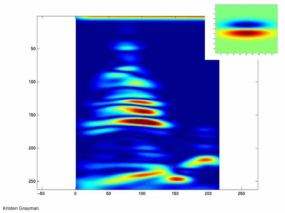
102
C. Nikou – Image Analysis (T-14)Kristen Grauman
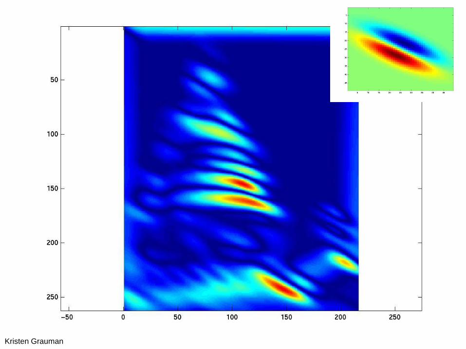
103
C. Nikou – Image Analysis (T-14)Kristen Grauman
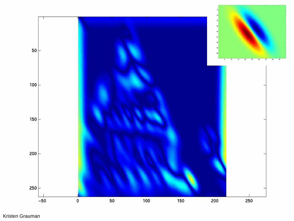
104
C. Nikou – Image Analysis (T-14)Kristen Grauman
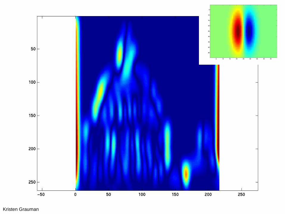
105
C. Nikou – Image Analysis (T-14)Kristen Grauman
106
C. Nikou – Image Analysis (T-14)Kristen Grauman
107
C. Nikou – Image Analysis (T-14)Kristen Grauman
108
C. Nikou – Image Analysis (T-14)Kristen Grauman
109
C. Nikou – Image Analysis (T-14)
[r1, r2, …, r38]
We can form a
feature vector
from the list of
responses at
each pixel.
Kristen Grauman
110
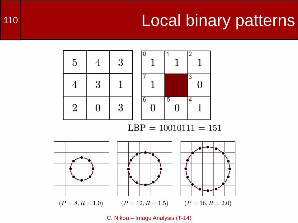
C. Nikou – Image Analysis (T-14)
Local binary patterns
111
C. Nikou – Image Analysis (T-14)
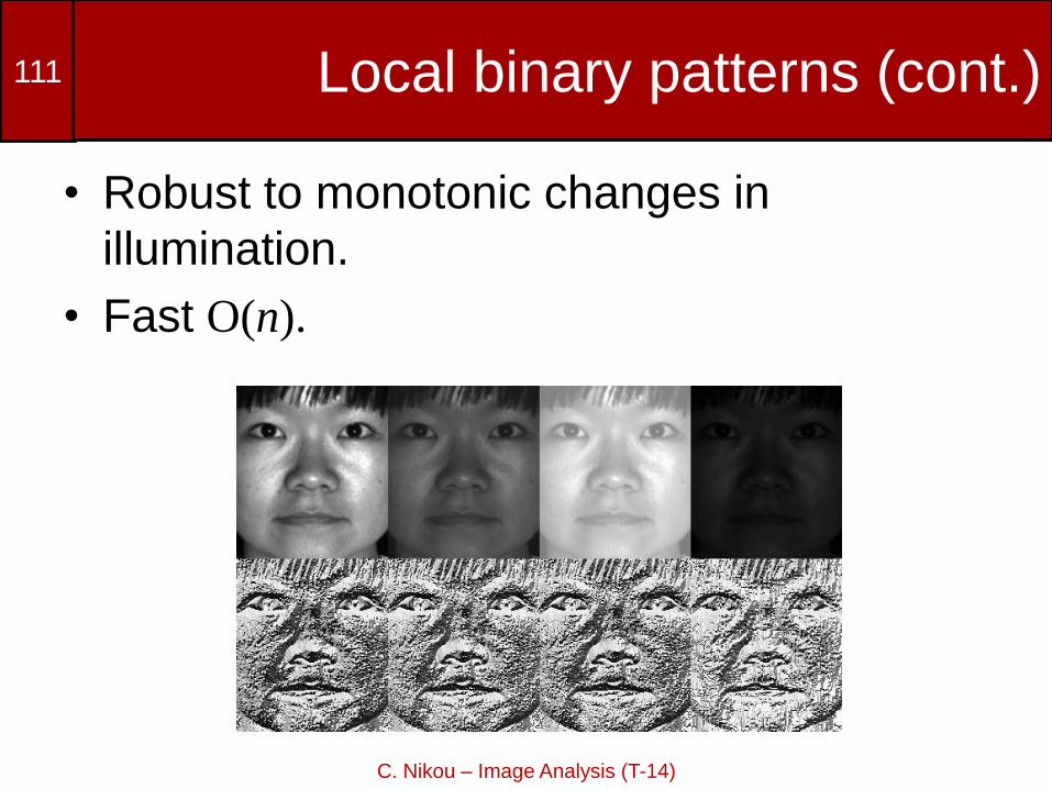
Local binary patterns (cont.)
• Robust to monotonic changes in
illumination.
• Fast O(n).
112
C. Nikou – Image Analysis (T-14)
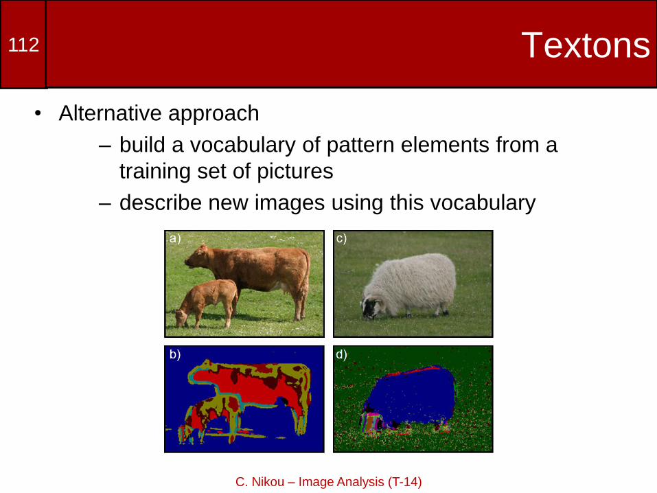
Textons
• Alternative approach
– build a vocabulary of pattern elements from a
training set of pictures
– describe new images using this vocabulary
113
C. Nikou – Image Analysis (T-14)
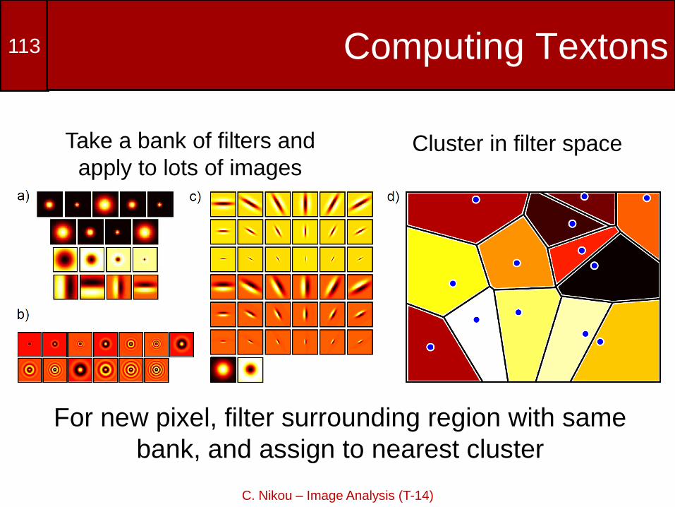
Computing Textons
Take a bank of filters and
apply to lots of imagesCluster in filter space
For new pixel, filter surrounding region with same
bank, and assign to nearest cluster
114
C. Nikou – Image Analysis (T-14)
Textons
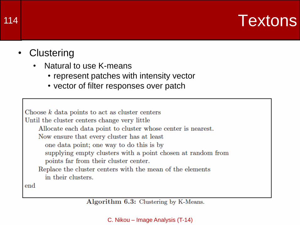
• Clustering
• Natural to use K-means
• represent patches with intensity vector
• vector of filter responses over patch
115
C. Nikou – Image Analysis (T-14)
Textons
116
C. Nikou – Image Analysis (T-14)
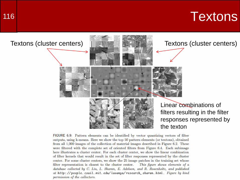
Textons
Textons (cluster centers) Textons (cluster centers)
Linear combinations of
filters resulting in the filter
responses represented by
the texton
117
C. Nikou – Image Analysis (T-14)
Texture synthesis
• Application to computer graphics for
texture mapping.
– Rendered objects look more realistic (why?).
• Simple tiling does not work properly.
– Continuity at boundaries.
– The resulting periodic structure may be
visually annoying.
• Possible to buy textures for mapping but
more interesting if we may create them
from example images!
118
C. Nikou – Image Analysis (T-14)
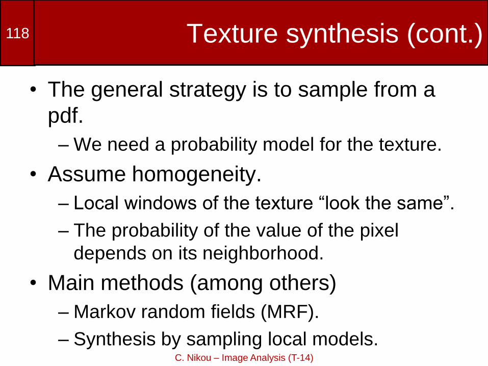
Texture synthesis (cont.)
• The general strategy is to sample from a
pdf.
– We need a probability model for the texture.
• Assume homogeneity.
– Local windows of the texture ―look the same‖.
– The probability of the value of the pixel
depends on its neighborhood.
• Main methods (among others)
– Markov random fields (MRF).
– Synthesis by sampling local models.
119
C. Nikou – Image Analysis (T-14)
Texture modeling by MRF (cont.)
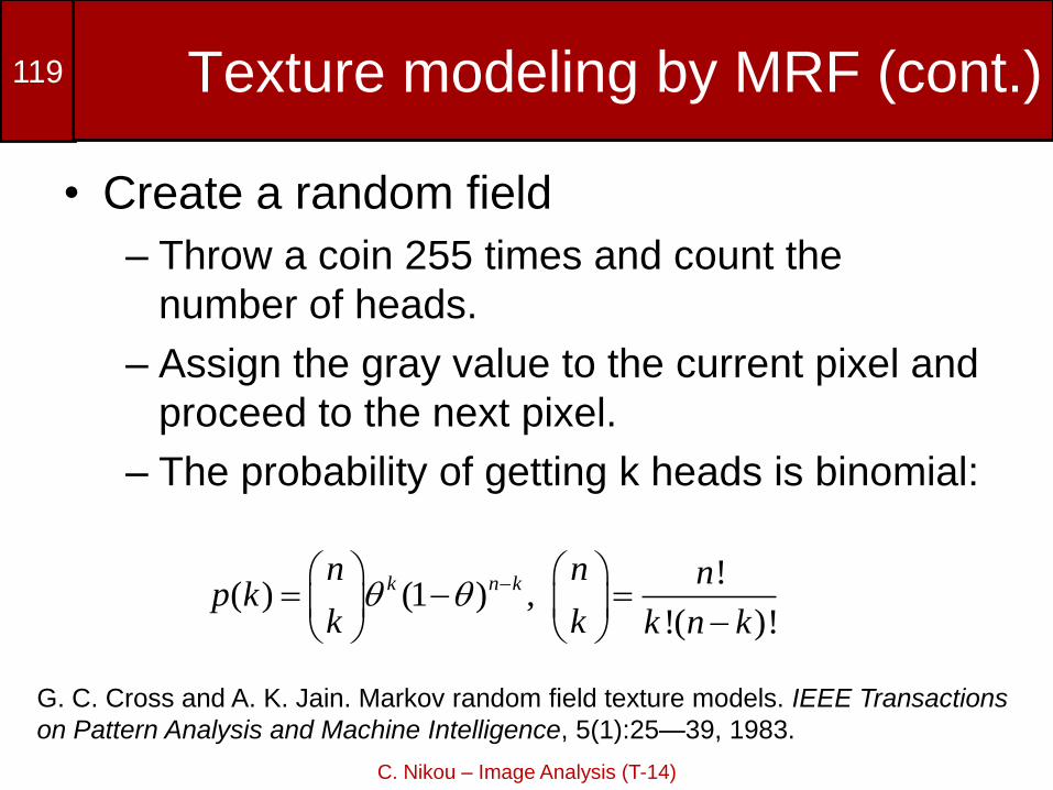
• Create a random field
– Throw a coin 255 times and count the
number of heads.
– Assign the gray value to the current pixel and
proceed to the next pixel.
– The probability of getting k heads is binomial:
!( ) (1 ) ,
!( )!
k n kn n n
p kk k k n k
G. C. Cross and A. K. Jain. Markov random field texture models. IEEE Transactions
on Pattern Analysis and Machine Intelligence, 5(1):25—39, 1983.
120
C. Nikou – Image Analysis (T-14)
Texture modeling by MRF (cont.)
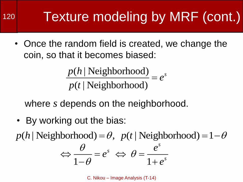
• Once the random field is created, we change the
coin, so that it becomes biased:
( | Neighborhood)
( | Neighborhood)
sp he
p t
• By working out the bias:
( | Neighborhood) , ( | Neighborhood) 1p h p t
1 1
ss
s
ee
e
where s depends on the neighborhood.
121
C. Nikou – Image Analysis (T-14)
Texture modeling by MRF (cont.)
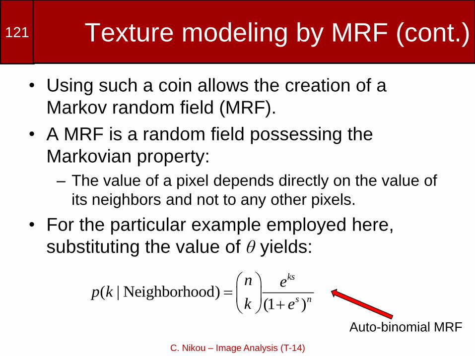
• Using such a coin allows the creation of a
Markov random field (MRF).
• A MRF is a random field possessing the
Markovian property:
– The value of a pixel depends directly on the value of
its neighbors and not to any other pixels.
• For the particular example employed here,
substituting the value of θ yields:
( | Neighborhood)(1 )
ks
s n
n ep k
k e
Auto-binomial MRF
122
C. Nikou – Image Analysis (T-14)
Texture modeling by MRF (cont.)
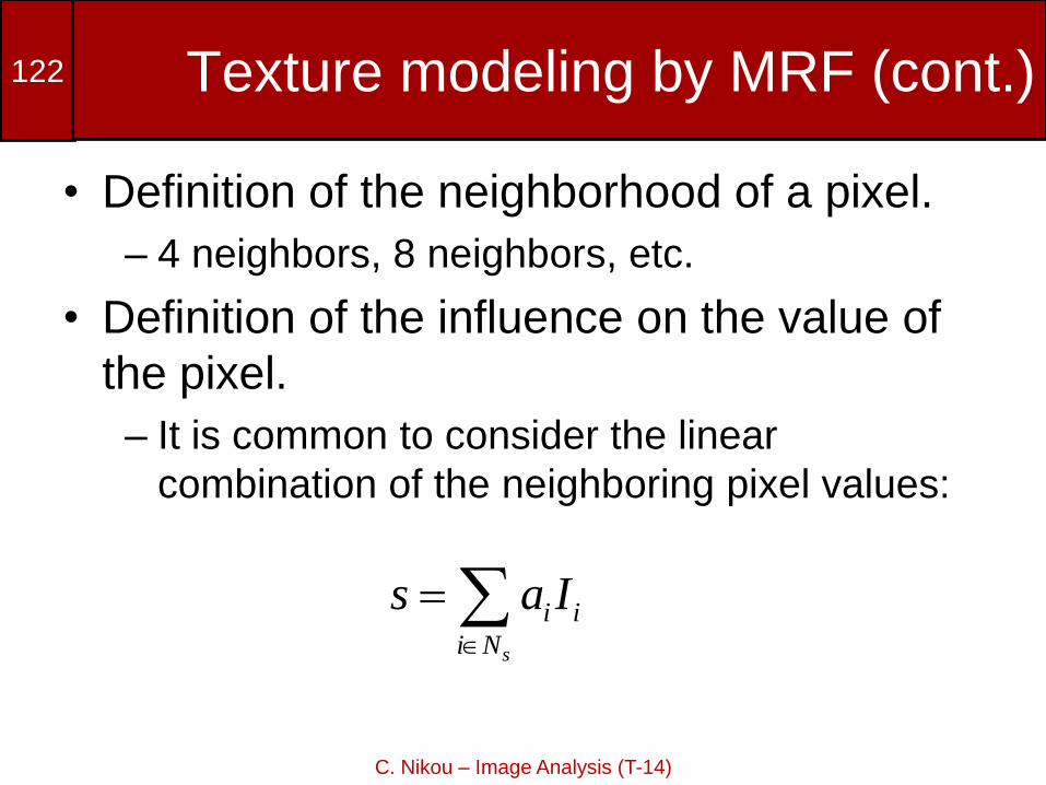
• Definition of the neighborhood of a pixel.
– 4 neighbors, 8 neighbors, etc.
• Definition of the influence on the value of
the pixel.
– It is common to consider the linear
combination of the neighboring pixel values:
s
i i
i N
s a I
123
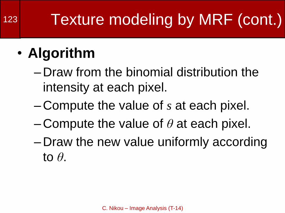
C. Nikou – Image Analysis (T-14)
Texture modeling by MRF (cont.)
• Algorithm
– Draw from the binomial distribution the
intensity at each pixel.
– Compute the value of s at each pixel.
– Compute the value of θ at each pixel.
– Draw the new value uniformly according
to θ.
124
C. Nikou – Image Analysis (T-14)
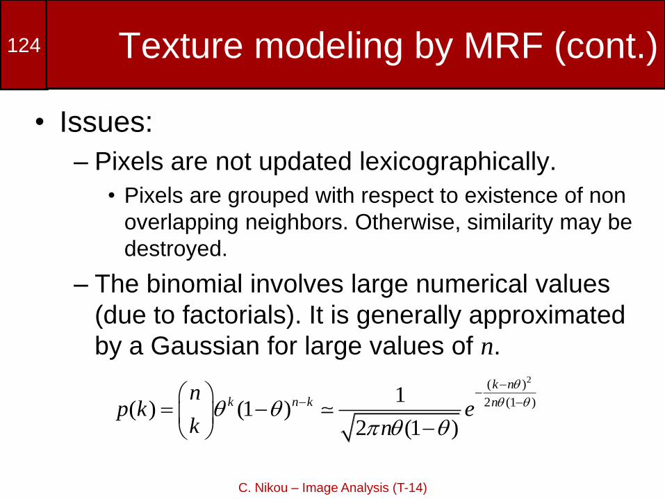
Texture modeling by MRF (cont.)
• Issues:
– Pixels are not updated lexicographically.
• Pixels are grouped with respect to existence of non
overlapping neighbors. Otherwise, similarity may be
destroyed.
– The binomial involves large numerical values
(due to factorials). It is generally approximated
by a Gaussian for large values of n.2( )
2 (1 )1( ) (1 )
2 (1 )
k n
k n k nn
p k ek n
125
C. Nikou – Image Analysis (T-14)
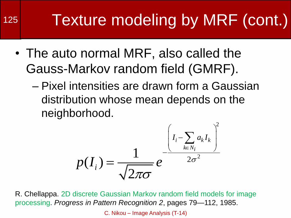
Texture modeling by MRF (cont.)
• The auto normal MRF, also called the
Gauss-Markov random field (GMRF).
– Pixel intensities are drawn form a Gaussian
distribution whose mean depends on the
neighborhood.2
221
( )2
i k k
k Ni
I a I
ip I e
R. Chellappa. 2D discrete Gaussian Markov random field models for image
processing. Progress in Pattern Recognition 2, pages 79—112, 1985.
126
C. Nikou – Image Analysis (T-14)
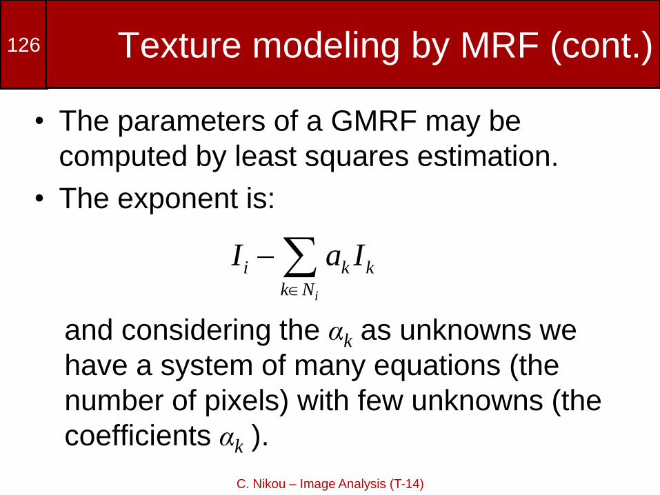
Texture modeling by MRF (cont.)
• The parameters of a GMRF may be
computed by least squares estimation.
• The exponent is:
i
i k k
k N
I a I
and considering the αk as unknowns we
have a system of many equations (the
number of pixels) with few unknowns (the
coefficients αk ).
127
C. Nikou – Image Analysis (T-14)
Texture Synthesis by non-
Parametric Sampling
• We can construct texture outside the
boundaries of an example image.
• The example image can serve as a
probability model.
• This model applies to natural texture over a
reasonable range of scales.
– Stripes on zebra’s body are vertical but they are
horizontal on the legs.
128
C. Nikou – Image Analysis (T-14)
Texture Synthesis by non-
Parametric Sampling (cont.)
• The idea is to take a neighborhood around a
pixel and compare its neighbors to regions in
the example image.
• The size of the neighborhood is significant to
capture large scale details.
• The similarity may be the sum of the
squared differences of the neighbors.
• Only synthesized pixels of the neighborhood
of the pixel to be synthesized count in the
similarity.
129
C. Nikou – Image Analysis (T-14)
Texture Synthesis by non-
Parametric Sampling (cont.)
• Algorithm
– Initialization
• Choose a small square at random from the example
image and insert it into the synthesized image.
– Until all pixels are visited
• For each unvisited pixel on the boundary of the
region of synthesized values
– Match the neighborhood of the pixel to the example image,
ignoring unsynthesized locations and compute a match
criterion.
– Choose the value at random from the set of values of the
example image where the criterion is less than a threshold.
130
C. Nikou – Image Analysis (T-14)
Texture Synthesis by non-
Parametric Sampling (cont.)
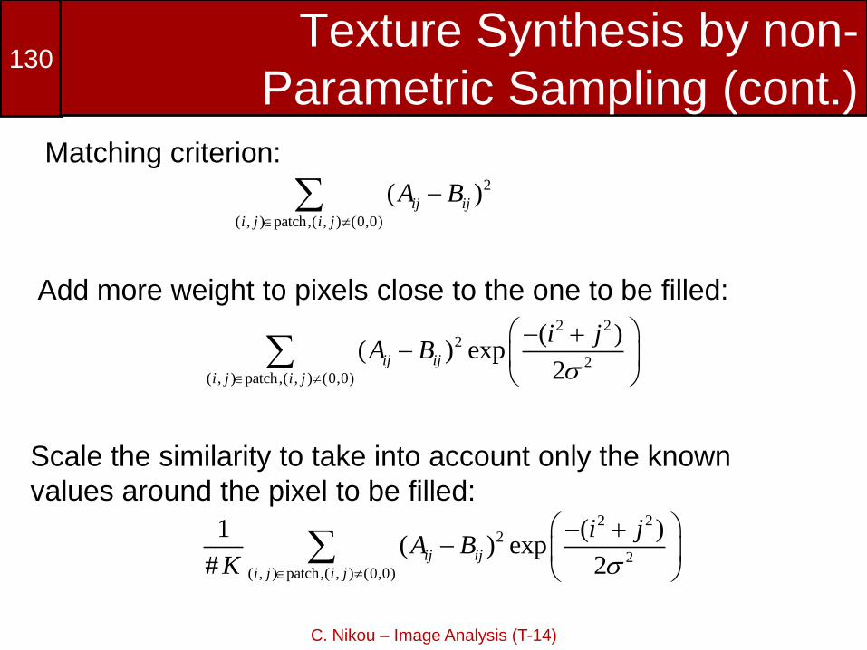
Matching criterion:2
( , ) patch,( , ) (0,0)
( )
ij ij
i j i j
A B
Add more weight to pixels close to the one to be filled:2 2
2
2( , ) patch,( , ) (0,0)
( )( ) exp
2
ij ij
i j i j
i jA B
Scale the similarity to take into account only the known
values around the pixel to be filled:2 2
2
2( , ) patch,( , ) (0,0)
1 ( )( ) exp
# 2
ij ij
i j i j
i jA B
K
131
C. Nikou – Image Analysis (T-14)
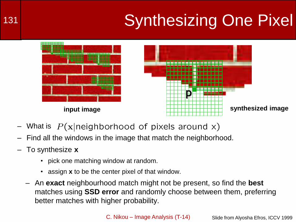
– What is ?
– Find all the windows in the image that match the neighborhood.
– To synthesize x
• pick one matching window at random.
• assign x to be the center pixel of that window.
– An exact neighbourhood match might not be present, so find the best
matches using SSD error and randomly choose between them, preferring
better matches with higher probability.
p
input image synthesized image
Slide from Alyosha Efros, ICCV 1999
Synthesizing One Pixel
132
C. Nikou – Image Analysis (T-14)
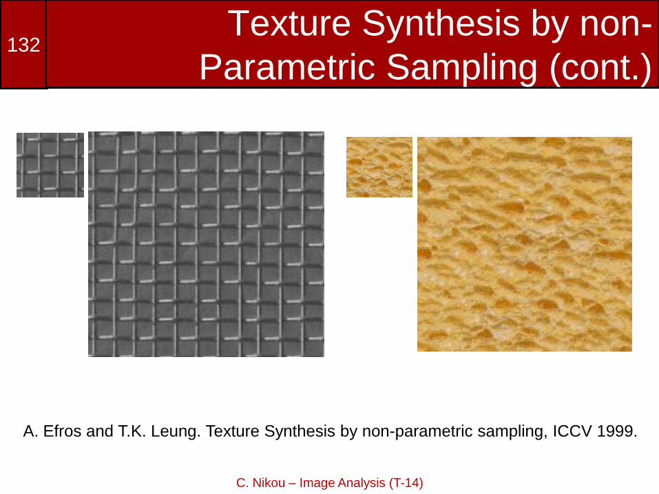
Texture Synthesis by non-
Parametric Sampling (cont.)
A. Efros and T.K. Leung. Texture Synthesis by non-parametric sampling, ICCV 1999.
133
C. Nikou – Image Analysis (T-14)
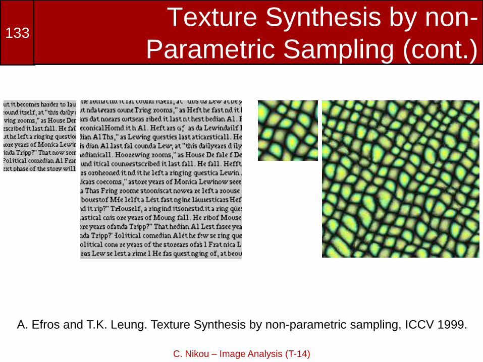
Texture Synthesis by non-
Parametric Sampling (cont.)
A. Efros and T.K. Leung. Texture Synthesis by non-parametric sampling, ICCV 1999.
134
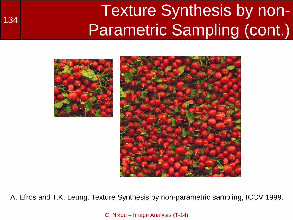
C. Nikou – Image Analysis (T-14)
Texture Synthesis by non-
Parametric Sampling (cont.)
A. Efros and T.K. Leung. Texture Synthesis by non-parametric sampling, ICCV 1999.
135
C. Nikou – Image Analysis (T-14)
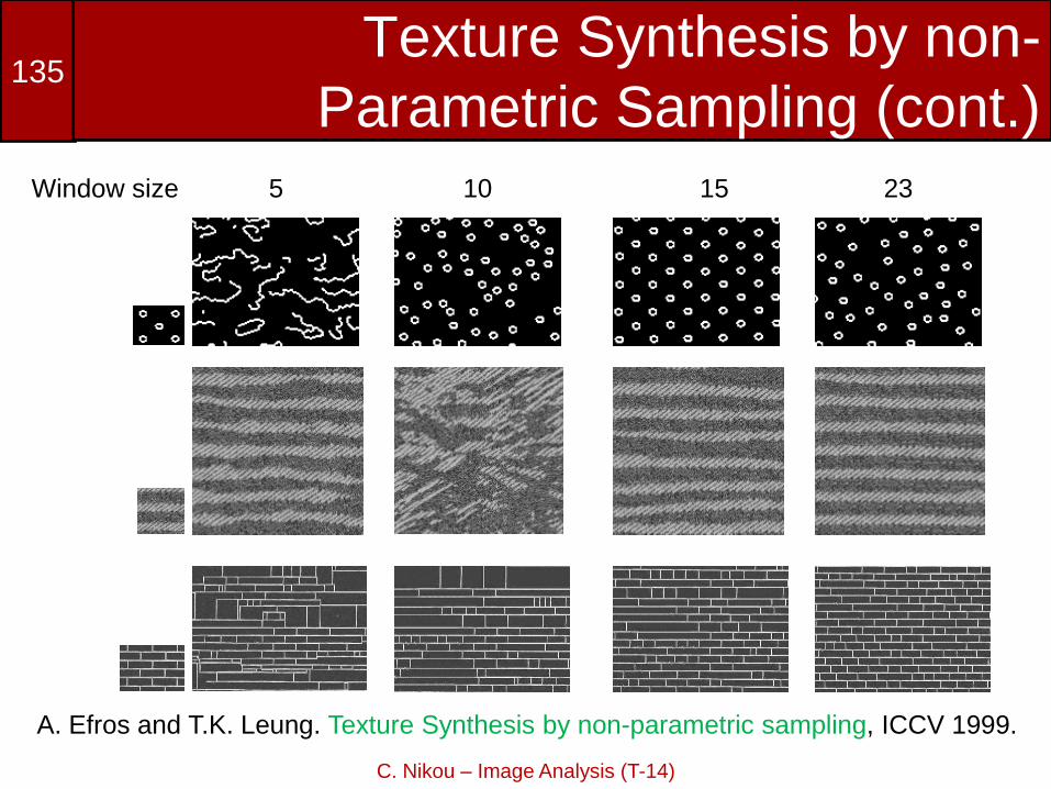
Texture Synthesis by non-
Parametric Sampling (cont.)
A. Efros and T.K. Leung. Texture Synthesis by non-parametric sampling, ICCV 1999.
5 10 15 23Window size
136
C. Nikou – Image Analysis (T-14)
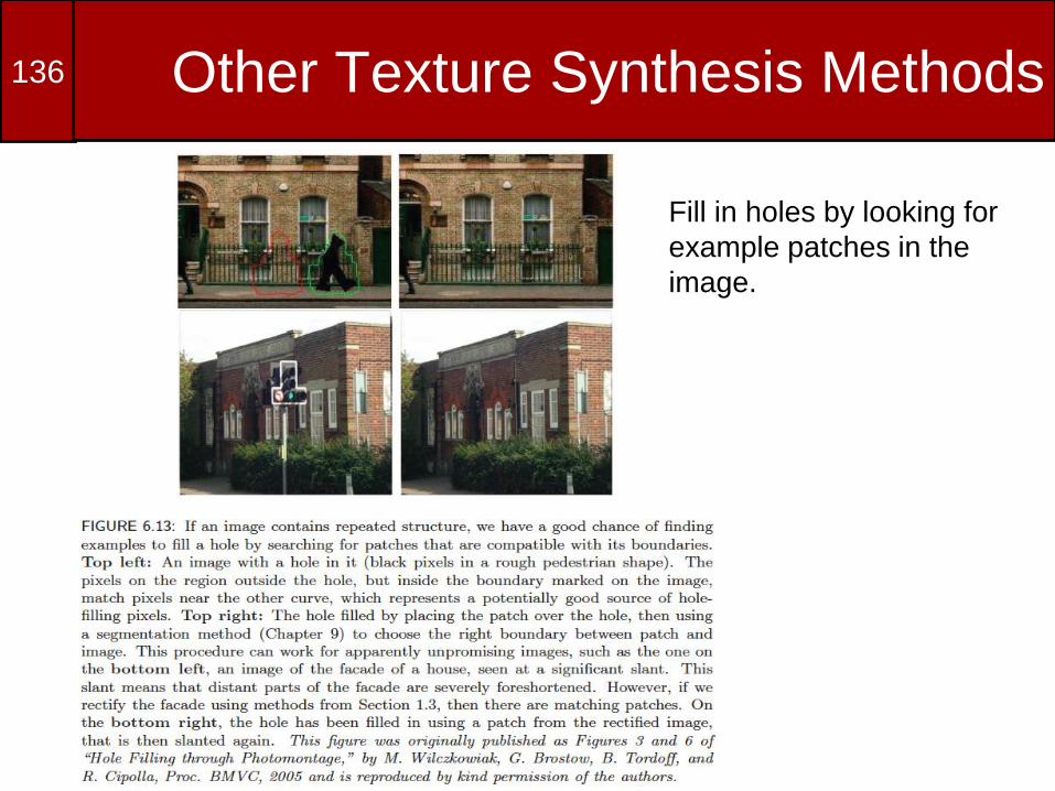
Other Texture Synthesis Methods
Fill in holes by looking for
example patches in the
image.
137
C. Nikou – Image Analysis (T-14)
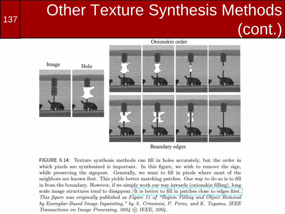
Other Texture Synthesis Methods
(cont.)
138
C. Nikou – Image Analysis (T-14)
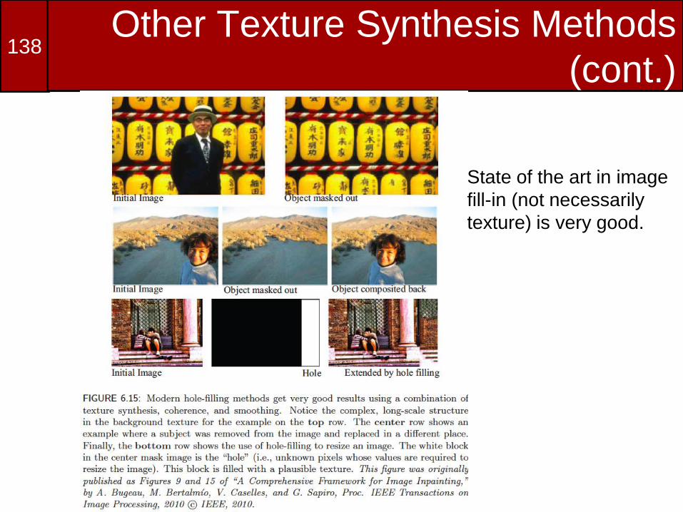
Other Texture Synthesis Methods
(cont.)
State of the art in image
fill-in (not necessarily
texture) is very good.