IM SYLLABUS (2015) PHYSICS IM 26 SYLLABUS - skolaphysics.skola.edu.mt/wp-content/downloads/syllabus/MATSEC/IM_26... · A course of study intended to prepare students for the Intermediate

1

PHYSICS IM 26 SYLLABUS

IM Syllabus (2015): Physics

IM SYLLABUS (2015)

2

Physics IM 26 (Available in September ) Syllabus 1 Paper (3hrs) Aims of the Intermediate Level Physics Curr iculum A course of study intended to prepare students for the Intermediate Level Matriculation Examination in Physics should: • promote an understanding of the nature and essence of physical principles; • foster implementation of the scientific approach in the analysis of real life situations; • encourage the development of problem solving techniques; • foster an appreciation and enjoyment of physics as a part of universal human culture; • encourage the development of practical skills; • provide an appreciation that physical laws are universal; • cultivate an appreciation of the influence of physics in everyday life; • encourage an understanding of technological applications of physics and its importance as a subject of

social, economic and industrial relevance. Examination The examination consists of ONE three-hour written paper having the following structure. Section A - 8 to 10 short compulsory questions, which in total carry 50% of the marks (90 minutes). Section B - 1 compulsory question on data analysis, which carries 14% of the marks (25 minutes). Section C - 4 longer structured questions to choose 2, each carrying 18% of the marks i.e. 36% allotted for the Section (65 minutes). It should be noted that while the students will not be tested in a formal practical examination, it is expected that they will have some opportunity to familiarise themselves with some basic experimental techniques and experiments illustrating the syllabus content during their studies. Questions may be set testing the students’ familiarity with the main experiments mentioned in the syllabus. Notes: • Scientific calculators may be used throughout the examination. Nevertheless, the use of graphical

and/or programmable calculators is prohibited. Disciplinary action will be taken against students making use of such calculators.

• Published by the MATSEC Unit is a Data and Formulae Booklet, which will be made available to the candidates during the examination.

Assessment Objectives • Knowledge with understanding (40%) • Applications of concepts and principles (35%) • Communication and presentation (10%) • Analysis of experimental data (15%)


3

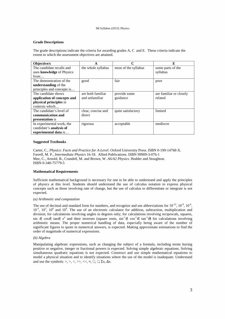
Grade Descr iptions The grade descriptions indicate the criteria for awarding grades A, C and E. These criteria indicate the extent to which the assessment objectives are attained. Objective/s A C E The candidate recalls and uses knowledge of Physics from…

the whole syllabus most of the syllabus some parts of the syllabus

The demonstration of the understanding of the principles and concepts is…

good fair poor

The candidate shows application of concepts and physical pr inciples in contexts which…

are both familiar and unfamiliar

provide some guidance

are familiar or closely related

The candidate’s level of communication and presentation is

clear, concise and direct

quite satisfactory limited

In experimental work, the candidate’s analysis of exper imental data is…

rigorous acceptable mediocre

Suggested Textbooks Carter, C., Physics: Facts and Practice for A-Level. Oxford University Press. ISBN 0-199-14768-X. Farrell, M. P., Intermediate Physics 16-18. Allied Publications. ISBN 99909-3-076-1 Mee, C., Arnold, B., Crundell, M. and Brown, W. AS/A2 Physics. Hodder and Stoughton. ISBN 0-340-75779-5 Mathematical Requirements Sufficient mathematical background is necessary for one to be able to understand and apply the principles of physics at this level. Students should understand the use of calculus notation to express physical concepts such as those involving rate of change, but the use of calculus to differentiate or integrate is not expected.

(a) Arithmetic and computation

The use of decimal and standard form for numbers, and recognize and use abbreviations for 10-12, 10-9, 10-6, 10-3, 103, 106 and 109. The use of an electronic calculator for addition, subtraction, multiplication and division; for calculations involving angles in degrees only; for calculations involving reciprocals, squares, sin θ, cosθ, tanθ, xn and their inverses (square roots, sin-1θ, cos-1θ, tan-1θ) for calculations involving arithmetic means. The proper numerical handling of data, especially being aware of the number of significant figures to quote in numerical answers, is expected. Making approximate estimations to find the order of magnitude of numerical expressions.

(b) Algebra

Manipulating algebraic expressions, such as changing the subject of a formula, including terms having positive or negative, integer or fractional powers is expected. Solving simple algebraic equations. Solving simultaneous quadratic equations is not expected. Construct and use simple mathematical equations to model a physical situation and to identify situations where the use of the model is inadequate. Understand and use the symbols: =, >, <, >>, <<, ≈, ∝, ∼, Σx, ∆x.


4

(c) Geometry and trigonometry

Calculate the areas of triangles, the circumference and areas of circles, and the surface areas and volumes of rectangular blocks, cylinders and spheres. Use Pythagoras’ theorem, similarity of triangles and the angle sum of a triangle and a quadrilateral. Use sines, cosines and tangents in physical problems.

(d) Graphs

Translate information between numerical, algebraic, written and graphical form. Select and plot two variables from experimental or other data, choosing suitable scales for graph plotting. Drawing a suitable best straight line through a set of data points on a graph. Understanding and using the standard equation of a straight-line graph y = mx + c, and rearranging an equation to linear form where appropriate. Determine the gradient and intercept of a linear graph. Sketch and recognize plots of common expressions like y = kx, y = kx2, y = k/x, y = k/x2, Interpret rate of change as the gradient of the tangent to a curve and its determination from a suitable graph. Understand the notation dx/dt as the gradient of the graph of x against t, and hence the rate of change of x with t. Understand and use the area between a curve and the relevant axis when this area has physical significance, and to be able to calculate it or measure it by estimation or by counting squares as appropriate. Syllabus

1. PHYSICAL QUANTITIES

1.1 Base quantities and units of the S.I . Base quantities:

Mass (kilogram, kg), length (metre, m), time (second, s), current (ampère, A), temperature interval (kelvin, K), amount of substance (mole).

Definitions of derived quantities may be given in terms of a word equation, e.g. Momentum = mass times velocity. The ability to obtain derived units in terms of base units will be examined. Definitions of the base units will not be examined.

Homogeneity of physical equations. Homogeneity (using base units of the S.I. system only and not dimensions) as a necessary but not sufficient condition for the correctness of physical equations. The use of base units or dimensions to derive physical relationships is not required.

1.2 Scalar and vector quantities:

The composition and resolution of vectors. Recognition of physical quantities as either vectors or scalars. Addition of two perpendicular vectors. Resolution of a vector into two perpendicular components.

2. MECHANICS

2.1 Rectilinear motion:

Displacement, speed, velocity and acceleration. Equations for uniformly accelerated motion. Displacement-time and velocity-time graphs.

Experimental measurement of velocity and the subsequent calculation of acceleration. Velocity = rate of change of displacement with time = slope of displacement-time graph = ∆s/∆t. Acceleration = rate of change of velocity with time = slope of velocity-time graph = ∆v/∆t. The ability to differentiate and integrate will not be examined.


5

Direct measurement of the acceleration of free fall.

Simple experiment.

Horizontally projected particle. Simple problems only.

2.2 Newton’s laws of motion:

Newton’s first law. Forces outside the nucleus may be either gravitational or electromagnetic. The use of free-body diagrams to represent forces acting on bodies. Velocity-time graph for a body fall ing in a viscous medium; terminal speed. Laws of friction are not included.

Linear momentum.

Newton’s second law. Force = ∆(mv)/∆t.

The newton The reasoning from the second law to the definition of the newton should be understood.

Newton’s third law. Students should be able to identify appropriate pairs of Newton third law forces.

Conservation of linear momentum in elastic and inelastic collisions.

Conservation of momentum for motion in one dimension only. Knowledge of experimental method is expected. Problems involving the solution of quadratic equations will not be set in the examination.

2.3 Energy:

Work. Work is defined as force multiplied by displacement in the direction of the force.

Potential energy. Energy stored in a stretched or compressed material is equal to area under force against extension or force against compression graph.

Gravitational potential energy close to the Earth’s surface.

The acceleration due to gravity, g, is assumed constant.

Kinetic energy. The derivation of kinetic energy = ½ mv2 is not required.

Law of conservation of energy.

2.4 Circular motion:

Centripetal acceleration and centripetal force. The necessity of an unbalanced force for circular motion of a particle moving with constant linear speed. Knowledge of a = v2/r is required but its derivation will not be examined. No reference to angular speed ω is expected.


6

3. THERMAL PHYSICS

3.1 Temperature and heat energy.

Thermal equilibrium and temperature. Temperature regarded as a property, which changes physical parameters such as length of a mercury column, the electromotive force of a thermocouple and the resistance of a wire.

Practical use of thermometers. Practical Celsius scale defined by θ = 100(Xt – Xo)/(X100 – Xo), where X could be the length of a liquid column, the electromotive force of a thermocouple, the resistance of a wire or the pressure of gas at constant volume. Conversion from Celsius to Kelvin scale using T(K) = θ(°C) + 273.15 K.

Heat defined as energy transfer due to a temperature difference.

3.2 Energy transfer :

Energy transfer by mechanical and electrical processes, or by heating.

Use of W = F ∆s; W = P ∆V; W = QV; Q = mc∆T; Q = mL.

Pressure-Volume diagrams Significance of the area under graph; restricted to isobaric and isochoric processes.

First law of thermodynamics. Meaning of ∆U, ∆Q and ∆W in ∆U = ∆Q + ∆W. The first law applied to a gas enclosed in a cylinder with a movable piston, to a filament lamp and the deformation of a metal wire.

3.3 Heating matter :

Measurement of specific heat capacity and specific latent heat by electrical methods.

Simple direct measurements emphasizing energy conversion. Identification of experimental errors. Calculation of heat losses is not included. Constant flow techniques are not expected.

4. MATERIALS

4.1 Solids:

Force against extension graphs for metals, rubber and glassy substances.

Hooke’s law, proportionality limit, elastic limit, yield point and breaking point are included. Elastic and plastic behaviour should be discussed. Knowledge of experimental work with metals and rubber is expected.

Stress, strain and Young’s modulus. Knowledge of an experiment to determine Young’s modulus of a metal in the form of a long wire is expected.


7

5. ELECTRICAL CURRENTS

5.1 Charge and cur rent:

Current as the rate of flow of charge. Current = slope of charge against time graph = dQ/dt.

Current model. Derivation of I = nAve. Distinction between conductors, insulators and semiconductors using this equation.

Electrical potential difference. Potential difference = work done/charge

Electromotive force of a cell. Definition of electromotive force.

The slide wire potentiometer is not expected.

5.2 Resistance:

Current-voltage curves for a wire at constant temperature, filament lamp and diode.

Knowledge of experimental investigations is expected.

Internal resistance of a cell and its measurement.

Practical importance of internal resistance in a car battery and extra high-tension supply. Slide wire methods are not required.

Resistors in series and in parallel. Use of LDR or thermistor to control voltage. Simple circuit problems. The Wheatstone bridge is not required.

The potential divider.

Energy and power in d.c. circuits. Energy = IVt = I2Rt = V2t/R. Power = IV = I2R = V2/R. The kilowatt-hour.

Use of ammeters, voltmeters and multimeters.

Knowledge of the internal structure of electrical meters and their conversion to different ranges are not required.

6. FIELDS

6.1 Gravitational fields:

Newton’s law of gravitation.

Gravitational field strength, g. Variation of g with height above Earth’s surface. Questions on gravitational potential will not be set.

Representation of radial gravitational field lines.

Motion of satellites in circular orbits. Use of mv2/r = GMm/r2 and T = 2πr/v.


8

6.2 Electrostatic fields:

Simple electrostatic phenomena. Charging conductors by induction. Point charges in vacuum.

Inverse square law in electrostatics. Experimental demonstration is not required.

Use of lines of force to describe electric fields qualitatively.

Electric field strength defined as, E = F/q. The electric force F on a charge q in an electric field E is given by F = Eq.

Work done when charge moves in a uniform electric field.

Use of V= Ed.

Acceleration of charged particles moving along the field lines of a uniform electric field.

QV = ∆( ½ mv2). The electron-volt.

Deflection of charged particles in uniform electric fields.

Qualitative description only.

6.3 Capacitors:

Factors affecting the capacitance of a parallel plate capacitor.

Relative permittivity. Q = CV; εr = C/Co; C = εoεrA/d. No experimental determination of the listed parameters is expected.

Growth and decay of charge stored in a capacitor in series with a resistor. Time constant.

Exponential form of a graph to be understood and related to the decay of radioactivity. Use of graph to determine RC, as time taken for the charge and voltage to drop to 1/e (approximately 37%) of its initial value. Equations for growth and decay of charge are not required.

6.4 Magnetic fields:

Magnetic effect of a steady current. B-field patterns near a straight conductor and solenoid.

Magnetic flux density. The tesla. B defined from F = BIl. Vector nature of B.

Force on a charged particle moving through a magnetic field.

Derivation of F = BQv from F = BIl and I = nAve. (BQv = mv2/r)

6.5 Electromagnetic induction:

Magnetic flux. Flux linkage. Experimental demonstration that cutting flux or change in flux linkage induces an emf.

Faraday’s and Lenz’s laws of E = −Ndφ/dt. Lenz’s law and energy conservation.


9

electromagnetic induction. The derivation of E = Blv is not required.

The simple generator. Qualitative study of electromotive force produced when a rectangular coil rotates in a uniform magnetic field as an introduction to sinusoidal alternating current.

Peak and root mean square values and their relationship for sinusoidal currents and voltages.

Knowledge of Irms = Io/√2 and Vrms = Vo/√2. Derivations of these equations are not expected.

Use of the oscilloscope to measure voltage and time intervals.

Knowledge of the internal structure of the oscilloscope is not required.

7. VIBRATIONS AND WAVES

7.1 Simple harmonic motion:

Definition of simple harmonic motion. a = –k x; k

T π2= where k is a positive

constant.

Displacement-time, velocity-time and acceleration-time graphs for a body in simple harmonic motion.

Graph obtained from experiment.

Energy as a function of displacement in simple harmonic motion.

Qualitative description of energy conversion in simple harmonic motion.

Natural and forced vibrations.

Mechanical resonance. Including vibrating strings.

7.2 Mechanical waves:

Longitudinal and transverse progressive waves.

Emphasis on energy transmissions by waves.

Amplitude, speed, wave length, frequency and phase interpreted graphically.

Displacement-position and displacement-time graphs. Phase difference should be expressed as a fraction of a cycle, wavelength or periodic time. No reference to phase in radians is expected.

7.3 Superposition of waves:

The superposition principle applied to the formation of stationary waves in a string.

Displacement-position graphs used to explain formation of nodes and antinodes.

Contrast between progressive and stationary waves.

Experimental treatment of diffraction of water waves at a single slit.

Effect of slit and wavelength on pattern relative size.

Interference of water waves in the two-slit Explanation of the formation of the interference


10

experiment pattern in terms of phase difference between the two wave trains. Effect on pattern of changes in point source separation and frequency.

Young’s double slit experiment. Looking at a slit source through two close, narrow slits to demonstrate the wavelike nature of light. Use of the formula λ = yd/D is required but not its proof.

7.4 Optics:

Laws of reflection and refraction. Refractive index.

Reflection and refraction at plane interfaces only.

Total internal reflection and critical angle.

Dispersion. Dispersion of l ight by a prism. Continuous spectrum from white light source.

Refraction of light by a thin converging lens.

Use of the lens equation and equation for magnification in any one sign convention. Experimental determination of the focal length by using these equations.

8. PHYSICS OF NUCLEI AND ATOMS

8.1 Energy levels and spectra:

Energy levels of isolated atom. Students should know that the possible energy states of an atom are discrete.

The emission of light by atoms. Qualitative explanation of emission line spectra. Use of E1 − E2 = hf. Line spectrum from a discharge tube.

8.2 Atomic structure:

Evidence for a nuclear atom. Alpha scattering experiment.

Emphasis on the results of the experiment and their qualitative interpretation.

Properties of alpha, beta (−) and gamma radiation and corresponding disintegration processes.

Knowledge of qualitative experiments on absorption of radiation from sealed sources is expected.

Health hazards and protection.

Radioactivity as a random process. Background radiation and its sources.

Radioactivity decay. Use of A = λN. N = No e−λt is not required.

Concept of half-life. Use of T½ = 0.693/λ.


11

Nuclear reactions. The atomic mass unit, u. Equivalence of mass and energy. Use of E = mc2. Students should be familiar with the terms fission and fusion as examples of nuclear reactions. Concept of binding energy is not required.


Documents

IM SYLLABUS (2015) PHYSICS IM 26 SYLLABUS - skolaphysics.skola.edu.mt/wp-content/downloads/syllabus/MATSEC/IM_26... · A course of study intended to prepare students for the Intermediate