Embed Size (px)
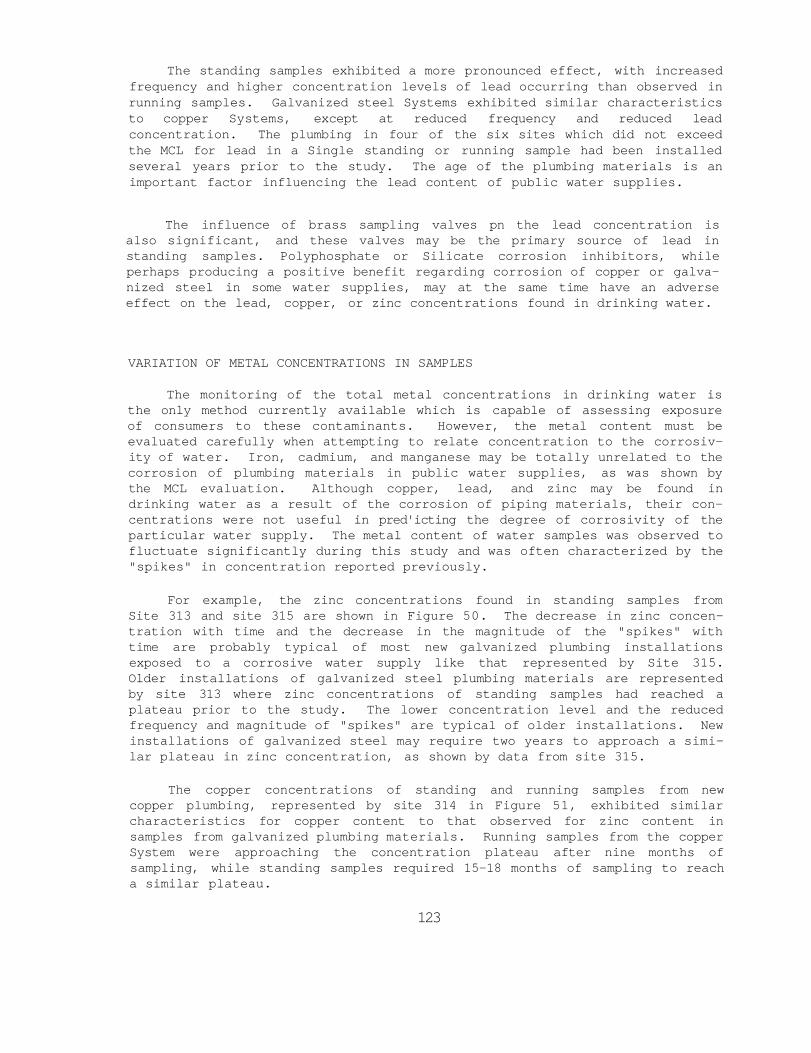
Citation preview
Prepared for the Water Engineering Research Laboratory
Office of Research and Development US Environmental Protection Agency
Champaign Illinois March 1987
RELATIONSHIPS BETWEEN WATER QUALITY
AND CORROSION OF PLUMBING MATERIALS IN BUILDINGS
VOLUME I GALVANIZED STEEL AND COPPER PLUMBING SYSTEMS
by
Chester H Neffand Michael R Schock Illinois State Water Survey
and
John I Marden University of Illinois
SWS Contract Report 416-I
Illinois State Water Survey Division AQUATIC CHEMISTRY SECTION
AT THE UNIVERSITY OF ILLINOIS
RELATIONSHIPS BETWEEN WATER QUALITY AND CORROSION OF PLUMBING MATERIALS IN BUILDINGS
VOLUME I GALVANIZED STEEL AND COPPER PLUMBING SYSTEMS
by
Chester H Neff and Michael R Schock Illinois Department of Energy and Natural Resources
Champaign Illinois 61820 and
John I Marden University of Illinois Urbana Illinois 61801
Grant No CR808566-02
Project Officer
Marvin C Gardeis Drinking Water Research Division
Water Engineering Research Laboratory Cincinnati Ohio 45268
WATER ENGINEERING RESEARCH LABORATORY OFFICE OF RESEARCH AND DEVELOPMENT US ENVIRONMENTAL PROTECTION AGENCY
CINCINNATI OHIO 45268
DISCLAIMER
Although the Information described in this article has been funded wholly or in part by the United States Environmental Protection Agency through assistance agreement number CR808566-02 to the Illinois State Water Survey Department of Energy and Natural Resources and the Board of Trustees of the University of Illinois it has not been subjected to the Agencys required peer and administrative review and therefore does not necessarily reflect the views of the Agency and no official endorsement should be inferred
ii
FOREWORD
The US Environmental Protection Agency is charged by Congress with protecting the Nations land air and water Systems Under a mandate of national environmental laws the agency strives to formulate and implement actions leading to a compatible balance between human activities and the ability of natural systems to support and nurture life The Clean Water Act the Safe Drinking Water Act and the Toxic Substances Control Act are three of the major congressional laws that provide the framework for restoring and maintaining the integrity of our Nations water for pre-serving and enhancing the water we drink and for protecting the environment from toxic substances These laws direct the EPA to perform research to define our environmental problems measure the impacts and search for solutions
The Water Engineering Research Laboratory is that component of EPAs Research and Development program concerned with preventing treating and managing municipal and industrial wastewater discharges establishing prac-tices to control and remove contaminants from drinking water and to prevent its deterioration during storage and distribution and assessing the nature and controllability of releases of toxic substances to the air water and land from manufacturing processes and subsequent product uses This publica-tion is one of the producta of that research and provides a vital communica-tion link between the researcher and the user community
Galvanized steel and copper plumbing materials have been used extensively in this country to distribute drinking water in buildings Corrosion of these materials within the distribution system may cause the drinking water to become contaminated by lead zinc and copper corrosion products This publication presents the findings of a corrosion study of galvanized steel and copper materials exposed to public water supplies in Illinois The relationships between water quality corrosion rates and metal concentrations are reported
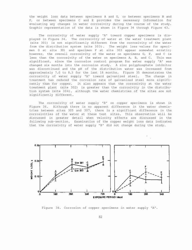
Francis T Mayo Director Water Engineering Research Laboratory
iii
ABSTRACT
A 3-year corrosion study was conducted on galvanized steel and copper piping materials installed in six public water supplies in Illinois The water supplies were selected to represent the influence of water source treatment processes corrosion control programs and water quality on the corrosivity of water A comprehensive water sampling program was imple-mented to quantify the total metal concentrations found in both standing and running water samples The major inorganic constituents in the water were determined to evaluate their contributions to the corrosivity of each water supply to copper or galvanized steel plumbing materials
Corrosion rates were measured by a weight loss method using the ASTM (D2688 Method C) corrosion tester Nineteen corrosion test sites were inshystalled to investigate the effects of time and changes in water quality on the corrosivity Corrosion data metal concentrations and water quality were incorporated into a data base from which multiple linear regression modeis were tested for significant data correlations
Several significant findings were observed- Most significant was the observation that chrome-plated brass faucets were making a large contribu-tion to the lead zinc and copper concentrations found in drinking water The experiments showed conclusively that brass sampling valves can be a considerable source of readily leachable lead and zinc when lead solder lead pipes and galvanized pipes are not present Metal concentrations in water were significantly reduced with increased age of the plumbing instal-lations Extremely high metal concentrations were observed under stagnant water conditions in new plumbing installations whereas reduced concentrashytions were observed in both running and standing water from older piping and fittings
The lead zinc copper iron and manganese concentrations exceeded the MCL in 106 to 256$ of the standing samples and in 22 to 160 of the running samples collected during the study Cadmium did not exceed the MCL in any sample The metal concentrations generally decreased to equilibrium values within 6 months at most sites but the zinc and copper concentrations increased during the last 12 months to concentrations much above the MCL in the most aggressive water supply
The statistical association analysis was unsuccessful because of the exceedingly large number of variables encountered under the field conditions of the study All six public water supplies experienced unanticipated upsets in water quality during the study The simulated corrosion test loops were effectively used to monitor the corrosivity of the water with improved control of the running and standing periods of sampling
iv
This report was submitted in fulfillment of Grant No CR808566010 by the Illinois Department of Energy and Natural Resources and the University of Illinois under the sponsorship of the US Environmental Protection Agency This report Covers the period from April 13 1981 to October 12 1984 and work was completed as of April 12 1985
v
CONTENTS
Foreword iii Abstract iv Figures x Tables xii Acknowledgments xiv
Volume I
1 Introduction 1 Scope and Objectives 1 Background 1 Project Design and Constraints 2 References 4
2 Conclusions 6 Method of Corrosion Measurement 6 Variability of Water Quality in Public Supplies 7 Effect of Water Quality on Corrosion Rates 7 Effects of Corrosion on Trace Metal Concentrations 8 Statistical Association of Water Quality Variables and
Corrosion Rates 9 Contribution of Trace Metals by Sampling Valves 10 Additional Laboratory Studies 11 Reference 11
3 Recommendations 12 References 15
4 Treatment Processes and Quality of Selected Water Supplies 16 Criteria Employed for Selecting Water Supplies 16 Water Supply A Carbondale IL 17 Water Supply B Champaign-Urbana IL 19 Water Supply C Dwight Correctional Center 20 Water Supply D Dwight IL 22 Water Supply E Wm Fox Developmental Center 24 Water Supply F Springfield IL 25 References 26
5 Corrosion Testing Program and Procedures 27 ASTM D2688 Corrosion Testers 27 Simulated Corrosion Test Loop Design 27 Corrosion Test Site Installations 30
Sites 301 and 302 30 Sites 303 and 304 32 Sites 305 and 306 33 Site 307 33 Sites 308 and 309 34
vii
CONTENTS (continued)
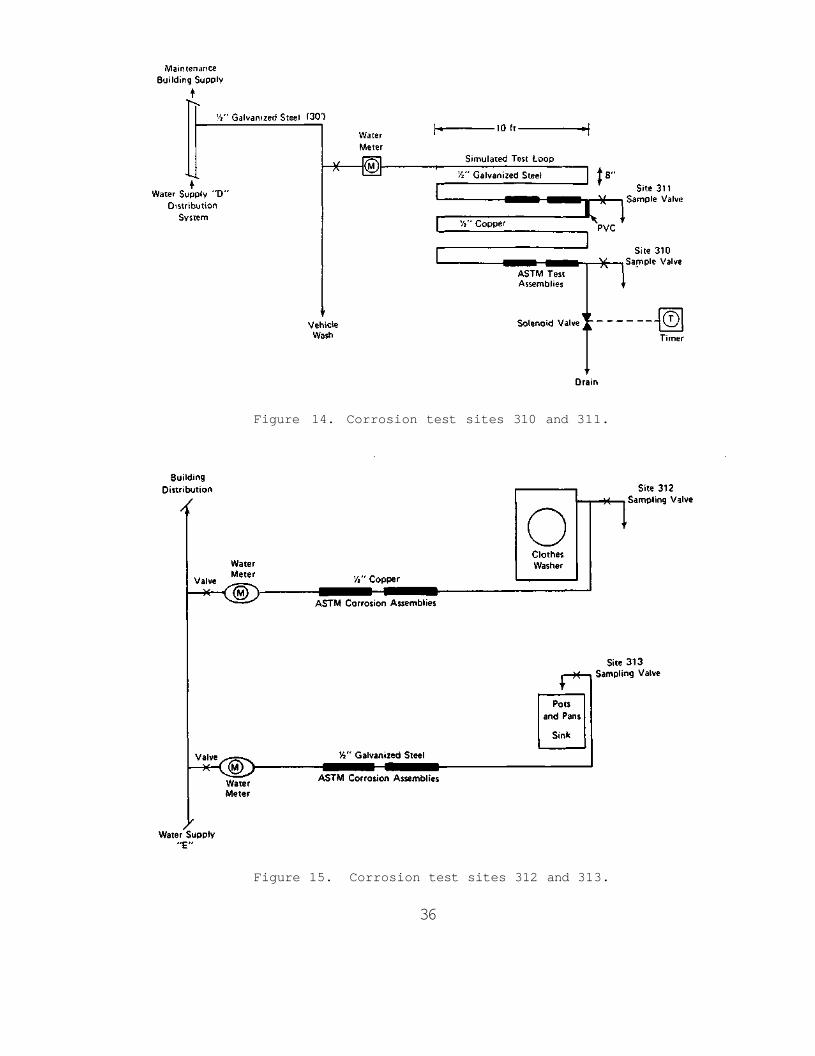
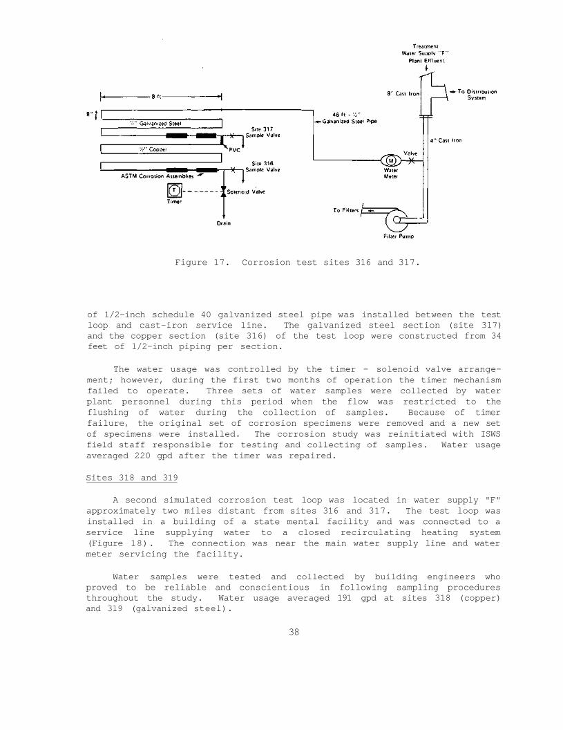
Sites 310 and 311 35 Sites 312 and 313 35 Sites 314 and 315 37 Sites 316 and 317 37 Sites 318 and 319 38
References 39 6 Field Methods for Collecting Handling and
Testing of Samples 40 Sample Collection Procedures 40 Sample Preservation and Handling Procedures 41 Field Test Methods 41
Chlorine Residuais 42 pH 42 Dissolved Oxygen 42 Temperature 42
References 43 7 Laboratory Analytical Methods 44
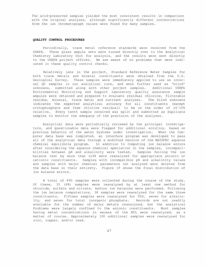
Trace Metal and Major Cation Determinations 44 Major Anion Determinations 44 Miscellaneous Analyses 46 Quality Control Procedures 47 Study of the Reversion of Polyphosphate to
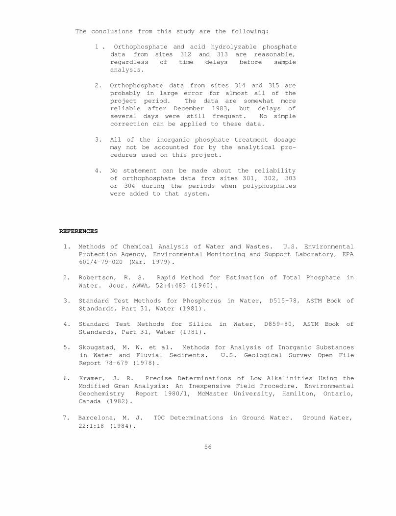
Orthophosphate 48 References 56
8 Laboratory Corrosion Investigations 58 Differentiation of Dissolved and Particulate
Products 58 Field Investigations of Contamination from
Sampling Valves 62 Laboratory Study of Trace Metal Leaching from
Sampling Taps 66 Comparison of Faucet Contamination Data to
Other Studies 67 X-Ray Diffraction Analysis of Deposits Found in
Corrosion Specimens 72 References 74
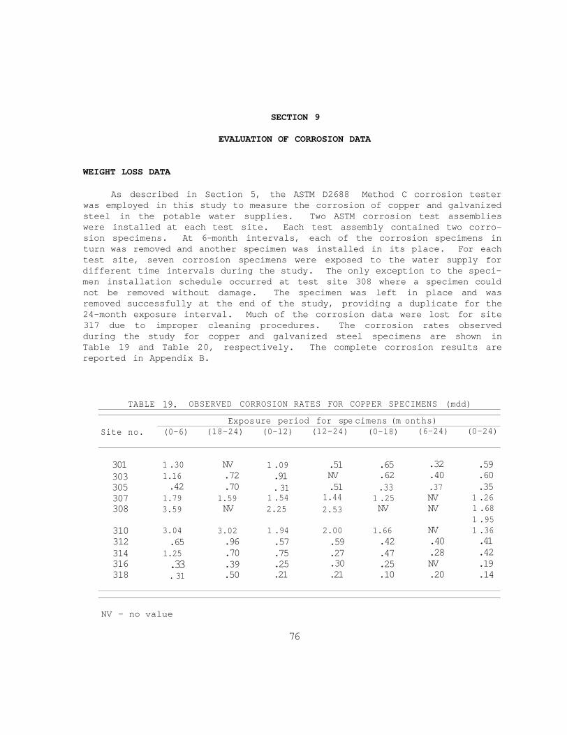
9 Evaluation of Corrosion Data 76 Weight Loss Data 76 Graphic Evaluation of the Corrosivity of the
Water Supplies 78 Data Evaluation by the Planned Interval
Test Method 81 Water Velocity Effects on Copper 88 Corrosion of Plumbing Materials during Long-Term
Curtailment of Water Usage 90 References 92
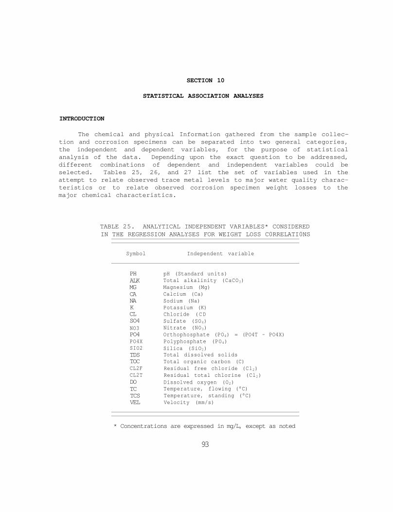
10 Statistical Association Analyses 93 Introduction 93
viii
CONTENTS (concluded)
Metals Estimated by Water Quality Variables within and between Sites 95
Estimation of Weight Loss from Water Quality Statistical Background 103
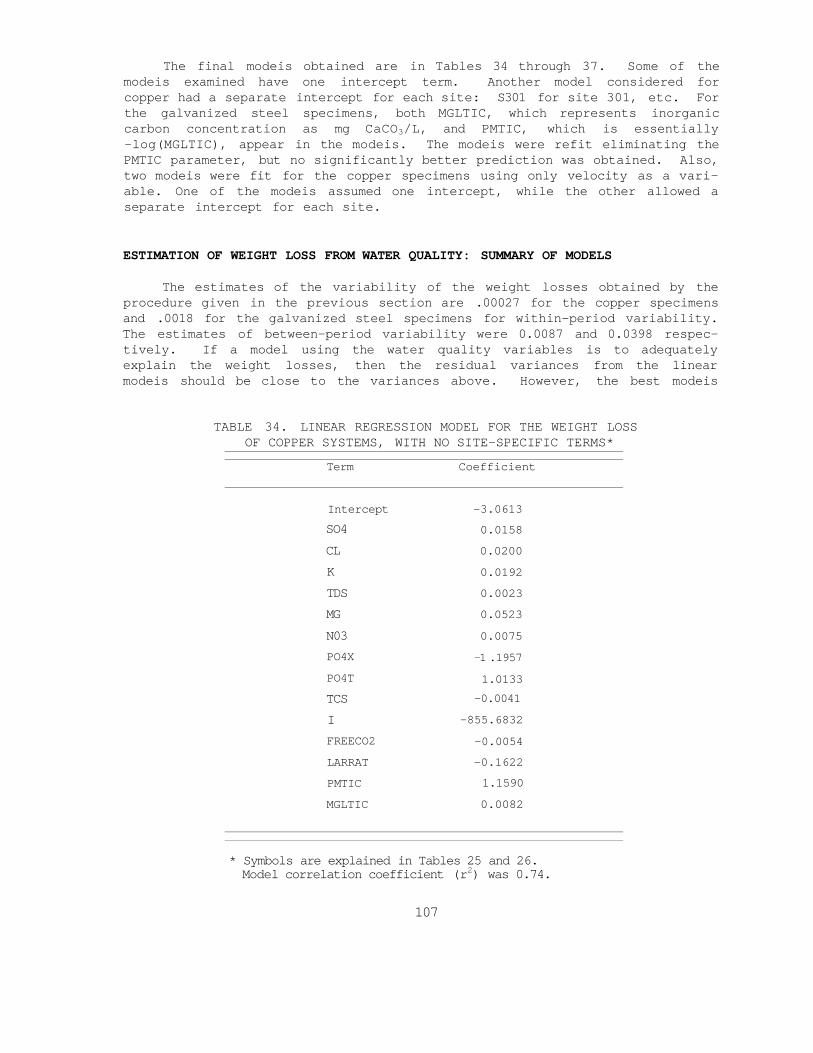
Estimation of Weight Loss from Water Quality Summary of Models 107
Conclusions and Recommendations 110 References 111
11 Significance of Metal Concentrations Observed in Public Water Supplies 112
Introduction 112 Samples Exceeding MCL Standards 112
Manganese 113 Iron 114 Zinc 117 Copper 119 Lead 121
Variation of Metal Concentrations in Samples 123 References 131
12 Project Summary 132 References 133
Volume II
Appendices A Analytical Data 1 B Corrosion Data 79 C Photos of Selected Pipe Specimens and Fittings 87 D Information for Collecting Water Samples
and Conducting Corrosion Tests 93
ix
FIGURES
Number Page
1 Water supply A treatment system 19 2 Water supply B treatment system 20 3 Water supply C treatment system 21 4 Water supply D treatment system 23 5 Water supply E treatment system 25 6 Water supply F treatment system 26 7 Cross section of specimen spacer sleeve
and union of assembled corrosion tester 28 8 Simulated corrosion test loop 29 9 Corrosion test sites 301 and 302 31
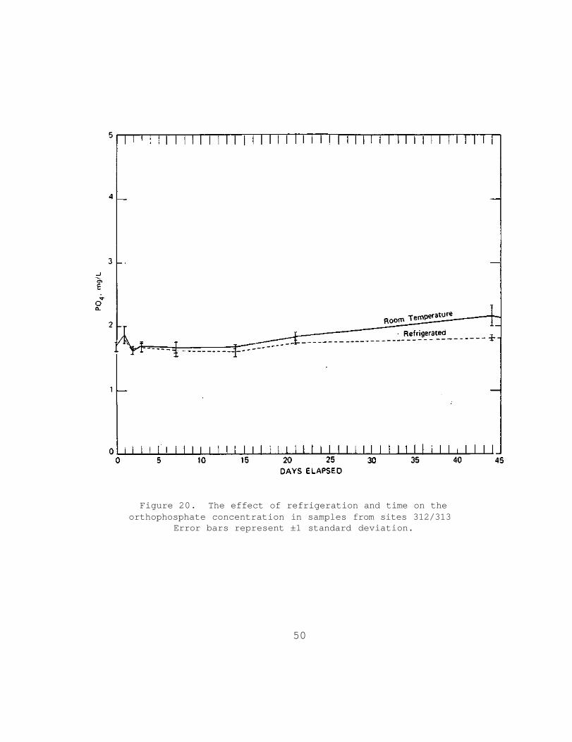
10 Corrosion test sites 303 and 304 32 11 Corrosion test sites 305 and 306 33 12 Corrosion test site 307 34 13 Corrosion test sites 308 and 309 35 14 Corrosion test sites 310 and 311 36 15 Corrosion test sites 312 and 313 36 16 Corrosion test sites 314 and 315 37 17 Corrosion test sites 316 and 317 38 18 Corrosion test sites 318 and 319 39 19 Distribution frequency of ion balance errors 48 20 The effect of refrigeration and time on the
orthophosphate concentration in samples from sites 312313 50
21 The effect of refrigeration and time on the acid hydrolyzable phosphate concentration in samples from sites 312313 51
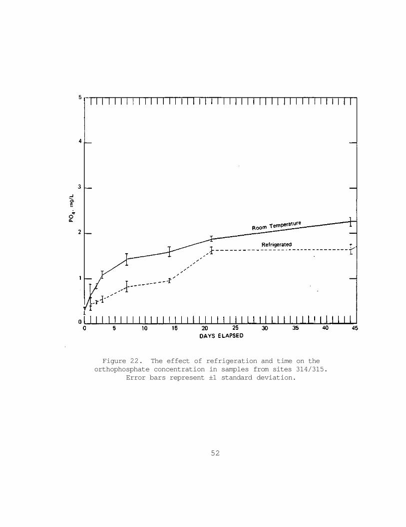
22 The effect of refrigeration and time on the orthophosphate concentration in samples from Sites 314315 52
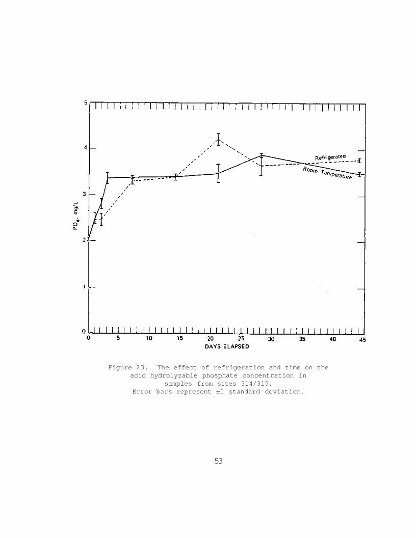
23 The effect of refrigeration and time on the acid hydrolyzable phosphate concentration in samples from sites 314315 53
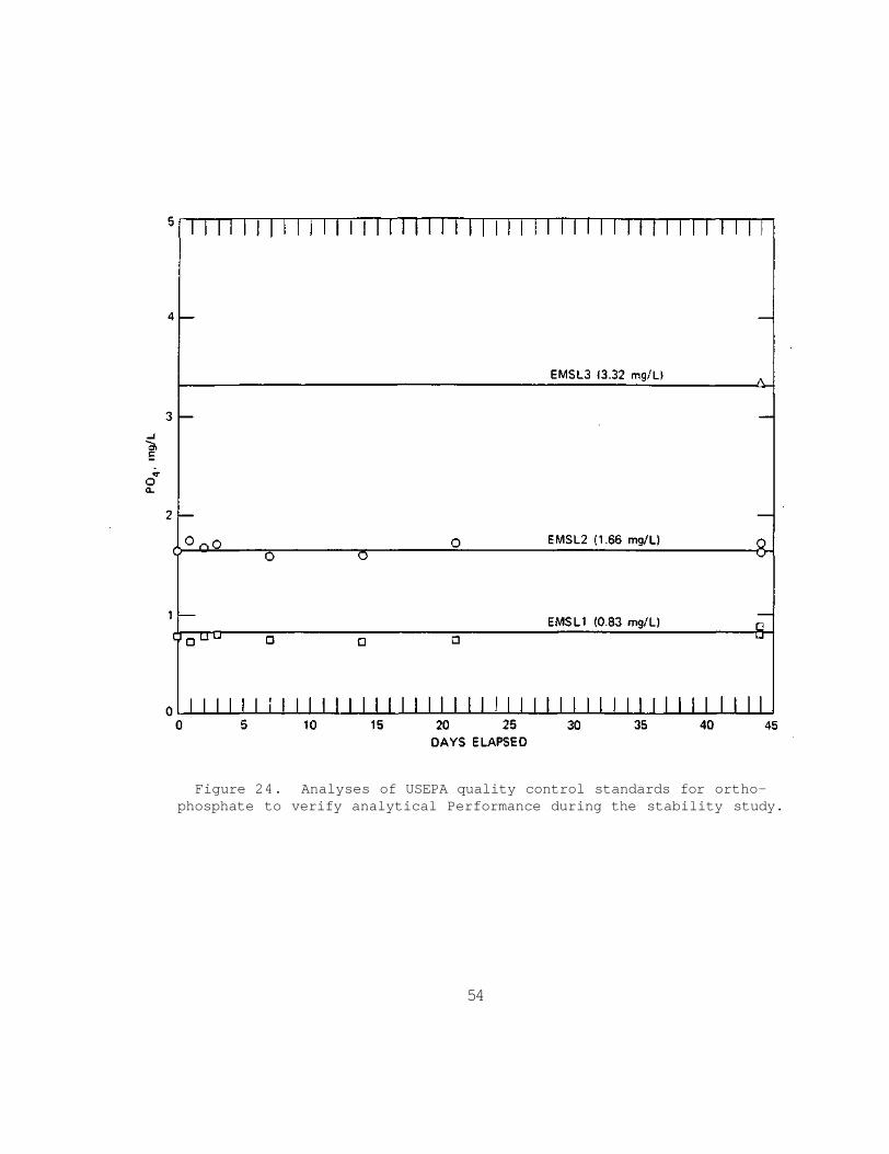
24 Analyses of USEPA quality control standards for orthophosphate to verify analytical Performance during the stability study 54
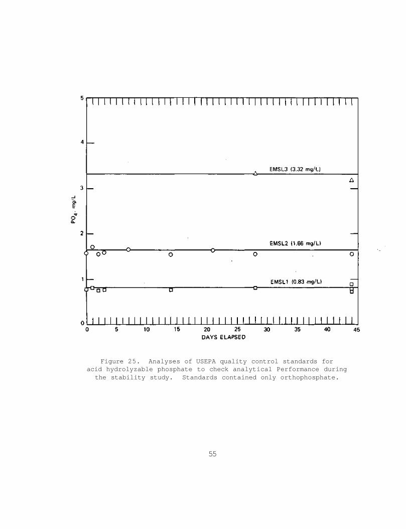
25 Analyses of USEPA quality control standards for acid hydrolyzable phosphate to check analytical Performance during the stability study 55
26 Results of 24-hour leaching study of lead from new chrome-plated sampling taps 67
x
FIGURES (concluded)
Number Page
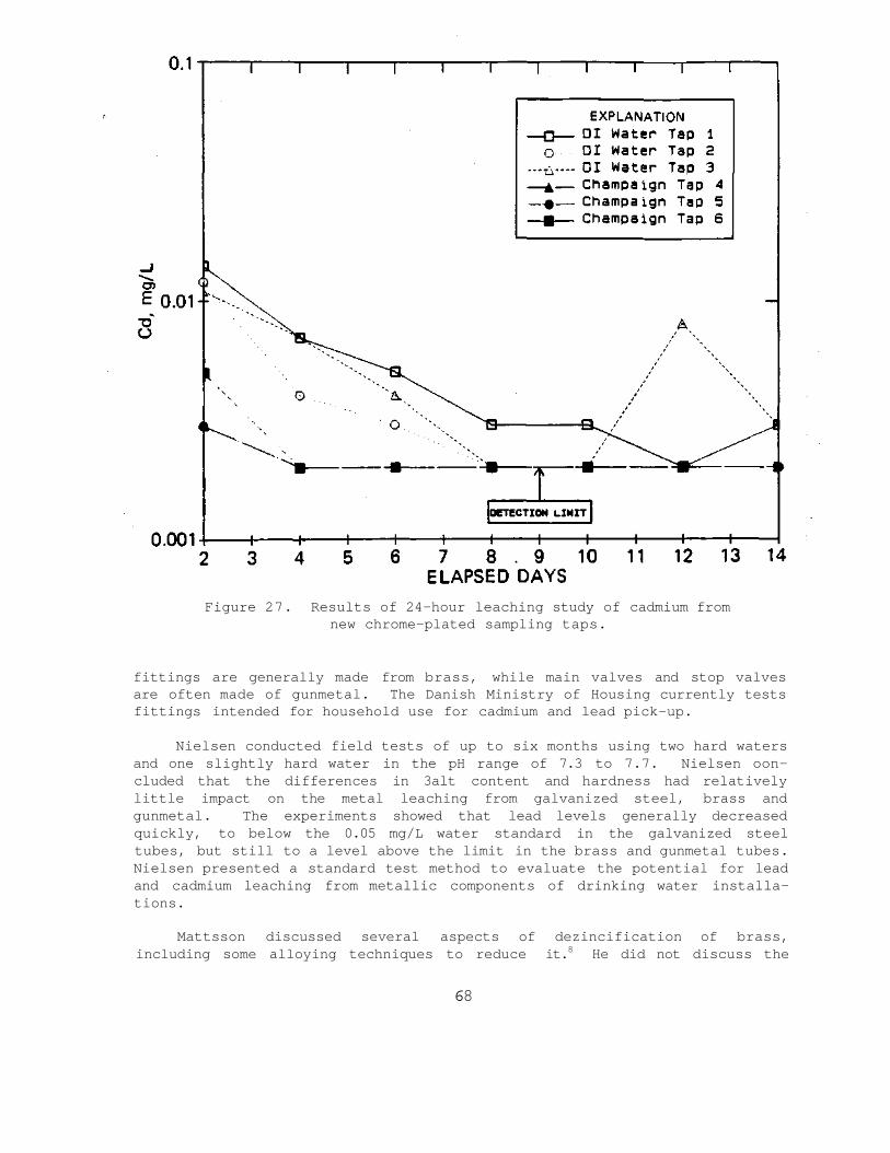
27 Results of 24-hour leaching study of cadmium from new chrome-plated sampling taps 68
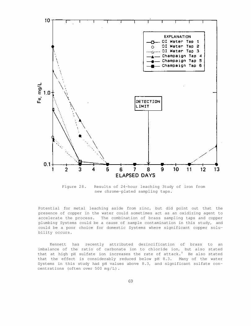
28 Results of 24-hour leaching study of iron from new chrome-plated sampling taps 69
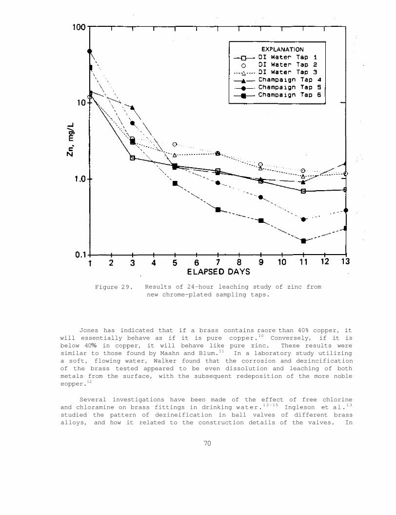
29 Results of 24-hour leaching study of zinc from new chrome-plated sampling taps 70
30 Results of 24-hour leaching study of copper from new chrome-plated sampling taps 71
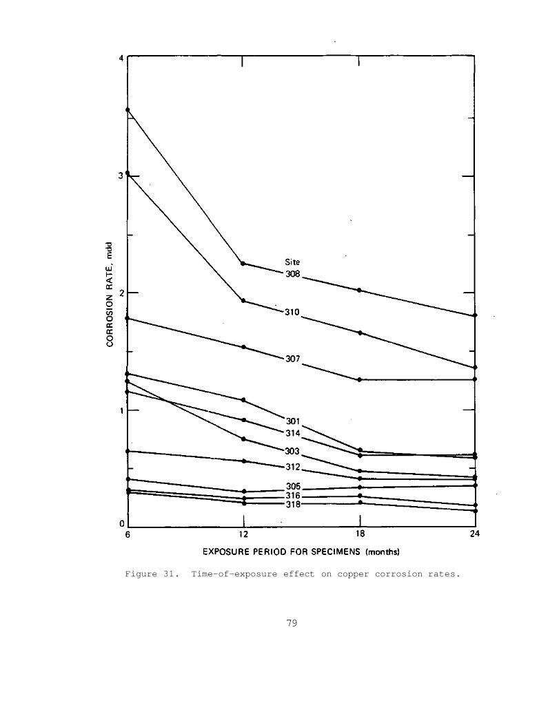
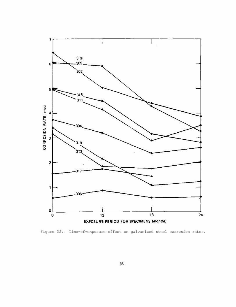
31 Time-of-exposure effect on copper corrosion rates 79 32 Time-of-exposure effect on galvanized steel corrosion
rates 80 33 Planned intervals of exposure for corrosion specimens 81 34 Corrosion of copper specimens in water supply A 82 35 Corrosion of galvanized steel specimens in water
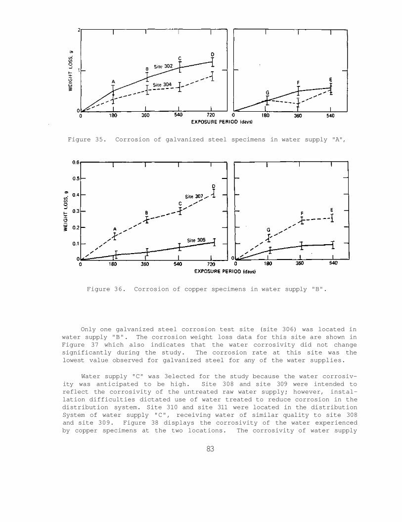
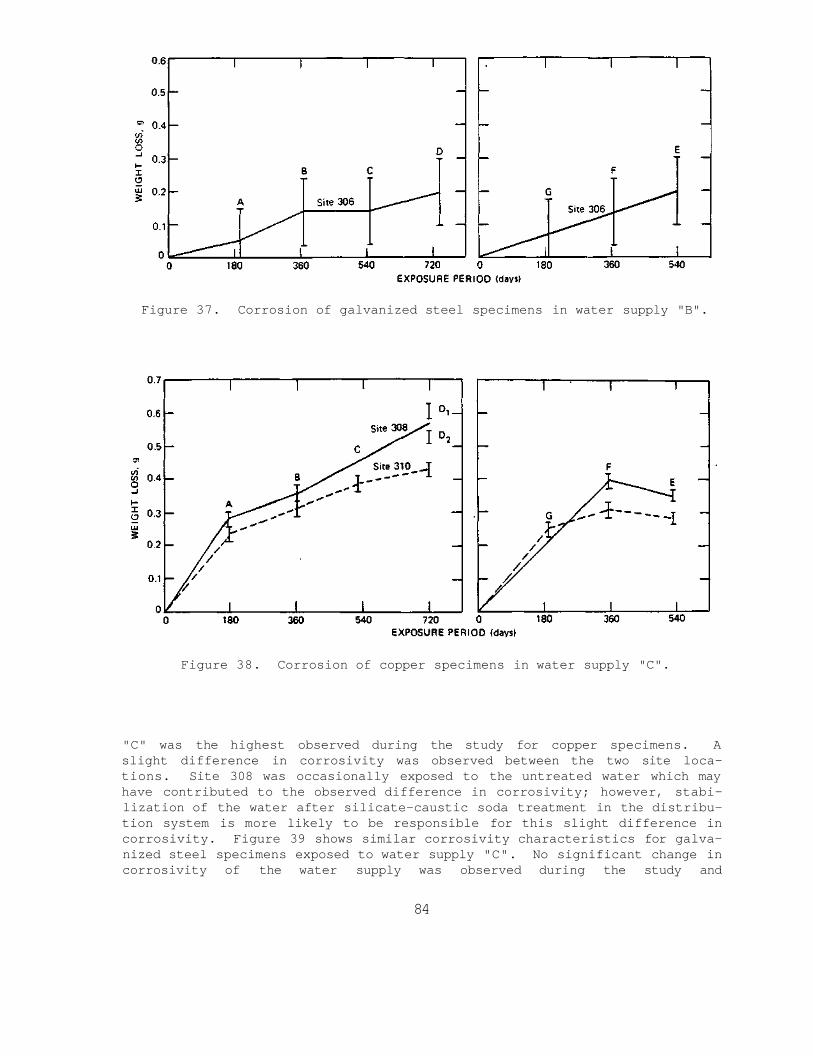
supply A 83 36 Corrosion of copper specimens in water supply B 83 37 Corrosion of galvanized steel specimens in water
supply B 84 38 Corrosion of copper specimens in water supply C 84 39 Corrosion of galvanized steel specimens in water
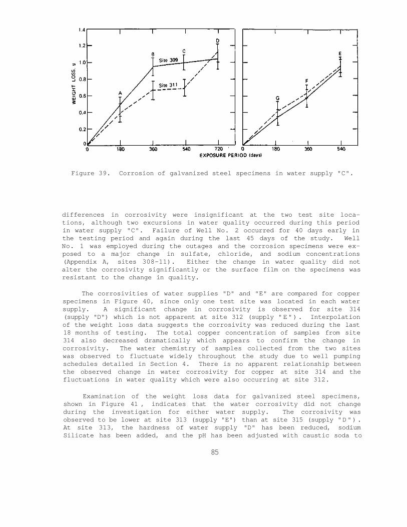
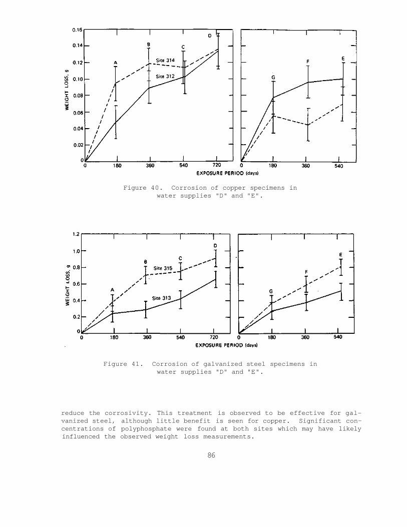
supply C 85 40 Corrosion of copper specimens in water supplies
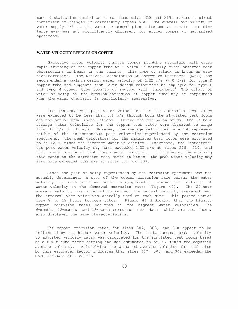
D and E 86 41 Corrosion of galvanized steel specimens in water
supplies D and E 86 42 Corrosion of copper specimens in water supply F 87 43 Corrosion of galvanized steel specimens in water
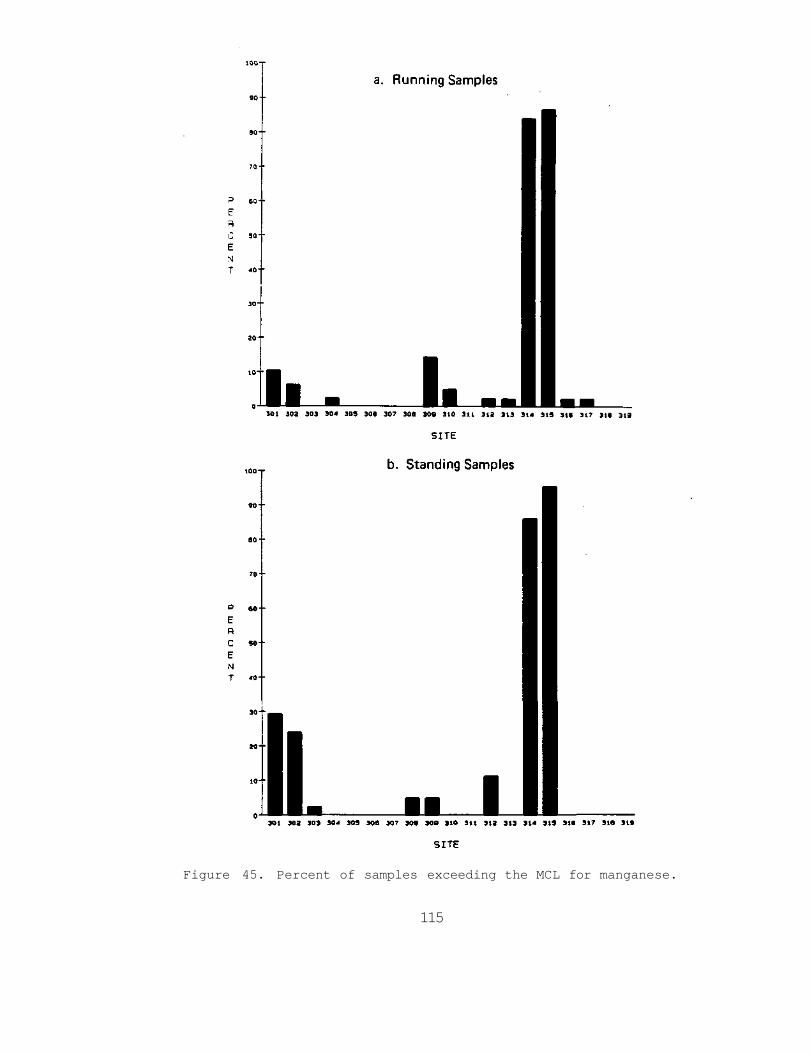
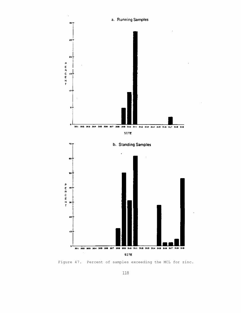
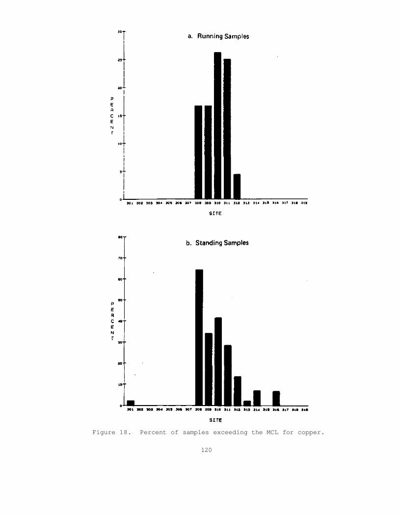
supply F 87 44 Effect of water velocity on corrosion rate of copper 89 45 Percent of samples exceeding the MCL for manganese 115 46 Percent of samples exceeding the MCL for iron 116 47 Percent of samples exceeding the MCL for zinc 118 48 Percent of samples exceeding the MCL for copper 120 49 Percent of samples exceeding the MCL for lead 122 50 Zinc concentrations of standing samples from sites
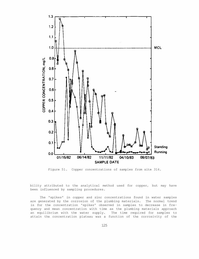
313 and 315 124 51 Copper concentrations of samples from site 314 125 52 Copper concentrations of samples from site 307 126 53 Copper concentrations of samples from site 310
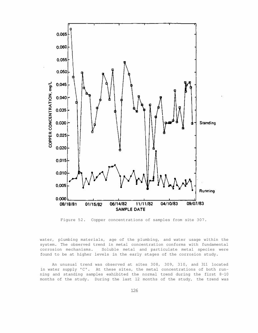
copper system 128 54 Zinc concentrations of samples from site 311
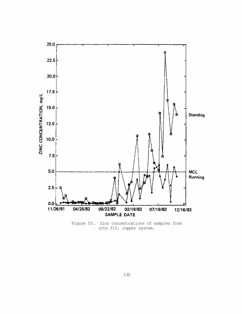
galvanized steel system 129 55 Zinc concentrations of samples from site 310
copper system 130
xi
TABLES
Number Page
1 Laboratory Analytical Load 4 2 Criteria Employed for Selecting Water Supplies 17 3 Range of Water Quality Parameters Tor Selected Public
Water Supplies 18 4 Quality of Water Supply B 20 5 Quality of Water Supply C 22 6 Quality of Water Supply D 24 7 Zinc Coating on Interior Surface of Galvanized
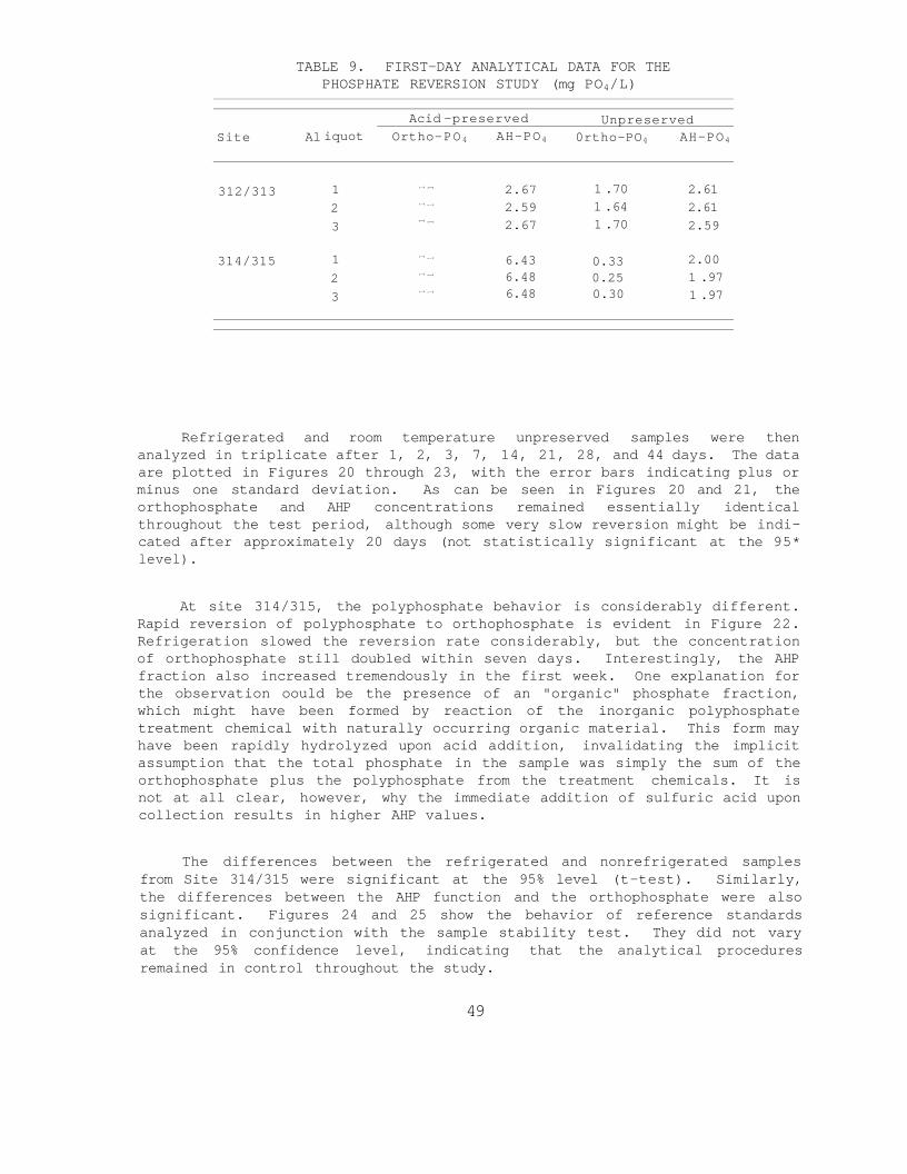
Steel Specimens 28 8 Water Usage at Test Sites 31 9 First-Day Analytical Data for the Phosphate Reversion
Study (mg PO4L) 49 10 Comparison of Some Filtered and Unfiltered Standing
Trace Metal Concentrations for Site 305 (Copper Pipe Loop) 60
11 Comparison of Some Filtered and Unfiltered Standing Trace Metal Concentrations for Site 306 (Galvanized Pipe Loop) 60
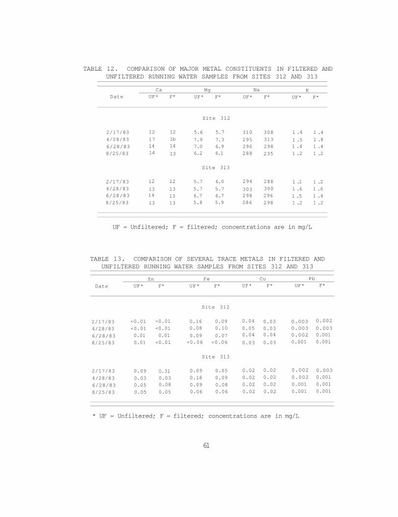
12 Comparison of Major Metal Constituents in Filtered and Unfiltered Running Water Samples from Sites 312 and 313 61
13 Comparison of Several Trace Metals in Filtered and Unfiltered Running Water Samples from Sites 312 and 313 61
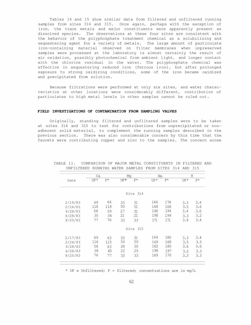
14 Comparison of Major Metal Constituents in Filtered and Unfiltered Running Water Samples from Sites 314 and 315 62
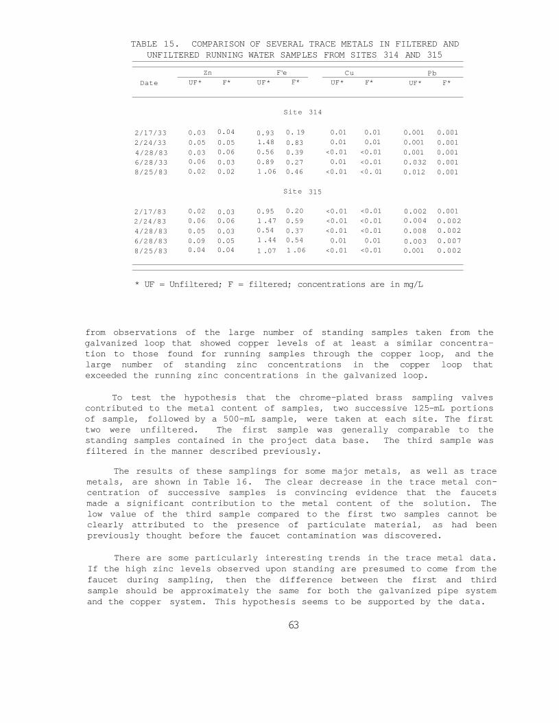
15 Comparison of Several Trace Metals in Filtered and Unfiltered Running Water Samples from Sites 314 and 315 63
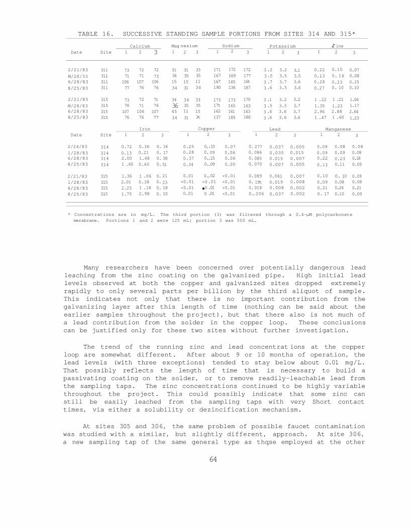
16 Successive Standing Sample Portions from Sites 314 and 315 64
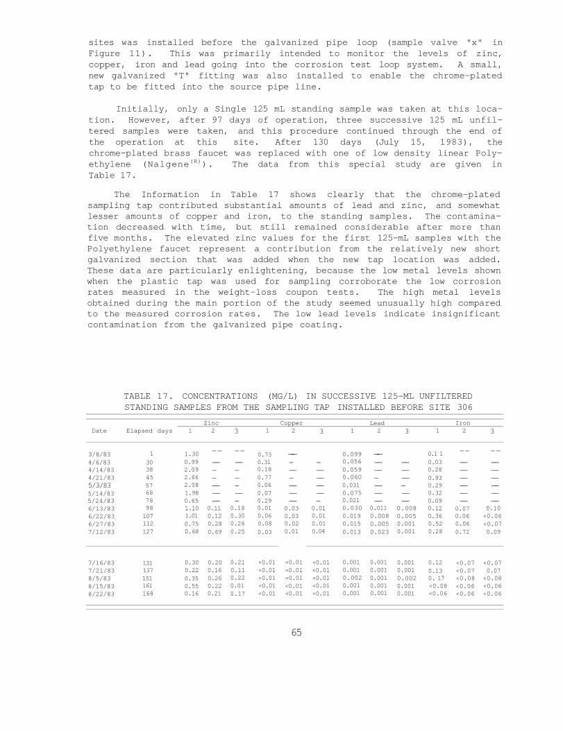
17 Concentrations (mgL) in Successive 125-mL Unfiltered Standing Samples from the Sampling Tap Installed before Site 306 65
18 Compounds Identified in Corrosion Specimen Deposits by X-ray Diffraction 73
19 Observed Corrosion Rates for Copper Specimens (mdd) bull 76 20 Observed Corrosion Rates for Galvanized Steel
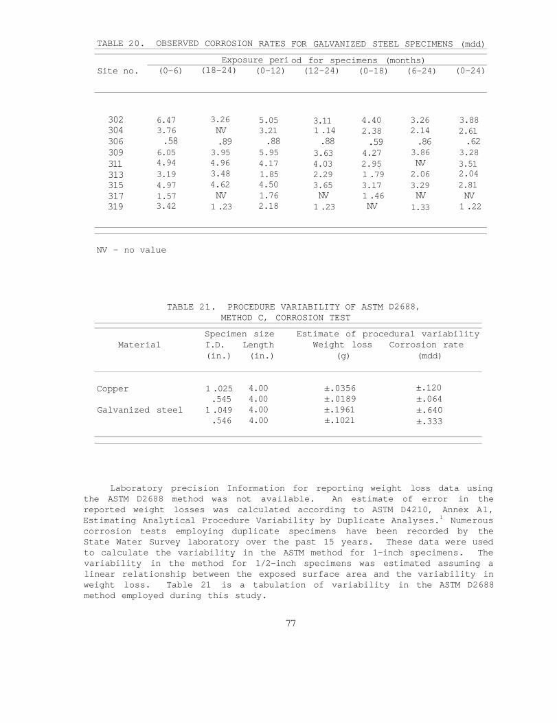
Specimens (mdd) 77
xii
TABLES (concluded)
Number Page
21 Procedure Variability of ASTM D2688 Method C Corrosion Test 77
22 Swedish Flow Rate Regulations for Copper Tube 90 23 Effect of Water Flow on Corrosion Rate 91 24 Effect of Water Flow on Metal Concentrations in Water 91 25 Analytical Independent Variables Considered in the
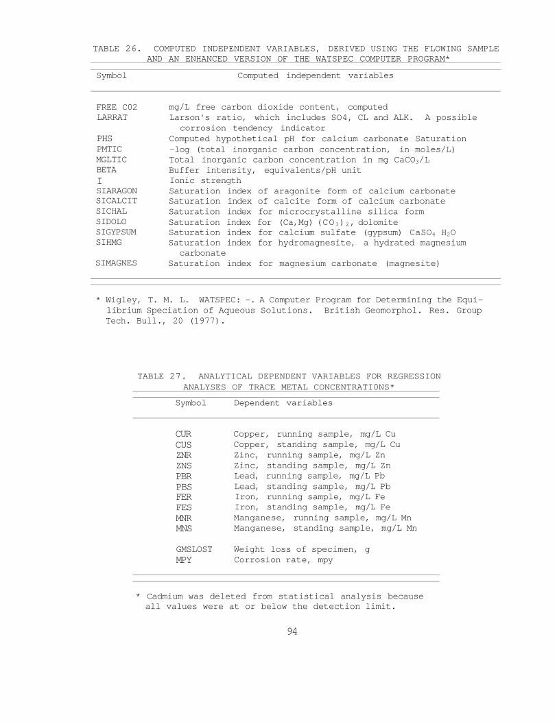
Regression Analyses for Weight Loss Correlations 93 26 Computed Independent Variables Derived Using the
Flowing Sample and an Enhanced Version of the WATSPEC Computer Program 94
27 Analytical Dependent Variables for Regression Analyses of Trace Metal Concentrations 94
28 Variables Found Significant in Predicting the Concentra-tion of Copper in the Running Samples from Each Site 96
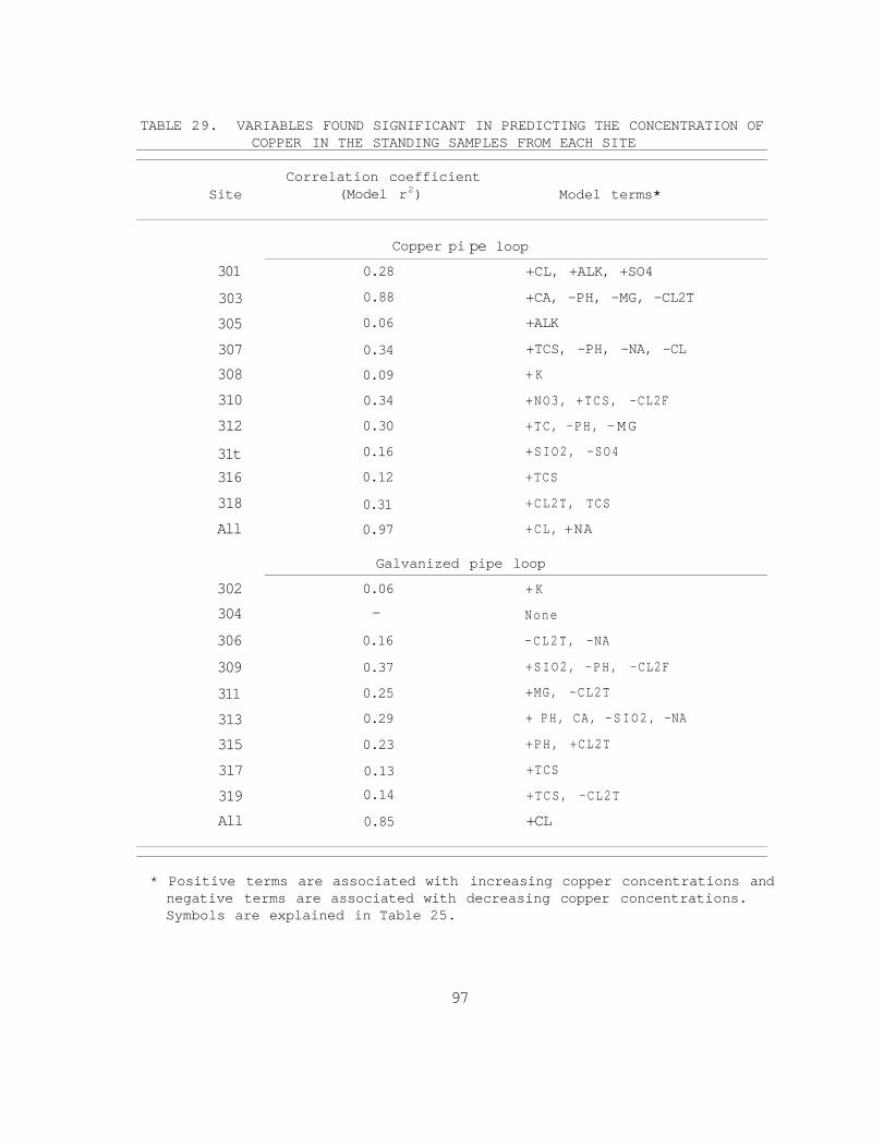
29 Variables Found Significant in Predicting the Concentra-tion of Copper in the Standing Samples from Each Site 97
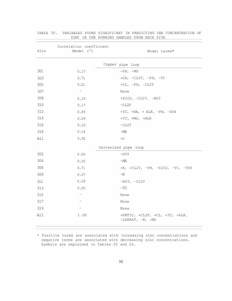
30 Variables Found Significant in Predicting the Concentra-tion of Zinc in the Running Samples from Each Site 98
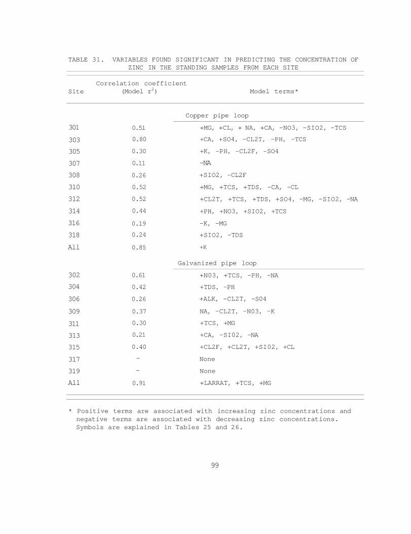
31 Variables Found Significant in Predicting the Concentra-tion of Zinc in the Standing Samples from Each Site 99
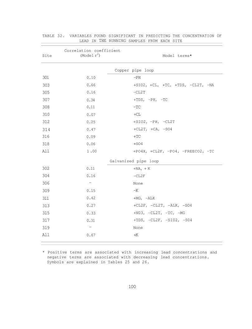
32 Variables Found Significant in Predicting the Concentra-tion of Lead in the Running Samples from Each Site 100
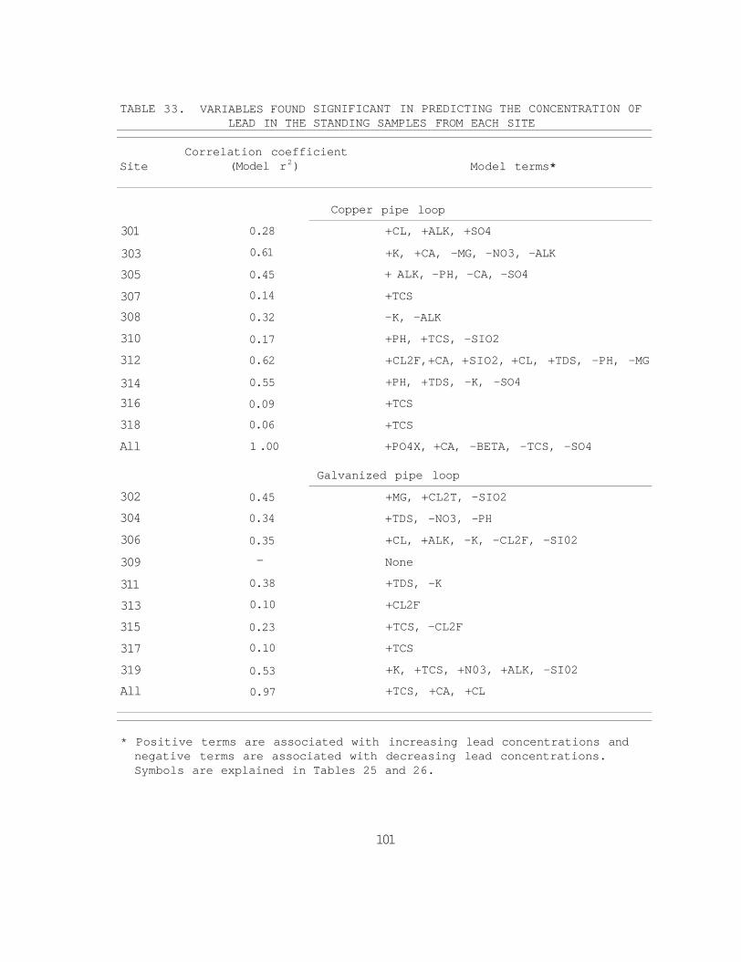
33 Variables Found Significant in Predicting the Concentra-tion of Lead in the Standing Samples from Each Site 101
34 Linear Regression Model for the Weight Loss of Copper Systems With No Site-Specific Terms 107
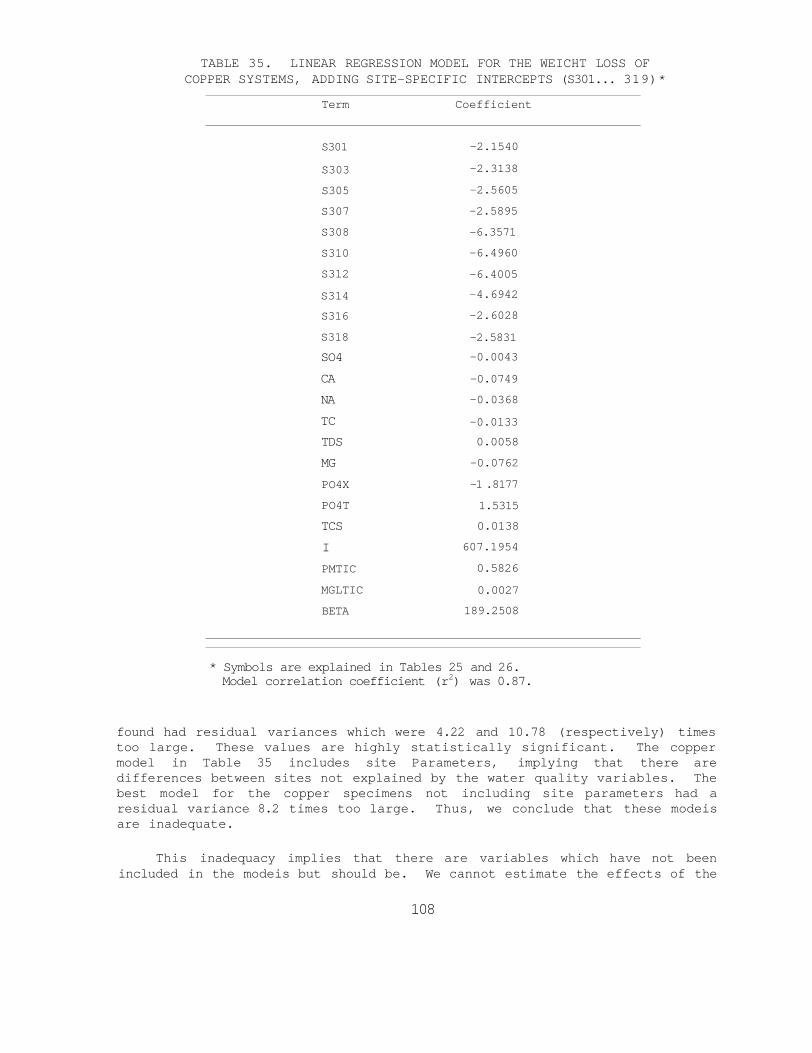
35 Linear Regression Model for the Weight Loss of Copper Systems Adding Site-Specific Intercepts (S301319) 108
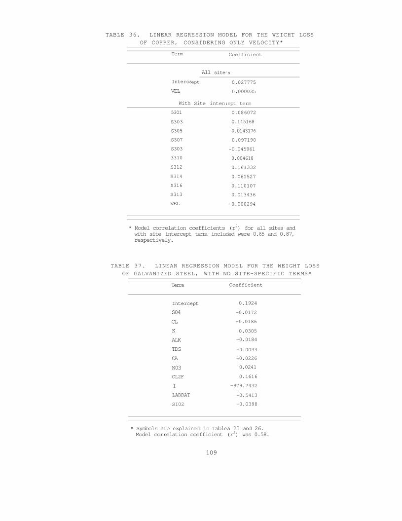
36 Linear Regression Model for the Weight Loss of Copper Considering Only Velocity 109
37 Linear Regression Model for the Weight Loss of Galvanized Steel With No Site-Specific Terms 109
38 Frequency with Which Samples Exceed the MCL for Trace Metals 113
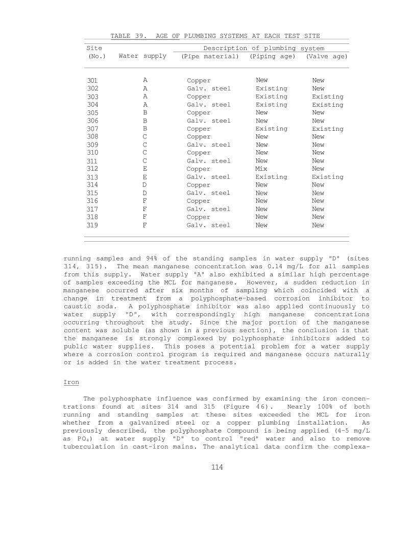
39 Age of Plumbing Systems at Each Test Site 114 40 Composition of Deposits in Corrosion Specimens Water
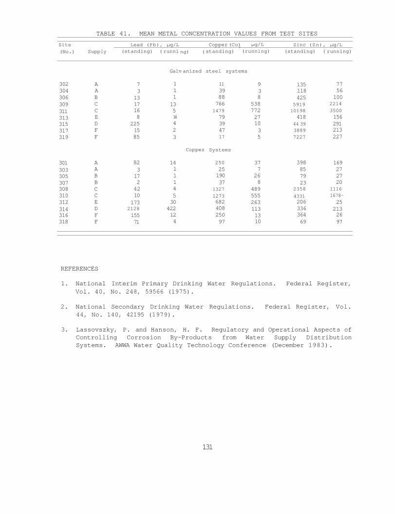
Supply C 119 41 Mean Metal Concentration Values from Test Sites 131
xiii
ACKNOWLEDGMENTS
The authors wish to acknowledge the valuable contributions made to the corrosion study by Marvin C Gardeis US Environmental Protection Agency Project Officer and the following staff of the Illinois State Water Survey Russell Lane original principal investigator Kent Smothers and Dwayne Cooper field personnel Dr Michael Barcelona Head of Aquatic Chemistry Pam Beavers secretary and the Analytical Chemistry Laboratory Unit headed by Mark Peden
In addition Dr James Rigsbee Department of Metallurgy and Engineering at the University of Illinois provided technical assistance in evaluating data
The conscientious efforts of the individuals responsible for collecting the samples making the water tests at the sites and shipping the samples to the State Water Survey Laboratory are greatly appreciated Without their Cooperation the corrosion study could not have been completed The following individuals and organizations contributed to this effort
John Swayze Superintendent of Water Operations Colleen Ozment Superintendent of Central Laboratory City of Carbondale Carbondale IL
John Meister Environmental Engineer Pollution Control Department Southern Illinois University Carbondale IL
George Russell Vice-President Andy Kieser Production Manager Northern Illinois Water Corporation Champaign IL
Jack Anderson Maintenance Engineer Gerald Anderson Chief Engineer Dwight Correctional Center Dwight IL
Martin Cornale Chief Engineer William Call Plant Engineer William Fox Developmental Center Dwight IL
xiv
James Dransfeldt Water Superintendent City of Dwight Dwight IL
Bernard Birk Chief Engineer McFarland Mental Health Center Springfield IL
LaVerne Hudson Manager Michael Battaglia Plant Engineer City of Springfield Springfield IL
xv
SECTION 1
INTRODUCTION
SCOPE AND OBJECTIVES
The principal objective of the corrosion study was to determine the influence of water quality on the corrosion rates of galvanized steel and copper pipe specimens installed in the potable water Systems of residences and large buildings Six public water supplies in Illinois were selected for the study representing both ground-water and surface water sources Each water supply used various water treatment methods which included lime-softening ion exchange softening polyphosphate and Silicate programs
Nineteen corrosion test sites were selected for the study and were located in different sections of the distribution system of each water supply The corrosion rates for galvanized steel and copper specimens were determined by a weight loss method (ASTM D2688 Method C) Seven corrosion specimens were exposed for set intervals during the two years each site was in operation
A second objective of the corrosion study was to monitor the trace metal concentrations contributed by galvanized steel and copper plumbing materials to the drinking water Total zinc copper lead iron manganese and cadmium concentrations were determined for both running and standing samples collected from taps in the buildings where corrosion test sites were located Water samples were collected for a complete chemical analysis at 2-week intervals throughout the corrosion study
On completion of the data collection phase of the corrosion study the water quality corrosion and trace metal data were evaluated by statistical methods in an attempt to identify significant factors influencing the corrosivity of water Laboratory studies were conducted to identify par-ticulate and soluble corrosion products and to measure the contribution of brass valves to the total metal concentrations observed in drinking water
BACKGROUND
Corrosion has been a long-standing and serious problem in public water supply distribution Systems Hudson and Gilcreas1 estimated in 1976 that nearly half of the 100 major US cities distribute a corrosive water The Potential health effects of corrosion led to federal regulations establish-ing maximum contaminant levels (MCLs) for certain metal concentrations in
1
drinking water23 As stated in the regulations water supplies should be noncorrosive to all plumbing materials Though some researchers45 have attempted to identify or predict waters that are corrosive none have found a universally acceptable method for identifying a corrosive water that takes into consideration all piping materials and conditions of exposure Some of the controversy over establishing the Secondary Drinking Water Regulations to the Safe Drinking Water Act was in defining noncorrosive water and acceptable methods for determining the corrosivity of water Originally the US Environmental Protection Agency (USEPA) considered the use of the Langelier Index67 the Aggressive Index8 and the Ryznar Index9 for pre-dicting the corrosion tendencies of water Because these calcium-carbonate-based indices were not reliable indicators for corrosivity the USEPA decided to require more extensive monitoring of the materials of construction water chemistry and corrosion products in the public water supplies
Two materials that have found widespread use in plumbing Systems are copper and galvanized steel pipe Experience has shown that both materials offer good corrosion resistance to drinking water when the materials are properly selected and installed However many corrosion failures have been documented for copper1011 and galvanized steel1213 piping The corrosion impact of these materials on water quality has not been adequately investi-gated Brass valves lead-based solders bronze meters or other fittings associated with copper and galvanized steel may also make a significant contribution to the soluble or particulate metal concentrations in drinking water
The Illinois State Water Survey (ISWS) has been determining the corroshysion rates for copper and galvanized steel in public water supplies for many years The ASTM D2688 Method C (Standard Method for Measuring the Corrosivshyity of Water14) was developed by the ISWS in 1955 and has been used exten-sively in state facilities The method has been a reliable indicator for corrosion andor scale deposition and has been used primarilyto indicate the effectiveness of various water treatment programs Attempts were made by the ISWS to correlate the mineral content of the water supplies with the observed corrosion rates for copper and galvanized steel The correlations met with only limited success because several important chemical parameters were not determined or evaluated
The project outlined in the previous section grew out of the common interest of the USEPA and the ISWS in (1) developing correlations between water chemistry and the corrosion rates of copper or galvanized steel and (2) investigating the impact of these piping materials on water quality
PROJECT DESIGN AND CONSTRAINTS
The design of a corrosion project is often determined by the theoreti-cal concerns of the research scientist or by the practical concerns of the corrosion engineer or environmental scientist Because the research scientist is searching for a better understanding of basic corrosion mecha-nisms short-term studies are usually conducted in the laboratory where the
2
corrosion environment can be closely controlled The corrosion engineer or environmental scientist searches for Information on the corrosion of materi-als as it affects equipment life or water quality Since laboratory research does not often translate well into actual field experiences long-term field studies in real Systems are preferred by the corrosion engishyneer or environmental scientist
This latter approach was used in this study to investigate corrosion Problems in actual plumbing Systems of buildings as influenced by the water quality of various Illinois water supplies The corrosion rate for metals in public water supplies is usually low because the water source has been treated to reduce the corrosivity or because the corrosivity of the water source is naturally low Therefore a 2-year study was considered the mini-mum time needed to obtain adequate and reliable corrosion measurements and to collect sufficient water chemistry data
The planned interval corrosion test method of Wachter and Treseder15 was considered the best procedure for evaluating the effect of time and the effect of the corrosivity of the water on the corrosion of metals Corrosion specimens prepared according to ASTM D2688 Method C are easily adapted to the planned interval method of evaluation Installing two of the ASTM corshyrosion test assemblies (each containing two corrosion specimens) at each test site and replacing each of the specimens in turn with another specimen at 6-month intervals during the corrosion study would provide seven weight loss measurements each representing a different time period during the study The use of duplicate specimens was considered and would have provided useful Information but the additional plumbing and handling costs prohib-ited their installation Copper and galvanized steel were the two materials selected for testing since they represented the major plumbing materials installed in buildings Several solders copper alloys and steel were other materials considered for testing but they were rejected because of increased project costs
The complete water chemistries for many water supplies are required if significant correlations are to be found between the water quality Parameters and the corrosion rates of metals Both inhibiting and aggresshysive influences of various constituents on the corrosivity of drinking water have been reported The chemical constituents commonly cited as influencing the corrosivity of water are calcium alkalinity pH carbon dioxide sulshyfate chloride dissolved oxygen silica temperature and dissolved solids456 Other constituents such as chlorine organics and polyphos-phates are also suspected to influence the corrosivity of water The inter-action among these various influences can be observed only by determining the corrosivity of water in real distribution Systems
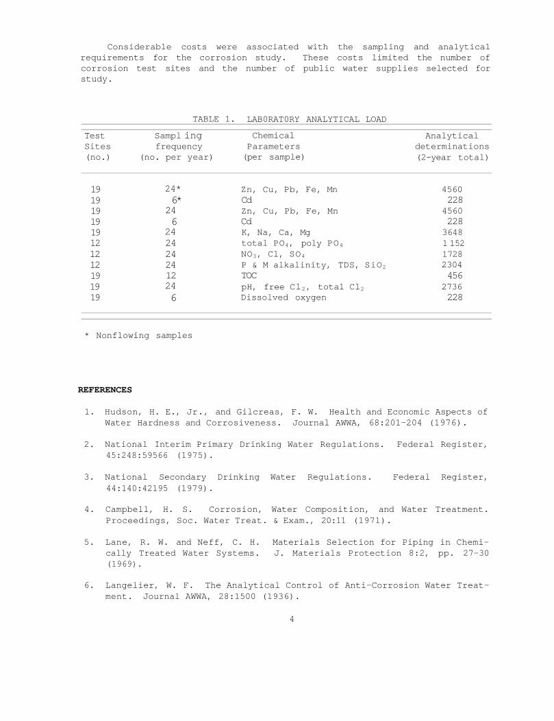
The analytical program of the corrosion study was designed to determine all the major chemical constituents in addition to those known to influence the corrosivity of water The metal concentrations were to be determined for running and standing water samples The complete water chemistry of each water supply was considered essential for future data evaluation Table 1 summarizes the laboratory analytical load for determining the essential constituents for each sampling site
3
Considerable costs were associated with the sampling and analytical requirements for the corrosion study These costs limited the number of corrosion test sites and the number of public water supplies selected for study
Nonflowing samples
REFERENCES
1 Hudson H E Jr and Gilcreas F W Health and Economic Aspects of Water Hardness and Corrosiveness Journal AWWA 68201-204 (1976)
2 National Interim Primary Drinking Water Regulations Federal Register 4524859566 (1975)
3 National Secondary Drinking Water Regulations Federal Register 4414042195 (1979)
4 Campbell H S Corrosion Water Composition and Water Treatment Proceedings Soc Water Treat amp Exam 2011 (1971)
5 Lane R W and Neff C H Materials Selection for Piping in Chemi-cally Treated Water Systems J Materials Protection 82 pp 27-30 (1969)
6 Langelier W F The Analytical Control of Anti-Corrosion Water Treatshyment Journal AWWA 281500 (1936)
4
Test Sites (no)
19 19 19 19 19 12 12 12 19 19 19
Sampl TABLE 1
ing frequency
(no per
24 6 24 6
24 24 24 24 12 24 6
year)
LAB0RAT0RY ANALYTICAL Chemical Parameters (per sample)
Zn Cu Pb Fe Mn Cd Zn Cu Pb Fe Mn Cd K Na Ca Mg total PO4 poly PO4 NO3 Cl SO4 P amp M alkalinity TDS TOC pH free Cl2 total Cl2 Dissolved oxygen
LOAD
SiO2
Analytical determinations (2-year total)
4560 228 4560 228 3648 1 152 1728 2304 456 2736 228
7 Larson T E and Buswell A M Calcium Carbonate Saturation Index and Alkalinity Interpretations Journal AWWA 341667 (1942)
8 AWWA Standard for Asbestos-Cement Pressure Pipe 4 in through 24 in for Water and Other Liquids AWWA C400-77 AWWA Denver Colorado (1977)
9 Ryznar JW A New Index for Determining Amount of Calcium Carbonate Scale Formed by Water Journal AWWA 36472 (1944)
10 Cruse H and Pomeroy R D Corrosion of Copper Pipes Journal AWWA 8479 (1974)
11 Lucez V F Mechanism of Pitting Corrosion Copper in Supply Waters Brit Corrosion Jour 2175 (1967)
12 Britton S C The Resistance of Galvanized Iron to Corrosion by Domestic Water Supplies J Soc Chem Industry 119 (1936)
13 Kenworthy L and Smith M D Corrosion of Galvanized Coatings and Zinc by Waters Containing Free Carbon Dioxide J Inst Metals 70463 (1944)
14 ASTM Book of Standards D2688 Method C 31162 (1980)
15 Wachter A and Treseder R S Corrosion Testing Evaluation of Metals for Process Equipment Chem Eng Progr 436315 (1947)
5
SECTION 2
CONCLUSIONS
METHOD OF CORROSION MEASUREMENT
Corrosion measurements were determined by modified ASTM corrosion test assemblies that were installed in the actual plumbing Systems of buildings or were part of a simulated piping loop The ASTM D2688 corrosion test assembly was reduced in size from 1 inch to 12 inch to conform with the nominal pipe dimensions encountered in household plumbing Systems The smaller test assemblies were successful in simulating the actual surface conditions found in piping without undue distortion of flow Visual inspec-tion of corrosion specimens and associated piping in the test loop after 2 years of exposure showed that the interior surfaces were identical in appearance
The simulated loops were designed to approximate the usage water velocity material exposure and stagnation periods of water in household Systems and provided reliable control of water flow and stagnation inter-vals during operation Standing samples were collected at times convenient to sampling personnel and were not biased by uncontrolled usage or by leaking plumbing fixtures which occurred in household Systems The use of test loops also circumvented service disruptions during installation and removal of corrosion specimens at the test sites Since each test loop was identical in design the piping materials and exposed surfaces were equiva-lent at each site employing the test loops The use of both simulated test loops and household plumbing for the corrosion study provided a mix of old and new plumbing materials for comparison purposes
The planned interval test method was successfully used in this study to evaluate the corrodibility of copper and galvanized steel and to evaluate the corrosivity of the water supply A decrease in the corrodibility of both metals was observed which was attributed to the formation of surface films In the less aggressive water supplies the corrosion rates of the metals were very low and remained relatively constant
The weight loss data for galvanized steel specimens were more erratic than similar data for copper specimens This was attributed to the spotty nature of the surface film observed on galvanized steel in contrast to the surface film on copper which appeared uniform and continuous The use of multiple corrosion specimens for each exposure period is recommended for future studies of galvanized steel corrosion The minimum exposure period for a Single reliable corrosion measurement in the selected water supplies
6
was determined to be 12 months for copper and 18 months for galvanized steel
VARIABILITY OF WATER QUALITY IN PUBLIC SUPPLIES
The water supplies selected for the study represented a diversity of treatment processes water quality and corrosion control programs Ground-water and surface water sources were chosen to provide a broad range of mineral concentrations The preliminary evaluation of these supplies indicated that the quality of the distribution water had remained consistent for several years prior to the study However significant variations in water chemistry were observed in samples collected biweekly over a 2-year period from each water supply
The observed upsets in water quality were caused by equipment failures modification of treatment programs or routine operational procedures employed by the water supply Both random and cyclic variations in water quality were observed Surface water supplies experienced normal cyclic variations in quality each year due to seasonal changes
Chemical constituents that varied significantly in one or more of the water supplies were chloride sulfate nitrate alkalinity pH sodium calcium magnesium chlorine dissolved solids inorganic phosphate dis-solved oxygen and organic carbon Some of these constituents (ie pH alkalinity) are known to influence the corrosivity of water while the effects of some others are unknown Although it was not evident in this study the Variation in water chemistry may adversely influence the corrosshyivity of a water supply Additional corrosion studies are required to iden-tify and document the effect of many of the chemical constituents on the corrosion of metals in water
Random or cyclic variations in water quality occured more frequently than anticipated It was found that the frequency with which samples should be collected must be modified to detect excursions in water quality The sampling frequency for routine monitoring of drinking water outlined by EPA guidelines is not adequate for this purpose The effect of these excursions in water chemistry on the corrosivity of water requires further study
EFFECT OF WATER QUALITY ON CORROSION RATES
Major fluctuations in water chemistry of short duration did not sig-nificantly change the corrosivity of the water supplies studied Any effects due to a change in concentration of specific chemical constituents known to influence corrosion were apparently averaged out by the long-term corrosion tests
A reduction in corrosivity was observed in one supply when a zinc poly-phosphate corrosion inhibitor program was replaced during the study with a pH control program A difference in corrosivity was observed within the distribution Systems of some supplies although there was no evidence of a
7
significant change in water chemistry Water velocity was suspected to be responsible for the difference in copper corrosion in one instance
Corrosion of galvanized steel increased at one location under stagnant water conditions although copper corrosion was not influenced Very low corrosion rates were observed for both metals during normal patterns of water usage
The least aggressive water supply to copper materials was characterized by a low alkalinity and high pH dissolved oxygen chlorine and nitrate content Copper corrosion rates ranged from 04 to 02 mdd for 6-month and 24-month exposure intervals respectively The most aggressive water supply experienced copper corrosion rates from 36 to 14 mdd for the respective exposure intervals The distinguishing water quality characteristics of this supply were very high concentrations of chloride sulfate and sodium
The water supply least aggressive to galvanized steel was a lime-soda softened supply in which the Langelier Index was maintained near +04 with a moderate mineral content Corrosion rates ranged from 06 to 09 mdd for all 7 specimens in this supply The most aggressive water had corrosion rates ranging from 63 to 38 mdd for 6-month and 24-month exposure intershyvals respectively
EFFECTS OF CORROSION ON TRACE METAL CONCENTRATIONS
In all the samples collected during the study iron concentrations exceeded the maximum contaminant level (MCL) in 256 of the standing samples and 160 of the running samples Manganese concentrations were found to exceed the MCL in 145 and 116 of the standing and running samples respectively The naturally occurring iron or manganese content of the water source was found to be more significant than corrosion processes or water quality in influencing the total iron or manganese concentration The presence of polyphosphate in the water supplies was observed to complex both iron and manganese maintaining the concentrations above the MCL in some supplies
Cadmium concentrations were found to be very low in all samples both running and standing Most samples were below the minimum detection limit of 03 μgL for cadmium The MCL for cadmium was not exceeded by any sample collected during the study with the maximum observed value being 48 μgL cadmium
The zinc copper and lead concentrations of the water samples were found to be associated with corrosion in Systems contalning either copper or galvanized steel plumbing materials although multiple linear regression modeis were unable to identify any significant relationships between metal concentrations and the water quality
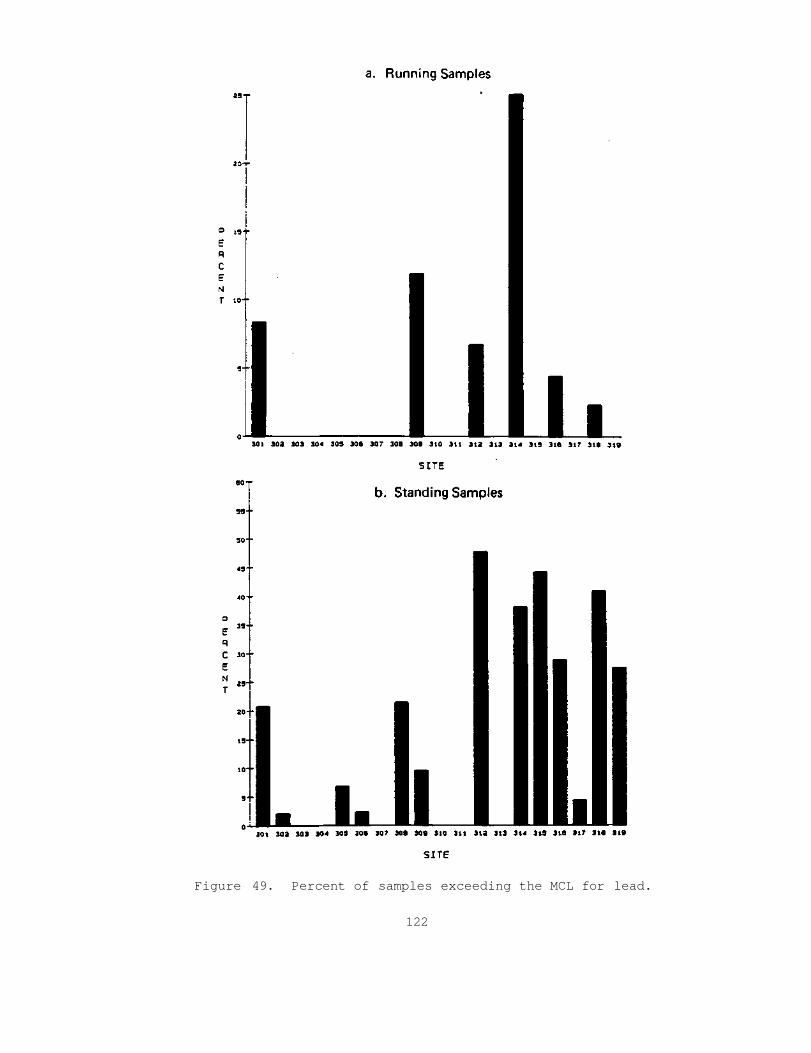
The maximum contaminant level for lead was exceeded in 171$ of the standing samples and in 31$ of the running samples The running samples exceeding the MCL for lead were collected from five copper plumbing Systems
8
and from one galvanized plumbing system The corrosion of lead-tin solder and the brass sampling valves was responsible for the lead content of samples
Copper concentrations exceeded the MCL in 106 of the standing samples and 45 of the running samples while zinc concentrations exceeded the MCL in 118 of the standing samples and 22 of the running samples
The concentration of copper zinc and lead of both standing and running samples generally decreased over the 24-month sampling period and approached an apparent mean concentration plateau around which the metal concentrations fluctuated Prior to reaching the concentration plateau the metal content from sample to sample was observed to fluctuate over a wide concentration range characterized by concentration spikes attributed to particulate corrosion products The overall distribution of the trace metal concentrations appeared to be approximately log-normal rather than Gaussian
At six selected sampling sites the total metal concentrations in fil-tered and unfiltered samples were studied and little evidence of any parshyticulate metal species in the water samples was found Contribution by particulate species to high metal concentrations in samples from other test sites could not be ruled out
A dependency of the trace metal concentrations in samples upon the length of time during which the plumbing materials were exposed to the water was observed Samples from sites where plumbing materials had 15 years or more of exposure attained the concentration plateau very quickly while samples from some newly installed plumbing Systems required several months to approach the concentration plateau
In one water supply the metal concentrations were observed to increase sharply during the latter stages of the study after apparently attaining stable concentrations Similar observations in the Seattle system were observed by Sharrett et al1 although the possible metal contribution by sampling valves was not considered
The total metal concentrations in samples were influenced by other factors such as piping configurations prior to the sampling valve and rate of flushing prior to sample collection
STATISTICAL ASSOCIATION OF WATER QUALITY VARIABLES AND CORROSION RATES
The multiple linear regression modeis did not identify any significant relationships among the many independent water quality variables and the trace metal concentrations of water samples or the weight loss of corrosion specimens The inadequacy of the modeis was attributed to four potential causes (1) important variables of the water were not measured (2) the independent water quality variables were not constant between sampling dates (3) there were interactions between two or more variables that were not integrated into modeis and (4) the variables needed to be transformed
9
into other terms The latter two causes are considered the most plausible and require further study
There were too many relationships to examine and too much variability between sites and within sites for an uncontrolled field study to reach many definitive conclusions No Single relationship was strong enough to rise above all the other variables to be identified The study was important because it provides strong evidence that there are many more factors and interrelationships affecting corrosion rates than have been taken into account by a simple linear regression model
No attempt was made in this study to evaluate the corrosion rate or trace metal leaching data within the framework of a solution chemical model In order to do so a complete chemical analysis of the standing samples would have been required and the stagnation time necessary to reach the solubility equilibrium would have had to be determined and adjusted accordingly
CONTRIBUTION OF TRACE METALS BY SAMPLING VALVES
Field and laboratory studies were conducted to test the hypothesis that the chrome-plated brass sampling valves were making a significant contribu-tion to the metal content of the water samples A clear decrease in the concentration of lead zinc and copper occurred in successive samples taken from brass sampling valves at field sites providing convincing evidence that the valves were contributing significantly to the metal content of samples The field data also indicated that lead was not originating in the galvanized layer of the galvanized steel loop or from the lead-tin solder of the copper loop at these sites
Contamination of samples by the brass valves decreased with time in a study at another site but remained substantial after more than five months of testing Substitution of a Polyethylene sampling valve for the brass sampling valve sharply reduced the lead and zinc concentrations in the samples providing further evidence of contamination by the brass valve
The effect of time on the trace metal content of water due to leaching within the valve body was investigated in the laboratory Six identical brass faucets were filled to capacity with either deionized water or tap water and were drained after 2k hours exposure to check the metal content of successive samples collected over a 14-day period Leaching of cadmium was not significant all concentrations were near the analytical detection limit Iron concentrations decreased rapidly to the detection limit within five days Copper concentrations decreased from approximately 10 mgL Cu to 01 mgL Cu for both deionized water and tap water Zinc concentrations were above 10 mgL Zn in the first sample and gradually decreased to 1 mgL Zn in the last sample Lead concentrations were extremely high in the deionized water samples ranging from 100 mgL Pb in the first sample to 1 mgL in the last sample Tap water samples were also above the MCL for lead decreasing from approximately 1 mgL Pb to 01 mgL Pb in consecutive samples during the 14-day study
10
ADDITIONAL LABORATORY STUDIES
A study on the effect of temperature and time on the hydrolysis of polyphosphate during sample storage revealed that the reversion rates to orthophosphate were influenced by unaccounted-for factors For samples from water supply E the orthophosphate and acid hydrolyzable phosphate (AHP) concentrations did not change significantly whether stored for 45 days at room temperature or refrigerated However for water supply D both the orthophosphate and AHP fractions increased in concentration under the same storage conditions as those of supply E When samples from supply D were immediately preserved with sulfuric acid the AHP concentrations were much greater than the AHP concentrations found in unpreserved samples Due to some unknown influence the AHP fraction was observed to increase in conshycentration although the concentration was not anticipated to change Inorganic phosphate was the only form of phosphate assumed to be present in the samples
The waterside surface deposits were removed from a few corrosion speci-mens exposed for two years in the water supplies and were examined by X-ray diffraction to identify specific Compounds The most interesting Compounds found in the deposits were vaterite and orthophosphate Compounds of zinc and iron The corrosion products associated with the corrosion of copper or galvanized materials (copper oxide zinc oxide and basic carbonates) were also identified in the deposits
REFERENCE
1 Sharrett A R et al Daily Intake of Lead Cadmium Copper and Zinc from Drinking Water The Seattle Study of Trace Metal Exposure Environ Res 28456 (1982)
1 1
SECTION 3
RECOMMENDATIONS
A summary of the recommendations and research needs developed from this study is listed for consideration in future investigations of similar nature
1 The trace metal content of drinking water is strongly influenced by abnormalities in the sampling process therefore sampling protocols should be developed for the specific requirements of environmental health studies corrosion studies or water quality studies The sampling valve materials piping configurations plumbing age flushing volumes flushing flow rates and stagnation intervals must be consid-ered in establishing the protocol for each type of study Flow samples collected from nonmetallic taps are recommended for moni-toring purposes in corrosion studies If equilibrium chemical modeis are to be tested to determine if they can predict or simulate the cormdash rosion or passivation behavior of the plumbing materials complete water chemistry data must be obtained for standing samples and tests should be made to ascertain the stagnation period actually required to reflect equilibrium solubility conditions
2 The impact of brass bronze and other copper alloy plumbing materials on the trace metal content of drinking water should be given high priority in future studies Chrome-plated brass faucets were found to be a major source of lead copper and zinc concentrations found in the public water supplies sampled The factors influencing the trace metal content of drinking water contributed by these materials should be examined and identified
A testing protocol should be developed to determine the leaching potenshytial of metals from faucets delivering water for human consumption and the faucets should be tested prior to marketing A certification and testing program was developed in Denmark1 which may serve as a useful model
3 The widespread application of various commercial polyphosphate chemicals to public water supplies should be critically examined The benefits of polyphosphate usage have been well documented for sequestering iron and manganese inhibiting mineral deposition and Controlling tuberculation in distribution systems However the Potential health hazards from increased metal solubility and distribushytion system problems associated with the use of polyphosphate in public water supplies have not been adequately investigated The ability of
12
polyphosphate to Sequester metals was found to be responsible for eausing iron and manganese to exceed the MCLs in some samples and for increasing the content of other trace metals during this study Polyphosphates may also increase biological activity increase deposi-tion of phosphate minerals accelerate leaching of calcium from cement-lined and asbestos-cement pipe and interfere with the formation of surface films in potable water Silicates may also exhibit similar characteristics particularly at high concentrations and should also be studied The studies should cover the identification of aqueous species contributed by the different treatment chemicals their metal complexation and hydrolysis properties and the temperature effects on the complex formation and ligand stability
4 The effect of chlorine and chloramine content in drinking water on plumbing materials requires further investigation Chlorination of public water supplies is practically a universal treatment process but varies widely in application and control practices in this country The free residual chlorine concentration has been maintained as high as 5 mgL in some Illinois water supplies In two instances the corro-sion rate of copper increased and failure of copper tube occurred at free residual chlorine concentrations of 2 mgL Trace metal concen-trations were not monitored however increased solubilization of copper by chlorine has been cited in the literature2 Because chlorine is a very strong oxidizing agent it can be expected to influence the formation or dissolution of corrosion products on metal surfaces
5 Methods should be developed for preconditioning newly installed galva-nized and copper plumbing Systems to minimize the potential health risks associated with the consumption of water containing excessive trace metal concentrations The trace metal content of water samples from new Systems decreases with tirae of exposure however the metal content may remain at high levels for several months after installa-tion Pipe materials could be treated by the manufacturer or after installation to form protective films on the surface Metaphosphates metasilicates and nitrates along with other chemicals have been used for precoating galvanized steel materials in Australia3 and France (M Dreulle Cie Royale Asturienne des Mines personal communication 1971 )
6 Extensive studies are needed to identify the interrelationships and unknown factors which influence the corrosion rate and dissolution of metals in public water supplies Field studies were inadequate for this purpose due to an excessive number of known variables unknown or missing variables lack of control of the variables and interactions among the many variables Future studies should be conducted under closely controlled laboratory conditions where a few selected variables are examined at one time As the basic chemical relationships are established a general model could be developed and extended to Systems of increasing complication
7 A standard procedure should be adopted for determining and reporting corrosion measurements in public water supplies The planned interval
13
test method which compares the weight loSS of specimens over various time frames is currently the best procedure for detecting significant changes in the corrosivity of potable water Satisfactory weight loss measurements are obtained by the ASTM D2688 method however multiple corrosion specimens are recommended for each test interval The method is adaptable to steel galvanized steel copper solder and brass materials in 12 to 2 nominal pipe dimensions
Long-term exposure of corrosion specimens is required due to the low corrosivity of most water supplies From six- to eighteen-month exposure of specimens is recommended depending on the material exposed and the corrosivity of the water supply A Single weight loss measure-ment of corrosion rate assumes a linear relationship with time but may be satisfactory when only the corrodibility of the metal is of interest in a controlled environment
8 An instantaneous corrosion rate measurement procedure capable of detecting short-term variations in the corrosivity of public water supplies should be developed Commercially available instruments could be utilized but suitable probes need to be developed which simulate the corrosion mechanisms occurring on the surface of a pipe It is unlikely that a Single probe could be made sensitive to the multitude of variables present in water supplies and could reflect pitting or scale deposition for example Instantaneous corrosion rate values would be useful in providing immediate Information on the effects of changes in treatment or variations in water quality
9 Further research is required to identify and quantify the minerals formed by corrosion or deposition on the surfaces of plumbing materials exposed to potable water X-ray diffraction studies of the surface films would assist in understanding the basic corrosion mechanisms responsible for the film formation and also would assist in differenti-ating which water chemistry parameters are significant in the process of formation This Information would be useful for designing water treatment programs which would enhance the development of protective surface films
Research is necessary to develop appropriate sampling and sample handling methodology for water-formed deposits because dehydration and oxidation can readily transform solids prior to or during X-ray analysis Correlation with the predictions made by chemical corrosion and water treatment modeis can be made only if the analyzed solids correspond to those that were formed and adhered to the pipe interior surface when covered by the water
Experience in this and other corrosion studies also indicates that the surface films are often mixtures of multiple solids and are poorly crystalline microcrystalline or amorphous These properties make simple glass slide preparation techniques and manual pattern indexing and file searching of limited value in correctly identifying the Comshypounds More emphasis is needed in this area as well
14
10 Further statistical analysis is recommended for the corrosion and analytical data presented in this report Meaningful relationships between the chemical factors and the trace metal content of samples may have been obscured by the numerous variables evaluated by multiple linear regression analyses The number of independent variables should be selectively reduced and when variables are interrelated only one of the variables should be evaluated In this study the most common inshydependent variables found in modeis predicting the metal concentrations in water samples were temperature chlorine pH silica and nitrate To a lesser extent chloride sodium potassium sulfate magnesium and alkalinity appeared in some modeis These parameters should be considered for continued modeling studies
REFERENCES
1 Nielsen K Control of Metal Contaminants in Drinking Water in Denmark Aqua No 4 (1983)
2 Atlas D J Coombs and O T Zajicek The Corrosion of Copper in Chlorinated Waters Water Res 16693 (1982)
3 Stein A The Prevention of Corrosion in Galvanized Iron Water Tanks Australian Corrosion Engineering Vol 8 No 12 (1964)
15
SECTION 4
TREATMENT PROCESSES AND QUALITY OF SELECTED WATER SUPPLIES
CRITERIA EMPLOYED FOR SELECTING WATER SUPPLIES
The corrosion investigation was limited to public water supplies within the boundaries of the state of Illinois This restriction was applied because of travel considerations Frequent Visits were anticipated to each corrosion test site and were planned to coincide with other ISWS project activities within the state
Approximately twenty public water supplies were evaluated as potential locations for the corrosion test sites The selection process considered water source treatment processes water quality and corrosion control programs all factors which influence the corrosivity of public water supplies
Abundant sources of water are found in Illinois where in 1980 public water supplies withdrew 480000000 gpd (gallons per day) of ground water and 1780000000 gpd of surface water for consumption1 The water supplies of Carbondale IL and Springfield IL were selected to be representative of typical surface water sources A deep ground-water source was selected at the state correctional center near Dwight IL and shallow ground-water sources were selected at the Champaign IL and Dwight IL public water supplies
The water quality of the distribution water for each supply was also examined and water supplies were selected which exhibited mineral concentra-tions typical of Illinois water supplies The major chemical constituents considered for this purpose were pH alkalinity total dissolved solids chloride sulfate calcium chlorine residual and dissolved oxygen Because of the limited number of water supplies which could be studied many conshystituents which influence the corrosivity of water were not employed as criteria in the selection process but were monitored throughout the corroshysion study
Common raw water treatment processes for Illinois supplies are lime softening ion exchange softening clarification filtration and aeration chlorination and fluoridation are mandated treatment programs for all water supplies and may be the only treatment applied in the case of some ground-water sources Treatment processes influence the corrosivity of water and were an important consideration for selecting specific water supplies
16
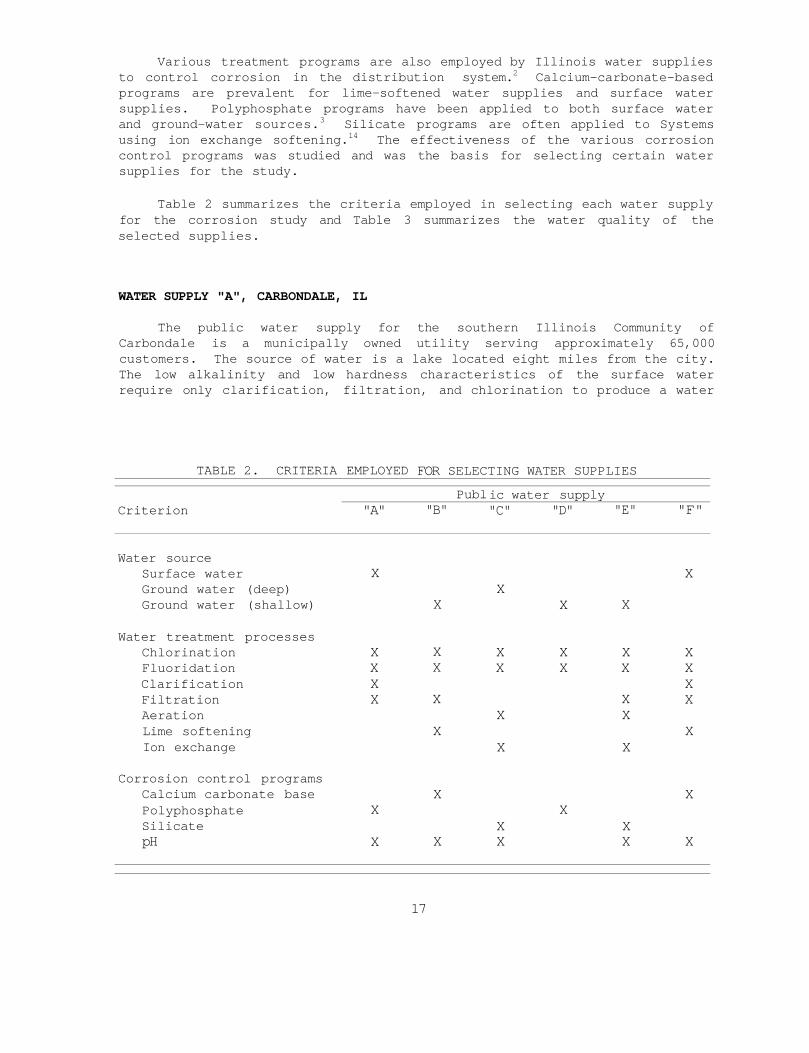
Various treatment programs are also employed by Illinois water supplies to control corrosion in the distribution system2 Calcium-carbonate-based programs are prevalent for lime-softened water supplies and surface water supplies Polyphosphate programs have been applied to both surface water and ground-water sources3 Silicate programs are often applied to Systems using ion exchange softening14 The effectiveness of the various corrosion control programs was studied and was the basis for selecting certain water supplies for the study
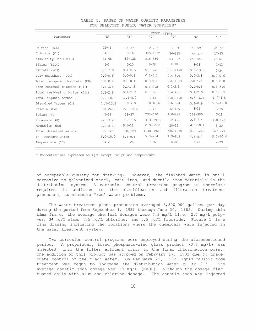
Table 2 summarizes the criteria employed in selecting each water supply for the corrosion study and Table 3 summarizes the water quality of the selected supplies
WATER SUPPLY A CARBONDALE IL
The public water supply for the southern Illinois Community of Carbondale is a municipally owned utility serving approximately 65000 customers The source of water is a lake located eight miles from the city The low alkalinity and low hardness characteristics of the surface water require only clarification filtration and chlorination to produce a water
17
TABLE 2 CRITERIA
Criterion
Water source Surface water Ground water (deep) Ground water (shallow)
Water treatment processes Chlorination Fluoridation Clarification Filtration Aeration Lime softening Ion exchange
Corrosion control programs Calcium carbonate base Polyphosphate Silicate pH
EMPLOYED
A
X
X X X X
X
X
FOR
B
X
X X
X
X
X
X
SELECTING Publ
WATER ic water C
X
X X
X
X
X X
SUPPLIES supply D
X
X X
X
E
X
X X
X X
X
X X
F
X
X X X X
X
X
X
TABLE 3 RANGE OF WATER QUALITY PARAMETERS FOR SELECTED PUBLIC WATER SUPPLIES
Concentrations expressed as mgL except for pH and temperacure
of acceptable quality for drinking However the finished water is still corrosive to galvanized steel cast iron and ductile iron materials in the distribution system A corrosion control treatment program is therefore required in addition to the clarification and filtration treatment processes to minimize red water problems
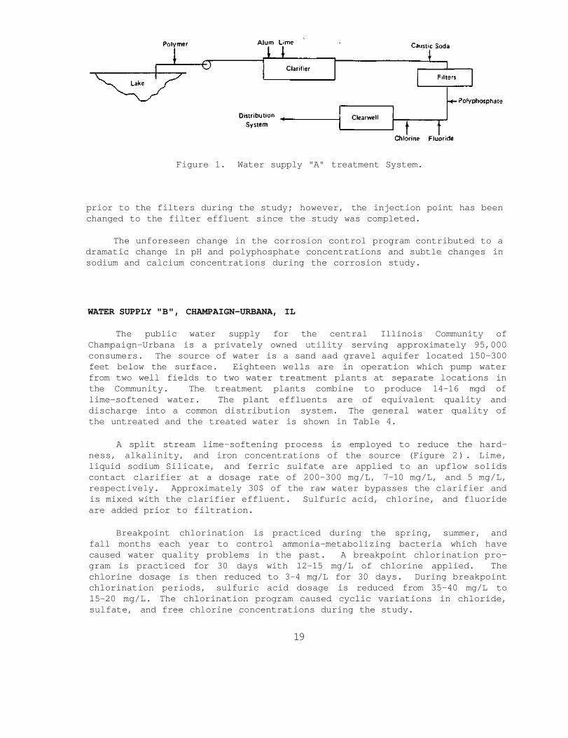
The water treatment plant production averaged 3800000 gallons per day during the period from September 1 1981 through June 30 1983 During this time frame the average chemical dosages were 73 mgL lime 20 mgL polyshyshyer 34 mgL alum 75 mgL chlorine and 05 mgL fluoride Figure 1 is a line drawing indicating the locations where the chemicals were injected in the water treatment system
Two corrosion control programs were employed during the aforementioned period A proprietary fused phosphate-zinc glass product (07 mgL) was injected into the filter effluent prior to the final chlorination point The addition of this product was stopped on February 17 1982 due to inade-quate control of the red water On February 22 1982 liquid caustic soda treatment was begun to increase the distribution water pH to 85 The average caustic soda dosage was 19 mgL (NaOH) although the dosage fluc-tuated daily with alum and chlorine dosage The caustic soda was injected
18
Parameter
Sulfate (SO4) Chloride (Cl) Alkalinity (as CaCO3) Silica (SiO2) Nitrate (NO3) Poly phosphate (PO4) Total inorganic phosphate (PO4) Free residual chloride (Cl2) Total residual chloride (Cl2) Total organic carbon (C) Dissolved Oxygen (O2) Calcium (Ca) Sodium (Na) Potassium (K) Magnesium (Mg) Total dissolved solids pH (Standard units) Temperature (degC)
A
l6-4l 4-1 1 31-68 1-5
02-30 00-06 00-08 01-26 01-29 36-105 1 5-132 98-245 5-28
06-32 10-53 95-149 60-100 4-28
B
14-57 3-16
82-128 5-10
01-05 00-01 00-01 01-1 8 01-27 1 1-82 10-70 98-145 23-37 17-25 98-11 136-229 81-91 8-26
Water C
2-293 185-1032 215-336 9-29
01-62 00-01 00-01 01-25 01-30
1-13 68-106 1-77
295-690 1 4-295 09-560 1 181-1929 73-94 7-26
Supply D
1-671 36-235 253-397 8-20
01-110 04-89 10-104 02-21 04-40 48-275 06-54 32-129 150-222 32-45 20-55 736-1270 73-82 8-21
E
49-590 52-323 266-369 8-28
03-135 00-38 08-43 01-06 04-20 53-166 04-89 8-24
261-380 08-74 40-104 830-1266 76-87 8-24
F
24-68 17-35 25-60 1-12 2-34
00-06 00-08 01-30 01-32 1 7-48 50-130 13-35 3-11
18-42 5-20
147-277 90-104
4-29
Figure 1 Water supply A treatment System
prior to the filters during the study however the injection point has been changed to the filter effluent since the study was completed
The unforeseen change in the corrosion control program contributed to a dramatic change in pH and polyphosphate concentrations and subtle changes in sodium and calcium concentrations during the corrosion study
WATER SUPPLY B CHAMPAIGN-URBANA IL
The public water supply for the central Illinois Community of Champaign-Urbana is a privately owned utility serving approximately 95000 consumers The source of water is a sand aad gravel aquifer located 150-300 feet below the surface Eighteen wells are in operation which pump water from two well fields to two water treatment plants at separate locations in the Community The treatment plants combine to produce 14-16 mgd of lime-softened water The plant effluents are of equivalent quality and discharge into a common distribution system The general water quality of the untreated and the treated water is shown in Table 4
A split stream lime-softening process is employed to reduce the hard-ness alkalinity and iron concentrations of the source (Figure 2) Lime liquid sodium Silicate and ferric sulfate are applied to an upflow solids contact clarifier at a dosage rate of 200-300 mgL 7-10 mgL and 5 mgL respectively Approximately 30$ of the raw water bypasses the clarifier and is mixed with the clarifier effluent Sulfuric acid chlorine and fluoride are added prior to filtration
Breakpoint chlorination is practiced during the spring summer and fall months each year to control ammonia-metabolizing bacteria which have caused water quality problems in the past A breakpoint chlorination proshygram is practiced for 30 days with 12-15 mgL of chlorine applied The chlorine dosage is then reduced to 3-4 mgL for 30 days During breakpoint chlorination periods sulfuric acid dosage is reduced from 35-40 mgL to 15-20 mgL The chlorination program caused cyclic variations in chloride sulfate and free chlorine concentrations during the study
19
ISWS Lab No 150853 composite of five wells concentrations expressed as mgL IEPA Lab No B28823 concentrations expressed as mgL
Figure 2 Water supply B treatment System
WATER SUPPLY C DWIGHT C0RRECTI0NAL CENTER
The Dwight Correctional Center (DCC) is a State of Illinois facility serving approximately 500 female residents in central Illinois The public water supply for DCC pumps water from two deep wells (1200 feet) which are highly mineralized and have high hydrogen sulfide and iron concentrations Well No 2 is slightly less mineralized than Well No 1 and is the well
20
TABLE 4
Parameter
Iron (Fe) Calcium (Ca) Magnesium (Mg) Sodium (Na) Silica (SiO2) Fluoride (F) Chloride (Cl) Nitrate (NO3) Sulfate (SO4) Alkalinity (as Hardness (as Ca Total dissolved
CaCO3) CO3) [ solids
QUALITY OF WATER SUPPLY
Untreated water
1 2 598 288 350 154 03 20 53 70
3280 2680 3470
B
Treated water
lt01 120 100 390 59 1 1 49 lt01 450 1000 600 1900
pumped on a daily basis Well No 1 is operated only during repairs to Well No 2 or when backup capacity is needed Average pumpage is 72000 gallons per day
The ground water is aerated and chlorinated to remove iron and hydrogen sulfide It then flows by gravity into a clear well where the iron is allowed to settle The water is then pumped from the clear well through water softeners to reduce the hardness in the distribution system which is controlled by blending approxiraately 25 hard water into the softener effluent A flow diagram and chemical injection locations are shown in Figure 3
The high dissolved solids high dissolved oxygen and low hardness of the distribution water were anticipated to increase the corrosivity of water supply C
Liquid sodium Silicate is applied to provide an 8-11 mgL (as SiO2) silica increase to inhibit corrosion Caustic soda is also applied to increase the distribution water pH to 83 to further reduce the corrosion of the system Chemicals are automatically proportioned and injected into the distribution system after softening
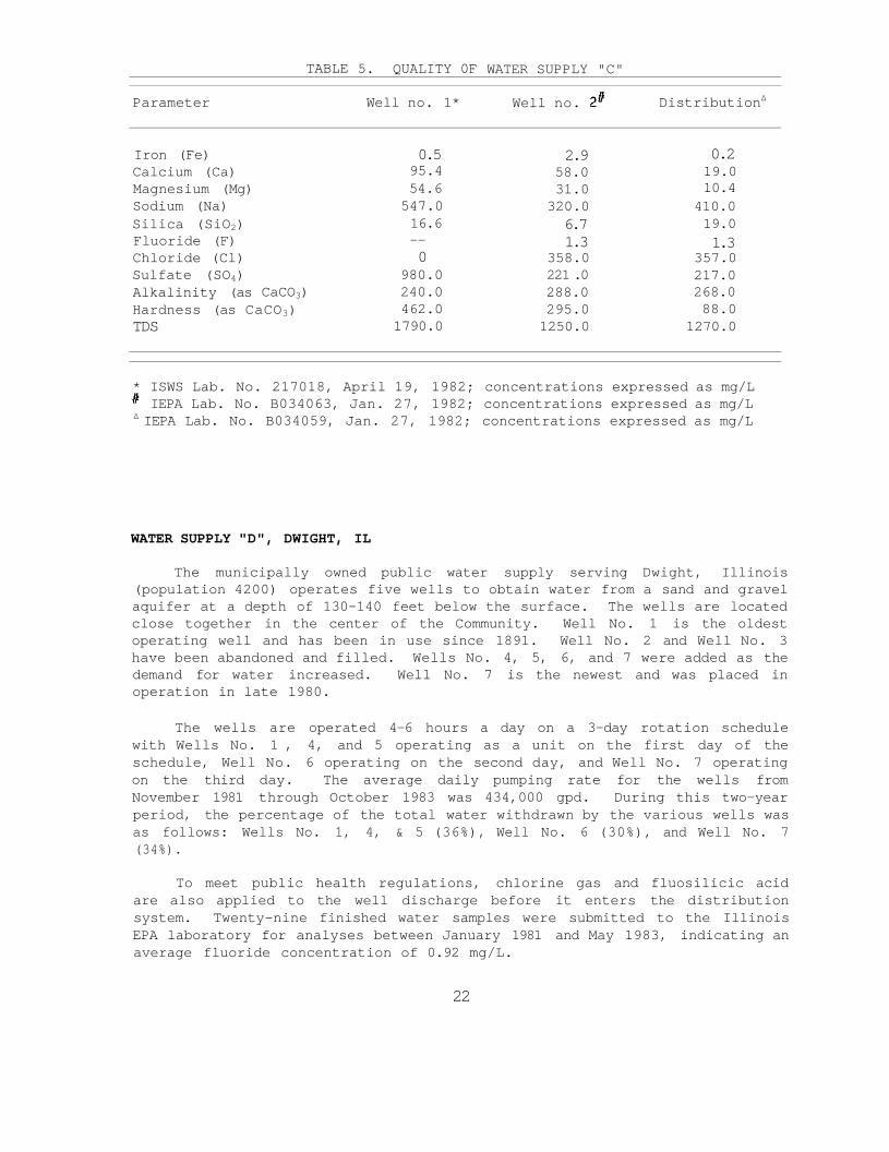
The chemical analyses of the ground water and distribution water observed for water supply C during the corrosion study are shown in Table 5 Unscheduled outages of Well No 1 occurred on two occasions which drastically altered the water quality A significant change in chloride sulfate and sodium concentrations was experienced due to use of Well No 2 during the outages
Figure 3 Water supply C treatment system
21
ISWS Lab No 217018 April 19 1982 concentrations expressed as mgL IEPA Lab No B034063 Jan 27 1982 concentrations expressed as mgL
∆ IEPA Lab No B034059 Jan 27 1982 concentrations expressed as mgL
WATER SUPPLY D DWIGHT IL
The municipally owned public water supply serving Dwight Illinois (population 4200) operates five wells to obtain water from a sand and gravel aquifer at a depth of 130-140 feet below the surface The wells are located close together in the center of the Community Well No 1 is the oldest operating well and has been in use since 1891 Well No 2 and Well No 3 have been abandoned and filled Wells No 4 5 6 and 7 were added as the demand for water increased Well No 7 is the newest and was placed in operation in late 1980
The wells are operated 4-6 hours a day on a 3-day rotation schedule with Wells No 1 4 and 5 operating as a unit on the first day of the schedule Well No 6 operating on the second day and Well No 7 operating on the third day The average daily pumping rate for the wells from November 1981 through October 1983 was 434000 gpd During this two-year period the percentage of the total water withdrawn by the various wells was as follows Wells No 1 4 amp 5 (36) Well No 6 (30) and Well No 7 (34)
To meet public health regulations chlorine gas and fluosilicic acid are also applied to the well discharge before it enters the distribution system Twenty-nine finished water samples were submitted to the Illinois EPA laboratory for analyses between January 1981 and May 1983 indicating an average fluoride concentration of 092 mgL
22
Parameter
Iron (Fe) Calcium (Ca) Magnesium (Mg) Sodium (Na) Silica (SiO2) Fluoride (F) Chloride (Cl) Sulfate (SO4) Alkalinity (as CaCO3) Hardness (as CaCO3) TDS
TABLE 5 QUALITY 0F
Well no 1
05 954 546 5470 166 --0
9800 2400 4620 17900
WATER SUPPLY C
Well no
29 580 310 3200 67 13
3580 221 0 2880 2950 12500
Distribution∆
02 190 104
4100 190 13
3570 2170 2680 880
12700
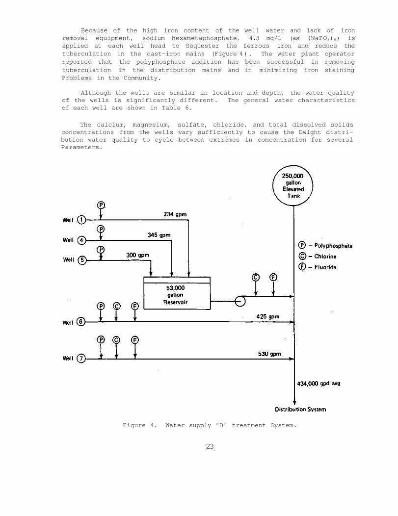
Because of the high iron content of the well water and lack of iron removal equipment sodium hexametaphosphate 43 mgL (as (NaPO3)6) is applied at each well head to Sequester the ferrous iron and reduce the tuberculation in the cast-iron mains (Figure 4) The water plant operator reported that the polyphosphate addition has been successful in removing tuberculation in the distribution mains and in minimizing iron staining Problems in the Community
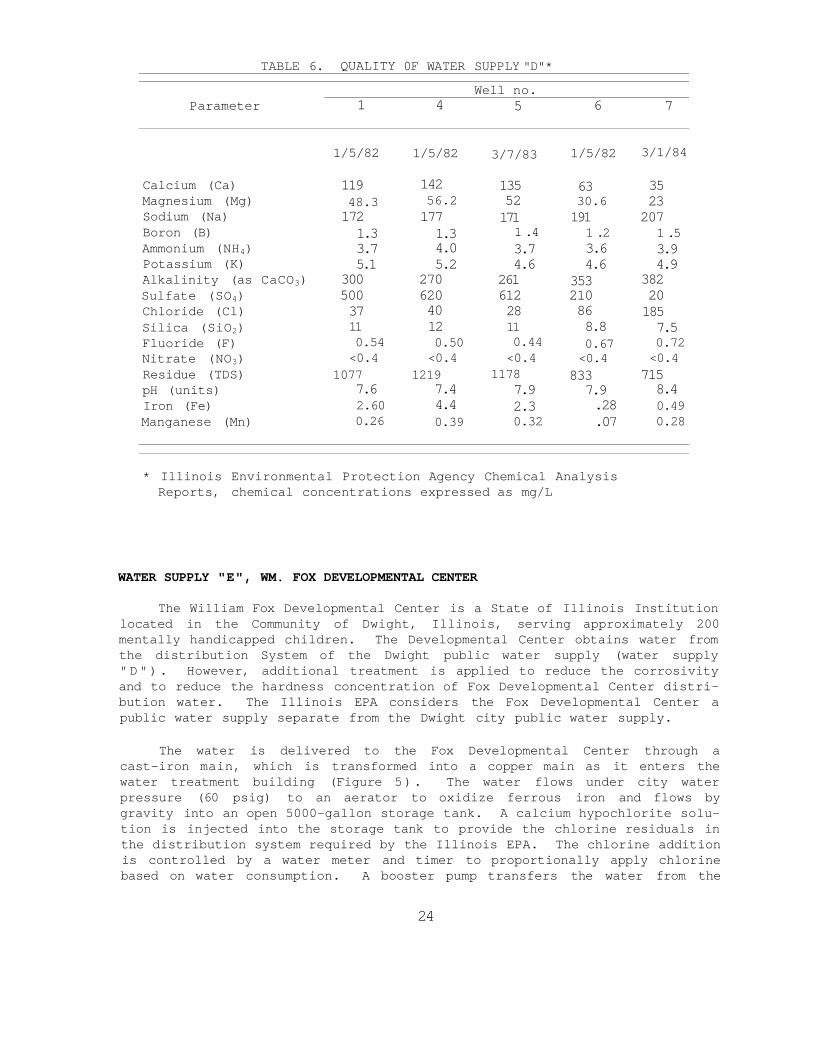
Although the wells are similar in location and depth the water quality of the wells is significantly different The general water characteristics of each well are shown in Table 6
The calcium magnesium sulfate chloride and total dissolved solids concentrations from the wells vary sufficiently to cause the Dwight distrishybution water quality to cycle between extremes in concentration for several Parameters
Figure 4 Water supply D treatment System
23
Illinois Environmental Protection Agency Chemical Analysis Reports chemical concentrations expressed as mgL
WATER SUPPLY E WM FOX DEVELOPMENTAL CENTER
The William Fox Developmental Center is a State of Illinois Institution located in the Community of Dwight Illinois serving approximately 200 mentally handicapped children The Developmental Center obtains water from the distribution System of the Dwight public water supply (water supply D) However additional treatment is applied to reduce the corrosivity and to reduce the hardness concentration of Fox Developmental Center distrishybution water The Illinois EPA considers the Fox Developmental Center a public water supply separate from the Dwight city public water supply
The water is delivered to the Fox Developmental Center through a cast-iron main which is transformed into a copper main as it enters the water treatment building (Figure 5) The water flows under city water pressure (60 psig) to an aerator to oxidize ferrous iron and flows by gravity into an open 5000-gallon storage tank A calcium hypochlorite solushytion is injected into the storage tank to provide the chlorine residuals in the distribution system required by the Illinois EPA The chlorine addition is controlled by a water meter and timer to proportionally apply chlorine based on water consumption A booster pump transfers the water from the
24
TABLE 6
Parameter
Calcium (Ca) Magnesium (Mg) Sodium (Na) Boron (B) Ammonium (NH4) Potassium (K) Alkalinity (as CaCO3) Sulfate (SO4) Chloride (Cl) Silica (SiO2) Fluoride (F) Nitrate (NO3) Residue (TDS) pH (units) Iron (Fe) Manganese (Mn)
QUALITY
1
1582
119 483 172 13 37 51
300 500 37 11 054 lt04
1077 76 260 026
0F WATER
4
1582
142 562 177 13 40 52
270 620 40 12 050 lt04
1219 74 44 039
SUPPLY D Well no
5
3783
135 52 171 1 4 37 46
261 612 28 11 044 lt04
1178 79 23 032
6
1582
63 306 191 1 2 36 46
353 210 86 88 067 lt04
833 79 28 07
7
3184
35 23 207
1 5 39 49
382 20 185 75 072 lt04 715 84 049 028
Figure 5 Water supply E treatment system
storage tank through two pressure sand fllters to remove particulate iron and then through two water softeners to reduce the hardness content A hard water bypass valve is adjusted to blend 15-20 hard water into the softener effluent The total hardness concentration is maintained between 60-90 mgL (as CaCO3) in the distribution system by adjusting the blending valve A solution of liquid sodium Silicate (288 SiO2) and caustic soda is pro-portionally applied to the blended plant effluent to provide an 8 mgL (SiO2) increase and to increase the pH to approximately 82 in the distrishybution system
The average daily water usage at the Fox Developmental Center is 30700 gpd The average chemical dosage during the corrosion study was 24 lb of liquid sodium Silicate and 05 lb of caustic soda per 10000 gallon of water treated
WATER SUPPLY F SPRINGFIELD IL
The public water supply for the central Illinois Community of Spring-field is municipally owned serving approximately 115000 consumers The primary source of water is an impounded reservoir constructed in 1934 When needed water is pumped from the Sangamon River into the reservoir to main-tain the water level
25
The water treatment plant produces between 15000000 to 22000000 gallons per day and has a nominal capacity of 40000000 gallons per day Coagulation and softening occur in Spaulding upflow units installed in 1936 A schematic of the water treatment plant is shown in Figure 6 Pretreatment consists of activated carbon chlorine potassium permanganate and an iron coagulant Lime and ferrous sulfate are added to the mixing basin of the Spaulding precipitator Hydrofluosilicic acid and carbon dioxide are added to the water stream prior to the filters Prior to July 1982 sterilization was accomplished by use of ammonia and chlorine addition to provide a 1 0 mgL combined chlorine residual Due to system contamination problems the ammonia addition was stopped in July and the chlorine dosage was increased to produce a 20-50 mgL free residual chlorine in the distribution system
After the distribution system contamination problem was corrected the water plant reduced the free residual chlorine concentration and plans to return to the combined chlorine residual program employed prior to the conshytamination
Figure 6 Water supply F treatment system
REFERENCES
1 Kirk J R Jarboe J Sanderson E W Sasman R J and Lonnquist C Water Withdrawals in Illinois 1980 Circular 152 Illinois State Water Survey Urbana Illinois (1982)
2 Curry M Is Your Water Stable and What Different Does It Make Journal AWWA 70506-512 (1978)
3 Swayze J Corrosion Study at Carbondale Illinois Journal AWWA 75101-102 (1983)
4 Larson T E Corrosion by Domestic Waters Bulletin 59 Illinois State Water Survey Urbana Illinois 48 pp (1975)
26
SECTION 5
CORROSION TESTING PROGRAM AND PROCEDURES
ASTM D2688 CORROSION TESTERS
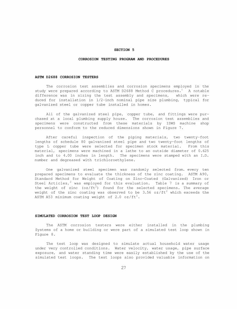
The corrosion test assemblies and corrosion specimens employed in the study were prepared according to ASTM D2688 Method C procedures1 A notable difference was in sizing the test assembly and specimens which were re-duced for installation in 12-inch nominal pipe size plumbing typical for galvanized steel or copper tube installed in homes
All of the galvanized steel pipe copper tube and fittings were pur-chased at a local plumbing supply house The corrosion test assemblies and specimens were constructed from these materials by ISWS machine shop personnel to conform to the reduced dimensions shown in Figure 7
After careful inspection of the piping materials two twenty-foot lengths of schedule 80 galvanized steel pipe and two twenty-foot lengths of type L copper tube were selected for specimen stock material From this material specimens were machined in a lathe to an outside diameter of 0625 inch and to 400 inches in length The specimens were stamped with an ID number and degreased with trichloroethylene
One galvanized steel specimen was randomly selected from every ten prepared specimens to evaluate the thickness of the zinc coating ASTM A90 Standard Method for Weight of Coating on Zinc-Coated (Galvanized) Iron or Steel Articles2 was employed for this evaluation Table 7 is a summary of the weight of zinc (ozft2) found for the selected specimens The average weight of the zinc coating was observed to be 356 ozft2 which exceeds the ASTM A53 minimum coating weight of 20 ozft2
SIMULATED CORROSION TEST LOOP DESIGN
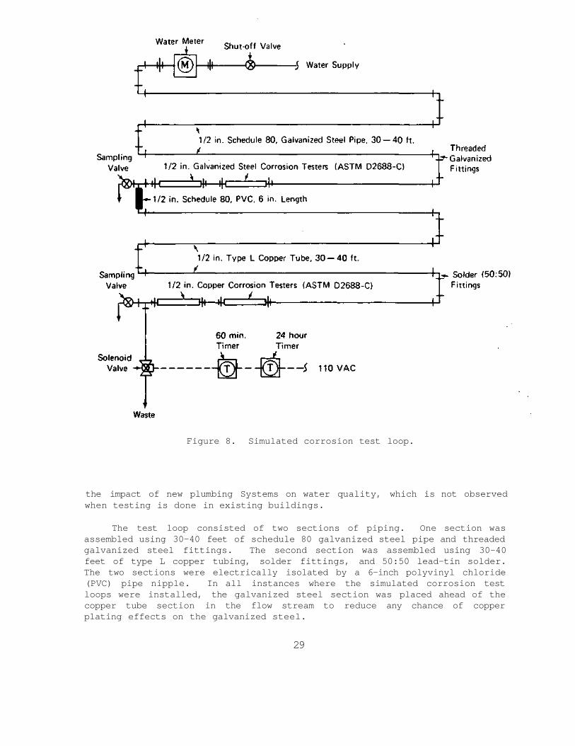
The ASTM corrosion testers were either installed in the plumbing Systems of a home or building or were part of a simulated test loop shown in Figure 8
The test loop was designed to simulate actual household water usage under very controlled conditions Water velocity water usage pipe surface exposure and water standing time were easily established by the use of the simulated test loops The test loops also provided valuable information on
27
Figure 7 Cross section of specimen spacer sleeve and union of assembled corrosion tester
Prepared from 12-inch Schedule 80 galvanized steel pipe 0546 in ID
28
TABLE 7 ZINC COATING Specimen
no
G066 G068 G063 G058 G013 G047 G060
0N INTERIOR Surface area (in2)
686 686 686 686 686 686 686
SURFACE OF Total zinc
(g)
4179 5376 5016 4475 4331 4478 5773
GALVANIZED STEEL SPECIMENS Coating weight
(ozft3)
309 398 371 331 321 332 427
Figure 8 Simulated corrosion test loop
the impact of new plumbing Systems on water quality which is not observed when testing is done in existing buildings
The test loop consisted of two sections of piping One section was assembled using 30-40 feet of schedule 80 galvanized steel pipe and threaded galvanized steel fittings The second section was assembled using 30-40 feet of type L copper tubing solder fittings and 5050 lead-tin solder The two sections were electrically isolated by a 6-inch polyvinyl chloride (PVC) pipe nipple In all instances where the simulated corrosion test loops were installed the galvanized steel section was placed ahead of the copper tube section in the flow stream to reduce any chance of copper plating effects on the galvanized steel
29
Water flow through the test loop was monitored by a positive displace-ment cold water meter Water usage was regulated by an electrically operated solenoid valve controlled by the two timers shown in Figure 8 The 24-hour timer was set to allow the 60-minute timer to operate for 16 hours each day The 60-minute timer was then adjusted to open the solenoid valve every hour for 5-10 minutes Final adjustment of the flow rate was accomplished by use of the shut-off valve
In the loop there was a period of eight hours of constant exposure to standing water which could be regulated to end at a convenient time for sample collection
CORROSI0N TEST SITE INSTALLATIONS
When a long-term corrosion study is undertaken consideration must be given to unforeseen events which could cause the loss of data from any one testing site The chance for this occurring increases when corrosion tests are conducted in the field as compared to controlled laboratory investiga-tions To reduce the risk of data loss corrosion test sites were located where skilled personnel were readily available for the long-term sampling testing and maintenance requirements at each site Therefore a prerequi-site was established that personnel at each testing site have experience in determining pH and chlorine residuals Corrosion test sites were located where ISWS staff licensed water plant operators or environmental science students were available and the sites were easily accessible to these personnel
The water quality of public water supplies has been observed to change within the distribution system3 Corrosion tests at one location in a water supply may not be indicative of corrosion rates at another location Because of this concern corrosion test sites were installed at two locations in four of the water supplies studied A site was located at the water treat-ment plant and another site was located at some distance away in the distrishybution system
Originally the corrosion study considered one test site for each water supply In order to investigate the impact of two piping materials at two separate locations in the distribution System the number of test sites had to be increased from two to four in some of the water supplies The number of test sites were limited to nineteen ten copper and nine galvanized steel systems Water usage and test site locations are summarized in Table 8 A brief description of each test site follows
Sites 301 and 302
Two corrosion test sites were installed in the water treatment building of water supply A (Figure 9) The copper test site (301) and the galvashynized steel test site (302) were located in the existing plumbing system supplying two restrooms Each restroom contained one sink and one toilet The facilities were primarily used by laboratory and operations personnel between 700 am and 500 pm A night operator occasionally used the
30
Two-year period of corrosion study
Figure 9 Corrosion test sites 301 and 302
31
Site no
301 302 303 304 305 306 307 308 309 310 311 312 313 314 315 316 317 318 319
TABLE 8 WATER USAGE
Water supply Plumbing materials
A A A A 3 B B C C C C E E D D F F F F
Copper Galv steel Copper Galv steel Copper Galv steel Copper Copper Galv steel Copper Galv steel Copper Galv steel Copper Galv steel Copper Galv steel Copper Galv steel
AT TEST SITES
Service
Restroom showers Restroom showers Kitchen bathroom Kitchen bathroom Simulated Simulated Total household Simulated Simulated Simulated Simulated Clothes washer Pots amp pans washer Simulated Simulated Simulated Simulated Simulated Simulated
Avg rat
usage e (gpd)
229 229 99 158 201 201 405 341 341 375 375 97 29 167 167 220 220 191 191
facilities Average daily water usage for sites 301 and 302 during the study was 229 gal per day
The galvanized steel test assemblies were installed in a horizontal 12-inch galvanized steel Service line prior to the 12-inch type L copper tubing servicing the restrooms The copper test assemblies were installed in the vertical section of the copper service line Sixteen feet of copper tubing preceded the chrome-plated sample valve at site 301 and 18 feet of galvanized steel pipe preceded the chrome-plated sample valve at site 302 The water meter and water usage was common to both sites Water samples were collected and tested by the water plant laboratory personnel
Sites 303 and 304
Two adjacent houses a mile distant from the water treatment plant in water supply A were selected for the installation of corrosion test assemblies (Figure 10) Site 303 was a typical one-story house with copper plumbing Site 304 was a typical two-story house with galvanized steel plumbing
The houses were used as offices for university personnel therefore water usage was confined to office hours 730 am to 530 pm Monday through Friday Water usage was restricted to hot or cold water needs in kitchens or bathrooms as no laundry facilities were installed in either house The average daily water consumption at site 303 and site 304 was 99 gal per day and 158 gal per day respectively
Samples were collected from a chrome-plated faucet at the kitchen sink Approximately 30 feet of 12-inch piping preceded each sample valve not including the service line from the distribution water main Students in an environmental science program collected the samples and conducted the tests under the supervision of a senior environmental engineer
Figure 10 Corrosion test sites 303 and 304
32
Sites 305 and 306
A simulated corrosion test loop (see previous section) was located in water supply B and installed in the basement of the Water Resources Building housing the Illinois State Water Survey (Figure 11) The location was selected as a control site where ISWS personnel would be available to collect all water samples and make field tests The site was easily accessible for investigating phenomena arising during the study
Site 306 the galvanized steel section of loop was preceded by 65 feet of existing 12-inch schedule 40 galvanized steel pipe Site 305 copper section of loop was separated from the galvanized section by a PVC pipe nipple Each section of the loop was 30 feet in length prior to the respec-tive sampling valves
Water usage was controlled by a timer-regulated solenoid valve and averaged 201 gallons per day during the corrosion study
Site 307
Corrosion test assemblies were installed in the existing copper plumbing of a two-bathroom tri-level home located in water supply B (Figure 12) The home was built in the late 1950s and is located approxi-mately 3-12 miles distant from sites 305 and 306 Site 307 was supplied water from the west treatment plant while sites 305 and 306 were supplied water from the east treatment plant of water supply B
Approximately 25 feet of 34-inch copper tubing preceded the water meter and test assemblies followed by an additional 25 feet of 12-inch copper tube preceding the chrome-plated sampling valve located at the kitchen sink The corrosion specimens were exposed to the total water use of four adults residing in the house The water consumption averaged 405 gallons per day during the corrosion study
Figure 11 Corrosion test sites 305 and 306
33
Figure 12 Corrosion test site 307
The senior author collected all water samples and made all field tests at site 307
Sites 308 and 309
A simulated corrosion test loop was located in water supply C at the water treatment building (Figure 13) Originally the two sites were to employ unsoftened and untreated water directly from a well supplying water to the treatment plant Plumbing complications and space restrictions dur-ing the installation of the test loops caused partially softened and treated water to be employed except during periods where the water softeners were out of service
The galvanized steel section (site 309) was connected directly to gal-vanized steel piping immediately following the water softeners The copper section (site 308) of the test loop followed the galvanized steel section and was separated by a 6-inch length of PVC pipe Both sections contained 35 feet of 12-inch piping Water usage was controlled by the timer-solenoid valve arrangement described in the previous section The water usage averaged 341 gallons per day during the corrosion study
Water samples were collected and field tests were made by the water plant operator who has been licensed to operate both the water and the sewage treatment plant for the state facility
34
Figure 13 Corrosion test sites 308 and 309
Sites 310 and 311
A second simulated corrosion test loop was also located in water supply C and was installed in the maintenance building of the correctional facility (Figure 14) The test loop was directly connected to galvanized steel piping servicing the vehicle wash area which operated eight hours per day The water from the distribution system was considered equilibrated at this location
The service line consisted of approximately 75 feet of 34-inch galvashynized steel pipe Each section of the simulated corrosion test loop galvashynized steel (site 311) and copper (site 310) contained 35 feet of 12-inch pipe
Water usage controlled by the timer-solenoid valve arrangement averaged 375 gallons per day during the study Samples were collected and field tests were made by the same water plant operator responsible for sites 308 and 309
Sites 312 and 313
The corrosion test sites were located in water supply E and were installed in the existing plumbing of a State building housing 200 mentally handicapped children (Figure 15) Two galvanized steel corrosion test assemblies (site 313) were installed in a 40-foot section of 12-inch schedule 40 galvanized steel line servicing a kitchen sink that was used primarily for washing pots and pans An existing chrome-plated valve at the sink was employed for sampling purposes Usage of water at site 313 was confined to the period between 700 am and 500 pm daily and averaged 29
35
Figure 15 Corrosion test sites 312 and 313
36
Figure 14 Corrosion test sites 310 and 311
gallons per day the lowest usage rate of any site observed during the cor-rosion study
At site 312 two copper corrosion test assemblies were installed in a 15-foot section of 12-inch type L copper piping servicing an institutional clothes washer A new chrome-plated valve was installed prior to the clothes washer for sampling purposes Water usage was confined to daytime hours between 700 am and 500 pm and averaged 97 gallons per day during the study
Water samples were collected and field tests were made at both sites by the licensed water plant operator on the staff of the state facility
Sites 314 and 315
A simulated corrosion test loop was located in a water treatment building in water supply D The simulated test loop at this location was vertically oriented due to wall space limitations Figure 16 is a schematic of the piping associated with sites 314 (copper) and 315 (galvanized steel)
Water usage was controlled by the timer-solenoid valve arrangement employed in all simulated test loops and averaged 167 gallons per day during the corrosion study Water samples were collected and field tests were made by the same individual responsible for sites 312 and 313
Sites 316 and 317
A simulated corrosion test loop was installed at the water treatment plant of water supply F (Figure 17) The test loop was connected to a 4-inch cast-iron line supplying wash water to the filters Forty-six feet
Figure 16 Corrosion test sites 314 and 315
37
Figure 17 Corrosion test sites 316 and 317
of 12-inch schedule 40 galvanized steel pipe was installed between the test loop and cast-iron service line The galvanized steel section (site 317) and the copper section (site 316) of the test loop were constructed from 34 feet of 12-inch piping per section
The water usage was controlled by the timer - solenoid valve arrange-ment however during the first two months of operation the timer mechanism failed to operate Three sets of water samples were collected by water plant personnel during this period when the flow was restricted to the flushing of water during the collection of samples Because of timer failure the original set of corrosion specimens were removed and a new set of specimens were installed The corrosion study was reinitiated with ISWS field staff responsible for testing and collecting of samples Water usage averaged 220 gpd after the timer was repaired
Sites 318 and 319
A second simulated corrosion test loop was located in water supply F approximately two miles distant from sites 316 and 317 The test loop was installed in a building of a state mental facility and was connected to a service line supplying water to a closed recirculating heating system (Figure 18) The connection was near the main water supply line and water meter servicing the facility
Water samples were tested and collected by building engineers who proved to be reliable and conscientious in following sampling procedures throughout the study Water usage averaged 191 gpd at sites 318 (copper) and 319 (galvanized steel)
38
Figure 18 Corrosion test sites 318 and 319
REFERENCES
1 ASTM Book of Standards D2688 Method C 31162 (1980)
2 ASTM Standards on Hot-Dip Galvanized Coatings Specification A9032 (1967)
3 Zajecek 0 T Quality Variations Within A Small Water Distribution System Water Resources Research Center U of Mass No 63 (1976)
39
SECTION 6
FIELD METHODS FOR COLLECTING HANDLING AND TESTING OF SAMPLES
SAMPLE COLLECTION PROCEDURES
Standard sampling procedures were established prior to commencing the corrosion study The procedures were needed to guarantee uniformity and control for the collection testing and handling of water samples USEPA-approved methods for sampling water were followed when applicable All responsible personnel were provided written Instructions and were given a personal demonstration of the correct sampling techniques by ISWS field personnel (Appendix D)
Chlorine test kits pH meters and thermometers were provided at all corrosion test sites Chlorine reagents pH buffers sample bottles shipping cartons and ice packs were also supplied as needed ISWS personnel visited each Site at six-week intervals to insure that proper testing and sampling procedures were being followed
Where corrosion test sites were located in homes or buildings water samples were collected frora the cold water tap during early morning hours prior to morning water demands This required that samples be taken between 500 am and 700 am The simulated corrosion test loops were regulated to allow samples to be taken at convenient times for sampling personnel with absolute control of running and standing intervals Water samples were taken from the galvanized steel section of the simulated test loop prior to sampling the copper section to preserve standing conditions in the copper section
At all corrosion test sites water samples were collected from a chrome-plated brass faucet or service tap Screen filters were removed from the faucets prior to sampling The first 50-100 mL of water was collected from the tap for a temperature measurement of the standing sample The next 125 mL of water drawn from the tap was collected in a 125-mL Polyethylene bottle containing acid for use in determining the metal concentrations of the standing water in the test loop
The sampling valve was then opened to allow approximately 12 gpm of water to flow to waste until the water temperature appeared stable and rep-resentative of the distribution water (usually a 4-5 min interval) The temperature of the running sample was recorded and a second 125 mL of water was collected in a Polyethylene bottle containing acid for use in detershymining the metal concentrations of the running water The remaining two
40
Polyethylene sample bottles 125-mL and 500-mL and a glass vial for TOC analyses were filled with the running water from the tap
The sample bottles were capped and labelled by date time site number and sample number Chlorine and pH measurements were made on the running water after the samples had been collected The pH value chlorine concenshytrations temperatures and meter reading were then recorded on a prepared form for enclosure with the sample bottles
SAMPLE PRESERVATION AND HANDLING PROCEDURES
The chemical concentrations of the constituents in the drinking water which could not be reliably preserved during shipment of the samples to the analytical laboratory were determined at each corrosion test site This was considered essential for pH measurements since reliable pH values were necessary for meaningful evaluation of the data Dissolved oxygen free chlorine residual and total chlorine residual concentrations were also made at the test site because sample preservation methods were not available for these constituents
The 125-mL water samples collected for running and standing metal conshycentrations were preserved by addition of 25 mL of 11 HNO3 prepared from AA grade nitric acid The 125-mL water sample collected for total phosphate analyses was preserved with 10 mL of concentrated reagent grade sulfuric acid The sulfuric-acid-preserved sample was also used when nitrate concenshytrations were rechecked in the laboratory
Styrofoam insulated cartons were used to ship water samples to the laboratory Two ice packs were placed in each carton with the five water samples prior to shipment Water samples from corrosion test sites 301 302 303 304 308 309 310 311 318 and 319 were shipped by one-day express bull delivery Services Samples from the remaining test sites were delivered directly to the laboratory by sampling personnel The water samples were refrigerated until time of shipment if delays were experienced
Upon receipt of the water samples in the laboratory the alkalinity silica orthophosphate polyphosphate TOC and total dissolved solids conshycentrations were determined Early in the study laboratory personnel were observed delaying analyses until a minimum number of samples were available Water samples for trace metal determinations were allowed to accumulate in the lab for trace metal determinations since the samples were acid-pre-served The trace metal concentrations were found to be stable in these samples after a year in storage
FIELD TEST METHODS
Free available chlorine residual total (free and combined) chlorine residual pH and dissolved oxygen concentrations were determined at each test site when water samples were collected The field test methods for these constituents are briefly described in the following sections
41
Chlorine Residuals
Precise measurements of chlorine residuals were not considered as essential as employing a simple but reasonably accurate chlorine procedure which could be easily and uhiformly applied by field personnel A field test kit method meeting these criteria (LaMotte Chemical DPD Chlorine Test Kit Model LP-26) was selected for use during the corrosion study Free and total chlorine residuals were determined using the test kit based on the DPD (diethyl-p-phenylene diamine) method developed by Palin1 DPD reagents were stable when supplied in tablet form and sealed in foil packets The color comparator used color standards representing 02 04 06 08 10 15 20 and 30 mgL Cl2 The sample Instructions for determining free chlorine and total chlorine residuals using the test kit are described in Appendix D
pH
Reasonably accurate pH measurements were required for the corrosion study since pH is a major influence on the corrosivity of water Color comparator test kits for pH measurement were not considered sufficiently accurate The electrometric method2 using a glass electrode for determining pH was selected for use at all corrosion test sites Where pH meters were not available to sampling personnel a pH meter and pH buffers were pro-vided ISWS field staff checked the pH meter calibration and electrode response every six weeks Glass andor reference electrodes were replaced when electrode response was unsatisfactory Commercial pH 70 and pH 90 buffer solutions (plusmn001 pH unit) were used for standardizing the pH meters
Portable battery-operated pH meters were employed at all test sites except sites 301 and 302 where a line-operated pH meter was available near the sampling point After calibration of the pH meter grab samples of the running water were taken in succession until a stable pH reading was obtained pH and temperature values were reported for every water sample submitted to the laboratory except when a pH meter was not functioning properly
Dissolved Oxygen
ISWS field staff determined the dissolved oxygen concentrations of the running water samples at six-week intervals The azide modification of the Winkler method3 was adapted to a portable field kit for this purpose A 300-mL volume of the running sample was collected through rubber tubing and trapped in a narrow-mouth glass-stoppered B0D bottle Reagents were added to the bottle mixed and a 203-mL aliquot was titrated with standard thio-sulfate as outlined in the procedure Dissolved oxygen concentrations were reported to the nearest 01 mgL
Temperature
General purpose mercury-in-glass thermometers were used for determining the temperatures of the running and standing water samples collected at each test site A bulk purchase of thermometers was made prior to the corrosion
42
study and the accuracy of the thermometers was checked with the ice point and boiling point of water Thermometers more than 1degC in error were dis-carded
The temperature range of the thermometers was -20degC to +110degC with a 1degC resolution The temperature was determined by immersing the thermometer to the 76-mm mark in the water sample Temperature values were reported to the nearest 05degC
REFERENCES
1 Palin A T Methods for the Determination in Water of Free and Combined Chlorine Chlorine Dioxide Chlorite Bromine Iodine and Ozone Using Diethyl-p-phenylenediamine (DPD) J Inst Water Eng 2537 (1967)
2 Standard Methods for the Examination of Water and Wastewater 14th Edition APHA-AWWA-WPCF Part 422B (1975)
3 Standard Methods for the Examination of Water and Wastewater 14th Edition APHA-AWWA-WPCF Part 424 (1975)
43
SECTION 7
LABORATORY ANALYTICAL METHODS
TRACE METAL AND MAJOR CATION DETERMINATIONS
Trace metal (Fe Zn Mn Cu Pb Cd) and major cation (Ca Mg Na K) determinations were performed by the Analytical Chemistry Unit of the State Water Survey on a contract basis They were performed by either conven-tional flame atomic absorption spectroscopy (AAS) or by flameless graphite furnace atomic absorption spectroscopy (GFAAS)
A Perkin-Elmer model 380 AA spectrophotometer was used for the flame atomic absorption analyses when the concentrations were high enough to per-mit its use The instrument was calibrated using the built-in procedure which employed a blank and two standards to define the analytical curve and provide a basis for direct concentration readout Additional check stanshydards were inserted in the runs to monitor linearity of response Samples with concentrations beyond the linear working range were diluted A releasing agent consisting of a 1 lanthanum solution (in HCl) was used for calcium and magnesium determinations An ionization suppressant consisting of a 1 cesium chloride solution was employed in the sodium and potassium determinations
An Instrumentation Laboratory model 151 AA spectrophotometer with a model 655 graphite furnace and model 254 (FASTAC) automatic sampler was used for the bulk of the flameless AA analyses Late in the project an IL Video 22 AA spectrophotometer supplanted the model 151 Concentrations were cal-culated from calibration curves of peak heights versus standard concentrashytions The Cd determinations utilized deuterium arc background correction No matrix modifiers were used for any of these metals
All of the metal analyses were done on solutions preserved with 25 mL of 50 vv ultrapure nitric acid in the 125-mL sample bottle The amount of time that elapsed before analysis was variable but was within the latest EPA recommended guideline of six months1
MAJOR ANION DETERMINATIONS
Sulfate nitrate and chloride were determined using a Dionex model 12 Ion Chromatograph with an autosampler and a conductivity detector Samples were unpreserved and filtered through a 045-um pore-size cellulose acetate
44
membrane using a glass vacuum filtration apparatus Originally concentra-tions were determined from calibration curves based on peak heights measured from a chart recorder output Later a locally developed software system on an Apple II Computer was used to record peak heights and calculate calibrashytion data The extreme range of concentration of sulfate and chloride caused many problems of peak overlap Also large dilutions were necessary to bring the sample concentrations down to the normal operating range of this instrument which was normally one appropriate for rainwater analysis
Most of the IC analyses were performed within the 28-day suggested holding limit for sulfate and chloride However few analyses were done within the 48-hour limit suggested for nitrate A major problem encountered was that by the time the analytical results were returned to project personnel the suggested holding times were usually greatly exceeded The chloride levels were probably still stable but repeat determinations of nitrate performed on the unpreserved samples indicated that the nitrate concentrations in many of those samples were unstable The relatively poor precision of all sulfate methods attempted did not enable any firm conclu-sions to be drawn concerning sulfate stability in the samples
Manual spectrophotometric methods were used to determine the concentrashytions of orthophosphate and of total inorganic phosphate The absorbances after color development were measured on either a Perkin-Elmer Lambda 3 or Beckman model DBG spectrophotometer in almost all cases A Beckman DU spectrophotometer was employed for the remaining samples
Unpreserved 045-μm filtered samples were used for orthophosphate deshyterminations The total inorganic phosphate analyses actually acid hydrolyzable phosphate analyses were done on samples preserved in the field with 10 mL analytical reagent grade sulfuric acid The analytical method used most closely corresponds to that described by Robertson2 and ASTM procedures3
Considerable problems were encountered in getting orthophosphate analyses performed in a short time after sample receipt The problem is critical because at one time or another during the project inorganic poly-phosphate treatment chemicals were used at sites 301 302 303 304 312 313 314 and 315 Polyphosphates hydrolyze upon standing Converting to the orthophosphate form Thus although the total inorganic phosphate concenshytrations should remain stable the orthophosphate fraction will continually develop a high bias over time
The error introduced by delayed analyses was investigated in a special study reported in a later section After approximately November 14 1983 additional efforts were made to speed orthophosphate analyses and samples were kept refrigerated at 4degC until analyzed to slow hydrolysis An examina-tion of the analytical and collection records revealed that delays of two to four weeks were typical and sometimes reached eight weeks The orthophosshyphate levels reported for all sites containing polyphosphates except per-haps 312 and 313 must be considered to be significantly in error with a variable positive bias
45
MISCELLANEOUS ANALYSES
Silica analyses were originally performed using an undocumented molyb-denum blue procedure similar in many respects to that recommended by ASTM4 During June and July of 1983 the Performance of the method was evaluated in detail using USGS Standard Reference Water Samples and commercially prepared stock standard solutions The method had been previously found to be very time sensitive so that only a small number of samples could be run per analysis batch Further the Performance was found to be somewhat inconsis-tent in the hands of our analysts normally yielding high bias Therefore from July 12 1983 onwards all silica analyses were done using the manual ascorbic acid reductionmolybdenum blue procedure of the US Geological Survey5
Total alkalinity titrations were initially performed on the filtered unpreserved samples by titrating with standardized 002 N sulfuric acid to an endpoint of pH 450 In late January 1983 the alkalinity method was changed to a Gran plot titration with 002 N HCl titrant as described by Kramer6 This change not only reduced the time required for each analysis but greatly improved the accuracy of the determinations Titration equiva-lence points were computed by a Hewlett-Packard HP-34C calculator program
The total dissolved solids (TDS) analyses were done by evaporating a 100 mL aliquot of filtered unpreserved sample to dryness on a steam bath in preweighed glass dishes and finally drying completely at 105degC in an oven The samples were cooled to room temperature in a desiccator and were then weighed in a 4-place (01 mg) mechanical or electronic analytical balance
Total Organic Carbon analyses were performed along the procedural lines given by Barcelona7 for the nonvolatile fraction (NVOC) The instrument used was an Oceanographic International Model 524 T0C Analyzer with direct injection module purging and glass ampule scaling units and an infrared detector Calibrations were calculated relative to potassium hydrogen phthalate standards
Analytical rechecks of chloride values were done with silver nitrate titrations using first an adsorption indicator endpoint (Standard Methods 408A)8 and later a Potentiometric endpoint sensed by a double junction reference electrode (Corning 476067) and Ag2S membrane electrode (Orion 94-16) pair The Potentiometrie titrations were done in the presence of 1 mL concentrated HNO3 which served to limit silver ion adsorption and an ionic medium buffer Titrations were carried out to a set potential endshypoint determined at the start of the analytical session by averaging observed potential readings from replicate titrations of chloride standard solutions
Sulfate repeat determinations were done using barium Perchlorate titrashytion with Thorin indicator following methods of Haartz et al9 Cook and Miles10 and USGS5
Nitrate rechecks were done on both unpreserved and sulfuric acid pre-served samples by the chromotropic acid spectrophotometric method7
46
The acid-preserved samples yielded the most consistent results in comparison with the original analyses although significantly different concentrations from the ion chromatograph values were found for many samples
QUALITY CONTROL PROCEDURES
Periodically trace metal reference standards were received from the USEPA These glass ampule sets were turned directly over to the Analytical Chemistry Laboratory Unit for analysis and the results were sent directly to the USEPA project officer We are aware of no problems that were indi-cated in these quality control checks
Relatively late in the project Standard Reference Water Samples for both trace metals and mineral constituents were obtained from the US Geological Survey These samples were immediately applied to use as intershynal QC samples in our analytical runs and were further used as blind unknowns submitted along with other project samples Additional USEPA Environmental Monitoring and Support Laboratory quality assurance sample ampules were obtained and prepared to evaluate residual chlorine filterable residue mineral trace metal and nutrient analyses The blind unknowns indicated the expected analytical accuracy for all constituents (except orthophosphate and free chlorine residual) to be on the order of plusmn5-10 relative Every tenth sample received was split and submitted as duplicate samples to monitor the adequacy of the precision of the analyses
Analytical data were periodically reviewed by the principal investiga-tors and questionable data were flagged for additional scrutiny based on previous behavior of the water Systems under investigation When the Comshyputer data base was completed an interface program was developed to pass all of the analytical data through a modified version of the WATSPEC aqueous chemical equilibria program In addition to Computing ion balance errors after considering the aqueous chemical speciation in the samples incompati-bilities between pH and alkalinity were tested Samples failing the ion balance test by more than plusmn10 were reanalyzed for appropriate anionic or cationic constituents Samples with incompatible pH and alkalinity values and samples with major chemical parameters not analyzed were deleted from the data base in their entirety Figure 19 shows the final distribution of ion balance errors
A total of 890 samples were collected during the course of the study Of these 35 (4) samples were reanalyzed by at least one method for chloride sulfate and nitrate before ion balances were performed Following the ion balance computations 38 samples were reanalyzed for the same three constituents Fifteen samples were reanalyzed for TDS seven for alkalinshyity and seven for total inorganic phosphate Records are not readily available for the number of major metals reanalyzed but the analytical Problems were largely confined to the anionic constituents Most samples having metal concentrations in excess of the MCL were reanalyzed as a matter of course Approximately 100 additional samples were reanalyzed for zinc copper andor lead
47
Figure 19 Distribution frequency of ion balance errors
STUDY OF THE REVERSION OF POLYPHOSPHATE TO ORTHOPHOSPHATE
In order to ascertain whether or not significant bias was introduced into the orthophosphate and hydrolyzable phosphate determinations by the long waiting times before sample analysis a laboratory study was initiated in November 1983 A total of eighteen 500-mL samples were taken at both site 312313 and site 314315 on November 14 An acid-preserved sample was also taken at each location The samples were immediately refrigerated and returned to the laboratory for analysis within two hours of collection
At the laboratory half of the samples from each site were separated and were kept refrigerated at 4degC in a cold room until analyzed The other half were maintained at the ambient laboratory temperature 20-25degC
The first day (T = 0) triplicate aliquots were taken from the acid-preserved and unpreserved samples from each site and analyses were performed for orthophosphate and acid hydrolyzable phosphate The results are summarized in Table 9 The behavior of the polyphosphate at site 314315 is already considerably different from its behavior farther along in the same system (site 312313) While at site 312313 the acid hydrolyzable phosphate (AHP) is the same in the acid-preserved and nonpreserved portions a considerable difference is apparent for those fractions at site 314315
48
TABLE 9 FIRST-DAY ANALYTICAL DATA FOR THE PHOSPHATE REVERSION STUDY (mg PO4L)
Refrigerated and room temperature unpreserved samples were then analyzed in triplicate after 1 2 3 7 14 21 28 and 44 days The data are plotted in Figures 20 through 23 with the error bars indicating plus or minus one standard deviation As can be seen in Figures 20 and 21 the orthophosphate and AHP concentrations remained essentially identical throughout the test period although some very slow reversion might be indi-cated after approximately 20 days (not statistically significant at the 95 level)
At site 314315 the polyphosphate behavior is considerably different Rapid reversion of polyphosphate to orthophosphate is evident in Figure 22 Refrigeration slowed the reversion rate considerably but the concentration of orthophosphate still doubled within seven days Interestingly the AHP fraction also increased tremendously in the first week One explanation for the observation oould be the presence of an organic phosphate fraction which might have been formed by reaction of the inorganic polyphosphate treatment chemical with naturally occurring organic material This form may have been rapidly hydrolyzed upon acid addition invalidating the implicit assumption that the total phosphate in the sample was simply the sum of the orthophosphate plus the polyphosphate from the treatment chemicals It is not at all clear however why the immediate addition of sulfuric acid upon collection results in higher AHP values
The differences between the refrigerated and nonrefrigerated samples from Site 314315 were significant at the 95 level (t-test) Similarly the differences between the AHP function and the orthophosphate were also significant Figures 24 and 25 show the behavior of reference standards analyzed in conjunction with the sample stability test They did not vary at the 95 confidence level indicating that the analytical procedures remained in control throughout the study
49
Site
312313
314315
Al iquot
1 2 3
1 2 3
Acid Ortho-
11
1 1
11
11
1 1
11
-preserved PO4 AH-PO4
267 259 267
643 648 648
Unpreserved 0rtho-PO4
1 70 1 64 1 70
033 025 030
AH-PO4
261 261 259
200 1 97 1 97
Figure 20 The effect of refrigeration and time on the orthophosphate concentration in samples from sites 312313
Error bars represent plusmn1 standard deviation
50
Figure 21 The effect of refrigeration and time on the acid hydrolyzable phosphate concentration in
samples from sites 312313 Error bars represent plusmn1 standard deviation
51
Figure 22 The effect of refrigeration and time on the orthophosphate concentration in samples from sites 314315
Error bars represent plusmn1 standard deviation
52
Figure 23 The effect of refrigeration and time on the acid hydrolyzable phosphate concentration in
samples from sites 314315 Error bars represent plusmn1 standard deviation
53
Figure 24 Analyses of USEPA quality control standards for ortho-phosphate to verify analytical Performance during the stability study
54
Figure 25 Analyses of USEPA quality control standards for acid hydrolyzable phosphate to check analytical Performance during
the stability study Standards contained only orthophosphate
55
The conclusions from this study are the following
1 Orthophosphate and acid hydrolyzable phosphate data from sites 312 and 313 are reasonable regardless of time delays before sample analysis
2 Orthophosphate data from sites 314 and 315 are probably in large error for almost all of the project period The data are somewhat more reliable after December 1983 but delays of several days were still frequent No simple correction can be applied to these data
3 All of the inorganic phosphate treatment dosage may not be accounted for by the analytical pro-cedures used on this project
4 No statement can be made about the reliability of orthophosphate data from sites 301 302 303 or 304 during the periods when polyphosphates were added to that system
REFERENCES
1 Methods of Chemical Analysis of Water and Wastes US Environmental Protection Agency Environmental Monitoring and Support Laboratory EPA 6004-79-020 (Mar 1979)
2 Robertson R S Rapid Method for Estimation of Total Phosphate in Water Jour AWWA 524483 (1960)
3 Standard Test Methods for Phosphorus in Water D515-78 ASTM Book of Standards Part 31 Water (1981)
4 Standard Test Methods for Silica in Water D859-80 ASTM Book of Standards Part 31 Water (1981)
5 Skougstad M W et al Methods for Analysis of Inorganic Substances in Water and Fluvial Sediments US Geological Survey Open File Report 78-679 (1978)
6 Kramer J R Precise Determinations of Low Alkalinities Using the Modified Gran Analysis An Inexpensive Field Procedure Environmental Geochemistry Report 19801 McMaster University Hamilton Ontario Canada (1982)
7 Barcelona M J T0C Determinations in Ground Water Ground Water 22118 (1984)
56
57
8 Standard Methods for the Examination of Water and Wastewater 14th Edition APHA-AWWA-WPCF (1975)
9 Haartz J C et al Critical Parameters in the Barium PerchlorateThorin Titration of Sulfate Anal Chem 51132293 (1979)
10 Cook J M and Miles D L Methods for the Chemical Analysis of Groundwater Institute of Geological Sciences Natural Environmental Research Council Report 805 HMSO London (1980)
SECTION 8
LABORATORY CORROSION INVESTIGATIONS
DIFFERENTIATION OF DISSOLVED AND PARTICULATE PRODUCTS
An investigation into the nature of the metal content in the water at several sites was called for because of several observations including (1) metal concentrations of samples were inconsistent (2) particulate matter was accumulating on filter membranes and (3) metal concentrations of samples were exceeding their predicted solubility The investigation was confined to sites 305 306 312 313 314 and 315 where a State Water Survey chemist could take the samples and perform the filtration activities at the time of collection
The published reports of many previous investigations of metal filtrashytion methodologies were examined before the procedure described here was implemented This procedure follows many of the previous published sugges-tions1-5 Although this procedure was designed to minimize adsorption loss to the filter and apparatus some small loss (less than 5-10) was probably inevitable The procedure described below for sites 305 and 306 is repre-sentative of the procedure for all sites where filtered samples were taken
1 First a 04 μm Nuclepore(R) polycarbonate membrane filter was placed with plastic-tipped forceps into an all-plastic (polycarbonate) 047-mm-diameter in-line filtration assem-bly
2 The assembled filtration apparatus was rinsed with approxi-mately 500 mL of AR grade 11 (vv) nitric acid by drawing the acid through the line (Tygon(R) tubing) by a peristaltic pump The filtration apparatus and tubing were then rinsed by approximately one liter of double-distilled deionized water
3 Immediately the first 125 mL of water from the galvanized pipe loop were collected directly in a 125 mL standard LPE sample bottle to represent the standing unfiltered sample
4 A 500 mL high-density linear Polyethylene (LPE) sample bottle was rinsed with approximately 5 mL of sample withdrawn from the galvanized test loop The rinse water was discarded and the bottle was rinsed with a second 5 mL portion of sample water
58
5 The next 500 mL of sample water were collected in the rinsed LPE bottle
6 Immediately the first 350-375 mL of sample were pumped to waste through the filtration assembly The final 125 mL were collected in a standard 125 mL LPE sample bottle containing the nitric acid sample preservative
7 The used membrane filter was discarded and the filtration assembly was briefly rinsed before a new filter was installed The filtration assembly and a new sample bottle collection were then rinsed as described in steps 1-2 and steps 3-6 were followed for the collection of standing samples from the copper test loops
3 To collect running samples the copper loop tap was opened and the water was allowed to flow for 10 minutes During this time the filter membrane was replaced and the apparatus was acid-washed and rinsed as before
9 A new 500 mL LPE bottle was rinsed as described previously and both filtered and unfiltered 125 mL samples were collected as given in steps 3~6
10 The copper loop tap was closed and the galvanized loop was flushed for 10 minutes After replacing the filter cleaning the filtration assembly and rinsing a 500 mL collection bottle 125 mL filtered and nonfiltered running samples were collected
At sites 312 and 313 only running samples were filtered At sites 314 and 315 two 125 mL standing samples were taken before the filtered standing samples Running samples were also filtered at these two sites
At the time these plans were devised there was not an awareness of the contribution to the observed metal levels by the sampling taps Thus some of the results of this investigation are ambiguous Presumably in the absence of a contribution by the sampling tap the metal levels would be constant until the mixing zone between standing and freshly flowing water would be encountered Thus the filtered third aliquot of 500 mL from sites 314 and 315 was originally assumed to represent the same chemical concentra-tions as would be found in the first two 125 mL portions
At sites 305 and 306 there was little if any evidence for particulate metal species (see Tables 10 and 11) With the exception of the initial sampling episode (21683) only a few scattered pairs of analyses would appear to be in any way outside the bounds of analytical precision or pos-sible adsorption loss during filtration The large differences between filtered and unfiltered copper at site 306 might be attributable to contami-nation from the chrome-plated brass sampling tap rather than to the presence of particulate copper species The cause cannot be determined because the unfiltered standing sample comprised the initial 125 mL of water
59
TABLE 10 COMPARISON OF SOME FILTERED AND UNFILTERED STANDING TRACE METAL CONCENTRATIONS FOR SITE 305 (COPPER PIPE LOOP)
UF = unfiltered F = filtered ∆C = UF minus F all in mgL
TABLE 11 COMPARISON OF SOME FILTERED AND UNFILTERED STANDING TRACE METAL CONCENTRATIONS FOR SITE 306 (GALVANIZED PIPE LOOP)
UF = unfiltered F = filtered ∆C = UF minus F all in mgL
sampled which was in more prolonged contact with the faucet Also because no copper pipe was in the building line to this sampling point some of the higher copper values are puzzling (if the tap is not the cause) Further evidence for faucet contamination will be presented in a later section
Tables 12 and 13 show the data from some running samples from sites 312 and 313 that were also filtered by the procedure described The data show no significant sloughing-off of corrosion products or the presence of col-loidal or suspended particulates in the source water at these sites The consistency of the data also indicates that the filtration methodology resulted in minimizing the trace metal adsorption losses to the filter mem-brane tubing or filter support
60
21683 3883 14683 141483 142183 5383 52483 61383 62283 62783 71283
UF
045 005 005 008 006 005 005 005 015 005 009
Fe F
lt004 lt003 lt003 lt003 004 lt005 lt006 lt006 lt006 lt007 lt007
∆C
gto41 gt002 gt002 gt005 002 ge001 ----
gt009 --
gt002
UF
062 012 01 1 016 015 014 015 015 013 009 011
Cu F
0 16 0 10 007 0 10 012 009 012 011 008 004 008
∆C
0148 002 004 006 003 005 003 004 005 005 003
UF
0 18 002 003 007 004 012 003 005 008 002 0014
Zn F
002 002 002 003 004 002 002 007 001 004 002
∆C
016 000 001 004 000 010 001
-002 007
-002 002
UF
0071 0005 0006 0018 0010 0010 0005 0005 0021 0009 0016
Pb F
0006 0003 0004 0007 0005 0003 0002 0003 0004 0004 0002
∆C
0065 0002 0002 0011 0006 0007 0003 0002 0017 0005 0014
21683 3883 4683 41483 42183 5383 52483 61383 62283 62783 71283
UF
008 005 005 014 028 012 015 007 017 023 011
Fe F
004 004 lt003 010 018 010 lt006 lt006 lt006 lt007 lt007
∆C
004 001
gt002 004 010 002 gt009 gt001 gt011 gt016 gt004
UF
006 003 006 002 029 002 006 003 006 017 003
Cu F
002 001 001 002 006 003 003 001 lt001 lt001 001
∆C
004 002 005 000 023 -001 003 002 gt005 gto 16 002
UF
013 010 010 066
- 067 048 027 017 037 025 015
Zn F
012 009 009 085 071 051 023 020 011 015 009
∆C
001 001 001 -019 -004 -003 004 -003 026 -010 006
UF
0003 0005 0005 0005 0017 0002 0005 0001 0003 0012 0002
Pb F
0002 0001 0001 0007 0012 0003 0005 0002 0001 0001 0001
∆C
0001 0004 0004 -0003 0005 -0001 0000 -0001 0002 0011 0001
TABLE 12 COMPARISON OF MAJOR METAL CONSTITUENTS IN FILTERED AND UNFILTERED RUNNING WATER SAMPLES FROM SITES 312 AND 313
UF = Unfiltered F = filtered concentrations are in mgL
TABLE 13 COMPARISON OF SEVERAL TRACE METALS IN FILTERED AND UNFILTERED RUNNING WATER SAMPLES FROM SITES 312 AND 313
61
Date
21783 42883 62883 82583
21783 42883 62883 82583
Ca UF
12 17 14 14
12 13 14 13
F
12 1b 14 13
12 13 13 13
Mg UF F
Site 312
56 57 79 73 70 69 62 61
Site 313
57 60 57 57 67 67 58 59
Na UF
310 295 296 288
294 303 298 286
F
308 313 298 235
288 300 296 298
K UF
1 4 1 5 1 4 1 2
1 1 1 6 1 5 1 2
F
1 4 1 8 1 4 1 2
1 2 1 6 1 4 1 2
Date
21783 42883 62883 82583
21783 42883 62883 82583
Zn UF
lt001 lt001 001 001
009 003 005 005
F
lt001 lt001 001
lt001
031 003 008 005
Fe UF F
Site 312
016 009 008 010 009 007
lt006 lt006
Site 313
009 005 018 009 009 008 006 006
UF
004 005 004 003
002 002 002 002
Cu F
003 003 004 003
002 002 002 002
Pb UF
0003 0003 0002 0001
0002 0002 0001 0001
F
0002 0003 0001 0001
0003 0001 0001 0001
UF = Unfiltered F = filtered concentrations are in mgL
Tables 14 and 15 show similar data from filtered and unfiltered running samples from sites 314 and 315 Once again perhaps with the exception of iron the trace metals and major constituents were apparently present as dissolved species The observations at these four sites are consistent with the behavior of the polyphosphate treatment chemical as a solubilizing and sequestering agent for a variety of metals The large amount of particulate iron-containing material observed on filter membranes when unpreserved samples were processed at the laboratory is almost certainly the result of air oxidation possibly photochemical from ambient light and longer contact with the chlorine residual in the water The polyphosphate chemical was effective in sequestering reduced iron (ferrous iron) but after prolonged exposure to strong oxidizing conditions some of the iron became oxidized and precipitated from solution
Because filtrations were performed at only six sites and water charac-teristics at other locations were considerably different contribution of particulates to high metal levels in other samples cannot be ruled out
FIELD INVESTIGATIONS OF CONTAMINATION FROM SAMPLING VALVES
Originally standing filtered and unfiltered samples were to be taken at sites 314 and 315 to test for contributions from unprecipitated or non-adherent solid material to complement the running samples described in the previous section There was also considerable concern by this time that the faucets were contributing copper and zinc to the samples The concern arose
TABLE 11 COMPARISON OF MAJOR METAL CONSTITUENTS IN FILTERED AND UNFILTERED RUNNING WATER SAMPLES FROM SITES 314 AND 315
UF raquo Unfiltered F = filtered concentrations are in mgL
62
Date
21983 22483 42883 62883 82583
21783 22483 42883 62883 82583
Ca UF
69 118 58 35 77
69 116 58 38 76
F
64 118 59 34 76
63 115 63 45 77
UF
33 50 27 21 33
33 50 28 22 33
Mg t F
Site 314
31 51 31 21 33
Site 315
31 50 30 25 33
Na UF
164 168 198 198 171
164 169 182 198 169
F
178 168 194 199 171
180 168 180 197 170
K UF
33 35 34 33 34
33 35 36 32 33
F
34 36 36 32 34
34 35 36 33 33
TABLE 15 COMPARISON OF SEVERAL TRACE METALS IN FILTERED AND UNFILTERED RUNNING WATER SAMPLES FROM SITES 314 AND 315
Date
21733 22433 42883 62833 82583
21783 22483 42883 62883 82583
Zn UF
003 005 003 006 002
002 006 005 009 004
F
004 005 006 003 002
003 006 003 005 004
F UF
093 148 056 089 1 06
095 1 47 054 1 44 1 07
e F
Site
0 19 083 039 027 046
Site
020 059 037 054 1 06
314
315
Cu UF
001 001
lt001 001
lt001
lt001 lt001 lt001 001
lt001
F
001 001
lt001 lt001 lt0 01
lt001 lt001 lt001 001 lt001
Pb UF
0001 0001 0001 0032 0012
0002 0004 0008 0003 0001
F
0001 0001 0001 0001 0001
0001 0002 0002 0007 0002
UF = Unfiltered F = filtered concentrations are in mgL
from observations of the large number of standing samples taken from the galvanized loop that showed copper levels of at least a similar concentra-tion to those found for running samples through the copper loop and the large number of standing zinc concentrations in the copper loop that exceeded the running zinc concentrations in the galvanized loop
To test the hypothesis that the chrome-plated brass sampling valves contributed to the metal content of samples two successive 125-mL portions of sample followed by a 500-mL sample were taken at each site The first two were unfiltered The first sample was generally comparable to the standing samples contained in the project data base The third sample was filtered in the manner described previously
The results of these samplings for some major metals as well as trace metals are shown in Table 16 The clear decrease in the trace metal con-centration of successive samples is convincing evidence that the faucets made a significant contribution to the metal content of the solution The low value of the third sample compared to the first two samples cannot be clearly attributed to the presence of particulate material as had been previously thought before the faucet contamination was discovered
There are some particularly interesting trends in the trace metal data If the high zinc levels observed upon standing are presumed to come from the faucet during sampling then the difference between the first and third sample should be approximately the same for both the galvanized pipe system and the copper system This hypothesis seems to be supported by the data
63
TABLE 16 SUCCESSIVE STANDING SAMPLE PORTIONS FROM SITES 314 AND 315
Date
22183 M2833 62883 82583
22183 M2883 62883 82583
Date
22483 12883 62883 82583
22183 12883 62883 82583
Site
311 311 311 311
315 315 315 315
Site
314 314 314 314
315 315 315 315
Calcium 1
73 71 106 77
73 76 107 76
1
072 013 200 1 60
136 201 225 175
2
72 71 107 76
72 71 106 76
Iron 2
036 021 168 060
1 06 038 1 18 298
3
72 73 106 76
71 76 107 77
0 0 0 0
0 0 0 0
3
16 17 38 51
21 23 18 10
Mag 1
31 36 15 34
34 36 45 34
nesium 2 3
31 35 15 31
34 35 11 31
1
025 028 037 034
001 lt001 lt001 001
33 35 11 34
33 35 15 3t
1
171 167 167 190
173 17t 162 137
Copper
bull
2
0 0 0 0
0 lt0 lt0 0
10 09 15 09
02 01 01 01
Sodium 2
172 169 165 136
173 165 161 185
3
007 006 006 005
lt001 lt001 lt001 lt001
3
172 177 16t 187
170 163 163 186
0 0 0 0
0 0 0 0
3 3 3 3
3 3 3 3
1
277 086 085 070
089 19t 018 206
Potassium 1 2
2 32
5 35
7 37
6 35
1 32
5 35
6 36
6 36
Lead 2
0037 0035 0015 0007
0061 0019 0008 0037
3
31 35 36 36
32 37 37 36
3
0005 0015 0007 0005
0007 0008 0002 0002
1
022 013 028 027
1 22 135 296 1 47
Z ine 2
010 0 16 023 0 10
1 21 123 288 1 60
Manganese 1
009 009 022 013
010 009 021 0 17
2
008 009 023 011
0 10 008 024 010
3
007 008 015 010
104 117 264 123
3
008 008 018 009
009 008 021 009
Concentrations are in mgL The third portion (3) was filtered through a 04-μM polycarbonate merabrane Portions 1 and 2 were 125 mL portion 3 was 500 mL
Many researchers have been concerned over potentially dangerous lead leaching from the zinc coating on the galvanized pipe High initial lead levels observed at both the copper and galvanized sites dropped extremely rapidly to only several parts per billion by the third aliquot of sample This indicates not only that there is no important contribution from the galvanizing layer after this length of time (nothing can be said about the earlier samples throughout the project) but that there also is not much of a lead contribution from the solder in the copper loop These conclusions can be justified only for these two sites without further investigation
The trend of the running zinc and lead concentrat ions at the copper loop are somewhat different After about 9 or 10 months of operation the lead levels (with three exceptions) tended to stay below about 001 mgL That possibly reflects the length of time that is necessary to build a passivating coating on the solder or to remove readily-leachable lead from the sampling taps The zinc concentrations continued to be highly variable throughout the project This could possibly indicate that some zinc can still be easily leached from the sampling taps with very Short contact times via either a solubility or dezincification mechanism
At sites 305 and 306 the same problem of possible faucet contamination was studied with a similar but slightly different approach At site 306 a new sampling tap of the same general type as thqse employed at the other
64
sites was installed before the galvanized pipe loop (sample valve x in Figure 11) This was primarily intended to monitor the levels of zinc copper iron and lead going into the corrosion test loop system A small new galvanized T fitting was also installed to enable the chrome-plated tap to be fitted into the source pipe line
Initially only a Single 125 mL standing sample was taken at this loca-tion However after 97 days of operation three successive 125 mL unfil-tered samples were taken and this procedure continued through the end of the operation at this site After 130 days (July 15 1983) the chrome-plated brass faucet was replaced with one of low density linear Polyshyethylene (Nalgene(R)) The data from this special study are given in Table 17
The Information in Table 17 shows clearly that the chrome-plated sampling tap contributed substantial amounts of lead and zinc and somewhat lesser amounts of copper and iron to the standing samples The contamina-tion decreased with time but still remained considerable after more than five months The elevated zinc values for the first 125-mL samples with the Polyethylene faucet represent a contribution from the relatively new short galvanized section that was added when the new tap location was added These data are particularly enlightening because the low metal levels shown when the plastic tap was used for sampling corroborate the low corrosion rates measured in the weight-loss coupon tests The high metal levels obtained during the main portion of the study seemed unusually high compared to the measured corrosion rates The low lead levels indicate insignificant contamination from the galvanized pipe coating
TABLE 17 CONCENTRATIONS (MGL) IN SUCCESSIVE 125-ML UNFILTERED STANDING SAMPLES FROM THE SAMPLING TAP INSTALLED BEFORE SITE 306
Date
3883 4683 41483 42183 5383 51483 52483 61383 62283 62783 71283
71683 72183 8583 81583 82283
Elapsed days
1 30 38 45 57 68 78 98 107 112 127
131 137 151 161 168
1
130 099 209 266 208 198 065 110 101 075 068
030 022 035 055 016
Zinc 2
----mdash mdash ------
011 012 028 069
020 016 026 022 021
3
----mdash mdash mdash --mdash
018 030 026 025
021 011 022 001 017
1
073 031 018 077 006 007 029 001 006 008 003
Copper 2
__ mdash --mdash ------
003 003 002 001
lt001 lt001 lt001 lt001 lt001
lt001 lt001 lt001 lt001 lt001
3
mdash --------mdash
001 001 001 004
1
0099 0056 0059 0060 0031 0075 0021 0030 0019 0015 0013
lt001 lt001 lt001 lt001 lt001
0001 0001 0002 0001 0001
Lead 2
__ ----mdash ------
0011 0008 0005 0023
0001 0001 0001 0001 0001
3
------mdash ----
0008 0005 0001 0001
0001 0001 0002 0001 0001
1
01 1 003 028 093 029 032 009 012 036 052 028
012 013 0 17 lt008 lt006
Iron 2
--------------
007 006 006 072
lt007 lt007 lt008 lt006 lt006
3
--------------
010 lt006 lt007 009
lt007 007 lt008 lt006 lt006
65
LABORATORY STUDY OF TRACE METAL LEACHING FROM SAMPLING TAPS
To pursue the leaching from the chrome-plated sampling taps Turther a two-week benchtop experiment was set up Six new faucets were rinsed copiously with deionized (DI) water inverted and filled to capacity (approximately 20 mL) with either Champaign tap water from the laboratory or with deionized water Three taps were used only for Champaign water and three were used only for deionized water The faucets were sealed with new silicone stoppers that had been leached for a week in 10 nitric acid solushytion allowing no or minimal air bubbles The faucets were mounted with finger-clamps on a flexiframe stand in an inverted position until the next day After samples were withdrawn the silicone stoppers were rinsed with 11 HNO3 and deionized water the faucets were filled and the stoppers were replaced
Because of the restricted sample volume and the need for rapid analy-sis water samples were taken on alternate days for either lead and cadmium or zinc iron and copper and the samples were mailed to the USEPA Drinking Water Research Division laboratory in Cincinnati for analysis Samples were acidified with 015 vv ultrapure HNO3 immediately upon collection The results of this study are illustrated in Figures 26 through 30
Figure 26 shows that extremely high amounts of lead can easily be leached from the tap even after two weeks The MCL was exceeded by all samples taken A small amount of cadmium was removed in the first equili-bration from the taps containing Champaign tap water but was not detectable afterwards More cadmium was removed by the deionized water and leaching was continuing at detectable levels after two weeks
Iron leaching was curious in that more iron was generally taken into the tap water than into the deionized water A possible explanation would be that less pure oxide or hydroxide passivating films formed in the tap water It may also be that the oxidation rate was much faster because chlorine and dissolved oxygen species were present in the tap water
There was considerable zinc leaching with both water types although there was less from the faucets containing tap water The leaching of copper behaved very similarly in the two water types and showed a fairly consistent level after about four days
These experiments show conclusively that chrome-plated brass sampling taps can be a source of considerable readily leachable lead and zinc when lead solder lead pipes and galvanized pipes are not present A detailed investigation using other water types and a range of faucet compositions is warranted The use of such materials might constitute a health risk under some conditions and they can render data from corrosion studies impossible to interpret in a framework of relating analyzed metal levels to corrosion rates mechanisms or pipe solubility The possible impact of other brass components such as meters must also be investigated
66
Figure 26 Results of 24-hour leaching study of lead from new chrome-plated sampling taps
COMPARISON OF FAUCET CONTAMINATION DATA TO OTHER STUDIES
The most similar investigation to this was published during the cburse of this study by Samuels and Meranger6 They examined the leaching of copper zinc chromium lead and cadmium from eight kitchen water faucets using several different water types They performed two 24-hr leachings with each water type and found considerable contamination possible from all metals studied except chromium
In a Danish study Nielsen found that even when lead pipes were not used lead can be picked up from household installations7 Fittings are frequently made of copper alloys such as brass which can contain 2-3 lead or gunmetal containing 5 lead Water meters mixer fittings and other
67
Figure 27 Results of 24-hour leaching study of cadmium from new chrome-plated sampling taps
fittings are generally made from brass while main valves and stop valves are often made of gunmetal The Danish Ministry of Housing currently tests fittings intended for household use for cadmium and lead pick-up
Nielsen conducted field tests of up to six months using two hard waters and one slightly hard water in the pH range of 73 to 77 Nielsen oon-cluded that the differences in 3alt content and hardness had relatively little impact on the metal leaching from galvanized steel brass and gunmetal The experiments showed that lead levels generally decreased quickly to below the 005 mgL water standard in the galvanized steel tubes but still to a level above the limit in the brass and gunmetal tubes Nielsen presented a standard test method to evaluate the potential for lead and cadmium leaching from metallic components of drinking water installa-tions
Mattsson discussed several aspects of dezincification of brass including some alloying techniques to reduce it8 He did not discuss the
68
Figure 28 Results of 24-hour leaching 3tudy of iron from new chrome-plated sampling taps
Potential for metal leaching aside from zinc but did point out that the presence of copper in the water could sometimes act as an oxidizing agent to accelerate the process The combination of brass sampling taps and copper plumbing Systems could be a cause of sample contamination in this study and could be a poor choice for domestic Systems where significant copper solu-bility occurs
Kennett has recently attributed dezincification of brass to an imbalance of the ratio of carbonate ion to chloride ion but also stated that at high pH sulfate ion increases the rate of attack9 He also stated that the effect is considerably reduced below pH 83 Many of the water Systems in this study had pH values above 83 and significant sulfate con-centrations (often over 500 mgL)
69
Figure 29 Results of 24-hour leaching study of zinc from new chrome-plated sampling taps
Jones has indicated that if a brass contains raore than 40 copper it will essentially behave as if it is pure copper10 Conversely if it is below 40 in copper it will behave like pure zinc These results were similar to those found by Maahn and Blum11 In a laboratory study utilizing a soft flowing water Walker found that the corrosion and dezincification of the brass tested appeared to be even dissolution and leaching of both metals from the surface with the subsequent redeposition of the more noble eopper12
Several investigations have been made of the effect of free chlorine and chloramine on brass fittings in drinking water13-15 Ingleson et al13
studied the pattern of dezineification in ball valves of different brass alloys and how it related to the construction details of the valves In
70
Figure 30 Results of 24-hour leaching study of copper from new chrome-plated sampling taps
general they found that though the rate of dezincification did increase with the presence of up to 04 ppm of free chlorine the effect of chlorine was small compared with that caused by variations in the chemical composi-tion of the water
In 1956 Larson et al reported on experiences with brass faucets in Champaign-Urbana tap water14 At that time the alkalinity was approximate-ly three times as high and the pH was approximately 1 6 units lower than it was during the course of this study Larson et al concluded that the cause of the impingement attack was the presence of appreciable chloramine (1-2 ppm as Cl2) in the greater part of the distribution system
Wormwell and Nurse also investigated the impact of water composition and chlorination on brass15 As with the other studies their main interest
71
was in corrosion resistance and trace metal leaching was not measured They found that the effect of chlorination varied with the type of water involved At low flow rates (12 ftmin) there tended to be a higher corrosion rate in a very soft and very hard water and not much effect in some moderately hard waters
Turner investigated the behavior of brass (60 Cu 40 Zn) fittings in hot water Systems An examination of the corrosion products found in several Systems where corrosion or deposition of corrosion products was a Problem showed the bulk of the solid to be basic zinc carbonate with smaller quantities of calcium and magnesium carbonates Traces of iron silica and aluminum were also found His studies indicated that in the presence of calcium and magnesium ions the meringue dezincification was related to the relative concentrations of chloride and temporary hardness Sulfate was also found to have some impact provided that the chloride con-centration was above 90 of that normally necessary to promote dezincificashytion (at a given temporary hardness) and the sulfate concentration was at least three times that of the missing chloride The pH range of the waters studied having this form of dezincification was approximately 8-9 and the corrosion was often associated with lime-softened waters Turner emphasized that his research pertained only to the meringue type of dezincishyfication
Regardless of the exact mechanism of dezincification or brass solubil-ity copper alloy faucets must be investigated further under different flow and chemical quality conditions to determine the extent and longevity of leaching of noxious trace elements Such studies are important both from the standpoint of human exposure and from that of effectively isolating the variables to address mechanisms and rates of pipe corrosion and dissolution
X-RAY DIFFRACTION ANALYSIS OF DEPOSITS FOUND IN CORROSION SPECIMENS
To help get an idea of what solids might be forming on the surfaces of the corrosion specimens some X-ray diffraction analyses were performed from the scales scraped from the insides of the specimens with the longest exposhysure times that were available from each site
Samples were stored in glass bottles with snap-fit plastic caps until the analyses were performed No special drying or homogenizing was done to the samples Preparation and analysis was done by students in the Departshyment of Ceramic Engineering of the University of Illinois The instrument used was a Norelco powder diffractometer located in the Microstructure Char-acterization Laboratory of the University of Illinois Materials Research Laboratory
Samples were prepared by first placing double-sided sticky tape on a glass slide The powders were then spread uniformly across the surface The instrument was operated with a Cu source tube at 40 kV with a current setting of 10 mA A range of 6 to 65 degrees for the 20 value was scanned Each sample was run at least twice The first run was a rapid scan of 1 to 2 degrees per minute to examine the gross nature of the pattern Higher
72
resolution runs were then made at a speed of 12 degree per minute to delineate the structure more clearly
The experimentally determined 2θ value was compared to reference values computed using the Bragg equation17
λ = 2d sin θ
for which λ is known (1542 Ǻ for Cu Kα radiation) and the atomic inter-planar spacings (d) were obtained from the ASTM card file The 29 value was matched as well as possible by manual inspection and identifications were made
Table 18 provides a summary of the deposlts found on the corrosion specimens Available sample quantities did not permit verification by wet chemical analysis Because the results were not corroborated by other X-ray techniques the data provided only supplemental Information to the study
The most interesting finding is the presence of vaterite as the CaCO3 phase Whether or not this represents the stabilization of a thermodynamic-ally metastable phase by surface adsorption of divalent trace metal ions cannot be clearly determined If vaterite is the initial or preferred cal-
TABLE 18 COMPOUNDS IDENTIFIED IN CORROSION SPECIMEN DEPOSITS BY X-RAY DIFFRACTION
UI - unidentified Compound AM - amorphous Compound
73
Site no
301 302
303 304
305 306
307 308 309 310 312 313 314 315 317
319
Specimen material
Copper Galv
Copper Galv
Copper Galv
Copper Copper Galv Copper Copper Galv Copper Galv Galv
Galv
Exposure (days)
728 728
728 728 7 38 738
716 716 716 555 555 727 556 755
755
Compound(s)
CuO Na3Fe(PO4)H2O ZnO
Zn 3(PO 4) 2H 2O ZnS CuO Na3Fe(PO4)H2O ZnO
Fe 2O 3H 2O Zn 3(PO 4) 24H 2O ZnS UI UI Na3Fe(PO4)H2O CaSO4 SiO 2 ZnO
ZnS UI UI Cu 2(OH) 2CO 3 CaCO3 (vaterite) Zn 5(CO3) 2(OH) 6 ZnFe2O4 Cu 2(OH) 2CO 3 CaCO3 (vaterite) UI AM UI AM Na3Fe(PO4)H2O ZnOCaCO3 (vaterite)
CaSO4 SiO2 UI ZnO Zn 3(PO 4) 24H 2O ZnFe 2O 4 ZnS
Zn 5(CO 3) 2(OH) 6 Mg 6Al 2CO 3(OH) 1 64H 2O CaCO 3 (vaterite)
cium carbonate precipitate likely to form in a pipe system then the use of the calcite solubility constant for Langelier Index or calcium carbonate deposition potential calculations would be entirely inappropriate Pisigan and Singley18 and Singley et al19 have observed aragonite also a meta-stable calcium carbonate polymorph on galvanized and black steel pipes
The presence of orthophosphate solids of zinc and iron at sites 301-304 is interesting because the System never employed orthophosphate as an in-hibitor but used a polyphosphate for several months during the early part of this study Natural orthophosphate levels in the system were low (lt03 mg PO4L but usually lt01 mg PO4L) so the deposits might represent a residual from the polyphosphate addition period The interesting aspect is that studies by Koudelka et al20 indicated that corrosion protection of iron by polyphosphate solutions resulted from the formation of iron orthoshyphosphate surface films The zinc orthophosphate deposit at site 319 is perplexing because no phosphate additive was used and the natural level appeared to be quite low
Simple carbonates (CaCO3 ZnCO3) and basic carbonates (Zn5(CO3)2(OH)6 and Cu2(OH)2CO3) were not found at as many sites as might be anticipated
A more thorough investigation of the identities of the solids and the solution chemistry in the pipes is definitely warranted
REFERENCES
1 Hunt DTE Filtration of Water Samples for Trace Metal Determina-tions Water Research Centre Technical Report TR104 (Feb 1979)
2 Robbe D et al Filtration Des Solutions Aqueuses en Vue du Dosage des Cations Metalliques Environ Technol Letters 1283 (1980)
3 Gardner M J and Hunt DTE Adsorption of Trace Metals during Filtration of Potable Water Samples with Particular Reference to the Determination of Filtrable Lead Concentration Analyst 106471 (1981)
4 Gardner M J Adsorption of Trace Metals from Solution during Filtrashytion of Water Samples Water Research Center Technical Report TR172 (Jan 1982)
5 Schock M R and Gardeis M C Plumbosolvency Reduction by High pH and Low Carbonate - Solubility Relationships Jour AWWA 75287 (Feb 1983)
6 Samuels E R and Meranger J C Preliminary Studies on the Leaching of Some Trace Metals from Kitchen Faucets Water Res 18175 (1984)
74
7 Nielsen K Control of Metal Contaminants in Drinking Water in Denmark Aqua 4173 (1983)
8 Mattsson E Corrosion of Copper and Brass Practical Experience in Relation to Basic Data Br Corros J 1516 (1980)
9 Kennett C A Treatment of Water to Potable Standards with Corrosion Prevention Corros Prev amp Control 3125 (1984)
10 Jones D A Polarization Studies of Brass-Steel Galvanic Couples Corrosion-NACE 404181 (1984)
11 Maahn E and Blum R Dezincification Test for Brass Based on Poten-tiostatic Polarization Br Corros J (Quarterly) No 1 39-46 (1974)
12 Walker G D An SEM and Microanalytical Study of In-Service Dezinci-fication of Brass Corrosion-NACE 337262 (1977)
13 Ingleson H et al The Effect of the Chlorination of Drinking Water on Brass Fittings Jour Inst of Water Engrs 381 (1949)
14 Larson T E et al Corrosion of Brass by Chloramine Jour AWWA 48184 (Jan 1956)
15 Wormwell F and Nurse T J The Corrosion of Mild Steel and Brass in Chlorinated Water J Appl Chem v 2 685-692 (Dec 1952)
16 Turner MED The Influence of Water Composition on the Dezincificashytion of Duplex Brass Fittings Proc Soc Wtr Treat and Exam 10162 (1961)
17 Cullity B D Elements of X-Ray Diffraction Addison-Wesley Publishing Co Inc Reading MA (1956)
18 Pisigan R A Jr and Singley J E Evaluation of Water Corrosiv-ity Using the Langelier Index and Relative Corrosion Rate Models NACE Corrosion84 paper 149 April 2-6 New Orleans LA (1984)
19 Singley J E et al Corrosion and Calcium Carbonate Saturation Index in Water Distribution Systems USEPA Project Report R805400-01-1 (1983)
20 Koudelka M et al On the Nature of Surface Films Formed on Iron in Aggressive and Inhibiting Polyphosphate Solutions Jour Electrochem Soc 12961186 (1982)
75
SECTION 9
EVALUATION OF CORROSION DATA
WEIGHT LOSS DATA
As described in Section 5 the ASTM D2688 Method C corrosion tester was employed in this study to measure the corrosion of copper and galvanized steel in the potable water supplies Two ASTM corrosion test assemblies were installed at each test site Each test assembly contained two corroshysion specimens At 6-month intervals each of the corrosion specimens in turn was removed and another specimen was installed in its place For each test site seven corrosion specimens were exposed to the water supply for different time intervals during the study The only exception to the specishymen installation schedule occurred at test site 308 where a specimen could not be removed without damage The specimen was left in place and was removed successfully at the end of the study providing a duplicate for the 24-month exposure interval Much of the corrosion data were lost for site 317 due to improper cleaning procedures The corrosion rates observed during the study for copper and galvanized steel specimens are shown in Table 19 and Table 20 respectively The complete corrosion results are reported in Appendix B
NV - no value
76
TABLE
Site no
301 303 305 307 308
310 312 314 316 318
19
(0-6)
1 30 116 42
179 359
304 65
125 33 31
OBSERVED CORROSION Expos
(18-24)
NV 72 70
159 NV
302 96 70 39 50
RATES FOR COPPER SPECIMENS (mdd) ure period for spe (0-12)
1 09 91 31
1 54 225
1 94 57 75 25 21
(12-24)
51 NV 51
144 253
200 59 27 30 21
cimens (m (0-18)
65
62
33 1 25 NV
166 42 47 25 10
onths) (6-24)
32
40
37 NV NV
NV 40 28 NV 20
(0-24)
59
60
35 1 26 1 68 1 95 1 36 41 42 19 14
Laboratory precision Information for reporting weight loss data using the ASTM D2688 method was not available An estimate of error in the reported weight losses was calculated according to ASTM D4210 Annex A1 Estimating Analytical Procedure Variability by Duplicate Analyses1 Numerous corrosion tests employing duplicate specimens have been recorded by the State Water Survey laboratory over the past 15 years These data were used to calculate the variability in the ASTM method for 1-inch specimens The variability in the method for 12-inch specimens was estimated assuming a linear relationship between the exposed surface area and the variability in weight loss Table 21 is a tabulation of variability in the ASTM D2688 method employed during this study
77
TABLE 20
Site no
302 304 306 309 311 313 315 317 319
OBSERVED
(0-6)
647 376 58
605 494 319 497 157 342
CORROSION RATES Exposure peri
(18-24)
326 NV 89
395 496 348 462 NV 1 23
(0-12)
505 321 88
595 417 185 450 176 218
FOR GALVANIZED STEEL SPECIMENS od for specimens (months)
(12-24)
311 1 14 88
363 403 229 365 NV 1 23
(0-18)
440 238 59
427 295 1 79 317 1 46 NV
(6-24)
326 214 86
386 NV 206 329 NV 133
(mdd)
(0-24)
388 261 62
328 351 204 281 NV 1 22
TABLE
Material
Copper
Galvanized steel
21 PROCEDURE VARIABILITY OF METHOD C CORROSION TEST
Specimen size ID Length (in) (in)
1 025 545
1 049 546
400 400 400 400
ASTM D2688
Estimate of procedural variability Weight loss Corrosion rate
(g) (mdd)
plusmn0356 plusmn0189 plusmn1961 plusmn1021
plusmn120 plusmn064 plusmn640 plusmn333
NV - no value
GRAPHIC EVALUATION OF THE CORROSIVITY OF THE WATER SUPPLIES
The results of corrosion tests are commonly reported in terms of a corrosion rate value such as milligrams per Square decimeter per day (mdd) When a Single corrosion rate value has been determined for a material the implication exists that the corrosion rate is a linear function of the time of exposure This is seldom true for potable water as corrosion rates nor-mally exhibit an inverse relationship with time of exposure Reliable long-range estimates of corrosion rates require that several corrosion tests be performed over a sufficient time frame for corrosion rates to stabilize
A graphic representation of the copper corrosion rates versus exposure time observed during the study is shown in Figure 31 For the water supplies represented a minimum exposure period of one year is required to provide a conservative corrosion rate value for predicting the life of copper Systems The corrosivity of the water supplies can be compared in Figure 31 which indicates sites 307 308 and 310 being exposed to the more corrosive waters However the wall thickness of type L copper tube would be reduced by only 15 when exposed for 20 years to the most corrosive water at Site 308 From a materials selection viewpoint copper would be a suit-able material for installation in all of the water supplies tested
Figure 32 represents the galvanized steel corrosion rates observed for several exposure intervals during the study As exhibited by copper exposhysure in Figure 31 the least corrosive waters reach a stable corrosion rate more rapidly than the most corrosive waters The corrosion rates reported for galvanized steel are more erratic than the copper values partially due to the reduced precision of the laboratory procedure Visual inspection of corrosion specimens and pipe samples indicated that a less uniform type of attack was occurring on the galvanized steel than on the copper The spotty attack was most evident during the shorter exposure periods for the specimens Therefore the reported corrosion values for galvanized steel may not reflect the actual penetration of the zinc coating for galvanized steel specimens The quality of galvanized steel pipe obtained from local plumb-ing supply houses for preparation of corrosion specimens has been observed to be inconsistent in appearance coating thickness and surface character-istics which has been reported by others2 Estimating the useful life of galvanized steel pipe from corrosion rate measurements becomes very diffi-cult due to the uncertainties involved Figure 32 must be interpreted with care however corrosion rate measurements for galvanized steel apparently require 18-24 month exposure to obtain reliable Information for predicting long-term effects With zinc coatings varying 3-6 mils in thickness a uniform corrosion rate of 30 mdd would predict penetration of the coating in 5-10 years an unacceptable value when selecting materials for plumbing installations
A protective film of zinc corrosion products andor calcium carbonate can reduce the rate of penetration to more acceptable values The effec-tiveness of galvanized steel pipe in building plumbing Systems relies heav-ily on this protective film to prolong pipe life The installation experience of galvanized steel plumbing for a particular water supply is
78
Figure 31 Time-of-exposure effect on copper corrosion rates
79
Figure 32 Time-of-exposure effect on galvanized steel corrosion rates
80
often more meaningful than actual corrosion measurements in evaluating whether galvanized steel is a suitable plumbing material
DATA EVALUATION BY THE PLANNED INTERVAL TEST METHOD
The corrosion weight loss data may be employed to differentiate between the corrodibility of metal specimens and changes in the corrosivity of water The corrodibility of a metal usually decreases with time due to the formation of protective metal oxides however it may also increase if corrosion-accelerating scales are formed or the surface layer of the metal becomes more resistant The corrosivity of the water will change when the corrosive or inhibiting agents vary in concentration During a long-term corrosion study of public water supplies the corrosion test method used should be capable of determining a change in corrosivity due to the effects of unidentified inhibiting or corrosive agents The planned interval test method described by Wachter and Treseder3 was employed in this study for this purpose The method simply exposes a series of metal specimens to a liquid environment for specified time intervals The weight loss of a specimen during an early interval of the test program is compared to the weight loss of a specimen during a later interval in the program
The change in the corrodibility of the metal was adequately shown in Figure 31 and Figure 32 At all test sites the corrodibility of copper or galvanized steel decreased or remained constant during the course of the study However the water supplies were observed to fluctuate significantly in quality during the study and changes in corrosivity of the water supplies were anticipated
Corrosion specimens were arbitrarily labeled ABCDEFG for each Site and were exposed for the intervals shown in Figure 33 Comparison of
Figure 33 Planned intervals of exposure for corrosion specimens
81
the weight loss data between specimens A and G or between specimens B and F or between specimens C and E provides the necessary Information for evaluating any changes in water corrosivity during the course of the study Graphic representation of the data is shown in Figure 34 through Figure 43
The corrosivity of water supply A toward copper specimens is dis-played in Figure 34 The corrosivity of water at the water treatment plant (site 301) is not significantly different from the corrosivity of the water from the distribution system (site 303) The weight loss values for speci-men G at site 301 and specimen F at site 303 appear somewhat erratic however the overall corrosivity of the water on specimens G F and C is less than the corrosivity of the water on specimens A B and C This was significant since the corrosion control program for water supply A was changed six months into the corrosion study A zinc polyphosphate inhibitor was discontinued and the pH of the distribution water was increased from approximately 70 to 83 for the last 18 months Figure 35 demonstrates the corrosivity of water supply A toward galvanized steel The change in treatment has reduced the corrosion rate of galvanized steel more signifi-cantly than for copper It also appears that the corrosivity at the water treatment plant (site 302) is greater than the corrosivity in the distribushytion system (site 304) although the water chemistries of the sites are not significantly different
The corrosivity of water supply B on copper specimens is shown in Figure 36 Although there is no apparent difference in the water chemisshytries between sites 305 and 307 there is a significant difference in the corrosivities of the water at these test sites This observation will be discussed in greater detail when velocity effects are discussed in the following sub-section Examination of the copper weight loss data indicates that the corrosivity of water supply B did not change during the study
Figure 34 Corrosion of copper specimens in water supply A
82
Figure 35 Corrosion of galvanized steel specimens in water supply A
Figure 36 Corrosion of copper specimens in water supply B
Only one galvanized steel corrosion test site (site 306) was located in water supply B The corrosion weight loss data for this site are shown in Figure 37 which also indicates that the water corrosivity did not change significantly during the study The corrosion rate at this site was the lowest value observed for galvanized steel for any of the water supplies
Water supply C was 3elected for the study because the water corrosivshyity was anticipated to be high Site 308 and site 309 were intended to reflect the corrosivity of the untreated raw water supply however instal-lation difficulties dictated use of water treated to reduce corrosion in the distribution system Site 310 and site 311 were located in the distribution System of water supply C receiving water of similar quality to site 308 and site 309 Figure 38 displays the corrosivity of the water experienced by copper specimens at the two locations The corrosivity of water supply
83
Figure 37 Corrosion of galvanized steel specimens in water supply B
Figure 38 Corrosion of copper specimens in water supply C
C was the highest observed during the study for copper specimens A slight difference in corrosivity was observed between the two site loca-tions Site 308 was occasionally exposed to the untreated water which may have contributed to the observed difference in corrosivity however stabi-lization of the water after silicate-caustic soda treatment in the distribu-tion system is more likely to be responsible for this slight difference in corrosivity Figure 39 shows similar corrosivity characteristics for galvashynized steel specimens exposed to water supply C No significant change in corrosivity of the water supply was observed during the study and
84
Figure 39 Corrosion of galvanized steel specimens in water supply C
differences in corrosivity were insignificant at the two test site loca-tions although two excursions in water quality occurred during this period in water supply C Failure of Well No 2 occurred for 40 days early in the testing period and again during the last 45 days of the study Well No 1 was employed during the outages and the corrosion specimens were ex-posed to a major change in sulfate chloride and sodium concentrations (Appendix A sites 308-11) Either the change in water quality did not alter the corrosivity significantly or the surface film on the specimens was resistant to the change in quality
The corrosivities of water supplies D and E are compared for copper specimens in Figure 40 since only one test site was located in each water supply A significant change in corrosivity is observed for site 314 (supply D) which is not apparent at site 312 (supply E) Interpolation of the weight loss data suggests the corrosivity was reduced during the last 18 months of testing The total copper concentration of samples from site 314 also decreased dramatically which appears to confirm the change in corrosivity The water chemistry of samples collected from the two sites was observed to fluctuate widely throughout the study due to well pumping schedules detailed in Section 4 There is no apparent relationship between the observed change in water corrosivity for copper at site 314 and the fluctuations in water quality which were also occurring at site 312
Examination of the weight loss data for galvanized steel specimens shown in Figure 41 indicates that the water corrosivity did not change during the investigation for either water supply The corrosivity was observed to be lower at site 313 (supply E) than at site 315 (supply D) At site 313 the hardness of water supply D has been reduced sodium Silicate has been added and the pH has been adjusted with caustic soda to
85
Figure 40 Corrosion of copper specimens in water supplies D and E
Figure 41 Corrosion of galvanized steel specimens in water supplies D and E
reduce the corrosivity This treatment is observed to be effective for galshyvanized steel although little benefit is seen for copper Significant con-centrations of polyphosphate were found at both sites which may have likely influenced the observed weight loss measurements
86
Water supply F experienced contamination problems during the study serious enough to require boil notices to the public and to drastically alter the disinfection treatment program Chlorine residuals were increased from lt10 mgL combined chlorine to 30 mgL free residual chlorine while the pH of the water supply was increased from approximately 95 to 100 or above The overall change in water quality was expected to influence the corrosivity of the water supply However examination of the corrosion weight loss data by the planned interval method as shown in Figures 42 and 43 does not indicate a change in corrosivity The corrosion weight losses of copper and galvanized steel specimens in water supply F were among the lowest values observed therefore the variability in the weight loss method overshadows any minor change in corrosivity that may have occurred Also the weight loss data from sites 316 and 317 are not for the
Figure 42 Corrosion of copper specimens in water supply F
Figure 43 Corrosion of galvanized steel specimens in water supply F
87
same installation period as those from sites 318 and 319 making a direct comparison of changes in corrosivity impossible The overall oorrosivity of water supply F at the water treatment plant site and at a site some dis-tance away was not significantly different for either copper or galvanized specimens
WATER VELOCITY EFFECTS ON COPPER
Excessive water velocity through copper plumbing materials will cause rapid thinning of the copper tube wall which is normally first observed near obstructions or bends in the tubing This type of attack is known as ero-sion-corrosion The National Association of Corrosion Engineers (NACE) has recommended a maximum design water velocity of 122 ms (40 fs) for type K copper tube and suggests that lower design velocities be employed for type L and type M copper tube because of reduced wall thickness4 The effect of water velocity on the erosion-corrosion of copper tube may be compounded when the water chemistry is particularly aggressive
The instantaneous peak water velocities for the corrosion test sites were expected to be less than 09 ms through both the simulated test loops and the actual home installations During the corrosion study the 24-hour average water velocities for the copper test sites were observed to range from 03 ms to 12 ms However the average velocities were not represen-tative of the instantaneous peak velocities experienced by the corrosion specimens The peak velocities for the simulated test loops were estimated to be 12-20 times the reported water velocities Therefore the instantaneshyous peak water velocity may have exceeded 122 ms at sites 308 310 and 316 where simulated test loops were installed Furthermore by applying this ratio to the corrosion test sites in homes the peak water velocity may also have exceeded 122 ms at sites 301 and 307
Since the peak velocity experienced by the corrosion specimens was not actually determined a plot of the copper corrosion rate versus the water velocity for each site was made to graphically examine the influence of water velocity on the observed corrosion rates (Figure 44) The 24-hour average velocity was adjusted to reflect the actual velocity averaged over the interval when water was actually used at each site This period varied from 8 to 18 hours between sites Figure 44 indicates that the highest copper corrosion rates occurred at the highest water velocities The 6-month 12-month and 18-month corrosion rate data which are not shown also displayed the same characteristics
The copper corrosion rates for sites 307 308 and 310 appear to be influenced by the higher water velocity The instantaneous peak velocity to adjusted velocity ratio was calculated for the simulated test loops based on a 65 minute timer setting and was estimated to be 92 times the adjusted average velocity Multiplying the adjusted average velocity for each site by this estimated factor indicates that sites 307 308 and 309 exceeded the NACE standard of 122 ms
88
Figure 44 Effect of water velocity on corrosion rate of copper
Visual examination of the corrosion specimens and copper pipe sections did not show evidence of erosion-corrosion attack sufficient to remove pro-tective oxide coatings although velocity effects were observed on the sur-face of pipe sections removed from site 307 Striations of the thin blue film coating the pipe wall appeared to be due to turbulence around bends and fittings The velocity effect on copper tubing apparently was limited to an increase in the general corrosion rate and was not sufficient to cause localized attack of the copper
Mattsson5 discusses the velocity effect on copper tube and presents regulations of the Swedish Board of Physical Planning and Building for maxi-mum flow rates in copper tube in respect to temperature type of installa-tion and accessibility (Table 22) He reports that small diameter copper tubes can tolerate higher flow rates than large diameter tubes and that continuous flow is more likely to cause erosion-corrosion than intermittent flow
The corrosion rates observed in this study suggest that the corrosion of copper increases because of an increase in water velocity prior to the actual eroding of the surface film and exposure of bare metal The more conservative NACE standard of 122 ms therefore may be more reliable in predicting the onset of corrosion due to velocity while the Swedish regulashytions may be more valid in predicting the actual erosion of surface films
89
TABLE 22 SWEDISH FLOW RATE REGULATIONS FOR COPPER TUBE
Type of installation
Distribution main
Service lines
Continuous circulation
Accessibility of piping
Exchangeable Nonexchangeable Exchangable Nonexchangeable
Maximum permissible rate 10degC
40 20 160 40 20
(ms) at 50degC
30 1 5
120 30 1 5
flow temperature 70degC
25 1 3
100 25 13
90degC
20 1 0 80 20 1 0
CORROSION 0F PLUMBING MATERIALS DURING LONG-TERM CURTAILMENT 0F WATER USAGE
The plumbing Systems of newly constructed homes and other buildings are often exposed to water for long periods when water usage is very low and the materials have the highest corrosion potential Plumbing Systems in older homes experience similar exposure when residents leave for extended periods for vacations or move to another home The consumption of water during the nonuse period may lead to exposure to increased metal concentrations due to corrosion of the plumbing materials
The unanticipated failure of the timer mechanism Controlling the water usage at corrosion test sites 316 and 317 provided an opportunity to observe the influence of water stagnation on the corrosion rates of copper and galvanized steel The long delay experienced in replacing the timer mechashynism resulted in four corrosion specimens of each material being exposed to a very low throughput of water for 113 days The specimens were removed and new specimens were installed after the simulated corrosion test loop was operating as designed The corrosion rates of the two sets of specimens were compared to provide additional Information concerning the influence of water usage on corrosion The corrosion rate data are presented in Table 23
The corrosion of copper was not influenced by the usage of water in this particular water supply However the galvanized steel specimens exshyposed to stagnant water experienced appreciably higher corrosion rates than when exposed to the intermittently flowing water Visual inspection of the specimens exposed to the stagnant water revealed scattered large mounds of white deposit and numerous small diameter pits less than 005 inch in depth The pitting occurred along the bottom half of the horizontally orientated specimens The specimens exposed to intermittently flowing water did not experience the pitting and the white deposit was more uniformly distributed over the surface
The corrosion rates for copper and galvanized steel in water supply F were among the lowest values observed during the study however the metal
90
- 113 day exposure - 189-755 day exposure
concentrations were very high in water samples collected during the first 28 days when no water flow was occurring Two sets of samples were collected during this period in which total cadmium lead zinc copper iron and manganese concentrations were determined The analytical data for these samples are shown in Table 24 Although the total concentrations are highly variable the results reveal the potentially high values which can occur in new plumbing Systems where water usage is limited Insoluble corrosion products are the likely major constituent of the total concentrations with significant soluble species also present Further investigation is required to determine the speciation of the metal concentrations
The lead and copper concentrations observed at site 317 are apparently due to the corrosion of the brass sampling valve since no other copper alloy materials were present in the simulated test loop The zinc concenshytrations found at site 316 may also be evidence that the sampling valve is a major contributor to the metal concentrations although the transport of zinc could also occur from the galvanized steel section of the loop The lead concentrations at site 316 are much higher than at site 317 which indicates that the lead-tin solder used in the copper test loop is a sigshynificant contributor to the observed metal concentrations
91
Site no
317
316
TABLE 23 EFFECT Plumbing material
Galv steel
Copper
Flow condition
No flow Intermittent flow
No flow Intermittent flow
OF WATER FLOW
No 1
52 16
023 033
Sp No 2
20 1 8
035 025
0N C0RR0SI0N ecimen No 3
74 1 5
033 025
corrosion No 4
32
034 019
RATE rates (mdd) No 5 No 6
005 030
No 7
039
Site no
317
316
TABLE 24 Plumbing material
Galv steel
Copper
EFFECT OF WATER
Flow condition
No flow No flow Intermittent flow
No flow No flow Intermittent flow
FLOW ON METAL Exposure
period (days)
15 28 120
15 28 120
CONCENTRATIONS Tot
Cd
009 ----006 mdash
IN WATER al metal concentration (mgL) Pb
077 071 000
1 1 00 224 001
Cn
088 282 000
1 69 034 000
Zn
676 112 02
702 780 02
Fe
183 413 01
143 74 01
Mn
022 020 002
01 7 01 1 001
A thorough flushing of new plumbing installations is obviously required to remove suspended and soluble corrosion products prior to consumption of the water Metal concentrations in water will tend to be at higher levels in newly installed copper or galvanized steel plumbing until the corrosion mechanisms reach an equilibrated state This process is very slow in potable water and was observed at several sites during this study Preconditioning treatment may be necessary to reduce the corrosion of plumbing Systems by some water supplies
REFERENCES
1 Standard Practice for Intralaboratory Quality Control Procedures and a Discussion on Reporting Low-Level Data ASTM D4210-83 Annual Book of ASTM Standards Part 31 ASTM Philadelphia (1983)
2 Fox K P Tate C H and Bowers E The Interior Surface of Galvashynized Steel Pipe A Potential Factor in Corrosion Resistance Journal AWWA 75284 (1983)
3 Wachter A and Treseder R S Corrosion Testing Evaluation of Metals for Process Equipment Chem Eng Progr 436315 (1947)
4 Prevention and Control of Water-Caused Problems in Building Potable Water Systems (TPC-7) National Association of Corrosion Engineers Publication 52186 Houston TX (1983)
5 Mattsson E Corrosion of Copper and Brass Practical Experience in Relation to Basic Data Br Corros J Vol 15 No 1 (1980)
92
SECTION 10
STATISTICAL ASSOCIATION ANALYSES
INTRODUCTION
The chemical and physical Information gathered from the sample collec-tion and corrosion specimens can be separated into two general categories the independent and dependent variables for the purpose of statistical analysis of the data Depending upon the exact question to be addressed different combinations of dependent and independent variables could be selected Tables 25 26 and 27 list the set of variables used in the attempt to relate observed trace metal levels to major water quality charac-teristics or to relate observed corrosion specimen weight losses to the major chemical characteristics
TABLE 25 ANALYTICAL INDEPENDENT VARIABLES CONSIDERED IN THE REGRESSION ANALYSES FOR WEIGHT LOSS C0RRELATI0NS
Concentrations are expressed in mgL except as noted
93
Symbol
PH ALK MG CA NA K CL SO4 NO3 PO4 PO4X SIO2 TDS TOC CL2F CL2T DO TC TCS VEL
Independent variable
pH (Standard units) Total alkalinity (CaCO3) Magnesium (Mg) Calcium (Ca) Sodium (Na) Potassium (K) Chloride (CD Sulfate (SO4) Nitrate (NO3) Orthophosphate (PO4) = (PO4T - PO4X) Polyphosphate (PO4) Silica (SiO2) Total dissolved solids Total organic carbon (C) Residual free chloride (Cl2) Residual total chlorine (Cl2) Dissolved oxygen (O2) Temperature flowing (degC) Temperature standing (degC) Velocity (mms)
TABLE 26 COMPUTED INDEPENDENT VARIABLES DERIVED USING THE FLOWING SAMPLE AND AN ENHANCED VERSION OF THE WATSPEC COMPUTER PROGRAM
Wigley T M L WATSPEC - A Computer Program for Determining the Equi-librium Speciation of Aqueous Solutions British Geomorphol Res Group Tech Bull 20 (1977)
TABLE 27 ANALYTICAL DEPENDENT VARIABLES FOR REGRESSION ANALYSES OF TRACE METAL CONCENTRATI0NS
Cadmium was deleted from statistical analysis because all values were at or below the detection limit
94
Symbol
FREE C02 LARRAT
PHS PMTIC MGLTIC BETA I SIARAGON SICALCIT SICHAL SIDOLO SIGYPSUM SIHMG
SIMAGNES
Computed independent variables
mgL free carbon dioxide content computed Larsons ratio which includes SO4 CL and ALK A possible corrosion tendency indicator
Computed hypothetical pH for calcium carbonate Saturation -log (total inorganic carbon concentration in molesL) Total inorganic carbon concentration in mg CaCO3L Buffer intensity equivalentspH unit Ionic strength Saturation index of aragonite form of calcium carbonate Saturation index of calcite form of calcium carbonate Saturation index for microcrystalline silica form Saturation index for (CaMg) (CO3)2 dolomite Saturation index for calcium sulfate (gypsum) CaSO4H2O Saturation index for hydromagnesite a hydrated magnesium carbonate
Saturation index for magnesium carbonate (magnesite)
Symbol
CUR CUS ZNR ZNS PBR PBS FER FES MNR MNS GMSLOST MPY
Dependent variables
Copper running sample mgL Cu Copper standing sample mgL Cu Zinc running sample mgL Zn Zinc standing sample mgL Zn Lead running sample mgL Pb Lead standing sample mgL Pb Iron running sample mgL Fe Iron standing sample mgL Fe Manganese running sample mgL Mn Manganese standing sample mgL Mn
Weight loss of specimen g Corrosion rate mpy
The modeis tested in this project consisted only of untransformed mulshytiple linear regressions The SAS statistical package1 was used for these analyses Three classifications were investigated
1 The relationship of the trace metals at each site to the inde-pendent variables at each site
2 The relationship of the trace metals to the independent variables among sites
3 The relationship of the measured weight loss to the measured water quality variables among sites
Sample concentrations below the detection limits were set to the detec-tion limits before the statistical analyses were performed This is known to be somewhat biased but no practical alternative with demonstrably better accuracy was known With the elimination of cadmium from the statistical computations only a relatively small number of trace metal analyses were below the detection limits of the methods used Thus the impact of this assumption will be greatest with independent variable constituents such as orthophosphate or nitrate which were frequently present at low levels and for which the analytical methods were relatively poor
METALS ESTIMATED BY WATER QUALITY VARIABLES WITHIN AND BETWEEN SITES
For each site and metal concentration variable a stepwise regression program was run to choose a model with the metal concentration as the dependent variable and the water quality variables as the independent variables PROC STEPWISE in SAS with the default option STEPWISE was used1 Because there are 19 sites and 10 trace metal concentration variables 190 modeis were generated A significance level of 015 was selected as the acceptance criterion for each independent variable in the model
Tables 28 through 33 show the variables found to be significant in these modeis and indicate whether they are associated with increasing or decreasing concentrations of copper zinc and lead The modeis for iron and manganese are not included because the high levels in many of the source waters make finding true relationships with pipe loop corrosion impossible In these modeis negative signs indicate an association with decreasing metal concentrations and positive signs indicate an association with inshycreasing concentrations For example in Table 28 at site 301 higher levels of nitrate in running samples are associated with increasing copper levels
No variable appeared in all of the modeis and many variables appeared in some modeis with a positive sign and others with a negative sign Overall there was little consistency and few data indicative of the chemical processes of corrosion or inhibition of metal leaching can be inferred
95
TABLE 28 VARIABLES FOUND SIGNIFICANT IN PREDICTING THE CONCENTRATION OF COPPER IN THE RUNNING SAMPLES FROM EACH SITE
Positive terms are associated with increasing copper concentrations and negative terms are associated with decreasing copper concentrations Symbols are explained in Tables 25 and 26
96
Site
301 303 305 307 308 310 312 314 316 318 All
302 304 306 309 311 313 315 317 319 All
Correlation coeffi (Model r2)
015 055 033 026 039 016 013 042 009 019 1 00
033 027 020 036 048 031 043 017 034 1 00
cient
Copper
Model terms
pipe loop + NO3 +NO3 +ALK -PH -CL2T +ALK +TC -CL2T +SIO2 -PH -CL +SIO2 -CL2F -NO3 +TC -CL2T +CL2T +PH +CL -NA +TC +SO4 -CL -NO3 +CL -MG -K
Galvanized pipe loop +K +TC -CL -CL2F -PH -S04 +MG -NA -TDS +SI02 -CL2F +TC +N03 -CL2F -CL +PH +NO3 +CL2F -TC +TC +MG -CL2T +PH +K -CL -CA +PO4X -CL -K -TDS -BETA -LARRAT
TABLE 29 VARIABLES FOUND SIGNIFICANT IN PREDICTING THE CONCENTRATION OF COPPER IN THE STANDING SAMPLES FROM EACH SITE
Positive terms are associated with increasing copper concentrations and negative terms are associated with decreasing copper concentrations Symbols are explained in Table 25
97
Site
301 303 305 307 308 310 312 31t 316 318 All
302 304 306 309 311 313 315 317 319 All
Correlation coefficient (Model r2)
Copper pi 028 088 006 034 009 034 030 016 012 031 097
Galvanized 006 mdash
016 037 025 029 023 013 014 085
pe
Model terms
loop +CL +ALK +SO4 +CA -PH -MG -CL2T +ALK +TCS -PH -NA -CL + K +NO3 +TCS -CL2F +TC -PH -MG +SIO2 -SO4 +TCS +CL2T TCS +CL +NA
pipe loop + K None -CL2T -NA +SIO2 -PH -CL2F +MG -CL2T + PH CA -SIO2 -NA +PH +CL2T +TCS +TCS -CL2T +CL
TABLE 30 VARIABLES FOUND SIGNIFICANT IN PREDICTING THE CONCENTRATION OF ZINC IN THE RUNNING SAMPLES FROM EACH SITE
Positive terms are associated with increasing zinc concentrations and negative terms are associated with decreasing zinc concentrations Symbols are explained in Tables 25 and 26
98
Site
301 303 305 307 308 310 312 314 316 318 All
302 304 306 309 311 313 315 317 319 All
Correlation coefficient (Model r2)
017 071 021 mdash
033 017 045 029 010 014 092
006 025 071 007 028 005 mdash mdash mdash 1 00
Copper
Model terms
pipe loop -PH -MG +CA -CL2T -PH -TC +CL -PH -CL2T None +SIO2 -CL2T -NO3 -CL2F +TC +NA + ALK -PH -S04 +TC +MG +ALK -CL2T -NA +K
Galvanized pipe loop -S04 -NA +K +CL2T -PH -SIO2 -TC -TDS -K -N03 -CL2T -TC None None None +PMTIC +CL2F +CL +TC +ALK -LARRAT -K -NA
Positive terms are associated with increasing zinc concentrations and negative terms are associated with decreasing zinc concentrations Symbols are explained in Tables 25 and 26
99
TABLE
Site
301 303 305 307 308 310 312 314 316 318 All
302 304 306 309 311 313 315 317 319 All
31 VARIABLES F0UND ZINC IN THE
SIGNIFICANT IN PREDICTING THE CONCENTRATION OF STANDING SAMPLES FR0M EACH SITE
Correlation coefficient (Model r2) Model terms
051 080 030 011 026 052 052 044 019 024 085
061 042 026 037 030 021 040 mdash mdash 091
Copper pipe loop +MG +CL + NA +CA -NO3 -SIO2 -TCS +CA +SO4 -CL2T -PH -TCS +K -PH -CL2F -SO4 -NA +SIO2 -CL2F +MG +TCS +TDS -CA -CL +CL2T +TCS +TDS +SO4 -MG -SIO2 -NA +PH +NO3 +SIO2 +TCS -K -MG +SIO2 -TDS +K
Galvanized pipe loop +N03 +TCS -PH -NA +TDS -PH +ALK -CL2T -S04 NA -CL2T -N03 -K +TCS +MG +CA -SI02 -NA +CL2F +CL2T +SI02 +CL None None +LARRAT +TCS +MG
Positive terms are associated with increasing lead concentrations and negative terms are associated with decreasing lead concentrations Symbols are explained in Tables 25 and 26
100
TABLE
Site
301 303 305 307 308 310 312 314 316 318 All
302 304 306 309 311 313 315 317 319 All
32 VARIABLES FOUND LEAD IN THE
SIGNIFICANT IN PREDICTING THE CONCENTRATION 0F RUNNING
Correlation coefficient (Model r2 )
010 066 016 034 011 007 025 047 009 006 1 00
011 016 mdash 015 042 027 033 031 mdash
067
SAMPLES FR0M EACH SITE
Model terms
Copper pipe loop -PH +SIO2 +CL +TC +TDS -CL2T -NA -CL2T +TDS -PH -TC -TC +CL +SIO2 -PH -CL2T +CL2T +CA -SO4 +TC +SO4 +PO4X +CL2F -PO4 -FREECO2 -TC
Galvanized pipe loop +NA + K -CL2F None -K +MG -ALK +CL2F -CL2T -ALK -SO4 +N03 -CL2T -TC -MG +TDS -CL2F -SI02 -S04 None +K
Positive terms are associated with increasing lead concentrations and negative terms are associated with decreasing lead concentrations Symbols are explained in Tables 25 and 26
101
TABLE
Site
301 303 305 307 308 310 312 314 316 318 All
302 304 306 309 311 313 315 317 319 All
33 VARIABLES FOUND LEAD IN THE
SIGNIFICANT IN PREDICTING THE C0NCENTRATI0N 0F STANDING SAMPLES FROM EACH SITE
Correlation coefficient (Model r2)
028 061 045 014 032 017 062 055 009 006 1 00
045 034 035 mdash 038 010 023 010 053 097
Copper
Model terms
pipe loop +CL +ALK +SO4 +K +CA -MG -NO3 -ALK + ALK -PH -CA -SO4 +TCS -K -ALK +PH +TCS -SIO2 +CL2F+CA +SIO2 +CL +TDS -PH -MG +PH +TDS -K -SO4 +TCS +TCS +PO4X +CA -BETA -TCS -SO4
Galvanized pipe loop +MG +CL2T -SIO2 +TDS -NO3 -PH +CL +ALK -K -CL2F -SI02 None +TDS -K +CL2F +TCS -CL2F +TCS +K +TCS +N03 +ALK -SI02 +TCS +CA +CL
In order to look at the case that is perhaps most interesting that of predicting metal levels at different sites from a Single model the indepen-dent variable data had to be pooled For each site the average of each metal concentration and water quality variable was calculated For each pipe type (copper and galvanized steel) a stepwise regression was run with the average metal concentrations as dependent and the average water quality variables as independent variables The observations were sites As before the PROC STEPWISE procedure1 with the option STEPWISE was used The data are listed in Tables 28 through 33 under the site All
One significant problem inherent in this approach is that there is a small number of observations (9 or 10 sites) and a larger number of variashybles (34) The main question to ask about these modeis is whether the pres-ence of particular variables in a particular model is due to actual scientific truth or just random Variation Part of the difficulty lies in the large number of water quality variables that have to be dealt with To explain possible problems consider the following idealized Situation
Suppose we have 34 orthogonal variables x1 X34 (eg the water quality variables) with which we want to explain variable y (eg the metal concentrations or corrosion rates) using a linear model of the form
Choosing a model involves choosing a subset of the xis for the summation Suppose that in reality y is independent of the variables xi that is the true model is
y = α + e
What model is the statistical procedure used likely to pick For simplic-ity suppose we are just going to choose from the modeis with at most one x1 in them Thus only those of the form
y = α + szligixi + e
are considered plus the true model The procedure is to fit each model using the data If none of the 34 modeis has a szligi which is determined to be significantly different from zero at the α level then we take the true model If one or more of the modeis has a significant szligi then we take the model with the most significant szligi Taking α = 15 (as we did in our modeis) we have that
P (We will not choose the true model) = 1 - (1 - α ) 3 4 = 996 (996)
Thus we are almost certain of finding a model with a significant szligi even though the true model has no szligis
The idealized model is not exactly what we have (our xis are not orthogonal and we consider modeis with one or more x is) but it serves to give an idea of what can happen
102
Alternatively one may wonder how many variables xi would be expected to appear in a model For the idealized model we would expect 34 (15) = 5 even though in reality we should have 0 Looking at the metal concentration versus water quality variables within sites we find that there is an average of only about 24 xis per model
Thus there is not much evidence that the modeis found are reflective of mechanisms or extents of chemical reactions rather than random associa-tions
ESTIMATION OF WEIGHT LOSS FROM WATER QUALITY STATISTICAL BACKGROUND
The actual weight loss of the corrosion specimens was selected as the most important parameter indicative of the oorrosive nature of the waters as was discussed in an earlier section The experiment design dictated a complicated procedure to effectively deal with the data which is summarized below
For each pipe type we are interested in a regression model with weight losses of the specimens as the dependent variables and the water quality variables as the independent ones The smallest time period over which weight loss was measured was six months so the observations for this section are averages for each site and six-month period Thus there are four observations from each site The averages for the weight losses cannot be directly calculated from the data because the weight losses for some specimens were measured only after 12 18 or 24 months Thus the first task was to obtain for each site and six-month period an estimate of weight loss as well as an estimate of the variability of the weight losses
The actual observed weight losses y for the seven pipe specimens at one site can be represented as follows
Here y1 is the weight loss for the first specimen which was in the study for the first six-month period y2 is the weight loss of the secpnd specishymen which was in the 3tudy for the last three six-month periods etc For each specimen the weight loss yi is actually a sum of weight losses yij where yij is the weight loss of specimen i during time period j These weight losses are represented as follows
103
Six-month period First Second Third Fourth
Six-month period First Second Third Fourth -y11 -y31 -y51 -y71
-y22---y32mdash -y52mdash -y72--
mdash-y23--mdashy43--mdash y 5 3 mdash - y 7 3 mdash
mdash y 2 4 -mdash y 4 4 -mdash y 6 4 -mdash y 7 4 -
Thus y1 = y11 y2 = y 2 2 + y 2 3 + y 2 4 etc Notice that y2 is measured but y 2 2 y 2 3 and y 2 4 are not The model for the yijs is
yij = szligj + γzij + eij
where szligj is the average weight loss during time period j eij is the error and γ z i j is a term taking into account the fact that specimens show a decreasing corrosion rate as time proceeds For yij the variable zij is defined as follows
The Y is the coefficient which measures the decrease in corrosion rate over time We assume the eijs are distributed normally with means O and vari-ances σ2
As only the yis were observed we have to find the model for these by adding up the modeis for the y j js This model is as follows
Now e1 = e11 e2 = e 2 2 + e23 + e 2 4 etc Because each ei is a sum of a number of independent errors with variances σ2 it follows that
Var (ei) = (number of time periods)
The main objects of interest are the szligjs
We want to combine all sites and time periods into two large modeis one for the copper specimens and one for the galvanized steel specimens For Site k we write the model in matrix form as
The vector y ( k ) contains the seven weight losses at site k the vector β(k)
contains the four average weight losses (one for each time period) for site k and c is the vector of Z i js ie
104
zij =
3 1
-1 -3
if
j
is
the
first time second
third fourth
period
for
specimen
i
y1 = β1 + 3γ + e1 y2 = β2 + β3 + β4 + 3γ + e 2 y3 = szlig1 + szlig2 + 4γ + e 3 y4 = β3 + β4 + 4γ + e4 y5 = szlig| + szlig2 + β3 + 3γ + e 5 y6 = β4 + 3γ + e6 y7 = szlig1 + szlig2 + szlig3 + szlig4 + Oγ + e 7
e ( k ) is the vector of errors and A is the design matrix
The errors have covariance matrix σ2D where
That is the diagonal elements of D indicate how many time periods the cor-responding specimens remained in the study Now the large model combines everything as follows
where p is the number of sites For copper p = 10 and for galvanized steel p = 9 The above model can be written more compactly as
The covariance matrix for the vector of all errors is σ2H where
The procedure GLM in SAS was used Since the errors had variances proporshytional to the number of time periods the corresponding specimen was in the study we had to do a weighted regression This was done by setting the WEIGHT parameter in GLM to a variable we called WAIT which for each specishymen had a value of 1(number of time periods the specimen was in)
105
Some observations were eliminated after their y values and their residuals from the model were examined These are
Some of these observations were actually eliminated earlier because of questions concerning their analytical processing
where the β and γ are the estimates from the large model The wis include vectors of water quality observations and vectors indicating which site applies to each variable and f and g are the errors This model can be written compactly as
The covariance matrix for the errors in this model is obtained from the previous section as σ2V where
The objective is to choose a subset of the wi variables which best fits the model above PROC STEPWISE is what we would like to use but it assumes the errors are independent In order to satisfy this requirement we mul-tiply everything by V - 1 2 ie the square root of the inverse of V Thus
so that now
where I is the identity matrix This model was then fed into the PROC STEPshyWISE of SAS Both STEPWISE and BACKWARD options were used
106
The estimates of the szligs must now be used as dependent variables The water quality variables averaged over each time period must be taken as the independent variables An important technical problem which arises is that the estimates are not independent having been estimated all together in the large model The following approach was taken The model is
COPPER Site 308 18A and 24 Site 310 24 Site 307 18B
STEEL Site 304 12B Site 319 18A Site 317 6B 12B 18B and 24
The final modeis obtained are in Tables 34 through 37 Some of the modeis examined have one intercept term Another model considered for copper had a separate intercept for each site S301 for site 301 etc For the galvanized steel specimens both MGLTIC which represents inorganic carbon concentration as mg CaCO3L and PMTIC which is essentially -log(MGLTIC) appear in the modeis The modeis were refit eliminating the PMTIC parameter but no significantly better prediction was obtained Also two modeis were fit for the copper specimens using only velocity as a varishyable One of the modeis assumed one intercept while the other allowed a separate intercept for each site
ESTIMATION OF WEIGHT LOSS FROM WATER QUALITY SUMMARY OF MODELS
The estimates of the variability of the weight losses obtained by the procedure given in the previous section are 00027 for the copper specimens and 0018 for the galvanized steel specimens for within-period variability The estimates of between-period variability were 00087 and 00398 respec-tively If a model using the water quality variables is to adequately explain the weight losses then the residual variances from the linear modeis should be close to the variances above However the best modeis
TABLE 34 LINEAR REGRESSION MODEL FOR THE WEIGHT LOSS OF COPPER SYSTEMS WITH NO SITE-SPECIFIC TERMS
Symbols are explained in Tables 25 and 26 Model correlation coefficient (r2) was 074
107
Term
Intercept SO4 CL K TDS MG N03 PO4X PO4T TCS I FREECO2 LARRAT PMTIC MGLTIC
Coefficient
-30613 00158 00200 00192 00023 00523 00075 -1 1957 10133
-00041 -8556832
-00054 -01622 11590 00082
TABLE 35 LINEAR REGRESSION MODEL FOR THE WEICHT LOSS OF COPPER SYSTEMS ADDING SITE-SPECIFIC INTERCEPTS (S301 319)
Symbols are explained in Tables 25 and 26 Model correlation coefficient (r2) was 087
found had residual variances which were 422 and 1078 (respectively) times too large These values are highly statistically significant The copper model in Table 35 includes site Parameters implying that there are differences between sites not explained by the water quality variables The best model for the copper specimens not including site parameters had a residual variance 82 times too large Thus we conclude that these modeis are inadequate
This inadequacy implies that there are variables which have not been included in the modeis but should be We cannot estimate the effects of the
108
Term
S301 S303 S305 S307 S308 S310 S312 S314 S316 S318 SO4 CA NA TC TDS MG PO4X PO4T TCS I PMTIC MGLTIC BETA
Coefficient
-21540 -23138 -25605 -25895 -63571 -64960 -64005 -46942 -26028 -25831 -00043 -00749 -00368 -00133 00058 -00762 -1 8177 15315 00138
6071954 05826 00027
1892508
TABLE 36 LINEAR REGRESSION MODEL FOR THE WEICHT LOSS OF COPPER CONSIDERING ONLY VELOCITY
Model correlation coefficients (r2) for all sites and with site intercept terra included were 065 and 087 respectively
TABLE 37 LINEAR REGRESSION MODEL FOR THE WEIGHT LOSS OF GALVANIZED STEEL WITH NO SITE-SPECIFIC TERMS
Symbols are explained in Tablea 25 and 26 Model correlation coefficient (r2) was 058
109
Term
Intercs VEL
With 5301 S303 S305 S307 S303 3310 S312 S314 S316 S313 VEL
ept
All site
Site inten
Coefficient
s
0027775 0000035
ept term 0086072 0145168 00143176 0097190 -0045961 0004618 0161332 0061527 0110107 0013436 -0000294
Terra
Intercept S04 CL K ALK TDS CA N03 CL2F I LARRAT SI02
Coefficient
01924 -00172 -00186 00305 -00184 -00033 -00226 00241 01616
-9797432 -05413 -00398
missing variables because we do not know what they are however failure to include them in the modeis renders the resulting estimates erroneous There are many candidates for missing variables or causes for the apparent absence of important variables Four possibilities that seem to be the most likely are
1 Important characteristics of the water were not measured
2 The values of the water quality variables did not stay con-stant between sampling dates In other words the measure-ments taken were not adequately representative of the water quality throughout the study
3 There are interactions between two or more variables that were not integrated into the modeis and
4 The variables need to be transformed eg by using other concentration units taking logarithms etc
Of these possibilities the first one is the most unlikely The wide fluctuations in water chemistry at several of the sites indicate that possibility number 2 operated to at least some extent The wide variations would certainly change the corrosive environment of the samples a great deal and the kinetics of the competing reactions would become highly sig-nificant The third possibility is known to be a potential problem as pH alkalinity computed total inorganic carbon and computed free CO2 are good examples of variables that are mutually interdependent
The last possibility is also interesting and is a potential area for future investigation The difference in the magnitude and sometimes the sign of MGLTIC as opposed to pMTIC is evidence that different units cershytainly can impact the regression equation a great deal Recently Pisigan and Singley found a regression model that had good agreement with laboratory corrosion rate data and which was based on logarithmic transformations2 Further investigation could not be pursued during this study because of time constraints
The inadequacies in the study design cannot be overcome simply by using more sites The unmeasured variables if they exist will still remain unmeasured Possibly monitoring the water quality variables more fre-quently would help but unless they are monitored almost continuously (which is prohibitively expensive) obtaining representative water data could still be a problem A blind search for interactions would probably not be very fruitful There are about 200 pairs of variables and 1200 triples so that the problem of having too many variables is greatly exacerbated A possible approach would be to be more selective in restricting the modeis to more plausible chemical variables but it would still be difficult if not impos-sible to control for the other background fluctuations
CONCLUSIONS AND RECOMMENDATIONS
There are too many possible relations to examine and too much varia-bility between sites and within sites to expect an uncontrolled field study
110
of this type to reach many definitive conclusions At best one may hope that some relationship is strong enough that it will rise above everything else and be noticed Unfortunately this did not happen here The study is important because it gives strong evidence that there are more factors and interrelationships affecting corrosion rate than have been taken into account by a simple linear regression model This occurred even though an effort was made to obtain sites which were fairly stable
Thus we strongly recommend that controlled laboratory studies be pur-sued A few variables can be studied at a time with the other variables held constant so that one can be reasonably sure that the differences in corrosion rates that are observed are due to the isolated variables In this way a general model built on basic chemical reactions can be developed and extended to Systems of increasing complication This would provide the optimum method of predicting pipe behavior at new locations across the state and country
REFERENCES
1 SAS Institute Inc SAS Users Guide Statistics 1982 Edition Cary North Carolina (1982)
2 Pisigan R A Jr and Singley J E Evaluation of Water Corrosivity Using the Langelier Index and Relative Corrosion Rate Models NACE Materials Performance 2826 (1985)
111
SECTION 11
SIGNIFICANCE OF METAL CONCENTRATIONS OBSERVED IN PUBLIC WATER SUPPLIES
INTRODUCTION
During the corrosion study determinations were made of the total con-centrations of several trace metals in drinking water which have been iden-tified as potential threats to human health The chemical analyses were confined to the total lead zinc copper cadmium iron and manganese conshytent Corrosion of copper plumbing materials may contribute to the copper lead and zinc content while corrosion of galvanized steel materials may contribute to the zinc iron and cadmium content of drinking water Iron and manganese are naturally occurring metals common to Illinois water supplies
The National Interim Primary Drinking Water Regulations (NIPDWR)1 have established maximum contaminant levels for lead and cadmium at 005 mgL and 001 mgL respectively The National Secondary Drinking Water Regulations (NSDWR)2 have established MCL limits for copper zinc iron and manganese at 10 mgL 50 mgL 03 mgL and 005 mgL respectively Several aesthetic parameters of drinking water were also limited by the NSDWR such as chloride sulfate TDS pH and corrosivity The USEPA states that the direct measurement of the specific corrosion by-products in water may be the only suitable alternative for assessing exposure to these contaminants3
The appropriate methods for obtaining representative water samples have not been established by the regulations therefore the influence of sampling procedures on the contribution of these metals to drinking water was also investigated
SAMPLES EXCEEDING MCL STANDARDS
A significant percentage of the water samples collected at each test site over a 24-month period exceeded the established MCL standard for one or more metals All samples were acid-preserved to determine the total concen-tration of each metal of interest At a few sites a procedure for differ-entiating between soluble and particulate metal species was used which was reported in a preceding chapter
The percentage of samples collected which exceeded the MCL for each metal is shown in Table 38 The iron and manganese exceeded the MCL in a high percentage of both running and standing samples This was anticipated as many Illinois water supplies have naturally occurring iron or manganese
112
TABLE 38 FREQUENCY WITH WHICH SAMPLES EXCEED THE MCL FOR TRACE METALS
Metal
Pb Zn Cu Cd Fe Mn
MCL mgL
005 500 1 00 001 030 005
Standing Total no
830 833 832 194 833 832
samples gtMCL
171 118 106 00 256 145
Running Total no
836 835 835 197 836 836
samples gtMCL
31 22 44 00 160 11 6
in the water source Any contribution of iron or manganese to the drinking water by corrosion in plumbing Systems will be concealed somewhat by this influence
The lead copper and zinc content exceeded the MCL in a surprisingly high percentage of the samples although the MCLs were exceeded in a sig-nificantly smaller number of running samples than standing samples This fact has been reported by other investigators employing similar monitoring programs and points up the need for flushing newly installed plumbing Systems
Cadmium concentrations were found to be extremely low in both standing and running samples The cadmium MCL was not exceeded in a Single sample collected during the study Cadmium concentrations were considered a poor indicator of the corrosivity of the water supplies investigated Similar cadmium values have been reported by other investigators which raises ques-tions regarding the justification for monitoring cadmium in public water supplies
Examination of the samples exceeding the metal MCLs in respect to specific test sites revealed that certain water supplies were responsible for the major contribution of samples exceeding the MCL for a specific metal The age of the plumbing installations was also found to be a major influence on the observed metal concentrations -in the water supplies Table 39 provides a Synopsis describing each test site by the age of the piping and brass sampling valves All sites where plumbing existed prior to the start-up of the study exceeded 15 years of age
Manganese
Figures 45 through 49 illustrate the test sites where the metal concenshytrations in running and standing samples exceeded the MCL for manganese iron zinc copper and lead respectively For example the manganese concentrations (Figure 45) exceeded the MCL in approximately 80 of the
113
TABLE 39 AGE OF PLUMBING SYSTEMS AT EACH TEST SITE
running samples and 94 of the standing samples in water supply D (sites 314 315) The mean manganese concentration was 014 mgL for all samples from this supply Water supply A also exhibited a similar high percentage of samples exceeding the MCL for manganese However a sudden reduction in manganese occurred after six months of sampling which coincided with a change in treatment from a polyphosphate-based corrosion inhibitor to caustic soda A polyphosphate inhibitor was also applied continuously to water supply D with correspondingly high manganese concentrations occurring throughout the study Since the major portion of the manganese content was soluble (as shown in a previous section) the conclusion is that the manganese is strongly complexed by polyphosphate inhibitors added to public water supplies This poses a potential problem for a water supply where a corrosion control program is required and manganese occurs naturally or is added in the water treatment process
Iron
The polyphosphate influence was confirmed by examining the iron concenshytrations found at sites 314 and 315 (Figure 46) Nearly 100 of both running and standing samples at these sites exceeded the MCL for iron whether from a galvanized steel or a copper plumbing installation As previously described the polyphosphate Compound is being applied (4-5 mgL as PO4) at water supply D to control red water and also to remove tuberculation in cast-iron mains The analytical data confirm the complexa-
114
Site (No)
301 302 303 304 305 306 307 308 309 310 311 312 313 314 315 316 317 318 319
Water supply
A A A A B B B C C C C E E D D F F F F
Description (Pipe material)
Copper Galv steel Copper Galv steel Copper Galv steel Copper Copper Galv steel Copper Galv steel Copper Galv steel Copper Galv steel Copper Galv steel Copper Galv steel
of plumbing (Piping age)
New Existing Existing Existing New New Existing New New New New Mix Existing New New New New New New
system (Valve age)
New New Existing Existing New New Existing New New New New New Existing New New New New New New
Figure 45 Percent of samples exceeding the MCL for manganese
115
Figure 46 Percent of samples exceeding the MCL for iron
116
tion of iron as the mean iron concentration was 110 mgL (as Fe) for 88 running samples which approximates the average iron content of the five wells used as the source of water The polyphosphate has been responsible for maintaining the iron content in excess of the MCL for this water supply At water supply A where the polyphosphate application was discontinued the effect on iron was not apparent as the concentration was near or at the minimum detectable limit (MDL) throughout the study However many of the samples were above the MDL when polyphosphate was being applied and were below the MDL when polyphosphate was discontinued
Iron most frequently exceeded the MCL standard for both running and standing samples when compared to the other metals which were monitored Copper plumbing installations were comparable to galvanized steel installa-tions in the number of samples found to exceed the MCL which indicates that corrosion of galvanized steel was not contributing significantly to the iron content The iron content at many sites appeared to be generated in the distribution systems most likely in the particulate form if polyphosphate or naturally occurring iron were not a factor Neither iron nor manganese were found to be reliable indicators of water corrosivity of the public water supplies investigated in this study
Zinc
The MCL for zinc was exceeded in samples from three of the water supplies studied (Figure 47) However two of the water supplies were responsible for the majority of these samples as the MCL was exceeded at every sampling site for these supplies Water supply C was the most serious offender as 27 of the running samples from site 311 exceeded the MCL standard of 50 mgL The unusual aspect of the zinc concentrations observed in this water supply was a significant trend for the zinc concenshytrations to increase during the last 24 months of the study Both copper and zinc exhibited this steady trend to higher concentrations which was observed at all four corrosion test sites in water supply C Standing and running samples exhibited the same phenomenon The increase was attributed to corrosion of the plumbing materials as the zinc and copper content was affected more significantly than lead iron cadmium or manganese content
The water of water supply C is highly mineralized and is considered to be very corrosive Silicate and caustic soda have been applied for over 15 years at this supply to control corrosion of galvanized steel piping Partial softening by ion exchange has reduced the hardness content Exami-nation of the galvanized steel and copper pipe specimens removed after the two-year study indicated that a satisfactory coating had formed in the piping and no visible indication of significant corrosion was seen The deposits removed from the corrosion specimens were given an abbreviated analysis shown in Table 40 The composition of the deposits was very similar to that of deposits found on copper and galvanized steel specimens from the other water supplies studied
The MCL for zinc was also exceeded in standing samples from water supply F although in fewer samples than in water supply C The mean zinc concentration of the standing samples from site 319 was 722 mgL Zn
117
Figure 47 Percent of samples exceeding the MCL for zinc
118
TABLE 40 COMPOSITION OF DEPOSITS IN CORROSION SPECIMENS WATER SUPPLY C
and was influenced by a 24-long galvanized pipe nipple between the sampling valve and the test loop The zinc concentrations within this nipple were not subjected to the diluting effects during operation that occurred in the shorter 6-long pipe nipples used at the other sites therefore the zinc values in standing samples exceeded the MCL more frequently at this site than others in water supply F
Site 315 exhibited a very high incidence of zinc concentrations exceeding the MCL in standing samples (28) The frequency of these occur-rences decreased with time although the zinc concentration remained high The simulated test loop at this site was installed in a vertical configura-tion which tended to concentrate particulate corrosion products near the sampling valve The presence of polyphosphates may also have interfered with the formation of a passivating film on the galvanized steel producing a less adherent coating of corrosion products In any case the corrosion of zinc piping materials contributes significantly to the total zinc content found in drinking water The zinc content was influenced by many factors (ie piping configuumlrations water usage water quality etc) which impedes any correlations between the zinc concentration and corrosivity of water
Copper
Water supply C exhibited the greatest frequency of samples exceeding the MCL for copper (Figure 48) The copper concentrations of running samples were the highest values observed from any site from the standpoint of mean concentration and frequency in excess of the MCL Standing samples more frequently exceeded the standard than did running samples Copper plumbing (sites 308 and 310) contributed more copper to standing samples than galvanized steel plumbing (sites 309 and 311) however in running samples the copper concentrations were not significantly influenced by the plumbing materials In fact the copper concentrations of samples from the galvanized steel sites were equivalent to copper concentrations found in samples from the copper sites although no copper materials were present other than the brass sampling valves The source of the exceedingly high copper content in this supply was not identified Copper was not present in the water source or treatment plant effluent As previously discussed sampling procedures were investigated and found to be carried out as
119
Site (No)
303 309 310 311
Specimen (Material)
Copper Galvanized Copper Galvanized
(Zn)
1 1 413 1 4 41 2
Chemical composition (Cu)
158 02
21 9 03
(Fe)
1 9 06 22 07
(Ca)
1 4 06 1 1 09
() (Mg)
07 03 06 03
(CO2)
1 1 41 3 1 4
41 2
Figure 18 Percent of samples exceeding the MCL for copper
120
recommended Corrosion of the brass valves appears to be the only source of copper in the galvanized steel test sites The trend toward increased copper concentrations in water supply C during the last 12 months of the study was also unexplained
Water supply E was the only other water supply which exceeded the MCL for copper in running samples The mean concentration for copper was also higher than desired for both running and standing samples 026 and 068 mgL respectively One factor common to water supply C and water supply E was the use of sodium silicate to control corrosion of galvanized steel Further investigation is needed to determine if Silicates may be influencing copper dissolution in household plumbing Systems
Lead
The most disturbing observation during the corrosion study was the frequency with which the lead concentrations exceeded the MCL (Figure 49) Of the nineteen test sites eight sites exceeded the MCL in over 20 of the standing samples collected Five of the remaining sites exceeded the MCL in 2-10 of the standing samples while only six sites were below the standard in all samples Running samples also exceeded the MCL at six of the nineshyteen sites Examination of the corrosion data revealed that the lead conshycentrations were prone to wide variations in concentration from sample to sample The mean lead concentrations may be abnormally high due to one or two samples exhibiting very high lead content Samples exceeding the lead MCL were rechecked to authenticate the spikes in the observed lead concenshytration Generally the spikes occurred at most sites during the early stages of the study although they also occurred at reduced frequency in later samples
Site 314 copper and site 315 galvanized steel exhibited the highest mean lead concentration for standing samples 213 and 023 mgL Pb respecshytively Thirty of forty-two 3tanding samples exceeded the MCL at site 314 whereas nineteen of forty-three standing samples exceeded the MCL at site 315 Apparently the corrosion of the lead-tin solder in the copper plumbing at site 314 was contributing more to the lead content of water than was the galvanized steel plumbing at site 315 The lead concentrations observed from site 315 can most likely be attributed to corrosion of the brass sam-pling valve although lead is an impurity in galvanized materials Running samples from this site did not exceed the MCL for lead and the lead content remained very low (gt001 mgL Pb) throughout the study
The running samples which exceeded the MCL for lead were from five sites with copper plumbing and from only one site with galvanized steel plumbing (site 309) The spikes in lead content of these samples did not follow a distinct pattern such as appeared only during the early stages of sampling The spikes were generally several magnitudes higher than the background lead concentration Sporadic spalling of lead corrosion products apparently occurs which is observed for several months in newly installed plumbing Copper Systems employing lead-tin solder were more prone to this problem than the galvanized steel Systems although brass materials may also behave in a similar manner
121
Figure 49 Percent of samples exceeding the MCL for lead
122
The standing samples exhibited a more pronounced effect with increased frequency and higher concentration levels of lead occurring than observed in running samples Galvanized steel Systems exhibited similar characteristics to copper Systems except at reduced frequency and reduced lead concentration The plumbing in four of the six sites which did not exceed the MCL for lead in a Single standing or running sample had been installed several years prior to the study The age of the plumbing materials is an important factor influencing the lead content of public water supplies
The influence of brass sampling valves pn the lead concentration is also significant and these valves may be the primary source of lead in standing samples Polyphosphate or Silicate corrosion inhibitors while perhaps producing a positive benefit regarding corrosion of copper or galvashynized steel in some water supplies may at the same time have an adverse effect on the lead copper or zinc concentrations found in drinking water
VARIATION OF METAL CONCENTRATIONS IN SAMPLES
The monitoring of the total metal concentrations in drinking water is the only method currently available which is capable of assessing exposure of consumers to these contaminants However the metal content must be evaluated carefully when attempting to relate concentration to the corrosiv-ity of water Iron cadmium and manganese may be totally unrelated to the corrosion of plumbing materials in public water supplies as was shown by the MCL evaluation Although copper lead and zinc may be found in drinking water as a result of the corrosion of piping materials their conshycentrations were not useful in predicting the degree of corrosivity of the particular water supply The metal content of water samples was observed to fluctuate significantly during this study and was often characterized by the spikes in concentration reported previously
For example the zinc concentrations found in standing samples from Site 313 and site 315 are shown in Figure 50 The decrease in zinc concenshytration with time and the decrease in the magnitude of the spikes with time are probably typical of most new galvanized plumbing installations exposed to a corrosive water supply like that represented by Site 315 Older installations of galvanized steel plumbing materials are represented by site 313 where zinc concentrations of standing samples had reached a plateau prior to the study The lower concentration level and the reduced frequency and magnitude of spikes are typical of older installations New installations of galvanized steel may require two years to approach a simishylar plateau in zinc concentration as shown by data from site 315
The copper concentrations of standing and running samples from new copper plumbing represented by site 314 in Figure 51 exhibited similar characteristics for copper content to that observed for zinc content in samples from galvanized plumbing materials Running samples from the copper System were approaching the concentration plateau after nine months of sampling while standing samples required 15-18 months of sampling to reach a similar plateau
123
Figure 50 Zinc concentrations of standing samples from sites 313 and 315
The copper concentrations found in the first running samples from old copper plumbing (site 307) exposed to a water of low corrosivity were observed to be at a concentration plateau from the beginning of the study Within one month the standing samples had also reached a concentration plateau The expanded scale shown in Figure 52 reveals that even under these conditions of low corrosivity and old plumbing materials the fluctua-tions in copper concentrations continue to exist A mean value for copper has been established for both the running and standing samples due to the Variation in concentration This Variation was much greater than the varia-
124
Figure 51 Copper concentrations of samples from site 314
bility attributed to the analytical method used for copper but may have been influenced by sampling procedures
The spikes in copper and zinc concentrations found in water samples are generated by the corrosion of the plumbing materials The normal trend is for the concentration spikes observed in samples to decrease in fre-quency and mean concentration with time as the plumbing materials approach an equilibrium with the water supply The time required for samples to attain the concentration plateau was a function of the corrosivity of the
125
Figure 52 Copper concentrations of samples from site 307
water plumbing materials age of the plumbing and water usage within the system The observed trend in metal concentration conforms with fundamental corrosion mechanisms Soluble metal and particulate metal species were found to be at higher levels in the early stages of the corrosion study
An unusual trend was observed at sites 308 309 310 and 311 located in water supply C At these sites the metal concentrations of both run-ning and standing samples exhibited the normal trend during the first 8-10 months of the study During the last 12 months of the study the trend was
126
reversed as the copper and zinc concentrations steadily increased as illus-trated by Figures 53 and 54 The copper and zinc concentrations exceeded the MCL for most of the samples collected during this period The very high metal concentrations were unanticipated and were suspect when first observed After sampling techniques and analytical procedures were elimi-nated as causes for error in the reported metal content the reported values were accepted as the true copper and zinc concentrations for the samples Both the zinc and copper concentrations exceeded the predicted solubility of the respective metal which indicated that the particulate metal species were primarily responsible for the increase in the metal content of the samples The increased frequency and increased magnitude of the spikes in copper concentration at site 310 are illustrated in Figure 53 At this site the zinc concentrations were also observed to behave in a similar manner as shown in Figure 55 although the plumbing materials in the immediate vicinity of the sampling valve were copper and copper alloys Particulate zinc was probably responsible for the major portion of the total zinc conshycentration found in samples from the copper plumbing at site 310 The source of the zinc was not identified but zinc may have been transported from the galvanized steel piping installed prior to the copper loop or may have been derived from the brass sampling valve
The effect of the particulate species on metal concentration was not anticipated for running samples since the plumbing and valves were flushed for a minimum of five minutes prior to collecting the sample The galvashynized steel section of the simulated test loops was effectively flushed more than ten minutes prior to collecting the runhing samples from the copper System Flushing was generally successful in reducing the total metal conshytent of running samples when compared to the metal content found in standing samples as illustrated in Table 41 However significant metal concentrashytions in running samples continued to persist after five minutes of flushing at certain sites The flushing period was inadequate at water supply C as the mean copper and zinc concentrations in running samples were extremely high The mean lead concentration of running samples from site 314 also indicated that the flushing was inadequate prior to sampling The median lead concentration for the running samples at this site was 5 μgL Pb as compared to the mean value of 422 μgL This points out the effect of ran-dom particulate metal species in samples on the mean concentrations obshyserved
A stringent sampling protocol is required to obtain representative Information on metal concentrations in public water supplies In addition to the influenoe of water quality the sampling valve material age of the plumbing system flushing rate and interval piping configurations and water usage were observed in this study to influence the total metal concenshytrations found in water samples
127
Figure 53 Copper concentrations of samples from site 310 copper System
128
Figure 54 Zinc concentrations of samples from site 311 galvanized steel system
129
Figure 55 Zinc concentrations of samples from site 310 copper system
130
TABLE 41 MEAN METAL CONCENTRATION VALUES FROM TEST SITES Site (No)
302 304 306 309 311 313 315 317 319
301 303 305 307 308 310 312 314 316 318
Supply
A A B C C E D F F
A A B B C C E D F F
Lead (Pb) (standing) (
7 3 13 17 16 8
225 15 85
82 3 17 2 42 10 173
2128 155 71
μgL runni
Galv
1 1 1 13 5 14 4 2 3
14 1 1 1 4 5 30 422 12 4
ng) (
anized
Copper
Copper (Cu) standing)
μgL (running)
steel systems
11 39 88 766 1479 79 39 47 17
Systems
250 25 190 37
1327 1273 682 408 250 97
9 3 8
538 772 27 10 3 5
37 7 26 8
489 555 263 113 13 10
Zinc (Zn) (standing) (
135 118 425
5919 10198 418
44 39 3889 7227
398 85 79 23
2358 4331 206 336 364 69
μgL running)
77 56 100
2214 3500 156 291 213 227
169 27 27 20
1116 1678-25 213 26 97
REFERENCES
1 National Interim Primary Drinking Water Regulations Federal Register Vol 40 No 248 59566 (1975)
2 National Secondary Drinking Water Regulations Federal Register Vol 44 No 140 42195 (1979)
3 Lassovszky P and Hanson H F Regulatory and Operational Aspects of Controlling Corrosion By-Products from Water Supply Distribution Systems AWWA Water Quality Technology Conference (December 1983)
131
SECTION 12
PROJECT SUMMARY
The primary objectives of the project were to investigate the influence of selected water supplies on the corrosion rates of galvanized steel and copper materials and to monitor the impact of these materials on the trace metal concentrations found in drinking water The study was not designed to provide solutions for all of the corrosion problems occurring in public water supplies but was an attempt to identify or verify difficulties associated with the monitoring of corrosion water quality and trace metal content of potable water from plumbing Systems in buildings
The project was a long-term effort by many individuals and encountered numerous delays associated with field studies Problems developed due to relocation of facilities personnel changes equipment failures delays in site preparations and many other minor inconveniences A large volume of analytical data was generated from 19 corrosion test sites located in 6 public water supplies Considerable effort was necessary to insure the reliability of the data and to prepare the data for statistical evaluation Hopefully the data base developed in this study and presented in Volume II (appendices) of this report will be useful to others investigating correla-tions between water quality and corrosion
The most significant finding of this research was that brass sampling taps were contributing significant quantities of lead copper and zinc to water samples collected from the plumbing Systems in buildings Leaching studies were conducted using new brass sampling taps which confirmed that the brass material was a source of these trace metals when lead-tin solder lead pipe copper tube or galvanized steel pipe were not present The impact of brass and other copper alloys on the trace metal content of drinking water has not been adequately studied Because water samples were collected from brass sampling taps during many previous studies the lead content attributed to lead pipe or lead-tin solder may be suspect where the contribution of brass was not recognized Further investigation is warranted concerning the effects of water quality and composition of copper alloys on the trace metal concentrations in drinking water
In a similar context the effects of applying polyphosphates to public water supplies should be investigated Many water supplies in Illinois are using polyphosphates for a variety of purposes (1) to inhibit calcium carbonate deposition on sand filters (2) to Sequester soluble iron and manganese found in ground water (3) to inhibit corrosion within the distri-bution System and (4) to solubilize iron corrosion products in distribution mains The authors suspect that the presence of polyphosphate may have
132
additional detrimental effects on the trace metal content of drinking water than those effects observed in this study It would not be surprising to find that polyphosphates are affecting the deposition or dissolution of metal oxide films on the surface of plumbing materials
Preliminary observations from the corrosion study were presented during the 1983 National Association of Corrosion Engineers Conference1 during the USEPA National Seminar on Plumbing Materials and Drinking Water Quality2 and in a research report published by the AWWA Research Foundation3
REFERENCES
1 Neff C H Assessment of Corrosion Monitoring Procedures for Potable Water Systems Proc NACE Corrosion 84 paper no 155 (1984)
2 Plumbing Materials and Drinking Water Quality Proceedings of a Seminar USEPA Report EPA6009-85007 Feb (1985)
3 Internal Corrosion of Water Distribution Systems AWWA Research Foundation Research Report (1985)
133

RELATIONSHIPS BETWEEN WATER QUALITY AND CORROSION OF PLUMBING MATERIALS IN BUILDINGS
VOLUME I GALVANIZED STEEL AND COPPER PLUMBING SYSTEMS
by
Chester H Neff and Michael R Schock Illinois Department of Energy and Natural Resources
Champaign Illinois 61820 and
John I Marden University of Illinois Urbana Illinois 61801
Grant No CR808566-02
Project Officer
Marvin C Gardeis Drinking Water Research Division
Water Engineering Research Laboratory Cincinnati Ohio 45268
WATER ENGINEERING RESEARCH LABORATORY OFFICE OF RESEARCH AND DEVELOPMENT US ENVIRONMENTAL PROTECTION AGENCY
CINCINNATI OHIO 45268
DISCLAIMER
Although the Information described in this article has been funded wholly or in part by the United States Environmental Protection Agency through assistance agreement number CR808566-02 to the Illinois State Water Survey Department of Energy and Natural Resources and the Board of Trustees of the University of Illinois it has not been subjected to the Agencys required peer and administrative review and therefore does not necessarily reflect the views of the Agency and no official endorsement should be inferred
ii
FOREWORD
The US Environmental Protection Agency is charged by Congress with protecting the Nations land air and water Systems Under a mandate of national environmental laws the agency strives to formulate and implement actions leading to a compatible balance between human activities and the ability of natural systems to support and nurture life The Clean Water Act the Safe Drinking Water Act and the Toxic Substances Control Act are three of the major congressional laws that provide the framework for restoring and maintaining the integrity of our Nations water for pre-serving and enhancing the water we drink and for protecting the environment from toxic substances These laws direct the EPA to perform research to define our environmental problems measure the impacts and search for solutions
The Water Engineering Research Laboratory is that component of EPAs Research and Development program concerned with preventing treating and managing municipal and industrial wastewater discharges establishing prac-tices to control and remove contaminants from drinking water and to prevent its deterioration during storage and distribution and assessing the nature and controllability of releases of toxic substances to the air water and land from manufacturing processes and subsequent product uses This publica-tion is one of the producta of that research and provides a vital communica-tion link between the researcher and the user community
Galvanized steel and copper plumbing materials have been used extensively in this country to distribute drinking water in buildings Corrosion of these materials within the distribution system may cause the drinking water to become contaminated by lead zinc and copper corrosion products This publication presents the findings of a corrosion study of galvanized steel and copper materials exposed to public water supplies in Illinois The relationships between water quality corrosion rates and metal concentrations are reported
Francis T Mayo Director Water Engineering Research Laboratory
iii
ABSTRACT
A 3-year corrosion study was conducted on galvanized steel and copper piping materials installed in six public water supplies in Illinois The water supplies were selected to represent the influence of water source treatment processes corrosion control programs and water quality on the corrosivity of water A comprehensive water sampling program was imple-mented to quantify the total metal concentrations found in both standing and running water samples The major inorganic constituents in the water were determined to evaluate their contributions to the corrosivity of each water supply to copper or galvanized steel plumbing materials
Corrosion rates were measured by a weight loss method using the ASTM (D2688 Method C) corrosion tester Nineteen corrosion test sites were inshystalled to investigate the effects of time and changes in water quality on the corrosivity Corrosion data metal concentrations and water quality were incorporated into a data base from which multiple linear regression modeis were tested for significant data correlations
Several significant findings were observed- Most significant was the observation that chrome-plated brass faucets were making a large contribu-tion to the lead zinc and copper concentrations found in drinking water The experiments showed conclusively that brass sampling valves can be a considerable source of readily leachable lead and zinc when lead solder lead pipes and galvanized pipes are not present Metal concentrations in water were significantly reduced with increased age of the plumbing instal-lations Extremely high metal concentrations were observed under stagnant water conditions in new plumbing installations whereas reduced concentrashytions were observed in both running and standing water from older piping and fittings
The lead zinc copper iron and manganese concentrations exceeded the MCL in 106 to 256$ of the standing samples and in 22 to 160 of the running samples collected during the study Cadmium did not exceed the MCL in any sample The metal concentrations generally decreased to equilibrium values within 6 months at most sites but the zinc and copper concentrations increased during the last 12 months to concentrations much above the MCL in the most aggressive water supply
The statistical association analysis was unsuccessful because of the exceedingly large number of variables encountered under the field conditions of the study All six public water supplies experienced unanticipated upsets in water quality during the study The simulated corrosion test loops were effectively used to monitor the corrosivity of the water with improved control of the running and standing periods of sampling
iv
This report was submitted in fulfillment of Grant No CR808566010 by the Illinois Department of Energy and Natural Resources and the University of Illinois under the sponsorship of the US Environmental Protection Agency This report Covers the period from April 13 1981 to October 12 1984 and work was completed as of April 12 1985
v
CONTENTS
Foreword iii Abstract iv Figures x Tables xii Acknowledgments xiv
Volume I
1 Introduction 1 Scope and Objectives 1 Background 1 Project Design and Constraints 2 References 4
2 Conclusions 6 Method of Corrosion Measurement 6 Variability of Water Quality in Public Supplies 7 Effect of Water Quality on Corrosion Rates 7 Effects of Corrosion on Trace Metal Concentrations 8 Statistical Association of Water Quality Variables and
Corrosion Rates 9 Contribution of Trace Metals by Sampling Valves 10 Additional Laboratory Studies 11 Reference 11
3 Recommendations 12 References 15
4 Treatment Processes and Quality of Selected Water Supplies 16 Criteria Employed for Selecting Water Supplies 16 Water Supply A Carbondale IL 17 Water Supply B Champaign-Urbana IL 19 Water Supply C Dwight Correctional Center 20 Water Supply D Dwight IL 22 Water Supply E Wm Fox Developmental Center 24 Water Supply F Springfield IL 25 References 26
5 Corrosion Testing Program and Procedures 27 ASTM D2688 Corrosion Testers 27 Simulated Corrosion Test Loop Design 27 Corrosion Test Site Installations 30
Sites 301 and 302 30 Sites 303 and 304 32 Sites 305 and 306 33 Site 307 33 Sites 308 and 309 34
vii
CONTENTS (continued)
Sites 310 and 311 35 Sites 312 and 313 35 Sites 314 and 315 37 Sites 316 and 317 37 Sites 318 and 319 38
References 39 6 Field Methods for Collecting Handling and
Testing of Samples 40 Sample Collection Procedures 40 Sample Preservation and Handling Procedures 41 Field Test Methods 41
Chlorine Residuais 42 pH 42 Dissolved Oxygen 42 Temperature 42
References 43 7 Laboratory Analytical Methods 44
Trace Metal and Major Cation Determinations 44 Major Anion Determinations 44 Miscellaneous Analyses 46 Quality Control Procedures 47 Study of the Reversion of Polyphosphate to
Orthophosphate 48 References 56
8 Laboratory Corrosion Investigations 58 Differentiation of Dissolved and Particulate
Products 58 Field Investigations of Contamination from
Sampling Valves 62 Laboratory Study of Trace Metal Leaching from
Sampling Taps 66 Comparison of Faucet Contamination Data to
Other Studies 67 X-Ray Diffraction Analysis of Deposits Found in
Corrosion Specimens 72 References 74
9 Evaluation of Corrosion Data 76 Weight Loss Data 76 Graphic Evaluation of the Corrosivity of the
Water Supplies 78 Data Evaluation by the Planned Interval
Test Method 81 Water Velocity Effects on Copper 88 Corrosion of Plumbing Materials during Long-Term
Curtailment of Water Usage 90 References 92
10 Statistical Association Analyses 93 Introduction 93
viii
CONTENTS (concluded)
Metals Estimated by Water Quality Variables within and between Sites 95
Estimation of Weight Loss from Water Quality Statistical Background 103
Estimation of Weight Loss from Water Quality Summary of Models 107
Conclusions and Recommendations 110 References 111
11 Significance of Metal Concentrations Observed in Public Water Supplies 112
Introduction 112 Samples Exceeding MCL Standards 112
Manganese 113 Iron 114 Zinc 117 Copper 119 Lead 121
Variation of Metal Concentrations in Samples 123 References 131
12 Project Summary 132 References 133
Volume II
Appendices A Analytical Data 1 B Corrosion Data 79 C Photos of Selected Pipe Specimens and Fittings 87 D Information for Collecting Water Samples
and Conducting Corrosion Tests 93
ix
FIGURES
Number Page
1 Water supply A treatment system 19 2 Water supply B treatment system 20 3 Water supply C treatment system 21 4 Water supply D treatment system 23 5 Water supply E treatment system 25 6 Water supply F treatment system 26 7 Cross section of specimen spacer sleeve
and union of assembled corrosion tester 28 8 Simulated corrosion test loop 29 9 Corrosion test sites 301 and 302 31
10 Corrosion test sites 303 and 304 32 11 Corrosion test sites 305 and 306 33 12 Corrosion test site 307 34 13 Corrosion test sites 308 and 309 35 14 Corrosion test sites 310 and 311 36 15 Corrosion test sites 312 and 313 36 16 Corrosion test sites 314 and 315 37 17 Corrosion test sites 316 and 317 38 18 Corrosion test sites 318 and 319 39 19 Distribution frequency of ion balance errors 48 20 The effect of refrigeration and time on the
orthophosphate concentration in samples from sites 312313 50
21 The effect of refrigeration and time on the acid hydrolyzable phosphate concentration in samples from sites 312313 51
22 The effect of refrigeration and time on the orthophosphate concentration in samples from Sites 314315 52
23 The effect of refrigeration and time on the acid hydrolyzable phosphate concentration in samples from sites 314315 53
24 Analyses of USEPA quality control standards for orthophosphate to verify analytical Performance during the stability study 54
25 Analyses of USEPA quality control standards for acid hydrolyzable phosphate to check analytical Performance during the stability study 55
26 Results of 24-hour leaching study of lead from new chrome-plated sampling taps 67
x
FIGURES (concluded)
Number Page
27 Results of 24-hour leaching study of cadmium from new chrome-plated sampling taps 68
28 Results of 24-hour leaching study of iron from new chrome-plated sampling taps 69
29 Results of 24-hour leaching study of zinc from new chrome-plated sampling taps 70
30 Results of 24-hour leaching study of copper from new chrome-plated sampling taps 71
31 Time-of-exposure effect on copper corrosion rates 79 32 Time-of-exposure effect on galvanized steel corrosion
rates 80 33 Planned intervals of exposure for corrosion specimens 81 34 Corrosion of copper specimens in water supply A 82 35 Corrosion of galvanized steel specimens in water
supply A 83 36 Corrosion of copper specimens in water supply B 83 37 Corrosion of galvanized steel specimens in water
supply B 84 38 Corrosion of copper specimens in water supply C 84 39 Corrosion of galvanized steel specimens in water
supply C 85 40 Corrosion of copper specimens in water supplies
D and E 86 41 Corrosion of galvanized steel specimens in water
supplies D and E 86 42 Corrosion of copper specimens in water supply F 87 43 Corrosion of galvanized steel specimens in water
supply F 87 44 Effect of water velocity on corrosion rate of copper 89 45 Percent of samples exceeding the MCL for manganese 115 46 Percent of samples exceeding the MCL for iron 116 47 Percent of samples exceeding the MCL for zinc 118 48 Percent of samples exceeding the MCL for copper 120 49 Percent of samples exceeding the MCL for lead 122 50 Zinc concentrations of standing samples from sites
313 and 315 124 51 Copper concentrations of samples from site 314 125 52 Copper concentrations of samples from site 307 126 53 Copper concentrations of samples from site 310
copper system 128 54 Zinc concentrations of samples from site 311
galvanized steel system 129 55 Zinc concentrations of samples from site 310
copper system 130
xi
TABLES
Number Page
1 Laboratory Analytical Load 4 2 Criteria Employed for Selecting Water Supplies 17 3 Range of Water Quality Parameters Tor Selected Public
Water Supplies 18 4 Quality of Water Supply B 20 5 Quality of Water Supply C 22 6 Quality of Water Supply D 24 7 Zinc Coating on Interior Surface of Galvanized
Steel Specimens 28 8 Water Usage at Test Sites 31 9 First-Day Analytical Data for the Phosphate Reversion
Study (mg PO4L) 49 10 Comparison of Some Filtered and Unfiltered Standing
Trace Metal Concentrations for Site 305 (Copper Pipe Loop) 60
11 Comparison of Some Filtered and Unfiltered Standing Trace Metal Concentrations for Site 306 (Galvanized Pipe Loop) 60
12 Comparison of Major Metal Constituents in Filtered and Unfiltered Running Water Samples from Sites 312 and 313 61
13 Comparison of Several Trace Metals in Filtered and Unfiltered Running Water Samples from Sites 312 and 313 61
14 Comparison of Major Metal Constituents in Filtered and Unfiltered Running Water Samples from Sites 314 and 315 62
15 Comparison of Several Trace Metals in Filtered and Unfiltered Running Water Samples from Sites 314 and 315 63
16 Successive Standing Sample Portions from Sites 314 and 315 64
17 Concentrations (mgL) in Successive 125-mL Unfiltered Standing Samples from the Sampling Tap Installed before Site 306 65
18 Compounds Identified in Corrosion Specimen Deposits by X-ray Diffraction 73
19 Observed Corrosion Rates for Copper Specimens (mdd) bull 76 20 Observed Corrosion Rates for Galvanized Steel
Specimens (mdd) 77
xii
TABLES (concluded)
Number Page
21 Procedure Variability of ASTM D2688 Method C Corrosion Test 77
22 Swedish Flow Rate Regulations for Copper Tube 90 23 Effect of Water Flow on Corrosion Rate 91 24 Effect of Water Flow on Metal Concentrations in Water 91 25 Analytical Independent Variables Considered in the
Regression Analyses for Weight Loss Correlations 93 26 Computed Independent Variables Derived Using the
Flowing Sample and an Enhanced Version of the WATSPEC Computer Program 94
27 Analytical Dependent Variables for Regression Analyses of Trace Metal Concentrations 94
28 Variables Found Significant in Predicting the Concentra-tion of Copper in the Running Samples from Each Site 96
29 Variables Found Significant in Predicting the Concentra-tion of Copper in the Standing Samples from Each Site 97
30 Variables Found Significant in Predicting the Concentra-tion of Zinc in the Running Samples from Each Site 98
31 Variables Found Significant in Predicting the Concentra-tion of Zinc in the Standing Samples from Each Site 99
32 Variables Found Significant in Predicting the Concentra-tion of Lead in the Running Samples from Each Site 100
33 Variables Found Significant in Predicting the Concentra-tion of Lead in the Standing Samples from Each Site 101
34 Linear Regression Model for the Weight Loss of Copper Systems With No Site-Specific Terms 107
35 Linear Regression Model for the Weight Loss of Copper Systems Adding Site-Specific Intercepts (S301319) 108
36 Linear Regression Model for the Weight Loss of Copper Considering Only Velocity 109
37 Linear Regression Model for the Weight Loss of Galvanized Steel With No Site-Specific Terms 109
38 Frequency with Which Samples Exceed the MCL for Trace Metals 113
39 Age of Plumbing Systems at Each Test Site 114 40 Composition of Deposits in Corrosion Specimens Water
Supply C 119 41 Mean Metal Concentration Values from Test Sites 131
xiii
ACKNOWLEDGMENTS
The authors wish to acknowledge the valuable contributions made to the corrosion study by Marvin C Gardeis US Environmental Protection Agency Project Officer and the following staff of the Illinois State Water Survey Russell Lane original principal investigator Kent Smothers and Dwayne Cooper field personnel Dr Michael Barcelona Head of Aquatic Chemistry Pam Beavers secretary and the Analytical Chemistry Laboratory Unit headed by Mark Peden
In addition Dr James Rigsbee Department of Metallurgy and Engineering at the University of Illinois provided technical assistance in evaluating data
The conscientious efforts of the individuals responsible for collecting the samples making the water tests at the sites and shipping the samples to the State Water Survey Laboratory are greatly appreciated Without their Cooperation the corrosion study could not have been completed The following individuals and organizations contributed to this effort
John Swayze Superintendent of Water Operations Colleen Ozment Superintendent of Central Laboratory City of Carbondale Carbondale IL
John Meister Environmental Engineer Pollution Control Department Southern Illinois University Carbondale IL
George Russell Vice-President Andy Kieser Production Manager Northern Illinois Water Corporation Champaign IL
Jack Anderson Maintenance Engineer Gerald Anderson Chief Engineer Dwight Correctional Center Dwight IL
Martin Cornale Chief Engineer William Call Plant Engineer William Fox Developmental Center Dwight IL
xiv
James Dransfeldt Water Superintendent City of Dwight Dwight IL
Bernard Birk Chief Engineer McFarland Mental Health Center Springfield IL
LaVerne Hudson Manager Michael Battaglia Plant Engineer City of Springfield Springfield IL
xv
SECTION 1
INTRODUCTION
SCOPE AND OBJECTIVES
The principal objective of the corrosion study was to determine the influence of water quality on the corrosion rates of galvanized steel and copper pipe specimens installed in the potable water Systems of residences and large buildings Six public water supplies in Illinois were selected for the study representing both ground-water and surface water sources Each water supply used various water treatment methods which included lime-softening ion exchange softening polyphosphate and Silicate programs
Nineteen corrosion test sites were selected for the study and were located in different sections of the distribution system of each water supply The corrosion rates for galvanized steel and copper specimens were determined by a weight loss method (ASTM D2688 Method C) Seven corrosion specimens were exposed for set intervals during the two years each site was in operation
A second objective of the corrosion study was to monitor the trace metal concentrations contributed by galvanized steel and copper plumbing materials to the drinking water Total zinc copper lead iron manganese and cadmium concentrations were determined for both running and standing samples collected from taps in the buildings where corrosion test sites were located Water samples were collected for a complete chemical analysis at 2-week intervals throughout the corrosion study
On completion of the data collection phase of the corrosion study the water quality corrosion and trace metal data were evaluated by statistical methods in an attempt to identify significant factors influencing the corrosivity of water Laboratory studies were conducted to identify par-ticulate and soluble corrosion products and to measure the contribution of brass valves to the total metal concentrations observed in drinking water
BACKGROUND
Corrosion has been a long-standing and serious problem in public water supply distribution Systems Hudson and Gilcreas1 estimated in 1976 that nearly half of the 100 major US cities distribute a corrosive water The Potential health effects of corrosion led to federal regulations establish-ing maximum contaminant levels (MCLs) for certain metal concentrations in
1
drinking water23 As stated in the regulations water supplies should be noncorrosive to all plumbing materials Though some researchers45 have attempted to identify or predict waters that are corrosive none have found a universally acceptable method for identifying a corrosive water that takes into consideration all piping materials and conditions of exposure Some of the controversy over establishing the Secondary Drinking Water Regulations to the Safe Drinking Water Act was in defining noncorrosive water and acceptable methods for determining the corrosivity of water Originally the US Environmental Protection Agency (USEPA) considered the use of the Langelier Index67 the Aggressive Index8 and the Ryznar Index9 for pre-dicting the corrosion tendencies of water Because these calcium-carbonate-based indices were not reliable indicators for corrosivity the USEPA decided to require more extensive monitoring of the materials of construction water chemistry and corrosion products in the public water supplies
Two materials that have found widespread use in plumbing Systems are copper and galvanized steel pipe Experience has shown that both materials offer good corrosion resistance to drinking water when the materials are properly selected and installed However many corrosion failures have been documented for copper1011 and galvanized steel1213 piping The corrosion impact of these materials on water quality has not been adequately investi-gated Brass valves lead-based solders bronze meters or other fittings associated with copper and galvanized steel may also make a significant contribution to the soluble or particulate metal concentrations in drinking water
The Illinois State Water Survey (ISWS) has been determining the corroshysion rates for copper and galvanized steel in public water supplies for many years The ASTM D2688 Method C (Standard Method for Measuring the Corrosivshyity of Water14) was developed by the ISWS in 1955 and has been used exten-sively in state facilities The method has been a reliable indicator for corrosion andor scale deposition and has been used primarilyto indicate the effectiveness of various water treatment programs Attempts were made by the ISWS to correlate the mineral content of the water supplies with the observed corrosion rates for copper and galvanized steel The correlations met with only limited success because several important chemical parameters were not determined or evaluated
The project outlined in the previous section grew out of the common interest of the USEPA and the ISWS in (1) developing correlations between water chemistry and the corrosion rates of copper or galvanized steel and (2) investigating the impact of these piping materials on water quality
PROJECT DESIGN AND CONSTRAINTS
The design of a corrosion project is often determined by the theoreti-cal concerns of the research scientist or by the practical concerns of the corrosion engineer or environmental scientist Because the research scientist is searching for a better understanding of basic corrosion mecha-nisms short-term studies are usually conducted in the laboratory where the
2
corrosion environment can be closely controlled The corrosion engineer or environmental scientist searches for Information on the corrosion of materi-als as it affects equipment life or water quality Since laboratory research does not often translate well into actual field experiences long-term field studies in real Systems are preferred by the corrosion engishyneer or environmental scientist
This latter approach was used in this study to investigate corrosion Problems in actual plumbing Systems of buildings as influenced by the water quality of various Illinois water supplies The corrosion rate for metals in public water supplies is usually low because the water source has been treated to reduce the corrosivity or because the corrosivity of the water source is naturally low Therefore a 2-year study was considered the mini-mum time needed to obtain adequate and reliable corrosion measurements and to collect sufficient water chemistry data
The planned interval corrosion test method of Wachter and Treseder15 was considered the best procedure for evaluating the effect of time and the effect of the corrosivity of the water on the corrosion of metals Corrosion specimens prepared according to ASTM D2688 Method C are easily adapted to the planned interval method of evaluation Installing two of the ASTM corshyrosion test assemblies (each containing two corrosion specimens) at each test site and replacing each of the specimens in turn with another specimen at 6-month intervals during the corrosion study would provide seven weight loss measurements each representing a different time period during the study The use of duplicate specimens was considered and would have provided useful Information but the additional plumbing and handling costs prohib-ited their installation Copper and galvanized steel were the two materials selected for testing since they represented the major plumbing materials installed in buildings Several solders copper alloys and steel were other materials considered for testing but they were rejected because of increased project costs
The complete water chemistries for many water supplies are required if significant correlations are to be found between the water quality Parameters and the corrosion rates of metals Both inhibiting and aggresshysive influences of various constituents on the corrosivity of drinking water have been reported The chemical constituents commonly cited as influencing the corrosivity of water are calcium alkalinity pH carbon dioxide sulshyfate chloride dissolved oxygen silica temperature and dissolved solids456 Other constituents such as chlorine organics and polyphos-phates are also suspected to influence the corrosivity of water The inter-action among these various influences can be observed only by determining the corrosivity of water in real distribution Systems
The analytical program of the corrosion study was designed to determine all the major chemical constituents in addition to those known to influence the corrosivity of water The metal concentrations were to be determined for running and standing water samples The complete water chemistry of each water supply was considered essential for future data evaluation Table 1 summarizes the laboratory analytical load for determining the essential constituents for each sampling site
3
Considerable costs were associated with the sampling and analytical requirements for the corrosion study These costs limited the number of corrosion test sites and the number of public water supplies selected for study
Nonflowing samples
REFERENCES
1 Hudson H E Jr and Gilcreas F W Health and Economic Aspects of Water Hardness and Corrosiveness Journal AWWA 68201-204 (1976)
2 National Interim Primary Drinking Water Regulations Federal Register 4524859566 (1975)
3 National Secondary Drinking Water Regulations Federal Register 4414042195 (1979)
4 Campbell H S Corrosion Water Composition and Water Treatment Proceedings Soc Water Treat amp Exam 2011 (1971)
5 Lane R W and Neff C H Materials Selection for Piping in Chemi-cally Treated Water Systems J Materials Protection 82 pp 27-30 (1969)
6 Langelier W F The Analytical Control of Anti-Corrosion Water Treatshyment Journal AWWA 281500 (1936)
4
Test Sites (no)
19 19 19 19 19 12 12 12 19 19 19
Sampl TABLE 1
ing frequency
(no per
24 6 24 6
24 24 24 24 12 24 6
year)
LAB0RAT0RY ANALYTICAL Chemical Parameters (per sample)
Zn Cu Pb Fe Mn Cd Zn Cu Pb Fe Mn Cd K Na Ca Mg total PO4 poly PO4 NO3 Cl SO4 P amp M alkalinity TDS TOC pH free Cl2 total Cl2 Dissolved oxygen
LOAD
SiO2
Analytical determinations (2-year total)
4560 228 4560 228 3648 1 152 1728 2304 456 2736 228
7 Larson T E and Buswell A M Calcium Carbonate Saturation Index and Alkalinity Interpretations Journal AWWA 341667 (1942)
8 AWWA Standard for Asbestos-Cement Pressure Pipe 4 in through 24 in for Water and Other Liquids AWWA C400-77 AWWA Denver Colorado (1977)
9 Ryznar JW A New Index for Determining Amount of Calcium Carbonate Scale Formed by Water Journal AWWA 36472 (1944)
10 Cruse H and Pomeroy R D Corrosion of Copper Pipes Journal AWWA 8479 (1974)
11 Lucez V F Mechanism of Pitting Corrosion Copper in Supply Waters Brit Corrosion Jour 2175 (1967)
12 Britton S C The Resistance of Galvanized Iron to Corrosion by Domestic Water Supplies J Soc Chem Industry 119 (1936)
13 Kenworthy L and Smith M D Corrosion of Galvanized Coatings and Zinc by Waters Containing Free Carbon Dioxide J Inst Metals 70463 (1944)
14 ASTM Book of Standards D2688 Method C 31162 (1980)
15 Wachter A and Treseder R S Corrosion Testing Evaluation of Metals for Process Equipment Chem Eng Progr 436315 (1947)
5
SECTION 2
CONCLUSIONS
METHOD OF CORROSION MEASUREMENT
Corrosion measurements were determined by modified ASTM corrosion test assemblies that were installed in the actual plumbing Systems of buildings or were part of a simulated piping loop The ASTM D2688 corrosion test assembly was reduced in size from 1 inch to 12 inch to conform with the nominal pipe dimensions encountered in household plumbing Systems The smaller test assemblies were successful in simulating the actual surface conditions found in piping without undue distortion of flow Visual inspec-tion of corrosion specimens and associated piping in the test loop after 2 years of exposure showed that the interior surfaces were identical in appearance
The simulated loops were designed to approximate the usage water velocity material exposure and stagnation periods of water in household Systems and provided reliable control of water flow and stagnation inter-vals during operation Standing samples were collected at times convenient to sampling personnel and were not biased by uncontrolled usage or by leaking plumbing fixtures which occurred in household Systems The use of test loops also circumvented service disruptions during installation and removal of corrosion specimens at the test sites Since each test loop was identical in design the piping materials and exposed surfaces were equiva-lent at each site employing the test loops The use of both simulated test loops and household plumbing for the corrosion study provided a mix of old and new plumbing materials for comparison purposes
The planned interval test method was successfully used in this study to evaluate the corrodibility of copper and galvanized steel and to evaluate the corrosivity of the water supply A decrease in the corrodibility of both metals was observed which was attributed to the formation of surface films In the less aggressive water supplies the corrosion rates of the metals were very low and remained relatively constant
The weight loss data for galvanized steel specimens were more erratic than similar data for copper specimens This was attributed to the spotty nature of the surface film observed on galvanized steel in contrast to the surface film on copper which appeared uniform and continuous The use of multiple corrosion specimens for each exposure period is recommended for future studies of galvanized steel corrosion The minimum exposure period for a Single reliable corrosion measurement in the selected water supplies
6
was determined to be 12 months for copper and 18 months for galvanized steel
VARIABILITY OF WATER QUALITY IN PUBLIC SUPPLIES
The water supplies selected for the study represented a diversity of treatment processes water quality and corrosion control programs Ground-water and surface water sources were chosen to provide a broad range of mineral concentrations The preliminary evaluation of these supplies indicated that the quality of the distribution water had remained consistent for several years prior to the study However significant variations in water chemistry were observed in samples collected biweekly over a 2-year period from each water supply
The observed upsets in water quality were caused by equipment failures modification of treatment programs or routine operational procedures employed by the water supply Both random and cyclic variations in water quality were observed Surface water supplies experienced normal cyclic variations in quality each year due to seasonal changes
Chemical constituents that varied significantly in one or more of the water supplies were chloride sulfate nitrate alkalinity pH sodium calcium magnesium chlorine dissolved solids inorganic phosphate dis-solved oxygen and organic carbon Some of these constituents (ie pH alkalinity) are known to influence the corrosivity of water while the effects of some others are unknown Although it was not evident in this study the Variation in water chemistry may adversely influence the corrosshyivity of a water supply Additional corrosion studies are required to iden-tify and document the effect of many of the chemical constituents on the corrosion of metals in water
Random or cyclic variations in water quality occured more frequently than anticipated It was found that the frequency with which samples should be collected must be modified to detect excursions in water quality The sampling frequency for routine monitoring of drinking water outlined by EPA guidelines is not adequate for this purpose The effect of these excursions in water chemistry on the corrosivity of water requires further study
EFFECT OF WATER QUALITY ON CORROSION RATES
Major fluctuations in water chemistry of short duration did not sig-nificantly change the corrosivity of the water supplies studied Any effects due to a change in concentration of specific chemical constituents known to influence corrosion were apparently averaged out by the long-term corrosion tests
A reduction in corrosivity was observed in one supply when a zinc poly-phosphate corrosion inhibitor program was replaced during the study with a pH control program A difference in corrosivity was observed within the distribution Systems of some supplies although there was no evidence of a
7
significant change in water chemistry Water velocity was suspected to be responsible for the difference in copper corrosion in one instance
Corrosion of galvanized steel increased at one location under stagnant water conditions although copper corrosion was not influenced Very low corrosion rates were observed for both metals during normal patterns of water usage
The least aggressive water supply to copper materials was characterized by a low alkalinity and high pH dissolved oxygen chlorine and nitrate content Copper corrosion rates ranged from 04 to 02 mdd for 6-month and 24-month exposure intervals respectively The most aggressive water supply experienced copper corrosion rates from 36 to 14 mdd for the respective exposure intervals The distinguishing water quality characteristics of this supply were very high concentrations of chloride sulfate and sodium
The water supply least aggressive to galvanized steel was a lime-soda softened supply in which the Langelier Index was maintained near +04 with a moderate mineral content Corrosion rates ranged from 06 to 09 mdd for all 7 specimens in this supply The most aggressive water had corrosion rates ranging from 63 to 38 mdd for 6-month and 24-month exposure intershyvals respectively
EFFECTS OF CORROSION ON TRACE METAL CONCENTRATIONS
In all the samples collected during the study iron concentrations exceeded the maximum contaminant level (MCL) in 256 of the standing samples and 160 of the running samples Manganese concentrations were found to exceed the MCL in 145 and 116 of the standing and running samples respectively The naturally occurring iron or manganese content of the water source was found to be more significant than corrosion processes or water quality in influencing the total iron or manganese concentration The presence of polyphosphate in the water supplies was observed to complex both iron and manganese maintaining the concentrations above the MCL in some supplies
Cadmium concentrations were found to be very low in all samples both running and standing Most samples were below the minimum detection limit of 03 μgL for cadmium The MCL for cadmium was not exceeded by any sample collected during the study with the maximum observed value being 48 μgL cadmium
The zinc copper and lead concentrations of the water samples were found to be associated with corrosion in Systems contalning either copper or galvanized steel plumbing materials although multiple linear regression modeis were unable to identify any significant relationships between metal concentrations and the water quality
The maximum contaminant level for lead was exceeded in 171$ of the standing samples and in 31$ of the running samples The running samples exceeding the MCL for lead were collected from five copper plumbing Systems
8
and from one galvanized plumbing system The corrosion of lead-tin solder and the brass sampling valves was responsible for the lead content of samples
Copper concentrations exceeded the MCL in 106 of the standing samples and 45 of the running samples while zinc concentrations exceeded the MCL in 118 of the standing samples and 22 of the running samples
The concentration of copper zinc and lead of both standing and running samples generally decreased over the 24-month sampling period and approached an apparent mean concentration plateau around which the metal concentrations fluctuated Prior to reaching the concentration plateau the metal content from sample to sample was observed to fluctuate over a wide concentration range characterized by concentration spikes attributed to particulate corrosion products The overall distribution of the trace metal concentrations appeared to be approximately log-normal rather than Gaussian
At six selected sampling sites the total metal concentrations in fil-tered and unfiltered samples were studied and little evidence of any parshyticulate metal species in the water samples was found Contribution by particulate species to high metal concentrations in samples from other test sites could not be ruled out
A dependency of the trace metal concentrations in samples upon the length of time during which the plumbing materials were exposed to the water was observed Samples from sites where plumbing materials had 15 years or more of exposure attained the concentration plateau very quickly while samples from some newly installed plumbing Systems required several months to approach the concentration plateau
In one water supply the metal concentrations were observed to increase sharply during the latter stages of the study after apparently attaining stable concentrations Similar observations in the Seattle system were observed by Sharrett et al1 although the possible metal contribution by sampling valves was not considered
The total metal concentrations in samples were influenced by other factors such as piping configurations prior to the sampling valve and rate of flushing prior to sample collection
STATISTICAL ASSOCIATION OF WATER QUALITY VARIABLES AND CORROSION RATES
The multiple linear regression modeis did not identify any significant relationships among the many independent water quality variables and the trace metal concentrations of water samples or the weight loss of corrosion specimens The inadequacy of the modeis was attributed to four potential causes (1) important variables of the water were not measured (2) the independent water quality variables were not constant between sampling dates (3) there were interactions between two or more variables that were not integrated into modeis and (4) the variables needed to be transformed
9
into other terms The latter two causes are considered the most plausible and require further study
There were too many relationships to examine and too much variability between sites and within sites for an uncontrolled field study to reach many definitive conclusions No Single relationship was strong enough to rise above all the other variables to be identified The study was important because it provides strong evidence that there are many more factors and interrelationships affecting corrosion rates than have been taken into account by a simple linear regression model
No attempt was made in this study to evaluate the corrosion rate or trace metal leaching data within the framework of a solution chemical model In order to do so a complete chemical analysis of the standing samples would have been required and the stagnation time necessary to reach the solubility equilibrium would have had to be determined and adjusted accordingly
CONTRIBUTION OF TRACE METALS BY SAMPLING VALVES
Field and laboratory studies were conducted to test the hypothesis that the chrome-plated brass sampling valves were making a significant contribu-tion to the metal content of the water samples A clear decrease in the concentration of lead zinc and copper occurred in successive samples taken from brass sampling valves at field sites providing convincing evidence that the valves were contributing significantly to the metal content of samples The field data also indicated that lead was not originating in the galvanized layer of the galvanized steel loop or from the lead-tin solder of the copper loop at these sites
Contamination of samples by the brass valves decreased with time in a study at another site but remained substantial after more than five months of testing Substitution of a Polyethylene sampling valve for the brass sampling valve sharply reduced the lead and zinc concentrations in the samples providing further evidence of contamination by the brass valve
The effect of time on the trace metal content of water due to leaching within the valve body was investigated in the laboratory Six identical brass faucets were filled to capacity with either deionized water or tap water and were drained after 2k hours exposure to check the metal content of successive samples collected over a 14-day period Leaching of cadmium was not significant all concentrations were near the analytical detection limit Iron concentrations decreased rapidly to the detection limit within five days Copper concentrations decreased from approximately 10 mgL Cu to 01 mgL Cu for both deionized water and tap water Zinc concentrations were above 10 mgL Zn in the first sample and gradually decreased to 1 mgL Zn in the last sample Lead concentrations were extremely high in the deionized water samples ranging from 100 mgL Pb in the first sample to 1 mgL in the last sample Tap water samples were also above the MCL for lead decreasing from approximately 1 mgL Pb to 01 mgL Pb in consecutive samples during the 14-day study
10
ADDITIONAL LABORATORY STUDIES
A study on the effect of temperature and time on the hydrolysis of polyphosphate during sample storage revealed that the reversion rates to orthophosphate were influenced by unaccounted-for factors For samples from water supply E the orthophosphate and acid hydrolyzable phosphate (AHP) concentrations did not change significantly whether stored for 45 days at room temperature or refrigerated However for water supply D both the orthophosphate and AHP fractions increased in concentration under the same storage conditions as those of supply E When samples from supply D were immediately preserved with sulfuric acid the AHP concentrations were much greater than the AHP concentrations found in unpreserved samples Due to some unknown influence the AHP fraction was observed to increase in conshycentration although the concentration was not anticipated to change Inorganic phosphate was the only form of phosphate assumed to be present in the samples
The waterside surface deposits were removed from a few corrosion speci-mens exposed for two years in the water supplies and were examined by X-ray diffraction to identify specific Compounds The most interesting Compounds found in the deposits were vaterite and orthophosphate Compounds of zinc and iron The corrosion products associated with the corrosion of copper or galvanized materials (copper oxide zinc oxide and basic carbonates) were also identified in the deposits
REFERENCE
1 Sharrett A R et al Daily Intake of Lead Cadmium Copper and Zinc from Drinking Water The Seattle Study of Trace Metal Exposure Environ Res 28456 (1982)
1 1
SECTION 3
RECOMMENDATIONS
A summary of the recommendations and research needs developed from this study is listed for consideration in future investigations of similar nature
1 The trace metal content of drinking water is strongly influenced by abnormalities in the sampling process therefore sampling protocols should be developed for the specific requirements of environmental health studies corrosion studies or water quality studies The sampling valve materials piping configurations plumbing age flushing volumes flushing flow rates and stagnation intervals must be consid-ered in establishing the protocol for each type of study Flow samples collected from nonmetallic taps are recommended for moni-toring purposes in corrosion studies If equilibrium chemical modeis are to be tested to determine if they can predict or simulate the cormdash rosion or passivation behavior of the plumbing materials complete water chemistry data must be obtained for standing samples and tests should be made to ascertain the stagnation period actually required to reflect equilibrium solubility conditions
2 The impact of brass bronze and other copper alloy plumbing materials on the trace metal content of drinking water should be given high priority in future studies Chrome-plated brass faucets were found to be a major source of lead copper and zinc concentrations found in the public water supplies sampled The factors influencing the trace metal content of drinking water contributed by these materials should be examined and identified
A testing protocol should be developed to determine the leaching potenshytial of metals from faucets delivering water for human consumption and the faucets should be tested prior to marketing A certification and testing program was developed in Denmark1 which may serve as a useful model
3 The widespread application of various commercial polyphosphate chemicals to public water supplies should be critically examined The benefits of polyphosphate usage have been well documented for sequestering iron and manganese inhibiting mineral deposition and Controlling tuberculation in distribution systems However the Potential health hazards from increased metal solubility and distribushytion system problems associated with the use of polyphosphate in public water supplies have not been adequately investigated The ability of
12
polyphosphate to Sequester metals was found to be responsible for eausing iron and manganese to exceed the MCLs in some samples and for increasing the content of other trace metals during this study Polyphosphates may also increase biological activity increase deposi-tion of phosphate minerals accelerate leaching of calcium from cement-lined and asbestos-cement pipe and interfere with the formation of surface films in potable water Silicates may also exhibit similar characteristics particularly at high concentrations and should also be studied The studies should cover the identification of aqueous species contributed by the different treatment chemicals their metal complexation and hydrolysis properties and the temperature effects on the complex formation and ligand stability
4 The effect of chlorine and chloramine content in drinking water on plumbing materials requires further investigation Chlorination of public water supplies is practically a universal treatment process but varies widely in application and control practices in this country The free residual chlorine concentration has been maintained as high as 5 mgL in some Illinois water supplies In two instances the corro-sion rate of copper increased and failure of copper tube occurred at free residual chlorine concentrations of 2 mgL Trace metal concen-trations were not monitored however increased solubilization of copper by chlorine has been cited in the literature2 Because chlorine is a very strong oxidizing agent it can be expected to influence the formation or dissolution of corrosion products on metal surfaces
5 Methods should be developed for preconditioning newly installed galva-nized and copper plumbing Systems to minimize the potential health risks associated with the consumption of water containing excessive trace metal concentrations The trace metal content of water samples from new Systems decreases with tirae of exposure however the metal content may remain at high levels for several months after installa-tion Pipe materials could be treated by the manufacturer or after installation to form protective films on the surface Metaphosphates metasilicates and nitrates along with other chemicals have been used for precoating galvanized steel materials in Australia3 and France (M Dreulle Cie Royale Asturienne des Mines personal communication 1971 )
6 Extensive studies are needed to identify the interrelationships and unknown factors which influence the corrosion rate and dissolution of metals in public water supplies Field studies were inadequate for this purpose due to an excessive number of known variables unknown or missing variables lack of control of the variables and interactions among the many variables Future studies should be conducted under closely controlled laboratory conditions where a few selected variables are examined at one time As the basic chemical relationships are established a general model could be developed and extended to Systems of increasing complication
7 A standard procedure should be adopted for determining and reporting corrosion measurements in public water supplies The planned interval
13
test method which compares the weight loSS of specimens over various time frames is currently the best procedure for detecting significant changes in the corrosivity of potable water Satisfactory weight loss measurements are obtained by the ASTM D2688 method however multiple corrosion specimens are recommended for each test interval The method is adaptable to steel galvanized steel copper solder and brass materials in 12 to 2 nominal pipe dimensions
Long-term exposure of corrosion specimens is required due to the low corrosivity of most water supplies From six- to eighteen-month exposure of specimens is recommended depending on the material exposed and the corrosivity of the water supply A Single weight loss measure-ment of corrosion rate assumes a linear relationship with time but may be satisfactory when only the corrodibility of the metal is of interest in a controlled environment
8 An instantaneous corrosion rate measurement procedure capable of detecting short-term variations in the corrosivity of public water supplies should be developed Commercially available instruments could be utilized but suitable probes need to be developed which simulate the corrosion mechanisms occurring on the surface of a pipe It is unlikely that a Single probe could be made sensitive to the multitude of variables present in water supplies and could reflect pitting or scale deposition for example Instantaneous corrosion rate values would be useful in providing immediate Information on the effects of changes in treatment or variations in water quality
9 Further research is required to identify and quantify the minerals formed by corrosion or deposition on the surfaces of plumbing materials exposed to potable water X-ray diffraction studies of the surface films would assist in understanding the basic corrosion mechanisms responsible for the film formation and also would assist in differenti-ating which water chemistry parameters are significant in the process of formation This Information would be useful for designing water treatment programs which would enhance the development of protective surface films
Research is necessary to develop appropriate sampling and sample handling methodology for water-formed deposits because dehydration and oxidation can readily transform solids prior to or during X-ray analysis Correlation with the predictions made by chemical corrosion and water treatment modeis can be made only if the analyzed solids correspond to those that were formed and adhered to the pipe interior surface when covered by the water
Experience in this and other corrosion studies also indicates that the surface films are often mixtures of multiple solids and are poorly crystalline microcrystalline or amorphous These properties make simple glass slide preparation techniques and manual pattern indexing and file searching of limited value in correctly identifying the Comshypounds More emphasis is needed in this area as well
14
10 Further statistical analysis is recommended for the corrosion and analytical data presented in this report Meaningful relationships between the chemical factors and the trace metal content of samples may have been obscured by the numerous variables evaluated by multiple linear regression analyses The number of independent variables should be selectively reduced and when variables are interrelated only one of the variables should be evaluated In this study the most common inshydependent variables found in modeis predicting the metal concentrations in water samples were temperature chlorine pH silica and nitrate To a lesser extent chloride sodium potassium sulfate magnesium and alkalinity appeared in some modeis These parameters should be considered for continued modeling studies
REFERENCES
1 Nielsen K Control of Metal Contaminants in Drinking Water in Denmark Aqua No 4 (1983)
2 Atlas D J Coombs and O T Zajicek The Corrosion of Copper in Chlorinated Waters Water Res 16693 (1982)
3 Stein A The Prevention of Corrosion in Galvanized Iron Water Tanks Australian Corrosion Engineering Vol 8 No 12 (1964)
15
SECTION 4
TREATMENT PROCESSES AND QUALITY OF SELECTED WATER SUPPLIES
CRITERIA EMPLOYED FOR SELECTING WATER SUPPLIES
The corrosion investigation was limited to public water supplies within the boundaries of the state of Illinois This restriction was applied because of travel considerations Frequent Visits were anticipated to each corrosion test site and were planned to coincide with other ISWS project activities within the state
Approximately twenty public water supplies were evaluated as potential locations for the corrosion test sites The selection process considered water source treatment processes water quality and corrosion control programs all factors which influence the corrosivity of public water supplies
Abundant sources of water are found in Illinois where in 1980 public water supplies withdrew 480000000 gpd (gallons per day) of ground water and 1780000000 gpd of surface water for consumption1 The water supplies of Carbondale IL and Springfield IL were selected to be representative of typical surface water sources A deep ground-water source was selected at the state correctional center near Dwight IL and shallow ground-water sources were selected at the Champaign IL and Dwight IL public water supplies
The water quality of the distribution water for each supply was also examined and water supplies were selected which exhibited mineral concentra-tions typical of Illinois water supplies The major chemical constituents considered for this purpose were pH alkalinity total dissolved solids chloride sulfate calcium chlorine residual and dissolved oxygen Because of the limited number of water supplies which could be studied many conshystituents which influence the corrosivity of water were not employed as criteria in the selection process but were monitored throughout the corroshysion study
Common raw water treatment processes for Illinois supplies are lime softening ion exchange softening clarification filtration and aeration chlorination and fluoridation are mandated treatment programs for all water supplies and may be the only treatment applied in the case of some ground-water sources Treatment processes influence the corrosivity of water and were an important consideration for selecting specific water supplies
16
Various treatment programs are also employed by Illinois water supplies to control corrosion in the distribution system2 Calcium-carbonate-based programs are prevalent for lime-softened water supplies and surface water supplies Polyphosphate programs have been applied to both surface water and ground-water sources3 Silicate programs are often applied to Systems using ion exchange softening14 The effectiveness of the various corrosion control programs was studied and was the basis for selecting certain water supplies for the study
Table 2 summarizes the criteria employed in selecting each water supply for the corrosion study and Table 3 summarizes the water quality of the selected supplies
WATER SUPPLY A CARBONDALE IL
The public water supply for the southern Illinois Community of Carbondale is a municipally owned utility serving approximately 65000 customers The source of water is a lake located eight miles from the city The low alkalinity and low hardness characteristics of the surface water require only clarification filtration and chlorination to produce a water
17
TABLE 2 CRITERIA
Criterion
Water source Surface water Ground water (deep) Ground water (shallow)
Water treatment processes Chlorination Fluoridation Clarification Filtration Aeration Lime softening Ion exchange
Corrosion control programs Calcium carbonate base Polyphosphate Silicate pH
EMPLOYED
A
X
X X X X
X
X
FOR
B
X
X X
X
X
X
X
SELECTING Publ
WATER ic water C
X
X X
X
X
X X
SUPPLIES supply D
X
X X
X
E
X
X X
X X
X
X X
F
X
X X X X
X
X
X
TABLE 3 RANGE OF WATER QUALITY PARAMETERS FOR SELECTED PUBLIC WATER SUPPLIES
Concentrations expressed as mgL except for pH and temperacure
of acceptable quality for drinking However the finished water is still corrosive to galvanized steel cast iron and ductile iron materials in the distribution system A corrosion control treatment program is therefore required in addition to the clarification and filtration treatment processes to minimize red water problems
The water treatment plant production averaged 3800000 gallons per day during the period from September 1 1981 through June 30 1983 During this time frame the average chemical dosages were 73 mgL lime 20 mgL polyshyshyer 34 mgL alum 75 mgL chlorine and 05 mgL fluoride Figure 1 is a line drawing indicating the locations where the chemicals were injected in the water treatment system
Two corrosion control programs were employed during the aforementioned period A proprietary fused phosphate-zinc glass product (07 mgL) was injected into the filter effluent prior to the final chlorination point The addition of this product was stopped on February 17 1982 due to inade-quate control of the red water On February 22 1982 liquid caustic soda treatment was begun to increase the distribution water pH to 85 The average caustic soda dosage was 19 mgL (NaOH) although the dosage fluc-tuated daily with alum and chlorine dosage The caustic soda was injected
18
Parameter
Sulfate (SO4) Chloride (Cl) Alkalinity (as CaCO3) Silica (SiO2) Nitrate (NO3) Poly phosphate (PO4) Total inorganic phosphate (PO4) Free residual chloride (Cl2) Total residual chloride (Cl2) Total organic carbon (C) Dissolved Oxygen (O2) Calcium (Ca) Sodium (Na) Potassium (K) Magnesium (Mg) Total dissolved solids pH (Standard units) Temperature (degC)
A
l6-4l 4-1 1 31-68 1-5
02-30 00-06 00-08 01-26 01-29 36-105 1 5-132 98-245 5-28
06-32 10-53 95-149 60-100 4-28
B
14-57 3-16
82-128 5-10
01-05 00-01 00-01 01-1 8 01-27 1 1-82 10-70 98-145 23-37 17-25 98-11 136-229 81-91 8-26
Water C
2-293 185-1032 215-336 9-29
01-62 00-01 00-01 01-25 01-30
1-13 68-106 1-77
295-690 1 4-295 09-560 1 181-1929 73-94 7-26
Supply D
1-671 36-235 253-397 8-20
01-110 04-89 10-104 02-21 04-40 48-275 06-54 32-129 150-222 32-45 20-55 736-1270 73-82 8-21
E
49-590 52-323 266-369 8-28
03-135 00-38 08-43 01-06 04-20 53-166 04-89 8-24
261-380 08-74 40-104 830-1266 76-87 8-24
F
24-68 17-35 25-60 1-12 2-34
00-06 00-08 01-30 01-32 1 7-48 50-130 13-35 3-11
18-42 5-20
147-277 90-104
4-29
Figure 1 Water supply A treatment System
prior to the filters during the study however the injection point has been changed to the filter effluent since the study was completed
The unforeseen change in the corrosion control program contributed to a dramatic change in pH and polyphosphate concentrations and subtle changes in sodium and calcium concentrations during the corrosion study
WATER SUPPLY B CHAMPAIGN-URBANA IL
The public water supply for the central Illinois Community of Champaign-Urbana is a privately owned utility serving approximately 95000 consumers The source of water is a sand aad gravel aquifer located 150-300 feet below the surface Eighteen wells are in operation which pump water from two well fields to two water treatment plants at separate locations in the Community The treatment plants combine to produce 14-16 mgd of lime-softened water The plant effluents are of equivalent quality and discharge into a common distribution system The general water quality of the untreated and the treated water is shown in Table 4
A split stream lime-softening process is employed to reduce the hard-ness alkalinity and iron concentrations of the source (Figure 2) Lime liquid sodium Silicate and ferric sulfate are applied to an upflow solids contact clarifier at a dosage rate of 200-300 mgL 7-10 mgL and 5 mgL respectively Approximately 30$ of the raw water bypasses the clarifier and is mixed with the clarifier effluent Sulfuric acid chlorine and fluoride are added prior to filtration
Breakpoint chlorination is practiced during the spring summer and fall months each year to control ammonia-metabolizing bacteria which have caused water quality problems in the past A breakpoint chlorination proshygram is practiced for 30 days with 12-15 mgL of chlorine applied The chlorine dosage is then reduced to 3-4 mgL for 30 days During breakpoint chlorination periods sulfuric acid dosage is reduced from 35-40 mgL to 15-20 mgL The chlorination program caused cyclic variations in chloride sulfate and free chlorine concentrations during the study
19
ISWS Lab No 150853 composite of five wells concentrations expressed as mgL IEPA Lab No B28823 concentrations expressed as mgL
Figure 2 Water supply B treatment System
WATER SUPPLY C DWIGHT C0RRECTI0NAL CENTER
The Dwight Correctional Center (DCC) is a State of Illinois facility serving approximately 500 female residents in central Illinois The public water supply for DCC pumps water from two deep wells (1200 feet) which are highly mineralized and have high hydrogen sulfide and iron concentrations Well No 2 is slightly less mineralized than Well No 1 and is the well
20
TABLE 4
Parameter
Iron (Fe) Calcium (Ca) Magnesium (Mg) Sodium (Na) Silica (SiO2) Fluoride (F) Chloride (Cl) Nitrate (NO3) Sulfate (SO4) Alkalinity (as Hardness (as Ca Total dissolved
CaCO3) CO3) [ solids
QUALITY OF WATER SUPPLY
Untreated water
1 2 598 288 350 154 03 20 53 70
3280 2680 3470
B
Treated water
lt01 120 100 390 59 1 1 49 lt01 450 1000 600 1900
pumped on a daily basis Well No 1 is operated only during repairs to Well No 2 or when backup capacity is needed Average pumpage is 72000 gallons per day
The ground water is aerated and chlorinated to remove iron and hydrogen sulfide It then flows by gravity into a clear well where the iron is allowed to settle The water is then pumped from the clear well through water softeners to reduce the hardness in the distribution system which is controlled by blending approxiraately 25 hard water into the softener effluent A flow diagram and chemical injection locations are shown in Figure 3
The high dissolved solids high dissolved oxygen and low hardness of the distribution water were anticipated to increase the corrosivity of water supply C
Liquid sodium Silicate is applied to provide an 8-11 mgL (as SiO2) silica increase to inhibit corrosion Caustic soda is also applied to increase the distribution water pH to 83 to further reduce the corrosion of the system Chemicals are automatically proportioned and injected into the distribution system after softening
The chemical analyses of the ground water and distribution water observed for water supply C during the corrosion study are shown in Table 5 Unscheduled outages of Well No 1 occurred on two occasions which drastically altered the water quality A significant change in chloride sulfate and sodium concentrations was experienced due to use of Well No 2 during the outages
Figure 3 Water supply C treatment system
21
ISWS Lab No 217018 April 19 1982 concentrations expressed as mgL IEPA Lab No B034063 Jan 27 1982 concentrations expressed as mgL
∆ IEPA Lab No B034059 Jan 27 1982 concentrations expressed as mgL
WATER SUPPLY D DWIGHT IL
The municipally owned public water supply serving Dwight Illinois (population 4200) operates five wells to obtain water from a sand and gravel aquifer at a depth of 130-140 feet below the surface The wells are located close together in the center of the Community Well No 1 is the oldest operating well and has been in use since 1891 Well No 2 and Well No 3 have been abandoned and filled Wells No 4 5 6 and 7 were added as the demand for water increased Well No 7 is the newest and was placed in operation in late 1980
The wells are operated 4-6 hours a day on a 3-day rotation schedule with Wells No 1 4 and 5 operating as a unit on the first day of the schedule Well No 6 operating on the second day and Well No 7 operating on the third day The average daily pumping rate for the wells from November 1981 through October 1983 was 434000 gpd During this two-year period the percentage of the total water withdrawn by the various wells was as follows Wells No 1 4 amp 5 (36) Well No 6 (30) and Well No 7 (34)
To meet public health regulations chlorine gas and fluosilicic acid are also applied to the well discharge before it enters the distribution system Twenty-nine finished water samples were submitted to the Illinois EPA laboratory for analyses between January 1981 and May 1983 indicating an average fluoride concentration of 092 mgL
22
Parameter
Iron (Fe) Calcium (Ca) Magnesium (Mg) Sodium (Na) Silica (SiO2) Fluoride (F) Chloride (Cl) Sulfate (SO4) Alkalinity (as CaCO3) Hardness (as CaCO3) TDS
TABLE 5 QUALITY 0F
Well no 1
05 954 546 5470 166 --0
9800 2400 4620 17900
WATER SUPPLY C
Well no
29 580 310 3200 67 13
3580 221 0 2880 2950 12500
Distribution∆
02 190 104
4100 190 13
3570 2170 2680 880
12700
Because of the high iron content of the well water and lack of iron removal equipment sodium hexametaphosphate 43 mgL (as (NaPO3)6) is applied at each well head to Sequester the ferrous iron and reduce the tuberculation in the cast-iron mains (Figure 4) The water plant operator reported that the polyphosphate addition has been successful in removing tuberculation in the distribution mains and in minimizing iron staining Problems in the Community
Although the wells are similar in location and depth the water quality of the wells is significantly different The general water characteristics of each well are shown in Table 6
The calcium magnesium sulfate chloride and total dissolved solids concentrations from the wells vary sufficiently to cause the Dwight distrishybution water quality to cycle between extremes in concentration for several Parameters
Figure 4 Water supply D treatment System
23
Illinois Environmental Protection Agency Chemical Analysis Reports chemical concentrations expressed as mgL
WATER SUPPLY E WM FOX DEVELOPMENTAL CENTER
The William Fox Developmental Center is a State of Illinois Institution located in the Community of Dwight Illinois serving approximately 200 mentally handicapped children The Developmental Center obtains water from the distribution System of the Dwight public water supply (water supply D) However additional treatment is applied to reduce the corrosivity and to reduce the hardness concentration of Fox Developmental Center distrishybution water The Illinois EPA considers the Fox Developmental Center a public water supply separate from the Dwight city public water supply
The water is delivered to the Fox Developmental Center through a cast-iron main which is transformed into a copper main as it enters the water treatment building (Figure 5) The water flows under city water pressure (60 psig) to an aerator to oxidize ferrous iron and flows by gravity into an open 5000-gallon storage tank A calcium hypochlorite solushytion is injected into the storage tank to provide the chlorine residuals in the distribution system required by the Illinois EPA The chlorine addition is controlled by a water meter and timer to proportionally apply chlorine based on water consumption A booster pump transfers the water from the
24
TABLE 6
Parameter
Calcium (Ca) Magnesium (Mg) Sodium (Na) Boron (B) Ammonium (NH4) Potassium (K) Alkalinity (as CaCO3) Sulfate (SO4) Chloride (Cl) Silica (SiO2) Fluoride (F) Nitrate (NO3) Residue (TDS) pH (units) Iron (Fe) Manganese (Mn)
QUALITY
1
1582
119 483 172 13 37 51
300 500 37 11 054 lt04
1077 76 260 026
0F WATER
4
1582
142 562 177 13 40 52
270 620 40 12 050 lt04
1219 74 44 039
SUPPLY D Well no
5
3783
135 52 171 1 4 37 46
261 612 28 11 044 lt04
1178 79 23 032
6
1582
63 306 191 1 2 36 46
353 210 86 88 067 lt04
833 79 28 07
7
3184
35 23 207
1 5 39 49
382 20 185 75 072 lt04 715 84 049 028
Figure 5 Water supply E treatment system
storage tank through two pressure sand fllters to remove particulate iron and then through two water softeners to reduce the hardness content A hard water bypass valve is adjusted to blend 15-20 hard water into the softener effluent The total hardness concentration is maintained between 60-90 mgL (as CaCO3) in the distribution system by adjusting the blending valve A solution of liquid sodium Silicate (288 SiO2) and caustic soda is pro-portionally applied to the blended plant effluent to provide an 8 mgL (SiO2) increase and to increase the pH to approximately 82 in the distrishybution system
The average daily water usage at the Fox Developmental Center is 30700 gpd The average chemical dosage during the corrosion study was 24 lb of liquid sodium Silicate and 05 lb of caustic soda per 10000 gallon of water treated
WATER SUPPLY F SPRINGFIELD IL
The public water supply for the central Illinois Community of Spring-field is municipally owned serving approximately 115000 consumers The primary source of water is an impounded reservoir constructed in 1934 When needed water is pumped from the Sangamon River into the reservoir to main-tain the water level
25
The water treatment plant produces between 15000000 to 22000000 gallons per day and has a nominal capacity of 40000000 gallons per day Coagulation and softening occur in Spaulding upflow units installed in 1936 A schematic of the water treatment plant is shown in Figure 6 Pretreatment consists of activated carbon chlorine potassium permanganate and an iron coagulant Lime and ferrous sulfate are added to the mixing basin of the Spaulding precipitator Hydrofluosilicic acid and carbon dioxide are added to the water stream prior to the filters Prior to July 1982 sterilization was accomplished by use of ammonia and chlorine addition to provide a 1 0 mgL combined chlorine residual Due to system contamination problems the ammonia addition was stopped in July and the chlorine dosage was increased to produce a 20-50 mgL free residual chlorine in the distribution system
After the distribution system contamination problem was corrected the water plant reduced the free residual chlorine concentration and plans to return to the combined chlorine residual program employed prior to the conshytamination
Figure 6 Water supply F treatment system
REFERENCES
1 Kirk J R Jarboe J Sanderson E W Sasman R J and Lonnquist C Water Withdrawals in Illinois 1980 Circular 152 Illinois State Water Survey Urbana Illinois (1982)
2 Curry M Is Your Water Stable and What Different Does It Make Journal AWWA 70506-512 (1978)
3 Swayze J Corrosion Study at Carbondale Illinois Journal AWWA 75101-102 (1983)
4 Larson T E Corrosion by Domestic Waters Bulletin 59 Illinois State Water Survey Urbana Illinois 48 pp (1975)
26
SECTION 5
CORROSION TESTING PROGRAM AND PROCEDURES
ASTM D2688 CORROSION TESTERS
The corrosion test assemblies and corrosion specimens employed in the study were prepared according to ASTM D2688 Method C procedures1 A notable difference was in sizing the test assembly and specimens which were re-duced for installation in 12-inch nominal pipe size plumbing typical for galvanized steel or copper tube installed in homes
All of the galvanized steel pipe copper tube and fittings were pur-chased at a local plumbing supply house The corrosion test assemblies and specimens were constructed from these materials by ISWS machine shop personnel to conform to the reduced dimensions shown in Figure 7
After careful inspection of the piping materials two twenty-foot lengths of schedule 80 galvanized steel pipe and two twenty-foot lengths of type L copper tube were selected for specimen stock material From this material specimens were machined in a lathe to an outside diameter of 0625 inch and to 400 inches in length The specimens were stamped with an ID number and degreased with trichloroethylene
One galvanized steel specimen was randomly selected from every ten prepared specimens to evaluate the thickness of the zinc coating ASTM A90 Standard Method for Weight of Coating on Zinc-Coated (Galvanized) Iron or Steel Articles2 was employed for this evaluation Table 7 is a summary of the weight of zinc (ozft2) found for the selected specimens The average weight of the zinc coating was observed to be 356 ozft2 which exceeds the ASTM A53 minimum coating weight of 20 ozft2
SIMULATED CORROSION TEST LOOP DESIGN
The ASTM corrosion testers were either installed in the plumbing Systems of a home or building or were part of a simulated test loop shown in Figure 8
The test loop was designed to simulate actual household water usage under very controlled conditions Water velocity water usage pipe surface exposure and water standing time were easily established by the use of the simulated test loops The test loops also provided valuable information on
27
Figure 7 Cross section of specimen spacer sleeve and union of assembled corrosion tester
Prepared from 12-inch Schedule 80 galvanized steel pipe 0546 in ID
28
TABLE 7 ZINC COATING Specimen
no
G066 G068 G063 G058 G013 G047 G060
0N INTERIOR Surface area (in2)
686 686 686 686 686 686 686
SURFACE OF Total zinc
(g)
4179 5376 5016 4475 4331 4478 5773
GALVANIZED STEEL SPECIMENS Coating weight
(ozft3)
309 398 371 331 321 332 427
Figure 8 Simulated corrosion test loop
the impact of new plumbing Systems on water quality which is not observed when testing is done in existing buildings
The test loop consisted of two sections of piping One section was assembled using 30-40 feet of schedule 80 galvanized steel pipe and threaded galvanized steel fittings The second section was assembled using 30-40 feet of type L copper tubing solder fittings and 5050 lead-tin solder The two sections were electrically isolated by a 6-inch polyvinyl chloride (PVC) pipe nipple In all instances where the simulated corrosion test loops were installed the galvanized steel section was placed ahead of the copper tube section in the flow stream to reduce any chance of copper plating effects on the galvanized steel
29
Water flow through the test loop was monitored by a positive displace-ment cold water meter Water usage was regulated by an electrically operated solenoid valve controlled by the two timers shown in Figure 8 The 24-hour timer was set to allow the 60-minute timer to operate for 16 hours each day The 60-minute timer was then adjusted to open the solenoid valve every hour for 5-10 minutes Final adjustment of the flow rate was accomplished by use of the shut-off valve
In the loop there was a period of eight hours of constant exposure to standing water which could be regulated to end at a convenient time for sample collection
CORROSI0N TEST SITE INSTALLATIONS
When a long-term corrosion study is undertaken consideration must be given to unforeseen events which could cause the loss of data from any one testing site The chance for this occurring increases when corrosion tests are conducted in the field as compared to controlled laboratory investiga-tions To reduce the risk of data loss corrosion test sites were located where skilled personnel were readily available for the long-term sampling testing and maintenance requirements at each site Therefore a prerequi-site was established that personnel at each testing site have experience in determining pH and chlorine residuals Corrosion test sites were located where ISWS staff licensed water plant operators or environmental science students were available and the sites were easily accessible to these personnel
The water quality of public water supplies has been observed to change within the distribution system3 Corrosion tests at one location in a water supply may not be indicative of corrosion rates at another location Because of this concern corrosion test sites were installed at two locations in four of the water supplies studied A site was located at the water treat-ment plant and another site was located at some distance away in the distrishybution system
Originally the corrosion study considered one test site for each water supply In order to investigate the impact of two piping materials at two separate locations in the distribution System the number of test sites had to be increased from two to four in some of the water supplies The number of test sites were limited to nineteen ten copper and nine galvanized steel systems Water usage and test site locations are summarized in Table 8 A brief description of each test site follows
Sites 301 and 302
Two corrosion test sites were installed in the water treatment building of water supply A (Figure 9) The copper test site (301) and the galvashynized steel test site (302) were located in the existing plumbing system supplying two restrooms Each restroom contained one sink and one toilet The facilities were primarily used by laboratory and operations personnel between 700 am and 500 pm A night operator occasionally used the
30
Two-year period of corrosion study
Figure 9 Corrosion test sites 301 and 302
31
Site no
301 302 303 304 305 306 307 308 309 310 311 312 313 314 315 316 317 318 319
TABLE 8 WATER USAGE
Water supply Plumbing materials
A A A A 3 B B C C C C E E D D F F F F
Copper Galv steel Copper Galv steel Copper Galv steel Copper Copper Galv steel Copper Galv steel Copper Galv steel Copper Galv steel Copper Galv steel Copper Galv steel
AT TEST SITES
Service
Restroom showers Restroom showers Kitchen bathroom Kitchen bathroom Simulated Simulated Total household Simulated Simulated Simulated Simulated Clothes washer Pots amp pans washer Simulated Simulated Simulated Simulated Simulated Simulated
Avg rat
usage e (gpd)
229 229 99 158 201 201 405 341 341 375 375 97 29 167 167 220 220 191 191
facilities Average daily water usage for sites 301 and 302 during the study was 229 gal per day
The galvanized steel test assemblies were installed in a horizontal 12-inch galvanized steel Service line prior to the 12-inch type L copper tubing servicing the restrooms The copper test assemblies were installed in the vertical section of the copper service line Sixteen feet of copper tubing preceded the chrome-plated sample valve at site 301 and 18 feet of galvanized steel pipe preceded the chrome-plated sample valve at site 302 The water meter and water usage was common to both sites Water samples were collected and tested by the water plant laboratory personnel
Sites 303 and 304
Two adjacent houses a mile distant from the water treatment plant in water supply A were selected for the installation of corrosion test assemblies (Figure 10) Site 303 was a typical one-story house with copper plumbing Site 304 was a typical two-story house with galvanized steel plumbing
The houses were used as offices for university personnel therefore water usage was confined to office hours 730 am to 530 pm Monday through Friday Water usage was restricted to hot or cold water needs in kitchens or bathrooms as no laundry facilities were installed in either house The average daily water consumption at site 303 and site 304 was 99 gal per day and 158 gal per day respectively
Samples were collected from a chrome-plated faucet at the kitchen sink Approximately 30 feet of 12-inch piping preceded each sample valve not including the service line from the distribution water main Students in an environmental science program collected the samples and conducted the tests under the supervision of a senior environmental engineer
Figure 10 Corrosion test sites 303 and 304
32
Sites 305 and 306
A simulated corrosion test loop (see previous section) was located in water supply B and installed in the basement of the Water Resources Building housing the Illinois State Water Survey (Figure 11) The location was selected as a control site where ISWS personnel would be available to collect all water samples and make field tests The site was easily accessible for investigating phenomena arising during the study
Site 306 the galvanized steel section of loop was preceded by 65 feet of existing 12-inch schedule 40 galvanized steel pipe Site 305 copper section of loop was separated from the galvanized section by a PVC pipe nipple Each section of the loop was 30 feet in length prior to the respec-tive sampling valves
Water usage was controlled by a timer-regulated solenoid valve and averaged 201 gallons per day during the corrosion study
Site 307
Corrosion test assemblies were installed in the existing copper plumbing of a two-bathroom tri-level home located in water supply B (Figure 12) The home was built in the late 1950s and is located approxi-mately 3-12 miles distant from sites 305 and 306 Site 307 was supplied water from the west treatment plant while sites 305 and 306 were supplied water from the east treatment plant of water supply B
Approximately 25 feet of 34-inch copper tubing preceded the water meter and test assemblies followed by an additional 25 feet of 12-inch copper tube preceding the chrome-plated sampling valve located at the kitchen sink The corrosion specimens were exposed to the total water use of four adults residing in the house The water consumption averaged 405 gallons per day during the corrosion study
Figure 11 Corrosion test sites 305 and 306
33
Figure 12 Corrosion test site 307
The senior author collected all water samples and made all field tests at site 307
Sites 308 and 309
A simulated corrosion test loop was located in water supply C at the water treatment building (Figure 13) Originally the two sites were to employ unsoftened and untreated water directly from a well supplying water to the treatment plant Plumbing complications and space restrictions dur-ing the installation of the test loops caused partially softened and treated water to be employed except during periods where the water softeners were out of service
The galvanized steel section (site 309) was connected directly to gal-vanized steel piping immediately following the water softeners The copper section (site 308) of the test loop followed the galvanized steel section and was separated by a 6-inch length of PVC pipe Both sections contained 35 feet of 12-inch piping Water usage was controlled by the timer-solenoid valve arrangement described in the previous section The water usage averaged 341 gallons per day during the corrosion study
Water samples were collected and field tests were made by the water plant operator who has been licensed to operate both the water and the sewage treatment plant for the state facility
34
Figure 13 Corrosion test sites 308 and 309
Sites 310 and 311
A second simulated corrosion test loop was also located in water supply C and was installed in the maintenance building of the correctional facility (Figure 14) The test loop was directly connected to galvanized steel piping servicing the vehicle wash area which operated eight hours per day The water from the distribution system was considered equilibrated at this location
The service line consisted of approximately 75 feet of 34-inch galvashynized steel pipe Each section of the simulated corrosion test loop galvashynized steel (site 311) and copper (site 310) contained 35 feet of 12-inch pipe
Water usage controlled by the timer-solenoid valve arrangement averaged 375 gallons per day during the study Samples were collected and field tests were made by the same water plant operator responsible for sites 308 and 309
Sites 312 and 313
The corrosion test sites were located in water supply E and were installed in the existing plumbing of a State building housing 200 mentally handicapped children (Figure 15) Two galvanized steel corrosion test assemblies (site 313) were installed in a 40-foot section of 12-inch schedule 40 galvanized steel line servicing a kitchen sink that was used primarily for washing pots and pans An existing chrome-plated valve at the sink was employed for sampling purposes Usage of water at site 313 was confined to the period between 700 am and 500 pm daily and averaged 29
35
Figure 15 Corrosion test sites 312 and 313
36
Figure 14 Corrosion test sites 310 and 311
gallons per day the lowest usage rate of any site observed during the cor-rosion study
At site 312 two copper corrosion test assemblies were installed in a 15-foot section of 12-inch type L copper piping servicing an institutional clothes washer A new chrome-plated valve was installed prior to the clothes washer for sampling purposes Water usage was confined to daytime hours between 700 am and 500 pm and averaged 97 gallons per day during the study
Water samples were collected and field tests were made at both sites by the licensed water plant operator on the staff of the state facility
Sites 314 and 315
A simulated corrosion test loop was located in a water treatment building in water supply D The simulated test loop at this location was vertically oriented due to wall space limitations Figure 16 is a schematic of the piping associated with sites 314 (copper) and 315 (galvanized steel)
Water usage was controlled by the timer-solenoid valve arrangement employed in all simulated test loops and averaged 167 gallons per day during the corrosion study Water samples were collected and field tests were made by the same individual responsible for sites 312 and 313
Sites 316 and 317
A simulated corrosion test loop was installed at the water treatment plant of water supply F (Figure 17) The test loop was connected to a 4-inch cast-iron line supplying wash water to the filters Forty-six feet
Figure 16 Corrosion test sites 314 and 315
37
Figure 17 Corrosion test sites 316 and 317
of 12-inch schedule 40 galvanized steel pipe was installed between the test loop and cast-iron service line The galvanized steel section (site 317) and the copper section (site 316) of the test loop were constructed from 34 feet of 12-inch piping per section
The water usage was controlled by the timer - solenoid valve arrange-ment however during the first two months of operation the timer mechanism failed to operate Three sets of water samples were collected by water plant personnel during this period when the flow was restricted to the flushing of water during the collection of samples Because of timer failure the original set of corrosion specimens were removed and a new set of specimens were installed The corrosion study was reinitiated with ISWS field staff responsible for testing and collecting of samples Water usage averaged 220 gpd after the timer was repaired
Sites 318 and 319
A second simulated corrosion test loop was located in water supply F approximately two miles distant from sites 316 and 317 The test loop was installed in a building of a state mental facility and was connected to a service line supplying water to a closed recirculating heating system (Figure 18) The connection was near the main water supply line and water meter servicing the facility
Water samples were tested and collected by building engineers who proved to be reliable and conscientious in following sampling procedures throughout the study Water usage averaged 191 gpd at sites 318 (copper) and 319 (galvanized steel)
38
Figure 18 Corrosion test sites 318 and 319
REFERENCES
1 ASTM Book of Standards D2688 Method C 31162 (1980)
2 ASTM Standards on Hot-Dip Galvanized Coatings Specification A9032 (1967)
3 Zajecek 0 T Quality Variations Within A Small Water Distribution System Water Resources Research Center U of Mass No 63 (1976)
39
SECTION 6
FIELD METHODS FOR COLLECTING HANDLING AND TESTING OF SAMPLES
SAMPLE COLLECTION PROCEDURES
Standard sampling procedures were established prior to commencing the corrosion study The procedures were needed to guarantee uniformity and control for the collection testing and handling of water samples USEPA-approved methods for sampling water were followed when applicable All responsible personnel were provided written Instructions and were given a personal demonstration of the correct sampling techniques by ISWS field personnel (Appendix D)
Chlorine test kits pH meters and thermometers were provided at all corrosion test sites Chlorine reagents pH buffers sample bottles shipping cartons and ice packs were also supplied as needed ISWS personnel visited each Site at six-week intervals to insure that proper testing and sampling procedures were being followed
Where corrosion test sites were located in homes or buildings water samples were collected frora the cold water tap during early morning hours prior to morning water demands This required that samples be taken between 500 am and 700 am The simulated corrosion test loops were regulated to allow samples to be taken at convenient times for sampling personnel with absolute control of running and standing intervals Water samples were taken from the galvanized steel section of the simulated test loop prior to sampling the copper section to preserve standing conditions in the copper section
At all corrosion test sites water samples were collected from a chrome-plated brass faucet or service tap Screen filters were removed from the faucets prior to sampling The first 50-100 mL of water was collected from the tap for a temperature measurement of the standing sample The next 125 mL of water drawn from the tap was collected in a 125-mL Polyethylene bottle containing acid for use in determining the metal concentrations of the standing water in the test loop
The sampling valve was then opened to allow approximately 12 gpm of water to flow to waste until the water temperature appeared stable and rep-resentative of the distribution water (usually a 4-5 min interval) The temperature of the running sample was recorded and a second 125 mL of water was collected in a Polyethylene bottle containing acid for use in detershymining the metal concentrations of the running water The remaining two
40
Polyethylene sample bottles 125-mL and 500-mL and a glass vial for TOC analyses were filled with the running water from the tap
The sample bottles were capped and labelled by date time site number and sample number Chlorine and pH measurements were made on the running water after the samples had been collected The pH value chlorine concenshytrations temperatures and meter reading were then recorded on a prepared form for enclosure with the sample bottles
SAMPLE PRESERVATION AND HANDLING PROCEDURES
The chemical concentrations of the constituents in the drinking water which could not be reliably preserved during shipment of the samples to the analytical laboratory were determined at each corrosion test site This was considered essential for pH measurements since reliable pH values were necessary for meaningful evaluation of the data Dissolved oxygen free chlorine residual and total chlorine residual concentrations were also made at the test site because sample preservation methods were not available for these constituents
The 125-mL water samples collected for running and standing metal conshycentrations were preserved by addition of 25 mL of 11 HNO3 prepared from AA grade nitric acid The 125-mL water sample collected for total phosphate analyses was preserved with 10 mL of concentrated reagent grade sulfuric acid The sulfuric-acid-preserved sample was also used when nitrate concenshytrations were rechecked in the laboratory
Styrofoam insulated cartons were used to ship water samples to the laboratory Two ice packs were placed in each carton with the five water samples prior to shipment Water samples from corrosion test sites 301 302 303 304 308 309 310 311 318 and 319 were shipped by one-day express bull delivery Services Samples from the remaining test sites were delivered directly to the laboratory by sampling personnel The water samples were refrigerated until time of shipment if delays were experienced
Upon receipt of the water samples in the laboratory the alkalinity silica orthophosphate polyphosphate TOC and total dissolved solids conshycentrations were determined Early in the study laboratory personnel were observed delaying analyses until a minimum number of samples were available Water samples for trace metal determinations were allowed to accumulate in the lab for trace metal determinations since the samples were acid-pre-served The trace metal concentrations were found to be stable in these samples after a year in storage
FIELD TEST METHODS
Free available chlorine residual total (free and combined) chlorine residual pH and dissolved oxygen concentrations were determined at each test site when water samples were collected The field test methods for these constituents are briefly described in the following sections
41
Chlorine Residuals
Precise measurements of chlorine residuals were not considered as essential as employing a simple but reasonably accurate chlorine procedure which could be easily and uhiformly applied by field personnel A field test kit method meeting these criteria (LaMotte Chemical DPD Chlorine Test Kit Model LP-26) was selected for use during the corrosion study Free and total chlorine residuals were determined using the test kit based on the DPD (diethyl-p-phenylene diamine) method developed by Palin1 DPD reagents were stable when supplied in tablet form and sealed in foil packets The color comparator used color standards representing 02 04 06 08 10 15 20 and 30 mgL Cl2 The sample Instructions for determining free chlorine and total chlorine residuals using the test kit are described in Appendix D
pH
Reasonably accurate pH measurements were required for the corrosion study since pH is a major influence on the corrosivity of water Color comparator test kits for pH measurement were not considered sufficiently accurate The electrometric method2 using a glass electrode for determining pH was selected for use at all corrosion test sites Where pH meters were not available to sampling personnel a pH meter and pH buffers were pro-vided ISWS field staff checked the pH meter calibration and electrode response every six weeks Glass andor reference electrodes were replaced when electrode response was unsatisfactory Commercial pH 70 and pH 90 buffer solutions (plusmn001 pH unit) were used for standardizing the pH meters
Portable battery-operated pH meters were employed at all test sites except sites 301 and 302 where a line-operated pH meter was available near the sampling point After calibration of the pH meter grab samples of the running water were taken in succession until a stable pH reading was obtained pH and temperature values were reported for every water sample submitted to the laboratory except when a pH meter was not functioning properly
Dissolved Oxygen
ISWS field staff determined the dissolved oxygen concentrations of the running water samples at six-week intervals The azide modification of the Winkler method3 was adapted to a portable field kit for this purpose A 300-mL volume of the running sample was collected through rubber tubing and trapped in a narrow-mouth glass-stoppered B0D bottle Reagents were added to the bottle mixed and a 203-mL aliquot was titrated with standard thio-sulfate as outlined in the procedure Dissolved oxygen concentrations were reported to the nearest 01 mgL
Temperature
General purpose mercury-in-glass thermometers were used for determining the temperatures of the running and standing water samples collected at each test site A bulk purchase of thermometers was made prior to the corrosion
42
study and the accuracy of the thermometers was checked with the ice point and boiling point of water Thermometers more than 1degC in error were dis-carded
The temperature range of the thermometers was -20degC to +110degC with a 1degC resolution The temperature was determined by immersing the thermometer to the 76-mm mark in the water sample Temperature values were reported to the nearest 05degC
REFERENCES
1 Palin A T Methods for the Determination in Water of Free and Combined Chlorine Chlorine Dioxide Chlorite Bromine Iodine and Ozone Using Diethyl-p-phenylenediamine (DPD) J Inst Water Eng 2537 (1967)
2 Standard Methods for the Examination of Water and Wastewater 14th Edition APHA-AWWA-WPCF Part 422B (1975)
3 Standard Methods for the Examination of Water and Wastewater 14th Edition APHA-AWWA-WPCF Part 424 (1975)
43
SECTION 7
LABORATORY ANALYTICAL METHODS
TRACE METAL AND MAJOR CATION DETERMINATIONS
Trace metal (Fe Zn Mn Cu Pb Cd) and major cation (Ca Mg Na K) determinations were performed by the Analytical Chemistry Unit of the State Water Survey on a contract basis They were performed by either conven-tional flame atomic absorption spectroscopy (AAS) or by flameless graphite furnace atomic absorption spectroscopy (GFAAS)
A Perkin-Elmer model 380 AA spectrophotometer was used for the flame atomic absorption analyses when the concentrations were high enough to per-mit its use The instrument was calibrated using the built-in procedure which employed a blank and two standards to define the analytical curve and provide a basis for direct concentration readout Additional check stanshydards were inserted in the runs to monitor linearity of response Samples with concentrations beyond the linear working range were diluted A releasing agent consisting of a 1 lanthanum solution (in HCl) was used for calcium and magnesium determinations An ionization suppressant consisting of a 1 cesium chloride solution was employed in the sodium and potassium determinations
An Instrumentation Laboratory model 151 AA spectrophotometer with a model 655 graphite furnace and model 254 (FASTAC) automatic sampler was used for the bulk of the flameless AA analyses Late in the project an IL Video 22 AA spectrophotometer supplanted the model 151 Concentrations were cal-culated from calibration curves of peak heights versus standard concentrashytions The Cd determinations utilized deuterium arc background correction No matrix modifiers were used for any of these metals
All of the metal analyses were done on solutions preserved with 25 mL of 50 vv ultrapure nitric acid in the 125-mL sample bottle The amount of time that elapsed before analysis was variable but was within the latest EPA recommended guideline of six months1
MAJOR ANION DETERMINATIONS
Sulfate nitrate and chloride were determined using a Dionex model 12 Ion Chromatograph with an autosampler and a conductivity detector Samples were unpreserved and filtered through a 045-um pore-size cellulose acetate
44
membrane using a glass vacuum filtration apparatus Originally concentra-tions were determined from calibration curves based on peak heights measured from a chart recorder output Later a locally developed software system on an Apple II Computer was used to record peak heights and calculate calibrashytion data The extreme range of concentration of sulfate and chloride caused many problems of peak overlap Also large dilutions were necessary to bring the sample concentrations down to the normal operating range of this instrument which was normally one appropriate for rainwater analysis
Most of the IC analyses were performed within the 28-day suggested holding limit for sulfate and chloride However few analyses were done within the 48-hour limit suggested for nitrate A major problem encountered was that by the time the analytical results were returned to project personnel the suggested holding times were usually greatly exceeded The chloride levels were probably still stable but repeat determinations of nitrate performed on the unpreserved samples indicated that the nitrate concentrations in many of those samples were unstable The relatively poor precision of all sulfate methods attempted did not enable any firm conclu-sions to be drawn concerning sulfate stability in the samples
Manual spectrophotometric methods were used to determine the concentrashytions of orthophosphate and of total inorganic phosphate The absorbances after color development were measured on either a Perkin-Elmer Lambda 3 or Beckman model DBG spectrophotometer in almost all cases A Beckman DU spectrophotometer was employed for the remaining samples
Unpreserved 045-μm filtered samples were used for orthophosphate deshyterminations The total inorganic phosphate analyses actually acid hydrolyzable phosphate analyses were done on samples preserved in the field with 10 mL analytical reagent grade sulfuric acid The analytical method used most closely corresponds to that described by Robertson2 and ASTM procedures3
Considerable problems were encountered in getting orthophosphate analyses performed in a short time after sample receipt The problem is critical because at one time or another during the project inorganic poly-phosphate treatment chemicals were used at sites 301 302 303 304 312 313 314 and 315 Polyphosphates hydrolyze upon standing Converting to the orthophosphate form Thus although the total inorganic phosphate concenshytrations should remain stable the orthophosphate fraction will continually develop a high bias over time
The error introduced by delayed analyses was investigated in a special study reported in a later section After approximately November 14 1983 additional efforts were made to speed orthophosphate analyses and samples were kept refrigerated at 4degC until analyzed to slow hydrolysis An examina-tion of the analytical and collection records revealed that delays of two to four weeks were typical and sometimes reached eight weeks The orthophosshyphate levels reported for all sites containing polyphosphates except per-haps 312 and 313 must be considered to be significantly in error with a variable positive bias
45
MISCELLANEOUS ANALYSES
Silica analyses were originally performed using an undocumented molyb-denum blue procedure similar in many respects to that recommended by ASTM4 During June and July of 1983 the Performance of the method was evaluated in detail using USGS Standard Reference Water Samples and commercially prepared stock standard solutions The method had been previously found to be very time sensitive so that only a small number of samples could be run per analysis batch Further the Performance was found to be somewhat inconsis-tent in the hands of our analysts normally yielding high bias Therefore from July 12 1983 onwards all silica analyses were done using the manual ascorbic acid reductionmolybdenum blue procedure of the US Geological Survey5
Total alkalinity titrations were initially performed on the filtered unpreserved samples by titrating with standardized 002 N sulfuric acid to an endpoint of pH 450 In late January 1983 the alkalinity method was changed to a Gran plot titration with 002 N HCl titrant as described by Kramer6 This change not only reduced the time required for each analysis but greatly improved the accuracy of the determinations Titration equiva-lence points were computed by a Hewlett-Packard HP-34C calculator program
The total dissolved solids (TDS) analyses were done by evaporating a 100 mL aliquot of filtered unpreserved sample to dryness on a steam bath in preweighed glass dishes and finally drying completely at 105degC in an oven The samples were cooled to room temperature in a desiccator and were then weighed in a 4-place (01 mg) mechanical or electronic analytical balance
Total Organic Carbon analyses were performed along the procedural lines given by Barcelona7 for the nonvolatile fraction (NVOC) The instrument used was an Oceanographic International Model 524 T0C Analyzer with direct injection module purging and glass ampule scaling units and an infrared detector Calibrations were calculated relative to potassium hydrogen phthalate standards
Analytical rechecks of chloride values were done with silver nitrate titrations using first an adsorption indicator endpoint (Standard Methods 408A)8 and later a Potentiometric endpoint sensed by a double junction reference electrode (Corning 476067) and Ag2S membrane electrode (Orion 94-16) pair The Potentiometrie titrations were done in the presence of 1 mL concentrated HNO3 which served to limit silver ion adsorption and an ionic medium buffer Titrations were carried out to a set potential endshypoint determined at the start of the analytical session by averaging observed potential readings from replicate titrations of chloride standard solutions
Sulfate repeat determinations were done using barium Perchlorate titrashytion with Thorin indicator following methods of Haartz et al9 Cook and Miles10 and USGS5
Nitrate rechecks were done on both unpreserved and sulfuric acid pre-served samples by the chromotropic acid spectrophotometric method7
46
The acid-preserved samples yielded the most consistent results in comparison with the original analyses although significantly different concentrations from the ion chromatograph values were found for many samples
QUALITY CONTROL PROCEDURES
Periodically trace metal reference standards were received from the USEPA These glass ampule sets were turned directly over to the Analytical Chemistry Laboratory Unit for analysis and the results were sent directly to the USEPA project officer We are aware of no problems that were indi-cated in these quality control checks
Relatively late in the project Standard Reference Water Samples for both trace metals and mineral constituents were obtained from the US Geological Survey These samples were immediately applied to use as intershynal QC samples in our analytical runs and were further used as blind unknowns submitted along with other project samples Additional USEPA Environmental Monitoring and Support Laboratory quality assurance sample ampules were obtained and prepared to evaluate residual chlorine filterable residue mineral trace metal and nutrient analyses The blind unknowns indicated the expected analytical accuracy for all constituents (except orthophosphate and free chlorine residual) to be on the order of plusmn5-10 relative Every tenth sample received was split and submitted as duplicate samples to monitor the adequacy of the precision of the analyses
Analytical data were periodically reviewed by the principal investiga-tors and questionable data were flagged for additional scrutiny based on previous behavior of the water Systems under investigation When the Comshyputer data base was completed an interface program was developed to pass all of the analytical data through a modified version of the WATSPEC aqueous chemical equilibria program In addition to Computing ion balance errors after considering the aqueous chemical speciation in the samples incompati-bilities between pH and alkalinity were tested Samples failing the ion balance test by more than plusmn10 were reanalyzed for appropriate anionic or cationic constituents Samples with incompatible pH and alkalinity values and samples with major chemical parameters not analyzed were deleted from the data base in their entirety Figure 19 shows the final distribution of ion balance errors
A total of 890 samples were collected during the course of the study Of these 35 (4) samples were reanalyzed by at least one method for chloride sulfate and nitrate before ion balances were performed Following the ion balance computations 38 samples were reanalyzed for the same three constituents Fifteen samples were reanalyzed for TDS seven for alkalinshyity and seven for total inorganic phosphate Records are not readily available for the number of major metals reanalyzed but the analytical Problems were largely confined to the anionic constituents Most samples having metal concentrations in excess of the MCL were reanalyzed as a matter of course Approximately 100 additional samples were reanalyzed for zinc copper andor lead
47
Figure 19 Distribution frequency of ion balance errors
STUDY OF THE REVERSION OF POLYPHOSPHATE TO ORTHOPHOSPHATE
In order to ascertain whether or not significant bias was introduced into the orthophosphate and hydrolyzable phosphate determinations by the long waiting times before sample analysis a laboratory study was initiated in November 1983 A total of eighteen 500-mL samples were taken at both site 312313 and site 314315 on November 14 An acid-preserved sample was also taken at each location The samples were immediately refrigerated and returned to the laboratory for analysis within two hours of collection
At the laboratory half of the samples from each site were separated and were kept refrigerated at 4degC in a cold room until analyzed The other half were maintained at the ambient laboratory temperature 20-25degC
The first day (T = 0) triplicate aliquots were taken from the acid-preserved and unpreserved samples from each site and analyses were performed for orthophosphate and acid hydrolyzable phosphate The results are summarized in Table 9 The behavior of the polyphosphate at site 314315 is already considerably different from its behavior farther along in the same system (site 312313) While at site 312313 the acid hydrolyzable phosphate (AHP) is the same in the acid-preserved and nonpreserved portions a considerable difference is apparent for those fractions at site 314315
48
TABLE 9 FIRST-DAY ANALYTICAL DATA FOR THE PHOSPHATE REVERSION STUDY (mg PO4L)
Refrigerated and room temperature unpreserved samples were then analyzed in triplicate after 1 2 3 7 14 21 28 and 44 days The data are plotted in Figures 20 through 23 with the error bars indicating plus or minus one standard deviation As can be seen in Figures 20 and 21 the orthophosphate and AHP concentrations remained essentially identical throughout the test period although some very slow reversion might be indi-cated after approximately 20 days (not statistically significant at the 95 level)
At site 314315 the polyphosphate behavior is considerably different Rapid reversion of polyphosphate to orthophosphate is evident in Figure 22 Refrigeration slowed the reversion rate considerably but the concentration of orthophosphate still doubled within seven days Interestingly the AHP fraction also increased tremendously in the first week One explanation for the observation oould be the presence of an organic phosphate fraction which might have been formed by reaction of the inorganic polyphosphate treatment chemical with naturally occurring organic material This form may have been rapidly hydrolyzed upon acid addition invalidating the implicit assumption that the total phosphate in the sample was simply the sum of the orthophosphate plus the polyphosphate from the treatment chemicals It is not at all clear however why the immediate addition of sulfuric acid upon collection results in higher AHP values
The differences between the refrigerated and nonrefrigerated samples from Site 314315 were significant at the 95 level (t-test) Similarly the differences between the AHP function and the orthophosphate were also significant Figures 24 and 25 show the behavior of reference standards analyzed in conjunction with the sample stability test They did not vary at the 95 confidence level indicating that the analytical procedures remained in control throughout the study
49
Site
312313
314315
Al iquot
1 2 3
1 2 3
Acid Ortho-
11
1 1
11
11
1 1
11
-preserved PO4 AH-PO4
267 259 267
643 648 648
Unpreserved 0rtho-PO4
1 70 1 64 1 70
033 025 030
AH-PO4
261 261 259
200 1 97 1 97
Figure 20 The effect of refrigeration and time on the orthophosphate concentration in samples from sites 312313
Error bars represent plusmn1 standard deviation
50
Figure 21 The effect of refrigeration and time on the acid hydrolyzable phosphate concentration in
samples from sites 312313 Error bars represent plusmn1 standard deviation
51
Figure 22 The effect of refrigeration and time on the orthophosphate concentration in samples from sites 314315
Error bars represent plusmn1 standard deviation
52
Figure 23 The effect of refrigeration and time on the acid hydrolyzable phosphate concentration in
samples from sites 314315 Error bars represent plusmn1 standard deviation
53
Figure 24 Analyses of USEPA quality control standards for ortho-phosphate to verify analytical Performance during the stability study
54
Figure 25 Analyses of USEPA quality control standards for acid hydrolyzable phosphate to check analytical Performance during
the stability study Standards contained only orthophosphate
55
The conclusions from this study are the following
1 Orthophosphate and acid hydrolyzable phosphate data from sites 312 and 313 are reasonable regardless of time delays before sample analysis
2 Orthophosphate data from sites 314 and 315 are probably in large error for almost all of the project period The data are somewhat more reliable after December 1983 but delays of several days were still frequent No simple correction can be applied to these data
3 All of the inorganic phosphate treatment dosage may not be accounted for by the analytical pro-cedures used on this project
4 No statement can be made about the reliability of orthophosphate data from sites 301 302 303 or 304 during the periods when polyphosphates were added to that system
REFERENCES
1 Methods of Chemical Analysis of Water and Wastes US Environmental Protection Agency Environmental Monitoring and Support Laboratory EPA 6004-79-020 (Mar 1979)
2 Robertson R S Rapid Method for Estimation of Total Phosphate in Water Jour AWWA 524483 (1960)
3 Standard Test Methods for Phosphorus in Water D515-78 ASTM Book of Standards Part 31 Water (1981)
4 Standard Test Methods for Silica in Water D859-80 ASTM Book of Standards Part 31 Water (1981)
5 Skougstad M W et al Methods for Analysis of Inorganic Substances in Water and Fluvial Sediments US Geological Survey Open File Report 78-679 (1978)
6 Kramer J R Precise Determinations of Low Alkalinities Using the Modified Gran Analysis An Inexpensive Field Procedure Environmental Geochemistry Report 19801 McMaster University Hamilton Ontario Canada (1982)
7 Barcelona M J T0C Determinations in Ground Water Ground Water 22118 (1984)
56
57
8 Standard Methods for the Examination of Water and Wastewater 14th Edition APHA-AWWA-WPCF (1975)
9 Haartz J C et al Critical Parameters in the Barium PerchlorateThorin Titration of Sulfate Anal Chem 51132293 (1979)
10 Cook J M and Miles D L Methods for the Chemical Analysis of Groundwater Institute of Geological Sciences Natural Environmental Research Council Report 805 HMSO London (1980)
SECTION 8
LABORATORY CORROSION INVESTIGATIONS
DIFFERENTIATION OF DISSOLVED AND PARTICULATE PRODUCTS
An investigation into the nature of the metal content in the water at several sites was called for because of several observations including (1) metal concentrations of samples were inconsistent (2) particulate matter was accumulating on filter membranes and (3) metal concentrations of samples were exceeding their predicted solubility The investigation was confined to sites 305 306 312 313 314 and 315 where a State Water Survey chemist could take the samples and perform the filtration activities at the time of collection
The published reports of many previous investigations of metal filtrashytion methodologies were examined before the procedure described here was implemented This procedure follows many of the previous published sugges-tions1-5 Although this procedure was designed to minimize adsorption loss to the filter and apparatus some small loss (less than 5-10) was probably inevitable The procedure described below for sites 305 and 306 is repre-sentative of the procedure for all sites where filtered samples were taken
1 First a 04 μm Nuclepore(R) polycarbonate membrane filter was placed with plastic-tipped forceps into an all-plastic (polycarbonate) 047-mm-diameter in-line filtration assem-bly
2 The assembled filtration apparatus was rinsed with approxi-mately 500 mL of AR grade 11 (vv) nitric acid by drawing the acid through the line (Tygon(R) tubing) by a peristaltic pump The filtration apparatus and tubing were then rinsed by approximately one liter of double-distilled deionized water
3 Immediately the first 125 mL of water from the galvanized pipe loop were collected directly in a 125 mL standard LPE sample bottle to represent the standing unfiltered sample
4 A 500 mL high-density linear Polyethylene (LPE) sample bottle was rinsed with approximately 5 mL of sample withdrawn from the galvanized test loop The rinse water was discarded and the bottle was rinsed with a second 5 mL portion of sample water
58
5 The next 500 mL of sample water were collected in the rinsed LPE bottle
6 Immediately the first 350-375 mL of sample were pumped to waste through the filtration assembly The final 125 mL were collected in a standard 125 mL LPE sample bottle containing the nitric acid sample preservative
7 The used membrane filter was discarded and the filtration assembly was briefly rinsed before a new filter was installed The filtration assembly and a new sample bottle collection were then rinsed as described in steps 1-2 and steps 3-6 were followed for the collection of standing samples from the copper test loops
3 To collect running samples the copper loop tap was opened and the water was allowed to flow for 10 minutes During this time the filter membrane was replaced and the apparatus was acid-washed and rinsed as before
9 A new 500 mL LPE bottle was rinsed as described previously and both filtered and unfiltered 125 mL samples were collected as given in steps 3~6
10 The copper loop tap was closed and the galvanized loop was flushed for 10 minutes After replacing the filter cleaning the filtration assembly and rinsing a 500 mL collection bottle 125 mL filtered and nonfiltered running samples were collected
At sites 312 and 313 only running samples were filtered At sites 314 and 315 two 125 mL standing samples were taken before the filtered standing samples Running samples were also filtered at these two sites
At the time these plans were devised there was not an awareness of the contribution to the observed metal levels by the sampling taps Thus some of the results of this investigation are ambiguous Presumably in the absence of a contribution by the sampling tap the metal levels would be constant until the mixing zone between standing and freshly flowing water would be encountered Thus the filtered third aliquot of 500 mL from sites 314 and 315 was originally assumed to represent the same chemical concentra-tions as would be found in the first two 125 mL portions
At sites 305 and 306 there was little if any evidence for particulate metal species (see Tables 10 and 11) With the exception of the initial sampling episode (21683) only a few scattered pairs of analyses would appear to be in any way outside the bounds of analytical precision or pos-sible adsorption loss during filtration The large differences between filtered and unfiltered copper at site 306 might be attributable to contami-nation from the chrome-plated brass sampling tap rather than to the presence of particulate copper species The cause cannot be determined because the unfiltered standing sample comprised the initial 125 mL of water
59
TABLE 10 COMPARISON OF SOME FILTERED AND UNFILTERED STANDING TRACE METAL CONCENTRATIONS FOR SITE 305 (COPPER PIPE LOOP)
UF = unfiltered F = filtered ∆C = UF minus F all in mgL
TABLE 11 COMPARISON OF SOME FILTERED AND UNFILTERED STANDING TRACE METAL CONCENTRATIONS FOR SITE 306 (GALVANIZED PIPE LOOP)
UF = unfiltered F = filtered ∆C = UF minus F all in mgL
sampled which was in more prolonged contact with the faucet Also because no copper pipe was in the building line to this sampling point some of the higher copper values are puzzling (if the tap is not the cause) Further evidence for faucet contamination will be presented in a later section
Tables 12 and 13 show the data from some running samples from sites 312 and 313 that were also filtered by the procedure described The data show no significant sloughing-off of corrosion products or the presence of col-loidal or suspended particulates in the source water at these sites The consistency of the data also indicates that the filtration methodology resulted in minimizing the trace metal adsorption losses to the filter mem-brane tubing or filter support
60
21683 3883 14683 141483 142183 5383 52483 61383 62283 62783 71283
UF
045 005 005 008 006 005 005 005 015 005 009
Fe F
lt004 lt003 lt003 lt003 004 lt005 lt006 lt006 lt006 lt007 lt007
∆C
gto41 gt002 gt002 gt005 002 ge001 ----
gt009 --
gt002
UF
062 012 01 1 016 015 014 015 015 013 009 011
Cu F
0 16 0 10 007 0 10 012 009 012 011 008 004 008
∆C
0148 002 004 006 003 005 003 004 005 005 003
UF
0 18 002 003 007 004 012 003 005 008 002 0014
Zn F
002 002 002 003 004 002 002 007 001 004 002
∆C
016 000 001 004 000 010 001
-002 007
-002 002
UF
0071 0005 0006 0018 0010 0010 0005 0005 0021 0009 0016
Pb F
0006 0003 0004 0007 0005 0003 0002 0003 0004 0004 0002
∆C
0065 0002 0002 0011 0006 0007 0003 0002 0017 0005 0014
21683 3883 4683 41483 42183 5383 52483 61383 62283 62783 71283
UF
008 005 005 014 028 012 015 007 017 023 011
Fe F
004 004 lt003 010 018 010 lt006 lt006 lt006 lt007 lt007
∆C
004 001
gt002 004 010 002 gt009 gt001 gt011 gt016 gt004
UF
006 003 006 002 029 002 006 003 006 017 003
Cu F
002 001 001 002 006 003 003 001 lt001 lt001 001
∆C
004 002 005 000 023 -001 003 002 gt005 gto 16 002
UF
013 010 010 066
- 067 048 027 017 037 025 015
Zn F
012 009 009 085 071 051 023 020 011 015 009
∆C
001 001 001 -019 -004 -003 004 -003 026 -010 006
UF
0003 0005 0005 0005 0017 0002 0005 0001 0003 0012 0002
Pb F
0002 0001 0001 0007 0012 0003 0005 0002 0001 0001 0001
∆C
0001 0004 0004 -0003 0005 -0001 0000 -0001 0002 0011 0001
TABLE 12 COMPARISON OF MAJOR METAL CONSTITUENTS IN FILTERED AND UNFILTERED RUNNING WATER SAMPLES FROM SITES 312 AND 313
UF = Unfiltered F = filtered concentrations are in mgL
TABLE 13 COMPARISON OF SEVERAL TRACE METALS IN FILTERED AND UNFILTERED RUNNING WATER SAMPLES FROM SITES 312 AND 313
61
Date
21783 42883 62883 82583
21783 42883 62883 82583
Ca UF
12 17 14 14
12 13 14 13
F
12 1b 14 13
12 13 13 13
Mg UF F
Site 312
56 57 79 73 70 69 62 61
Site 313
57 60 57 57 67 67 58 59
Na UF
310 295 296 288
294 303 298 286
F
308 313 298 235
288 300 296 298
K UF
1 4 1 5 1 4 1 2
1 1 1 6 1 5 1 2
F
1 4 1 8 1 4 1 2
1 2 1 6 1 4 1 2
Date
21783 42883 62883 82583
21783 42883 62883 82583
Zn UF
lt001 lt001 001 001
009 003 005 005
F
lt001 lt001 001
lt001
031 003 008 005
Fe UF F
Site 312
016 009 008 010 009 007
lt006 lt006
Site 313
009 005 018 009 009 008 006 006
UF
004 005 004 003
002 002 002 002
Cu F
003 003 004 003
002 002 002 002
Pb UF
0003 0003 0002 0001
0002 0002 0001 0001
F
0002 0003 0001 0001
0003 0001 0001 0001
UF = Unfiltered F = filtered concentrations are in mgL
Tables 14 and 15 show similar data from filtered and unfiltered running samples from sites 314 and 315 Once again perhaps with the exception of iron the trace metals and major constituents were apparently present as dissolved species The observations at these four sites are consistent with the behavior of the polyphosphate treatment chemical as a solubilizing and sequestering agent for a variety of metals The large amount of particulate iron-containing material observed on filter membranes when unpreserved samples were processed at the laboratory is almost certainly the result of air oxidation possibly photochemical from ambient light and longer contact with the chlorine residual in the water The polyphosphate chemical was effective in sequestering reduced iron (ferrous iron) but after prolonged exposure to strong oxidizing conditions some of the iron became oxidized and precipitated from solution
Because filtrations were performed at only six sites and water charac-teristics at other locations were considerably different contribution of particulates to high metal levels in other samples cannot be ruled out
FIELD INVESTIGATIONS OF CONTAMINATION FROM SAMPLING VALVES
Originally standing filtered and unfiltered samples were to be taken at sites 314 and 315 to test for contributions from unprecipitated or non-adherent solid material to complement the running samples described in the previous section There was also considerable concern by this time that the faucets were contributing copper and zinc to the samples The concern arose
TABLE 11 COMPARISON OF MAJOR METAL CONSTITUENTS IN FILTERED AND UNFILTERED RUNNING WATER SAMPLES FROM SITES 314 AND 315
UF raquo Unfiltered F = filtered concentrations are in mgL
62
Date
21983 22483 42883 62883 82583
21783 22483 42883 62883 82583
Ca UF
69 118 58 35 77
69 116 58 38 76
F
64 118 59 34 76
63 115 63 45 77
UF
33 50 27 21 33
33 50 28 22 33
Mg t F
Site 314
31 51 31 21 33
Site 315
31 50 30 25 33
Na UF
164 168 198 198 171
164 169 182 198 169
F
178 168 194 199 171
180 168 180 197 170
K UF
33 35 34 33 34
33 35 36 32 33
F
34 36 36 32 34
34 35 36 33 33
TABLE 15 COMPARISON OF SEVERAL TRACE METALS IN FILTERED AND UNFILTERED RUNNING WATER SAMPLES FROM SITES 314 AND 315
Date
21733 22433 42883 62833 82583
21783 22483 42883 62883 82583
Zn UF
003 005 003 006 002
002 006 005 009 004
F
004 005 006 003 002
003 006 003 005 004
F UF
093 148 056 089 1 06
095 1 47 054 1 44 1 07
e F
Site
0 19 083 039 027 046
Site
020 059 037 054 1 06
314
315
Cu UF
001 001
lt001 001
lt001
lt001 lt001 lt001 001
lt001
F
001 001
lt001 lt001 lt0 01
lt001 lt001 lt001 001 lt001
Pb UF
0001 0001 0001 0032 0012
0002 0004 0008 0003 0001
F
0001 0001 0001 0001 0001
0001 0002 0002 0007 0002
UF = Unfiltered F = filtered concentrations are in mgL
from observations of the large number of standing samples taken from the galvanized loop that showed copper levels of at least a similar concentra-tion to those found for running samples through the copper loop and the large number of standing zinc concentrations in the copper loop that exceeded the running zinc concentrations in the galvanized loop
To test the hypothesis that the chrome-plated brass sampling valves contributed to the metal content of samples two successive 125-mL portions of sample followed by a 500-mL sample were taken at each site The first two were unfiltered The first sample was generally comparable to the standing samples contained in the project data base The third sample was filtered in the manner described previously
The results of these samplings for some major metals as well as trace metals are shown in Table 16 The clear decrease in the trace metal con-centration of successive samples is convincing evidence that the faucets made a significant contribution to the metal content of the solution The low value of the third sample compared to the first two samples cannot be clearly attributed to the presence of particulate material as had been previously thought before the faucet contamination was discovered
There are some particularly interesting trends in the trace metal data If the high zinc levels observed upon standing are presumed to come from the faucet during sampling then the difference between the first and third sample should be approximately the same for both the galvanized pipe system and the copper system This hypothesis seems to be supported by the data
63
TABLE 16 SUCCESSIVE STANDING SAMPLE PORTIONS FROM SITES 314 AND 315
Date
22183 M2833 62883 82583
22183 M2883 62883 82583
Date
22483 12883 62883 82583
22183 12883 62883 82583
Site
311 311 311 311
315 315 315 315
Site
314 314 314 314
315 315 315 315
Calcium 1
73 71 106 77
73 76 107 76
1
072 013 200 1 60
136 201 225 175
2
72 71 107 76
72 71 106 76
Iron 2
036 021 168 060
1 06 038 1 18 298
3
72 73 106 76
71 76 107 77
0 0 0 0
0 0 0 0
3
16 17 38 51
21 23 18 10
Mag 1
31 36 15 34
34 36 45 34
nesium 2 3
31 35 15 31
34 35 11 31
1
025 028 037 034
001 lt001 lt001 001
33 35 11 34
33 35 15 3t
1
171 167 167 190
173 17t 162 137
Copper
bull
2
0 0 0 0
0 lt0 lt0 0
10 09 15 09
02 01 01 01
Sodium 2
172 169 165 136
173 165 161 185
3
007 006 006 005
lt001 lt001 lt001 lt001
3
172 177 16t 187
170 163 163 186
0 0 0 0
0 0 0 0
3 3 3 3
3 3 3 3
1
277 086 085 070
089 19t 018 206
Potassium 1 2
2 32
5 35
7 37
6 35
1 32
5 35
6 36
6 36
Lead 2
0037 0035 0015 0007
0061 0019 0008 0037
3
31 35 36 36
32 37 37 36
3
0005 0015 0007 0005
0007 0008 0002 0002
1
022 013 028 027
1 22 135 296 1 47
Z ine 2
010 0 16 023 0 10
1 21 123 288 1 60
Manganese 1
009 009 022 013
010 009 021 0 17
2
008 009 023 011
0 10 008 024 010
3
007 008 015 010
104 117 264 123
3
008 008 018 009
009 008 021 009
Concentrations are in mgL The third portion (3) was filtered through a 04-μM polycarbonate merabrane Portions 1 and 2 were 125 mL portion 3 was 500 mL
Many researchers have been concerned over potentially dangerous lead leaching from the zinc coating on the galvanized pipe High initial lead levels observed at both the copper and galvanized sites dropped extremely rapidly to only several parts per billion by the third aliquot of sample This indicates not only that there is no important contribution from the galvanizing layer after this length of time (nothing can be said about the earlier samples throughout the project) but that there also is not much of a lead contribution from the solder in the copper loop These conclusions can be justified only for these two sites without further investigation
The trend of the running zinc and lead concentrat ions at the copper loop are somewhat different After about 9 or 10 months of operation the lead levels (with three exceptions) tended to stay below about 001 mgL That possibly reflects the length of time that is necessary to build a passivating coating on the solder or to remove readily-leachable lead from the sampling taps The zinc concentrations continued to be highly variable throughout the project This could possibly indicate that some zinc can still be easily leached from the sampling taps with very Short contact times via either a solubility or dezincification mechanism
At sites 305 and 306 the same problem of possible faucet contamination was studied with a similar but slightly different approach At site 306 a new sampling tap of the same general type as thqse employed at the other
64
sites was installed before the galvanized pipe loop (sample valve x in Figure 11) This was primarily intended to monitor the levels of zinc copper iron and lead going into the corrosion test loop system A small new galvanized T fitting was also installed to enable the chrome-plated tap to be fitted into the source pipe line
Initially only a Single 125 mL standing sample was taken at this loca-tion However after 97 days of operation three successive 125 mL unfil-tered samples were taken and this procedure continued through the end of the operation at this site After 130 days (July 15 1983) the chrome-plated brass faucet was replaced with one of low density linear Polyshyethylene (Nalgene(R)) The data from this special study are given in Table 17
The Information in Table 17 shows clearly that the chrome-plated sampling tap contributed substantial amounts of lead and zinc and somewhat lesser amounts of copper and iron to the standing samples The contamina-tion decreased with time but still remained considerable after more than five months The elevated zinc values for the first 125-mL samples with the Polyethylene faucet represent a contribution from the relatively new short galvanized section that was added when the new tap location was added These data are particularly enlightening because the low metal levels shown when the plastic tap was used for sampling corroborate the low corrosion rates measured in the weight-loss coupon tests The high metal levels obtained during the main portion of the study seemed unusually high compared to the measured corrosion rates The low lead levels indicate insignificant contamination from the galvanized pipe coating
TABLE 17 CONCENTRATIONS (MGL) IN SUCCESSIVE 125-ML UNFILTERED STANDING SAMPLES FROM THE SAMPLING TAP INSTALLED BEFORE SITE 306
Date
3883 4683 41483 42183 5383 51483 52483 61383 62283 62783 71283
71683 72183 8583 81583 82283
Elapsed days
1 30 38 45 57 68 78 98 107 112 127
131 137 151 161 168
1
130 099 209 266 208 198 065 110 101 075 068
030 022 035 055 016
Zinc 2
----mdash mdash ------
011 012 028 069
020 016 026 022 021
3
----mdash mdash mdash --mdash
018 030 026 025
021 011 022 001 017
1
073 031 018 077 006 007 029 001 006 008 003
Copper 2
__ mdash --mdash ------
003 003 002 001
lt001 lt001 lt001 lt001 lt001
lt001 lt001 lt001 lt001 lt001
3
mdash --------mdash
001 001 001 004
1
0099 0056 0059 0060 0031 0075 0021 0030 0019 0015 0013
lt001 lt001 lt001 lt001 lt001
0001 0001 0002 0001 0001
Lead 2
__ ----mdash ------
0011 0008 0005 0023
0001 0001 0001 0001 0001
3
------mdash ----
0008 0005 0001 0001
0001 0001 0002 0001 0001
1
01 1 003 028 093 029 032 009 012 036 052 028
012 013 0 17 lt008 lt006
Iron 2
--------------
007 006 006 072
lt007 lt007 lt008 lt006 lt006
3
--------------
010 lt006 lt007 009
lt007 007 lt008 lt006 lt006
65
LABORATORY STUDY OF TRACE METAL LEACHING FROM SAMPLING TAPS
To pursue the leaching from the chrome-plated sampling taps Turther a two-week benchtop experiment was set up Six new faucets were rinsed copiously with deionized (DI) water inverted and filled to capacity (approximately 20 mL) with either Champaign tap water from the laboratory or with deionized water Three taps were used only for Champaign water and three were used only for deionized water The faucets were sealed with new silicone stoppers that had been leached for a week in 10 nitric acid solushytion allowing no or minimal air bubbles The faucets were mounted with finger-clamps on a flexiframe stand in an inverted position until the next day After samples were withdrawn the silicone stoppers were rinsed with 11 HNO3 and deionized water the faucets were filled and the stoppers were replaced
Because of the restricted sample volume and the need for rapid analy-sis water samples were taken on alternate days for either lead and cadmium or zinc iron and copper and the samples were mailed to the USEPA Drinking Water Research Division laboratory in Cincinnati for analysis Samples were acidified with 015 vv ultrapure HNO3 immediately upon collection The results of this study are illustrated in Figures 26 through 30
Figure 26 shows that extremely high amounts of lead can easily be leached from the tap even after two weeks The MCL was exceeded by all samples taken A small amount of cadmium was removed in the first equili-bration from the taps containing Champaign tap water but was not detectable afterwards More cadmium was removed by the deionized water and leaching was continuing at detectable levels after two weeks
Iron leaching was curious in that more iron was generally taken into the tap water than into the deionized water A possible explanation would be that less pure oxide or hydroxide passivating films formed in the tap water It may also be that the oxidation rate was much faster because chlorine and dissolved oxygen species were present in the tap water
There was considerable zinc leaching with both water types although there was less from the faucets containing tap water The leaching of copper behaved very similarly in the two water types and showed a fairly consistent level after about four days
These experiments show conclusively that chrome-plated brass sampling taps can be a source of considerable readily leachable lead and zinc when lead solder lead pipes and galvanized pipes are not present A detailed investigation using other water types and a range of faucet compositions is warranted The use of such materials might constitute a health risk under some conditions and they can render data from corrosion studies impossible to interpret in a framework of relating analyzed metal levels to corrosion rates mechanisms or pipe solubility The possible impact of other brass components such as meters must also be investigated
66
Figure 26 Results of 24-hour leaching study of lead from new chrome-plated sampling taps
COMPARISON OF FAUCET CONTAMINATION DATA TO OTHER STUDIES
The most similar investigation to this was published during the cburse of this study by Samuels and Meranger6 They examined the leaching of copper zinc chromium lead and cadmium from eight kitchen water faucets using several different water types They performed two 24-hr leachings with each water type and found considerable contamination possible from all metals studied except chromium
In a Danish study Nielsen found that even when lead pipes were not used lead can be picked up from household installations7 Fittings are frequently made of copper alloys such as brass which can contain 2-3 lead or gunmetal containing 5 lead Water meters mixer fittings and other
67
Figure 27 Results of 24-hour leaching study of cadmium from new chrome-plated sampling taps
fittings are generally made from brass while main valves and stop valves are often made of gunmetal The Danish Ministry of Housing currently tests fittings intended for household use for cadmium and lead pick-up
Nielsen conducted field tests of up to six months using two hard waters and one slightly hard water in the pH range of 73 to 77 Nielsen oon-cluded that the differences in 3alt content and hardness had relatively little impact on the metal leaching from galvanized steel brass and gunmetal The experiments showed that lead levels generally decreased quickly to below the 005 mgL water standard in the galvanized steel tubes but still to a level above the limit in the brass and gunmetal tubes Nielsen presented a standard test method to evaluate the potential for lead and cadmium leaching from metallic components of drinking water installa-tions
Mattsson discussed several aspects of dezincification of brass including some alloying techniques to reduce it8 He did not discuss the
68
Figure 28 Results of 24-hour leaching 3tudy of iron from new chrome-plated sampling taps
Potential for metal leaching aside from zinc but did point out that the presence of copper in the water could sometimes act as an oxidizing agent to accelerate the process The combination of brass sampling taps and copper plumbing Systems could be a cause of sample contamination in this study and could be a poor choice for domestic Systems where significant copper solu-bility occurs
Kennett has recently attributed dezincification of brass to an imbalance of the ratio of carbonate ion to chloride ion but also stated that at high pH sulfate ion increases the rate of attack9 He also stated that the effect is considerably reduced below pH 83 Many of the water Systems in this study had pH values above 83 and significant sulfate con-centrations (often over 500 mgL)
69
Figure 29 Results of 24-hour leaching study of zinc from new chrome-plated sampling taps
Jones has indicated that if a brass contains raore than 40 copper it will essentially behave as if it is pure copper10 Conversely if it is below 40 in copper it will behave like pure zinc These results were similar to those found by Maahn and Blum11 In a laboratory study utilizing a soft flowing water Walker found that the corrosion and dezincification of the brass tested appeared to be even dissolution and leaching of both metals from the surface with the subsequent redeposition of the more noble eopper12
Several investigations have been made of the effect of free chlorine and chloramine on brass fittings in drinking water13-15 Ingleson et al13
studied the pattern of dezineification in ball valves of different brass alloys and how it related to the construction details of the valves In
70
Figure 30 Results of 24-hour leaching study of copper from new chrome-plated sampling taps
general they found that though the rate of dezincification did increase with the presence of up to 04 ppm of free chlorine the effect of chlorine was small compared with that caused by variations in the chemical composi-tion of the water
In 1956 Larson et al reported on experiences with brass faucets in Champaign-Urbana tap water14 At that time the alkalinity was approximate-ly three times as high and the pH was approximately 1 6 units lower than it was during the course of this study Larson et al concluded that the cause of the impingement attack was the presence of appreciable chloramine (1-2 ppm as Cl2) in the greater part of the distribution system
Wormwell and Nurse also investigated the impact of water composition and chlorination on brass15 As with the other studies their main interest
71
was in corrosion resistance and trace metal leaching was not measured They found that the effect of chlorination varied with the type of water involved At low flow rates (12 ftmin) there tended to be a higher corrosion rate in a very soft and very hard water and not much effect in some moderately hard waters
Turner investigated the behavior of brass (60 Cu 40 Zn) fittings in hot water Systems An examination of the corrosion products found in several Systems where corrosion or deposition of corrosion products was a Problem showed the bulk of the solid to be basic zinc carbonate with smaller quantities of calcium and magnesium carbonates Traces of iron silica and aluminum were also found His studies indicated that in the presence of calcium and magnesium ions the meringue dezincification was related to the relative concentrations of chloride and temporary hardness Sulfate was also found to have some impact provided that the chloride con-centration was above 90 of that normally necessary to promote dezincificashytion (at a given temporary hardness) and the sulfate concentration was at least three times that of the missing chloride The pH range of the waters studied having this form of dezincification was approximately 8-9 and the corrosion was often associated with lime-softened waters Turner emphasized that his research pertained only to the meringue type of dezincishyfication
Regardless of the exact mechanism of dezincification or brass solubil-ity copper alloy faucets must be investigated further under different flow and chemical quality conditions to determine the extent and longevity of leaching of noxious trace elements Such studies are important both from the standpoint of human exposure and from that of effectively isolating the variables to address mechanisms and rates of pipe corrosion and dissolution
X-RAY DIFFRACTION ANALYSIS OF DEPOSITS FOUND IN CORROSION SPECIMENS
To help get an idea of what solids might be forming on the surfaces of the corrosion specimens some X-ray diffraction analyses were performed from the scales scraped from the insides of the specimens with the longest exposhysure times that were available from each site
Samples were stored in glass bottles with snap-fit plastic caps until the analyses were performed No special drying or homogenizing was done to the samples Preparation and analysis was done by students in the Departshyment of Ceramic Engineering of the University of Illinois The instrument used was a Norelco powder diffractometer located in the Microstructure Char-acterization Laboratory of the University of Illinois Materials Research Laboratory
Samples were prepared by first placing double-sided sticky tape on a glass slide The powders were then spread uniformly across the surface The instrument was operated with a Cu source tube at 40 kV with a current setting of 10 mA A range of 6 to 65 degrees for the 20 value was scanned Each sample was run at least twice The first run was a rapid scan of 1 to 2 degrees per minute to examine the gross nature of the pattern Higher
72
resolution runs were then made at a speed of 12 degree per minute to delineate the structure more clearly
The experimentally determined 2θ value was compared to reference values computed using the Bragg equation17
λ = 2d sin θ
for which λ is known (1542 Ǻ for Cu Kα radiation) and the atomic inter-planar spacings (d) were obtained from the ASTM card file The 29 value was matched as well as possible by manual inspection and identifications were made
Table 18 provides a summary of the deposlts found on the corrosion specimens Available sample quantities did not permit verification by wet chemical analysis Because the results were not corroborated by other X-ray techniques the data provided only supplemental Information to the study
The most interesting finding is the presence of vaterite as the CaCO3 phase Whether or not this represents the stabilization of a thermodynamic-ally metastable phase by surface adsorption of divalent trace metal ions cannot be clearly determined If vaterite is the initial or preferred cal-
TABLE 18 COMPOUNDS IDENTIFIED IN CORROSION SPECIMEN DEPOSITS BY X-RAY DIFFRACTION
UI - unidentified Compound AM - amorphous Compound
73
Site no
301 302
303 304
305 306
307 308 309 310 312 313 314 315 317
319
Specimen material
Copper Galv
Copper Galv
Copper Galv
Copper Copper Galv Copper Copper Galv Copper Galv Galv
Galv
Exposure (days)
728 728
728 728 7 38 738
716 716 716 555 555 727 556 755
755
Compound(s)
CuO Na3Fe(PO4)H2O ZnO
Zn 3(PO 4) 2H 2O ZnS CuO Na3Fe(PO4)H2O ZnO
Fe 2O 3H 2O Zn 3(PO 4) 24H 2O ZnS UI UI Na3Fe(PO4)H2O CaSO4 SiO 2 ZnO
ZnS UI UI Cu 2(OH) 2CO 3 CaCO3 (vaterite) Zn 5(CO3) 2(OH) 6 ZnFe2O4 Cu 2(OH) 2CO 3 CaCO3 (vaterite) UI AM UI AM Na3Fe(PO4)H2O ZnOCaCO3 (vaterite)
CaSO4 SiO2 UI ZnO Zn 3(PO 4) 24H 2O ZnFe 2O 4 ZnS
Zn 5(CO 3) 2(OH) 6 Mg 6Al 2CO 3(OH) 1 64H 2O CaCO 3 (vaterite)
cium carbonate precipitate likely to form in a pipe system then the use of the calcite solubility constant for Langelier Index or calcium carbonate deposition potential calculations would be entirely inappropriate Pisigan and Singley18 and Singley et al19 have observed aragonite also a meta-stable calcium carbonate polymorph on galvanized and black steel pipes
The presence of orthophosphate solids of zinc and iron at sites 301-304 is interesting because the System never employed orthophosphate as an in-hibitor but used a polyphosphate for several months during the early part of this study Natural orthophosphate levels in the system were low (lt03 mg PO4L but usually lt01 mg PO4L) so the deposits might represent a residual from the polyphosphate addition period The interesting aspect is that studies by Koudelka et al20 indicated that corrosion protection of iron by polyphosphate solutions resulted from the formation of iron orthoshyphosphate surface films The zinc orthophosphate deposit at site 319 is perplexing because no phosphate additive was used and the natural level appeared to be quite low
Simple carbonates (CaCO3 ZnCO3) and basic carbonates (Zn5(CO3)2(OH)6 and Cu2(OH)2CO3) were not found at as many sites as might be anticipated
A more thorough investigation of the identities of the solids and the solution chemistry in the pipes is definitely warranted
REFERENCES
1 Hunt DTE Filtration of Water Samples for Trace Metal Determina-tions Water Research Centre Technical Report TR104 (Feb 1979)
2 Robbe D et al Filtration Des Solutions Aqueuses en Vue du Dosage des Cations Metalliques Environ Technol Letters 1283 (1980)
3 Gardner M J and Hunt DTE Adsorption of Trace Metals during Filtration of Potable Water Samples with Particular Reference to the Determination of Filtrable Lead Concentration Analyst 106471 (1981)
4 Gardner M J Adsorption of Trace Metals from Solution during Filtrashytion of Water Samples Water Research Center Technical Report TR172 (Jan 1982)
5 Schock M R and Gardeis M C Plumbosolvency Reduction by High pH and Low Carbonate - Solubility Relationships Jour AWWA 75287 (Feb 1983)
6 Samuels E R and Meranger J C Preliminary Studies on the Leaching of Some Trace Metals from Kitchen Faucets Water Res 18175 (1984)
74
7 Nielsen K Control of Metal Contaminants in Drinking Water in Denmark Aqua 4173 (1983)
8 Mattsson E Corrosion of Copper and Brass Practical Experience in Relation to Basic Data Br Corros J 1516 (1980)
9 Kennett C A Treatment of Water to Potable Standards with Corrosion Prevention Corros Prev amp Control 3125 (1984)
10 Jones D A Polarization Studies of Brass-Steel Galvanic Couples Corrosion-NACE 404181 (1984)
11 Maahn E and Blum R Dezincification Test for Brass Based on Poten-tiostatic Polarization Br Corros J (Quarterly) No 1 39-46 (1974)
12 Walker G D An SEM and Microanalytical Study of In-Service Dezinci-fication of Brass Corrosion-NACE 337262 (1977)
13 Ingleson H et al The Effect of the Chlorination of Drinking Water on Brass Fittings Jour Inst of Water Engrs 381 (1949)
14 Larson T E et al Corrosion of Brass by Chloramine Jour AWWA 48184 (Jan 1956)
15 Wormwell F and Nurse T J The Corrosion of Mild Steel and Brass in Chlorinated Water J Appl Chem v 2 685-692 (Dec 1952)
16 Turner MED The Influence of Water Composition on the Dezincificashytion of Duplex Brass Fittings Proc Soc Wtr Treat and Exam 10162 (1961)
17 Cullity B D Elements of X-Ray Diffraction Addison-Wesley Publishing Co Inc Reading MA (1956)
18 Pisigan R A Jr and Singley J E Evaluation of Water Corrosiv-ity Using the Langelier Index and Relative Corrosion Rate Models NACE Corrosion84 paper 149 April 2-6 New Orleans LA (1984)
19 Singley J E et al Corrosion and Calcium Carbonate Saturation Index in Water Distribution Systems USEPA Project Report R805400-01-1 (1983)
20 Koudelka M et al On the Nature of Surface Films Formed on Iron in Aggressive and Inhibiting Polyphosphate Solutions Jour Electrochem Soc 12961186 (1982)
75
SECTION 9
EVALUATION OF CORROSION DATA
WEIGHT LOSS DATA
As described in Section 5 the ASTM D2688 Method C corrosion tester was employed in this study to measure the corrosion of copper and galvanized steel in the potable water supplies Two ASTM corrosion test assemblies were installed at each test site Each test assembly contained two corroshysion specimens At 6-month intervals each of the corrosion specimens in turn was removed and another specimen was installed in its place For each test site seven corrosion specimens were exposed to the water supply for different time intervals during the study The only exception to the specishymen installation schedule occurred at test site 308 where a specimen could not be removed without damage The specimen was left in place and was removed successfully at the end of the study providing a duplicate for the 24-month exposure interval Much of the corrosion data were lost for site 317 due to improper cleaning procedures The corrosion rates observed during the study for copper and galvanized steel specimens are shown in Table 19 and Table 20 respectively The complete corrosion results are reported in Appendix B
NV - no value
76
TABLE
Site no
301 303 305 307 308
310 312 314 316 318
19
(0-6)
1 30 116 42
179 359
304 65
125 33 31
OBSERVED CORROSION Expos
(18-24)
NV 72 70
159 NV
302 96 70 39 50
RATES FOR COPPER SPECIMENS (mdd) ure period for spe (0-12)
1 09 91 31
1 54 225
1 94 57 75 25 21
(12-24)
51 NV 51
144 253
200 59 27 30 21
cimens (m (0-18)
65
62
33 1 25 NV
166 42 47 25 10
onths) (6-24)
32
40
37 NV NV
NV 40 28 NV 20
(0-24)
59
60
35 1 26 1 68 1 95 1 36 41 42 19 14
Laboratory precision Information for reporting weight loss data using the ASTM D2688 method was not available An estimate of error in the reported weight losses was calculated according to ASTM D4210 Annex A1 Estimating Analytical Procedure Variability by Duplicate Analyses1 Numerous corrosion tests employing duplicate specimens have been recorded by the State Water Survey laboratory over the past 15 years These data were used to calculate the variability in the ASTM method for 1-inch specimens The variability in the method for 12-inch specimens was estimated assuming a linear relationship between the exposed surface area and the variability in weight loss Table 21 is a tabulation of variability in the ASTM D2688 method employed during this study
77
TABLE 20
Site no
302 304 306 309 311 313 315 317 319
OBSERVED
(0-6)
647 376 58
605 494 319 497 157 342
CORROSION RATES Exposure peri
(18-24)
326 NV 89
395 496 348 462 NV 1 23
(0-12)
505 321 88
595 417 185 450 176 218
FOR GALVANIZED STEEL SPECIMENS od for specimens (months)
(12-24)
311 1 14 88
363 403 229 365 NV 1 23
(0-18)
440 238 59
427 295 1 79 317 1 46 NV
(6-24)
326 214 86
386 NV 206 329 NV 133
(mdd)
(0-24)
388 261 62
328 351 204 281 NV 1 22
TABLE
Material
Copper
Galvanized steel
21 PROCEDURE VARIABILITY OF METHOD C CORROSION TEST
Specimen size ID Length (in) (in)
1 025 545
1 049 546
400 400 400 400
ASTM D2688
Estimate of procedural variability Weight loss Corrosion rate
(g) (mdd)
plusmn0356 plusmn0189 plusmn1961 plusmn1021
plusmn120 plusmn064 plusmn640 plusmn333
NV - no value
GRAPHIC EVALUATION OF THE CORROSIVITY OF THE WATER SUPPLIES
The results of corrosion tests are commonly reported in terms of a corrosion rate value such as milligrams per Square decimeter per day (mdd) When a Single corrosion rate value has been determined for a material the implication exists that the corrosion rate is a linear function of the time of exposure This is seldom true for potable water as corrosion rates nor-mally exhibit an inverse relationship with time of exposure Reliable long-range estimates of corrosion rates require that several corrosion tests be performed over a sufficient time frame for corrosion rates to stabilize
A graphic representation of the copper corrosion rates versus exposure time observed during the study is shown in Figure 31 For the water supplies represented a minimum exposure period of one year is required to provide a conservative corrosion rate value for predicting the life of copper Systems The corrosivity of the water supplies can be compared in Figure 31 which indicates sites 307 308 and 310 being exposed to the more corrosive waters However the wall thickness of type L copper tube would be reduced by only 15 when exposed for 20 years to the most corrosive water at Site 308 From a materials selection viewpoint copper would be a suit-able material for installation in all of the water supplies tested
Figure 32 represents the galvanized steel corrosion rates observed for several exposure intervals during the study As exhibited by copper exposhysure in Figure 31 the least corrosive waters reach a stable corrosion rate more rapidly than the most corrosive waters The corrosion rates reported for galvanized steel are more erratic than the copper values partially due to the reduced precision of the laboratory procedure Visual inspection of corrosion specimens and pipe samples indicated that a less uniform type of attack was occurring on the galvanized steel than on the copper The spotty attack was most evident during the shorter exposure periods for the specimens Therefore the reported corrosion values for galvanized steel may not reflect the actual penetration of the zinc coating for galvanized steel specimens The quality of galvanized steel pipe obtained from local plumb-ing supply houses for preparation of corrosion specimens has been observed to be inconsistent in appearance coating thickness and surface character-istics which has been reported by others2 Estimating the useful life of galvanized steel pipe from corrosion rate measurements becomes very diffi-cult due to the uncertainties involved Figure 32 must be interpreted with care however corrosion rate measurements for galvanized steel apparently require 18-24 month exposure to obtain reliable Information for predicting long-term effects With zinc coatings varying 3-6 mils in thickness a uniform corrosion rate of 30 mdd would predict penetration of the coating in 5-10 years an unacceptable value when selecting materials for plumbing installations
A protective film of zinc corrosion products andor calcium carbonate can reduce the rate of penetration to more acceptable values The effec-tiveness of galvanized steel pipe in building plumbing Systems relies heav-ily on this protective film to prolong pipe life The installation experience of galvanized steel plumbing for a particular water supply is
78
Figure 31 Time-of-exposure effect on copper corrosion rates
79
Figure 32 Time-of-exposure effect on galvanized steel corrosion rates
80
often more meaningful than actual corrosion measurements in evaluating whether galvanized steel is a suitable plumbing material
DATA EVALUATION BY THE PLANNED INTERVAL TEST METHOD
The corrosion weight loss data may be employed to differentiate between the corrodibility of metal specimens and changes in the corrosivity of water The corrodibility of a metal usually decreases with time due to the formation of protective metal oxides however it may also increase if corrosion-accelerating scales are formed or the surface layer of the metal becomes more resistant The corrosivity of the water will change when the corrosive or inhibiting agents vary in concentration During a long-term corrosion study of public water supplies the corrosion test method used should be capable of determining a change in corrosivity due to the effects of unidentified inhibiting or corrosive agents The planned interval test method described by Wachter and Treseder3 was employed in this study for this purpose The method simply exposes a series of metal specimens to a liquid environment for specified time intervals The weight loss of a specimen during an early interval of the test program is compared to the weight loss of a specimen during a later interval in the program
The change in the corrodibility of the metal was adequately shown in Figure 31 and Figure 32 At all test sites the corrodibility of copper or galvanized steel decreased or remained constant during the course of the study However the water supplies were observed to fluctuate significantly in quality during the study and changes in corrosivity of the water supplies were anticipated
Corrosion specimens were arbitrarily labeled ABCDEFG for each Site and were exposed for the intervals shown in Figure 33 Comparison of
Figure 33 Planned intervals of exposure for corrosion specimens
81
the weight loss data between specimens A and G or between specimens B and F or between specimens C and E provides the necessary Information for evaluating any changes in water corrosivity during the course of the study Graphic representation of the data is shown in Figure 34 through Figure 43
The corrosivity of water supply A toward copper specimens is dis-played in Figure 34 The corrosivity of water at the water treatment plant (site 301) is not significantly different from the corrosivity of the water from the distribution system (site 303) The weight loss values for speci-men G at site 301 and specimen F at site 303 appear somewhat erratic however the overall corrosivity of the water on specimens G F and C is less than the corrosivity of the water on specimens A B and C This was significant since the corrosion control program for water supply A was changed six months into the corrosion study A zinc polyphosphate inhibitor was discontinued and the pH of the distribution water was increased from approximately 70 to 83 for the last 18 months Figure 35 demonstrates the corrosivity of water supply A toward galvanized steel The change in treatment has reduced the corrosion rate of galvanized steel more signifi-cantly than for copper It also appears that the corrosivity at the water treatment plant (site 302) is greater than the corrosivity in the distribushytion system (site 304) although the water chemistries of the sites are not significantly different
The corrosivity of water supply B on copper specimens is shown in Figure 36 Although there is no apparent difference in the water chemisshytries between sites 305 and 307 there is a significant difference in the corrosivities of the water at these test sites This observation will be discussed in greater detail when velocity effects are discussed in the following sub-section Examination of the copper weight loss data indicates that the corrosivity of water supply B did not change during the study
Figure 34 Corrosion of copper specimens in water supply A
82
Figure 35 Corrosion of galvanized steel specimens in water supply A
Figure 36 Corrosion of copper specimens in water supply B
Only one galvanized steel corrosion test site (site 306) was located in water supply B The corrosion weight loss data for this site are shown in Figure 37 which also indicates that the water corrosivity did not change significantly during the study The corrosion rate at this site was the lowest value observed for galvanized steel for any of the water supplies
Water supply C was 3elected for the study because the water corrosivshyity was anticipated to be high Site 308 and site 309 were intended to reflect the corrosivity of the untreated raw water supply however instal-lation difficulties dictated use of water treated to reduce corrosion in the distribution system Site 310 and site 311 were located in the distribution System of water supply C receiving water of similar quality to site 308 and site 309 Figure 38 displays the corrosivity of the water experienced by copper specimens at the two locations The corrosivity of water supply
83
Figure 37 Corrosion of galvanized steel specimens in water supply B
Figure 38 Corrosion of copper specimens in water supply C
C was the highest observed during the study for copper specimens A slight difference in corrosivity was observed between the two site loca-tions Site 308 was occasionally exposed to the untreated water which may have contributed to the observed difference in corrosivity however stabi-lization of the water after silicate-caustic soda treatment in the distribu-tion system is more likely to be responsible for this slight difference in corrosivity Figure 39 shows similar corrosivity characteristics for galvashynized steel specimens exposed to water supply C No significant change in corrosivity of the water supply was observed during the study and
84
Figure 39 Corrosion of galvanized steel specimens in water supply C
differences in corrosivity were insignificant at the two test site loca-tions although two excursions in water quality occurred during this period in water supply C Failure of Well No 2 occurred for 40 days early in the testing period and again during the last 45 days of the study Well No 1 was employed during the outages and the corrosion specimens were ex-posed to a major change in sulfate chloride and sodium concentrations (Appendix A sites 308-11) Either the change in water quality did not alter the corrosivity significantly or the surface film on the specimens was resistant to the change in quality
The corrosivities of water supplies D and E are compared for copper specimens in Figure 40 since only one test site was located in each water supply A significant change in corrosivity is observed for site 314 (supply D) which is not apparent at site 312 (supply E) Interpolation of the weight loss data suggests the corrosivity was reduced during the last 18 months of testing The total copper concentration of samples from site 314 also decreased dramatically which appears to confirm the change in corrosivity The water chemistry of samples collected from the two sites was observed to fluctuate widely throughout the study due to well pumping schedules detailed in Section 4 There is no apparent relationship between the observed change in water corrosivity for copper at site 314 and the fluctuations in water quality which were also occurring at site 312
Examination of the weight loss data for galvanized steel specimens shown in Figure 41 indicates that the water corrosivity did not change during the investigation for either water supply The corrosivity was observed to be lower at site 313 (supply E) than at site 315 (supply D) At site 313 the hardness of water supply D has been reduced sodium Silicate has been added and the pH has been adjusted with caustic soda to
85
Figure 40 Corrosion of copper specimens in water supplies D and E
Figure 41 Corrosion of galvanized steel specimens in water supplies D and E
reduce the corrosivity This treatment is observed to be effective for galshyvanized steel although little benefit is seen for copper Significant con-centrations of polyphosphate were found at both sites which may have likely influenced the observed weight loss measurements
86
Water supply F experienced contamination problems during the study serious enough to require boil notices to the public and to drastically alter the disinfection treatment program Chlorine residuals were increased from lt10 mgL combined chlorine to 30 mgL free residual chlorine while the pH of the water supply was increased from approximately 95 to 100 or above The overall change in water quality was expected to influence the corrosivity of the water supply However examination of the corrosion weight loss data by the planned interval method as shown in Figures 42 and 43 does not indicate a change in corrosivity The corrosion weight losses of copper and galvanized steel specimens in water supply F were among the lowest values observed therefore the variability in the weight loss method overshadows any minor change in corrosivity that may have occurred Also the weight loss data from sites 316 and 317 are not for the
Figure 42 Corrosion of copper specimens in water supply F
Figure 43 Corrosion of galvanized steel specimens in water supply F
87
same installation period as those from sites 318 and 319 making a direct comparison of changes in corrosivity impossible The overall oorrosivity of water supply F at the water treatment plant site and at a site some dis-tance away was not significantly different for either copper or galvanized specimens
WATER VELOCITY EFFECTS ON COPPER
Excessive water velocity through copper plumbing materials will cause rapid thinning of the copper tube wall which is normally first observed near obstructions or bends in the tubing This type of attack is known as ero-sion-corrosion The National Association of Corrosion Engineers (NACE) has recommended a maximum design water velocity of 122 ms (40 fs) for type K copper tube and suggests that lower design velocities be employed for type L and type M copper tube because of reduced wall thickness4 The effect of water velocity on the erosion-corrosion of copper tube may be compounded when the water chemistry is particularly aggressive
The instantaneous peak water velocities for the corrosion test sites were expected to be less than 09 ms through both the simulated test loops and the actual home installations During the corrosion study the 24-hour average water velocities for the copper test sites were observed to range from 03 ms to 12 ms However the average velocities were not represen-tative of the instantaneous peak velocities experienced by the corrosion specimens The peak velocities for the simulated test loops were estimated to be 12-20 times the reported water velocities Therefore the instantaneshyous peak water velocity may have exceeded 122 ms at sites 308 310 and 316 where simulated test loops were installed Furthermore by applying this ratio to the corrosion test sites in homes the peak water velocity may also have exceeded 122 ms at sites 301 and 307
Since the peak velocity experienced by the corrosion specimens was not actually determined a plot of the copper corrosion rate versus the water velocity for each site was made to graphically examine the influence of water velocity on the observed corrosion rates (Figure 44) The 24-hour average velocity was adjusted to reflect the actual velocity averaged over the interval when water was actually used at each site This period varied from 8 to 18 hours between sites Figure 44 indicates that the highest copper corrosion rates occurred at the highest water velocities The 6-month 12-month and 18-month corrosion rate data which are not shown also displayed the same characteristics
The copper corrosion rates for sites 307 308 and 310 appear to be influenced by the higher water velocity The instantaneous peak velocity to adjusted velocity ratio was calculated for the simulated test loops based on a 65 minute timer setting and was estimated to be 92 times the adjusted average velocity Multiplying the adjusted average velocity for each site by this estimated factor indicates that sites 307 308 and 309 exceeded the NACE standard of 122 ms
88
Figure 44 Effect of water velocity on corrosion rate of copper
Visual examination of the corrosion specimens and copper pipe sections did not show evidence of erosion-corrosion attack sufficient to remove pro-tective oxide coatings although velocity effects were observed on the sur-face of pipe sections removed from site 307 Striations of the thin blue film coating the pipe wall appeared to be due to turbulence around bends and fittings The velocity effect on copper tubing apparently was limited to an increase in the general corrosion rate and was not sufficient to cause localized attack of the copper
Mattsson5 discusses the velocity effect on copper tube and presents regulations of the Swedish Board of Physical Planning and Building for maxi-mum flow rates in copper tube in respect to temperature type of installa-tion and accessibility (Table 22) He reports that small diameter copper tubes can tolerate higher flow rates than large diameter tubes and that continuous flow is more likely to cause erosion-corrosion than intermittent flow
The corrosion rates observed in this study suggest that the corrosion of copper increases because of an increase in water velocity prior to the actual eroding of the surface film and exposure of bare metal The more conservative NACE standard of 122 ms therefore may be more reliable in predicting the onset of corrosion due to velocity while the Swedish regulashytions may be more valid in predicting the actual erosion of surface films
89
TABLE 22 SWEDISH FLOW RATE REGULATIONS FOR COPPER TUBE
Type of installation
Distribution main
Service lines
Continuous circulation
Accessibility of piping
Exchangeable Nonexchangeable Exchangable Nonexchangeable
Maximum permissible rate 10degC
40 20 160 40 20
(ms) at 50degC
30 1 5
120 30 1 5
flow temperature 70degC
25 1 3
100 25 13
90degC
20 1 0 80 20 1 0
CORROSION 0F PLUMBING MATERIALS DURING LONG-TERM CURTAILMENT 0F WATER USAGE
The plumbing Systems of newly constructed homes and other buildings are often exposed to water for long periods when water usage is very low and the materials have the highest corrosion potential Plumbing Systems in older homes experience similar exposure when residents leave for extended periods for vacations or move to another home The consumption of water during the nonuse period may lead to exposure to increased metal concentrations due to corrosion of the plumbing materials
The unanticipated failure of the timer mechanism Controlling the water usage at corrosion test sites 316 and 317 provided an opportunity to observe the influence of water stagnation on the corrosion rates of copper and galvanized steel The long delay experienced in replacing the timer mechashynism resulted in four corrosion specimens of each material being exposed to a very low throughput of water for 113 days The specimens were removed and new specimens were installed after the simulated corrosion test loop was operating as designed The corrosion rates of the two sets of specimens were compared to provide additional Information concerning the influence of water usage on corrosion The corrosion rate data are presented in Table 23
The corrosion of copper was not influenced by the usage of water in this particular water supply However the galvanized steel specimens exshyposed to stagnant water experienced appreciably higher corrosion rates than when exposed to the intermittently flowing water Visual inspection of the specimens exposed to the stagnant water revealed scattered large mounds of white deposit and numerous small diameter pits less than 005 inch in depth The pitting occurred along the bottom half of the horizontally orientated specimens The specimens exposed to intermittently flowing water did not experience the pitting and the white deposit was more uniformly distributed over the surface
The corrosion rates for copper and galvanized steel in water supply F were among the lowest values observed during the study however the metal
90
- 113 day exposure - 189-755 day exposure
concentrations were very high in water samples collected during the first 28 days when no water flow was occurring Two sets of samples were collected during this period in which total cadmium lead zinc copper iron and manganese concentrations were determined The analytical data for these samples are shown in Table 24 Although the total concentrations are highly variable the results reveal the potentially high values which can occur in new plumbing Systems where water usage is limited Insoluble corrosion products are the likely major constituent of the total concentrations with significant soluble species also present Further investigation is required to determine the speciation of the metal concentrations
The lead and copper concentrations observed at site 317 are apparently due to the corrosion of the brass sampling valve since no other copper alloy materials were present in the simulated test loop The zinc concenshytrations found at site 316 may also be evidence that the sampling valve is a major contributor to the metal concentrations although the transport of zinc could also occur from the galvanized steel section of the loop The lead concentrations at site 316 are much higher than at site 317 which indicates that the lead-tin solder used in the copper test loop is a sigshynificant contributor to the observed metal concentrations
91
Site no
317
316
TABLE 23 EFFECT Plumbing material
Galv steel
Copper
Flow condition
No flow Intermittent flow
No flow Intermittent flow
OF WATER FLOW
No 1
52 16
023 033
Sp No 2
20 1 8
035 025
0N C0RR0SI0N ecimen No 3
74 1 5
033 025
corrosion No 4
32
034 019
RATE rates (mdd) No 5 No 6
005 030
No 7
039
Site no
317
316
TABLE 24 Plumbing material
Galv steel
Copper
EFFECT OF WATER
Flow condition
No flow No flow Intermittent flow
No flow No flow Intermittent flow
FLOW ON METAL Exposure
period (days)
15 28 120
15 28 120
CONCENTRATIONS Tot
Cd
009 ----006 mdash
IN WATER al metal concentration (mgL) Pb
077 071 000
1 1 00 224 001
Cn
088 282 000
1 69 034 000
Zn
676 112 02
702 780 02
Fe
183 413 01
143 74 01
Mn
022 020 002
01 7 01 1 001
A thorough flushing of new plumbing installations is obviously required to remove suspended and soluble corrosion products prior to consumption of the water Metal concentrations in water will tend to be at higher levels in newly installed copper or galvanized steel plumbing until the corrosion mechanisms reach an equilibrated state This process is very slow in potable water and was observed at several sites during this study Preconditioning treatment may be necessary to reduce the corrosion of plumbing Systems by some water supplies
REFERENCES
1 Standard Practice for Intralaboratory Quality Control Procedures and a Discussion on Reporting Low-Level Data ASTM D4210-83 Annual Book of ASTM Standards Part 31 ASTM Philadelphia (1983)
2 Fox K P Tate C H and Bowers E The Interior Surface of Galvashynized Steel Pipe A Potential Factor in Corrosion Resistance Journal AWWA 75284 (1983)
3 Wachter A and Treseder R S Corrosion Testing Evaluation of Metals for Process Equipment Chem Eng Progr 436315 (1947)
4 Prevention and Control of Water-Caused Problems in Building Potable Water Systems (TPC-7) National Association of Corrosion Engineers Publication 52186 Houston TX (1983)
5 Mattsson E Corrosion of Copper and Brass Practical Experience in Relation to Basic Data Br Corros J Vol 15 No 1 (1980)
92
SECTION 10
STATISTICAL ASSOCIATION ANALYSES
INTRODUCTION
The chemical and physical Information gathered from the sample collec-tion and corrosion specimens can be separated into two general categories the independent and dependent variables for the purpose of statistical analysis of the data Depending upon the exact question to be addressed different combinations of dependent and independent variables could be selected Tables 25 26 and 27 list the set of variables used in the attempt to relate observed trace metal levels to major water quality charac-teristics or to relate observed corrosion specimen weight losses to the major chemical characteristics
TABLE 25 ANALYTICAL INDEPENDENT VARIABLES CONSIDERED IN THE REGRESSION ANALYSES FOR WEIGHT LOSS C0RRELATI0NS
Concentrations are expressed in mgL except as noted
93
Symbol
PH ALK MG CA NA K CL SO4 NO3 PO4 PO4X SIO2 TDS TOC CL2F CL2T DO TC TCS VEL
Independent variable
pH (Standard units) Total alkalinity (CaCO3) Magnesium (Mg) Calcium (Ca) Sodium (Na) Potassium (K) Chloride (CD Sulfate (SO4) Nitrate (NO3) Orthophosphate (PO4) = (PO4T - PO4X) Polyphosphate (PO4) Silica (SiO2) Total dissolved solids Total organic carbon (C) Residual free chloride (Cl2) Residual total chlorine (Cl2) Dissolved oxygen (O2) Temperature flowing (degC) Temperature standing (degC) Velocity (mms)
TABLE 26 COMPUTED INDEPENDENT VARIABLES DERIVED USING THE FLOWING SAMPLE AND AN ENHANCED VERSION OF THE WATSPEC COMPUTER PROGRAM
Wigley T M L WATSPEC - A Computer Program for Determining the Equi-librium Speciation of Aqueous Solutions British Geomorphol Res Group Tech Bull 20 (1977)
TABLE 27 ANALYTICAL DEPENDENT VARIABLES FOR REGRESSION ANALYSES OF TRACE METAL CONCENTRATI0NS
Cadmium was deleted from statistical analysis because all values were at or below the detection limit
94
Symbol
FREE C02 LARRAT
PHS PMTIC MGLTIC BETA I SIARAGON SICALCIT SICHAL SIDOLO SIGYPSUM SIHMG
SIMAGNES
Computed independent variables
mgL free carbon dioxide content computed Larsons ratio which includes SO4 CL and ALK A possible corrosion tendency indicator
Computed hypothetical pH for calcium carbonate Saturation -log (total inorganic carbon concentration in molesL) Total inorganic carbon concentration in mg CaCO3L Buffer intensity equivalentspH unit Ionic strength Saturation index of aragonite form of calcium carbonate Saturation index of calcite form of calcium carbonate Saturation index for microcrystalline silica form Saturation index for (CaMg) (CO3)2 dolomite Saturation index for calcium sulfate (gypsum) CaSO4H2O Saturation index for hydromagnesite a hydrated magnesium carbonate
Saturation index for magnesium carbonate (magnesite)
Symbol
CUR CUS ZNR ZNS PBR PBS FER FES MNR MNS GMSLOST MPY
Dependent variables
Copper running sample mgL Cu Copper standing sample mgL Cu Zinc running sample mgL Zn Zinc standing sample mgL Zn Lead running sample mgL Pb Lead standing sample mgL Pb Iron running sample mgL Fe Iron standing sample mgL Fe Manganese running sample mgL Mn Manganese standing sample mgL Mn
Weight loss of specimen g Corrosion rate mpy
The modeis tested in this project consisted only of untransformed mulshytiple linear regressions The SAS statistical package1 was used for these analyses Three classifications were investigated
1 The relationship of the trace metals at each site to the inde-pendent variables at each site
2 The relationship of the trace metals to the independent variables among sites
3 The relationship of the measured weight loss to the measured water quality variables among sites
Sample concentrations below the detection limits were set to the detec-tion limits before the statistical analyses were performed This is known to be somewhat biased but no practical alternative with demonstrably better accuracy was known With the elimination of cadmium from the statistical computations only a relatively small number of trace metal analyses were below the detection limits of the methods used Thus the impact of this assumption will be greatest with independent variable constituents such as orthophosphate or nitrate which were frequently present at low levels and for which the analytical methods were relatively poor
METALS ESTIMATED BY WATER QUALITY VARIABLES WITHIN AND BETWEEN SITES
For each site and metal concentration variable a stepwise regression program was run to choose a model with the metal concentration as the dependent variable and the water quality variables as the independent variables PROC STEPWISE in SAS with the default option STEPWISE was used1 Because there are 19 sites and 10 trace metal concentration variables 190 modeis were generated A significance level of 015 was selected as the acceptance criterion for each independent variable in the model
Tables 28 through 33 show the variables found to be significant in these modeis and indicate whether they are associated with increasing or decreasing concentrations of copper zinc and lead The modeis for iron and manganese are not included because the high levels in many of the source waters make finding true relationships with pipe loop corrosion impossible In these modeis negative signs indicate an association with decreasing metal concentrations and positive signs indicate an association with inshycreasing concentrations For example in Table 28 at site 301 higher levels of nitrate in running samples are associated with increasing copper levels
No variable appeared in all of the modeis and many variables appeared in some modeis with a positive sign and others with a negative sign Overall there was little consistency and few data indicative of the chemical processes of corrosion or inhibition of metal leaching can be inferred
95
TABLE 28 VARIABLES FOUND SIGNIFICANT IN PREDICTING THE CONCENTRATION OF COPPER IN THE RUNNING SAMPLES FROM EACH SITE
Positive terms are associated with increasing copper concentrations and negative terms are associated with decreasing copper concentrations Symbols are explained in Tables 25 and 26
96
Site
301 303 305 307 308 310 312 314 316 318 All
302 304 306 309 311 313 315 317 319 All
Correlation coeffi (Model r2)
015 055 033 026 039 016 013 042 009 019 1 00
033 027 020 036 048 031 043 017 034 1 00
cient
Copper
Model terms
pipe loop + NO3 +NO3 +ALK -PH -CL2T +ALK +TC -CL2T +SIO2 -PH -CL +SIO2 -CL2F -NO3 +TC -CL2T +CL2T +PH +CL -NA +TC +SO4 -CL -NO3 +CL -MG -K
Galvanized pipe loop +K +TC -CL -CL2F -PH -S04 +MG -NA -TDS +SI02 -CL2F +TC +N03 -CL2F -CL +PH +NO3 +CL2F -TC +TC +MG -CL2T +PH +K -CL -CA +PO4X -CL -K -TDS -BETA -LARRAT
TABLE 29 VARIABLES FOUND SIGNIFICANT IN PREDICTING THE CONCENTRATION OF COPPER IN THE STANDING SAMPLES FROM EACH SITE
Positive terms are associated with increasing copper concentrations and negative terms are associated with decreasing copper concentrations Symbols are explained in Table 25
97
Site
301 303 305 307 308 310 312 31t 316 318 All
302 304 306 309 311 313 315 317 319 All
Correlation coefficient (Model r2)
Copper pi 028 088 006 034 009 034 030 016 012 031 097
Galvanized 006 mdash
016 037 025 029 023 013 014 085
pe
Model terms
loop +CL +ALK +SO4 +CA -PH -MG -CL2T +ALK +TCS -PH -NA -CL + K +NO3 +TCS -CL2F +TC -PH -MG +SIO2 -SO4 +TCS +CL2T TCS +CL +NA
pipe loop + K None -CL2T -NA +SIO2 -PH -CL2F +MG -CL2T + PH CA -SIO2 -NA +PH +CL2T +TCS +TCS -CL2T +CL
TABLE 30 VARIABLES FOUND SIGNIFICANT IN PREDICTING THE CONCENTRATION OF ZINC IN THE RUNNING SAMPLES FROM EACH SITE
Positive terms are associated with increasing zinc concentrations and negative terms are associated with decreasing zinc concentrations Symbols are explained in Tables 25 and 26
98
Site
301 303 305 307 308 310 312 314 316 318 All
302 304 306 309 311 313 315 317 319 All
Correlation coefficient (Model r2)
017 071 021 mdash
033 017 045 029 010 014 092
006 025 071 007 028 005 mdash mdash mdash 1 00
Copper
Model terms
pipe loop -PH -MG +CA -CL2T -PH -TC +CL -PH -CL2T None +SIO2 -CL2T -NO3 -CL2F +TC +NA + ALK -PH -S04 +TC +MG +ALK -CL2T -NA +K
Galvanized pipe loop -S04 -NA +K +CL2T -PH -SIO2 -TC -TDS -K -N03 -CL2T -TC None None None +PMTIC +CL2F +CL +TC +ALK -LARRAT -K -NA
Positive terms are associated with increasing zinc concentrations and negative terms are associated with decreasing zinc concentrations Symbols are explained in Tables 25 and 26
99
TABLE
Site
301 303 305 307 308 310 312 314 316 318 All
302 304 306 309 311 313 315 317 319 All
31 VARIABLES F0UND ZINC IN THE
SIGNIFICANT IN PREDICTING THE CONCENTRATION OF STANDING SAMPLES FR0M EACH SITE
Correlation coefficient (Model r2) Model terms
051 080 030 011 026 052 052 044 019 024 085
061 042 026 037 030 021 040 mdash mdash 091
Copper pipe loop +MG +CL + NA +CA -NO3 -SIO2 -TCS +CA +SO4 -CL2T -PH -TCS +K -PH -CL2F -SO4 -NA +SIO2 -CL2F +MG +TCS +TDS -CA -CL +CL2T +TCS +TDS +SO4 -MG -SIO2 -NA +PH +NO3 +SIO2 +TCS -K -MG +SIO2 -TDS +K
Galvanized pipe loop +N03 +TCS -PH -NA +TDS -PH +ALK -CL2T -S04 NA -CL2T -N03 -K +TCS +MG +CA -SI02 -NA +CL2F +CL2T +SI02 +CL None None +LARRAT +TCS +MG
Positive terms are associated with increasing lead concentrations and negative terms are associated with decreasing lead concentrations Symbols are explained in Tables 25 and 26
100
TABLE
Site
301 303 305 307 308 310 312 314 316 318 All
302 304 306 309 311 313 315 317 319 All
32 VARIABLES FOUND LEAD IN THE
SIGNIFICANT IN PREDICTING THE CONCENTRATION 0F RUNNING
Correlation coefficient (Model r2 )
010 066 016 034 011 007 025 047 009 006 1 00
011 016 mdash 015 042 027 033 031 mdash
067
SAMPLES FR0M EACH SITE
Model terms
Copper pipe loop -PH +SIO2 +CL +TC +TDS -CL2T -NA -CL2T +TDS -PH -TC -TC +CL +SIO2 -PH -CL2T +CL2T +CA -SO4 +TC +SO4 +PO4X +CL2F -PO4 -FREECO2 -TC
Galvanized pipe loop +NA + K -CL2F None -K +MG -ALK +CL2F -CL2T -ALK -SO4 +N03 -CL2T -TC -MG +TDS -CL2F -SI02 -S04 None +K
Positive terms are associated with increasing lead concentrations and negative terms are associated with decreasing lead concentrations Symbols are explained in Tables 25 and 26
101
TABLE
Site
301 303 305 307 308 310 312 314 316 318 All
302 304 306 309 311 313 315 317 319 All
33 VARIABLES FOUND LEAD IN THE
SIGNIFICANT IN PREDICTING THE C0NCENTRATI0N 0F STANDING SAMPLES FROM EACH SITE
Correlation coefficient (Model r2)
028 061 045 014 032 017 062 055 009 006 1 00
045 034 035 mdash 038 010 023 010 053 097
Copper
Model terms
pipe loop +CL +ALK +SO4 +K +CA -MG -NO3 -ALK + ALK -PH -CA -SO4 +TCS -K -ALK +PH +TCS -SIO2 +CL2F+CA +SIO2 +CL +TDS -PH -MG +PH +TDS -K -SO4 +TCS +TCS +PO4X +CA -BETA -TCS -SO4
Galvanized pipe loop +MG +CL2T -SIO2 +TDS -NO3 -PH +CL +ALK -K -CL2F -SI02 None +TDS -K +CL2F +TCS -CL2F +TCS +K +TCS +N03 +ALK -SI02 +TCS +CA +CL
In order to look at the case that is perhaps most interesting that of predicting metal levels at different sites from a Single model the indepen-dent variable data had to be pooled For each site the average of each metal concentration and water quality variable was calculated For each pipe type (copper and galvanized steel) a stepwise regression was run with the average metal concentrations as dependent and the average water quality variables as independent variables The observations were sites As before the PROC STEPWISE procedure1 with the option STEPWISE was used The data are listed in Tables 28 through 33 under the site All
One significant problem inherent in this approach is that there is a small number of observations (9 or 10 sites) and a larger number of variashybles (34) The main question to ask about these modeis is whether the pres-ence of particular variables in a particular model is due to actual scientific truth or just random Variation Part of the difficulty lies in the large number of water quality variables that have to be dealt with To explain possible problems consider the following idealized Situation
Suppose we have 34 orthogonal variables x1 X34 (eg the water quality variables) with which we want to explain variable y (eg the metal concentrations or corrosion rates) using a linear model of the form
Choosing a model involves choosing a subset of the xis for the summation Suppose that in reality y is independent of the variables xi that is the true model is
y = α + e
What model is the statistical procedure used likely to pick For simplic-ity suppose we are just going to choose from the modeis with at most one x1 in them Thus only those of the form
y = α + szligixi + e
are considered plus the true model The procedure is to fit each model using the data If none of the 34 modeis has a szligi which is determined to be significantly different from zero at the α level then we take the true model If one or more of the modeis has a significant szligi then we take the model with the most significant szligi Taking α = 15 (as we did in our modeis) we have that
P (We will not choose the true model) = 1 - (1 - α ) 3 4 = 996 (996)
Thus we are almost certain of finding a model with a significant szligi even though the true model has no szligis
The idealized model is not exactly what we have (our xis are not orthogonal and we consider modeis with one or more x is) but it serves to give an idea of what can happen
102
Alternatively one may wonder how many variables xi would be expected to appear in a model For the idealized model we would expect 34 (15) = 5 even though in reality we should have 0 Looking at the metal concentration versus water quality variables within sites we find that there is an average of only about 24 xis per model
Thus there is not much evidence that the modeis found are reflective of mechanisms or extents of chemical reactions rather than random associa-tions
ESTIMATION OF WEIGHT LOSS FROM WATER QUALITY STATISTICAL BACKGROUND
The actual weight loss of the corrosion specimens was selected as the most important parameter indicative of the oorrosive nature of the waters as was discussed in an earlier section The experiment design dictated a complicated procedure to effectively deal with the data which is summarized below
For each pipe type we are interested in a regression model with weight losses of the specimens as the dependent variables and the water quality variables as the independent ones The smallest time period over which weight loss was measured was six months so the observations for this section are averages for each site and six-month period Thus there are four observations from each site The averages for the weight losses cannot be directly calculated from the data because the weight losses for some specimens were measured only after 12 18 or 24 months Thus the first task was to obtain for each site and six-month period an estimate of weight loss as well as an estimate of the variability of the weight losses
The actual observed weight losses y for the seven pipe specimens at one site can be represented as follows
Here y1 is the weight loss for the first specimen which was in the study for the first six-month period y2 is the weight loss of the secpnd specishymen which was in the 3tudy for the last three six-month periods etc For each specimen the weight loss yi is actually a sum of weight losses yij where yij is the weight loss of specimen i during time period j These weight losses are represented as follows
103
Six-month period First Second Third Fourth
Six-month period First Second Third Fourth -y11 -y31 -y51 -y71
-y22---y32mdash -y52mdash -y72--
mdash-y23--mdashy43--mdash y 5 3 mdash - y 7 3 mdash
mdash y 2 4 -mdash y 4 4 -mdash y 6 4 -mdash y 7 4 -
Thus y1 = y11 y2 = y 2 2 + y 2 3 + y 2 4 etc Notice that y2 is measured but y 2 2 y 2 3 and y 2 4 are not The model for the yijs is
yij = szligj + γzij + eij
where szligj is the average weight loss during time period j eij is the error and γ z i j is a term taking into account the fact that specimens show a decreasing corrosion rate as time proceeds For yij the variable zij is defined as follows
The Y is the coefficient which measures the decrease in corrosion rate over time We assume the eijs are distributed normally with means O and vari-ances σ2
As only the yis were observed we have to find the model for these by adding up the modeis for the y j js This model is as follows
Now e1 = e11 e2 = e 2 2 + e23 + e 2 4 etc Because each ei is a sum of a number of independent errors with variances σ2 it follows that
Var (ei) = (number of time periods)
The main objects of interest are the szligjs
We want to combine all sites and time periods into two large modeis one for the copper specimens and one for the galvanized steel specimens For Site k we write the model in matrix form as
The vector y ( k ) contains the seven weight losses at site k the vector β(k)
contains the four average weight losses (one for each time period) for site k and c is the vector of Z i js ie
104
zij =
3 1
-1 -3
if
j
is
the
first time second
third fourth
period
for
specimen
i
y1 = β1 + 3γ + e1 y2 = β2 + β3 + β4 + 3γ + e 2 y3 = szlig1 + szlig2 + 4γ + e 3 y4 = β3 + β4 + 4γ + e4 y5 = szlig| + szlig2 + β3 + 3γ + e 5 y6 = β4 + 3γ + e6 y7 = szlig1 + szlig2 + szlig3 + szlig4 + Oγ + e 7
e ( k ) is the vector of errors and A is the design matrix
The errors have covariance matrix σ2D where
That is the diagonal elements of D indicate how many time periods the cor-responding specimens remained in the study Now the large model combines everything as follows
where p is the number of sites For copper p = 10 and for galvanized steel p = 9 The above model can be written more compactly as
The covariance matrix for the vector of all errors is σ2H where
The procedure GLM in SAS was used Since the errors had variances proporshytional to the number of time periods the corresponding specimen was in the study we had to do a weighted regression This was done by setting the WEIGHT parameter in GLM to a variable we called WAIT which for each specishymen had a value of 1(number of time periods the specimen was in)
105
Some observations were eliminated after their y values and their residuals from the model were examined These are
Some of these observations were actually eliminated earlier because of questions concerning their analytical processing
where the β and γ are the estimates from the large model The wis include vectors of water quality observations and vectors indicating which site applies to each variable and f and g are the errors This model can be written compactly as
The covariance matrix for the errors in this model is obtained from the previous section as σ2V where
The objective is to choose a subset of the wi variables which best fits the model above PROC STEPWISE is what we would like to use but it assumes the errors are independent In order to satisfy this requirement we mul-tiply everything by V - 1 2 ie the square root of the inverse of V Thus
so that now
where I is the identity matrix This model was then fed into the PROC STEPshyWISE of SAS Both STEPWISE and BACKWARD options were used
106
The estimates of the szligs must now be used as dependent variables The water quality variables averaged over each time period must be taken as the independent variables An important technical problem which arises is that the estimates are not independent having been estimated all together in the large model The following approach was taken The model is
COPPER Site 308 18A and 24 Site 310 24 Site 307 18B
STEEL Site 304 12B Site 319 18A Site 317 6B 12B 18B and 24
The final modeis obtained are in Tables 34 through 37 Some of the modeis examined have one intercept term Another model considered for copper had a separate intercept for each site S301 for site 301 etc For the galvanized steel specimens both MGLTIC which represents inorganic carbon concentration as mg CaCO3L and PMTIC which is essentially -log(MGLTIC) appear in the modeis The modeis were refit eliminating the PMTIC parameter but no significantly better prediction was obtained Also two modeis were fit for the copper specimens using only velocity as a varishyable One of the modeis assumed one intercept while the other allowed a separate intercept for each site
ESTIMATION OF WEIGHT LOSS FROM WATER QUALITY SUMMARY OF MODELS
The estimates of the variability of the weight losses obtained by the procedure given in the previous section are 00027 for the copper specimens and 0018 for the galvanized steel specimens for within-period variability The estimates of between-period variability were 00087 and 00398 respec-tively If a model using the water quality variables is to adequately explain the weight losses then the residual variances from the linear modeis should be close to the variances above However the best modeis
TABLE 34 LINEAR REGRESSION MODEL FOR THE WEIGHT LOSS OF COPPER SYSTEMS WITH NO SITE-SPECIFIC TERMS
Symbols are explained in Tables 25 and 26 Model correlation coefficient (r2) was 074
107
Term
Intercept SO4 CL K TDS MG N03 PO4X PO4T TCS I FREECO2 LARRAT PMTIC MGLTIC
Coefficient
-30613 00158 00200 00192 00023 00523 00075 -1 1957 10133
-00041 -8556832
-00054 -01622 11590 00082
TABLE 35 LINEAR REGRESSION MODEL FOR THE WEICHT LOSS OF COPPER SYSTEMS ADDING SITE-SPECIFIC INTERCEPTS (S301 319)
Symbols are explained in Tables 25 and 26 Model correlation coefficient (r2) was 087
found had residual variances which were 422 and 1078 (respectively) times too large These values are highly statistically significant The copper model in Table 35 includes site Parameters implying that there are differences between sites not explained by the water quality variables The best model for the copper specimens not including site parameters had a residual variance 82 times too large Thus we conclude that these modeis are inadequate
This inadequacy implies that there are variables which have not been included in the modeis but should be We cannot estimate the effects of the
108
Term
S301 S303 S305 S307 S308 S310 S312 S314 S316 S318 SO4 CA NA TC TDS MG PO4X PO4T TCS I PMTIC MGLTIC BETA
Coefficient
-21540 -23138 -25605 -25895 -63571 -64960 -64005 -46942 -26028 -25831 -00043 -00749 -00368 -00133 00058 -00762 -1 8177 15315 00138
6071954 05826 00027
1892508
TABLE 36 LINEAR REGRESSION MODEL FOR THE WEICHT LOSS OF COPPER CONSIDERING ONLY VELOCITY
Model correlation coefficients (r2) for all sites and with site intercept terra included were 065 and 087 respectively
TABLE 37 LINEAR REGRESSION MODEL FOR THE WEIGHT LOSS OF GALVANIZED STEEL WITH NO SITE-SPECIFIC TERMS
Symbols are explained in Tablea 25 and 26 Model correlation coefficient (r2) was 058
109
Term
Intercs VEL
With 5301 S303 S305 S307 S303 3310 S312 S314 S316 S313 VEL
ept
All site
Site inten
Coefficient
s
0027775 0000035
ept term 0086072 0145168 00143176 0097190 -0045961 0004618 0161332 0061527 0110107 0013436 -0000294
Terra
Intercept S04 CL K ALK TDS CA N03 CL2F I LARRAT SI02
Coefficient
01924 -00172 -00186 00305 -00184 -00033 -00226 00241 01616
-9797432 -05413 -00398
missing variables because we do not know what they are however failure to include them in the modeis renders the resulting estimates erroneous There are many candidates for missing variables or causes for the apparent absence of important variables Four possibilities that seem to be the most likely are
1 Important characteristics of the water were not measured
2 The values of the water quality variables did not stay con-stant between sampling dates In other words the measure-ments taken were not adequately representative of the water quality throughout the study
3 There are interactions between two or more variables that were not integrated into the modeis and
4 The variables need to be transformed eg by using other concentration units taking logarithms etc
Of these possibilities the first one is the most unlikely The wide fluctuations in water chemistry at several of the sites indicate that possibility number 2 operated to at least some extent The wide variations would certainly change the corrosive environment of the samples a great deal and the kinetics of the competing reactions would become highly sig-nificant The third possibility is known to be a potential problem as pH alkalinity computed total inorganic carbon and computed free CO2 are good examples of variables that are mutually interdependent
The last possibility is also interesting and is a potential area for future investigation The difference in the magnitude and sometimes the sign of MGLTIC as opposed to pMTIC is evidence that different units cershytainly can impact the regression equation a great deal Recently Pisigan and Singley found a regression model that had good agreement with laboratory corrosion rate data and which was based on logarithmic transformations2 Further investigation could not be pursued during this study because of time constraints
The inadequacies in the study design cannot be overcome simply by using more sites The unmeasured variables if they exist will still remain unmeasured Possibly monitoring the water quality variables more fre-quently would help but unless they are monitored almost continuously (which is prohibitively expensive) obtaining representative water data could still be a problem A blind search for interactions would probably not be very fruitful There are about 200 pairs of variables and 1200 triples so that the problem of having too many variables is greatly exacerbated A possible approach would be to be more selective in restricting the modeis to more plausible chemical variables but it would still be difficult if not impos-sible to control for the other background fluctuations
CONCLUSIONS AND RECOMMENDATIONS
There are too many possible relations to examine and too much varia-bility between sites and within sites to expect an uncontrolled field study
110
of this type to reach many definitive conclusions At best one may hope that some relationship is strong enough that it will rise above everything else and be noticed Unfortunately this did not happen here The study is important because it gives strong evidence that there are more factors and interrelationships affecting corrosion rate than have been taken into account by a simple linear regression model This occurred even though an effort was made to obtain sites which were fairly stable
Thus we strongly recommend that controlled laboratory studies be pur-sued A few variables can be studied at a time with the other variables held constant so that one can be reasonably sure that the differences in corrosion rates that are observed are due to the isolated variables In this way a general model built on basic chemical reactions can be developed and extended to Systems of increasing complication This would provide the optimum method of predicting pipe behavior at new locations across the state and country
REFERENCES
1 SAS Institute Inc SAS Users Guide Statistics 1982 Edition Cary North Carolina (1982)
2 Pisigan R A Jr and Singley J E Evaluation of Water Corrosivity Using the Langelier Index and Relative Corrosion Rate Models NACE Materials Performance 2826 (1985)
111
SECTION 11
SIGNIFICANCE OF METAL CONCENTRATIONS OBSERVED IN PUBLIC WATER SUPPLIES
INTRODUCTION
During the corrosion study determinations were made of the total con-centrations of several trace metals in drinking water which have been iden-tified as potential threats to human health The chemical analyses were confined to the total lead zinc copper cadmium iron and manganese conshytent Corrosion of copper plumbing materials may contribute to the copper lead and zinc content while corrosion of galvanized steel materials may contribute to the zinc iron and cadmium content of drinking water Iron and manganese are naturally occurring metals common to Illinois water supplies
The National Interim Primary Drinking Water Regulations (NIPDWR)1 have established maximum contaminant levels for lead and cadmium at 005 mgL and 001 mgL respectively The National Secondary Drinking Water Regulations (NSDWR)2 have established MCL limits for copper zinc iron and manganese at 10 mgL 50 mgL 03 mgL and 005 mgL respectively Several aesthetic parameters of drinking water were also limited by the NSDWR such as chloride sulfate TDS pH and corrosivity The USEPA states that the direct measurement of the specific corrosion by-products in water may be the only suitable alternative for assessing exposure to these contaminants3
The appropriate methods for obtaining representative water samples have not been established by the regulations therefore the influence of sampling procedures on the contribution of these metals to drinking water was also investigated
SAMPLES EXCEEDING MCL STANDARDS
A significant percentage of the water samples collected at each test site over a 24-month period exceeded the established MCL standard for one or more metals All samples were acid-preserved to determine the total concen-tration of each metal of interest At a few sites a procedure for differ-entiating between soluble and particulate metal species was used which was reported in a preceding chapter
The percentage of samples collected which exceeded the MCL for each metal is shown in Table 38 The iron and manganese exceeded the MCL in a high percentage of both running and standing samples This was anticipated as many Illinois water supplies have naturally occurring iron or manganese
112
TABLE 38 FREQUENCY WITH WHICH SAMPLES EXCEED THE MCL FOR TRACE METALS
Metal
Pb Zn Cu Cd Fe Mn
MCL mgL
005 500 1 00 001 030 005
Standing Total no
830 833 832 194 833 832
samples gtMCL
171 118 106 00 256 145
Running Total no
836 835 835 197 836 836
samples gtMCL
31 22 44 00 160 11 6
in the water source Any contribution of iron or manganese to the drinking water by corrosion in plumbing Systems will be concealed somewhat by this influence
The lead copper and zinc content exceeded the MCL in a surprisingly high percentage of the samples although the MCLs were exceeded in a sig-nificantly smaller number of running samples than standing samples This fact has been reported by other investigators employing similar monitoring programs and points up the need for flushing newly installed plumbing Systems
Cadmium concentrations were found to be extremely low in both standing and running samples The cadmium MCL was not exceeded in a Single sample collected during the study Cadmium concentrations were considered a poor indicator of the corrosivity of the water supplies investigated Similar cadmium values have been reported by other investigators which raises ques-tions regarding the justification for monitoring cadmium in public water supplies
Examination of the samples exceeding the metal MCLs in respect to specific test sites revealed that certain water supplies were responsible for the major contribution of samples exceeding the MCL for a specific metal The age of the plumbing installations was also found to be a major influence on the observed metal concentrations -in the water supplies Table 39 provides a Synopsis describing each test site by the age of the piping and brass sampling valves All sites where plumbing existed prior to the start-up of the study exceeded 15 years of age
Manganese
Figures 45 through 49 illustrate the test sites where the metal concenshytrations in running and standing samples exceeded the MCL for manganese iron zinc copper and lead respectively For example the manganese concentrations (Figure 45) exceeded the MCL in approximately 80 of the
113
TABLE 39 AGE OF PLUMBING SYSTEMS AT EACH TEST SITE
running samples and 94 of the standing samples in water supply D (sites 314 315) The mean manganese concentration was 014 mgL for all samples from this supply Water supply A also exhibited a similar high percentage of samples exceeding the MCL for manganese However a sudden reduction in manganese occurred after six months of sampling which coincided with a change in treatment from a polyphosphate-based corrosion inhibitor to caustic soda A polyphosphate inhibitor was also applied continuously to water supply D with correspondingly high manganese concentrations occurring throughout the study Since the major portion of the manganese content was soluble (as shown in a previous section) the conclusion is that the manganese is strongly complexed by polyphosphate inhibitors added to public water supplies This poses a potential problem for a water supply where a corrosion control program is required and manganese occurs naturally or is added in the water treatment process
Iron
The polyphosphate influence was confirmed by examining the iron concenshytrations found at sites 314 and 315 (Figure 46) Nearly 100 of both running and standing samples at these sites exceeded the MCL for iron whether from a galvanized steel or a copper plumbing installation As previously described the polyphosphate Compound is being applied (4-5 mgL as PO4) at water supply D to control red water and also to remove tuberculation in cast-iron mains The analytical data confirm the complexa-
114
Site (No)
301 302 303 304 305 306 307 308 309 310 311 312 313 314 315 316 317 318 319
Water supply
A A A A B B B C C C C E E D D F F F F
Description (Pipe material)
Copper Galv steel Copper Galv steel Copper Galv steel Copper Copper Galv steel Copper Galv steel Copper Galv steel Copper Galv steel Copper Galv steel Copper Galv steel
of plumbing (Piping age)
New Existing Existing Existing New New Existing New New New New Mix Existing New New New New New New
system (Valve age)
New New Existing Existing New New Existing New New New New New Existing New New New New New New
Figure 45 Percent of samples exceeding the MCL for manganese
115
Figure 46 Percent of samples exceeding the MCL for iron
116
tion of iron as the mean iron concentration was 110 mgL (as Fe) for 88 running samples which approximates the average iron content of the five wells used as the source of water The polyphosphate has been responsible for maintaining the iron content in excess of the MCL for this water supply At water supply A where the polyphosphate application was discontinued the effect on iron was not apparent as the concentration was near or at the minimum detectable limit (MDL) throughout the study However many of the samples were above the MDL when polyphosphate was being applied and were below the MDL when polyphosphate was discontinued
Iron most frequently exceeded the MCL standard for both running and standing samples when compared to the other metals which were monitored Copper plumbing installations were comparable to galvanized steel installa-tions in the number of samples found to exceed the MCL which indicates that corrosion of galvanized steel was not contributing significantly to the iron content The iron content at many sites appeared to be generated in the distribution systems most likely in the particulate form if polyphosphate or naturally occurring iron were not a factor Neither iron nor manganese were found to be reliable indicators of water corrosivity of the public water supplies investigated in this study
Zinc
The MCL for zinc was exceeded in samples from three of the water supplies studied (Figure 47) However two of the water supplies were responsible for the majority of these samples as the MCL was exceeded at every sampling site for these supplies Water supply C was the most serious offender as 27 of the running samples from site 311 exceeded the MCL standard of 50 mgL The unusual aspect of the zinc concentrations observed in this water supply was a significant trend for the zinc concenshytrations to increase during the last 24 months of the study Both copper and zinc exhibited this steady trend to higher concentrations which was observed at all four corrosion test sites in water supply C Standing and running samples exhibited the same phenomenon The increase was attributed to corrosion of the plumbing materials as the zinc and copper content was affected more significantly than lead iron cadmium or manganese content
The water of water supply C is highly mineralized and is considered to be very corrosive Silicate and caustic soda have been applied for over 15 years at this supply to control corrosion of galvanized steel piping Partial softening by ion exchange has reduced the hardness content Exami-nation of the galvanized steel and copper pipe specimens removed after the two-year study indicated that a satisfactory coating had formed in the piping and no visible indication of significant corrosion was seen The deposits removed from the corrosion specimens were given an abbreviated analysis shown in Table 40 The composition of the deposits was very similar to that of deposits found on copper and galvanized steel specimens from the other water supplies studied
The MCL for zinc was also exceeded in standing samples from water supply F although in fewer samples than in water supply C The mean zinc concentration of the standing samples from site 319 was 722 mgL Zn
117
Figure 47 Percent of samples exceeding the MCL for zinc
118
TABLE 40 COMPOSITION OF DEPOSITS IN CORROSION SPECIMENS WATER SUPPLY C
and was influenced by a 24-long galvanized pipe nipple between the sampling valve and the test loop The zinc concentrations within this nipple were not subjected to the diluting effects during operation that occurred in the shorter 6-long pipe nipples used at the other sites therefore the zinc values in standing samples exceeded the MCL more frequently at this site than others in water supply F
Site 315 exhibited a very high incidence of zinc concentrations exceeding the MCL in standing samples (28) The frequency of these occur-rences decreased with time although the zinc concentration remained high The simulated test loop at this site was installed in a vertical configura-tion which tended to concentrate particulate corrosion products near the sampling valve The presence of polyphosphates may also have interfered with the formation of a passivating film on the galvanized steel producing a less adherent coating of corrosion products In any case the corrosion of zinc piping materials contributes significantly to the total zinc content found in drinking water The zinc content was influenced by many factors (ie piping configuumlrations water usage water quality etc) which impedes any correlations between the zinc concentration and corrosivity of water
Copper
Water supply C exhibited the greatest frequency of samples exceeding the MCL for copper (Figure 48) The copper concentrations of running samples were the highest values observed from any site from the standpoint of mean concentration and frequency in excess of the MCL Standing samples more frequently exceeded the standard than did running samples Copper plumbing (sites 308 and 310) contributed more copper to standing samples than galvanized steel plumbing (sites 309 and 311) however in running samples the copper concentrations were not significantly influenced by the plumbing materials In fact the copper concentrations of samples from the galvanized steel sites were equivalent to copper concentrations found in samples from the copper sites although no copper materials were present other than the brass sampling valves The source of the exceedingly high copper content in this supply was not identified Copper was not present in the water source or treatment plant effluent As previously discussed sampling procedures were investigated and found to be carried out as
119
Site (No)
303 309 310 311
Specimen (Material)
Copper Galvanized Copper Galvanized
(Zn)
1 1 413 1 4 41 2
Chemical composition (Cu)
158 02
21 9 03
(Fe)
1 9 06 22 07
(Ca)
1 4 06 1 1 09
() (Mg)
07 03 06 03
(CO2)
1 1 41 3 1 4
41 2
Figure 18 Percent of samples exceeding the MCL for copper
120
recommended Corrosion of the brass valves appears to be the only source of copper in the galvanized steel test sites The trend toward increased copper concentrations in water supply C during the last 12 months of the study was also unexplained
Water supply E was the only other water supply which exceeded the MCL for copper in running samples The mean concentration for copper was also higher than desired for both running and standing samples 026 and 068 mgL respectively One factor common to water supply C and water supply E was the use of sodium silicate to control corrosion of galvanized steel Further investigation is needed to determine if Silicates may be influencing copper dissolution in household plumbing Systems
Lead
The most disturbing observation during the corrosion study was the frequency with which the lead concentrations exceeded the MCL (Figure 49) Of the nineteen test sites eight sites exceeded the MCL in over 20 of the standing samples collected Five of the remaining sites exceeded the MCL in 2-10 of the standing samples while only six sites were below the standard in all samples Running samples also exceeded the MCL at six of the nineshyteen sites Examination of the corrosion data revealed that the lead conshycentrations were prone to wide variations in concentration from sample to sample The mean lead concentrations may be abnormally high due to one or two samples exhibiting very high lead content Samples exceeding the lead MCL were rechecked to authenticate the spikes in the observed lead concenshytration Generally the spikes occurred at most sites during the early stages of the study although they also occurred at reduced frequency in later samples
Site 314 copper and site 315 galvanized steel exhibited the highest mean lead concentration for standing samples 213 and 023 mgL Pb respecshytively Thirty of forty-two 3tanding samples exceeded the MCL at site 314 whereas nineteen of forty-three standing samples exceeded the MCL at site 315 Apparently the corrosion of the lead-tin solder in the copper plumbing at site 314 was contributing more to the lead content of water than was the galvanized steel plumbing at site 315 The lead concentrations observed from site 315 can most likely be attributed to corrosion of the brass sam-pling valve although lead is an impurity in galvanized materials Running samples from this site did not exceed the MCL for lead and the lead content remained very low (gt001 mgL Pb) throughout the study
The running samples which exceeded the MCL for lead were from five sites with copper plumbing and from only one site with galvanized steel plumbing (site 309) The spikes in lead content of these samples did not follow a distinct pattern such as appeared only during the early stages of sampling The spikes were generally several magnitudes higher than the background lead concentration Sporadic spalling of lead corrosion products apparently occurs which is observed for several months in newly installed plumbing Copper Systems employing lead-tin solder were more prone to this problem than the galvanized steel Systems although brass materials may also behave in a similar manner
121
Figure 49 Percent of samples exceeding the MCL for lead
122
The standing samples exhibited a more pronounced effect with increased frequency and higher concentration levels of lead occurring than observed in running samples Galvanized steel Systems exhibited similar characteristics to copper Systems except at reduced frequency and reduced lead concentration The plumbing in four of the six sites which did not exceed the MCL for lead in a Single standing or running sample had been installed several years prior to the study The age of the plumbing materials is an important factor influencing the lead content of public water supplies
The influence of brass sampling valves pn the lead concentration is also significant and these valves may be the primary source of lead in standing samples Polyphosphate or Silicate corrosion inhibitors while perhaps producing a positive benefit regarding corrosion of copper or galvashynized steel in some water supplies may at the same time have an adverse effect on the lead copper or zinc concentrations found in drinking water
VARIATION OF METAL CONCENTRATIONS IN SAMPLES
The monitoring of the total metal concentrations in drinking water is the only method currently available which is capable of assessing exposure of consumers to these contaminants However the metal content must be evaluated carefully when attempting to relate concentration to the corrosiv-ity of water Iron cadmium and manganese may be totally unrelated to the corrosion of plumbing materials in public water supplies as was shown by the MCL evaluation Although copper lead and zinc may be found in drinking water as a result of the corrosion of piping materials their conshycentrations were not useful in predicting the degree of corrosivity of the particular water supply The metal content of water samples was observed to fluctuate significantly during this study and was often characterized by the spikes in concentration reported previously
For example the zinc concentrations found in standing samples from Site 313 and site 315 are shown in Figure 50 The decrease in zinc concenshytration with time and the decrease in the magnitude of the spikes with time are probably typical of most new galvanized plumbing installations exposed to a corrosive water supply like that represented by Site 315 Older installations of galvanized steel plumbing materials are represented by site 313 where zinc concentrations of standing samples had reached a plateau prior to the study The lower concentration level and the reduced frequency and magnitude of spikes are typical of older installations New installations of galvanized steel may require two years to approach a simishylar plateau in zinc concentration as shown by data from site 315
The copper concentrations of standing and running samples from new copper plumbing represented by site 314 in Figure 51 exhibited similar characteristics for copper content to that observed for zinc content in samples from galvanized plumbing materials Running samples from the copper System were approaching the concentration plateau after nine months of sampling while standing samples required 15-18 months of sampling to reach a similar plateau
123
Figure 50 Zinc concentrations of standing samples from sites 313 and 315
The copper concentrations found in the first running samples from old copper plumbing (site 307) exposed to a water of low corrosivity were observed to be at a concentration plateau from the beginning of the study Within one month the standing samples had also reached a concentration plateau The expanded scale shown in Figure 52 reveals that even under these conditions of low corrosivity and old plumbing materials the fluctua-tions in copper concentrations continue to exist A mean value for copper has been established for both the running and standing samples due to the Variation in concentration This Variation was much greater than the varia-
124
Figure 51 Copper concentrations of samples from site 314
bility attributed to the analytical method used for copper but may have been influenced by sampling procedures
The spikes in copper and zinc concentrations found in water samples are generated by the corrosion of the plumbing materials The normal trend is for the concentration spikes observed in samples to decrease in fre-quency and mean concentration with time as the plumbing materials approach an equilibrium with the water supply The time required for samples to attain the concentration plateau was a function of the corrosivity of the
125
Figure 52 Copper concentrations of samples from site 307
water plumbing materials age of the plumbing and water usage within the system The observed trend in metal concentration conforms with fundamental corrosion mechanisms Soluble metal and particulate metal species were found to be at higher levels in the early stages of the corrosion study
An unusual trend was observed at sites 308 309 310 and 311 located in water supply C At these sites the metal concentrations of both run-ning and standing samples exhibited the normal trend during the first 8-10 months of the study During the last 12 months of the study the trend was
126
reversed as the copper and zinc concentrations steadily increased as illus-trated by Figures 53 and 54 The copper and zinc concentrations exceeded the MCL for most of the samples collected during this period The very high metal concentrations were unanticipated and were suspect when first observed After sampling techniques and analytical procedures were elimi-nated as causes for error in the reported metal content the reported values were accepted as the true copper and zinc concentrations for the samples Both the zinc and copper concentrations exceeded the predicted solubility of the respective metal which indicated that the particulate metal species were primarily responsible for the increase in the metal content of the samples The increased frequency and increased magnitude of the spikes in copper concentration at site 310 are illustrated in Figure 53 At this site the zinc concentrations were also observed to behave in a similar manner as shown in Figure 55 although the plumbing materials in the immediate vicinity of the sampling valve were copper and copper alloys Particulate zinc was probably responsible for the major portion of the total zinc conshycentration found in samples from the copper plumbing at site 310 The source of the zinc was not identified but zinc may have been transported from the galvanized steel piping installed prior to the copper loop or may have been derived from the brass sampling valve
The effect of the particulate species on metal concentration was not anticipated for running samples since the plumbing and valves were flushed for a minimum of five minutes prior to collecting the sample The galvashynized steel section of the simulated test loops was effectively flushed more than ten minutes prior to collecting the runhing samples from the copper System Flushing was generally successful in reducing the total metal conshytent of running samples when compared to the metal content found in standing samples as illustrated in Table 41 However significant metal concentrashytions in running samples continued to persist after five minutes of flushing at certain sites The flushing period was inadequate at water supply C as the mean copper and zinc concentrations in running samples were extremely high The mean lead concentration of running samples from site 314 also indicated that the flushing was inadequate prior to sampling The median lead concentration for the running samples at this site was 5 μgL Pb as compared to the mean value of 422 μgL This points out the effect of ran-dom particulate metal species in samples on the mean concentrations obshyserved
A stringent sampling protocol is required to obtain representative Information on metal concentrations in public water supplies In addition to the influenoe of water quality the sampling valve material age of the plumbing system flushing rate and interval piping configurations and water usage were observed in this study to influence the total metal concenshytrations found in water samples
127
Figure 53 Copper concentrations of samples from site 310 copper System
128
Figure 54 Zinc concentrations of samples from site 311 galvanized steel system
129
Figure 55 Zinc concentrations of samples from site 310 copper system
130
TABLE 41 MEAN METAL CONCENTRATION VALUES FROM TEST SITES Site (No)
302 304 306 309 311 313 315 317 319
301 303 305 307 308 310 312 314 316 318
Supply
A A B C C E D F F
A A B B C C E D F F
Lead (Pb) (standing) (
7 3 13 17 16 8
225 15 85
82 3 17 2 42 10 173
2128 155 71
μgL runni
Galv
1 1 1 13 5 14 4 2 3
14 1 1 1 4 5 30 422 12 4
ng) (
anized
Copper
Copper (Cu) standing)
μgL (running)
steel systems
11 39 88 766 1479 79 39 47 17
Systems
250 25 190 37
1327 1273 682 408 250 97
9 3 8
538 772 27 10 3 5
37 7 26 8
489 555 263 113 13 10
Zinc (Zn) (standing) (
135 118 425
5919 10198 418
44 39 3889 7227
398 85 79 23
2358 4331 206 336 364 69
μgL running)
77 56 100
2214 3500 156 291 213 227
169 27 27 20
1116 1678-25 213 26 97
REFERENCES
1 National Interim Primary Drinking Water Regulations Federal Register Vol 40 No 248 59566 (1975)
2 National Secondary Drinking Water Regulations Federal Register Vol 44 No 140 42195 (1979)
3 Lassovszky P and Hanson H F Regulatory and Operational Aspects of Controlling Corrosion By-Products from Water Supply Distribution Systems AWWA Water Quality Technology Conference (December 1983)
131
SECTION 12
PROJECT SUMMARY
The primary objectives of the project were to investigate the influence of selected water supplies on the corrosion rates of galvanized steel and copper materials and to monitor the impact of these materials on the trace metal concentrations found in drinking water The study was not designed to provide solutions for all of the corrosion problems occurring in public water supplies but was an attempt to identify or verify difficulties associated with the monitoring of corrosion water quality and trace metal content of potable water from plumbing Systems in buildings
The project was a long-term effort by many individuals and encountered numerous delays associated with field studies Problems developed due to relocation of facilities personnel changes equipment failures delays in site preparations and many other minor inconveniences A large volume of analytical data was generated from 19 corrosion test sites located in 6 public water supplies Considerable effort was necessary to insure the reliability of the data and to prepare the data for statistical evaluation Hopefully the data base developed in this study and presented in Volume II (appendices) of this report will be useful to others investigating correla-tions between water quality and corrosion
The most significant finding of this research was that brass sampling taps were contributing significant quantities of lead copper and zinc to water samples collected from the plumbing Systems in buildings Leaching studies were conducted using new brass sampling taps which confirmed that the brass material was a source of these trace metals when lead-tin solder lead pipe copper tube or galvanized steel pipe were not present The impact of brass and other copper alloys on the trace metal content of drinking water has not been adequately studied Because water samples were collected from brass sampling taps during many previous studies the lead content attributed to lead pipe or lead-tin solder may be suspect where the contribution of brass was not recognized Further investigation is warranted concerning the effects of water quality and composition of copper alloys on the trace metal concentrations in drinking water
In a similar context the effects of applying polyphosphates to public water supplies should be investigated Many water supplies in Illinois are using polyphosphates for a variety of purposes (1) to inhibit calcium carbonate deposition on sand filters (2) to Sequester soluble iron and manganese found in ground water (3) to inhibit corrosion within the distri-bution System and (4) to solubilize iron corrosion products in distribution mains The authors suspect that the presence of polyphosphate may have
132
additional detrimental effects on the trace metal content of drinking water than those effects observed in this study It would not be surprising to find that polyphosphates are affecting the deposition or dissolution of metal oxide films on the surface of plumbing materials
Preliminary observations from the corrosion study were presented during the 1983 National Association of Corrosion Engineers Conference1 during the USEPA National Seminar on Plumbing Materials and Drinking Water Quality2 and in a research report published by the AWWA Research Foundation3
REFERENCES
1 Neff C H Assessment of Corrosion Monitoring Procedures for Potable Water Systems Proc NACE Corrosion 84 paper no 155 (1984)
2 Plumbing Materials and Drinking Water Quality Proceedings of a Seminar USEPA Report EPA6009-85007 Feb (1985)
3 Internal Corrosion of Water Distribution Systems AWWA Research Foundation Research Report (1985)
133
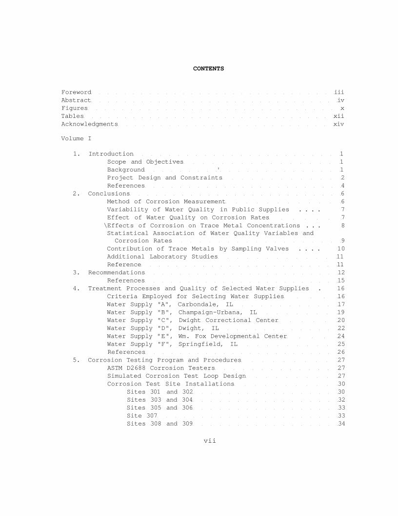
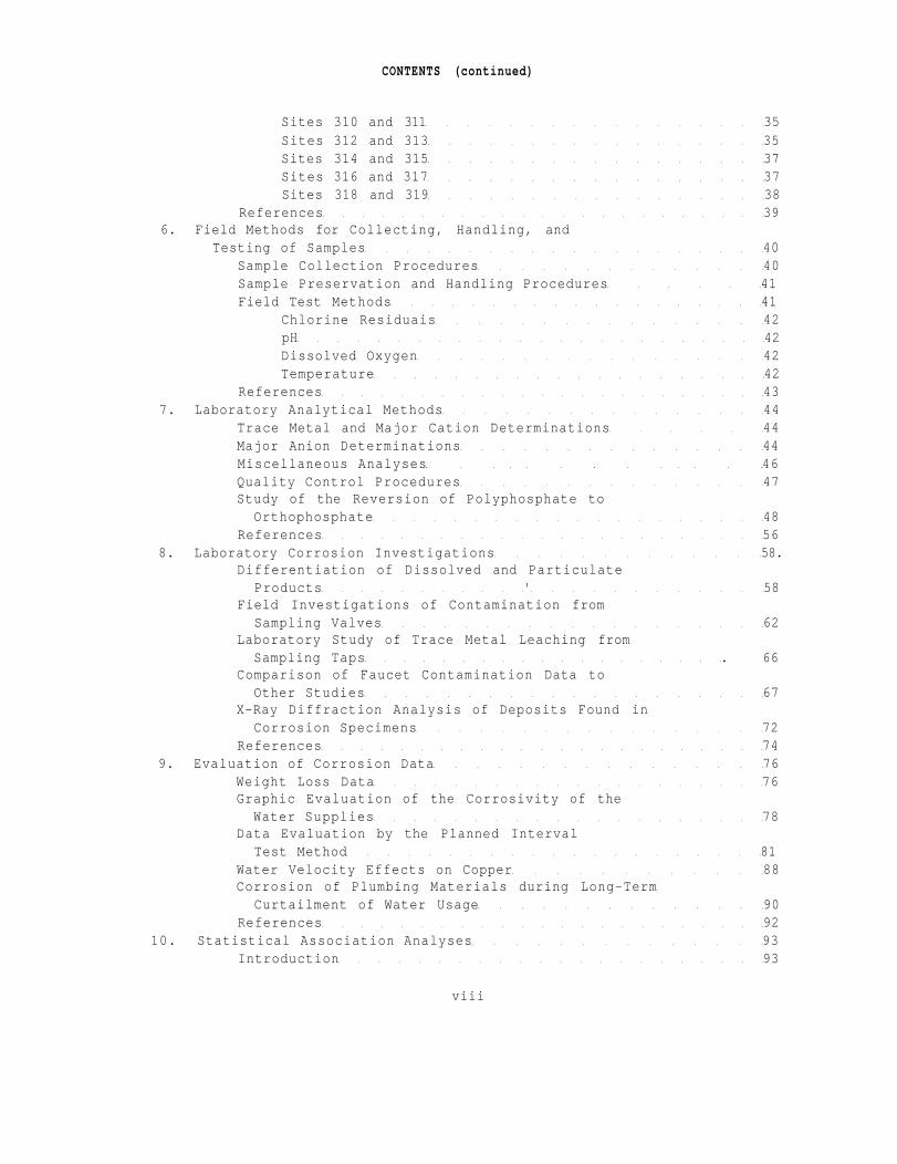