Embed Size (px)
Citation preview

The Pennsylvania State University-
Applied Research Laboratory
PO Box 30, State College, PA 16804
PERFORMANCE MEASUREMENTS ON
A THERMOACOUSTIC REFRIGERATOR
DRIVEN AT HIGH AMPLITUDES
by
Matthew Ernest Poese
and
Steven L. Garrett
Technical Report Number: TR 98- 003 June 1998
Supported by: ARL through the Enrichment and Foundation Program Office of Naval Research NASA through the Pennsylvania Space Grant Consortium
to
Approved for public release; distribution unlimited
[iJTIC QUALITY INSPECTED 1

1. AGENCY UM owtr a#**« ***) 2. REPORT DATE June 1998
4. TTTU ANO SUBTITU
3. REPORT TYPE ANO oAns COVERED Thesis in Acoustics; Master of Science
Performance Measurements on a Thermoacoustic Refrigerator Driven at High Amplitudes
ft. AUTHOR»)
Matthew E. Poese Steven L. Garrett
9. HJNCttNG NUMBERS
7. PERFORMING ORGANIZATION NAMEtS) ANO ADORESS(ES)
Applied Research Laboratory The Pennsylvania State University PO Box 30 State College, PA 16804
*. PERFORMS« ORGANIZATION REPORT NUMMR
TR 98-003
9. SPONSORING /MONITORING AGENCY NAME(S) ANO AOORESS<ES)
Office of Naval Research Ballston Tower 800 North Quincy Street Arlington, VA 22217 Logan Hargrove
Pennsylvania Space Grant Consor 101 S. Frear University Park, PA 16802 Richard Devon, Director
10. SPONSORIG/ MONITOR»*? AGENCY REPORT NUMMR
11. SUPPLEMENTARY NOTES
12«. OiSTRRWTION/AVAfcASRJTY STATEMENT
Approved for public release: distribution unlimited
12b. DiSTRHUTION COOE
13. ARSTRACT (Muamum 200 words) Since the power density in a thermoacoustic device is proportional to the square of the acoustic Mach number, there is strong motivation to design thermoacoustic re- frigerators to operate at larger pressure amplitudes. Measurements are reported of a modified version of the Space Thermoacoustic Refrigerator (STAR), driven at pres- sure amplitudes up to 6%. This pressure ratio corresponds to 30 W of cooling power — five times as large as reported in 1993. The results of these measurements are compared to a DELTAE computer model of the low amplitude (linear) performance that matches experimental conditions on a point-by-point basis. It is found that there is a small but measurable deviation in heat pumping power from the power predicted with a linear acoustic computer model. This deviation in heat pumping power at 6% pressure ratio is about 15%. A large, amplitude independent disagreement in the acoustic power needed to attain a specific pressure ratio is found between measured data and DELTAE results. An overview of the intrumentation, including a measurement of exhaust heat with an absolute accuracy of 65 mW, is also presented.
14. SURJECT TERMS
17. SECURITY CLASSIFICATION OF REPORT Unclassified
IS. SECURITY CLASSIFICATION OF THIS PAGE
Unclassified
19. SECURTTY CLASSIFICATION OF ABSTRACT
Unclassified
15. NUMBER OF PAGES 102
1ft. PRICE COM
20. UMffATKM OF ABSTRACT
NSN 7540-01-280-5500 Standard Form 298 (Rev. 2-89) I t» AHM <M H«.1l

Ill
Abstract Since the power density in a thermoacoustic device is proportional to the square of the
acoustic Mach number, there is strong motivation to design thermoacoustic refrigerators to
operate at larger pressure amplitudes. Measurements are reported of a modified version of
the Space ThermoAcoustic Refrigerator (STAR) [S. L. Garrett, et. al. "Thermoacoustic
Refrigerator for Space Applications," Journal of Thermophysics and Heat Transfer 7(4),
595-599 (1993)], driven at pressure amplitudes up to 6%, which is two times as large as re-
ported in 1993. The results of these measurements are compared to both a DELTAE computer
model of the low amplitude (linear) performance that matches experimental conditions on a
point-by-point basis and one that includes turbulent flow in the duct regions of the device.
It is found that there is a small but measurable deviation in heat pumping power
from the power predicted with a linear acoustic computer model. This deviation in heat
pumping power at 4% pressure ratio is not more than 5% and at 6% pressure ratio is about
15%. The correspondingly poorer coefficient-of-performance is small enough not to deter a
thermoacoustic refrigerator designer from designing for high pressure ratio to take advantage
of the dramatically increased power density. A large, amplitude independent disagreement
in the acoustic power needed to attain a specific pressure ratio is found between measured
data and DELTAE results.
Comparison of low amplitude performance to STAR shows that the modified device has
a coefficient of performance relative to Carnot curve that is shifted downward by approx-
imately 25%. The total amount of heat pumped with the modified device reaches 30 W
which is larger than the amount pumped with STAR by a factor of 5.
An overview of the instrumentation, including a measurement of exhaust heat with an
absolute accuracy of 65 mW, is also presented.

IV
Contents
List of Figures vi
List of Tables vii
Symbol List viii
Chapter 1. Introduction 1
1.1. Background 1
1.1.1. A Short History of Therrnoacoustics 2
1.1.2. Performance Metrics of Thermoacoustic Refrigerators 3
1.2. The Frankenfridge Device 4
1.2.1. Acoustic Subsystem Parameters 6
Chapter 2. Therrnoacoustics on Paper 11
2.1. A Short Heat Engine Primer 11
2.1.1. The Natural Engine 16
2.2. Linear Model in DELTAE 22
2.2.1. Introduction of DELTAE 22
2.2.2. The Frankenfridge Model 23
2.2.3. A More Detailed Look at the DELTAE Solver 28
Chapter 3. Frankenfridge Instrumentation 32
3.1. Sensors and Signal Paths 32
3.1.1. Sensor Calibration History and Cross-Checks 39
3.2. Details of the Exhaust Heat Sink Flange and Flow Loop 43
3.3. The Data Recording System using Lab VIEW 46
Chapter 4. Measurement Analysis and Results 48
4.1. Summary of Experiments 48

4.2. Exhaust Heat Sink Flange 49
4.3. Heat Exchanger Performance Model 56
4.4. Performance of Frankenfridge 61
4.4.1. Performance at low amplitudes (P^/Pm < 3%) 61
4.4.2. Performance at high amplitudes (PAIPW, < 6%) 61
4.4.3. DELTAE Model Perturbations 64
4.4.4. Comparison of Frankenfridge Performance with STAR Perfor-
mance 67
4.4.5. Resonator Losses 69
4.5. Conclusions 71
References 74
Appendix A. Effects of Stack Position on Engine Performance 76
Appendix B. Heat Capacity of the Cold Side Resonator 82
Appendix C. Manufacturer Specifications of Sensors 84

VI
List of Figures Figure page
1.1. Plan view of STAR and SETAC 5
1.2. Cross-sectional view of Frankenfridge 8
2.1. Heat engine schematic 12
2.2. Schematic of the Carnot cycle 13
2.3. Carnot cycle p-v diagram 14
2.4. Schematic of the thermoacoustic cycle 18
2.5. Thermoacoustic cycle p-v diagram 19
2.6. Relationship of stack and parcel temperatures 22
3.1. Work and heat flux in Frankenfridge 33
3.2. Sensor locations on Frankenfridge 34
3.3. Signal paths of instrumentation 40
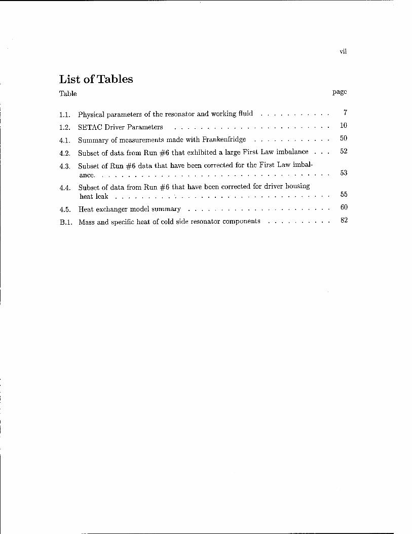
3.4. Schematic of the exhaust heat sink flange and heat flux measurement in- strumentation ■ 45
4.1. Geometry of the hot and cold heat exchanger 60
4.2. Comparison of measured data and DELTAE prediction of Run #4 data .... 62
4.3. Comparison of measured data and DELTAE prediction of Run #6 data .... 63
4.4. Acoustic power requirements in DELTAE models of Run #6 operating con- ditions 65
4.5. Cooling power in DELTAE models of Run #6 operating conditions 66
4.6. Comparison of coefficient of performance relative to Carnot at 2% 68
4.7. Comparison of coefficient of performance relative to Carnot at 3% 68
4.8. Acoustic pressure magnitude and phase of the Frankenfridge DELTAE model . 70
4.9. Resonator acoustic power requirements 71
A.l. Stack performance as a function of stack position in the standing wave ... 80
B.l. Graph of the initial temperature drop in Run #6 83
Vll
List of Tables Table Pa§e
1.1. Physical parameters of the resonator and working fluid 7
1.2. SETAC Driver Parameters 10
4.1. Summary of measurements made with Frankenfridge 50
4.2. Subset of data from Run #6 that exhibited a large First Law imbalance ... 52
4.3. Subset of Run #6 data that have been corrected for the First Law imbal- ance 53
4.4. Subset of data from Run #6 that have been corrected for driver housing heat leak 55
4.5. Heat exchanger model summary 60
B.l. Mass and specific heat of cold side resonator components 82

Vlll
Symbol List
a Sound speed [m/s]
COP Coefficient of Performance
CO PR Coefficient of Performance Relative to Carnot
c Specific heat capacity [j-^<]
/ Frequency [Hz] or Rott function
h Average convective heat transport coefficient [-^^]
K Thermal conductivity [^]
k Wavenumber [1/m]
/ Stack plate half-thickness [m]
M Molecular weight [kg/kmol]
m Mass flow rate [kg/s]
Nu Nusselt number
PA Peak standing wave pressure magnitude [Pa]
px Acoustic pressure [Pa]
pm Static pressure [Pa]
Q Heat energy [J] or resonance quality factor
R Stack radius [m]
Re Reynolds number
7\ Temperature [m]
Tm Mean temperature [K]
m Acoustic particle velocity [m/s]
V Volume [m3]
v Specific volume [m3/kg]
W Work energy [J]
x1 Acoustic particle displacement [m]
xfd Entry length [m]

IX
y0 Stack plate half-separation [m]
ß Coefficient of thermal expansion [1/K]
r Normalized temperature gradient
7 Polytropic coefficient
Ax Stack length [m]
SK Thermal penetration depth [m]
5V Viscous penetration depth [m]
es Stack heat capacity correction factor
r]f Fin efficiency
K Thermal diffusivity [m2/s]
A Wavelength [m]
H Dynamic viscosity [^]
v Kinematic viscosity [m2/s]
pm Mean density [kg/m3]
n Total stack transverse perimeter [m]
a, Pr Prandtl number
ui Angular frequency [rad/s]

Chapter 1.
Introduction
1.1. Background
This thesis focuses on experiments conducted on a small thermoacoustic refrigerator
affectionately called "Frankenfridge."1 Besides being a catchy project name, this moniker
is an apt one because the engine is made of parts from other refrigerators, namely the
Space Thermoacoustic Refrigerator2 (STAR) and the Shipboard Electronics Thermoacoustic
Cooler3 (SETAC), both designed and built at the Naval Postgraduate School. Franken-
fridge is made up from the resonator section of STAR, which includes the stack and heat
exchangers, coupled to a SETAC driver. The STAR driver can produce about 10 W of
acoustic power while the SETAC driver is capable of producing up to 100 W of sound
power. The SETAC driver will allow the STAR resonator to be driven at acoustic pressure
amplitudes much higher than the STAR resonator was originally designed to accommodate.
This thesis experimentally characterizes the performance of Frankenfridge driven at
pressure ratios between one and six percent. The pressure ratio, which is the ratio of the
peak acoustic standing wave pressure in the resonator, PA, divided by the static pressure in
the resonator, pm, never exceeded three percent in the STAR device that flew on the Space
Shuttle Discovery in 1992. SETAC wasn't operated above a four percent pressure ratio
during its sea trials in 1995. Since power density in a thermoacoustic device increases with
the square of increasing pressure ratio, there is strong motivation to design thermoacoustic
refrigerators to operate at higher pressure ratios. It is hypothesized that there are significant
nonlinear effects that alter the performance of the device from the predicted linear response
at pressure ratios greater than four percent.
This experimental treatment attempts to investigate deviations from linear performance
predictions of efficiency and heat pumping power at high pressure amplitudes and to deter-
mine at what pressure ratio these deviations become significant.

1.1.1. A Short History of Thermoacoustics
The interaction of sound and heat was recognized over 200 years ago in the disagree-
ment between Newton and Laplace over whether propagation of sound in air is adiabatic
or isothermal (it is largely an adiabatic process — one of the few times that Newton was
wrong). Glass blowers in the 19th Century noticed freshly blown hot glass bulbs that were
attached to cool stems would occasionally "sing" — this effect was explained by Sondhauss
who qualitatively suggested that there existed a relationship between the pitch of the sound
and the geometry of the bulbs and stems. Sondhauss makes a note in his work of a "glowing
glass harmonica" that preceded his investigation by 40 years. In 1896, Lord Rayleigh ex-
plained the Sondhauss effect and correctly understood the natural phasing of the acoustic
motion, pressure and temperature changes with the conductive heat transfer that could
cause an acoustic oscillation to be sustained. It wasn't until Nicholas Rott and his collabo-
rators worked out a solid quantitative understanding of thermoacoustics (in an attempt to
explain Taconis oscillations) that acousticians were able to create intelligent thermoacoustic
engine designs. A more complete history, with many references, can be found in Swift's7
excellent review of thermoacoustics published in 1988.
The proliferation in the last fifty years of very reliable and inexpensive refrigerators
and air conditioners has led the population of many developed countries to regard cool-
ing machines as a necessity rather than a luxury. Because of these machines' reliance on
CFCs that have been recently found to introduce severe environmental hazards in terms of
ozone depletion and then on HCFCs which have global warming "greenhouse" effects, an
environmentally benign replacement has also become a necessity instead of a luxury. The
thermoacoustic cycle works extremely well with a working fluid of inert gases like helium,
argon and xenon. These three gases are found naturally in the atmosphere and underground
in great quantity (especially helium and argon) and most importantly do not present ozone
depletion or global warming potential. Aside from the environmental benefits, a thermo-
acoustic engine employs little in the way of complicated machinery. The only moving part
in STAR or SETAC is the pusher cone structure in the electro-dynamic driver mechanism.
This piston is different than the pistons in the compressors that power the standard Rankine
cycle refrigerators that are in most kitchens because the thermoacoustic piston is sealed by
a flexure seal and not a sliding seal. The flexure seal is an advantage because it needs no

lubrication and can have a longer lifetime. The thermoacoustic cycle also lends itself well to
a more efficient proportional control, rather than the primitive binary control that conven-
tional refrigerators currently employ. All of these reasons make thermoacoustics potentially
attractive for widespread commercial use.
1.1.2. Performance Metrics of Thermoacoustic Refrigerators
The experiments that are the subject of this thesis are carried out to determine how the
performance of a small thermoacoustic refrigerator (with an ideal gas working fluid) deviates
at high driving amplitudes from the significant and growing body of linear theory that is
valid at low amplitudes. The coefficient of performance, or COP, is one nondimensional
parameter that characterizes a heat engine. One can compare this performance to the
theoretical performance of the same engine operating in a Carnot cycle between the two
thermal reservoirs that correspond to the working temperatures of the actual device. A
ratio that we call "coefficient of performance relative to Carnot" or COPR can be formed
that is the COP divided by the Carnot COP given in Eq. (2.5). Because of turbulent mixing
at the cross-sectional changes in the resonator, for example, it is thought that large drive
amplitudes will degrade the COP for a refrigerator.
Another metric that is of interest to designers of thermoacoustic engines is an expression
for the power density of a thermoacoustic device given by Swift as Eq. 66 in Ref. 7:
H2 f Tmß P (1.1)
V 2{l + es)Pma?
There are several simplifying assumptions that produce this concise expression. Perhaps
the two most gross simplifications are that thermal conduction (heat leak from the hot side
to the cold side) along both the stack material and the gas in the stack is neglected and
secondly, that the viscosity of the gas is assumed to be zero. Other assumptions are that the
stack is short compared to the wavelength of the acoustic standing wave, the temperature
difference across the stack is a small fraction of the mean temperature of the stack and gas,
and that heat and work flows are at steady state. While the steady state assumption is
probably good for Frankenfridge, the no viscosity limit and the short stack approximations
are not very accurate.
By substituting a2 = 7^) into Eq. (1.1),
H2 , (PA (*NJ
1 r J JT Hi 1 V \p
2
fPm -A) (1-2)

it becomes easier to see that the power density increases with the square of increasing pres-
sure ratio, PA/PM- The pressure ratio is a convenient measure of how hard the engine is
being driven — PA is the magnitude of the standing wave pressure at a pressure antinode
and pm is the ambient pressure in the resonator (which in Frankenfridge is about 10 at-
mospheres). This relationship tempts the designers of thermoacoustic engines to increase
this drive ratio (or pressure ratio) of their engines to get more power out of a smaller box.
Because of nonlinear effects such as turbulence, the expression in Eq. (1.2), which is valid
in only a linear domain, will predict extraordinary power densities that cannot be achieved
in a practical device. It is hypothesized that there is some pressure ratio above which the
heat pumping power shows a systematic degradation compared to the above simple expres-
sion. It is the charge of this experimenter to find that critical pressure ratio in the STAR
resonator (Frankenfridge).
1.2. The Frankenfridge Device
As mentioned above, Frankenfridge is a marriage of a small, simple quarter wavelength
resonator to a driver designed to power a much larger capacity thermoacoustic refrigerator.
The STAR device is powered by a driver capable of producing 10 W of acoustic power — the
SETAC driver can produce up to 100 W. In his infinite wisdom, the principal investigator on
both the STAR and the SETAC projects made the bolt circle of the flange that couples the
resonator to the driver equivalent in both devices so as to make the parts interchangeable.
Schematics of STAR (on the left) and SETAC (on the right) are shown in Fig. 1.1
STAR flew on the Space Shuttle Discovery in January 1992 as a part of the Get-
Away Special payload program. After surviving the rigors of launch, STAR operated
autonomously in low-earth orbit. In ground-based tests, STAR spanned a temperature
difference of up to 81 K and pumped up to 5 W of heat. It was generally operated at a
mean pressure of 1 MPa of a helium (97.2%) and xenon (2.8%) gas mixture or a helium
(91.1%) and argon (8.9%) mixture. The device saw acoustic pressure amplitudes up to
2 kPa (which is a pressure ratio PA/pm of 2%). The best coefficient of performance relative
to Carnot {COPE) attained by STAR2 was about 16% at a heat load of 2.8 W.
SETAC sailed in April of 1995 on the USS Deyo (DD-989), a Spruance Class Destroyer,
and cooled the CV-2095 shipboard radar electronics rack. At its peak operating power

eianoisi-
Figure 1.1: Schematic of STAR (left) and SETAC (right). Frankenfridge uses a SETAC driver and the STAR resonator. (Source: Ref. 2 and Ref. 3 respectively)
aboard ship, SETAC provided 419 W of cooling power and spanned a temperature difference
of about 10 K. The refrigerator operated at 2 MPa of a helium (94%) and argon (6%) gas
mixture. SETAC saw acoustic amplitudes of up to 82 kPa (a pressure ratio of 4%.) At the
400 W operating point, a COPR of about 8.2% was realized3. At a lower power and larger
temperature span, the COPR reached 17% based on external reservoir temperatures and
27% based on stack temperatures.

1.2.1. Acoustic Subsystem Parameters
Table 1.1 lists some of the more relevant information about the gas and resonator
of Frankenfridge at the standard operating point. A cross-sectional view of the device is
pictured in Fig. 1.2.
The SETAC driver is instrumented with a microphone positioned very near the pusher
cone and an accelerometer mounted directly on the pusher cone. The signals from these
two sensors allow the measurement of acoustic input power as well as the stroke of the
pusher cone and the acoustic impedance that the resonator presents to the driver. The
resonator is instrumented with thermocouples and semiconductor diode thermometers to
measure the external metal temperatures near the hot (exhaust) and cold (heat load) heat
exchangers. There are no sensors mounted directly inside of the resonator. As pointed
out in Fig. 1.2, the resonator is equipped with a small Kapton tape resistance heater just
below the cold side heat exchanger. This electrical heater provides an easily controlled and
measured amount of heat for the refrigerator to pump. A more detailed explanation of the
instrumentation, including the supporting electronics, signal paths, and computerized data
acquisition system is provided in Chapter 3.
The only new component that is part of Frankenfridge is the copper exhaust heat sink
shown in Fig. 1.2 sandwiched between the SETAC driver and the STAR resonator. This
1/2 in. thick flange has two loops of 1/8 in. copper refrigeration tubing wrapped and soldered
around its perimeter to allow water to be circulated around the flange. The water that is
pumped through this loop and around the flange will absorb some of the exhaust heat and
will therefore experience an increase in temperature as it travels around the flange. The
circulation loop is instrumented with a ten junction thermopile (located directly across the
inlet and discharge ports of the flange piping) and an in-line flow meter located among the
Tygon™ tubing that plumbs the pump, filter and dissipating heat exchanger in the loop.
Based on a measurement of the temperature difference and fluid flow rate, the heat, flux
from the exhaust flange to the water flowing in the loop can be measured. This direct
measurement of exhaust heat flux was not made when the resonator was part of STAR.
The original STAR device was insulated in a vacuum cannister4 which meant that knowing
the heat flux introduced by the Kapton heater and the acoustic power provided by the

Parameter Symbol Value Units
Mean Pressure
Mean Stack Temperature
Gas Mixture (Helium/Argon)
Gas Mixture Atomic Mass
Gas Mixture Density
Gas Mixture Sound Speed
Gas Mixture Specific Heat
Gas Mixture Polytropic Coefficient
Gas Mixture Prandtl Number
Gas Mixture Kinematic Viscosity
Gas Mixture Thermal Conductivity
Stack Thermal Conductivity
Stack Specific Heat
Stack Material Density
Stack Plate Thickness
Stack Plate Separation
Stack Length
Center Position of Stack (ref. from driver)
Stack Radius
Stack (Spiral) Perimeter
Stack Heat Capacity Correction
Cold Exchanger Length
Hot Exchanger Length
Exchanger Fin Thickness
Exchanger Fin Separation
Operating Frequency
Gas Thermal Penetration Depth
Stack Thermal Penetration Depth
Gas Viscous Penetration Depth
Pm 1.07 MPa
T 290
85.5% He
K
M 9.214 kmol
P 4.105 Ja. m3
a 660.4 m s
Cp 2256 J kg-K
7 1.667
a 0.428
ß 2.10 x 10⁻⁵ s-m
K9 0.111 W m-K
Ks 0.161 W m-K
Cs 1101 J
kg-K
Ps 1348 m3
21 0.0762 mm
2y0 0.191 mm
Ax 78.5 mm
xs 206.3 mm
R 19.1 mm
n 4846 mm
es 0.067
Axc 6.35 mm
AxH 2.54 mm
2lEX 0.254 mm
2y$x 0.508 mm
1 328 Hz
6K 0.108 mm
6S 0.010 mm
sv 0.070 mm
Table 1.1: Physical parameters of the resonator and working fluid

SETAC Driver
STAR Resonator
Aluminum Driver Housing
Driver Magnet Structure
Bellows
Pusher Cone
Copper Exhaust Heat Sink
Exhaust Heat Exchanger
Stack
Load Heat Exchanger
Kapton Heater (Heat Load)
Trumpet
High Compliance Termination
Figure 1.2: Cross-sectional view of Frankenfridge. Approximate height is 56 cm and maximum width at the driver housing is 23 cm.

drivert was enough to know the exhaust heat flux (from the First Law of Thermodynamics,
see Eq. (2.1)). Because Frankenfridge has not nearly as "perfect" an insulation scheme,
it is not certain that all of the heat provided by the Kapton heater is pumped by the
fridge or, conversely, that the fridge is not pumping heat from the room. While an attempt
is made to insulate the refrigerator using standard Corning Pink fiberglass construction
grade insulation, for large temperature differences between the cold side duct and room
temperature, heat leak to the cold side is expected. Knowledge of the exhaust heat flux
will allow calculation of the heat leak as well as providing an accurate determination of the
amount of heat that the refrigerator pumps.
The resonator, the new exhaust heat sink, and a 1/8 in. thick Delrin™ insulating ring
are bolted to the driver with eight 1/4 - 20 bolts on a 3.440 in. diameter bolt circle that
is common to the SETAC driver and the STAR resonator. Thermal insulation between the
exhaust heat sink and the aluminum driver housing is critical if a temperature increase is
to be measured in the exhaust heat sink flange. To this end, the 1/4 in. holes have been
enlarged to 5/16 in. to allow for an insulating air gap and the bolt heads have been insulated
with nylon washers from the resonator flange to minimize thermal conduction between the
resonator and the driver housing. The driver housing is not insulated from the room.
The SETAC driver is capable of producing 100 W of acoustic power. It has an invacuo
mechanical resonance frequency of 316 Hz. The pertinent driver parameters are listed in
Table 1.2. The voice coil is attached to a reducing cone that ends in an aluminum piston
face. This cone is attached to the driver housing with a two convolution electroformed nickel
bellows that provides a flexure seal for the resonator and eliminates the need for a sliding
seal. There is a capillary leak between the back volume of the driver and the volume of the
resonator so that the 10 atm of static pressure can equilibrate the driver back volume and
not displace the bellows. The bellows does seal the acoustic pressure in the resonator from
the driver back volume, however.
The sinusoidal electrical signal supplied to the driver originates from an HP 3314A signal
generator and is amplified by a Techron 7520 Power Amplifier. There are no electronics to
control the frequency of this signal to keep the standing wave at the resonance frequency of
the combined driver/resonator system — a frequency that is changing significantly with the
t The STAR driver, although only capable of supplying 10 W of power, was instrumented in much the same way as the SETAC driver.

10
Table 1.2: SETAC Driver Parameters
Parameter Value Units Relative Uncertainty
Moving mass 36.4 g 0.8%
Stiffness 143 kN/m 0.5%
Mechanical resistance 2.10 kg/s 0.6%
Bl 19.1 N/A 0.7%
DC electrical resistance 1.677 n negligible
Effective bellows area 21 cm2 3%
changing temperature of the gas in the fridge (as the fridge gets cold, so does the working
fluid!) In STAR and SETAC a phase-lock loop circuit compared the driver microphone and
accelerometer signals to determine the resonance frequency of the resonator. Frankenfridge
uses a human controller to accomplish this task — the human controller looks at a Lissajous
pattern on a scope that is tracing the accelerometer and microphone signals (to assure a 90°
phase relation of acceleration and pressure, or 0° phase difference of velocity and pressure).
There are many reasons to stay on resonance, not the least of which is that the stack
position in the standing wave is a strong function of heat pumping power. This position
is calculated and designed to be a constant parameter for the system at resonance and if
the frequency is not changed to accommodate the changing sound speed of the gas mixture
this stack position in the standing wave will vary with temperature. Another reason for
resonant operation is that the driver delivers the most power when it operates close to its
mechanical resonance frequency.

Chapter 2.
Thermoacoustics on Paper
2.1. A Short Heat Engine Primer
To begin with some terminology, this thesis will refer to a thermodynamic cycle as the
theoretical picture of the thermodynamic processes that combine to form a cycle, while a
thermodynamic engine is the physical incarnation of this cycle. Often the cycle on which an
engine is based is not exactly the cycle that the engine follows — engineers sometimes have
to make approximations to the theoretical cyclic representation when using real hissing
steam, clanking gears and sliding pistons. In fact, in the case of the cycle proposed by
Rudolf Diesel in 1893, nobody to date has been able to make an engine that follows his
cycle — the Diesel engine that is in widespread use today does not really follow the Diesel
cycle. The other bit of nomenclature to settle upon is the term engine: this thesis is going
to call any thermodynamic machine an engine no matter whether it works in either of two
possible modes. These modes are pictured in Fig. 2.1: a prime mover, in which the engine
turns the potential energy of a temperature difference into usable work, and a heat pump,
where the engine accepts energy in the form of work and uses the work to pump heat from
a cold temperature reservoir to a hot temperature reservoir. From the thermodynamic
cycle point of view, these two modes are just the opposite of one another; the flow of
heat and work are reversed. In this respect, any idealized thermodynamic engine cycle is
functionally reversible, however few practical heat engines can be made to run backwards
— an automobile engine can't be used as a refrigerator nor can an air conditioner power a
Cessna.
To get started, let's consider the Carnot5 cycle, which was proposed by the Frenchman
Sadi Carnot in 1824, and has become known as the most fundamental and simple thermody-
namically (and functionally) reversible engine cycle that operates between two temperature
reservoirs. The cycle is characterized by alternating two adiabatic steps and two isothermal
steps: for the cycle as it operates as a refrigerator the steps are as follows:

12
\ w
Refrigerator Prime Mover
Figure 2.1: Schematic of a heat engine functioning as a refrigerator and a prime mover
Step 1-2: The gas is expanded isothermally at Tc while receiving energy Qc from
the cold reservoir by heat transfer.
Step 2-3: The gas is compressed adiabatically until the gas temperature is TH.
Step 3-4: The gas is compressed isothermally at TH while it gives up energy QH to
the hot reservoir by heat transfer.
Step 4-1: The gas expands adiabatically until the gas reaches a temperature Tc.
This cycle can be visualized physically (see Fig. 2.2) by considering a cylinder filled with
an ideal gas and a piston that can compress or expand this gas, which is known as the
thermodynamic medium or working fluid. Also consider that this well insulated cylinder
can be alternately brought into contact with two large heat reservoirs, one at temperature
Tc and one at temperature TH, that have infinite heat capacity. Let's follow the heat and
work flux from the point of view of the gas in each of the four stages.
Step 1-2: The gas does work dW on the surroundings in an isothermal expansion
and receives heat dQc from the cold reservoir.
Step 2-3: The gas is worked on by the surroundings with the amount of work dW"
and no heat is transferred while the working fluid temperature is raised
from Tc to TH.

13
Step 3-4: The gas is again worked on by the surroundings with the amount of work
dW and heat dQH is transferred isothermally from the gas to the reservoir,
also at TH-
Step 4-1: The gas does work dW" on the surroundings, no heat is transferred, and
its temperature is reduced to To-
Isothermal Expansion Adiabatic Compression Isothermal Compression Adiabatic Expansion
'dQc
Cold Reservoir, Tc
Figure 2.2: Carnot cycle using a piston and cylinder
These four steps can be represented on a diagram that plots the pressure of the gas as
a function of the volume of the gas — this type of chart is referred to as a p-v diagram
and is quite standard in thermodynamic engine analysis. The qualitative p-v diagram of a
Carnot cycle is shown in Fig. 2.3.
The shaded area inside the p-v diagram represents the amount of work done in one
cycle (the integration of pdV through a complete cycle). This work can be seen in Fig. 2.2
to be dW" - dW" + dW - dW which reduces to dW - dW. The negative signs mean that
work is done by the gas, positive work is defined here as work done to the gas. Because
this net work is done to the gas, heat is transferred "uphill" meaning that heat is taken
from the cold reservoir and exhausted to the hot, against the grain of Mother Nature. The
net amount of heat that is transferred is dQc + (-dQH)- Since dQc < dQH (see Eq. (2.2)
below) the net amount of heat transferred is negative, meaning that a net amount of heat
is transferred from the gas to the surroundings. Although there is heat extracted from the
cold reservoir to the gas, more heat is exhausted from the gas to the hot reservoir. The

14
pressure
volume
Figure 2.3: Carnot p-v Diagram
magnitudes of these heat transfers are guaranteed by the First Law of Thermodynamics
which states that the amount of work done to the gas (or anything inside of a control
volume) plus the amount of heat transferred to the gas plus any change in internal energy
of the gas must be equal to zero:
dQ + dW + dU = 0 (First Law for a control volume) (2.1)
In a thermodynamic cycle that operates at steady state, the state of the system at the
end of the cycle must be the same state at which the cycle began. Therefore, the net change
in internal energy of the gas dll must be zero. This fact reduces Eq. (2.1) to the following
expression of the First Law.
QH = (W- W) + Qc (2-2)
The efficiency of a prime mover or the coefficient of performance (COP) of a refrigerator can
both be expressed in words as the ratio of "How much energy (in the form that I desire) I get
out of the engine compared to how much energy I have to put into the engine." From Fig. 2.1
the efficiency of a prime mover can easily be seen to be W/QH and the COP is Qc/W (if

15
the heat pump is a refrigerator) t. The First Law puts no limits on the relative magnitudes
of these quantities and from Eq. (2.1) it would appear that if built well, the efficiency of a
prime mover or refrigerator could be 100%! However, we know from experience that 100%
efficiency is hard to come by. Indeed, there is a fundamental limit of efficiency: the COP of
an ideal cycle depends only on the operating temperatures (in this case the temperatures
of the thermal reservoirs). This limit is guaranteed by the Second Law of Thermodynamics
which requires that the universal amount of entropy (/ dQ/T) can only grow or remain the
same (much like taxes). The Second Law looks like this for a thermodynamic cycle:
QZ<9£ (for a prime mover) (2.3a) TH TC
9£<9^L (for a heat pump) (2.36) Tc TH
In the Carnot cycle, the amount of entropy generated in one isothermal step exactly
balances the entropy decrease in the other step and the adiabatic steps generate no entropy.
The Carnot cycle is said to be thermodynamically reversible because no entropy is generated.
The solution of these expressions for the First and Second Laws gives a measure of the
efficiency or COP of the cycle, and these are:
yrr rp rp Efficiency (prime mover) = —— < —— (2.4)
QH J-H
COP (refrigerator) = ^ < T° (2.5)
In general, real engines never get close to this efficiency, and in fact only theoretical
thermodynamically reversible engines ever attain an efficiency (or COP) equal to that up-
per limit. This upper limit of efficiency is called the Carnot efficiency (or Carnot COP
for a refrigerator). A cycle is considered to be thermodynamically reversible if all parts
of the system are in equilibrium at all time. Some examples of a reversible cycle are the
Carnot and Stirling cycles. In order for this Carnot cycle to be reversible, the heat transfer
processes from the gas to the thermal bath must take place at only a miniscule temperature
difference. Likewise, the adiabatic compressions and expansions must occur over infinitely
t The difference W - W will simply be referred to as W, the net work done on the gas.

16
long time periods. These dreamy reversible processes that are called quasi-equilibrium pro-
cesses really inhibit any power that the cycle might produce if made into a physical engine.
Engineers must sacrifice these quasi-equilibrium processes for much faster methods of energy
conversion and heat transfers that have irreversibilites, like explosions of gasoline vapor in
most automobile engines, free expansion of compressed gas in a household refrigerator and
in a thermoacoustic engine, non-zero temperature differences across the heat exchangers.
The conversion from an on-paper cycle to a real greasy, rumbling and rattling engine lowers
this best-case efficiency, but in exchange lets the engine produce work at a rapid enough rate
to be usable. This is a manifestation of the fundamental trade-off between efficiency and
power in heat engines and illustrates that the operating point of maximum power output is
not the operating point of best efficiency.
Another source of irreversibilites encountered in converting a cycle to an actual engine is
the mechanism that provides the phasing of the thermodynamic steps — a mechanism that
often makes an otherwise functionally reversible cycle into an engine that can only function
in either the prime mover or refrigerator mode. In an automobile engine, the timing belt
and piston lever arms (among other things) contribute to the temporal separation of the
expansions and compressions of the working fluid. In a conventional refrigerator, check
valves and nozzles ensure the flow of refrigerant in the correct direction. Rather than put
up with thermodynamic irreversibilities as a necessary evil, a class of reciprocating heat
engine cycles called natural engines use these irreversibilites to provide the phasing of the
heat and work flows through the cycle6.
2.1.1. The Natural Engine
This brings us around to the thermoacoustic heat engine — a very elegant natural
engine that requires few moving parts because the Good Mother has provided the phasing
mechanism for us. The natural heat engine cycle has one fundamental hardware difference
with reversible heat engine cycles: the presence of two thermodynamic media. In the
thermoacoustic cycle, one medium is the oscillating working fluid (noble gas mixtures,
liquid sodium, and air are three examples) and the other is a stationary medium which in
Prankenfridge is a set of parallel Mylar™ sheets. In a thermoacoustic device, the term
coined for this second medium is the stack — the term comes from the first thermoacoustic
devices which used a stack of parallel plates as the second thermodynamic medium.

17
The phasing in the thermoacoustic engine is ensured through the fact that the irre-
versible thermal conduction between the gas and the stack is not instantaneous but takes
some finite time which is on the order of one quarter of an acoustic period. This lag between
the heat flow and the acoustic gas oscillation is the phase difference that allows the engine
to either absorb or generate acoustic workJ
The thermoacoustic cycle can be thought of in terms of four distinct stages as illustrated
in Fig. 2.4, two adiabatic changes in pressure and two constant pressure heat transfer steps
— the four steps which make up the Brayton cycle. In reality, the thermoacoustic cycle
differs because the sinusoidal oscillations of the gas are always in contact with the stack
which tends to blur the separation of these different steps. However, if these sinusoidal
oscillations are replaced with square wave oscillations, the resulting articulated cycle can
be more easily described in Fig. 2.4 and in words below:
Initially: The stack and gas are at the same temperature, T and the pressure
in the resonator is p0. Once the standing wave is introduced, the
pressure at the initial position of the gas parcel increases to some
value above pQ which is labeled p.
Step 1-2: The acoustic standing wave does work dW" on the parcel of gas to
both compress it adiabatically to pressure p + 2pi and simultane-
ously translate it a distance 2^!. The temperature of the gas parcel
increases adiabatically by 2Tj due to the pressure rise.
Step 2-3: As the gas slows down and stops to change direction, it transfers
heat dQH by irreversible thermal conduction to the stack which is
at a lower temperature than the gas. This thermal conduction is a
constant pressure process which lowers the gas temperature by an
amount dT and increases the volume of the parcel.
Step 3-4: The acoustic standing wave picks up the parcel and returns it a
distance -2xx to its starting place. Because it has moved to a
point of lower pressure it expands adiabatically during this move
t It could be successfully argued that the hot and cold reservoirs in the Carnot cycle constitute a second thermodynamic media. In those terms the difference between the Carnot and the thermo- acoustic cycle is that in the thermoacoustic cycle, the first thermodynamic medium (the working fluid) is in constant contact with the second medium (the stack).

18
Step 4-1:
and returns energy dW" to the standing wave in the form of work.
Since the pressure of the parcel has decreased, the temperature is
also lowered by an amount TTX.
The parcel of gas which is again slowing down or at, rest while
changing direction absorbs heat away from the stack by conduction
because it is colder than the region of stack nearest the gas. Because
of this conduction, the gas takes up a bigger volume at a pressure
p and returns work dW to the standing wave.
Acoustic Pressure Scale
lPl|--
0--
"Pi"
Stack.
Half-wavelength Resonator
/
/ Sinusoidal Acoustic Pressure
=^ -Magnified single stack plate (shown below)
Adiabatic Compression Constant Pressure Adiabatic Expansion and Translation Expansion and Translation
■=n i , r i i ~r Stack Plate
dW'
Gas Parcel
Q= 2x,
y 1dQH
,-v dW
T + 2T„
P +2Pl
T
P
T + 2T -dT
P + 2p,
_—— —» 2x.
T + 2T -dT
P +2p,
3 C
dW
Constant Pressure Compression
T- dT
P
dW
dQr
Figure 2.4: Articulated thermoacoustic refrigeration cycle in a Lagran- gian reference frame
The p-v diagram for this articulated thermoacoustic cycle, or Brayton cycle, is shown
in Fig. 2.5, along with the p-v diagram for the ideal thermoacoustic cycle where the parcel
follows the more realistic sinusoidal motion (as opposed to square wave motion in the
articulated cycle description.)

19
Articulated Thermoacoustic Cycle pressure (Also the Brayton Cycle)
3 2 P + P, ~
\\
P - 4* ' 1
pressure
p + p,
Ideal Thermoacoustic Cycle
volume volume
Figure 2.5: The p-v diagrams for the exaggerated and sinusoidal thermo- acoustic cycle
The proper phasing in this natural engine, as mentioned above, is ensured because the
thermal conduction does not take place instantly, but introduces some time lag between
the conduction and the motion/pressure changes. The amount of heat that is conducted
from the gas to the stack or vice versa depends upon the distance that separates the gas
parcel from the stack in a direction perpendicular to the stack plates. The parcels of gas
that oscillate very close to a stack plate transfer heat in a locally isothermal and reversible
way while the parcels that are very far away from the plates don't have any thermal contact
with the stack and are simply adiabatically expanded and compressed by the standing wave.
But, there obviously exists a "sweet spot" where a parcel of gas is far enough away so that
thermal contact is poor enough that the heat transfer rate introduces the needed phase
relationship, but near enough to not be completely insulated from the stack. This sweet
spot is referred to as a thermal penetration depth and is defined as:
SK = (2.6)
where u is the angular frequency of the gas oscillation and K is the thermal diffusivity
(K = K/pmcp and K is the thermal conductivity) of the gas. This length can be thought of
as the distance that heat can diffuse through the fluid in a time ^-.
Since the acoustic excursion, 2xi, is on the order of a few millimeters in the Pranken-
fridge device and the stack is several centimeters long (7.85 cm to be exact), it is apparent

20
that one parcel of gas doesn't really get the job done of spanning a temperature difference
larger than 2TX or pumping any more heat than a measly dQc\ Because there are many such
parcels lined up along the length of the stack, the parcels work like bucket brigade shuttling
only a small amount of heat each. The end result can be temperature differences across the
stack that have reached 36°C and heat pumping powers of 30 W in this experiment.
This bucket brigade effect illustrates that an important material property of the stack
is low thermal conductivity in the direction of acoustic propagation. If the stack were made
of copper it would never be able to sustain a temperature difference across itself — the
bucket brigade would be trying to fill a very leaky tub! At the same time, however, the
stack must be able to conduct heat in a direction perpendicular to the acoustic flow in
order to absorb and release heat to and from the gas parcels. This combination of adequate
insulation in a longitudinal direction but sufficient conduction in the lateral direction is
more or less satisfied by Mylar™ (in the case of this thesis), stainless steel, the ceramic
used in catalytic converters and even coffee stirring sticks!
To round out this mostly qualitative discussion of the thermoacoustic cycle, the func-
tionally reversible nature of the cycle should be mentioned. A thermoacoustic device that is
attached to a speaker or other type of linear motor can be a refrigerator if this driver excites
a standing wave in the resonator. On the other hand, if a temperature difference is imposed
across the stack by outside means, the device will produce sound (acoustic work) and will
function as a prime mover. Two temperatures are important to the parcel of gas — it's
own temperature at the end of an adiabatic compression or expansion and the temperature
of the stack at that location. If the parcel is compressed (and heated to a temperature
T + 2Ti by the standing wave), and finds that the stack is hotter than it is, then the stack
will transfer heat energy to the parcel. Since the pressure is higher where the parcel is
expanded, net work is added to the acoustic standing wave and this is the prime mover
mode. On the other hand, if the parcel of gas sees a portion of stack that is colder than it
is (the situation illustrated in Fig. 2.4), then the work and heat flows are the opposite of
the prime mover and we call this the refrigerator (or heat pump) mode. Obviously then,
there must be some stack temperature gradient that is the line of demarcation between a
prime mover and a refrigerator. This temperature gradient is called the critical temperature

21
gradient and is defined as:
VTcrü = Z^El. (2.7)
For sinusoidal pressure and velocity oscillations which occur in an acoustic standing wave
(and which is assumed throughout this thesis) this ratio pi/uj can be reduced to pma cot{kx)
(where x is the position of the stack in the standing wave relative to the pressure antinode
of the fundamental mode and A; = 2n/X is the wavenumber). Thermodynamic calculations
show that7 7 - 1 = Tmß2a2/cp, so that another expression of the critical temperature
gradient is:
VTCTit = '^Tmk cot (kx). (2.8)
Especially for gases, (7 - 1)/Tmß is very close to unity (for ideal gases, Tmß is exactly
unity) and cot(kx) for reasonable stack positions is between 1 and 10 which makes the
critical temperature gradient on the order of Tmk = 2irTm/X. This useful approxima-
tion tells us that the critical temperature gradient for the device in this thesis is around
(290 K)(3.04 m_1) = 882 K/m. For a stack length of 7.8 cm, the stack temperature differ-
ence below which this device is refrigerator and above which it is a prime mover therefore
about 70 K.
What happens when the engine operates at this stack temperature difference exactly?
As a parcel of gas is compressed, it's increase in temperature exactly matches the tem-
perature of the stack along it's path and no heat is transferred to the parcel. Operation
very close to this critical temperature difference is the most efficient point for the engine;
however, this operating point pumps almost no heat in the refrigerator mode or conversely,
produces very little work in the prime mover mode. The relationship between stack and
parcel temperatures is illustrated below in Fig. 2.6.
A real refrigerator is usually built with a stack and a driver as mentioned above. The
stack is housed in a tightly sealed resonator and two heat exchangers are coupled to the
ends of the stack. (It is these heat exchangers that are largely responsible for the efficiency
decrease in going from an on-paper cycle to a humming engine that can make your beer
cold). An important thing to note at this point, only because it has not yet been mentioned
explicitly, is that a thermoacoustic refrigerator is operated at the resonance frequency of the
combined driver/resonator system. This fact is important because the resonance enhances
the acoustic wave generation for a given excursion of the pusher cone — which means that

22
Refrigerator
Critical Gradient
Figure 2.6: Relationship of stack and parcel temperatures for heat engine mode determination
the movement of the pusher cone in the driver can be quite small and still generate large
acoustic pressure amplitudes. This fact also allows a flexure rather than a sliding seal to be
used. Resonant enhancement is a fundamental distinction of the thermoacoustic cycle that
is not shared with many other reciprocating heat engine cycles.
2.2. Linear Model in DELTAE
2.2.1. Introduction of DELTAE
The software package DELTAE (which stands for Design Environment for Low-Amplitude
Thermoacoustic Engines8) is a text based program written by Drs. Bill Ward and Gregory
Swift at Los Alamos National Laboratory that estimates the performance of a thermoacous-
tic device. A model in DELTAE comprises a series arrangement of transducers (drivers),
ducts, heat exchangers, thermoacoustic stacks, and compliances (or any impedance tran-
sition.) For each of these segments, the computer solves a one dimensional wave equation
with temperature evolution by matching the pressure, volume velocity and temperature
at the interface of each segment as boundary conditions. In thermoacoustic elements (the

23
stack), the program also solves the enthalpy flow equation to find the temperature profile
along the stack.
Once the user has completed the geometric model of the device using either the very
basic text user interface (TUI, I suppose?) of DELTAE or any text editor, the user must
initialize a set of vectors called the Guess and Target Vectors. It has been said that DELTAE
is to the thermoacoustician what a souped up Ferrari is to a sports car enthusiast. If this is
true, these vectors are the equivalent of the clutch and the accelerator pedals. By stipulating
what quantity or quantities are fixed Targets, and which quantities DELTAE is allowed to
vary to reach those Targets (the Guesses), the user drives this model to learn what the
coefficient of performance (COP), temperature span or heat load can be for the device. If
the user is designing a device instead of modeling an existing device, he can let the stack
position be the Guess vector and in this way determine the optimum stack position for a
given heat load or coefficient of performance.
2.2.2. The Frankenfridge Model
It will be much easier to comprehend the structure of DELTAE after the model has been
explained and the DELTAE model file is examined. The model appears below as it does in
the DELTAE TUI. This file is called the *.out file, and is generated each time that the user
runs the model.
TITLE FF-M1 Straight Frank ->frankv2.out CreatedSlO: 7:17 18-Mar-98 with DeltaE Vers. 4.0b7 for the IBM/PC-Compatible 0
BEGIN 1.0770E+06 a Mean P Pa 319.42 A Freq. G( Ob) P 319.42 b Freq. Hz G 6.4114E-05 B |U|®0 G( Of) P 297.44 c T-beg K -0.2366 C HeatIn G( 6e) P
4500.0 d IplSO Pa 0.0000 e Ph(p)0 deg
6.4114E-05 f lUlfiO nT3/s G 0.0000 g Ph(U)0 deg
0.855hear Gas type ideal Solid type
j
ENDCAP Sadie 2.1000E-03 a Area m"2 4500.0 A |p| Pa
0.0000 B Ph(p) deg 6.3722E-05 C |U| m"3/s

24
sameas 0 Gas type
ideal Solid type
ISODUCT Bellows
2.0480E-03 a Area m"2 0.3654 b Perim m
1.8900E-02 c Length m
sameas 0 Gas type
ideal Solid type
ISODUCT Insulating Ring
2.9090E-03 a Area m"2
1.1480 b Perim m
3.0200E-03 c Length m
sameas 0 Gas type
ideal Solid type
ISODUCT Interface
1.1950E-03 a Area m~2
0.1988 b Perim m
1.2700E-02 c Length m
sameas 0 Gas type
copper Solid type
ISODUCT HX Flange
1.1400E-03 a Area m~2
0.1240 b Perim m
2.6240E-02 c Length m
sameas 0 Gas type
copper Solid type
HXFRST Exhaust HX
1.1400E-03 a Area m~: 0.5000 b GasA/A
6.3500E-03 c Length m
2.5400E-04 d yO m
-0.2366 e Heatln W
0.0000 D Ph(U) deg
0.1434 E Hdot W
0.1434 F Work W
-8.8274E-04 G Heatln W
4492.6 A |p| Pa
-5.9538E-02 B Ph(p) deg
2.0561E-04 C |U| m"3/s
-72.353 D Ph(U) deg
0.1405 E Hdot W
0.1405 F Work W
-2.9039E-03 G Heatln W
4490.8 A |p| Pa
-6.5926E-02 B Ph(p) deg
2.4846E-04 C |U| m"3/s
-75.637 D Ph(U) deg
0.1390 E Hdot W
0.1390 F Work W
-1.4552E-03 G Heatln W
4466.7 A |p| Pa
-0.1322 B Ph(p) deg
3.2299E-04 C |U| m~3/s
-79.108 D Ph(U) deg
0.1379 E Hdot W
0.1379 F Work W
-1.0722E-03 G Heatln W
4393.8 A Ipl Pa
-0.2774 B Ph(p) deg
4.6986E-04 C |U| m~3/s
-82.675 D Ph(U) deg
0.1366 E Hdot W
0.1366 F Work W
-1.3848E-03 G Heatln W
4344.3 A Ipl Pa
-0.2524 B Ph(p) deg 4.8958E-04 C |U| nT3/s
-83.295 D Ph(U) deg
-0.1000 E Hdot W

25
295.10 f Est-T
sameas 0 Gas type
ideal Solid type
(t)
i.
STKSLAB Stack
1.1100E-03 a Area m" 0.7730 b GasA/A
7.8500E-02 c Length m 1.9100E-04 d yO m
7.6200E-05 e Lplate m
sameas 0 Gas type
mylar Solid type
HXLAST Cold HX
1.1400E-03 a Area m"2 0.5000 b GasA/A
2.5400E-03 c Length m 2.5400E-04 d yO m
0.1000 e Heatln W =8
280.00 f Est-T K (t
sameas 0 Gas type
copper Solid type
INSC0NE Cold Reducer
sameas 8a a Areal m~2
0.1197 b PerimI m
9.2200E-03 c Length m
3.8350E-04 d AreaF m~2
6.9420E-02 e PerimF m
sameas 0 Gas type
copper Solid type
INSDUCT Cold Duct
sameas 9d a Area m"2
sameas 9e b Perim m
0.1400 c Length m
sameas 0 Gas type
copper Solid type j
INSC0NE Horn
sameas 10a a Areal m"2
sameas 10b b PerimI m
6.9220E-02 c Length m
10
11
0.1288 F Work W
-0.2366 G Heat W
297.32 H MetalT K
3723.2 A |p| Pa
1.2014 B Ph(p) deg
8.3121E-04 C IUI m"3/s
-88.138 D Ph(U) deg
-0.1000 E Hdot W
1.7844E-02 F Work W
297.44 G T-beg K
257.31 H T-end K
-0.1110 I StkWrk W
3684.3 A Ipl Pa
1.2823 B Ph(p) deg
8.3796E-04 C |U| m"3/s
-88.196 D Ph(U) deg
0.0000 E Hdot W
1.4055E-02 F Work W
0.1000 G Heat W
257.34 H MetalT K
3572.6 A Ipl Pa
1.2748 B Ph(p) deg
8.6546E-04 C |U| m~3/s
-88.220 D Ph(U) deg
0.0000 E Hdot W
1.3622E-02 F Work W
0.0000 G Heatln W
352.16 A Ipl Pa
0.3915 B Ph(p) deg
9.8603E-04 C IUI m"3/s
-88.335 D Ph(U) deg
0.0000 E Hdot W
3.8601E-03 F Work W
0.0000 G Heatln W
841.36 A Ipl Pa
-178.22 B Ph(p) deg
9.6987E-04 C IUI m~3/s

26
7.4320E-04 d AreaF
9.6630E-02 e PerimF sameas 0 Gas type copper Solid type
m~2 m
-88.340 D Ph(U) deg
0.0000 E Hdot W 8.8184E-04 F Work W
0.0000 G Heatln W
12 COMPLIANCE Bulb 6.8300E-02 a Area 1.0310E-03 b Volum
sameas 0 Gas type
stainless Solid type
m"2 m~3
HARDEND End Impedance
0.0000 a R(l/Z) 0.0000 b Kl/Z)
13
841.36 A Ipl Pa
-178.22 B Ph(p) deg
1.7848E-09 C |U| m"3/s
-76.437 D Ph(U) deg
-1.5328E-07 E Hdot W
-1.5328E-07 F Work W
-1.5328E-07 G Heatln w
=13G?
= 13H?
sameas 0
ideal
Gas type
Solid type
841.36 A Ipl Pa
-178.22 B Ph(p) deg
1.7848E-09 C |U| m~3/s
-76.437 D Ph(U) deg
-1.5328E-07 E Hdot W
-1.5328E-07 F Work W
-1.8297E-08 G R(l/Z)
8.7741E-08 H I(l/Z)
257.31 IT K
The numbered segments that are separated by dashed lines are the series representation
of the elements of the Frankenfridge device. The characters in the upper left hand corner
of the segment are the DELTAE name for the type of segment. Some terms are complete and
their meaning is obvious. The ones that are not follow9:
IS0DUCT
INSDUCT
HXFRST
a duct that is constrained to be isothermal by an energy source or
sink not accounted for by DELTAE.
a duct that is insulated. The heat generated by the thermoviscous
losses in this type of segment is transported onto the nearest heat
exchanger so that DELTAE calculations of coefficient of performance
reflect this deleterious effect.
the first heat exchanger in a system. For a quarter wavelength
device with the stack nearest the pressure antinode, this heat ex-
changer is the hot side heat exchanger. In a heat pump, this
exchanger dumps the exhaust heat plus work (enthalpy) from the
device.

27
HXLAST
STKSLAB
INS/ISOCONE
COMPLIANCE
HARDEND
this is the heat exchanger on the other side of the stack. In the
Prankenfridge configuration this is the cold side heat exchanger,
or the heat exchanger that takes on the heat that the device is
obligated to move. Since it is followed by INSDUCT segments, it
also absorbs the thermoviscous power generated in these segments,
the thermoacoustic stack. There are many varieties of stacks,
many of which DELTAE is capable of modeling. The STKSLAB seg-
ment is for modeling a parallel plate type stack,
just like the duct, but has an initial cross sectional area that is
larger or smaller than its final cross sectional area,
a series impedance that is an acoustic volume. Unlike the ducts
and cones which have both thermal and viscous losses, the com-
pliance only has thermal losses.
this ends a device with a rigid termination that requires that the
volume velocity of the working fluid be identically zero.
The *.out file is divided into two columns: the column on the left is the input column
while the column on the right is the output column which displays the results after the
program is executed. Notice that these quantities in the output column have a capital letter
to designate them. For example, the phase of the acoustic pressure that DELTAE calculates
in segment 8 would be denoted as quantity '8B.' In the input column, the quantities that
describe the geometry and initial values pertinent to each segment are designated with a
lower case letter. The ratio of the cross sectional area available for fluid flow to the total
cross sectional area in the cold heat exchanger is denoted as quantity '8b.' (Remember that
the fins of a heat exchanger occlude some fraction of the cross sectional area.)
It is from the input column of the model file that the Guess and Target vectors come.
As mentioned above, a Guess is a parameter that the user allows DELTAE to vary in order
to get the Target parameter to match the user specified value. A convenient way to think
about the Guesses and Targets is to consider a Target to be something that we think of
as an experimentally controlled variable or a given in the problem. A Guess is something
that we might consider to be an experimental result. The Guesses are used as input to the
DELTAE solver and a Target is a variable that DELTAE computes on every iteration.

28
In the Frankenfridge model as it stands here, there are two entries each in the Guess
and Target vectors. As one might imagine, these vectors must be balanced: there must be
as many Targets as there are Guesses. The Guesses are denoted in the input column with
a capital G next to the parameter of a segment. The values that DELTAE converges upon
for the Guess parameters after a run appear in the output column in segment 0. Possible
Targets are delineated in the input column with a lower case 't' in parentheses, (t), next
to a parameter in a segment. A parameter that has been chosen to be part of the Target
vector is noted in the input column with an equal sign, followed by the parameter in the
output side that functions as a comparator and ends with a question mark. For example,
in the Frankenfridge model, the real part of the admittance at the HARDEND is a target that
should have the value of 0 (we define this condition to ensure that a standing wave exists in
the resonator). This Target is marked with '=13G?' to show that it is a Target and should
be compared to parameter 13G in the output column.
2.2.3. A More Detailed Look at the DELTAE Solver
The DELTAE software models acoustic wave propagation, with temperature evolution,
by integrating the coupled differential equations (shown in the paragraphs below) from the
model's BEGIN segment to the HARD or SOFT END segment with respect to five variables9: real
mean temperature Tm(x), complex acoustic pressure pi{x), and complex acoustic volume
velocity, U^x). For each segment, the algorithm uses the differential equation that governs
that type of segment, using the segment specific (local) user defined variables like geometry
and required enthalpy flow and model (global) variables like mean pressure and frequency.
The boundary conditions used for the solution are the continuity of temperature, pressure
and volume velocity at segment junctions.
If these boundary conditions are known at the beginning of each segment, then this
process is very simple. However, the power of DELTAE is that the user can specify a boundary
condition (or Target) anywhere in the model, even at the end of the last segment of the
model. In the Frankenfridge model, the admittance at the HARDend segment is pinned
to be zero (This is the equivalent of specifying the volume velocity equal to zero at the
wall.) So, lacking enough definite boundary values at the beginning of the BEGIN segment,
DELTAE uses a shooting method whereby the algorithm "guesses" the value of the unknown
quantities and then comparing the finished calculation results with the Target vectors. In

29
this way, the algorithm converges to a solution specified by the user. In fact, DELTAE forms
a non-linear system of equations from the Target vector and massages the Guess vector so
that the difference between the Targets and the results of the calculation are within a user
specified tolerance. The routine that performs this part of the simulation is called DNSQ
and is part of the SLATEC Common Mathematical Library at http://www.netlib.org. This
algorithm is a modification of the Powell hybrid method.9
Instead of integrating one equation — the wave equation with temperature evolution
— DELTAE uses three uncoupled equations: a modified form of Euler's Equation, a modified
form of the continuity of mass equation and an expression of heat transfer that describes
the mean temperature distribution in the gas. In order to present the way that DELTAE
simulates a thermoacoustic device, let's study the wave equation with thermoviscous losses
(the irreversibility that makes the thermoacoustic cycle a useful heat engine) as it applies
in a standing wave resonator with a plate inserted at some point in the standing wave10.
The plate is long in the direction of acoustic propagation and has width but has neg-
ligible thickness. We'll call the direction of propagation the x direction. The dimension
normal to the plate is the y direction and the width of the plate is in the z direction.
The conservation of momentum expression that includes viscous losses is:
<«i> = — (1 - /,) 7T (2-9) up™, ax
The term /„, which is the spatial average of hv, is called by the thermoacoustic community
a Rott function in viscosity7 and it describes how viscosity reduces the magnitude of the
oscillatory velocity near the plate and shifts its phase. For flow along a plate not near an
edge of the plate, (near the middle of a parallel plate stack geometry, for example) this effect
is most prevalent. In the modified Euler's Equation (Eq. (2.9)) above, the term (l-/„) alters
the oscillatory velocity so that gas that is much closer than a viscous penetration depth (6„)
to the nearest solid surface (right next to the surface) is almost at rest. Likewise, a parcel of
gas that is oscillating much farther than Sv from the surface "feels" no viscous shear at all
and has no spatial dependence in the y or z directions. A parcel of gas that oscillates near
a viscous penetration depth away from the wall, however, does so with reduced velocity
and a non-trivial phase shift that opposes phasing of the thermoacoustic transport. It is
much easier, both analytically and computationally, to consider the spatial average in y
rather than to retain the functional dependence since this reduces the integration to only

30
a one dimensional problem. The spatial average of the Rott function for velocity follows in
Eq. (2.10).
tanh
/,=
(1 +1) y0/5v
(2.10) (l + i)y0/6v
Here, y0 is half of the stack plate spacing. Note that Eq. (2.10) only includes a geometrical
parameter and a penetration depth, <5„. The viscous penetration depth, like the thermal
penetration depth defined in Eq. (2.6), defines the length of the effective boundary layer
and is inversely proportional to the square root of frequency.
The conservation of mass equation that is relevant to thermoacoustic heat transport
includes both viscous and thermal dissipation:
dx
IU!
pma' L 1 + (7-1)/K PI +
(/«-/„) 1 dTn <«i) (2.11)
(1 - /„) (1 - a) Tm dx
Here, fK is equivalent to /„ except that it involves the thermal penetration depth rather
than the viscous. That is, thermal contact with the solid reduces the magnitude of the tem-
perature oscillations in the x direction and introduces a significant phase shift. Explicitly,
a parcel of gas that is much less than a penetration depth away from the surface is nearly
isothermal and those far away from the boundary layer expand and contract adiabatically
in phase with the pressure oscillations. Those parcels at about a penetration depth from
the surface are at neither extreme and experience magnitude reduction and a phase shift
(that aids the thermoacoustic transport) with respect to the pressure oscillations. Since
both temperature and velocity fluctuations affect the density gradient in the direction of
acoustic propagation, both viscous and thermal terms make their appearance in the con-
tinuity equation. The first term in the right hand side of Eq. (2.11) describes the density
fluctuations due to pressure oscillations of the gas (and involves only thermal loss) while
the second term includes the density oscillations due to velocity and includes both thermal
and viscous loss.
To complete the system of equations that combine to form the wave equation for thermo-
acoustics (Rott's wave equation), the temperature profile that appears in Eq. (2.11) must
be described:
dTm
dx Anas L Pl(Ül) 1-
(/« - /,) (l-/„)(l + a)
U-'Xf-fA^+^-K-^"'} (2-12)

31
While this is not as intuitively obvious as the two familiar conservation equations, this equa-
tion can be loosely explained physically as follows. The last two terms in the denominator
account for the thermal conduction losses in the direction opposite useful heat transfer
along the stack: one term for conduction in the gas and one for conduction in the solid.
The second term in the numerator represents the acoustic intensity in the standing wave
and also accounts for the magnitude and phase complexities within the boundary layer.
The first term in the denominator is tricky but basically it represents the internal energy
and kinetic energy that is convected along the temperature gradient. This equation is very
muddled and it is difficult to get an intuitive feel for it by considering it term by term. A
more intuitive feel for thermoacoustic theory can be had by considering the "Short Stack"
approximation found in Swift's 1988 paper (Ref. 7) that presents a better explanation of
the subtle points involved in these equations.
The point of all of this is to get an understanding of what DELTAE uses to model the
thermoacoustic cycle. It has been stated that the program numerically integrates the 1-D
wave equation. In fact, it integrates these three coupled equations, in only one dimension,
using a Runge-Kutta technique. This is such a simple problem that it takes no time at
all for the computer to perform and ultimately contributes to the usefulness of DELTAE.
The user can create a model and see the results of a simulation in less than a second on a
Pentium™ processor. Once the user understands how the program works, he or she can
use it much more effectively; that is, since it uses a shooting method to fill in the unknown
boundary conditions it can get "off the track" quite easily if the user lets the model start
at non-realistic or non-intelligent places. It is very frustrating for the new user who may
not have much experience with thermoacoustic refrigerators to know what these realistic
conditions are. Also, big changes in the parameters can cause DELTAE to have a hard
time converging. A big change in gas mixture or driving frequency can drive the model
to either an instability or a mode that doesn't make any physical sense. In these cases
the new user must be careful — the program conveys little warning if it has converged to
a non-meaningful solution. By checking the heat fluxes in the heat exchangers and work
flux along stack for violations of energy conservation as well as making a reality check of
the heat exchanger and gas temperatures, the user can guard against accepting a garbage
solution.

Chapter 3. Prankenfridge Instrumentation
This chapter will detail the instrumentation used to collect data about the performance
of Frankenfridge. The data that is collected using this instrumentation has proven to be
quite "clean," repeatable and consistent with expected results based on STAR performance.
The first section outlines the signal paths for each sensor. Because the measurement of ex-
haust heat is new for the STAR resonator (and is exciting at such low power levels), a
section is included here that outlines the design, instrumentation and calibration of the
exhaust heat sink flange. The last section briefly overviews the Lab VIEW™ Data Acquisi-
tion system. One purpose of this chapter is to provide a resource for future experimenters
working with the Frankenfridge device, or some modification thereof, and for that reason
may be otherwise inexcusably dense. The manufacturer's calibration sheets for the sensors
described below can be found in Appendix C.
To better understand the instrumentation, that for the most part measures the flow of
heat and work in Frankenfridge, it is important for the reader to have an overall idea of
this energy flux. The diagram shown in Fig. 3.1 illustrates the paths of energy flow.
3.1. Sensors and Signal Paths
The numbered paragraphs below describe the instrumentation at the corresponding
numbered point on Fig. 3.2.
1. SETAC Driver: The SETAC driver contains two sensors, a microphone and
an accelerometer, that are central to the measurement of Frankenfridge acoustic
input power, WACS in Fig. 3.1.
1.1. The microphone is an Endevco Model 8514-10 (SN: Not available).
The sensor is a piezoresistive "strain gauge" type that requires an
ultra-stable bias supply to power the four-arm strain gauge Wheat-
stone bridge that is doped on a silicon diaphragm. This bias sup-
ply, as well as the pre-amplification of its signal is accomplished
with a very nice circuit constructed in the lab. See Appendix C for

33
To dissipator
QH+QVC
Flow Loop
From dissipator
iRe{Zin}
■V2,
: -i^ ;§§§§£ i<x§£p|^1 i" R VC
r ACS
H-ext n
Sxxxxxxxxj;
Figure 3.1: Cross-sectional view of Frankenfridge showing work and heat flow.

34
2.1 Flow Meter
2.2, 2.3 Thermopile Assembly
2.4 Endevco8510B-200 Pressure Sensor
3.5 Kapton Heater
1.1 Endevco 8514-10 Pressure Sensor
1.2 Entran EGA-125-1000D Accelerometer
1.3 Type-E Thermocouple
3.1 Type-E Thermocouple
3.2 Silicon Diode Thermometer
3.3 Type-E Thermocouple
3.4 Silicon Diode Thermometer
Figure 3.2: Cross-sectional view of Frankenfridge showing sensor loca- tions.

35
a complete description and of this preamp, the PR100. The Ende-
vco 8514 is a subminiature design that has a diameter of 1.65 mm
and is mounted in the aluminum driver housing. It is a differential
pressure gauge and its reference port is vented to a small volume
which is connected to the back volume of the driver through a
small capillary leak. This venting arrangement, which acts as an
acoustic low pass filter, lets the sensor sense the acoustic pressure
oscillations on its diaphragm but not the large static pressure in
the resonator since the back volume of the microphone is allowed
to equilibrate to the back volume of the driver. (The resonator and
the back volume of the driver are also in static pressure equilib-
rium via a separate capillary.) For this reason, the pressure sensor
can have a small range of only ±10 psia and therefore a higher
sensitivity than a sensor that would have to carry the static pres-
sure as well as the acoustic pressure. The measured sensitivity of
this microphone is 3.45 /uV/Pa at 250 Hz. See Section 3.1.1 for the
calibration history of this sensor. The nominal factory calibration
is reported as 30 ± 10 mV/psi = 4.35 ± 1.45/iV/Pa.
1.2. The accelerometer is an Entran Model EGA-125-1000D (SN: Not
available). The Entran is a also a piezoresistive strain gauge device
based on a semiconductor Wheatstone bridge. It has a very minia-
ture but robust package that is 6.86 mm x 3.56 mm x 3.56 mm.
The accelerometer also uses the PR100 ultra-stable bias supply
and preamp mentioned previously. The sensor is mounted on
the pusher cone assembly (the side that faces away from the res-
onator). The sensor has a range of ±1000 g = ±9800 m/s2 and
a measured (see Section 3.1.1) sensitivity of 23.2 ^j at 15 V
bias. The factory calibration at 15 V bias is reported to be:
0.222 mV/g = 22.6 ^. Since the PR100 supplies a 10 V bias,
not 15 V, the measured scaled sensitivity is 15.5 ^j (at 10 V
bias).

36
1.3. The driver is also equipped with a self adhesive Omega No. SA1-E
Type-E thermocouple mounted on the face on which the resonator
attaches. This thermocouple serves to monitor possible heat leak
to and from the driver to the exhaust heat sink flange as well as to
make sure that the driver does not overheat. This thermocouple
voltage is read with the Keithley 740.
2. Exhaust Heat Sink Flange: The flow loop that encircles the copper exhaust
heat sink is instrumented with five sensors: a flow meter, a thermopile, two
thermocouples and a pressure sensor. The main function of this flange is to
measure the exhaust heat flux, QH in Fig. 3.1. Since the acoustic power is
measured, knowledge of the exhaust heat and the First Law of Thermodynamics
is adequate to determine the heat pumping power from resonator's cold end.
2.1. The flow meter is a Hedland IR-OPFlow Model 502-101 (SN:
none) which is an axial paddle wheel (Pelton wheel) turbine type
flow meter. The sensor has an infrared transmitter and receiver
molded into the body of the meter that provides a square wave
output signal whose frequency is directly proportional to flow rate
(1 pulse per rotation). The amplitude of the square wave is 1.2 V
below the DC bias voltage supplied to the sensor which can be
between 5 V and 15 V. Because of an unknown sensitivity of the
sensor to line pressure, this sensor is calibrated in situ.
2.2. The thermopile is a ten junction Type-T thermopile. Its construc-
tion is very similar to that outlined in Appendix A of the Master
of Science Thesis by Richard Rüssel11 except that Rüssel used a
six junction pile. The sensitivity of the ten junction pile is mea-
sured to be 396.5 /iV/°C by pouring water of known temperature
through one leg and keeping the other leg at the measured room
temperature and recording the thermopile voltage response and
the known temperature difference. Theoretically, since a Type-
T junction has a nominal sensitivity of 40 ^V/°C at 27°C, the
ten junction pile should have a sensitivity of 400 n~V/°C at that

37
temperature. The pile voltage is read with the Keithley 740 Ther-
mocouple Reader. Even though each thermocouple junction in
the pile is mounted to the copper tubing and therefore measures
the tubing temperature, the tubing has such a low thermal resis-
tance that it is assumed the temperature drop across the tubing is
negligible and the tubing temperature is the water temperature.
2.3. The thermopile is also outfitted with Type-E thermocouples on the
inlet and discharge tubes. The voltage from these thermocouples
are read with the Keithley 740 as well.
2.4. The pressure sensor mounted on this flange has nothing to do
with measurements of exhaust heat flux, but is just a convenient
place to mount a differential pressure sensor that is vented to the
atmosphere. This Endevco Model 8510B-200 (SN: 10063) is vented
to the atmosphere so that it will measure the static gauge pressure
in the resonator (as well as the acoustic fluctuations). The range
of this sensor is 200 psi and therefore has a lower sensitivity than
the microphone in the driver. Because of this fact, the flange
microphone is primarily used to monitor the static pressure in the
resonator and provides a cross-calibration transfer standard for
the driver microphone (this calibration procedure is described in
Section 3.1.1). The Endevco 8510B-200 is a piezoresistive sensor
like the 8514-10 except that it has a larger package and mounts
snugly in a 10 - 32 tapped hole. Like the 8514-10, the 8510B-200
uses the PR100 bias supply/preamplifier. The AC sensitivity of
this sensor is measured to have an AC response of 203.9 nV/Pa
and a DC offset of 19.92 mV (see Section 3.1.1). The manufacturer
claims the AC sensitivity is 1.45 mV/psi = 210.3 nV/Pa at a
10.00 Vdc bias.
3. The STAR Resonator: The STAR resonator in Frankenfridge is instru-
mented in much the same way as it was as part of STAR.

38
3.1. The hot side thermocouple is an Omega No. WTE-14-60 screw
mounted Type-E and its voltage is read by the Keithley 740.
3.2. The hot side silicon diode thermometer that was used when STAR
flew on Discovery seems to no longer be accurate and is not used
for Frankenfridge measurements.
3.3. The cold side thermocouple is a self adhesive Omega No. SA1-E
Type-E and is, of course, read with the Keithley 740.
3.4. The cold side silicon diode thermometer also seems to have lost
some accuracy, possibly due to the space-qualified "goop" that
enclosed all exposed electrical components for spark suppression.
The biggest reason that they are not used is that they don't seem
to agree with each other at ambient conditions.
3.5. The Minco Kapton resistance heater that is attached to the cold
side duct just under the stack has a nominal room temperature
resistance of 52 tt and changes slightly with temperature (±0.5 Q)
as it dissipates up to 30 W. The voltage and current supplied to
the heater are measured to know precisely the electrical heat load
supplied on the resonator's cold side, Qc in Fig- 3.1.
These signals are all measured with two instruments, the HP 3457A Multimeter, and
the Keithley 740 Thermocouple reader. The HP 3457A contains the 44491A Scanner Card
that allows the instrument to scan up to ten channels of AC or DC voltage, AC or DC
current, resistance and frequency. The signals that are routed to the HP 3457A include:
• Driver Pressure Sensor, from the Endevco 8514-10, amplified by the PR100 to
produce an AC voltage
• Driver Accelerometer, from the Entran EGA-125-1000D, amplified by the PR-
100 to produce an AC voltage
• Flange Pressure Sensor, from the Endevco 8510B-200, conditioned by the
PR100 to produce a DC voltage
• Flow Meter, Hedland IR-OPFlow 502-101, Frequency
• Acoustic Driving Frequency, from HP 3314A Function Generator, Frequency
• Kapton Heater supply voltage, DC voltage

39
• Kapton Heater supply current, DC current
The signals from the thermocouples and thermopile are read with a Keithley 740 Thermo-
couple Reader with an optional 7057A Scanner Card that allows the Keithley to scan up to
nine channels of thermocouple signals. The Keithley provides a silicon based cold junction
compensation and conversion of the thermocouple voltage to a temperature in either degrees
Fahrenheit or Celsius. For a thermopile signal that requires no cold junction compensation
or conversion to a temperature scale, the Keithley will measure and report the tiny voltage
produced by the thermopile directly in millivolts with a resolution of ±1 //Vdc. The signals
that are routed to the Keithley include:
• Cold Side Thermocouple, Type-E
• Hot Side Thermocouple, Type-E
• Thermopile Thermocouple, Discharge side, Type-E
• Thermopile Thermocouple, Intake side, Type-E
• Thermopile voltage, Voltage
• Driver Thermocouple, Type-E
• Bath Thermocouple, Type-E (see following section that describes the exhaust
heat sink flange)
A diagram of the signal paths of all of the sensors that are part of Frankenfridge is shown
in Fig. 3.3.
3.1.1. Sensor Calibration History and Cross-Checks
The Entran accelerometer attached to the driver's pusher cone was calibrated by com-
parison to an Entran model EGA-125-1000D (SN: 92J91G12-P06), which is an accelerometer
that is used only as a reference. This reference accelerometer was calibrated with a B &
K Calibration Exciter Type 4294 (SN: 1759853). Further confidence is assured by check-
ing the Calibration Exciter with a B & K Accelerometer Type 4382 (SN: 1504375) which
has been calibrated by the National Institute for Standards and Technology (NIST). These
two calibration routines were performed twice, once on January 17, 1997, before serious
measurements began and again on March 10, 1998 after most of the measurements were
complete. These two calibrations show that over the course of a year or more the Entran
accelerometer mounted in the driver has become 5% less sensitive. The Calibration Exciter

40
Endevco 8514-10
Entran Endevco EGA-125-1000D 8510B-200
n Thermo- pile
Hedland IR-OPFlow
5-15 V
Kapton Heater Tape
VACVACVDC Frequency
HP 3457A Digital Scanning Multimeter
Thermocouples SETAC Driver
Voice Coil
Keithley 740
Data to LabVIEW
via GPIB
(+)
(-)
HP 6824A I Power Supply
'DCVDC
Frequency
Data to LabVIEW
via GPIB
HP 3314A Function
Generator
Techron Power
Amplifier
Figure 3.3: Signal Paths of Frankenfridge Sensors and Instrumentation

41
has not changed its output level (10.1 m/s2 with respect to the NIST calibrated B & K
accelerometer).
The AC response of the Endevco 8514-10 microphone mounted in the driver was cali-
brated on January 20, 1997 before measurements began. It was calibrated by comparison
using two General Radio Type 1962-9611 capacitive pressure microphones as reference (SN:
11882 and SN: 11811). These two references (using the factory calibrations) yield two sen-
sitivity values for the Endevco microphone that are within 9% of each other at 250 Hz. The
sensitivity value that was used for these experiments is the sensitivity found by using the
General Radio microphone (SN: 11882) as the transfer standard.
The Endevco 8510B-200 microphone mounted on the exhaust heat sink flange was
calibrated at DC pressure using as a reference the Heise 200 psia Bourdon Tube (SN: CM-
96728) gauge that is part of the gas fill manifold. This Heise absolute pressure gauge is set
to zero psia using a good turbo vacuum pump. The relative error in the slope of the response
curve of the Endevco 8510B-200 and the Heise gauge outputs is 0.029%. Subsequent DC
calibration of the Heise with a Baratron MKS 390H absolute pressure standard (SN: 77730-
1) showed the Heise to be reading about a half of a psia too high. The Heise offset was
corrected to agree with the Baratron on March 20, 1997. However, the relative error in
the slope of this DC level calibration of the Heise to the Baratron is still quite small at
0.016%. This is important because the AC sensitivities of the two Endevco pressure sensors
are ultimately tied to the slope of the DC response of the Heise gauge.
During Run #1 (see Table 4.1), the AC response of the Endevco 8510B-200 was com-
pared to the AC response of the Endevco 8514-10. Using the Endevco 8510B-200 as a
reference, the microphone in the driver housing (Endevco 8514-10) showed a 5% lower sen-
sitivity than was measured with the General Radio microphones. The relative error in the
slope of a response curve of the two microphone outputs is 0.15% over a range of 6 kPa to
45 kPa.
The AC response of the two Endevco sensors were compared to each other on March
14, 1998 and are now found to be within 0.5% of each other as opposed to the 5% agreement
found on February 10, 1997. On March 17, 1998 the AC response of the Endevco 8510B-200
was checked against the Heise gauge and the Endevco 8510B-200 AC sensitivity is found
to have shifted by only 0.37%. Assuming that the Heise Bourdon Tube gauge has not

42
experienced a change in its mechanical sensitivity, the sensitivity of the Endevco 8514-10
seems to have shifted by 5% since the flange mounted sensor has been measured to be quite
stable. There has been a shift of about 1 psi in the DC response of the Endevco 8510B-200
compared to the Heise in the past year.
The measured sensitivity of the Hedland flow meter has varied quite a bit which makes
this the least reliable sensor in the Frankenfridge apparatus. The sensitivity is measured
using an HP 5316A Universal Counter, a beam balance and a stop watch. The beam balance
is calibrated using NIST calibrated standard masses and compared against a Mettler AE200
Analytical Balance. Some amount of water is pumped into a clean beaker for a measured
amount of time. The mass of this amount of water is measured and the quotient gives
the mass flow rate. The sensitivity of the flow meter has been measured in this way to be
between 1.236 x 10⁵ pulses/gal and 1.548 x 10⁵ pulses/gal. This range is approximately
±10% of the manufacturer's published sensitivity of 1.363 x 10⁵ pulses/gal. In each of
the five calibrations, the response of this sensor was very nicely linear. A sensitivity of
0.6657 -^ was used which corresponds to 1.5090 x 10⁵ pulses/gal. (The offset used was
-133.52 Hz.) This sensitivity resulted from one of three separate calibrations performed on
1 October 1997 over the range 350 g/min to 800 g/min. All three results were similar and
between 7% and 14% of the nominal value quoted by the manufacturer.
The calibration of these sensors is very critical to the power measurements made on
Frankenfridge. The input acoustic power measurement hangs on the accelerometer (which
tells us the acoustic velocity), the bellows effective area and the driver housing microphone
(which measures acoustic pressure). The product of the RMS magnitudes of acoustic volume
velocity and the acoustic pressure at resonance determines the acoustic input power. The
product of the temperature change that the thermopile measures and the flow rate from
the flow meter determines the exhaust power.

43
3.2. Details of the Exhaust Heat Sink Flange and Flow Loop
The motivation for constructing and instrumenting a exhaust heat sink for the Franken-
fridge apparatus is to be free from the cumbersome vacuum insulation used in the STAR
apparatus. Knowledge of the cooling power of a refrigerator is obviously critical to measur-
ing the performance of one. With imperfect insulation around the part of the device that
gets cold, it is not certain that the heat flux introduced by the heater is the only heat that
gets pumped; some heat from the room most certainly diffuses through the insulation to the
cold side of the device and is seen as a heat load to the device. To get around this problem
there are two solutions. One is to infer the amount of heat transferred from the room to
the cold side from the First Law of Thermodynamics (Eq. (2.2)): if the exhaust heat flux of
a refrigerator and the input power to the engine are both known, then the amount of heat
flux that the device moves is the difference of the exhaust heat flux and the input acoustic
power. The other solution is to directly measure the heat flow from the cold side of the
refrigerator to the room. This direct measurement is a hard one to make because of the
difficulty in measuring the convective heat transport; therefore, measuring the exhaust heat
flux seems preferable.
To make the exhaust heat measurement, a copper flange was built that mates to the
existing copper flange that is part of the STAR refrigerator hot heat exchanger assembly.
Around this flange was soldered two loops of 1/8 in. copper refrigeration tubing through
which water is circulated at a steady rate. It is hypothesized that the heat generated at
the hot side from the thermoacoustic cycle (both the heat removed from the cold side plus
waste heat) will raise the temperature of the water as it travels around the flange in the
tubing. The following relationship:
Jt [QH] = jt [mcpAT] (3.1)
relates the rate at which exhaust heat is generated to a temperature change (AT) of the
water for some mass of water (m). This equation leads us to the exhaust heat flux, or
exhaust power at steady state. The specific heat of water is tabulated to be 4.181 -^ at
295K and the other two quantities are measured directly — mass flow rate is measured with
the flow meter and the temperature difference of intake and discharge water is measured
with the thermopile. A small variable speed pump (Micropump Integral Series, Model

44
EG152-0024) is used to circulate the water and there is a small filter in the line to protect
the pump and especially the flow meter.
The water must also be cooled somewhere in the loop if a temperature difference is
going be maintained across the flange inlet and discharge. This is accomplished with a
large (50 gallons) bucket of water. The reason for this extravagance is that a very stable
"heat dissipator" with a large heat capacity is required. At first, a small forced-air radiator
was used as a dissipator but it is found that small hot and cold "pockets" of air moving
through the radiator change its efficiency enough that a steady state condition is hard to
maintain. It is not immediately apparent, but the dissipator must remove heat at a fairly
constant rate if the temperature difference seen by the thermopile can be attributed only
to heat conduction in the copper flange. The radiator failed this requirement but the large
bucket of water seems to fit the bill because of its large heat capacity which translates into
very slow changes in heat exchange rate.
Fig. 3.4 should be of some help in understanding this measurement of exhaust heat flux.
The heat flow rate, QH, is the exhaust heat flux of the thermoacoustic engine and Qd is the
heat leak from the copper flange to the driver housing. The thermal resistance, Rd, across
the Delrin™ ring that insulates the flange from the driver is measured to be 1.0 K/W
and calculated to be 1.4 K/W using thermophysical parameters of the similar material,
Teflon™. This means that the heat flux that is measured with the thermopile/flow-meter
combination is the exhaust heat flux less the amount that escapes to the driver housing.
The dissipator is expected to dissipate this same amount of heat from the water loop that
is introduced at the exhaust heat sink flange. In an effort to minimize the amount of heat
leak from the flange to the driver, the flow loop is diverted to loop twice around the driver
housing after the discharge from the heat sink flange. This helps keep the driver housing
and the flange at the same temperature which reduces Qd and also prevents the driver from
overheating. No heat flux measurements are made across the driver cooling coil.
This measurement system is verified by running a closed water loop through two reser-
voirs of water. One reservoir is the 50 gallon bucket of water mentioned above. For proofing
purposes, the closed flow loop is allowed to pass into thermal contact with another very
small (1/4 gallon) reservoir of water that includes an electrical resistance heater. For testing
purposes, the part of the loop that is immersed in this small reservoir is a coil of copper
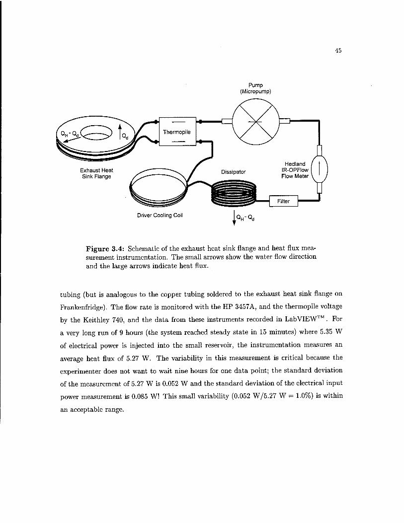
45
Pump (Micropump)
Exhaust Heat Sink Flange
Driver Cooling Coil QH-
Qd
Figure 3.4: Schematic of the exhaust heat sink flange and heat flux mea- surement instrumentation. The small arrows show the water flow direction and the large arrows indicate heat flux.
tubing (but is analogous to the copper tubing soldered to the exhaust heat sink flange on
Prankenfridge). The flow rate is monitored with the HP 3457A, and the thermopile voltage
by the Keithley 740, and the data from these instruments recorded in Lab VIEW™. For
a very long run of 9 hours (the system reached steady state in 15 minutes) where 5.35 W
of electrical power is injected into the small reservoir, the instrumentation measures an
average heat flux of 5.27 W. The variability in this measurement is critical because the
experimenter does not want to wait nine hours for one data point; the standard deviation
of the measurement of 5.27 W is 0.052 W and the standard deviation of the electrical input
power measurement is 0.085 W! This small variability (0.052 W/5.27 W = 1.0%) is within
an acceptable range.

46
3.3. The Data Recording System using Lab VIEW
The software from National Instruments12 called Lab VIEW™ is used to record the
signals read by the HP 3457A and Keithley 740. The LabVIEW™ software runs on a
Pentium™ 100 personal computer with 32 MB of RAM running DOS with Windows 95.
The communication between the two instruments and the computer is accomplished with
GPIB (General Purpose Interface Bus) hardware. To add to the public good, two somewhat
general programs are written by the experimenter in LabVIEW™ to communicate with
the HP3457A and the Keithley 740 — programs that are not specific to the Frankenfridge
application. It is hoped that these so-called "instrument drivers" will be at least useful to
other experimenters in the local laboratory, if not users at different locations.
The program that is specific to the recording of Frankenfridge data requires a small
amount attention here for the use of future experiments and experimenters. The programs
"Frank Rev 2.2" and "Frank Rev 3.0" are well documented in the Show VI Info option
under the Windows menu option. This information is reproduced here.
VI Name: Frank v3.0 This VI takes data from the Frankenfridge device. It assumes
that the HP 3457A Scanning Voltmeter and Keithley 740
Thermocouple Scanner are used to read the sensor package
on Frank in the following way.
HP 3457A Configuration
Channel Connection
0 Flange Mic (Endevco) AC Voltage
1 Driver Accelerometer (Driver) AC Voltage
2 Driver Mic (Endevco) AC Voltage
3 Flange Mic (Endevco) DC Voltage
4 No connection
5 Flow Meter (0PFL0W) Frequency (Hz)
6 Drive Frequency (Hz)
7 Heater load voltage (DC Voltage)
8 Heater load current (DC Current)
9 No connection
Keithley 740 Thermocouple Scanner Configuration
Channel Connection
2 Cold Side Temperature (Type E)
3 Hot Side Temperature (Type E)
4 Thermopile output temperature (Type E)

47
Thermopile intake temperature (Type E)
Thermopile response (mV)
Driver housing temperature (Type E)
Thermal Bath temperature (Type E)
This VI creates (or appends) to a data file with the prefix and
location specified in frame 12. The fields that are written to
this file are outlined below in the order that the columns appear
when the ASCII file is viewed with a viewer (e.g. Notepad) or
imported into a spreadsheet (e.g. Excel).
Field Units
Drive Frequency Hz
Stroke mm
RMS Acoustic Pressure Pa
Pressure Ratio Percent
Acoustic Impedance Ns/m"5
Hot Side Temperature deg C
Cold Side Temperature deg C
Exhaust delta T deg C
Flow Rate g/min
Heat Load W
Exhaust Power W
Acoustic Power W Driver Housing Temp deg C
Bath Temp deg C
T-Pile Discharge deg C
T-Pile Inlet deg C
Time
Date
The Lab VIEW™ programming environment has a very shallow learning curve and
serves the purpose of recording the data of this experiment quite nicely.

Chapter 4.
Measurement Analysis and Results
This chapter analyzes the subsystems that play a large part in the performance mea-
surements and then presents the measurement results. Because the space qualified STAR
resonator has no penetrations for sensor leads and heat exchanger fluids, cooling power and
the temperatures of the stack must be inferred from direct measurements that require no
resonator penetration. The measurement of exhaust heat flux with the exhaust heat sink
flange is used together with the First Law of Thermodynamics to infer the heat pumped
from the refrigerator's cold side. A conduction model of the hot and cold heat exchangers
is created to infer the stack temperatures from the temperatures measured outside of the
resonator at the cold and hot side. First, this chapter will describe how these measure-
ments and inferences are made. Secondly, the results of the measurements are described
and compared to a (linear) DELTAE model. Finally, the Frankenfridge measurement results
are compared to STAR performance.
4.1. Summary of Experiments
The performance of Frankenfridge was measured in eight controlled experiments. The
first three runs were mainly diagnostic in nature to determine that the driver and all of the
measurement systems functioned correctly and that the device behaved as expected at low
amplitudes. Run #4, #5 and #6 produced the most fruitful data. Each was a helium/argon
run and the fridge is operated in the same manner for each of these experiments. First,
the fridge was turned on with no heat load and the cold side was stabilized at 17.2 °C
by adjusting the acoustic pressure amplitude created by the driver. This temperature was
chosen to be just a bit under room temperature to minimize the heat leak from the cold side
to the room. The frequency of the driver piston oscillation was adjusted so that an in-phase
relationshipt between pressure and velocity at the face of the driver piston was maintained.
Once the fridge reached a steady state at the pre-established cold side temperature, the
t The operator monitors a Lissajous pattern on an oscilloscope that is tracing the driver micro- phone and accelerometer signals.

49
electric heat load was activated to dissipate | W at the cold side. The acoustic pressure
is again adjusted to keep the cold side at 17.2 °C. Once this new state is stable (taking
about six to eight minutes) the heat load is again incremented by 1/2 W and the acoustic
pressure is adjusted accordingly to maintain a constant cold resonator temperature. The
operation is continued in this way up to 6.13% pressure ratio in Run #6. See Table 4.1 for
a description of all of the experimental runs.
Because there is significant interest in the time-to-failure of the SETAC drivers, the
total amount of time logged on the driver used in Prankenfridge during these experiments
is 48.6 hours. No driver degradation was detected in the course of these experiments.
4.2. Exhaust Heat Sink Flange
See the section in the Chapter 3 for a detailed discussion about the operation of the
heat sink flange.
The analysis of the exhaust heat sink flange is a straightforward forced convection
treatment.13 A mass flow rate in the hot heat exchanger flange of 660 g/min is used
throughout all of these experiments. The Reynolds number, ReD, for this flow rate is
calculated to be:
ReD = **L = 2576 (4.1) ITflV
where rh is the mass flow rate, \i is the dynamic viscosity of the fluid and D is the inner
diameter of the 1/8 in. (O.D.) copper refrigeration tubing (the inner diameter is measured
to be 0.0625 in.). This Reynolds number is just outside of the laminar flow regime. The
laminar flow regime for flow in pipes is accepted to be 0 ^ ReD ^ 2300 while fully developed
turbulent flow is not found with Reynolds numbers less than 10,000.
The hydrodynamic entry length, that defines the length that it takes the velocity profile
of the flow to become fully developed is,
Xfd,h « 0.05ReD x D = 205 mm (4.2)
Since the total length of 1/8 in. copper refrigeration tubing surrounding the flange is
820 mm, the flow has a fully developed velocity profile for about 75% of the tubing length.
The thermodynamic entry length, that defines the length that it takes the temperature
profile of the flow to become fully developed is,
xfdjt « 0mReDPr xD = 1190 mm (4.3)

50
Table 4.1: Summary of measurements made with Frankenfridge.
Run Date Conditions and Comments
10 Feb. 1997 Mainly a diagnostic check of instrumentation and proof of concept, includes run at lab inaugural. Gas mix is 136 psia, 85.5% He, 14.5% Ar. Cold side is not insulated, exhaust loop instrumentation is not operational. Data recorded and analyzed manually. Run time: 220 min
13 Nov. 1997 Gas mix: 150 psia, 85.5% He, 14.5% Ar. Flow loop instru- mentation operational, check first law balance. Cold side in- sulated, record thermal decay after shut-off for insulation ef- fectiveness. Fix instrumentation snags. Data recorded man- ually. Pressure ratio does not exceed 3%. Diagnostic run. Run time: 240 min
20 Nov. 1997 Gas mix: 157 psia, 85.5% He, 14.5% Ar. Use Lab VIEW™ data recording system. First Law agreement is good at high exhaust power, bad at low. Pressure ratio does not exceed 3.5%. Last diagnostic run. Run time: 280 min
21 Nov. 1997 Gas mix: 151 psia, 85.5% He, 14.5% Ar. Step through heat loads from 0 to 15 W, pressure ratio up to 3.3%. Good data set. Run time: 360 min
8 Dec. 1997 Gas mix: 151 psia, 85.5% He, 14.5% Ar. Check LabVIEW™ modifications and measure bath temperature in attempt to correct low power First Law imbalance. Learned that imbal- ance is not strongly correlated to bath temperature. Com- pletely a duplicate of Run #4. Run time: 120 min
9 Jan. 1998 Gas mix: 155 psia, 85.5% He, 14.5% Ar. Step through heat loads from 0 to 26.5 W, pressure ratio up to 6.2%. Measure driver housing temperature for First Law correction. Good data set. Run time: 660 min
27 Feb. 1998 Gas mix: 156 psia, 85.5% He, 14.5% Ar. This run at 2% pressure ratio is made to compare Frankenfridge performance to STAR performance. Run time: 375 min
3 Mar. 1998 Gas mix: 155 psia, 85.5% He, 14.5% Ar. This run at 3% pressure ratio is made to compare Frankenfridge performance to STAR performance. Run time: 780 min
which means that the temperature profile of the flow is never fully developed in the length
of copper tubing that undergoes heat transfer from the flange. In this expression, Pr is the
Prandtl number, which is the ratio of the momentum and thermal diffusivities; for water
at 300 K the Prandtl number has value of 5.83.

51
Since h, the average convective heat transport coefficient is:
h = ^£ (4.4)
a value for NuD, the average Nusselt number in internal flow, must be calculated. Two
correlations13 for the Nusselt number of flow in the entrance (not fully developed) region,
the Hausen correlation and the Sieder & Täte correlation. The Sieder & Täte correlation
is:
^ = L86f^Vm (4-5) \(L/D)J V/i
where L is the length of the copper tube, /x is the free stream dynamic viscosity and /xs is
the dynamic viscosity at the pipe surface. The ratio of these viscosities is taken to be unity.
This correlation gives a value for the average Nusselt number of 17.5 which leads to a value
of 6760 W/m2 • K for h, the average convection coefficient.
The relationship for the total heat transport from the fluid to the pipe wall is:
Q = hAsATlm (4.6)
where ATlm is the log mean temperature difference and is (AT0-ATi)/(ln(^)). In this log
mean temperature difference, AT0 is the temperature difference of the free stream liquid and
the pipe wall at the outlet of the pipe, and AT{ is the same at the inlet of the pipe. Using
the result of Eq. (4.5) the value for hAa, the equivalent thermal resistance, is calculated
to be 34.0 W/K. This thermal resistance is measured experimentally to be 17.7 W/K.
The measurement of log mean temperature difference was made with the thermopile, a
thermocouple mounted on the inlet to the thermopile and a thermocouple mounted on the
hot heat exchanger flange. The outputs from these sensors were read with the Keithley
740. The measured value is expected to be lower because the calculation assumed that the
whole of the tube is in contact with the flange when in fact, only roughly half of the surface
area of the tube is in thermal contact.
As described in the instrumentation chapter, the measurement system has an absolute
accuracy of 65 mW when a second reservoir is used to add heat in place of Frankenfridge.
However, when the system is used to monitor the exhaust heat flux of Frankenfridge, a 2 W
offset is measured when the refrigerator {i.e., the driver) is not even powered. This offset
is measured because there is a significant temperature difference between the copper heat

52
sink flange and the water in the large thermal bath. Since the water is one to three degrees
Kelvin cooler than the flange, it extracts heat from the flange that does not represent
exhaust heat from the fridge. This offset was not observed in the verification test because
two water baths are used that are initially at the same temperature.
Table 4.2: Subset of data from Run #6 that exhibited a large First Law imbalance
Time Acoustic
Pressure
(Pärms)
Hot Side
Ext. Temp
(°C)
Cold Side
Ext. Temp
(°C)
Exhaust
Temp
Rise
(°C)
Heat
Load
(W)
Exhaust
Heat
Flux
(W)
Acoustic
Input
Power
(W)
Total
Input
Power
(W)
First
Law
Deficit
(W)
11:55 0.0 21.9 22.5 0.043 0.00 2.00 0.00 0.00 2.00
12:46 3182.1 21.9 17.2 0.053 0.00 2.46 0.29 0.29 2.18
13:03 4561.7 22.0 17.3 0.066 0.49 3.03 0.54 1.03 2.00
13:12 5931.7 22.1 17.3 0.083 0.99 3.86 0.92 1.90 1.96
13:25 6941.7 22.2 17.3 0.101 1.48 4.68 1.25 2.74 1.94
13:41 7873.9 22.3 17.3 0.119 2.00 5.49 1.60 3.60 1.89
14:00 8810.3 22.5 17.2 0.134 2.50 6.22 2.00 4.50 1.72
14:22 9624.0 22.6 17.3 0.161 3.00 7.50 2.38 5.38 2.11
14:29 10412.0 22.7 17.2 0.177 3.50 8.12 2.78 6.28 1.84
14:44 11084.0 22.8 17.2 0.192 4.01 8.87 3.15 7.15 1.72
14:54 11814.0 22.9 17.2 0.212 4.50 9.83 3.57 8.07 1.76
15:07 12668.0 23.1 17.2 0.237 5.10 11.01 4.10 9.20 1.81
15:16 13402.0 23.2 17.2 0.257 5.61 11.98 4.58 10.19 1.79
15:22 13974.0 23.3 17.2 0.275 6.12 12.74 4.97 11.09 1.65
15:38 14571.0 23.4 17.3 0.293 6.62 13.66 5.40 12.02 1.64
Some typical data, just after startup, is displayed in Table 4.2. This data came from
Run #6, which is typical of the measurements made for this thesis. In Run #6, the cold
side of the fridge is well insulated and the cold side exterior temperature ("Cold Side Ext.
Temp") is intentionally held fixed at 17.2 °C. With no (or very little) heat leak to the room
(the room is usually about 3 °C colder than the hot side), all of the heat produced by the
resistance heater ("Heat Load") is thermoacoustically pumped to the exhaust flow loop and
measured ("Exhaust Heat Flux"). The column marked "First Law Deficit" is the difference

53
between the total input power and the exhaust heat flux measured in the flow loop. With
this well insulated, "no heat leak" assumption, the First Law restricts this deficit to be zero.
A correction must be applied to the measurement of exhaust heat flux that accounts
for the heat flux associated with the temperature imbalance of the flange and the cooling
water. The simplest correction is to simply subtract the value of exhaust heat flux measured
when the driver is not powered. This initial exhaust heat flux should be zero if the fridge
has been idle for a long period of time (a day) as it was in Run #6. Furthermore, there
is almost an hour between turn-on and the first (zero heat load) data point—this time lets
the fridge settle into steady state at a cold side temperature of 17.2 °C. Subtraction of
this offset from the data results in a much better First Law agreement as shown below in
Table 4.3.
Table 4.3: Subset of data from Run #6 that have been corrected for the First Law imbalance. These are the same data as shown above in Table 4.2
Time Total
Input
Power
(W)
Measured
Exhaust
Power
(W)
Corrected
Exhaust
Power
(W)
Corrected
Deficit
(W)
Relative
Deficit
(%)
11:55 0.00 2.00
12:46 0.29 2.46 0.46 0.18 61.65
13:03 1.03 3.03 1.03 0.00 -0.39
13:12 1.90 3.86 1.86 -0.04 -2.34
13:25 2.74 4.68 2.68 -0.06 -2.19
13:41 3.60 5.49 3.49 -0.11 -3.04
14:00 4.50 6.22 4.22 -0.28 -6.26
14:22 5.38 7.50 5.50 0.11 2.09
14:29 6.28 8.12 6.12 -0.16 -2.62
14:44 7.15 8.87 6.87 -0.28 -3.89
14:54 8.07 9.83 7.83 -0.24 -3.00
15:07 9.20 11.01 9.01 -0.19 -2.09
15:16 10.19 11.98 9.98 -0.21 -2.09
15:22 11.09 12.74 10.74 -0.35 -3.18
15:38 12.02 13.66 11.66 -0.36 -2.99

54
The fact that the corrected deficit grows with increasing exhaust power is suggestive of
a heat leak (this trend would be more apparent if a whole data set were presented here).
The first place to look for such a leak is across the heat sink flange/driver interface. There
is a 0.119 in. thick Delrin™ ring that insulates the large aluminum driver housing from
the resonator, however, it is certain that the thermal resistance of this ring is not very
large. The ring has a 2.00 in. outer radius and a 1.198 in. inner radius with a bolt circle in
between that matches the driver and the flange. The ring could be made thicker to improve
its insulative properties but the corresponding increase in distance between the stack and
the driver is not desirable.
The thermal resistance of the Delrin™ ring is calculated using a standard conduction
analysis that ignores contact resistances. The calculated value (using a contact area of
6.97 x 10~3 m2, a conduction length of 3.2 mm and the thermal conductivity of Teflon™ ,
which is much like Delrin™, as 0.35 W/m ■ K) for the thermal resistance offered by the
insulating ring is 1.3 K/W. The thermal resistance offered by the ring is about 300 times
better than would exist with no ring. By no means is the ring a perfect insulator, rather, at
steady state it will provide enough of a thermal bottleneck to allow a measurable amount
of exhaust heat to gather on heat sink flange and be removed by the circulating water.
The heat flux across the ring between the heat sink and the driver housing is accounted for
in post-processing of the data or on the fly in the Lab VIEW™ system by measuring the
driver housing temperature as well as the hot side flange temperature.
The thermal resistance offered by the insulating ring was measured by monitoring an
E-type thermocouple mounted on the face of the driver housing that contacts the ring and
monitoring the hot side flange temperature. A resistance heater was wrapped around the
driver housing and heated to several elevated temperatures to let the housing absorb heat
to a steady state. After recording several such points, the value of the thermal resistance of
the insulating ring is found to be 1.0 K/W. This is in acceptable agreement with the simple
conduction calculation (1.3 K/W) because an accurate value of the thermal conductivity of
Delrin™ is not known and because the convection mode of heat transfer is not accounted
for in the simple calculation, nor are two-dimensional effects.

55
If the measured value of the thermal resistance of the Delrin™ washer is used to apply
a further correction to the exhaust heat flux measurement, the overall agreement gets a bit
better.
Table 4.4: Subset of data from Run #6 that have been corrected for driver housing heat leak. These are the same data as shown above in Table 4.2
Time Total
Input
Power
(W)
Ring
Temp
Drop
(°C)
Driver
Heat
Leak
(W)
Exhaust
Power
(W)
Exhaust
Plus Heat
Leaked
(W)
New
Deficit
(W)
Relative
Deficit
(%)
11:55 0.00 0.1 0.1
12:46 0.29 0.1 0.1 0.46 0.58 0.29 100.64
13:03 1.03 0.1 0.1 1.03 1.14 0.11 10.34
13:12 1.90 0.0 0.0 1.86 1.86 -0.04 -2.34
13:25 2.74 0.0 0.0 2.68 2.68 -0.06 -2.19
13:41 3.60 0.0 0.0 3.49 3.49 -0.11 -3.04
14:00 4.50 0.0 0.0 4.22 4.22 -0.28 -6.26
14:22 5.38 0.1 0.1 5.50 5.61 0.22 4.15
14:29 6.28 0.1 0.1 6.12 6.23 -0.05 -0.86
14:44 7.15 0.1 0.1 6.87 6.99 -0.17 -2.34
14:54 8.07 0.1 0.1 7.83 7.94 -0.13 -1.62
15:07 9.20 0.1 0.1 9.01 9.06 -0.14 -1.49
15:16 10.19 0.1 0.1 9.98 10.03 -0.16 -1.55
15:22 11.09 0.0 0.0 10.74 10.74 -0.35 -3.18
15:38 12.02 0.1 0.1 11.66 11.72 -0.30 -2.53
The heat leak to the driver is minimized with the help of the driver cooling coil. This
heat exchanger consists of two loops of 1/4 in. copper refrigeration tubing soldered to a
piece of copper shim stock formed into a ring. A hose clamp secures the ring snugly to
the perimeter of the aluminum driver housing. The water that is first circulated around
the exhaust heat sink flange enters the driver cooling coils and absorbs the heat produced
by the driver before being circulated through the large thermal bath. The driver cooling
coil serves dual purposes: one of which is to help dissipate the Joule heating in the voice
coil that threatens to destroy the voice coil windings at high drive currents. The second

56
function of the driver cooling coil is to maintain the driver housing at a temperature much
closer to the temperature of the exhaust heat sink flange, thus minimizing the heat leaked
to the driver housing from the hot heat sink flange. At the highest power operating points,
the temperature difference between the driver housing and the heat sink flange (and thus
across the Delrin™ insulating washer) is only a few degrees Celsius.
The average First Law energy deficit in a range from 0 to 80 W is 450 mW with a
standard deviation of 582 mW. The average relative error (comparing the deficit to the
total input power) is 1.9% in the same range.
It is still bothersome that there is some heat leak from the exhaust heat sink flange to
the room. If the flow loop is monitored for a long time (with no acoustic excitation), nearly
four hours in one measurement, the measured exhaust heat flux never gets below 1.5 W.
4.3. Heat Exchanger Performance Model
In order to compare experimental data to the DELTAE model, knowledge of the stack
end temperatures (hot and cold side) is necessary. Space qualification of the resonator in its
past life required that no penetrations were made in the resonator for signal leads. A simple
mathematical calculation for the parallel thermal resistance of the fins of the heat exchanger
allows the temperature of the central fin region of the heat exchanger to be calculated.
The heat exchangers in Frankenfridge are composed of 50 copper fins (0.254 mm thick)
separated by 0.51 mm. The hot side and cold side temperatures are monitored outside of
the resonator. The hot side thermocouple is located on the copper flange where the hot heat
exchanger is seated and the cold side thermocouple is located just below the cold side heat
exchanger. Between an end of the stack and the corresponding heat exchanger (either hot
or cold) there are at least two paths for heat flow. Conduction from the gas oscillating near
the end of the stack to the fins of the heat exchanger and convection between the same are
two of these paths. The alternating flow convective heat exchange is not well characterized
theoretically. If the heat exchangers are designed properly, the thermal resistance of this
mode is small enough that there is only a small temperature drop associated with the
convection resistance (in DELTAE this drop is only a Kelvin or two at most). The conduction
resistance through the gas is so large that very little heat is transferred in this manner from
the gas to the fins and can be ignored.
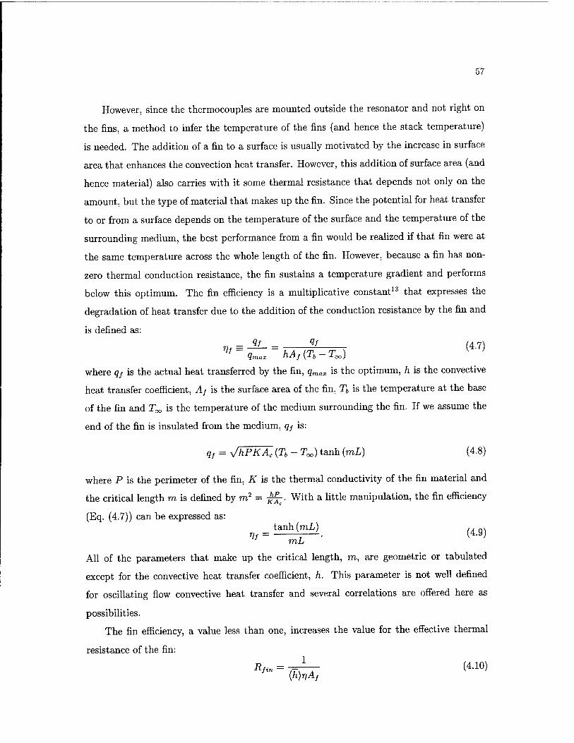
57
However, since the thermocouples are mounted outside the resonator and not right on
the fins, a method to infer the temperature of the fins (and hence the stack temperature)
is needed. The addition of a fin to a surface is usually motivated by the increase in surface
area that enhances the convection heat transfer. However, this addition of surface area (and
hence material) also carries with it some thermal resistance that depends not only on the
amount, but the type of material that makes up the fin. Since the potential for heat transfer
to or from a surface depends on the temperature of the surface and the temperature of the
surrounding medium, the best performance from a fin would be realized if that fin were at
the same temperature across the whole length of the fin. However, because a fin has non-
zero thermal conduction resistance, the fin sustains a temperature gradient and performs
below this optimum. The fin efficiency is a multiplicative constant13 that expresses the
degradation of heat transfer due to the addition of the conduction resistance by the fin and
is defined as:
„, = JL- = q-l (4.7)
where qf is the actual heat transferred by the fin, qmax is the optimum, h is the convective
heat transfer coefficient, Af is the surface area of the fin, Tb is the temperature at the base
of the fin and T^ is the temperature of the medium surrounding the fin. If we assume the
end of the fin is insulated from the medium, qf is:
qf = JhPKAc {Tb - T«,) tanh (mL) (4.8)
where P is the perimeter of the fin, K is the thermal conductivity of the fin material and
the critical length m is defined by m2 = ^. With a little manipulation, the fin efficiency
(Eq. (4.7)) can be expressed as: = tanh (mL) (4 g)
mL
All of the parameters that make up the critical length, m, are geometric or tabulated
except for the convective heat transfer coefficient, h. This parameter is not well defined
for oscillating flow convective heat transfer and several correlations are offered here as
possibilities.
The fin efficiency, a value less than one, increases the value for the effective thermal
resistance of the fin:
Rfin = -J— (4.10) {h)r)Af

58
where Af is the surface area of the fin.
In a paper14 describing the heat exchangers for the TALSR/SETAC device, Garrett
claims that a rough approximation to the convective heat transfer coefficient, hAC, is:
"- = !§ = £ {w)
From the values of the thermophysical properties of the gas mixture shown in Table 1.1,
the simplest model for the convective heat transport predicts hAC — 1020 W/m2K. Since
the flow is oscillating sinusoidally, a root-mean-square average makes sense, and the time
averaged convective heat transport coefficient, (hAC) is 720 W/m2K.
A better approximation to hAC can be calculated if the flow is known to be turbulent
or laminar. The Reynolds number15 is a non-dimensional ratio that compares the inertial
forces of the flow to the viscous forces imposed by a boundary on the flow. For an isolated
flat plate, which like the fins in the heat exchangers except for the fact there is another flat
plate above and below, the Reynolds number is:
Ret = U~AXEX (4.12) v
where AxEX is the fin length along the resonator axis and v is kinematic viscosity. The
flow is turbulent if Reynolds number is large (inertia forces are much greater than viscous
forces) and a low Reynolds number means that the viscous forces are able to restrain the
inertia forces creating a laminar flow. For flow over a flat plate, a Reynolds number of
500,000 marks the transition from laminar to turbulent flow. At the hot heat exchanger in
Frankenfridge, the time averaged sinusoidal free-stream velocity, (IO, is 5.56 m/s for an
acoustic pressure of 30 kPa (see Table 1.1 for gas mixture thermophysical properties). This
leads to a Reynolds number of 6522 which is well below the laminar limit. Likewise, the fins
of the cold side heat exchanger experience average velocity oscillations of 7.93 m/s (with
pressure oscillations of 30 kPa) which leads to a Reynolds number of 3721. The Reynolds
number corresponding to flow in the cold exchanger is a little greater than half the value
at the hot exchanger because although the flow velocity is faster here, the fin length of the
hot exchanger is twice the length of the cold exchanger (see Table 1.1).
The Nusselt number, which can be thought of as the ratio of total heat transfer to
conduction heat transfer, is shown in Eq. (4.13) spatially averaged over a plate of length L:
N^=^ (4-13)

59
where K is the thermal conductivity of the fluid. Scaling arguments15 (similitude) guarantee
that the average Nusselt number is correlated to the Reynolds number and the Prandtl num-
ber (a non-dimensional ratio of the viscous to thermal diffusivity). The standard correlation
for laminar flow is:
^ = NÜ = OMARe^Pr1?3 (4.14) K
The above expression leads easily to the average convective heat transfer coefficient for a
fin in the heat exchanger. The value that corresponds to flow through the hot side heat
exchanger is hH = 700 W/m2K. Since the Nusselt number depends on the square root of
the free-stream flow velocity (see Eq. (4.14)) and this velocity is oscillating sinusoidally, a
time average value of the heat transfer coefficient makes sense. Because the heat transfer
is independent of the sign of velocity, an average over half a period is required.14
1/2 - r (sin x)1/2dx = 0.763 (4.15) 7T Jo
The time average heat transfer coefficient corresponding to the hot side and cold side flow
is shown in Table 4.5. It is comforting to note that these numbers are not substantially
different from the crude calculation shown at the beginning of this section in Eq. (4.11).
With these values of h, the characteristic length, m, can be calculated using values for the
fin cross sectional area and cross sectional perimeter, Ac and Pc, respectively. The results
are shown in Table 4.5.
Now that the heat transfer coefficient has been obtained, only the geometrical aspects
of the exchanger remain to be calculated. Since each fin has different length, the thermal
resistance including the fin efficiency is easily calculated for each fin with a FORTRAN
program or spreadsheet. The symmetry of the cylindrical heat exchanger can be exploited
so that the resistance of each fin in only one-quarter of the exchanger needs to be calculated
on a fin-by-fin basis. Fig. 4.1 shows the geometry of both the hot and cold heat exchanger
(the only difference between the two is that the hot exchanger has fins that are twice as
long in the direction of acoustic flow). In both exchangers, the center-to-center fin spacing,
b is 0.762 mm. The radius of the exchanger, R is 1.9 cm which gives a total number of fins,
iV = 2R/b = 50. By the Pythagorean Theorem, the length of fin n is
Ln = ^(R* - (nb)2) (4.16)

60
d=nb
Figure 4.1: Geometry of the hot and cold heat exchanger, end view of a 1/4 slice.
The total surface area of each fin is twice the depth of the fin, 2xEx times the length
of the fin. The surface area of the edges of the fin is neglected. The thermal resistance
between the fins and the inside of the resonator body of the hot exchanger is calculated in
a spreadsheet to be RH = 0.172 K/W and the cold exchanger Rc = 0.303 K/W. Since the
resonator body is thin copper, it is assumed that there is very little thermal resistance from
the inside of the resonator body to the thermocouple.
Table 4.5: Heat exchanger model summary
Parameter Hot Exchanger Cold Exchanger
Ac 1.62 x 10~6 m2 6.45 x 10~7 m2
Pc 1.32 x 10~2 m 5.59 x 10⁻³ m
(h) 530 W/m2K 1,000 W/m2K
m 104.2 m-1 147.4 m-1
R 0.172 K/W 0.303 K/W

61
4.4. Performance of Frankenfridge
4.4.1. Performance at low amplitudes (PA/P™. < 3%)
Fig. 4.2 shows two graphs: the measured input acoustic power required to attain a
certain pressure ratio inside the resonator and the cooling power for PA/Pm < 3%. In the
presence of a stack and heat exchangers, this acoustic power is responsible for pumping heat
from the side of the stack that gets cold to the side that gets hot.
The DELTAE model is generated by entering each experimental datum point into the
model one at a time and letting the model generate a solution for each point. For the
comparison in Fig. 4.2, the hot and cold side heat exchanger temperatures are targets for
DELTAE and the program is allowed to solve for the input acoustic power and heat pumping
power that correspond to the target temperatures. The pressure at the specific datum
point is also given to DELTAE not as a Guess or Target, but just as an invariant input
parameter. In the same way, the acoustic and heat pumping power is set to be an output
parameter of DELTAE, not a Guess or Target. This allows DELTAE to very accurately model
an experimental condition. The acoustic power required to attain a certain pressure ratio
under the experimental condition is more than 30% greater than DELTAE predicts it to
be. The graph of heat pumping power (or cooling power) shows excellent agreement with
DELTAE at low amplitudes.
4.4.2. Performance at high amplitudes {PA/PW. < 6%)
The high amplitude data from Run #6, where operation up to a 6% pressure ratio was
measured, is presented in Fig. 4.3.
It is reassuring that data from Run #6 below about 4% pressure ratio match data of
Run #4 quite nicely. The offset between measured data and DELTAE in the acoustic power
required to attain some pressure ratio that was evident in the Run #4 data still exists and
is roughly the same—between 30 and 40 percent. The fact that the offset seems to be a very
weak function of pressure amplitude suggests that Frankenfridge possesses some thermovis-
cous loss mechanism not modeled by DELTAE and that the bulk of the discrepancy between
the DELTAE model and measurements is not due to nonlinear effects. This linear effect could
be a dent in the bulb termination of Frankenfridge or some leak or undocumented cavity in-
troduced between the driver, insulating ring, heat sink flange, and resonator interfaces. The

62
100.00
I 10.00 o o. o (A 3 o o < 1.00 4-» 3 a. c
0.10
0.10
100
5. 10 a> o a.
o o ü
0.1
0.10
Run 4, Comparison of Measured Results and DeltaE
1.9585 y = 1.4365x R2 = 0.9999
■ DeltaE Results
♦ Measured Data
y = 1.0597x R2 = 0.9993
1.9016
1.00 Pressure Ratio (%)
10.00
Run 4, Comparison of Measured Results and DeltaE
■ DeltaE Results
♦ Measured Data
1
1.00 Pressure Ratio (%)
10.00
Figure 4.2: Comparison of measured data and DELTAE prediction for PAIPTU < 3%. The outside cold metal temperature is 17.2 °C.
Run #6 data does show a nonlinear degradation in cooling power between the measured
data and the (linear) DELTAE results above a 4% drive ratio. This nonlinear performance
degradation is not so significant as to scare a designer of thermoacoustic engines away from

63
Run 6, Comparison of Measured Results and DeltaE 100.00
I 10.00 a
o o < 3 a c
1.00
0.10 0.10
40,
35
g-30
a>25
£20 01 £15 o Ü 10
5
0
00
00
00
00
00
00
00
00
.00
y=1.4891x19522 ^ ♦ Measured Data ■ DeltaE Model
R2 = 1.0000 ^W"
--
^^?Tl452x1-8805
^^^ R2 = 0.9991
1 ___
1.00 Pressure Ratio (%)
10.00
Run 6, Comparison of Measured Results and DeltaE
-« ■
—i 1 1 1
-- ■ DeltaE Model
♦ Measured Data
--
Hl^T 1 0.00 1.00 2.00 3.00 4.00
Pressure Ratio (%) 5.00 6.00 7.00
Figure 4.3: Comparison of measured data and DELTAE prediction for PA/PTTI < 6%. The outside cold metal temperature is 17.2 °C.
a device that operates above 4% — especially if she is willing to make the small sacrifice in
COP for the substantial increase in power density.

64
4.4.3. DELTAE Model Perturbations
Because this disagreement in acoustic input power between measured performance of
Frankenfridge and the DELTAE is troubling, different physical effects are magnified with new
DELTAE models to uncover clues about the discrepancy. A DELTAE model is created that
includes turbulent flow, another that includes a larger surface area for added thermoviscous
loss and another that uses a different stack geometry that may more closely represent the
rolled Mylar™ and fishing line stack in Frankenfridge.
The thermoacoustic modeling software DELTAE has the capability to model turbulent
acoustic flow; the parameter that DELTAE uses to determine the turbidity of the flow is the
relative roughness. In a duct this is defined15 as the ratio of the surface roughness, e to the
diameter of the duct: rel roughness = e/D. A typical value15 of surface roughness (e) for
drawn tubing is 5 x 10⁻⁶ in.
The result from the DELTAE model with turbulence that is shown in Fig. 4.4 corresponds
to a relative roughness value of 0.1. This value is assigned to the cold reducer, cold duct and
the trumpet but is outrageously large for hardware of the size and type in Frankenfridge.
However, the lip of the trumpet could provide an obstacle to the flow on the order of 10%
of the diameter of the cold duct. While it is not certain that this obstacle could be modeled
as a pipe roughness, it is interesting to see what DELTAE predicts for such a value. At the
least, it sheds some light on the very turbulent limit.
Because the amplitude independent discrepancy of DELTAE predictions and measured
data suggests an inaccurately modeled thermoviscous loss, the surface area of the cold
reducer, cold duct and trumpet is increased by 30% in DELTAE. This new model should
have a lower value for Q and should lessen the difference in the original DELTAE model and
measured data. It does make the discrepancy smaller, but only by a few percent.
Instead of using STKSlab which models a parallel plate stack in DELTAE, a STKREct
is substituted. It is possible that this stack segment will more closely model the Mylar™
film/fishing-string stack used in Frankenfridge. This modification only decreases the dis-
crepancy by a few percent as well. The graphs shown in Fig. 4.4 illustrate these different
models. These data are plotted on a logarithmic axes to highlight any linear deviations from
the unaltered ("Straight") DELTAE results. The fit corresponds to the particular model —
please use the fit in Fig. 4.3 to compare the power law dependence of the different models.

65
Run 6, Comparison of Measured Results and DeltaE 100.00
I 10.00 o o.
o u < 3 o. c
1.00 --
0.10
y = 1.4891x19522 ^ß>
-- + Measured Data
A Turbulent DeltaE (rel rough 0.1)
R = 1.0000^^^^
>£*r^ y = 1 -1284x2036
^^r R2 = 0.9999
1
0.10 1.00 Pressure Ratio (%)
10.00
Run 6, Comparison of Measured Results and DeltaE 100.00
110.00 Q. _o w 3
| 1.00
Q. c
0.10
y = 1.4891x19522 .ggg
+ Measured Data
■ DeltaE with STKREct
R2 = 1.OOOO^gS^^
^^^y = 1.1837x1-8807
^^^ R2 = 0.9992
0.10 1.00 Pressure Ratio (%)
10.00
Figure 4.4: Acoustic power requirements for DELTAE models of Run #6 operating conditions.
The effect of these various model perturbations on cooling power is shown on the graph
in Fig. 4.5. Included on this graph is the measured Run #6 cooling power.
Each one of the model perturbations exhibits the expected behavior—that is, the tur-
bulent flow shows a nonlinear roll-off at about 4% pressure ratio (which agrees well with
the measured data), the addition of thermoviscous damping degrades the cooling power

66
40.00 Run 6, Comparison of Measured Results and DeltaE
3.00 4.00 Pressure Ratio (%)
7.00
Figure 4.5: Cooling power of DELTAE models of Run #6 operating con- ditions.
independently of amplitude (not shown in Fig. 4.5). The change from STKSlab to STKREct
shows a slight increase in cooling power for a given pressure ratio which makes sense since
the fishing line now gets to participate in thermoacoustic heat transport.
In summary, none of these artificial perturbations to the DELTAE model correct the
acoustic power discrepancy, nor do they destroy the excellent agreement of cooling power
for a given pressure ratio below pressure ratios of 3%.

67
4.4.4. Comparison of Frankenfridge Performance with STAR Performance
Data points were recorded on STAR with two gas mixtures, helium/argon and he-
lium/xenon. Run #7 and Run #8, using a helium/argon mix, were made under sim-
ilar conditions and in a similar manner as the STAR data were gathered. The plots
in Figs. 4.6 and 4.7 compare the performance of STAR to the performance of Franken-
fridge at 2% and 3% pressure ratios using coefficient of performance relative to Carnot
(COPR = COP/COPcarnot) as a performance metric.
The operation of Run #7 and Run #8 was different than in the high power runs. The
conditions of Run #7 and Run #8 spanned much larger temperature differences and saw
a lower cooling power to simulate STAR experiments. The fridge was first turned on with
no heat load and a large drive ratio (« 3%) and the cold side cooled to a low temperature
(« -18°C). At this steady condition, a small heat load was applied (« 2 W) and the
cold side temperature allowed to increase. As the cold side temperature increased, the heat
load was reduced by about 20% to 30% to "catch" the cold side temperature and be at
steady state. This procedure eliminates the long exponential approach to steady state (the
experimenter is too impatient and likes to play with knobs and buttons). Since the cold side
temperature is much colder than the room, the heat leak from the room to the cold side
is quite significant. Where in the high power, low AT runs, the exhaust heat sink flange
measurement system was used mainly as a First Law energy check, it is now used to infer
the cold side heat flux (Qc = QBX ~ WAc)-
The performance of Frankenfridge at 2% and 3% show significant deviations from the
DELTAE predictions. This is consistent with the discrepancies in the model and the data of
Runs #4 and #6 shown in Figs. 4.2 and 4.3. Frankenfridge performance in Fig. 4.6 and 4.7
also show significant differences compared to the STAR data at 2% and 3%. This difference
may be due to the fact that the stack position in the standing wave has changed with
the addition of the exhaust heat sink flange and the Delrin™ insulating ring. The flange
moves the stack 0.5 in. away from the driver while the insulating ring moves it another
0.12 in. The STAR driver had a much smaller bellows length than the SETAC driver
used in Frankenfridge which accounts for the largest change in the stack position. This
movement is significant because the classic trade-off between efficiency and heat pumping
power in an engine depends on the product of wavenumber and stack position (kx) in the

68
2% Pressure Ratio Performance Comparison U.AJU -
0.180 • •
• # •
0.160 -
•*■ - 0.140 - A A • A \ £ 0.120 A m
o A ■ £ 0.100 • Ü
£ 0.080 - A
♦»♦ .. \ ♦
■
♦ ^ ■
■ 0.060 - ♦
♦ ■ + Frankenfridge Measured Data
♦J 0.040 • ■ Frankenfridge DeltaE Model
0.020 -
t —I
A STAR He/Ar Measured Data • STAR DeltaE Model
4
♦
0.000 J 1 j 1
0.00 1.00 2.00 3.00 4.00 5.00 Total Cooling Power (W)
6.00 7.00
Figure 4.6: Comparison of COPR at 2% pressure ratio for Frankenfridge, STAR and DELTAE models. STAR data from Ref. 4
0.250
0.200
£ 0.150 - o u
% 0-100
0.050
0.000
3% Pressure Ratio Performance Comparison
• ■■ m
+ Frankenfridge Measured Data
■ Frankenfridge DeltaE Model
A STAR He/Ar Measured Data
• STAR DeltaE Model
♦ ♦ ~ ♦ ♦ ♦ ♦
0.00 2.00
—I 1 1—
4.00 6.00 8.00 Total Cooling Power (W)
10.00 12.00
Figure 4.7: Comparison of COPR at 3% pressure ratio for Frankenfridge, STAR and DELTAE models. STAR data from Ref. 4

69
standing wave for a thermoacoustic refrigerator. The COPR is a monotonically decreasing
function as kx moves away from the driven end of the resonator. See Appendix A for a
short overview of the effect of kx on stack performance and the short stack approximation
to the thermoacoustic heat transport equations. The value of kx for Frankenfridge is about
0.32 and the value for STAR is about 0.28, a significant difference of 14%.By examining
the curves of STAR and Frankenfridge DELTAE model results, one can see that the STAR
DELTAE modelt predicts a larger value of maximum COPR than does the Frankenfridge
model. (Although this appears not to be the case in Fig. 4.6, one only has to extrapolate
the curve of the Frankenfridge model by eye to see that it will not peak as high as the STAR
model.)
4.4.5. Resonator Losses
Comparison of the quality factor of the resonator to the quality factor predicted by the
DELTAE model should reflect the discrepancy in input acoustic power if this discrepancy is
caused by inaccurate modeling of thermoviscous loss.
The quality factor of the resonator is measured by using the driver to introduce a small
acoustic pressure from a constant voltage source (an HP 3562A Dynamic Signal Analyzer,
2-channel). The analyzer makes a sweep of frequency and records the driver microphone
response divided by the driver accelerometer response (but first divides the acceleration by
the angular frequency to obtain velocity). Using the pole and zero values that the analyzer
calculates from a pole-zero curve fit of this impedance (p/v) curve allows a determination
of Q, or the quality factor of the resonance. Using this technique, Q is measured to be 11.0.
The Frankenfridge model in DELTAE can be programmed to produce a frequency sweep
at a very low pressure amplitudes to allow a determination of the model resonator's Q. This
sweep is executed at a constant volume velocity and at such very low pressure amplitudes
that no heat is pumped and no temperature gradient evolves across the stack. A half
power point fit for Q from this pressure response sweep yields a value of 11.75. Using the
relationship of Q to the rate of change of phase angle with frequency (Q = f|j|#]) gives a
t DELTAE did not exist at the time of STAR construction; the model has been constructed as part of this project. The only difference in the STAR model is that kx is smaller than it is the Frankenfridge model.

70
Q of 11.6. The plot of the magnitude and phase of the DELTAE modeled pressure response
appears below.
DeltaE Model Resonance Curve
320.0 325.0 330.0 335.0 340 0 345 0 350 0 355 0 360 0 Frequency(Hz)
Figure 4.8: Acoustic pressure magnitude and phase of the Frankenfridge DELTAE model around the acoustic resonance.
With the stack removed from the resonator of Frankenfridge, the input power required
to attain several pressure ratios was measured. The gas mixture used with no stack is
80.14% helium and 19.86% argon. The results of this experiment are shown in Fig. 4.9 and
compared to two DELTAE models — one that uses INSDUct segments for heat exchangers
(with an augmented perimeter to account for thermoviscous loss on the fins) and one with
HX**** (a finned heat exchanger) segments. The result of both computer models is the
value of acoustic power imparted to the resonator and the input to the model is the same
values for acoustic pressure that were used to experimentally determine the acoustic power
imparted into the physical resonator. The discrepancy seen in Fig. 4.9 between the measured
data and the DELTAE results suggest that there is some part of the resonator that is not
understood, or not modeled in DELTAE correctly.
The quality factor of the physical stackless resonator was measured to be 56. The
models predict that Q to be 66 for the model that has heat exchangers and 83 for the model
with enhanced INSDUcts in place of the heat exchangers.
The fact that Q is larger for the duct model compared to the model with real heat
exchangers is consistent with our understanding of heat exchanger performance because the
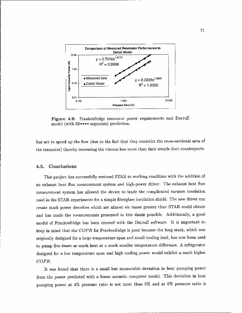
71
Comparison of Measured Resonator Performance to DeltaE Model
10.00
1.00
< 0.10
0.01
y = 0.7016x18779
R2 = 0.9996
y = 0.2226X1 "90
R2= 1.0000
♦ Measured Data
A DeltaE Model
1—
0.100 1.000
Pressure Ratio (%)
10.000
Figure 4.9: Frankenfridge resonator power requirements and DELTAE
model (with HX**** segments) prediction.
fins act to speed up the flow (due to the fact that they constrict the cross-sectional area of
the resonator) thereby increasing the viscous loss more than their simple duct counterparts.
4.5. Conclusions
This project has successfully restored STAR to working condition with the addition of
an exhaust heat flux measurement system and high-power driver. The exhaust heat flux
measurement system has allowed the device to trade the complicated vacuum insulation
used in the STAR experiments for a simple fiberglass insulation shield. The new driver can
create stack power densities which are almost six times greater than STAR could obtain
and has made the measurements presented in this thesis possible. Additionally, a good
model of Frankenfridge has been created with the DELTAE software. It is important to
keep in mind that the COPR for Frankenfridge is poor because the long stack, which was
originally designed for a large temperature span and small cooling load, has now been used
to pump five times as much heat at a much smaller temperature difference. A refrigerator
designed for a low temperature span and high cooling power would exhibit a much higher
COPR.
It was found that there is a small but measurable deviation in heat pumping power
from the power predicted with a linear acoustic computer model. This deviation in heat
pumping power at 4% pressure ratio is not more than 5% and at 6% pressure ratio is

72
about 15%. The correspondingly poorer coefficient-of-performance is small enough not to
deter a thermoacoustic refrigerator designer from designing for high pressure ratio to take
advantage of the dramatically increased power density.
While these experiments have shown excellent agreement with computer models of
the stack, the resonator performance has significant deviations from the DELTAE model.
The computer model predicts the acoustic power requirements to be 2/3 of the measured
acoustic input power needed to reach a certain pressure ratio. This deviation is consistent in
experiments (and the corresponding models) with (Figs. 4.2 and 4.3) and without (Fig. 4.9)
the stack. The discrepancy is greater in the stackless resonator model because the stack is
the dominant loss mechanism and reduces the effect of the resonator model inaccuracy.
The parameter Q, a dimensionless ratio of the amount of energy stored in a resonator
compared to the amount of energy lost per acoustic cycle, is used to compare the model and
the measured results. With the stack and heat exchangers in the resonator, the measured
Q is 11.0 and the Q of the model is 11.7. This agreement is quite good because the loss in
the stack dominates the other thermoviscous losses in the resonator. With the stack out,
the measured Q increases to 56 while the model Q increases to 66. This shows that there is
some thermoviscous resonator loss that is not modeled in DELTAE correctly. In Fig. 4.4 this
discrepancy can be seen to be independent of acoustic amplitude which leads one to believe
that the loss is not a nonlinear one, as turbulence would introduce, but a thermoviscous
loss that is independent of drive amplitude, such as a small leak or gap in the resonator.
It is also possible that this discrepancy in Q is evidence of an energy storage mechanism in
the resonator that is not modeled in DELTAE.
Although there is significant disagreement between the curve of COPR for Franken-
fridge compared to the Frankenfridge DELTAE model, there also exists a large discrepancy
between the STAR data the STAR DELTAE model as shown in Figs. 4.6 and 4.7. The hy-
pothesized thermoviscous loss mechanism not modeled in DELTAE has apparently not been
introduced in the Frankenfridge modification and construction. Indeed, it is possible that
there is a problem with the DELTAE model, or a problem with the way it is used in this
project or even with the software itself (although this last possibility is unlikely—DELTAE
results have been verified on several other occasions.)

73
Further work on this project will be to find the loss mechanism that provides the
disagreement between DELTAE and the measured data. The exhaust heat flux measurement
system will also be examined to correct for the erroneous offset of about 2 W in a more
rigorous way. Since the instrumentation of Frankenfridge has been so successful, it is hoped
that Frankenfridge can be a test bed for research into new stack or heat exchanger designs.

74
References
1. Shelley, M. W., Frankenstein; or, The Modern Prometheus, (London, Lackington and
Co., 1818).
2. Garrett, S. L., Adeff J. A., Hofler, T. J., "Thermoacoustic Refrigerator for Space
Applications," AAIA J. Thermophys. Heat Trans. 7, 595-599 (1993).
3. Baluster, S. C, McKelvey, D. J., "Shipboard Electronics Thermoacoustic Cooler,"
Master of Science Thesis, Physics Department, Naval Postgraduate School, (1995).
DTIC Report No. ADA 300514; U.S. Patent No. 5,647,216 (Jul. 15, 1997).
4. Adeff J. A., Garrett, S. L., Hofler, T. J. "Measurement of the Space Thermoacous-
tic Refrigerator Performance," Master of Science Thesis, Physics Department, Naval
Postgraduate School, (1990). DTIC Report No. AD A241-320.
5. Moran, M. J., Shapiro, H. N. Fundamentals of Engineering Thermodynamics, 2nd Ed.
(Wiley k Sons, New York, 1992).
6. Wheatley, J. C, Swift, G. W., Migliori, A., "The Natural Engine," Los Alamos Sci-
ence. 14, (1986).
7. Swift, G. W., "Thermoacoustic Engines," J. Acous. Soc. Am. 84, 1145-1180 (1988).
8. Ward, W. C. and Swift, G. W., Design Environment for Low Amplitude Thermoacous-
tic Engines, Version 3.04b. (Software available from Energy Science and Technology
Center, U. S. DOE, Oak Ridge, Tennessee, http://rott.esa.lanl.gov).
9. Ward, W. C, Swift, G. W. DELTAE Tutorial and Users Guide, Version 2.0. (Los Alamos
National Laboratory, LA-CC-93-8, Sept. 1995).
10. Swift, G. W. "Thermoacoustic Engines and Refrigerators," Encyclopedia of Applied
Physics, Vol. 21 (Wiley k Sons, New York, 1997), pp. 245-264.
11. Rüssel, R. A., "Energy Analysis of the Thermoacoustic Life Science Refrigerator,"
Master of Science Thesis, Physics Department, Naval Postgraduate School, (1994).
12. LabVIEW™ Full Development System Version 4.1, National Instruments Corpora-
tion, Austin, TX, 1997.
13. Incropera, F. P., DeWitt, D. P., Fundamentals of Heat and Mass Transfer, 3rd Ed.
(Wiley k Sons, New York, 1990).

75
14. Garrett, S. L., "Thermoacoustics Life Sciences Refrigerator: Heat Exchanger Design
and Performance Prediction", June (1992); Garrett, S. L., Perkins, D. K., Gopinath,
A., "Thermoacoustic Refrigerator Heat Exchangers: Design, Analysis and Fabrica-
tion," Heat Transfer 1994 Proc. 10th International Heat Trans. Conf. 4, 375-380
(1994).
15. Fox, R. W., McDonald, A. T., Introduction to Fluid Mechanics 4th Ed. (Wiley &
Sons, New York, 1992).

Appendix A.
Effects of Stack Position on Engine Performance
The complicated equations that predict thermoacoustic heat transport given in the
explanation of DELTAE in Chapter 2, or found in Swift's 1988 paper (Ref. 7) are much too
cumbersome to easily understand. However, a much simpler set of equations can be written
if the thermoacoustic stack is considered to be parallel plates that are very short compared
to the acoustic wavelength and that this stack is short compared to the distance that the
stack is positioned from the rigid end of the resonator. A short stack7 allows the magnitude
of acoustic pressure and velocity oscillations to be considered constant throughout the
stack which simplifies the equations dramatically. Further, if the viscosity of the gas is
ignored, there is no dependence of fluid velocity in the direction normal to the stack plates
(perpendicular to the acoustic flow).
A sound wave not near a boundary is largely adiabatic, which means that a parcel
of the medium (assumed to be compressible ideal gas in this development) experiences a
temperature change as it is expanded and compressed. The term, "parcel of gas" refers to
a small element of gas that is composed of many molecules so that a macroscopic treatment
of the element can be applied, but the element is small enough that the material properties
and acoustic variables may be treated as constant within the element. The temperature
change of a parcel of gas is related to the pressure change with the following expression:
Using a Maxwell relation, along with the fact that the inverse of specific volume is the
density (- = p) this expression can be written as:
where s is the entropy per unit mass of the gas parcel. By the standard properties of partial
derivatives, Eq. (A.2) can be written as,

77
which allows convenient substitution of the isobaric coefficient of thermal expansion when
the expansion coefficient is expressed as ß = — ^(ffOp-
The First Law of Thermodynamics can be written as:
5Q = SU + 6W {AM)
Tmds = cpdT - vdp (AAb)
where cp is the gas specific heat at constant pressure and v is specific volume. If this
expression of the First Law is considered for a constant pressure process, the second term
on the right vanishes and:
—^ =^ (A5) ds J p cp
which can substitute nicely into Eq. (A3) to give:
Ti = — (A6) PmCp
For fluid that can thermally communicate with the stack, the heat per unit volume of
the fluid that is transferred perpendicular to the direction of acoustic flow is pmcpST, where
6T is the change in fluid temperature due to the flow of heat. The volume velocity of the
fluid that is considered to be thermally active is U6KUi where II is the perimeter of the
stack measured transversely to the acoustic flow direction, SK is the thermal penetration
depth (see Eq. (2.6)) and ux is the acoustic velocity magnitude. The product of these two
quantities (the change in heat per unit volume and the volume velocity of thermally active
fluid) is the thermoacoustic heat flux given below:
Q ~ USKulPmcpÖT (A.7)
From a picture like the one in Fig. 2.4 in Chapter 2, one can see that
/ VT \ ST = 27\ - 2x1VT = T, 1- ^— (A8)
where VT is the temperature gradient along the stack and Xi is the peak acoustic displace-
ment.
The critical gradient, as defined in Eq. (2.7) is the value of VT that makes 5T = 0. In
the short stack approximation, the critical gradient is
VTcHt = - (A9)

78
If we call T the ratio of VT/VTcri( and combine Eqs. (A.7) and (A8) we get:
Q ~ mKTmßPlUl (r -1) (Aio)
This expression points out that when T < 1 heat flows against the temperature gradient as
in a refrigerator. When T > 1 heat flows "downhill" and the device operates as a prime
mover. When T = 1 heat does not flow and the cycle does no useful work.
The work flux is estimated by considering the volume change experienced by a parcel
of gas as it translates an acoustic displacement and is acted on by the acoustic pressure.
This volume change is expressed as
Y = ßST (All)
where V is the total volume of gas that is thermodynamically active and is equal to U5KAx.
In this expression, Ax is the length of the stack. The work flux, in general, is piSVu and
by combining Eqs. (A6), (A8), (AIO) and Eq. (All) we can express the work flux as
W^nsJ^-pluAxiT-l) (A12) PmC-p
If we employ another thermodynamic relation, 7 - 1 = Tmf a where 7 is the polytropic
coefficient, or the ratio of the specific heat of an ideal gas at constant pressure to the specific
heat at constant volume, and a is the speed of sound. Using this equality we can recast the
work flux in a more convenient form for ideal gases:
W~IWB(7-1) —(r-l)*Aa: (A13)
where the wavenumber, k, is equal to u/a. In the short stack approximation, both heat
and work flux are quadratic in the acoustic pressure or velocity and both heat and work
flux change sign as T passes through unity.
As discussed in Chapter 2, the efficiency or COP of an engine relates the heat flux to
the work flux. In a refrigerator, the COP is
COP = -S- (A14) W
into which we can substitute our new expressions for heat and work flux to obtain Eq. (A 15).
The COP will be regarded as an equality even though the above expressions for heat and
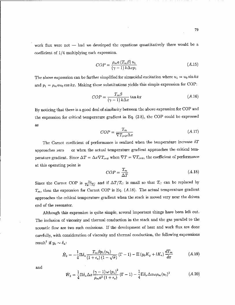
79
work flux were not — had we developed the equations quantitatively there would be a
coefficient of 1/4 multiplying each expression.
COP = f"a(^)Ml (A15) (7 — 1) kAxpi
The above expression can be further simplified for sinusoidal excitation where ui = u0 sin kx
and pi = pmau0 coskx. Making these substitutions yields this simple expression for COP:
COP = , T"f, A tan kx (A16) (7 — 1) KAX
By noticing that there is a good deal of similarity between the above expression for COP and
the expression for critical temperature gradient in Eq. (2.8), the COP could be expressed
as
COP=V£K-X {AA7)
The Carnot coefficient of performance is realized when the temperature increase 5T
approaches zero — or when the actual temperature gradient approaches the critical tem-
perature gradient. Since AT = AxVTcrit when VT = VTcrit, the coefficient of performance
at this operating point is
COP=^ (A18)
Since the Carnot COP is j^f^ and if AT/TC is small so that Tc can be replaced by
Tm, then the expression for Carnot COP is Eq. (A18). The actual temperature gradient
approaches the critical temperature gradient when the stack is moved very near the driven
end of the resonator.
Although this expression is quite simple, several important things have been left out.
The inclusion of viscosity and thermal conduction in the stack and the gas parallel to the
acoustic flow are two such omissions. If the development of heat and work flux are done
carefully, with consideration of viscosity and thermal conduction, the following expressions
result7 if y0 ~ 6K:
* - -?■"-(!+Toa-U)(r" ° -n{y°K'+lK-] £ (A19)
and 2
w2 = j-nW7 l]^Pl\ (r -1) - \mvAxuPm{uxf (A20) 4 pma2 (1 + es) 4

80
0.45 Maximum Stack Performance
i i i i i
0.4 /^ ^^^\
QO.35 / ^\^
O ^^^^
0.3
n in i i i i i
0.05
x10
0.1 0.15 0.2 0.25 Stack Location, kx
0.3 0.35
0.15 0.2 0.25 Stack Location, kx
0.35
Figure A.l: Stack performance as a function of stack position in the standing wave
Eq. (A. 19) is an expression for the enthalpy, or total energy flux, which is the sum of the
heat and work flux, or, H2 = Q2 + W2. Indeed, Eq. (A. 19) looks much like our Q except
that it has some extra terms in the denominator, a specific heat correction (es) for the
stack material and the square root of the Prandtl number (a). The second term, the one
that subtracts energy from the first term, represents the heat loss due to conduction in
the stack and the gas in the direction parallel to acoustic propagation. The fact that the
enthalpy and work flux variables have a subscript 2 signifies that they are second order in
the acoustic variables, pi and Ui, which are first order. Just like the expanded enthalpy
equation, the work flux equation, Eq. (A.20) has an extra term that represents the extra
viscous loss caused by the stack.

81
Using these equations, an idea of the effect that kx has on efficiency and heat pumping
power can be quantitatively explored. Fig. A.l illustrates that as the stack is moved away
from the driven end of a refrigerator, the COP relative to Carnot comes to a peak at
some small distance from the driver and then decreases monotonically. When the stack is
right against the driver face the magnitude of the pressure oscillations is very large and
consequently the stack temperature span is large. This large temperature span causes the
thermal conduction "down" the stack to decrease the COPR. As the stack moves away from
the driven end into the "sweet spot" that gives highest COPR, the refrigerator is pumping
very little heat and the actual temperature gradient is very close to the critical temperature
gradient. (In fact, the idea of critical temperature gradient as a single number is not true in
the presence of viscosity. It really spans a range of values, sort of a "no man's land" where
the device is neither a refrigerator nor a heat pump.)
To be able to pump more heat, the stack must be moved into a region where the
velocity amplitudes are greater, which implies larger viscous losses in the stack. Although
the COP gets larger for increasing stack position (kx), the Carnot COP goes to infinity as
the magnitude of the pressure oscillations go to zero at the pressure node (because the stack
temperature difference, AT, approaches zero). This increase in Carnot COP is larger than
the increase in COP for a given increase in kx which makes the ratio of COPR decrease.
The lower plot in Fig. A.l shows that the stack can pump more heat as the stack moves
away from the driven end.
Because the stack in Frankenfridge is not at all short, according to our criterion, a
shorter stack length was used to create the graphs in Fig. A.l. In addition, some of the
values for gas mixture thermophysical parameters are not the values that are accurate
for the Frankenfridge device. Although the values used in this exercise are realistic, the
purpose is to point out the dependence of stack performance on the position of the stack in
the standing wave.
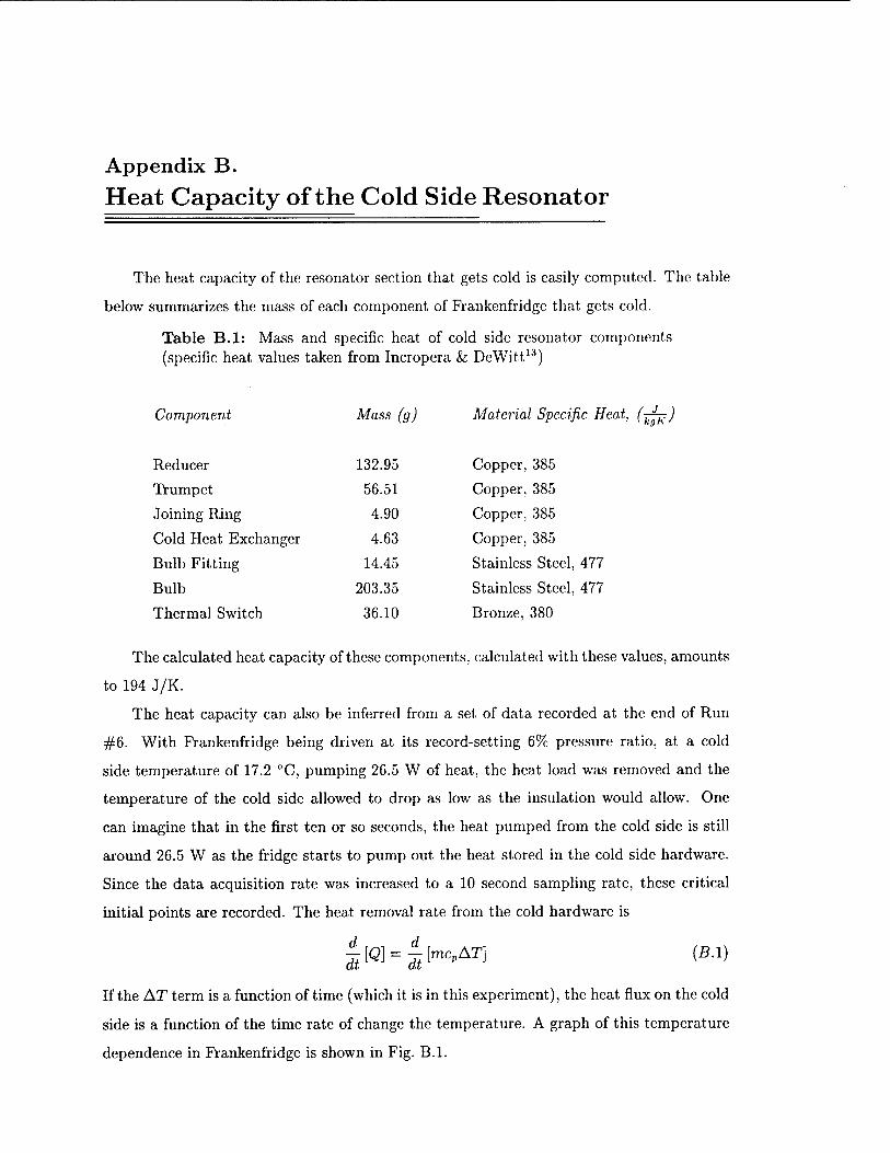
Appendix B.
Heat Capacity of the Cold Side Resonator
The heat capacity of the resonator section that gets cold is easily computed. The table
below summarizes the mass of each component of Frankenfridge that gets cold.
Table B.l: Mass and specific heat of cold side resonator components (specific heat values taken from Incropera & DeWitt13)
Component Mass (
Reducer 132.95
Trumpet 56.51
Joining Ring 4.90
Cold Heat Exchanger 4.63
Bulb Fitting 14.45
Bulb 203.35
Thermal Switch 36.10
Material Specific Heat, (-pr-) kgK
Copper, 385
Copper, 385
Copper, 385
Copper, 385
Stainless Steel, 477
Stainless Steel, 477
Bronze, 380
The calculated heat capacity of these components, calculated with these values, amounts
to 194 J/K.
The heat capacity can also be inferred from a set of data recorded at the end of Run
#6. With Frankenfridge being driven at its record-setting 6% pressure ratio, at a cold
side temperature of 17.2 °C, pumping 26.5 W of heat, the heat load was removed and the
temperature of the cold side allowed to drop as low as the insulation would allow. One
can imagine that in the first ten or so seconds, the heat pumped from the cold side is still
around 26.5 W as the fridge starts to pump out the heat stored in the cold side hardware.
Since the data acquisition rate was increased to a 10 second sampling rate, these critical
initial points are recorded. The heat removal rate from the cold hardware is
> = |K,Ar] (B.l)
If the AT term is a function of time (which it is in this experiment), the heat flux on the cold
side is a function of the time rate of change the temperature. A graph of this temperature
dependence in Frankenfridge is shown in Fig. B.l.

83
2.0
0.0
Initial Temperature Drop, Run 6, First Three Points
30 Time Elapsed (s)
50 60
Figure B.l: Graph of the initial temperature drop in Run #6.
If the heat flux is taken to be 26.5 W during this 60 seconds, then the heat capacity of
the cold side hardware can be inferred. Taking the magnitude of ^ to be 0.18 ± 0.02 °C/s
yields a value for heat capacity of 145 J/K which is comparable to the calculated value (the
calculated value is 34% larger).

Appendix C.
Manufacturer Specifications of Sensors
This appendix includes the manufacturers specifications of the sensors used in Franken-
fridge. Unfortunately, the exact serial numbers of the Entran accelerometer and Endevco
microphone that are inside of the driver are not known (without breaking the driver apart).
For these sensors, the generic specification sheet is included.
Also included in this section is information about the PR100 preamplifier for the piezore-
sistive strain gauge sensors. These amplifiers were made in the lab in May of 1997.
The pages in this appendix are numbered consecutively with the body of the thesis.

85
Piezoresistive Pressure Transducer
Model 8510B-200, -500 and -2000 • 200 to 2000 psi, 300 mV Full Scale • Rugged, Miniature
DESCRIPTION The ENDEVCO" Model 85 1013 is a rugged, miniature. high sensitivity piezoresistive pressure transducer. It has a 10-32 mounting thread, d. 15 inch '3.8 mini race diam- eter and is available in ranges from i r-si to 2111 ill psi. Its high sensitimry combined withresonance makes it ideal for measuring dynamic pressure.
ENDEVCO pressure transducers feature a rbur-acnve arm strain gage bridge diffused into a unique sculptured silicon diaphragm for maximum sensitivity and wideband frequency response. Self-contained hybrid temperature compensation provides stable performance over the temperature range of o°F to 2uO°F '-18=C to +93°C). ENDEVCO transducers ai<o feature excellent linearity (even to 3X range;, high shock resistance, and negligible sensitivity to temperature transients.
The Model 8510B is designed for a wide variety of aerospace, automotive and industrial measurements which require a combination of smaii size, high sensitiv- ity, and wideband frequency response. Its vent tube may be connected to a standard reference manifold or used for differential pressure measurements.
The Model 851 OB is available with Metric M5X0.8 mounting thread as 8510B-XXM5 on special order.
ENDEVCO Model 106/109 Dual Channel System. Model 4430A Signal Conditioner, or Model 68207 3CAS" Computer Controlled System are recommended as signal conditioner and power suppiy.
SPECIFICATIONS CERTIFIED PERFORMANCE: All specifications assume +75;F (+24:C) and 10 Vdc excitation unless otherwise stated. The following parameters are 100% tested. Calibration data, traceaole to the National Institute of Standards and Technology (NIST1. is supplied.
Model Units 8510B-2OO -500 -2000
RANGE [1] psig 0-200 0-500 0-2000
ENDEVC MODEL 851 OB
POSITIVE SENSITIVITY [2) mVrosi 1.5 ±0.5 COMBINED: NON-UNEARITY. NON-REPEATABIUTY. PRESSURE HYSTERESIS (3] % FSO RSS Max 0.50 Non-Uneafity. Independent % FSO Typ 0.25 Non-Repeatability % FSO Typ 0.1 Pressure Hysteresis % FSO Typ 0.1 ZERO MEASURAND OUTPUT [3] mVMax r10 ZERO SHIFT AFTER 3X RANGE ±% 3X FSO Max 0.2 THERMAL ZERO SHIFT From 0°F to 20O°F (-18°C to <-93°C) THERMAL SENSITIVITY SHIFT From 0"F to 200°F (-18°C to +93°C)
CMEGGITT AEROSPACE ENDEVCO
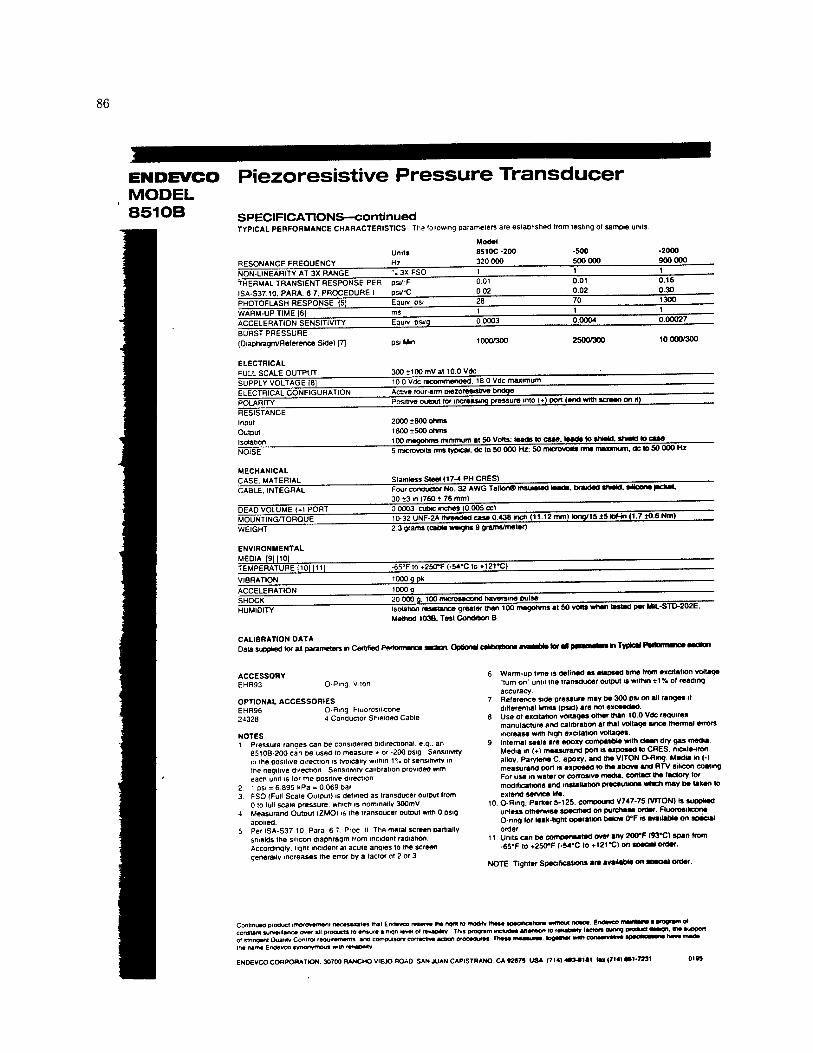
86
ENDEVCO MODEL 851 OB
Piezoresistive Pressure Transducer
SPECIFICATIONS—continued TYPICAL PERFORMANCE CHARACTERISTICS The following parameters are established Irom testing ol sample units.
RESONANCE FREQUENCY
Units
Hz
Model 8510C -200 320 000
-500 500 000
-2000 900 000
NON-LINEARITY AT 3X RANGE °.3X FSO 1 1 1
THERMAL TRANSIENT RESPONSE PER
ISA-S37.10. PARA. 6.7. PROCEDURE 1
psirF
PSl/'C
0.01 0 02
0.01
0.02
0.16 0.30
PHOTOFLASH RESPONSE fS]
WARM-UP TIME [6|
28 70 1300
ms 1 1 1
ACCELERATION SENSITIVITY EQUIV. psvg 00003 0.0004 0.00027
BURST PRESSURE [Diaphragm/Reference Side) [7]
ELECTRICAL FULL SCALE OUTPUT
psi Mm 1000/300
300 tlOOmVat 10.0 Vdc
2500/300 10000/300
SUPPLY VOLTAGE [81 10 0 Vdc recommended. 18 0 Vdc maximum
ELECTRICAL CONFIGURATION Active tour-arm piezoresistive bridge
POLARITY Positive output tor increasing pressure into (-1 ■) port (end with screen on it)
RESISTANCE Input Output Isolation
NOISE
2000 ±800 ohms 1600 1500 ohms 100 megohms minimum it 50 Volts; leads lo case, lead» to shield, shield to case 5 microvolts rms typical, dc to 50 000 Hz; 50 microvolt» rms maximum, dc »SO 000 Hz
MECHANICAL CASE. MATERIAL CABLE. INTEGRAL
DEAD VOLUME (»I PORT MOUNTING/TORQUE
Stainless Steel (17-4 PHCRES) Four conductor No. 32 AWG Teflon® insulated leads, braided shield, sikcone jacket
30 ±3 in (760 t 76 mm) 0 0O03 cube menes (0.005 cc) 10-32 UNF-2A threaded case 0.438 inch (11.12 mm) long/15 ±5IDI-in (1.7 ±0.6 Nm)
2.3 grams (cable weighs 9 grams/meter)
ENVIRONMENTAL
MEDIA [91 [101 TEMPERATURE |10||11|
VIBRATION
ACCELERATION
HUMIDITY
-65'F to *250*F (-54°Cto+121'C)
1000 gpk
1000a 20 000 g. 100 microsecond haversine pulse soiauon resstance greater than 100 megohms at SO volts when tested per MIL-STD-202E.
Method 103B. Test Condition B
CALIBRATION DATA Data supplied (or all parameters ai Certified Performance sseson. Optional ca*braoone In Typical F^jiluiinano» eacton
ACCESSORY EHR93 O-Ping. Viion
OPTIONAL ACCESSORIES EHR96 O-Ring Fiuorosilicone 24328 4 Conductor Shielded Cable
NOTES 1 Pressure ranoes can be consiaered bidirectional e.g . an
8510B-200 can be used to measure * or -200 DSig. Sensitivity in the positive direction is rvDicaily within l°.o ot sensitivity in the negitive direction. Sensitivity calibration provided with each unit is for me positive direction
2. 1 OS! = 6 895 kPa = 0.069 bar 3. FSO (Full Scale Output) is defined as transducer output from
0 to lull scale pressure, which is nominally 300mV 4 Measurand Output (ZMO) is the transducer output with 0 psig
applied. 5 Per ISA-S37.10. Para.6 7. Proc. M The metal screen partially
shields the silicon diaphragm from incident radiation Accordingly, light incident at acute angles to me screen generally increases the error by a factor ot 2 or 3.
6 Warm-up time is defined as elapsed time Irom excitation voltage "lum on" until me transducer output is wiihm r1% of reading accuracy.
7 Reference side pressure may be 300 psi on all ranges if differential limits ipsid) are not exceeded.
8 Use ot excitation voltages other than 10 0 Vdc reouires manufacture and calibration at that voltage since mennal errors increase with high excitation voltages.
9 Internal seals are eooxy compatible with dean dry gas media Media in (♦) measurand port is exposed lo CRES. nickle-iron alloy. Parylene C. epoxy. and the VITON O-fling Media in (-) measurand port is exposed to the above and RTV silicon coating For use in water or corrosive meek», contact the factory tor modifications and installation precaution» which may be taken to
extend service lite. 10 O-Ring. Parker 5-125. compound V747-75 (VITON) Is suppked
unless otherwise specified on purchase order. Fiuorosilicone O-nng tor leak-tight operation below 0"F is available on special
order. 11 Units can be compensated over any 200*F (93*C) span from
-65°F to *250°F (-54-C to +121*C) on specs» order.
NOTE: Tighter Specifications are available on aoaoai order.
ConMiuao oroduci imorovamam necassitai»* mal Enoavco TOOT» ma mjM lo mod*» met« «pecmcal«»» wimcM no«». Endavco ■"—*»"» * w>»r«n <* conn*» lurvwunc« ovof au Dtooura to «rnura a nign KY« ol rwaonv Th.s rxooram nduoM «lamon ra lafcaoam/ tacnra owing proouneiaian. »■» «man ol stnnoant Oualitv Comroi reouiramams ano compulsory corraeflv» acoon orocoouraa that« maaawea. ngainar wan c lha nama Enoavco synonymous wiin n
ENDEVCO CORPORATION. 30700 HAWCHO VIEJO ROAD SAN JUAN CAPISTRANO CA 92675 USA (7l4)4aXM1»t tax (714H»1-7a31

87
PRESSURE TRANSDUCER TEST REPORT MODEL 85103-200 SERIAL # 10063
Range Sensitivity Excitation Zero Pressure Output Full Scale Output Non-Lineanty Hysteresis Non-Repeatability Combined Lin., Hyst., & Rep." Thermal Zero Shift Zero Shift After 3 X FSO Thermal Sensitivity Shift Input Resistance Output Resistance Isolation Resistance
•RSS
200 psig 1.45 mV/psi
10.00 Vdc 4 mV
290 mV .09 %FSO .03 %FSO .03 %FSO
_ * %FSO .31 %FSO .01%3XFSO . 14 %
1690 n 1526 n >100 MCJ
-1.5
NON-LINEARITY 0
(% FSO)
-1.5
-5
□rat "= 2'e -'aceaoie to '-9 National institute ot Stanaaräs and Technology and in accordance wttn ,.,IL-S~D-45662A.
THERMAL ZERO SHIFT
(% FSO)
-5
^5
THERMAL SENSITIVITY
SHIFT (%)
-5
80 100 % FSO
200
150 200 DATE 21 JUN 96
31j © V "ft
EMEGGITT AEROSPACE
30700 RANCHO VIEJO ROAD. SAN —AN CAPISTRANO. CA. 9267S USA (714) 493-8181 FAX (714) 661-7231 Form 26707/8

Model 8514-10, -20 and -50 • 10 to 50 psi, 300 mV Full Scale • Rugged, Subminiature • 0.065 Inch Diameter
X DESCRIPTION The ENDEVCO' Model 8514 is a rugged, submmia cure piezoresiscive pressure transducer. It has a case diameter ot'onlv 0.065 inch (1.65 mm: and is available in ranges from 10 to 5o psi mil scaie. Full scale output is 300 mV with high overload capabil- irv and high frequency response.
ENDEVCO pressure transducers feature an active four-arm strain gage bridge diffused into a sculp- tured silicon diaphragm for maximum sensitivity and wideband frequency response, Seif-contained hybrid temperature compensation provides stable performance over the wide temperature ranee of o°F to 200°F H8°C t° -t-^.va. ENDEVCO transducers also feature excellent lineanrv leven to 3X range;, high shock resistance, and high stability during temperature transients.
The Model 8514 can be installed in locations which are difficult to reach. Its smaii size permits tlush mounting on curved surfaces, its high sensitivity combined with small size and high resonance makes the Model 8514 suitable for use on smail-scale models in wind tunneis.
ENDEVCO Model 106/109 Dual Channel System. Model 4430A Signal Conditioner, or Model 68207 BCASrM Computer Controlled Systems are recom- mended is signal condinoner and power supply.
ENDEVCC MODEL 8514
MOUNTING DCTAIt
STANDARD TOLERANCE INCHES i MILLIMETERS)
XX. »'■ 03 (X-— Si XXX - *• 010 I XX ■ ..- 251
SPECIFICATIONS CERTIFIED PERFORMANCE: All specifications assume *75:F l*2-TC) and 10 Vdc excitation unless otherwise stated. The following parameters are 100% tested. Calibration aata. traceaoie to me National institute ol Standards and Technology (NIST). Is supplied.
Model Units B514-10 -20 -50
RANGE |1] DSio 0-10 0-20 ° - » POSITIVE SENSITIVITY [11 30 ± 10 COMBINED: NON-LINEARITY. NON-REPEATABIUTY. PRESSURE HYSTERESIS [2] •■. FSO RSS Max 1.0 Non-Uneenty. Independent % FSO Typ 0.50 Non-flepeataoility "4 FSO Typ 0 1 Preeeufe Hysteresis % FSO Typ 01 ZERO MEASURANO OUTPUT |3) ZERO SHIFT AFTER 3X RANGE THERMAL ZERO SHIFT From 0*F to200°F(-16°Cto*93''C) THERMAL SENSITIVITY SHIFT From 0-F to 200"F (-18*C to *93°C)
i ". 3X FSO Max : 10
0.1
15 t 5
0.50 0.25 0.1 0.1 t 10 0.1
612
0.50 0.25 0.1 0.1 ± 10 0.1
c MEGGtTT AEROSPACE

89
ENDEVCO MODEL 8514
Piezoresistive Pressure Transducer
SPECIFICATIONS—continued TYPICAL PERFORMANCE CHARACTERISTICS: The following parameters are established Irom testing of sample units.
Model Units 8514-10 -20
RESONANCE FREQUENCY Hz 140 000 180 000 NON-LINEARITY AT 3X RANGE i 3X FSO THERMAL TRANSIENT RESPONSE PER psi/'F ISA-S37.10, PARA. 6.7. PROCEDURE 114) psi/°C
1.0
-50 320 000
PHOTOFLASH RESPONSE. [51
0.001 0.002
WARM-UP TIME [6] ACCELERATION SENSITIVITY Longitudinal Lateral BURST PRESSURE (Diaphragm/Reference Sidel
ELECTRICAL FULL SCALE OUTPUT SUPPLY VOLTAGE [5) ELECTRICAL CONFIGURATION POLARITY RESISTANCE Input Output Isolation NOISE
MECHANICAL CASE. MATERIAL CABLE, INTEGRAL
DEAD VOLUME (+) PORT MOUNTING
WEIGHT (excluding lead wiresi
ENVIRONMENTAL MEDIA
TEMPERATURE [71 VIBRATION ACCELERATION
Equiv. psi
0.003 0.005
0.005 0.009
Equiv. psi/g Equiv. psi/g
0.00015 0.00006
0.0002 0.00005
0.0O03 0.0002
psiMin
300 ±100 mV at 10.0 Vdc
200/25
10.0 Vdc recommended. 18 Vdc maximum Active tour-arm piezoresistive bridge Positive output tor increasing pressure into (♦) port (end with semen on it)
1800 ±800 ohms 1600 ±500 ohms 100 megohms minimum at 50 Volts; leads to case, toad« lo shield, shield 10 case 5 microvolts rms typical, dc to 50 000 Hz; 50 microvolts rms maximum, dc lo 50 000 Hz
Nickel - Iron Alloy Four leadwires No. 36 AWG solid copper conductor. FEP Teflon« insulated 30 ±3 in. (760 ±76 mm) 0.000015 cubic inches (0.0002 cc) Bond into #50 drill hole (1.78 mm) using an RTV. such as DOW CORNING RTV is not permitted within 0.10 Inch (2.5 mm) of unit1 s face 0.08 gram (Leadwires weigh 0.9 grams/meter. Sleeved leadwiree weigh 2 grams/meter)
Internal seals are epoxy and are compatible with clean dry gas media. Ilioln In (+) measurand port is exposed to nickel-iron alloy. Parytene C. and «poxy. For use in or corrosive media, contact the factory tor modification» and installation pracauoona which may be taken to extend service life -65°F to +250^ (-54-C to +121°C) 1000 gpk
20 000 q, 100 microsecond havetsine pulse Isolation resistance greater than 100 megohms at 50 vote, par MIL-STD-202E. Method 103B. Test Condition B. External case is seated with epoxy. Circuit wühtncai through tube, is coated with Parytene C
CALIBRATION DATA Data supplied for ail parameters in Certified F^rformance section. Optional casbrabor» available lor an r. • in Typical
OPTIONAL ACCESSORIES 25011-1 LeadwireRed 25011-2 Leaowire Black 25011-3 Leadwire White 25011 -4 Leaowire Green
NOTES 1. 1 psi = 6.895 kPa = 0.069 bar. 2. FSO (Full Scale Output) is defined as transducer output
change Irom 0 osig to + full scale pressure. Calibration provided is tor positive pressure.
3. Zero Measurand Output (ZMO) is the transducer output with 0 psig applied.
4. Use of excitation voltages other than 10.0 Vdc requires manufacture and calibration at that voltage since thermal errors increase with high excitation voltages.
5. Per ISA-S37.10. Para 6.7. Procedure II. 6. Warm-up time is defined as elapsed time from excitation
voltage "turn on" until the transducer output a within ±1% ol reading accuracy.
7. Units can be compensated over any 200°F (93°C) span from -65°F to +250°F (-54°C to +121"C).
NOTE: Tighter specifications are available on special order
Continued product improvement necessitates mat Endevco reseive the right to modify mesa specttications without nonce. Endevco mamtara a program of constant surveillance over ail products to ensure a nigh level ot reliability. This program includes attention lo reliaMey Moors during product design, me sup, ol stnngent Qualify Control requirements, ana compulsory corrective action procedure. Those measures, together weh consaivativ« apsancabona have made the name Endevco synonymous with rii—rewv.
ENDEVCO CORPORATION. 3070O RAHCMO VIEJO ROAD. SAN JUAN CAPISTRANO. CA 92A7S USA (714) «Milt tan (714) 681-7231 0195

90
Entran
"OFF-THE-SHELF" STOCK PROGRAM
EGA-125 Series Miniature Accelerometers
• 5g TO 5000g RANGES • TO 250 mV FULL SCALE • VARIETY OF MOUNTINGS - SMALL SIZE & WEIGHT • STEADY STATE AND DYNAMIC RESPONSE
Entran's EGA-125 Series accelerometers are a state of the art achievement in miniature accelerometer design. Developed with the user in mind, the EGA otters an optimum combination ot characteristics which permit acceleration, vibration and shock measurements where small size and mass are ol prime importance.
The EGA's rugged construction eliminates the fragility nor- mally associated with miniature accelerometers. Entran's EGA is ottered in a variety ot mounting styles to allow ease ol handling and mounting. This mounting versatility is well suited to meet most requirements Irom aerospace to indus- trial usage and is available at no extra charge. 0.7cr damping is also available as an option.
The EGA-125 is a piezoresistive accelerometer which com-
bines a tulty active semiconductor Wheatstone bridge with the technology of sensor design. Its high output enables the EGA to dnve most recorders and data monitoring systems directly, without amplification or costly signal conditioning. The semiconductor circuitry is tuHy compensated for temper- ature changes in the environment and possesses excellent thermal characteristics.
The EGA-125 is functional from steady state to high dynamic responses and is ranged for "g" loads which are commonly experienced in research, testing, and control Available in "g" ranges from 5g to 5000g. Entran's EGA miniature accelerometer is well suited for a myriad ot applications from aerospace to consumer industries. Typical applications vary in scope Irom flutter testing to wind tunnel models to vibratory and shock disturbances in industrial testing.
Entran Specification EGAS-1870

91
SPECIFICATIONS
MODEL EGA-125 -5
EGA-125 -10
EGA-125 -25
EGA-125 -50
EGA-125 -100
EGA-125 -250
SfiA-124 -500
EGA-125 -1000
tfiA-125 -2500
EGA-125 -5000
RANGE ±5g ±10g ±25g ±50g ±100g ±250g ±500g ±1000g ±2500g ±5000g
"OVERRANGE ±25g ±50g ±125g ±250g ±500g ±1250g ±2500g ±3000g ±5000g ±10000g
SENS. mV/g nom. 15 12 5 4 2.5 1 0.5 0.25 0.1 0.05
" RES. FREQ. nom. 300 Hz 500 Hz 1000 Hz 1200 Hz 1500 Hz 2000 Hz 3000 Hz 4000 Hz 6000 Hz 8000 Hz
"OFF-THE-SHELF" STOCK IN EGA-125-10D. -100D. -250D AND -1000D AND EGA-125F-10D, -100D AND -250D
DAMPED VERSIONS.
NON-LINEARITY ±1%
TRANSVERSE SENS. 3°t max
THERMAL ZERO ±I%FS;IOO°F
THERMAL SENS. ±2,A%/100"F
WEIGHT Vi gram nom (w/o leads)
INPUT IMPEDANCE nom. lOOOQtyp.: 2000Qoptional (500Smin.) with 900Q output
OUTPUT IMPEDANCE nom. .„_. 900Q optional ,auu- with 2000B input
EXCITATION «
15VDC
COMPENSATED TEMP. ^O'FtaUO'FRI'CtoT/'Q OPTION T: WF to 140*F
IO"C » eo*o
OPERATING TEMP. s
-40'Fto250'F(-40'Cto12rQ
1 Useful frequency ranae s 20% ol Resonant Fiequencv. ! Overranoe ior use within 30% ol Resonant Frequency. 3 Available with 0.7a damping to mcrem usehj rang* as nigh as 50% ol resonance with overrange at all treouenctes (see Bulletin EGDAMP). 4 Zero otlsel ol 115mV typ. at 80*F aller warm-up. Lower values avertable on reauest. s ± 2'.5%F S. / lOO'F lor 5g Model. 8 Other Excitations and Temoerature Ranges available on request.
EGA-1 25
.140 (356) ^
140 T t
(3 561 '
24
1610) "
|460)
Sal
AWG 34-7/42 Telton Insulated Leads -
z Compensation Module 0.16 dia max x 1% nom (4mm dia. max x 32 nom.)
dlm:lnche>8 (dlnvmm)
1 RED
Compensation Modulo
OPTION '75" 5 WIRE OUTPUT FOR ZERO OFFSET ADJUST + Output is split into 2 wires, Green and Blue.
GREEN t + 0UT user connects a 25fl potentiometer across Green and Blue with center tap
BLACK as + 0UtPut- " '" Example: EGA-125/5-
' WHITE
_• - IN -• - OUT
OPTIONAL MOUNTING STYLES
(69fJ_
135 I |3 43Q_
( T :©
EGA-125R-
"IT- u7T
.135 ' (3.4)
_ 145 (3 7)> -»-4 W (3 7)
» yu*>A in (6.9) (94~
EGA-12SF-
Sltcllklttlll llk|Kt It

92

93
1 IR-OPFLOW FLOW METERS INSTALLATION & MAINTENANCE
INSTRUCTIONS
IMPORTANT: READ INSTRUCTIONS THOROUGHLY BEFORE INSTALLING FLOW METER
DESCRIPTION
A. GENERAL The lR-OPF;ow is an axiai Daocie wneei :urcme rype flow meter cased on :ne Deitcn wneei cnnci- pai. This unioue Datentea aesign maKes :r.e iR- OPFiow a very accurate, reoeataoie. :near device. No: cniy is tne lR-CPF:ow crease, cut it is aiso a rugged, trcuoie-free fiow meter wmcn can be usea in a wide variety of inaustnes including: meaicai. cnarmaceutical. cnemicai Drocessing, DUID & pacer, ana many otners.
5. PRINCIPLE OF OPERATION Fluid flows througn the meter C first cassing rhrougn a neiicai nozzle <1; wmcn causes now to spiral, rotating in a neiicai oartern. The soiranng fluid then imoacts on the flat blaae rotor vii. caus- ing the rotor to soin. The rotor is aesignea to immediately aeveioo a rotation-mauceo fnction- free fluid bearing, tnus eliminating any potential bearing wear.
An infra^rea. eiectro-ooticai transmitter and receiver 0is molded into the DOOV of the meter, along with a pair of miniature circuit boards, pro- viding voitage stabilizers ano automatic IR outDut
level control that automatically compensates for varying fluid opacity levels*, providing a souare wave electronic output signal.
This design inherently bleeas off entrained gas. improving the accuracy of the meter. It also elimi- nates the need for flow straignteners or special lengths of inlet piping to stabilize turbulent flow. This compact meter can be installed in any orien- tation, immediately adjacent to 90° elbows or other fixtures, upstream or downstream, giving you greater system design flexibility, as well as saving time and money during installation.
*Clear. transparent and translucent fluids, must transmit infrared light
2. MATERIAL CHARACTERISTICS OF PVDF (Polyvinylidene Floride)
A. MATERIAL OF CONSTRUCTION Trade name — Kynar**
All wetted parts of the IR-OPF!ow are PVDF. excluding the O-ring. Wetted parts include any part of the meter that will or could come in contact with the fluid.
List of wetted parts: 1. Barbed fittings 2. Flow meter body 3. Rotor 4. Helical nozzle
5. End caps 6. Strainer 7. Bearings
(Viton O-ring seals.)
B. CHEMICAL COMPOSITION OF PVDF Polyvinylidene fluoride is a fluropolymer consist- ing of three basic materials (caroon, hydrogen and florine).
CHEMICAL COMPATIBILITY OF PVDF For a complete list of compatible fluids consult either Hedland or
Soltex Polymer Corporation 3333 Richmond Ave. P.O. Box 27328 Houston. TX 77227 (713)522-1781
'(Registered Trademark of Pennwalt Corporation)

94
D. EFFECTS OF VARIOUS FLUIDS ON PVDF ". WeaK Acias - no erfect. 2. Strong Acids - attacxeo bv fuming suifunc 3.
nitric acias at nign temoeratures. 3. WeaK Alkalies - no erfect. -i. Strong Alkalies - no erfect. 5. Organic Solvents - Resistant :o most. Siiant
attacK DV some, imonttiea by seme amines. keystone, and estners. (Reference ComDass Corrosion Guide II)
OPERATING PARAMETERS
A. TEMPERATURE RANGE iFric arc Amoient) Dew Point to +185 degrees F, Dew Point to +85 degrees C.
Since the iR-OP Flow nasDrinteacrcjitc-oarcs "noioeo into trie body ot :ne meter it s strcngiy recommended that 185 degrees "anrenneit not be exceeded. Exceeding 185 - F can cause irreparaoie damage to tne circuit boarcs.
3. FLOW RANGES The iR-OPF!ow is avaiiaDie in six afferent sizes .vnicn cover a flow range trom .22 - 22 GP.M.
Specific Flow Ranoes: 502-101 .03 - .53 GPM (0.1 - 2 L?M) 502-102 .08 - 2.38 GPMf0.3 - 3 L?M) 502-103 .13 - 3.96 GPM 10.5 - "5 LPM) 502-104 .26 - 7.93 GPM (1.0 -20 LPM) 502-105 .79-19.81 GPM I3.0-75 LPM) 502-106 1.32 - 23.02 GPM (5.0 -125 LPM)
Consult factory with srjecific aDDlications reouir- ing an extended flow ranges. "Warning," over spin may permanently damage the flow meters.
:. RECOMMENDED VISCOSITY RANGE - 1-5 cSt (without correction) The effects of changing viscosity on the IR- OPFlow are the same as any other turoine flow meter. It is imDortant to rememoer that a turbine flow meter is a viscosity deDendent device where as the viscosity increases tne linearity of the flow meter will decrease. (Water-line fluids are ideally suited for use with the lR-OPFIow.) The IR-OPFlow is calibrated with water.
CORRECTION PROCEDURE FOR HIGHER VISCOSITIES For viscosities greater than 5 cSt consult the factory. The IR-OP Flow can be useo on fluids greater than 5 cSt, however, the K-Factor (lin- earity) will change. This reouires a recaiibration of the IR-OP Flow at the known viscosiry to determine the new K-Factor.
D. RECOMMENDED FILTRATION
Meter Micron Filtration Mesh Filter 502-101 35 micrometer 400 mesn
'502-102 50 micrometer 300 mesn '502-103 100 micrometer 80 mesn '502-104 100 micrometer 80 mesn '502-105 100 micrometer 80 mesn '502-106 100 micrometer 80 mesn
IR-OPF!ow sizes 2-6 are fitted with strainers to helD Drotect against dirt, fiber, ano other contam- inants. Due to space restriction, it is not oossioie to fit size 1 with a strainer. Removal of the strainer will reduce pressure droo througn the flow meter, ano may also cnange the linearity of the meter. Removal could also suPiect the meter to solid contaminant wnicn couio damage the meter.
'The strainer is a 30 mesn filter/550 micrometer.
E. CLEANING
1 STEAM CLEANING Sleam sterilization is not possible with the IR-OPFlow due to the hign temperature of the steam. Steam sterilization will perman- ently damage the flow meters Deanngs ano printed circuit boards.
2. CHEMICAL CLEANING Chemical cleaning the IR-OPFlow is per- missable provided the chemicals are com- patible with PVDF (poiyvinylide fluoride).
F. BI-DIRECTIONAL FLOW The IR-OPFlow is designed to only provide fluid readings in the forward flow direction only. Reverse flow will not unoully restrict fluid flow.
INFRA-RED SENSOR
wrme
brown (signal)
green — (screened cable)
SUPPLY VOLTAGE 5-15 VDc (6-33 mA) Do not exceed 15 VDc. Doing so can cause over-heating and the eventual failure of the PC boards. Printed circuit boards are non-repairable.

95
3. FREQUENCY OUTPUT E*ciuainqMoa..»502-'24 50212« 1 502-128. Consult factory tar lurtnar aetans on :nni moows.)
1. Sauare wave oulse. unscaiea 2. Output impeaance 75 onms 3. Directly prooorttonal to flow rate 4. Output - Dc freauency 5. Offset .64 voits 6. Peak voltage = Supply voltage - 1.2';':
(example: 12Vdc - 1.2V = 10.3V) 7. Peak to peak voltaae = Sucoiy voitage -
1.2V-.64V: (example: 12Vdc - 1.2V - 54V = -i0.16V)
3. Output signal cycle 66.7% «example: at 100 Hz there is a 6 miilisecona on time, ana a 4 millisecond off time.
9. TTL/CMOS circuit comparability The lR-OPFiow nas an operational amcufier outDut wnicn nas a nign mout imceaance ana a ;ow output impeaance.
2. FREQUENCY RANGES FOR IR-OPFLOW K Factor
Moaei Freauencv (H21 -ulses/Gai. 502-101 60-1200 136.250 502-102 40-1200 2C.2S0 502-103 27-300 12.112 502-104 20-600 -1.542 502-105 25-625 -.703 502-106 21-521 552
2. CABLE REQUIREMENT 1. 20 - 22 AWG (American Wire Gauge! 2. 3 conductor-snieia cable
NOTE: Avoid influences of strong electro- magnetic forces as they can carriage components on the PC beard.
INSTALLING THE IR-OPFLOW IN THE FLUID LINE
Strainer a
SS5
Mod« | Numoer i
Connection»!) Thread Sizes
Dimensions (Inertes) |
A B C I
502-101 I Bare Fitting lor .27" ID Hose 0.4 1 1.6 0.3 |
502-1021 3aro Fitting tor .35" 10 Hose 3.5 1.3 14 1
502-103 I Baro Firtino tor .47" ID Hose 0.5 1 1.3 0.5 1
502-104 I 3aro Fittina tor .63" ID Hose 0.6 2.3 0.6 1
502-105 1 1" Maie NPTV BSP .55 ■■ 3.15 ■77 |
502-1061 1" Male NPT/BSP 65 3.15 95 |
E.
Make sure the fluid is compatible with PVDF (polyvmylidene fluoride) and meets viscosity, pressure, and temperature parameters of the iR- OPFIow. The fluid must also meet filtration requirements as listed in 3.D.
Install the IR-OPFlow in the fluid line with the arrow pointing in the direction of flow. All IR- OPFIows are supplied with barbed hose fittings as standard equipment. If the IR-OPFlow is to be placea in a metallic fluid line, optional 316 Stain- less Steel fittings available for sizes 1 - 4. Consult factory for price and availability.
While installing thelR-OPFlow in the fluid line oe careful not to over torque the ena caos or otner fittings on the flow meter. Due to the soft compo- sition of PVDF the booy or threaas can be per- manently distorted.
Attach wires to the readout display with the ais- play and power off. Not oniy wiil this help to avoid a potential snock hazara. but it can also helD prevent an error in hooking the flow meter to an incorrect 115VAc supply
If additional cable is required to hookup the flow meter to a digital display take caution when sol- dering to ensure correct connections.
Connect digital display to power supply and enter scaling factors for both the rate and total. Follow the manufacturers instructions for pro- gramming digital display.
The IR-OPFlow is now ready for use.
•SFor other fittings, consult factory
To] r~
°p&Pi Hi*] I 1
*6>
® %

96
'«rating mnovann
.01 ""1
■* i :M««- —
i so««o« C^ASS :o.'j I
^
arm KM«U n '•o a anew» it
TROUBLESHOOTING
A. if the reaaout aoes not orovice correct informa- tion, review tne scaling factors ana the numoers programmea.
3. Next checK :ne wiring ncoKuDs to :ne cisDiay ana ail soiaer points.
C. Finally cnecK the flow meter rcr contamination.
D. Consuit Healand for additional assistance.
REPAIRING THE IR-OPFLOW
A. Replaceable Darts for the lR-CPF:ow 1. Barbea Fittings 2. Viton O-rings 3. End CaDS 4. Strainers (Consult factory for price ano avaiiabiiity.i
3. Non-repairaDle pans for lR-OPFiow 1. Rotor 2. Bearings 3. Printed circuit boards
3. LIMITED WARRANTY
The Hedland Division of Racine Federated. Inc. warrants to the original purcnaser. for the Denoa of one year from the date of purcnase. that eacn new flow meter is free from defects in materials ana worxmansnip.
The warranty does not cover meters that have been camaged due to abuse, incorrect installation, cr operated beyono Hedland's stated maximum para- meters for the IR-OPFIow.
Heolana's sole obligations under the warranty is imitea to the reoair or replacement of parts, deter- mine to be defective after inspection by Hedlana. Reoair or replacement of parts at Hedland's discre- tion.
Healand is not liable for any conseauential damages or any contingent liabilities arising out of the failure of any flow meter part component part or accessory.
The above warranty supersedes and is in lieu of ail other warranties, either expressed or implied ano ail other obligations or liabilities. No agent, representa- tive or distributor has any authority to alter the terms of this warranty, in any way.
IR-OPFLOW BARB FITTING DIMENSIONS iin mcresi
Mod« | A (Size) | DIa.
3 Dia.
C Dia. Dia.
E Oia.
F Dia. 1 G H I J K L M N 0
Dia.
-01 .380 | 202 | 230 I 240 226 267 1 V60 1.005 807 .609 .41 V .333 .150 .066 .150
-02 .668 =28 1 430 310 288 342 1 -.427 1.228 1.03 .832 634. .503 .195 .079 228
-03 I 556 519 I 460 422 -92 462 1 1.450 1.112 920 .723 .536 .437 .156 .064 .306
-04 | 900 530 I 610 515 532 £37 I '594 1.322 1.069 .753 493 .185 .071 460
-05 1.165 1.014 | 340 - :n 772 I 2.096 1.750 1.453 1.156 .899 .700 .234 .104 .616
-06 1.181 1.026 .915 397 .964 2.132 1.730 ♦'20 1.470 1210 1.000 .675 .238 .121 .770
nn DIVISION OF RACINE FEDERATED INC
MAIUHQ ADDHE3S PO. BOX140S RACINE Wl 53401 TELMPHOMt: (414)039-4770 oM-800-HEDlANO
SHIPPING AOOMSS: 2200 SOUTH STREET RACINE. Wl 53404 FACSnmj: (414)639-22e7 or 1-800-CHK-FLOW FORM M34A1/92

97
PlEZORESISTIVE SENSOR PRE-AMPLIFIER AND SIGNAL CONDITIONER PR100
OPERATIONS GUIDE
1 4 Direct AC Gain AC Direct DC Output
© © 0 7 100 10 1000 +
2 5 Low Pass Filter Polarity
© Norm © Reverse © 8
3.2 kHz Ofl 32 kHz
3 6 9 AC Output Sensor DC Output
© © ©
Power Direct
@ 10 Output AC Direct DC AC Gain
© © © 100 10 1000
Voltage +
© 11 Adjust
© 12
0 0
DC Output
©
Polarity Low Pass Filter
Norm © Reverse ©
3.2kHz Ofl 32kHz
Sensor AC Output
© ©
Figure 1
THE FRONT PANEL:
The front panel shown in Figure 1 can be divided into three sections. The left and right wings contain the outputs, inputs and controls for each channel while the center of the panel contains the power LED and the bias supply control and monitor sockets.
The circuit and function for the left and right pre-amp channels are identical, as is the front panel interface. The sensor input socket is a Switchcraft "TINIQG" 4-pin. The pin-out used in this device is shown below. So that the device can be immediately usable upon receipt, two Switchcraft plugs (the mate to the TINI QG) are included. It is very important that these plugs be wired to the sensor in accordance with the pin-out below! The figure below (Figure 2) is drawn as though the user is looking at the front panel.

98
Front Panel View
1: Signal (-), white
2: Bias (+5Vdc), red
3: Signal (+), green
4 Bias (-5Vdc), black
Figure 2
BIAS SUPPLY:
The center of the front panel contains the bias supply interface and the power on indicator LED (number 10 on the drawing.) Using the 20 turn potentiometer (11) the bias supply can be tweaked between 9.6 VDC and 10.5 VDc. This bias voltage can be monitored with a multimeter via the banana plug receptacles (12). The bias supply circuitry provides a very stable supply and while it is good practice to check the supply voltage before making a series of measurements, the supply does not generally need to be adjusted.
AC SIGNAL MODE:
The PR 100 can amplify and condition two AC signals - one signal per channel. Use switch 4 to select AC signal input for the left channel. There are three amplifier gain settings, 10, 100 and 1000 -- use switch 1 to set the AC gain. Included in the AC amplification circuit is a choice of two low pass filter cut-off frequencies, 3.2kHz and 32 kHz. Use switch 2 to set the cut-off frequency, or disable the filter altogether (the OFF position.) To invert the amplified and optionally filtered AC signal, use the Polarity switch, switch 5.
Obviously, if switch 4 is set for AC signal inputs, the active output terminal is the isolated BNC receptacle 3, labeled AC output.
The AC amplifier circuit uses an AD620 instrumentation amplifier chip. The specs for this chip from Analog Devices are included at the end of this brief. The gain-bandwidth product for the AD620 chip is 800 kHz at a gain of 10, 120 kHz at a gain of 100 and 12 kHz at a gain of 1000. This means that at the highest gain setting, the response will roll off at 12 kHz, even if the filter switch is set to 32 kHz.

99
DC SIGNAL MODE:
Since piezoresistive sensors are often used for static measurements, like strain gauges, a DC output mode is included. The gain amplification switch is inactive in DC mode as is the Low Pass Filter switch. The polarity switch is active, however. Use the isolated DC Output BNC receptacle (receptacle 9) to monitor the DC mode.
The DC mode circuitry employs an AMP03 differential amplifier chip which is a unity gain high input impedance output chip. This chip is used so that a voltmeter or other measurement device will not directly load the sensor. The chip also serves to isolate the ground reference of the signal from house ground. Documentation on this chip is also included.
DIRECT MODE:
The direct signal mode allows the user to monitor the sensor signal directly and through no signal conditioning or amplification. Use the two non-isolated BNC terminals (receptacles 7 and 8) to monitor this signal. Remember that the shield of these BNC terminals is not a reference (as the shield is the reference in AC and DC mode) - the center pin of the BNC 7 is referenced to the center pin of BNC 8. The shields of BNC plugs 7 and 8 are connected to the chassis (and in turn connected to house ground.)
The direct mode option is included for users who may want to use their own differential amplifier. The user should be aware that the device attached to the direct output terminals (BNC 7 and 8) could provide a significant impedance load to the sensor which could skew measurement results.
TROUBLE SHOOTING:
The circuit schematic is included in this brief- however, the actual circuit board layout is not. The circuit board layout is easy to understand by comparing the schematic and the board layout and knowing the following things:
. The board layout sort of models the front panel - that is, the bias supply circuitry is in the center of the board and the left channel is to the left, etc.
. The AC circuitry for each channel is toward the bottom of the board (so the left AC channel is to the bottom left corner nearest the blue edge connector as you look down from above the box with the front panel facing you) and the DC circuitry is directly above the AC circuits. Since the board is connected to the front panel via a removable edge connector- board removal is simply a matter of removing three screws and unplugging the board from the edge connector.
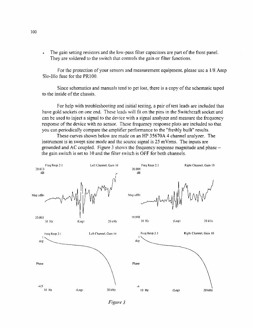
100
The gain setting resistors and the low-pass filter capacitors are part of the front panel. They are soldered to the switch that controls the gain or filter functions.
For the protection of your sensors and measurement equipment, please use a 1/8 Amp Slo-BlofuseforthePR100.
Since schematics and manuals tend to get lost, there is a copy of the schematic taped to the inside of the chassis.
For help with troubleshooting and initial testing, a pair of test leads are included that have gold sockets on one end. These leads will fit on the pins in the Switchcraft socket and can be used to inject a signal to the device with a signal analyzer and measure the frequency response of the device with no sensor. These frequency response plots are included so that you can periodically compare the amplifier performance to the "freshly built" results.
These curves shown below are made on an HP 35670A 4 channel analyzer. The instrument is in swept sine mode and the source signal is 25 mVrms. The inputs are grounded and AC coupled. Figure 3 shows the frequency response magnitude and phase — the gain switch is set to 10 and the filter switch is OFF for both channels.
Freq Resp 2:1 Lett Channel. Gain 10 20.013
dB
Mag (dB)
Freq Resp 2:1 Rieht Channel. Gain 10
20.003 10 Hz (LOE)
20.008 dB
Mae (dB)
19.998 20 kHz 10 Hz (Log) 20 kHz
Freq Resp 2:1 Left Channel. Gain 10 Freq Resp 2:1 Right Channel. Gain 10
Phase Phase
-4.5 10 Hz (Log) 20 kHz 10 Hz (Log) 20 kHz
Figure 3

101
Freq Resp 2:1 Left Channel. Gain 10 Freq Resp 2:1 Right Channel, Gain 10
dB- dB-
Mag (dB) Maa (dB)
10 Hz (Log) 20 kHz 10 Hz (Log) 20 kHz
Freq Resp 2:1 Left Channel, Gain 10 1
des
Freq Resp 2:1 Right Channel, Gain 10 1
des
Phase Phase
-90 -90
10 Hz (Log) 20 kHz 10 Hz (Log) 20 kHz
Figure 4
Figure 4 shows the frequency response functions for each channel in the gain 10 setting but with the 3.2 kHz filter switched on. Upon receipt of the device, it would be a good idea to try to reproduce these graphs and check the other gain and filter settings. If there are significant discrepancies, something is probably wrong-please don't hesitate to get in touch with me.

102 I i K^/l I ill'1!.,.
/ l)l,l< Mill \IS P.dge Card Connections (Bridec .Sensor Dual Amn)
1
2
! Yrllnw<»<mi«|
Bluclw/vcllowl
YHmW<W/fM|tn4f|
lunclion 1 UN lb. AC AmplLeftl
('I IN to. A( Ampdrftl
HIN Tot DC Amp lieft)
Ein A
B
C
Wire Yellow
Function GamrtewaloctLeftl
! PufplelwJ vrHow) I'tlNfot IK' Ampll eftl D
E
BkK AC Amp OUTPUT f left)
; t g
Pur«*
Gtcr
DC Amp OUTPUT II «HI
Po-et Suftprv Common
1 • | » 000 Votll
F
H
1
K
Yellow UaMReimortl.efll
II L
M
N
While 111 A<kw» PM (1 to V|
12 Black 11 s ooo Vom II 14 1! 16 ir ii n 20
Gfecti
r,.n Yellow (»(Mut)
Dluf <w/vtUowl
Putntelw/yrlhiwl
tjrrjr
Blue
Co,
(')J!0Vo»Po«. Wiper
Power SunpJr Ccmramm
( ) IN fat AC Amp IRj«MI
IMINfat AC Amplltittal
IMINIotDCAmp(lti|hl|
Power Sire** Cm—UUP
DC Aire>UUIPUTIIlipml
Power Srrppr* Cnmipua
T
K
S
T
U
V
w X
V
Black
Yellow
Ycrmwlw/anrpic)
Yellow
Bbct
»a.
l-IAetpMPMIlttVI
Gem Rewwor tAiftrto
(MN far DC Am. lieft)
Gam »awwo» (Rift«)
DC Amp OUTPUT Ob»* 1
IM: VniPrrweeJuppt,
OUVolPOWBtopptT