IJRCS Vol. 1, No. 3, 2021, pp. 226-243 ISSN

IJRCS International Journal of Robotics and Control Systems

Vol. 1, No. 3, 2021, pp. 226-243 ISSN 2775-2658

http://pubs2.ascee.org/index.php/ijrcs

https://doi.org/10.31763/ijrcs.v1i3.351 [email protected]

An Adaptive Sliding Mode Control for Single Machine Infinite Bus System under Unknown Uncertainties

Magdi S. Mahmoud 1*, Ali Alameer 2, Mutaz M. Hamdan 3 Systems Engineering Department, King Fahd University of Petroleum & Minerals, P. O. Box 5067, Dhahran 31261,

Saudi Arabia 1 [email protected]; 2 [email protected]; 3 [email protected]

* Corresponding Author

1. Introduction

Large disturbances in power systems are difficult to precisely model and may require imposing unrealistic assumptions when modeling them. Their significant inherent uncertainty mainly causes the difficulty. This study investigates a nonlinear model of Single Machine Infinite Bus System (SMIBS), and we design an advanced robust control law that guarantees asymptotic stability under bounded unknown uncertainties to handle those exacting conditions. Before discussing some of the proposed control laws in the literature, we first give an overview of modeling Synchronous Machines (SM) in general. In the literature, different SM nonlinear models with different orders are considered, mainly depending on the study's objectives. We observed that a general nonlinear dynamic model is deliberated by Kundur in [1], where the model states are the stator and rotor flux linkages representing a seventh order model in the

ARTICLE INFO

ABSTRACT

Article history Received 25 May 2021 Revised 29 June 2021 Accepted 10 July 2021

The inherent uncertainties in a Single Machine Infinite Bus System (SMIBS) are governed by unmodeled dynamics or large disturbances such as the system's faults. The existence of these uncertainties demands robust controllers to guarantee the system's asymptotic stability under such exacting conditions. In this work, we propose an Adaptive Sliding Mode Control (ASMC) design implemented on a fifth-order nonlinear SMIBS to handle those uncertainties without prior knowledge about its upper bounds. We develop the ASMC with gains of two nested adaptive layers to asymptotically stabilize the system's internal states, the machine's terminal voltage, and power angle within a region of unknown bounded uncertainties while mitigating the chattering phenomena associated with conventional Sliding Mode Control (SMC). To verify the design's effectiveness and prove the conducted Lyapunov theoretical stability analysis, we simulate the occurrence of a large disturbance represented by a 3-phase fault at the system's universal bus. The results show that the ASMC can successfully achieve asymptotic stable output errors and stabilizing the SMIBS internal states after the clearance of the fault. Moreover, the ASMC noticeably outperforms the SMC in chattering mitigation, where the ASMC's signal is significantly smoother than that of the SMC.

This is an open-access article under the CC–BY-SA license.

Keywords Synchronous Machine; Synchronous Machine Infinite Bus; Adaptive Sliding Mode Control; Equilibrium Points; Nonlinear System

http://pubs2.ascee.org/index.php/ijrcs

https://doi.org/10.31763/ijrcs.v1i3.351

mailto:[email protected]

http://creativecommons.org/licenses/by-sa/4.0/

http://creativecommons.org/licenses/by-sa/4.0/

ISSN 2775-2658 International Journal of Robotics and Control Systems

227 Vol. 1, No. 3, 2021, pp. 226-243

Magdi S Mahmoud (An Adaptive Sliding Mode Control for Single Machine Infinite Bus System under Unknown Uncertainties)

dq0 frame. The objective of the work presented by Fatima in [2] is to develop an adaptive controller for a synchronous generator driven by a hydraulic turbine connected to an infinite bus. Therefore, the model accounts for the drive-side dynamics, and hence two additional states are considered, water flow and valve opening, making the model with ninth order. Šundrica's aim in [3] is to introduce a control system the achieves high-performance speed tracking of a synchronous motor. Consequently, the SM dynamics is formulated with a seventh-order model considering the states as stator currents, rotor flux linkages, rotor angular speed, and load torque. Gao in [4], on the other hand, is aiming to investigate the transient behavior of synchronous motor's speed during start-up, and accordingly, a sixth-order model is considered with presenting the states as the flux linkages in the DQ frame, field voltage, and rotor angular speed. Since Sadabadi's purpose in [5] is only performing system identification of the SM, the considered model in the study is like the one discussed by Kundur in [1].

Generally speaking, the ultimate purpose of establishing nonlinear models of SM when acting as generators is studying their stability under large power system disturbances during faults or sudden significant change in the load; these are both considered as significantly unpredictable uncertainties within the system [15]. In that sense, the "strength" of a generator-dynamic performance is methodically investigated to ensure satisfactory performance under such uncertain exacting situations. Under these situations, the strength principally means how strong the generator in terms of supporting the system voltage while at the same time reducing the oscillations and settling time of the power angle and frequency [9]. Although that stability analysis of synchronous generators was historically assessed deeply for traditional systems, the sharp incline in Distributed Generation (DG) penetration recently has brought attention to researchers for investigating their impacts on generators stability, the works presented in [10]-[13] are few of them among others. Besides the fact that this penetration induces further uncertainties into the system, DG penetration (for example, Renewable Energy Sources) affects the stability of traditional systems by reducing the overall inertia and limiting the capabilities of supplying short circuit current [14]. All of these consequences directly impact synchronous generators' dynamic performance during large disturbances. Therefore, the challenges above motivated researchers to develop more advanced controllers to enhance the SM dynamic performance. For instance, Prachitara in [11] proposed a sophisticated methodology to estimate the controller gains parameters of a system composed of Photovoltaic (PV) and diesel generators. The presented harmony search-based hybrid firefly algorithm (IHBFA) in the paper works by estimating the gain parameters such that the damping of the overall system is optimized, and in turn, the stability is improved. Interestingly, as presented in [12] by Siming, the stability of a windfarm power plant is enhanced by integrating synchronous motor-generator pair with it and controlling the active power of the pair with a closed-loop controller; this consequently improved the system inertia and restrained the oscillation of power angle and frequency. To this end, we believe that SMC, as a candidate control law for SMIBS, worth investigating and may open the door for further research in hybrid power systems that constitute conventional and renewable power sources.

We need to point out here that the literature related to Sliding Mode Control (SMC) designs for SMIBS are limited. Chang [20] proposed a nonlinear SMC for a synchronous generator system to stabilize the rotor angle and terminal voltage under known disturbances. On the other hand, a third-order linearized model of a SMIBS with SMC is discussed by Awelewa in [21]. Awelewa 's objective is to design a control law for the excitation system that ensures sufficient robustness under the system's parameters variation. The severe disturbances in power systems, such as faults, are practically unpredictable. This unpredictability is caused by many factors such as fault location, connected load, and running generators. Moreover, controllers based on linearized models can only perform well around the vicinity of an equilibrium point; hence they most probably would fail when exposed to large external disturbances. Thus, designing SMC for synchronous generator infinite bus system while assuming known uncertainties or considering a linearized model to achieve asymptotic stability under large

228 International Journal of Robotics and Control Systems

ISSN 2775-2658 Vol. 1, No. 3, 2021, pp. 226-243


disturbances has practical limitations. To this end, we propose an ASMC design for a SMIBS following the Edwards approach in [18] since it overcomes the challenge of estimating uncertainties' upper bounds even when the system's model is nonlinear.

It is noteworthy that SMC has been through significant advancement recently. One well-known controller is the Higher Order-Sliding Mode Control (HOSMC) introduced by the Levant in [16]. The HSMC strength lay in the fact that it can altogether remove chattering effects if appropriately designed [16]. However, it has a significant drawback: it needs the bounds of the system uncertainty to be priorly known. Although that super-twisting SMC circumvents this drawback, its implementation requires the knowledge of the bound of the uncertainty derivative [25]. One approach to handle these difficulties in the design of HOSMC and super-twisting controllers is the implementation of observer-based algorithms, see for example [22] , [23] and [24]. The other approach introduces adaptability into the control algorithm, hence designing an ASMC that can adaptively estimate the uncertainty bounds. For example, the ASMC law developed by Abadi et al. in [26], namely Adaptive Non-singular Terminal SMC (ANTSMC), is implemented for synchronizing smart grid chaotic systems with the requirement of continuously estimating the bounds of the uncertainties presented in the system. It is also the case in the proposed algorithm of Alinaghi in [27]. Edwards et al. presented a novel ASMC algorithm in [18] when he proposed a nested two-layer adaptive scheme that neither requires the estimate of the uncertainty upper bound nor the bound of its derivative. We believe that the Edwards framework is remarkable because it significantly reduces the control algorithm complexity and enhances its robustness.

The novelty of this work is in the design of an advanced controller for a SMIBS. Our contribution, in particular, is fourfold as described below:

We are designing a nested two-layer ASMC for a fifth-order nonlinear SMIBS Multi-Input-Multi-output (MIMO) model that guarantees asymptotic stable outputs' errors and system's internal states within finite time under unknown bounded uncertainties.

The design procedure guarantees to offset bounded unknown uncertainties with significant mitigation of chattering effect, which is usually associated with conventional SMC.

Our design approach neither requires a priori knowledge about the uncertainties' upper bound nor the bound of its derivative. Therefore, the stage of estimating uncertainties in our control algorithm is completely abolished.

The complete system's nonlinearity is modeled as unknown uncertainties; this besides any large external disturbance. This helps in absorbing any unmodeled system or disturbance dynamics. Also, following this approach, the complexity of the control design is significantly reduced since the machine terminal voltage, one of the system outputs, is highly nonlinear.

This manuscript has the following structure. In section 2, the fifth-order nonlinear model of the SMIBS is developed. We then proceed to the design of the closed-loop system utilizing Adaptive Sliding Mode Controller in 3. A comprehensive simulation that assesses the overall performance of the designed closed-loop system is presented in 4, and the manuscript is finally concluded in section 5.

2. Multi-Input-Multi-Output Synchronous Machine Infinite Bus State-Space Model

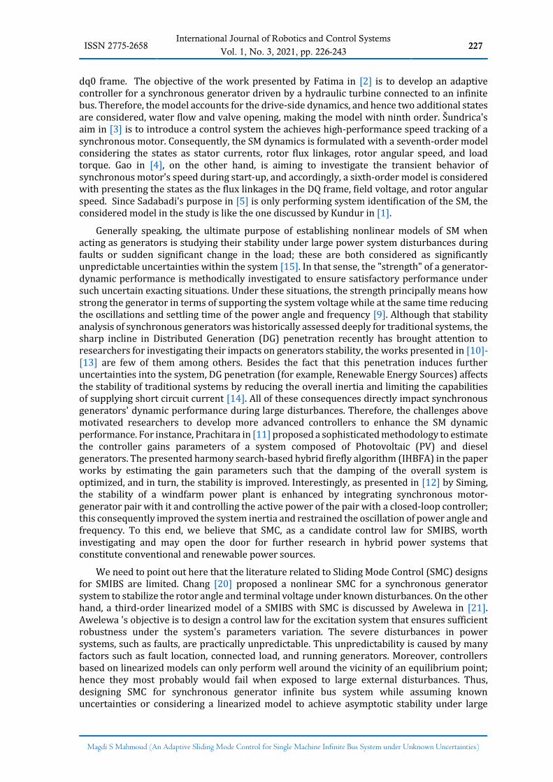
As stated earlier, the model selection is usually based on the objective of the study. This work aims to develop a control law that asymptotically stabilizes the terminal voltage and power angle of an SM connected to an infinite bus using field voltage and mechanical torque as control variables. Hence, the selected model is quite similar to the nonlinear electro-mechanical seventh-order presented by Fodor in [6], with, however, minor modifications derived from [7]. Note that all variables and parameters mentioned henceforth are defined in Table 1 and Table 2, respectively. The overall power system that is under investigation is shown in Fig. 1.


229 Vol. 1, No. 3, 2021, pp. 226-243


Fig. 1. Single Machine Infinite Bus System (SMIBS) schematic

Table 1. SMIBS nonlinear model variables definitions

Variable Type Description

𝑖𝑑 State Projection of line current in d-axis

𝑖𝑞 State Projection of line current in q-axis

𝑖𝐹 State Field winding current

𝜔 State Rotor mechanical angular velocity

𝑣𝑓 Input Field winding voltage

𝑇𝑚𝑒𝑐ℎ Input Mechanical driver torque

𝑣𝑡(𝑥), 𝑣𝑑 , 𝑣𝑞 State, output Machine terminal voltage and projection of line voltages in the dq

frame

𝜗 State, output Electrical power angle in rad

Table 2. SMIBS parameters definitions

Parameter Description Values (pu) [2]

𝑟𝑠 Stator winding resistance 1•10-3

𝑟𝐹 Rotor field winding resistance 7.40•10-4

𝐿𝑑 d-axis stator inductance 1.70

𝐿𝑞 q-axis stator inductance 1.64

𝐿𝐹 Rotor field winding inductance 1.65

𝑀𝐹 Stator-to-rotor mutual inductance 1.89

𝑅𝑒 Transmission line and/or transformer equivalent resistance* 0.2

𝐿𝑒 Transmission line and/or transformer equivalent inductance* 1.64

𝑉∞ Infinite bus phase rms voltage 1.00

𝜔𝑟 Angular velocity of stator magnetic field 1.00

𝜃 Infinite bus angle 0

𝐻 Inertia constant 3.195

𝐷 Damping constant 2.004

*Representing the equivalent impendence from the generator terminal to the infinite bus

Considering 𝑣𝑓 and 𝑇𝑚𝑒𝑐ℎ as the model inputs, the overall state-space model is described as

follows:

�̇� = 𝐹(𝑥) + 𝑩𝑢, 𝑦 = [𝑣𝑡(𝑥) 𝑥4]𝑇 (1)

Where

𝑥 = [𝑖𝑑 𝑖𝑞 𝑖𝐹 𝜗 𝜔]T = [𝑥1 𝑥2 𝑥3 𝑥4 𝑥5]T;

𝐹(𝑥) =

[

𝐴11𝑥1 + 𝐴12𝑥3 + 𝐴13𝑥2𝑥5 + 𝐴14 sin(𝑥4 − 𝜃)

𝐴21𝑥1𝑥5 + 𝐴22𝑥3𝑥5 + 𝐴23𝑥2 + 𝐴24 cos(𝑥4 − 𝜃)

𝐴31𝑥1 + 𝐴32𝑥3 + 𝐴33𝑥2𝑥5 + 𝐴34 sin(𝑥4 − 𝜃)

(𝑥5 − 1)𝜔𝑟

𝐴51𝑥1𝑥2 + 𝐴52𝑥2𝑥3 + 𝐴53𝑥5 ]

;


ISSN 2775-2658 Vol. 1, No. 3, 2021, pp. 226-243


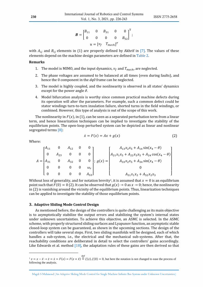
𝑩 = [𝐵11 0 𝐵31 0 0

0 0 0 0 𝐵52

]

T

;

𝑢 = [𝑣𝑓 𝑇𝑚𝑒𝑐ℎ]𝑇

with 𝐴𝑖𝑗 and 𝐵𝑖𝑗 elements in (1) are properly defined by Akhrif in [7]. The values of these

elements depend on the machine design parameters are defined in Table 2.

Remarks

1. The model is MIMO, and the input dynamics, 𝑣𝑓 and 𝑇𝑚𝑒𝑐ℎ, are neglected.

2. The phase voltages are assumed to be balanced at all times (even during faults), and hence the 0 component in the dq0 frame can be neglected.

3. The model is highly coupled, and the nonlinearity is observed in all states' dynamics except for the power angle 𝜗.

4. Model bifurcation analysis is worthy since common practical machine defects during its operation will alter the parameters. For example, such a common defect could be stator windings turn-to-turn insulation failure, shorted turns in the field windings, or combined. However, this type of analysis is out of the scope of this work.

The nonlinearity in 𝐹(𝑥), in (1), can be seen as a separated perturbation term from a linear term, and hence linearization techniques can be implied to investigate the stability of the equilibrium points. The open-loop perturbed system can be depicted as linear and nonlinear segregated terms [8]:

�̇� = 𝐹(𝑥) = 𝐴𝑥 + 𝑔(𝑥) (2)

Where:

𝐴 =

[ 𝐴11 0 𝐴12 0 0

0 𝐴23 0 0 0

𝐴31 0 𝐴32 0 0

0 0 0 0 𝜔𝑟

0 0 0 0 𝐴53]

; 𝑔(𝑥) =

[

𝐴13𝑥2𝑥5 + 𝐴14 sin(𝑥4 − 𝜃)

𝐴21𝑥1𝑥5 + 𝐴22𝑥3𝑥5 + 𝐴24 cos(𝑥4 − 𝜃)

𝐴33𝑥2𝑥5 + 𝐴34 sin(𝑥4 − 𝜃)

0

𝐴51𝑥1𝑥2 + 𝐴52𝑥2𝑥3 ]

Without loss of generality, and for notation brevity1, it is assumed that 𝑥 = 0 is an equilibrium point such that 𝐹(0) = 0 (2). It can be observed that 𝑔(𝑥) → 0 as 𝑥 → 0; hence, the nonlinearity in (2) is vanishing around the vicinity of the equilibrium points. Thus, linearization techniques can be applied to investigate the stability of those equilibrium points.

3. Adaptive Sliding Mode Control Design

As mentioned before, the design of the controllers is quite challenging as its main objective is to asymptotically stabilize the output errors and stabilizing the system's internal states under unknown uncertainties. To achieve this objective, an ASMC is selected. In the ASMC scheme, with properly structured sliding surfaces and Lyapunov function, an asymptotic stable closed-loop system can be guaranteed, as shown in the upcoming sections. The design of the controllers will take several steps. First, two sliding manifolds will be designed, each of which handles a sub-system, i.e., the electrical and the mechanical sub-systems. After that, the reachability conditions are deliberated in detail to select the controllers' gains accordingly. Like Edwards et al. method [18], the adaptation rules of these gains are then derived so that

1 𝑧 = 𝑥 − �̅� → �̇� = �̇� = 𝐹(𝑥) = 𝐹(𝑧 + �̅�) =⏞def

𝜉(𝑧), 𝜉(0) = 0, but here the notation is not changed to ease the process of

following the analysis.


231 Vol. 1, No. 3, 2021, pp. 226-243


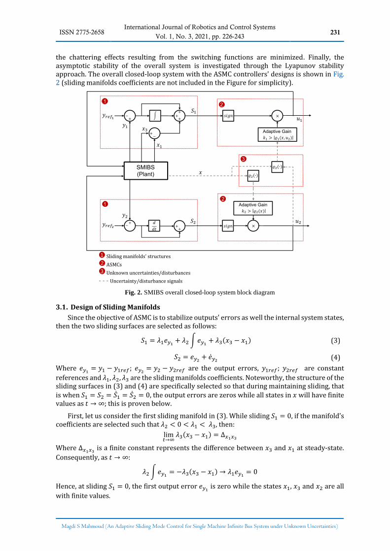
the chattering effects resulting from the switching functions are minimized. Finally, the asymptotic stability of the overall system is investigated through the Lyapunov stability approach. The overall closed-loop system with the ASMC controllers' designs is shown in Fig. 2 (sliding manifolds coefficients are not included in the Figure for simplicity).

Sliding manifolds' structures

ASMCs

Unknown uncertainties/disturbances

- - - Uncertainty/disturbance signals

Fig. 2. SMIBS overall closed-loop system block diagram

Design of Sliding Manifolds

Since the objective of ASMC is to stabilize outputs' errors as well the internal system states, then the two sliding surfaces are selected as follows:

𝑆1 = 𝜆1𝑒𝑦1+ 𝜆2 ∫𝑒𝑦1

+ 𝜆3(𝑥3 − 𝑥1) (3)

𝑆2 = 𝑒𝑦2+ �̇�𝑦2

(4)

Where 𝑒𝑦1= 𝑦1 − 𝑦1𝑟𝑒𝑓; 𝑒𝑦2

= 𝑦2 − 𝑦2𝑟𝑒𝑓 are the output errors, 𝑦1𝑟𝑒𝑓; 𝑦2𝑟𝑒𝑓 are constant

references and 𝜆1, 𝜆2, 𝜆3 are the sliding manifolds coefficients. Noteworthy, the structure of the sliding surfaces in (3) and (4) are specifically selected so that during maintaining sliding, that is when 𝑆1 = 𝑆2 = �̇�1 = �̇�2 = 0, the output errors are zeros while all states in 𝑥 will have finite values as 𝑡 → ∞; this is proven below.

First, let us consider the first sliding manifold in (3). While sliding 𝑆1 = 0, if the manifold's coefficients are selected such that 𝜆2 < 0 < 𝜆1 < 𝜆3, then:

lim𝑡→∞

𝜆3(𝑥3 − 𝑥1) = ∆𝑥1𝑥3

Where ∆𝑥1𝑥3 is a finite constant represents the difference between 𝑥3 and 𝑥1 at steady-state.

Consequently, as 𝑡 → ∞:

𝜆2 ∫𝑒𝑦1= −𝜆3(𝑥3 − 𝑥1) → 𝜆1𝑒𝑦1

= 0

Hence, at sliding 𝑆1 = 0, the first output error 𝑒𝑦1 is zero while the states 𝑥1, 𝑥3 and 𝑥2 are all

with finite values.

1

2

3


ISSN 2775-2658 Vol. 1, No. 3, 2021, pp. 226-243


For the second sliding surface in (4), during sliding 𝑆2 = 0, the two terms must equal to zero:

𝑒𝑦2= �̇�𝑦2

= 0

Since 𝑦2 = 𝑥4, this implies:

𝑒𝑦2= 𝑦2 − 𝑦2𝑟𝑒𝑓 = 𝑥4 − 𝑦2𝑟𝑒𝑓 = 0 → 𝑥4 = 𝑦2 = 𝑦2𝑟𝑒𝑓 (5)

From the dynamics of 𝑥4 in F(x) in (1) and the fact that of �̇�𝑦2= 0 when 𝑆2 = 0:

�̇�𝑦2= �̇�4 = (𝑥5 − 1)𝜔𝑟 = 0

As 𝑡 → ∞:

�̇�4 = (𝑥5 − 1)𝜔𝑟 = 0 → 𝑥5 = 1

Hence the second output error 𝑒𝑦2 is zero while 𝑥4 and 𝑥5 both have finite values as 𝑡 → ∞

when 𝑆2 = 0.

Reachability Conditions

To guarantee reachability of errors and states trajectories into the surfaces 𝑆1 = 𝑆2 = 0, both conditions 𝑆1�̇�1 < 0 and 𝑆2�̇�2 < 0 shall be achieved. The achievability of reaching these manifolds is proven separately in the following subsections.

1) Reachability Condition of First Sliding Manifold

Let us first consider 𝑆1 and its reachability condition 𝑆1�̇�1 < 0. From (3), the dynamics of the first sliding surface is given by:

�̇�1 = 𝜆1�̇�𝑦1+ 𝜆2𝑒𝑦1

+ 𝜆3(�̇�3 − �̇�1) = 𝜆1�̇�1 + 𝜆2(𝑦1 − 𝑦1𝑟𝑒𝑓) + 𝜆3(�̇�3 − �̇�1) (6)

The first output is a function of the states such that 𝑦1 = 𝑣𝑡(𝑥), then:

�̇�1 = 𝜆1�̇�1 + 𝜆2[𝑣𝑡(𝑥) − 𝑦1𝑟𝑒𝑓] + 𝜆3(�̇�3 − �̇�1) (7)

Also, the first input 𝑢1 = 𝑣𝑓 appears in �̇�1:

�̇�1 = �̇�𝑡(𝑥) =1

2(𝑣𝑑

2 + 𝑣𝑞2)

−12 ∙ (2𝑣𝑑�̇�𝑑 + 2𝑣𝑞�̇�𝑞) (8)

𝑢1 specifically appears in �̇�𝑑 and �̇�𝑞:

�̇�𝑑 = (𝑅𝑒 + 𝐿𝑒𝐴11)�̇�1 + 𝐿𝑒𝐴12�̇�3 + (𝐿𝑒𝐴13 − 𝐿𝑒)(�̇�2𝑥5 + 𝑥2�̇�5)

+ (𝑉∞ + 𝐿𝑒𝐴14)�̇�4 cos(𝑥4 − 𝛼)

�̇�𝑞 = (𝑅𝑒 + 𝐿𝑒𝐴33)�̇�2 + (𝐿𝑒𝐴21 − 𝐿𝑒)(�̇�1𝑥5 + 𝑥1�̇�5) + 𝐿𝑒𝐴22(�̇�3𝑥5 + 𝑥3�̇�5)

− (𝑉∞ + 𝐿𝑒𝐴24)�̇�4 sin(𝑥4 − 𝛼)

(9)

Where it can be observed from (1) that 𝑢1 appears in �̇�1 and �̇�3. Noteworthy, the second input 𝑢2 also appears in �̇�1through �̇�5 by tracking (1), (8), and (9). Hence, from (1), (7), (8), and (9), it can be concluded that the dynamics of the first sliding surface is a function of the states and both inputs and can be described in the following general form:

�̇�1 = ℎ1(𝑥, 𝑢2) + 𝑧1(𝑥)𝑢1 (10)

Consider the following controller:

𝑢1 = −[𝑘1(𝑡) + 𝜂1]𝑠𝑖𝑔𝑛(𝑆1) (11)

Where 𝑘1(𝑡) is the controller gain and 𝜂1 is a constant. The dynamics of the sliding surface in (10) now can be expanded as:

�̇�1 = ℎ1(𝑥, 𝑢2) − 𝑧1(𝑥)[𝑘1(𝑡) + 𝜂1]𝑠𝑖𝑔𝑛(𝑆1) (12)

Define a bounded uncertainty such that:


233 Vol. 1, No. 3, 2021, pp. 226-243


𝜚1(𝑥, 𝑢2) =ℎ1(𝑥, 𝑢2)

𝑧1(𝑥)< 𝜚10 (13)

It is clear from (12) and (13) that if the controller gain is selected such that 𝑘1(𝑡) >|𝜚1(𝑥, 𝑢2)|, then the reachability condition of the first sliding manifold 𝑆1�̇�1 < 0 is achieved. Note that the gain 𝑘1(𝑡) is a function of time since it is adaptive, and the design of it is discussed in sections 3-3. Also, from (13), the signal of the second controller is considered an uncertainty that the first controller shall absorb. Therefore, an essential condition to secure the boundness of 𝜚1 is bounding the second controller such that 𝑢2 < 𝑢20 where 𝑢20 is a predefined constant. Next, the reachability condition of the second manifold is discussed.

2) Reachability Condition of Second Sliding Manifold

As discussed earlier, to guarantee the reachability to the surface 𝑆2 = 0, then the condition 𝑆2�̇�2 < 0 shall be satisfied. The dynamics of the second sliding surface defined in (4) is given by:

�̇�2 = �̇�𝑦2+ �̈�𝑦2

(14)

Since 𝑒𝑦2 = 𝑥4 − 𝑦2𝑟𝑒𝑓 and the second derivative of 𝑥4 is a function of �̇�5, then:

�̇�2 = �̇�4 + �̈�4 = �̇�4 + 𝜔𝑟�̇�5 (15)

Where the second controller 𝑢2 appears in �̇�5. Consequently, the derivative of the second sliding surface can be written in the following general structure:

�̇�2 = ℎ2(𝑥) + 𝑧2(𝑥)𝑢2 (16)

Consider the controller:

𝑢2 = −[𝑘2(𝑡) + 𝜂2]𝑠𝑖𝑔𝑛(𝑆2) (17)

Where 𝑘2(𝑡) is the controller gain and 𝜂2 is a constant. The dynamics of the sliding surface in (16) can be then expanded as:

�̇�2 = ℎ2(𝑥) − 𝑧2(𝑥)[𝑘2(𝑡) + 𝜂2]𝑠𝑖𝑔𝑛(𝑆2) (18)

Define a bounded uncertainty such that:

𝜚2(𝑥) =ℎ2(𝑥)

𝑧2(𝑥)< 𝜚20 (19)

It is clear from (18) and (19) that if the controller gain is selected such that 𝑘2(𝑡) > |𝜚2(𝑥)|, then the reachability condition of the second sliding manifold 𝑆2�̇�2 < 0 is achieved. So far, we

have proved that the reachability conditions of 𝑆1�̇�1 < 0 and 𝑆2�̇�2 < 0 are only guaranteed if 𝑘1(𝑡) > |𝜚1(𝑥, 𝑢2)| and 𝑘2(𝑡) > |𝜚2(𝑥)|. Therefore, it is required now to design these controllers' gains, with adaptation rules, to achieve these conditions while mitigating chattering effects as much as possible.

Derivation of Controllers Gains Adaptation Rule

It is well-known that one of the main drawbacks of SMC is the associated "chattering" effects resulted from the inherent switching function within the controller [16]. Although that chattering affects the power angle and machine rotor speed (𝑥5) may be acceptable, the appearance of this phenomenon in the machine terminal voltage (𝑦1) and the currents (𝑥1, 𝑥2 and 𝑥3) will cause a catastrophic impact on the power quality due to the associated harmonics with the chattering. One of the proven solutions for chattering is the adaptive scheme of SMC, and they are, for example, discussed by Utkin in [17] and by Edwards in [18]. The ASMC incorporates an adaptive controller gain such that it is as small as possible to mitigate chattering while simultaneously guarantees a sliding motion that offsets a bounded uncertainty. Therefore, the ASMC scheme is implemented in this work and discussed in the following subsections.


ISSN 2775-2658 Vol. 1, No. 3, 2021, pp. 226-243


The development of the adaptation rule will compose of several steps. First, an estimated equivalent controller instead of the actual will be used to develop the rule. More importantly, the controllers' gains' adaptation rule will have two nested adaptation layers as described in [18]. The first layer of adaptation is designed so that the gain 𝑘 varies with the magnitude of the sliding surface dynamics to offset the bounded uncertainty. On the other hand, the second layer will take care of the gain rate of change to guarantee that the dynamics of 𝑘 follow the

bounded uncertainty rate of change such that �̇� > �̇�(𝑥).

Noteworthy, since the derivation of both controllers' gains 𝑘1(𝑡) and 𝑘2(𝑡) is similar, the subscript i = 1, 2 to represent the first and second controllers, respectively, is used henceforth for notation brevity. Also, |𝜚1(𝑥, 𝑢2)| will be described as |𝜚1(𝑥)| for brevity.

Let us first define the equivalent controller that will be used to derive the gains adaptation rule. To maintain sliding on the surface 𝑆𝑖 = �̇�𝑖 = 0, one shall have an equivalent controller that exactly cancels the bounded disturbance such that:

|𝑢𝑒𝑞𝑖| = |𝜚(𝑥)𝑖| (20)

According to Utkin in [19], this equivalent controller can be estimated as �̅�𝑒𝑞𝑖 in real-time by a

low-pass filter as follows:

�̇̅�𝑒𝑞𝑖=

1

𝜏[−[𝑘𝑖(𝑡) + 𝜂𝑖]𝑠𝑖𝑔𝑛(𝑆𝑖) − �̅�𝑒𝑞𝑖

] (21)

Where 𝜏 is a positive constant that ensures the equivalent controller estimate error |𝑢𝑒𝑞𝑖

− �̅�𝑒𝑞𝑖| is small. From (20) and the requirement of 𝑘𝑖(𝑡) > |𝜚𝑖(𝑥)|, it is clear that the

condition 𝑘𝑖(𝑡) > |𝑢𝑒𝑞𝑖| shall be satisfied to enforce sliding. However, since an estimate of the

equivalent control is used instead of the actual, a safety margin should be introduced as follows:

𝑘𝑖(𝑡) >1

𝛼𝑖|�̅�𝑒𝑞𝑖

| + 𝜖𝑖 (22)

Where 0 < 𝛼𝑖 < 1 and 𝜖𝑖 > 0 are constants, and their selection will be discussed in sections 3-

4. These constants are implemented to ensure that the controller estimates satisfy:

1


| +𝜖𝑖

2⁄ > |𝑢𝑒𝑞𝑖| (23)

And by defining an error term such that [18]:

𝛿𝑖(𝑡) = 𝑘𝑖(𝑡) −1


| − 𝜖𝑖 (24)

If 𝛿𝑖(𝑡) → 0, then:

𝑘𝑖(𝑡) =1


| + 𝜖𝑖 (25)

From (23) and (25), it can be seen that:

𝑘𝑖(𝑡) > |�̅�𝑒𝑞𝑖| = |𝜚𝑖(𝑥)| (26)

Hence, if it is guaranteed that 𝛿𝑖(𝑡) → 0 as 𝑡 → ∞, such that 𝑘𝑖(𝑡) + 𝜂𝑖 > |𝜚𝑖(𝑥)|, then forcing sliding motion is achieved.

Now, the two nested adaptation layers of 𝑘𝑖(𝑡) are derived as follows. First, we will define the adaptation of 𝑘𝑖(𝑡), that is the first adaptive layer, as [18]:

�̇�𝑖(𝑡) = −𝜌𝑖(𝑡) ∙ 𝑠𝑖𝑔𝑛[𝛿𝑖(𝑡)] (27)

Where 𝜌𝑖(𝑡) is a function of time and represents the upper bound of the uncertainty dynamics |𝜚�̇�(𝑥)| < 𝜚𝑖𝑖 and it has the following form:


235 Vol. 1, No. 3, 2021, pp. 226-243


𝜌𝑖(𝑡) = 𝑟𝑖0 + 𝑟𝑖(𝑡) (28)

Where 𝑟𝑖0 is a design scalar (selection of it is discussed in section 3.4) and 𝑟𝑖(𝑡) is the second adaptation rule in our scheme. Assuming the uncertainty bounds are unknown (both 𝜚𝑖0 and 𝜚𝑖𝑖 are unknown), the adaptation rule of 𝑟𝑖(𝑡) given by [18] is:

�̇�𝑖(𝑡) = {𝛾𝑖|𝛿𝑖(𝑡)|; |𝛿𝑖(𝑡)| > 𝛿𝑖0

0; 𝑜𝑡ℎ𝑒𝑟𝑤𝑖𝑠𝑒 (29)

Where 𝛿𝑖0 > 0 and 𝛾𝑖 > 0 are both design scalars, and their selection will be discussed in section 3.4. To allow 𝑟𝑖(𝑡) tracks the rate of change of the uncertainty, we define an error function as:

𝑒𝑖(𝑡) =𝑞𝑖𝜚𝑖𝑖

𝛼𝑖− 𝑟𝑖(𝑡) (30)

Where 𝑞𝑖 > 1 is a safety factor to ensure �̇̅�𝑒𝑞𝑖< 𝑞𝑖𝜚𝑖𝑖.

Lyapunov Stability Analysis

The stability analysis is crucial to investigate the asymptotic stability of the overall closed-loop system along with the output errors. As discussed earlier, reaching the sliding manifolds and maintaining sliding guarantee asymptotically stable outputs errors and internal states of the system. However, reaching the surface can only be guaranteed if 𝑘1(𝑡) > |𝜚1(𝑥, 𝑢2)| and 𝑘2(𝑡) > |𝜚2(𝑥)|. It was also shown that these conditions are met if the error functions defined in (24) and (30) are approaching zero as 𝑡 → ∞. Therefore, a reasonable candidate for a Lyapunov function is a quadratic one in terms of the sliding manifolds and errors defined in (3)-(4) and (24)-(30), respectively:

V =1

2𝛿1

2 +1

𝛾12𝑒1

2 +1

2𝛿2

2 +1

𝛾22𝑒2

2 +1

2𝑆1

2 +1

2𝑆2

2 (31)

The derivative of this Lyapunov is:

V̇ = 𝛿1�̇�1 +1

𝛾1𝑒1�̇�1 + 𝛿2�̇�2 +

1

𝛾2𝑒2�̇�2 + 𝑆1�̇�1 + 𝑆2�̇�2 (32)

And from (31), the derivative of 𝛿𝑖 for i = 1, 2 is:

�̇�𝑖 = �̇�𝑖 −1

𝛼𝑖|�̇̅�𝑒𝑞𝑖

| = −(𝑟𝑖0 +𝑞𝑖𝜚𝑖𝑖

𝛼𝑖− 𝑒𝑖) 𝑠𝑖𝑔𝑛(𝛿𝑖) −

𝑞𝑖𝜚𝑖𝑖

𝛼𝑖 (33)

While the derivative of e from (30) is:

�̇�𝑖 = −�̇�𝑖 (34)

Hence:

𝛿𝑖�̇�𝑖 ≤ −𝑟𝑖0|𝛿𝑖| + (𝑒𝑖 −𝑞𝑖𝜚𝑖𝑖

𝛼𝑖) |𝛿𝑖| + |𝛿𝑖|

𝑞𝑖𝜚𝑖𝑖

𝛼𝑖= −𝑟𝑖0|𝛿𝑖| + 𝑒𝑖|𝛿𝑖| (35)

It also can be seen that 𝑒𝑖 ≤𝑞𝑖𝜚𝑖𝑖

𝛼𝑖 since 𝑟𝑖 ≥ 0. Let us now examine the derivative of the

Lyapunov function at both conditions of the adaption of 𝑟𝑖 defined in (29). If |𝛿𝑖| > 𝛿𝑖0, then substituting (34) and (35) into (32) yields to:

V̇ = −𝑟10|𝛿1| + 𝑒1|𝛿1| −1

𝛾1𝑒1�̇�1−𝑟20|𝛿2| + 𝑒2|𝛿2| −

1

𝛾2𝑒2�̇�2 + 𝑆1�̇�1 + 𝑆2�̇�2 (36)

Substituting (36) into (43) yields:

V̇ = −𝑟10|𝛿1| + 𝑒1|𝛿1| − 𝑒1|𝛿1| −𝑟20|𝛿2| + 𝑒2|𝛿2| − 𝑒2|𝛿2| + 𝑆1�̇�1 + 𝑆2�̇�2

= −𝑟10|𝛿1|−𝑟20|𝛿2| + 𝑆1�̇�1 + 𝑆2�̇�2 (37)


ISSN 2775-2658 Vol. 1, No. 3, 2021, pp. 226-243


If |𝛿| < 𝛿0, then 𝑟�̇� = 0 and 𝑒𝑖 < 0 since 𝑟𝑖 ≥𝑞𝑖𝜚𝑖𝑖

𝛼𝑖; hence from (36) also:

V̇ = −𝑟10|𝛿1| + 𝑒1|𝛿1| − 𝑟20|𝛿2| + 𝑒2|𝛿2| + 𝑆1�̇�1 + 𝑆2�̇�2 (38)

Since the error terms in the Lyapunov derivative in (37) and (38) at both values of 𝑟�̇� are negative, then 𝛿𝑖 , 𝑒𝑖 → 0 as 𝑡 → ∞. Consequently, the condition 𝑘𝑖(𝑡) > |𝜚𝑖(𝑥)| is achieved, and

as a result, the terms 𝑆1�̇�1 and 𝑆2�̇�2 in (37) and (38) are both negative. Therefore, the derivative of this Lyapunov is semi-negative definite since V̇(0) = 0. However, at 𝛿𝑖 = 𝑒𝑖 = 𝑆𝑖 = 0, the sliding on the manifolds is attainable and maintained, resulting in stable output errors and internal states as discussed in sections 3.1 and 3.3. Since this is the case and V is radially unbounded positive definite, then the output errors and the system's internal states are asymptotically stable under the condition of bounded uncertainties defined by 𝜚𝑖0 and 𝜚𝑖𝑖 .

Remarks

From (37) and (38), the selection of 𝑟𝑖0 constitutes the decaying rate of the gain errors defined in (24) and consequently how fast the states and outputs errors trajectories will start moving toward the sliding manifolds.

The controllers' coefficients 𝜖𝑖, 𝛼𝑖, 𝛿𝑖0 and 𝛾𝑖 shall be selected such that:

1

4𝜖𝑖

2 > 𝛿𝑖02 +

1

𝛾𝑖(𝑞𝑖𝜚𝑖𝑖

𝛼𝑖)2

(39)

to guarantee asymptotic stable gain errors, defined in (24) and (30), and to secure bounded controllers' gains [18].

4. Simulation and discussion

The simulation is carried out on the SMIBS shown in Fig. 1 with two different closed-loop control systems. The first governs our design shown in Fig. 2, while the second is a conventional SMC with constant gains for performance comparison. The main objective of the simulation is to verify the effectiveness of the designed ASMC in terms of chattering mitigation and to assess its capability in achieving asymptotic stable output errors and stabilizing the systems' internal states, such that lim

𝑡→∞𝑒𝑦 = 0 and lim

𝑡→∞𝑥 = 𝑥𝑓 , under the presence of severe disturbance. The

disturbances defined previously by 𝜚1(𝑥, 𝑢2) and 𝜚2(𝑥) will also be "momentarily" perturbed during the simulation by altering the infinite bus voltage, that is, in particular, altering the parameter 𝑉∞. With this, we eventually simulate a short circuit fault on the SM bus that is cleared within finite time. We then assess the system's overall closed-loop performance under such severe conditions and compare it with conventional SMC.

Scenario

The duration of the simulation is 380 tu (this is around a second). A three-phase fault occurs at 150 tu in the power system's bus, at the location indicated in Fig. 1, and the fault is cleared at 190 tu (fault duration is around 40 tu, which is equivalent to 100 msec). As indicated previously, this system fault is simulated by altering the value of 𝑉∞. In this case, its value will be reduced from 1.0 to 0.5 during the fault only; when the fault is cleared, 𝑉∞ returns to its nominal value of 1.0. For the output references 𝑦1𝑟𝑒𝑓 and 𝑦2𝑟𝑒𝑓 , a reasonable selection is 1.0

and 0.15 𝑟𝑎𝑑, respectively. For 𝑦1𝑟𝑒𝑓 , since the SM is connected to an infinite bus with 𝑉∞ =

1.0 nominal, then the SM is expected to operate at the same voltage level during a steady-state condition. On the other hand, 𝑦2𝑟𝑒𝑓 , the power angle of the SM should be positive since the SM

is running on generation mode.

The sliding manifolds and the controller coefficients are selected based on the discussions in sections 3.1 and 3.4, respectively, and their values are depicted in Table 3. Note that 𝛾1, 𝛾2 are both chosen to be sufficiently large, and 𝛼1, 𝛼2 are set at the high side of their allowable range to ensure reducing the right-hand side of inequality (39), and hence the inequality is


237 Vol. 1, No. 3, 2021, pp. 226-243


satisfied. The values of 𝛿10, 𝛿20 are adjusted to be as small as possible while at the same time avoiding any potential computational errors during simulation, as suggested in [18]. For the SMC gains, they are selected to be sufficiently large to offset the unseen disturbances. The parameters' values of the nonlinear SMIBS model, 𝐴𝑖𝑗 and 𝐵𝑖𝑗 , are shown in Table 4. As

indicated previously, these values are functions of the system's components.

Results

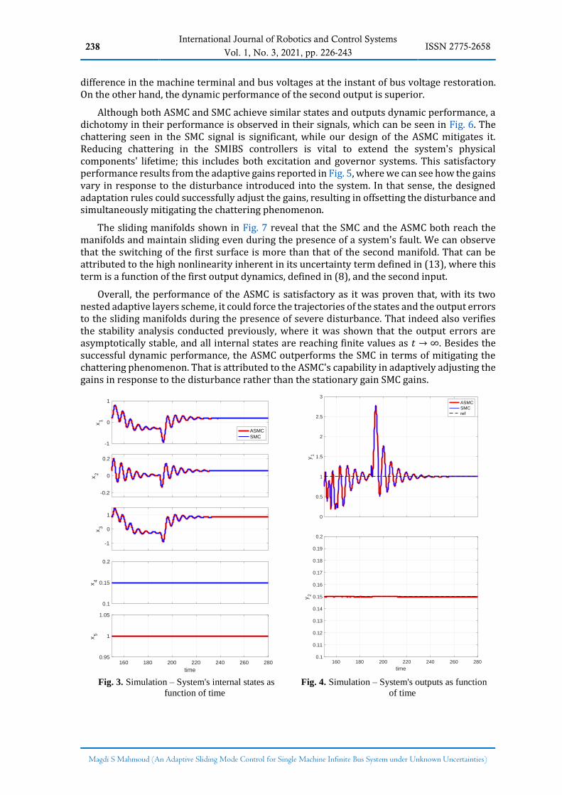
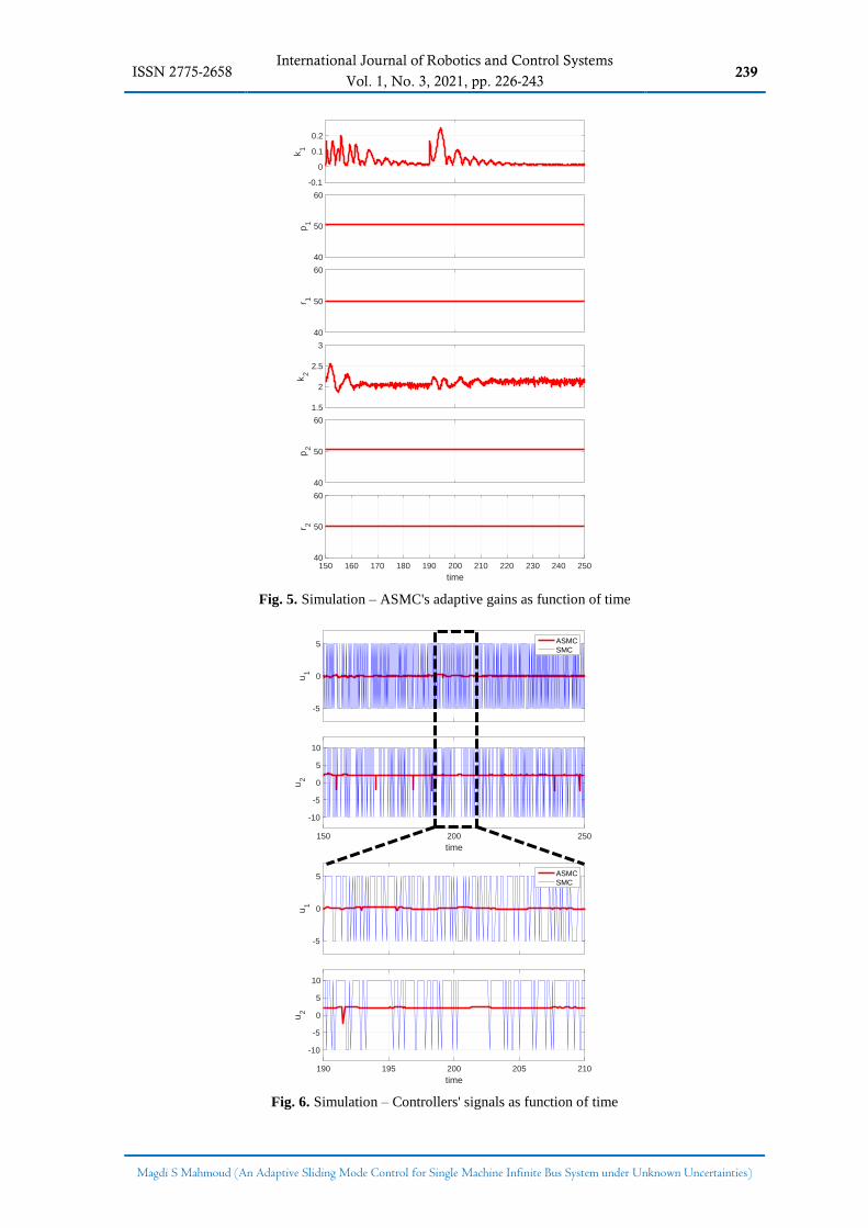
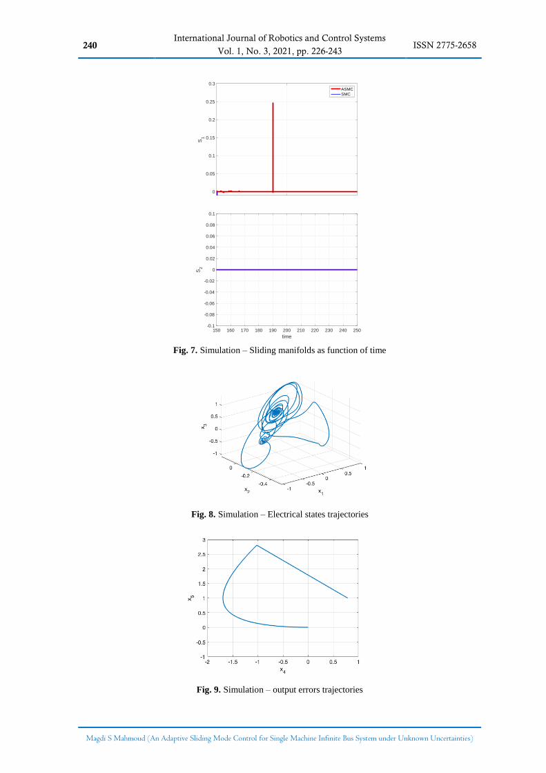
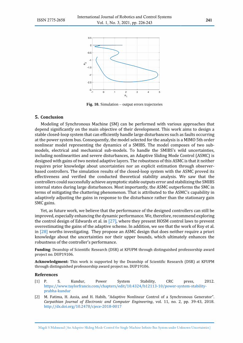
All results of the simulation during and after the fault are represented in plots. The internal states of the system are shown in Fig. 3, while the outputs are shown in Fig. 4. Also, the controllers' signals are shown in Fig. 6; meanwhile, the ASMC gains are reported in Fig. 5. The sliding manifolds are illustrated in Fig. 7. Finally, the trajectories of electrical states 𝑥1, 𝑥2, 𝑥3 are shown in Fig. 8, the trajectories of the mechanical states 𝑥4, 𝑥5 are depicted in Fig. 9, and the output errors are in Fig. 10.

Table 3. Sliding manifolds and controllers' coefficients values

Coefficient Assignee Value

𝜆1 First Sliding Manifold 1.00

𝜆2 First Sliding Manifold -1.00

𝜆3 First Sliding Manifold 10.0

𝜖1, 𝜖2 ASMC 0.01

𝛿10 , 𝛿20 ASMC 0.05

𝑟10, 𝑟20 ASMC 0.5

𝛼1, 𝛼2 ASMC 0.99

𝛾1, 𝛾2 ASMC 400

𝜂1, 𝜂2 ASMC 0.05

𝜏 ASMC 0.01

𝑘1 SMC 5.00

𝑘2 SMC 10.0

Table 4. SMIBS parameters' values

Parameter Value Parameter Value Parameter Value

𝐴11 -0.173 𝐴23 0.06128 𝐴51 0.00939

𝐴12 -0.000734 𝐴24 -0.3049 𝐴52 -0.2958

𝐴13 2.823 𝐴31 -0.1994 𝐴53 -0.3136

𝐴14 -0.8607 𝐴32 -0.001297 𝐵11 0.9919

𝐴21 -1.018 𝐴33 3.253 𝐵31 1.753

𝐴22 0.5762 𝐴34 -0.9919 𝐵52 0.1565

Discussion

The system's internal states and outputs, depicted in Fig. 3 and Fig. 4, respectively, are asymptotically stabilized after the fault clearance with almost similar performance observed with ASMC and SMC. That asymptotic stability is also indicated by the electrical and mechanical states trajectories depicted in Fig. 8 and Fig. 9, respectively. Although the overshooting observed within the electrical states are acceptable, around rated values of 1, the oscillations are rather high. On the other hand, a remarkable performance of the controllers, ASMC and SMC, can be observed in the mechanical states as their dynamic response during the fault was negligible; this is also seen in their trajectories shown in Fig. 9. For the input-output responses depicted in Fig. 4, the controllers could successfully force them to follow the reference signals after clearing the fault at 190 tu, proving the asymptotic stability of the output errors discussed in section 3.4. The errors' trajectories depicted in Fig. 10 also confirm this as they settle at zero. Noteworthy, the dynamic response of the first output experienced large momentarily overshoot and oscillation when the fault was cleared. Although that response may affect the SM's windings insulation, the overshoot (or voltage surge in power system terminology) is expected when the infinite bus voltage is restored to its nominal value. This is attributed to the


ISSN 2775-2658 Vol. 1, No. 3, 2021, pp. 226-243


difference in the machine terminal and bus voltages at the instant of bus voltage restoration. On the other hand, the dynamic performance of the second output is superior.

Although both ASMC and SMC achieve similar states and outputs dynamic performance, a dichotomy in their performance is observed in their signals, which can be seen in Fig. 6. The chattering seen in the SMC signal is significant, while our design of the ASMC mitigates it. Reducing chattering in the SMIBS controllers is vital to extend the system's physical components' lifetime; this includes both excitation and governor systems. This satisfactory performance results from the adaptive gains reported in Fig. 5, where we can see how the gains vary in response to the disturbance introduced into the system. In that sense, the designed adaptation rules could successfully adjust the gains, resulting in offsetting the disturbance and simultaneously mitigating the chattering phenomenon.

The sliding manifolds shown in Fig. 7 reveal that the SMC and the ASMC both reach the manifolds and maintain sliding even during the presence of a system's fault. We can observe that the switching of the first surface is more than that of the second manifold. That can be attributed to the high nonlinearity inherent in its uncertainty term defined in (13), where this term is a function of the first output dynamics, defined in (8), and the second input.

Overall, the performance of the ASMC is satisfactory as it was proven that, with its two nested adaptive layers scheme, it could force the trajectories of the states and the output errors to the sliding manifolds during the presence of severe disturbance. That indeed also verifies the stability analysis conducted previously, where it was shown that the output errors are asymptotically stable, and all internal states are reaching finite values as 𝑡 → ∞. Besides the successful dynamic performance, the ASMC outperforms the SMC in terms of mitigating the chattering phenomenon. That is attributed to the ASMC's capability in adaptively adjusting the gains in response to the disturbance rather than the stationary gain SMC gains.

Fig. 3. Simulation – System's internal states as

function of time

Fig. 4. Simulation – System's outputs as function

of time

-1

0

1

x1

ASMC

SMC

-0.2

0

0.2

x2

-1

0

1

x3

0.1

0.15

0.2

x4

160 180 200 220 240 260 280

time

0.95

1

1.05

x5

0

0.5

1

1.5

2

2.5

3

y1

ASMC

SMC

ref

160 180 200 220 240 260 280

time

0.1

0.11

0.12

0.13

0.14

0.15

0.16

0.17

0.18

0.19

0.2

y2


239 Vol. 1, No. 3, 2021, pp. 226-243


Fig. 5. Simulation – ASMC's adaptive gains as function of time

Fig. 6. Simulation – Controllers' signals as function of time

-0.1

0

0.1

0.2

k1

40

50

60

p1

40

50

60

r 1

1.5

2

2.5

3

k2

40

50

60

p2

150 160 170 180 190 200 210 220 230 240 250

time

40

50

60

r 2

-5

0

5

u1

ASMC

SMC

150 200 250

time

-10

-5

0

5

10

u2

-5

0

5

u1

ASMC

SMC

190 195 200 205 210

time

-10

-5

0

5

10

u2


ISSN 2775-2658 Vol. 1, No. 3, 2021, pp. 226-243


Fig. 7. Simulation – Sliding manifolds as function of time

Fig. 8. Simulation – Electrical states trajectories

Fig. 9. Simulation – output errors trajectories

0

0.05

0.1

0.15

0.2

0.25

0.3

S1

ASMC

SMC

150 160 170 180 190 200 210 220 230 240 250

time

-0.1

-0.08

-0.06

-0.04

-0.02

0

0.02

0.04

0.06

0.08

0.1

S2


241 Vol. 1, No. 3, 2021, pp. 226-243


Fig. 10. Simulation – output errors trajectories

5. Conclusion

Modeling of Synchronous Machine (SM) can be performed with various approaches that depend significantly on the main objective of their development. This work aims to design a stable closed-loop system that can efficiently handle large disturbances such as faults occurring at the power system bus. Consequently, the model selected for the analysis is a MIMO 5th order nonlinear model representing the dynamics of a SMIBS. The model composes of two sub-models, electrical and mechanical sub-models. To handle the SMIBS's wild uncertainties, including nonlinearities and severe disturbances, an Adaptive Sliding Mode Control (ASMC) is designed with gains of two nested adaptive layers. The robustness of this ASMC is that it neither requires prior knowledge about uncertainties nor an explicit estimation through observer-based controllers. The simulation results of the closed-loop system with the ASMC proved its effectiveness and verified the conducted theoretical stability analysis. We saw that the controllers could successfully achieve asymptotic stable outputs error and stabilizing the SMIBS internal states during large disturbances. Most importantly, the ASMC outperforms the SMC in terms of mitigating the chattering phenomenon. That is attributed to the ASMC's capability in adaptively adjusting the gains in response to the disturbance rather than the stationary gain SMC gains.

Yet, as future work, we believe that the performance of the designed controllers can still be improved, especially enhancing the dynamic performance. We, therefore, recommend exploring the control design of Edwards et al. in [27], where they present HOSM control laws to prevent overestimating the gains of the adaptive scheme. In addition, we see that the work of Roy et al. in [28] worths investigating. They propose an ASMC design that does neither require a priori knowledge about the uncertainties nor their upper bounds, which ultimately enhances the robustness of the controller's performance.

Funding: Deanship of Scientific Research (DSR) at KFUPM through distinguished professorship award project no. DUP19106.

Acknowledgment: This work is supported by the Deanship of Scientific Research (DSR) at KFUPM through distinguished professorship award project no. DUP19106.

References

[1] P. S. Kundur, Power System Stability, CRC press, 2012. https://www.taylorfrancis.com/chapters/edit/10.4324/b12113-10/power-system-stability-prabha-kundur

[2] M. Fatima, H. Assia, and H. Habib, “Adaptive Nonlinear Control of a Synchronous Generator”. Carpathian Journal of Electronic and Computer Engineering, vol. 11, no. 2, pp. 39-43, 2018. http://dx.doi.org/10.2478/cjece-2018-0017

https://www.taylorfrancis.com/chapters/edit/10.4324/b12113-10/power-system-stability-prabha-kundur

https://www.taylorfrancis.com/chapters/edit/10.4324/b12113-10/power-system-stability-prabha-kundur

http://dx.doi.org/10.2478/cjece-2018-0017


ISSN 2775-2658 Vol. 1, No. 3, 2021, pp. 226-243


[3] M. Šundrica, “Synchronous Machine Nonlinear Control System Based on Feedback Linearization and Deterministic Observers,” In Control Theory in Engineering, p. 145, IntechOpen, 2019. https://dx.doi.org/10.5772/intechopen.89420

[4] W. Gao, A. P. S. Meliopoulos, E. V. Solodovnik, and R. Dougal, “A nonlinear model for studying synchronous machine dynamic behavior in phase coordinates,” In 2005 IEEE International Conference on Industrial Technology, pp. 1092-1097, IEEE, 2005. https://doi.org/10.1109/ICIT.2005.1600798

[5] M. S. Sadabadi, M. Karrari, and O. P. Malik, “Identification of Synchronous Generator Using Nonlinear Feedback Model,” IFAC Proceedings Volumes, vol. 41, no. 2, pp. 10371-10376, 2008. https://doi.org/10.3182/20080706-5-KR-1001.01757

[6] A. Fodor, Model Analysis, Parameter Estimation and Control of a Synchronous Generator, Doctoral Dissertation, 2015. http://real-phd.mtak.hu/588/1/Fodor_Attila_dissertation.pdf

[7] O. Akhrif, F. Okou, L. A. Dessaint, and R. Champagne, “Multi-input multi-output feedback linearization of a synchronous generator,” In Proceedings of 1996 Canadian Conference on Electrical and Computer Engineering, Vol. 2, pp. 586-590 1996. IEEE. https://doi.org/10.1109/CCECE.1996.548221

[8] H. Khalil, Nonlinear systems, 2nd ed, Upper Saddle River, NJ: Prentice Hall, pp. 203-204, 2002.

[9] S. Wei, Y. Zhou, and Y. Huang, “Synchronous motor-generator pair to enhance small signal and transient stability of power system with high penetration of renewable energy,” IEEE Access, vol. 5, pp. 11505-11512, 2017. https://doi.org/10.1109/ACCESS.2017.2716103

[10] J. Chen, and T. O'Donnell, “Parameter constraints for virtual synchronous generator considering stability,” IEEE Transactions on Power Systems, vol. 34, no. 3, pp. 2479-2481, 2019. https://doi.org/10.1109/TPWRS.2019.2896853

[11] P. Satapathy, S. Dhar, and P. K. Dash, “Stability improvement of PV-BESS diesel generator-based microgrid with a new modified harmony search-based hybrid firefly algorithm,” IET Renewable Power Generation, vol. 11, no. 5, pp. 566-577, 2017. http://dx.doi.org/10.1049/iet-rpg.2016.0116

[12] S. Wei, Y. Zhou, and Y. Huang, 2017. “Synchronous motor-generator pair to enhance small signal and transient stability of power system with high penetration of renewable energy,” IEEE Access, vol. 5, pp.11505-11512. https://doi.org/10.1109/ACCESS.2017.2716103

[13] X. Haizhen, Z. Xing, L. Fang, M. Fubin, S. Rongliang, and N. Hua, 2015, November. “An improved virtual synchronous generator algorithm for system stability enhancement,” In 2015 IEEE 2nd International Future Energy Electronics Conference (IFEEC), pp. 1-6, IEEE, 2015. https://doi.org/10.1109/IFEEC.2015.7361571

[14] N. A. Masood, R. Yan, T. K. Saha, and S. Bartlett, ‘‘Post-retirement utilisation of synchronous generators to enhance security performances in a wind dominated power system,’’ IET Gener. Transm. Distrib., vol. 10, no. 13, pp. 3314–3321, Oct. 2016. http://dx.doi.org/10.1049/iet-gtd.2016.0267

[15] "IEEE Guide for Synchronous Generator Modeling Practices and Parameter Verification with Applications in Power System Stability Analyses," in IEEE Std 1110-2019 (Revision of IEEE Std 1110-2002), vol., no., pp.1-92, 2 March 2020. https://doi.org/10.1109/IEEESTD.2020.9020274

[16] A. Levant, “Higher-order sliding modes, differentiation and output-feedback control,” International journal of Control, vol. 76, no. 9-10, pp. 924-941, 2003. http://dx.doi.org/10.1080/0020717031000099029

[17] V. I. Utkin and A. S. Poznyak. “Adaptive sliding mode control with application to super-twist algorithm: Equivalent control method,” Automatica, vol. 49, no. 1, pp.39-47, 2013. http://dx.doi.org/10.1016/j.automatica.2012.09.008

[18] C. Edwards, and Y. B. Shtessel, “Adaptive continuous higher order sliding mode control,” Automatica, 65, pp. 183-190. https://doi.org/10.1016/j.automatica.2015.11.038

[19] V. I. Utkin, Sliding modes in control and optimization, Springer Science & Business Media, 2013.

[20] Y. Chang and C. C. Wen, “Sliding mode control for the synchronous generator,” International Scholarly Research Notices, 2014. http://dx.doi.org/10.1155/2014/256504

[21] A. A. Awelewa, I. A. Samuel, J. Katende, and A. F. Agbetuyi, “Synchronous Generator Excitation Chatter-Free Sliding Mode Controller,” Asian Transactions on Engineering, vol. 2, no, 5, p. 57, 2012. http://eprints.covenantuniversity.edu.ng/id/eprint/3134

https://dx.doi.org/10.5772/intechopen.89420

https://doi.org/10.1109/ICIT.2005.1600798

https://doi.org/10.3182/20080706-5-KR-1001.01757

http://real-phd.mtak.hu/588/1/Fodor_Attila_dissertation.pdf

https://doi.org/10.1109/CCECE.1996.548221

https://doi.org/10.1109/ACCESS.2017.2716103

https://doi.org/10.1109/TPWRS.2019.2896853

http://dx.doi.org/10.1049/iet-rpg.2016.0116

https://doi.org/10.1109/ACCESS.2017.2716103

https://doi.org/10.1109/IFEEC.2015.7361571

http://dx.doi.org/10.1049/iet-gtd.2016.0267

http://dx.doi.org/10.1049/iet-gtd.2016.0267

https://doi.org/10.1109/IEEESTD.2020.9020274

http://dx.doi.org/10.1080/0020717031000099029

http://dx.doi.org/10.1016/j.automatica.2012.09.008

https://doi.org/10.1016/j.automatica.2015.11.038

http://dx.doi.org/10.1155/2014/256504

http://eprints.covenantuniversity.edu.ng/id/eprint/3134


243 Vol. 1, No. 3, 2021, pp. 226-243


[22] C. Edwards and S. K. Spurgeon, “On the development of discontinuous observers,” International Journal of control, vol. 59, no. 5, pp. 1211-1229, 1994. https://doi.org/10.1080/00207179408923128

[23] A. Chalanga, S. Kamal, L. M. Fridman, B. Bandyopadhyay, and J. A. Moreno, “Implementation of super-twisting control: Super-twisting and higher order sliding-mode observer-based approaches,” IEEE Transactions on Industrial Electronics, vol. 63 no. 6, pp. 3677-3685, 2016. https://doi.org/10.1109/TIE.2016.2523913

[24] Y. Shtessel, L. Fridman, and F. Plestan, “Adaptive sliding mode control and observation,” International Journal of Control, vol. 89, no. 9, pp. 1743-1746, 2016. https://doi.org/10.1080/00207179.2016.1194531

[25] A. S. S. Abadi, P. A. Hosseinabadi, and S. Mekhilef, “Two novel approaches of NTSMC and ANTSMC synchronization for smart grid chaotic systems,” Technology and Economics of Smart Grids and Sustainable Energy, vol. 3, no. 1, pp. 1-14, 2018. https://doi.org/10.1007/s40866-018-0050-0

[26] P. A. Hosseinabadi, A. S. S. Abadi, S. Mekhilef, and H. R. Pota, “Two novel approaches of adaptive finite‐time sliding mode control for a class of single‐input multiple‐output uncertain nonlinear systems,” IET Cyber‐Systems and Robotics, vol. 3, no. 2, pp. 173-183, 2021. http://dx.doi.org/10.1049/csy2.12012

[27] C. Edwards and Y. Shtessel, “Enhanced continuous higher order sliding mode control with adaptation,” Journal of the Franklin Institute, vol. 356, no. 9, pp. 4773-4784, 2019. http://dx.doi.org/10.1016/j.jfranklin.2018.12.026

[28] S. Roy, S. Baldi, and L. M. Fridman, “On adaptive sliding mode control without a priori bounded uncertainty,” Automatica, vol. 111, p. 108650, January 2020. http://dx.doi.org/10.1016/j.automatica.2019.108650

https://doi.org/10.1080/00207179408923128

https://doi.org/10.1109/TIE.2016.2523913

https://doi.org/10.1080/00207179.2016.1194531

https://doi.org/10.1007/s40866-018-0050-0

http://dx.doi.org/10.1049/csy2.12012

http://dx.doi.org/10.1016/j.jfranklin.2018.12.026

http://dx.doi.org/10.1016/j.automatica.2019.108650

Documents

IJRCS Vol. 1, No. 3, 2021, pp. 226-243 ISSN