IIIIIIIImIuuuuu mhhhhhmhhhhulllllllllmllll flflflflflflfllllll · Although no detailed comparison with recorded wave data can be carried ... Finally I thank Dougal Goodman and

NUM4ERICAL SIMULATION OF ICE FLOES IN WAVES.IU)1981 V A SQUIRE NO0014-78G-0003

CLASSIFIED SPRI-TR-81-1 NLmhhNm//l///EI

mhhhhhmhhhhulllllllllmllllIIIIIIIImIuuuuuflflflflflflfllllll

1= 1

DIS RIB TIO

STETE4 1981

1 Approve for publi zeleSolar lar I'i] [rc Inst ][] iute

ICnrc Distribtion UlimiteiiSE IC 114 i-

4-

L

0

'Z Gq

Accession For

NTIS GRA&IDTIC TAB5UnannouncedJustification

-Dist ri but ion/

-Availability CodesAvail and/or -

Dibt SpeialNUMERICAL SIMULATION OF ICE FLOES IN WAVES.

____ ___ ____ ___ ___By

/ Vernon A. Squire-Sea I ce Group

Scott Polar Research Institute

University of Cambridge

England

~SOT. pDLAjLjXSEA& INSTITUTE

(j TECHNICAL REQ 8-l

7 DTIC

SSEP 4 19 81

DIS3TRIBUTION -YjT7.

ABSTRACT

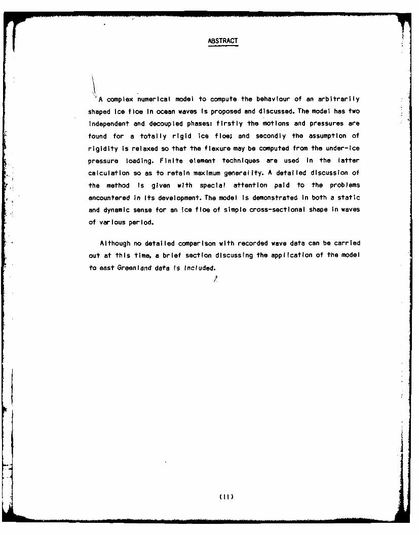
A complex numerical model to compute the behaviour of an arbitrarily

shaped ice floe In ocean waves is proposed and discussed. The model has two

Independent and decoupled phases: firstly the motions and pressures are

found for a totally rigid ice floe; and secondly the assumption of

rigidity is relaxed so that the flexure may be computed from the under-ice

pressure loading. Finite element techniques are used in the latter

calculation so as to retain maximum generality. A detailed discussion of

the method is given with special attention paid to the problems

encountered in its development. The model Is demonstrated in both a static

and dynamic sense for an ice floe of simple cross-sectional shape In waves

of various period.

Although no detailed comparison with recorded wave data can be carried

out at this time, a brief section discussing the application of the model

to east Greenland data is Included. A!

(ii)

ACKNOWLEDGEMENTS

I am indepted to Prof. Choung Lee of the Naval Ship Research and

Development Center in the United States for his dedication when

implementing the ship-motions program on the Cambridge computer. I also

wish to thank Dick Henshel I and Nell RIgby of PAFEC whose guidance enabled

the finite element model to be applied in a somewhat unconventional

manner. The fIeldwork reported in this article took place near Mestersvig

I n East Greenland, and I am grateful to Peter Wadhams and other members of

the Sea Ice Group for their efforts In making It a successful fieldprogramme. Finally I thank Dougal Goodman and Monica Kristensen for

helpful and critical discussion, and Rob Massom for his drafting skills.

This work was supported financially under Office of Naval Research

contract N00014-78-G-0003 and by the British Petroleum Co., Ltd. The

Natural Environmental Research Council of Great Britain provided salary

support for the author.

(IIl)

TABLE OF CONTENTS

PAGE

1. INTRODUCTION AND DISCUSSION 1

2. THE MOTIONS OF ICE FLOES IN WAVES 4

2.1 Introduction 4

2.2 MathematIcal Foundation of the Model 4

2.3 Simulation of the Motions of an Ice Floe 8

3. FLEXURAL BEHAVIOUR OF ICE FLOES IN WAVES 17

3.1 Introduction 17

3.2 The Sub-Ice Pressure Field 20

3.3 Preliminary Discussion of the Finite Element Model 21

3.4 App I Ication of the Method 26

3.5 DynamIc Anal ysis 38

4. PRELIMINARY COMPARISON OF THEORY WITH EAST GREENLAND DATA 47

4.1 Introduction 47

4.2 Resu Its of Compar i son 49

5. BIBLIOGRAPHY 55

II

(Iv)

1. INTRODUCTION AND DISCUSSION

Since 1959 when Gordon Robin used a ship-borne wave recorder aboard RRS

John Biscoe to measure waves in the Antarctic (Robin, 1963), the Scott

Polar Research Institute has been involved In studies relating to the

Interaction of ocean waves with pack ice. A series of papers and reports

have been published which have used novel techniques for studying

penetration of waves into fields of ice floes, and which have posed such

questions as: a) what happens to the open ocean energy spectrum as it

travels through pack ice; b) what effect do waves have on a particular

distribution and concentration of ice floes; c) how does an individual Ice

floe behave when subjected to ocean waves? These questions have led to

several in situ experimental programs which have taken place off

Newfoundland, in the Bering Sea, and in the Greenland Sea (see for example

Wadhams, 1973a, 1973b, 1978; Squire and Moore, 1980; Squire and

Martin, 1980; Moore and Wadhams, 1981). This work has been almost totally

experimental except for the model originally proposed by Wadhams in

his 1973 Ph.D. dissertation. Using a method devised by Hendrickson (1966),

with corrections for sign errors, Wadhams (1973b) approximated the Ice

floe as a thin elastic plate on deep water. By using a potential matching

method, he was then able to find approximate solutions for the waves

beneath and on either side of the floe. Unfortunately, the matching could

not be carried out perfectly and as Wadhams points out, there are

additional unknown potentials in each region which must be Included to

form the complete solution. The derivation of these potentials represents

a formidable task and no exact solution has been found to date even for

the lInearIsed equations. More recent work (Squire 1978) has concentrated

on another weakness of the early studies, namely in the modelling of the

material properties of sea Ice, rather than on the lack of sophistication

in the hydrodynamics.

Clearly, to be able to answer questions a) and b) above one must first

be able to answer question c) since the behaviour of the component ice

floes must control the dynamics of the complete Ice field. The matched

Section 1 1 Introduction

potential approximation is inadequate If one wishes to Include all the

motions (including bending) of the !ndividual ice floes, but nonetheless

has provided a reasonable fit to experimental data collected over the ice

pack as a whole. Current interest has, however, been centred around the

determination of the characteristics of motion and flexure of a solitary

Ice floe in waves. For this problem, the matched potential approximation is

grossly in error and predicts unrealistic values for the wave generated

loads and motions. Two consecutive field seasons in east Greenland waters

have been carried out with the prime objective of measuring the dynamics

and flexing of discrete ice floes under wave loading. Surface strain, heave

and sway were measured aboard several floes of different shape and

dimensions, and the waves in the open water near the floes were recorded

during the experiment. The two seasons were both extremely successful and

have produced a data base which has been analysed during the last year to

produce power spectra, frequency response functions between forcing and

response, etc. The results have prompted the present study, whereby a

theoretical model which is able to compute all the motions of an ice floe

as well as its flexural behaviour without the approximations Involved in

potential matching, has been developed. The model is numerical throughout

due to the complexity of the mathematics.

During the analysis of the east Greenland dataset, the author carried

out an extensive survey of the literature relating to the mathematics and

physics involved in the interaction of waves with sea Ice. The problem for

an Individual floe is not unlike that encountered by naval engineers who

are interested in the motions and bending of ships at sea. The modern

history of this subject began with Ursell (1949 a), who formulated and

solved analytically the complex mathematics which arise when a semi-

Immersed circular cylinder is allowed to move sinusoidally In a fluid.

Subsequent work general Ised Ursel I's cross-section to shapes of particular

Interest to ship designers. Much more recently, the problem has been

reformulated so as to be suitable for solution by numerical methods. In

principle this enables all the motions of a body of arbitrary shape In

waves to be computed, so that from the naval engineers viewpoint the

problem is essentially solved.


Despite the obvious similarities between our problem and that of ship

design and engineering, there are very important differences. A naval

engineer asks different questions and requires accurate estimates of

particular parameters which are not necessarily of Interest in the present

study. Furthermore, the mechanical properties of sea ice and steel are a

world apart so that whereas the rigid body approach may well suffice for a

mathematical model of a ship in waves, it certainly would not suffice for

an ice floe. For this reason very little work of suitable application

could be found on wave induced flexure of ships, so that the author chose

to take a novel approach which still allowed any cross-section shape to be

analysed.

In this report we will lay down the framework of a method which can be

used to compute both the wave-induced motions and the bending for any

floating object in waves. The discussion is naturally directed towards

calculating the response for ice floes since this was the problem

originally posed. The model is equally applicable to any floating or

submerged body in waves however, so that the method is far more general

than this work indicates. In -edition to our ice floe studies we have

already been able to use the model to compute the motions of a large

tabular iceberg. The calculations show resonances in heave, roll and

strain which are also observed in field data obtained during a recent

Antarctic field season.


2. THE MOTIONS OF ICE FLOES IN WAVES

2.1 Introduction

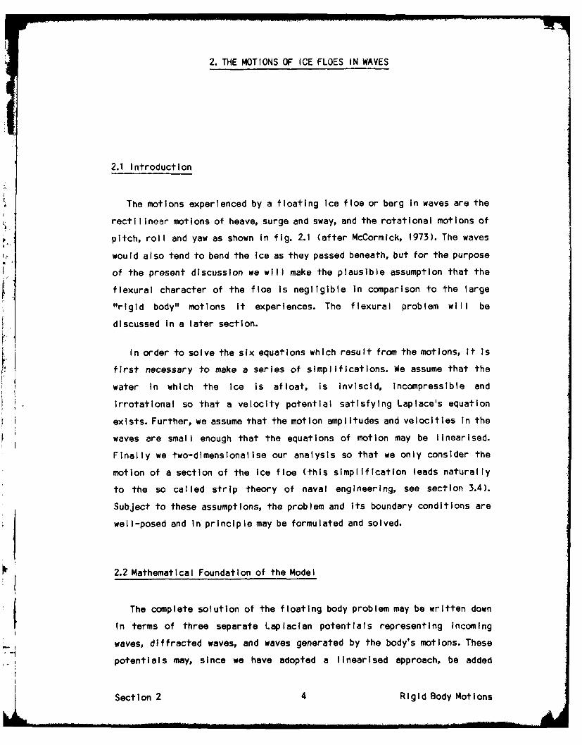
The motions experienced by a floating Ice floe or berg in waves are the

rectilinear motions of heave, surge and sway, and the rotational motions of

pitch, roll and yaw as shown in fig. 2.1 (after McCormick, 1973). The waves

would also tend to bend the ice as they passed beneath, but for the purpose

of the present discussion we will make the plausible assumption that the

flexural character of the floe is negligible In comparison to the large

"rigid body" motions it experiences. The flexural problem will be

discussed in a later section.

In order to solve the six equations which result from the motions, it is

first necessary to make a series of simplifications. We assume that the

water In which the ice is afloat, is Inviscid, incompressible and

Irrotational so that a velocity potential satisfying Laplace's equation

exists. Further, we assume that the motion amplitudes and velocities in the

waves are small enough that the equations of motion may be linearised.

Finally we two-dimensionalIse our analysis so that we only consider the

motion of a section of the Ice floe (this simplification leads naturally

to the so called strip theory of naval engineering, see section 3.4).

Subject to these assumptions, the problem and Its boundary conditions are

well-posed and In principle may be formulated and solved.

2.2 Mathematical Foundation of the Model

The complete solution of the floating body problem may be written down

I n terms of three separate Laplacian potentials representing incoming

waves, diffracted waves, and waves generated by the body's motions. These

potentials may, since we have adopted a linearised approach, be added

Section 2 4 Rigid Body Motions

*U x

44

wJ w

0 *1w

> LL.

xIw~

Secton 25 Riid Bdy Mtion

together to create the velocity potential which represents the total fluid

disturbance. Many of the analytic solutions in the literature are

concerned with the evaluation of the wave-making potential since in

laboratory experiments one wishes to know exactly how a particular wave

flume behaves hydrodynamically (see for example Ursel , 1949a, 1949b). The

difficulty arises when the complete potential for the floating body

[ problem Is required, and various other simplifications have been employed

by naval engineers for the motion of ships In waves.

When a body undergoes motion wIthIn a fluid it behaves as though it has

increased Inertia or mass (Lamb, 1962). This Is a hydrodynamical effect

known as added mass which for cyclic motions will be frequency-dependent.

Furthermore, the oscillating body will use energy In creating and

maintaining the outgoing waves It generates. This leads to a frequency-

dependent damping force in our system of equations. The evaluation of both

added mass and damping for arbitrary shaped bodies, at various incident

wave periods, is extremely complex. Also the calculation of the diffracted

wave potential poses difficulties for all but the simplest of geometries.

There is motivation, therefore, for simplifying the equations of motion by

neglecting the above quantities. A selection of possible approximations

which could be used to model the motion of ships In waves are discussed in

detail by Lee (1976). Lee choses to consider five possible cases: a) added

mass, damping and diffraction are neglected; b) damping and diffraction

are neglected and the added mass is set at the displaced fluid mass; c) as

previous case except that diffraction is included; d) added mass and

damping are treated correctly but diffraction is neglected; e) complete

theory. The assumption that diffraction effects may be omitted is

sometimes known as the Froude-Krylov hypothesis, and is equivalent to the

supposition that the motions of the body do not alter the particle motions

of the fluid although the particle motions Influence the body. Lee carried

out the analysis for both floating and submerged bodies, and found in the

former case that the inclusion of frequency-dependent added mass and

damping were essential, and that with no diffraction the computed results

(for the sections he chose) were between 20% and 30% in error. For Ice

floes in waves therefore, it Is Important that no such approximations be

made.


There are two procedures which have commonly been used to !.olve the

floating body problem. The first of these, known as the multipole expansion

method, was originally developed by Ursell (1949a) for circular cylinders,

and was later applied to sections of arbitrary shape using conformal

mapping (the Theodorsen transformation). The second, and more recent

technique, represents the problem by a Fredhoim integral equation of the

second kind, and then approximates that equation by a system of linear

algebraic equations. Other procedures exist and are described In detail in

an excellent review by Wehausen (1971). The present author's work utilizes

a computer program based on the second method.

The program to model floating bodies in waves was originally developed

by Frank (1967). Frank approximated the body's cross-sectional contour

with a number of nodal points joined by straight line segments. He then

used the complex source potential of Wehausen and Laltone (1960), subject

to an additional velocity boundary condition across the cylinder's

surface, To derive a pair of integral equations. By assuming that the

source strength varied from segment to segment but was constant along each

segment, Frank was able to write down a set of linear algebraic equations

which could be solved numerically. The advantage of thIs method over the

multipole method is that many terms are required in the Theodorsen mapping

to treat bodies of non-simple cross-sectional shape. Initial problems

concerning wave periods at which no solution to the Integral equation

exists (John, 1950) and bodies of unsuitable section, have now been

overcome (C.M. Lee, personal communication, 1980).

The modified version of the program originally developed by Frank has

been implemented on the IBM 370/165 computer at the University of

Cambridge. Prof. C.M. Lee of the Naval Ship Research and Development Center

In Washington D.C., and the present author encoded three versions of the

program; one to derive reflection/transmIssion characteristics of

symmetric ice floes, one to compute the motions of an asymmetrIc body, and

one which included a viscous roll damping which was particularly directed

towards Iceberg problems. The latter two programs use extended precision

arithmetic but still typically run within a few seconds CPU time per wave

frequency. The program has been tested many times for various cross-

sectional shapes and compares well with experimental results (see for


example Frank, 1967; Lee, 1976). With this in mind the author does not

propose to repeat these tests, Instead we wi II run the program for an Ice

floe of realistic dimensions in waves of typical period, and will

qualitatively discuss the results by comparing with laboratory

experiments in the literature.

2.3 Simulation of the Motions of an Ice Floe

In this, and In subsequent sections, we shall consider an ice floe of

typical east Greenland dimensions, viz. 20m beam by 3m thickness. The Ice

* floe will be assumed to be of simple rectangular shape with a density of

922.5 Kg m-3. Neither the shape nor the dimensions are significant and any

Ice floe whose cross-section Is a simply connected region and which could

adequately be represented by Frank's polygonal approximation, could be

modelled. The ice floe is now assumed to be acted apon by waves between Is

and 20s period. The amplitude of these waves is normalised to Im so that

any plots of heave, sway or roll magnitude may be thought of as the

amplitude of the frequency response function for the floe, and plots of

pressure are specific to that amplitude. Furthermore, the Incident waves

are assumed to be beam-on to the ice floe in all cases so that only heave,

sway and roll motions will be non-zero.

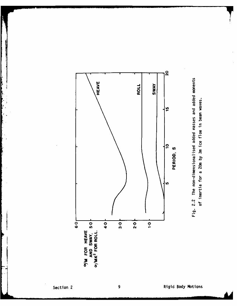
We begin in fig. 2.2 by plotting the added masses for heave and sway,

and the added moment of inertia for roll. The added masses have been non-

dimensionalised by division by the mass of the fluid displaced by the

floe, and the added moment of inertia with respect to that mass multiplied

by the radius of gyration about the centre of roll. Both the added mass and

the added moment of Inertia curves compare well wIth those computed by

Vugts (1968a) for various cross-sectional contours. There is the same

characteristic Increase in added mass for heave as period Increases, and

the same minimum at some point defined by the body's shape, indicating as

we suspected, that any theory which neglects the dependence of added mass

on frequency would be unacceptable. The added mass for sway and the added

moment of inertia for roll show little dependence on period except for

short period waves.


~~*~~-0N

-J4I

WU 0

0>

00

0

uC.4

L.

00

60 LA0

0.. ZC~

Secton 29 Riid Bdy Mtion

EmA

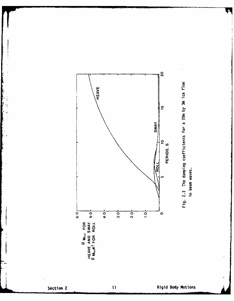
The various damping coefficients plotted in fig. 2.3 have been non-

dimensionalised in a similar way to the added mass curves, with the

addition of an extra factor representing the radian frequency of the

incoming waves. These plots may also be compared qualitatively with those

found in Vugt's paper. The same characteristic maxima In the sway and roll

curves are apparent, but Vugt's heave curves have a maximum. On closer

examination we find that the dependence of heave damping on frequency is

considerably influenced by the draft/thickness ratio of the floating body;

as draft increases so the maximum decreases and moves towards increasing

period. None of Vugt's cross-sectional shapes have similar draft ratios so

are inappropriate for comparison. A close representation of our ice floe

is to be found in Frank (1967) where the heave damping ratio is presented

for a rectangular section with rounded corners and significant draft.

Frank's curve shows exactly the same behaviour as that in fig. 2.3.

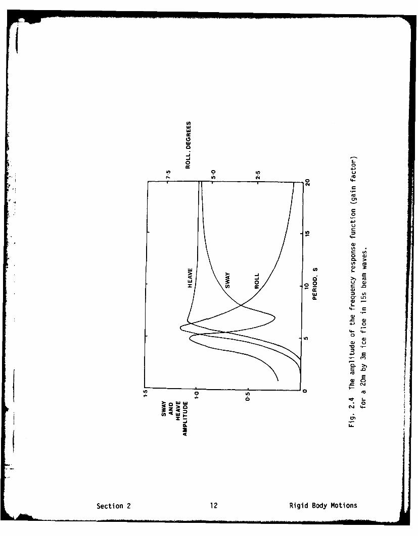
Having computed the added mass and damping coefficients as a function

of period, we are now in a position to evaluate the wave amplitude ratios

due to heave, sway and roll (fig. 2.4). Each of these curves shows a

distinct resonance which occurs at a wave period which is quite likely to

be found in a open ocean wave spectrum, particularly for an under-

developed sea. At a resonant period, the body would tune to the waves so as

to produce an enhanced heave, sway or roll magnitude. For long waves, as

one might expect, the heave and sway amplitudes tend to unity indicating

that the body is simply following the particle motions at the wave

surface. Likewise, the roll magnitude becomes small. As one decreases in

period, so the response of each motion becomes more complicated: the heave

and roll resonate and then decrease so that for waves of less than about

4s periods these motions wilIl not be excited; and the sway magnitudedecreases to a minimum at about 7s, resonates at around 5s and then also

decreases. The complex shape of the sway curve is interesting since it

means that for our ice floe one would expect to see enhanced or suppressed

component motions at certain wave periods. The shape of the curves Is

sImIlar to those measured by Vugts (1968b).

An interesting effect described in that paper is found when the phase

difference between roll and sway is computed as a function of wave period.

This calculation has been carried out and Is shown In fig. 2.5. At a period


0

LG)0

'I-

CV)o

in

.0

0 44-0

Ej uM Im

LA-

0 0 0 0 0 0

(D C C

>:--

0 < -0

in

2~ a,0

Section 2 1Rgid Body Notions

"-- " "....... . . . . . .. . . l/I .... . ... • "' .. ... . ....... . I l3

w

w

0a

CL >

j S

oE

0 0

.g )

4 0

E

CL

Qt C

x Cdi0L.

Secton 12 igi Bod Moins

0

CYC

0

,0

.0.

0

(J)

04- Eo

4-

N- V- V-

°a-

J.

i . p p p p I i i

S33:91:1 '33N3I:i 3SVHd


which appears to correspond to the minimum in the sway amplitude ratio

curve, the phase difference rapidly changes through 180 degrees. Vugts

found this phase change experimentally for various rectangular sections

and in each case the phase altered rapidly near the sway minimum. At low

periods therefore, our roll and sway are in anti-phase, whereas at longer

periods they are in phase. Fig. 2.5 illustrates the complicated nature of

the coupling which exists between roll and sway.

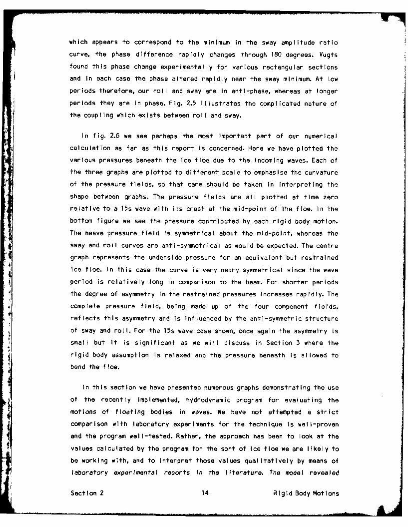
In fig. 2.6 we see perhaps the most important part of our numerical

calculation as far as this report is concerned. Here we have plotted the

various pressures beneath the ice floe due to the incoming waves. Each of

the three graphs are plotted to different scale to emphasise the curvature

of the pressure fields, so that care should be taken in interpreting the

shape between graphs. The pressure fields are all plotted at time zero

relative to a 15s wave with its crest at the mid-point of the floe. In the

bottom figure we see the pressure contributed by each rigid body motion.

The heave pressure field is symmetrical about the mid-point, whereas the

sway and roll curves are anti-symmetrical as would be expected. The centre

graph represents the underside pressure for an equivalent but restrained

ice floe. In this case the curve is very neary symmetrical since the wave

period is relatively long in comparison to the beam. For shorter periods

the degree of asymmetry in the restrained pressures increases rapidly. The

complete pressure field, being made up of the four component fields,

reflects this asymmetry and is influenced by the anti-symmetric structure

of sway and roll. For the 15s wave case shown, once again the asymmetry is

small but it is significant as we will discuss in Section 3 where the

rigid body assumption Is relaxed and the pressure beneath is allowed to

bend the floe.

In this section we have presented numerous graphs demonstrating the use

of the recently implemented, hydrodynamic program for evaluating the

motions of floating bodies In waves. We have not attempted a strict

comparison with laboratory experiments for the technique is well-proven

and the program well-tested. Rather, the approach has been to look at the

values calculated by the program for the sort of Ice floe we are likely to

be working with, and to Interpret those values qualitatively by means of

laboratory experimental reports In the literature. The model revealed


*1915 CMLT

19-14 PRESSURE

19-13

19-12

19-10

1909

17-5

-174

S173EZ 17-2

wi 17-1

S170CRESTRAINED

169 -ICE FLOE

*1681

3-0

0

2 4 6 8 10 12 14 18 18a 20

DISTANCE ALONG ICE FLOE. m

$ Fig. 2.6 The component and the complete pressure fields beneath

a 20m by 3m ice floe due to 15s beam waves. Note the scale

change in the pressure axis.

!Ri! _B vat

structure that could not have been predicted without an intensive series

of scaled laboratory or field experiments, which would be prohibitably

expensive. The existence of resonant peaks within the bandwidth of a

typical open ocean spectrum is extremely relevant since this would

considerably influence any experimental values measured aboard the ice

floe. The anti-phase/in-phase relationship of sway and roll is also very

interesting and is worth investigation under field conditions by means of

tiltmeters and sway accelerometers


3. FLEXURAL BEHAVIOUR OF ICE FLOES IN WAVES

3.1 Introduction

In the first part of this article we discussed and demonstrated a

powerful method for evaluating the rigid body motions of an ice floe or

iceberg subjected to incoming waves. The numerical method was able to cope

with an arbitrarily shaped two-dimensional section of the body and compute

five out of the six rigid body modes. The sixth mode, surge, has little

effect on the pressure beneath the floe so can safely be neglected without

undue loss of accuracy. In this section we aim to relax the fundamental

assumption of rigidness and allow the floe to bend as the wave propagates

beneath. The basis of our entire analysis is the hypothesis that to first

order, the flexural behaviour and the rigid body behaviour may be

decoupled. As far as the fluid is concerned, this is equivalent to saying

that the particle motions beneath the wave profile do not feel the body

bend. Thus, from a hydrodynamical point of view, our assumption is

extremely reasonable since typical flexural displacements lead to

extremely small floe curvatures which can have negligible Influence on the

fluid motions. Certainly the more important consideration is, what is the

effect of decoupling our calculations as far as the Ice floe's response is

concerned? Essentially, the wave-ice Interaction problem is a resonance

problem (R.E.D. Bishop, personnal communication, 1981 ) so that feed back

mechanisms between flexural and rigid body behaviour are not necessarily

negligible particularly close to natural frequencies of oscillation or

flexure. Naval architects have for many years tended to overlook these

problems and have obtained quite reasonable results with relatively

simple models (often assuming the Froude-Krylov hypothesis). We proceed

with our more complete but decoupled solution with this in mind.

Comparisons of our model with real data are regarded as the ultimate test

of the decoupling procedure and will be carried out in a later paper. A

prelimInary comparison of data and theory is presented In section 4.

Section 3 17 Flexural Motions

The rigid body program described earlier is not restricted in any way

to simple geometrical cross-sections. As long as the Ice beneath the

waterline can be effectively modelled by a topologically simple curve, and

hence by a collection of points on that curve, the program may be run and

the modes and sub-ice pressures computed. It is clearly possible to then

use these pressures to find the strain at the surface of a floating ice

floe by means of a thin plate analysis (Timoshenko and Woinowsky-

Krieger, 1959). The author began this work by adopting such a procedure. An

elementary computer program was written based on the Duhamel integral

method of Timoshenko et al (1974) and discussed more fully in

Goodman et al (1980) with reference to ice islands and ice floes. The

program is capable of computing the strain as experienced by a strain

gauge located anywhere along the floes upper surface. Good agreement with

observations for thin floes was obtained though the discrepancies between

theoretical and measured strain became significantly worse as the

thickness increased.

In many ways a thin plate theory is a step backwards since we have been

forced to restrict a very general model to the oversimplified geometry of

a thin plate. By doing this we have destroyed any capability of solving

more interesting problems such as: how does a floe with a sill or an

undercut bend on waves; what effect would a keel beneath the floe have on

its total response; how would a cracked floe respond; etc. If we want to

solve such problems, it is clear that no amount of analytical work will

yield solutions for floes of such arbitrary shape and specification. We

are forced to turn to numerical methods.

There are two popular numerical procedures by which this sort of

problem may be solved. Both are extremely general and both could well be

used to compute stresses and strains etc. for arbitrary shaped floes given

some pressure loading. Both methods have well-defined advantages and

disadvantages.

$ The first method historically is that of finite difference analysis,

whereby the partial differential equations for the problem to be solved,

and its boundary conditions, are expressed in their finite difference

forms. A matrix equation may then be constructed and solved by means of

Section 3 18 Flexural k* ions

some sort of iterative procedure such as successive over relaxation or an

equivalent technique. The main drawback of this method is that it is

difficult to generalise to arbitrary geometries since by its very nature,

the matrix equation set up Is specific to the geometry and the grid

pattern chosen. This implies that any finite difference analysis tends to

be very problem specific.

The second and more recent method was developed with the advent of

large main-frame computers. In this technique, known as finite element

analysis, the body is replaced by a "patchwork" continuum of smaller

bodies with exactly the same physical properties. The choice of the word

"patchwork" is deliberate for it emphasises the fact that each element has

the same characteristics as the complete body. These elements are assumed

to be interconnected along their boundaries at a discrete number of nodal

points whose displacements prescribe the displacement of the element as a

whole. By expressing the element's state of deformation (or strain) in

terms of a uniquely defined displacement function, and by considering the

appropriate nodal forces, boundary stresses and distributed loads, It is

then possible to write down the so-called stiffness relations for each

element and hence for the entire body. Clearly there are certain

topological restraints which should be applied to the continuum since

overlapping of elements or their separation to form holes or cavities

cannot be permitted. Unfortunately, such restraints imply continuity of

nodal displacements between elements which can only be satisfied in the

limit of an infinitesimally fine discretlzation, so that a degree of

approximation is inherent In the finite element technique. The matrix

equations formed in this way may be solved to give the body's

displacements, strains or stresses by one of the standard numerical

procedures. For a more detailed description of finite element methods the

reader Is referred to Desal and Abel (1972) or Zlenklewlcz (1972). It is

this method that the author has chosen to model the ice floe in waves

problem.


3.2 The Sub-Ice Pressure Field

Throughout this work we will assume that our ice floe is of simple

rectangular cross-section. Typical east Greenland floe dimensions of 20m

across by 3m thickness are chosen as before though of course the

simplicity of the geometry and the particular dimensions chosen are

unimportant. With this model, a rigid body calculation as described in part

I of the report may be carried out and the pressure field computed beneath

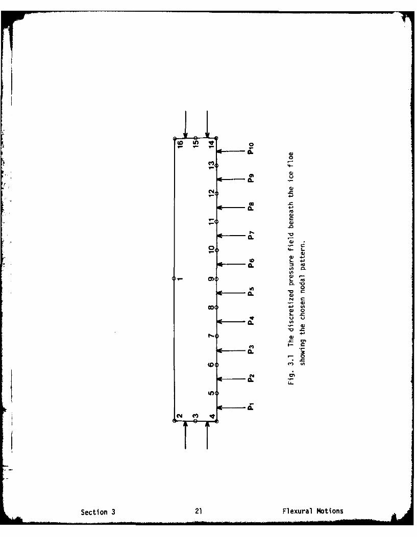
the floating ice floe for a variety of incident wave periods. For a 20m

ffloe, 16 nodal points will produce the pressure field as shown in fig. 3.1.

The i ce flIoe can then be all Iowed to bend to th is pressure f ielId.

From the point of view of surface strain, the edge pressures will have

little effect on an instrument located near to the centre of the floe. The

edge pressures are therefore neglected for the present analysis. Indeed,

these pressures will very nearly cancel one another out as far as the

rigid body part of the calculation is concerned (in a symmeterised

analysis they would be equal and opposite). The pressures beneath the floe

are defined at isolated positions along its underside, but none-the-less

they must represent a smooth and continuous upward pressure distribution.

This distribution will be slightly asymmetric in a complete analysis since

one would expect the wave to be effected by the ice floe. It would be quite

feasible to use the sampled pressure field to solve the bending problem.

However,such a grid spacing would be extremely coarse and would no doubt

produce unacceptable accuracy when the computation was carried out. For

this reason, the author has chosen to use the sampled pressure to

regenerate the "original" distribution by means of interpolation. The

method employed for this reconstruction is a well-tested numerical

technique which creates an interpolate curve by patching together a series

of cubics. The interpolate Is continuous and has continuous first

derivatives. By this method, the upward loading due to the static wave

profile may be found at any point along the underside of the ice floe. In

principal the loading may then be applied to a finite element model and

the resulting displacements and principal stresses found.


m o

0M() #4--

IL~U

4)

a.

a. -

.e-

4-

ec 4-)

(1) 0

CN

N- a

Section~~~4 3 1FexrlNoin

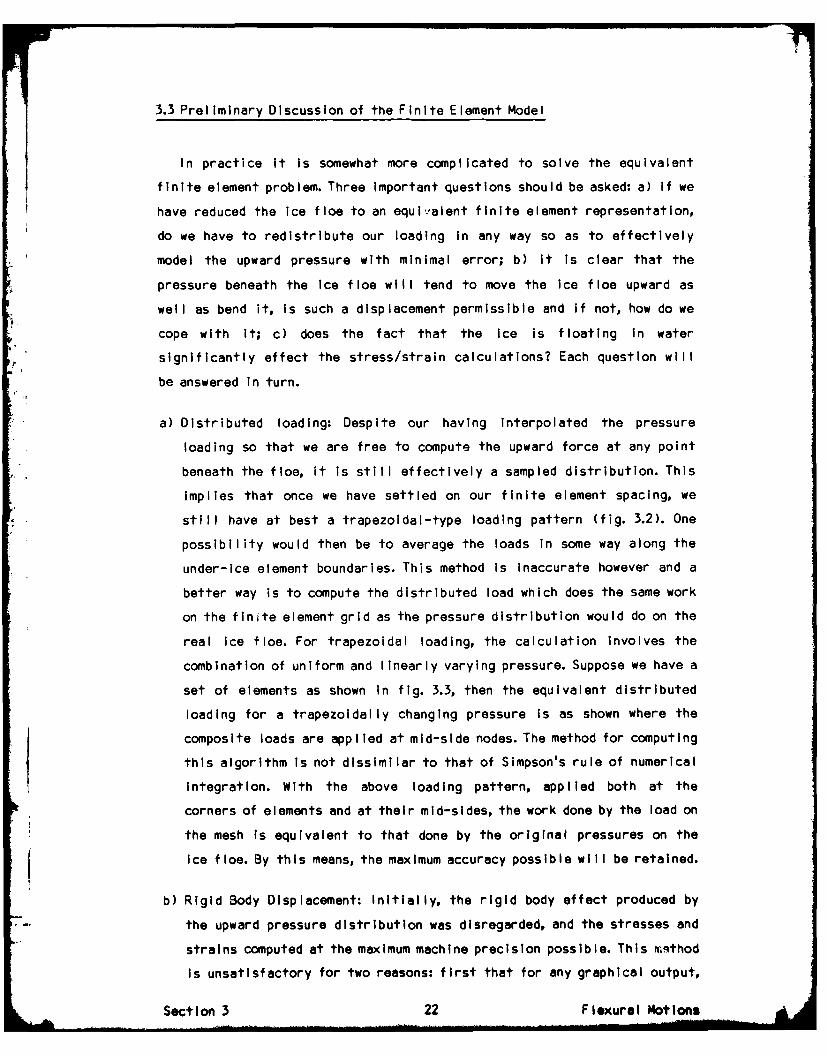
3.3 Preliminary Discussion of the Finite Element Model

In practice it is somewhat more complicated to solve the equivalent

finite element problem. Three important questions should be asked: a) if we

have reduced the ice floe to an equivalent finite element representation,

do we have to redistribute our loading in any way so as to effectively

model the upward pressure with minimal error; b) it is clear that the

pressure beneath the Ice floe will tend to move the ice floe upward as

well as bend it, is such a displacement permissible and if not, how do we

cope with it; c) does the fact that the ice is floating in water

significantly effect the stress/strain calculations? Each question will

be answered in turn.

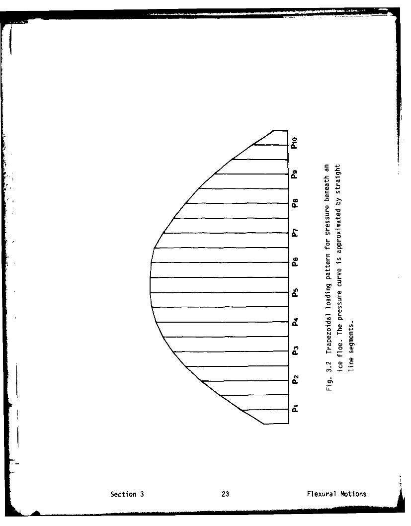
a) Distributed loading: Despite our having interpolated the pressure

loading so that we are free to compute the upward force at any point

beneath the floe, it is still effectively a sampled distribution. This

implies that once we have settled on our finite element spacing, we

still have at best a trapezoidal-type loading pattern (fig. 3.2). One

possibility would then be to average the loads in some way along the

under-ice element boundaries. This method is inaccurate however and a

better way is to compute the distributed load which does the same work

on the finite element grid as the pressure distribution would do on the

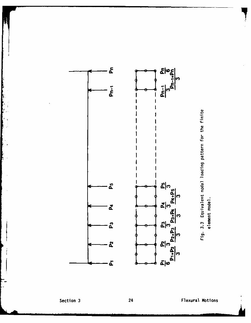
real ice floe. For trapezoidal loading, the calculation involves the

combination of uniform and linearly varying pressure. Suppose we have a

set of elements as shown in fig. 3.3, then the equivalent distributed

loading for a trapezoidally changing pressure is as shown where the

composite loads are applied at mid-side nodes. The method for computing

this algorithm is not dissimilar to that of Simpson's rule of numerical

integration. With the above loading pattern, applied both at the

corners of elements and at their mid-sides, the work done by the load on

the mesh is equivalent to that done by the original pressures on the

ice floe. By this means, the maximum accuracy possible will be retained.

b) Rigid Body Displacement: Initially, the rigid body effect produced by

* -the upward pressure distribution was disregarded, and the stresses and

strains computed at the maximum machine precision possible. This nthod

is unsatisfactory for two reasons: first that for any graphical output,

Section 3 22 Flexural 14otionsA & . . . . i i l lll . . .I .. . . . . . i . . . .. . . . . . . . . . . .." . .- - "

0 4-)

CL0o a.

4-) 0.

4J 0E

-~ >

0. -.

o o.

=4J

U)-4-.

a)4A2

n

.U

Secio 3- 23Feua oin

tOh. 0

So 0' 4-0.

*r0

| ......

CC

0+_

CL II

4--

+ CO 4-)

C ':

V I O 0

a.~

+ LLJ C1S na oto

CL> 0

+ ~ .IC4~..C


the bending is buried within the much larger rigid body translations;

and secondly that computing time substantially increases when maximum

precision is used throughout. It was soon clear that some alternative

procedure was necessary. R.D. Henshel I (personnel communication, 1981)

suggested that either the rigid body part of the loading should be

removed so as to produce an Integrated load which did no work on the

ice floe, or an enhanced gravity field should be applied so that the

total upward pressure was opposed exactly by the downward body forces.

The first method is by far the simpler to implement routinely so that

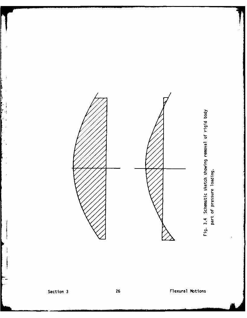
the present author has adopted that method. The original and the

transformed pressure distributions are shown schematically in fig. 3.4

where in the second diagram the shaded area must sum to zero. When this

procedure Is implemented, Increased precision computation can be

limited to the displacement calculations alone, and the stresses and

strains may be found using less computer time and machine storage.

c) From a common sense viewpoint, the fact that the ice is afloat must be

significant since without the presence of the underlying water, an

unrestrained ice floe would simply move skyward an indefinite amount

under upward loading. One solution might be to restrain the body at

some node within the finite element mesh. Such a procedure would yield

reasonable bending displacements but introduces unrealistic stress

concentrations near the constrained node and is therefore

unsatisfactory. A better procedure would be be to consider exactly what

happens when a floating body is forced upwards by a small distance.

Suppose that our ice floe is raised by an amount 6 , then an opposing

pressure of magnitude Pwg 6 will act so as to restrict translation.

This implies that the water beneath the floating body is behaving as aspring with modulus equal to pwg. We say that the ice Is behaving asthough bonded to an elastic foundation of modulus owg. Returning to

the finite element model, therefore, we represent the flotation part of

the problem by connecting a series of grounded springs to the elements

on the underside of the ice floe. The equivalent distribution of

springs (so that the spring loading does the same work on the finite

elements as would the real buoyancy forces on the floe) is computed by

assuming a uniform downward loading of the mesh.

Section 3 25 Flexural Motlons

U-v

0

r .r.

Foo,

°-

0

Secton 326 lexual Mtios

We have discussed three basic questions which are encountered when the

finite element method is applied to ice-wave interactions. We may now

proceed with a more detailed discussion of the method employed.

3.4 Application of the Method

By its very nature the rigid body calculation discussed in the previous

section is a two-dimensional strip theory. That is to say that if three-

dimensional results are required, the body is assumed to be made up of two-

dimensional elemental strips or cross-sections which may be totally

decoupled from one another. The program may then be run for each cross-

section and the results integrated so as to simulate a three-dimensional

floating body. The strip theory has been fully tested over the years and

has proved reliable in computing the rigid body behaviour of a variety of

underwater forms. Indeed, there is little justification in developing a

fully three-dimensional theory since the theoretical and the measured

results show excellent agreement (C.M. Lee, personnal communication, 1980).

When one allows the body to bend under the wave loading however, the

effectiveness of a two-dimensional model is not nearly so well-defined.

The author knows of no equivalent technique which has been compared with

experimental data in any way, so that although it is tempting to treat the

bending as a strip theory, such a step must be regarded as an untested

hypothesis. It should also be noted that whereas the reduction of the full

three-dimensional rigid body analysis to a series of two-dimensional

strips is conceptually easy to grasp, particularly for beam waves, this is

not the case when a body is allowed to bend. In general, stress and strain

are tensorial quantities and when simplification is made into a planar or

cross-sectional analysis, care must be taken in both defining the problem

and in interpreting the results. This is particularly true when icebergs

are consi.dered since all three dimensions are of comparible magnitude. It

is important to appreciate that the behavior of a two-dimensional section

Is not the same as that of an equivalent plate of arbitrary thickness. The

first case is a problem of plane strain whereby any displacement Into the

third dimension Is assumed to be zero, and the second case would be solved

as a plane stress problem so that the components of stress Into the plate


thickness would vanish. Our cross-sectional strip of ice floe should be

solved in plane strain which fortunately leads to a very simple

relationship between the principal stresses al,a2 and the principal

strains C1, C2 material (Jaeger, 1956), viz.

oz = (X+2G)c + Xe 2,

02 = (X+2G)c 2 + AE1 ,

where X and G are Lame's parameters, and the convention that the

subscripts 1 and 2 imply greater and lesser principal components will be

used. For icebergs however, the plane strain assumption could lead to

serious errors if the length, breadth and thickness are similar, and

strictly a completely three-dimensional approach should be adopted. With

the limitation of a two-dimensional rigid body strip theory, this might be

carried out in three stages: first the iceberg is considered as a series of

cross-sectional shapes and the pressure loading is calculated for each

section; then an interpolate surface is fitted to the pressures in a

similar way to the pressure curve found In our two-dimensional study;

finally the pressure surface is used as areal loading in a three-

dimensional finite element model. The author does not propose to

demonstrate the use of this technique in this report since we are

primarily concerned with ice floes.

The numerical scheme for carrying out the finite element analysis was

developed by PAFEC Ltd. In the U.K. It consists of a suite of user

orientated Fortran programs capable of dealing with a variety of

engineering-type problems and in principle may be used with little

difficulty once the fundamentals of finite element modelling are

understood. It is fair to say that we have used finite element modelling in

rather an unorthodox way; we have applied a very powerful engineering

technique to a complex geophysical situation. All the difficulties

encountered have been conceptual rather than fundamental.

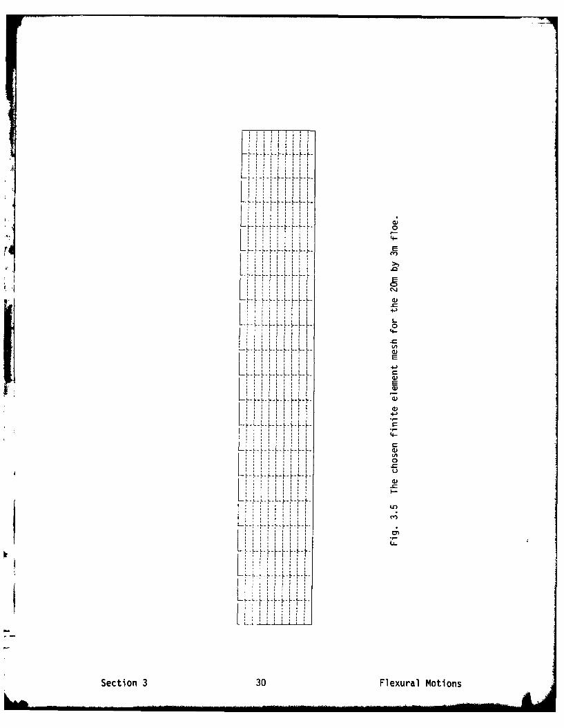
A suitable grid pattern for our 20m by 3m ice floe was set so as to take

advantage of the geometric simplicity of the original rigid body nodal

pattern. Twenty elements were chosen to represent the floe lengthwise and

ten elements through its thickness. Tests with finer grids showed little


improvement in accuracy. The finite element mesh is shown in fig. 3.5.

A preliminary numerical simulation was carried out by reducing the

dynamic loading to a static profile defined at the time of maximum

bending. This is by no means a trivial step especially for short period

waves, since there exists a phase lag between the original wave passing

beneath the floe and the resulting pressure distribution. When comparing

waves of different periods, therefore, care must be taken to ensure that

the computed strains have been calculated relative to equivalent parts of

the loading. If the pressure distribution were a simple sinusoid it would

be a simple matter to apply the necessary phase shift. For complicated

pressure fields however, we require some criterion by which to decide how

much the phase should be altered so as to standardise the flexure. The

method adopted uses a finite difference Iterative procedure to compute

maximum numerical curvature at the centre of the floes upper surface as

the wave moves relative to the floe. The wave is then shifted by the phase

necessary to attain this curvature. The phase shift for long period waves

is negligible but as the period decreases so the phase change becomes more

significant. After this phase translation has taken place, the maximum

stresses and strains would be found near the centre of the top of the ice

floe.

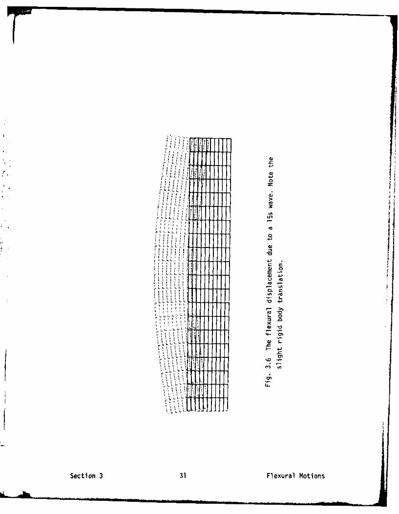
The static analysis has been carried out for several wave periods in

the range 5s to 25s passing beneath our 20m by 3m floe. For a 15s wave, the

loading is close to being symmetric but as can be seen in fig. 3.6, the

asymmetry of the under-ice pressures Is sufficient to slightly tip the ice

floe on the wave. Fig. 3.6 shows the resultant displacement of every point

in the finite element grid representing the floe. Clearly there is

significant bending and, as one might expect, the maximum bending

displacement is to be found at the centre of the floe's upper surface.

Returning to the apparent rigid body rotation in the figure, we see that

the angle of inclination is less than one second of arc which seems quite

reasonable for the initial asymmetric pressure pattern.

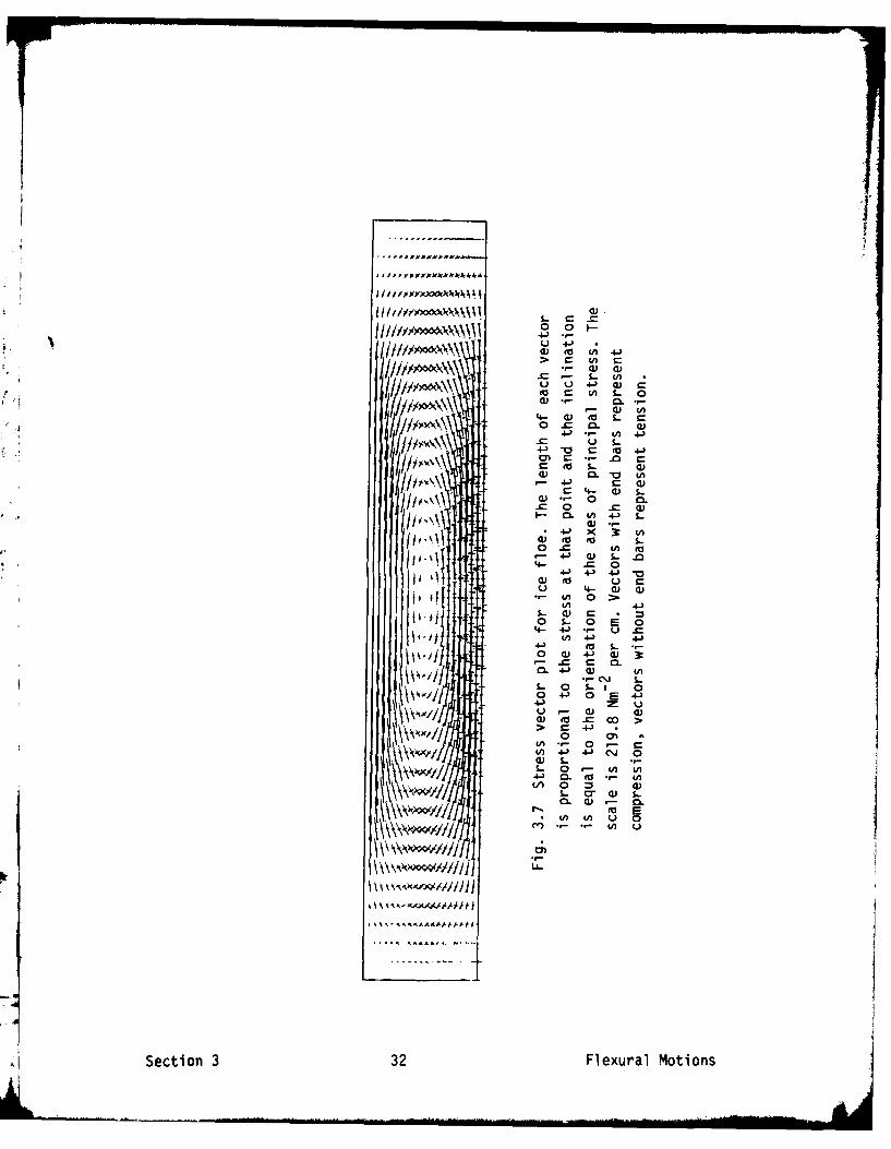
Having computed the displacements, we are now in a posItion to find the

stress or strain field within the Ice floe. Perhaps the simplest way of

visualisIng stresses Is by means of a stress vector plot. In fIg. 3.7 the


* a I a a i i

L- LL--L-LL-L.

,,I2

LLLLL

p . ' I I I

L -L- -~ L -L.-L

L L L L L L-L.LL. LL- -L.L L.L. 0

LLLL LL in

l l I

iS1 ii3

LL-K L.L-L-L-L.

I

-[ --lu -- i --l "

Secton 330 Fexurl Moion

L L L 0) i I I

r LL!

L. L L L I L 4

* ' i i , , 0 J

r CL

.C LLLtogtI I '? I $

rL L L L i .4.)

r L

I ! i I 0

r - s i iL i i-

l i' ii "0• LLLL .-.....

w V-

S t I3 1 F r o

Iii liii ,,I ,, .it,'

ill ....

... . ,. .,,.

CIUi 4-'

r C

*." w -

4J 4JCi 4 St

0" CL

4-"0 U" C

- ) 4-)

J 4- J 4 J

0 - . U

L) CJ4 - C ' 4-

S .- 0 0

III,- ) 0.o =J.C 4-A -)

0) 0 0 .C

I- 0. 0

-- X ,3 0

0ciC 4F u M i

- 4-' U 4J .0

o~f -.. - 0 t/) 4.=

LU) Cr W sM'J0 1 0 0x

(A-4A U 0Ciijt~( UA4'

-- 4- '.L .

Section 3 32 Fleura Mtin

vectors shown have a length which is proportional to their magnitude and

are plotted with the correct angular translation. Both principal stresses

are shown with the convention that compressive stresses are drawn with end

bars whereas tensile stresses are not. The principal stresses form the

pattern that one would expect for a simple body of this sort. We see

extensional stresses above the neutral axis and compressional stre,;ses

beneath. In a fully dynamic analysis this situation would reverse mid-

cycle.

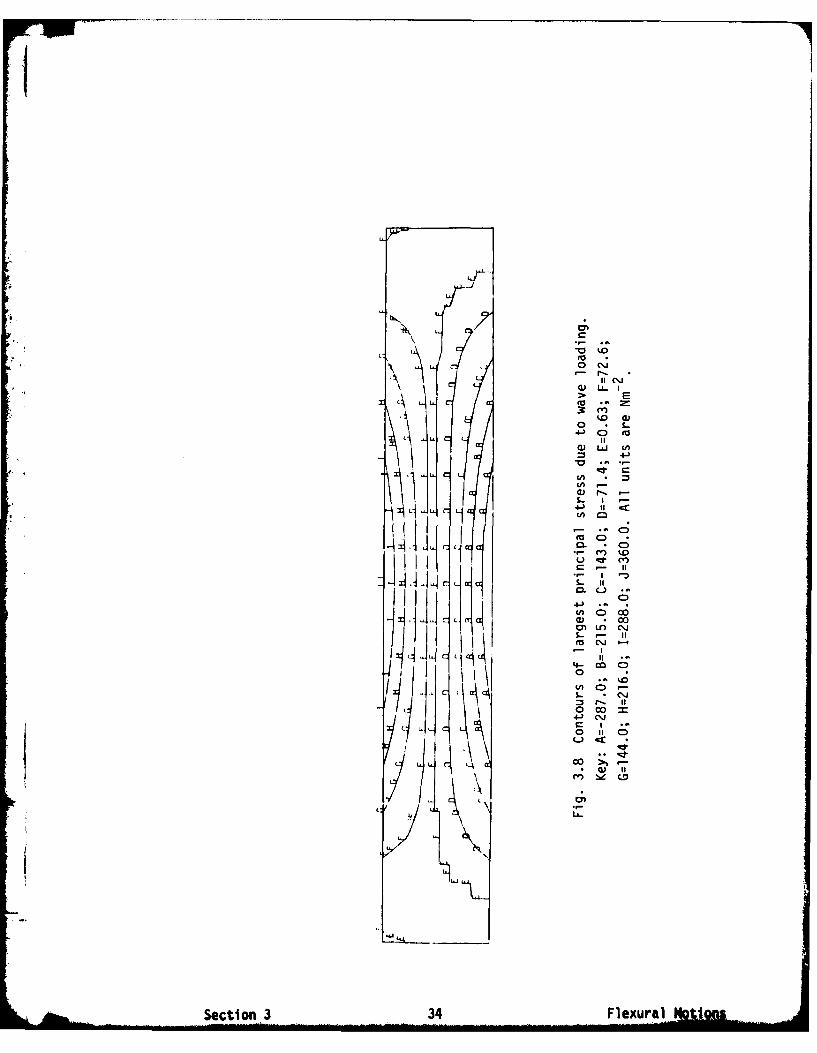
An alternative means of displaying the stress pattern is by means of a

contouring routine which draws lines of constant stress on the two-

dimensional cross-section (fig. 3.8). Here we see that so long as we do not

venture too close to the edges of the ice floe, the isopleths are parallel

to the upper and lower surfaces. Such a result would be expected in a thin

plate theory. The contouring routine shows clearly that the maximum

tensile stress is to be found at the central position on the floe's upper

surface, and the maximum compressive stress located directly beneath that

on the underside.

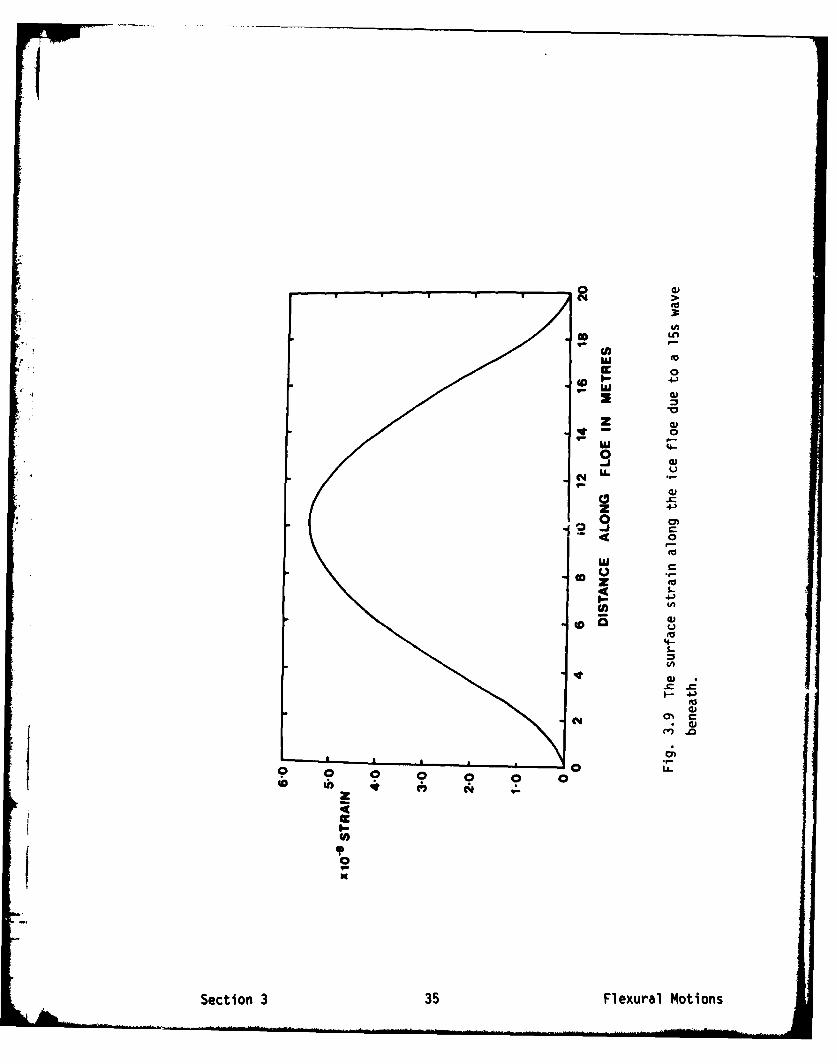
Bearing in mind that ultimately we wish to test our model with the Sea

Ice Group's strainmeters, we have converted the principal stresses to

principal strains by means of equations (3.1). This has been carried out

for all nodes along the floe's upper surface where the smaller principal

strain is several orders of magnitude smaller than the larger. The

directions of the axes of principal strain are such that the larger strain

is horizontal. Fig. 3.9 shows this strain along the ice floe. From this

graph we may say that the maximum strain experienced by a 20m by 3m floe

due to a 15s wave of Im amplitude is 5.5x10 -8 and that this value occurs

near the floe's centre. As an aside we may use this value to determine

* whether or not such a wave could fracture the floe and if not, what

amplitude would be necessary to break it. With an empirical fracture

strain of 3.0x10 - 5 (Goodman et al, 1980) we see that fracture Is unlikely

to occur.

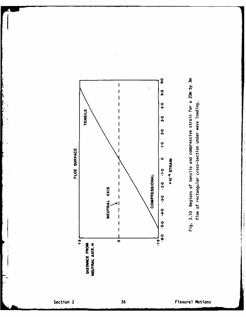
The change in strain through the floe is shown in fig. 3.10. As one

would expect for an Isotropic material, the strain vanishes mid-way

through (i.e. on the neutral axis), and the largest absolute principal


C"C

>I EX~ .-

'0

0-) LCJ to

CC

CU

C: ( IZI C

*~ 7) U

I ~ 0() C

L.If4-- M

0

O'n f ( NJ- IIj

-I

I

Section~~~4 3 4FeurlNto

II

' 'w

w 4

8.. U

9z

0

w

U) A400

II-

39W


Ii

(a~

Z to

IA COL C

,I o L"w I04 U 4J~

0A U

a K0Cl) cc I

w_ ,0 0n U

W -

-"I (A c

U. LA0

Section 3 36 Flexural M~otions

IL " - ....... ...... ... ..... . . .. ... ... .... .... .. ... . .. .. .. ..I. .. . .... .

strain at the surface is equal in magnitude but opposite in action to the

equivalent under-ice strain.

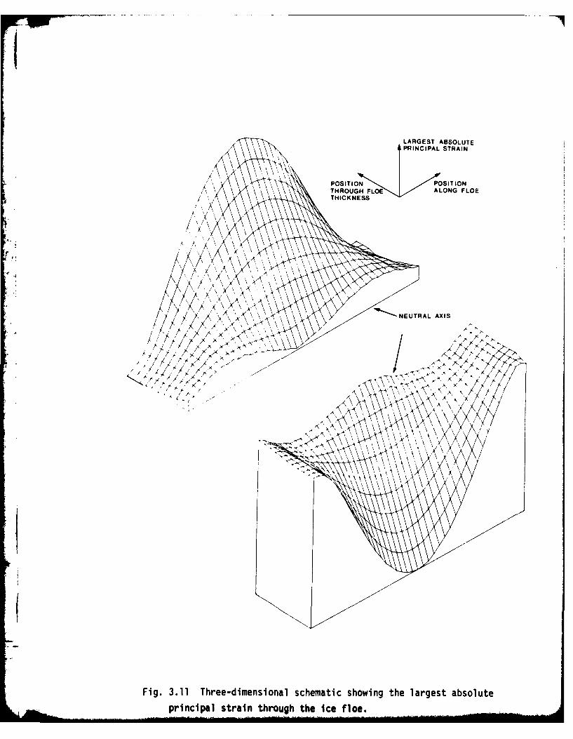
A novel way to view the strain field is shown in fig. 3.11 where the

tensile and compressive principal strains have been plotted as surfaces.

The neutral axis is clearly marked on each three-dimensional

representation. The plots should be Interpreted with reference to fig. 3.7

where the orientation of the principal axes may be seen in the angular

variation of the stress vectors (for a isotropic material in plane strain,

the prIncipal axes of stress and strain are alIgned).

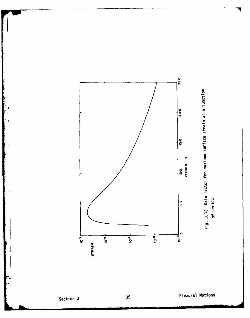
The final figure of this subsection, fIg. 3.12, shows how an ice floe of

twenty metre beam and three metre thickness will behave as ocean waves of

various periods pass beneath. The curve plotted is normal ised relative to

an incident wave amplitude of Im so that this should not be regarded as

the floe's response to a spectrum of waves, but rather as the magnitlude of

the frequency response function or gain factor (Bendat and Plersol, 1971)

of time series analysis. The curve represents surface strain as measured

by an imaginary Instrument located at the centre of the ice floe. As one

might expect, the strain at different wave periods is by no means constant.

For very long waves the radius of curvature of the wave is large so that

the floe bends only by a small amount leading to small surface strains. For

short waves, the radius of curvature is small and in principle one mIght

expect very large strains. This is not the case however, since both the

magnitude and the gradient of the pressure along the bottom of the floe

decrease rapidly as the period becomes very short. There is an optimum

period which will produce maximum strain and therefore maximum likelihood

of fracture. For the present floe this period is about 4s which is close to

the period at which resonance occurs for heave, sway and roll. This does

not necessarily mean that If energy of that period Is available in the

spectrum It will fracture the ice floe; rather we are saying that If the

spectrum were such that all frequencies were represented by equal amounts

of energy and that energy was sufficIent to break the floe, then waves of

period 4s would be the most likely to do so.

SectIon 3 37 Flexural

I7LARGEST ABSOLUTEPRINCIPAL STRAIN

A'POSITION POSIT IONTHROUGH FLOE ALONG FLOE

/ THICKNESS

A~''---NEUTRAL AXIS

A A

Fig. 3.1 The-dmnsoa sceai hwn helretasltprnia stai thog the ic le

9

i4-

N0

0

U

'4-

00

" Su l 0 n

04)

4-

0I-i

C0 0

t;

U-

'4-


3.5 Dynami: Analysis

The limitations of a static theory are not nearly so bad as one might

first suppose. So long as the pressure loading does not tune to the floe's

natural frequencies, the computed displacements and strains are reasonable

and are believed to accurately model the flexure. However, static analysis

tells us* nothing about those natural frequencies so that resonance in

flexure, which could foreseeably lead to the floe's ultimate destruction,

is glossed over. Ideally, one would like to be able to compute the cyclic

strains Induced as the wave propagated beneath, look at those strains with

passing time, possibly allowing the ice to deteriorate with time by some

sort of fatigue mechanism, and then at the end of the simulation say

something about the floe's survival. The problem is of course that such an

analysis is prohibitably expensive and even if run, the results would be

questionable due to the uncertainty of the physical properties of sea ice.

For these reasons the author has not attempted such a mammoth task as

implementing the necessary programs. The resonance problem still remains

however, and it is important to be able to discuss the natural frequencies

If one is to fully Interpret the static analysis.

We first pose the question: what is the fundamental frequency of

flexural oscillation and what are the frequencies of the first few

harmonics for an 20m by 3m ice floe floating in calm water? We will refer

to these frequencies as modes of oscillation. With no restraints applied

there will exist three rigid body modes (for a two-dimensional section)

which correspond to heave, sway and roll. In the present discussion we

suppose these modes to be Irrelevant and will consider the first mode of

Interest to be the primary flexural mode. We shall also limit our study to

bending or flexural modes since more esoteric oscillations, such as

tensional/compresslonal vibrations which might be Induced by an explosion

within the ice, are unlikely to be excited by ocean waves.

The determination of the natural frequencies of a body can be

simplified so that it is equivalent mathematically to a symmetric real

eIgenvalue problem. For a finite element mesh which reasonably represents

the body, one would expect a large number of nodes to be present. Each node

is permitted, for a two-dimensional section, to move In two orthogonal

Section 3 40 F Iexural Notions

I

directions known as degrees of freedom. It is clear that even though the

problem can be reduced to a symmetrIc eigenvalue problem, we are likely to

need a very large number of degrees of freedom to produce accurate results

so that our matrices are huge. This would lead to unacceptably long CPU

times and worse, to rounding errors.

Fortunately, many of the degrees of freedom in a large elgenvalue

problem have little effect on the eIgenvalues themselves. We may therefore

simplify our analysis further by reducing the problem to finding the

natural frequencies of an equivalent structure with less, but carefully

selected, degrees of freedom. The selection of the remaining "master

freedoms" is by no means simple and will not be discussed here; PAFEC

includes a facility to do this.

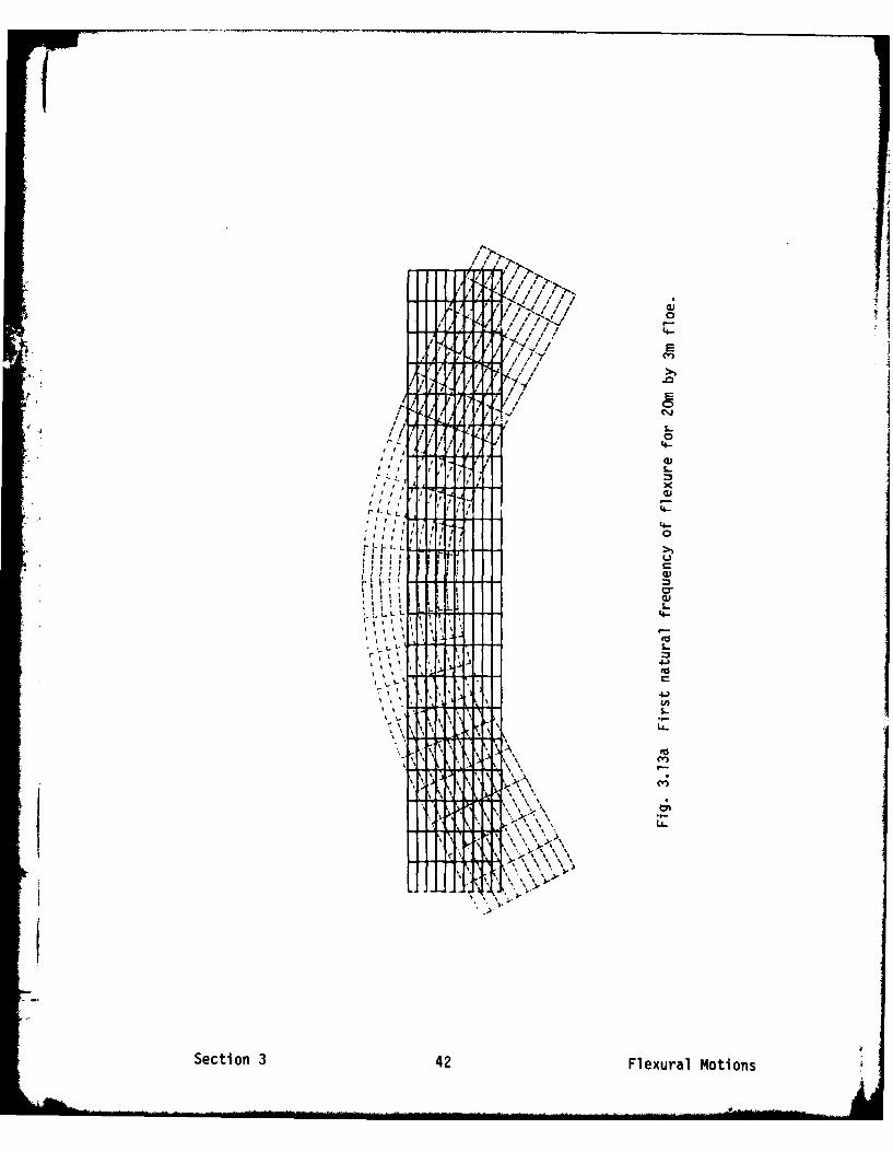
A modal analysis of our ice floe was carried out so as to compute its

natural frequencies. The first few modes are listed below:

MOOE FREQUENCY, HZ

1 19.13270 + 0.00013

2 47.28252 + 0.00002

3 82.75792 + 0.00001

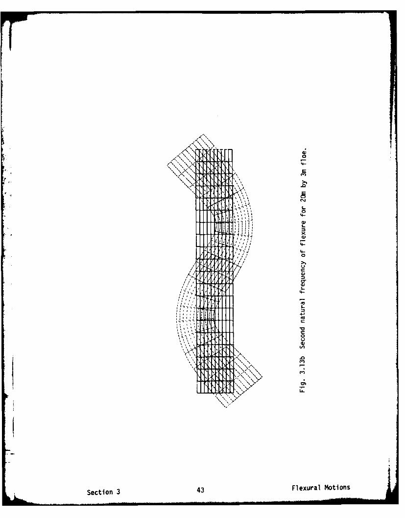
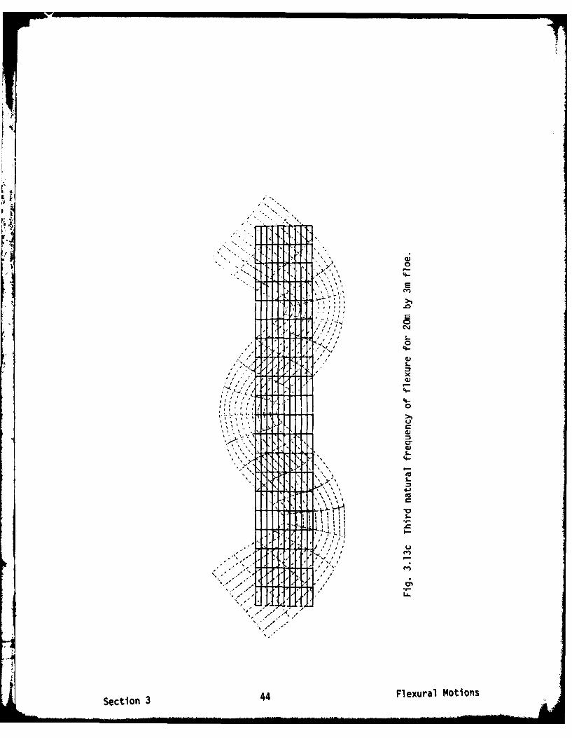
These modes correspond to fig. 3.13a,b and c respectively. The error bounds

are approximate but have all been calculated so as to include the

numerical error. It must be emphasised that these errors are an estimate

of numerical accuracy. They do not in any way bound the absolute error

caused by the approximations involved in using a finite element

representation of the "real" ice floe.

Since the natural frequencies of any structure form an orthogonal set,

any general distortion of the body may be regarded as the Infinite sum of

the modal distortions (for a system with an infinite number of degrees of

freedom). In any real analysis this summation may be discontinued aftsr

the first few modes since the series converges rapidly. Our iCe floe is no

execption and we will retain only the first few frequencies in subsequent


I'7

-I I I i I r

/ // ,>i

, "I

I I >.

, # I

SI I

I I /.

i ,.!,-

i" 111 I

* III

LL

* I (I)

* .L!

-[

I , L,,i.. ..

• ,, ,

=I

.IiScto 4 Flxua M tin

4 XX • 5X

-s s *-s44..,, , , , 5 5,_ -

SIXi

/ ,"' S

i iI S

I I , 5 3

i i, Il ,i II 44..

4...

,. d,,/a, t , =

ii /

Section 3 4 Flxra otos i

w

4 .' . ,, ,*

. . #, _

'o....

S - *

as.,' a 5~-o.

* a ' ,,-)

I I I*e

... .. . 5 ,4 - 0. n --€], , ,

,. .' ,.5.. , ,' , ,.

C. / • . o4

* , ,*" ,a 0 •

"

Sectin 3 4 Flexral Ht'on

TII ii1111 ~*a1..... a ~

calculations [1]. We are now in a position to reconsider the wave loading

and to determine the dynamic response due to waves passing beneath. If any

of the wave periods encountered were close to a mode, resonance would

occur, but in any realistic situation frictional forces within the

material would damp the resonance sufficiently to prevent infinitely

large strains. However, the resonant stresses produced might well be large

enough to permantently weaken the ice floes and to ultimately cause it to

break up. A secondary effect of the damping is to shift the body's natural

freqencies so that the Incident waves could foreseeably tune to modes at

lower frequencies. This shift is second order however, and for small

damping ratios is negl igibIe. The most convenient way to Impose damping on

the system of equations is to allow the material's physical properties to

become complex quantities. For the 20m by 3m ice floe, the modes occur at

frequencies which are well outside the significant energy regions of

typical open ocean spectra, so that resonance is unlikely. For this reason

damping is really only necessary for calculations where broad bandwidth

spectral observations are applied. In this case there is a possibility

that a minute amount of high frequency energy present in a spectrum might

lead to an unrealistic resonance.

As the size of the floe Increases, so the natural frequencies decrease

though the modal shapes remain the same. For an iceberg, there is a

distinct possibility that the frequencies will shift sufficiently to be

within the bandwidth of the wavj energy of the sea. The tanker Pine Ridge

broke in two in the Western Atlantic during December 1960 due to resonant

stresses set up during a storm, so Icebergs of similar and larger

dimensions might well break-up by the same mechanism. When the natural

frequencies of flexure are computed for a typical Antarctic Iceberg it is

found that the first flexural mode could easily be encouraged to resonate

by the available ocean wave energy. Ms. Monica Kristensen, a research

student at SPRI under the author's supervision, is currently considering

this mechanism in the interpretation of Iceberg data obtained during a

recent Antarctic cruise aboard HMS Endurance. Her work will be published

[1] The number of master degrees of freedom chosen for the dynamicsolution is finite so that we have already approximated the sum tosome extent.


In due course. In conclusion then, the author agrees with the original

suggestions by Goodman et al (1980) that resonant stressing due to waves

is a significant factor if not the predominant mechanism in the ultimate

destruction of Icebergs.

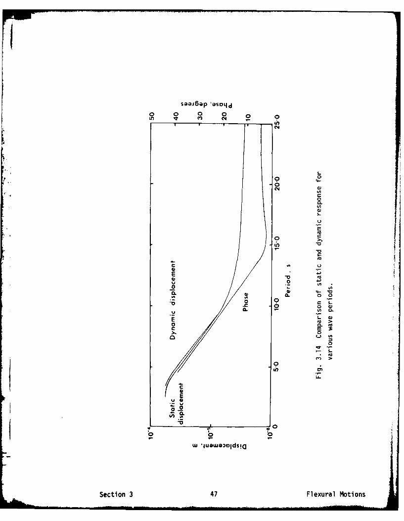
Returning to our discussion of sea ice we emphasise that resonantstressing Is unlikely to occur with any real ocean loading since the

dimensions of typical ice floes are too small. In fig. 3.14 the vertical

displacement and phase response of some arbitrary point within a 20m by 3m

ice floe are plotted alongside the equivalent static response at various

wave loading frequencies. The curves plotted have been normal ised so that

they are with respect to incident waves of unit amplitude. The small

difference between the static and dynamic results is most probably due to

rounding error, and contamination by the rigid body modes in the dynamic

solution. These errors will increase as the wave period decreases. Even so,

the reader will see that the curves agree well and that no resonance is

occurring within the bandwidth of energy considered. This confirms that

the destruction of ice floes by resonant stressing is unrealistic, and

further demonstrates that our static model is adequate for stress or

strain calculations. If the phase change between the loading and the

resulting flexural displacement is required then a dynamic model is

necessary since it Is clear from fig. 3.14 that the phase depends

critically on wave period.


saaj6aP 8OsDI.d

o0 0 0 0

o 06 4-

0CL

U

E

0

-C -U0 a

(a

U 4A

00

CE

00

to 0-

0 ~ 0 bLw 4seodi


4. PRELIMINARY COMPARISON OF THEORY WITH EAST GREENLAND DATA

4.1 Introduction

The previous sections have enabled us to compute theoretically all the

parameters that have been measured in a series of wave experiments carried

out by SPRI on sea ice in the Arctic. These resu Its are reported or will be

published elsewhere In great detail. See for example Squire and

Moore (1980), Squire and Martin (1980), Goodman et al (1980), and Moore

and Wadhams (1981). However, it was felt that no theoretical model could

really be presented without some experimental verification.

The 1979 field programme in east Greenland had two principal aims:

a) to quantify the motions of a single ice floe in waves; and b) to measure

the attenuation of waves through pack ice in the fjord and to relate this

to ice morphology. Several projects of type (a) were carried out and the

author has chosen one of these experiments to test the proposed model. The

comparisons are by no means exhaustive since suitable instrumentation to

measure roll, pitch and yaw was not available during the field trip, and

only a small subset of the recorded data is considered. Furthermore, the

only data available for comparison at this time is not ideally suited as a

test of the proposed model. The experiment we will discuss took place

on 14 September over the entire day. Three accelerometers were used to

measure heave, surge and sway, several strainmeters were used to measure

the floe's surface strain field in various locations and directions, and

the sea state was continuously monitored by means of a spar-loaded wave

buoy. Since the field trip the accelerometer data have been analysed as

random time series and have been integrated to give power spectra over

half-hour segments throughout the day. By considering the spectrum of each

of the floe-mounted Instruments with that produced from the simultaneous

wave buoy record, frequency response functions and coherences have also

been produced which have enabled us to treat the motions of the ice floe

Section 4 48 Preliminary Comparison

Independently from the Incident wave forcing.

4.2 Results of Comparison

The Ice floe upon which our experiments of 14 September took place was

by no means ideal. The floe was approximately 80m to 90m across and

between 3m and 4m thick. A im to 2m ridge adjacent to a refrozen meltpool

ran along one side of the floe and cut off a small flat apron from our

field of view. The instruments were deployed on a large area of suitably

flat ice as far as possible from this ridge. For the purpose of thenumerical simuiation several possible floe geometries were coded and

their effects on the resulting motions was studied in detail. For a floe of

., this size, it was found that an increase in diameter from 80m to 90m or a

change in thickness from 3m to 4m, had little effect on the resulting

motions. The ridge, however, did appear to influence the motions

significantly, though in all cases the theoretical curves fitted the data

better when a ridge and its corresponding keel were included in the

geometry.

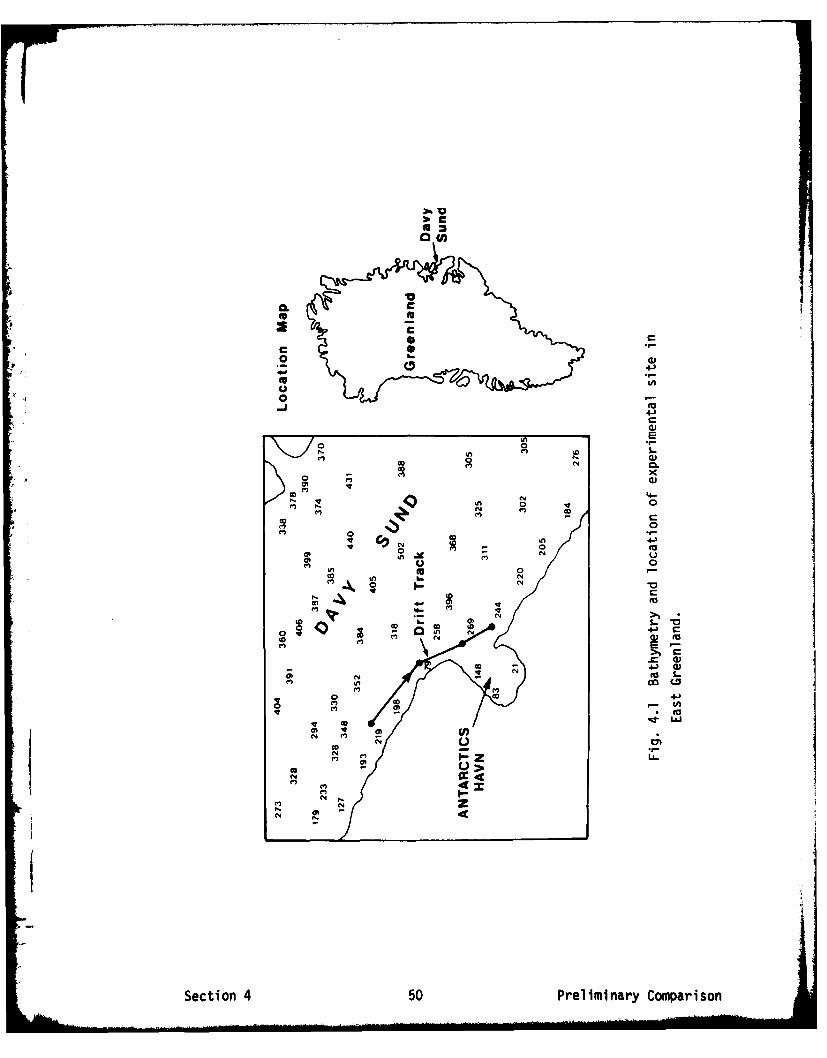
First attempts at a comparison between theory and experiment produced

unsatisfactory results. There were clear discrepancies for both sway and

strain, though the heave results looked promising. This can easily be

explained when the location and drift of the ice floe are considered in

relation to the shape and bathymetry of the fjord (fig. 4.1). Throughout

the experiment the floe drifted seawards in deep water at about 1.7 km/hr,

and always remained within a few hundred metres of a steep cliff face.

Waves entering the fjord from the open ocean would experience two effects;

firstly their spectrum would be distorted due to refraction, and secondly

waves would reflect from the cliffs alongside the ice floe. Neglecting

refraction, we are left with the considerable Influence that an almost

perfectly reflecting cliff could have on the motions of ice floes in Its

vicinity. For the sake of this argument we shall assume that the cliff Is a

perfect reflector for all the wave periods present In the fjord.

Consider a wavebuoy located in the fjord alongside the ice floe

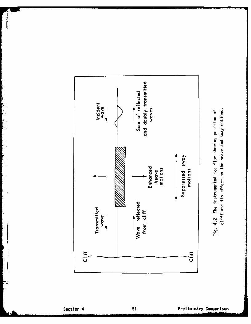
(fig. 4.2). This buoy will measure the superposition of both the Incident


2. €

'(A

C

C 1

0

4-)

O -

0

aJ

I,--

0 0

S0 N P a

0 0 .( Go NN~N

M A. 000

40 40 I

0 (1)OE C-'

(.7 UG0

W) - WCOC .13

aD)

V 01

CIDJCI M


-r-

U CA

110- b.0

>~q>

0 0-SM

0-> -0

0 In

- a

E 0U

0 >

Seci- 4 51 Prliinr Com0rion00AkA-

waves and the waves reflected back from the cliff face. When waves from any

direction are considered, the sea sampled by the buoy becomes very complex.

This is equally true when the motions of the floe Itself are considered. If

we consider the motions of heave, sway and strain In turn, we soon see that

a comparison of the data with the numerical model is not possible except

for the case of heave.

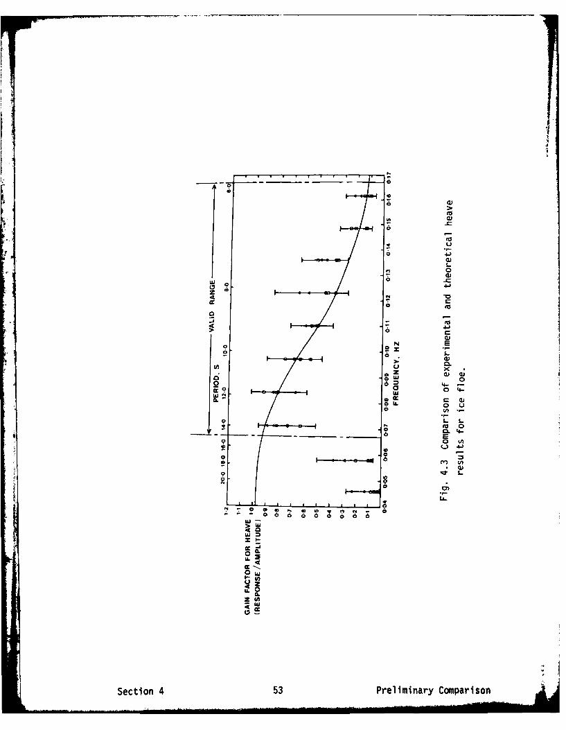
For heave, the two vertical accelerometers are used in the same sense,

so that although the floe is behaving in a very complex fashion due to the

Incident waves, the normal isatlon carried out during the data processing

Is sufficient to enable a reasonable test of the model to be made. The

heave data from five half-hour records are presented as a single frequency

response function in fig. 4.3, where each experiment is distinguished by a

different symbol. Confidence limits at the 95% level are also shown. The

valid range (6s to 15s) marked in the figure represents the range of

energy over which the original power spectra used to generate each plot

had significant energy. Outside this range the gain factors have no

physical meaning and are subject to large rounding error. Frequency

smoothing across fifteen contiguous energy values has been used to

generate each point. The smooth curve plotted on the data represents the

gain factor predicted by theory. There appears to be excellent agreement

between the model and experiment over the valid 6s to 15s range of

periods. When a significant keel is included in the geometry of the

numerical model, the theoretical curve changes little for low frequencies,

but as we move toward higher frequencies so the curve moves up

fractionally so as to centralize Itself within the confidence limits.

The sway and surge data pose much more serious problems since the jnormalisation is no longer reasonable if the wavebuoy record is

contaminated with wave energy reflected from the cliff face. Furthermore,

if we think In terms of normal Incidence for a moment, and suppose that the

sea close to the floe is made up of waves propagating in two opposing

directions, then the floe's sway motion wIll be considerably reduced. Thus

the frequency response functions created by normalisation of the sway and

surge records with respect to those of the wavebuoy will be very different

from those computed for an open water situation. Unfortunately, it is very

neary impossible to adjust either theory or observation, so that the sway


!U

ooS w

6 :)

0 ->

U. 0,,

- 4- )

0o0 6

00

o a. L

S

004-

I a J I I t t * )OIL0 4-

Section 4 53 Preliminary Comparisonmm i

and surge results can only be discussed In a qualItative sense.

The gain factors of the frequency response functions for the combined

horizontal motions show the same general shape as the theoretical curves

with a resonance between 8s and 1Os. However, the gain magnitudes are

considerably smaller than the theory predicts as would be expected from

the foregoing discussion. A detailed comparison must therefore await the

processing of further east Greenland data recorded on floes which were

further off the coast.

The strain data must also be subject to the same contamination due to

waves reflected from the cliffs. As before, the ice floe %,I1I experience a

wave load made up of both standing and travel I Ing waves of a magnitude

which depends on the wave's period. The reflection/transmission

characteristics of the floe will determine its subsequent flexural

behaviour. One would expect long waves to have small reflection

coefficients so that most of the wave energy will reach the cliffs and be

reflected back, whereas short waves would be considerably reduced in

amplitude at the Initial reflection from the floe's front edge. This leads

one to tentatively suggest that short waves might be less sensitive to

reflections from the cliffs, so that the theory would provide a better fit.

This is indeed the case with theory and data being in good agreement for

wave periods less than ten seconds, but becoming unacceptable as the wave

period is Increased.

At this stage then the author can present no better than an explanation

why the data and model produce different results. Until more data are

processed to produce the necessary frequency response functions for floes

which are a reasonable distance from the edge of the fjord, no detailed

theory can model the ice floe's motions. This analysis promises to take at

least two months from the date of publication of this article due to the

complex problems which arise when strainmeter data are processed. A later

paper to be published In the literature will provide a more convincing

verification of the proposed numerical model.


5. 81BL I OGRAPHY

Bendat, J.S., and A.G. Piersol. 1971. Random Data: Analysis and Measurement

Procedures, Wi ley-I nterscIence, New York, 407pp.

Desal, C.S., and J.F. Abel. 1972. Introduction to the Finite Element Method.

Van Nostrand Reinhold Co., 477pp.

SFrank, W. 1967. Oscillation of cylinders in or below the free surface of

deep fluids. NSRDC Rep. 2375, Naval Ship Research and Development

Center, Washington D.C., U.S., 40pp.

Goodman, D.J., Wadhams, P., and V.A. Squire. 1980. The flexural response of a

tabular ice island to ocean swell. Annals of Glaciology, 1, 23-27.

Hendrickson, J.A. 1966. Interaction theory for a floating elastic sheet of

finite length with gravity waves In water of finite depth.

Rep. NBy-62185 by Natn. Engng. Science Co., Pasadena, Calif. for U.S.

Naval Engng. Lab., Port Hueneme, Cal I f., 178pp.

Jaeger, J.C. 1956. Elasticity, Fracture and flow with Engineering and

Geological Applications. Methuen and Co., Ltd., New York, 152pp.

John, F. 1950. On the motion of floating bodies II, Comm. Pure. ADp.

Math., 3, 45-101.

Lamb, H. 1962. Hydrodynamics, Cambridge University Press, 6th ed., 738pp.

Lee, C.M. 1976. Motion characteristics of floating bodies. J _

Res., 20(4), 181-189.

McCorm ick, M.E. 1973. Ocean Eng I neer i ng Wave Mechan i cs, W I I ey- I ntersc i ence,

John Wi ley and Sons, Lond., 179pp.

Moore, S.C., and P. Wadhams. 1981. Recent developments in stralnmeter design.

Proceedings of the Workshop on Sea Ice Field Measurement, St. Johns,

Newfoundland, April 29-May 1, 1980, 99-125.

Section 5 .5

Robin, G.de Q. 1963. Wave propagation through fields of pack ice. Phil.

Trans. R. Soc. A, 255(1057), 313-339.

Squire, V.A. 1978. Dynamics of Ocean Waves in a Continuous Sea Ice Cover,

Ph.D. dissertation, Univ. of Cambridge, England, 191pp.

Squire, V.A., and S. Martin. 1980. A field study of the physical properites,

response to swell, and subsequent fracture of a single Ice floe In the

winter Bering Sea. ScIentific Rep. 18, Dept. of Atmospheric Sciences and

Oceanography, Univ. of Washington, U.S. 56pp.

Squire, V.A., and S.C. Moore. 1980. Direct measurement of the attenuation of

ocean waves by pack ice. Nature Lond., 283(5745), 365-368.

Timoshenko, S., and S. Woinowsy-Krieger. 1959. Theory of Plates and Shells,

McGraw-Hi II Book Co., New York, 2nd ed., 580pp.

Timoshenko, S., Young, D.H., and W. Weaver Jr. 1974. Vibrational Problems in

Engineering, John Wiley and Sons, New York, 4th ed., 521pp.

Ursell, F. 1949a. On the heaving motion of a circular cylinder on the

surface of a fluid. Q. JI. Mech. appl. Math., 2, 218-231.

Ursell, F. 1949b. On the roiling motion of cylinders in the surface of a

fluid. Q. JI. Mech. appl. Math., 2, 335-353.

Vugts, J.H. 19 68a. The hydrodynamic coefficients for swaying, heaving and

rolling cylinders in a free surface. Rep. No. 112S, Nederlands

Scheepsstudiecentrum Tno, Leeghwaterstraat 5, Delft, Netherlands, 31pp.

Vugts, J.H. 1968b. Cylinder motions in beam waves. Rep. No. 115S, Nederlands

Scheepsstudlecentrum Tno, Leeghwaterstraat 5, Delft, Netherlands, 23pp.

Wadhams, P. 1973a. Attenuation of swell by sea Ice. J. Geophys.

Res., 78(18), 3552-3563.

Wadhams, P. 1973b. The Effect of a Sea Ice Cover on Ocean Surface Waves,

Ph.D. dissertation, Univ. of Cambridge, England, 223pp.

5.. 56 Wil

Wadhams, P. 1978. Wave decay in the marginal ice zone measured from a

submarine. Deep Sea Res., 25, 23-40.

-Wehausen, J.V. 1971. The motion of floating bodies. Annual Review of Fluid

Mechanics, 3, 237-268.

Wehausen, J.V., and E.V. Laitone. 1960. Surface Waves. Encyclopeia of Physics,

Vol. IX, Springer-Verlag, Berlin, 446-778.

Zienkiewicz, O.C. 1977. The Finite Element Method, McGraw-Hill Book

Co. (UK) Ltd., 3rd ed., 787pp.

'S

seto 7Bbigah

Documents

IIIIIIIImIuuuuu mhhhhhmhhhhulllllllllmllll flflflflflflfllllll · Although no detailed comparison with recorded wave data can be carried ... Finally I thank Dougal Goodman and