7 AD-A107 667 WEIDLIN6ER ASSOCIATES MENLO PARK CA F/6 8/11SITE-DEPENDENT GROUND MOTIONS FROM DISTANT EARTHQUAKES. REVISED-ETC(U)DEC 8S G L WOJCIK., J ISENBERG, W S DUNBAR F49620-80-C-0OG9

UNCLASSIFIED R-8065 AFOSR-YR-81-0723 N12 F21lfff fl ffiifLoisfl.fnfiIIIIIIIIIIIIIuEEEIIEEIIEEEIEIIIIIEEIIIIEEEEIhlllEEEEEEE

WEIDLINGER ASSOCIATES

3MW SAND HILL ROADBUILDING 4, SUITE 245

MENLO PARK, CALIFORNIA 942

SITE-DEPENDENT GROUND MOTIONSFROM DISTANT EARTHQUAKES

By

G.L. WojcikJ. Isenberg o

W.S. Dunbar

Prepared for

Air Force Office of Scientific Research

Boling AFB, Washington, D.C. 20332

and

Air Force Geophysics LaboratoryTerrestrial Sciences Division

Hanscom AFB, Massachusetts 01731

Final ReportAFOSR Contract F4962040-C49

For the Period 1 October 1979 to 31 December 1980

9Approved for public release;

distributionl unlimited*

~UNCLASSIFIED

SECURITY CLASSIFICATION OF THIS PAG .ten Dg-'ntered)

READ INSTRUCTIONSREPORT BEFORE COMPLETING FORM

,1a. GOVT ACCESSION NO .2-RECIPIENT'S CATALOG NUMBER'AFOSR./7 - -0 7 2 3 1)GVW./.,o.Z 7. _____,_._.

4. TITLE[ (and Svb I)IJ J. Type ai RE.PORT S tP-ll"06 ev --

Site-Dependent Ground Motions Final Report-from Distant Earthquakes- / 1 Oct 1979 T--31 Dec 1980U7-Pe"UWNr aimG. RE[POR T NUMBER"

R 8065

7. 1HT ..O . .... . CONTRACT OR GRANT NUMUER(d)!G. L. Wojcik

J. Isenberg F49620-80-C-0009W. S. Dunbar

9 PRFiIr6WIMG ORGANIZATION NAME AND ADDRESS 10. PROGRAM ELEMENT. PROJECT. TASKWeidlinger Associates AREA, WoRK UNIT NUMUERS3000 Sand Hill Road, Building 4, Suite 245Menlo Park, California 94025 O. 36 ? (R

II. CONTROLLING OFFICE NAME AND ADDRESS -- 1.IRIPORT OATE I

Air Force Office of Scientific Research " /-(--- / 9 L2

Bldg. 410, Bolling AFB, Washington, DC 20332 109 OFPAGES109 /;

14. MONITORING AGENCY NAME AOORRESS(OI diffIrswe fIom CandIffInd Office) I. SECURITY CLASS. (of this repoFT

UNCLASSIFIED

1I. DECLASSIFICATION/OOINGRADINGSCHEDULE

16. OISTRIBUTION STATEMENT (of OAo Ro€pet)

Ipp,'oved for public roloaSS:dietribution unlimited.

17. DISTRIBUTION STATEMENT (of I%. abtoct entered In Btck t0 II dllerent tram Reprt)

IS. SUPPLIEMENTARY NOTES

IS11 KEY WIORDOS (Conehbwo on revee side It necoeary and Identify, by block number) "Geology Basin Resonance Minuteman Wing V

I Seismology Body Waves 7

Denver Basin Seismic Alarms

20. ABSTRACT (Confihue an revwee side If necooowm and Identify 7 bloek mmb.)

This study examines geological and seismological reasons for patterns ofguidance alarms in Minuteman Wing V due to the 1975 Pocatello Valley, Idahoand 1979 St. Elias, Alaska earthquakes. Two features are identified w'hichtogether could cause these patterns of alarms. First is the existence oflightly-damped missile suspension system modes in the period window from2 to 6 seconds. Second is a 2 to 3 km sedimentary layer underlying the wing,with natural frequencies in this critical period window. Near-vertically- J

DO F'A 7S 1473 EoIIoNoP 'NOV ssoBSOLETE UNCLASSIFIEDSECURITY CLASSIFICATION OF TI41S PAGE (Wmi Data Emefd)

20. ABSTRACT (CONTINUED)

.--iincident P and S seismic body waves which propagate directly from thesource through the crust and upper mantle can interact with this structure.A Haskell-Thomson program for body wave propagation in a layered model indi-cates that peak ground shaking can vary by a factor of 2 at adjacent Wing Vflights. Differences are due to variations in sediment thicknesses andwavespeeds, deduced from oil well log and laboratory data. Therefore, Wing Valarm'-patterns appear to be caused by the coincidence of three factors:1) high gain of the 2 to 6 second suspension system modes; 2) incident bodywaves in this period range; and 3) sedimentary column resonance periods closeto the suspension system natural periods. If the first two are sufficient totrigger alarms, then the third would cause anomalous patterns due to relative

amplification between flights. Escarpments, basin edges and similar featuresare not likely to cause the observed distribution of alarms because they pro-duce resonances at periods too short to affect the Missile GuidanCe Set. Thisis confirmed by a finite element analysis of the escarpment for vertically-incident body waves.

W,

P .-

--- aglow

WEIDLINGER ASSOCIATES-3000 SAND HILL ROADBUILDING 4, SUITE 245

MENLO PARK, CALIFORNIA 94025

SITE-DEPENDENT GROUND MOTIONSFROM DISTANT EARTHQUAKES

By

G.L. WojcikJ. Isenberg

W.S. Dunbar

Prepared for

Air Force Office of Scientific Researchboiling AFB, Washington, D.C. 20332

and

Air Force Geophysics LaboratoryTerrestrial Sciences Division

Hanscom AFB, Massachusetts 01731

Final ReportAFOSR Contract F4962040-C-0009

For the Period I 0ctihcr 1979 to 31 December 1910

lowk

V.I

C1 .*-. - *.

I

ABSTRACT

This study examines geologic and seismological reasons for patterns

of guidance alarms in Minuteman Wing V due to the 1975 Pocatello Valley,

Idaho and 1979 St. Elias, Alaska earthquakes. Two features are identified

which together could cause these patterns of alarms. First is the existence

of lightly-damped missile suspension system modes in the period window from

2 to 6 seconds. Second is a 2 to 3 km sedimentary layer underlying the wing,

with natural frequencies in this critical period window. Near-vertically-

incident P and S seismic body waves which propagate directly from the

source through the crust and upper mantle can interact with this structure.

A Haskell-Thomson program for body wave propagation in a layered model indi-

cates that peak ground shaking can vary by a factor of 2 at adjacent Wing V

flights. Differences are due to variations in sediment thicknesses and

wavespeeds, deduced from oil well log and laboratory data. Therefore, Wing V

alarm patterns appear to be caused by the coincidence of three factors:

1) high gain of the 2 to 6 second suspension system modes; 2) incident body

waves in this period range; and 3) sedimentary column resonance periods close

to the suspension system natural periods. If the first two are sufficient to

trigger alarms, then the third would cause anomalous patterns due to relative

amplification between flights. Escarpments, basin edges and similar features

are not likely to cause the observed distribution of alarms because they pro-

duce resonances at periods too short to affect the Missile Guidance Set. This

is confirmed by a finite element analysis of the escarpment for vertically-

incident body waves.

i;jj

ACKNOWLEDGMENTS

The research effort reported here benefited from infornation and com-

ments by a number of individuals. Dr. Ker Thomson of the Air Force Geo-

physics Laboratory instigated this research effort and provided preliminary

data. Prof. Robert B. Smith, Prof. Walter Arabasz and Mr. Kevin Kilty at

the University of Utah were consultants early in the effort and supplied pre-

liminary geophysical data on the Denver Basin area, particularly Tertiary

geology, oil well log data and Landsat imagery. Mr. Thomas S. Summers of

Eyring Research Institute, Inc. was a valuable and timely source of data

on Wing V seismic alarms from both the Pocatello Valley and St. Elias earth-

quakes. Mr. Robert Hume of TRW provided a useful discussion of unclassified

data pertaining to Wing V seismic discriminants. Messrs. Norman Lipner and

Gary Teraoka of TRW made available the Porter and O'Brien Wing V subsurface

site investigations and related data. Prof. Amos Nur and Ms. Carol

Tosaya of Stanford University supplied valuable data and discussion on rock

properties. Dr. David Boore of USGS, Menlo Park, California kindly read a

draft of Section 3. In addition, the technical assitance of Penny Sevison

for the illustrations, Edith Durfey for much of the geologic data reduction,

and Myrtle Carey and Pam Hagan for typing the report, is gratefully acknowledged.

2

TABLE OF CONTENTS

Section Page

1 INTRODUCTION ........... ...................... 9

1.1 Description of Wing V .... ............... .I... 111.2 Alarm Distribution and Early Hypotheses ... ...... 141.3 Source Modeling and Synthetic Seismograms ........ 20

2 GEOLOGICAL EVOLUTION OF THE WING V AREA .......... ... 23

2.1 Tectonic and Geologic Background .. ......... ... 232.2 The Denver Basin ..... ................. .... 29

3 GROUND MOTIONS FROM THE POCATELLO VALLEY AND ST. ELIASEVENTS ......... ......................... .... 39

3.1 The St. Elias Earthquake ... ............. ... 39

3.2 The Pocatello Valley Earthquake ............. ... 46

4 VELOCITY STRUCTURE IN THE DENVER BASIN ........... ... 53

4.1 P Wave Models ...... ................... .... 534.2 S Wave and Density Models ... ............. .... 59

5 SEISMIC RESONSE OF DENVER BASIN SEDIMENTS ....... ... 65

5.1 Sedimentary Column Resonance Calculations ........ 665.2 Additional Wave Propagation Mechanisms ...... ... 84

6 SUMMARY AND CONCLUSIONS .... ................ .... 87

7 REFERENCES ........ ....................... .... 92

8 APPENDIX A ........... ....................... A-l

A.1 Introduction ...... ................... .... A-1A.2 Numerical Method .................... A-1A.3 Application to Goshen Hole Escarpment. ....... .... A-2A.4 Conclusions and Suggestions for Extending

the Method ....... .................... ... A-3

APPENDIX REFERENCES ......... .................. A-13

3

r

LIST OF FIGURES

Figure Page

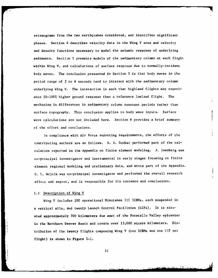
1-1 Distribution of Wing V flights (A through T) in the tri-state area of Wyoming, Nebraska and Colorado .... ........ 12

1-2 Resonance curves for longer period, lightly damped modesof suspension system .......... .................... 15

1-3 Amplitude versus number of cycles for longer period

suspension system modes ....... .................. ... 16

1-4 Distribution of seismic alarms caused by the 1975 PocatelloValley and 1979 St. Elias earthquakes .. ........... ... 17

1-5 Comparison of synthetic seismograms with and withoutuniform sediment over travel path ... ............. ... 22

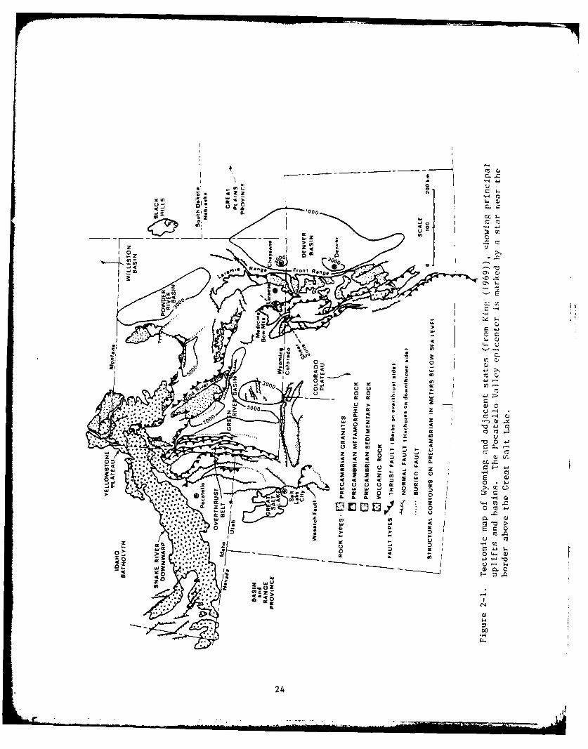
2-1 Tectonic map of Wyoming and adjacent states, showing

principal uplifts and basins ...... ................ ... 24

2-2 Sections illustrating structural evolution of the FrontRange of Colorado ....... ..................... .... 27

2-3 Sketches illustrating structural features found alonguplifts in the Central and Southern Rocky Mountains . . . . 28

2-4 Approximate structural contour map of pre-Mississippianrocks in the Denver Basin ...... ................. ... 30

2-5 Section AA' of Figure 2-4 illustrating formation thick-

nesses in the Denver Basin on a line bisecting Wing V . . . 33

2-6 Sections in Figure 2-4 illustrating Denver Basin structureon the Laramie Range east flank ..... .............. ... 34

2-7 Distribution of Tertiary and older surface rocks in thetri-state area ........ ....................... .... 35

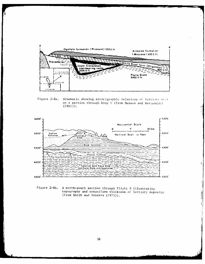
2-8a Schematic showing stratigraphic relations of Tertiaryrock on a section through Wing V ..... .............. ... 38

2-8b A north-south section through Flight B illustratingtopography and nonuniform thickness of Tertiary deposits. 38

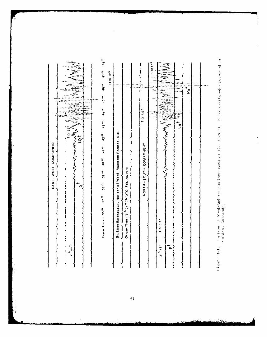
3-1 Horizontal Wood-Anderson seismograms of the 1979 St. Eliasearthquake recorded at Golden, Colorado .. .......... ... 41

3-2a Observed and theoretical dispersion of continentalRayleigh waves ........ ....................... .... 43

4

LIST OF FIGURES (CONTINUED)

Figure Page

3-2b Palisades NS seismogram of Lg and Rg waves from Yukonaftershock of March 1, 1955 ........ ................. 43

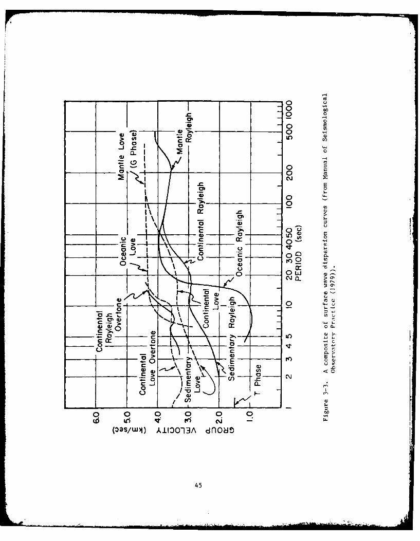
3-3 A composite of surface wave dispersion curves ........... ... 45

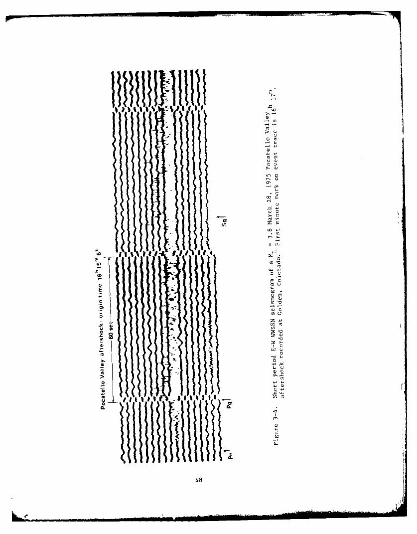
3-4 Short period E-W WWSSN seismogram of a ML = 3.8March 28, 1975 Pocatello Valley aftershock recorded atGolden, Colorado ......... ...................... ... 48

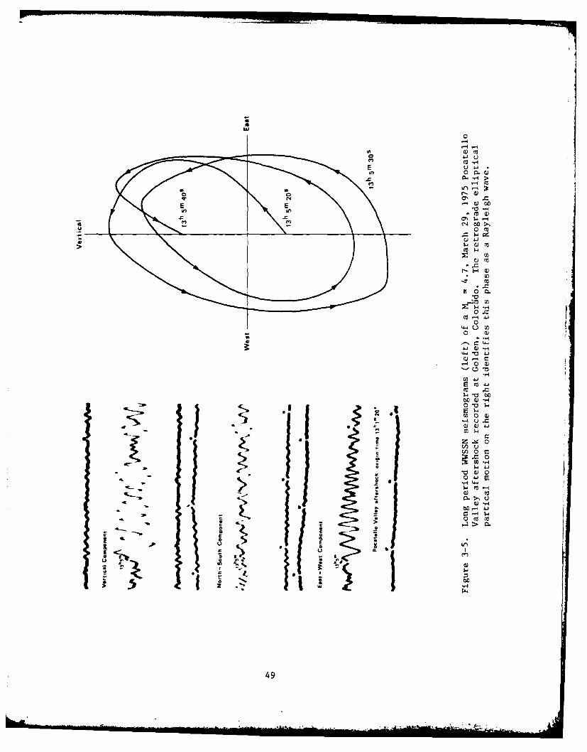
3-5 Long period WWSSN seismograms of a ML = 4.7 March 29, 1975Pocatello Valley aftershock recorded at Golden, Colorado.The retrograde elliptical partical motion on the rightidentifies this phase as a Rayleigh wave ... .......... ... 49

3-6 A cross-section through Wyoming aligned with the propagationpath from the Pocatello Valley epicenter to Wing V .. ..... 51

4-1 A - Velocity function from well logs within Flights S, Rand P. B - Faust's fit of velocity functions in the GoshenHole (Flight S) ........ ....................... .... 54

4-2 Distribution of fast, moderate and slow velocities in near

surface rock ......... ........................ ... 58

4-3 Laboratory data on Pierre Shale and other rock ......... ... 60

5-1 Examples of reflection surveys illustrating uniformityof deeper sediments near Flights Q and S in the DenverBasin; vertical travel times in seconds .............. .... 69

5-2 Velocity and density functions at Flights P and S ... ...... 72

5-3a Amplitude spectra for slow, nominal and fast velocitymodels with S wave input at normal incidence .......... ... 73

5-3b (same as above) ........ ....................... .... 73

5-3c (same as above) ........ ....................... .... 74

5-4a Amplitude spectra for slow, nominal and fast velocitymodels with P wave input at normal incidence .......... ... 74

5-4b (same as above) ........ ....................... .... 75

5-4c (same as above) ........ ....................... .... 75

5-5 Spectral. ratios for S wave input with nominal velocitymodels ............ .......................... ... 78

5

LIST OF FIGURES (CONCLUDED)

Figure Page

5-6 Spectral ratios for S wave input with a fast model atFlight S and slow modes at Flights P and H ........... .... 79

5-7a Spectral ratios >1.5 for 2.5< period< 3.5 seconds .. ..... 81

5-7b Spectral ratios >1.5 for 2.5<period< 3.5 seconds .. ..... 81

5-7c Spectral ratios >1.35 for 2.5<period< 3.5 seconds ........ 82

5-8 Spectral ratios >1.5 for 3< period< 3.5 seconds ...... ... 82

5-9 Spectral ratios >1.5 for 2< periods< 2.5 seconds ... ...... 83

5-10 Approximate sediment depths over Wing V .. .......... ... 83

A-i Finite element model of escarpment (Wing V highlands-lowlands seismic alarm anomaly) ..... .............. ... A-5

A-2 Application of Green's function approach to exampleof Wing V seismic alarm anomaly ........ .............. A-6

A-3 Ricker wavelet obtained by a superposition of finiteelement ramp responses for the highland soil column . . . . A-7

A-4 Vertical seismograms on lowland - P-wave input,5 Hz Ricker wavelet .......... .................... A-8

A-5 Vertical seismograms on highland - P-wave input,5 Hz Ricker wavelet .......... .................... A-9

A-6 Vertical seismograms of scattered waves on highland -

P-wave input ............ ........................ A-10

scattered spectrum

A-7 Power spectral density ratio incident spectrum

for a lowlands point with P-wave input (vertical) ..... ... A-Il

A-8 Power spectral density ratio scattered spectrum

incident spectrum

for a highlands point with P-wave input (vertical). . . . . A-12

6

I LIST OF TABLES

ITable Page

2-1 Geologic Time Scale .. .. .. ....... ........... 25

5-1 Average Formation Thicknesses Under Wing V Flights .. .. ... 68

7/8

SECTION 1

INTRODUCTION

In 1975 a magnitude 6.0 (ML) earthquake occurred in Pocatello Valley,

Idaho, near the southeast Idaho-Utah border (Arabasz, et al. (1980)). It was

located within the southern part of the Intermountain Seismic Belt (Smith

and Sbar (1974)) where the last local event of comparable magnitude took

place in 1962 (Cache Valley, Utah; ML = 5.7). In addition to causing

moderate damage in the epicentral region, the earthquake had a significant

effect 640 kilometers east of the epicenter at the 90th Strategic Missile

Wing, Wing V, near F. E. Warren Air Force Base, Cheyenne, Wyoming. Unex-

pected and unprecedented operational mode changes (seismic alarms) were trig-

gered in 42% of the missile force, distributed in a southeast swath across

the wing. The apparent cause was long period (2 to 6 second), low amplitude

ground shaking. The subject of this report is a quantitative investigation

of the phenomenon in terms of ICBM response and seismic response of the Wing V

area.

The investigation was begun as a computational effort to explain the

distribution of seismic alarms. Initial emphasis was on topography, parti-

cularly the apparent correlation of alarms with highland sites, which were

separated from lowland sites by the Goshen Hole escarpment (S 200 meter ele-

vation change). Preliminary studies were conducted using finite element regional

models together with seismic input derived from synthetic seismograms, Rodi

et al. (1979). It soon became apparent that no significant interaction be-

tween topography and seismic waves could occur in the period window of inter-

est, 2 to 6 seconds, so as to cause the observed alarm distribution. The syn-

thetic seismograms exhibited considerable surface wave motion which suggested

9

that the interaction of surface waves with local geology may have been a cause.

However, work by Hume (1980) showed that body wave arrivals were correlated

with more subtle Wing V seismic discriminants from distant earthquakes, leav-

ing the question of causative wave type unresolved.

In 1979, four years after the Pocatello Valley event, the St. Elias

earthquake in southeast Alaska triggered seismic alarms in 46% of the Wing V

missile force. A surface wave magnitude (Ms) of 7.1 was reported, Lahr (1980),

Boatwright (1980). The alarm distribution differed from the previous case, as diJ

the duration, phasing and amplitude of seismic waves. St. Elias seismograms

recorded at Golden, Colorado, in conjunction with alarm timing data collected

by Summers (1980) suggested that body waves were responsible for the St. Elias

seismic alarms. This is consistent with Hume's observations.

After reevaluating the Wing V problem, an effort was made to collect data

on Wing V system response, seismic inputs, local geology and tectonics, in order

to narrow the choice of possible causative mechanisms. It was necessary to

characterize three cypes of behavior: 1) response of the Minuteman ICBM, its

suspension system and the surrounding silo (structure response); 2) nature of

the seismic input (source and path effects); and 3) ground response due to the

interaction of seismic waves with local geology (site response). These are

basic features of any problem in engineering seismology. In the following

sections, these data are described and finally applied to a calculational model

in Section 5.

The present report consists of five sections. Section 1 introduces the

*problem and provides background data on the Wing V system and previous Air

Force sponsored work addressing local response within Wing V. Section 2 des-

cribes the geological evolution of the area in order to identify geologic and

structural features relevant to the problem. Section 3 presents available

10

. .... .... . . . . . I 1 . . . . .I

seismograms from the two earthquakes considered, and identifies significant

phases. Section 4 describes velocity data in the Wing V area and velocity

and density functions necessary to model the seismic response of underlying

sediments. Section 5 presents models of the sedimentary column at each flight

within Wing V, and calculations of surface response due to normally-incident

body waves. The conclusion presented in Section 5 is that body waves in the

period range of 2 to 6 seconds tend to interact with the sedimentary column

underlying Wing V. The interaction is such that highland flights may experi-

ence 50-100% higher ground response than a reference lowland flight. The

mechanism is differences in sedimentary column resonant periods rather than

surface topography. This conclusion applies to body wave inputs. Surface

wave calculations are not included here. Section 6 provides a brief summary

of the effort and conclusions.

In compliance with Air Force reporting requirements, the efforts of the

contributing authors are as follows. W. S. Dunbar performed part of the cal-

culation reported in the Appendix on finite element modeling. J. Isenberg was

co-principal investigator and instrumental in early stages focusing on finite

element regional modeling and preliminary data, and wrote part of the Appendix.

G. L. Wojcik was co-principal investigator and performed the overall research

effort and report, and is responsible for its contents and conclusions.

1.1 Description of Wing V

Wing V includes 200 operational Minuteman III ICBMs, each suspended in

a vertical silo, and twenty Launch Control Facilities (LCFs). It is situ-

ated approximately 700 kilometers due east of the Pocatello Valley epicenter

in the Northern Denver Basin and covers over 13,000 square kilometers. Dis-

tribution of the twenty flights composing Wing V (ten ICBMs and one ICF per

flight) is shown in Figure 1-1.

i11

..............................................

Cl)

100

.1c 0

~L. -- II. ~ -cc

41,a

AtI 0a

I AVU 3 .. CID ., -n

-4- C1'

r4 0

-I- 0. 0

_j 0 m

0

c -1

'4

D N

12

The 200 ICBMs can be viewed as an array of seismic instruments (inverted

pendulums) capable of registering ground motion. This is accomplished as a

secondary function by the Missile Guidance Set (MGS) which includes an iner-

tial platform, digital computer, gravity level, gyrocompass and gyro accelero-

meter. Resolution of the MGS is rather crude, however, in comparison to a con-

ventional seismic instrument. For example, the data sample interval is on the

order of minutes and disruption counts are recorded rather than motion levels.

The output of principal concern here is the so-called seismic alarm, an in-

struction (based on leveling counts) for the system to switch from a very

stable gravity leveling mode to a more robust gyroscopic leveling mode (PIGA

leveling). Therefore, the alarm is essentially a seismic switch indicating

that motion of the MGS has repeatedly exceeded some value. Details of the

alarm transfer function are presently being investigated by the Air Force

under a full-scale testing program. The available data on MGS response are

described below.

The Minuteman III silo mounted ICBMs in Wing V are each supported from

a base ring in a missile cage which is in turn suspended by an upgraded Boe-

ing Missile Suspension System within the silo. Boeing has represented the

overall response of the system to external seismic input by a linear model

with twelve coupled degrees of freedom. The coefficient matrices of the re-

* sulting linear system of ordinary differential equations are determined experi-

mentally by "plucking" the missile in its suspension system. This is in con-

trast to real seismic inputs corresponding to motion of the silo (ground mo-

tion) rather than missile motion. The linearity assumption guarantees that

the two approaches are equivalent. Actually, there is some suspicion that

at the low amplitudes and long periods of interest here, nonlinear system

* Iresponse is significant. This question will be clarified by the full-scale

testing program which mimics silo inputs rather than missile inputs.

13

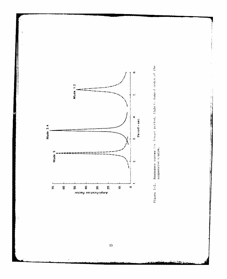
The classical linear approach yields theoretical uncoupled modes of

the system. The first five modes are long period (2-6 seconds) and lightly

damped (damping ratio less than or equal to .01). Resonance curves for these

modes are shown in Figure 1-2. The remaining seven modes have periods on the

order of one second or less and are more highly damped. It has been strongly

suggested that the longer period modes, specifically the 3.4 second mode,

are responsible for the seismic alarms. One basis is data from more

subtle MGS discriminants registering distant earthquakes, Hume (1980).

These data are not generally available; nonetheless, it will be assumed in what

follows that 2-6 second seismic input is the period window of concern for seis-

mic alarms.

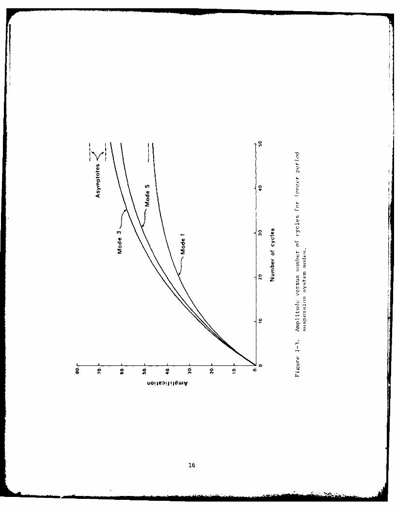
It is clear from the resonance curves that the long period input motion

is strongly amplified. However, it takes many cycles before these amplifi-

cations are achieved. Figure 1-3 shows curves of amplification versus number

of cycles; for example, it requires over 50 cycles to achieve 90% of the theo-

retical maximum for the 3.4 second mode. Therefore, seismic inputs must have

duration on the order of minutes (9 3 minutes for the 3.4 second mode) in

order to approach the maximum achievable amplification.

1.2 Alarm Distributions and Early Hypotheses

The distribution of seismic alarms over Wing V are shown in Figure 1-4

for both the Pocatello Valley and St. Elias earthquakes. The Pocatello Valley

event triggered alarms in over 42% of the wing on a clear swath trending south-

east. Because neighboring silos to the north and south were relatively unaf-

fected, this alarm pattern suggested a localized belt of ground motion enhance-

ment. In comparison, the St. Elias event caused alarms in 46% of the wing;

however, they were grouped in the southeast rather than across the wing.

14

-o r0 r

o cr.

jo~ae uo~~e:)j!ldw

15~

00

U)U

0.

c* E

0.

1C :

a 0 U C

to~~ in Vuoileoj~NdZ

16 -

Go~'~ IPOCATELLO VALLEY

-6-7

-~C 0- 3.,~

ca..

F i g u r e~~~ 1 4 D i t i u i n o s e m c a L a r s c u e y t e 1 7 o a e l

V a l l e y~ ~~ ~ a n 1 9 7 -t -a e a t q a e ( f o d a -p r o v i d e d

16-

......................................................

The Pocatello Valley event graphically illustrated the sensitivity of

Wing V to ground motion from distant earthquakes. Prompted by this, a number

of studies have been conducted to explain the anomalies. Two of these, con-

cerned principally with local site investigations, are described below.

A geologic literature search conducted by Riecker (1975) examined the

geology of the tri-state area of northeastern Colorado, southeastern Wyoming

and southwest Nebraska, encompassing Wing V. It concluded that no subsurface

geologic, structural or geophysical trends conformed to the pattern of af-

fected silos. Riecker postulated that perhaps the latest fluvial deposits

(Tertiary) were significant because the southeast flow trends approximately

matched the alarm pattern orientation. A second postulate concerned the struc-

tural shape of the Denver Basin and its ability to focus seismic energy along

the swath of affected silos. Neither postulate was supported at this stage

by quantitative data. The search revealed a great amount of geologic data

from oil and water well drilling logs in the northern Denver Basin. This

follows from the fact that it is the second oldest oil producing area in the

United States and that late Tertiary aquifers supply large amounts of ground-

water for extensive agricultural developments in the region. These and related

data will be described in detail in Section 2.

In 1978 a Wing V ground motion study was reported by Ossing and CrOIwCv

(1978). The authors observed that the majority of silos affected by the Poca-

tello Valley event were located in the High Plains, south of the southerly

Goshen hole escarpment, Figure 1-1 (- 200 meters of elevation change), while

the lowland silos north of the escarpment were relatively unaffected. Citing

evidence that motion is amplified near the top of a ridge and attenuated near

the bottom, Bouchon (1973), the authors instrumented two sites on either side

of the escarpment, one in Flight S and the other in Flight R. The seisio-:raph

18

stations were operated for one year, November 1976 to October 1977, and recorded

one earthquake with source location and magnitude approaching the Pocatello

Valley event (500 km away in eastern Utah, ML 5.0). There were no significant

differences in ground motion levels or missile effects between the two stations.

In addition, the authors examined seismic risk criteria for the Wing V area

and compared source characteristics from the Pocatello Valley event and

a 1975 Yellowstone earthquake (ML = 6.). The Yellowstone event did not

affect Wing V due in part to a favorable fault plane orientation and attenu-

ation through the Yellowstone caldera, both minimizing seismic radiation

towards the wing. Ossing and Crowley concluded that a source-site transfer

function was necessary in order to explain the anomalous Wing V effects.

Such a study is described in Section 1.3.

A seismic risk evaluation program was initiated by the Air Force in

response to the Wing V anomalies as well as the Palmdale uplift near Edwards

Air Force Base. Battis and Hill (1977) analyzed seismicity and tectonics of

the central and western US, including the Rocky Mountain region of interest

here. Recurrence relations and strain release maps were developed. The

Pocatello Valley event and a June 30, 1975 Yellowstone earthquake were ana-

lyzed using far-field surface wave data. It was noted that the effects at

Wing V might be explained by Rayleigh wave radiation patterns, although the

connection between seismic alarms and Rayleigh waves was not investigated.

Additional studies included the state of knowledge concerning the Palmdale

uplift in Southern California, and the state of earthquake prediction tech-

nology. In a second report, Battis (1978) conducted seismic risk studies of

three military facilities in the western US, including Wing V near Cheyenne,

Wyoming. These studies resulted in ground motion risk curves relating ground

motion levels to annual occurrence probabilities. However, thn paucity of

19

near-regional data limited the accuracy of risk evaluation for Wing V. A

recurrence period of two years for Wing V disturbances was predicted.

1.3 Source Modeling and Synthetic Seismograms

The Pocatello Valley earthquake was one of the best documented earth-

quake sequences in the Basin and Range province. The University of Utah's

telemetered seismic network and portable instruments deployed by the Uni-

versity and U.S. Geological Survey provided abundant details of the fore-

shock, mainshock and aftershock activity. The seismological data are dis-

cussed in detail by Arabasz, et al. (1980). The authors describe the earth-

quake sequence as a complex episode of Basin and Range graben subsidence that

may typify similar source regions elsewhere in the Intermountain Seismic

Belt.

In 1978 Day, et al. (1978) reported analytical and numerical source

models for the Pocatello Valley event. These were derived by constraining

the focal mechanism using the above-mentioned aftershock data and fitting

synthetic seismograms to observed long and short period teleseismic P

wave data. To fit the data, they had to include variable rupture velocity,

variable stress drop and unilateral rupture toward the free surface. In

a follow-on report Rodi, et al. (1979) used the above Pocatello Valley source

model and a simplified plane, layered path model to calculate synthetic

seismograms at Wing V. The overall effort described in these reports was

state-of-the-art and involved a successful unification of several rather

complicated analytical techniques. One purpose was to determine features

of the source or path which might make the event unique among western U.S.

earthquakes. Other research objectives not described here were synthetic

seismograms for western U.S. earthquakes in the range of 150-250 km, modeling

of the 1975 Yellowstone earthquake and initial comparisons of surface motion

generated by earthquakes and large surface explosions.

20

In the remainder of this section, the above synthetic seismogram cal-

culations for Wing V will be described. These were prompted by the lack

of measured ground motion data in the area of interest. The calculations

utilized generalized ray theory for the early arriving P waves, and modal

superposition for S waves and surface waves. Both techniques were coupled

to the analytical source model derived by Day, et al. (1980). Anelastic

shear attenuation was incorporated using an approximate Q operator. Ap-

proximations in the wave propagation analysis included the neglect of certain

weak body wave phases and truncation of modal sums at the fifth or sixth

higher overtone. The authors concluded that the analysis was probably adequate

for the source and epicentral distances involved. The path model used was

a Northern Colorado Plateau model from Keller, et al. (1976) based on short

period Rayleigh wave dispersion. The two kilometer sedimentary layer in

Lhis model was a rather crude approximation to the true propagation path

so another model without the layer was employed to bound its effect. Two

postulated Q models were also included to indicate the effect of anelastic

attenuation.

The best estimates of ground motions were for the model with a sedimentary

layer. Synthetics for the two cases are shown in Figure 1-5. Peak motion

at the closest of the Wing V sites are: displacement, 0.05 cm (tangential);

2velocity, 0.12 cm/sec (radial); and acceleration, 0.35 cm/sec (radial).

Corresponding values at a site 88 kilometers further southeast are about

half these. The principal difference between the synthetics with and without

a sedimentary layer is the surface waves. These are highly dispersed by

the surface layer and the Rayleigh wave is dominated by longer period motion.

Without the layer, the surface waves are much less dispersed yielding more

impulsive arrivals; in addition, the amplitudes are roughly doubled.

21

CM-

0O 0

.0 . . .Li o 0

Q)r

X "4j

NC M

Sj -, 0 L 0

i4 ir- . (V

0'

0 0 4

C

220

SECTION 2

GEOLOGICAL EVOLUTION OF THE WING V AREA

Wing V is distributed over the tri-state area of Wyoming, Nebraska and

Colorado in the northern Denver Basin. It is bounded to the west by the

Laramie Range of the Central and Southern Rocky Mountains and to the east by

the Great Plains of central North America. The principal tectonic features

are illustrated in Figure 2-1 from King, et al. (1969). The structure to the

west is dominated by the Cordilleran system of mountains, basins and plateaus,

which extends 800-1600 kilometers inland from the Pacific Coast along the length

of North America. The eastern part of the system was deformed most recently dur-

ing the Laramide orogeny towards the end of the Mesozoic era. For reference,

the geologic time scale is shown in Table 2-1. The principal source of informa-

tion on the evolution of the region is King (1977).

2.1 Tectonic and Geologic Background

The Laramide orogeny, beginning in late Cretaceous time, affected the

easternmost extreme of the Cordilleran, creating great vertical uplifts. Some

raised so high that cores of basement rock were brought to the surface. The

structures developed from rocks of the ancient continental platform previously

deformed in late Paleozoic time. The structures have since been modified by

processes during Tertiary time. These include the formation of basins soon

after the main orogeny, in which Tertiary sediments were deposited; and region-

al uplift of broad areas which is responsible for the present height of the

Central and Southern Rocky Mountains and Colorado Plateau. Streams invigorated

by the uplift have etched out the ranges of the Rockies and the myriad canyons

of the Plateau. A schematic illustrating structural evolution of the Front

23

m U

~~ z,

'0 .0 C-

0z

22

4,UOV ,

CK

00 1.) ; . SU

C.2 C1 Ci CLz 4J

0 O -) u

$00- o a)Maw --

z Q) - -,

"C0

-z 4 Q)

a 00

1 0.u u U. C.Oc c

U -

0 ~ 0M

00

0)-.

Table 2-1. Geologic Time Scale

BeganDuration in Millions

Era Period Epoch Millions in Years of YearsAgo

Cenozoic Quaternary Recent (Late archeologic andhistoric time)

Pleistocene 1 I

Tertiary Pliocene 12 13

Miocene 12 25Oligocene 11 36Eocene 22 58Paleocene 5 63

Mesozoic Cretaceous (Early, 72 135Jurassic Middle, or 46 181Triassic Late) 49 230

Paleozoic Permian (Early, 50 280Carboniferous: Middle, or

Pennsylvanian Late) 30 310and

Mississippian 35 345Devonian 60 405Silurian 20 425Ordovician 75 500Cambrian 100 600

Precambrian:Proterozoic 900 1,500

andArcheozoic (undetermined)

25

Range of Colorado is shown in Figure 2-2. Similar processes operated on the

Front Range's northerly extension, the Laramie Range in southeast Wyoming.

Figure 2-2a shows structure during late Paleozoic time, after formation of

the Front Range geanticline, an upwarping of platform sediments. Figure 2-2b

shows the situation in late Mesozoic time when the range was quiescent and

buried, followed by (c) in early Tertiary time immediately after the Laramide

orogeny. Figure 2-2d shows the present relations following later Tertiary

regional uplift and dissection. A more general illustration of the different

structural features found along edges of the uplifts is shown in Figure 2-3.

These include a dipping border along the core of exposed Precambrian rocks,

with the upturned sediments carved by erosion into lines of hogbacks (a); near-

ly vertical faults with Cretaceous and early tertiary rocks of the basin abu-

ting Precambrian rock faces (b); faults dipping under the mountains so that

Precambrian core rock is thrust over basin rocks (c); and lastly, all of these

borders covered by younger sedimentary dcposits which overlay the older rocks,

masking structure (d).

The regional tectonic map, Figure 2-1 shows the overall configuration of

mountains and basins as compiled by King. Heavily metamorphosed, steeply til-

ted Precambrian rocks form most of the cores of ranges in Colorado and Wyoming.

The Precambrian of the ranges in Wyoming are predominately a complex of para-

gneiss and orthogneiss. These rocks are truncated to the south by a northeast

trending shear zone (Mullen Creek - Nash Fork Shear Zone) south of which is a

metamorphic complex (paragneiss) forming the basement of the Southern Rocky

Mountains. Embedded in this complex and covering over half of the exposed

Precambrian is an array of granitic plutonic rocks (igneous intrusions).

During Cretaceous time a broad seaway extended north across the continent

from the Gulf of Mexico to the Arctic Ocean, along the eastern side of the

26

Front Range geanticline

A

B

C

Front Range

D

Figitre 2-2. Sections illustrating structural evolution ofthe Front Range of Colorado (from King (1977)).

27

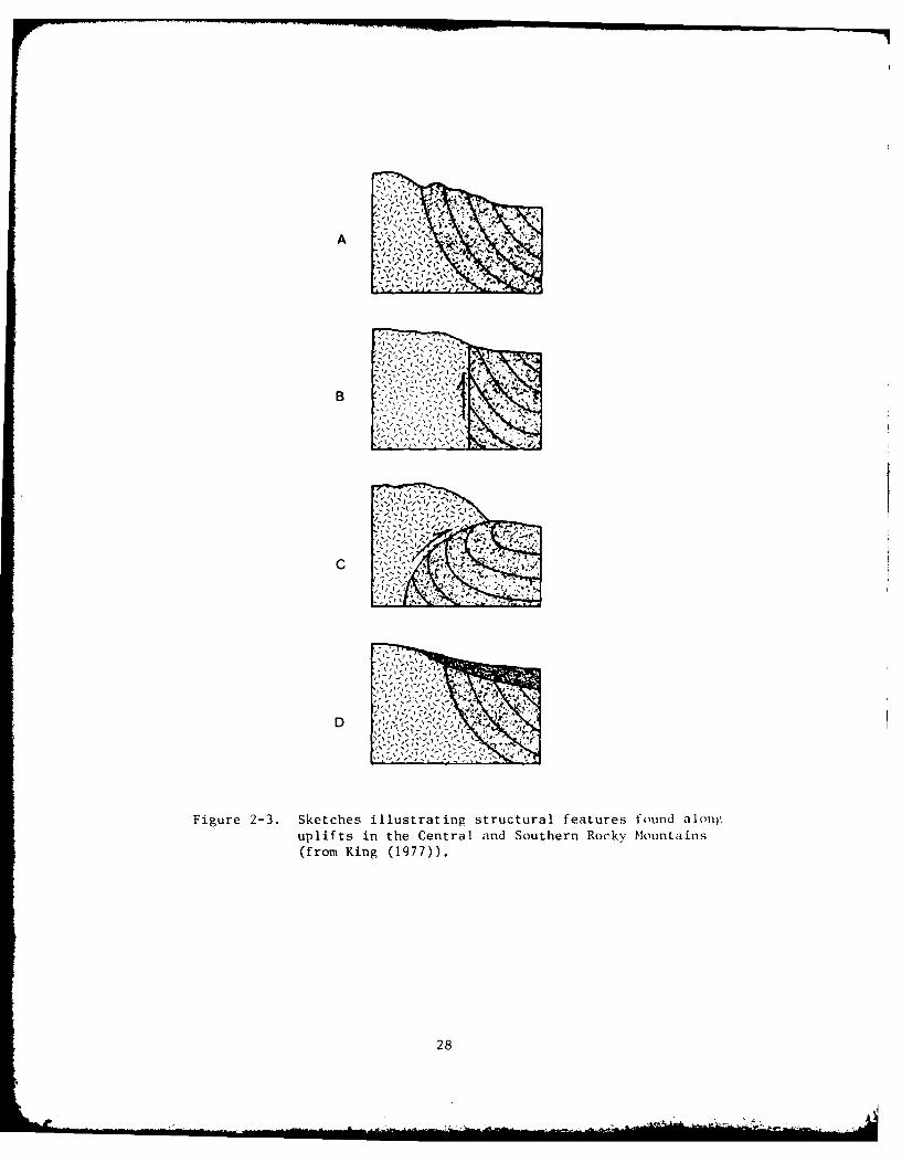
AB

Figure 2-3. Sketches illustrating structural features found alonguplifts in the Central and Southern Rocky, Mountains(from King (1977)).

28

Cordilleran region from central Utah to Kansas, Iowa and Minnesota. In Kansas

the Cretaceous deposits laid down in the seaway are no more than a kilometer

thick, beginning with a sandstone, the Dakota, overlain by interbedded lime-

stone and Niobrara Chalk below and the Pierre Shale above. Further west, near

the front of the Rocky Mountains, the deposits have thickened to 3 kilometers,

most of the incrase due to shales.

Overlying the main body of the earlier Cretaceous deposits are continental

(as opposed to marine) and coal bearing deposits of latest Cretaceous age.

These have a different pattern from the widespread earlier deposits and occur

in local basins such as the Denver, Powder River and Williston Basins, indi-

cated in Figure 2-1. The latest Cretaceous deposits were laid while the ranges

about them were uplifted, during the Laramide orogeny. The ranges did not pro-

ject in their present form but instead eroded as they were uplifted, shedding

detritus into the basins (see Figure 2-2c).

2.2 The Denver Basin

The Denver Basin is a shallow, sediment filled depression between the

front ranges of the Southern Rocky Mountains and the Great Plains. A structural

contour map is illustrated in Figure 2-4. The axis of the basin lies on a

line between Cheyenne, Wyoming and Denver, Colorado. West of the axis the

00basement has a moderate to steep dip (5 to 100+) while to the east the dip is

very shallow (< .5 0). The upper Denver Basin (Julesburg Basin) is bounded to

the west by the Front and Laramie Ranges, to the northwest by the Hartville

Uplift, and to the northeast by the Chadron Arch. The area geology and tec-

tonics have been studied intensively because it is one of the oldest petroleum

producing provinces on the continent and still holds promise of additional re-

serves. The Cretaceous reservoirs are the most important, followed by

29

CHAD RONARCH

S -1000

ARHA

Z,0

rok Dne envrBsn otus r nfe eo

se lve (n at ro Mt o~..:k C)b

30A

accumulations in older rock (see Cram (1971)). Additionally the Tertiary de-

posits are an important source of ground water and numerous water resource

studies have been done (see Rapp, et al. (1957)).

Structure surrounding the upper Denver Basin will be described briefly

(see Anderman and Ackman (1963)). The mountain flank structure north from the

Wyoming-Colorado bbrder along the Laramie Range is a series of high angle thrust

(reverse) faults continuing to the northeast trending fault zone on the south-

east flank of the Hartville uplift (see Figure 2-1). The Hartville uplift is

a doubly plunging structural high extending northeast from the Laramie Moun-

tains to the southwest flank of the Black Hills and separates the Powder River

and Denver Basins. To the northeast is the Chadron Arch (Chadron-Cambridge),

a major structural feature trending northeast-southwest from the Black Hills to

the central Kansas uplift.

A more detailed discussion of the faulting along the flank of the Hartville

uplift is provided by Droullard (1963). During Miocene and Pliocene time addi-

tional uplifting of the Laramie Range, including the Goshen Hole area, Figure

1-1, occurred. When compression ceased, the northwest flank of the Goshen up-

lift collapsed forming the fault system indicated on the tectonic map, prin-

cipally the Whalen and Wheatland faults of the Richeau-Jay EM fault zone. The

Whalen fault has a net vertical displacement of 1.5 kilometers in Paleozoic

rocks. It is a thrust fault in the Cretaceous and older rocks and a normal

fault with 250 meters of displacement in Tertiary deposits.

Stratigraphy in the Denver Basin has been described in great detail in the

geologic literature. An extensive catalog and description of formations is

included in Bolyard and Katich (1963). Anderman and Ackman (1963) present a

structural contour map of the Denver Basin based on all wells which bottomed

in Mississippian or older rocks. Combining this data with isopach (thickness)

31

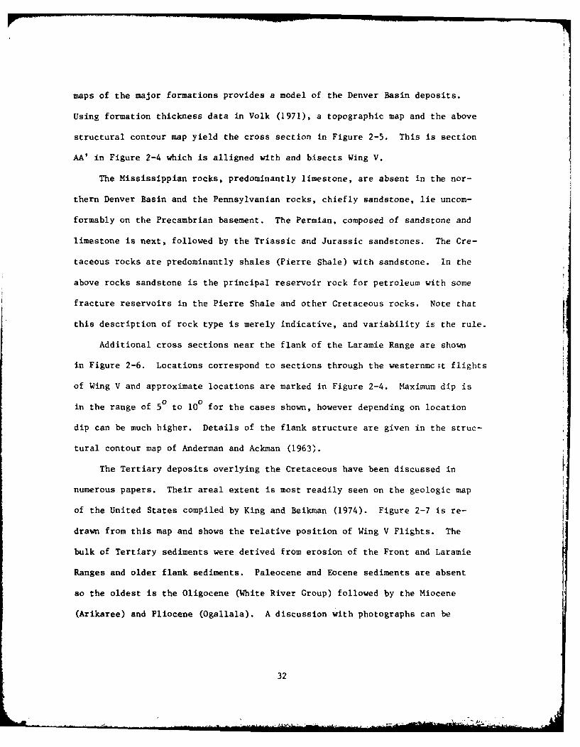
maps of the major formations provides a model of the Denver Basin deposits.

Using formation thickness data in Yolk (1971), a topographic map and the above

structural contour map yield the cross section in Figure 2-5. This is section

AA' in Figure 2-4 which is alligned with and bisects Wing V.

The Mississippian rocks, predominantly limestone, are absent in the nor-

thern Denver Basin and the Pennsylvanian rocks, chiefly sandstone, lie uncom-

formably on the Precambrian basement. The Permian, composed of sandstone and

limestone is next, followed by the Triassic and Jurassic sandstones. The Cre-

taceous rocks are predominantly shales (Pierre Shale) with sandstone. In the

above rocks sandstone is the principal reservoir rock for petroleum with some

fracture reservoirs in the Pierre Shale and other Cretaceous rocks. Note that

this description of rock type is merely indicative, and variability is the rule.

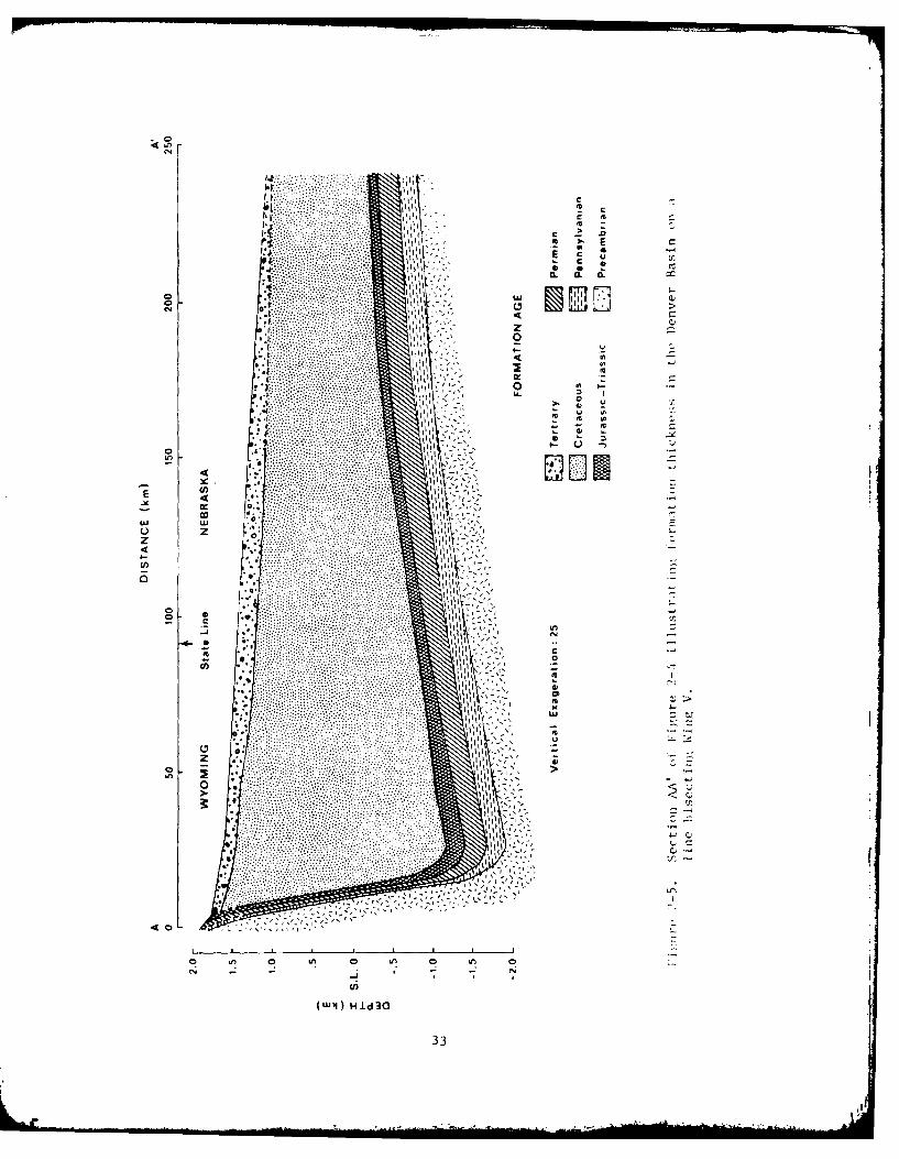
Additional cross sections near the flank of the Laramie Range are shown

in Figure 2-6. Locations correspond to sections through the westernmc~t flights

of Wing V and approximate locations are marked in Figure 2-4. Maximum dip is

in the range of 50 to 100 for the cases shown, however depending on location

dip can be much higher. Details of the flank structure are given in the struc-

tural contour map of Anderman and Ackman (1963).

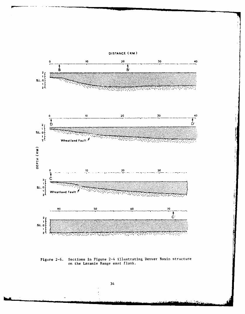
The Tertiary deposits overlying the Cretaceous have been discussed in

numerous papers. Their areal extent is most readily seen on the geologic map

of the United States compiled by King and Beikman (1974). Figure 2-7 is re-

drawn from this map and shows the relative position of Wing V Flights. The

bulk of Tertiary sediments were derived from erosion of the Front and Laramie

Ranges and older flank sediments. Paleocene and Eocene sediments are absent

so the oldest is the Oligocene (White River Group) followed by the Miocene

(Arikaree) and Pliocene (Ogallala). A discussion with photographs can be

32

llil

till -4

..........

111

... ... ... ... L

0

4Y.lilt~

E .. ...... ...

z. hipu

. ... ..

C

............ ..0. . .

lilt,

DISTANCE (KM)

010 20 30 40

B B'

&L. 0

0 10 20 30 40

2 D D

S.L. 0: . . . .. i. . .

0.

0 10 20 30

SL Wheatland Fault ;-- Z- , '. .. S7 ,-

40 s0 60 70

Figure 2-6. Sections in Figure 2-4 illustrating Denver Basin structureon the Laramie Range east flank.

34

0 0

Lu 4O1 00 45 tM4 aMi

0 0 -

SE31E E n~ 11 E]

I4)

cJ a)

35

found in Moore (1963). The topography of Cretaceous sediments underlying the

Tertiary is probably much like the Colorado Piedmont of today, i.e. a dissected

irregular plane, predominantly shale, as described by Harris (1963).

The Oligocene White River Group is composed of the older Chadron member

underlying the Brule member. These rocks were deposited on an erosional sur-

face and were eroded in turn, thus total thickness may vary from 0 to 200 meters

over short distances. The Chadron formation is highly variable consisting of

siltstones, sandstones and conglomerates with thickness up to 50 meters. Above

the Chadron are massive clays and siltstones making up the Brule formation,

with thickness from 0 to 150 meters. The Brule is hard and cut by fractured

zones, fissures and faults. It weathers into a badland topography but when

protected by resistent younger beds forms steep cliffs like the Goshen Hole

escarpment.

Miocene sediments are referred to here as the Arikaree. There is some

confusion in the literature as to a consistent designation, but these rocks

are for the most part siltstones and volcanic ash with a maximum thickness of

25 meters. A thin layer of Arikaree appears to form an effective cap rock for

the Brule along escarpments.

Capping the High Plains is a series of sandstones, conglomerates, silt-

stones and limestones of Pliocene age which are included in the Ogallala forma-

tion. Thickness varies from C to 90 meters. Grain size decreases eastward

from the mountains. Near the Laramie Range the Ogallala is a poorly sorted

conglomerate with boulders a meter or more in diameter. In eastern Wyoming it

is a well sorted sandstone and siltstone. The conglomerate contains fragments

of nearly every rock type in the Laramie Range.

By the end of the Pliocene epoch a vast sheet of alluvium extended from

the front ranges east onto the Great Plains. Only a remnant of the blanket has

36

survived the severe dissection that characterized Quaternary time. This is

clearly seen in Figure 2-7. The major remnant is the Gangplank of the High

Plains where the mountains-plains surface is continuous. Historically the

Gangplank provided a natural route over the Laramie Range. Isopach maps of

Pliocene, Miocene and Oligocene rocks in the tri-state area have been compiled

by Denson and Bergendahl (1961). A section schematic through Wing V is shown

in Figure 2-8a along with a sketch of a local section in Banner County, Nebraska

illustrating the variability of formation thicknesses, Figure 2-8b.

The Tertiary deposits exhibit variable degrees of cementation from carbo-

nates and to a lesser extent silica. These cemented areas are more resistent

to erosion than the softer areas and form well defined ledges and escarpments.

These features can be seen quite clearly in Landsat imagery of the region pro-

vided by Smith, et al. (1980). The escarpments are most prominent along Wild-

cat Ridge and the southwestern Goshen Hole area indicated in Figure 1-1, and

provide up to 200 meters of vertical relief in the Arikaree and White River

formations. Farther south the escarpments are found on either side of the

Ogallala forming the Gangplank to the Laramie Range. On the north side the

vertical relief is probably no more than 90 meters while to the south it may

be on the order of 60 meters. Lesser rellet features are common due to stream

dissection, and Landsat pictures indicate a correlation with the distribution

of Tertiary sediments shown in Figure 2-7.

37

(Moee 6000±ft

B.500 300

4505+00

400000

od ~ ~ ~ ~ ~ Per PeShSalerd~ ~rn~os. )"WIN 600 f

Figure 2-8b. Achnortc suhown se tonthrugh reltin B f illus rtig . r,,

oasetothogWigV(from Senith and Souders (1975)

(196138

SECTION 3

GROUND MOTIONS FROM THE POCATELLO VALLEY AND ST. ELIAS EVENTS

Ground motions at Wing V from the Pocatello Valley and St. Elias earth-

quakes are not known with any certainty. The synthetic seismograms calculated

by Rodi, et al. (1,979) for the Pocatello Valley event provide the only avai-

lable estimate of ground motion within the wing. However, seismograms are

available from the seismograph station at Golden, Colorado, about 200 km south-

west of the wing, within the Denver Basin. These records will be discussed

here to compare and contrast motions from the two events. Observations

have been overshadowed by the calculational approach in most considerations

of Wing V anomalies. Recognizing that seismic alarms will probably be trig-

gered by future earthquakes, the collection and interpretation of relevant

seismograms is an important complement to ground motion calculations.

3.1 The St. Elias Earthquake

The St. Elias earthquake occurred on February 28, 1979 in southeast Alaska

near 60.6 N, 141.6 W with a surface wave magnitude, M. = 7.1 reported. The

source was shallow, averaging about 11 km and the earthquke ruptured approxi-

mately 60 km to the southeast in three subevents with individual ruptures esti-

mated at 12, 27 and 17 km , Boatwright (1980). The propagation path from south-

east Alaska to the Wing V area was entirely continental, along the Cord]leran

System, the mountain belt of western North America. Most of the path followed

the demarcation between mountains and interior continental plains. Distance from

the epicenter to Wing V was about 3350 km (A=300) and the azimuth was approxi-

mately 380 northwest from Wing V.

39

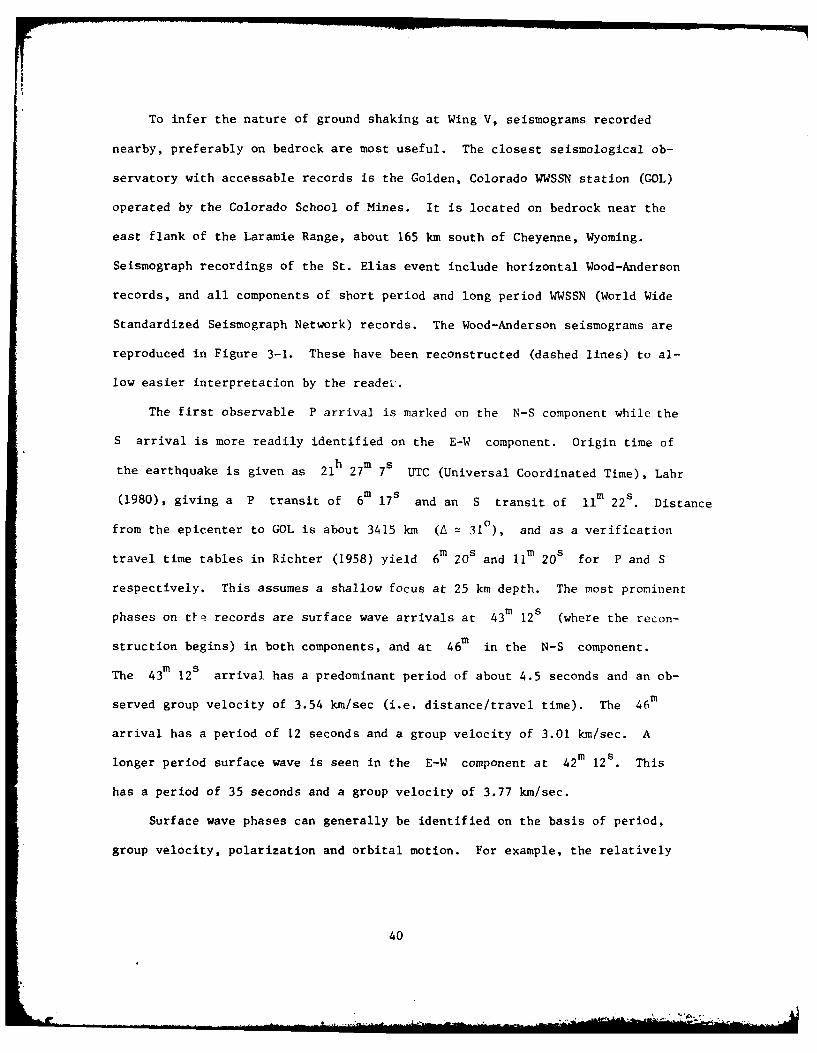
To infer the nature of ground shaking at Wing V, seismograms recorded

nearby, preferably on bedrock are most useful. The closest seismological ob-

servatory with accessable records is the Golden, Colorado WWSSN station (GOL)

operated by the Colorado School of Mines. It is located on bedrock near the

east flank of the Laramie Range, about 165 km south of Cheyenne, Wyoming.

Seismograph recordings of the St. Elias event include horizontal Wood-Anderson

records, and all components of short period and long period WWSSN (World Wide

Standardized Seismograph Network) records. The Wood-Anderson seismograms are

reproduced in Figure 3-1. These have been reconstructed (dashed lines) to al-

low easier interpretation by the reader.

The first observable P arrival is marked on the N-S component while the

S arrival is more readily identified on the E-W component. Origin time of

the earthquake is given as 21h 27m 7s UTC (Universal Coordinated Time), Lahr

(1980), giving a P transit of 6m 17s and an S transit of 1im 22s . Distance

from the epicenter to GOL is about 3415 km (A = 310), and as a verification

travel time tables in Richter (1958) yield 6m 20s and 11m 20s for P and S

respectively. This assumes a shallow focus at 25 km depth. The most prominent

phases on tle records are surface wave arrivals at 43m 12s (where the recon-

struction begins) in both components, and at 46m in the N-S component.

The 43m 12s arrival has a predominant period of about 4.5 seconds and an ob-

served group velocity of 3.54 km/sec (i.e. distance/travel time). The 46m

arrival has a period of 12 seconds and a group velocity of 3.01 km/sec. A

m slonger period surface wave is seen in the E-W component at 42 12 . This

has a period of 35 seconds and a group velocity of 3.77 km/sec.

Surface wave phases can generally be identified on the basis of period,

group velocity, polarization and orbital motion. For example, the relatively

40

--- - --------

-- z =

r E VI

CI-In

In

z -

z E z) - i0 z

0o 0.

U 0 0

j E I.0-

0) 0

00 0

0 )

i- 0

C4 N

41-

short period and group velocity of the 43m 12 arrival identify it as Lg,

a phase which is routinely observed on strictly continental paths over North

America. Lg is generally regarded as a complex of higher mode surface waves

propagating within a crustal waveguide at nearly the granitic shear velocity

of 3.51 km/sec or so (Ewing, et al. (1958)). Unlike fundamental mode surface

waves, where the highest amplitudes occur at or near the surface, the Lg

phase carries most of its energy deeper within the crust. Consequently it is

less disturbed by surface structure and is often the dominant phase on a

seismogram.

The highest amplitude surface wave arrival, at 46m in the N-S record,

is a Rayleigh wave. This follows from observed dispersion curves for continen-

tal Rayleigh waves shown in Figure 3-2a, from Ewing, et al. (1958). One of the

data points, a seismogram from a March 1, 1955 Yukon aftershock recorded at

Palisades, New York, is shown in Figure 3-2b from the same reference. Comparing

the 1979 St. Elias N-S record to the 1955 Yukon aftershock N-S record shows

a striking similarity. The Lg phase from the 1955 event has a period of

about 4 seconds (compare to 4.5 seconds for the 1979 event) and the Rayleigh

wave, designated Rg, has an initial 8 second period (compare to 12 seconds).

Rg was identified at Palisades by orbital motion and group velocity. The Rg

phase in Figure 3-2b is also notable because it exhibits reverse dispersion,

where shorter periods lead longer periods in contrast to normal dispersion. The

travel path from the Yukon epicenter to Palisades is about 4250 km based on travel

time. Similar phasing between Lg and Rg for the two events is due to the

greater distance in combination with a slightly higher group velocity of Rg

recorded at Palisades. Referring back to Figure 3-1 note that the E-W compo-

nent of ground motion from the 1979 event does not show the Rg phase.

42

4.5- -

4.0 -

35 km. 6 -3 51 krm/sec- 0 0000

P, -4.66 km./sec.~3.5 212o 4 00 i

3.0 IfCL a Yukon to Palisades, New York 1 March 1955

0 Algeria to Natal 9 September 1954 01-04-37

2.5 4 Algeria to Natal 10 September 1954 05-44-05*California to New York (Brit~ant and Ewing)

o Mantle Rayleigh Wave (Ewing and Press)

2.0 - . IIW.I .. I. II.0 10 20 30 40 50 60 70

Period in seconds

Figure 3-2a. Observed and theoretical dispersion of continentalRayleigh waves (from Ewing, at al. (1958)).

1Mar c T0 W10IMA5 -

14022514:24

Yu!'on Aftershock

Figure 3-2b. Palisades NS seismogram of Lg and Rg waves fromYukon aftershock of March 1, 1955 (from Ewing,et al. (1958)).

43

This is consistent with the polarization of Rayleigh vave ground motion al-

though some E-W component would be expected considering that the azimuth at

GOL is 380 northwest.

Longer period surface 2dves can also be identified. Figure 3-3 shows a

composite of dispersion curves for Love and Rayleigh waves. The 35 second

E-W arrival at 42m 12s fits the curve for continental Love waves and is

designated LQ. The 18 second motion in the N-S component probably corres-

ponds to a continental Rayleigh wave arriving close to the Rg Rayleigh wave.

Body waves are much weaker phases than surface waves at distances consi-

dered here, 300 or so. This is primarily due to the three dimensional spread

of body wavefronts as compared to the two dimensional spread of surface waves.

The Wood-Anderson and short period WWSSN seismograms from GOL are used here to

examine body wave arrivals. Between the P and S arrivals marked on thf Wood-

Anderson seismograms the travel time curves (e.g. the Jeffreys-Bullen tables,

Bolt (1976)) show multiple mantle reflection (PP,PPP) and a core reflection

(P cP) of longitudinal (P) motion. Between S and the surface waves are

additional transverse (S) body wave arrivals (P cS , SS, etc.). Rather than at-

tempt an identification of these phases a brief discussion of the period and

amplitude history will be given.

Counting peaks on the Wood-Anderson seismogram between P and S yields

an average period of body wave motion of 3.5 seconds. A corresponding section

of the short period WWSSN seismogram (not pictured here) indicates significant

motion down to I second but because of excessive gain and the superposition of

later arrivals it is difficult to determine a predominate period or range of

periods. The situation is somewhat clearer after the S arrival where the

spacing of peaks indicate periods in the range 3 to 6 seconds. At the Lg

44

0 0-

0 0r

01 -

00. o00

c-4

0 L

0I.

000 0

0 - IM

C0 0

C\jQC

0)~

-C.- IM,

z4 >

C4

C...) Cc

U.,

0 00 0 r:

( 4s/~) CL3O3 >fO

45E

v--------------

arrival, periods in the range 2 to 3 seconds appear to be superposed on the

4.5 second Lg motion.

Few strong conclusions can be drawn from the above short period body wave

observations. Suffice it to say that overall, body wave arrivals with periods

in the range of interest, 2 to 6 seconds are present in the seismograms. Due

to excessive gain no amplitudes can be measured with confidence from the short

period seismograms, however the N-S component of Wood-Anderson record, Figure

3-1 indicates a peak P wave motion of .1 millimeter at a period of 4.8 seconds.

3.2 The Pocatello Valley Earthquake

The Pocatello Valley earthquake sequence of late March and April of 1975

was centered near the Idaho-Utah border at 42.1 0 N, 112.5 0 W. The sequence in-

cluded a magnitude 4.2 (ML) foreshock, a 6.0 mainshock, one 4.7 and two 3.8

aftershocks and over 50 lesser events greater than 3.0. The sequence is des-

cribed in detail by Arabasz, et al. (1980) who attributed the events to irre-

gular Basin and Range graben subsidence within the Pocatello Valley. The pro-

pagation path from Pocatello Valley to the Wing V area was nearly due east

across the lower third of Wyoming, a distance of about 700 kilometers. The path

included 180 km of the Idaho-Wyoming Overthrust Belt, 350 km of the Green

River Basin of Wyoming and about 170 km of the Laramie Range and the Denver

Basin. The tectonic map, Figure 2-1 shows these features and - rrounding struc-

ture. The epicenter is marked by a star on the border above the Great Salt

Lake.

The Pocatello Valley earthquake was a local event in contrast to the dis-

tant St. Elias event. Consequently the character of ground motion at Wing V

should differ. This is clearl7 seen in a comparison of time scales for the

46

I!

synthetic Pocatello Valley seismograms in Figure 1-5 and the Wood-Anderson

record of the St. Elias event in Figure 3-1.

Long and short period WWSSN seismograms recorded at the Golden, Colorado

station will be used here to infer general features of ground motion at Wing

V. The epicentral distance to GOL is 650 km and the azimuth is 660 east of south.

h m sThe main Pocatello Valley event, ML = 6.0, at 2 31 6 , March 28, drove the

long and short period records off scale at GOL for 4 to 5 minutes. Predomi-

nant periods could not be determined. However the lesser events provided good

records. The short period E-W seismogram of the first 3.8 magnitude after-

shock is shown in Figure 3-4. The sequence of arrivals seen here is common to

the 4.2 foreshock and the 4.7 aftershock. The first arrival, at 1m 32s af-

ter the origin time of 16h 15m 6s , March 28 is the P phase, a low ampli-

n

tude refracted wave from the Moho discontinuity. This is followed by the

higher amplitude P phase, a direct wave propagated through the graniticg

crust. Another arrival associated with intermediate layers in the crust may

be present between Pn and P . The next obvious arrival is Sg, the direct

shear wave through the crust. Faster refracted phases preceed this arrival

but are not obvious on the record. Also Love waves including Lg may be

superposed on S but no distinctions are obvious. The time between P andg g

S is 1m 16s . The spacing of peaks on the record indicate periods on theg

order of I second. The corresponding long period record shows no evidence of

this event.

The only significant long period record at GOL, besides the mainshock, is

the magnitude 4.7 aftershock, shown in Figure 3-5. The origin time is 13h

1m 2O h m1m 20s , March 29. The long period arrival at 13 5 has a travel time of

3m 40 s. The Z and E-W components have the higher amplitudes. Periods start

47

cmI

-~~F .5 5 - -

E 0c

00r

F- G)

*0O

C) C

U4

41

0 0

'n-4

7E E -4

ow0- co

t $-4 P4

10~C U 04

co

0 C-

Z02

0 0

W-4 4-i

0

o o

toJ w -H-

1~ -,4 U "

-0-,4

bo 4j

000)

49r U.

a) a)4*

at 12 seconds and after 1' 30s are down to 5 seconds. This behavior, the

normal dispersion and the particle motion in the Z and E-W directions,

suggests that this phase is a Rayleigh wave. Group velocity of the 12 second

period is found to be 2.95 km/sec, very close to the measured values in Figure

3-2a for continental Rayleigh waves. Apparently the smaller shocks do not

excite surface waves very efficiently; however, the 4.7 aftershock is seen to be

an effective source and the main shock is no doubt a very rich source.

Examining the synthetic seismograms in Figure 1-5 shows that these ob-

servations at GOL are consistent with calculated body and surface wave arri-

vals at Wing V. The synthetics are for an epicentral distance of 680 km com-

pared to 650 km at GOL. The first arrival in the synthetics is 95 seconcls

after the event, followed by higher amplitude P phases which precede the

higher amplitude S phases by about 85 seconds. Depending on the near sur-

face crustal model chosen, Rayleigh wave arrivals are between 210 and 240 se-

conds in the synthetics, compared to 220 seconds from the long period record

of the 4.7 aftershock. Allowing for the 30 km difference in epicentral dis-

tance would give an observed Rayleigh wave arrival at 230 seconds. This arri-

val time and the dispersed nature of the observed Rayleigh wave suggests that

the crustal model with a surface sedimentary layer is more representative of

the travel path from Pocatello Valley to Wing V.

A cross section through the travel path in Wyoming is shown in Figure

3-6 . This was compiled from a tectonic map of North America, King (1969) and

a state topographic map. It shows a substantial sedimentary cover over Pre-

cambrian basement which thins to the east, terminating on the west flank of the

Laramie Range. The section is located near a line connecting the Pocatello

Valley epicenter and a point 50 km north of Cheyenne, Wyoming on the tectonic

50

NEBRASKA:

WYOMING

N N%

E

N N U

Uz

WYOMIN zIDAH 40 qr 0 c, V 0 0 w C . <

(- )spp I

05

map, Figure 2-1. The behavior of surface waves propagating across such struc-

tures is unknown, both because the path includes sections with significant up-

dip and the presence of basement uplifts north and south of the path may chan-

nel surface wave energy. Shorter period surface waves have wavelengths com-

parable to the sediment thickness and therefore interact more readily with

the irregular path structure than would longer period surface waves. Also,

the upcLpping sediment cover on the west flank of the Laramie Range would be

expected to have a significant effect on shorter period sedimentary surface

waves. A uantitative evaluation of these phenomena is the subject of a

continuing effort on surface waves in sedimentary basins and will be reported

later.

52

SECTION 4

VELOCITY STRUCTURE IN THE DENVER BASIN

An understanding of surface ground motion over the Denver Basin begins

with a realistic seismic velocity model of the basin sediments. Sources of

data can include direct, local measurements such as velocity logs of wells,

seismic reflection and refraction surveys, laboratory testing of rock samples,

etc. Additionally, velocities can be inferred from data collected in similar

lithologies (rock types) in other areas, particularly the ubiquitous shales

and sandstones. In this section the available data will be described and ap-

plied to a generalized velocity model of basin deposits consisting chiefly of

shales and sandstones.

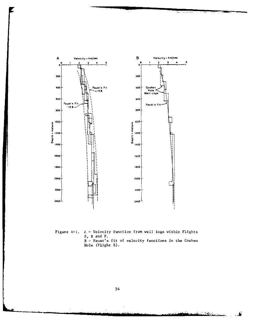
4.1 P Wave Models

The most readily available velocity data in the Denver Basin are P wave

well logs. These are obtained using a sending and receiving unit (sonde)

lowered down the well to measure interval transit time as a function of depth,

Telford, et al. (1980). The major limitation in using such logs to estimate

seismic velocities is their restricted sampling region around the borehole and

the unknown structural disturbance caused by drilling. Nonetheless these velo-

city logs are a useful source of P wave data in the absence of alternate

seismic velocity meausrements. Figure 4-la shows a collection of velocity

functions from five wells within Flights S, R and P in Wyoming (see Figure

1-1), as interpreted by Smith, et al.(1980). Independent spot checks of rele-

vant well logs from Nebraska and Colorado fall within the bounds indicated

in the figure.

A determination of velocity functions from well logs on a site by site

basis is beyond the scope of this investigation. The question is then, how to

53

A Velocity - kni/sec B Velocity - km/sec

0 1 2 3 4 5 0 I 2 3 4

0 T

200 - 200

400 - Fausts Fit 400 Goshen.ii Hole

Well Logo

600 -0

Faust's Faust's Fit

800 - 80

*1000 - 1000 ,

1200 - 1200

*I a

1400 - 1400

1600 i 1600

1800 1800

2000 - 2000

2200 - 2200

2400 2400

Figure 4-1. A - Velocity function from well logs within Flights

S, R and P.B - Faust's fit of velocity functions in the GoshenHole (Flight S).

54

**%'-i

generalize the limited data in Figure 4-la to the entire Wing V area consider-

ing the common lithologies and known formation depths? Similar questions con-

cerning the fullest utilization of well logs have been addressed by a number

of researchers over the years. For example, Haskell (1941) explored the rela-

tion between depth, lithology and velocity logs in Tertiary sandstones and

shales. He found a mean vertical velocity gradient of .464 meters/sec/meter,

and that on the average 78% of the gradient is due to overburden, the remainder

due to age of the formation. The effect of overburden on shales is smaller

than the average,while for sandstones it is larger. A crude comparison can be

made with the data in Figure 4-1a where the mean velocity gradient is .43 km/

sec/km for the interval between I and 2 kilometers depth.

A more extensive and applicable study of the question is found in Faust

(1951), where velocity functions were developed for shales and sandstones of

Pennsylvanian age and younger. The data used in the study came from over 500

velocity logs in the United States and Canada. Velocity was correlated with

depth and age, and interval velocities were plotted as a function of depth for

each age group. Log-log plots showed a common slope cf 1/6 for all curves

indicating that the velocity function could be fit by AZ , where Z is depth

and A is a constant depending on geologic age. The constants determined by

Faust were A(Cretaceous) = 967, A(Jurassic-Triassic) = 1047, A(Permian) = 1063

*and A(Pennsylvanian) = 1318 (modified from Faust's to yield velocities in

meters/second for Z measured in meters). The range of depths sampled was

300 to 3500 meters and Faust found reasonable agreement outside this range as

well. Sandstone velocities were about 100 m/sec greater than shale velocities

on the average.

An interesting note regarding Faust's fit of shale and sandstone is that

* such a relation is theoretically consistent with the theory of elastic waves

55

through a packing of small spheres, Gassmann (1951). Gassmann examined a

porous solid consisting of a hexagonal close packing of equal spheres, with

and without a fluid filler, using Hertz's theory of contact. Expressions were

developed for the P wave velocity as a function of depth when the packing

was stressed by self weight only. The velocity relation was found to be

V = AZ1 /6 where A is a function of Young's modulus, Poisson ratio, sphere

and fluid density and the acceleration of gravity. An example was given for

granitic spheres with the pore space dry or filled with water. The numerical

value determined for A(saturated) was 865, about 10% lower than Faust's value

for Cretaceous shale and sandstone. Another significant finding concerned

anisotropy. At a depth of 200 meters horizontal velocity was about 16% lower

than the vertical velocity for the wet case and the difference increased with

depth. No cross-hole tests are available to confirm this in the Denver Basin

however some anisotropy should be expected.

To compare Faust's velocity function with available data in the Denver

Basin consider the two curves shown in Figure 4-1b inferred from well logs 20

kilometers apart in the Cretaceous section of Flight S in the Goshen Hole area.

Taking mean velocity at a depth of two kilometers as the datum gi'es 3500 m/sec

from which A = 987. This is 2% higher than Faust's estimate based on a wide

variety of Cretaceous shales and sandstones. The fit is also plotted in Figure

4-1b and is seen to agree fairly well with log inferred velocities to a mini-

mum depth of 50 meters. Above this depth the velocities are too low.

There remains the question of velocity models in the Tertiary section

overlying the Cretaceous and older sediments modeled above. A search of

non-classified data showed that near surface velocities were determined

prior to construction at each of the 200 Wing V silo sites by Porter and

56

O'Brien (1960) using uphole and refraction surveys. Telford, et al. (1980)

describe the techniques. The velocity data is distributed through 20 volumes

(one per flight) of Wing V geologic and geophysical reports. A review of the

data shows that despite the unconformities and nonuniform thicknesses of the

Tertiary strata described in Section 2 there are no notable near surface

velocity anomalies below the surface weathered zone (5 - 10 meters deep).

Below a depth of 40-50 meters the P wave velocity is on the order of

2 + .5 km/sec. Above this level velocity structure can be classed as slow,

moderate or fast, describing a surface layer 20-30 meters thick with velo-

city around 1000, 1500 or 2000 m/sec respectively. Assigning a numerical valut

of -1 to slow sites, 0 to moderate sites and + I to fast sites and sum-

ming over each flight results in the distribution indicated in Figure 4-2. N

is the numerical sum at each flight. Referring back to the geologic map,

Figure 2-7, a comparision shows that slow, moderate and fast sites correlate

with Pliocene, Miocene and Oligocene surface deposits respectively. The corre-

lation is not perfect but it serves to demonstrate that near surface velocities

correspond fairly well with near surface geology. Of course many other factors

can perturb surface properties including depth to groundwater, soil overburden,

cementation, etc. Depth to groundwater is probably the next factor to consider.

Groundwater surveys published by the U.S. Geological Survey are a rich source

of data. However for the purpose of this investigation suffice it to say that

the depth depends on the surface elevation and is generally greater for high-

land and lesser for lowland. Average water depth is around 40 meters which is

on the same order as expected surface relief.

57

(n L - I

V V I t

0)

WWVeN VIV Va-J ~

LuL

Uc - ZU 0

Cfl I I0 0

00

C~~~~ ~ ~ ~ -- -----

* ,, * .- , N

58

4.2 S Wave and Density Models

The above data provide a reasonable model of the P wave velocity func-

tion in the Denver Basin deposits. This model is consistent with velocity logs

of wells in the area and also with logs in similar lithologies at comparable

depth elsewhere in the United States and Canada. However, a complete seismic

velocity model must also include S wave velocity and density functions. For

this purpose the available data come from laboratory tests of rock samples and

empirical relations developed in geophysical exploration.

Geophysical testing of rock samples under laboratory controlled conditions

of pressure, saturation, etc. is a valuable source of data, particularly in

conjunction with field observation. A timely example is preliminary data pro-

vided by Tosaya (1980) on recent laboratory tests of Pierre Shale samples from

a South Dakota oil well in Williston Basin sediments. Sediments in the Denver

and Williston Basins have the same depositional history and test results should

indicate common properties. Core samples provided by Tosaya included a shale

specimen from 1 km depth which was clayey in appearance with a gritty fracture

surface and many small fossil fragments; another shale specimen from 1.5 km

depth was dark and hard, appearing more rock like with no fossil fragments in

evidence; and a third specimen from 2 km depth, with an appearance somewhere

between the previous two, turned out to be virtually all limestone. Laboratory

velocity measurements were made on the 1.5 km shale specimen and some of

Tosaya's results are shown in Figure 4-3. Samples were either dry or saturated

with deionized water, confining pressure ranged from atmospheric to 1.2 kilo-

bars (1216 atmospheres) and a maximum pore pressure of 410 bars was applied.

Figure 4-3a shows P and S velocities, Vp and VS, for dry and saturated

Pierre Shale. Velocities increase rapidly with confining pressure at low

pressures due to closure of microcracks and the resulting decrease in porosity.

59

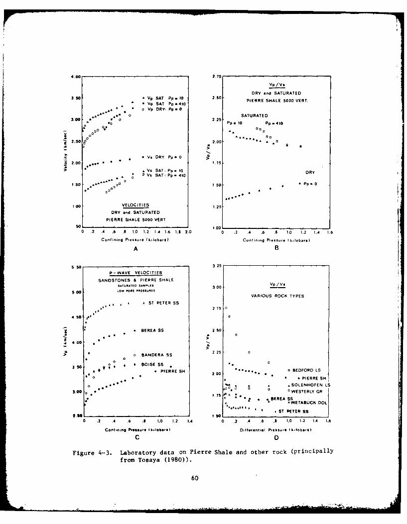
4.00 .2.75

Vp /Vs

DRY and SATURATED3.50 AVp SAT: Pp. 10 2.50- PIERRE SHALE 5000 VERT.

*Vp SAT: Pp.A,410A o Vp DRY: Pp.0

.A 0 SATURATEDA .022 Pp. 10 Pp -410

2.50 2.00 A

*Vs DRY Pp 0 C

S2.00 A~ t .75

> VS SAT: Pp.10 DRYA a Vs SAT Pp. 410

1.0 .A." a0

1.50 *Pp. 0A OD

100 VELOCITIES 1.25DRY and SATURATED

PIERRE SHALE 5000 VERT

so100 .2 .4 .6 .8 1.0 1.2 1.4 1.6 1.6 2.0 000 .2 .4 .6 .8 1.0 1.2 1.4 1.6

Confining Pressure (k~iobars) Confining Pressu~re I kilobarsI

A B

5 50 3 325

P-WAVE VELOCITIES

SANDSTONES & PIERRE SHALESATURATED SAMPLES 3 00VpV

5.00LOW osE SESSIESVARIOUS ROCK TYPES

* ST PETER SS272 7

*BEREA SS 2 50

E >4 00 *

ch o BANDERA SS 2 25

0 0 BOSE SS03 50 0 IRS BEDFORD LS

000 0 * PIERRE SH 00a

0 A A A SOLENHOFEN LS

3.00 ** 1.5 ooo 0 0

WESTERLY CR

A :.~ BEREA SS-WET=UC DOL

.ST PETERASS

I. S I SO____________ ___

0 .2 .4 .6 .6 1.0 1.2 1.4 0 .2 .4 .6 .8 1.0 1.2 ).A I.6

Confining Pressure I klbbers I Differential Pressure (I lobars I

C D

Figure 4-3o Laboratory data on Pierre Shale and other rock (principallyfrom Tasaya (1980)).

60

Above 250 bars the increase becomes linear. The difference between dry and

saturated velocities is about 10% for P waves and over 20% for S waves,

however, saturation increases VP and decreases V S as expected. The effect

of pore pressure, Pp, on saturated samples is also shown but the differences

are reduced significantly if velocities are plotted versus differential pres-

sure. This is equivalent to a shift of the Pp = 410 bars data points to the

left by .4 kilobars.

To compare these velocities with Faust's model the pressure axis can be

transformed to depth using the rule of thumb of 1 psi/foot increase in pres-

sure due to overburden. This yields a conversion of 4.42 km/kilobar, hence

for a sample depth of 1.5 km the confining pressure is approximately 335 bars

and V is between 2.8 and 3.1 km/sec depending on the amount of saturation.

Faust's model gives a velocity of 3.3 km/sec which is high by 6-15%. The rate

of velocity increase versus depth for the speciman can also be compared to the

wpll log data of Haskell (1941). From Tosava's data the linear rate of in-

crease of V p is between .1 and .2 km/sec/km while Haskell found a value aver-

aging about .235 km/sec/km in younger Tertiary shales. The difference can be

attributed to the age and presence of sandstone in the well logged shale in-

terval, both of which tend to increase the velocity gradient.

With regard to a shear wave velocity model the most useful data is pre-

sented in Figure 4-3b. This shows the variation of V p/V S with confining pres-

sure (depth). It is strongly dependent on the degree of saturation and to a

lesser extent on the confining pressure. For depths from .5 to 2 km (113 bars

to 452 bars) the velocity ratio is 1.39 + .05 for the dry sample and 2.08 +

.05 for the saturated sample. Depending on the degree of saturation this

allows S wave velocities to be found from the P wave velocity model des-

cribed above. For comparison the seismic wave velocity ratio is shown for

various rock types including Pierre Shale in Figure 4-3d.

61

Cretaceous sediments in the Denver Basin include sandstones as well as

shales. This is a common mix and is implicit in Faust's fit. Figure 4-3c

shows P wave velocities in various sandstones and Pierre Shale. The faster

St. Peter and Berea sandstones are quite clean while the slower Bandera and

Boise sandstones have a significant clay content. Therefore, Faust's finding

that sandstones are only slightly faster than shales implies that the sand-

stone sections in his data were not clean. This is consistent with descrip-

tions of the Denver Basin sandstones although the fact that they are also the

principal petroleum reservoirs suggests other factors as well.

The last property required to model the Denver Basin deposits is the den-

sity function. Direct measurement of formation density is routinely done in

well logging operations using the density (gamma-gamma) log, Telford, et al.

(1980). Unfortunately densities from available logs in the Wing V area were

3widely scattered from 2.1 to 2.6 gm/cm and no useful model could be deduced.

The conventional, albeit indirect, approach is to relate density to P wave

velocity because both are closely related to porosity. Various equations and

graphs relating physical properties of sediments and rock are discussed by

Nafe and Drake (1963). More to the point are data in Gardner, et al. (1974)

relating the P wave velocity and density of a number of sedimentary rocks.

1/4For shale the relation takes the simple form p = 0.316V where V is P

3wave velocity in m/sec and p is density in gm/cm . The coefficient for

sandstones is about 7% lower, with the same exponent. For comparison Tosaya

has measured densities for the 1.5 km Pierre Shale sample described above and

a 3 km Cotton Valley Shale from Texas. At atmospheric conditions these were

2.24 gm/cm3 dry and 2.35 gm/cm3 saturated for the Pierre Shales, and 2.60

gm/cm 3 dry and 2.64 gm/cm 3 saturated for the Cotton Valley Shale. Substituting

Faust's fit into the density relation gives 2.43 gm/cm 3 and 2.5 gm/cm 3 for

62

the Pierre and Cotton Valley Shales, respectively, which amounts to a dif-

ference of 3% high and 6% low from the saturated samples.

63/64

SECTION 5

SEISMIC RESPONSE OF DENVER BASIN SEDIMENTS

The previous sections contain a comprehensive collection of data describ-

ing Wing V seismic input as well as structural, geological and geophysical

environment. Earthquakes considered are the Pocatello Valley event at a mean

distance of about 700 km and the St. Elias event at a distance of 3350 km.

The Wing V system is located within the northern Denver Basin, a shallow de-

pression filled with shale and sandstone, situated between the Rocky Mountains

to the west and the Great Plains to the east. Detailed cross sections of the

Denver Basin sediments are described and a generalized velocity model construc-

ted. In this section the data and models are used to calculate surface response

throughout Wing V to simplified body wave inputs. The extension to surface

waves and more complex wave phenomena is discussed but no quantitative results

are presented here.

For the two earthquake epicenters considered, ground motion in the Denver

Basin is due to body and surface waves incident from outside. Body waves are

nearly vertically incident from the distant St. Elias event, and at a shallower

incidence angle from the local Pocatello Valley event. Surface waves from St.

Elias are highly dispersed and therefore separated from other phases due to the

propagation distance, while Pocatello Valley Love type surface waves are super-

posed in a complex fashion on the S wave arrivals and Rayleigh waves are a

distinct later arrival.

Both body and surface wave arrivals interact with the near surface struc-

ture of the Denver Basin to produce the observed ground response. A genera-

lized basin structure consiots of a boundary or edge, an interface and an

interior. It can be classified in terms of geometry and characteristic lengths.

Geometry might include overall shape and detailed edge configuration, such as

65

b.

thrust faults, shallow dips, etc. Characteristic lengths include depth of sedi-

ments, basin width and length, radius of curvature of the sediment-basement

interface, radius of curvature of the boundary, etc. Although a quantitative

consideration of all of these factors is beyond the scope of this study, impor-

tant factors can be isolated by scaling on the basis of periods and wavelengths

of interest. Significant periods for this study are between 2 and 6 seconds.

Body wavespeeds range from 1 to 3.5 km/sec in the basin sediments, giving a

range of wavelengths from 1 to 21 km. Geologic and topographic features with

characteristic lengths significantly outside this range of wavelengths can be

ignored.

From this point of view the depth to basement in the Denver Basin, from

2 to 3.5 kn, is a significant scale while the basin width and length, both

greater than 200 kn, are not. Radii of curvature of the sediment-basement in-

terface and basin edge are so large that focusing effects can be ignored. The

maximum surface relief in the basin is no greater than 200 meters which com-

pares to the thickness of Tertiary sediments. These lengths are apparently

too small to produce significant effects in the 2-6 sec period range. Finite

element calculations supporting this conclusion are described in the Appendix.

These considerations direct attention to the interaction of seismic waves with

the sedimentary column in the basin.

5.1 Sedimentary Column Resonance Calculations

When plane body waves are incident from below on a horizontally layered

model of basin sediments over bedrock, it is well known that surface response

is amplified by the lower wavespeed, near surface sediments. The mechanism is

constructive interference of upgoing and downgoing waves. A number of analyti-

cal procedures have been developed to calculate response in a layered medium, both

66

I

for seismological and engineering applications, see Aki and Richards (1980).

They are basically linear transfer function methods in the frequency domain,

the best known being the Haskell-Thomson approach applied here to calculate

body wave response over Wing V.

The Denver Basin is shallow with a nearly horizontal interface between

the sedimentary fill and the Precambrian basement. The interface has signifi-

cant dip only along the western side flanking the Laramie and Front Ranges of

the Rocky Mountains. Structural contours and cross sections were described in

Section 2. Table 5-I shows the mean total depth and formation thicknesses over

each of the 20 flights in Wing V. Uniformity of the deposits in the basin is

illustrated in the seismic reflection profiles of Figure 5-i. These were found

in an advertising brochure for commercially available speculation surveys in

the Denver Basin, Geo-Search Corp. (1980). Exact locations, hence depths are

not available but the reflection lines passed somewhere between Flights Q and

S. The two profiles shown are said to be representative of others across the

northern Denver Basins. Telford, et al. (1980) discuss reflection techniques

and have some nonuniform profiles for comparison. Only two flights in Wing

V deviate from the uniform layer assumption, T and Q on the Laramie Range

flank. A cross section through T is shown in Figure 2-4 as section DD' and

a cross section through Q as section BB'. Effects of the 5-10 ° dips will be

discussed later.

It is useful to examine briefly the canonical problem of a single soft

layer (thickness h, shear wavespeed B1, density pI) over a harder half-

space (shear wdvespeed a29 density p2). All qualitative results of the

models to follow are exhibited by this case. For a vertically incident shear

wave the maximum surface response occurs at periods, Tm 4h/m 1 , M 1,3,5,...,

67

C-. c-. C-. c-.

.H -

rn m 4-

CV) Ne cl m M ' Ni - M m- m C1 '- C C LfiAi 4 - Lt4 - n M4 WP O N C, O 00 m' - C' NO cw N j N N - r- CN 04 '4 4 In

0W -:r M' r. N N4 0' 0M O N ON Ce) M Lf 00 - M CN ON M CN

M. 0' - Z N. ) '.0 4 M C4-4 C N- 00 00 CO N. '.0 N r ' C

C C N 0 Vtl ON LCn M' N, CN '. 0 00 rO M- C 7 -,1~ Lr) 0 r.

0)41 N 1 N1 -'1 - L 4 - - - - - - - N N N N1

,4 w, .4-a)

4

Z4 z - CO 4 N -N. 4 N 1 N , N. r- N , N. j C1 N N CY 0 CD ON (n La) e I c NON 0 N 0 0 0 ON C. Nq N- L11 Cj - MN C OO 0

U) C.) -) - - - - -4 - - - - - - - N1 N 1 N mf

0))

E-4 - Ln '.4 L(n Un 11 0 V) -.? -.t Co oN C n C - t -r Con --TH ~ N. 0 '.0 0 0 '.0 0 O N. - N- 0 0 m' mN N. N. m. c -11

C14 N M' M' MN (1 M~ N N LN N C v) M~ M~ " N NI N1 Mo

0

0

> ON -.1 mN 01% -r -It m~ wO -1 --T 0l' .t Con 0N tON 0T aN mt0'$4-4 LOn T. -4 N N. - N ON -:r N- tOn N- 0 (N 0 n C4 -.1 tOn W

4)>1 N N4 N4 N4 N N1 N 4 " CN NM COn ("N N4 N N NC -

Lr))

4-FI

ZH ) 0 uN O 0l . N- -4 '. O Nl N- -40 -4FN-' OI-4JJ N O - C O - 40 -. ' '0 '0 - N. O t - CO CO O

~z 0J (" N N CN N N N N N N CN 68

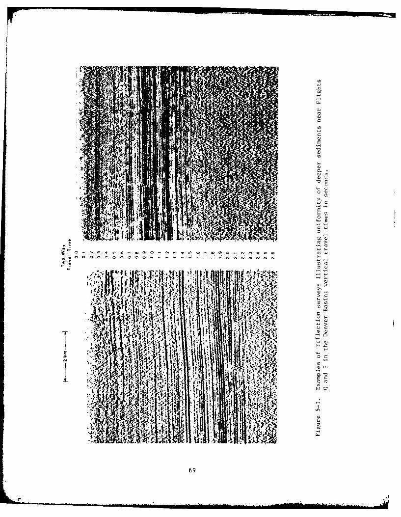
Ln

c - )

Er

0wA.P',

0 0 0 ac 0 0 0 r, rwev C w

IL-

~0 r-

w C,

)OW

q~w ,I -r E

694

i.e. the periods of a free-fixed shear beam. At these maxima the ratio of

surface motion with and without the surface layer is just p2a2/ Pl, the

ratio of characteristic impcdences. As an example consider a simple model of

Denver Basin sediments consisting of a 3 km thick layer with average shear

wavespeed of 1.5 km/sec. Natural periods, T are at 8 sec, 2.67 sec, 1.6 sec,

etc. These periods are within the critical period window of the Wing V system.

Assuming p1 = 2.4 gm/cm 3, P2 = 2.65 gm/cm 3 and 82 = 3.3 km/sec gives an am-

plitude ratio of 2.43. These are representative of the results expected from

a more realistic model of Denver Basin sediments overlying Precambrian base-

ment.

This simple model also provides a quantitative estimate of the effects of

a soft surface layer, specifically the Tertiary deposits. Assuming for example

that the upper 200 meters have a shear wavespeed of 750 m/sec gives natural

periods of T = 1.06 sec, .36 sec, etc. A particularly low shear wavespeed of

500 m/sec gives T = 1.6 sec, .53 sec, etc. Therefore the Tertiary overburden

must have an anomalously low wavespeed to affect missile response at periods

longer than 2 sec. The near surface velocity surveys described in Section 4

give no indication of such low wavespeeds; hence the Tertiary overburden is

apparently not a significant contributor to response in the 2 to 6 second

period window.

The calculational procedure is to construct velocity and density functions

for each of the sedimentary sections given in Table 5-1 and then calculate sur-

face response at each Flight using the Haskell-Thomson approach. The computer

program is available in Herrmann (1978) and described by Haskell (1960),

Haskell (1962). These latter references also show that the surface response

is relatively insensitive to angle of incidence for angles less than 150 from

vertical. Therefore only near vertically incident body waves are considered.

70

Velocity functions are readily constructed from the formation thickness

in Table 5-1 using Faust's fit for P wavespeeds, VP = AZ1 /6 . The constants

determined by Faust for each of the formations, excluding Tertiary, are given

in Section 4. These are increased here by 2% to fit the available well log

data. According to Tosaya's velocity data, Figure 4-3, S wavespeeds are

about half of P wavespeeds for saturated Pierre Shale in the depth range con-

sidered. This corresponds to a Poisson ratio of 1/3. Although some deep well

data in the Wattenberg oil field, north of Denver, Colorado indicate only par-

tial saturation, Matuszczak (1976), it will be assumed here that the Denver

Basin sediments are saturated. Therefore VS is just .5 Vp in the follow-

ing models. Finally, the density function of Gardner for shales, also describedin Section 4, is used to calculate density directly from Vp as p = .32 V1 /4

P P.

The velocity and density functions at Flights P and S in the Goshen Hole area

are shown in Figure 5-2. These are piecewise constant (layered) approxima-

tions of the smooth models for use in the Haskell-Thomson formalism. The up-

per 100 meters representing part of the Tertiary deposits are assigned approxi-

mate properties because 2-6 sec response is insensitive to the variations noted

in Section 4. The Precambrian basement is assigned properties based on gra-

nite wavespeeds at depth given by Press (1966). These are 5750 km/sec, 3324

km/sec and 2.65 gm/cm 3 for P and S wavespeeds and density, respectively.

Amplitude spectra at Flights H, S and P are plotted in Figure 5-3 for S

or SH wave input, and in Figure 5-4 for P wave input, both at normal inci-

dence. Three curves are plotted for each flight; the middle curve is for the

nominal velocity function while the other two are the + 15% bounds, which

bracket the original well log data in Figure 4-1a. Flights H, S and P have

mean depths of 2018 meters, 2820 meters and 3432 meters respectively. In

71

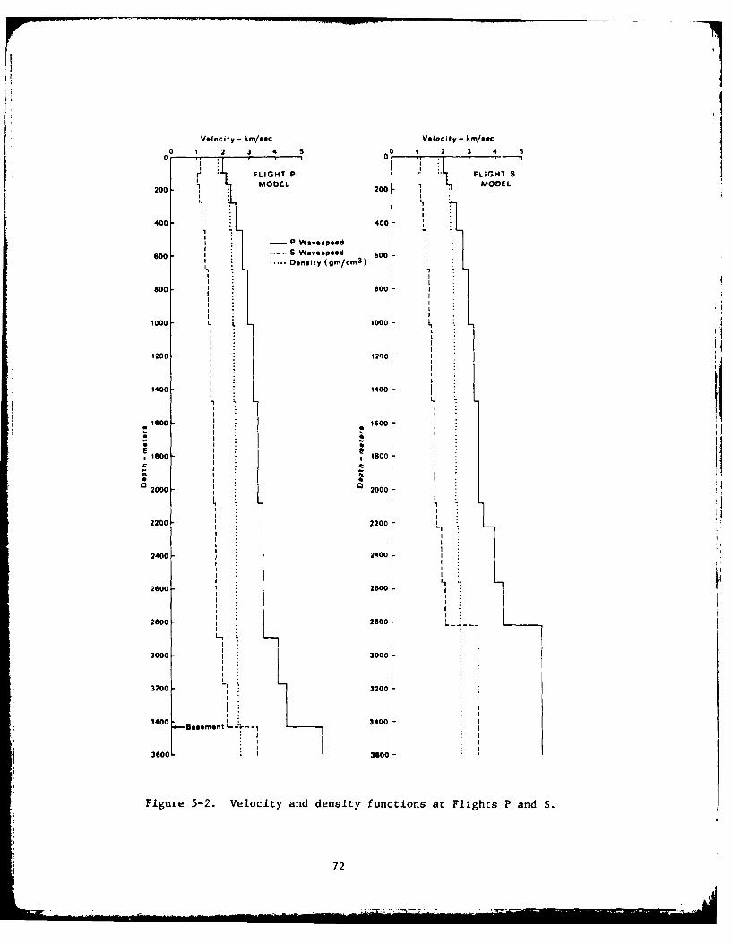
Velocity - km/sec Velocity - km/soc

0 1 2 3 4 5 0 1 2 3 4 5

0 0FLIGHT P FLGH

200MODEL 20MODEL200 ;200I F

400 400

0 Wavespeed 600

I ..... Density (qm/cm3

)

800 800

1000 1000

1200 1200

1400 1400

1600 1600

E "* 1800 1

200 2002000 2000

2200 2200

2400 2400

2800 2600

3000 I3000

3200 3200

3400 1 3400

r Basem nt

--

3600 2800I

3000 200

Figure 5-2. Velocity and density functions at Flights P and S.

72

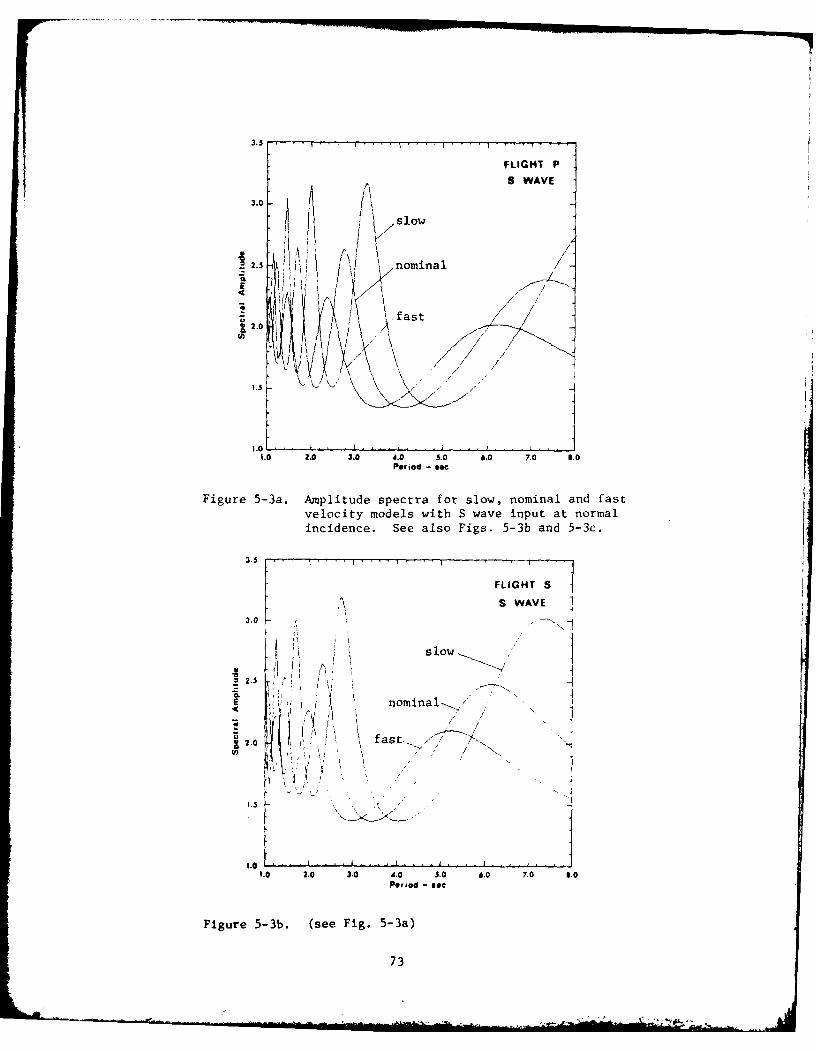
3.5

FLIGHT PS WAVE

3.0 ! s low

2 2. nominal

~fast

1.0

1.0 2.0 3.0 40 50 .0 7.0 6.0

'Figure 5-3a. Amplitude setafor slow, nmnladfsvelocity models with S wave input at normal

incidence. See also Figs. 5-3b and 5-3c.

FLIGHT S

3.0 WV

S2.5

nominal

2.0 Ist- >-

1.0 2.0 3.0 4.0 5.0 6.0 7.0 S.0Period - see

Figure 5-3b. (see Fig. 5-3a)

73

FLIGHT H

3,0 S WAVE

3.0o

2.5 nominal--"

j20 ~ fast---/

1. 0- I I1.0 2.0 3.0 4.0 5.0 6.0 7.0 3.0

Period -see

Figure 5-3c. (see Fig. 5-3a)

3.5

FLIGHT P

P WAVE3.0

-2.5

slowE

nominal/

1L2.0fast/

fL ..1.; 2.0 3.0 4.0 5,0 6.0 7.0 3.0

Period -see

Figure 5-4a. Amplitude spectra for slow, nominal and fastvelocity models with P wave input at normalincidence. See also Figs. 5-4b and 5-4c.

74

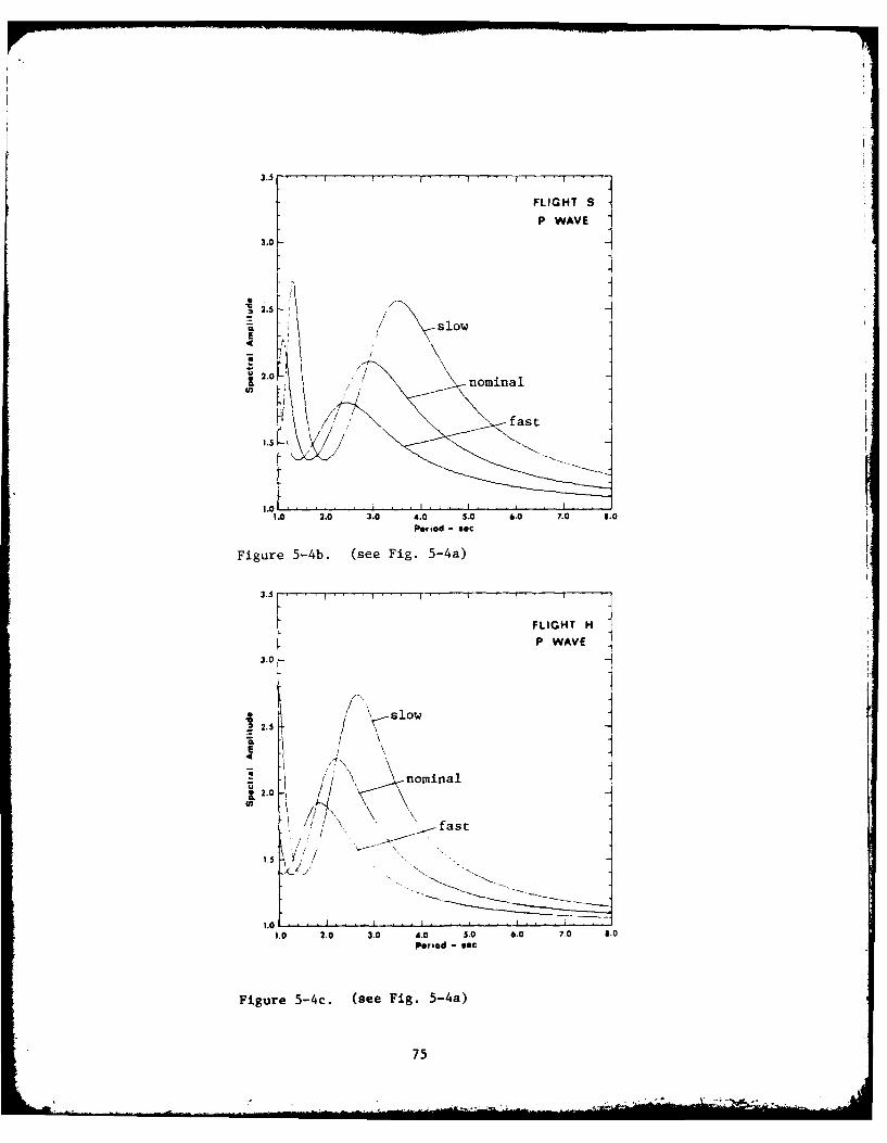
FLIGHT S

P WAVE

3.0

A / slowE '

U

~fast

1.0 2.0 3.0 4.0 5.0 6.0 7.0 8.0

Period - sac

Figure 5-4b. (see Fig. 5-4a)

3S.5 . . . . . . .

FLIGHT H

P WAVE3.0

.3~ ~ \slowS2.5

/1 nominalI2.0 //

/ ~ -fast

to0 2.0 3.0 4.0 5.0 4.0 7.0 3.0Period - sac

Figure 5-4c. (see Fig. 5-4a)

75

general, decreasing the overall velocity function shifts the peak response to

longer periods and higher amplitude, while increasing the velocity function

decreases the peak period and amplitude. The peaks at the longer periods are

the fundamental mode of the layered model and consecutive peaks at shorter

periods are the overtones.

Consider Figure 5-3 showing response to S waves at normal incidence.

The fundamental mode at Flight H ranges from 4 to 5.5 sec and the first over-

tone ranges from 1.5 to 2.2 sec. At Flight S, where bedrock is 0.8 km deeper,

the fundamental is from 5.2 to 7.3 sec and the overtone from 2 to 2.7 sec. At

Flight P, 1.4 km deeper than H, the fundamental range is 6.2 to over 8 sec and

the overtone range is 2.3 to 3.3 sec. Spectral amplitudes of the fundamental and

first overtone generally range from 2 for the + 15% velocity function, to over

3 for the - 15% function. These amplitudes give the increase in surface re-

sponse due to the presence of sediments, i.e. amplitude on an outcrop of base-

ment rock would be unity.

Figure 5-4 shows the surface response to normally incident P waves.

Here the fundamental mode ranges are 1.8 to 2.7 sec. for Flight H, 2.4 to 3.5

sec for S and 2.9 to 4.2 sec for P. The first overtone is less than I sec

for H, reaches 1.4 sec for S and ranges from 1.1 to 1.6 sec for P. Spec-

tral amplitudes of the fundamental and first overtone range from 1.75 to 2.5

for the + 15%, nominal and - 15% velocity functions.

The most notable result of these calculatiors is that the best velocity

function estimate for Denver Basin sedimen' s , fts natural periods in the

range of Wing V missile suspension system natural periods, 2 to 6 seconds.

In particular Flight P, which consistently had a high percentage of seismic

alarms from both earthquakes, rests on sediments which amplify in a window

76

I.t

close to the suspected critical period of the Missile Guidance Set (MGS), 3

to 6 seconds. Comparison of response at P and S shows that periods at Flight

S, although lower than those at P, are still close to the critical MGS win-

dow. However, Flight S in the Goshen Hole had the lowest percentage of seis-

mic alarms. Note also that amplifications at the natural periods are not par-

ticularly high because the mean velocity and density contrasts between sedi-

ment and basement are not great.

As mentioned above, Flight S in the Goshen Hole lowland was relatively

insensitive to the seismic inputs from the Pocatello Valley and St. Elias

earthquakes. Recognizing that absolute estimates of ground motion at any one

flight are subject to the uncertainties of the geophysical model, a better es-

timate of response might be spectral ratios with respect to Flight S. Such

ratios would tend to cancel certain biases of the model. Two examples are

illustrated in Figure 5-5. These show spectra at Flights P and H divided by

the spectrum at Flight S for S wave input to the nominal velocity models.

There are actually three velocity models at each flight, - 15%, nominal,

+ 15%, to be considered in computing these spectral ratios. This gives nine

combinations per flight ratio, or a total of 180 combinations over the twenty

flights for each body wave input (P or S). In what follows all ratios are

with respect to the Flight S (lowland) spectra with either a slow (- 15%),

medium (nominal) or fast (+ 15%) velocity function. For example, spectral

ratios at Flights P and H are shown in Figure 5-6 when Flight S has a fast

model and Flights P and H have slow models. Comparing Figures 5-5 and 5-6

shows that the Flight P ratio has a peak near 3 seconds in both cases.

All possible spectral ratios were calculated for normal incidence of P

and S waves. Rather than show the 360 curves, a less cumbersome approach is

77

2.0 Flight H

is

.;1.0/

CL

0.1.0 2.0 3.0 4.0 5.0 6.0 7.0 8.0

Period -sec

2.0 Flight P

.2N

0.1

1.0 2.0 3.0 4.0 5.0 6.0 7.0 8.0Period -sec

Figure 5-5. Spectral ratios for S wave input with nominalvelocity models (Flights I' and1( H j rt diVidted

by Flight S 78spectrum).

2.0 Flight H

1.0 L , ... . . _-

C LC., 0.

1.0 2.0 3.0 4.0 5.0 6.0 7.0 8.0Period - sec

2.0 Flight P -t

I

- 1.0 ,, / -4

0) V

0.

1.0 2.0 3.0 4.0 5.0 6.0 7.0 8.0Period - sec

Figure 5-6. Spectral ratios for S wave input with a last imdc, I atFlight S and slow model at Flights P and IH (I.lI~htsP and H spectra divided by Flight S spectru1).

79

miA

to indicate the distribution of flights exhibiting spectral ratios greater than

some level within a period window of interest. This is effectively a distribu-

tion of synthetic seismic alarms. They indicate relative amplification with

respect to Flight S, hence susceptibility to higher amplitude motion. They do

not correspond to any absolute motion, specifically that required to trigger a

seismic alarm. Figure 5-7 shows those flights with spectral ratios above

1.35 or 1.5 in the period window of 2.5 to 3.5 sec. The first (a) is for the

nominal velocity model at each flight, the second (b) is for the slow model

and the third (c) is for the fast model. Figure 5-8 shows similar results for

the extreme case of a slow model at all flights except the reference Flight

S which has a fast model; this combination is referred to as slow/fast. This

case exhibits the highest spectral ratios within the more restrictive period

window from 3 to 3.5 seconds. Observe that some of the flights are included

because they amplify P wave input while others amplify S wave input, the

amplification being with respect to the corresponding response at Flight S.

Other period windows exhibit similar patterns, as in Figure 5-9 for a window

from 2 to 2.5 seconds with a nominal/slow combination. To show correlation

with depth to basement, sediment depths are indicated in Figure 5-10.

These results indicate that the relative response between Flight S (low-

land) and most of the other flights (highland) is probably no greater than a

factor of two or so. The spectral ratios are generally higher for S wave

inputs than for P wave inputs. When the velocity functions are on the fast

side of the nominal function the spectral ratios decrease, typically less than

1.3, and the peak periods tend to decrease. If the velocity functions are

higher than those considered here the spectral ratios are fairly flat indicating

no significant differences in the 2 to 6 second window. The synthetic

80

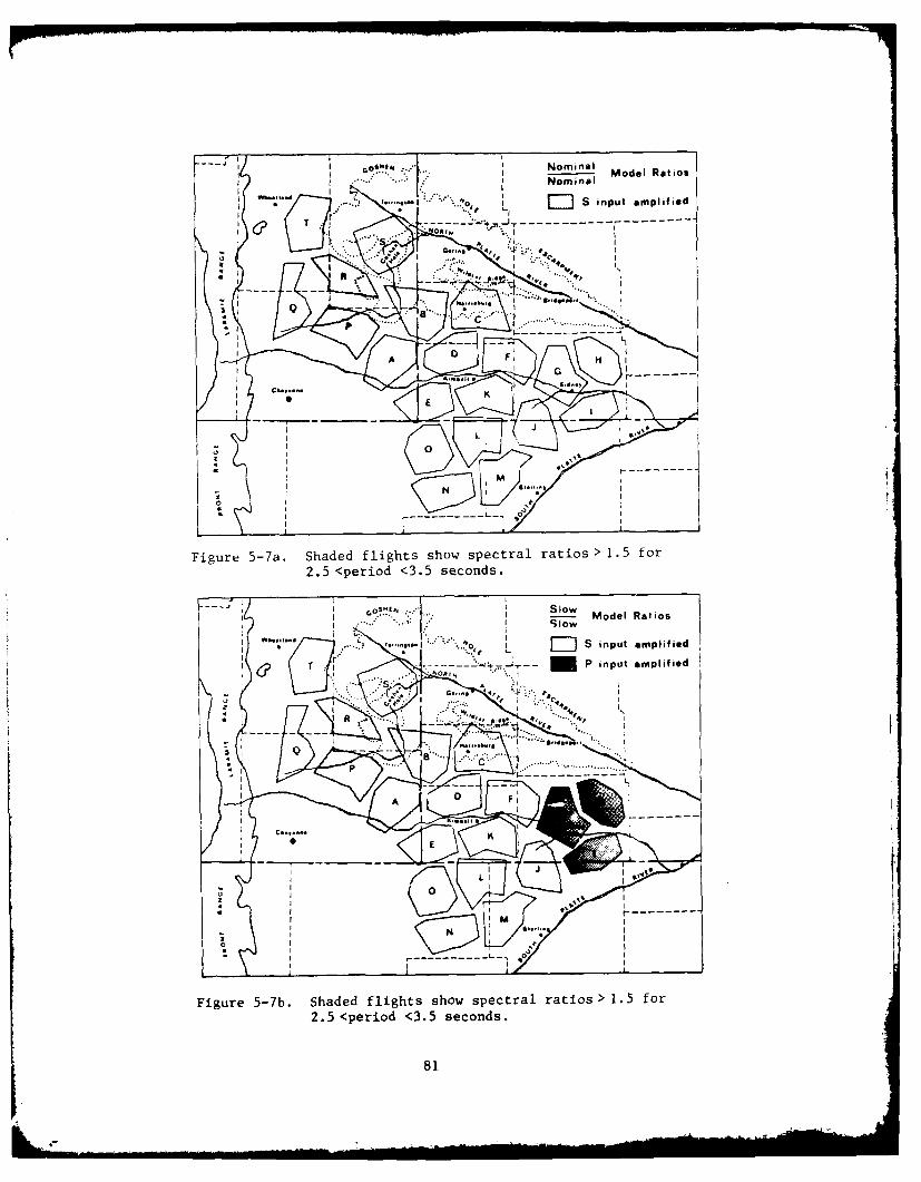
... .. ..* .mfa Model Ratios

..... S nputamplfie

T -- -- -,-, J -- -- -- -- -- -- --

G . II - - - -

Figur .... Khddfihsso peta ais o

2. <perod.<.5...ond

81

I Fast Model Ratios

G O HNP4

...... S l ...... ... ....

-- - Mo- Ratios- --

----------- L i

Figure 5-8. Shaded flights show sectral ratios>1.5 for

3. <~eriod <3.5 seconds.

82o

Moe Ratio

I Nomnina( Model RatiosSlow

S-i-p-t-------ie

Figure -9. Shaed fligts sho spcta rat pios>5for2 <priod <25 seond

SEIEN EPH300350n

P~~ .......................

Figure 5-1. Sapproxiat sdien dpethsl ro Wing fo.

2 <erods<25 scod3

distribution of seismic alarms depends strongly on the location and width of

the chosen period window. Referring to Figure 5-10 showing depth of sediments,

there is a correlation between depth and the synthetic alarm distributions.

Flights P, R and A are the deepest, averaging 3350 meters, and have higher

spectral ratios in the window between 2.5 and 3.5 sec. Flights G, H and I are

the shallowest, averaging 2090 meters and show much lower ratios in this

window.

The spectral ratio peaks and their dependence on velocity functions is

due to the relative periods of fundamental and higher mode resonances at each

flight. Perturbations in the velocity function may shift the fundamental or

overtone into or out of a particular period window. Consequently the flight

where spectral ratios are maximized is still sensitive to biases of the chosen

velocity model, while the range of relative amplitudes is probably less sensi-

tive. Concerning a viable mechanism for the patterns of seismic alarms observed

from the two earthquakes, Figure 1-3, these calculations demonstrate that within

the observed bounds of data scatter about a nominal velocity model there is a

mechanism for selective amplification at some of the flights. The pattern

depends on the type of body wave input, on the critical period window and de-

tails of seismic velocity distributions on a flight by flight basis.

5.2 Additional Wave Propagation Mechanisms

These calculations demonstrate a mechanism for observed patterns of seis-

mic alarms over Wing V due to distant earthquakes. To say whether this is the

actual mechanism or not requires further data on Minuteman III silo mounted

ICBM response to earthquake ground shaking, as well as measurements (rather

than estimates) of velocity structure at the 20 flights. However, the coinci-

dence of sedimentary column resonance periods and estimated Missile Guidance

84

Set natural periods strongly suggest the likelihood of this or a similar

mechanism. These calculations were for body wave input and a natural extension

is to surface waves which are present in the actual seismic input described

in Section 3. For example, relative surface wave response could be found

by assuming the same energy flux for a surface wave mode common to all flights

and calculating ground motion. Amplitude spectra or spectral ratios could

then be determined and presented in much the same manner as was done here

for body wave inputs. A similar procedure was applied by Murphy and Hewlett

(1975) to explain relative seismic response in a preliminary microzonation

of Las Vegas, Nevada.

Other more complex wave propagation phenomena may also contribute to

Wing V anomalies in the Denver Basin. One possibility is focusing of shallow

body waves from the Pocatello Valley event nonuniformly over the Wing V

area due to lateral variations in upper mantle structure under the Rocky

Mountains, Julian (1970). The fact that such focusing could not occur for

the St. Elias event, due to the different travel path, argues against this.

Another possibility is the conversion of incident body waves to surface

waves along the Laramie Range flank. Recent numerical calculations by Harmsen

and Harding (1980) show the Rayleigh wave to be the dominant scattered phase

from a 26.50 flank. The Laramie Range flank is variable and recent COCORP

deep reflection surveys, Allemdinger (1980), have shown it to be a shallow

overthrust as in Figure 2-3c. However, well logs indicate that flank struc-

ture is closer to that shown in Figure 2-3a (see Figure 2-6). Therefore,

estimating the amplitude of scattered Rayleigh waves requires numerical calcu-

lations for various geometries. Scattered amplitudes on the order of 30%

of the incident wave are expected. In any event, the effect of the scattered

85

waves would be greatest near the flank. Because most seismic alarms occurred

farther from the flank and flights on the flank were relatively undisturbed,

this mechanism is of doubtful importance. In addition to mode conversion, the

shallow dip of the flank can also cause energy trapping of body waves, Wojcik

(1979), but to be significant the incidence angle must be quite shallow, which

is not the case for either the Pocatello Valley or St. Elias events.

The possibility of anomalous motions due to variations in crustal struc-

ture has also been considered. In Section 2 it was noted that core rocks of

the Front and Laramie Ranges changed type across the Nash Fork-Mullen Creek

shear zone indicated in the tectonic map, Figure 2-1. The COCORP reflection

survey mentioned above crosses this zone and results indicate a thickening of

the crust by about 25%. Reflections and velocity data north of the shear

zone give a thickness of 38 to 40 km while those south of the zone give 48 to

50 km. Further details of crustal structure under the Laramie and Front Ranges

are given by Prodehl and Pakiser (1980) from refraction surveys conducted by

the U.S. Geological Survey. Predominant body wave periods of their crustal

model are entirely too long to be relevant to this study. Furthermore, the

crustal thickness change across the shear zone would modify the modal distri-

bution of surface wave energy, Alsop (1966), but would not be expected to

amplify or modify Wing V ground response on the scale indicated by alarm distri-

butions.

86

SECTION 6

SUMMARY AND CONCLUSIONS

Wing V, the 90th strategic missile wing near Cheyenne, Wyoming, consists

of 20 flights of Minuteman III ICBMs (10 per flight), distributed over the

tr-state area of Wyoming, Nebraska and Colorado. Due to two recent North

American earthquakes, the Wing experienced significant operational mode

changes (seismic alarms). The earthquakes consisted of a near event, 700 km

west in Pocatello Valley, Idaho (1975), and a more distant event, 3350 km

northwest near St. Elias, Alaska (1979). The Pocatello Valley, Idaho (ML = 6.0)

and the 1979 St. Elias, Alaska (MS = 7.1) earthquakes triggered seismic alarms

in 42% and 46%, respectively, of the Wing V silos. The alarm pattern differed

considerably between the two events. In addition, the tectonic province and

source mechanism as well as incident seismic wave types, amplitudes and durations

differed considerably. The number of alarms indicated some characteristic common

to both events as the causitive factor.

The missile and its suspension system are essentially an inverted pendulum.

Motion is registered at the Missile Guidance Set in the form of disruption counts.

Seismic alarms over Wing V were due to longer period (2 to 6 seconds), lightly

damped (S 1% critical damping) modes of the suspension system. The amplification

factors (i.e. response at resonance) for these modes are high (50-75) but are

only achieved after a large number of input wave cycles. For example, over

three minutes of shaking at a 3.4 second period are required to achieve 90%

of the maximum amplification for the 3.4 second suspension system mode.

Seismograms recorded 200 km south of Wing V on bedrock at Golden, Colorado

* were overdriven by the Pocatello Valley event. However, the more distant

* St. Elias event showed distinct body and aurface wave arrivals. The shortest

periods and longest duration discernable on the record are from body wave

87

phases. Although the bandpass of the Wood-Anderson Seismometer hinders a

direct amplitude comparison, the body waves are generally lower amplitude,

shorter period and longer duration than the surface wave phases (LQ, Lg,

Rg, etc.). Alarm timing and the relative period and duration of body and

surface waves indicated that body waves were the probably cause of the Wing V

alarms.

Wing V is situated over the Denver Basin, a broad, shallow (2 to 3 km)

sedimentary basin, separating the Central/Southern Rocky Mountains to the

west and the Great Plains to the east. Respbnse over the Wing V area is influ-

enced by the interaction of seismic waves with local geologic features, character-

ized by some length scale. If the seismic wavelength is much larger or smaller

than the geologic feature, then little interaction occurs. For the period

window of interest, 2 to 6 seconds, the most significant geologic feature is the

sedimentary cover, in contrast to topography such as escarpments, low velocity

surface layers or crustal depth to Moho.

The predominant sediment in the Denver Basin is cretaceous age Pierre

Shale, with significant deposits of sandstone and limestone. Oil well seismic

velocity logs of the sedimentary columns are well approximated by Faust's fit.

The well log scatter from available data is bounded by ±15% excursions in the

velocity. Therefore, three velocity models were used in the calculations.

The Nominal Model used Faust's values, the Fast Model used 15% higher velocity

and the Slow Model used 15% lower velocity. From well logs and other data,

individual formation thicknesses and total depth under each flight were deter-

mined. Velocity and density functions were found for each of the twenty Wing V

flights using Faust's fit, laboratory data on seismic velocity ratios for

Pierre Shale at depth and density models based on porosity. The sedimentary

88

cover is quite uniform over the Denver Basin. Consequently, a calculational

procedure for a uniform layered halfspace was adequate to investigate the

sediment's effect on body waves.

Near vertical body waves from the distant St. Elias event are incident

on Wing V. The steep incidence angle is due to the high velocity gradient

in the upper crust. Therefore, surface response for P and S body waves at

vertical incidence was examined using a Haskell-Thomson layered halfspace

program. Response at Flight S in the Goshen Hole was used as reference motion

because this lowland flight was relatively insensitive to both earthquakes.

Spectral ratios were developed for each flight by dividing its response by

that at Flight S. Values greater than unity indicate periods where response

is amplified with respect to the lowland flight. All possible combinations of

spectral ratios (with Flight S as the reference) were calculated for P and S

input to the 20 flights with either a slow, nominal or fast velocity model.

Results showed that relative response up to a factor of 2 or so could be

expected. The amplification was due to the relative period and amplitude of

fundamental and higher mode sedimentary column resonances.

The spectral ratios calculated over Wing V with respect to the Flight S

lowland spectrum show that amplification occurs in certain period windows,

which depend on the resonant column periods. These are functions of the

incident wave type (P or S) and the seismic velocity model (fast, nominal or

slow) assumed at each flight. Within the range of assumed velocity models and

period windows of interest, patterns of amplification are seen which correlate

with sediment depth. It was noted that if velocities were all higher than

the nominal measured values, the response became uniform over the wing.

89

In conclusion, within the rather narrow scatter of velocity and depth

data used in the calculations, patterns of amplification with respect to a

reference lowland flight were found for vertically-incident body waves. The

relative response is probably no greater than a factor of 2 or so and the pat-

tern of amplification depends on the period window and body wave type, among

other factors.

The observation that relative amplification between nearby flights can

occur at or near natural periods of the Missile Guidance Set (MGS) suggests

this as the causative factor of Wing V seismic alarm distributions. That is,

the sedimentary column under certain flights amplifies ground response near

natural periods of the MGS. The body wave ground response from distant events

is low amplitude; however, the MGS gain at resonance is sufficiently large to

cause significant MGS motion.

It appears that the Wing V alarm patterns are therefore due to coincidence

of three factors:

1. High gain of 2 to 6 second period missile suspension system

modes.

2. Incident body waves with periods covering the window of the

suspension system modes.

3. Sedimentary column resonance periods close to the suspension

system periods.

Factors 1 and 2 are sufficient to trigger seismic alarms, while factor 3 would

tend to cause anomalous alarm patterns due to relative amplification between

flights.

Prior to the 1979 St. Elias event, explanations for Wing V seismic alarm

patterns centered on a topographic effect due to the Goshen Hole escarpment

90

and/or peculiar earthquake phases from the Pocatello Valley event. However,

the St. Elias seismic alarms suggested that simple body waves were respon-

sible and the calculations reported here support this hypothesis. On this

basis, future North American earthquakes with significant body wave energy

in the period range of 2 to 6 seconds would be expected to trigger seismic

alarms over Wing V in a pattern depending on the depth and velocity of sedi-

mentary cover and the incident body wave type. A quantitative description

of the phenomenon would require: measured (versus inferred) seismic veloci-

ties under a number of flights; the inclusion of material damping, which

is significant for Pierre Shale, in the calculation; and more complete data

on MGS response based on large scale seismic vibration tests.

91

SECTION 7

REFERENCES

Aki, k. and P. G. Richards (1980). Quantitative Seismology, W. H. Freemanand Co.

Allemdinger, R. (1980). Personal communication, Dept. of Geological Sciences,Cornell University.

Alsop, L. E. (1966). Transmission and Reflection of Love Waves at a VerticalDiscontinuity, J. Geophys. Research 71, 3969-3984.

Anderman, G. G. and E. J. Ackman (1963). Structure of the Denver-JulesburgBasin and Surrounding Areas, in Bolyard and Katich (1963).

Arabasz, W. J., W. D. Richens and C. J. Langer (1980). The Pocatello Valley(Idaho-Utah Border) Earthquake Sequence of March-April 1975, Bull. Seism. Soc.

Am. 71, 803-826.

Battis, J. C. (1978). Geophysical Studies for Missile Basing: Seismic RiskStudies in the Western United States, Texas Instruments Inc. report to theAir Force Office of Scientific Research, Bolling AFB.

Battis, J. C. and K. J. Hill (1977). Analysis of Seismicity and Tectonics ofthe Central and Western United States, Texas Instruments Inc. report tothe Air Force Office of Scientific Research, Bolling AFB.

Boatwright, J. (1980). Preliminary Body-Wave Analysis of the St. Elias Earth-

quake of February 28, 1979, Bull. Seism. Soc. Am. 70, 419-436.

Bolt, B. A. (1976). Nuclear Explosions and Earthquakes, W. H. Freeman and Co.

Bolyard, D. W. and P. J. Katich, editors (1963). Guidebook to the Geology ofthe Northern Denver Basin and Adjacent Uplifts, Fourteenth Field Conference,Rocky Mountain Association of Geologists, Denver, Colorado.

Bouchon, M. (1973). Effect of Topography on Surface Motion, Bull. Seism. Soc.Am. 63, 615-632.

Cram, I. H., editor (1971). Future Petroleum Provinces of the United States-Their Geology and Potential, The American Association of Petroleum Geologists,Tulsa, Oklahoma.

Day, S. M., T. C. Bache, T. G. Barker and J. T. Cherry (1978). A Source Modelfor the 1975 Pocatello Valley Earthquake, Systems, Science and Software re-port to the Air Force Geophysics Laboratory, Hanscom AFB, Massachusetts.

Denson, N. M. and M. H. Bergendahl (1961). Middle and Upper Tertiary Rocks ofSoutheastern Wyoming ani Adjoining Areas, U.S. Geological Survey ProfessionalPaper 424-C.

Droullard, E. K. (1963). Tectonics of the Southeast Flank of the HartvilleUplift, Wyoming, in Bolyard and Katich (1963).

92

REFERENCES (CONTINUED)

Ewing, W. M., W. S. Jardetsky and F. Press (1957). Elastic Waves in LayeredMedia, McGraw-Hill Book Co.

Faust, L. Y. (1951). Seismic Velocity as a Function of Depth and GeologicTime, Geophysics 16, 192-206.

Gardner, E.H.F., L. W. Gardner and A. R. Gregory (1974). Formation Velocityand Density-The Diagnostic Basics for Stratigraphic Traps, Geophysics 39,770-780.

Gassmann, F. (1951). Elastic Waves Through a Packing of Spheres, Geophysics16, 673-685.

Geo-Search Corp. (1980). Speculative Seismic Survey, Denver Basin, ChadronArch, Kennedy Basin; Advertising Brochure from Geo-Search Corp. and WesternGeophysical.

Harmsen, S. and S. Harding (1980). Surface Motion Over a Sedimentary Valleyfor Incident Plane P and SV Waves, Bull. Seism. Soc. Am. 71, 655-670.

Harris, D. V. (1963). Geomorphology of Larimer County, Colorado, in Bolyardand Katich (1963).

Haskell, N. A. (1941). The Relation Between Depth, Lithology and SeismicWave Velocity in Tertiary Sandstones and Shales, Geophysics 6, 318-326.

Haskell, N. A. (1960). Crustal Reflections of Plane SH Waves, J. Geophys.Research 65, 4147-4150.

Haskell, N. A. (1962). Crustal Reflections of Plane P and SV Waves,J. Geophys. Research 67, 4751-4767.

Herrmann, R. B., editor (1978). Computer Programs in Earthquake Seismology,1,2, NSF Sponsored, Dept. of Earth and Planetary Sciences, Saint LouisUniversity.

Hume, R. (1980). Personal communication, Navigation Systems Engineering Dept.,TRW, Redondo Beach, California.

Julian, B. R. (1970). Regional Variations in Upper Mantle Structure BeneathNorth America, Ph.D. Thesis, California Institute of Technology.

Keller, G. R., R. B. Smith, L. W. Braile, R. Heaney and D. H. Shurbet (1976).Upper Crustal Structure of the Eastern Basin and Range, Northern ColoradoPlateau, and Middle Rocky Mountains from Rayleigh-Wave Dispersion, Bull.Seism. Soc. Am. 66, 869-876.

King, P. B. (1969). Tectonic Map of North America, U.S. Geological Survey.

King, P. B. (1977). The Evolution of North America, Princeton UniversityPress, Princeton, New Jersey.

93

REFERENCES (CONTINUED)

King, P. B. and H. M. Beikman (1974). Geologic Map of the United States,

U.S. Geological Survey.

Lahr, J. C. (1980). Personal communication, U.S. Geological Survey, MenloPark, California.

Matuszczak, R. A. (1976). Wattenberg Field, Denver Basin, Colorado, inNorth American Oil and Gas Fields, edited by J. Braunstein, The AmericanAssociation of Petroleum Geologists, Tulsa, Oklahoma.

Moore, F. E. (1963). Tertiary Stratigraphy of the High Plains, in Bolyardand Katich (1963).

Murphy, J. R. and R. A. Hewlett (1975). Analysis of Seismic Response in theCity of Las Vegas, Nevada: A Preliminary Microzonation, Bull. Seism. Soc.Am. 65, 1575-1597.

Nafe, J. E. and C. L. Drake (1963). Physical Properties of Marine Sediments,The Sea, 3, Interscience Publishers, 794-815.

Ossing, H. A. and F. A. Crowley (1978). Wing V Ground Motion Study, Air ForceSurveys in Geophysics, No. 401, Air Force Geophysics Laboratory, HanscomAFB, Massachusetts.

Porter and O'Brien, Consulting Engineers (1960). Subsurface Site Investigations,

F. E. Warren Air Force Base, Wyoming Development Area, 1-20.

Press, F. (1966). Seismic Velocities, Handbook of Physical Constants, Geol.Soc. Am., Memoir 97.

Prodehl, C. and L. C. Pakiser (1980). Crustal Structure of the Southern RockyMountains from Seismic Measurements, Bull. Geol. Soc. Am. 91, 147-155.

Rapp, J. R., F. N. Visher and R. T. Littleton (1957). Geology and GroundwaterHydrology of Goshen County, Wyoming, Water Supply Paper #1377, U.S. Geologi-cal Survey.

Richter, C. F. (1958). Elementary Seismology, W. H. Freeman and Co.

Riecker, R. E. (1975). Literature Reconnaissance: Geology of NortheasternColorado, Southeastern Wyoming, and the Nebraska Panhandle, TerrestrialSciences Laboratory, Air Force Cambridge Research Laboratories.

Rodi, W. L., T. C. Bache, J. J. Swanger, T. G. Barker and J. T. Cherry (1979).Synthesis of Regional Ground Motion from Western U.S. Earthquakes, Systems,Science and Software report to the Air Force Geophysics Laboratory, HanscemAFB, Massachusetts.

Smith, F. A. and V. L. Souders (1975). Groundwater Geology of Banner (,oirNebraska, Nebraska Water Supply Paper 39.

Q4

AD-AI07 667 WEIDLINGER ASSOCIATES MENLO PARK CA F/S 8/11

SITE-DEPENDENT GROUND MOTIONS FROM DISTANT EARTHQUAKES. REVISED-,ETC CU)DEC 80 6 L WOJCIK, J ISENBERG, W S DUNBAR F49620-80-C-0009

UNCLASSIFIED R-8065 AFOSR-TR-81-0723 M

EELD

REFERENCES (CONCLUDED)

Smith, R. B., W. J. Arabasz and K. Kilty (1980). Preliminary Geological andGeophysical Data from the Wing V Area, Consultants' Report to WeidlingerAssociates.

Smith, R. B. and M. L. Sbar (1974). Contemporary Tectonics and Seismicityof the Western United States with Emphasis on the Intermountain SeismicBelt, Bull. Geol. Soc. Am., 85, 1205-1218.

Summers, T. S. (1980). Personal comrnnication, Eyring Research Institute,Inc., Provo, Utah.

Telford, W. M., L. P. Geldart, R. E. Sheriff and D. A. Keys (1980). AppliedGeophysics, Cambridge University Press.

Tosaya, C. (1981). Ultrasonic Velocities and Attenuation in Shales: Identi-fication of Shale Lithologies and Delineation of Abnormal Pore Pressures,Stanford Rock Physics Project, 10, Amos Nur, Principal Investigator, 61-101.

Volk, R. W. (1971). Petroleum Potential of Eastern Colorado, Western Nebraska,Southeastern Wyoming and Northeastern New Mexico, in Cram (1971).

Wojcik, G. L. (1979). Resonance Zones on the Surface of a Dipping Layer dueto Plane SH Seismic Input, NSF Grant Report, Weidlinger Associates, MenloPark, California.

95/96

APPENDIX A

NUMERICAL ANALYSIS OF TOPOGRAPHIC SCATTERING EFFECTS

A.1 Introducton

Scattering of waves by the Goshen Hole escarpment was investigated as a

possible contributor to the observed distribution of seismic alarms. As is

discussed above, sources of shaking in the period range 2 to 6 seconds are of

interest in explaining the distribution. Scaling laws suggest that the dimen-

sion of the Goshen Hole escarpment (<200 meters) is too small to interact with

these longer period waves. To support this conclusion, an analysis of shorter

wave periods for which interaction is expected to be maximum was performed.

The present study considers normally incident P and S waves. A two-

dimensional finite element model of a 250 meter escarpment was generated for a

2 to 8 Hz frequency range (.125-.5 second period). The finite element model was

used to develop a Green's function for each type of body wave input. By means of

superposition, a range of input time histories were considered and seismograms

and spectra were generated without further time domain finite element analysis.

In Ref. A-l, Boore et al. used a finite difference model to examine scat-

tering from a vertical and 450 escarpment for a particular time history input.

Earlier, Bouchon, Ref. A-2, considered scattering from ridges and valleys using

a semi-analytical frequency domain analysis. Boore et al. showed the shape of

the escarpment was significant at the relatively high frequencies where scatter-

ing occurred. Bouchon's results indicated that the highland response exceeded

that of the adjacent lowland.

A.2 Numerical Method

The basic numerical tool used in this study was TRANAL, a three-dimensional,

explicit, nonlinear finite element code with constant strain elements in which

A-1

single point integration is used to compute stresses, Ref. A-3. The code was

specialized to treat two-dimensional, linear problems for this study.

The model of the Goshen Hole escarpment is shown in Fig. A-1. Since

the model is assumed to be linear, superposition of elementary solutions

(Green's functions) can be used to obtain the response to complex inputs. The

Green's function best suited to TRANAL is a ramp in velocity. The function is

developed by applying to the bottom boundary of the grid in Fig. A-1 a horizontal

(S wave) or vertical (P wave) velocity-time history which increases linearly

with time. The procedure is illustrated in Fig. A-2. The responses of nodes

on the free surface are stored for future use in response calculations. At sur-

face nodes far from the escarpment, the response is due to the direct wave only

and is equal to the input multiplied by a factor of 2. At surface nodes close

to the escarpment, the response includes both the direct wave and scattered

waves.

By superposition, the responses to a ramp input can be combined to obtain

a wide range of smooth time domain input functions. The function used here is

the Ricker wavelet, Ref. A-4, which is illustrated in Fig. A-3 along with its

spectrum. In the time domain, the wavelet is dispersed as a result of fre-

quency limitations of the finite element grid. However, the distortion appears

negligible when examined in the frequency domain.

A.3 Application to Goshen Hole Escarpment

Seismograms resulting from P wave input are shown in Figs. A-4 and A-5.

These seismograms are observed at highland and lowland stations which are

equally spaced from the edges of the escarpment. The first signal is the input

wavelet, which arrives simultaneously at all lowland points, and soon thereafter

A-2

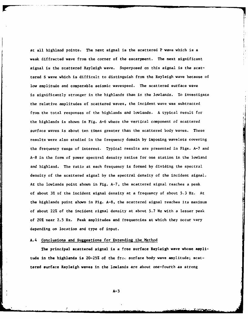
at all highland points. The next signal is the scattered P wave which is a

weak diffracted wave from the corner of the escarpment. The next significant

signal is the scattered Rayleigh wave. Superposed on this signal is the scat-

tered S wave which is difficult to distinguish from the Rayleigh wave because of

low amplitude and comparable seismic wavespeed. The scattered surface wave

is significantly stronger in the highlands than in the lowlands. To investigate

the relative amplitudes of scattered waves, the incident wave was subtracted

from the total responses of the highlands and lowlands. A typical result for

the highlands is shown in Fig. A-6 where the vertical component of scattered

surface waves is about ten times greater than the scattered body waves. These

results were also studied in the frequency domain by imposing wavelets covering

the frequency range of interest. Typical results are presented in Figs. A-7 and

A-8 in the form of power spectral density ratios for one station in the lowland

and highland. The ratio at each frequency is formed by dividing the spectral

density of the scattered signal by the spectral density of the incident signal.

At the lowlands point shown in Fig. A-7, the scattered signal reaches a peak

of about 3% of the incident signal density at a frequency of about 5.3 Hz. At

the highlands point shown in Fig. A-8, the scattered signal reaches its maximum

of about 22% of the incident signal density at about 5.7 Hz with a lesser peak

of 20% near 2.5 Hz. Peak amplitudes and frequencies at which they occur vary

depending on location and type of input.

A.4 Conclusions and Suggestions for Extending the Method

The principal scattered signal is a free surface Rayleigh wave whose ampli-

tude in the highlands is 20-25% of the free surface body wave amplitude; scat-

tered surface Rayleigh waves in the lowlands are about one-fourth as strong

A-3

as in the highlands. Resonances occur at frequencies in the range 4-6 Hz,

which is related to the characteristic dimension of the topography (250 m)

and the wavespeed (c = 1240 m/sec). The diffracted body waves are much$

weaker than the surface waves in the frequency range considered. Since this

numerical model does not consider response in the period range 2-6 sec, where

resonance occurs in the fundamental mode of the MGS, we cannot conclude that

seismic alarms are independent of topography. However, nothing in the results

of these studies suggests that significant interaction would occur between

wavelengths of the order of 2 km (for 1 sec waves) and the escarpment even if

the numerical model were expanded to include such longer period waves.

r;, ent extensions of TRANAL have made it possible to consider a wider

range of frequencies for significantly less computer time (on the order of

250 times faster). These extensions include specialization of the code for

problems of this type and adaptation to vector machines such as the CRAY-1.

A-4

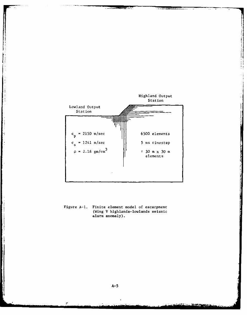
Highland OutputStation

Lowland Output

c = 1241 r/sec 5 ms timestep

P= 2.18 gm/cm 30 m x 30 melements

Figure A-I. Finite element model of escarpment(Wing V highlands-lowlands seismicalarm anomaly).

A-5

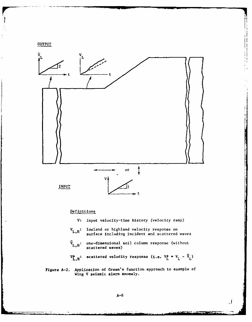
II

OUTPUT

tI

.3 t ,

Sor

V,

INPUT 1

t

Definitions

V: input velocity-time history (velocity ramp)

VL,H: lowland or highland velocity response on

surface including incident and scattered waves

VL,H: one-dimensional soil column response (withoutscattered waves)

V*,: scattered velodity response (i.e. V* - V-VL)L " H L L L

Figure A-2. Application of Green's function approach to example ofWing V seismic alarm anomaly.

A-6 .J

-4.

W o)

Q~L rLI')

* 4.)

Z -- i.Is. 0)M~

,-,- ..

CF ww rL

.. IIx

CD U. ix

L* cu

w

in * . 0)

(A-

z .. jA.lISH301 83MOd

o w

d. 0

W ZW

a: -4

-

I~ 0.

CDV -4 a:Hc

Ix :

InI

A-7 0

-4

K>

K4K0

K-KA

K:

A-8-

-4

k",

(V

C, L

> M

.4

0)

LnV

-3-c

C4C

tV

A--9

J-J

-4

C)

'V

5

'V

'V:5

C)\C) 5-'C)

'V '.3:5I CV

U

C

'V5-'

C

U)

-. 4 F-.4CCU

'-4N 1-I

5-'-~

U) C)'V I-'o-

-4CC'aU)

'a

C.4.3

ItS ~d C~S CN .-4 0

A-1O

STATION L P WAVE

S.76E-0

2.25E-02

1.SOE-02

7.60E-03

6.69 2.96 4.00 6.96 16.06

PRE UECY (HZ)

Figure A-7. Power spectral density ratio (vertical)

scattered spectrumincident spectrum

f or a lowlands point with P-wave input.

A-11

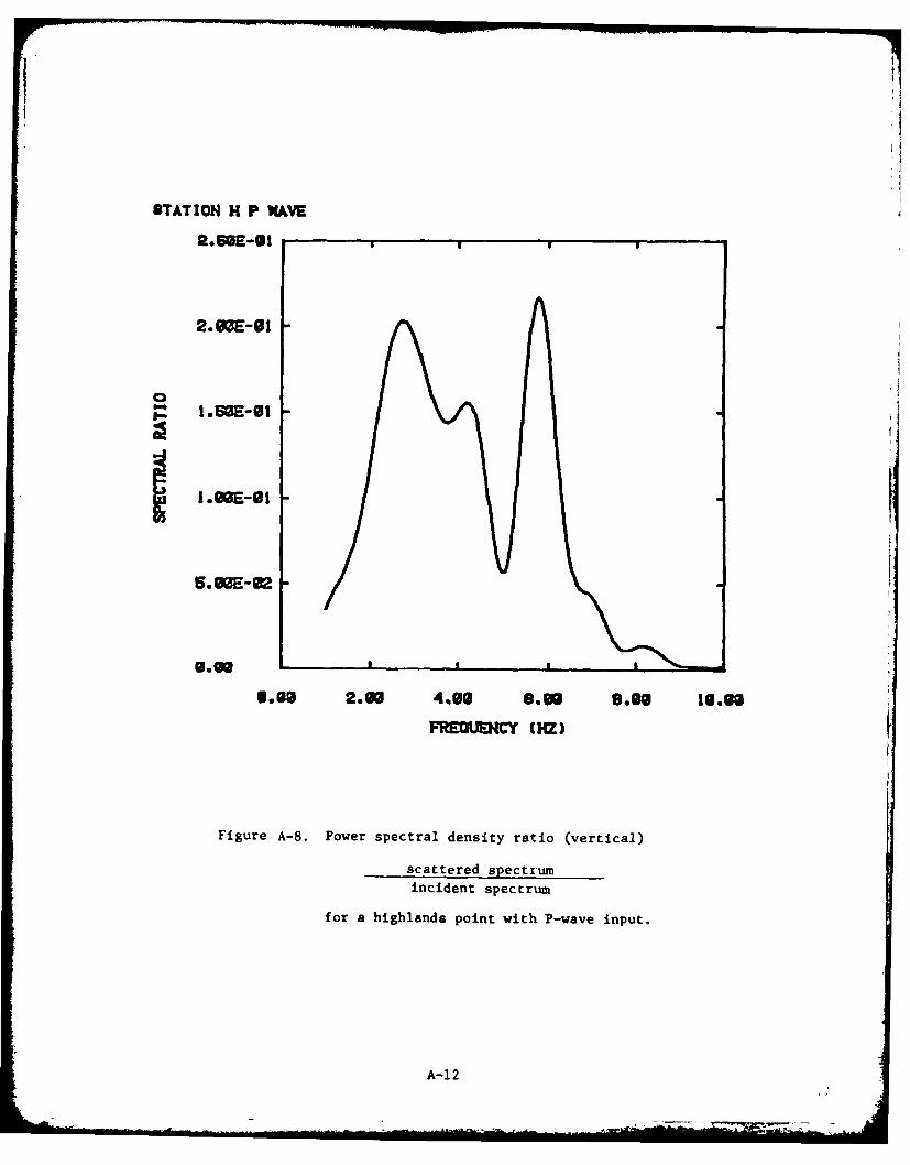
STATION H P XAVE

Q.SME-61

t.WE-8t

5. E-02

5.50 2.90 4.00 8.00 U.S. 16.68

FROUHC CHZ)

Figure A-8. Power spectral density ratio (vertical)

scattered spectrumincident spectrum

f or a highlands point with P-wave input.

A-1 2

!

APPENDIX A

REFERENCES

A-I. Boore, D. M., S. C. Harmsen and S. T. Harding (1981). Wave Scatteringfrom a Step Change in Surface Topography, Bull. Seism. Soc. Am. 63,117-125.

A-2. Bouchon, M. (1973). Effects of Topography on Surface Motion, Bull.Seism. Soc. Am. 63, 615-632.

A-3. Baylor, J. L., J. P. Wright and C. F. Chung (1979). Tranal User'sGuide, Part I (small strain, small displacement), Weidlinger Associates,prepared for Director, Defense Nuclear Agency.

A-4. Ricker, N. (1953). The Forms and Laws of Propagation of Seismic Wavelets,Geophysics 18, 10-40.

A-13