III. PRESSURE FLUCTUATION MEASUREMENT · NASA Grant NGR 37-002-083 ... Tripping was necessary in these tests in order to have a ... ratio of 34:1 is obtained

(NASA-CR-140448) A THEORETICAL AND

Nt-3

FLIGHT TEST STUDY OF PRESSURE

FLUCTUATIONS UNDER A TURBULENT BOUNDARY

LAYER. PART 2: FLIGHT TEST STUDY Unclas

(Texas Univ.) 106 p HC $8.50 CSCL 20D G3/12 555

FINAL REPORT

NASA Grant NGR 37-002-083

Ames Research Center

A THEORETICAL AND FLIGHT TEST STUDY OF

PRESSURE FLUCTUATIONS UNDER A

TURBULENT BOUNDARY LAYER

Project Directors

Ronald L. Panton Richard L. Lowery

Mechanical Engineering Mechanical and Aerospace

The University of Texas Engineering

Austin, Texas Oklahoma State UniversityStillwater, Oklahoma

1,167

'PART TWO J

FLIGHT TEST STUDY f

by

R. L. Panton, R. L. Lowery, and M. M. Reischman

https://ntrs.nasa.gov/search.jsp?R=19740025684 2018-08-20T20:59:59+00:00Z

TABLE OF CONTENTS

I. INTRODUCTION

II. FLOW FIELD CHARACTERISTICS

Glider Description

Inviscid Flow Field

Boundary Layer

III. PRESSURE FLUCTUATION MEASUREMENT

Microphone Selection

Microphone Calibration

IV. RESULTS

Root-Mean-Square Values

Power Spectra

Cross Power Spectra

V. SUMMARY

I. INTRODUCTION

The study of pressure fluctuations under a turbulent

boundary layer was undertaken with the objective of extending

previous work to lower frequencies. Wind tunnel and flight

test measurements are invalid at low frequencies because of

extraneous acoustic noises and free stream turbulence.

A glider was instrumented and used as a test bed to

carry microphones into a smooth flow free of acoustic noise.

Hodgson had previously measured the spectrum of boundary

layer noise on a glider wing. These tests showed a drop off

at low frequencies that could not be reproduced in any other

facility0 Hodgson tripped the boundary layer at 15 percent

chord and tried to pick the zero point in the pressure

gradient curve for his measurement location. This procedure

resulted in measurements made at 50 percent chord.

The measurements reported here were made on the for-

ward fuselage of a glider where the boundary layer could de-

velop naturally and have some length in a zero pressure

gradient before the measurements were made. Two different

sets of measurements were made. First0 measurements with a

single microphone and simultaneous measurement of the

boundary layer profile were made. These tests included

three microphone sizes and both natural and tripped

2

transition. The second set of measurements was a spatial

array of microphones without the boundary layer measurement.

Tripping was necessary in these tests in order to have a

well developed turbulent layer over the entire region.

Prior to the pressure fluctuation tests several

preliminary investigations were conducted. A series of

flights were made to survey the static pressure on the

fuselage forward of the wing and locate a constant pressure

region. Next, a tuft study was conducted to find the flight

speeds at which the flow was aligned with the fuselage.

Finally, the boundary layer was surveyed at several points

for information concerning its velocity profile,

The major results of the complete experimental pro-

gram can be summarized as follows: the boundary layer flow

was found to be typical of a zero pressure gradient layer;

the pressure spectrum was found to drop off at low frequencies,

and the spatial changes in the coherence function were

determined. Convective velocity information was judged to

be incorrect because of phase errors introduced by damaged

microphones.

3

II. FLOW FIELD CHARACTERISTICS

Glider Description

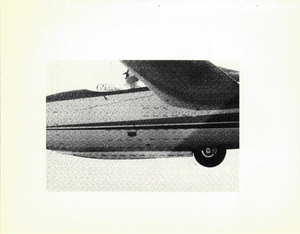
The tests were run on a Schweizer 2-32 sailplane

(Fig. 1). This is an all-metal, two-place0 high-performance

sailplane of rugged construction. Stall speed is around 48

mph and maximum speed 155 mph. At 60 mph the best glide

ratio of 34:1 is obtained. The useful load is 490 pounds.

Measurements were made on the lower portion of the

fuselage just forward of the wing (Fig0 2). In this area

the lower half of the fuselage is a 16 inch radius circular

cylinder for a length of 60 inches. The forward fuselage has

complete cylindrical symmetry tapering down to a 2 inch

radius spherical nose cap. The axis of the nose cap and

forward fuselage section is canted downward at 3.50 with

respect to the axis of the 16 inch cylinder. The nose cap

did not join smoothly to the fuselage so the joint area was

filled and refinished. This left a flat region of 3 or 4

inches around the nose cap joint. In the center of the nose

cap the aircraft total pressure port is located within a

cup-shaped indentation approximately 1 inch in diameter and

1 inch deep. This configuration prevents icing. Air vent

holes are located on each side in the lower quadrant of the

4

nose cap. The vent on the measurement side of the aircraft

was plugged and filled to give a smooth contour, Other

modifications included smoothing the forward fuselage nose-

cap junction.

Inviscid Flow Field

Unpowered aircraft with a fixed weight will have

certain steady state indicated airspeed (or dynamic pressure)

associated with each angle of attack (or lift coefficient).

Therefore the inviscid flow field and pressure distribution

depend only upon the glider angle of attack. From the opera-

tion standpoint picking an indicated airspeed gives a definite

inviscid flow field and pressure distribution for the test

irrespective of altitude. Changing the airspeed not only

changes the Reynolds number, but also gives a slightly

different pressure distribution and flow field. For these

reasons0 most tests were run in the narrow range of airspeeds

55, 60, and 65 mph.

Sailplanes are customarily flown at constant airspeed

by noting the visual position of the horizon on the canopy.

Reference marks on the canopy and the sailplane pitch trim

system allowed the pilot to fly a constant airspeed and

angle of attack without difficulty. A yarn yaw string taped

5

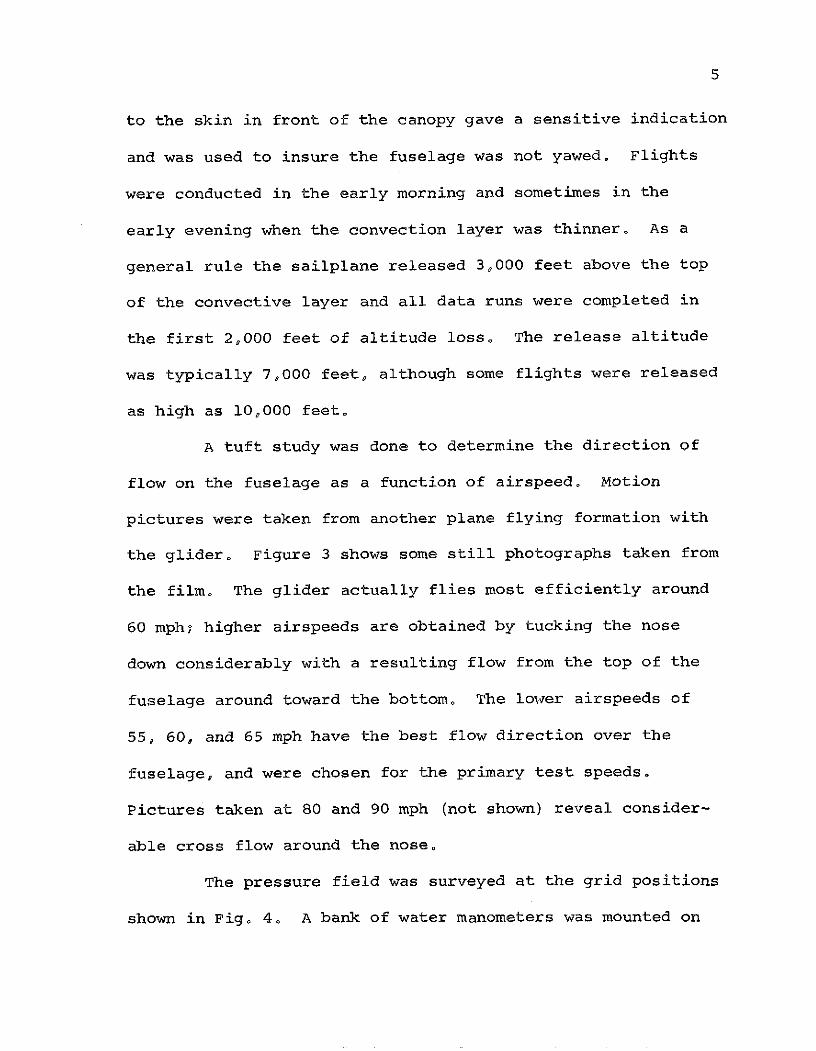
to the skin in front of the canopy gave a sensitive indication

and was used to insure the fuselage was not yawed. Flights

were conducted in the early morning and sometimes in the

early evening when the convection layer was thinner. As a

general rule the sailplane released 3,000 feet above the top

of the convective layer and all data runs were completed in

the first 2,000 feet of altitude loss. The release altitude

was typically 7,000 feet 0 although some flights were released

as high as 100000 feet0

A tuft study was done to determine the direction of

flow on the fuselage as a function of airspeed. Motion

pictures were taken from another plane flying formation with

the glider. Figure 3 shows some still photographs taken from

the film. The glider actually flies most efficiently around

60 mph; higher airspeeds are obtained by tucking the nose

down considerably with a resulting flow from the top of the

fuselage around toward the bottom. The lower airspeeds of

55, 60, and 65 mph have the best flow direction over the

fuselage, and were chosen for the primary test speeds.

Pictures taken at 80 and 90 mph (not shown) reveal consider-

able cross flow around the nose.

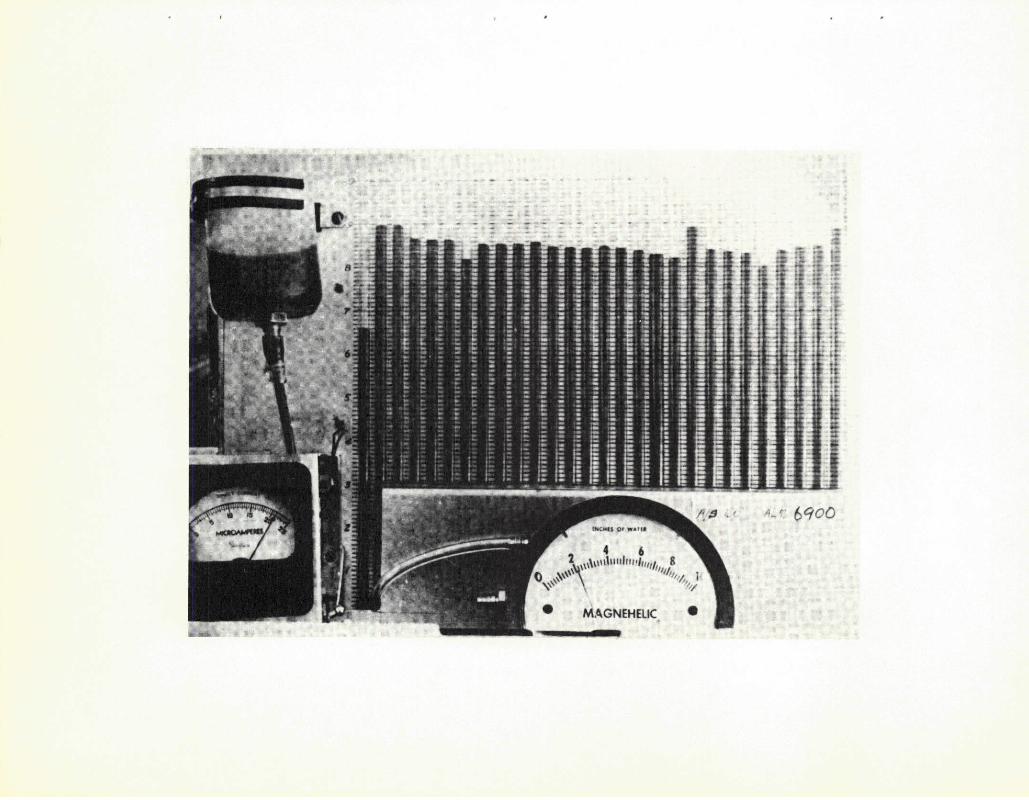
The pressure field was surveyed at the grid positions

shown in Fig0 4. A bank of water manometers was mounted on

6

the back of the pilot's seat and were photographed by the

occupant of the rear seat. A typical photograph is shown

in Fig. 5.

It was not necessary to know the manometer scale or

inclination about the pitch axis. The pressures were

referenced to P and the total pressure P measured; thenO0

C = (P - P )/q is found by dividing P - P column by thep

P - P column. Although the pitch inclination was not0

important0 errors in the roll axis have considerable influ-

ence on the results. A roll error in mounting the manometer

board was measured in the hanger when the wings were level.

From one side of the board to the other, a .1 inch difference

in scale was noted0 and a correction for this effect was

incorporated in the data reduction. Although the difference

between adjacent manometers is small0 the correction accumu-

lates to the order of .05 in C over the length of thep

measurement region. The manometer board gave consistent

results for several different flights0 including one removal

and reinstallation. It is felt that the pilot could fly

with the wings level to within a very small error. A one

degree error in roll is equivalent to six inch error at the

wing tip. Considering reading accuracy and data reduction it

was estimated that an error of ±0.02 in C could occur forp

any point.

'I

The static pressure survey results are given in Figs.

6 through 19. Pressure coefficient as a function of distance

in the flow direction is plotted from an arbitrary origin

43.6 inches aft of the nose (see Fig. 4). The highest row,

A0 is in front of the wing0 and the C plot shows the effectp

of the flow stagnating. A plot for row B shows the same

effect 0 but has one point which is located under the wing at

x = 60 inches. At this point0 the air has accelerated to go

under the wing and the pressure drops. Plots for rows C and

D show similar trends with decreasing influence as one moves

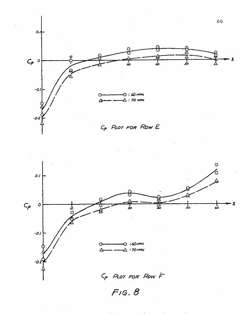
away from the wing0 At the forward stations0 Figs. 8 and 9,

also show the flow recompressing from the low pressure ob-

tained as the flow turns around the nose. The C plot forp

row E shows a region of constant pressure of about 40 inches.

A plot for row F has a slight dip in pressure at about x =

40 followed by a compression as the flow nears the main

landing gear. The dip has been checked0 and is not an error

in data reduction0 but it is somewhat unexpected. It is

within the accuracy of the measurement.

Cross-plots giving the pressure field at a fixed

station are shown in Figs. 12 through 18. The origin for

these graphs was the top row of taps and the Y distance is

measured along the skin (see Fig. 4). Transverse pressure

8

gradients0 except at wing level0 are moderate until one

progresses to column 7 which is under the wing; here both

the wing and wheel effects are evident.

A line slightly above Row Eo 50.7 degrees down from

horizontal on the cylinder0 was selected for the primary

microphone instrumentation. The pressure distribution along

this line and continuing to the nose is shown on Fig. 19.

The region for the measurements was located somewhat lower

than we expected prior to taking the pressure survey.

Mounting brackets which would accept two 2-inch

diameter instrument plugs were attached to the sailplane along

the measurement line. One bracket was located so the aft

hole was 83.5 inches from the nose 0 and the other bracket

located at 60.6 inches from the nose. Figs. 13 and 14 which

show the final microphone arrays0 also give the location of

the instrument plugs.

Boundary Layer

The boundary layer mean velocity profile was found

at two stations along the measuring line; the aft plug of

each bracket. On tests where a single microphone was used0

it was placed at the 80.4 inch station0 and a traversing

pitot tube located at the 83.5 inch station. In order to

9

establish the boundary layer growth0 some additional data

were taken at the 60.6 inch forward bracket location. The

traversing pitot probe was driven with a cam in such a way

that it moved very slowly near the wall. It made one cycle

in about 20 seconds and stroked 2 inches. The static tap

was located in the same instrument plug at a position where

the reading did not change as the pitot traversed in and out.

Position of the pitot was measured electrically and recorded

on tape0 along with the pressure transducer signal. Analysis

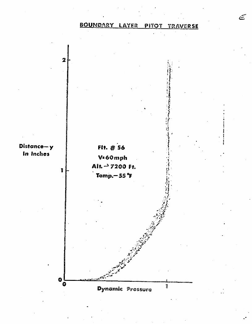
of the boundary layer was done by plotting the profiles of

three consecutive traverse cycles on an x-y plotter as shown

in Fig. 22. An average line was then drawn and points taken

from this line for computer processing.

In analyzing the boundary layer data the method used

in the "1968 AFOSR-IFP-Stanford Conference on Computation of

Turbulent Boundary Layers" was employed. Many previous wind

tunnel experiments have been processed by the same method and

the results are given in the conference proceedings. The

boundary layer is assumed to be one of the profiles from the

"equilibrium" family. The law of the wall plus the law of

the wake is written in the following form:

u= 1 (y ) + C + 2H sin 2 ( Y)u* k v k 2 6

10

where

u = mean velocity

y = distance from wall

u* = friction velocity = (Tw/p)

T = wall shear stressw

p = fluid density

v = kinematic viscosity

K = Von Karmann constant (.41)

C = law of wall constant (5.0)

S= wake parameter

6 = boundary layer thickness

The procedure adopted by the conference and followed by us

was to choose K and C and determine the values of u*, R and

6 by a least squares fit to the data points. The fit ex-

cludes points in the inner 15% and outer 25% of the boundary

layer. The inner points are excluded because of questions

about the accuracy of a pitot tube when the fluctuations

in velocity become a large portion of the mean velocity. The

outer points are excluded because of the known deficiency of

the wake expression to transition properly into the free

stream.

The three parameters u*, 6, and R characterize the

boundary layer, and any other "thickness" or shape parameter

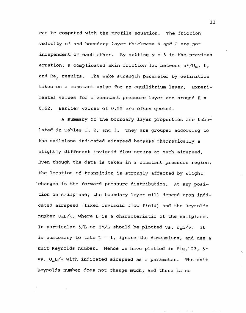
can be computed with the profile equation. The friction

velocity u* and boundary layer thickness 6 and R are not

independent of each other. By setting y = 6 in the previous

equation, a complicated skin friction law between u*/U,, ,

and Re results. The wake strength parameter by definition

takes on a constant value for an equilibrium layer. Experi-

mental values for a constant pressure layer are around a =

0.62. Earlier values of 0.55 are often quoted.

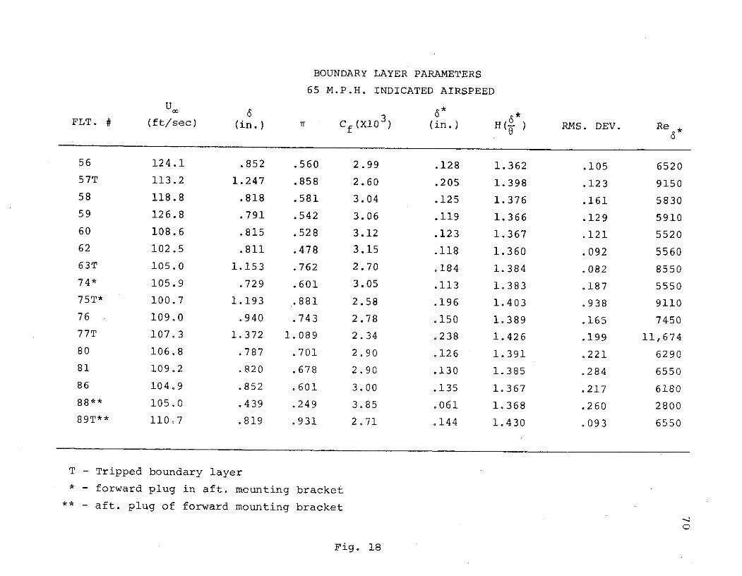
A summary of the boundary layer properties are tabu-

lated in Tables 1, 2, and 3. They are grouped according to

the sailplane indicated airspeed because theoretically a

slightly different inviscid flow occurs at each airspeed.

Even though the data is taken in a constant pressure region,

the location of transition is strongly affected by slight

changes in the forward pressure distribution. At any posi-

tion on sailplane, the boundary layer will depend upon indi-

cated airspeed (fixed inviscid flow field) and the Reynolds

number UL/v, where L is a characteristic of the sailplane.

In particular 6/L or 8*/L should be plotted vs. UcL/v. It

is customary to take L = 1, ignore the dimensions, and use a

unit Reynolds number. Hence we have plotted in Fig. 23, 8*

vs. U L/V with indicated airspeed as a parameter. The unit

Reynolds number does not change much, and there is no

12

discernible trend in 6*. H-igher indicated airspeed, on the

other hand, increased the boundary layer thickness by moving

the transition forward. Flights 76 and 77 are consistently

too high in 8* (also 6 and H) at all airspeeds, and the data

is judged to be erroneous. The reason is unknown.

After the boundary layer has developed, its structure

in nondimensional terms should be like any other zero pressure

gradient layer. Figures 24, 25 and 26 display Cf (Cf =

2u 2/U), 1, and H (H = 6*/0) as functions of Re * Indicated

airspeed should enter these graphs only through Re,*, and not

as a parameter. For comparison, the experimental measurements

of Wieghardt are also plotted. Wieghardt's data was chosen

by the AFOSR-IFP-Stanford Conference as typical of a zero

pressure gradient layer. Wieghardt's data were taken at

various distances along a flat plate in a wind tunnel. The

leading edge of the plate was blunt with a trip wire attached.

Figure 24 gives the skin friction coefficient vs.

Reynolds number. The scatter in the data points gives an

indication of the degree of consistency between flights and

airspeeds. As mentioned previously, the velocity profile

equation employs a skin friction law which could be of the

formC f(1,Re6 *). Wieghardt's data is consistent with the

curve C (f = .62, Re *), except for a small deviation at

13

low Re *. Lower values of H produce a skin friction curve

which is higher. The data points marked "FP" were taken at

the front instrument mounting position at station 60.6. In

the untripped case the forward points are somewhat higher than

Wieghardt's data. Another noticeable trend is that the

tripped data is lower than the untripped experiments.

The trends of the C curves and the associated values

of n are, of course, consistent because of the method of

calculation. When plotting H vs. Re * in Fig. 25 it can be

seen that for the untripped layer, the data are scattered

around 0.5 to 0.6; this is slightly lower than fully developed

value of 0.62, which Wieghardt's data achieves at large

Reynolds numbers. The untripped forward plug points are

around 0.2. There is a well-known tendency for H to drop

off at the beginning of a constant pressure layer. It

appears that the turbulent boundary layer is still young

at the forward position, but has matured by the time it

reaches the aft instrument location. On the other hand, the

tripped boundary layer has higher values of the wake compo-

nent, that is; H = 0.5 to 0.9 and shows no drop-off at the

forward position.

The shape factor is plotted in Fig. 26. Again the

untripped data follows the trend of Wieghardt's data at the

14

aft position, but not at the forward position. The tripped

boundary layer data are somewhat higher, but follow the

proper Reb* trend when the airspeed is constant. There is

a tendency for the tripped points to be further from the

curve as the airspeed increases. Returning to the wake factor

H curves, one can also see a slight trend for R to increase

with higher airspeed. One must conclude that there is an

artifact of the tripping, which increases the wake component

slightly over its nominal value. The amount of the increase

is a weak function of the indicated airspeed. In order to

put this in perspective, the boundary layer velocity profile

data recently published by Wills (4) was processed in a

similar manner. The value of 1 computed was 0.89, which is

larger than the data points reported here at 55 and 60 mph.

In the spatial correlation tests, since the micro-

phones were mounted large distances apart, it is necessary to

account for boundary layer growth. Boundary layer data from

the two mounting positions was interpolated (and extended aft

in one case) by assuming a simple power law growth formula:

n+ln+3

6 = C(x - x )n+30

where n is the exponent in the velocity profile u/U =

( 1/8)/n. An averae value of H = 4 imlies that n is(y/8) .An average value of H = 1.4 implies that n is

15

equal to 5. The constants C and x may be determined at each0

airspeed from the two measurements. The "apparent" origin

of the turbulence, xo , was measured forward of the front

measuring position (station 60.6 inches) and is at least a

qualitative indication of the length of turbulence in front

of the first station.

A/S X untripped C X tripped Co o

55 13.2 in. .00747 39.6 in. .00768

60 15.2 in. .00734 42.4 in. .00795

65 14.8 in. .00804 47.5 in. .00797

The small lengths for the untripped tests agree with the

idea that the E values at the first station were low because

the boundary layer was young, and the wake component not yet

fully established.

To summarize: A region of zero pressure gradient was

located along the lower fuselage, with a length of about 40

inches and a width of perhaps 15 inches; the flow direction

was aligned with the fuselage at the low airspeeds, and tests

were therefore limited to 55, 60 and 65 mph. The untripped

boundary had the mean flow properties of a nominal zero

pressure gradient layer at the aft measuring position, but

had a very small wake component at the forward position;

the tripped layer had nominal mean flow properties at both

16

locations, except for a slightly large wake component and

slightly low C . This component was not so large that the

boundary layer should be considered abnormal.

17

III. PRESSURE FLUCTUATION MEASUREMENT

Microphone Electronics

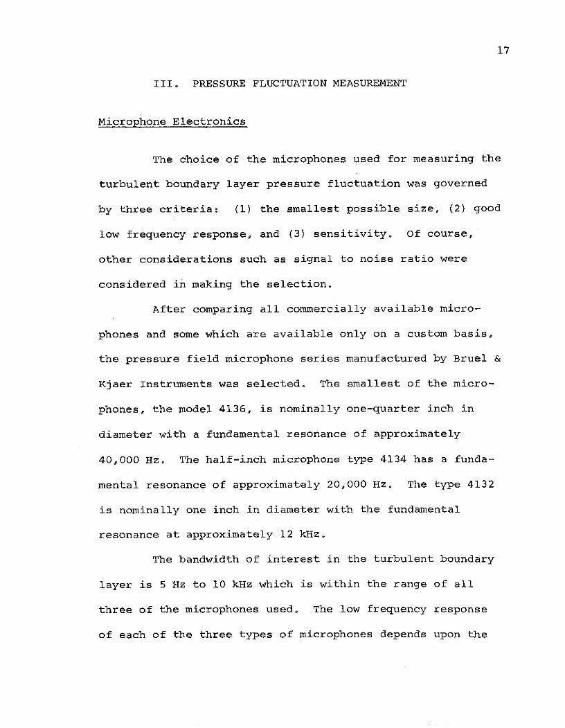
The choice of the microphones used for measuring the

turbulent boundary layer pressure fluctuation was governed

by three criteria: (1) the smallest possible size, (2) good

low frequency response, and (3) sensitivity. Of course,

other considerations such as signal to noise ratio were

considered in making the selection.

After comparing all commercially available micro-

phones and some which are available only on a custom basis,

the pressure field microphone series manufactured by Bruel &

Kjaer Instruments was selected. The smallest of the micro-

phones, the model 4136, is nominally one-quarter inch in

diameter with a fundamental resonance of approximately

40,000 Hz. The half-inch microphone type 4134 has a funda-

mental resonance of approximately 20,000 Hz. The type 4132

is nominally one inch in diameter with the fundamental

resonance at approximately 12 kHz.

The bandwidth of interest in the turbulent boundary

layer is 5 Hz to 10 kHz which is within the range of all

three of the microphones used. The low frequency response

of each of the three types of microphones depends upon the

18

capacitance of the preamplifier used. While several different

versions of electronics are available for this series of

microphones, the Bruel & Kjaer type 2619 preamplifier was

selected since it operates well from a battery powered supply

and has a very high input impedance. The design of the

Bruel & Kjaer condenser microphone is such that the low

frequency response is governed by the capacitance of the

microphone and not the acoustic vent time. For example, the

smallest of the microphones used, the 4136, is designed with

the pressure equilization vent sized so that the -3 db cutoff

point is between .5 and 5 Hz. The typical frequency response

of the type 4136 pressure field microphone operating with the

type 2619 preamplifier is flat between 5 Hz and 10,000 Hz at

random incidence. The pressure response is down 3 db at 3 Hz.

The one-half inch and one inch models display equally good

low frequency response characteristics.

The method of assembly of the Bruel & Kjaer micro-

phone is such that a small shoulder is left at the periphery

of the diaphragm. Otherwise the microphone is sufficiently

flat that it would not disrupt the boundary layer. Since

the shoulder is outside of the active diaphragm area, it is

possible to fill the Champford Annulus with a soft lacquer

to present a flatter surface to the boundary layer. This

19

technique was used on the 1/2 and 1 inch diameter microphones

with no noticeable detriment in performance. The annulus on

the 1/4 inch microphones was small enough to be considered

unimportant.

The one-quarter inch microphone was considered the

primary transducer since the size correction factor would be

less than those of the larger microphones. This microphone,

however, was inferior to the other two models in the areas

of self-noise and sensitivity. However, since the root mean

square levels of the pressure fluctuations at the boundary

layer are on the order of 100 db the relatively high threshold

of the quarter inch microphone was not a problem. However,

the 1/4 inch microphone is extremely fragile and practically

all of them were damaged during the test program.

Since the magnetic tape recorder requires considerably

more voltage than that produced by the type 2619 microphone

pre-amplifier, additional amplification was utilized. A

bank of integrated circuit operational amplifiers was con-

structed which produce the needed gain without a sacrifice

in frequency response. The operational amplifiers used in

the system, which were manufactured by Analog Devices,

proved to be quite stable in gain setting and zero offset.

This type of device was selected for the reason that most

20

conventional wide-band data amplifiers include many additional

features and flexibility which were not required for this

application since most of the tests were made at a single

value of system gain. The operational amplifiers also have

the advantage of requiring very low battery drain, permitting

a large number to be incorporated in the aircraft.

The microphone signals and other flight data were

recorded on a Leach Corporation model 3200 tape recorder.

This recorder operates on 28 volts DC. Twelve channels

recorded in the FM mode and two channels were operated in the

direct mode. Several flight variables, pressures and tempera-

ture, were multiplexed on the direct channels through voltage

controlled oscillators. Six minutes of recording were avail-

able when the recorder was operated at 30 ips.

The main power supply was a set of motorcycle batteries.

The batteries, tape recorder, and assorted electronic devices

were mounted into a module. The module was then secured by

the seat belt attachments into the second seat; immediately

behind the pilot. The pilot could control the recorder,

power supplies, and traversing motor through switches on his

panel.

21

Microphone Calibration

A number of microphone calibration schemes were

tested before the final version was put into effect. Ordi-

narily a microphone is tested at the factory and supplied to

the purchaser with a calibration curve traceable to the

National Bureau of Standards. However, the microphone

diaphragms were exposed to flying debris during the takeoff

and landing of the aircraft and were also subjected to shock

and vibration and various forces and moments during their

installation and removal from the craft. In several instances

the sensitivities of the microphones were noticeably changed

after a period of use. Therefore, the final calibration

procedure involved the use of a piston phone type device

applied over the face of the microphone when mounted in the

aircraft.

The piston phone consists of a small electrodynamic

loudspeaker mounted in a plastic tube approximately twelve

inches long. Neither end of this tube is tightly sealed and

the end applied to the fuselage of the aircraft is equipped

with a soft rubber gasket which was designed to exclude

exterior noises during the calibration process. The seal is

porous and permits air to leak out readily to prevent damage

to the diaphragm when applying the piston phone. The device

22

was calibrated with a standard precision soundlevel meter

which in turn was calibrated with a commercial piston phone

taking into account barometric variations.

A frequency of 500 Hz was selected for the test

frequency since the piston phone was relatively insensitive

to frequency changes. At that point the application of 31

millivolts rms to the loudspeaker of the piston phone pro-

duced a pressure field of 100 db relative to .0002 p bar.

Output was measured at the tape recorder input with the

recorder operating. While earlier tests were made by driving

the transducer with a variable frequency oscillator, the final

test procedure incorporated the use of a power amplifier

having an output impedance of 8 ohms. If the piston phone

is not driven by low impedance source, the minute changes in

electromechanical impedance due to variations in clamping

pressure at the foam rubber seal make the stabilization of

the sound pressure level difficult. When the device is

driven by a small power amplifier the sound pressure level

remains unchanged even if the seal of the tube is lifted

away from the surface a fraction of an inch. This method

of testing proved to be reproducible and in subsequent tests

the sensitivity of the device proved to be quite constant

for over a long period of time and at different temperatures.

23

In addition to the "100 db" test, the rms of the re-

corded signals were measured immediately after each flight.

The rms pressure is closely a function of dynamic pressure

and so varies only with indicated airspeed. Tables which

present the history of each microphone are given in Tables

4 through 13. These histories are during the spatial corre-

lation flight program. Numbers in the same vertical column

can be compared directly. Any number which deviates more than

about ±5% from the average has been underlined.

The half-inch microphones were very consistent except

for number three. The difficulties with this microphone in

the early flights was traced to a bad pre-amplifier. Replac-

ing this amplifier occurred after flight 92, and good results

were obtained thereafter. Of the six remaining underlined

numbers, half occurred on the 65 mph run in flight 96. It

appears that the airspeed was low on this run.

The quarter-inch microphones proved to be easily

damaged. Sometimes the damage was progressive and sometimes

it was traumatic. With use the diaphragms became dull and

showed small pits as if they were bombarded with dust.

Half-inch diaphragms had a similar appearance without any

change in performance. When a microphone gave a bad

calibration one could usually detect a striated scrape mark,

24

a rough mark or several wrinkles somewhere on the active

surface. Microphones with this type of damage usually

showed an increased sensitivity0 operating as if the dia-

phragm was too loose.

Another type of damage was a loose cap. The B&K

microphone is constructed by welding the diaphragm to an

internally threaded cylinder to form a cap. The cap is then

screwed to the base electrode until the diaphragm touches a

support ring. Further screwing stretches the diaphragm to

its proper tension. There is no positive locking of the cap

and in two instances caps were found in a loosened condition.

Damage of this type undoubtedly occurred during ground han-

dling, installation, or removal. When a loose cap is

retightened0 perhaps inadvertantly during installation, it

may be too tight resulting in a decrease in sensitivity.

The histories of quarter-inch microphones show that

only numbers 1 and 3 gave consistent results throughout the

program. Microphone number 5 had only two runs which were

out of the ±5% tolerance but the results tend to get pro-

gressively higher. On flights 95 and 96 microphones 2, 4,

and 6 are probably damaged and 4 and 6 were not flush with

aircraft skin. Excluding the bad microphones of flights 95

and 96, there are 13 out-of-tolerance data points and nine

25

of these occur on 65 mph tripped experiments. This would

seem a significant trend; however, there is no apparent

reason. Measurements of the frequency response of the damaged

microphones were attempted after the flight test program.

Electrostatic actuator tests showed that all microphones

sensitivities would not drop more than 2 db until the fre-

quency was lower than 20 cycles. The response curves were

flat out to 10 kHz on the high end. It is not possible to

conclude that the frequency response of the damaged micro-

phones was unchanged because of the artificial nature of the

electrostatic actuator test. In the test a polarization

voltage of 800 volts is applied between the actuator and the

diaphragm. This pulls the diaphragm away from its normal

position. Ordinarily the correction for this effect is

negligible; .however, if the diaphragm has wrinkles, the

polarization voltage might stretch them out and give an

invalid frequency response curve. Attempts to run tests

without the polarization voltage give signals that were too

weak to measure.

Commercial Piston phone tests were also conducted and

the frequency varied from 25 Hz to 500 Hz. These tests also

gave a flat frequency response dropping off only at the low

frequencies. The 2 db down point was usually around 50 Hz.

26

It was unfortunate that it was not possible to obtain high

frequency data with this method.

Tape Recorder Flutter

Flutter from mechanical transport of the tape had a

large component at about 10 Hz. A typical spectrum analysis

of a flutter signal is shown in Fig. 27. Fig. 27 is an

analysis of a recording made while shortening the input so

that only the FM carrier center frequency is recorded. At

one point in the program the recorder representative was

called out to replace some of bearings and adjust the tape

transport mechanisms. In the last stages of the experimental

program the recorder had periods of several seconds where

grinding noise couid be heard. After the program was com-

pleted trouble with the recorder continued and it was finally

sent back to the factory for a complete overhaul. The flutter

signal of Fig. 27 was made after the overhaul and represents

a recorder operating at .015 volts rms which is close to the

flutter magnitudes measured during the test program. Tape

recorder flutter was suspected of contributing to the measured

pressure spectra. Below 50 Hz, however, the level of the

flutter spectrum is too low to allow a significant contribu-

tion.

27

Data Reduction

The tapes were processed by the Ames Research Center

Hybrid Computer facility. The analysis is essentially an

analog processing from a 50 sec tape loop. The filter band-

widths used over the various ranges were:

RANGE BANDWIDTH

5-25 Hz 1 Hz

25-120 Hz 5 Hz

120-500 Hz 20 Hz

500-2400 Hz 100 Hz

2400-5000 Hz 200 Hz

500-10,000 Hz 400 Hz

The data on the first sequence of flights were transcribed

from the flight recorder to a new tape which was forwarded

to Ames. Data for flights 62 and later flights were process-

ed at Ames using the original tape on which the data were

recorded.

Spectra for flights 56 through 59 (files 3924 through

3935) were processed with nominal values of microphone sen-

sitivities and boundary layer parameters. Correction factors

for the actual values are listed in Table 15.

Processing of flights 62 and later flights was done

during one period of time. The first files in this series

28

are invalid (Files 4517, 18 and 19). Subsequent files have

an amplifier correction. For some unknown reason the Ames

tape recorder used in the Hybrid system could not amplify

properly a calibration tape made on the Leach 3200 flight

recorder. The issue was resolved by playing the tapes with

a reproduce amplifier gain of 0.75. A compensating gain

correction was then made in the digital computer processing

so the spectra have the proper gain factor0 and the values

for C integrated from PSD are thus correct. The rms valuesP

read from a meter on the tape loop, called C loop0 must be

divided by .75 to correct for the amplifier gain.

Beginning with files 4520 the Ames tape recorder was

played at 60 ips whereas the data was recorded at 30 ips.

This gives better bandwidths at the low frequencies. It

also causes a displacement of the PSD spectra. Doubling the

speed has the effect of moving the spectra to double the

frequency and reduces the magnitude by a factor of 2. Thus

the spectra in files 4520 through 4563 should be increased

in magnitude and reduced in frequency by a factor of two.

Because of the frequency shift the computer applied the wrong

Corcos corrections and all data with this correction are

incorrect.

29

IV. RESULTS

Two sets of experiments were conducted; single point

measurements and array measurements. In the single point

measurements a single microphone was mounted in the instrument

plug at station 80 (see Fig. 20). The boundary layer travers-

ing probe was placed about 3 inches downstream in the adjacent

instrument plug. The purpose of these tests was to determine

the pressure spectrum while simultaneously measuring the

boundary layer properties. Three different microphone sizes

were used with both tripped and untripped boundary layers.

Spatial correlations were measured with two different

configurations of ten microphones. Boundary layer measure-

ments were not taken simultaneously in these tests. The

boundary layer was tripped to minimize growth effects and

have a well-established layer throughout the region. Array

number one has the microphones clustered at the aft instru-

ment bracket as shown in Fig. 20, Array number two, shown

in Fig. 21, has the microphones clustered at the forward

location.

Root-Mean-Square Values

Three different root mean square values are tabulated

2in Table 14 as C = vp / qo The first, CpT was measured

px D

30

immediately after the flight with a Ballantine True RMS

meter. The second, C ,pi is the numerical integration of the

power spectral density curve. It is an indicator to check

the PSD computation. The third, Cp, is the meter measure-

ment made on the tape loop during the data reduction. It is

considered the most accurate.

Some files need a correction applied to CpL . When

the original tapes were played at Ames to form the tape loop,

the reproduce amplifier was set at a gain of 0.75. This was

set up using a calibration tape made on the Leach flight

recorder. When the spectrum was processed a compensating

change in the microphone sensitivity figure was made. How-

ever, the tape loop rms values were not corrected and all CL

values on files numbered 4520 and higher need to be divided

by 0.75.

Experimental measurements of the rms pressure signal

are frequently nondimensionalized by the dynamic pressure

since it is easily measured. Since many of the turbulence

properties scale with the wall shear stress many workers feel

that it should be used to give a quantity which would be more

2independent of the Reynolds number; that is C px/C = Vp /Tw.px f w

The shear stress coefficient C levels out at the higher

Reynolds numbers, c.f. Fig. 24, and then the distinction

31

is not too important. Our tests were run at small or moderate

Reynolds numbers and it is possible to investigate the merits

of using q or T to scale the data.

On a given flight, the three consecutive runs at

different airspeeds offers a set of data taken with the same

microphone and simultaneously recorded boundary layer informa-

tion while the Reynolds number changes. Fig. 29 gives data

for C taken with three different microphone sizes. FlightpL

58 is not plotted since this microphone had a loose cap and

the calibration is uncertain. There is a general downward

trend in C as the airspeed (or Reynolds number) is increased.pL

One might suspect that this is an effect of microphone size;

however, this is not true. As the airspeed increases the

transition moves forward and makes the boundary layer thicker

at the measuring station. This causes d/b* to decrease which

means one should measure more of the actual rms. Due to

this effect the curve would increase slightly with airspeed.

The companion graph on Fig. 30 gives the rms non-

dimensionalized by the shear stress (CpL/C ). There is no

apparent trend of these curves with airspeed and it appears

that r gives a slightly better correlation.

Because the microphone size parameter d/6* causes a

great influence on the data it is instructive to plot CpL

32

vs. d/8* as in Fig. 31. In addition to the data plotted pre-

viously all of the other single point and array experiments

taken at 60 mph are shown. There is considerable scatter,

-3however, the data trend is toward C = 5-10 , a value often

P

though of as the lowest level for incompressible flow. The

corresponding plot for CpL/C f is also shown in Fig. 32. The

data show slightly less scatter, especially for runs on the

same flight, and trend toward a value of -l.9. Most other

experiments yield a value a little above 2. The evidence that

CpL/C gives a better correlation than C is not overwhelming;pL f p

however, it will be supported by the same trends in the

power spectra.

Power Spectra

The power spectra as they were plotted at Ames usually

have been processed with rough estimates of the boundary layer

parameters and need to have multiplicative scaling corrections

applied. In some cases the processing procedures caused

further scaling changes. The final scaling changes have

been tabulated in Table 15.

The processing was done in two batches; flights 56,

57, 58, 59 and flights 62, 63, 80, 81, 92, 93, 95, 96. The

first batch has to be corrected for slightly inaccurate

33

values of velocity V, dynamic pressure Q, and length parameter

L. The second batch need corrections for L and for tape

speed. The original data was taken at a tape speed of 30

inches per second. The same tapes were taken to Ames and

processed at 60 ips. This causes the spectrum to shift to

higher frequencies by a factor of two and to decrease in

magnitude by a factor of two. The integral of the spectrum

is unchanged.

The power spectra will be given in two sets of

coordinates, GV/Q2 6* as a function of F6*/V and GV/T2 6 as a

function of F6/V. The integral of the spectrum in the first

set of coordinates is C2 whereas it is (C /C )2 in thepIpi pI f

second set.

The spectra for three different indicated airspeeds

(data taken on one flight in each instance) are shown in the

next four figures. Figure 33 gives data taken with a 1/4

inch diameter microphone, Fig. 34 the 1/2" microphone, Fig.

35 the 1" microphone, and Fig. 36 the 1/2" microphone with a

tripped boundary layer. The spectra all show some irregu-

larity at low frequencies, rise fairly smoothly to a peak

and then fall off as the microphone size becomes comparable

with the eddy size. The fall off at low frequencies is

definitely verified.

34

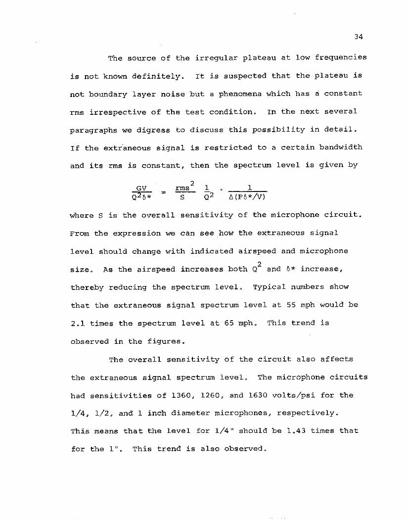
The source of the irregular plateau at low frequencies

is not known definitely. It is suspected that the plateau is

not boundary layer noise but a phenomena which has a constant

rms irrespective of the test condition. In the next several

paragraphs we digress to discuss this possibility in detail.

If the extraneous signal is restricted to a certain bandwidth

and its rms is constant, then the spectrum level is given by

2GV rms 1 o 1Q26* -S Q2 A(F5*/V)

where S is the overall sensitivity of the microphone circuit.

From the expression we can see how the extraneous signal

level should change with indicated airspeed and microphone

size. As the airspeed increases both Q2 and 8* increase,

thereby reducing the spectrum level. Typical numbers show

that the extraneous signal spectrum level at 55 mph would be

2.1 times the spectrum level at 65 mph. This trend is

observed in the figures.

The overall sensitivity of the circuit also affects

the extraneous signal spectrum level. The microphone circuits

had sensitivities of 1360, 1260, and 1630 volts/psi for the

1/4, 1/2, and 1 inch diameter microphones, respectively.

This means that the level for 1/4" should be 1.43 times that

for the 1". This trend is also observed,

35

Another difference should be observed for the tripped

vs. untripped layer at the same airspeed. The change in 8*

should cause the tripped extraneous signal level to be

approximately .7 of the untripped level. There is also an

equivalent shift in the frequency parameter F6*/V. This

trend is observed in Figs. 36 and 37.

The irregularity in the low frequency spectra makes

it hard to definitely conclude that the plateau is an instru-

mentation problem. If it is actually associated with the

turbulent boundary layer one would expect it is not to usual

turbulence-meanshear interaction but another phenomena.

Now we return to the effect of airspeed on the PSD's

as shown in Figs. 33 through 36. The boundary layers for the

three different airspeeds were all typical of a zero pressure

gradient layer. In general we can view the different air-

speeds as simply changes in the boundary layer Reynolds num-

ber, despite the fact that the tuft studies of flow direction

show that the 65 mph run has a small crossflow component.

The rising portion of the spectra and the peak region

are valid measurements. The spectra tend to drop with in-

creasing airspeed when Q and 6* are used to nondimensionalize

the data. The use of T and 6 gives a better correlation on

all four figures. This is consistent with the previous

36

conclusion that CpL /Cf gives a better correlation than CpL.pL f pL

The high frequency roll off should occur at different places

according to the microphone size correction. This changes

very little with airspeed but the lower airspeed should roll

off slightly sooner.

Tripped and untripped data are compared for the 1/4"

and 1/2" microphones in Figs. 37 and 38. The 1/4" data do

not have the right trend at high frequencies. Tripping the

boundary layer thickens 6* by about 50%. This will give a

smaller d/8* and thus a more favorable microphone size

correction, which in turn makes the tripped data to roll off

more slowly. The curves would have this trend if they could

be moved relative to one another. An error in 6* or V would

cause a spectrum to slide along a 450 line from upper left

to lower right. Such an error is suspected. One should

also note that the recorder flutter level is lower for the

tripped data as anticipated.

The 1/2" microphone curves on Fig. 38 give a much

more satisfying comparison. The curves have the expected

trends in every respect in the Q, 6* coordinates, but move

apart when the T and 6 are used as nondimensionalizing para-

meters. This is just opposite of what was found when the

Reynolds number was varied by changes in the airspeed. When

37

one reviews the values of the friction coefficient, which

essentially causes the curves to separate, one finds that

the tripped data is somewhat low and the untripped data

slightly high compared to Wieghardt's data at the same

Reynolds number.

Cf measured C Wieghardt-3 -3

Tripped 2.78*-10 2.86-10-3 -3

Untripped 3.25*10 3.20-10

Ratio squared 1.36 1.25

Since C is involved in transferring data from the top graphf

to the bottom graph, the separation would be slightly less if

we used Wieghardt's data rather than our own.

Another thing that should be pointed out is that the

curves probably should not lie exactly together on either

graph. The boundary layer data for the tripped and untripped

layers showed distinct differences in the wake component n.

Since the shear stress vs. Reynolds number curve is different

for each value of H and since the spectrum should also be

different for each value of H, we should not expect exactly

the same spectra. It is not possible to conclude from the

data at hand exactly what the differences should be, although

a higher 1 gives a higher spectrum, and the data shown here

is in qualitative agreement with this fact.

38

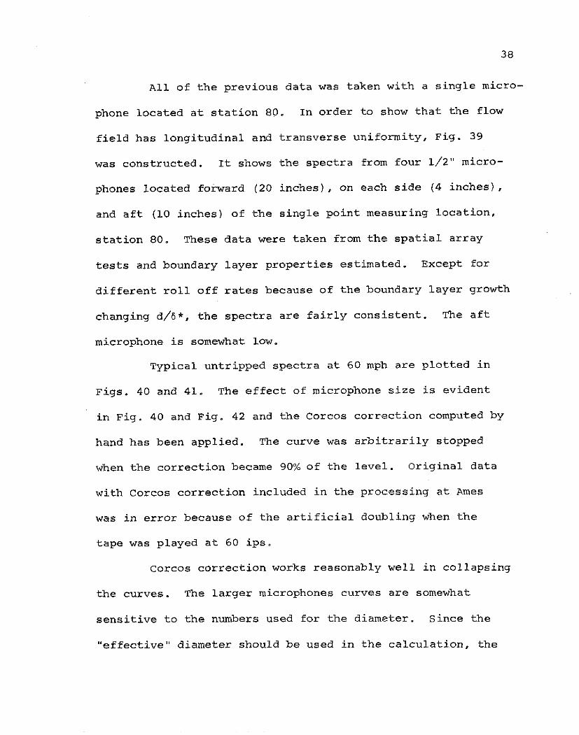
All of the previous data was taken with a single micro-

phone located at station 80. In order to show that the flow

field has longitudinal and transverse uniformity, Fig. 39

was constructed. It shows the spectra from four 1/2" micro-

phones located forward (20 inches), on each side (4 inches),

and aft (10 inches) of the single point measuring location,

station 80. These data were taken from the spatial array

tests and boundary layer properties estimated. Except for

different roll off rates because of the boundary layer growth

changing d/6*, the spectra are fairly consistent. The aft

microphone is somewhat low.

Typical untripped spectra at 60 mph are plotted in

Figs. 40 and 41. The effect of microphone size is evident

in Fig. 40 and Fig. 42 and the Corcos correction computed by

hand has been applied. The curve was arbitrarily stopped

when the correction became 90% of the level. Original data

with Corcos correction included in the processing at Ames

was in error because of the artificial doubling when the

tape was played at 60 ipso

Corcos correction works reasonably well in collapsing

the curves. The larger microphones curves are somewhat

sensitive to the numbers used for the diameter. Since the

"effective" diameter should be used in the calculation, the

39

correction is somewhat uncertain for large microphones. These

spectra on these curves are probably the most accurate of any

of the current measurements and the peak and high frequency

end are in agreement with previous experimenters.

The spectra for the spatial correlations were not

nearly as good as the single point measurements. The 1/4"

microphones changed calibration during the program primarily

due to mechanical damage. The next three figures show how the

1/4' mic spectra changed during the four spatial correlation

flights. The coordinates are uncorrected since the curves

are only for comparison on the same graph. The high frequency

roll off is usually consistent. The differences that exist

can usually be traced to the fact that the microphones were

moved to a new location between flights 93 and 95. The low

frequency results show drastic changes from flight to flight

and are considered inaccurate. Almost all microphones gave

reasonable results on flight 92 but by the end of flight 96

they were practically all damaged.

The 1/2" microphones on the other hand were fairly

consistent, Fig. 44. Microphone #4 gave a high low frequency

end to the spectra on flight 95 but otherwise the spectra

are consistent and in agreement with the single point mea-

surements. The low frequency content of microphone #3 is

40

somewhat higher than the other microphones. This is attributed

to a surface bump about 7 inches forward and only slightly

off line with the microphone. The bump was formed by a row

of 5 rivets heads for the seat belt attachment. The rivet

heads were filled in and covered with modelling clay to about

twice their height. Microphone #3 was the only microphone

whose spectrum changed when the clay was added so we conclude

that it was the only location whose spectrum would be affected

by the rivets.

Cross Power Spectra

The spatial array consisted of six 1/4" microphones

and four 1/2" microphones. Unfortunately the power spectra

from the 1/4" microphones show progressive changes as the

flight program progressed. Nevertheless some useful informa-

tion may be obtained when the data is presented in the form

of the coherence coefficient.

The cross-power spectral density may be split into

real and imaginary parts,

G =C -iQxy xy xy

This can be represented in a polar form using the coherence

function defined by2

Y2 G xylY Gxy G G

x y

41

An important aspect of the coherence function is that it is

normalized by the power spectrum of each record. It is

possible to prove that the coherence function is independent

of the frequency response curve of the transducer. This is

true providing the transducer is still behaving as a linear

system.

Some types of microphone damage such as a loose cap

or a slight abrasion probably still allow one to consider the

behavior as linear. More severe damages which leave wrinkles

or gouges in the diaphragm would probably produce nonlineari-

ties. As remarked earlier the electrostatic actuator tests

gave a fairly flat frequency response curve; however, these

tests involve an artificial steady force on the diaphragm.

Commercial piston-phone tests were also flat but had only a

limited frequency range. All in all, the deviation of the

PSD from previous measurements is probably the best indica-

tion of the condition of the microphone.

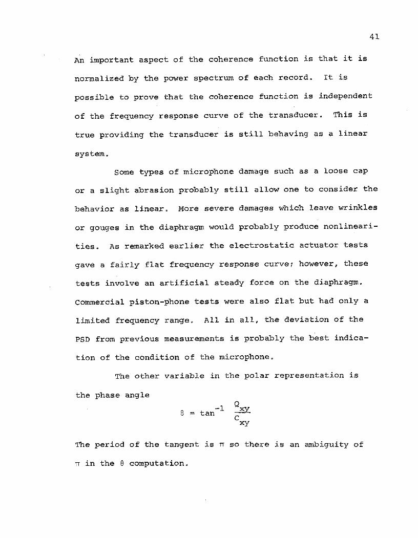
The other variable in the polar representation is

the phase angleQ

6 = tan xCxy

The period of the tangent is r so there is an ambiguity of

7 in the e computation.

42

The phase angle is more sensitive to the microphone

condition than the coherence coefficient. If the frequency

response curve shows a non-flat region, then there is theoret-

ically a phase difference in the response. This is true even

if the system is still linear.

It is customary to express the information contained

in the phase angle as a convective velocity. The equation

Uc 2rr FL

U e V L

defines the convective velocity, U , where /L is the distancec

separating the transducers. The Ames computer frequency

failed to produce curves of U /U . There were several reasonsC

for this. First, the tape was played at twice speed which

would give U /U twice its actual value. This tended to boost

the values out of the plot range. Second, the computer was

trying to pick the quadrant for 0 at the low frequencies

where the microphones show the most erratic response. Third,

the erratic response of the microphones themselves indicates

0 may be erroneous.

The coherence data is plotted on Fig. 45 for small

microphone separations and Fig. 46 for larger separations.

The two curves at the smallest separations show a high contri-

bution in low frequency decade. The microphones in each of

43

these correlations were in the same instrument plug whereas

all other correlations are between microphones in separate

mounts. The low frequency correlation may be an extraneous

signal resulting from this fact. Another possible explana-

tion would be a slow wandering of the sublayer which does not

correlate over long distances.

The remaining curves show a small erratic coherence

-3below F8*/V = 5*10 o This corresponds to the level portion

of the PSD plots. The left side of the peak holds about the

same shape as one progresses to larger separation distances.

These frequencies correspond to the falling portion of the

-2PSD curve since the peak in the PSD was about Fb*/V = 6-10 -2

As expected, the high frequencies lose coherence rapidly with

distance; at /8* = 33 (C = 5.5 inches) all eddies which

produced the right side of the PSD have decayed. After about

/8* = 22 the decay changes its character somewhat. The

coherence coefficient decays in value but seems to cover the

same bandwidth. The initial stages would correspond to

decay of the energy containing eddies and the second stage

would correspond to the so-called large permanent eddies.

All curves on the large separation plot, Fig. 46,

have been adjusted for boundary layer growth. A simple

average of the 6* at the two locations was used. At /65*40

44

and again at 50 there are two curves, one solid and one dashed.

The dashed curve is from transducers in the front portion of

the measurement region where the boundary layer is thinner.

A large eddy born in a thin layer may persist into the thicker

region of the boundary layer but it is no longer as large when

scaled by the local boundary layer thickness. Thus there is

a tendency for the low frequency end of the dashed correlations

to be low. From another point of view these curves give an

idea of the influence of the boundary layer growth on our

results.

Persistence of the large eddies is illustrated in

another way in Fig. 47. Maximum coherence is plotted vs.

distance. The maximum coherence coefficient is always in the

low frequency portion of the PSD so this is essentially a

plot of the large eddy decay.

Convective velocities would complete the picture;

unfortunately these data are probably no good. Figure 48

displays three graphs with narrow-band convective velocities

at various separation distances. These data were computed

by picking the phase angle from the Ames data and using the

formula previously given. One expects a low convective

velocity at small separations, say .5-.6, with possibly a

slight decrease with frequency. The curve at /65* = 3.3 is

45

reasonable. Increasing the separation should give higher

velocities but the curve at /6* = 6.8 drops. All the curves

from 21.9 on show a reasonable consistency. The trend toward

low values at low frequency is not explained although Wills

has suggested such a tendency (based on one data point).

The reason we put such little faith in the data is

shown by the dashed lines. At /6* = 11.7, 51.5, and 54.2

two calculations were made and both are shown. These calcula-

tions had the phase angle changed by 1800. Recall that this

is the ambiguity in the arctangent function in the calcula-

tion. This illustrates how the calculation changes with a

change in the phase angle. Since the PSD's showed some damage

to the microphones, which probably changed the phase angle,

we do not think this data is valid.

46

V. SUMMARY

The static pressure survey located a region of con-

stant pressure on the cylindrical portion of the forward

fuselage. The region was about 40 inches long and 10 to 15

inches wide. Pictures of tufts taken from another airplane

showed that the flow was aligned with the fuselage at the low

airspeeds. Tests were conducted at 55, 60, and 65 mph for

this reason.

The boundary layer velocity profile was measured at

three locations using a traversing pitot tube. When transi-

tion to turbulence was natural, the aft measuring station had

Reynolds numbers, Re *, of 4000 to 7000. This is moderately

low compared to other test situations. The forward measuring

station had a value around 2000-3000, which means the turbulent

layer is very young. Shear stress at the aft position was

typical of a classical zero pressure gradient layer but the

wake strength, R, showed a tendency to be low (.5) compared

to a value of .6 now quoted for a high Reynolds number layer.

The forward measuring location had a value around .2 which is

the proper trend for a layer not far from transition.

When the boundary layer was tripped, both forward

and aft locations had Reynolds numbers in the moderate range,

4000-9000, with fully developed turbulence. The wake strength

47

was now somewhat high and the shear stress correspondingly

low compared to nominal values. The deviations were well

within the range of experience encountered in typical test

situations.

Microphone measurements gave rms values which tended

toward .005 x q and 1.9 x T when extrapolated to zero micro-w

phone diameter. These values are at the low end of previous

results. The results showed slightly less scatter when

normalized by T . Since the tests were at moderate Reynoldsw

number, there was a larger change in T and a better opportunityw

to observe this trend. The power spectra of the fluctuations

also gave slightly better correlation with different airspeeds

and microphone diameters when normalized with T rather than q.w

The shape of the spectra was flat at very low fre-

-3quencies (F6*/V ! 6 * 10 3; F 50 Hz). There was a large

scatter in this region and the source of these components

is uncertain. The spectra then rose to a peak about F1*/V =

-26 - 10 . The rise was almost proportional to F whereas

some published theoretical conjecture would give F2 It may

be that an F region exists at the extreme low frequencies.

The peak value is in agreement with other comparable experi-

ments. Application of Corcos correction to three different

microphone sizes gave reasonable correlation and a fall off

rate corresponding to Willmarth's data.

48

The small 1/4 inch diameter microphones were suscep-

tible to damage and gave erratic spectra as the program

continued. Spatial correlation tests were conducted primarily

with these microphones. Of the four flights for which data

was reduced, only the first was good enough to analyze and

report. The convective velocities on this flight are thought

to be erroneous because of phase errors introduced by the

microphones. On the other hand, the coherence coefficient

is unchanged by a frequency response change and this data

is fairly good.

The coherence coefficient curves show two types of

change as the separation distance increases. At first, the

high frequencies decay and the peak lowers while the low

frequency side of the curve remains nearly the same. This

is characteristic of the energy containing eddies. After

frequencies higher than the peak PSD frequency have decayed,

the second type of decay beings. In this decay the band-

width of the coherence is about the same while the level

continues to decrease. This may characterize the large

"permanent" eddies. The nondimensional frequencies for the

correlation tests are lower than usual experiments have

achieved and it is unfortunate that a complete set of data

with convective velocities was not obtained.

49

REFERENCES

1. Hodgson, T. H., "Pressure Fluctuations in Shear FlowTurbulence," Ph.D. Thesis, University of London, 1962.

2. Proceedings, AFOSR-IFP-Stanford Conference on Computationof Turbulent Boundary Layers. Volume Two, D. E. Colesand E. A. Hirst ed. Stanford University publisher.

3. Wieghardt, K. and Tillmann, W., "On the Turbulent FrictionLayer for Rising Pressure," NACA TM 1314 (1951). Alsosee Ref. 2.

4. Wills, J. A. B., "Measurements of the Wave-Number/PhaseVelocity Spectrum of Wall Pressure Beneath a TurbulentBoundary Layer," JFM, 45, 1, pp. 65-90 (1970).

5. Lim, R. S. and Cameron, W. D., "Power and Cross-PowerSpectrum Analysis by Hybrid Computers," NASA TMX-1324(1966).

6. Willmarth, W. W. and Wooldridge, C. E., "Measurements ofthe Fluctuating Pressure at the Wall Beneath a ThickTurbulent Boundary Layer," JFM 14, 2, pp. 187-210,1962.

50

LIST OF FIGURES

1. Schweizer 2-32 sailplane

2. Instrument Location

3. Tuft Study of Fuselage Flow

4. Pressure Survey Tap Locations

5. Typical Manometer Record

6. Pressure Coefficient, Pows A & B

7. Pressure Coefficient, Rows C & D

8. Pressure Coefficient, Rows E & F

9. Pressure Coefficient, Columns 1, 2, 3

10. Pressure Coefficient, Columns 4, 5

11. Pressure Coefficient, Columns 6, 7

12. Pressure Coefficient on Measuring Streamline

13. Microphone Array No. 1

14. Microphone Array No. 2

15. Typical Boundary Layer Pitot Traverse

16. Boundary Layer Parameters, 55 mph



19. Displacement Thickness vs. Unit Peynolds Number

20. Friction Coefficient vs. Reynolds Number

21. Wake Parameter vs. Reynolds Number

22. Shape Factor vs. Reynolds Number

51

23. Microphone Test RMS Histories



26. Tape Recorder Flutter Spectrum

27. Tape Recorder Flutter Test Signal

28. RMS Results

29. CpL vs. Indicated Airspeed

3. pL vs Microphone ize Parameter

30. C C vs. Microphone size ParameterpL

31. CpC f vs. Microphone size ParameterpL f

32. Power Spectra Correction Factors

33. Airspeed Effects on PSD, 1/4" microphone (Files 4523,24, 25)

34. Airspeed Effects on PSD, 1/2" microphone (Files 3924,25, 26)

35. Airspeed Effects on PSD, 1" microphone (Files 3933, 34,35)

36. Airspeed Effects on PSD, 1/2" microphone, tripped BL(Files 3927, 28, 29)

37. Effects of Tripping on PSD, 1/4" microphone (Files 4524,4527)

38. Effects of Tripping on PSD, 1/4" microphone (Files 3925,3928)

39. Effect of Microphone Location on PSD (Files 4538, 4543,3928)

40. Effect of Microphone Diameter on PSD (Files 4524, 3925,3934)

41. Corcos Correction applied to Fig. 40.

52

42. Microphone PSD Histories during Flights 92, 93, 94, 95

43. Microphone PSD Histories

44. Microphone PSD Histories

45. Coherence Coefficient at Small Separation

46. Coherence Coefficient at Large Separation

47. Decay of Maximum Coherence Coefficient

48. Convective Velocities

8OAU Cft.- $^*MaD A? .

Co~7 *L- 6 a- wi

7h4Mwtom ARRAy RIPFORE.xa bs10 (m Ce 6ws)

PvsssuRc TAP ARReAY COMIF747UMATIOAl

............... .... ......... ...........

milli1 R

N 'j:

T- 7]W-

qp

low:

41t6

40.

Z

Iti-

11111ij

i

III I

I; li

t t

58

0.3-

Cp F

Cp PLorT FO Row A

0 : 60 mA. 0

0.1 - A : 70mph e

cpa i0 030 50

"7,

C iQor i w 9w&

F i . &

59

/0 , .~ 3'O10 JO60

-0./ -0: OMPO

-0.2/

C Pl.or PoR R9ow C

01F

cpa30 50

-0.2

cp PLO7- AOW ROW D

FIG. 7

60

0./I

O~O

c- - x

-0.1 - /

O O 0 A7N

a-- -A: 70 MPM)

Cp Por =OR Row E

0

0./ -

/X

CP 40s o os0 Ix/0 0 46o60

~0.I

-o.

/G9 8

, ,, k: 70,MPAI

,=IG

61

20 30

-0. /

0 0

0-0.21- - A-- .- 70 MPN-0.2-

A

-0.3

/0 20

o:7 A M

Cp PoT 0R C-4Um0N 2

o. OS"

--- A A- -- A :7 ommq

C, PRono COI.JNu 2

0.05S

0--- 670Mph'

- OA-/--0

-0.1Cp PLoT FoR OwAA/- 3

FIG. 9

0/ ~z

5r NV/fl70)d

HdAY OL ~--

01 07 S

Nivn70

&0d- 107 V- -V

#orw '5-

Hd1*0

63

0.3

Q-.-Q: 60 M~pg

A- -. ~ 70 mr-J

0.2

0.

00

0.0

0 */AC0 /0 /A/30

-03, Q. ..... 60 MPH

-0.2 Cp PL-OT r-oR CoI.uA4,v 7

FIG. I

Flo. /20.9

0.7-roe rff/IS Ac'RV OAY X A MEASOIZED

06 AQM 7716 ofL4Sc/RemAJ St.4LEAMI4U,

ReftM 70c NO*SE O- IWE AICCAFr

0.S

CP 0.3-

0.2 ~~PEERhaWC lhva' (SrWMV~I83.50 '9

0

00 300 40m

70 Af O

-0.3 O

Cpo PLOT FVoR A,cq4c-r

,f296ypFo~ x-O /,v - Er-

Aae496 aV' 6 Z /A

7,.fQ

12 IS P v

.- 2.70"

3.9O-~ 22AS5

Y2 B k.U Tv-fe 1134 Cwo,-,-,2 i R.cAAWAA

PL1AAR, DEVELOPM4ENT or 7'Q4Mvso(ER ARRAY 'L/

F1 C. /3

s-rA- 83 5o" (m~om c7,-R vo--.) oR42.86" (FRaW j-O 1A, CpPL,)

/22

3.90

//4

9. 750.7r,-- 4136 Covij.e,vsoeAC',c4

X< 7-f 4/3 4 Cc,,YDNso 0,R~~ioA

PANAR LDevrLopmeA' op TeAmsDUCER ARRAY *2 O

BOUNDARY LAYER PITOT TRAVERSE

2

In InchesVz60mph

Alt. 7200 Ft.

Trem s5 OF . *

01

0n Dncesna6mic Prsur

Tern.-55F+

:4

:.9.

• , . " -'/

0 0 + , .. . __Dynomi¢ re's-V.

BOUNDARY LAYER PARAMETERS

55 M.P.H. INDICATED AIRSPEEDUcn 6 6* *

FLT. # (ft/sec) (in.) F Cf(Xl03) (in.) H(- ) RMS DEV. Re,

56 94.7 .750 .530 3.28 .115 1.391 .250 421057T 98.8 1.114 .715 2.86 .178 1.393 .228 660058 99.8 .731 .437 3.39 .107 1.380 .217 396059 100.5 .716 .510 3.32 .110 1.386 .141 410060 91.0 .743 .534 3.27 .114 1.395 .137 420062 93.2 .751 .515 3.29 .115 1.387 .167 423063T 90.1 1.097 .625 2.94 .168 1.379 .124 650074* 93.6 .658 .621 3.21 .107 1.407 .238 416075T* 84.9 1.050 .702 2.89 .167 1.394 .187 634076 93.4 .830 .757 2.92 .143 1.399 .223 578077T 91.6 1.235 .919 2.60 .208 1.417 .273 835080 91.4 .721 .701 3.04 .120 1.407 .178 493081 92.1 .712 .566 3.20 .111 1.391 .150 455086 90.4 .738 .590 3.19 .117 1.395 .106 446088** 92.1 .374 .190 4.22 .052 1.393 .247 198089T** 95.4 .748 .676 3.09 .121 1.414 .178 4660

T - Tripped boundary layer

* - forward plug in aft. mounting bracket

* - aft. plug of forward mounting bracket

Fig. 16


60 M.P.H. INDICATED AIRSPEED

U6 6 6* *FLT # (ft/sec) (in.) T Cf(X103) (in.) H( ) RMS. DEV. Re

56 100.8 .781 .496 3.25 .117 1.377 .176 4610

57T 104.4 1.191 .728 2.78 .189 1.387 .286 7610

58 103.4 .766 .426 3.35 .111 1.370 .288 4330

59 106.3 .760 .460 3.29 .111 1.373 .133 4520

60 98.8 .790 .490 3.23 .118 1.371 .128 4810

62 99.6 .763 .468 3.28 .113 1.369 .181 4600

63T 95.7 1.104 .716 2.81 .175 1.387 .137 7300

74* 95.3 .699 .562 3.18 .109 1.384 .154 474.0

75T* 92.3 1.083 .789 2.75 .176 1.400 .274 7380

76 101.6 .860 .727 2.88 .140 1.397 .129 6290

77T 98.8 1.316 1.033 2.44 .228 1.424 .241 10,060

80 97.1 .737 .710 2.98 .122 1.402 .168 5400

81 100.5 .754 .643 3.03 .122 1.384 .350 5550

86 95.5 .763 .589 3.14 .119 1.391 .097 4840

88** 96.9 .416 .192 4.05 .057 1.373 .218 2380

89T** 102.6 .819 .843 2.83 .140 1.425 .131 5830



** - aft. plug of forward mounting bracket

Fig. 17


65 M.P.H. INDICATED AIRSPEED

U 6 6* 6*

FLT. # (ft/sec) (in.) 7 Cf(X103) (in.) H( ) RMS. DEV. Re

56 124.1 .852 .560 2.99 .128 1.362 .105 652057T 113.2 1.247 .858 2.60 .205 1.398 .123 915058 118.8 .818 .581 3.04 .125 1.376 .161 583059 126.8 .791 .542 3.06 .119 1.366 .129 591060 108.6 .815 .528 3.12 .123 1.367 .121 552062 102.5 .811 .478 3.15 .118 1.360 .092 556063T 105.0 1.153 .762 2.70 .184 1.384 .082 855074* 105.9 .729 .601 3.05 .113 1.383 .187 5550

75T* 100.7 1.193 .881 2.58 .196 1.403 .938 911076 109.0 .940 .743 2.78 .150 1.389 .165 745077T 107.3 1.372 1.089 2.34 .238 1.426 .199 11,674

80 106.8 .787 .701 2.90 .126 1.391 .221 629081 109.2 .820 .678 2.90 .130 1.385 .284 655086 104.9 .852 .601 3.00 .135 1.367 .217 618088** 105.0 .439 .249 3.85 .061 1.368 .260 280089T** 110n7 .819 .931 2.71 .144 1.430 .093 6550



* - aft. plug of forward mounting bracket

CFig. 18

Fig. 18

FIG. 19

7777 A

77U A

A

* 76GO76 A 76

cn AA A A

0 A

0~j 1 0 55 MPH

w 0J 55 MPH, TRIPPEDwu 0 60MPH

-JQ 60 MPH, TRIPPEDCL

(n A 65 MPH

A 65 MPH, TRIPPED

44~oo 5~ 5b0OUNIT RE WOLOS NUPV1ER Re,

fp 0 55 MPH

4.0 Op ] 55 MPH, TRIPPEDx4 0 60 MPH

Afp 0 60 MPH, TRIPPED

A 65 MPH

6 A 65 MPH, TRIPPED3.6 WIEGHARDT EXP.

0

O0

U-

ZO

3.2 3

U-

20O©

2. p -A

S2000 4 6000 8

REYNOLDS NUMBER Re8

F2G. 20

pfp

13 0 El © Q

LJ

0 5 MHTRIPPED

00

S60 MPH, TRIPPED

2000 4 6000 8

REYNOLDS NUMBER Re&*

FIG. 21

O 55 MPH

0 55 MPH, TRIPPED

1.6 A 60 MPH

A 60 MPH,TRIPPED

S65 MPH

S65 MPH,TRIPPED

1.5 -WIEGHARDT, EXP

I

1.4 Ou fP fp

CL

1.3-

2000 4 6000 8REYNOLDS NUMBER Re*

FIG. 22

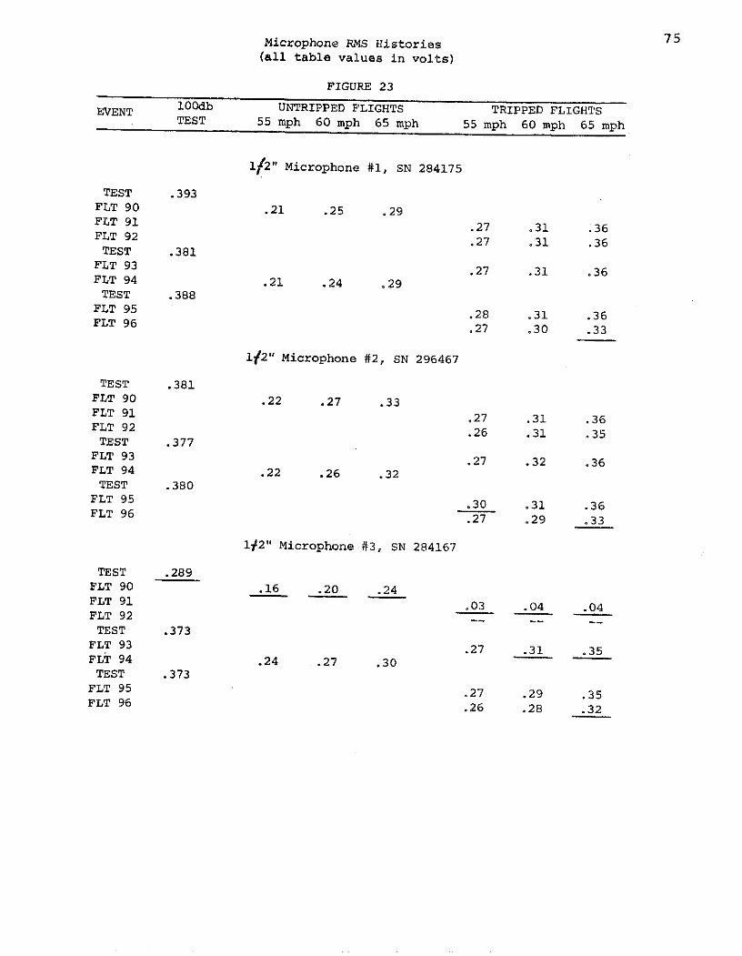
Microphone RMS Histories 75(all table values in volts)

FIGURE 23

EVENT 100db UNTRIPPED FLIGHTS TRIPPED FLIGHTSTEST 55 mph 60 mph 65 mph 55 mph 60 mph 65 mph

1/2" Microphone #1, SN 284175

TEST .393FLT 90 .21 .25 .29FLT 91 .27 .31 .36FLT 92 .27 .31 .36TEST .381

FLT 93 .27 .31 .36FLT 94 .21 .24 .29TEST .388FLT 95 .28 .31 .36FLT 96 .27 .30 .33



FLT 93 .27 .32 .36FLT 94 .22 .26 .32TEST .380

FLT 95 .30 .31 .36FLT 96 .27 .29 .33

l/2" Microphone #3, SN 284167

TEST .289FLT 90 .16 .20 .24FLT 91 .03 .04 .04FLT 92 -

TEST .373FLT 93 .27 .31 .35FLT 94 .24 .27 .30TEST .373

FLT 95 .27 .29 .35FLT 96 .26 .28 .32

76

EVENT 100db UNTRIPPED FLIGHTS TRIPPED FLIGHTS

TEST 55 mph 60 mph 65 mph 55 mph 60 mph 65 mph

112" Microphone #4, SN 296614


FLT 93 .28 .32 .37FLT 94 .24 .27 .32TEST .388FLT 95 .28 .32 .36FLT 96 .27 .29 .34



FLT 93 .43 .50 .58FLT 94 .41 .46 .51TEST .457FLT 95 .42 .47 .53FLT 96 .43 .47 .53TEST 1.129


TEST .745FLT 90 .62 .70 .80FLT 91 .66 .78 .86FLT 92 .65 .73 .83TEST .781FLT 93 .68 .78 .89FLT 94 .63 .72 .83TEST .693FLT 95 .56 .65 .72FLT 96 .59 .62 .75TEST

FIGURE 2577

EVENT 100db UNTRIPPED FLIGHTS TRIPPED FLIGHTSEVENTTEST 55 mph 60 mph 65 mph 55 mph 60 mph 65 mph


TEST .456FLT 90 .38 .42 .50FLT 91 .41 .45 .53FLT 92 .39 .45 .53TEST .434FLT 93 .39 .45 .49FLT 94 .36 .40 .48TEST .465

FLT 95 .40 .45 .52FLT 96 .39 .42 .51TEST 1.317


TEST .378FLT 90 .31 .35 .41FLT 91 .34 .40 .42FLT 92 .33 .38 .44TEST .388FLT 93 .35 .41 .47FLT 94 .34 .37 .45TEST .388

FLT 95 .38 .45 .50FLT 96 Microphone not flush .31 .33 .38FLT 96 .31 .33 .38



FLT 93 .37 .42 .47FLT 94 .33 .38 .44TEST .413

FLT 95 .38 .42 .48FLT 96 .37 .39 .46



FLT 93 .45 .52 .62FLT 94 .41 .46 .55TEST .572

FLT 95 .52 .60 .68FLT 96 Microphone protruding .68 .76 .87

SPECTRUM

12

10i-1

1

10-1

0 10

-9

10-8

10

-7

10-6

lo-s

I I

I I

I.15

1i

i_1

11

a a

1lI 0-

8

toh

0""

rn

a

m

S

MIS

a

OC

33

Cq

Sc

FIG. 27

- I I . I I I I I J ' I I I ' t t , t ! ! .I I I I I

CLEVITE CORPORATION/BRUSH INSTRUMENTS DIVISION

CLEVELAND. OHIO. PRINTED N U SA

- -- 74--

-

/--, )- -) . , i w 1 I

ga. .o/r-, 4-,. '' P - P -.,5,,=

FIGURE 28a

RMS of Pressure Fluctuations C =p 2 /qPx

C C CFLIGHT INDICATED FILE T PI PL L d

(MIC SIZE) AIRSPEED NUMBER TEST PSD LOOP C -1 PSFINTEGRAL

5394 34x -3 -3 -356 55 3924 3.42x10-3 3.76x10 3 4.04x10-3 1.235 3.18 7.69

(1/2") 60 3925 3.44x10-3 3.69x10-3 3.98x10- 1.225 3.15 8.8965 3926 3.07x10 3.50x10 3.70x10- 3 1.236 2.87 11.18

57 55 3927 4.06x10 3 4.62x10- 3 4.82x10 - 3 1.69 2.06 8.2(1/2") 60 3928 3.89xiO 3 4.35x10- 3 4.61x10 - 3 1.658 1.95 9.4Tripped 65 3929 3.71x10 - 3 3 .98x10-3 4.33x10- 3 1.665 1.79 11.4

58 -3(1/4") 55 3930 6.22x10-3 6.60xl0 3 6.88xl0-3 2.024 1.56 8.2

Sensitivity 60 3931 6.48xI0-3 6.74x10-3 7.52xl0 3 2.244 1.51 9.0Unknown 65 3932 5.47x10 5.55xi0 5.18lx0 - 3l 2.03 1.35 12.4

59 55 3933 2.33x10- 3 2.39x10- 3 2.74xl0-3 .826 6.69 8.3

(11 022xO- 3 .86 6.69 8.3(1)60 3934 2.21x10 -3 2.28x10- 2.64xl10 .801 6.63 9.665 3935 2.21x10 2.30xl0o 2.64xl0 - 3 .863 6.23 11.2

62

(1/2") 60 4520 3.35x10 3 3.45x103 3.71x10 3 1.039 3.26 8.95

63(1/2") 60 4518 3.89xl0 - 3 3.80x10- 3 3.95x10- 3 1.406 2.10 9.1Tripped

0o

FIGURE 28b

C C C CFLIGHT INDICATED FILE PT PI PL PL d q

(MIC SIZE) AIRSPEED NUMBER TEST PSD LOOP Cf YT PSFINTEGRAL

80 -3 -3 -3(1") 60 4519 2.15x10 2.16x10 2.23x10 .734 6.07 9.5

-3 -3 -355 4523 4.73x10 4.75x0 5.00x0l 1.567 1.58 8.3281 -3 -3 -3(1/4") 60 4524 4.23x10 3 4.60x10 4.61x10 1.521 1.38 10.10

65 4525 3.90x10 4.26x10 4.21x10 1.450 1.29 12.22

92 50(1/4") #1 4529 4.83x10- 3 4.68x10-3 4.52x10-3 1.59 1.04 9.45(1/4") #2 4531 4.42x10 4.73x10 4.69x10 1.67 .97 9.45(1/4") #3 4528 4.45x10- 3 4.59x10-3 4.19x10- 3 1.50 .95 9.45

-3 -3 -3(1/4") #4 4527 4.41xi0-3 4.57xi0-3 4.50xI0-3 1.61 .92 9.45(1/4") #5 4535 4.12x10 4.24x10 4.nx10 3 1.48 .92 9.45(1/4") #6 4527 4.3 9x10-3 4.35xl0 - 3 4.57xl03 1.64 .92 9.45

(1/2") #1 4529 3.58x10 3 3.57x10 3 3.67xl0 3 1.24 2.79 9.45-3 -3 -3(1/2") #2 4534 3.66x10 3.66x10 3.67x10 1.32 2.02 9.45

(1/2") #4 4527 3.69x10 3.47xl0 3.55x10 1.31 1.86 9.45

93 60 -3 -3 -3(1/4") #1 4538 5.06xl0 5.20x10 4.22x10 1.49 1.04 9.05(1/4") #2 4537 4.94xI0 5.44xlO 5.16x10 3 1.84 .97 9.05(1/4") #3 4537 5.65xl 4.69x10 3 4.69x10 1.68 .95 9.05(1/4") #4 4536 4.98xl03 4.71xl03 4.87x0 1.75 .92 9.05(1/4") #5 4544 4.77x10 4.96xl0 3 4.77xl03 1.71 .92 9.05(1/4") #6 4536 4.97x10 5.42x10 5.69x10 1.83 .92 9.05

98,1 £TXE8*E E- TX8S*E f# (a,/i)

£01 -T88E E- TX8L*E T99f' E# (.Z/T)£0z -TXt70*t C- TXZO* T99t' Z# (..Z/T)

6L*ZE OTXOOt E- XE6*EVSt T# (.Z/T)

SU 6 -OTXLO'L C- Txt9'L 9sSt7 9# (~7T

BUB Z6 E TX66*V E- OXTZ'S Z91 # (..,/T)

BU Z6 E0TX6V' , E-TXtV£ , 09st7 t,# (..WT)

8E*8 96 -OTXLL*V E- TXIV8*V £Gt # (1WtT)

SE'a L6' -l~~ -TZ* gt #(.7T

SUB VO0T E- TX96*V E£TXV7L*V9t, 097 T# (..t'/T)

6S*8 98*TE OTXELC E-OTx9S*E E-OXOP SIPt# (,./T)8S801zE-OX88E E- 1X66*E E-OIXE8* c£st' E# (.,Z/T)

89,8 £01 E OXT6* E-OTXL.6* E- TXE6*V Z9t # (,./T)

89,8 6L'ZE £1XT6*E E- 1X86*E C- 1XS6*E SDt T# (,.Z/T)

BS' WC 0Tx6Z*S C- TXES~g E 0Tx9T~ LtA'v4 9# (11W1/)9S*8 Z6 E 1x6L*V C- TXL9'V E-OpcXcO.S stS#(t/T8S,8 W E-OIXV9*S E- 1X69*9 C- 1x9L*S Lt7SA7 V7# (11t'/T)

89,8 96'E-OTX8V CTxBBSfr E-tx. £OTX06*f7 9f'st E# (11WT)

99,8 L6* £-OXLE*i7 E-TV* E-TX 9tST7 Z# (ui',/T)8S*8 T70-T C- OX78', C- TXDS'D E ~OTXTO*G S T# (13f'/IM

£09 9

98*T 9E* E OTXOL'E C- XS9*E E OTXL8*E 8ESt, f,# (1*Z/i)8V~ BT E-OTXS8*E E- X06*E E01X68CE £!?s7 E# (../T)

zoz 6UT E01XL8'E E01X90*V E- TX96'E Ett # (,../T)

6LZ OUT E OTXL8' E OTXE6CE E OTXSLCE 0tlgt7 T# (../T)

3 dOO'I GSd iJi USS1I, 0laalIv (azls DIN)

p 1C lI d aia Galvoiatmi IH£2i'ia

FIG. 29

S5x10 1.6

O

4 1.4

3 1.0W

2 8

0

I-_

3 1.U)

rx 0a_ an.--J

0 FLT 56 1/2" MIC C-2 lxi0 3 A FLT 57 1/2" MIC TRIPPED o .4

[0 FLT 59 1. " MIC

FLT 81 1/4" MIC

55 ,60 65 5 60 65

INDICATED AIRSPEED INDICATED AIRSPEED

FIGURE 30

x5xo10-3_ x

cm A

- -3 F

0 FLT 56 1/" MICA FLT 57 1/2" MIC TRIPPED

U- E3 FLT 59 1 " MICLUJ

2x10 -3- FLT 62 1/2" MIC PLuA FLT 63 1/2" MIC TRIPPED

0 FLT 80 1 "1MIC

x FLT 93 TRIPPED

0 2 3 4 5 6

MICROPHONE SIZE d/*

FIGURE 31

2.0

x1.8 x

x

1.6

o 1.2

I--

8 1.4xg

Co 1.2 so

1.0 0 FLT 56 1/2" MIC

." A FLT 57 1/2" MIC TRIPPED

.8 FLT 59 1 " MIC E

, FLT 62 1/2" MIC.6 , FLT 63 1/2" MIC TRIPPED

o FLT 80 1 " MIC

.4- FLT 81 1/4" MIC

* FLT 92 TRIPPED

.2- x FLT 93 TRIPPED

1 2 3 4 5 6 7

MICROPHONE SIZE d/3

Fig. 32

Power Spectra Correction Factors 86

Coordinate GV F* GV2 V 2 V

Q S* 5Correction C CMultiplier 1 2 3 4

File #

3924 8.72 .115 1.25 x 105 .750

3925 12.46 .118 1.78 x 105 .7885

3926 7.42 .126 1.25 x 10 .839

3927 5.16 .172 1.01 x 105 1.076

3928 5.22 .185 1.08 x 105 1.166

3929 4.52 .199 1.10 x 105 1.211

3930 7.83 .103 1.00 x 105 .704

3931 9.47 .111 1.23 x 105 .766

3932 6.59 .115 1.09 x 105 .753

3933 8.14 .105 1.13 x 105 .684

3934 8.56 .108 1.15 x 105 .677

3935 8.06 .116 1.29 x 105 .771

4520 1.764 .567 .243 x 105 3.829

4521 2.292 .436 .461 x 105 2.75

4522 1.646 .608 .307 x 105 3.67

4523 1.784 .560 .271 x 105 3.59

4524 1.640 .610 .289 x 105 3.77

4525 1.544 .648 .289 x 105 4.12

4527 (MIC 4) 2.198 .455 .450 x 105 2.88

4527-4563:

Track 11 3.03 .330

Track 1 2.469 .405

Track 2 2.230 .435

Track 3 2.260 .442

Track 4, 5,6, 10, 11, 2.198 .45512, 13

Track 14 2.02 .495

Remarks: Files 3924 through 3935 corrected for errors in Q, V,and L. Files 4520 through 4527 corrected for errorsin L and tape playback speed.

Airspeed Effects On PSO, 4'Aic

_ 87

Indicated Airspeedi

6100 Mp... IPH

1 -6 ..... ... . ".-

iot it

lrr/v

w**

mp

- * *

lal

" t

10 10

F /

1.0. 3

FiG. .. 33

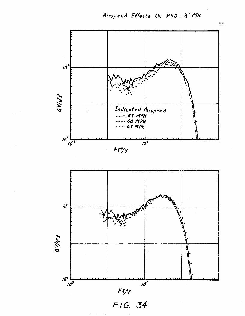
Airspeed Efects On PSOY, "'/ic

* *

Ii 88

Indicated Airspeed

.... 60 1Pk0 a*006 T/fPH

160 /0

* '.I.- V

/ /0oo

G 34-I ~F 11VF1T 34

F~e. t

Airspeed Effects On PSO, I"'AI'c

89

-A* 1

6.

, ** *

id' /*

]~~~n di c . e d. A a 'It'tP P'rs pee d

...... . . . .. , . , . .

Ftf/v

FIG. 35

* 9

" II-

gInicte As"e

] A I i- I mr I 1III I

w I•

-- - 6 ? o"* *' * 5 f /

Fie. 35

Airspeed Effects On PSD, fA~" c, Tr,Pfded B.L.90

/0

; ..

Zndica fed Arrspeed- 6' P

--- 60 HPH

A fP

* * • 65 /IpH/

/A-2

/4 Ida

FI"7

,.. .

.*.

/0'

/F /0. 36Ft/v

F/G. 36

EffectS Of Tripoij 00 PSD, 4'V"~. 91

--Unfrippe

- ripped

1F 4 AP

FIG. 37

5ff~f sOf ;rhpf/oy 04PDi~/,92

ta- Tripped

- -- Un~tripped

/.-

FIG 38

93

£LffectS Of If/erophone locaion On PS)

101

-%4 V

- Fwd.--- Aft. "'x xx u4pper *....... Lower :.

Fr/v

F/G. J9

Effe cfs Of /Mrcrophone Diometer 0w PSD

94

go%

* .*

0i

% ' - br

o--fo/'f/C

•

-33

10o /

FI//Fo a. 4to a

T44

II1

I

I-3 I

Fs/v

FI G. 40O

95

Corcos Correctiuan Applied To Fj . 40

Im**

F f*/v

Fic 4/

Af roph '/e #z//i'r

g , .. 96

Ion'

S- Fie. 92

040 4 t

.1

Ids FLi

F..... 42

* .' . - * *, 1 " .,.• *. ... : .. . ..- . ..,,

.. " * .. ...*'*

...- , ,.. . . .*

'" FI..-. 42.,..:" ".

F16. 43 - Ai ekn4PSI'Hseoa

FL/U

AI/A

FL/y tr

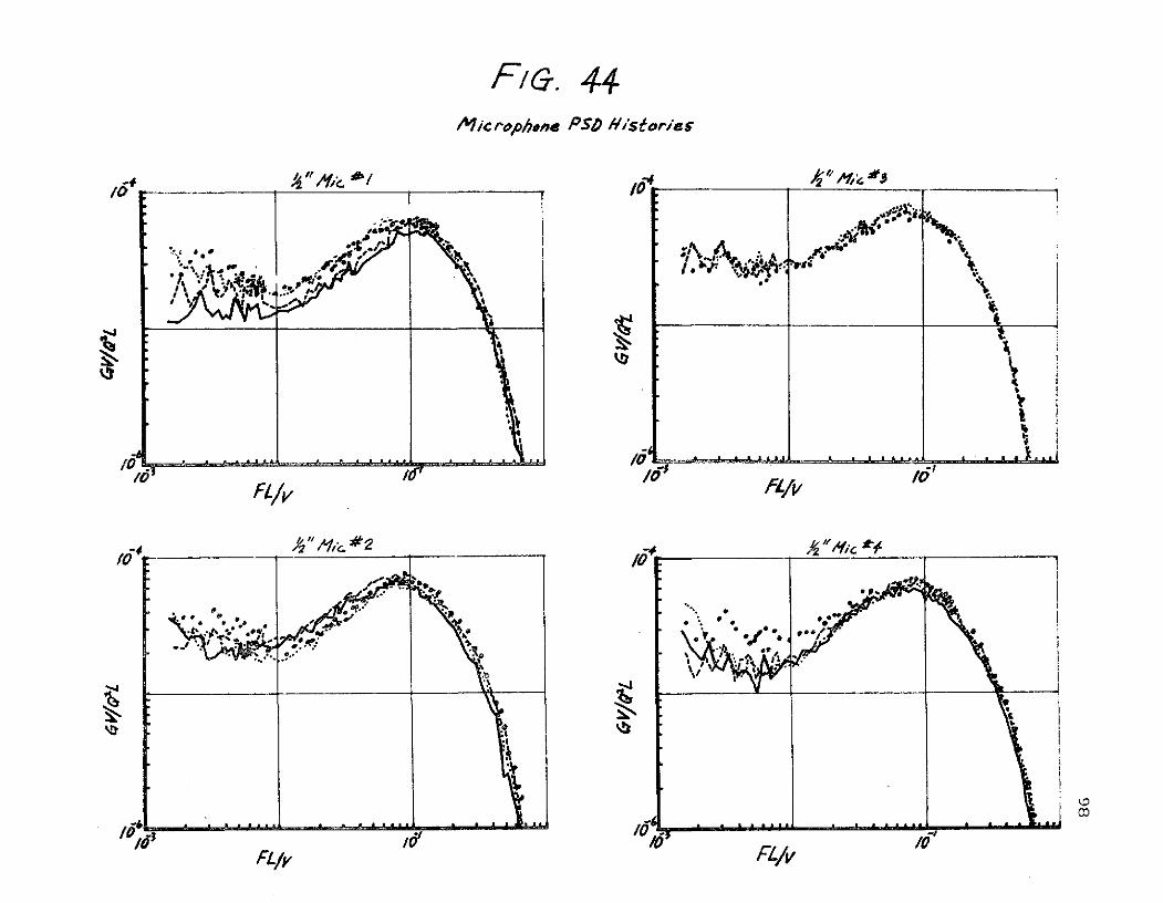
F/G. 44

Alic rophone PSI Histories

.~~F C - 4- f 44M

poif

F/0 11

I A AI IR A ,o/Vo. tol• °° - , .* " ." Oo 4-

n '. ...."..o. , . a a m s e . a -

,II

/0 ,L/V /0 /0' F, //v

99

-K ±o

20

0 00

1.

l.~IG 45," J

*2.5 C

| a I III .U L . _ _i i i .,

-C-

0 1__ _"

Fi G. 4,5

100

.30

TI_______ so

U7 2

V

.100

/0+ 10 10 1

-7

F, 4 6

so

FG 47

FIG 47

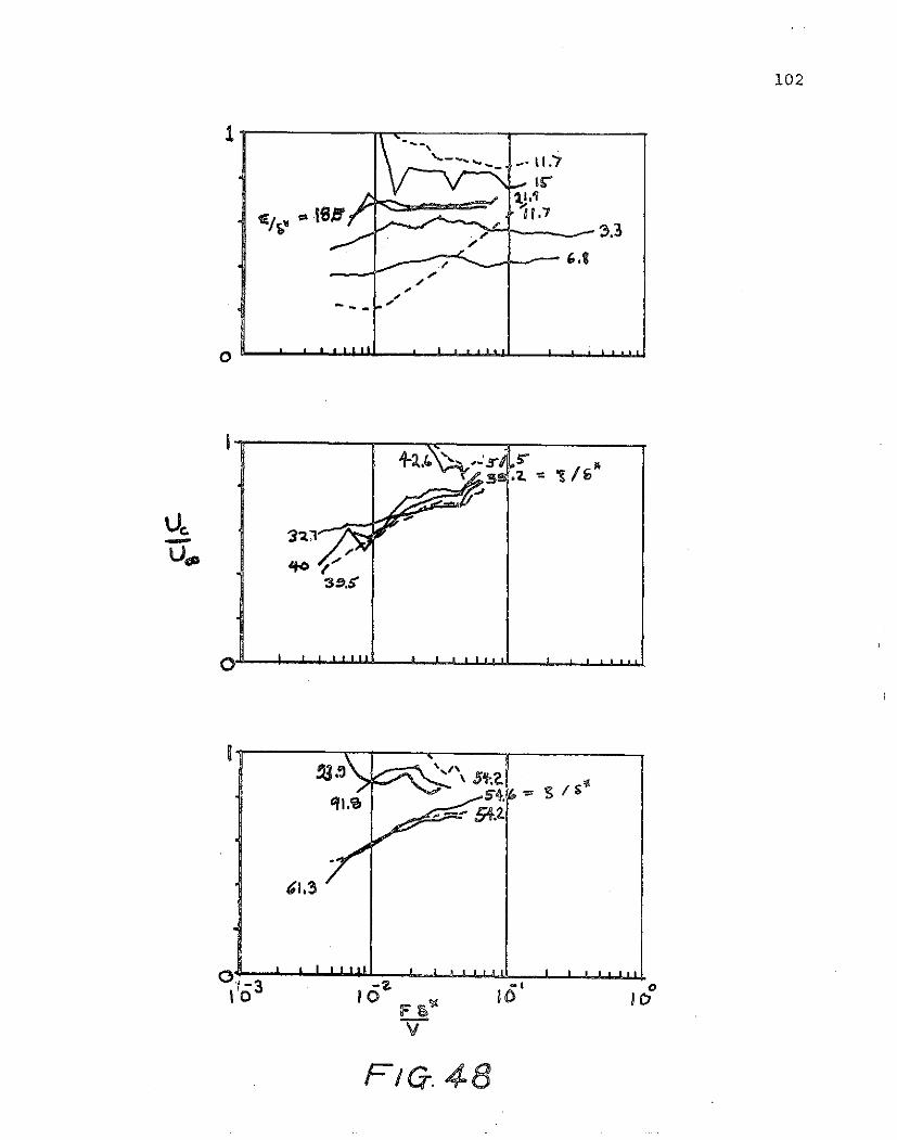
102

0

ur-.

0 j I ilia.p u I I *m .

I

'1-3

10 67-v6

Fla.4

Documents

III. PRESSURE FLUCTUATION MEASUREMENT · NASA Grant NGR 37-002-083 ... Tripping was necessary in these tests in order to have a ... ratio of 34:1 is obtained