St 412/512 page 45

III. Inferential ToolsA. Introduction to Bat Echolocation Data (10.1.1)

1. Q: Do echolocating bats expend more enery than non-echolocating bats and birds, after accounting for mass?

2. Strategy: (i) Explore (resolve need for trans-formation) (ii) Is 3 par-allel lines model ok? (iii) If so, answer question by comparing ne-bats line to the two others.

2 3 4 5 6 7

Log of mass

0

1

2

3

4

Log

of e

nerg

y ex

pend

iture

non echolocating batsbirdsecholocating bats

St 412/512 page 46

3. A note about different parameterizations for a factor

a. Example: the factor TYPE has 3 levels (e-bats, birds, ne-bats)

b. Consider the model µ(µ(y|x,TYPE)= x + TYPE. We have some choices about which of the 3 indicator variables to include

c. If we include two indicator variables, the level whose indica-tor isn’t included is the “reference level”; i.e. if µ(µ(y|x,TYPE) = ββ0 + ββ1x + (ββ22Itype2 + ββ33Itype3) where Itype2 and Itype3 are indi-cator variables for levels 2 and 3 of “type”, then ββ0 is the intercept for level 1; ββ22 is the amount by which the mean of y is greater for level 2 than for level 1 (after accounting for x) and ββ33 is the amount by which the mean of y is greater for level 3 than for level 1 (Display 10.5)

d. Another parameterization is (ββ1Itype2+ ββ22Itype2 + ββ33Itype3) + ββ44x (without a ββ0). In this, ββ1, ββ2, ββ3 are the 3 intercepts

St 412/512 page 47

To include a factor so that the firstlevel is the reference level (“treat-ment contrast” in S-PLUS), includethis term in the formula

If necessary, changedata type to “factor”

St 412/512 page 48

To include a factor so that eachlevel gets its own intercept, drop

model formula term “ - 1”the overall intercept by using the

Note: R2 and the F-statistic do notmake sense when the intercept isdropped.

St 412/512 page 49

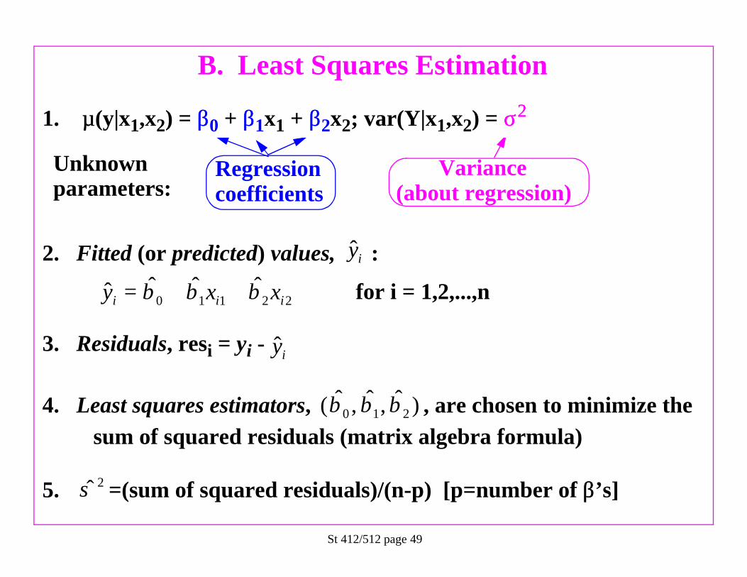
B. Least Squares Estimation

1. µµ(y|x1,x2) = ββ0 + ββ1x1 + ββ2x2; var(Y|x1,x2) = σσ22

2. Fitted (or predicted) values, :

for i = 1,2,...,n

3. Residuals, resi = yi -

4. Least squares estimators, , are chosen to minimize the sum of squared residuals (matrix algebra formula)

5. =(sum of squared residuals)/(n-p) [p=number of ββ’s]

Unknownparameters:

Regressioncoefficients

Variance(about regression)

ˆiy

0 1 1 2 2ˆ ˆ ˆˆi i iy x xβ β β= + +

ˆiy

0 1 2ˆ ˆ ˆ( , , )β β β

2σ̂

St 412/512 page 50

C. t-tests and CI’s for individual ββ’s

1. Note: a matrix algebra formula for is also available

2. If distribution of Y given X’s is normal, then

has a t-distribution on n-p degrees of freedom

3. For testing the hypothesis H0: ββ2 = 7; compare

to a t-distribution on n-p degrees of freedom.

4. The p-value for the test of H0: ββj = 0 is standard output

ˆ( )jSE β

ˆ

ˆ( )j j

j

t ratioSE

β β

β

−− =

2

2

ˆ 7ˆ( )

t statSE

ββ−

− =

St 412/512 page 51

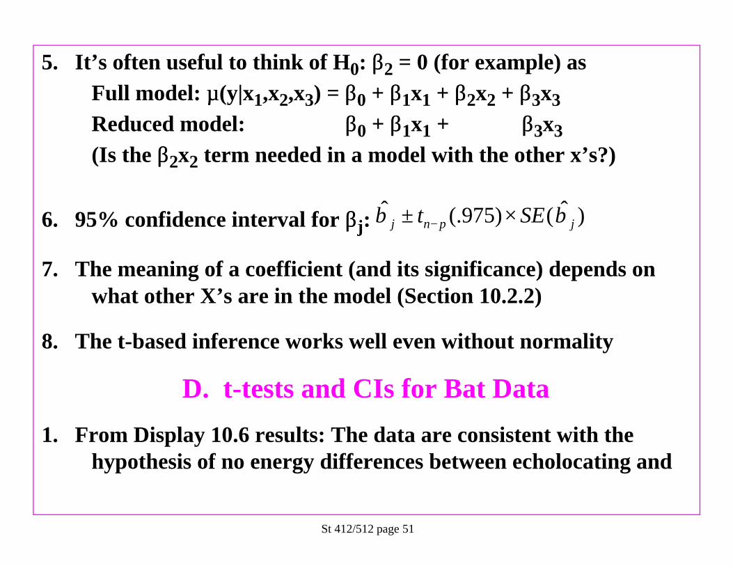
5. It’s often useful to think of H0: ββ2 = 0 (for example) asFull model: µµ(y|x1,x2,x3) = ββ0 + ββ1x1 + ββ2x2 + ββ3x3Reduced model: ββ0 + ββ1x1 + β β3x3(Is the ββ2x2 term needed in a model with the other x’s?)

6. 95% confidence interval for ββj:

7. The meaning of a coefficient (and its significance) depends on what other X’s are in the model (Section 10.2.2)

8. The t-based inference works well even without normality

D. t-tests and CIs for Bat Data

1. From Display 10.6 results: The data are consistent with the hypothesis of no energy differences between echolocating and

ˆ ˆ(.975) ( )j n p jt SEβ β−± ×

St 412/512 page 52

non-echolocating bats, after accounting for body size (2-sided p-value = .7)

2. But that doesn’t prove that there is no difference. A “large” p-value means either: (i) there is no difference (H0 is true) or (ii) there is a difference and this study is not powerful enough to detect it.

3. So: report a confidence interval in addition to the p-value.95% CI for ββ3: .0787 ± 2.12×.2027 = (−.35,.51).± 2.12×.2027 = (−.35,.51).

Interpretation (back-transform, e.0787 =1.08, e-.35=.70 and

e.51=1.67): It is estimated that the median energy expenditure for echolocating bats is 1.08 times the median for non-echolo-cating bats of the same body weight (95% confidence interval: .70 to 1.67 times).

St 412/512 page 53

E. Review of “variance”, “SD”, “SE”

1. var(y) = Mean{(y-µµ)2} (population variance)

2. SD(y) = {var(y)}1/2

3. var(y|x) = Mean{[y-µ(µ(y|x)]2} in subpopulation of y’s at x

4. var( ) = Mean{( - )2} (sampling variance)

5. SD( ) = {var( )}1/2

6. SE( ) = Estimate of SD( ), usually obtained by using

in place of the unknown (with associated d.f.)

β̂ β̂ β

β̂ β̂

β̂ β̂ σ̂σ

St 412/512 page 54

F. Reminder about interpolation and extrapolation

Y

XWe can safely make statements about the distribu-tion of y given x-values within the sampled range

Extrapola-tion involvesadditionalspeculation

?

?

1

2

St 412/512 page 55

G. Extra SS F-tests

1. Full model: ββ0 + ββ1x1 + ββ2x2 + ββ33x3Reduced model: ββ0 + ββ1x1

i.e. in full model, H0: ββ2 = β β33 = 0

2. Extra sum of squares = (Sum of squared residuals from reduced model) - (Sum of squared residuals from full model)

3. F-statistic = [Extra SS/Extra # of ββ’s]/

4. Display 10.10 example: Full: log.energy ~ lmass + TYPEReduced: log.energy ~ lmassOne can fit both models and get the SS Residual from the ANOVA table (as in Display 10.10), or...

2ˆ fullσ

St 412/512 page 56

5. Valuable short-cut in S-PLUS: Save model objects, then use “Compare Models”

(continued, next page)

St 412/512 page 57

1

Write namesof model objects,separated by “,”

2

Compare with Display 10.10

St 412/512 page 58

H. Special Cases of Extra SS F-test

1. F-test for overall significance of regression

Full model: ββ0 + ββ1x1 + ββ2x2 + ββ3x3 Reduced model: ββ0

Asks: are any of the x’s useful predictors of y?The calculations are laid out in the ANOVA table

2. F-test for a single coefficientIf full model has one more term than the reduced model, the F-test is equivalent to the (2-sided) t-test

3. For µ(µ(y|CAT) = CAT (i.e. a single categorical factor), the F-test

for overall significance is the one-way ANOVA F-test

St 412/512 page 59

I. Prediction and prediction intervals

1. Suppose

2. The estimated mean of y at x1 = 15 and x2 = 7 (say) is

3. The SE of the estimated mean at x1 = 15 and x2 = 7 is

= (matrix algebra formula; S-plus knows it and does the calculations in the “Predict” tab)

4. The predicted value of y at x1 = 15 and x2 = 7 is

i.e. predict y to be its mean value

1 2 0 1 1 2 2( | , )y x x x xµ β β β= + +

1 2 0 1 2ˆ ˆ ˆˆ ( | 15, 7) (15) (7)y x xµ β β β= = = + +

1 2ˆ[ ( | 15, 7)]SE y x xµ = =

1 2 1 2ˆPred( | 15, 7) ( | 15, 7)y x x y x xµ= = = = =

St 412/512 page 60

5.

6. 95% Prediction interval:

7. S-PLUS:

2 2 1/ 21 2 1 2ˆ ˆ[Pred( | 15, 7)] { [ ( | 15, 7)] }SE y x x SE y x xµ σ= = = = = +

sampling variance inestimating mean of yat those x’s

variance of an individual y about its (subpopula-tion) mean

1 2 1 2Pred( | 15, 7) (.975) [Pred( | 15, 7)]n py x x t SE y x x−= = ± = =

Create a new data set withcolumns named x1 and x2,with values x1

*, x2*

* *1 1 2 2ˆ ( | , )y x x x xµ = =

1 2ˆ[ ( | 15, 7)]SE y x xµ = =

SE[Pred] must be calc-ulated from these, and the formula in 5 above

2σ̂