Embed Size (px)
Citation preview
ii
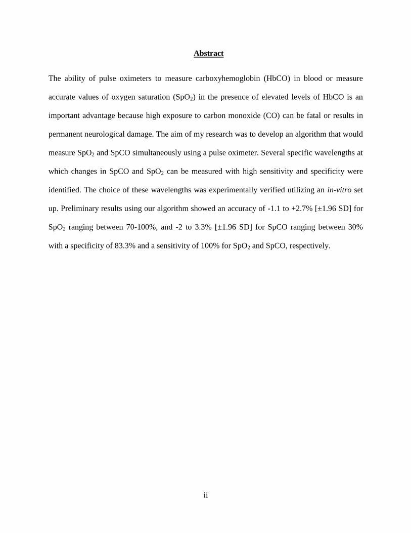
Abstract
The ability of pulse oximeters to measure carboxyhemoglobin (HbCO) in blood or measure
accurate values of oxygen saturation (SpO2) in the presence of elevated levels of HbCO is an
important advantage because high exposure to carbon monoxide (CO) can be fatal or results in
permanent neurological damage. The aim of my research was to develop an algorithm that would
measure SpO2 and SpCO simultaneously using a pulse oximeter. Several specific wavelengths at
which changes in SpCO and SpO2 can be measured with high sensitivity and specificity were
identified. The choice of these wavelengths was experimentally verified utilizing an in-vitro set
up. Preliminary results using our algorithm showed an accuracy of -1.1 to +2.7% [±1.96 SD] for
SpO2 ranging between 70-100%, and -2 to 3.3% [±1.96 SD] for SpCO ranging between 30%
with a specificity of 83.3% and a sensitivity of 100% for SpO2 and SpCO, respectively.

iii
Acknowledgements
I wish to convey my deepest appreciation to Prof. Mendelson for his expertise and assistance
throughout the course of my work.
I would like to thank Prof. Lambert and Prof. Chon for their valuable suggestions and many
helpful discussions.
I also wish to express my deepest gratitude to my family for their constant support and love.
This work was supported by the U.S. Army Medical Research and Material Command under
Contracts No. W81XWH-07-2-0106 and W81XWH-10-1-0529. The views, opinions and/or
findings are those of the author and should not be construed as an official Department of the
Army position, policy or decision unless so designated by other documentation.
iv
Table of contents
ABSTRACT ii
ACKNOWLEDGEMENTS iii
TABLE OF CONTENTS iv
LIST OF FIGURES vi
LIST OF TABLES xi
LIST OF ABBREVIATIONS xii CHAPTER 1. PHYSIOLOGICAL AND CLINICAL SIGNIFICANCE OF OXYGEN AND
CARBON MONOXIDE SATURATION 1
1.1. Oxygen saturation and its significance 1
1.2. Physiological and clinical effects of CO 2
CHAPTER 2. BACKGROUND ON PULSE OXIMETRY 6
2.1. SpO2 measurement using pulse oximetry 6
2.2. Current methods available for simultaneous measurement of oxygen
and carbon monoxide saturation using pulse oximetry 9
CHAPTER 3. SPECIFIC OBJECTIVES 11
CHAPTER 4. IN-VITRO MODEL FOR SIMULTANEOUS MEASUREMENT
OF SpO2 AND SpCO 12 4.1. Need for an in-vitro model 12
4.2. Description of in-vitro models 13
4.3. Experimental set-up 17
4.4. HbCO measurement using CO-Oximeters 18
CHAPTER 5. PRELIMINARY RESEARCH TO VALIDATE THE SENSOR
AND IN-VITRO MODEL 21
5.1. Methodology 21
5.1. 1. SpO2 experiments
5.1. 2. SpCO experiments 22
5.1. 3. Assessing the validity of the tissue simulator 22
5.2. Results 23
5.3. Discussion 25
5.3.1. SpO2 experiments 25
5.3.2. SpCO experiments 26
5.3.3. Assessing the validity of the in-vitro tissue simulator 27
CHAPTER 6. THEORETICAL MODELING FOR SIMULTANEOUS SPO2 AND SPCO
MEASUREMENT 28
6.1. Need for theoretical model 28
6.2. Beer-Lambert’s Law 29
v
6.3. Derivation of the theoretical model 31
6.4. Wavelength ratio selection 39
6.4.1. Validation of the theoretical model for r1= A (660/940) and r2= A (643/940) 41
6.5. Theoretical Simulations 42
6.5. 1. Simulations for wavelengths 660, 610, 940 43
6.5. 2. Simulations for wavelengths 660, 643, 940 45
6.5. 3. Simulations for wavelengths 660, 740, 940 50
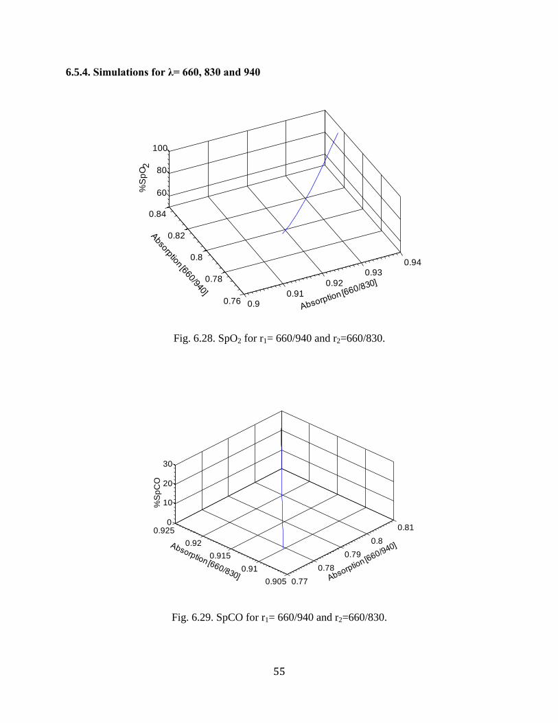
6.5. 4. Simulations for wavelengths 660, 830, 940 55
6.5. 5. Simulations for wavelengths 660, 880, 940 59
6.6. Discussion 65
6.7. Experimental verification of theoretical results 67
6.7. 1. Simulations for wavelengths 660, 610, 940 68
6.7. 2. Simulations for wavelengths 660, 643, 940 71
6.7. 3. Simulations for wavelengths 660, 740, 940 73
6.7. 4. Simulations for wavelengths 660, 830, 940 74
6.7. 5. Simulations for wavelengths 660, 880, 940 76
CHAPTER 7. ALGORITHM FOR SIMULTANEOUS MEASUREMENT OF
SpO2 AND SpCO 79
7.1. Thresholds used in the algorithm 80
CHAPTER 8. ALGORITHM TO CALCULATE SpO2 AND SpCO 81
8.1. Results 82
8.2. Discussions 85
CHAPTER 9. CONCLUSIONS AND FUTURE WORK 93
APPENDIX 96
REFERENCES 98
vi
List of figures
Figure Page
1.1 O2-CO-Hb dissociation curve. 3
2.1 Light absorption through the skin. 6
2.2 Absorption spectra of Hb and its derivatives. 7
2.3 Variation in DC absorption between R and IR wavelengths before (a)
and after normalization (b). 8
2.4 Wireless pulse oximeter device designed in our lab. 10
4.1 In-vivo calibration of a pulse oximeter sensor conducted on a volunteer. 13
4.2 In-vitro model developed by Reynolds et al. 14
4.3 In-vitro model developed by Edrich et al. 15
4.4 Mock circulatory system developed by Oura et al. (a).
Schematic representation of the double layered cuvette (b). 15
4.5 Experimental set up (a) a close up of the blood compartment
in the tissue simulator (b). 16
4.6 Absorption spectra for Hb and its derivatives. The vertical lines
indicate seven wavelengths used in our prototype sensor. 18
4.7 Absorption spectra of RHb, HbCO, HbO2, MetHb in the visible region.
The vertical lines indicate the wavelengths used in an IL 682
CO-oximeter. 19
5.1 Mean AC/DC plots obtained from three sets of SpO2 experiments. 23
5.2 Absorption spectra of HbO2 obtained from the literature. 23
5.3 Mean AC/DC plots obtained for three sets of SpCO experiments. 24
5.4 Absorption spectra of HbCO obtained from the literature. 24
6.1 Exponential decrease in light intensity as it passes through an
absorbing medium. 29
6.2 Theoretical simulation for SpO2 at r1= 660/940 and r2=643/940. 41
vii
6.3 Theoretical simulation for SpO2 (HbCO is absent) using two
wavelengths (r1= 660/940). 41
6.4 SpO2 for r1= 660/940 and r2=660/610. 42
6.5. SpCO for r1= 660/940 and r2=660/610. 42
6.6 SpO2 for r1= 660/940 and r2=660/610 . 43
6.7 SpCO for r1= 660/940 and r2=660/610. 43
6.8 SpO2 for r1= 660/643 and r2=660/940 . 44
6.9 SpCO for r1= 660/643 and r2=660/940. 44
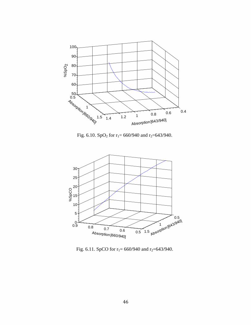
6.10 SpO2 for r1= 660/940 and r2=643/940 . 45
6.11 SpCO for r1= 660/940 and r2=643/940. 45
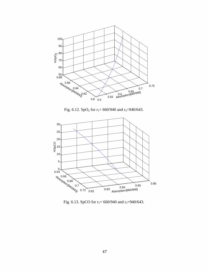
6.12 SpO2 for r1= 660/940 and r2=940/643 . 46
6.13 SpCO for r1= 660/940 and r2=940/643. 46
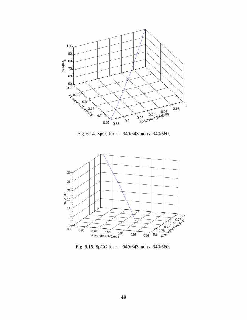
6.14 SpO2 for r1= 940/643and r2=940/660 . 47
6.15 SpCO for r1= 940/643and r2=940/660. 47
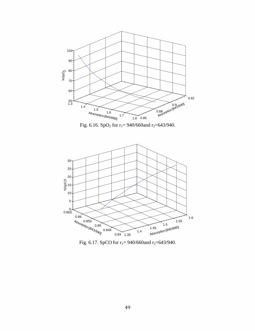
6.16 SpO2 for r1= 940/660and r2=643/940 . 48
6.17 SpCO for r1= 940/660and r2=643/940 . 48
6.18 SpO2 for r1= 660/740 and r2=660/940 . 49
6.19 SpCO for r1= 660/740 and r2=660/940. 49
6.20 SpO2 for r1= 660/940 and r2=740/940 . 50
6.21 SpCO for r1= 660/940 and r2=740/940. 50
6.22 SpO2 for r1= 660/940 and r2=940/740 . 51
6.23 SpCO for r1= 660/940 and r2=940/740. 51
6.24 SpO2 for r1= 940/660 and r2=740/940 . 52
viii
6.25 SpCO for r1= 940/660 and r2=740/940. 52
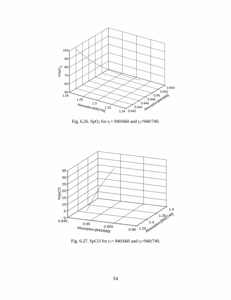
6.26 SpO2 for r1= 940/660 and r2=940/740 . 53
6.27 SpCO for r1= 940/660 and r2=940/740. 53
6.28 SpO2 for r1= 660/940 and r2=660/830 . 54
6.29 SpCO for r1= 660/940 and r2=660/830. 54
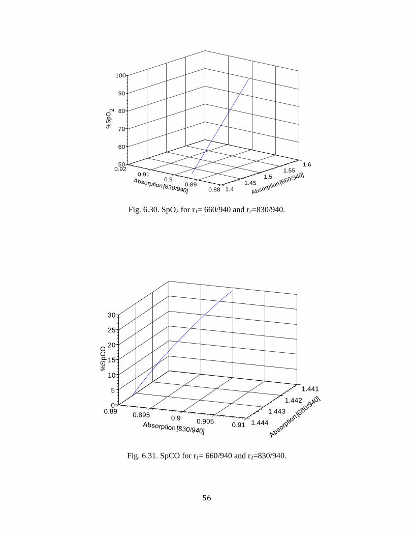
6.30 SpO2 for r1= 660/940 and r2=830/940 . 55
6.31 SpCO for r1= 660/940 and r2=830/940. 55
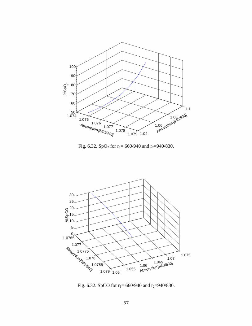
6.32 SpO2 for r1= 660/940 and r2=940/830 . 56
6.33 SpCO for r1= 660/940 and r2=940/830. 56
6.34 SpO2 for r1= 830/940 and r2=940/660 . 57
6.35 SpCO for r1= 830/940 and r2=940/660. 57
6.36 SpO2 for r1= 940/660 and r2=940/830 . 58
6.37 SpCO for r1= 940/660 and r2=940/830. 58
6.38 SpO2 for r1= 660/880 and r2=660/940 . 59
6.39 SpCO for r1= 660/880 and r2=660/940. 59
6.40 SpO2 for r1= 660/940 and r2=880/940 . 60
6.41 SpCO for r1= 660/940 and r2=880/940. 60
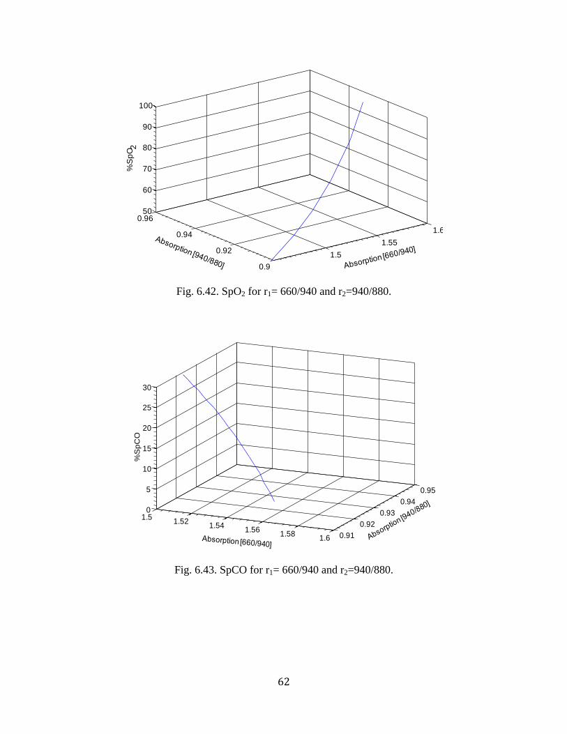
6.42 SpO2 for r1= 660/940 and r2=940/880 . 61
6.43 SpCO for r1= 660/940 and r2=940/880. 61
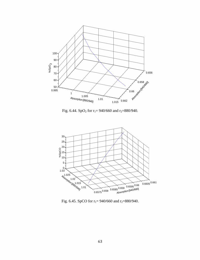
6.44 SpO2 for r1= 940/660 and r2=880/940 . 62
6.45 SpCO for r1= 940/660 and r2=880/940. 62
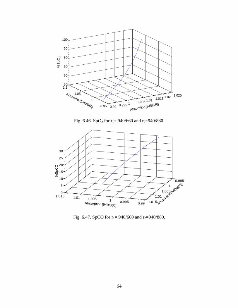
6.46 SpO2 for r1= 940/660 and r2=940/880 . 63
6.47 SpCO for r1= 940/660 and r2=940/880. 63
ix
6.48 SpO2 at r1= 660/940 and r2=660/610
for an average of six experiments. 67
6.49 SpCO at r1= 660/940 and r2=660/610
for an average of six experiments. 67
6.50 SpO2 at r1= 660/940 and r2=940/610
for an average of six experiments. 68
6.51 SpCO at r1= 660/940 and r2=940/610
for an average of six experiments. 68
6.52 SpO2 at r1= 660/940 and r2=610/940
for an average of six experiments. 69
6.53 SpCO at r1= 660/940 and r2=610/940
for an average of six experiments. 69
6.54 SpO2 at r1= 660/940 and r2=660/643
for an average of six experiments. 70
6.55 SpCO at r1= 660/940 and r2=660/643
for an average of six experiments. 70
6.56 SpO2 at r1= 660/940 and r2=643/940
for an average of six experiments. 71
6.57 SpCO at r1= 660/940 and r2=643/940
for an average of six experiments. 71
6.58 SpO2 at r1= 660/740 and r2=660/940
for an average of six experiments. 72
6.59 SpCO at r1= 660/740 and r2=660/940
for an average of six experiments. 72
6.60 SpO2 at r1=660/940 and r2=830/740
for an average of six experiments. 73
6.61 SpCO at r1=660/940 and r2=830/740
for an average of six experiments. 73
6.62 SpO2 at r1=660/940 and r2=660/830
for an average of six experiments. 74
x
6.63 SpCO at r1=660/940 and r2=660/830
for an average of six experiments. 74
6.64 SpO2 at r1=660/880 and r2=660/940
for an average of six experiments. 75
6.65 SpCO at r1=660/880 and r2=660/940
for an average of six experiments. 75
6.66 SpO2 at r1=660/940 and r2=880/940
for an average of six experiments. 76
6.67 SpCO at r1=660/940 and r2=880/940
for an average of six experiments. 76
8.1 Calculated SpO2 versus IL 682 HbO2 values. Dashed line is the line of
identity. Regression equation:
(Calculated SpO2)= 0.4 (IL-682 HbO2) + 50. 81
8.2 Calibrated SpO2 versus IL 682 HbO2 values. Dashed line is the line of
identity. Regression equation:
Calibrated SpO2=0.99*(IL-682 HbO2) +1.1. 81
8.3 Residual plot for data points shown in Fig. 8.2. 82
8.4 Calculated SpCO versus IL 682 HbCO values. Dashed line is the line
of identity. Regression equation:
(Calculated SpCO)= 0.6*(IL 682 HbCO) + 8.4. 82
8.5 Calibrated SpCO versus IL 682 HbCO values. Dashed line is the line
of identity. Regression equation:
(Calibrated SpCO) = (IL 682 HbCO) + 0.28). 83
8.6 Residual plot for data shown in Fig. 8.5. 83
xi
List of tables
Table Page
5.1 AC/DC ratios (mean ±standard deviation) for three sets of experiments with
varying SpO2. 25
5.2 AC/DC ratios (mean ±standard deviation) for three sets of experiments with
varying SpCO. 26
6.1 Theoretical models derived for different ratio 37
6.2 The wavelengths used categorised according to their sensitivity 65
7.1 Thresholds used in the algorithm to differentiate the presence and absence of
HbCO 79
8.1 Calculated SpCO corresponding to steady state HbCO at 26.3-27.1%
obtained at four different sensor positions. 85
8.2 Mean and standard deviation between the calculated values for SpCO
at different sensor positions. 85
8.3 Performance characteristics for %SpO2 measurements obtained from the
in-vitro model and our sensor using our algorithm 88
8.4 Performance characteristics for %SpCO measurements obtained from the
in-vitro model and our sensor using our algorithm. 89
8.5 Comparison of SpCO with HbCO measured by a CO-Oximeter 90
xii
List of abbreviations
Hb Hemoglobin
HbO2 Oxyhemoglobin
HbCO Carboxyhemoglobin
MetHb Methemoglobin
THb Total Hemoglobin
SpO2 Oxygen saturation
SpCO Carbon monoxide saturation
O2 Oxygen
CO Carbon monoxide
PPG Photoplethysmogram
AVF Armored fighting vehicle
LED Light emitting diode
1
Chapter 1. Physiological and clinical significance of oxygen and carbon monoxide
saturation
1.1. Oxygen saturation and its significance
Oxygen (O2) is essential to human life. Cells and tissues in the body require oxygen to survive.
Any reduction in the supply of this vital nutrient causes irreversible cell damage or even death.
O2 is not particularly soluble in blood [1]. Normally, only about 3% of the total oxygen carried is
in a dissolved state while about 97% of the oxygen transported to the tissues is carried by
hemoglobin (Hb). Therefore, Hb is solely responsible for the bulk of O2 transportation to tissues
[2].
Hb is an iron-containing protein that is made of amino acids strung together forming
polypeptide chains. Each hemoglobin molecule consists of a heme component and a globin
component. The globin unit is made up of four polypeptide chains. In commonly occurring
forms of adult Hb, two of the polypeptide chains are called alpha chains and the other two are
called beta chains. Each of these chains has one heme group which has an iron atom at the center
of a porphyrin ring. One polypeptide chain with a heme group is a subunit of Hb. Hb has four
such subunits, each with an iron atom [3]. These iron atoms in the heme group are the binding
sites for molecules. Each oxygen molecule combines with one iron atom loosely and reversibly.
Hence, four O2 molecules can bind to one molecule of Hb [4]. For one polypeptide chain the
reaction between Hb and O2 can be shown as
H O2 H O2 (1.1)
Hb with oxygen combined to it is called oxyhemoglobin (HbO2), while Hb without any oxygen
bound to it is called deoxyhemoglobin or reduced Hb (Hb). Normal human blood contains 15 g
Hb/ 100 ml blood. Each gram of Hb can bind with about 1.34 ml of O2 resulting in an oxygen
2
capacity of 20ml/100 ml of blood [5]. Oxygen saturation in blood is defined as the fraction of
Hb molecules that are bound to O2. Oxygen saturation can be defined in terms of functional
oxygen saturation or as fractional oxygen saturation. Fractional oxygen saturation is defined as
the ratio of HbO2 concentration to the total concentration of Hb. Functional oxygen saturation is
defined as the ratio of HbO2 concentration to the sum of the concentrations of Hb and HbO2.
Pulse oximeters measure functional oxygen saturation (SpO2) given by Eq. 1.2.
(1.2)
When the oxygen saturation is at 100%, there are no free binding sites available.
SpO2 measurement is commonly used in anesthesia, neonatology, pediatric care, cardio-
pulmonary resuscitations and intensive care. Using pulse oximeters, desaturation in anesthetized
patients can be identified in real time before irreversible tissue death occurs. It is especially
useful in preventing hypoxemia that occurs due to diminished alveolar ventilation during
anesthesia [6]. Pulse oximeters are also used as a standard diagnostic tool in intensive care and
emergency room.
1.2. Physiological and clinical effects of CO
The most important physiological effect of CO exposure is its preferential binding with Hb. The
binding affinity of CO is ~230 times the affinity O2 has for Hb. Hence, when CO exposure
occurs, Hb binds preferentially with CO resulting in the formation of carboxyhemoglobin
(HbCO) [7]. The effect of this preferential binding is the shift in the Hb dissociation curve to the
left (Fig. 1.1) [8].
3
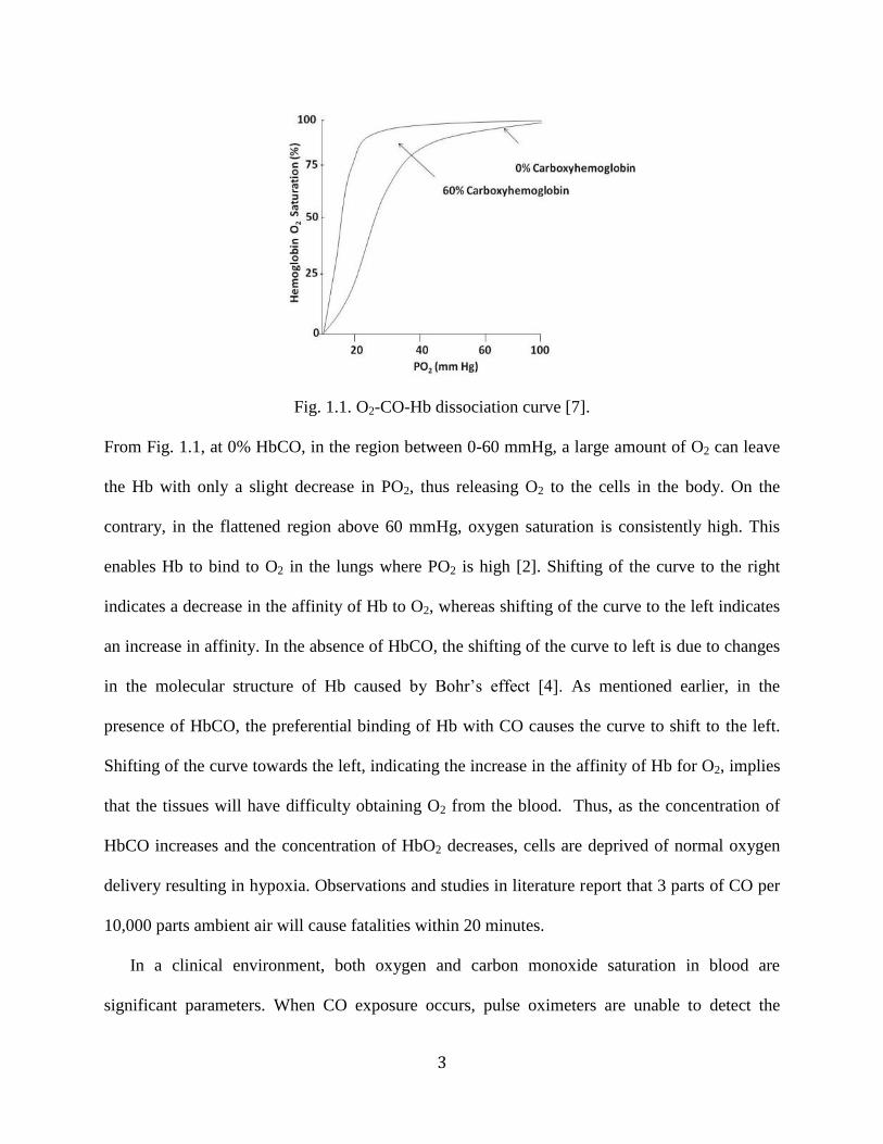
Fig. 1.1. O2-CO-Hb dissociation curve [7].
From Fig. 1.1, at 0% HbCO, in the region between 0-60 mmHg, a large amount of O2 can leave
the Hb with only a slight decrease in PO2, thus releasing O2 to the cells in the body. On the
contrary, in the flattened region above 60 mmHg, oxygen saturation is consistently high. This
enables Hb to bind to O2 in the lungs where PO2 is high [2]. Shifting of the curve to the right
indicates a decrease in the affinity of Hb to O2, whereas shifting of the curve to the left indicates
an increase in affinity. In the absence of HbCO, the shifting of the curve to left is due to changes
in the molecular structure of Hb caused y Bohr’s effect [4]. As mentioned earlier, in the
presence of HbCO, the preferential binding of Hb with CO causes the curve to shift to the left.
Shifting of the curve towards the left, indicating the increase in the affinity of Hb for O2, implies
that the tissues will have difficulty obtaining O2 from the blood. Thus, as the concentration of
HbCO increases and the concentration of HbO2 decreases, cells are deprived of normal oxygen
delivery resulting in hypoxia. Observations and studies in literature report that 3 parts of CO per
10,000 parts ambient air will cause fatalities within 20 minutes.
In a clinical environment, both oxygen and carbon monoxide saturation in blood are
significant parameters. When CO exposure occurs, pulse oximeters are unable to detect the
4
presence of HbCO and also lose the ability to measure SpO2 accurately. This is an important
limitation because CO, a colorless, odorless gas, is the leading cause of poisoning deaths in the
United States. It is believed to be responsible for more than half the poisoning deaths worldwide.
Around 5000 to 6000 people die every year in the United States alone due to CO exposure. CO
exposures at home or workplaces can occur due to improper maintenance of heaters, indoor air
conditioners, gas stoves, and vehicle exhaust. While firefighters are susceptible to CO poisoning
due to smoke inhalation, army field exposures commonly occur in tanks, troop compartments of
armored vehicles, enclosed communication vans, indoor testing and firing of weapons [7].
Miners are another group of people who are at the risk of CO poisoning. Several accidents
resulting in fatalities of miners have been reported due to CO exposure, caused by detonations
and explosions in the confines of a narrow shaft [8]. Due to lack of ventilation, the miners will be
exposed to high concentrations of CO in within a short span that results in fatalities. There have
also been reports of CO poisoning cases in houses constructed near old shaft mines [9].
Apparent health effects of CO exposure is reported to occur at a concentration of approximately
20% and higher. Early cardiovascular effect caused by CO poisoning is tachycardia in response
to hypoxia [10-11]. At higher concentrations hypotension, dysrhythmia, ischemia, infarction and
cases of cardiac arrest have been reported [7]. Therefore, diagnosing CO poisoning before it
causes severe tissue damage becomes critical. If pulse oximeters could monitor HbCO levels
noninvasively, patients with CO poisoning may be treated immediately, thus preventing further
harm. Also, in case of exposure during combat or fire, medics might be able to perform remote
triage from a safe location without being exposed to CO.
Diagnosing CO poisoning at early stages is the key because Hb-CO binding is a reversible
chemical reaction. After dissociating from CO, Hb does not exhibit any impairment in its oxygen

5
carrying capacity [12]. Hence, if patients who have been exposed to CO poisoning can be treated
immediately, damage to cells and tissues can be prevented.
6
Chapter 2. Background on pulse oximetry
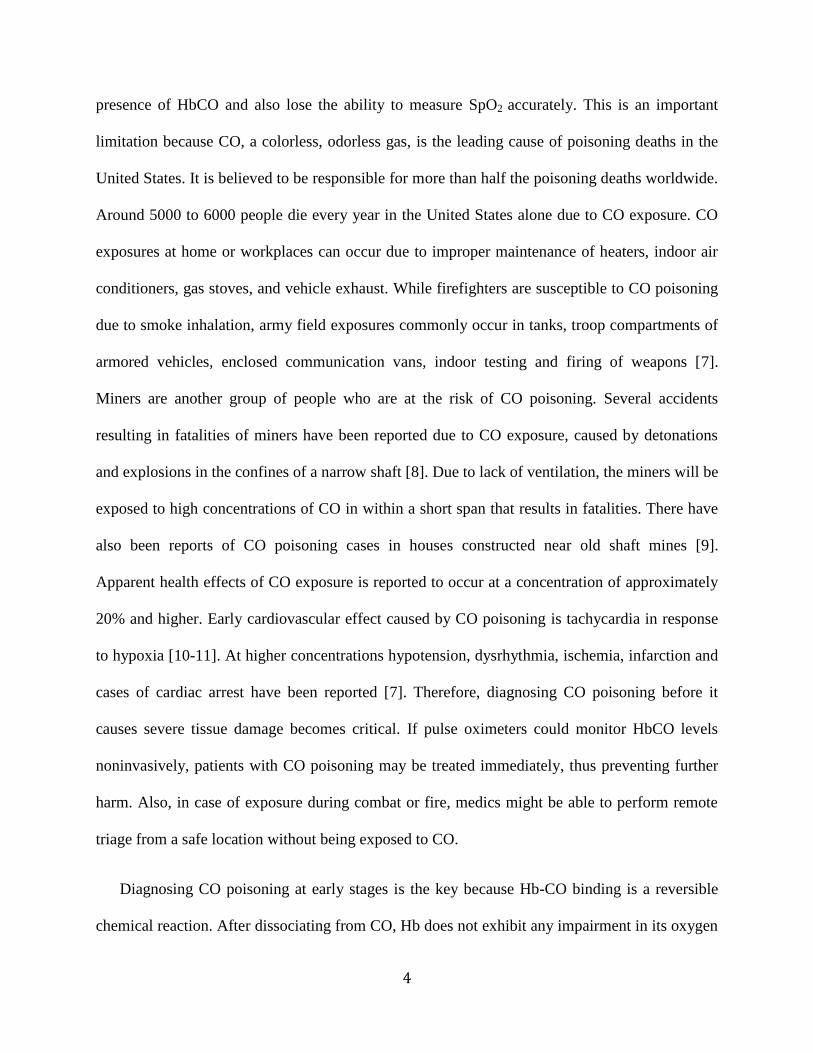
Pulse oximeters measure SpO2 in blood noninvasively using the time-varying
photoplethysmographic signal (PPG) caused by variation in the arterial blood volume
corresponding to the heart beat [13]. When light is passed through the skin, it is absorbed by
venous blood, tissue, hair, skin pigments, pulsating and non-pulsating arterial blood. During
systole, when there is more blood in the arteries, there is an increased absorption as the diameter
of the arteries increase. During diastole, when blood in the arteries is diminished, the light path
length is decreased and hence the absorption decreases. Thus, light absorption pulsates between
the maximum and minimum intensity, resulting in a PPG signal as illustrated in Fig. 2.1. The
absorption of light through the skin, hair and tissues is constant for a given individual and is
denoted as the DC component.
Fig. 2.1. Light absorption through the skin [13].
2.1. SpO2 measurement using pulse oximetry
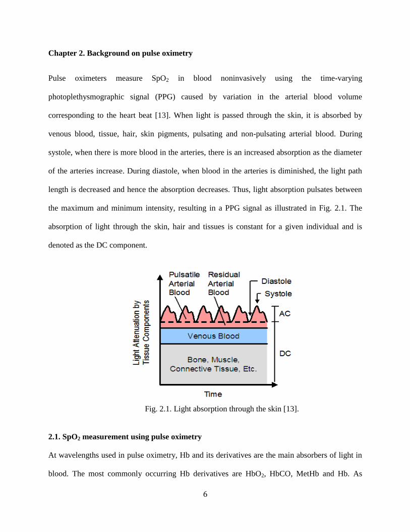
At wavelengths used in pulse oximetry, Hb and its derivatives are the main absorbers of light in
blood. The most commonly occurring Hb derivatives are HbO2, HbCO, MetHb and Hb. As
7
shown in Fig. 2.2, in the red region, the absorption of light by Hb is more than the absorption of
HbO2. Similarly, the absorption of light in the IR region is low for Hb compared to the
absorption caused by HbO2. Assuming that HbCO and MetHb are absent, SpO2 is measured
based on the variation in this absorption of light by HbO2 and Hb (Fig. 2.2). Two wavelengths,
typically from the red and infrared region, are used. The ratios of PPG signals at these two
wavelengths are used to calculate SpO2 [14].
Fig. 2.2. Absorption spectra of Hb and its derivatives [14].
SpO2 calculation is based on the assumption that HbCO and MetHb are absent. When HbCO
or MetHb is present in significant quantities, pulse oximeters give erroneous SpO2 readings.
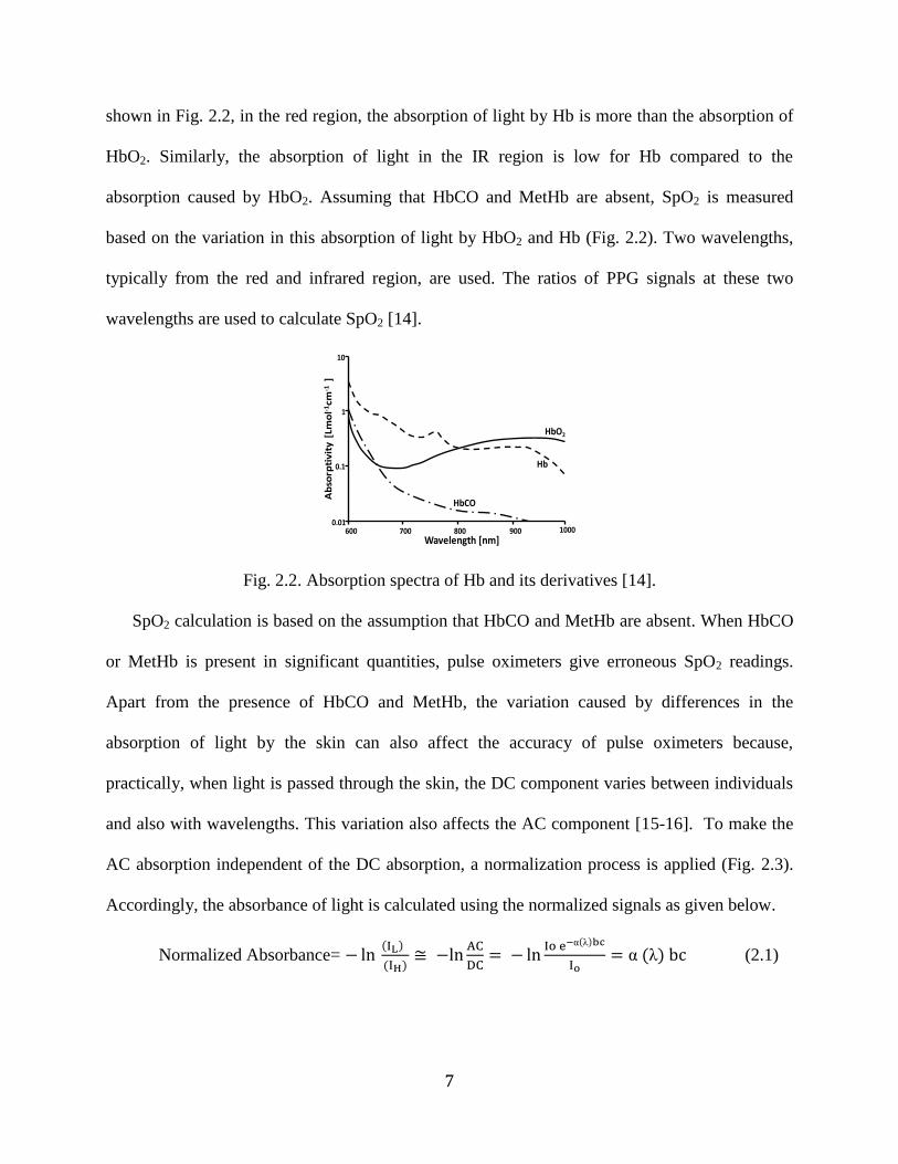
Apart from the presence of HbCO and MetHb, the variation caused by differences in the
absorption of light by the skin can also affect the accuracy of pulse oximeters because,
practically, when light is passed through the skin, the DC component varies between individuals
and also with wavelengths. This variation also affects the AC component [15-16]. To make the
AC absorption independent of the DC absorption, a normalization process is applied (Fig. 2.3).
Accordingly, the absorbance of light is calculated using the normalized signals as given below.
Normalized Absorbance= ( )
( )
( )
( ) (2.1)
10
1
0.1
0.01
Ab
sorp
tiv
ity
[Lm
ol-1
cm-1
]
Wavelength [nm]600 800 900 1000700
HbCO
Hb
HbO2
8
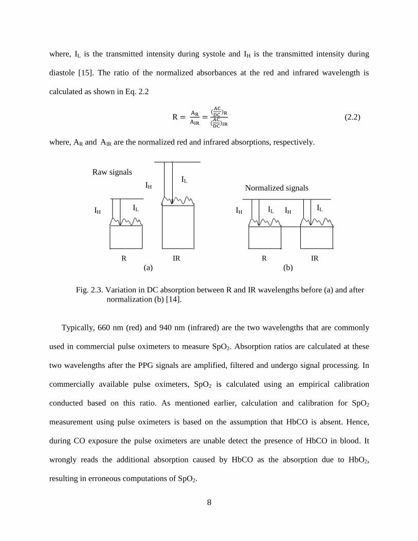
where, IL is the transmitted intensity during systole and IH is the transmitted intensity during
diastole [15]. The ratio of the normalized absorbances at the red and infrared wavelength is
calculated as shown in Eq. 2.2
(
)
(
)
(2.2)
where, AR and AIR are the normalized red and infrared absorptions, respectively.
Fig. 2.3. Variation in DC absorption between R and IR wavelengths before (a) and after
normalization (b) [14].
Typically, 660 nm (red) and 940 nm (infrared) are the two wavelengths that are commonly
used in commercial pulse oximeters to measure SpO2. Absorption ratios are calculated at these
two wavelengths after the PPG signals are amplified, filtered and undergo signal processing. In
commercially available pulse oximeters, SpO2 is calculated using an empirical calibration
conducted based on this ratio. As mentioned earlier, calculation and calibration for SpO2
measurement using pulse oximeters is based on the assumption that HbCO is absent. Hence,
during CO exposure the pulse oximeters are unable detect the presence of HbCO in blood. It
wrongly reads the additional absorption caused by HbCO as the absorption due to HbO2,
resulting in erroneous computations of SpO2.
IH
IL
IH IL
IH IL
Normalized signals
Raw signals
IH
IL
(b) (a)
R IR R IR
9
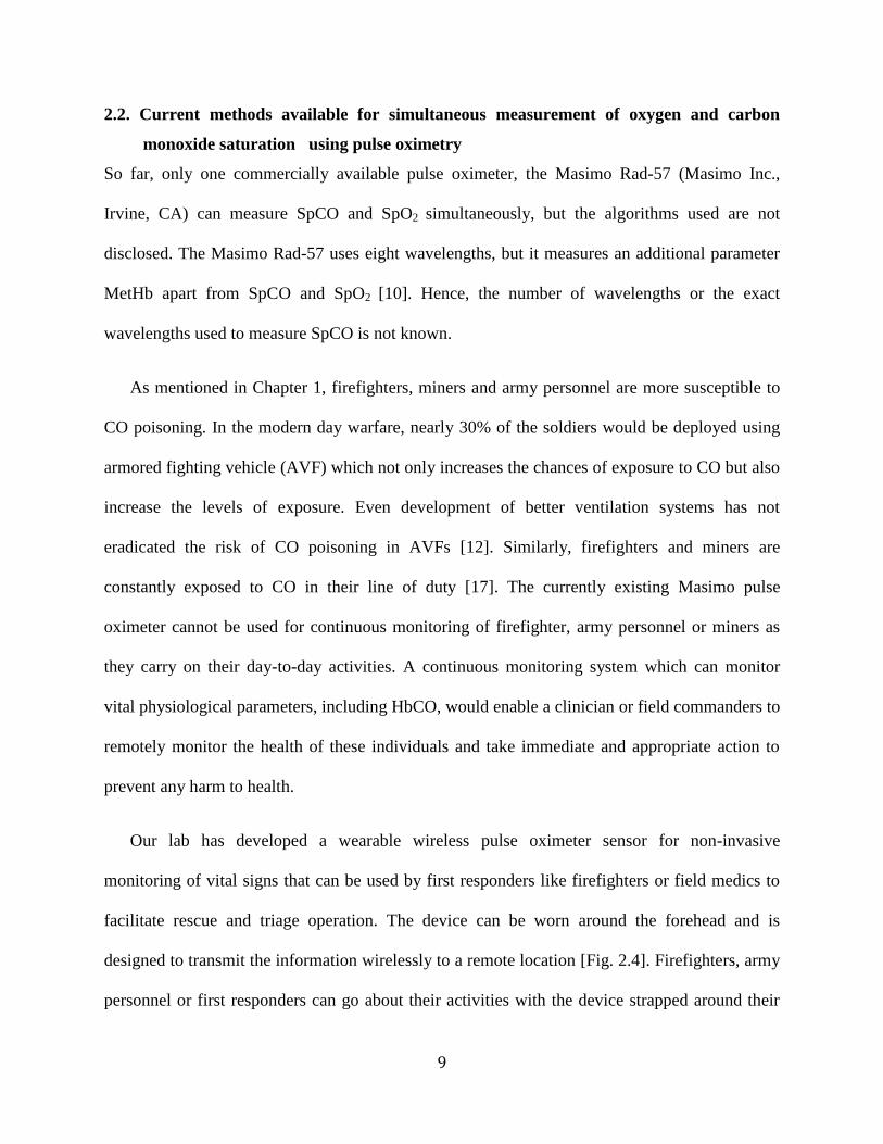
2.2. Current methods available for simultaneous measurement of oxygen and carbon
monoxide saturation using pulse oximetry
So far, only one commercially available pulse oximeter, the Masimo Rad-57 (Masimo Inc.,
Irvine, CA) can measure SpCO and SpO2 simultaneously, but the algorithms used are not
disclosed. The Masimo Rad-57 uses eight wavelengths, but it measures an additional parameter
MetHb apart from SpCO and SpO2 [10]. Hence, the number of wavelengths or the exact
wavelengths used to measure SpCO is not known.
As mentioned in Chapter 1, firefighters, miners and army personnel are more susceptible to
CO poisoning. In the modern day warfare, nearly 30% of the soldiers would be deployed using
armored fighting vehicle (AVF) which not only increases the chances of exposure to CO but also
increase the levels of exposure. Even development of better ventilation systems has not
eradicated the risk of CO poisoning in AVFs [12]. Similarly, firefighters and miners are
constantly exposed to CO in their line of duty [17]. The currently existing Masimo pulse
oximeter cannot be used for continuous monitoring of firefighter, army personnel or miners as
they carry on their day-to-day activities. A continuous monitoring system which can monitor
vital physiological parameters, including HbCO, would enable a clinician or field commanders to
remotely monitor the health of these individuals and take immediate and appropriate action to
prevent any harm to health.
Our lab has developed a wearable wireless pulse oximeter sensor for non-invasive
monitoring of vital signs that can be used by first responders like firefighters or field medics to
facilitate rescue and triage operation. The device can be worn around the forehead and is
designed to transmit the information wirelessly to a remote location [Fig. 2.4]. Firefighters, army
personnel or first responders can go about their activities with the device strapped around their
10
forehead. The wireless pulse oximeter sensor developed in our laboratory can measure SpO2,
heart rate (HR) and respiratory rate (RR). The aim of this thesis was to develop an algorithm that
can be used in this wireless device to simultaneously measure SpO2 and carbon monoxide
saturation (SpCO).
Fig. 2.4. Multiwavelength wireless pulse oximeter device designed in our lab.
Inadequacies of commercial pulse oximeters like low battery life, bulkiness and wires that
prohibit the use of the device in field applications have been eliminated in our wireless pulse
oximeter. Hence, if the wireless device can simultaneously measure SpO2 and SpCO, it will find
additional potential applications not just for firefighters or first responders, but also in clinical
settings where patient mobility is important.
11
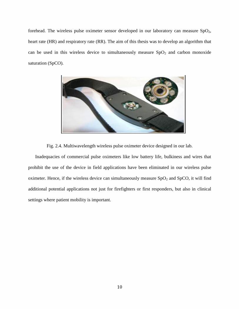
Chapter 3: Specific objectives
The inability of pulse oximeters to measure HbCO in blood, or measure accurate values of SpO2
in the presence of elevated levels of HbCO, is an important limitation because high exposure to
CO can be fatal or result in permanent neurological damage. If pulse oximeters could monitor
HbCO levels, CO poisoning can be treated immediately, preventing further harm. Therefore, the
aim of this thesis was to develop an algorithm that could simultaneously measure SpO2 and
HbCO in blood using a pulse oximeter. The specific objectives of this thesis were to:
1. Develop a theoretical model for simultaneous measurement of SpCO and SpO2.
2. Identify the specific wavelengths at which changes in SpCO and SpO2 can be measured
simultaneously.
3. Formulate an algorithm to simultaneously measure SpCO and SpO2 using pulse oximetry.
4. Verify the algorithm experimentally using an in-vitro set up.
12
Chapter 4. In-vitro model for simultaneous measurement of SpO2 and SpCO
4.1. Need for an in-vitro model
Although in-vivo measurements can provide information on the impact of different physiological
variables, it is not practically possible to desaturate a healthy individual below 80% or elevate
SpCO above 12% due to safety and ethical considerations as there is a risk of hypoxic brain
damage to the person at SpO2 values lower than 80% and greater than 12% SpCO. Hence, it is
difficult to obtain data from in-vivo measurements at low values of SpO2 or high values of SpCO
for initial testing of pulse oximeters [16]. Use of animal models for initial testing of pulse
oximeters is possible. But, results from animal studies have suggested that unknown or
uncontrollable physiological parameters can cause large variation especially at low SpO2 values
[18]. Similarly, a study comparing an animal model and in-vivo calibration reports that
differences in skin structure between humans and animals can also affect the calibration of pulse
oximeter. Although, piglets are reported to have histologically a skin structure similar to human
beings, the effect of skin structure on pulse oximeters has not been completely studied [18].
Hence, in spite of calibration using animal models, as mentioned in chapter 2, pulse oximeters
have to be finally calibrated on humans. This is because there is no other accepted standard
reference for checking the calibration of pulse oximeter [20]. As shown in Fig. 4.1, in-vivo
calibration for SpO2 requires in-vivo tests on volunteers after they breathe N2 gas to decrease the
SpO2 in their blood. Similarly, SpCO calibration required subject to breathe CO to elevate the
concentration of HbCO in the blood. These studies are expensive, time consuming and carry a
certain risk. Hence, in-vitro measurements using a tissue simulator can be a practical and
relatively inexpensive method for initial testing and calibration of a new pulse oximeter.
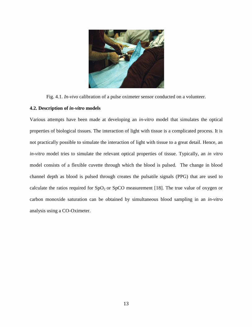
13
Fig. 4.1. In-vivo calibration of a pulse oximeter sensor conducted on a volunteer.
4.2. Description of in-vitro models
Various attempts have been made at developing an in-vitro model that simulates the optical
properties of biological tissues. The interaction of light with tissue is a complicated process. It is
not practically possible to simulate the interaction of light with tissue to a great detail. Hence, an
in-vitro model tries to simulate the relevant optical properties of tissue. Typically, an in vitro
model consists of a flexible cuvette through which the blood is pulsed. The change in blood
channel depth as blood is pulsed through creates the pulsatile signals (PPG) that are used to
calculate the ratios required for SpO2 or SpCO measurement [18]. The true value of oxygen or
carbon monoxide saturation can be obtained by simultaneous blood sampling in an in-vitro
analysis using a CO-Oximeter.
14
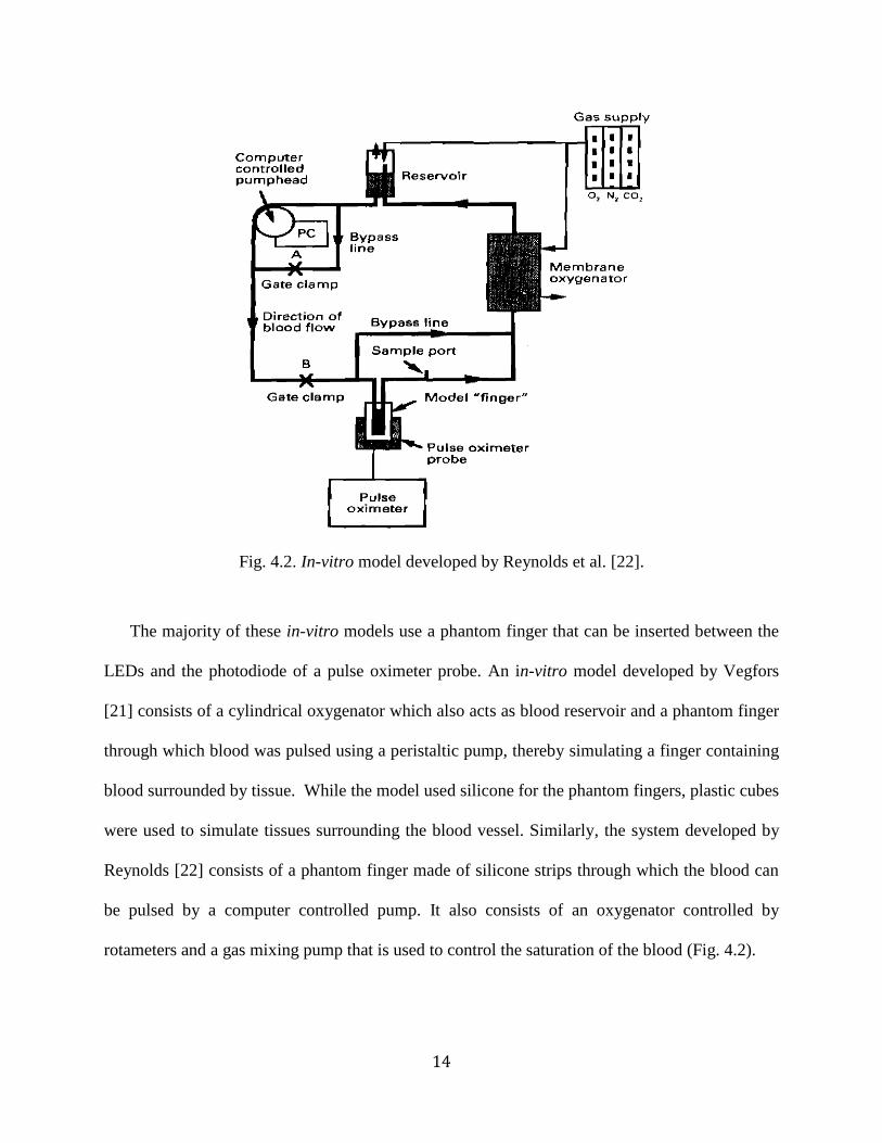
Fig. 4.2. In-vitro model developed by Reynolds et al. [22].
The majority of these in-vitro models use a phantom finger that can be inserted between the
LEDs and the photodiode of a pulse oximeter probe. An in-vitro model developed by Vegfors
[21] consists of a cylindrical oxygenator which also acts as blood reservoir and a phantom finger
through which blood was pulsed using a peristaltic pump, thereby simulating a finger containing
blood surrounded by tissue. While the model used silicone for the phantom fingers, plastic cubes
were used to simulate tissues surrounding the blood vessel. Similarly, the system developed by
Reynolds [22] consists of a phantom finger made of silicone strips through which the blood can
be pulsed by a computer controlled pump. It also consists of an oxygenator controlled by
rotameters and a gas mixing pump that is used to control the saturation of the blood (Fig. 4.2).
15
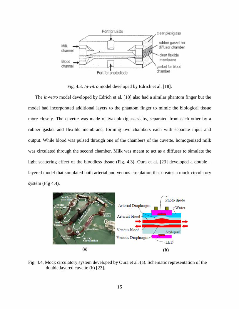
Fig. 4.3. In-vitro model developed by Edrich et al. [18].
The in-vitro model developed by Edrich et al. [18] also had a similar phantom finger but the
model had incorporated additional layers to the phantom finger to mimic the biological tissue
more closely. The cuvette was made of two plexiglass slabs, separated from each other by a
rubber gasket and flexible membrane, forming two chambers each with separate input and
output. While blood was pulsed through one of the chambers of the cuvette, homogenized milk
was circulated through the second chamber. Milk was meant to act as a diffuser to simulate the
light scattering effect of the bloodless tissue (Fig. 4.3). Oura et al. [23] developed a double –
layered model that simulated both arterial and venous circulation that creates a mock circulatory
system (Fig 4.4).
Fig. 4.4. Mock circulatory system developed by Oura et al. (a). Schematic representation of the
double layered cuvette (b) [23].
(a)
(b)
16
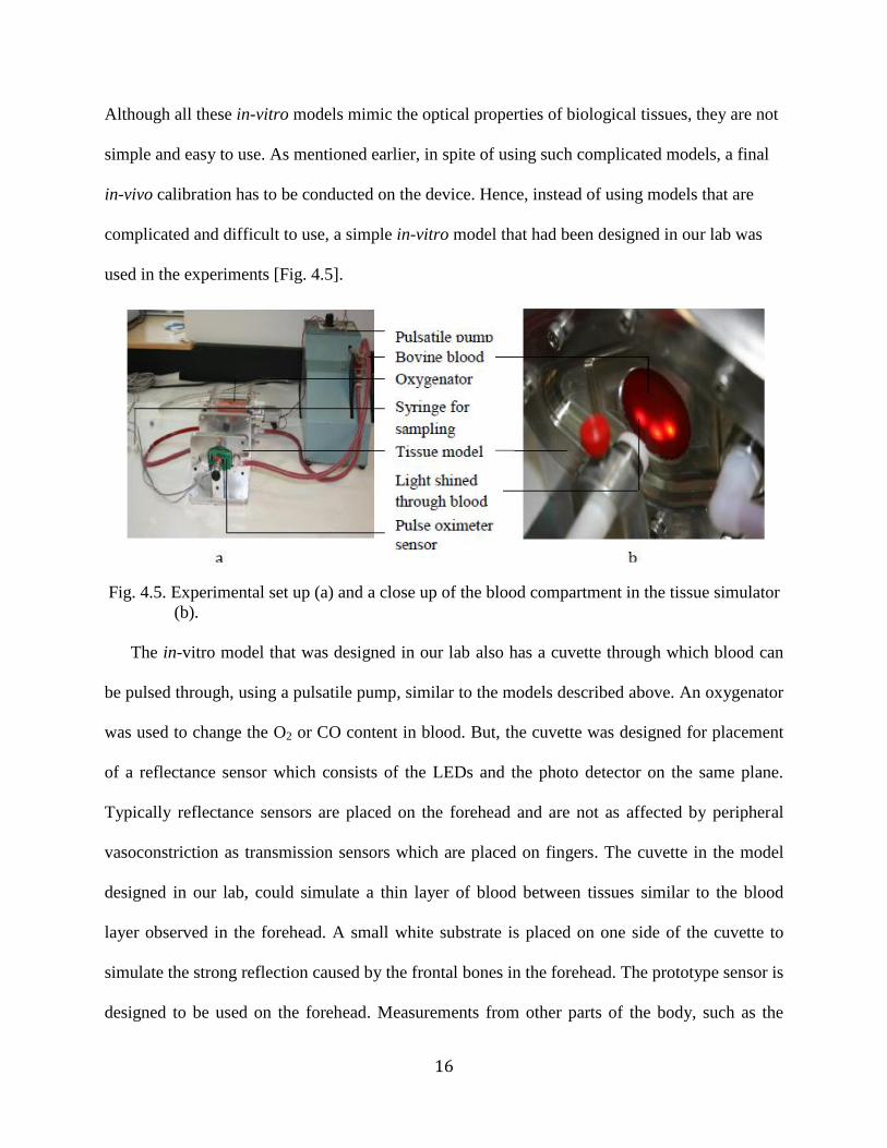
Although all these in-vitro models mimic the optical properties of biological tissues, they are not
simple and easy to use. As mentioned earlier, in spite of using such complicated models, a final
in-vivo calibration has to be conducted on the device. Hence, instead of using models that are
complicated and difficult to use, a simple in-vitro model that had been designed in our lab was
used in the experiments [Fig. 4.5].
Fig. 4.5. Experimental set up (a) and a close up of the blood compartment in the tissue simulator
(b).
The in-vitro model that was designed in our lab also has a cuvette through which blood can
be pulsed through, using a pulsatile pump, similar to the models described above. An oxygenator
was used to change the O2 or CO content in blood. But, the cuvette was designed for placement
of a reflectance sensor which consists of the LEDs and the photo detector on the same plane.
Typically reflectance sensors are placed on the forehead and are not as affected by peripheral
vasoconstriction as transmission sensors which are placed on fingers. The cuvette in the model
designed in our lab, could simulate a thin layer of blood between tissues similar to the blood
layer observed in the forehead. A small white substrate is placed on one side of the cuvette to
simulate the strong reflection caused by the frontal bones in the forehead. The prototype sensor is
designed to be used on the forehead. Measurements from other parts of the body, such as the
17
arms or legs are feasible, but typically result in poor signal-to-noise ratio because tissue depth in
these parts will cause high attenuation which in turn results in poor quality PPG signal.
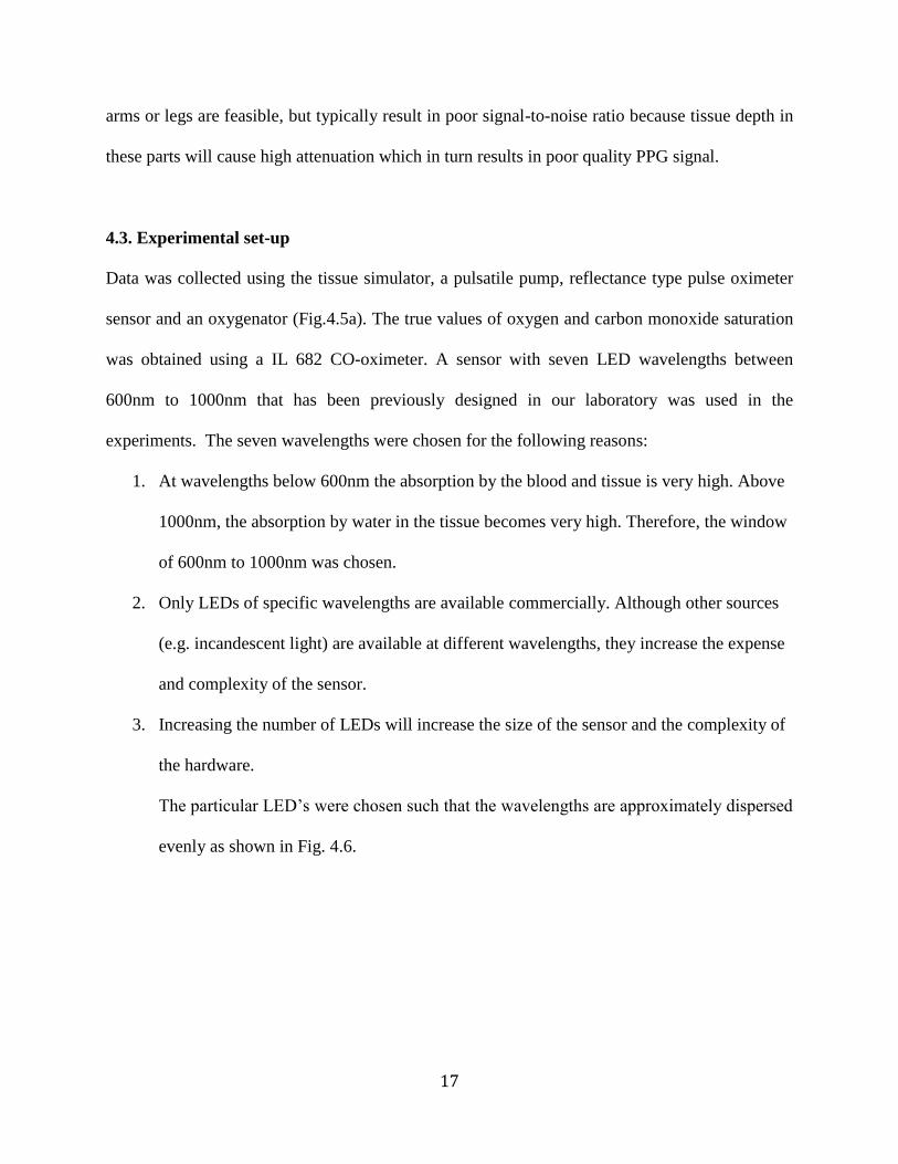
4.3. Experimental set-up
Data was collected using the tissue simulator, a pulsatile pump, reflectance type pulse oximeter
sensor and an oxygenator (Fig.4.5a). The true values of oxygen and carbon monoxide saturation
was obtained using a IL 682 CO-oximeter. A sensor with seven LED wavelengths between
600nm to 1000nm that has been previously designed in our laboratory was used in the
experiments. The seven wavelengths were chosen for the following reasons:
1. At wavelengths below 600nm the absorption by the blood and tissue is very high. Above
1000nm, the absorption by water in the tissue becomes very high. Therefore, the window
of 600nm to 1000nm was chosen.
2. Only LEDs of specific wavelengths are available commercially. Although other sources
(e.g. incandescent light) are available at different wavelengths, they increase the expense
and complexity of the sensor.
3. Increasing the number of LEDs will increase the size of the sensor and the complexity of
the hardware.
The particular LED’s were chosen such that the wavelengths are approximately dispersed
evenly as shown in Fig. 4.6.
18
Fig. 4.6. Absorption spectra for Hb and its derivatives. The vertical lines indicate
seven wavelengths used in our prototype sensor.
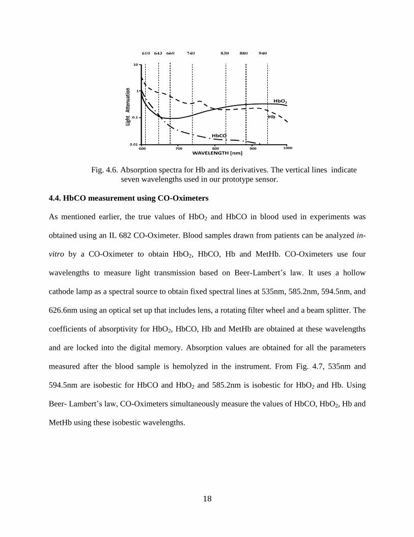
4.4. HbCO measurement using CO-Oximeters
As mentioned earlier, the true values of HbO2 and HbCO in blood used in experiments was
obtained using an IL 682 CO-Oximeter. Blood samples drawn from patients can be analyzed in-
vitro by a CO-Oximeter to obtain HbO2, HbCO, Hb and MetHb. CO-Oximeters use four
wavelengths to measure light transmission based on Beer-Lam ert’s law. It uses a hollow
cathode lamp as a spectral source to obtain fixed spectral lines at 535nm, 585.2nm, 594.5nm, and
626.6nm using an optical set up that includes lens, a rotating filter wheel and a beam splitter. The
coefficients of absorptivity for HbO2, HbCO, Hb and MetHb are obtained at these wavelengths
and are locked into the digital memory. Absorption values are obtained for all the parameters
measured after the blood sample is hemolyzed in the instrument. From Fig. 4.7, 535nm and
594.5nm are isobestic for HbCO and HbO2 and 585.2nm is isobestic for HbO2 and Hb. Using
Beer- Lam ert’s law, CO-Oximeters simultaneously measure the values of HbCO, HbO2, Hb and
MetHb using these isobestic wavelengths.
19
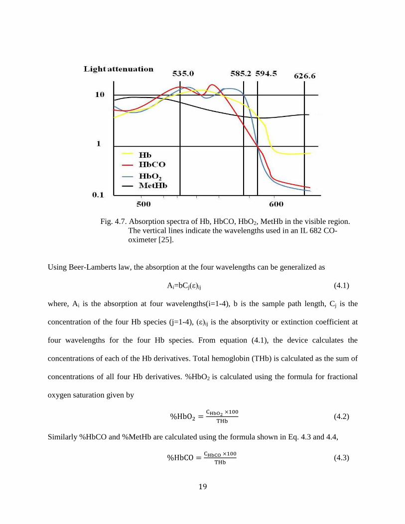
Fig. 4.7. Absorption spectra of Hb, HbCO, HbO2, MetHb in the visible region.
The vertical lines indicate the wavelengths used in an IL 682 CO-
oximeter [25].
Using Beer-Lamberts law, the absorption at the four wavelengths can be generalized as
Ai=bCj(ε)ij (4.1)
where, Ai is the absorption at four wavelengths(i=1-4), b is the sample path length, Cj is the
concentration of the four Hb species (j=1-4), (ε)ij is the absorptivity or extinction coefficient at
four wavelengths for the four Hb species. From equation (4.1), the device calculates the
concentrations of each of the Hb derivatives. Total hemoglobin (THb) is calculated as the sum of
concentrations of all four Hb derivatives. %HbO2 is calculated using the formula for fractional
oxygen saturation given by
(4.2)
Similarly %HbCO and %MetHb are calculated using the formula shown in Eq. 4.3 and 4.4,
(4.3)
20
(4.4)
A microcomputer is used to compute HbO2, HbCO, Hb and MetHb. The device has an accuracy
of 1% for all the parameters it measures [24]. The wavelengths used in CO-Oximetry are in the
visible range (500nm-650nm) where absorption by blood is very high (Fig. 4.7). The same
wavelengths cannot be used in pulse oximeters because the incident light absorbed by the tissue
and the thickness of blood in the tissues is high in the visible region.
21
Chapter 5: Preliminary research to validate the sensor and in-vitro model
Preliminary experiments were conducted to validate the data collected from our in-vitro model.
The goals of the preliminary experiments were to verify if the optical properties of blood, with
varying HbO2 and HbCO, observed from our sensor and model follow the trend suggested by the
standard absorption plot obtained using the coefficients of absorptivities derived from
spectrophotometric measurements on human blood as published in the literature [25]. For testing,
the pulse oximeter probe was attached to the model and HbO2 or HbCO concentrations were
varied by varying the amount of N2 or CO gas introduced into the set up, respectively. Readings
from the pulse oximeter were simultaneously obtained with blood sampled using an IL 682 CO-
Oximeter as a reference. The in-vitro testing was repeated at different concentrations of SpO2
and SpCO.
5.1. Methodology
5.1.1. SpO2 experiments
Since HbO2 in the blood varies according to variation in HbCO, understanding and verifying the
optical properties of blood with varying concentrations of HbO2 was necessary. HbO2
concentrations in the blood were varied from 50-100% and the absorption readings
corresponding to different concentrations were obtained at all wavelengths from the sensor.
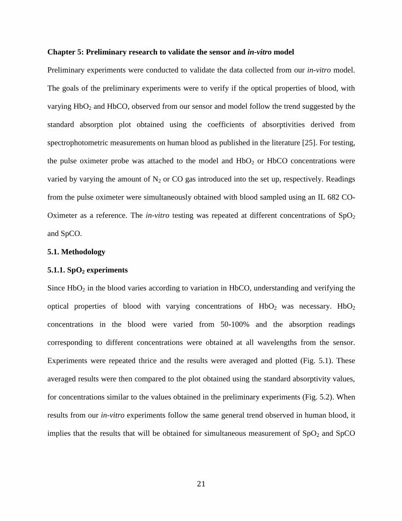
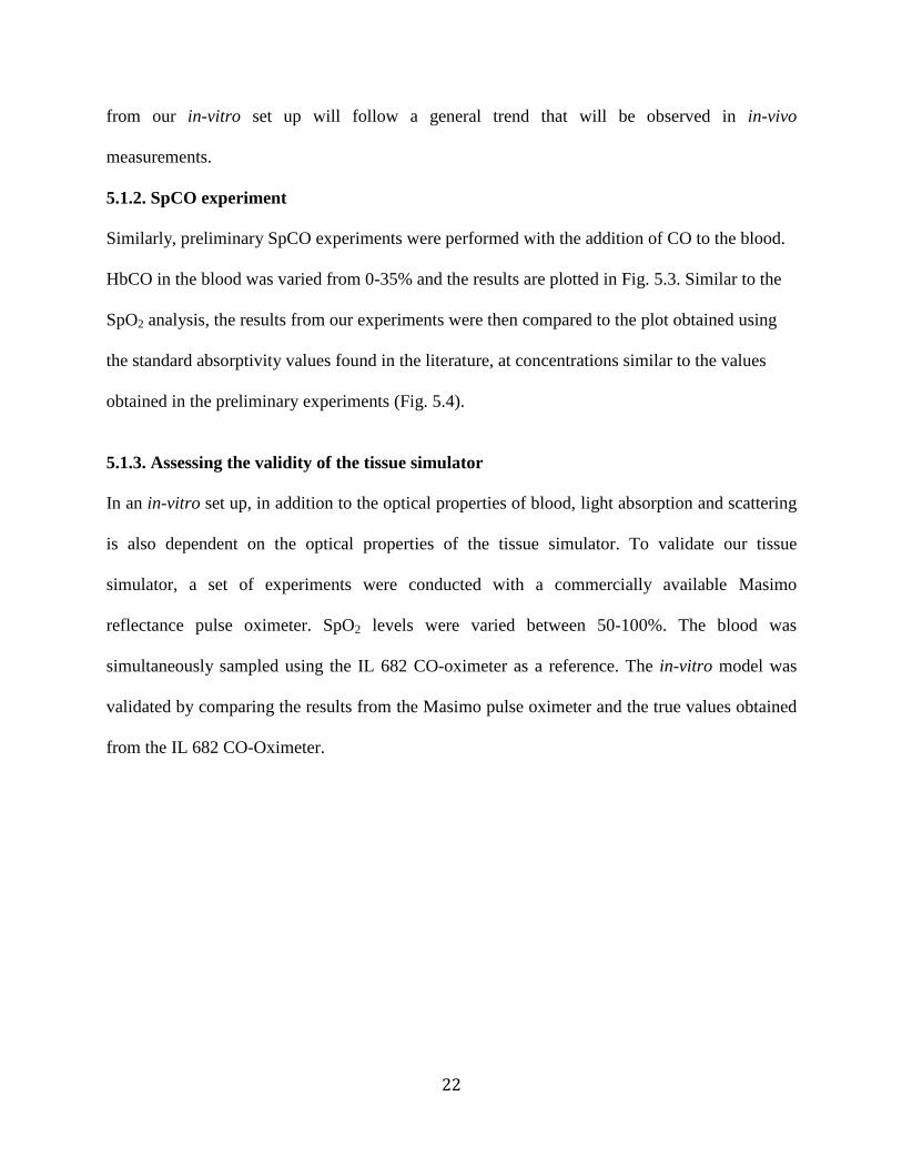
Experiments were repeated thrice and the results were averaged and plotted (Fig. 5.1). These
averaged results were then compared to the plot obtained using the standard absorptivity values,
for concentrations similar to the values obtained in the preliminary experiments (Fig. 5.2). When
results from our in-vitro experiments follow the same general trend observed in human blood, it
implies that the results that will be obtained for simultaneous measurement of SpO2 and SpCO
22
from our in-vitro set up will follow a general trend that will be observed in in-vivo
measurements.
5.1.2. SpCO experiment
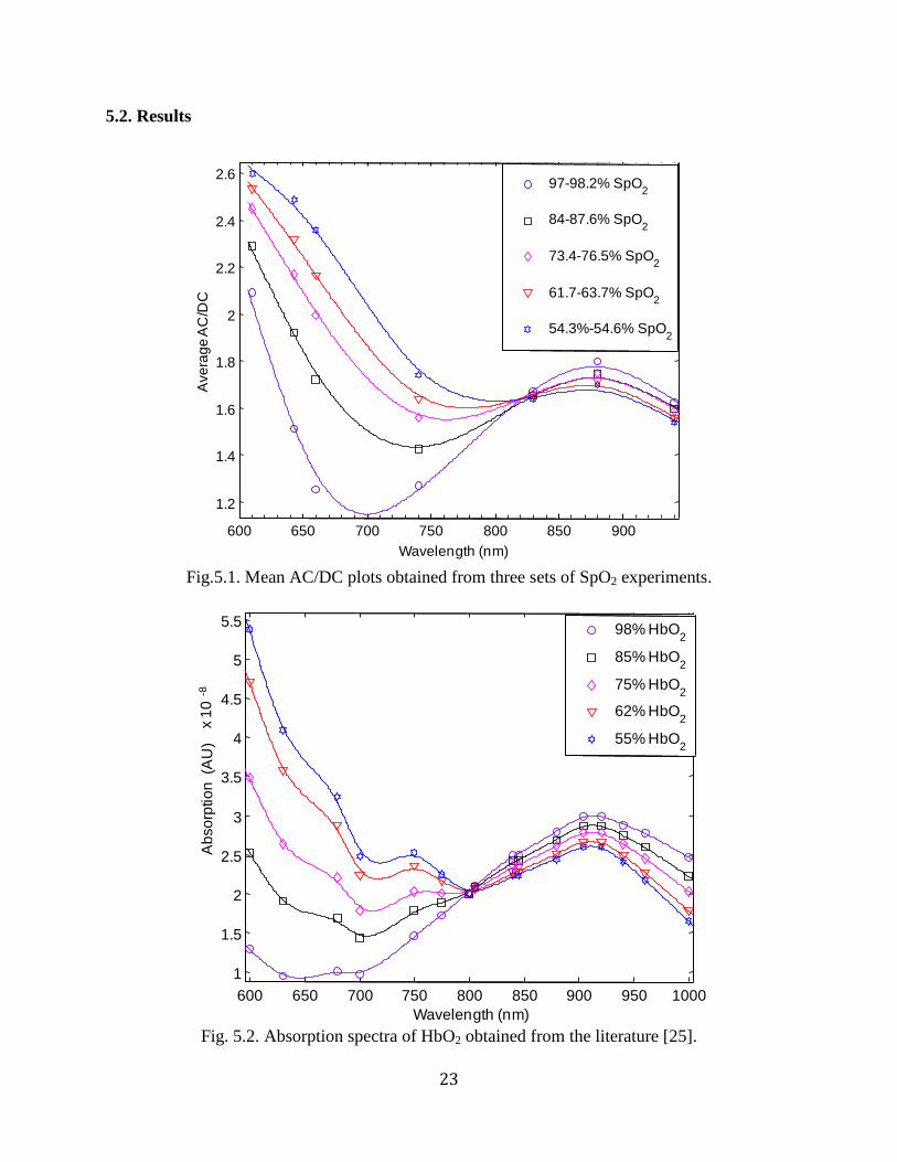
Similarly, preliminary SpCO experiments were performed with the addition of CO to the blood.
HbCO in the blood was varied from 0-35% and the results are plotted in Fig. 5.3. Similar to the
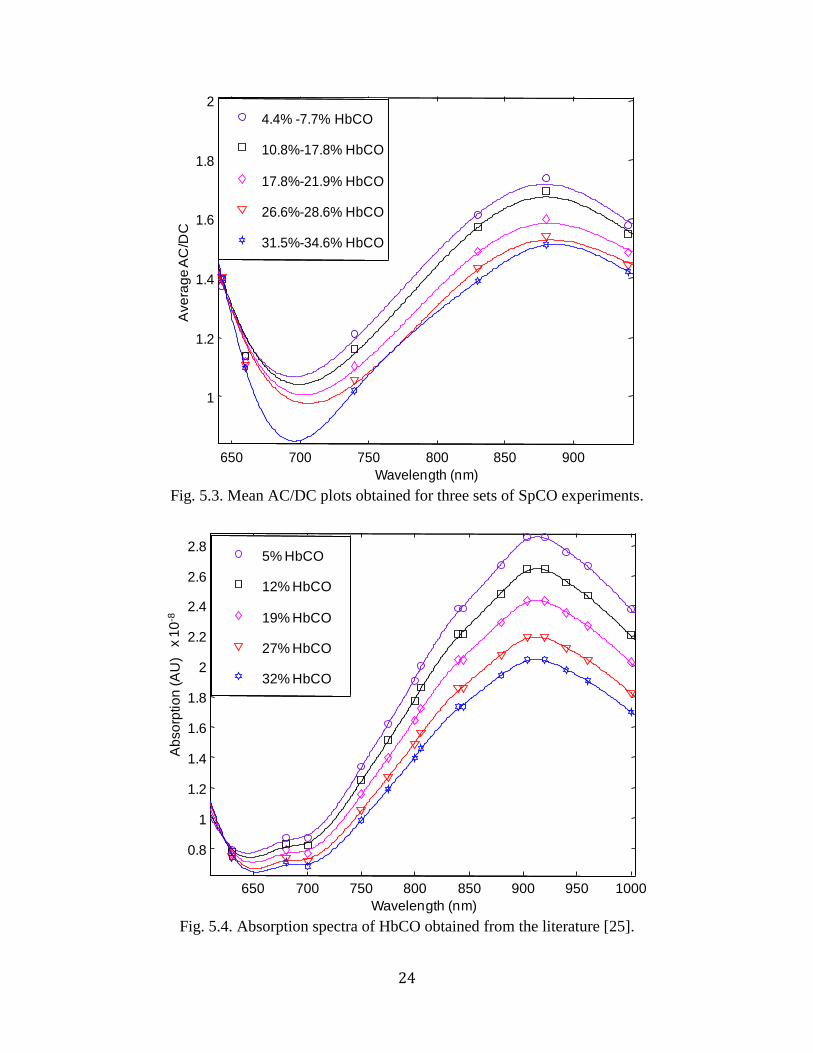
SpO2 analysis, the results from our experiments were then compared to the plot obtained using
the standard absorptivity values found in the literature, at concentrations similar to the values
obtained in the preliminary experiments (Fig. 5.4).
5.1.3. Assessing the validity of the tissue simulator
In an in-vitro set up, in addition to the optical properties of blood, light absorption and scattering
is also dependent on the optical properties of the tissue simulator. To validate our tissue
simulator, a set of experiments were conducted with a commercially available Masimo
reflectance pulse oximeter. SpO2 levels were varied between 50-100%. The blood was
simultaneously sampled using the IL 682 CO-oximeter as a reference. The in-vitro model was
validated by comparing the results from the Masimo pulse oximeter and the true values obtained
from the IL 682 CO-Oximeter.
23
5.2. Results
Fig.5.1. Mean AC/DC plots obtained from three sets of SpO2 experiments.
Fig. 5.2. Absorption spectra of HbO2 obtained from the literature [25].
600 650 700 750 800 850 900
1.2
1.4
1.6
1.8
2
2.2
2.4
2.6
Wavelength (nm)
Ave
rag
e A
C/D
C
97-98.2% SpO2
84-87.6% SpO2
73.4-76.5% SpO2
61.7-63.7% SpO2
54.3%-54.6% SpO2
600 650 700 750 800 850 900 950 1000
1
1.5
2
2.5
3
3.5
4
4.5
5
5.5
x 1
0 -8
Wavelength (nm)
Ab
so
rptio
n (
AU
)
98% HbO2
85% HbO2
75% HbO2
62% HbO2
55% HbO2
24
Fig. 5.3. Mean AC/DC plots obtained for three sets of SpCO experiments.
Fig. 5.4. Absorption spectra of HbCO obtained from the literature [25].
650 700 750 800 850 900
1
1.2
1.4
1.6
1.8
2
Wavelength (nm)
Ave
rag
e A
C/D
C
4.4% -7.7% HbCO
10.8%-17.8% HbCO
17.8%-21.9% HbCO
26.6%-28.6% HbCO
31.5%-34.6% HbCO
650 700 750 800 850 900 950 1000
0.8
1
1.2
1.4
1.6
1.8
2
2.2
2.4
2.6
2.8
x 1
0-8
Wavelength (nm)
Ab
so
rptio
n (A
U)
5% HbCO
12% HbCO
19% HbCO
27% HbCO
32% HbCO
25
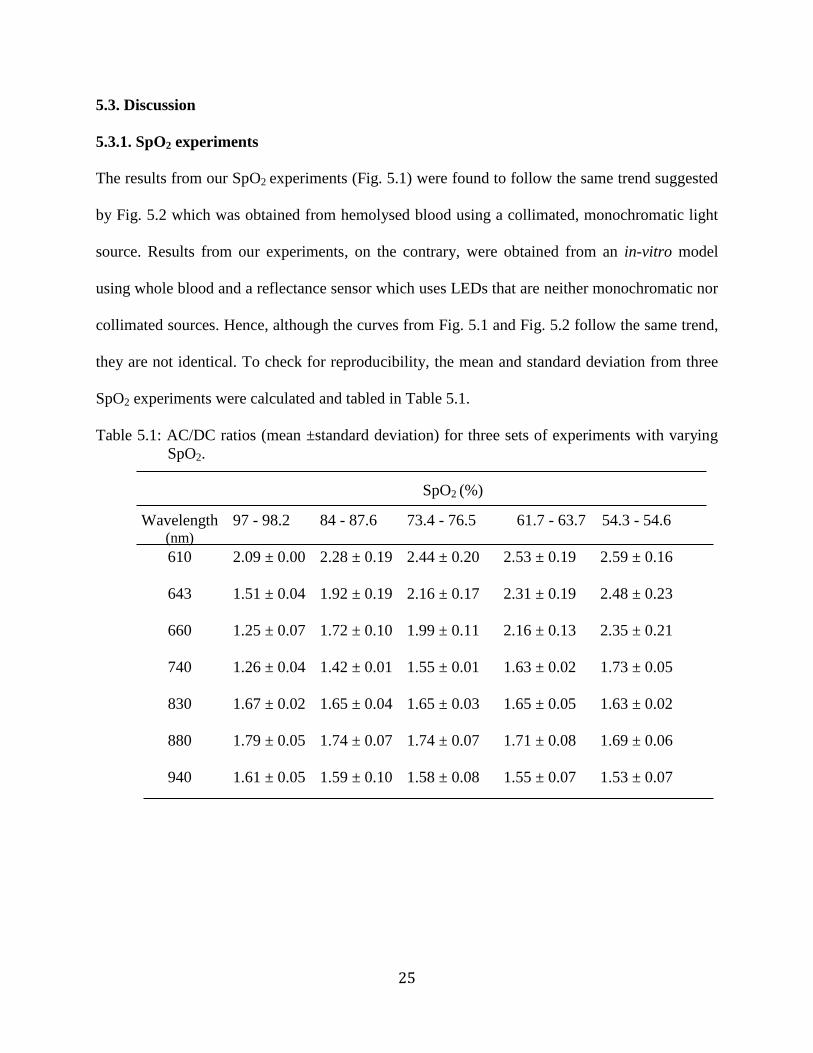
5.3. Discussion
5.3.1. SpO2 experiments
The results from our SpO2 experiments (Fig. 5.1) were found to follow the same trend suggested
by Fig. 5.2 which was obtained from hemolysed blood using a collimated, monochromatic light
source. Results from our experiments, on the contrary, were obtained from an in-vitro model
using whole blood and a reflectance sensor which uses LEDs that are neither monochromatic nor
collimated sources. Hence, although the curves from Fig. 5.1 and Fig. 5.2 follow the same trend,
they are not identical. To check for reproducibility, the mean and standard deviation from three
SpO2 experiments were calculated and tabled in Table 5.1.
Table 5.1: AC/DC ratios (mean ±standard deviation) for three sets of experiments with varying
SpO2.
SpO2 (%)
Wavelength (nm)
97 - 98.2 84 - 87.6 73.4 - 76.5
61.7 - 63.7
54.3 - 54.6
610 2.09 ± 0.00
2.28 ± 0.19 2.44 ± 0.20 2.53 ± 0.19 2.59 ± 0.16
643 1.51 ± 0.04
1.92 ± 0.19 2.16 ± 0.17 2.31 ± 0.19 2.48 ± 0.23
660 1.25 ± 0.07 1.72 ± 0.10 1.99 ± 0.11 2.16 ± 0.13 2.35 ± 0.21
740 1.26 ± 0.04
1.42 ± 0.01 1.55 ± 0.01 1.63 ± 0.02 1.73 ± 0.05
830 1.67 ± 0.02 1.65 ± 0.04 1.65 ± 0.03 1.65 ± 0.05 1.63 ± 0.02
880 1.79 ± 0.05 1.74 ± 0.07 1.74 ± 0.07 1.71 ± 0.08 1.69 ± 0.06
940 1.61 ± 0.05 1.59 ± 0.10 1.58 ± 0.08 1.55 ± 0.07 1.53 ± 0.07
26
From Table 5.1, at 610 nm, 643 nm and 660 nm, the absorption by Hb is high for lower values of
SpO2. This results in a weak signal, thereby, decreasing the signal-to-noise ratio. Hence, the
variation is higher for low values of SpO2 but low at higher ranges of SpO2. Since the variation
between the three sets of readings is less than 1% for all the ranges of SpO2 and wavelength
tested, the results obtained using our sensor and in-vitro model can be considered to be
reproducible within experimental errors.
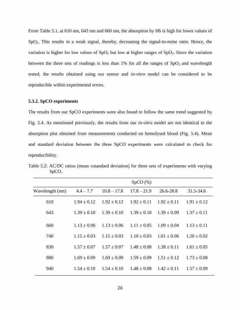
5.3.2. SpCO experiments
The results from our SpCO experiments were also found to follow the same trend suggested by
Fig. 5.4. As mentioned previously, the results from our in-vitro model are not identical to the
absorption plot obtained from measurements conducted on hemolysed blood (Fig. 5.4). Mean
and standard deviation between the three SpCO experiments were calculated to check for
reproducibility.
Table 5.2: AC/DC ratios (mean ±standard deviation) for three sets of experiments with varying
SpCO.
SpCO (%)
Wavelength (nm) 4.4 – 7.7 10.8 – 17.8 17.8 – 21.9
26.6-28.8
31.5-34.6
610 1.94 ± 0.12
1.92 ± 0.12 1.92 ± 0.11 1.92 ± 0.11 1.91 ± 0.12
643 1.39 ± 0.10
1.39 ± 0.10 1.39 ± 0.10 1.39 ± 0.09 1.37 ± 0.11
660 1.13 ± 0.06 1.13 ± 0.06 1.11 ± 0.05 1.09 ± 0.04 1.13 ± 0.11
740 1.15 ± 0.03
1.15 ± 0.03 1.10 ± 0.03 1.01 ± 0.06 1.20 ± 0.02
830 1.57 ± 0.07 1.57 ± 0.07 1.48 ± 0.08 1.38 ± 0.11 1.61 ± 0.05
880 1.69 ± 0.09 1.69 ± 0.09 1.59 ± 0.09 1.51 ± 0.12 1.73 ± 0.08
940 1.54 ± 0.10 1.54 ± 0.10 1.48 ± 0.08 1.42 ± 0.11 1.57 ± 0.09
27
Table 5.2 shows that the standard deviation between the absorption values for three sets of
experiments is low at all wavelengths and concentration ranges considered. At 610nm, the
absorption by HbCO is high. This results in a weak signal that decreases the signal-to-noise ratio.
Hence, the variation is relatively higher for all ranges of SpCO at this wavelength. The standard
deviation between the readings is less than 1% for all wavelengths at all ranges of SpCO. Hence,
these results can be considered to be reproducible within experimental errors.
5.3.3. Assessing the validity of the tissue simulator
As mentioned in Section 5.1.3, experiments were conducted using the commercial Masimo pulse
oximeter on our in-vitro simulator with simultaneous blood sampling using IL 682 CO-
Oximeter. Standard deviation was calculated between IL 682 data and the data from the Masimo
pulse oximeter obtained from our in-vitro model. The mean standard deviation between the two
data sets was found to be ±2.9% for SpO2 between 50-100%. This error is acceptable because
commercially available pulse oximeters are calibrated on humans and not on in-vitro models.
Thus, the model can be used for the HbCO determination.
Hence from these preliminary experiments, it is shown that the results obtained from our
model and our sensor can be used for measurement of both SpO2 and SpCO.
28
Chapter 6: Theoretical modeling for simultaneous measurement of SpO2 and SpCO
6.1. Need for a theoretical model
The wavelengths required for accurate monitoring of SpO2 can be identified based on Fig. 2.2.
Assuming, HbCO is absent, SpO2 measurement involves two unknowns, the concentration of
HbO2 and Hb. To calculate these two unknowns, we would need a minimum of two wavelengths.
One wavelength can be chosen from the region of maximum sensitivity to changes in SpO2 and
the other wavelength can be chosen from an isobestic wavelength region. The ratio of absorption
at those two wavelengths can be used to calculate SpO2. However, to determine the effect
different factors would have on SpO2 measurements, like temperature induced changes in LED
peak wavelengths, time consuming and expensive experiments have to be conducted.
Alternatively, the sensitivity at different wavelengths can be found using a theoretical model.
The need for a theoretical model is more pronounced in the case of SpCO measurement because,
in the presence of HbCO, there are three unknown variables (concentrations of HbO2, Hb and
HbCO) involved in SpO2 and SpCO measurement. A minimum of three wavelengths are
required to calculate these variables simultaneously. Identifying experimentally three
wavelengths that would have good sensitivity to changes in both SpO2 and SpCO solely based on
Fig. 2.2 will be time consuming and expensive. Hence, a theoretical model becomes a practical
and effective means to identify the wavelengths for simultaneous measurement of SpO2 and
SpCO.
The laws that can be used to obtain a theoretical model should simulate the effects of light
interaction with lood and tissue. Twerky’s multiple scattering theory has so far een the most
successful for modeling whole blood for in-vitro oximetry [26-27]. Similarly, a model based on
3-D photon diffusion theory has been used to effectively simulate light propagation through
29
biological tissues [27-28]. However, the mathematical models that are based on these theories
are more complex. In spite of using these complex theories to model light interaction with blood
and tissue, a pulse oximeter must be finally calibrated on humans. This is because there is no
standard to validate the results that will be obtained from these models [29]. Although Beer-
Lamberts law is not applicable to pulse oximetry, the final empirical calibration performed on
the device based on in-vivo measurements compensates for the simplifications made in the
theoretical model [30]. Therefore, Beer-Lamberts law was used to develop a theoretical
formulation to facilitate the development of a simple algorithm for simultaneous measurement of
SpO2 and SpCO.
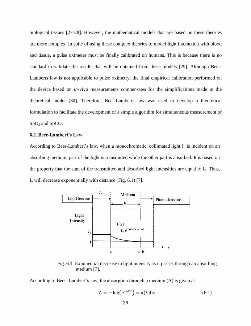
6.2. Beer-Lambert’s Law
According to Beer-Lam ert’s law, when a monochromatic, collimated light Io is incident on an
absorbing medium, part of the light is transmitted while the other part is absorbed. It is based on
the property that the sum of the transmitted and absorbed light intensities are equal to Io. Thus,
Io will decrease exponentially with distance (Fig. 6.1) [7].
Fig. 6.1. Exponential decrease in light intensity as it passes through an absorbing
medium [7].
According to Beer- Lam ert’s law, the a sorption through a medium (A) is given as
( ) ( ) (6.1)
30
where, ( ) is the absorptivity for a given wavelength
b is the path length
c is the concentration of the absorbing substance
If there are multiple absorbers in the medium, each absorbing substance contributes to the total
absorbance corresponding to its concentration and absorptivity. Thus, the total absorbance for n
absorbing substance is
( ) ( ) ( ) ( ) ∑ ( ) (6.2)
where, i ( ) represent the absorptivity, bi represent the path length and ci is the concentration of
the absorbing substance i, respectively.
Strictly, Beer-Lam ert’s law does not account for light scattering or specular light reflection
at the surface of a biological medium. In reflectance pulse oximetry, as in the case of
transmission mode, the principle quantity measured is the change in light absorption. The
theoretical model developed based on Beer-Lam ert’s law was used to estimate the relative
change in the absorption ratio corresponding to the change in SpO2 or SpCO. By quantifying this
relative change in ratio, the sensitivity of different wavelengths to changes in SpO2 or SpCO can
be identified. To avoid inaccuracies associated with any attempt to utilize a theoretical
formulation to describe light propagation through biological tissues and obtain a quantitatively
accurate algorithm to determine SpO2 or SpCO, commercial pulse oximeters rely on empirical
calibration [15].
A study evaluating the relationship between SaO2 and the R/IR ac-dc ratio, used in pulse
oximeters under a variety of physiological conditions, like different blood volumes, hematocrit,
pigmentation and finger thickness, show that in pulse oximeters using fixed calibration curves
31
based on empirical measurements, errors introduced by interfering variables should be less than a
few percent in the clinically significant range of 70-100% [28]. Hence empirical calibration of
the device has been successfully employed for SpO2 measurement in commercially available
pulse oximeters. Similarly such calibration can be employed for simultaneous measurement of
SpO2 and SpCO.
6.3. Derivation of the theoretical model
As mentioned in Chapter 2, at wavelengths used in pulse oximetry, Hb and its derivatives are
the main absorbers of light in blood. The most dominant Hb derivatives are HbO2, Hb, HbCO
and MetHb. The measurement of SpO2 by a pulse oximeter is based on the assumption that the
concentration of HbCO or MetHb in blood is negligible. For the purpose of this thesis, we will
assume that the concentration of MetHb is negligible. The blood that was used in our
experiments had negligible concentrations of MetHb. Hence, concentrations of HbO2, HbCO
and Hb are the three unknowns that need to be calculated and hence a minimum of three
wavelengths were required to calculate these unknowns.
Literature search on simultaneous measurement of SpCO and SpO2 yielded only two results.
Lee et al. [31] developed two theoretical models, one based on Beer-Lam ert’s law and the other
based on photon diffusion theory. Using the theoretical model based on Beer-Lam ert’s law, the
sensitivity of different combinations of three wavelengths to changes in SpCO and SpO2 were
determined. The wavelengths used by Lee were reported to be between 600-940 nm. Then,
using an in-vitro model which mimics the absorption properties of the tissue, absorption values
were obtained from blood samples with a known concentration of HbCO and HbO2 at these
wavelength combinations and the sensitivity of the wavelength ratios to changes in SpO2 and
SpCO were verified experimentally. The paper reports good accuracy for simultaneous in-vitro
32
measurement of SpCO and SpO2 at 630 nm, 660 nm and 950 nm, but it does not discuss the
sensitivity of other wavelength combinations to changes in SpCO and SpO2. Pieralli et al. [32]
developed a theoretical model for SpO2 and SpCO measurement also based on Beer-Lam ert’s
law. Three laser diodes (660 nm, 830 nm and 1060 nm) were used in a prototype sensor. The
paper discusses the results of a series of in-vivo SpO2 and SpCO experiments where SpCO was
varied from 3.5%-8%. Discrepancies were reported in 3 out of 440 human tests. Since there are
no LED’s availa le at 1060 nm, the use of laser diodes makes the hardware more complicated,
bulky and expensive. Hence, the use of this specific wavelength is not practical in a pulse
oximeter sensor. Although both papers do not discuss the sensitivity of other wavelength
combinations to changes in SpCO and SpO2, they suggest that the use of a three wavelength
combination is sufficient for simultaneous measurements of SpCO and SpO2 using pulse
oximeters. Despite these developments in identifying potential wavelengths, a pulse oximeter
that would simultaneously measure SpO2 and SpCO was not commercially available until
Masimo Rad-57 was commercialized. As mentioned previously, a minimum of three
wavelengths are required to measure SpO2 and SpCO simultaneously. Based on this assumption,
a theoretical model was be established by applying Beer-Lam ert’s law.
According to Beer-Lam ert’s law, the total a sor ance for n a sor ing su stances is the sum
of absorbance of each substance corresponding to its concentration, absorptivity and path length.
For simultaneous measurement of SpCO and SpO2, the total absorbance for three homogenously
mixed absorbing substances (HbO2, RHb and HbCO) at each wavelength is given as
( ) ( ) ( ) ( ) (6.3)
( ) ( ) ( ) ( ) (6.4)
( ) ( ) ( ) ( ) (6.5)
33
where,
a11, a21, a31 are the absorptivities of HbO2, H and H CO at wavelength 1, respectively,
a12, a22, a32 are the absorptivities of HbO2, H and H CO at wavelength 2, respectively,
a13, a23, a33 are the absorptivities of HbO2, H and H CO at wavelength 3, respectively,
1, 2, 3 are the chosen wavelengths,
b is the optical path length.
Dividing equations (Eq. 6.3), (Eq. 6.4), (Eq. 6.5) by HbO2, we get
( )
( ) ( ) (6.6)
( )
( ) ( ) (6.7)
( )
( ) ( ) (6.8)
where,
c2= Hb/HbO2
c1= HbCO/HbO2
Let r1 = ( )
( )
[ ( ) ( )]
[ ( ) ( )] (6.9)
and r2 = ( )
( )
[ ( ) ( )]
[ ( ) ( )] (6.10)
From Eq. 6.9 and Eq. 6.10, we get
r1 [ ( ) ( )] = ( ) ( ) (6.11)
r2 [ ( ) ( )] = ( ) ( ) (6.12)
34
Grouping the c1 and c2 terms in Eq. 6.11 and Eq. 6.12,
( ) ( ) ( ) (6.13)
( ) ( ) ( ) (6.14)
Simultaneous equations (Eq. 6.13- Eq. 6.14) can be solved for c1 and c2 using Cramer’s rule as
shown below.
△ [( ) ( )( ) ( )
] (6.15)
[( ) ( )( ) ( )
] (6.16)
[ ( ) ( ) ( ) ( )
] (6.17)
Solving for △ using Eq. 6.15,
△ ( )( ) ( )( )
=
Simplification yields,
△= ( ) ( ) ( ) ( )
= ( ) ( ) ( ) (6.18)
Solving for using Eq. 6.16,
[( ) ( ) ( )( )]
35
=
[ ]
Simplification yields,
=
[ ( ) ( ) ( ) (
)]
=
[
( ) ( ) (
)] (6.19)
Solving for using Eq. 6.17,
[ ( )( ) ( )( )]
=
[ ]
Simplification yields,
=
[ ( ) ( ) ( ) ( )]
=
[ ( ) ( ) ( )] (6.20)
The formula for SpO2 and SpCO is given by Eq. 6.21 and Eq. 6.22.
SpO2 = [ ]
[ ] [ ] [ ]
(6.21)
[ ]
[ ] [ ] [ ]
(6.22)
Substituting the values of △, c1 and c2 in Eq. 6.21,
[ ( ) ( ) ( )]
=
=
[ ( ) ( ) ( )]
36
=
[ ( ) ( ) ( )] =
[ ( ) ( ) ( )]
=
( ) ( ) ( )
( ) ( )
( ) ( ) ( )
( (6.23)
Eq. 6.23 can be written as
SpO2 =
(6.24)
where,
A=( )
B=( )
C=( )
D=( )
E=( )
F=( )
Similarly, substituting for c1, c2 and △, in Eq. 6.22,
SpCO=
[ ( a ) ( ) ( )]
( a a ) ( )
= [ ( a ) ( ) ( )]
( (6.25)
37
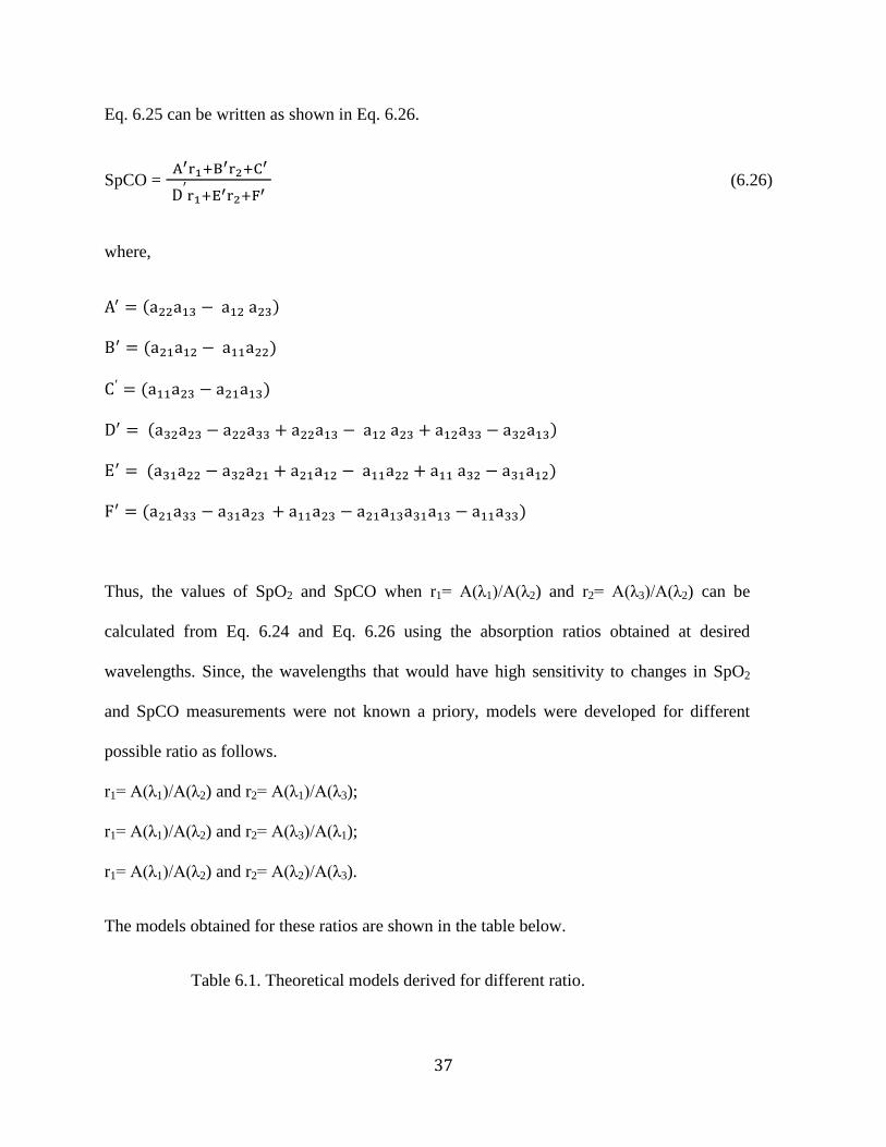
Eq. 6.25 can be written as shown in Eq. 6.26.
SpCO =
(6.26)
where,
( )
( )
( )
( )
( )
( )
Thus, the values of SpO2 and SpCO when r1= A( 1)/A( 2) and r2= A( 3)/A( 2) can be
calculated from Eq. 6.24 and Eq. 6.26 using the absorption ratios obtained at desired
wavelengths. Since, the wavelengths that would have high sensitivity to changes in SpO2
and SpCO measurements were not known a priory, models were developed for different
possible ratio as follows.
r1= A( 1)/A( 2) and r2= A( 1)/A( 3);
r1= A( 1)/A( 2) and r2= A( 3)/A( 1);
r1= A( 1)/A( 2) and r2= A( 2)/A( 3).
The models obtained for these ratios are shown in the table below.
Table 6.1. Theoretical models derived for different ratio.

38
r1= A(λ1)/A(λ2) and r2= A(λ1)/A(λ3)
SpO2=
( ) ( ) ( )
( ) ( )
( ) ( ) ( )
( )
SpCO=
( ) ( ) ( )
( ) ( )
=
( ) ( ) ( )
( )
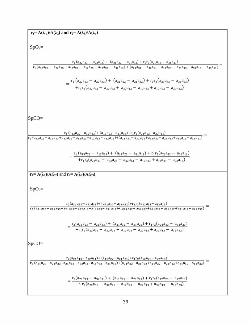
39
r1= A(λ 1)/A(λ2) and r2= A(λ3)/A(λ1)
SpO2=
( ) ( ) ( )
( ) ( )
( ) ( ) ( )
( )
SpCO=
( ) ( ) ( )
( ) ( )
( ) ( ) ( )
( )
r1= A(λ1)/A(λ2) and r2= A(λ2)/A(λ3)
SpO2=
( ) ( ) ( )
( ) ( )
( ) ( ) ( )
( )
SpCO=
( ) ( ) ( )
( ) ( )
( ) ( ) ( )
( )
40
Using these theoretical simulations, wavelength combinations that have high sensitivity to
changes in both SpO2 and SpCO can be obtained. Using the wavelengths identified by the
theoretical simulation described above, an algorithm that enables simultaneous measurement of
SpO2 and SpCO can be obtained. Note that a noninvasive device which can measure SpCO alone
can be developed. However, at any given point, the derivatives of Hb are in chemical equilibrium
with each other. Hence, as the concentrations of HbCO decreases, the relative concentration of
HbO2 increases and vice versa. Therefore, we need a minimum of three wavelengths to measure
the concentrations of Hb, HbO2 and HbCO in order to calculate SpCO. As shown in Eq. 6.21-
6.22, using these concentrations of Hb, HbO2 and HbCO necessary to calculate SpCO, SpO2 can
also be calculated. This makes simultaneous measurement of SpCO and SpO2 more
advantageous commercially because it enables measurement of additional physiological variable
using these same concentration values.
6.4. Wavelength ratio selection
As mentioned previously, in the presence of HbCO, a minimum of three wavelengths are
required for simultaneous measurement of SpO2 and SpCO. As shown in Fig. 2.1, the absorption
in the wavelength regions between 600 nm and 660 nm increases with increase in SpCO.
Between 800 nm to 950 nm, the change in absorption due to changes in SpCO is opposite to the
effect observed in the 600-660 nm region. Hence, a ratio of two wavelengths, one from the 600-
660 nm region and another from 900-940 nm region will have relatively high sensitivity to
changes in SpCO. Two wavelengths (660 nm and 940 nm) that have the highest sensitivity to
changes in SpO2 can be used for simultaneous measurements of SpO2 and SpCO. Apart from
A660/A940, a second ratio of any wavelengths between 600 - 660 nm as well as 940 nm, will have
good sensitivity to changes in SpCO. In the sensor used in our lab, there are two LEDs available
41
in this wavelength region, 610 nm and 643 nm. Therefore, r1 will correspond to A660/A940 and r2
can be A643/A940 or A610/A940. These ratios of r1 and r2 will have high sensitivity to changes in
SpCO and can be used for simultaneous measurement of SpCO and SpO2. Although both ratios
of A643/A940 and A610/A940 will have relatively high sensitivity to changes in SpO2, A643/A940 will
have a higher sensitivity than A610/A940 (Fig. 2.1). Also, the absorption by blood is high around
600 nm and that can cause a low signal to noise ratio at 610 nm. Hence, r1 = A660/A940 and r2 =
A643/A940 will have high sensitivity to both SpO2 and SpCO and can be used for simultaneous
measurement of SpO2 and SpCO. Theoretical simulations were conducted using these
wavelengths to confirm the above conclusions.
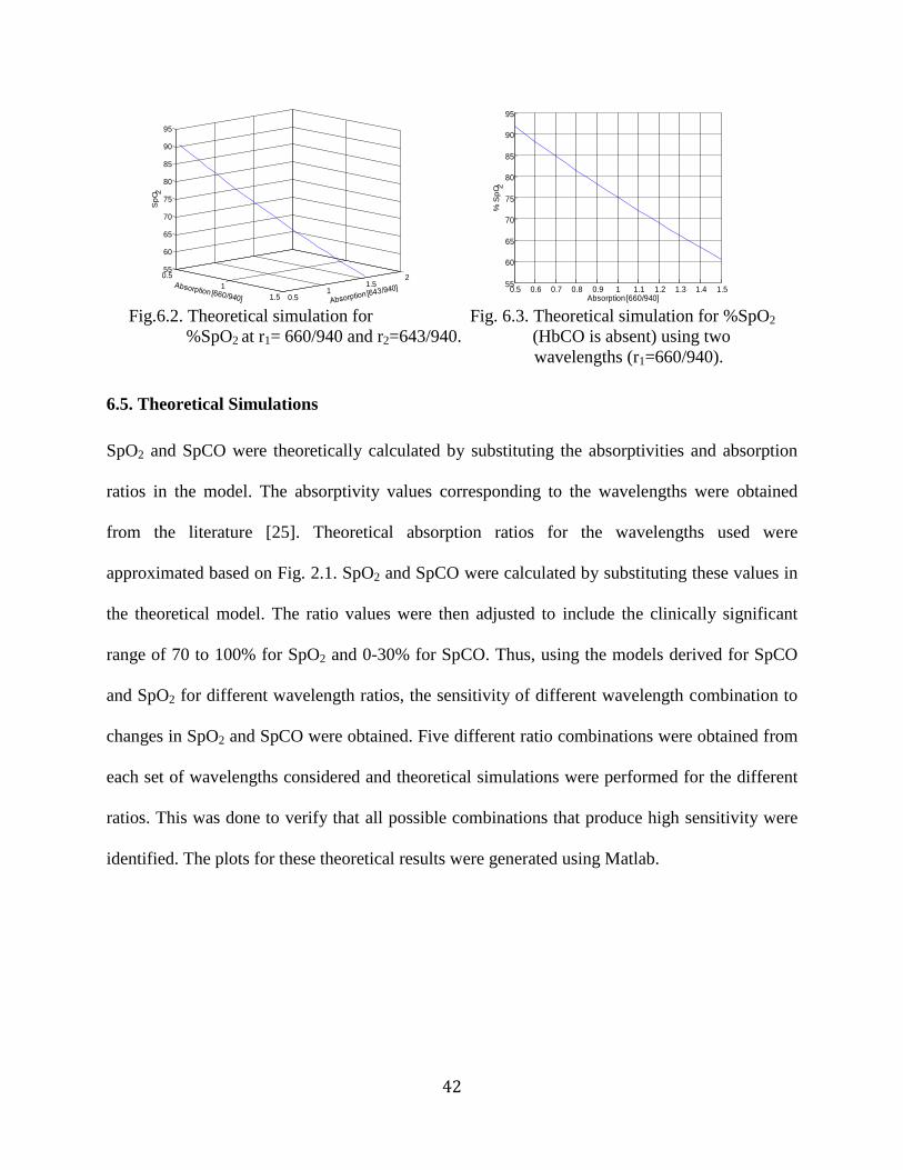
6.4.1. Validation of the theoretical model for r1= A (660/940) and r2= A (643/940)
In order to validate the theroretical model, theoretical simulation for SpO2 in the absence of
HbCO was obtained at r1=660/940 and r2=643/940, by substituting HbCO=0 in Eq. 6.21. When
HbCO is absent, SpO2 value computed by the three-wavelength model and the two-wavelength
model (used in commercially available pulse oximeters to measure SpO2 in the absence of
HbCO) should be approximately the same. Hence, SpO2 calculated from the three wavelength
model using r1= A(660)/(940) and r2= A(643)/(940) was compared to the results obtained for r1=
A(660)/(940). It was found that SpO2 calculated from the two and three wavelength model were
approximately the same when HbCO=0 (Fig. 6.2-6.3). Therefore, these theoretical simulations,
verified that the sensitivity of 660/940 and 643/940 to changes in SpO2 in the absence of HbCO
is approximately the same as the sensitivity of 660/940. Hence, the theoretical model was
validated for use of 660 nm, 643 nm and 940 nm as the primary wavelengths.
42
Fig.6.2. Theoretical simulation for Fig. 6.3. Theoretical simulation for %SpO2
%SpO2 at r1= 660/940 and r2=643/940. (HbCO is absent) using two
wavelengths (r1=660/940).
6.5. Theoretical Simulations
SpO2 and SpCO were theoretically calculated by substituting the absorptivities and absorption
ratios in the model. The absorptivity values corresponding to the wavelengths were obtained
from the literature [25]. Theoretical absorption ratios for the wavelengths used were
approximated based on Fig. 2.1. SpO2 and SpCO were calculated by substituting these values in
the theoretical model. The ratio values were then adjusted to include the clinically significant
range of 70 to 100% for SpO2 and 0-30% for SpCO. Thus, using the models derived for SpCO
and SpO2 for different wavelength ratios, the sensitivity of different wavelength combination to
changes in SpO2 and SpCO were obtained. Five different ratio combinations were obtained from
each set of wavelengths considered and theoretical simulations were performed for the different
ratios. This was done to verify that all possible combinations that produce high sensitivity were
identified. The plots for these theoretical results were generated using Matlab.
0.5
1
1.5 0.51
1.52
55
60
65
70
75
80
85
90
95
Sp
O 2
0.5 0.6 0.7 0.8 0.9 1 1.1 1.2 1.3 1.4 1.555
60
65
70
75
80
85
90
95
Absorption [660/940]
% S
pO 2
43
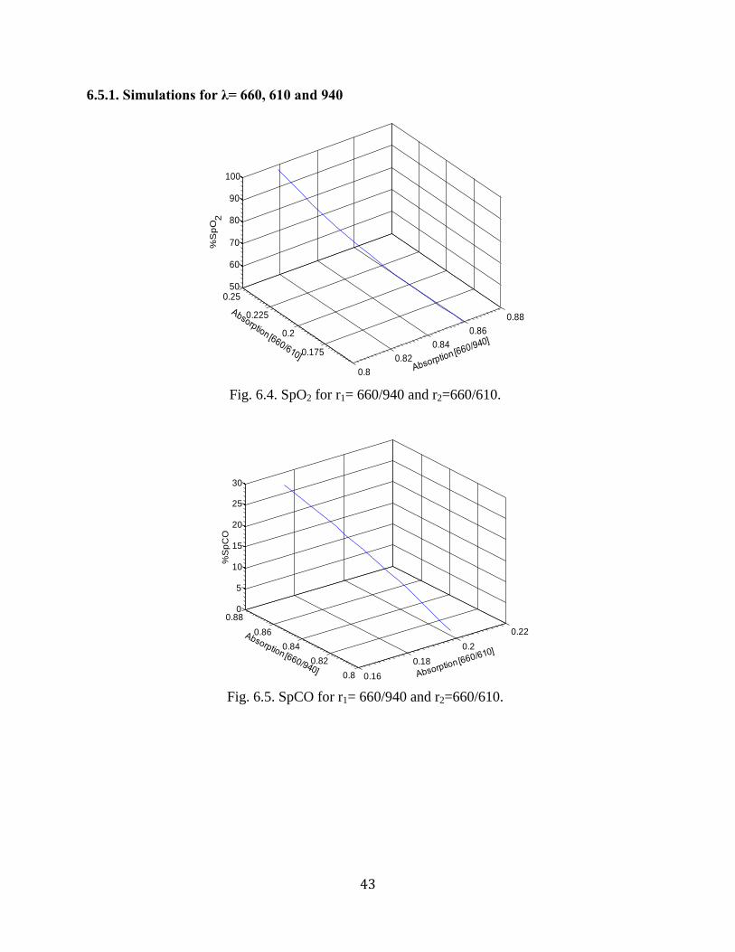
6.5.1. Simulations for λ= 660, 610 and 940
Fig. 6.4. SpO2 for r1= 660/940 and r2=660/610.
Fig. 6.5. SpCO for r1= 660/940 and r2=660/610.
0.8
0.82
0.84
0.86
0.88
0.175
0.2
0.225
0.2550
60
70
80
90
100
%S
pO
2
0.16
0.18
0.2
0.22
0.8
0.82
0.84
0.86
0.880
5
10
15
20
25
30
%S
pC
O
44
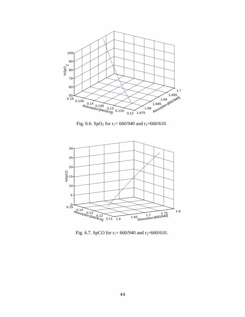
Fig. 6.6. SpO2 for r1= 660/940 and r2=660/610.
Fig. 6.7. SpCO for r1= 660/940 and r2=660/610.
1.675
1.68
1.685
1.69
1.695
1.7
0.120.125
0.130.135
0.140.145
0.1550
60
70
80
90
100
%S
pO
2
1.61.65
1.71.75
1.8
0.110.12
0.130.14
0.150
5
10
15
20
25
30
%S
pC
O
45
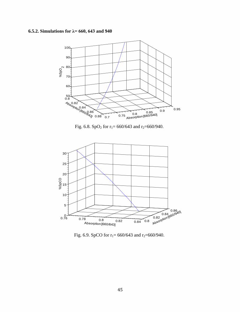
6.5.2. Simulations for λ= 660, 643 and 940
Fig. 6.8. SpO2 for r1= 660/643 and r2=660/940.
Fig. 6.9. SpCO for r1= 660/643 and r2=660/940.
0.8
0.82
0.84
0.86
0.88 0.70.75
0.80.85
0.90.95
50
60
70
80
90
100
%S
pO
2
0.76 0.78 0.8 0.82 0.84 0.80.82
0.840.86
0
5
10
15
20
25
30
%S
pC
O
46
Fig. 6.10. SpO2 for r1= 660/940 and r2=643/940.
Fig. 6.11. SpCO for r1= 660/940 and r2=643/940.
0.40.60.811.21.4
0.5
1
1.5
50
60
70
80
90
100
%S
pO
2
0.50.60.70.80.9
0.5
1
1.5
0
5
10
15
20
25
30
%S
pC
O
47
Fig. 6.12. SpO2 for r1= 660/940 and r2=940/643.
Fig. 6.13. SpCO for r1= 660/940 and r2=940/643.
0.50.55
0.60.65
0.70.75
0.8
0.82
0.84
0.86
0.8850
60
70
80
90
100
%S
pO
2
0.64
0.66
0.68
0.7
0.72 0.820.83
0.840.85
0.86
0
5
10
15
20
25
30
%S
pC
O
48
Fig. 6.14. SpO2 for r1= 940/643and r2=940/660.
Fig. 6.15. SpCO for r1= 940/643and r2=940/660.
0.880.9
0.920.94
0.960.98
1
0.65
0.7
0.75
0.8
0.85
0.950
60
70
80
90
100
%S
pO
2
0.70.72
0.740.76
0.780.8
0.9 0.91 0.92 0.93 0.94 0.95 0.96
0
5
10
15
20
25
30
%S
pC
O
49
Fig. 6.16. SpO2 for r1= 940/660and r2=643/940.
Fig. 6.17. SpCO for r1= 940/660and r2=643/940.
1.31.4
1.51.6
1.71.8 0.86
0.88
0.9
0.9250
60
70
80
90
100
%S
pO
2
1.351.4
1.451.5
1.551.6
0.84
0.845
0.85
0.855
0.86
0.8650
5
10
15
20
25
30
%S
pC
O
50
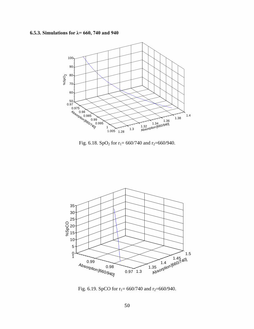
6.5.3. Simulations for λ= 660, 740 and 940
Fig. 6.18. SpO2 for r1= 660/740 and r2=660/940.
Fig. 6.19. SpCO for r1= 660/740 and r2=660/940.
0.97
0.9750.98
0.985
0.990.995
1
1.005 1.281.3
1.321.34
1.361.38
1.4
50
60
70
80
90
100
%S
pO
2
1.31.35
1.41.45
1.5
0.97
0.98
0.99
10
5
10
15
20
25
30
35
%S
pC
O
51
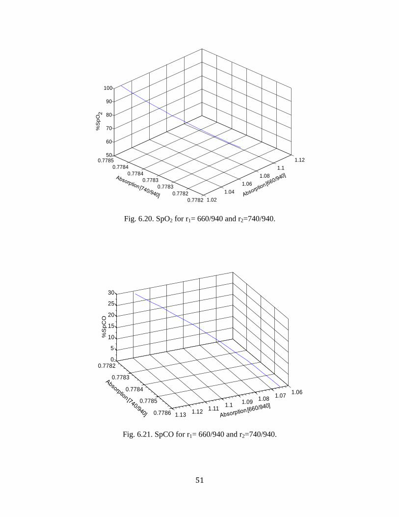
Fig. 6.20. SpO2 for r1= 660/940 and r2=740/940.
Fig. 6.21. SpCO for r1= 660/940 and r2=740/940.
1.02
1.04
1.06
1.08
1.1
1.12
0.7782
0.7782
0.7783
0.7783
0.7784
0.7784
0.778550
60
70
80
90
100
%S
pO
2
1.061.07
1.081.09
1.11.11
1.121.13
0.7782
0.7783
0.7784
0.7785
0.7786
0
5
10
15
20
25
30
%S
pC
O
52
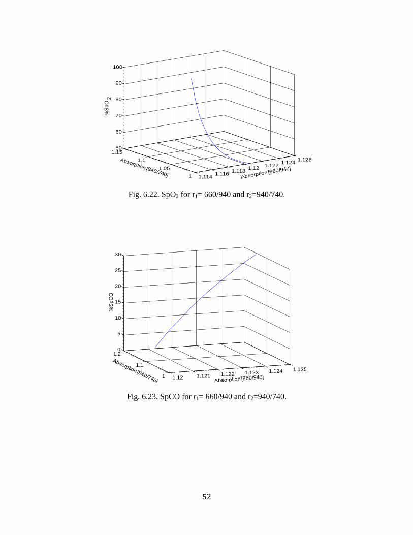
Fig. 6.22. SpO2 for r1= 660/940 and r2=940/740.
Fig. 6.23. SpCO for r1= 660/940 and r2=940/740.
1.1141.116
1.1181.12
1.1221.124
1.126
1
1.05
1.1
1.1550
60
70
80
90
100
%S
pO
2
1.12 1.121 1.122 1.123 1.124 1.125
1
1.1
1.20
5
10
15
20
25
30
%S
pC
O
53
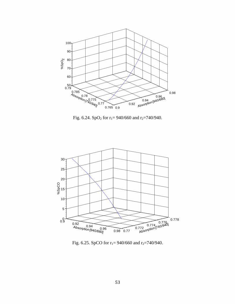
Fig. 6.24. SpO2 for r1= 940/660 and r2=740/940.
Fig. 6.25. SpCO for r1= 940/660 and r2=740/940.
0.9
0.920.94
0.960.98
0.765
0.77
0.775
0.78
0.785
0.7950
60
70
80
90
100
%S
pO
2
0.90.92
0.940.96
0.98 0.770.772
0.7740.776
0.7780
5
10
15
20
25
30
%S
pC
O
54
Fig. 6.26. SpO2 for r1= 940/660 and r2=940/740.
Fig. 6.27. SpCO for r1= 940/660 and r2=940/740.
1.26
1.28
1.3
1.32
1.34 0.942
0.944
0.946
0.948
0.95
0.952
0.954
50
60
70
80
90
100
%S
pO
2
0.9450.95
0.9550.96 1.25
1.3
1.35
1.4
0
5
10
15
20
25
30
35
%S
pC
O
55
6.5.4. Simulations for λ= 660, 830 and 940
Fig. 6.28. SpO2 for r1= 660/940 and r2=660/830.
Fig. 6.29. SpCO for r1= 660/940 and r2=660/830.
0.90.91
0.92
0.930.94
0.76
0.78
0.8
0.82
0.84
60
80
100%
Sp
O2
0.77
0.78
0.79
0.8
0.81
0.905
0.91
0.915
0.92
0.9250
10
20
30
%S
pC
O
56
Fig. 6.30. SpO2 for r1= 660/940 and r2=830/940.
Fig. 6.31. SpCO for r1= 660/940 and r2=830/940.
1.41.45
1.51.55
1.6
0.880.89
0.90.91
0.9250
60
70
80
90
100
%S
pO
2
1.441
1.442
1.443
1.444
0.890.895
0.90.905
0.91
0
5
10
15
20
25
30
%S
pC
O
57
Fig. 6.32. SpO2 for r1= 660/940 and r2=940/830.
Fig. 6.32. SpCO for r1= 660/940 and r2=940/830.
1.0741.075
1.0761.077
1.0781.079 1.04
1.06
1.08
1.150
60
70
80
90
100%
Sp
O 2
1.0765
1.077
1.0775
1.078
1.0785
1.079 1.051.055
1.061.065
1.071.075
0
5
10
15
20
25
30
%S
pC
O
58
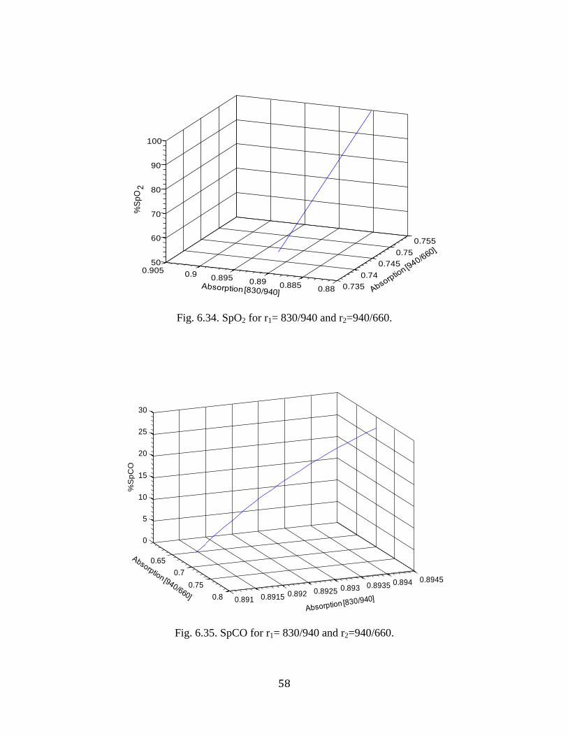
Fig. 6.34. SpO2 for r1= 830/940 and r2=940/660.
Fig. 6.35. SpCO for r1= 830/940 and r2=940/660.
0.735
0.74
0.745
0.75
0.755
0.880.885
0.890.895
0.90.905
50
60
70
80
90
100%
Sp
O2
0.65
0.7
0.75
0.8 0.891 0.8915 0.892 0.8925 0.893 0.8935 0.894 0.8945
0
5
10
15
20
25
30
%S
pC
O
59
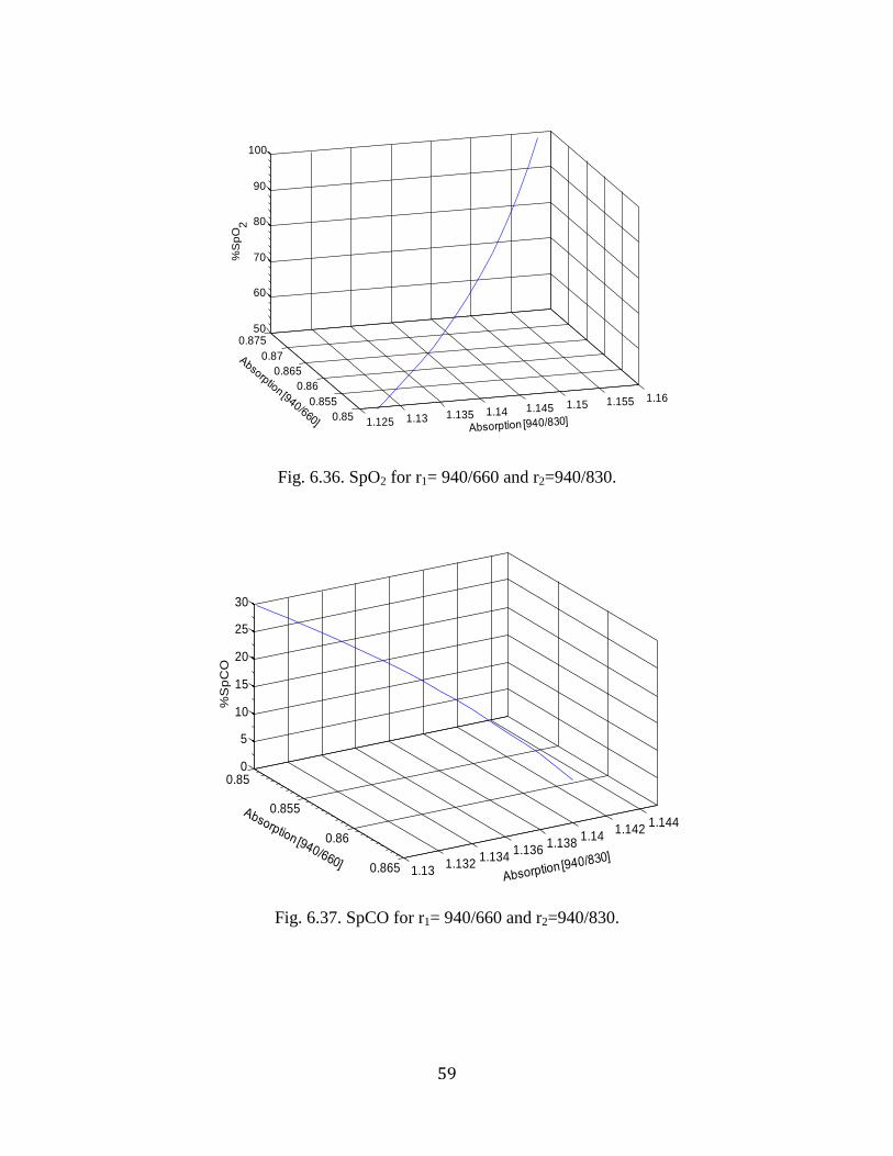
Fig. 6.36. SpO2 for r1= 940/660 and r2=940/830.
Fig. 6.37. SpCO for r1= 940/660 and r2=940/830.
1.125 1.13 1.135 1.14 1.145 1.15 1.155 1.16
0.85
0.855
0.86
0.865
0.87
0.87550
60
70
80
90
100
%S
pO
2
0.85
0.855
0.86
0.865 1.131.132
1.1341.136
1.1381.14
1.1421.144
0
5
10
15
20
25
30
%S
pC
O
60
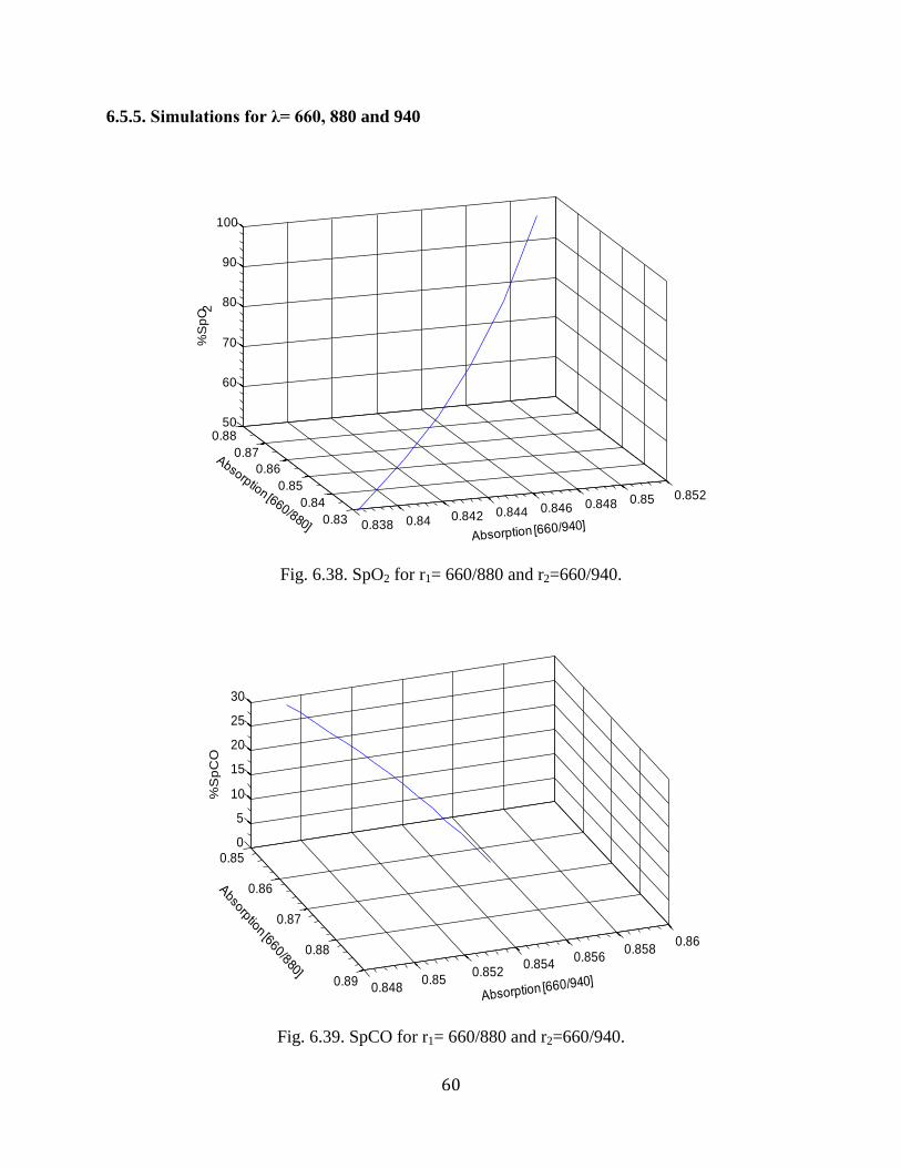
6.5.5. Simulations for λ= 660, 880 and 940
Fig. 6.38. SpO2 for r1= 660/880 and r2=660/940.
Fig. 6.39. SpCO for r1= 660/880 and r2=660/940.
0.838 0.84 0.842 0.844 0.846 0.848 0.85 0.852
0.83
0.84
0.85
0.86
0.87
0.8850
60
70
80
90
100
%S
pO2
0.85
0.86
0.87
0.88
0.890.848
0.850.852
0.8540.856
0.8580.86
0
5
10
15
20
25
30
%S
pC
O
61
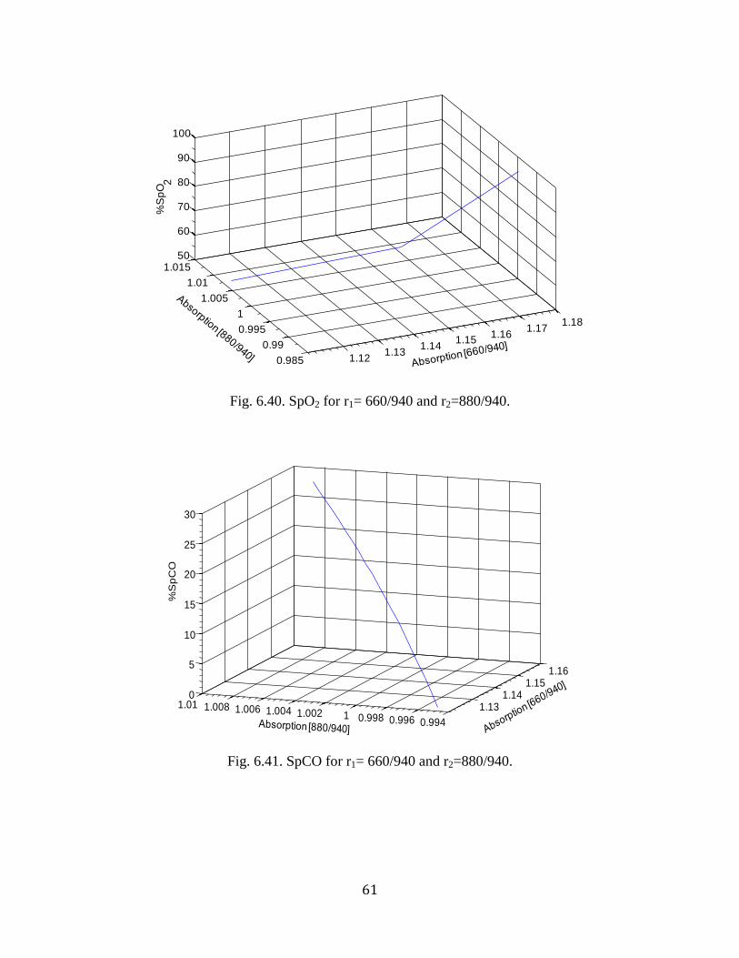
Fig. 6.40. SpO2 for r1= 660/940 and r2=880/940.
Fig. 6.41. SpCO for r1= 660/940 and r2=880/940.
1.121.13
1.141.15
1.161.17
1.18
0.985
0.99
0.995
1
1.005
1.01
1.01550
60
70
80
90
100
%S
pO
2
1.131.14
1.151.16
0.9940.9960.99811.0021.0041.0061.0081.010
5
10
15
20
25
30
%S
pC
O
62
Fig. 6.42. SpO2 for r1= 660/940 and r2=940/880.
Fig. 6.43. SpCO for r1= 660/940 and r2=940/880.
1.5
1.55
1.6
0.9
0.92
0.94
0.9650
60
70
80
90
100
%S
pO
2
1.51.52
1.541.56
1.581.6 0.91
0.92
0.93
0.94
0.95
0
5
10
15
20
25
30
%S
pC
O
63
Fig. 6.44. SpO2 for r1= 940/660 and r2=880/940.
Fig. 6.45. SpCO for r1= 940/660 and r2=880/940.
0.656
0.658
0.66
0.662
0.9951
1.0051.01
1.015
50
60
70
80
90
100
%S
pO
2
0.65750.658
0.65850.659
0.65950.66
0.66050.661
1.01
1.015
1.02
1.025
1.030
5
10
15
20
25
30
%S
pC
O
64
Fig. 6.46. SpO2 for r1= 940/660 and r2=940/880.
Fig. 6.47. SpCO for r1= 940/660 and r2=940/880.
0.990.995
11.005
1.011.015
1.021.025
0.95
1
1.05
1.150
60
70
80
90
100
%S
pO
2
0.990.99511.0051.011.015
0.995
1
1.005
1.01
1.015
0
5
10
15
20
25
30
%S
pC
O
65
6.6. Discussion
Practically, a small change in the value of SpCO will cause a large change in the absorption
value if the wavelength is sensitive to changes in SpCO. Theoretical simulations confirmed that
the absorption ratios at 660/940 and 643/940 had the highest sensitivity to changes in SpCO (Fig.
6.10-6.11). Based on the theoretical results shown previously, Table 6.2 was compiled to
compare the sensitivities for different wavelength combinations. The table summerizes the
differences in the ratio r1 and r2 corresponding to a 50% decrease in SpO2 and an increase in
SpCO from 0-30% are calculated. NA in the table indicates those wavelength ratios at which
SpO2 and SpCO could not be obtained within the clinically significant range.
From Table 6.2, it was concluded that the absorption at 643/940 and 660/940 had the highest
relative change in absorption corresponding to changes in SpO2 and SpCO. Therefore, the
wavelength ratios 660/940 and 643/940 have relatively high sensitivity to changes in SpO2 and
SpCO as concluded from preliminary experiments.
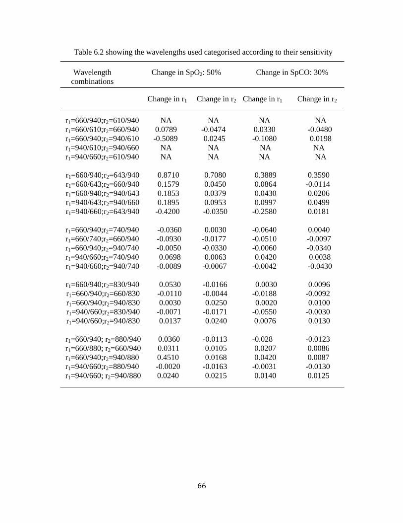
66
Table 6.2 showing the wavelengths used categorised according to their sensitivity
Wavelength
combinations
Change in SpO2: 50% Change in SpCO: 30%
Change in r1 Change in r2 Change in r1 Change in r2
r1=660/940;r2=610/940
r1=660/610;r2=660/940
r1=660/940;r2=940/610
r1=940/610;r2=940/660
r1=940/660;r2=610/940
NA
0.0789
-0.5089
NA
NA
NA
-0.0474
0.0245
NA
NA
NA
0.0330
-0.1080
NA
NA
NA
-0.0480
0.0198
NA
NA
r1=660/940;r2=643/940
r1=660/643;r2=660/940
r1=660/940;r2=940/643
r1=940/643;r2=940/660
r1=940/660;r2=643/940
0.8710
0.1579
0.1853
0.1895
-0.4200
0.7080
0.0450
0.0379
0.0953
-0.0350
0.3889
0.0864
0.0430
0.0997
-0.2580
0.3590
-0.0114
0.0206
0.0499
0.0181
r1=660/940;r2=740/940
r1=660/740;r2=660/940
r1=660/940;r2=940/740
r1=940/660;r2=740/940
r1=940/660;r2=940/740
-0.0360
-0.0930
-0.0050
0.0698
-0.0089
0.0030
-0.0177
-0.0330
0.0063
-0.0067
-0.0640
-0.0510
-0.0060
0.0420
-0.0042
0.0040
-0.0097
-0.0340
0.0038
-0.0430
r1=660/940;r2=830/940
r1=660/940;r2=660/830
r1=660/940;r2=940/830
r1=940/660;r2=830/940
r1=940/660;r2=940/830
0.0530
-0.0110
0.0030
-0.0071
0.0137
-0.0166
-0.0044
0.0250
-0.0171
0.0240
0.0030
-0.0188
0.0020
-0.0550
0.0076
0.0096
-0.0092
0.0100
-0.0030
0.0130
r1=660/940; r2=880/940
r1=660/880; r2=660/940
r1=660/940;r2=940/880
r1=940/660;r2=880/940
r1=940/660; r2=940/880
0.0360
0.0311
0.4510
-0.0020
0.0240
-0.0113
0.0105
0.0168
-0.0163
0.0215
-0.028
0.0207
0.0420
-0.0031
0.0140
-0.0123
0.0086
0.0087
-0.0130
0.0125
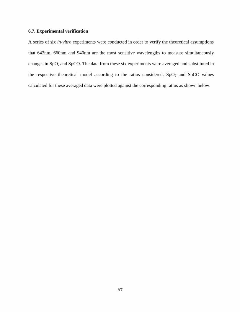
67
6.7. Experimental verification
A series of six in-vitro experiments were conducted in order to verify the theoretical assumptions
that 643nm, 660nm and 940nm are the most sensitive wavelengths to measure simultaneously
changes in SpO2 and SpCO. The data from these six experiments were averaged and substituted in
the respective theoretical model according to the ratios considered. SpO2 and SpCO values
calculated for these averaged data were plotted against the corresponding ratios as shown below.
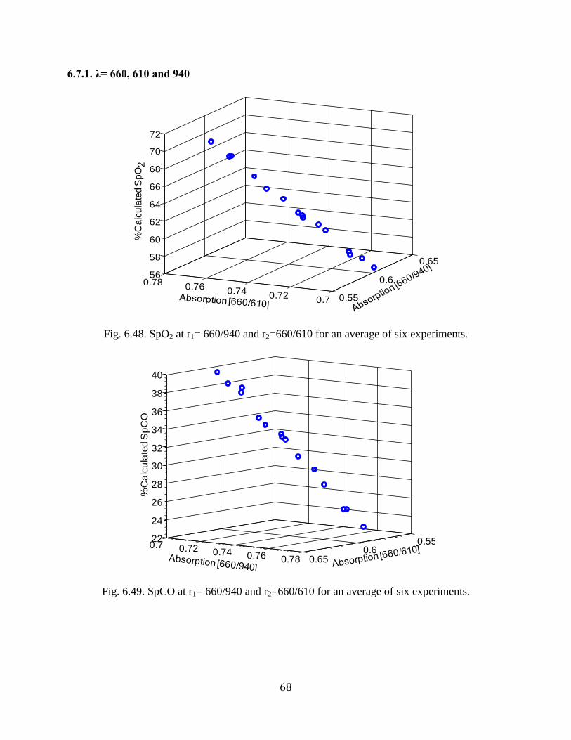
68
6.7.1. λ= 660, 610 and 940
Fig. 6.48. SpO2 at r1= 660/940 and r2=660/610 for an average of six experiments.
Fig. 6.49. SpCO at r1= 660/940 and r2=660/610 for an average of six experiments.
0.55
0.6
0.65
0.70.72
0.740.76
0.7856
58
60
62
64
66
68
70
72%
Ca
lcu
late
d S
pO
2
0.550.6
0.65
0.7 0.72 0.74 0.76 0.78
22
24
26
28
30
32
34
36
38
40
%C
alc
ula
ted
Sp
CO
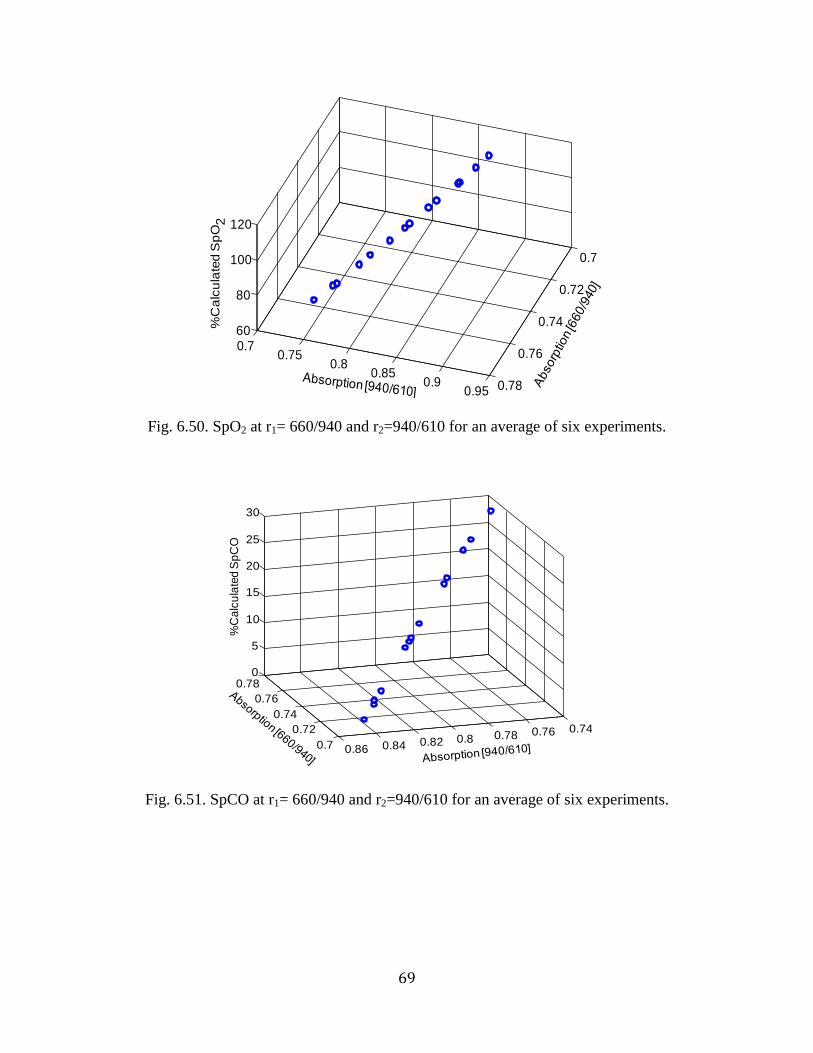
69
Fig. 6.50. SpO2 at r1= 660/940 and r2=940/610 for an average of six experiments.
Fig. 6.51. SpCO at r1= 660/940 and r2=940/610 for an average of six experiments.
0.7
0.72
0.74
0.76
0.78
0.70.75
0.80.85
0.90.95
60
80
100
120%
Ca
lcu
late
d S
pO
2
0.7
0.72
0.74
0.76
0.78
0.740.760.780.80.820.840.86
0
5
10
15
20
25
30
%C
alc
ula
ted
Sp
CO
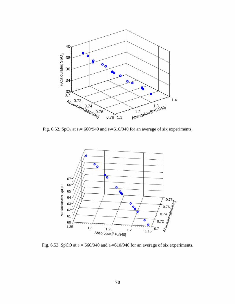
70
Fig. 6.52. SpO2 at r1= 660/940 and r2=610/940 for an average of six experiments.
Fig. 6.53. SpCO at r1= 660/940 and r2=610/940 for an average of six experiments.
0.7
0.72
0.74
0.76
0.78 1.1
1.2
1.3
1.4
32
34
36
38
40
%C
alc
ula
ted
Sp
O2
0.7
0.72
0.74
0.76
0.78
1.151.21.251.31.35
60
61
62
63
64
65
66
67
%C
alc
ula
ted
Sp
CO
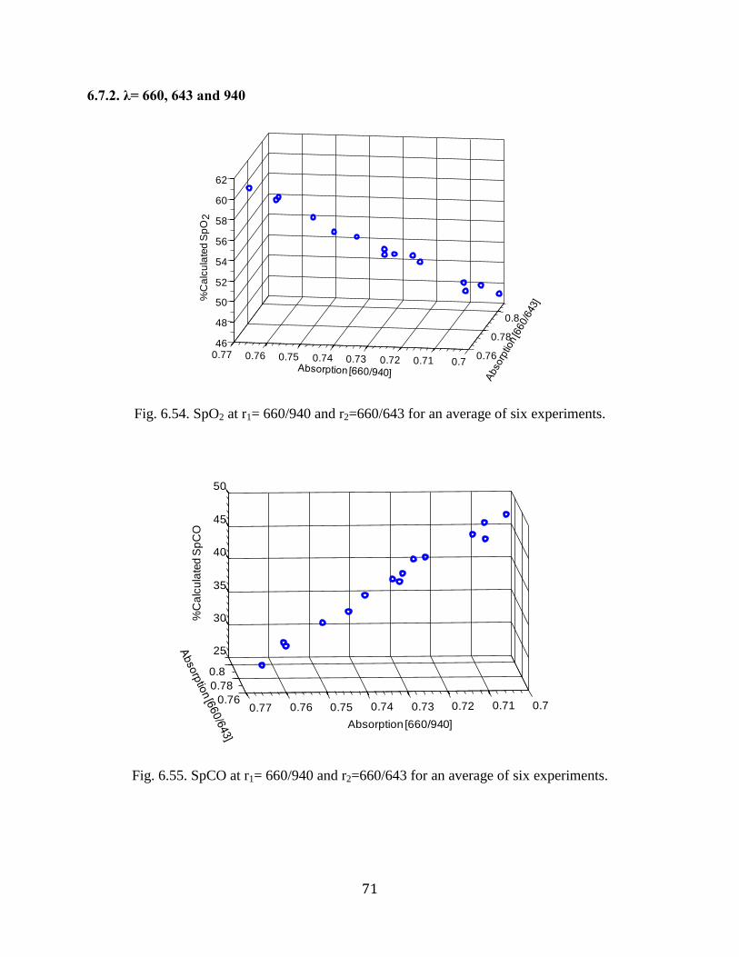
71
6.7.2. λ= 660, 643 and 940
Fig. 6.54. SpO2 at r1= 660/940 and r2=660/643 for an average of six experiments.
Fig. 6.55. SpCO at r1= 660/940 and r2=660/643 for an average of six experiments.
0.76
0.78
0.8
0.70.710.720.730.740.750.760.7746
48
50
52
54
56
58
60
62
%C
alc
ula
ted
Sp
O2
0.76
0.78
0.8
0.70.710.720.730.740.750.760.77
25
30
35
40
45
50
Absorption [660/940]
%C
alc
ula
ted
Sp
CO
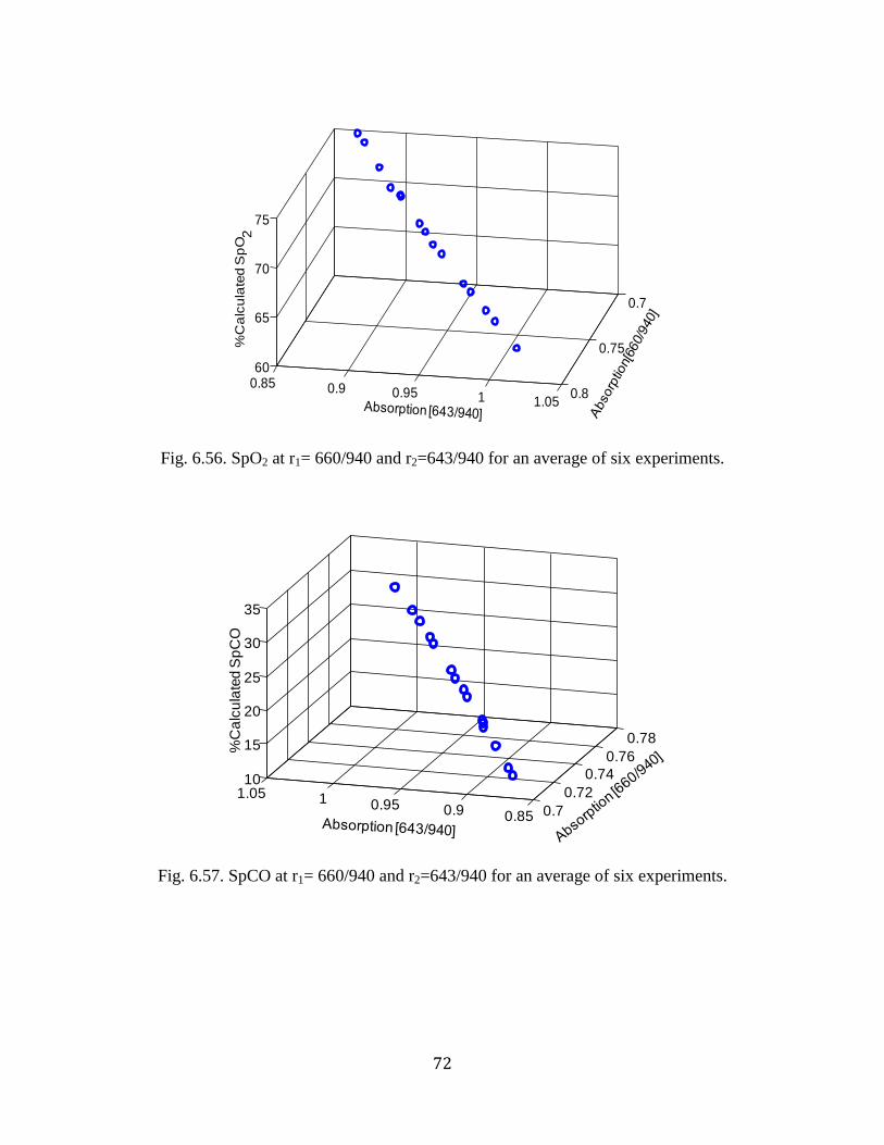
72
Fig. 6.56. SpO2 at r1= 660/940 and r2=643/940 for an average of six experiments.
Fig. 6.57. SpCO at r1= 660/940 and r2=643/940 for an average of six experiments.
0.7
0.75
0.80.85 0.9 0.95 1 1.05
60
65
70
75
%C
alc
ula
ted
Sp
O2
0.7
0.72
0.74
0.76
0.78
0.850.90.9511.0510
15
20
25
30
35
%C
alc
ula
ted
Sp
CO
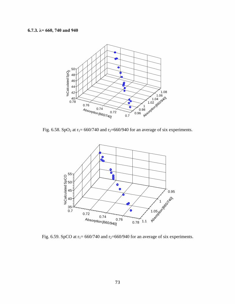
73
6.7.3. λ= 660, 740 and 940
Fig. 6.58. SpO2 at r1= 660/740 and r2=660/940 for an average of six experiments.
Fig. 6.59. SpCO at r1= 660/740 and r2=660/940 for an average of six experiments.
0.960.98
11.02
1.041.06
1.08
0.70.72
0.740.76
0.7840
42
44
46
48
50%
Ca
lcu
late
d S
pO
2
0.95
1
1.05
1.1
0.70.72
0.740.76
0.78
35
40
45
50
55
%C
alc
ula
ted
Sp
CO
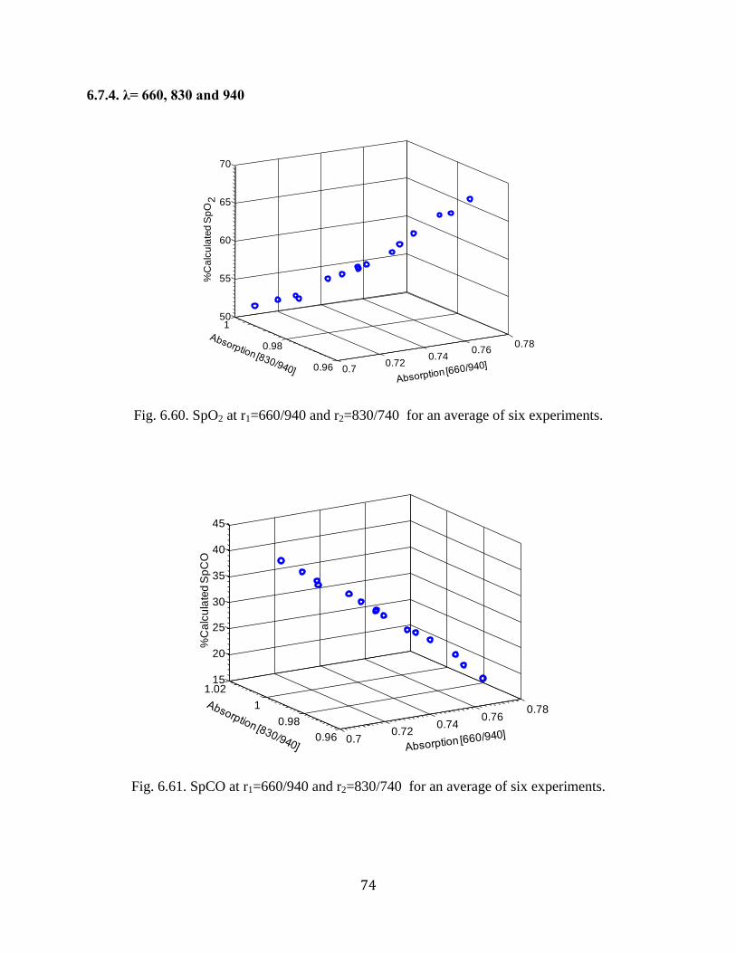
74
6.7.4. λ= 660, 830 and 940
Fig. 6.60. SpO2 at r1=660/940 and r2=830/740 for an average of six experiments.
Fig. 6.61. SpCO at r1=660/940 and r2=830/740 for an average of six experiments.
0.70.72
0.740.76
0.78
0.96
0.98
150
55
60
65
70
%C
alc
ula
ted
Sp
O2
0.70.72
0.740.76
0.78
0.96
0.98
1
1.0215
20
25
30
35
40
45
%C
alc
ula
ted
Sp
CO
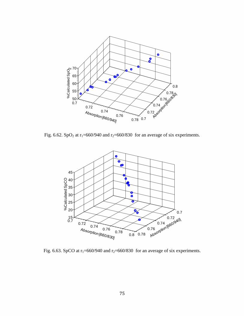
75
Fig. 6.62. SpO2 at r1=660/940 and r2=660/830 for an average of six experiments.
Fig. 6.63. SpCO at r1=660/940 and r2=660/830 for an average of six experiments.
0.70.72
0.740.76
0.78 0.7
0.72
0.74
0.76
0.78
0.8
50
55
60
65
70%
Ca
lcu
late
d S
pO
2
0.7
0.72
0.74
0.76
0.78
0.70.72
0.740.76
0.780.8
15
20
25
30
35
40
45
%C
alc
ula
ted
Sp
CO
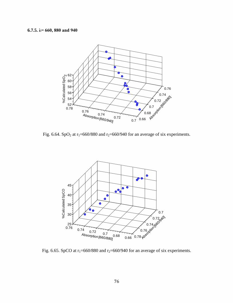
76
6.7.5. λ= 660, 880 and 940
Fig. 6.64. SpO2 at r1=660/880 and r2=660/940 for an average of six experiments.
Fig. 6.65. SpCO at r1=660/880 and r2=660/940 for an average of six experiments.
0.66
0.68
0.7
0.72
0.74
0.76
0.70.72
0.740.76
0.7852
54
56
58
60
62
%C
alc
ula
ted
Sp
O2
0.660.68
0.70.72
0.740.76
0.7
0.72
0.74
0.76
0.78
25
30
35
40
45
%C
alc
ula
ted
Sp
CO
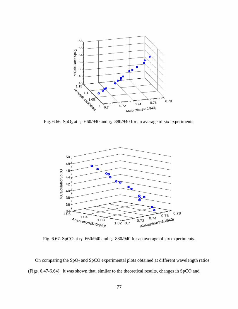
77
Fig. 6.66. SpO2 at r1=660/940 and r2=880/940 for an average of six experiments.
Fig. 6.67. SpCO at r1=660/940 and r2=880/940 for an average of six experiments.
On comparing the SpO2 and SpCO experimental plots obtained at different wavelength ratios
(Figs. 6.47-6.64), it was shown that, similar to the theoretical results, changes in SpCO and
0.70.72
0.740.76
0.78
1
1.05
1.1
1.1546
48
50
52
54
56
58
%C
alc
ula
ted
Sp
O2
0.70.72
0.740.76
0.78
1.021.03
1.041.05
34
36
38
40
42
44
46
48
50
%C
alc
ula
ted
Sp
CO
78
SpO2 (in the presence of HbCO) causes a relatively larger change in the absorption ratios of
660/940 and 643/940 (Fig. 6.53-6.54). Hence, from the theoretical and experimental results, it
was concluded that among the different wavelength ratios considered, absorption ratios at
660/940 and 643/940 has relatively high sensitivity to SpCO and SpO2. Therefore, 660 nm, 643
nm, 940 nm were used to simultaneously measure SpO2 and SpCO.
79
Chapter 7. Algorithm for simultaneous measurement of SpO2 and SpCO
After the specific wavelengths that can be used to measure SpO2 and SpCO have been identified,
the next step was to formulate the algorithm to differentiate between the presence and absence of
HbCO in blood.
To determine HbCO, it is necessary to differentiate between the absorption of blood when
HbCO is present or absent. Hence, the absorptions obtained by our sensor were analyzed in a
series of in-vitro experiments. The absorptions values obtained when HbCO was present were
compared to the absorptions when HbCO was absent. From the results of this comparison, it was
found that apart from 660 nm, 643 nm and 940 nm, the absorption ratios obtained at 740 nm had
a significant change in absorption depending on the presence or absence of HbCO. This can be
explained based on Fig. 2.1, which shows that the absorption in the region between 700 nm to
750 nm decreases when HbCO is present, while the absorption increases when HbCO is absent.
Hence, in addition to 660 nm, 643 nm and 940 nm, the absorption at 740 nm was also included in
the computation to increase the overall selectivity of the device.
These changes in absorption were used in the algorithm to differentiate between the presence
and absence of HbCO. A series of 20 in-vitro experiments with elevated HbCO resulted in
approximately 350 data points at each of the four wavelengths (643 nm, 660 nm, 740 nm, 940
nm). Similarly, a series of 20 in-vitro experiments conducted in the absence of HbCO resulted in
approximately 350 data points at each of the four wavelengths. Based on the absorption values
that were observed from these results, thresholds were set to differentiate between the presence
and absence of HbCO. These thresholds were incorporated into the algorithm to differentiate
between the presence or absence of HbCO.
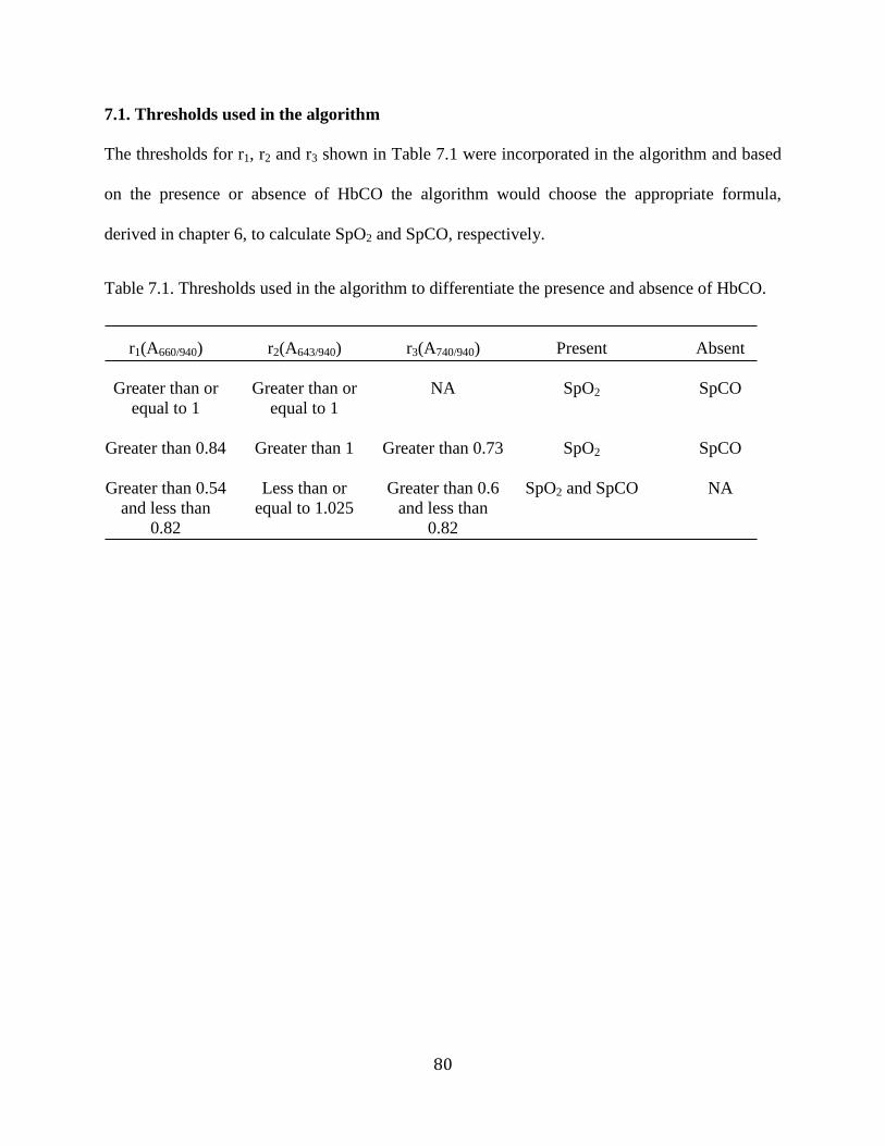
80
7.1. Thresholds used in the algorithm
The thresholds for r1, r2 and r3 shown in Table 7.1 were incorporated in the algorithm and based
on the presence or absence of HbCO the algorithm would choose the appropriate formula,
derived in chapter 6, to calculate SpO2 and SpCO, respectively.
Table 7.1. Thresholds used in the algorithm to differentiate the presence and absence of HbCO.
r1(A660/940)
r2(A643/940)
r3(A740/940)
Present
Absent
Greater than or
equal to 1
Greater than or
equal to 1
NA SpO2 SpCO
Greater than 0.84 Greater than 1 Greater than 0.73 SpO2 SpCO
Greater than 0.54
and less than
0.82
Less than or
equal to 1.025
Greater than 0.6
and less than
0.82
SpO2 and SpCO NA
81
Chapter 8. Algorithm to calculate SpO2 and SpCO
A series of 19 in-vitro SpO2 and SpCO experiments were conducted resulting in 285 and 271
data points, respectively. The absorption values obtained at 643nm, 660nm, 740nm, and 940 nm
were averaged and substituted in the algorithm. SpO2 and SpCO calculated by the algorithm
were plotted against the actual values of SpO2 and SpCO obtained from the IL 682 CO-
Oximeter, respectively. The regression equations obtained for SpO2 and SpCO are shown in Fig.
8.1 and Fig. 8.4. To validate the regression equations, another series of 5 experiments were
conducted resulting in 120 and 117 data points for SpO2 and SpCO, respectively. These data
points were averaged and then calibrated using the regression line obtained from Fig. 8.1 and
8.4. The calibrated results were plotted against the actual values obtained from the IL 682 CO-
Oximeter as shown in Fig. 8.2 and 8.5. Variations in the absorption values were noted, at all
wavelengths, between different experiments even for the same value of SpCO. To compensate
for these variations, which were later determined to be caused by changes in light coupling
between the sensor and tissue simulator, the data points used to calculate and validate the
regression equation were averaged.
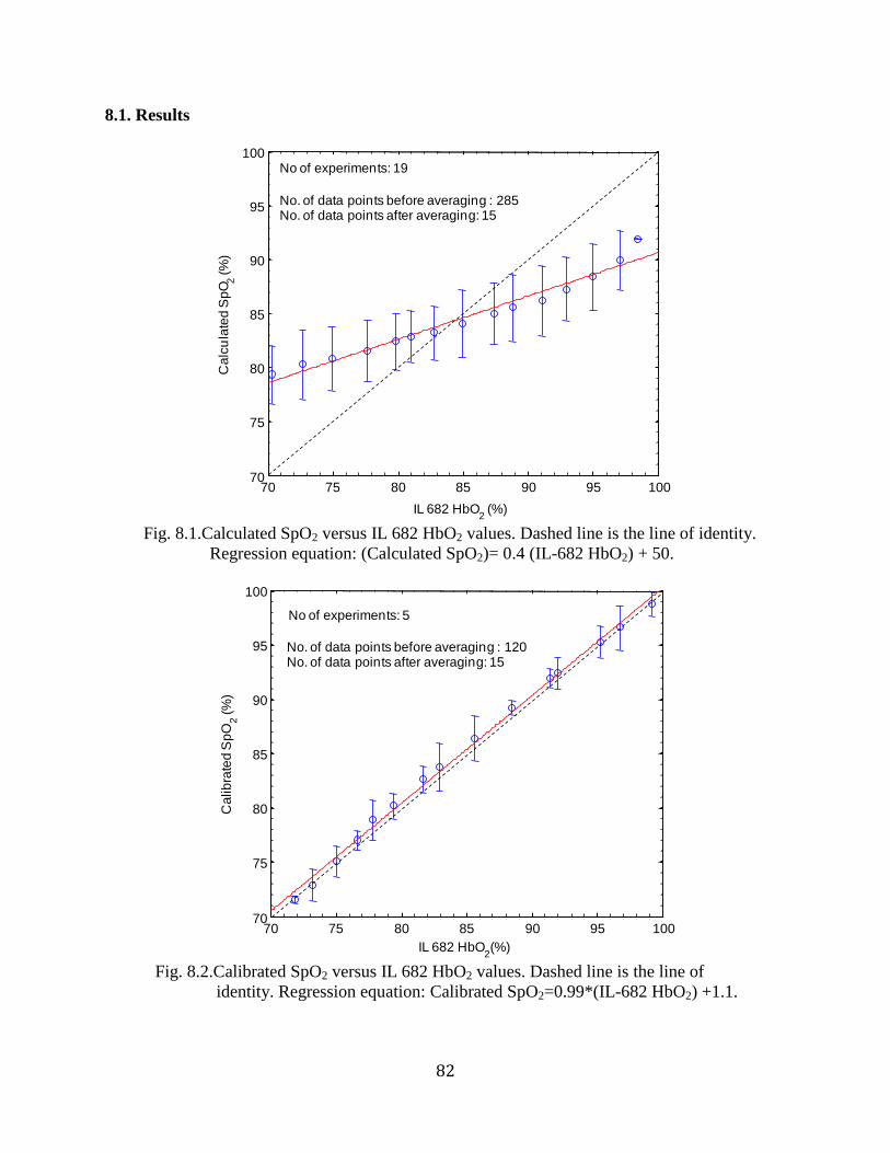
82
8.1. Results
Fig. 8.1.Calculated SpO2 versus IL 682 HbO2 values. Dashed line is the line of identity.
Regression equation: (Calculated SpO2)= 0.4 (IL-682 HbO2) + 50.
Fig. 8.2.Calibrated SpO2 versus IL 682 HbO2 values. Dashed line is the line of
identity. Regression equation: Calibrated SpO2=0.99*(IL-682 HbO2) +1.1.
70 75 80 85 90 95 10070
75
80
85
90
95
100
IL 682 HbO2
(%)
Ca
lcu
late
d S
pO
2(%
)
No of experiments: 19
No. of data points before averaging : 285No. of data points after averaging: 15
70 75 80 85 90 95 10070
75
80
85
90
95
100
IL 682 HbO2(%)
Ca
lib
rate
d S
pO
2(%
)
No of experiments: 5
No. of data points before averaging : 120No. of data points after averaging: 15
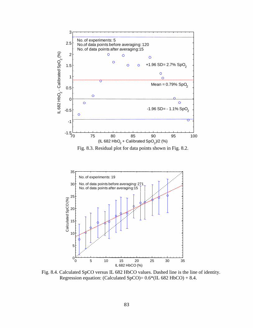
83
Fig. 8.3. Residual plot for data points shown in Fig. 8.2.
Fig. 8.4. Calculated SpCO versus IL 682 HbCO values. Dashed line is the line of identity.
Regression equation: (Calculated SpCO)= 0.6*(IL 682 HbCO) + 8.4.
70 75 80 85 90 95 100-1.5
-1
-0.5
0
0.5
1
1.5
2
2.5
3
(IL 682 HbO2
+ Calibrated SpO2)/2 (%)
IL 6
82
Hb
O2
-C
alib
rate
d S
pO
2(%
)
Mean = 0.79% SpO2
+1.96 SD= 2.7% SpO2
-1.96 SD= - 1.1% SpO2
No. of experiments: 5No.of data points before averaging: 120No. of data points after averaging:15
0 5 10 15 20 25 30 350
5
10
15
20
25
30
35
IL 682 HbCO (%)
Ca
lcu
late
d S
pC
O (%
)
No. of experiments: 19
No. of data points before averaging: 271No. of data points after averaging:15
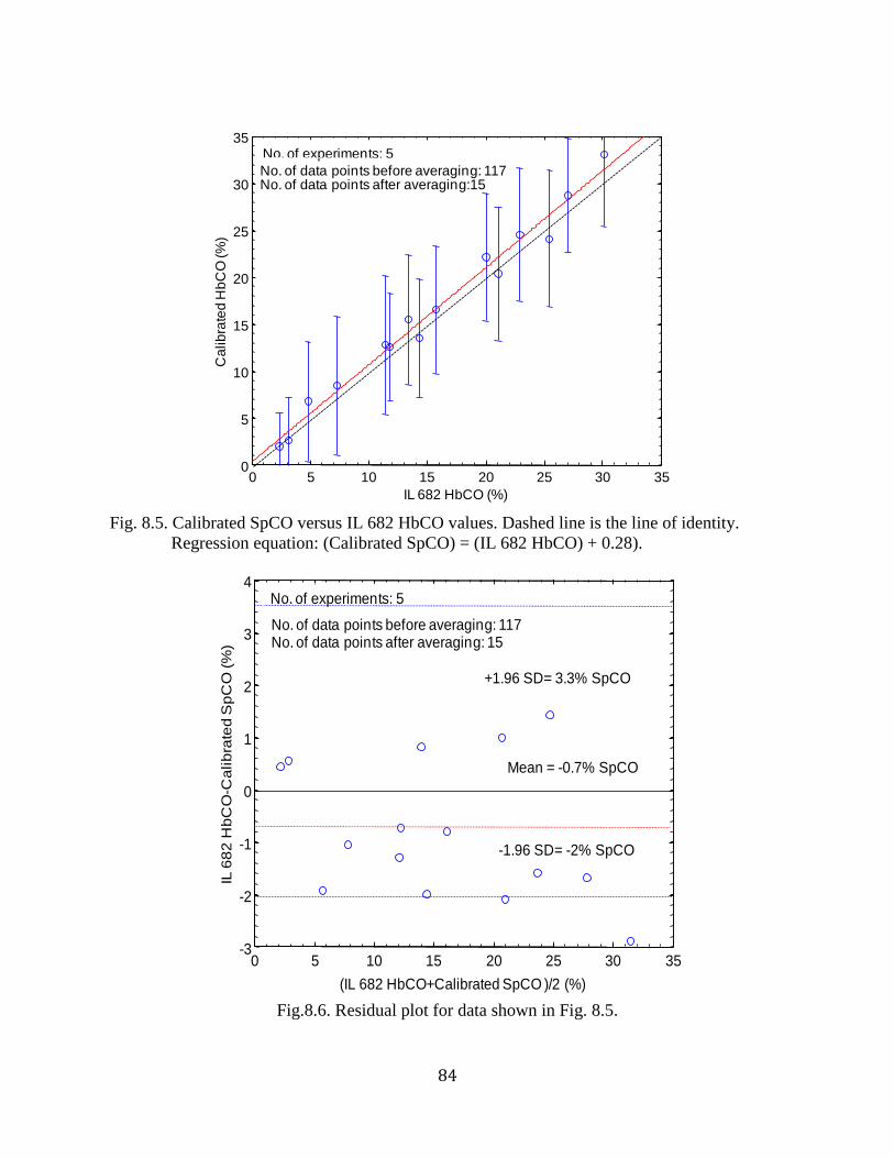
84
Fig. 8.5. Calibrated SpCO versus IL 682 HbCO values. Dashed line is the line of identity.
Regression equation: (Calibrated SpCO) = (IL 682 HbCO) + 0.28).
Fig.8.6. Residual plot for data shown in Fig. 8.5.
0 5 10 15 20 25 30 350
5
10
15
20
25
30
35
IL 682 HbCO (%)
Ca
lib
rate
d H
bC
O (%
)
No. of experiments: 5
No. of data points before averaging: 117No. of data points after averaging:15
0 5 10 15 20 25 30 35-3
-2
-1
0
1
2
3
4
(IL 682 HbCO+Calibrated SpCO )/2 (%)
IL 6
82
Hb
CO
-Ca
lib
rate
d S
pC
O (
%)
+1.96 SD= 3.3% SpCO
Mean = -0.7% SpCO
No. of data points before averaging: 117No. of data points after averaging: 15
No. of experiments: 5
-1.96 SD= -2% SpCO
85
8.2. Discussion
Comparing Fig. 8.1 to Fig. 8.2, it is evident that the variation between the calibrated SpO2 and
IL-682 reference values were much smaller compared to the variation between the calculated
SpO2 and IL-682 reference readings. Similarly, the variation between the calibrated SpCO and
IL 682 CO-oximeter readings (Fig. 8.5) was smaller than the variation between the calculated
SpCO and IL 682 HbCO (Fig. 8.4). From Fig. 8.1 and Fig. 8.2, it is also evident that the
variations observed between individual experiments, indicated by the error bars, were
approximately 3% for SpO2 before calibration, but was smaller for the calibrated SpO2 values.
From Fig. 8.4 and 8.5, it was observed that the variations between individual experiments were
more pronounced in SpCO experiments, at approximately 6%, for both calculated and
calibrated values.
Results from SpCO experiments were analyzed to determine if blood hematocrit (HCT)
levels caused the variations observed between the experiments. It was observed that calculated
values from two SpCO experiments with the same HCT level at approximately 30% had a
standard deviation of ± 2% and ± 7%, respectively. Similarly, it was also observed that results
from another set of two SpCO experiments with different HCT levels at approximately 40% and
30% had a similar standard deviation of ± 2.9% and ± 3.1%, respectively. Hence, it was
concluded that changes in HCT levels did not have a significant effect on the results. Hence,
steady state SpCO experiments were conducted to determine if changes in light coupling caused
large variations between the SpCO obtained from different experiments. These experiments were
conducted by maintaining HbCO level at a steady state value. Other variables like the blood
hematocrit were also held constant and readings from our sensor were obtained along with
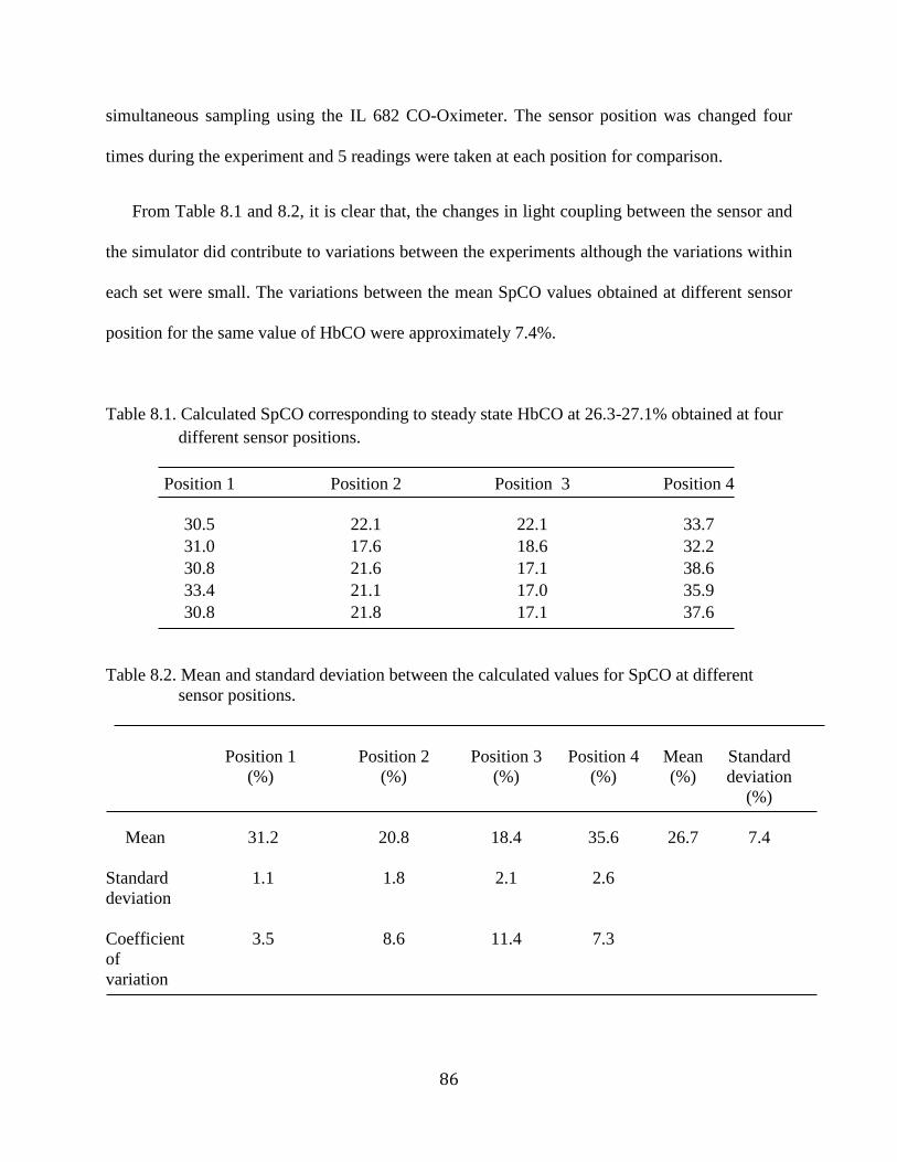
86
simultaneous sampling using the IL 682 CO-Oximeter. The sensor position was changed four
times during the experiment and 5 readings were taken at each position for comparison.
From Table 8.1 and 8.2, it is clear that, the changes in light coupling between the sensor and
the simulator did contribute to variations between the experiments although the variations within
each set were small. The variations between the mean SpCO values obtained at different sensor
position for the same value of HbCO were approximately 7.4%.
Table 8.1. Calculated SpCO corresponding to steady state HbCO at 26.3-27.1% obtained at four
different sensor positions.
Position 1
Position 2 Position 3 Position 4
30.5 22.1 22.1 33.7
31.0 17.6 18.6 32.2
30.8 21.6 17.1 38.6
33.4 21.1 17.0 35.9
30.8 21.8 17.1 37.6
Table 8.2. Mean and standard deviation between the calculated values for SpCO at different
sensor positions.
Position 1
(%)
Position 2
(%)
Position 3
(%)
Position 4
(%)
Mean
(%)
26.7
Standard
deviation
(%)
7.4 Mean 31.2 20.8 18.4 35.6
Standard
deviation
1.1 1.8 2.1 2.6
Coefficient
of
variation
3.5 8.6 11.4 7.3
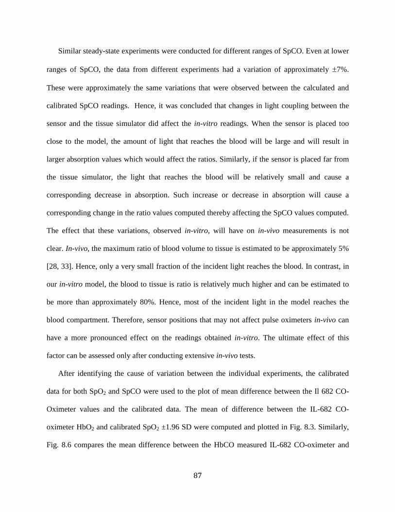
87
Similar steady-state experiments were conducted for different ranges of SpCO. Even at lower
ranges of SpCO, the data from different experiments had a variation of approximately 7%.
These were approximately the same variations that were observed between the calculated and
calibrated SpCO readings. Hence, it was concluded that changes in light coupling between the
sensor and the tissue simulator did affect the in-vitro readings. When the sensor is placed too
close to the model, the amount of light that reaches the blood will be large and will result in
larger absorption values which would affect the ratios. Similarly, if the sensor is placed far from
the tissue simulator, the light that reaches the blood will be relatively small and cause a
corresponding decrease in absorption. Such increase or decrease in absorption will cause a
corresponding change in the ratio values computed thereby affecting the SpCO values computed.
The effect that these variations, observed in-vitro, will have on in-vivo measurements is not
clear. In-vivo, the maximum ratio of blood volume to tissue is estimated to be approximately 5%
[28, 33]. Hence, only a very small fraction of the incident light reaches the blood. In contrast, in
our in-vitro model, the blood to tissue is ratio is relatively much higher and can be estimated to
be more than approximately 80%. Hence, most of the incident light in the model reaches the
blood compartment. Therefore, sensor positions that may not affect pulse oximeters in-vivo can
have a more pronounced effect on the readings obtained in-vitro. The ultimate effect of this
factor can be assessed only after conducting extensive in-vivo tests.
After identifying the cause of variation between the individual experiments, the calibrated
data for both SpO2 and SpCO were used to the plot of mean difference between the Il 682 CO-
Oximeter values and the calibrated data. The mean of difference between the IL-682 CO-
oximeter HbO2 and calibrated SpO2 ±1.96 SD were computed and plotted in Fig. 8.3. Similarly,
Fig. 8.6 compares the mean difference between the HbCO measured IL-682 CO-oximeter and
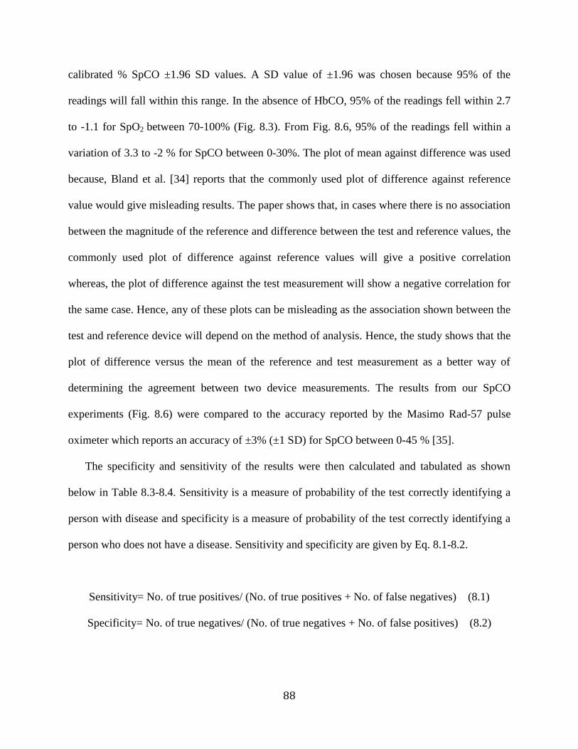
88
calibrated % SpCO ±1.96 SD values. A SD value of ±1.96 was chosen because 95% of the
readings will fall within this range. In the absence of HbCO, 95% of the readings fell within 2.7
to -1.1 for SpO2 between 70-100% (Fig. 8.3). From Fig. 8.6, 95% of the readings fell within a
variation of 3.3 to -2 % for SpCO between 0-30%. The plot of mean against difference was used
because, Bland et al. [34] reports that the commonly used plot of difference against reference
value would give misleading results. The paper shows that, in cases where there is no association
between the magnitude of the reference and difference between the test and reference values, the
commonly used plot of difference against reference values will give a positive correlation
whereas, the plot of difference against the test measurement will show a negative correlation for
the same case. Hence, any of these plots can be misleading as the association shown between the
test and reference device will depend on the method of analysis. Hence, the study shows that the
plot of difference versus the mean of the reference and test measurement as a better way of
determining the agreement between two device measurements. The results from our SpCO
experiments (Fig. 8.6) were compared to the accuracy reported by the Masimo Rad-57 pulse
oximeter which reports an accuracy of ±3% (±1 SD) for SpCO between 0-45 % [35].
The specificity and sensitivity of the results were then calculated and tabulated as shown
below in Table 8.3-8.4. Sensitivity is a measure of probability of the test correctly identifying a
person with disease and specificity is a measure of probability of the test correctly identifying a
person who does not have a disease. Sensitivity and specificity are given by Eq. 8.1-8.2.
Sensitivity= No. of true positives/ (No. of true positives + No. of false negatives) (8.1)
Specificity= No. of true negatives/ (No. of true negatives + No. of false positives) (8.2)
89
where, true positives are cases the device correctly identifies a disease;
true negatives are cases the device correctly identifies a lack of disease;
false positives are the cases the device wrongly identifies a healthy person as having a
disease;
false negatives are the cases the device fails to identify a disease and wrongly identifies a
person with a disease as being healthy [36].
In our case, sensitivity would mean the probability of the device correctly detecting CO
poisoning and specificity is the ability of the device to correctly identify persons who do not
suffer from CO poisoning. For the calculation of SpO2 sensitivity and specificity for, 90% was
considered the threshold for mild hypoxia [37]. In case of SpCO, 12% was considered as the
threshold for calculating specificity and sensitivity because the treatment for carbon monoxide
poisoning is the same for values of SpCO less than 12%. Concentration of SpCO higher than
12% requires specific treatment like 100% oxygen therapy [38].
Table 8.3. Performance characteristics for SpO2 measurements obtained from the in-vitro
model and our sensor using our algorithm.
SpO2
Laboratory
value
<90
Laboratory
value
>90
Total
Negative
Test
Positive
Test
Specificity
83.3%
Sensitivity
100%
Tissue
simulator
<90
9
1
10
True
negative
5
False
negative
0
True
positive
9
False
positive
1
Tissue
simulator
>90
0
5
5
Total
9
6
15
In the experiments we conducted, SpO2 in blood was less than 90% in nine readings and the
algorithm correctly identified all nine cases. Hence, in Table 8.3, the number of true positives is
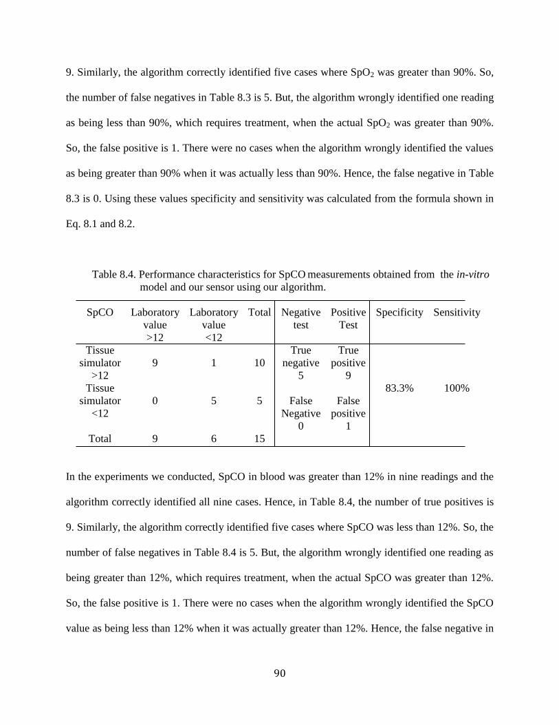
90
9. Similarly, the algorithm correctly identified five cases where SpO2 was greater than 90%. So,
the number of false negatives in Table 8.3 is 5. But, the algorithm wrongly identified one reading
as being less than 90%, which requires treatment, when the actual SpO2 was greater than 90%.
So, the false positive is 1. There were no cases when the algorithm wrongly identified the values
as being greater than 90% when it was actually less than 90%. Hence, the false negative in Table
8.3 is 0. Using these values specificity and sensitivity was calculated from the formula shown in
Eq. 8.1 and 8.2.
Table 8.4. Performance characteristics for SpCO measurements obtained from the in-vitro
model and our sensor using our algorithm.
SpCO
Laboratory
value
>12
Laboratory
value
<12
Total
Negative
test
Positive
Test
Specificity
83.3%
Sensitivity
100%
Tissue
simulator
>12
9
1
10
True
negative
5
False
Negative
0
True
positive
9
False
positive
1
Tissue
simulator
<12
0
5
5
Total
9
6
15
In the experiments we conducted, SpCO in blood was greater than 12% in nine readings and the
algorithm correctly identified all nine cases. Hence, in Table 8.4, the number of true positives is
9. Similarly, the algorithm correctly identified five cases where SpCO was less than 12%. So, the
number of false negatives in Table 8.4 is 5. But, the algorithm wrongly identified one reading as
being greater than 12%, which requires treatment, when the actual SpCO was greater than 12%.
So, the false positive is 1. There were no cases when the algorithm wrongly identified the SpCO
value as being less than 12% when it was actually greater than 12%. Hence, the false negative in
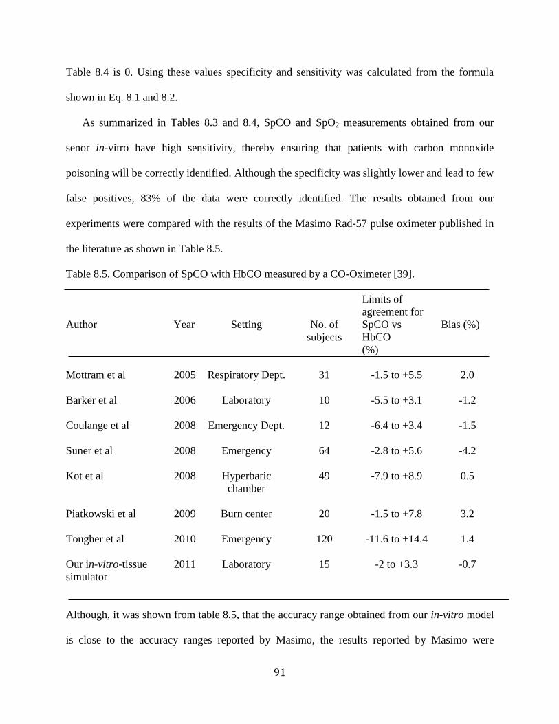
91
Table 8.4 is 0. Using these values specificity and sensitivity was calculated from the formula
shown in Eq. 8.1 and 8.2.
As summarized in Tables 8.3 and 8.4, SpCO and SpO2 measurements obtained from our
senor in-vitro have high sensitivity, thereby ensuring that patients with carbon monoxide
poisoning will be correctly identified. Although the specificity was slightly lower and lead to few
false positives, 83% of the data were correctly identified. The results obtained from our
experiments were compared with the results of the Masimo Rad-57 pulse oximeter published in
the literature as shown in Table 8.5.
Table 8.5. Comparison of SpCO with HbCO measured by a CO-Oximeter [39].
Author
Year
Setting
No. of
subjects
Limits of
agreement for
SpCO vs
HbCO
(%)
Bias (%)
Mottram et al
2005
Respiratory Dept.
31
-1.5 to +5.5
2.0
Barker et al
2006
Laboratory
10
-5.5 to +3.1
-1.2
Coulange et al
2008
Emergency Dept.
12
-6.4 to +3.4
-1.5
Suner et al
2008
Emergency
64
-2.8 to +5.6
-4.2
Kot et al
2008
Hyperbaric
chamber
49
-7.9 to +8.9
0.5
Piatkowski et al
2009
Burn center
20
-1.5 to +7.8
3.2
Tougher et al
2010
Emergency
120
-11.6 to +14.4
1.4
Our in-vitro-tissue
simulator
2011
Laboratory
15
-2 to +3.3
-0.7
Although, it was shown from table 8.5, that the accuracy range obtained from our in-vitro model
is close to the accuracy ranges reported by Masimo, the results reported by Masimo were
92
obtained in-vivo whereas our results were obtained from an in-vitro model. Various
physiological parameters like skin color, amount of tissue, vasoconstriction that were not
simulated in our in-vitro model may affect in-vivo measurements. Similarly, factors that are more
pronounced in the model may or may not affect in-vivo measurements. Hence, the results
obtained from our model cannot be ascertained without further in-vivo verifications. Conducting
human studies to simultaneously calculate SpO2 and SpCO using our algorithm is a part of future
work. This would involve identifying the factors that affect the measurement of SpCO and SpO2
in-vivo and compensating for those variations in order to produce accurate in-vivo measurements
using a pulse oximeter.
93
Chapter 9. Conclusions and future work
Measurement of vital physiological conditions from patients is important to provide effective
triage and medical care in the field. Developments in remote non-invasive monitoring of
physiological parameters could provide a possibility of immediate medical care for firefighters,
army personnel and other people working in dangerous environment. SpCO measurement using
a wireless wearable pulse oximeter that measures SpO2, HR and RR would have a significant
advantage and could find potential applications for people who are exposed to CO in their line of
duty. Pulse oximeters are unable to detect HbCO in blood and give erroneous SpO2 values in the
presence of HbCO. This research therefore, was aimed at developing an algorithm for
simultaneous measurement of SpO2 and SpCO using a wireless wearable pulse oximeter
developed in our laboratory.
To simultaneously measure SpO2 and SpCO, a minimum of three wavelengths were required
since it involves computing three unknown variables which includes the concentration of HbO2,
HbCO and Hb. From the absorption spectra of Hb and its derivatives at wavelengths between
600 nm and 1000 nm, several specific wavelengths at which changes in SpO2 and SpCO can be
measured with relatively high sensitivity and specificity were identified. Based on the
availability of LEDs used in the prototype sensor developed in our laboratory, a set of three
wavelengths (643 nm, 660 nm, 940 nm) were identified. To verify this choice of wavelengths, a
theoretical model was developed using the Beer-Lam ert’s law. From theoretical simulations, it
was found that absorption ratios of 660 nm/940 nm and 643 nm/940 nm can be used for
simultaneous measurement of SpO2 and SpCO with relatively high sensitivity. Additionally, an
algorithm was formulated to calculate SpO2 and SpCO simultaneously. Hence, based on the in-
vitro experiments conducted, in addition to 660 nm, 643 nm and 940 nm, absorption at 740 nm
94
was also included to increase the selectivity of the device. Based on a series of in-vitro
preliminary experiments, in addition to 660 nm, 643 nm, and 940 nm, the absorption at 740 nm
was included to increase the selectivity of the device. Based on the results of the in- vitro
experiments, thresholds for the absorption ratios at 660/940. 643/940 and 740/940 were
incorporated to differentiate the presence and absence of HbCO. The last objective of the thesis
was to verify this algorithm using in-vitro experimental results. From a series of in-vitro
experiments conducted, SpO2 and SpCO were calculated using the algorithm. The preliminary
results from our device reports an accuracy of 2.7 to -1.1 for 70-100% SpO2 and 3.3 to -2 % for
0-30% SpCO with a specificity of 83.3% and a sensitivity of 100% for both SpO2 and SpCO,
respectively.
Although the performance characteristics obtained from the in-vitro measurements are within
the clinically acceptable range, we observed variations in SpCO between the experiments. This
was identified to be caused by changes in the coupling of light between the optical reflectance
sensor and the in vitro tissue simulator. The effect that these variations will have on in-vivo
measurements is not clear. Hence, the algorithm developed in-vitro will need to be evaluated in-
vivo by conducting human validation studies. This would involve identifying the factors that
could potentially affect in-vivo measurement of SpCO and SpO2 and compensate for those
variations in order to produce accurate measurements using a wearable pulse oximeter.
In a clinical setting, monitoring of SpO2 is vital for following physiological trends during
surgical procedures, post surgery, in emergency rooms and in intensive care units. On the
contrary, the ability to measure SpCO is more vital for spot checking to diagnose CO poisoning
rather than to monitor a trend. Typically, the presence of SpCO at values greater than 25% can
cause permanent neurological damage. The Masimo Rad 57 pulse oximeter measures SpCO with
95
an accuracy of 3% (1SD). Hence, 1.96 SD which would include 95% of the measurements will
have an accuracy of approximately 6%. Although this is not a high accuracy value, the
indication of HbCO in blood will enable screening of patients with CO poisoning and enable
clinicians to decide on an appropriate course of action. Hence, from a clinical standpoint, spot
checking for SpCO is more critical than the need to monitor the trend in SpCO measurement.
Although, results from our algorithm using data points obtained from an in-vitro simulator have
been shown to have an accuracy of 2.7 to -1.1, variations up to 7% have been observed due to
changes in the coupling of light between the sensor and the simulator. If the coupling of light
between the sensor and the skin is not found to affect the readings in-vivo, and if we can identify
and compensate for other factors that could potentially affect SpCO measurement in-vivo, then
the accuracy rate that can be obtained from our algorithm can potentially be better than the
accuracy of currently available devices.
In-vivo testing of our algorithm can be done in the future similar to the in-vivo testing reported
by Tougher et al. [39] in trauma and burn center of a hospital. People suspected of CO poisoning
were tested using the Masimo device with simultaneous blood sampling using a CO-Oximeter
(Siemens Rapidlab 1200 blood gas analyzer) to obtain the true HbCO values. The results from
both the methods were then compared to assess the accuracy of the Masimo Rad 57 pulse
oximeter. Testing can also be conducted in a laboratory setting using volunteers breathing safe
levels of SpCO. Testing of the Masimo pulse oximeter reported by Barker et al. [40] was
conducted in a laboratory where 10 volunteers breathed 500 ppm of CO until HbCO levels
reached 15%. As the readings from the Masimo device was obtained, blood samples from arterial
cannulas were obtained simultaneously to test for true HbCO values. The readings from the two
devices were compared to establish the accuracy of the Masimo Rad 57 oximeter.
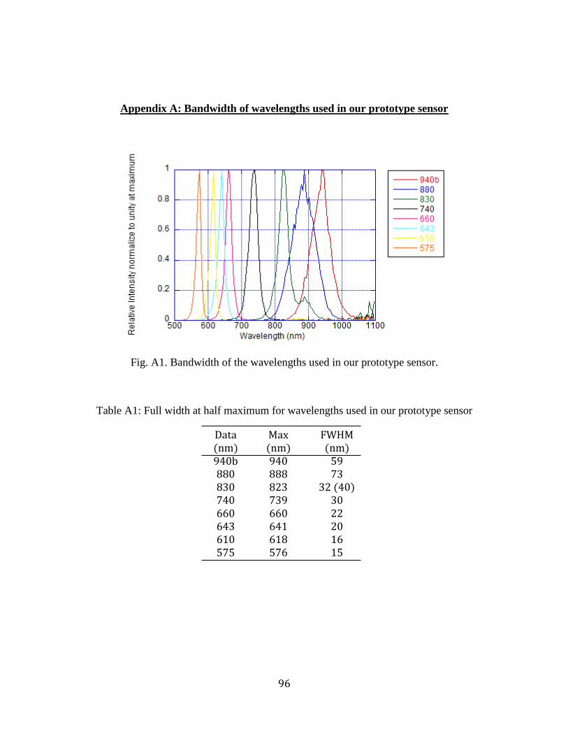
96
Appendix A: Bandwidth of wavelengths used in our prototype sensor
Fig. A1. Bandwidth of the wavelengths used in our prototype sensor.
Table A1: Full width at half maximum for wavelengths used in our prototype sensor
Data (nm)
Max (nm)
FWHM (nm)
940b 940 59 880 888 73 830 823 32 (40) 740 739 30 660 660 22 643 641 20 610 618 16 575 576 15
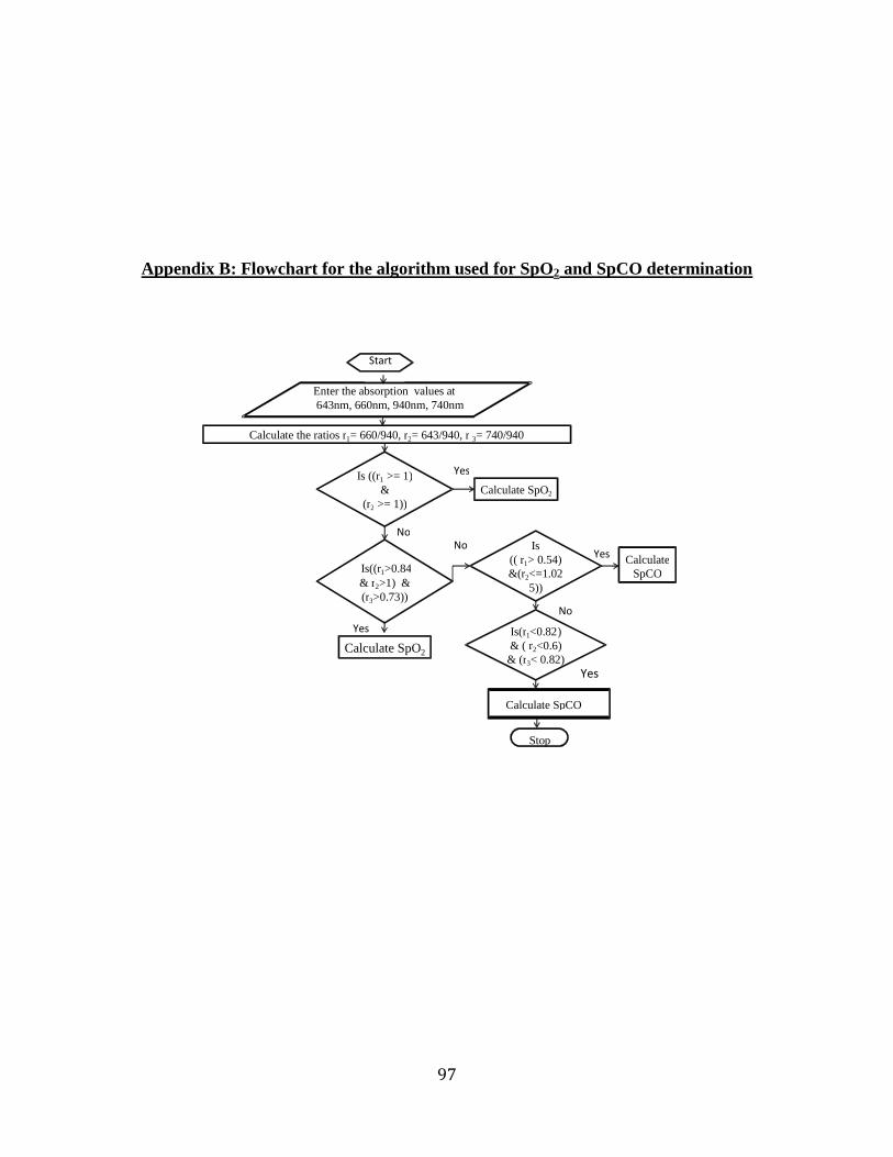
97
Appendix B: Flowchart for the algorithm used for SpO2 and SpCO determination
Calculate the ratios r 1 = 660/940, r 2 = 643/940, r 3 = 740/940
Is ((r 1 >= 1) &
(r 2 >= 1)) Calculate SpO 2
Yes
No
Enter the absorption values at 643nm, 660nm, 940nm, 740nm
Start
Is((r 1 >0.84 & r 2 >1) & (r 3 >0.73))
No Is (( r 1 > 0.54) &(r 2 <=1.02
5))
Yes Calculate
SpCO
Yes Calculate SpO 2
No Is(r 1 <0.82 ) & ( r 2 <0.6)
& (r 3 < 0.82) Yes
Calculate SpCO
Stop
98
REFERENCES:
1. J. G. We ster (Editor), “Design of pulse oximeter”, S. A. Clark (Author), “ Normal
Oxygen Transport”, IOP publishing Ltd, pp.1-13, 1997.
2. A. C. Guyton and J. E. Hall. “Text ook of Medical Physiology”, W.B. Saunders
Company, pp 516-517, 1996.
3. M. F. Perutz. “Hemoglo in structure and respiratory transport”, Sci Am., Vol. 239(6),
pg. 92-125, 1978.
4. J. P. Payne and J. W. Servinghaus, “Pulse oximetry”, Springer-Verlag, pp21-22, 1986.
5. J. G. We ster (Editor), “Design of pulse oximeter,” O. Wie en (author), “Light
a sor ance in pulse oximetry,” IOP pu lishing Ltd, pp. 40-55, 1997.
6. J. G. We ster (Editor), “Design of pulse oximeter”, Joanna B Ruchala (author),
“Applications of pulse oximetry”, IOP pu lishing Ltd, pp. 214-220, 1997.
7. L. W. Kao, K. A. Nanagas, “ Car on monoxide poisoning”, Medical Clinics of North
America, Vol. 89, pp. 1161-1194, 2005.
8. M.Micheal, R.E.Zumwalt, “Fatal car on monoxide poisoning after the detonation of
explosives in an underground mine: A case report”, American Journal of Forensic
Medicine & Pathology, Vol. 22, pp 387-390, 2001.
9. H. Mathew, A. A. H. Lawson, “Car on monoxide poisoning in a former mining
community”, Britsh medical journal, Vol. 286, pp:18-19, 1983.
10. A. Ernst, J. D. Zi rak, “Car on monoxide poisoning”, The New England Journal of
Medicine, Vol. 339, pp. 1603-1609, 2004.
11. D. G. Penny, “Hemodynamic response to car on monoxide”, Environmental Health
Perspectives, Vol(77), pp. 121-30, 1978.
12. B. W. Timothy, C. D. Ridgeley, “Car on monoxide”, R. Zajtchuk, (Editor),
“Occupational health, the soldier and the industrial ase”, pp, 397-429, 1993.
13. Y. Mendelson, “Pulse oximetry: Theory and applications for noninvasive monitoring,”
Clinical Chemistry, Vol. 38, pp. 1801-1807, 1992.
14. J. Sola and O. Chetelat, “Com ination of multiple paths in pulse oximetry: The finger
ring example,” Proceedings of the 29th
Annual International Conference of IEEE EMBS,
pp. 6697-6698, 2007.
15. J. T. B. Moyle, “Pulse Oximetry”, BMJ ooks, Second edition, pp35-36, 1994.
99
16. N. Sta ile, K. Reynolds, “Technological review of pulse oximeter simulators”, Journal
of Clinical Engineering, pp 287-297, 2002.
17. J. H. Sammons, R. L. Coleman, " Journal of occupational medicine; official publication
of industrial medical association, Vol.16, pp. 543-546, 1974.
18. T. Edrich, M. Flaig, R. Knitza, G. Rall, “ Pulse Oximtery: An improved in-vitro model
that reduces blood flow-related artifacts”, IEEE transactions on biomedical engineering,
Vol. 47(3), pp. 338-343, 2000.
19. R. Nijland, H. W. Jongsma, J. G. Nijhuis, B. Oese urg, “Accuracy of fetal pulse
oximetry and pitfalls in measurements”, European Journal of O stetrics and Gynecolog
and Reproductive Biology, Vol. 72 Suppl. 1, pp. S21-S27, 1997.
20. P. B. Batchelder, D. M. Raley, “Maximizing the la oratory setting for test devices and
understanding statistical output in pulse oximeter”, Anesthesia and Analgesia, Vol. 105,
pp S85- S94, 2007.
21. M. Vegfors et. al., “Accuracy of pulse oximetry at various hematocrits and during
haemolysis in an in vitro model”, Medical and Biological Engineering and computing,
Vol. 31, pp. 135-141, 1993.
22. K. J. Reynolds, J. T. B. Moyle, M. K. Sykes, C. E. W. Hahn, “Response of 10 pulse
oximeters to an in-vitro test system”, British journal of anaesthesia, Vol. 68, pp 365-369,
1992.
23. M. Oura, N, Ko ayashi, S. Yamamori, S. Takeda,”Cali ration System for pulse
spectrophotometer using a double-layer pulsation flow cell”, 31st Annula International
Conference of IEEE EMBS, pp 896-899, 2009.
24. L. J. Brown, “A new instrument for simultaneous measurement of total hemoglo in,
%oxyhemoglobin, % carboxyhemoglobin , %methemoglobin and oxygen content in
whole lood”, IEEE transactions on iomedical engineering, Vol. 27, pp. 132-138, 1980.
25. W. G. Zijlstra, A. Buursma and W. P. Meeuwsen-der Roest, “ A sorption spectra of
human fetal and adult oxyhemoglo in, car oxyhemoglo in and methemoglo in,”
Clinical Chemistry, Vol. 39, pp 1633-1638, 1991
26. V.Twersky, “A sorption and multiple scattering y iological suspensions”, Journal of
the opical society of America, Vol. 60, pp. 1084-1093, 1970.
100
27. J. L. Reuss, “Multilayer modeling of reflectance pulse oximetry”, IEEE transactions on
biomedical engineering, Vol. 52, pp 153-160, 2005.
28. J. M. Schmitt, “Simple photon diffusion analysis of the effects of multiple scattering on
pulse oximetry”, IEEE transactions on iomedical engineering, Vol. 38, pp. 1191-1203,
1991.
29. V. O. Ry nyok, P. A. Kyriacon. “Beer-Lambert law along non-linear mean light
pathways for the rational analysis of photoplethysmography”, Journal of physics:
Conference series 238, pp. 1-7, 2010.
30. P. D. Mannheimer, “The light interaction of pulse oximetry”, Anesthesia and Analgesia,
Vol. 105, pp.10-17, 2006.
31. J. C. S. Lee, P. W. Cheung, D. R. Mar le, M. A. Kenny and D. Landicho, “Simultaneous
measurement of percent car oxyhemoglo in and functional oxygen saturation”, IEEE
Engineering in Medicine and Biological Society 11th
Annual International Conference,
pp. 1092 – 1093, 1989.
32. C. Pieralli, R. Devillers, G. Tri illon, “Three wavelength optical oximetry including the
measurement of car oxyhemoglo in concentration,” Medical Sensors II and fi er
optical sensors, SPIE Vol. 2331, pp. 80-88, 1994.
33. D. R. Marble, D. H. Burns, “Diffusion-based model of pulse oximetry: in vitro and in
vivo comparisons”, Journal of Applied Optics, Vol. 33, pp. 1279-1285, 1994.
34. J. M. Bland, D. G. Altman, “Comparing methods of measurements: why plotting
difference against standard method is misleading”, Lancet, Vol. 346, pp. 1085-7, 1986.
35. Masimo Corporation website. Rad-57 Pulse CO-oximeter.
36. T. W. Loong, “Understanding sensitivity and specificity with the right side of the
rain”, British Medical Journal, Vol 327, pp. 716, 2003.
37. W. W. Lee, K. Mayberry, R. Crapo, R. L. Jensen, “ The accuracy of pulse oximetry in
the emergency department”, American Journal of Emergency Medicine, Volume 18 (4),
pp. 427-431, 2000.
38. N. Hampson (Author), D. G. Penny (Editor) “Car on monoxide poisoning, CRC press,
Chapter 33, pp-739-745, 2008.

101
39. M. Touger, A. Birn aum, J. Wang, K. Chou, D. Pearson, P. Bijur, “Performance of the
RAD-57 Pulse Co-Oximeter compared with standard laboratory carboxyhemoglobin
measurement”, Annals of emergency medicine, Vol 56(4), pp. 382-388, 2010.
40. S. J. Barker, J. Curry, D. Redford, S. Morgan, “Measurement of car oxyhemoglo in and
methemoglo in in pulse oximetry”, Anesthesiology, Vol. 105, pp 892-897, 2006.