ii - ETD - Electronic Theses & Dissertationsetd.library.vanderbilt.edu/.../unrestricted/luhmann-dissertation.pdfno-confounding assumption (see Hagmeyer & Waldmann, 2004; Luhmann, 2005;

BUCKLE: A MODEL OF CAUSAL LEARNING

by

Christian C. Luhmann

Dissertation

Submitted to the Faculty of the

Graduate School of Vanderbilt University

in partial fulfillment of the requirements

for the degree of

DOCTOR OF PHILOSOPHY

in

Psychology

May, 2006

Nashville, Tennessee

Approved:

Woo-kyoung Ahn

Thomas Palmeri

Gordon Logan

David Noelle

ii

To my parents.

iii

ACKNOWLEDGEMENTS

This work has been inspired and supported by a large number of people in my

life. I am grateful for the intellectual, emotional, and financial support provided to me by

my advisor Woo-kyoung Ahn. Throughout our collaboration, she has continually

challenged me to accomplish more than I thought possible. The best example of this is

the project presented here, which began as an odd curiosity and evolved into the large

theoretical statement outlined in these pages.

I would also like to thank the members of my committee: Thomas Palmeri,

Gordon Logan, and David Noelle. These individuals have continually provided me with

useful and thought-provoking feedback that continues to help me improve as both a

researcher and a member of the academic community.

My friends have both provided intellectual stimulation and helped sustain the

motivation necessary to reach my goals. I would like to thank my fellow lab members as

well as friends and colleagues at both Vanderbilt and Yale.

Lastly, I would like to thank my family. My parents’ enthusiasm often seemed

greater than my own and reminded me that I was actually accomplishing something.

Most importantly, I have to thank Heather. Her support, understanding, and willingness

to sacrifice have been infinitely generous and I would not be where I am without her.

iv

TABLE OF CONTENTS

Page

DEDICATION................................................................................................................ii

ACKNOWLEDGEMENTS............................................................................................iii

LIST OF TABLES ........................................................................................................vii

LIST OF FIGURES......................................................................................................xiii

Chapter

I. INTRODUCTION ...............................................................................................1

The Importance and Difficulty of Understanding Alternative Causes ...................1Are Details about Unobserved Alternative Causes Necessary?.............................3

II. EVALUTATING UNOBSERVED CAUSES ......................................................5

Experiment 1 .......................................................................................................5Method.....................................................................................................5

Participants ...................................................................................5Materials and Procedure ...............................................................6

Predictions of ΔP-based Models ...............................................................8Results and Discussion .............................................................................9

III. BUCKLE........................................................................................................... 12

Formal Description of BUCKLE........................................................................ 13Step 1: Inference of Unobserved Cause .................................................. 13Step 2: Learning Algorithm.................................................................... 16

Simulation of BUCKLE..................................................................................... 18Observed Cause Learning....................................................................... 18Unobserved Cause Learning................................................................... 21

Effect of P(u|o,e) on qu................................................................ 21Effects of values of o and e on qu ................................................ 22Effects of qu and qo on P(u|o,e).................................................... 27

Summary................................................................................................ 28

IV. ALTERNATIVE MODELS............................................................................... 29

Constraint-satisfaction Networks ....................................................................... 29

v

The Rescorla-Wagner Model ............................................................................. 32

V. EMPIRICAL TESTS OF THE MODELS .......................................................... 34

Experiment 2 ..................................................................................................... 34Method................................................................................................... 37

Participants ................................................................................. 37Materials and Design .................................................................. 37Procedure ................................................................................... 38

Results and Discussion ........................................................................... 39Experiment 2A ........................................................................... 39

Simulating Experiment 2A with BUCKLE...................... 41Experiment 2B............................................................................ 42

Simulating with the Constraint-satisfaction Model .......... 44Simulating with RW........................................................ 46

Experiment 3 ..................................................................................................... 47Method................................................................................................... 48Results and Discussion ........................................................................... 49Summary................................................................................................ 50

Experiment 4: Judging a Constant Cause ........................................................... 51Method................................................................................................... 52


Results ................................................................................................... 53Experiment 5: Evaluating Beliefs about the Occurrence of Unobserved Causes . 55

Method................................................................................................... 57Participants ................................................................................. 57Materials and Procedure ............................................................. 57

Results ................................................................................................... 58Simulating with BUCKLE...................................................................... 63Summary................................................................................................ 66

Experiment 6: Manipulating Causal Role ........................................................... 67Method................................................................................................... 71


Results ................................................................................................... 75Experiment 7: Order-effects............................................................................... 77

Method................................................................................................... 79Participants ................................................................................. 76Materials..................................................................................... 76Design and Procedure ................................................................. 76

Results and Discussion ........................................................................... 80Experiment 8: The Influence of

€

OE Observations ............................................. 82Method................................................................................................... 84

vi

Participants ................................................................................. 84Design and Procedure ................................................................. 84Stimuli........................................................................................ 86

Results and Discussion ........................................................................... 87Simulating Experiment 8 ........................................................................ 88Summary................................................................................................ 89

VI. GENERAL DISCUSSION................................................................................. 91

The Interchangeable Nature of BUCKLE........................................................... 93Similarity between BUCKLE and Other Models of Learning............................. 96Conclusion....................................................................................................... 100

Appendix

A. LIKELIHOOD COMPUTATIONS FOR BUCKLE......................................... 102

B. LIKELIHOOD COMPUTATIONS FOR MLE ................................................ 108

REFERENCES............................................................................................................ 110

vii

LIST OF TABLES

Table Page

1. The design of Experiment 2 ............................................................................ 35

2. Average trial-by-trial probability judgments from Experiment 4 ..................... 58

viii

LIST OF FIGURES

Figure Page

1. An example contingency table .......................................................................... 2

2. A sample trial illustrating the stimuli from Experiment 1 .................................. 6

3. A summary of the observations using in Experiment 1...................................... 9

4. A illustration of BUCKLE’s two steps ............................................................ 12

5. Simulation results illustrating the influence of P(u|,o,e) on qu.......................... 22

6. Simulation results illustrating qu, qo, and P(u|,o,e) changing over time............. 24

7. Simulation results illustrating the influence of qu and qo on P(u|,o,e) ............... 27

8. Causal strength judgments from Experiment 2A ............................................. 40

9. Confidence judgments from Experiment 2A ................................................... 41

10. Causal strength judgments from Experiment 2B.............................................. 43

11. Confidence judgments from Experiment 2B.................................................... 44

12. Causal strength judgments from Experiment 3 ................................................ 49



15. Participants’ estimates of P(u|,o,e) from Experiment 5 .................................... 61

16. BUCKLE’s estimates of P(u|,o,e) from Experiment 5 ..................................... 65

17. Sample of stimuli used in Experiment 6 .......................................................... 69


19. Design of Experiment 7 .................................................................................. 78


ix

21. Sample of stimuli used in Experiment 8 .......................................................... 85


1

CHAPTER I

INTRODUCTION

This paper presents a new model of causal induction called BUCKLE (Bidirectional

Unobserved Cause LEarning). Existing models of causal induction (e.g. Anderson &

Sheu, 1995; Busemeyer, 1991; Cheng, 1997; Cheng & Novick, 1990, 1992; Dickinson,

Shanks, & Evenden, 1984; Jenkins & Ward, 1965; Schustack & Sternberg, 1981; White,

2002) either ignore or make simplistic assumptions about unobserved causes. In contrast,

BUCKLE makes relatively sophisticated inferences about the occurrence of unobserved

causes in a given situation, which allow unobserved causes to be learned just like

observed causes. As a result, BUCKLE explains learning of not only unobserved but also

observed causes better than existing models of causal induction. Before presenting

BUCKLE, we illustrate why the role of unobserved alternative causes is critical to the

understanding of human causal learning.

The Importance and Difficulty of Understanding Alternative Causes

Current models of causal induction have traditionally assumed that the input

available to reasoners comes in the form of covariation; how the causes vary with their

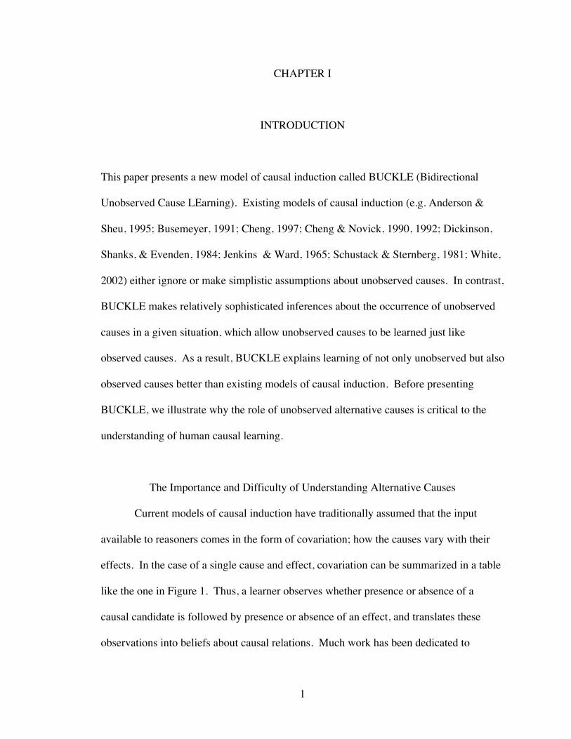
effects. In the case of a single cause and effect, covariation can be summarized in a table

like the one in Figure 1. Thus, a learner observes whether presence or absence of a

causal candidate is followed by presence or absence of an effect, and translates these

observations into beliefs about causal relations. Much work has been dedicated to

2

exploring how this translation is made (see Shanks, Holyoak, & Medin, 1996 for an

extensive review).

Later work, however, has suggested that inferences about one cause may critically

depend on how learners deal with other, alternative causes (e.g., Cheng, Park, Yarlas, &

Holyoak, 1996). For example, Spellman (1996) had participants learn about two liquids

(one red and one blue) and their influence on flowers blooming. When participants were

asked about causal efficacy of the red liquid, their judgments were not simply based on

how the red liquid and blooming covaried. Instead, participants systematically used

observations in which the alternative cause (blue liquid) was held constant (a strategy

referred to as conditionalizing), just as scientists control for potential confounding

variables in experimental design (see also Goodie, Williams, & Crooks, 2003; Waldmann

& Hagmeyer, 2001). Clearly, conditionalizing is advantageous because it prevents

wrongly attributing causal efficacy to a candidate. For instance, upon observing that

more men than women are scientists, one should conditionalize on differences in

Present Absent

Present A B

Absent C D

Cause

Effect

Figure 1 - A contingency table summarizing thecovariation between two binary events. Each cellof the table represents one of the possibleobservations.

3

socialization before concluding genetic differences as the cause (see also Simpson’s

paradox; Simpson, 1951).

Although conditionalizing allows learners to avoid mistaking illusory covariation

as causation, it is often not feasible because it requires alternative to be observed.

Alternative causes can be unobserved because they require special instruments or

methods to be observed (e.g., genetic influences on cancer). More frequently, learners

lack observations about alternative causes simply because they could not possibly

consider all alternative causes of a particular event. Thus, lacking observations about

alternative causes seems to be the rule rather than the exception.

Are Details about Unobserved Alternative Causes Necessary?

One elegant solution to this problem has been proposed in Power PC theory

(Cheng, 1997; see also Pearl, 2000 for a similar approach). The power PC theory

tempers traditional covariation (i.e., ΔP) by performing something analogous to

conditionalizing over a composite of all alternative causes, a. The strength of a is

unknown. However, Cheng (1997) shows that if we assume that a occurs independently

of the target cause, c, that is, P(c|a) = P(c|~a) (henceforth, no-confounding assumption), it

is possible to equate the probability of the effect in the absence of a cause, P(e|~c), with

probability that a is present and causes the effect (see Cheng, 1997 for the proof). Thus,

using P(e|~c), which is computable from observable events, instead of the probability or

strength of a, which are unobserved, these accounts avoid the need to observe alternative

causes.

4

However, recent work has showed that people do not believe that the no-

confounding assumption is required for causal inference. These studies demonstrated

that people are willing to make causal judgments despite acknowledging violations of the

no-confounding assumption (see Hagmeyer & Waldmann, 2004; Luhmann, 2005; and

Experiment 6 in this paper). Then, how do people infer causation from covariation under

confounded situations?

In contrast to the strategy taken by the Power PC theory, several models of causal

induction assume that people learn the causal strength of unobserved causes just like

observed causes (Rescorla & Wagner, 1972; Thagard, 2000). For example, the model

proposed by Rescorla and Wagner (1972) assumes that there is an unobserved cause that

is present on every observation and that this cause accrues associative strength just as

observed causes do. The model that we introduce in this paper, BUCKLE, also assumes

that causal learning involves sophisticated inferences about the probability and strength

of unobserved causes.

In some sense, however, it seems counterintuitive that people would learn without

direct observations. Thus, the first order of business is to determine whether people are

willing to provide judgments of unobserved causes. After establishing people’s

willingness to make judgments about unobserved causes, we will present several

accounts of such judgments, including BUCKLE.

5

CHAPTER II

EVALUATING UNOBSERVED CAUSES

In Experiment 1, participants observed the contingency between one target cause

and one target effect only. They were then asked to judge the causal strength of the target

cause as well as one alternative, unobserved cause. Participants were told that if they

were unable to evaluate a cause, they should provide a response of “N/A” (i.e., not

applicable). Experiment 1 also varied the number of unobserved causes to examine

whether an increased number of unobserved, alternative causes would influence

willingness to make causal judgments.

Experiment 1

Method

Participants

Twenty Vanderbilt University undergraduates participated for partial fulfillment

of course credit.

6

Materials and Procedure

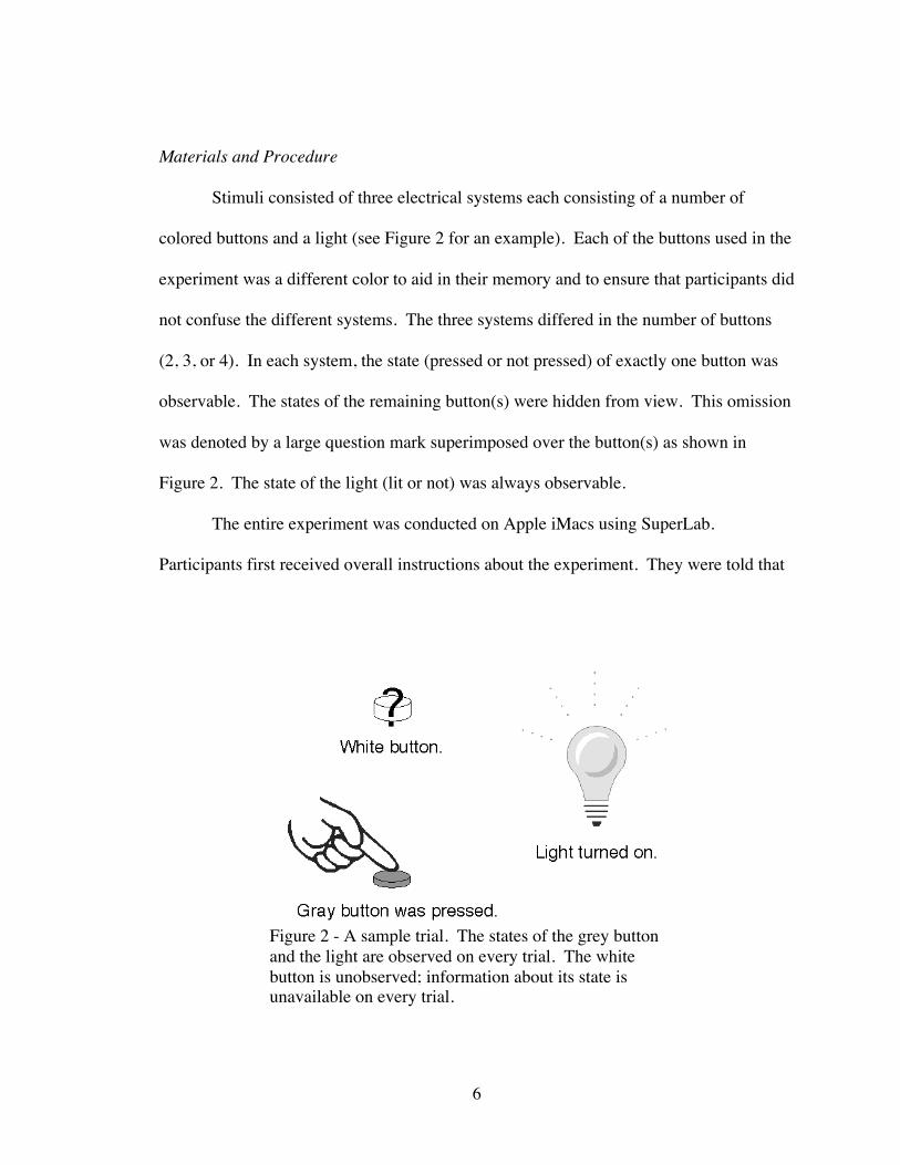
Stimuli consisted of three electrical systems each consisting of a number of

colored buttons and a light (see Figure 2 for an example). Each of the buttons used in the

experiment was a different color to aid in their memory and to ensure that participants did

not confuse the different systems. The three systems differed in the number of buttons

(2, 3, or 4). In each system, the state (pressed or not pressed) of exactly one button was

observable. The states of the remaining button(s) were hidden from view. This omission

was denoted by a large question mark superimposed over the button(s) as shown in

Figure 2. The state of the light (lit or not) was always observable.

The entire experiment was conducted on Apple iMacs using SuperLab.

Participants first received overall instructions about the experiment. They were told that

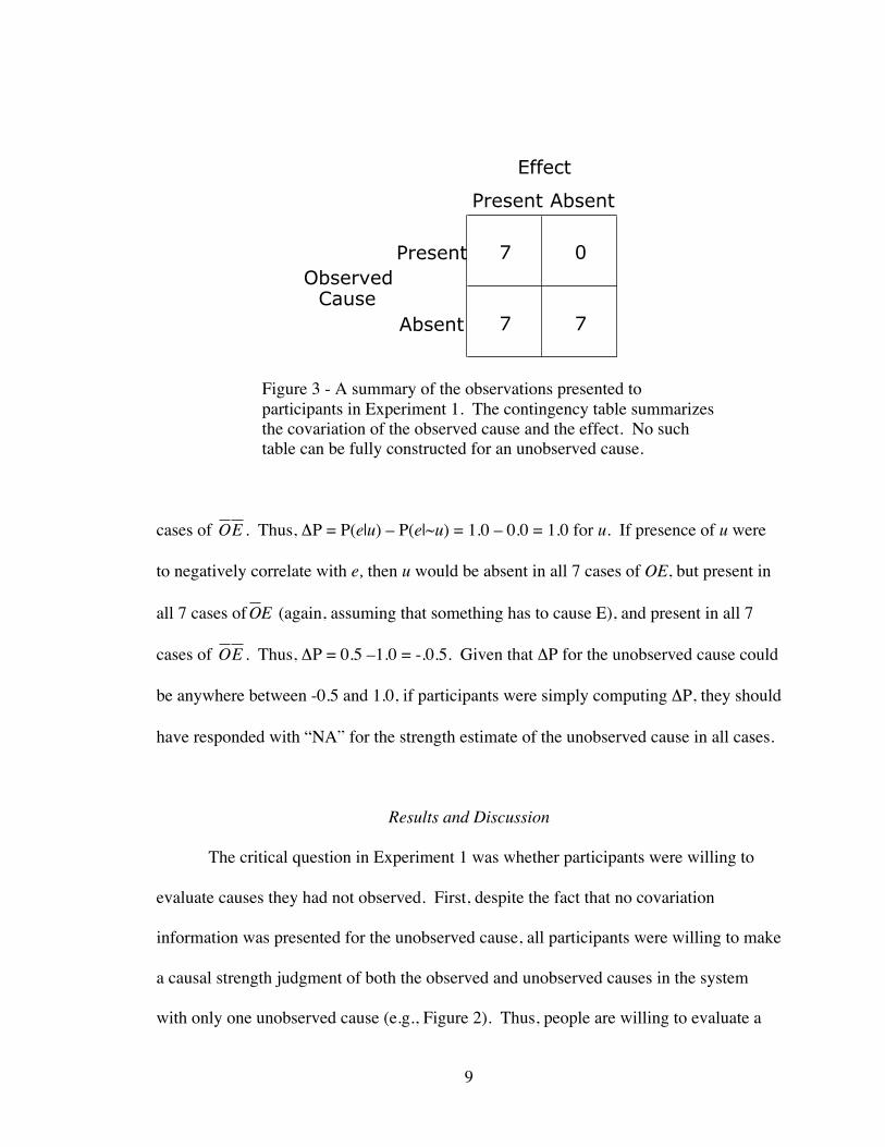
Figure 2 - A sample trial. The states of the grey buttonand the light are observed on every trial. The whitebutton is unobserved; information about its state isunavailable on every trial.

7

they would be examining a series of electrical systems previously constructed by the

experimenters. Participants were told that it was their job to discover how each system

worked and that, to do so, they would view a series of tests that had been run on the

systems. Each of these tests contained information about whether the observed button

was pressed or not and whether or not the light had turned on. Each participant saw all

three systems in a counterbalanced order.

When participants encountered each system they were first told about its

constituent parts (e.g., “One red button, one blue button, and a light.”). Participants were

not told whether this was an exhaustive list of components. They were then told that the

experimenters had run a set of tests on the system to discover how it worked. They were

told that the data pertaining to some of the buttons had been lost so that information about

only a single button and the light would be available on each trial. Participants were also

told that they would be asked to evaluate the extent to which each of two buttons caused

the light to turn on. Which buttons they were to evaluate was indicated in the

instructions. One of the evaluated buttons was always the observed button and the other

was one of the unobserved buttons.

After receiving these instructions, participants proceeded to view the set of tests

(i.e. trials), presented in a randomized order. Trials were presented one at a time and

each remained on the screen until the participant pressed the spacebar to continue.

Participants were then asked to rate the causal strength of two buttons. Each button was

evaluated separately and the observed cause was always evaluated first1. Participants

1 The fixed order of questions provides a strong test of people’s willingness to judgeunobserved causes because judging the observed cause should highlight the lack ofinformation about the unobserved cause.

8

were asked to judge, “the extent to which pressing the [color] button caused the light to

turn on.” Participants responded on a scale from –100 ([color] button prevented the light

from turning on) to 100 ([color] button caused the light to turn on), with zero labeled as,

“[color] button had no influence on the light.”

To estimate participants’ willingness to respond to these questions, participants

were instructed to respond with “N/A” when they felt they could not make a judgment.

Below the rating scale was a reminder that, “If you cannot make a judgment, please write

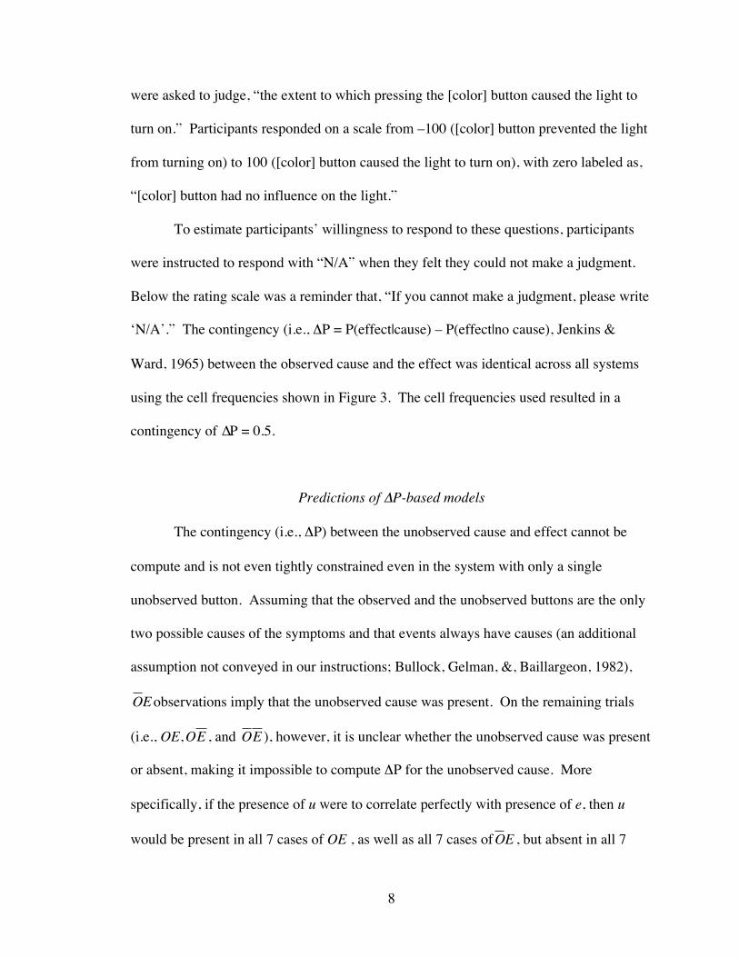
‘N/A’.” The contingency (i.e., ΔP = P(effect|cause) – P(effect|no cause), Jenkins &

Ward, 1965) between the observed cause and the effect was identical across all systems

using the cell frequencies shown in Figure 3. The cell frequencies used resulted in a

contingency of ∆P = 0.5.

Predictions of ΔP-based models

The contingency (i.e., ΔP) between the unobserved cause and effect cannot be

compute and is not even tightly constrained even in the system with only a single

unobserved button. Assuming that the observed and the unobserved buttons are the only

two possible causes of the symptoms and that events always have causes (an additional

assumption not conveyed in our instructions; Bullock, Gelman, &, Baillargeon, 1982),

€

OEobservations imply that the unobserved cause was present. On the remaining trials

(i.e., OE,

€

OE , and

€

OE ), however, it is unclear whether the unobserved cause was present

or absent, making it impossible to compute ΔP for the unobserved cause. More

specifically, if the presence of u were to correlate perfectly with presence of e, then u

would be present in all 7 cases of OE , as well as all 7 cases of

€

OE , but absent in all 7

9

cases of

€

OE . Thus, ΔP = P(e|u) – P(e|~u) = 1.0 – 0.0 = 1.0 for u. If presence of u were

to negatively correlate with e, then u would be absent in all 7 cases of OE, but present in

all 7 cases of

€

OE (again, assuming that something has to cause E), and present in all 7

cases of

€

OE . Thus, ΔP = 0.5 –1.0 = -.0.5. Given that ΔP for the unobserved cause could

be anywhere between -0.5 and 1.0, if participants were simply computing ΔP, they should

have responded with “NA” for the strength estimate of the unobserved cause in all cases.

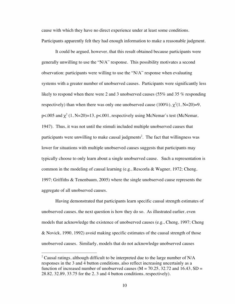
Results and Discussion

The critical question in Experiment 1 was whether participants were willing to

evaluate causes they had not observed. First, despite the fact that no covariation

information was presented for the unobserved cause, all participants were willing to make

a causal strength judgment of both the observed and unobserved causes in the system

with only one unobserved cause (e.g., Figure 2). Thus, people are willing to evaluate a

Present Absent

Present 7 0

Absent 7 7

Effect

ObservedCause

Figure 3 - A summary of the observations presented toparticipants in Experiment 1. The contingency table summarizesthe covariation of the observed cause and the effect. No suchtable can be fully constructed for an unobserved cause.

10

cause with which they have no direct experience under at least some conditions.

Participants apparently felt they had enough information to make a reasonable judgment.

It could be argued, however, that this result obtained because participants were

generally unwilling to use the “N/A” response. This possibility motivates a second

observation: participants were willing to use the “N/A” response when evaluating

systems with a greater number of unobserved causes. Participants were significantly less

likely to respond when there were 2 and 3 unobserved causes (55% and 35 % responding

respectively) than when there was only one unobserved cause (100%), χ2(1, N=20)=9,

p<.005 and χ2 (1, N=20)=13, p<.001, respectively using McNemar’s test (McNemar,

1947). Thus, it was not until the stimuli included multiple unobserved causes that

participants were unwilling to make causal judgments2. The fact that willingness was

lower for situations with multiple unobserved causes suggests that participants may

typically choose to only learn about a single unobserved cause. Such a representation is

common in the modeling of causal learning (e.g., Rescorla & Wagner, 1972; Cheng,

1997; Griffiths & Tenenbaum, 2005) where the single unobserved cause represents the

aggregate of all unobserved causes.

Having demonstrated that participants learn specific causal strength estimates of

unobserved causes, the next question is how they do so. As illustrated earlier, even

models that acknowledge the existence of unobserved causes (e.g., Cheng, 1997; Cheng

& Novick, 1990, 1992) avoid making specific estimates of the causal strength of those

unobserved causes. Similarly, models that do not acknowledge unobserved causes

2 Causal ratings, although difficult to be interpreted due to the large number of N/Aresponses in the 3 and 4 button conditions, also reflect increasing uncertainly as afunction of increased number of unobserved causes (M = 70.25, 32.72 and 16.43, SD =28.82, 32.89, 33.75 for the 2, 3 and 4 button conditions, respectively).

11

(White, 2002; Schustack & Sternberg, 1981; Jenkins & Ward, 1965) cannot make causal

strength judgments about unobserved causes because covariation is unavailable. In what

follows, we describe causal learning models that can handle unobserved cause learning.

In Part 2, we present BUCKLE’s account. In Part 3, we present alternative, existing

accounts (Rescorla & Wagner, 1972; Thagard, 2000)3.

3 Griffiths and Tenenbaum’s (2005) causal support model will not be discussed in thispaper because it concerns the learning of causal structure and not causal strength, whichis the main question of this paper.

12

CHAPTER III

BUCKLE

To learn about causal relationships, BUCKLE uses two steps, each of which is

performed during each observation. The first step is to replace the missing information

about unobserved causes. BUCKLE computes the probability that the unobserved cause

is present based on the available information and the known roles of causes and effects.

Once this step is completed, the unobserved cause is treated just like an observed cause; it

is present with some probability. The second step is to learn the strengths of each cause-

effect relationship. This learning is accomplished via an error-correction algorithm.

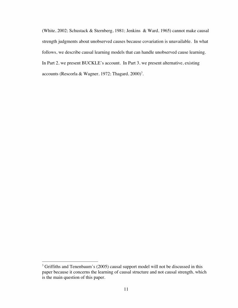
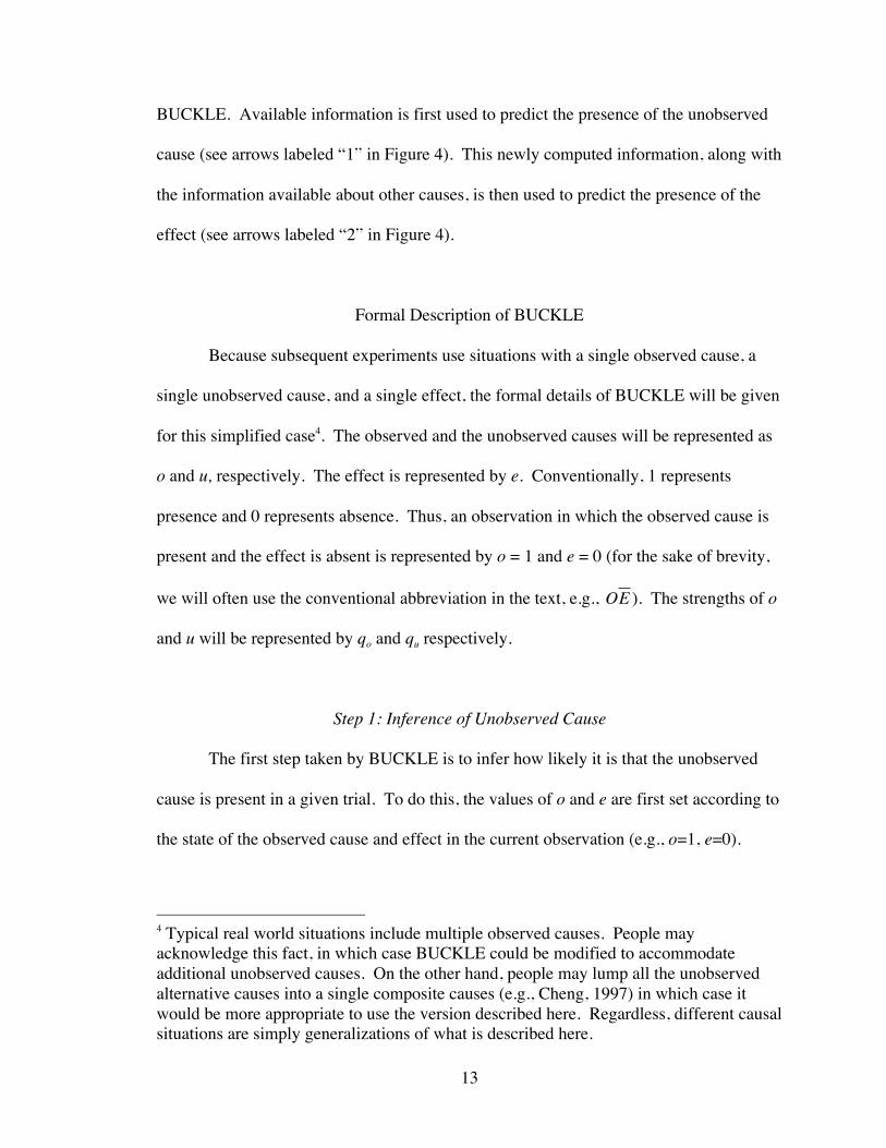
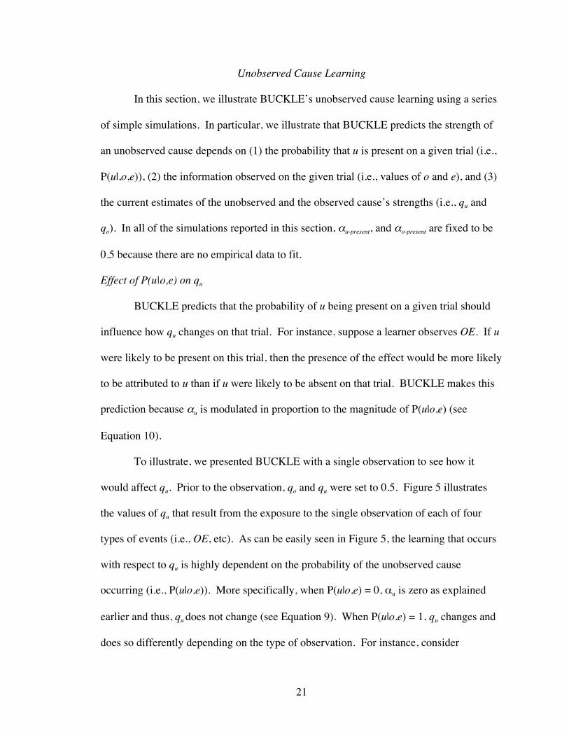
The bi-directionality of these two steps (illustrated in Figure 4) is the essence of

Figure 4 - A diagram illustrating the operation of BUCKLE’s two steps. Thesolid arrows labeled with a “1” represent BUCKLE’s first step: availableinformation about the state of the observed cause and effect is used to predict thelikelihood of the unobserved cause. The dashed arrows labeled with a “2”represent BUCKLE’s second step: information about the two causes is used topredict the effect.

Unobserved Cause

Observed Cause

Effect1 1

2

2

13

BUCKLE. Available information is first used to predict the presence of the unobserved

cause (see arrows labeled “1” in Figure 4). This newly computed information, along with

the information available about other causes, is then used to predict the presence of the

effect (see arrows labeled “2” in Figure 4).

Formal Description of BUCKLE

Because subsequent experiments use situations with a single observed cause, a

single unobserved cause, and a single effect, the formal details of BUCKLE will be given

for this simplified case4. The observed and the unobserved causes will be represented as

o and u, respectively. The effect is represented by e. Conventionally, 1 represents

presence and 0 represents absence. Thus, an observation in which the observed cause is

present and the effect is absent is represented by o = 1 and e = 0 (for the sake of brevity,

we will often use the conventional abbreviation in the text, e.g.,

€

OE ). The strengths of o

and u will be represented by qo and qu respectively.

Step 1: Inference of Unobserved Cause

The first step taken by BUCKLE is to infer how likely it is that the unobserved

cause is present in a given trial. To do this, the values of o and e are first set according to

the state of the observed cause and effect in the current observation (e.g., o=1, e=0).

4 Typical real world situations include multiple observed causes. People mayacknowledge this fact, in which case BUCKLE could be modified to accommodateadditional unobserved causes. On the other hand, people may lump all the unobservedalternative causes into a single composite causes (e.g., Cheng, 1997) in which case itwould be more appropriate to use the version described here. Regardless, different causalsituations are simply generalizations of what is described here.

14

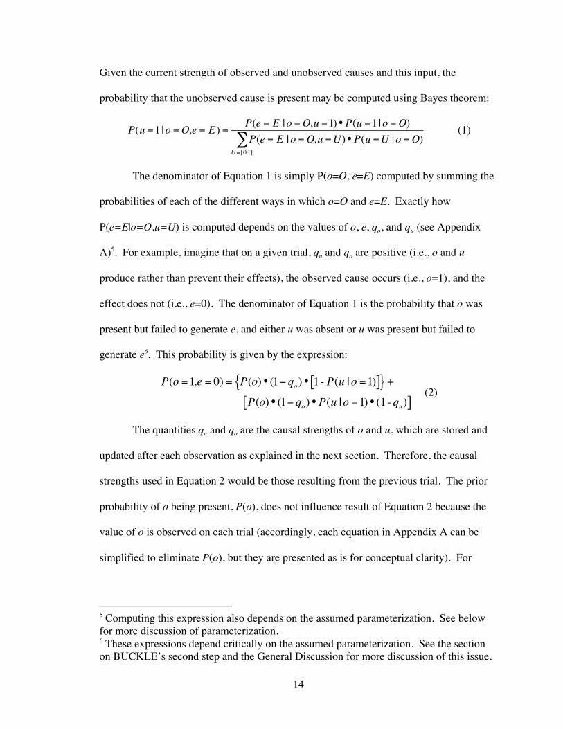
Given the current strength of observed and unobserved causes and this input, the

probability that the unobserved cause is present may be computed using Bayes theorem:

€

P(u =1 |o =O,e = E) =P(e = E |o =O,u =1)•P(u =1 |o =O)P(e = E |o =O,u =U)•P(u =U |o =O)

U=[0,1]∑

(1)

The denominator of Equation 1 is simply P(o=O, e=E) computed by summing the

probabilities of each of the different ways in which o=O and e=E. Exactly how

P(e=E|o=O,u=U) is computed depends on the values of o, e, qo, and qu (see Appendix

A)5. For example, imagine that on a given trial, qu and qo are positive (i.e., o and u

produce rather than prevent their effects), the observed cause occurs (i.e., o=1), and the

effect does not (i.e., e=0). The denominator of Equation 1 is the probability that o was

present but failed to generate e, and either u was absent or u was present but failed to

generate e6. This probability is given by the expression:

€

P(o =1,e = 0) = P(o)• (1− qo)• 1- P(u |o =1)[ ]{ } +P(o)• (1− qo)•P(u |o =1)• (1- qu)[ ]

(2)

The quantities qu and qo are the causal strengths of o and u, which are stored and

updated after each observation as explained in the next section. Therefore, the causal

strengths used in Equation 2 would be those resulting from the previous trial. The prior

probability of o being present, P(o), does not influence result of Equation 2 because the

value of o is observed on each trial (accordingly, each equation in Appendix A can be

simplified to eliminate P(o), but they are presented as is for conceptual clarity). For

5 Computing this expression also depends on the assumed parameterization. See belowfor more discussion of parameterization.6 These expressions depend critically on the assumed parameterization. See the sectionon BUCKLE’s second step and the General Discussion for more discussion of this issue.

15

P(u|o), we will use a uniform distribution (P(u|o=1)= P(u|o=0)= .5) and that remains

static.

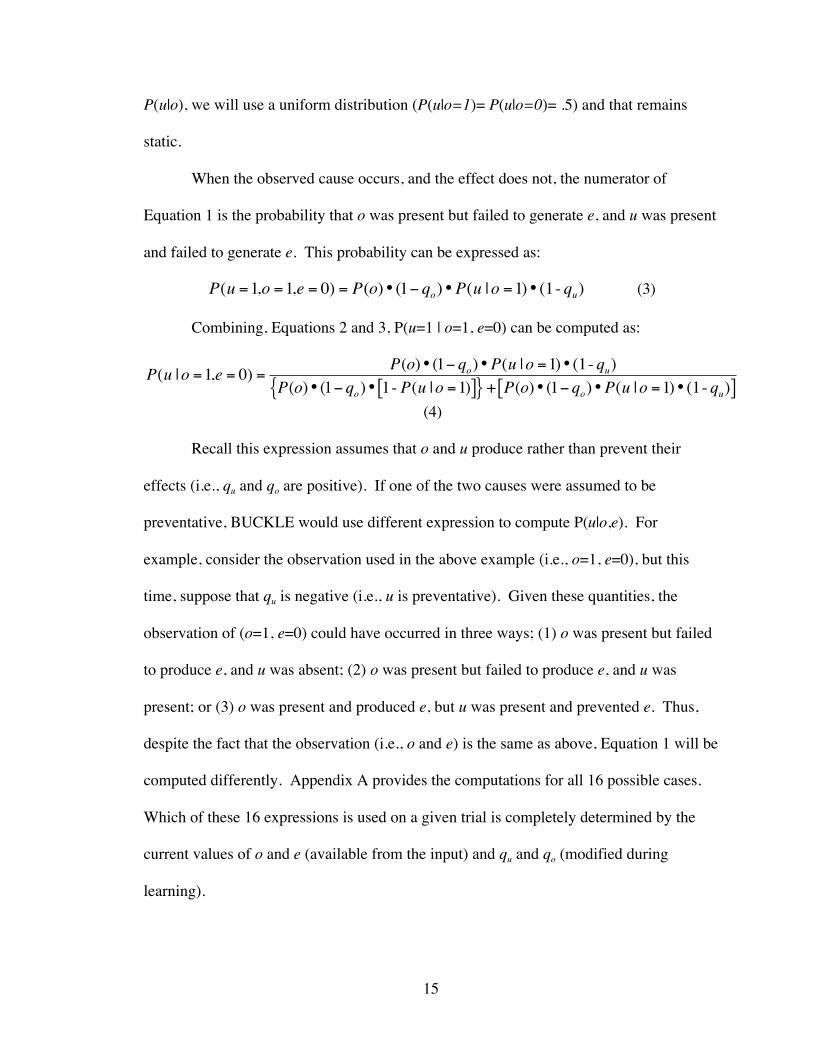
When the observed cause occurs, and the effect does not, the numerator of

Equation 1 is the probability that o was present but failed to generate e, and u was present

and failed to generate e. This probability can be expressed as:

€

P(u =1,o =1,e = 0) = P(o)• (1− qo)•P(u |o =1)• (1- qu) (3)

Combining, Equations 2 and 3, P(u=1 | o=1, e=0) can be computed as:

€

P(u |o =1,e = 0) =P(o)• (1− qo)•P(u |o =1)• (1- qu)

P(o)• (1− qo)• 1- P(u |o =1)[ ]{ } + P(o)• (1− qo)•P(u |o =1)• (1- qu)[ ] (4)

Recall this expression assumes that o and u produce rather than prevent their

effects (i.e., qu and qo are positive). If one of the two causes were assumed to be

preventative, BUCKLE would use different expression to compute P(u|o,e). For

example, consider the observation used in the above example (i.e., o=1, e=0), but this

time, suppose that qu is negative (i.e., u is preventative). Given these quantities, the

observation of (o=1, e=0) could have occurred in three ways; (1) o was present but failed

to produce e, and u was absent; (2) o was present but failed to produce e, and u was

present; or (3) o was present and produced e, but u was present and prevented e. Thus,

despite the fact that the observation (i.e., o and e) is the same as above, Equation 1 will be

computed differently. Appendix A provides the computations for all 16 possible cases.

Which of these 16 expressions is used on a given trial is completely determined by the

current values of o and e (available from the input) and qu and qo (modified during

learning).

16

Step 2: Learning Algorithm

The second step of BUCKLE is to use the available (observed and inferred)

information to learn about the strength of each causal relationship. The algorithm

BUCKLE uses to learn is adapted from a suggestion by Danks, et al. (2003; see the

section titled Similarity between BUCKLE and Other Models of Learning in the General

Discussion)7. This learning algorithm relies on error-correction to learn causal

relationships. Information about the presence (i.e., o and e) is first used to predict how

likely the effect is to be present given the current set of beliefs (i.e., qo and qo). This

prediction is then compared with whether or not the effect actually occurred. The

difference between the predicted and actual states of the effect (the error) forms the basis

of learning.

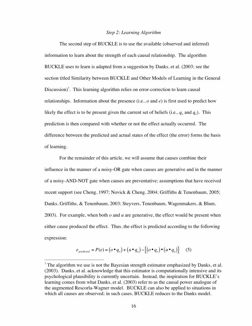
For the remainder of this article, we will assume that causes combine their

influence in the manner of a noisy-OR gate when causes are generative and in the manner

of a noisy-AND-NOT gate when causes are preventative; assumptions that have received

recent support (see Cheng, 1997; Novick & Cheng, 2004; Griffiths & Tenenbaum, 2005;

Danks, Griffiths, & Tenenbaum, 2003; Steyvers, Tenenbaum, Wagenmakers, & Blum,

2003). For example, when both o and u are generative, the effect would be present when

either cause produced the effect. Thus, the effect is predicted according to the following

expression:

€

epredicted = P(e) = o•qo( ) + u•qu( ) − o•qo( ) • u•qu( )[ ] (5)

7 The algorithm we use is not the Bayesian strength estimator emphasized by Danks, et al.(2003). Danks, et al. acknowledge that this estimator is computationally intensive and itspsychological plausibility is currently uncertain. Instead, the inspiration for BUCKLE’slearning comes from what Danks, et al. (2003) refer to as the causal power analogue ofthe augmented Rescorla-Wagner model. BUCKLE can also be applied to situations inwhich all causes are observed; in such cases, BUCKLE reduces to the Danks model.

17

In this expression, o is equal to one when the observed cause is present and zero

when absent, and u is the probability that the unobserved cause is present on this trial

(i.e., P(u|o,e)). When u is preventative and o is generative (i.e. qu < 0, qo > 0), e is

predicted according to the following:

€

epredicted = P(e) = o•qo • u• 1− (−qu)( )[ ] + 1− u[ ]{ } (6)

When u is generative and o is preventative (i.e. qu > 0, qo < 0), e is predicted

according to the following:

€

epredicted = P(e) = u•qu • o• 1− (−qo)( )[ ] + 1− o[ ]{ } (7)

When neither cause is generative, P(e)=0. These are the equations that BUCKLE

uses to make its predictions. The resulting quantity, epredicted, is used as the predicted value

of e. The difference between epredicted and the actual value of e is used to adjust causal

strengths according to the following expressions:

€

qo(n ) = qo(n−1) +αoβ(e − epredicted ) (8)

€

qu(n ) = qu(n−1) +αuβ(e − epredicted ) (9)

The quantities

€

qo(n−1) and

€

qo(n−1) are the causal strengths resulting from the

preceding trial. The strength of each cause is updated separately. The quantities α and β

represent learning rates associated with causes and effects, respectively. A value of 0.5 is

used for β. When the observed cause is present, αo=αo-present where αo-present will be treated

as a free parameter and allowed to vary between zero and one. When the observed cause

is absent, αo=αabsent=0.0. For the unobserved cause, Equation 10 is used to compute a

value of α to take into account the fact that the unobserved cause is only present with

some probability.

18

€

αu = P(u |o,e)• (αu− present −αabsent )[ ] +αabsent (10)

This equation results in αu=0 when P(u|,o,e)=0, and αu=αu-present when P(u|,o,e)=1, just as

for the observed cause. For values of P(u|,o,e) between 0 and 1, α increases linearly and

in proportion to the value of P(u|,o,e). The variable αu-present will be treated as a second

free parameter and allowed to vary between zero and one.

To review, BUCKLE completes two steps for each observation. BUCKLE first

infers how likely the unobserved cause is to be present and then learns the causal

strengths of all causes. Beyond these two steps, the particular algorithms behind each

step of BUCKLE’s operation are interchangeable (see the section entitled The

Interchangeable Nature of BUCKLE in the General Discussion for more discussion on

this point).

Simulation of BUCKLE

In this section, we illustrate BUCKLE’s behavior using a series of simulations.

The first order of business is to ensure that BUCKLE can replicate people’s judgments of

observed causes in a traditional causal learning paradigm. After doing so, we begin

evaluating BUCKLE’s learning of unobserved causes.

Observed Cause Learning

To illustrate BUCKLE’s ability to account learning in a traditional paradigm, we

simulate the results from Experiment 3 of Buehner, Clifford, & Cheng (2003). This

experiment was chosen for three reasons. First, BUCKLE computes the sufficiency of a

cause (i.e., the probability that an effect would occur given that a cause is present), and

19

Buehner et al. (2003) is one of the few existing studies that judiciously asked participants

to judge the sufficiency of a cause (see Buehner, Clifford, & Cheng, 2003 for a

discussion about causal questions). Second, BUCKLE, in its current form, can only learn

from trial-by-trial presentation (as opposed to a summary format where the contingency

information is conveyed all at once) because it updates its beliefs as each trial is

presented. Buehner et al.’s (2003) Experiment 3 utilized this presentation format. Third,

this dataset provides a range of findings and allows us to evaluate BUCKLE’s generality.

In an attempt to provide a thorough test of the Power PC theory (Cheng, 1997), Buehner,

et al. designed ten different conditions, each of which contained a different set of

covariation information. These conditions implied causal strengths (according to the

Power PC theory) ranging from –1 to 1 and included a range of generative, preventative,

and non-contingent conditions.

In Buehner et al.’s Experiment 3, participants received each of the 10 conditions

separately with the observations (24 of them per condition) presented in a random order.

On each trial, information about whether or not a new patient had taken medication was

presented on the computer screen. After one second, information about whether or not

the patient had a headache was presented alongside the cause information. After all the

trials for a condition were presented, participants were asked to judge the strength of the

medication-headache relationship.

To determine whether BUCKLE is able to capture the basic features of people’s

learning, we ran BUCKLE in each of the ten conditions from Experiment 3 of Buehner,

et al. (2003). Since BUCKLE is sensitive to trial order (see Experiment 7) it is important

to simulate the experiment using the identical presentation order. However, Buehner, et

20

al. (2003) used randomized orders for each participant and did not report these orders.

For this reason, we created 1000 simulated participants (i.e., 1000 new presentation

orders). For each simulated participant, the order of the observations in each condition

was randomized (just as in Buehner, et al., 2003). Using the directed search algorithm

described by Hooke and Jeeves (1960), BUCKLE’s αo-present and αu-present were fit to the

mean causal judgments reported by Buehner, et al. This was done for each simulated

participant. All other parameters were set as described in Table A1. The final values of

the strength parameter qo (multiplied by 100 to match the scale used by participants) were

taken as the judged strength of the cause. (In all subsequent simulations of BUCKLE, the

methods described here will be used unless noted otherwise.)

To assess BUCKLE’s fit, we computed both R2 and the root-mean-squared

deviation (RMSD = SQRT(SSE/(N)), where N is the number of observations modeled, or

conditions in this case, 10; Shunn & Wallach, 2002). BUCKLE accounted for 98% of the

variance in participants’ judgments and resulted in an RMSD of 14.45. This fit appears

to be as good as the Power PC theory itself (R2=.97 and RMSD=24.00) and better than

ΔP (R2=.87 and RMSD=18.62). Of course, because these models differ in the number of

free parameters (Power PC and ΔP are parameter-free), it is difficult to assess relative

goodness of fit. (Experiment 6 also addresses the Power PC theory’s predictions about

observed cause learning.) The point of the current simulation, although not diagnostic in

distinguishing between these models, is that BUCKLE is able to account for a significant

portion of people’s behavior in traditional causal learning situations (i.e., those that do

not involve obvious unobserved causes).

21

Unobserved Cause Learning

In this section, we illustrate BUCKLE’s unobserved cause learning using a series

of simple simulations. In particular, we illustrate that BUCKLE predicts the strength of

an unobserved cause depends on (1) the probability that u is present on a given trial (i.e.,

P(u|,o,e)), (2) the information observed on the given trial (i.e., values of o and e), and (3)

the current estimates of the unobserved and the observed cause’s strengths (i.e., qu and

qo). In all of the simulations reported in this section, αu-present, and αo-present are fixed to be

0.5 because there are no empirical data to fit.

Effect of P(u|o,e) on qu

BUCKLE predicts that the probability of u being present on a given trial should

influence how qu changes on that trial. For instance, suppose a learner observes OE. If u

were likely to be present on this trial, then the presence of the effect would be more likely

to be attributed to u than if u were likely to be absent on that trial. BUCKLE makes this

prediction because αu is modulated in proportion to the magnitude of P(u|o,e) (see

Equation 10).

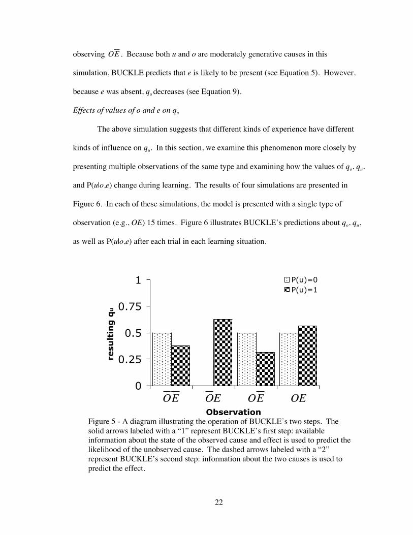
To illustrate, we presented BUCKLE with a single observation to see how it

would affect qu. Prior to the observation, qo and qu were set to 0.5. Figure 5 illustrates

the values of qu that result from the exposure to the single observation of each of four

types of events (i.e., OE, etc). As can be easily seen in Figure 5, the learning that occurs

with respect to qu is highly dependent on the probability of the unobserved cause

occurring (i.e., P(u|o,e)). More specifically, when P(u|o,e) = 0, αu is zero as explained

earlier and thus, qu does not change (see Equation 9). When P(u|o,e) = 1, qu changes and

does so differently depending on the type of observation. For instance, consider

22

observing

€

OE . Because both u and o are moderately generative causes in this

simulation, BUCKLE predicts that e is likely to be present (see Equation 5). However,

because e was absent, qu decreases (see Equation 9).

Effects of values of o and e on qu

The above simulation suggests that different kinds of experience have different

kinds of influence on qu. In this section, we examine this phenomenon more closely by

presenting multiple observations of the same type and examining how the values of qo, qu,

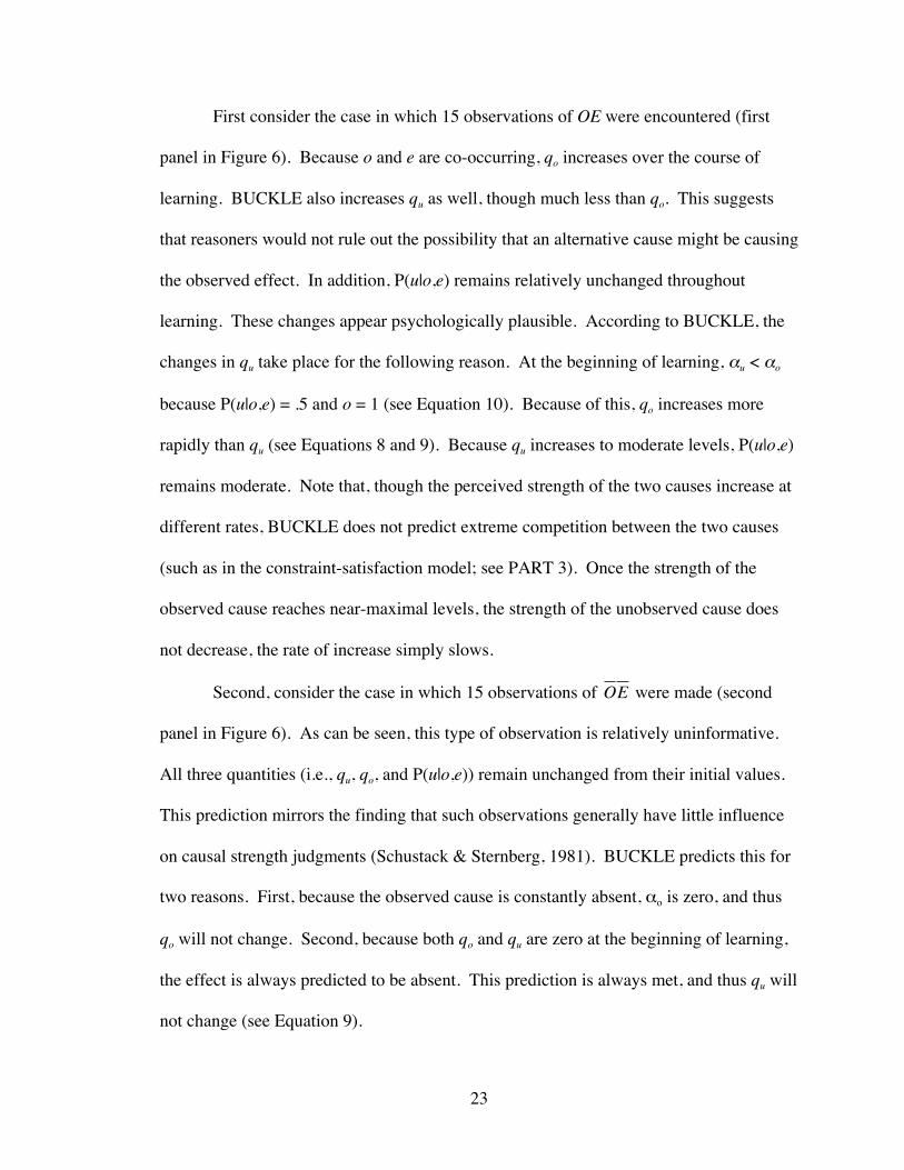
and P(u|o,e) change during learning. The results of four simulations are presented in

Figure 6. In each of these simulations, the model is presented with a single type of

observation (e.g., OE) 15 times. Figure 6 illustrates BUCKLE’s predictions about qo, qu,

as well as P(u|o,e) after each trial in each learning situation.

Figure 5 - A diagram illustrating the operation of BUCKLE’s two steps. Thesolid arrows labeled with a “1” represent BUCKLE’s first step: availableinformation about the state of the observed cause and effect is used to predict thelikelihood of the unobserved cause. The dashed arrows labeled with a “2”represent BUCKLE’s second step: information about the two causes is used topredict the effect.

0

0.25

0.5

0.75

1

Observation

resu

ltin

g q

u

P(u)=0P(u)=1

€

OE

€

OE

€

OE

€

OE

23

First consider the case in which 15 observations of OE were encountered (first

panel in Figure 6). Because o and e are co-occurring, qo increases over the course of

learning. BUCKLE also increases qu as well, though much less than qo. This suggests

that reasoners would not rule out the possibility that an alternative cause might be causing

the observed effect. In addition, P(u|o,e) remains relatively unchanged throughout

learning. These changes appear psychologically plausible. According to BUCKLE, the

changes in qu take place for the following reason. At the beginning of learning, αu < αo

because P(u|o,e) = .5 and o = 1 (see Equation 10). Because of this, qo increases more

rapidly than qu (see Equations 8 and 9). Because qu increases to moderate levels, P(u|o,e)

remains moderate. Note that, though the perceived strength of the two causes increase at

different rates, BUCKLE does not predict extreme competition between the two causes

(such as in the constraint-satisfaction model; see PART 3). Once the strength of the

observed cause reaches near-maximal levels, the strength of the unobserved cause does

not decrease, the rate of increase simply slows.

Second, consider the case in which 15 observations of

€

OE were made (second

panel in Figure 6). As can be seen, this type of observation is relatively uninformative.

All three quantities (i.e., qu, qo, and P(u|o,e)) remain unchanged from their initial values.

This prediction mirrors the finding that such observations generally have little influence

on causal strength judgments (Schustack & Sternberg, 1981). BUCKLE predicts this for

two reasons. First, because the observed cause is constantly absent, αo is zero, and thus

qo will not change. Second, because both qo and qu are zero at the beginning of learning,

the effect is always predicted to be absent. This prediction is always met, and thus qu will

not change (see Equation 9).

24

0

0.5

1

0 1 2 3 4 5 6 7 8 9 10 11 12 13 14 15Trial Number

Cau

sal S

tren

gth

0

0.5

1

P(u

)

P(u)

quqo

0

0.5

1

0 1 2 3 4 5 6 7 8 9 10 11 12 13 14 15

Trial Number

Cau

sal S

tren

gth

0

0.5

1P

(u)

P(u)qo

qu

0

0.5

1

0 1 2 3 4 5 6 7 8 9 10 11 12 13 14 15Trial Number

Cau

sal S

tren

gth

0

0.5

1

P(u

)P(u)qo

qu

0

0.5

1

0 1 2 3 4 5 6 7 8 9 10 11 12 13 14 15Trial Number

Cau

sal S

tren

gth

0

0.5

1

P(u

)

P(u)

quqo

Figure 6 - BUCKLE’s predictions about how qu, qo, and P(u|,o,e) will changeover time in four situations. In each case, a single type of observation (e.g.,

€

OE ) was presented for 15 trials.

25

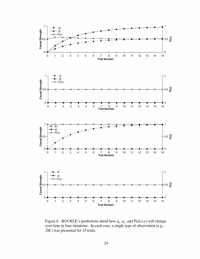
Third, consider the case in which 15 observations of

€

OE were made (third panel

in Figure 6). In this case, qo remains 0, but qu increases. This is because

€

OE necessarily

implicates the operation of an unobserved cause (Luhmann & Ahn, 2003). Because the

observed cause is absent, it could not have generated the effect. The only way in which

an

€

OE observation could have occurred is if an unobserved cause was present and

generated the effect. This is reflected in the probability computation found in Appendix

A. That is, assuming that qu >=0 (i.e., assuming u is not preventative), when o=0 and

e=1, the probability of u is always 1. The certainty with which the unobserved cause is

present allows αu to reach maximal levels (see Equation 10) and thus leads to large

changes in qu (see Equation 9); the perceived strength of the unobserved cause increases

significantly. Because of the special status of

€

OE observations, we will often refer to

them by the more meaningful label: unexplained effects (Luhmann & Ahn, 2003).

The significant influence of unexplained effects predicted by BUCKLE is in line

with several previous empirical demonstrations. Luhmann and Ahn (2003) and

Hagmayer and Waldmann (2004) have already demonstrated the influence of

unexplained effects on inferences about unobserved causes (Luhmann and Ahn’s (2003)

experiments are reported in detail later in this paper). For instance, Hagmayer and

Waldmann (2004) varied

€

P(E |O) from zero to .67, and asked participants to estimate

the causal strength of both the observed and unobserved causes. They found that when

€

P(E |O) was high, the unobserved cause was perceived as strong, and when

€

P(E |O)

was low, the unobserved cause was perceived as weak.

Finally, consider the case in which 15 observations of

€

OE are made (bottom

panel in Figure 6). One might expect that

€

OE observations would have a similar effect

26

on the perceived causal strength of unobserved causes as

€

OE ; these observations could

suggest that an unobserved cause prevented the effect from occurring. If this were the

case, then the unobserved cause should be perceived as preventative (i.e., qu<0).

However, as can be seen in Figure 6, this is not the case. Instead, BUCKLE predicts that

€

OE observations have relatively little influence; all three quantities (i.e., qu, qo, and

P(u|,o,e)) again remain unchanged over the course of learning. This is because

€

OE

observations may occur either when the unobserved cause prevents the effect or when the

observed cause is insufficient to bring about the cause (see Equation A11 in Appendix

A). The former interpretation suggests that the unobserved cause is preventative whereas

the latter interpretation allows the unobserved cause to be generative. In the current

simulation, because qo is zero, the former interpretation is more likely. According to

BUCKLE, if the relative probability of the two interpretations were reversed, then

€

OE

observations would lead the unobserved cause to be perceived as preventative.

BUCKLE’s prediction about the influence of

€

OE can be contrasted with the work

of Schulz, Sommerville, and Gopnik (2005). In characterizing the causal learning of

preschoolers, these authors suggest that

€

OE observations necessarily suggest the

influence of (preventative) unobserved causes. Indeed, when

€

OE observations were

encountered in a situation containing an unobserved cause (their Experiment 1), children

who were asked to prevent the effect preferred to utilize the unobserved cause. Schulz et

al. (2005) suggest that the influence of

€

OE results from preschoolers’ strict belief that

effects necessarily follow their causes. Holding such a belief would be analogous to

modifying BUCKLE’s probability computations such that the observed cause could not

have failed to bring about its effect. Once modified, the ambiguity of

€

OE observations is

27

eliminated and

€

OE observations would lead learners to perceive the unobserved cause as

preventative. It is an empirical question whether adults would also hold such strict

beliefs about causal relations (see current Experiments 2-5 and 7).

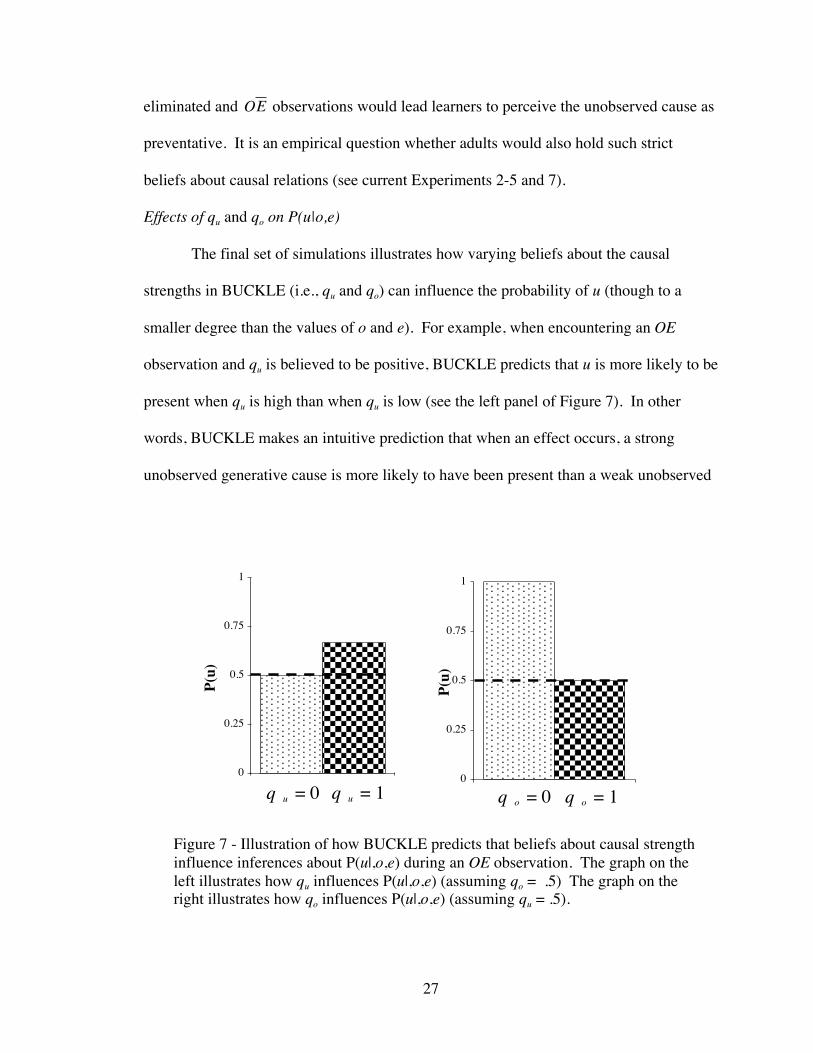
Effects of qu and qo on P(u|o,e)

The final set of simulations illustrates how varying beliefs about the causal

strengths in BUCKLE (i.e., qu and qo) can influence the probability of u (though to a

smaller degree than the values of o and e). For example, when encountering an OE

observation and qu is believed to be positive, BUCKLE predicts that u is more likely to be

present when qu is high than when qu is low (see the left panel of Figure 7). In other

words, BUCKLE makes an intuitive prediction that when an effect occurs, a strong

unobserved generative cause is more likely to have been present than a weak unobserved

Figure 7 - Illustration of how BUCKLE predicts that beliefs about causal strengthinfluence inferences about P(u|,o,e) during an OE observation. The graph on theleft illustrates how qu influences P(u|,o,e) (assuming qo = .5) The graph on theright illustrates how qo influences P(u|,o,e) (assuming qu = .5).

0

0.25

0.5

0.75

1

P(u)

q u = 0 q u = 10

0.25

0.5

0.75

1

P(u)

q o = 0 q o = 1

28

cause is.

Conversely, BUCKLE predicts that when encountering an OE observation, u is

less likely to be present when an observed, generative cause’s strength (qo) is high than

when it is low (see the right panel of Figure 7). In other words, if one believes that an

observed cause is a strong causal candidate, one is less likely to postulate presence of an

unobserved cause than if the observed cause is a weak causal candidate. Both of these

predictions can be derived from Equation A4 in Appendix A.

Summary

BUCKLE learns using two steps. BUCKLE first replaces the missing data using

an assortment of available information. In the second step, BUCKLE learns the causal

relations assuming the unobserved cause is present with some probability. Using a

variety of simple situations, we have illustrated that these steps provide a set of intuitive

predictions.

29

CHAPTER IV

ALTERNATIVE MODELS

We consider two other models that include learning about unobserved causes.

First, we consider constraint-satisfaction models (e.g., Thagard, 2000). These models

suggest that the strength of unobserved causes is inversely related to the strength of an

observed cause, akin to the well-known discounting principle (Kelley, 1967; Morris &

Larrick, 1995). Second, we consider the associative models proposed by Rescorla and

Wagner (1972). This model assumes that unobserved cause is constantly present and

learns about it just as it learns about observed causes. In what follows, we describe each

of these models in more detail and present experiments to compare them.

Constraint-satisfaction Networks

Constraint-satisfaction refers to the process of finding a set of states that satisfies

a set of constraints or criteria and has been studied extensively in the field of artificial

intelligence. In psychology, the states often refer to beliefs and there is evidence that

people engage in constraint-satisfaction both to solve problems (e.g., McClelland &

Rumelhart, 1981) and to remain internally consistent, or coherent (e.g., Holyoak &

Simon, 1999).

In our discussion, we will use one particular variant of constrain-satisfaction

networks: the Interactive Activation and Competition (IAC) model (McClelland &

Rumelhart, 1981). This model has been used to explain a wide variety of psychological

30

findings (Thagard, 2000 for an overview) including aspects of causal learning and

inference (e.g., Read & Marcus-Newhall, 1993; Hagmeyer & Waldmann, 2002). As we

will see, these models also provide an intuitive prediction about how people learn about

unobserved causes.

IAC models are networks in which each node corresponds to either an observation

or explanation. Each node has an activation level that represents the degree to which that

observation or explanation is believed. Positive activation represents belief and negative

activation represents disbelief. Nodes are connected with bi-directional links so that

directly connected nodes have mutual influence on each other. Observation nodes are

connected to explanation nodes with links that either have a positive (consistent) or

negative (inconsistent) weight. Explanations nodes are connected to each other with

negatively weighted links so that explanations are inhibited by active alternative

explanations (Morris & Larrick, 1995; Thagard, 2000; Baker, Mercier, Vallée-

Tourangeau, Frank, & Pan, 1993; Price & Yates, 1993). In addition, observation nodes

are connected to a special node whose activation is always maximal (i.e., 1). This allows

observations (more so than explanations which must be inferred) to be accepted relatively

easily (though it is possible for them to be rejected).

To initiate learning, each node is assigned a small, random amount of activation.

The input to each node, i, is based on the activation of all directly linked nodes, aj, and

the weight of the intervening links, wij.

€

inputi = wij ∗ a jj∑ (11)

31

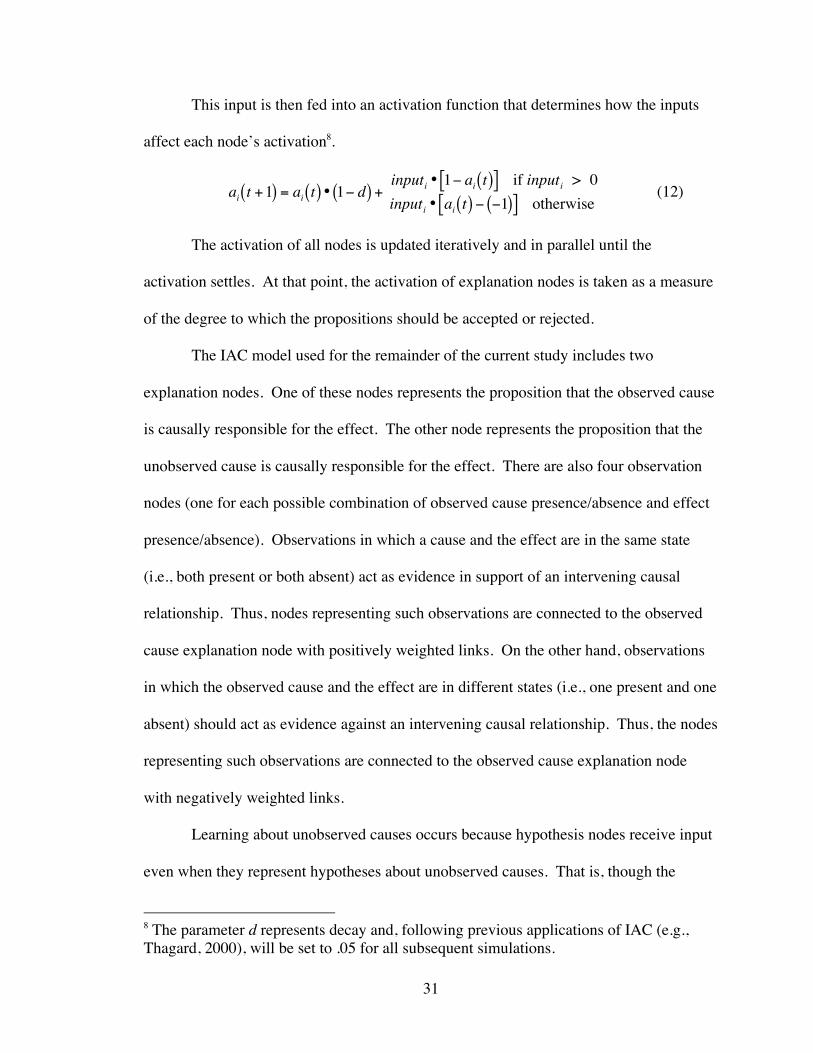
This input is then fed into an activation function that determines how the inputs

affect each node’s activation8.

€

ai t +1( ) = ai t( ) • 1− d( ) +inputi • 1− ai t( )[ ] if inputi > 0inputi • ai t( ) − −1( )[ ] otherwise

(12)

The activation of all nodes is updated iteratively and in parallel until the

activation settles. At that point, the activation of explanation nodes is taken as a measure

of the degree to which the propositions should be accepted or rejected.

The IAC model used for the remainder of the current study includes two

explanation nodes. One of these nodes represents the proposition that the observed cause

is causally responsible for the effect. The other node represents the proposition that the

unobserved cause is causally responsible for the effect. There are also four observation

nodes (one for each possible combination of observed cause presence/absence and effect

presence/absence). Observations in which a cause and the effect are in the same state

(i.e., both present or both absent) act as evidence in support of an intervening causal

relationship. Thus, nodes representing such observations are connected to the observed

cause explanation node with positively weighted links. On the other hand, observations

in which the observed cause and the effect are in different states (i.e., one present and one

absent) should act as evidence against an intervening causal relationship. Thus, the nodes

representing such observations are connected to the observed cause explanation node

with negatively weighted links.

Learning about unobserved causes occurs because hypothesis nodes receive input

even when they represent hypotheses about unobserved causes. That is, though the

8 The parameter d represents decay and, following previous applications of IAC (e.g.,Thagard, 2000), will be set to .05 for all subsequent simulations.

32

unobserved cause explanation receives no input from the observations (because the

information about unobserved cause is unavailable in the input), it does receive input

from the observed cause explanation via the negatively weighted link between them. The

unobserved cause node is thus active to the extent that the competing explanation is

inactive. In turn, a strong unobserved cause will tend to decrease the perceived strength

of the observed cause (similar to the discounting principle). In sum, the constraint-

satisfaction model generally suggests that the perceived strength of an unobserved cause

will be related inversely to the perceived strength of the observed cause.

The Rescorla-Wagner Model

The learning model described by Rescorla and Wagner (1972; RW hereafter)

assigns each cause and effect a node in a simple network. The inputs to the network

represent events that are encountered first (often causes) and the outputs of the network

represent those events that follow (often effects). Each input node is then connected to

each output node. The strength of each cause is represented by the weight of the

connection between its node and the effect node. Causal learning in this model amounts

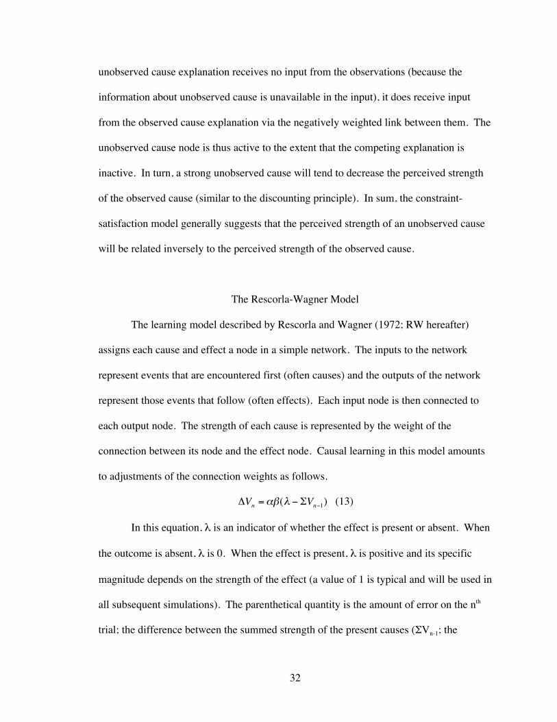
to adjustments of the connection weights as follows.

€

ΔVn =αβ(λ − ΣVn−1) (13)

In this equation, λ is an indicator of whether the effect is present or absent. When

the outcome is absent, λ is 0. When the effect is present, λ is positive and its specific

magnitude depends on the strength of the effect (a value of 1 is typical and will be used in

all subsequent simulations). The parenthetical quantity is the amount of error on the nth

trial; the difference between the summed strength of the present causes (ΣVn-1; the

33

predicted value of the effect) and the observed effect (λ). The saliency of the cause is

represented by α and the saliency of the effect is represented by β.

Thus, according to RW, learning is accomplished via an error-correction

algorithm. The summed causal strength of the present causes acts as a prediction about

the presence of the effect. This prediction is then compared to the actual observation of

the effect. The difference between the prediction and the actual observation is then used

to modify the network weights (i.e. causal strengths). Over time, this algorithm will tend

to minimize the error between the prediction and the observation.

Of particular interest is the fact that RW always learns about an unobserved cause.

Like BUCKLE, RW adds an extra cause node into its network. Unlike BUCKLE, this

cause is assumed to be present on all trials. This unobserved cause is often interpreted as

representing the experimental context or background, but could also be thought of as a

composite of all unobserved causes (e.g., Cheng, 1997). For example, Shanks (1989)

states that, “occurrences of the [effect] in the absence of the target cause … must be

attributed to the background” (p. 27).” Like BUCKLE, RW learns about this unobserved

cause just as it learns about observed causes. Thus, the critical difference between

BUCKLE and RW is that, whereas RW makes a simple assumption about the probability

of the unobserved cause, BUCKLE attempts to make somewhat more sophisticated,

dynamic inferences about the probability of the unobserved cause.

34

CHAPTER V

EMPIRICAL TESTS OF THE MODELS

In what follows, we test these models in 7 experiments. In Experiment 2 the

constraint-satisfaction model is compared with BUCKLE. Recall that the constraint-

satisfaction model predicts an antagonistic relationship between competing explanations

(e.g., causes) whereas BUCKLE does not. Experiment 3 replicates the qualitative

predictions of BUCKLE using more ecologically valid methods. Experiments 4-6

compare RW and BUCKLE. As explained earlier, a critical difference between the two

models is that RW learns about a constantly present unobserved cause, whereas

BUCKLE inferences about the probability of the unobserved cause being present change

over time. In addition, the Power PC theory will be discussed in the context of

Experiment 5. Finally, Experiments 7 and 8 test additional predictions derived from

BUCKLE and attempt to gain a richer understanding of people’s causal learning.

Experiment 2

To test the constraint-satisfaction model, we conducted a causal learning

experiment that varied the statistical relationship between the observed cause and the

effect. The details of simulation results of the two models for this experiment will be

provided later. In this section we simply provide conceptual explanations of the models’

predictions in order to motivate the design of the experiment. The experiment consisted

of four conditions illustrated in Table 1. All four conditions include OE and

€

OE

35

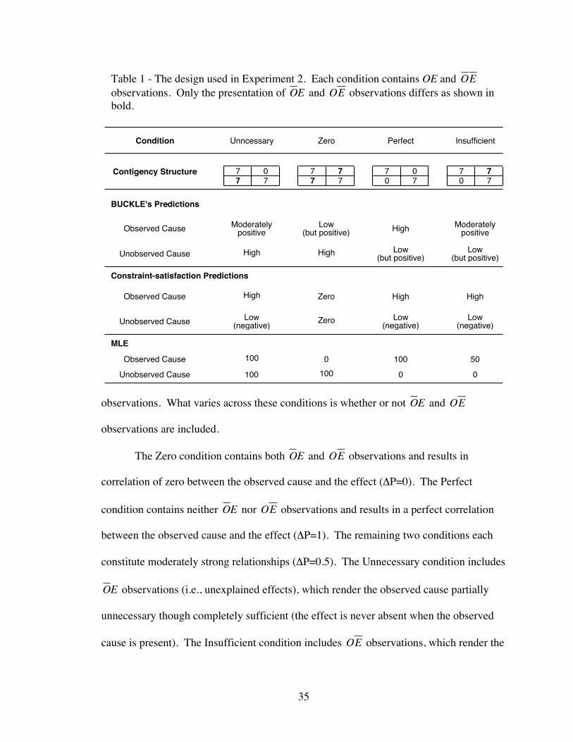
observations. What varies across these conditions is whether or not

€

OE and

€

OE

observations are included.

The Zero condition contains both

€

OE and

€

OE observations and results in

correlation of zero between the observed cause and the effect (ΔP=0). The Perfect

condition contains neither

€

OE nor

€

OE observations and results in a perfect correlation

between the observed cause and the effect (ΔP=1). The remaining two conditions each

constitute moderately strong relationships (ΔP=0.5). The Unnecessary condition includes

€

OE observations (i.e., unexplained effects), which render the observed cause partially

unnecessary though completely sufficient (the effect is never absent when the observed

cause is present). The Insufficient condition includes

€

OE observations, which render the

7 0 7 7 7 0 7 77 7 7 7 0 7 0 7

BUCKLE's Predictions

Observed Cause

Unobserved Cause

Constraint-satisfaction Predictions

Observed Cause

Unobserved Cause

MLE

Observed Cause

Unobserved Cause

Moderately positive

High High Low (but positive)

Low (but positive)

Moderately positive

Low (but positive)

50

100 100 0 0

100 0

Condition

Contigency Structure

Unncessary

100

High

Low (negative)

Low (negative)

High High High

Low (negative)

Zero

Zero

Perfect InsufficientZero

Table 1 - The design used in Experiment 2. Each condition contains OE and

€

OEobservations. Only the presentation of

€

OE and

€

OE observations differs as shown inbold.

36

observed cause partially insufficient though completely necessary (the effect never occurs

in the absence of the observed cause).

Table 1 also contains the predictions of the various models. According to the

constraint-satisfaction model, the unobserved cause should be strongest when the

observed cause is weakest (the Perfect condition). In all other cases, the observed cause

is positively correlated with the effect and thus the unobserved cause should be perceived

as negative. BUCKLE predicts that unexplained effects (i.e.,

€

OE observations) will most

significantly influence unobserved cause judgments. This influence leads BUCKLE to

predict that the unobserved cause should be perceived as stronger in the two conditions

that include unexplained effects (Unnecessary and Zero) than in the two conditions that

do not (Perfect and Insufficient). Thus, the Unnecessary condition provides the most

critical test comparing BUCKLE and the constraint-satisfaction model with respect the

predictions on the unobserved cause.

Those looking for the “correct” causal strengths in these four conditions can look

to the Maximum Likelihood Estimates (MLE) listed in Table 1. These estimates are the

most likely values for qo and qu given an (arguably) reasonable set of assumptions (see

Appendix B for details on how we compute the MLE).

We used two different dependent variables across Experiments 2A and 2B

because different models measure different quantities. BUCKLE estimates causal

sufficiency: the degree to which a cause is sufficient to bring about its effect. The

constraint-satisfaction model computes less specific quantities9. Thus, to test BUCKLE,

9 The constraint-satisfaction model, like RW, measures association (i.e., the degree towhich the cause and effect co-occur). Association, like a regression weight, does not

37

Experiment 2A uses a query that specifically taps the notion of causal sufficiency (see

Buehner, et al., 2003). Experiment 2B uses the traditional, but ambiguous method of

eliciting causal judgments (e.g. To what extent does X cause Y?) typically used when

evaluating constraint-satisfaction models (e.g. Hagmeyer & Waldmann, 2002).

Additionally, participants in Experiments 2A and 2B were told that nothing, other

than the two buttons, could influence the light. This was done to equate participants’

assumptions about the situation with the assumptions used in the modeling reported later.

Experiment 3 will assess people’s more natural assumptions about unobserved causes by

not telling participants about the existence of an unobserved cause until after learning

was completed.

Method

Participants. Fifty-four Vanderbilt University undergraduates (24 in Experiment

2A, 30 in Experiment 2B) participated for partial fulfillment of course credit.

Materials and design. Stimuli consisted of four electrical systems similar to those

used in Experiment 1 (see Figure 2 for an example). Each of the buttons used in the

experiment was a different color to aid in their memory and to ensure that subjects did

not confuse different systems. Each system contained exactly one button whose state

(pressed or not) was observable, one button whose state was unobservable and a single

light. The unavailable state of the unobserved button was denoted via a large question

mark superimposed over the button. The state of the light (on or off) was always

observable.

distinguish between sufficiency and necessity. Association is simply a holistic measureof the strength of a relationship.

38

Both Experiments 2A and 2B used a 2 X 2 factorial design by crossing the

inclusion of

€

OE observations with the inclusion of

€

OE observations. Table 1

summarizes the actual cell frequencies for each condition and the contingency between

the observed cause and the observed effect.

Procedure. The procedure was same as in Experiment 1 except for the following

changes. Each participant saw all four systems in a counterbalanced order. The trials

within each system were presented in a quasi-randomized order. The set of trials was

divided into blocks such that two of each trial type was presented within each block. The

order of trials within these blocks was randomized. This was done to ensure that the

different types of trials were evenly distributed throughout each participant’s experience,

given the previous studies showing the effect of presentation order in causal induction

(e.g., Lopez, Shanks, Almaraz, & Fernandez, 1996; Dennis & Ahn, 2001).

After viewing the entire set of trials, participants were asked to rate the causal

strength of the observed and unobserved button separately. In Experiment 2A,

participants were told to, “Imagine running 100 new tests in which the [color] button was

pressed and the [color] button was not. On how many of these tests do you expect the

light to turn on?” Participants responded with a number between 0 and 100. In

Experiment 2B, participants were asked to, “judge the extent to which pressing the

[color] button caused the light to turn on.” Responses could range from –100 (“[color]

button prevented the light from turning on”) to 100 (“[color] button caused the light to

turn on”) with zero label as, “[color] button had no influence on the light turning on.”

Unlike Experiment 1, participants were not allowed to respond with “N/A.” This

was done for two reasons. First, the willingness to estimate unobserved causes was not

39

the main concern of Experiment 2. Second, although no participant in Experiment 1 gave

“N/A” responses for systems involving an unobserved variable (such as those used in the

current experiment), we wished to maximize the number of numerical responses because

of our primary interest in comparing causal strength estimates across the four conditions.

In addition to the causal strength ratings of the two buttons, participants were also

asked to rate how confident they were in each of their causal judgments. This task was

added in an attempt to disentangle participants’ causal beliefs from confidence in those

beliefs. Doing so also allows us to examine whether participants, although willing to

estimate causal strengths of an unobserved cause, feel as confident about these judgments

as with an observed cause. These confidence ratings were made on a 7-point scale

ranging from 1 (“Not at all confident”) to 7 (“Very confident”). A visual representation

of the scale, indicating the endpoints and their labels, was present for participants’

reference while making their judgments.


Experiment 2A

Participants’ causal judgments can be seen in Figure 8. As predicted by

BUCKLE, the presence of unexplained effects (i.e.,

€

OE ) is particularly influential in

driving judgments of the unobserved cause. A 2 (

€

OE present / absent) X 2 (

€

OE present

/ absent) repeated measures ANOVA on causal judgments of unobserved causes revealed

a significant main effect of unexplained effects (

€

OE observations), F(1, 23) = 43.19, p <

.0001, because participants gave much higher ratings on conditions with unexplained

effects (M = 73.35, SD = 30.27) than on conditions without unexplained effects (M =

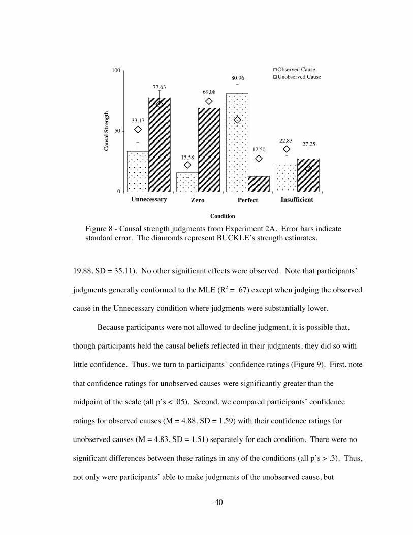
40

19.88, SD = 35.11). No other significant effects were observed. Note that participants’

judgments generally conformed to the MLE (R2 = .67) except when judging the observed

cause in the Unnecessary condition where judgments were substantially lower.

Because participants were not allowed to decline judgment, it is possible that,

though participants held the causal beliefs reflected in their judgments, they did so with

little confidence. Thus, we turn to participants’ confidence ratings (Figure 9). First, note

that confidence ratings for unobserved causes were significantly greater than the

midpoint of the scale (all p’s < .05). Second, we compared participants’ confidence

ratings for observed causes (M = 4.88, SD = 1.59) with their confidence ratings for

unobserved causes (M = 4.83, SD = 1.51) separately for each condition. There were no

significant differences between these ratings in any of the conditions (all p’s > .3). Thus,

not only were participants’ able to make judgments of the unobserved cause, but

Figure 8 - Causal strength judgments from Experiment 2A. Error bars indicatestandard error. The diamonds represent BUCKLE’s strength estimates.

33.17

15.58

80.96

22.83

77.6369.08

12.5027.25

0

50

100

Condition

Cau

sal S

tren

gth

Observed CauseUnobserved Cause

Unnecessary Zero InsufficientPerfect

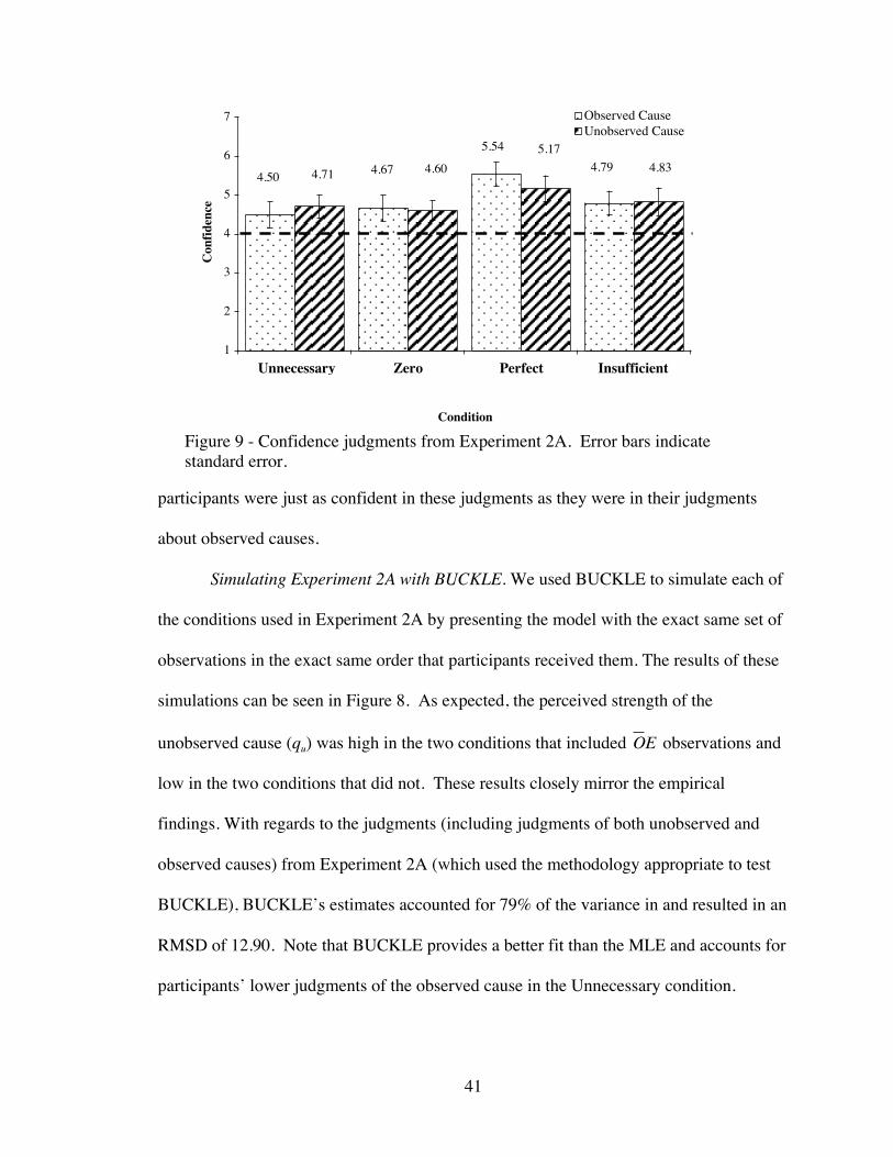
41

participants were just as confident in these judgments as they were in their judgments

about observed causes.

Simulating Experiment 2A with BUCKLE. We used BUCKLE to simulate each of

the conditions used in Experiment 2A by presenting the model with the exact same set of

observations in the exact same order that participants received them. The results of these

simulations can be seen in Figure 8. As expected, the perceived strength of the

unobserved cause (qu) was high in the two conditions that included

€

OE observations and

low in the two conditions that did not. These results closely mirror the empirical

findings. With regards to the judgments (including judgments of both unobserved and

observed causes) from Experiment 2A (which used the methodology appropriate to test

BUCKLE), BUCKLE’s estimates accounted for 79% of the variance in and resulted in an

RMSD of 12.90. Note that BUCKLE provides a better fit than the MLE and accounts for

participants’ lower judgments of the observed cause in the Unnecessary condition.

Figure 9 - Confidence judgments from Experiment 2A. Error bars indicatestandard error.

4.795.54

4.674.504.834.60

5.17

4.71

1

2

3

4

5

6

7

Condition

Confidence


Zero Perfect InsufficientUnnecessary

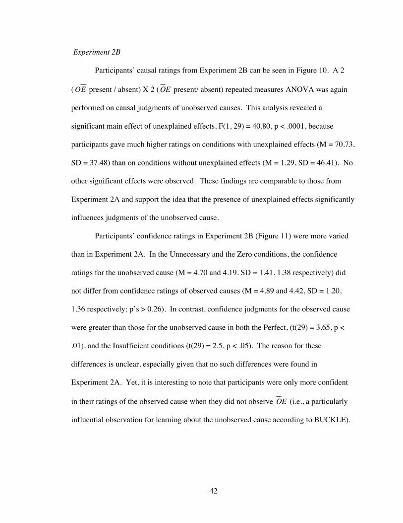
42

Experiment 2B

Participants’ causal ratings from Experiment 2B can be seen in Figure 10. A 2

(

€


€

OE present/ absent) repeated measures ANOVA was again

performed on causal judgments of unobserved causes. This analysis revealed a

significant main effect of unexplained effects, F(1, 29) = 40.80, p < .0001, because

participants gave much higher ratings on conditions with unexplained effects (M = 70.73,

SD = 37.48) than on conditions without unexplained effects (M = 1.29, SD = 46.41). No

other significant effects were observed. These findings are comparable to those from

Experiment 2A and support the idea that the presence of unexplained effects significantly

influences judgments of the unobserved cause.

Participants’ confidence ratings in Experiment 2B (Figure 11) were more varied

than in Experiment 2A. In the Unnecessary and the Zero conditions, the confidence

ratings for the unobserved cause (M = 4.70 and 4.19, SD = 1.41, 1.38 respectively) did

not differ from confidence ratings of observed causes (M = 4.89 and 4.42, SD = 1.20,

1.36 respectively; p’s > 0.26). In contrast, confidence judgments for the observed cause

were greater than those for the unobserved cause in both the Perfect, (t(29) = 3.65, p <

.01), and the Insufficient conditions (t(29) = 2.5, p < .05). The reason for these

differences is unclear, especially given that no such differences were found in

Experiment 2A. Yet, it is interesting to note that participants were only more confident

in their ratings of the observed cause when they did not observe

€

OE (i.e., a particularly

influential observation for learning about the unobserved cause according to BUCKLE).

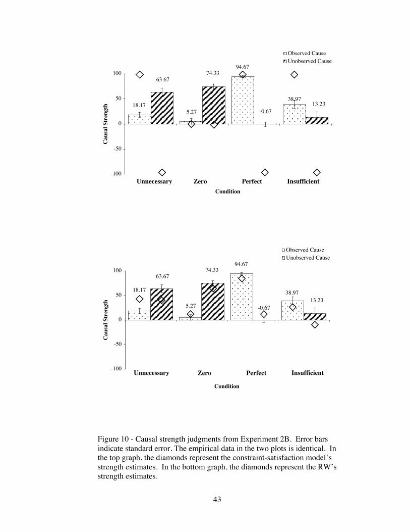
43

Figure 10 - Causal strength judgments from Experiment 2B. Error barsindicate standard error. The empirical data in the two plots is identical. Inthe top graph, the diamonds represent the constraint-satisfaction model’sstrength estimates. In the bottom graph, the diamonds represent the RW’sstrength estimates.

38.97

94.67

5.2718.17 13.23

-0.67

74.3363.67

-100

-50

0

50

100

Condition

Cau

sal S

tren

gth



38.9718.17

5.27

94.67

63.6774.33

-0.6713.23

-100

-50

0

50

100

Condition

Cau

sal S

tren

gth



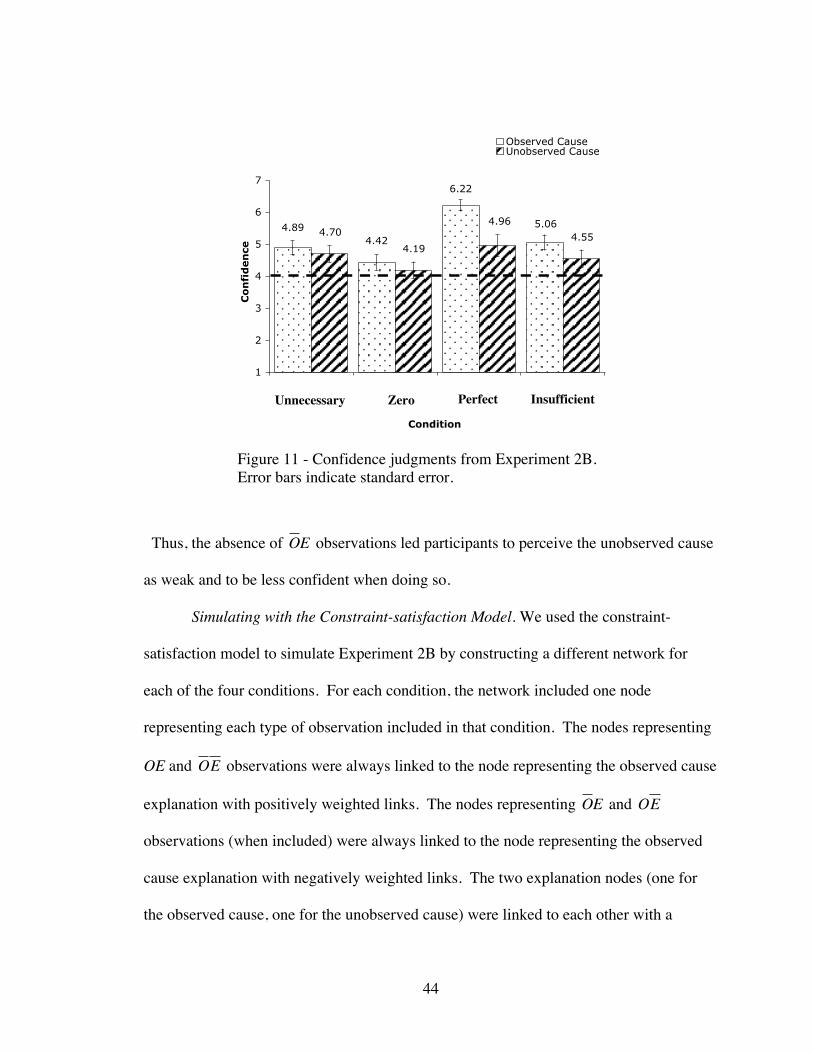
44

Thus, the absence of

€

OE observations led participants to perceive the unobserved cause

as weak and to be less confident when doing so.

Simulating with the Constraint-satisfaction Model. We used the constraint-

satisfaction model to simulate Experiment 2B by constructing a different network for

each of the four conditions. For each condition, the network included one node

representing each type of observation included in that condition. The nodes representing

OE and

€

OE observations were always linked to the node representing the observed cause

explanation with positively weighted links. The nodes representing

€

OE and

€

OE

observations (when included) were always linked to the node representing the observed

cause explanation with negatively weighted links. The two explanation nodes (one for

the observed cause, one for the unobserved cause) were linked to each other with a

Figure 11 - Confidence judgments from Experiment 2B.Error bars indicate standard error.

4.894.42

6.22

5.064.70

4.96

4.194.55

1

2

3

4

5

6

7

Condition

Confidence


Unnecessary Zero InsufficientPerfect

45

negatively weighted link. Additionally, the observation nodes were linked to a special

node whose activation was clamped at 1 (i.e., maximal).

The weights used were identical to those used in previous simulations and have

allowed such models to account for a range of both causal and non-causal judgments

(e.g., Thagard, 2000; Hagmeyer & Waldmann, 2002). Observation nodes and

explanation nodes were connected with links taking on positive weights of 0.05 or

negative weights of –0.05. The weight of the link between the explanation nodes was

–0.2. The activation of all nodes was then updated for 200 iterations (as in Thagard,

2000). The resulting activation of each explanation node (multiplied by 100 to match the

scale used by participants) was then taken as the judged strength of the cause.

The results of this simulation are displayed in the top panel of Figure 10. As

expected, the unobserved cause was predicted to be strongest in the Zero condition. In all

other conditions the model predicted that the unobserved cause would be perceived as

weaker. Unfortunately, these predictions are drastically different than the results of

Experiment 2B and provide a poor fit to the data (R2=.33, RMSD=88.84)10. The two

biggest errors made by the constraint-satisfaction model are not predicting an influence of

unexplained effects and the fact that the final activations tended towards the extremes

(i.e., 100 and -100).

10 In the C~E present/~CE present condition, all activation change is entirely due to theinitial, random activations (positive initial weights lead to positive final activations,negative initial weights lead to negative final activations). In the absence of these initialactivations, there are no changes in activation; the two explanations are in perfectequilibrium. Thus, in the absence of these random activations and assuming that peoplebegin the experiment believing that the causal strengths are zero (as BUCKLE and RWdo), the resulting activation of each explanation node should be zero.

46

Constraint-satisfaction models are traditionally able to take any beliefs a reasoner

might entertain and represent the complex interdependencies that related them (see

Thagard, 2000 for a wide array of applications). Why then does the constraint-

satisfaction model fail to account for the results of Experiment 2B? The constraint-

satisfaction model assumes that causes compete. This can be seen in the results of the

simulation. The unobserved cause explanation is maximally active in the Zero condition

in which there is an equal amount of positive (i.e., OE,

€

OE ) and negative (i.e.,

€

OE ,

€

OE )

support for the observed cause. In all other conditions, the unobserved cause explanation

is rejected because there is more evidence in favor of the observed cause explanation than

there is evidence against it. The adversarial relationship between causes/explanations is

useful for explaining causal judgments (see Morris & Larrick, 1995; Price & Yates,

1993), but it apparently cannot explain beliefs about unobserved alternative causes. For

example, participants believed both the observed and unobserved causes to be moderately

causal in both the Unnecessary and Insufficient conditions. This behavior leads us to

conclude that, without substantial additions, constraint-satisfaction models do not

accurately describe participants’ beliefs about unobserved causes.

Simulating with RW. Though Experiments 4-6 are more tailored to test RW, we

briefly summarize simulations conducted with RW. RW was assumed to learn about two

cues in the current experiment. The first, cueobs represents the observed cause. The other,

cuebg, represents an unobserved cause that is assumed to be present on every trial. We

simulated each of the conditions used in Experiment 2B (which used the methodology

appropriate to test RW) by presenting the model with the exact same set of observations

in the exact same order that participants received them. The final associative strength of

47

cueobs (multiplied by 100 to match the scale used by participants) was taken as the judged

strength of the observed cause. The final associative strength of cuebg (again multiplied

by 100) was taken as the judged strength of the unobserved cause. Because the

predictions of RW are quite sensitive to the learning rate, the learning rate, α, was fitted

to the data (again using the Hooke-Jeeves method). Additionally, to allow for the

possibility that the two cues were differentially salient, we fit a separate learning rate, α,

to each. The learning rate parameter associated with the outcome, β, was set to 0.5 for all

simulations. The best fitting parameters were 0.86 for cueobs and 0.62 for cuebg. The

estimates can be seen in the bottom panel of Figure 10. These estimates fit the data quite

well, (R2=.77, RMSD=21.97). These results will be discussed more thoroughly later.

Experiment 3

Experiments 2A and 2B demonstrated the importance of unexplained effects in

causal learning. The influence of unexplained effects was the most critical aspect of

BUCKLE’s predictions and set it apart from the constraint-satisfaction model. One

remaining question, however, involves the extent to which our methodology led

participants to be sensitive to unexplained effects. Participants in Experiment 2 were

given explicit information about the potential existence and influence of an unobserved

cause on every trial. As explained earlier, this measure was taken to equate participants’

assumptions about the learning environment with those of BUCKLE. Yet, this prior

knowledge may have inadvertently changed participants’ learning strategies with respect

to unobserved causes. That is, it is not clear from these experiments the extent to which

people make spontaneous inferences about unobserved causes. To explore how general

48

the influence of unexplained effects is, we conducted an additional experiment in which

participants were given no prior information about the existence of an unobserved cause.

Method

Fifty-two Yale University undergraduates participated for partial fulfillment of

course credit or $10/hour. Participants were randomly assigned to either the Explicit

condition (N=26) or the Implicit condition (N=26).

Stimulus materials and procedure was the same as in Experiment 2A except for

the following changes. Stimuli consisted of electrical systems like those used in previous

experiments. Instead of using all four contingencies, only two critical conditions were

used. These were the Unnecessary and Insufficient conditions (see Table 1).

Participants in the Explicit condition were told that there were two buttons and a

light as in Experiment 2. These participants were told that nothing else could affect the

light. In contrast, participants in the Implicit condition were told that the system included

one button and a light. Participants in the Implicit condition were not given any

information about the existence (or nonexistence) of alternative causes until they were

asked to evaluate their causal strengths after all observations were completed. All

participants were told that they would be asked to evaluate the causal strength of the

observed button. After viewing the entire set of trials participants in the Implicit

condition were told that the initial description of the system was incomplete. They were

told that the system actually contained a second button whose information had been lost

and that in each presented test any combination of these two buttons could have been

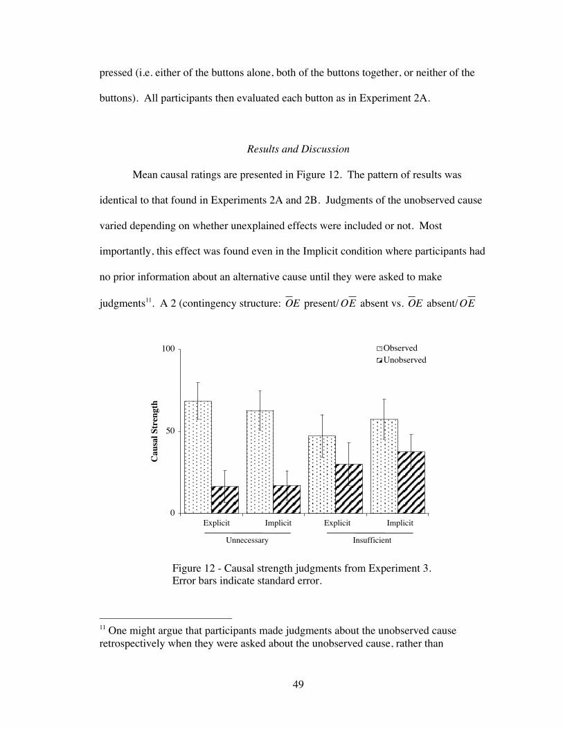
49

pressed (i.e. either of the buttons alone, both of the buttons together, or neither of the

buttons). All participants then evaluated each button as in Experiment 2A.


Mean causal ratings are presented in Figure 12. The pattern of results was

identical to that found in Experiments 2A and 2B. Judgments of the unobserved cause

varied depending on whether unexplained effects were included or not. Most

importantly, this effect was found even in the Implicit condition where participants had

no prior information about an alternative cause until they were asked to make

judgments11. A 2 (contingency structure:

€

OE present/

€

OE absent vs.

€

OE absent/

€

OE

11 One might argue that participants made judgments about the unobserved causeretrospectively when they were asked about the unobserved cause, rather than

Figure 12 - Causal strength judgments from Experiment 3.Error bars indicate standard error.

0

50

100

Cau

sal S

tren

gth

ObservedUnobserved

Explicit Implicit Explicit Implicit

InsufficientUnnecessary

50

present) X 2 (explicit / implicit) ANOVA was performed on the ratings of the unobserved

cause. This analysis revealed a significant main effect of contingency structure, F(1,

46)=21.28, p<.0001, because participants gave much higher ratings in the Unnecessary

condition (M = 65.58, SD = 40.75) than in the Insufficient condition (M = 16.75, SD =

31.53). Both the main effect of the instructional manipulation (i.e. level of implicitness)

and the interaction effect were non-significant (both F’s < 1).

The absence of an interaction between implicitness and contingency structure is

theoretically important because it suggests that people naturally learn about unobserved

causes12. Because of its importance, this effect was further subjected to a power analysis.

While our sample provided sufficient power (.81) to detect a “large” effect (i.e. f = .4),

the observed effect size was significantly smaller, f = .045. Achieving similar power to

detect an effect of this size would require an additional 3800 participants.

Summary

Experiments 2 and 3 demonstrate that judgments of unobserved causes are

systematic and vary depending on the contingency between the observed cause and the

effect. Unexplained effects were particularly influential. The unobserved cause was

perceived as strong only when participants encountered unexplained effects. Otherwise,

spontaneously making inferences about the unobserved cause during learning.Experiment 6 provides evidence against this interpretation.12 What exactly learners represent remains unclear. For example, it is unclear whetherpeople represent a single unobserved cause, as BUCKLE does, or whether they representmore than one. To explore this possibility, we modified BUCKLE so as to representmultiple unobserved causes. Though these modified versions of BUCKLE do makedifferent quantitative predictions, the effect is too subtle to draw any reasonableconclusions given the current result.

51

the unobserved cause was perceived as weak. BUCKLE, which is developed to be

sensitive to unexplained effects, obviously could explain such an effect.

These experiments did not, however, provide a critical comparison of BUCKLE

and RW. As explained earlier, RW represents an unobserved cause and assumes that it is

present at all times. The associative strength accrued by this cause matched Experiment

2B’s results quite well. Because of the apparent accuracy of RW’s account, we wish to

conduct a more thorough exploration into the details. We plan to test RW in three ways.

First, Experiment 4 and 5 will explore the difference between BUCKLE’s and RW’s

representation of unobserved causes. RW makes the assumption that the unobserved

cause is present at all times whereas BUCKLE computes the probability that the

unobserved cause is present for each observation. Second, RW is indifferent to the causal

role of events, whereas BUCKLE utilizes information about causal role. This critical

difference will be explained and tested in more detail in Experiment 6.

Experiment 4: Judging a Constant Cause

Though the unobserved cause in our experiments is certainly part of the

background, it seems unnatural to actually equate the two. The experimental context

includes the unobserved cause as well as other less obvious elements (e.g., the color of

the background during stimuli presentation). Thus, while causal judgments of the

unobserved cause should be related to the associative strength of the background, it is

unclear whether the two should be equal.

To explore this idea, we designed an experiment to evaluate the predictions of

RW more directly. Instead of being presented with an observed cause and an unobserved

52

cause as in previous experiments, participants in the experimental condition will be

presented with two observed causes. One cause will vary (i.e., sometimes present,

sometimes absent), whereas the other cause will always be present. We will then

compare participants’ judgments about the constantly present cause to their judgments of

an unobserved cause in the control condition. If people’s judgments of the unobserved

cause are based on the associative strength of the background context, then judgments of

the constant cause should be equal to judgments of the unobserved cause.

Method

Participants

Thirty-six Yale University undergraduates participated for partial fulfillment of

course credit or $10/hour.

Materials and Design

Stimuli consist of electrical systems like those used in previous experiments. The

experiment uses a 2 (contingency) X 2 (Unobserved vs. Constant cause) within-subject

design. Instead of using all four contingency structures, only two critical structures were

used. The contingencies will be the Unnecessary and Insufficient conditions (see Table

1), but will include ten trials of each type instead of seven as in Experiment 2. In the

Constant condition, one cause will be observed and vary according to the particular

contingency while the other will be observed and was present on every trial. In the

Unobserved condition one cause will be observed and vary according to the contingency

of the particular condition while the other cause will be unobserved (as in previous

experiments).

53

Procedure

The procedure was identical to that used in Experiment 2B.

Results

Results can be seen in Figure 13. The critical question in Experiment 4 is whether

people would evaluate the constant cause in the same manner as the unobserved cause.

We performed a 2 (condition: Unobserved vs. Constant) x 2 (contingency:

€

OE present/

absent vs.

€

OE present/ absent) repeated measures ANOVA on judgments of the

constant/unobserved causes. We observed a significant effect of condition (F(1,34)=8.39,

p<.01) because the causes were perceived as stronger in the Unobserved condition

(M=44.53) than in the Constant condition (M=13.42). We also observed a significant

effect of contingency (F(1,34)=27.45, p<.0001) because the causes were perceived as

stronger in the Unnecessary condition (M=57.42) than in the Insufficient condition

(M=0.53). The interaction between factors was not significant.

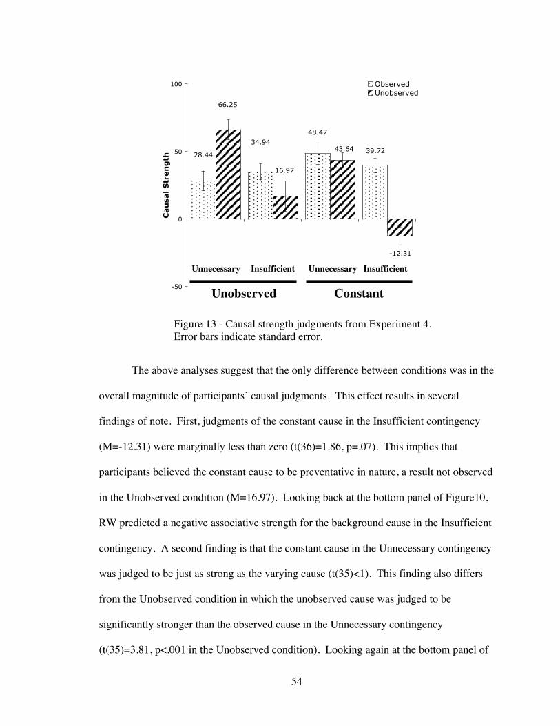
54

The above analyses suggest that the only difference between conditions was in the

overall magnitude of participants’ causal judgments. This effect results in several

findings of note. First, judgments of the constant cause in the Insufficient contingency

(M=-12.31) were marginally less than zero (t(36)=1.86, p=.07). This implies that

participants believed the constant cause to be preventative in nature, a result not observed

in the Unobserved condition (M=16.97). Looking back at the bottom panel of Figure10,

RW predicted a negative associative strength for the background cause in the Insufficient

contingency. A second finding is that the constant cause in the Unnecessary contingency

was judged to be just as strong as the varying cause (t(35)<1). This finding also differs

from the Unobserved condition in which the unobserved cause was judged to be

significantly stronger than the observed cause in the Unnecessary contingency

(t(35)=3.81, p<.001 in the Unobserved condition). Looking again at the bottom panel of

Figure 13 - Causal strength judgments from Experiment 4.Error bars indicate standard error.

28.44

34.9439.72

48.47

-12.31

43.64

16.97

66.25

-50

0

50

100

Cau

sal S

tren

gth

ObservedUnobserved

UnnecessaryUnnecessary Insufficient Insufficient

ConstantUnobserved

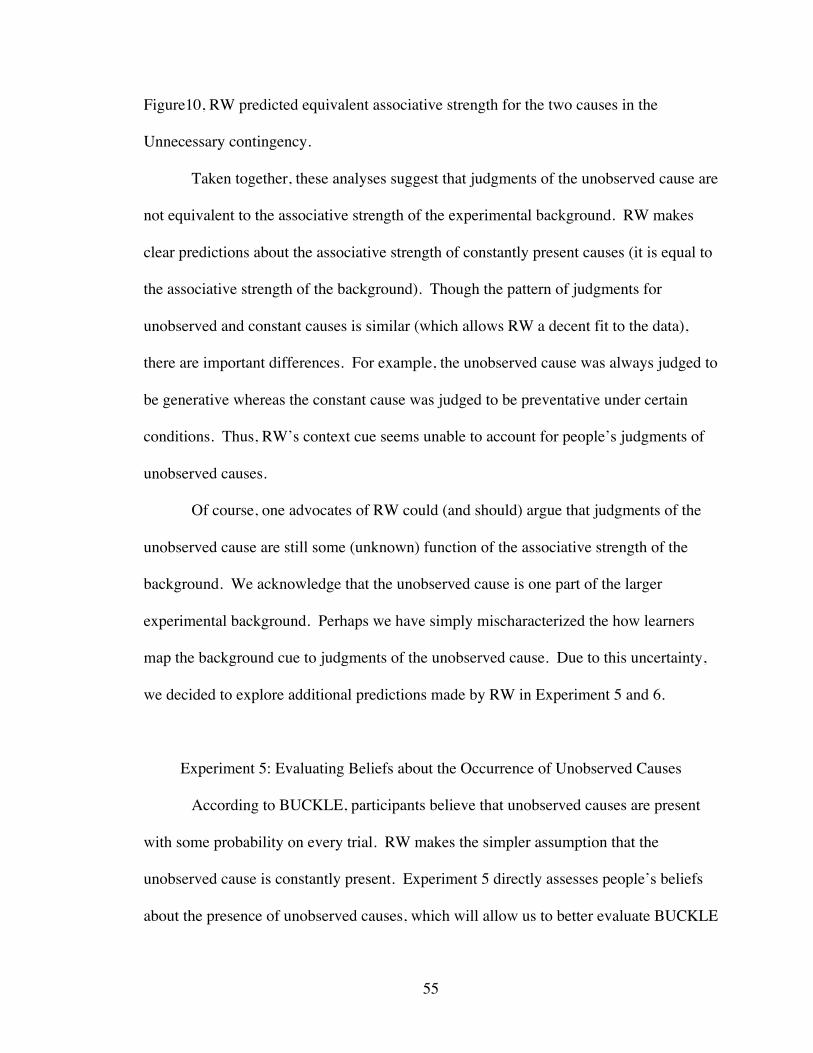
55

Figure10, RW predicted equivalent associative strength for the two causes in the

Unnecessary contingency.

Taken together, these analyses suggest that judgments of the unobserved cause are

not equivalent to the associative strength of the experimental background. RW makes

clear predictions about the associative strength of constantly present causes (it is equal to

the associative strength of the background). Though the pattern of judgments for

unobserved and constant causes is similar (which allows RW a decent fit to the data),

there are important differences. For example, the unobserved cause was always judged to

be generative whereas the constant cause was judged to be preventative under certain

conditions. Thus, RW’s context cue seems unable to account for people’s judgments of

unobserved causes.

Of course, one advocates of RW could (and should) argue that judgments of the

unobserved cause are still some (unknown) function of the associative strength of the

background. We acknowledge that the unobserved cause is one part of the larger

experimental background. Perhaps we have simply mischaracterized the how learners

map the background cue to judgments of the unobserved cause. Due to this uncertainty,

we decided to explore additional predictions made by RW in Experiment 5 and 6.

Experiment 5: Evaluating Beliefs about the Occurrence of Unobserved Causes

According to BUCKLE, participants believe that unobserved causes are present

with some probability on every trial. RW makes the simpler assumption that the

unobserved cause is constantly present. Experiment 5 directly assesses people’s beliefs

about the presence of unobserved causes, which will allow us to better evaluate BUCKLE

56

and RW. Experiment 5 was similar to Experiment 2; on every trial, participants were

presented with information about the presence or absence of one of the causes and the

effect while the second cause remained unobserved. However, unlike Experiment 2,

participants were asked to rate the probability that the unobserved cause was present on

that trial.

As explained in the introduction, BUCKLE predicts that the probability of the

unobserved cause will vary as a function of type of evidence (e.g., OE or

€

OE ) as well as

qu and qo. More detailed predictions of BUCKLE will be presented later. In short, the

main goal of Experiment 5 was to demonstrate that (1) people’s estimates of P(u|,o,e) in a

given learning situation vary as a function of type of evidence and (2) the same type of

observation can lead to different estimates of P(u|,o,e) as a function of qu and qo.

In addition, because Experiment 5 provides direct assessments of P(u|o,e), it

allows us to examine whether people are making the no-confounding assumption (i.e.,

P(u|o) = P(u|~o)) required by the Power PC theory. If participants do not believe this

assumption met, the Power PC theory cannot estimate causal power and people should be

unable to provide causal strength judgments (Cheng, 1997). In contrast, BUCKLE does

not require such a constraint in learning of observed causes. Hagmeyer and Waldmann

(2004) demonstrated that learners make causal judgments even when they believe the no-

confounding assumption to be violated. Unfortunately, Hagmeyer and Waldmann use

only a small variety of contingencies and they do not report data relevant to our test of

BUCKLE (e.g., P(u|o) and P(u|~o)). Thus, Experiment 5 seeks to use a wider range of

contingencies and will allow a better test of BUCKLE.

57

Method

Participants

Twenty-four Vanderbilt University undergraduates participated for partial

fulfillment of course credit.

Materials and Procedure

Stimuli consisted of four electrical systems used in Experiment 2. The design was

the same as in Experiment 2 (Table 1) except that, in order to increase the number of

measurements taken, we presented each cell 10 times instead of the original 7.

The procedure of Experiment 5 was the same as in Experiment 2A except for the

following addition. After the trial information was presented and the spacebar was

pressed to continue, a question appeared on the screen below the depiction of that trial.

The question was, “How likely is it that the [color] button was pressed in this test?”

where the button referred was the unobserved cause. Below this was an eleven-point

scale ranging from 0 (Definitely NOT pressed) to 10 (Definitely pressed). After typing

their answer on the computer keyboard, the next trial commenced. It should be noted that

asking participants about the probability of the unobserved cause on every trial did not

appear to have created an unusually disruptive learning situation, because the pattern of

causal strength judgments (see Figure 14) mirrored that of Experiment 213.

13 A 2 (

€

OEpresent / absent) X 2 (

€

OEpresent / absent) repeated measures ANOVA oncausal judgments of unobserved causes revealed a significant main effect of

€

OEinformation, F(1, 22) = 26.59, p<.0001, because participants gave much higher ratings onconditions with

€

OE (M = 72.60, SD = 28.77) than on conditions without

€

OE (M =41.47, SD = 35.69). No other main effects or interactions were significant.

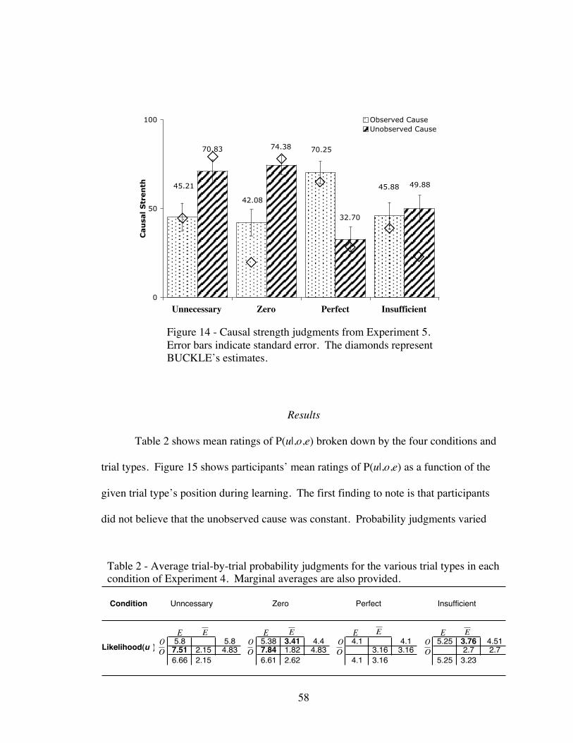
58

Results

Table 2 shows mean ratings of P(u|,o,e) broken down by the four conditions and

trial types. Figure 15 shows participants’ mean ratings of P(u|,o,e) as a function of the

given trial type’s position during learning. The first finding to note is that participants

did not believe that the unobserved cause was constant. Probability judgments varied

5.8 5.8 5.38 3.41 4.4 4.1 4.1 5.25 3.76 4.517.51 2.15 4.83 7.84 1.82 4.83 3.16 3.16 2.7 2.76.66 2.15 6.61 2.62 4.1 3.16 5.25 3.23

Unncessary Perfect InsufficientZeroCondition

Likelihood(u )

€

E

€

O

€

O

€

E

€

E

€

O

€

O

€

E

€

E

€

O

€

O

€

E

€

E

€

O

€

O

€

E

Table 2 - Average trial-by-trial probability judgments for the various trial types in eachcondition of Experiment 4. Marginal averages are also provided.

Figure 14 - Causal strength judgments from Experiment 5.Error bars indicate standard error. The diamonds representBUCKLE’s estimates.

45.21

42.08

45.88

70.2570.83 74.38

32.70

49.88

0

50

100

Cau

sal

Str

en

th


Unnecessary Zero Perfect Insufficient

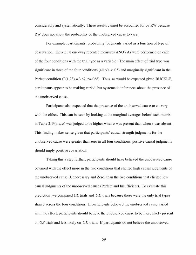
59

considerably and systematically. These results cannot be accounted for by RW because

RW does not allow the probability of the unobserved cause to vary.

For example, participants’ probability judgments varied as a function of type of

observation. Individual one-way repeated measures ANOVAs were performed on each

of the four conditions with the trial type as a variable. The main effect of trial type was

significant in three of the four conditions (all p’s < .05) and marginally significant in the

Perfect condition (F(1,23) = 3.67, p=.068). Thus, as would be expected given BUCKLE,

participants appear to be making varied, but systematic inferences about the presence of

the unobserved cause.

Participants also expected that the presence of the unobserved cause to co-vary

with the effect. This can be seen by looking at the marginal averages below each matrix

in Table 2; P(u|,o,e) was judged to be higher when e was present than when e was absent.

This finding makes sense given that participants’ causal strength judgments for the

unobserved cause were greater than zero in all four conditions; positive causal judgments

should imply positive covariation.

Taking this a step further, participants should have believed the unobserved cause

covaried with the effect more in the two conditions that elicited high causal judgments of

the unobserved cause (Unnecessary and Zero) than the two conditions that elicited low

causal judgments of the unobserved cause (Perfect and Insufficient). To evaluate this

prediction, we compared OE trials and

€

OE trials because these were the only trial types

shared across the four conditions. If participants believed the unobserved cause varied

with the effect, participants should believe the unobserved cause to be more likely present

on OE trials and less likely on

€

OE trials. If participants do not believe the unobserved

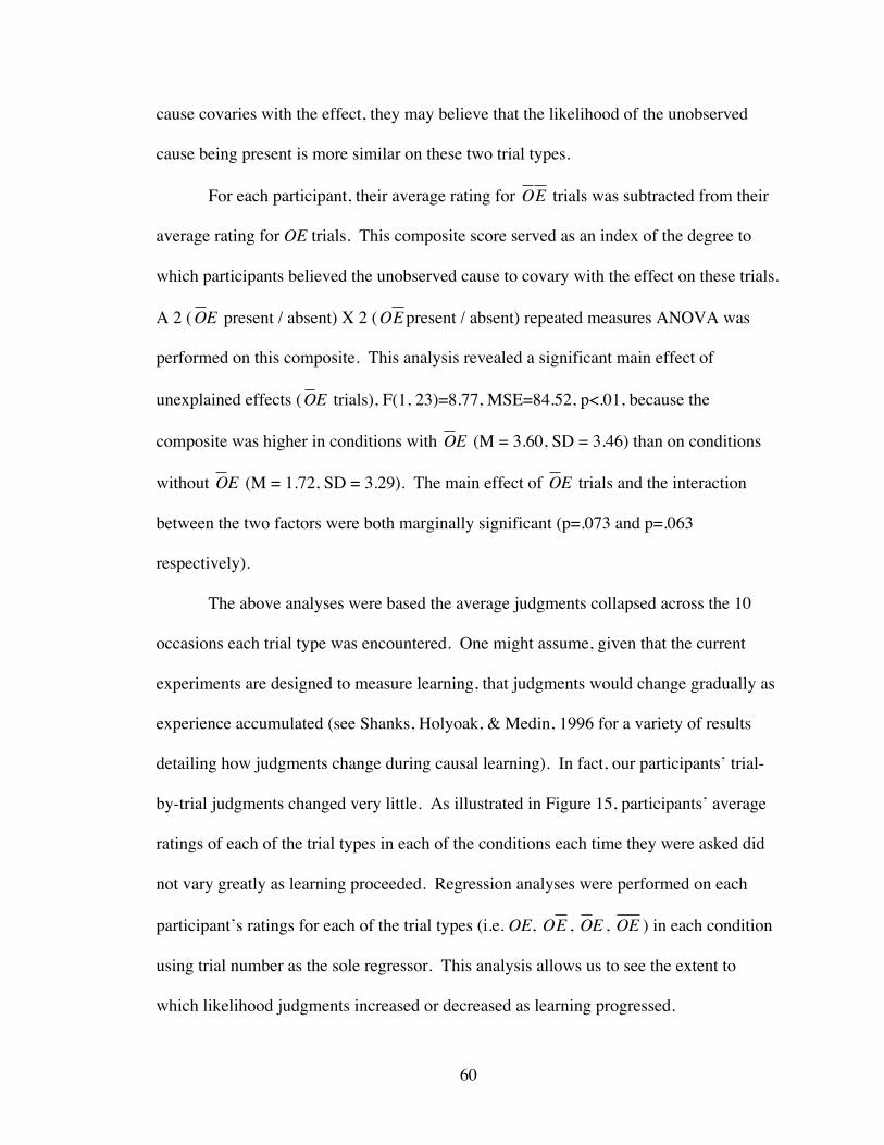
60

cause covaries with the effect, they may believe that the likelihood of the unobserved

cause being present is more similar on these two trial types.

For each participant, their average rating for

€

OE trials was subtracted from their

average rating for OE trials. This composite score served as an index of the degree to

which participants believed the unobserved cause to covary with the effect on these trials.

A 2 (

€


€

OEpresent / absent) repeated measures ANOVA was

performed on this composite. This analysis revealed a significant main effect of

unexplained effects (

€

OE trials), F(1, 23)=8.77, MSE=84.52, p<.01, because the

composite was higher in conditions with

€

OE (M = 3.60, SD = 3.46) than on conditions

without

€

OE (M = 1.72, SD = 3.29). The main effect of

€

OE trials and the interaction

between the two factors were both marginally significant (p=.073 and p=.063

respectively).

The above analyses were based the average judgments collapsed across the 10

occasions each trial type was encountered. One might assume, given that the current

experiments are designed to measure learning, that judgments would change gradually as

experience accumulated (see Shanks, Holyoak, & Medin, 1996 for a variety of results

detailing how judgments change during causal learning). In fact, our participants’ trial-

by-trial judgments changed very little. As illustrated in Figure 15, participants’ average

ratings of each of the trial types in each of the conditions each time they were asked did

not vary greatly as learning proceeded. Regression analyses were performed on each

participant’s ratings for each of the trial types (i.e. OE,

€

OE ,

€

OE ,

€

OE ) in each condition

using trial number as the sole regressor. This analysis allows us to see the extent to

which likelihood judgments increased or decreased as learning progressed.

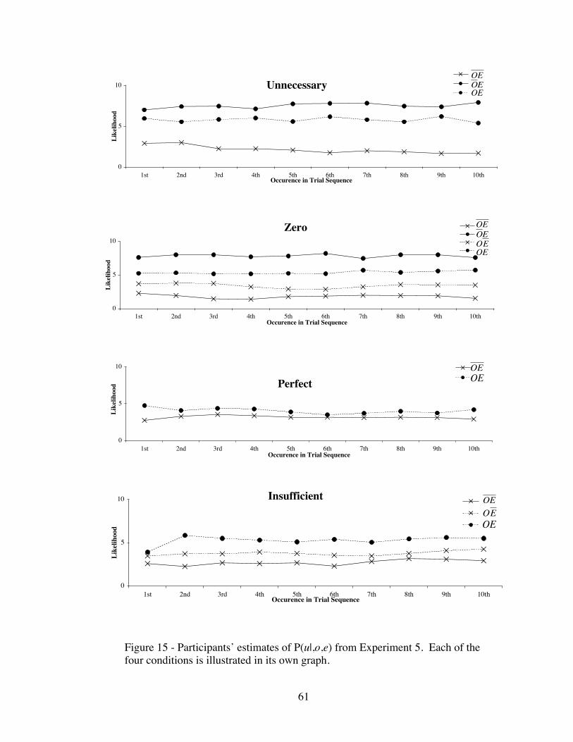
61

0

5

10

1st 2nd 3rd 4th 5th 6th 7th 8th 9th 10thOccurence in Trial Sequence

Like

lihoo

d€

OE

€

OE

€

OEUnnecessary

0

5

10


Like

lihoo

d

€

OE

€

OE€

OE

€

OE

Zero

0

5

10


Like

lihoo

d

€

OE

€

OE

Perfect

0

5

10


Like

lihoo

d

€

OE

€

OE€

OEInsufficient

Figure 15 - Participants’ estimates of P(u|,o,e) from Experiment 5. Each of thefour conditions is illustrated in its own graph.

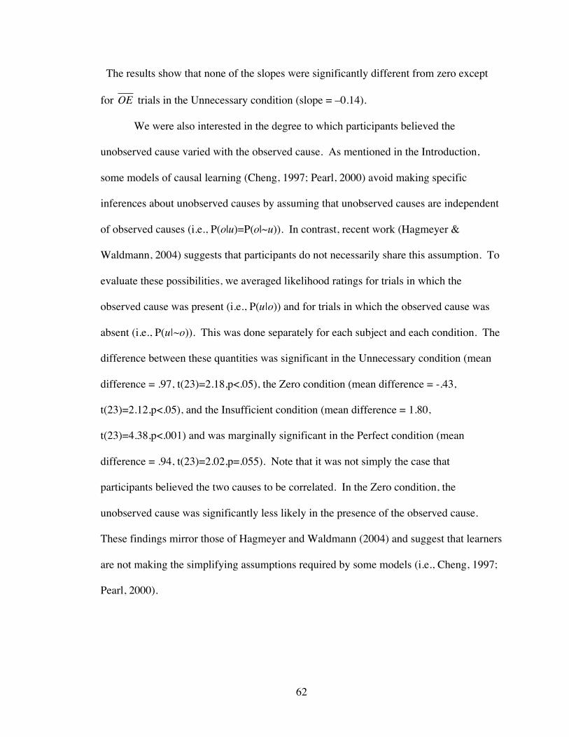
62

The results show that none of the slopes were significantly different from zero except

for

€

OE trials in the Unnecessary condition (slope = –0.14).

We were also interested in the degree to which participants believed the

unobserved cause varied with the observed cause. As mentioned in the Introduction,

some models of causal learning (Cheng, 1997; Pearl, 2000) avoid making specific

inferences about unobserved causes by assuming that unobserved causes are independent

of observed causes (i.e., P(o|u)=P(o|~u)). In contrast, recent work (Hagmeyer &

Waldmann, 2004) suggests that participants do not necessarily share this assumption. To

evaluate these possibilities, we averaged likelihood ratings for trials in which the

observed cause was present (i.e., P(u|o)) and for trials in which the observed cause was

absent (i.e., P(u|~o)). This was done separately for each subject and each condition. The

difference between these quantities was significant in the Unnecessary condition (mean

difference = .97, t(23)=2.18,p<.05), the Zero condition (mean difference = -.43,

t(23)=2.12,p<.05), and the Insufficient condition (mean difference = 1.80,

t(23)=4.38,p<.001) and was marginally significant in the Perfect condition (mean

difference = .94, t(23)=2.02,p=.055). Note that it was not simply the case that

participants believed the two causes to be correlated. In the Zero condition, the

unobserved cause was significantly less likely in the presence of the observed cause.

These findings mirror those of Hagmeyer and Waldmann (2004) and suggest that learners

are not making the simplifying assumptions required by some models (i.e., Cheng, 1997;

Pearl, 2000).

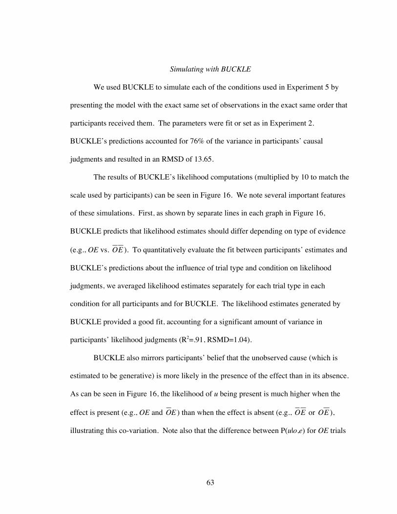
63

Simulating with BUCKLE

We used BUCKLE to simulate each of the conditions used in Experiment 5 by

presenting the model with the exact same set of observations in the exact same order that

participants received them. The parameters were fit or set as in Experiment 2.

BUCKLE’s predictions accounted for 76% of the variance in participants’ causal

judgments and resulted in an RMSD of 13.65.

The results of BUCKLE’s likelihood computations (multiplied by 10 to match the

scale used by participants) can be seen in Figure 16. We note several important features

of these simulations. First, as shown by separate lines in each graph in Figure 16,

BUCKLE predicts that likelihood estimates should differ depending on type of evidence

(e.g., OE vs.

€

OE ). To quantitatively evaluate the fit between participants’ estimates and

BUCKLE’s predictions about the influence of trial type and condition on likelihood

judgments, we averaged likelihood estimates separately for each trial type in each

condition for all participants and for BUCKLE. The likelihood estimates generated by

BUCKLE provided a good fit, accounting for a significant amount of variance in

participants’ likelihood judgments (R2=.91, RSMD=1.04).

BUCKLE also mirrors participants’ belief that the unobserved cause (which is

estimated to be generative) is more likely in the presence of the effect than in its absence.

As can be seen in Figure 16, the likelihood of u being present is much higher when the

effect is present (e.g., OE and

€

OE ) than when the effect is absent (e.g.,

€

OE or

€

OE ),

illustrating this co-variation. Note also that the difference between P(u|o,e) for OE trials

64

and P(u|o,e) for

€

OE trials is fairly large in these two conditions. In contrast, the bottom

two panels show conditions where qu was only somewhat positive.

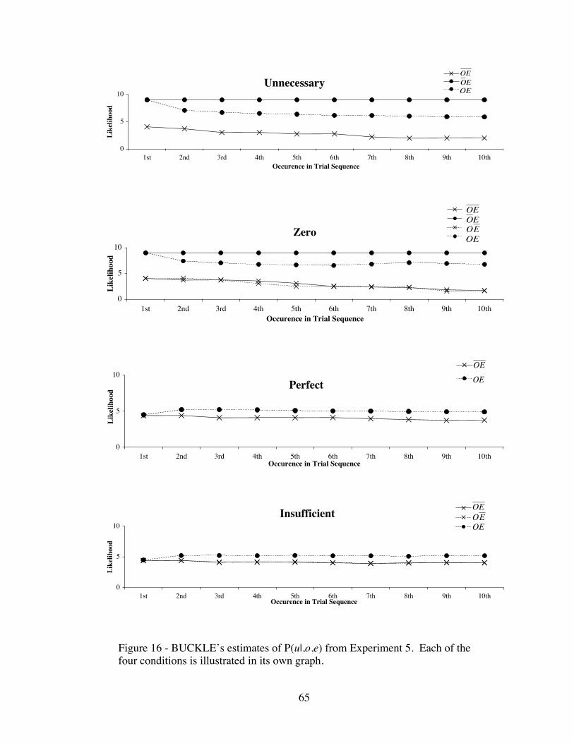
65

0

5

10


Like

lihoo

d€

OE

€

OE

€

OEUnnecessary

0

5

10


Like

lihoo

d €

OE

€

OE

€

OE

€

OEZero

0

5

10


Like

lihoo

d

€

OE

€

OEPerfect

0

5

10


Like

lihoo

d

€

OE

€

OE

€

OEInsufficient

Figure 16 - BUCKLE’s estimates of P(u|,o,e) from Experiment 5. Each of thefour conditions is illustrated in its own graph.

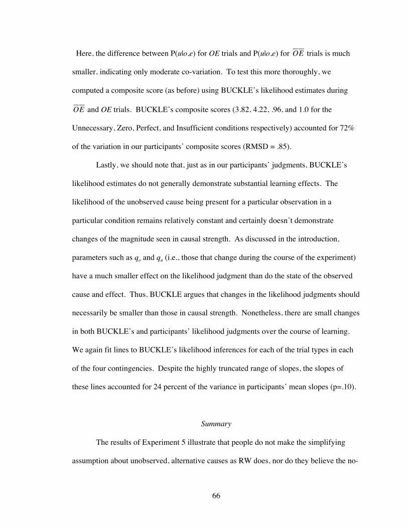
66

Here, the difference between P(u|o,e) for OE trials and P(u|o,e) for

€

OE trials is much

smaller, indicating only moderate co-variation. To test this more thoroughly, we

computed a composite score (as before) using BUCKLE’s likelihood estimates during

€

OE and OE trials. BUCKLE’s composite scores (3.82, 4.22, .96, and 1.0 for the

Unnecessary, Zero, Perfect, and Insufficient conditions respectively) accounted for 72%

of the variation in our participants’ composite scores (RMSD = .85).

Lastly, we should note that, just as in our participants’ judgments, BUCKLE’s

likelihood estimates do not generally demonstrate substantial learning effects. The

likelihood of the unobserved cause being present for a particular observation in a

particular condition remains relatively constant and certainly doesn’t demonstrate

changes of the magnitude seen in causal strength. As discussed in the introduction,

parameters such as qo and qu (i.e., those that change during the course of the experiment)

have a much smaller effect on the likelihood judgment than do the state of the observed

cause and effect. Thus, BUCKLE argues that changes in the likelihood judgments should

necessarily be smaller than those in causal strength. Nonetheless, there are small changes

in both BUCKLE’s and participants’ likelihood judgments over the course of learning.

We again fit lines to BUCKLE’s likelihood inferences for each of the trial types in each

of the four contingencies. Despite the highly truncated range of slopes, the slopes of

these lines accounted for 24 percent of the variance in participants’ mean slopes (p=.10).

Summary

The results of Experiment 5 illustrate that people do not make the simplifying

assumption about unobserved, alternative causes as RW does, nor do they believe the no-

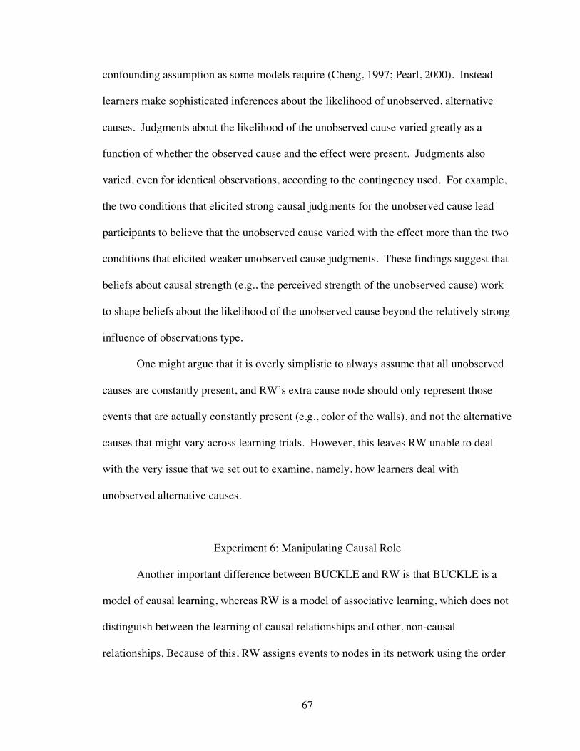
67

confounding assumption as some models require (Cheng, 1997; Pearl, 2000). Instead

learners make sophisticated inferences about the likelihood of unobserved, alternative

causes. Judgments about the likelihood of the unobserved cause varied greatly as a

function of whether the observed cause and the effect were present. Judgments also

varied, even for identical observations, according to the contingency used. For example,

the two conditions that elicited strong causal judgments for the unobserved cause lead

participants to believe that the unobserved cause varied with the effect more than the two

conditions that elicited weaker unobserved cause judgments. These findings suggest that

beliefs about causal strength (e.g., the perceived strength of the unobserved cause) work

to shape beliefs about the likelihood of the unobserved cause beyond the relatively strong

influence of observations type.

One might argue that it is overly simplistic to always assume that all unobserved

causes are constantly present, and RW’s extra cause node should only represent those

events that are actually constantly present (e.g., color of the walls), and not the alternative

causes that might vary across learning trials. However, this leaves RW unable to deal

with the very issue that we set out to examine, namely, how learners deal with

unobserved alternative causes.

Experiment 6: Manipulating Causal Role

Another important difference between BUCKLE and RW is that BUCKLE is a

model of causal learning, whereas RW is a model of associative learning, which does not

distinguish between the learning of causal relationships and other, non-causal

relationships. Because of this, RW assigns events to nodes in its network using the order

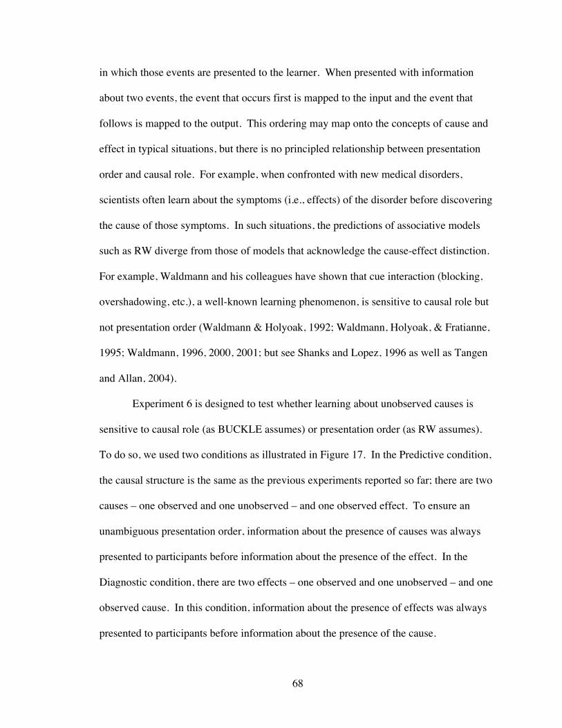
68

in which those events are presented to the learner. When presented with information

about two events, the event that occurs first is mapped to the input and the event that

follows is mapped to the output. This ordering may map onto the concepts of cause and

effect in typical situations, but there is no principled relationship between presentation

order and causal role. For example, when confronted with new medical disorders,

scientists often learn about the symptoms (i.e., effects) of the disorder before discovering

the cause of those symptoms. In such situations, the predictions of associative models

such as RW diverge from those of models that acknowledge the cause-effect distinction.

For example, Waldmann and his colleagues have shown that cue interaction (blocking,

overshadowing, etc.), a well-known learning phenomenon, is sensitive to causal role but

not presentation order (Waldmann & Holyoak, 1992; Waldmann, Holyoak, & Fratianne,

1995; Waldmann, 1996, 2000, 2001; but see Shanks and Lopez, 1996 as well as Tangen

and Allan, 2004).

Experiment 6 is designed to test whether learning about unobserved causes is

sensitive to causal role (as BUCKLE assumes) or presentation order (as RW assumes).

To do so, we used two conditions as illustrated in Figure 17. In the Predictive condition,

the causal structure is the same as the previous experiments reported so far; there are two

causes – one observed and one unobserved – and one observed effect. To ensure an

unambiguous presentation order, information about the presence of causes was always

presented to participants before information about the presence of the effect. In the

Diagnostic condition, there are two effects – one observed and one unobserved – and one

observed cause. In this condition, information about the presence of effects was always

presented to participants before information about the presence of the cause.

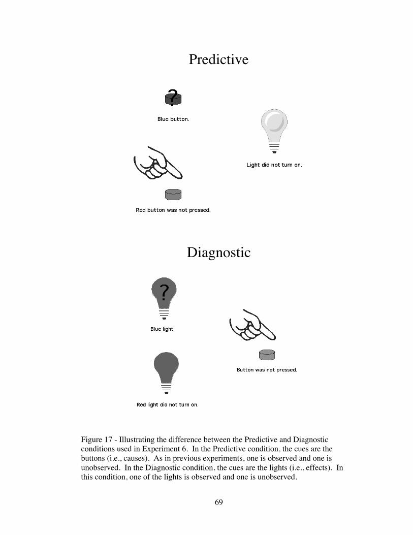
69

Figure 17 - Illustrating the difference between the Predictive and Diagnosticconditions used in Experiment 6. In the Predictive condition, the cues are thebuttons (i.e., causes). As in previous experiments, one is observed and one isunobserved. In the Diagnostic condition, the cues are the lights (i.e., effects). Inthis condition, one of the lights is observed and one is unobserved.

Predictive

Diagnostic

70

According to RW, these two conditions are identical; “for an associative account,

however, the real-world interpretation of the events is immaterial” (Shanks, Lopez,

Darby, Dickinson, 1996, p. 281). Therefore, if people’s judgments in the Diagnostic

differ from those in the Predictive conditions, RW will be unable to explain why this is

the case.

Yet, an attempt has been made in the associative camp to devise a way to be

sensitive to causal role. Shanks and Lopez (1996) proposed that diagnostic learning takes

place by running two associative networks in parallel. One network would learn

according to presentation order (effects to causes) and one according to causal role

(causes to effects). On this account, which network’s weights are used to generate

judgments is based entirely on the judgment being elicited. If the learner is asked to

make a judgment based on presentation order, then the learner uses the network that

tracked presentation order as traditionally modeled. If, on the other hand, the learner is

asked to make a judgment based on causal role (a diagnostic judgment), then the learner

uses the network that tracked causal roles. To avoid this possibility, Experiment 6

elicited judgments based on presentation order following Waldmann (2001): In both the

Diagnostic and Predictive conditions, participants were asked about the degree to which

each of the first events predicted the second. This methodological detail disallows

participants from using their knowledge of causal roles. In the Diagnostic condition in

particular, participants were asked about the degree to which the presence of the effect

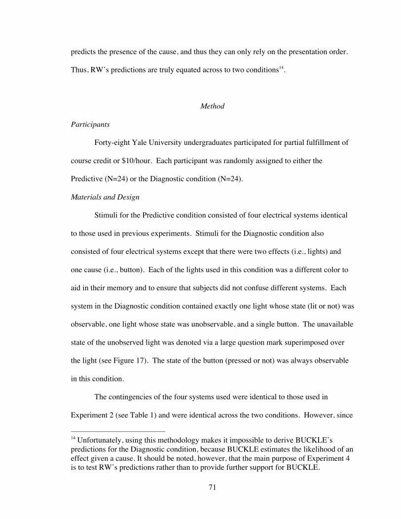
71

predicts the presence of the cause, and thus they can only rely on the presentation order.

Thus, RW’s predictions are truly equated across to two conditions14.

Method

Participants

Forty-eight Yale University undergraduates participated for partial fulfillment of

course credit or $10/hour. Each participant was randomly assigned to either the

Predictive (N=24) or the Diagnostic condition (N=24).

Materials and Design

Stimuli for the Predictive condition consisted of four electrical systems identical

to those used in previous experiments. Stimuli for the Diagnostic condition also

consisted of four electrical systems except that there were two effects (i.e., lights) and

one cause (i.e., button). Each of the lights used in this condition was a different color to

aid in their memory and to ensure that subjects did not confuse different systems. Each

system in the Diagnostic condition contained exactly one light whose state (lit or not) was

observable, one light whose state was unobservable, and a single button. The unavailable

state of the unobserved light was denoted via a large question mark superimposed over

the light (see Figure 17). The state of the button (pressed or not) was always observable

in this condition.

The contingencies of the four systems used were identical to those used in

Experiment 2 (see Table 1) and were identical across the two conditions. However, since

14 Unfortunately, using this methodology makes it impossible to derive BUCKLE’spredictions for the Diagnostic condition, because BUCKLE estimates the likelihood of aneffect given a cause. It should be noted, however, that the main purpose of Experiment 4is to test RW’s predictions rather than to provide further support for BUCKLE.

72

the causal role is reversed in the Diagnostic condition, instead of naming the independent

variables in terms of o and e (which stand for observed cause and effect) we will refer

them in terms of Cue and Outcome (i.e.,

€

Cue ⋅Outcome present or absent, and

€

Cue ⋅Outcome present or absent). Thus, the experiment is a 2 (

€

Cue ⋅Outcome :

present/absent) X 2 (

€

Cue ⋅Outcome : present/absent) X 2 (Predictive versus Diagnostic

conditions) mixed design with the last factor being manipulated between subjects.

Procedure

The procedure was similar to that used in Experiment 2. Participants saw all four

systems in a counterbalanced order. Trials for each system were presented in quasi-

random order. One difference between this and previous experiments was the

presentation of individual trials. Because RW uses presentation order to determine the

difference between input and output, we wanted to make the presentation order as

unambiguous as possible. Thus, for all trials, the first event (i.e., causes in the Predictive

condition and effects in the Diagnostic condition) was presented in isolation for 250ms.

After this delay, the second event (i.e., the effect in the Predictive condition and the cause

in the Diagnostic condition) was presented alongside the first event. At this point the

participant was able to press a key to proceed to the next trial at her own pace.

After viewing the entire set of trials for a single system, participants were asked to

provide responses. To allow identical dependent variables for the two conditions, we

elicited predictive judgments (i.e., how well one of the first events predicted the second;

Waldmann, 2001). Thus, in the Predictive condition, participants were asked, “How well

does the [color] button being pressed predict whether or not the light turned on?” In the

Diagnostic condition, participants were asked, “How well does the [color] light turning

73

on predict whether or not the button had been pressed?” Judgments were made on a scale

ranging from 0 (labeled as “Not at all a predictor”) to 100 (labeled as “A perfect

predictor”). These responses were obtained for both the observed and the unobserved

events.

74

Figure 18 - Results from Experiment 6. The results in the Predictivecondition mirror those found in the other experiments. The results in theDiagnostic condition look quite different. RW cannot account for thisdifference.

Predictive

54.21

96.63

18.54

39.21

52.71

10.96

76.67

69.50

0

50

100

Cau

sal

Str

en

gth

ObservedUnobserved


Diagnostic

52.63

31.75

94.50

37.92

31.67

23.33

31.88 34.21

0

50

100

Cau

sal S

tren

gth

ObservedUnobserved


75

Results

Participants’ mean ratings for both the observed and the unobserved events can be

seen in Figure 18. To investigate how causal role influenced judgments of the

unobserved event, we performed a 2 (Condition: Predictive / Diagnostic) X 2

(

€

Cue ⋅Outcome : present/absent) X 2 (

€

Cue ⋅Outcome : present/absent) ANOVA with

repeated measures on the last two factors over participants’ ratings on the unobserved

event. The critical question was whether the Predictive /Diagnostic manipulation would

influence judgments. This analysis revealed a significant main effect of condition

(F(1,46)=16.28, p<.0005) and this factor interacted with both the presence of

€

Cue ⋅Outcome (F(1,46)=46.12, p<.0001) and

€

Cue ⋅Outcome (F(1,46)=14.06, p<.001).

That is, the causal role of events had a significant effect on judgments.

To better understand this pattern of results, we performed individual 2

(

€

Cue ⋅Outcome : present/absent) X 2 (

€

Cue ⋅Outcome : present/absent) ANOVAs for each

condition. For the Predictive condition, the main effect of

€

Cue ⋅Outcome observations

was significant (F(1,23)=59.83, p<.0001) because systems including

€

Cue ⋅Outcome

observations elicited higher unobserved cause judgment (M = 73.08, SD = 30.38) than

those not including

€

Cue ⋅Outcome observations (M = 31.83, SD = 30.97). In other

words, the previous effect of unexplained effects was replicated. The main effect of

€

Cue ⋅Outcome observations was also significant (F(1,23)=18.78, p<.0005) because

conditions that included

€

Cue ⋅Outcome observations elicited higher unobserved cause

judgments (M =64.69, SD = 29.42) than those that did not (M = 40.23, SD = 39.76). The

interaction between these factors was also significant (F(1,23)=15.48, p<.001). For the

76

Diagnostic condition, we again performed a 2 (

€

Cue ⋅Outcome : present / absent) X 2

(

€

Cue ⋅Outcome : present / absent) ANOVA, but found no significant effects, all p’s > .2.

These analyses make it clear that, contrary to the predictions of RW, judgments of

unobserved events are greatly influenced by the manipulated causal role. In the

Predictive condition, judgments of the unobserved cause varied with the contingency as

predicted by BUCKLE. In the Diagnostic condition, however, no such effect was found.

Instead, judgments were uniformly low regardless of observed contingency, suggesting

that people do not spontaneously make inferences about unobserved effects in the same

way they do about unobserved causes. Indeed, the lack of learning about unobserved

effects is reasonable given that there appears to be no basis for making educated

judgments about the unobserved effects.

To summarize, Experiment 6 investigated whether learning about unobserved

events is a general feature of learning, as one would assume given RW’s representation,

or whether inferences about likelihood and strength are sensitive to causal role.

Confronted with a diagnostic learning situation (i.e., effects predicting their causes),

participants’ behavior deviated significantly from that in the Predictive condition (and

from the results of experiments reported above). From an associative perspective, this

difference is inexplicable because causal role should be irrelevant for learning. In

contrast, causal role is critical for BUCKLE’s inferences. For example, the likelihood of

an effect occurring after its cause cannot be equated with the likelihood of a cause

preceding its effect. The results of Experiment 6 suggest that causal role is an important

determinant of learning about unobserved, alternative causes.

77

Experiment 7: Order-effects

One critical aspect of the causal learning process described by BUCKLE is that

causal strength estimates are updated in a sequential manner as each observation is made.

This approach contrasts with approaches that compute causal strength over all available

trials once enough observations have been accumulated (e.g., Cheng, 1997; Busemeyer,

1991; White, 2002). According to BUCKLE, however, people’s inferences about the

likelihood of the unobserved cause changes as a function of the variables qu, and qo,

which change over the course of learning. An interesting consequence of this is that the

order in which observations are encountered should influence the final causal strength

estimates because identical observations will be interpreted differently depending on qu

and qo, which in turn would change beliefs about qu and qo (e.g., Dennis & Ahn, 2001).

To demonstrate this effect, we used the set of trials summarized in the top panel in

Figure 19. This set of trials was divided into two blocks. One of the blocks contained

unexplained effects (

€

OE ) and the other did not. These two blocks could be ordered in

one of two ways; the block containing unexplained effects could be presented either first

(early-unexplained-effect condition) or second (late-unexplained-effect condition) as

shown in the bottom panel in Figure 19. Note that, because the only manipulation was

the order of the two blocks, participants always saw the same set of observations by the

end of the sequence. Thus, any differences between conditions cannot be a result of the

number or type of trials observed.

BUCKLE predicts that the causal strength judgments will differ between the two

orderings. To see why this is, consider the early-unexplained-effect condition. During

the first block of this condition, the unexplained effects will lead to the unobserved cause

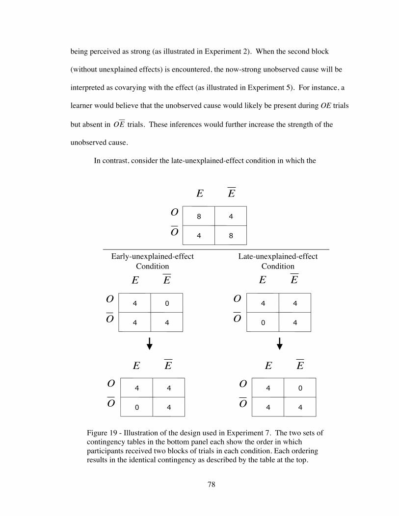
78

being perceived as strong (as illustrated in Experiment 2). When the second block

(without unexplained effects) is encountered, the now-strong unobserved cause will be

interpreted as covarying with the effect (as illustrated in Experiment 5). For instance, a

learner would believe that the unobserved cause would likely be present during OE trials

but absent in

€

OE trials. These inferences would further increase the strength of the

unobserved cause.

In contrast, consider the late-unexplained-effect condition in which the

8 4

4 8

4 0 4 4

4 4 0 4

€

O

€

O€

E

€

E

€

O

€

O€

E

€

E

€

O

€

O€

E

€

E

Early-unexplained-effectCondition

4 0

4 4

€

O

€

O€

E

€

E

4 4

0 4

€

O

€

O€

E

€

E

Late-unexplained-effectCondition

Figure 19 - Illustration of the design used in Experiment 7. The two sets ofcontingency tables in the bottom panel each show the order in whichparticipants received two blocks of trials in each condition. Each orderingresults in the identical contingency as described by the table at the top.

79

unexplained effects are encountered at the end. In this situation, at the end of the first

half, the unobserved cause will be perceived as weak (as illustrated in Experiment 2).

Only when the second block (with unexplained effects) is encountered will the perceived

strength of the unobserved cause begin to increase. Thus, only the second block in this

situation will lead to the unobserved cause being perceived as strong. However,

compared to the early-unexplained-effect condition, there are far fewer trials remaining,

and thus the belief in a strong unobserved cause will be reinforced less. Thus, the

unobserved cause should be perceived as stronger when encountering unexplained effects

in the first block than when encountering them in the second block.

Method

Participants

Fifty Vanderbilt University undergraduates participated for partial fulfillment of

course credit.

Materials

The stimulus materials were similar to Experiment 2. The statistical properties of

the system are summarized by the cell frequencies illustrated in Figure 19.

Design and procedure

The sole manipulation in this experiment was the order in which trials were

presented to participants. There were two orderings used, each of which consisted of two

blocks. One block contained

€

OE trials but not

€

OE trials. The other contained

€

OE trials

but not

€

OE trials. In the early-unexplained-effects condition, participants first saw the

block containing

€

OE trials followed by the block containing

€

OE trials. In the late-

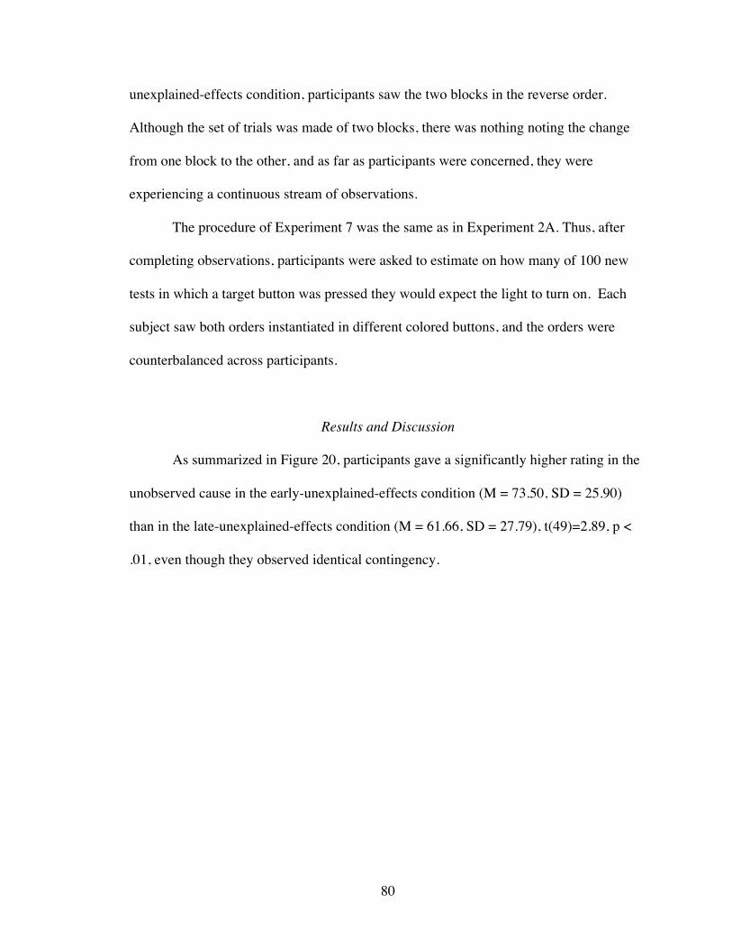
80

unexplained-effects condition, participants saw the two blocks in the reverse order.

Although the set of trials was made of two blocks, there was nothing noting the change

from one block to the other, and as far as participants were concerned, they were

experiencing a continuous stream of observations.

The procedure of Experiment 7 was the same as in Experiment 2A. Thus, after

completing observations, participants were asked to estimate on how many of 100 new

tests in which a target button was pressed they would expect the light to turn on. Each

subject saw both orders instantiated in different colored buttons, and the orders were

counterbalanced across participants.


As summarized in Figure 20, participants gave a significantly higher rating in the

unobserved cause in the early-unexplained-effects condition (M = 73.50, SD = 25.90)

than in the late-unexplained-effects condition (M = 61.66, SD = 27.79), t(49)=2.89, p <

.01, even though they observed identical contingency.

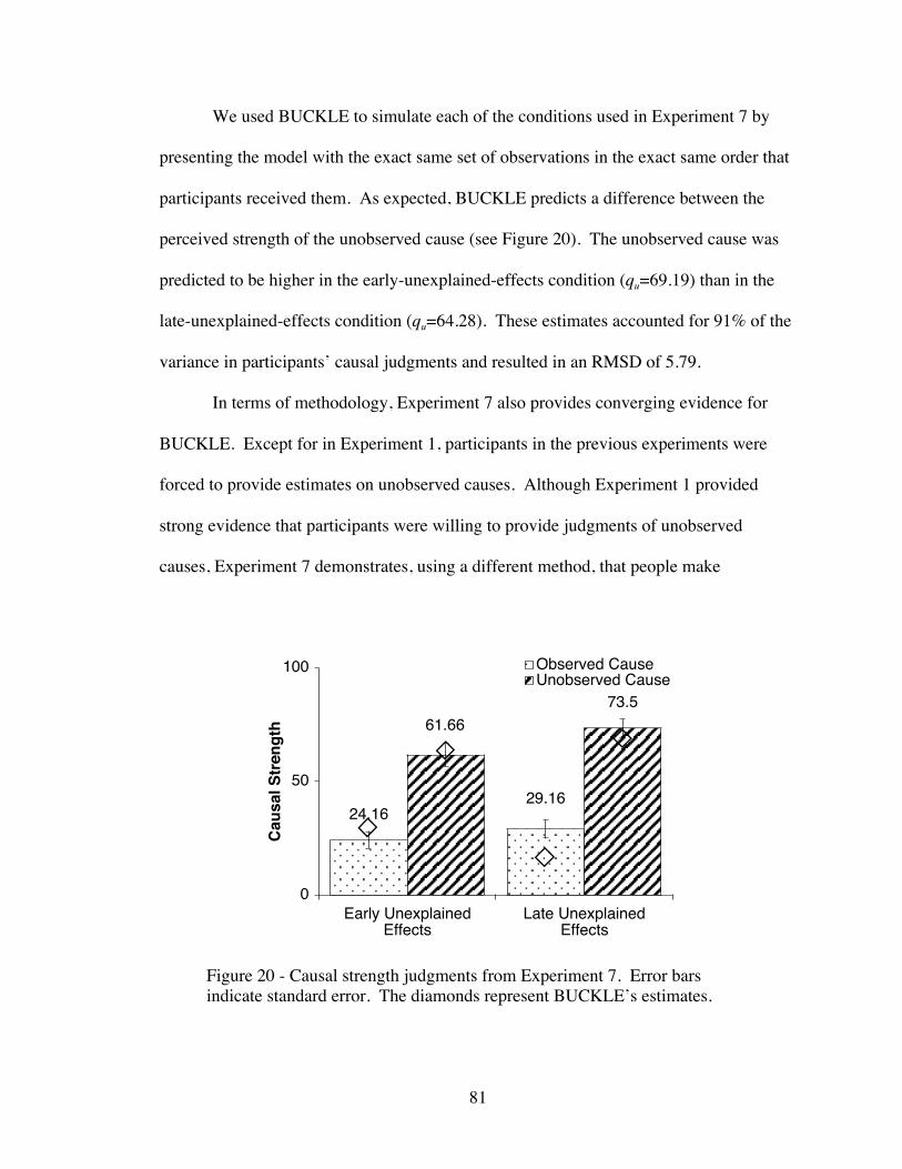
81

We used BUCKLE to simulate each of the conditions used in Experiment 7 by

presenting the model with the exact same set of observations in the exact same order that

participants received them. As expected, BUCKLE predicts a difference between the

perceived strength of the unobserved cause (see Figure 20). The unobserved cause was

predicted to be higher in the early-unexplained-effects condition (qu=69.19) than in the

late-unexplained-effects condition (qu=64.28). These estimates accounted for 91% of the

variance in participants’ causal judgments and resulted in an RMSD of 5.79.

In terms of methodology, Experiment 7 also provides converging evidence for

BUCKLE. Except for in Experiment 1, participants in the previous experiments were

forced to provide estimates on unobserved causes. Although Experiment 1 provided

strong evidence that participants were willing to provide judgments of unobserved

causes, Experiment 7 demonstrates, using a different method, that people make

Figure 20 - Causal strength judgments from Experiment 7. Error barsindicate standard error. The diamonds represent BUCKLE’s estimates.

29.1624.16

61.6673.5

0

50

100

Early UnexplainedEffects

Late UnexplainedEffects

Caus

al S

treng

th


82

spontaneous inferences about unobserved causes. That is, the results from Experiment 7

imply that people spontaneously made inferences about the unobserved cause during the

first block even when they were not prompted to make such judgments. These covert

judgments (e.g., beliefs) then influenced their interpretations of later observations,

resulting in the order effect.

Experiment 8: The Influence of

€

OE Observations

As demonstrated so far,

€

OE observations (or unexplained effects) act to increase

the perceived strength of the unobserved cause, because

€

OE observations necessarily

imply that the unobserved cause has caused the effect on that occasion. One might

suppose that

€

OE observations would act in the opposite manner. When encountering an

€

OE observation, the learner might conclude that the unobserved cause prevented the

effect. Such an interpretation should act to decrease the perceived strength of the

unobserved cause.

According to BUCKLE, this is not necessarily the case for the following reason.

Assuming that o is generative and u is preventative, the likelihood computations used by

BUCKLE assume that

€

OE observations occur for two separate reasons (see Equation

A11 in Appendix A). First, as just mentioned,

€

OE observations could occur when the

effect is prevented from occurring by a preventative unobserved cause. Second,

€

OE

observations could occur because the observed cause itself is not entirely sufficient to

bring about the effect. This latter interpretation should leave the state (i.e., present vs.

absent) of the unobserved cause relatively ambiguous and thus reduce the amount of

learning taking place during

€

OE observations.

83

The suggestion that

€

OE observations do not necessarily lead to the perception of

a preventative unobserved cause has already been supported by the results of Experiment

2. Though the Insufficient condition included

€

OE observations, our participants judged

the unobserved cause to be somewhat generative (M = 27.25, SD = 35.56 in Experiment

2A) rather than preventative. However, BUCKLE predicts that, if it were established that

the observed cause was sufficiently strong cause, then

€

OE observations should indicate

the influence of a preventive unobserved cause. More specifically, the term,

€

P(o)• (1− qo)• 1− P(u |o)[ ]{ }, from the denominator of Equation A11 in Appendix A will

decrease, and increase the likelihood of the unobserved cause being present. Because the

unobserved cause is likely present in the absence of the effect, qu will decrease (i.e., it

will become a stronger preventative cause; see the simulations below).

To test this prediction, Experiment 8 utilized two phases of training. During the

first phase, participants learned that the observed cause was a strong cause of the effect.

In the second phase, participants were exposed to

€

OE observations. According to

BUCKLE, the first phase should decrease the likelihood that the observed cause was

insufficient to bring about the effect and increase the likelihood that the unobserved cause

exerted a preventative influence in the second phase. Thus, this paradigm should allow

€

OE result in preventative judgments of the unobserved cause.

This prediction is consistent with the results from Schulz et al. (2005) discussed

earlier in the introduction. To reiterate, they found that preschoolers perceived an

unobserved cause as preventative after encountering

€

OE observations. Schulz et al.

argued that this occurs because preschoolers believe that whenever a cause is present, an

effect must occur. Under this belief, the only way

€

OE could be possible is when there is

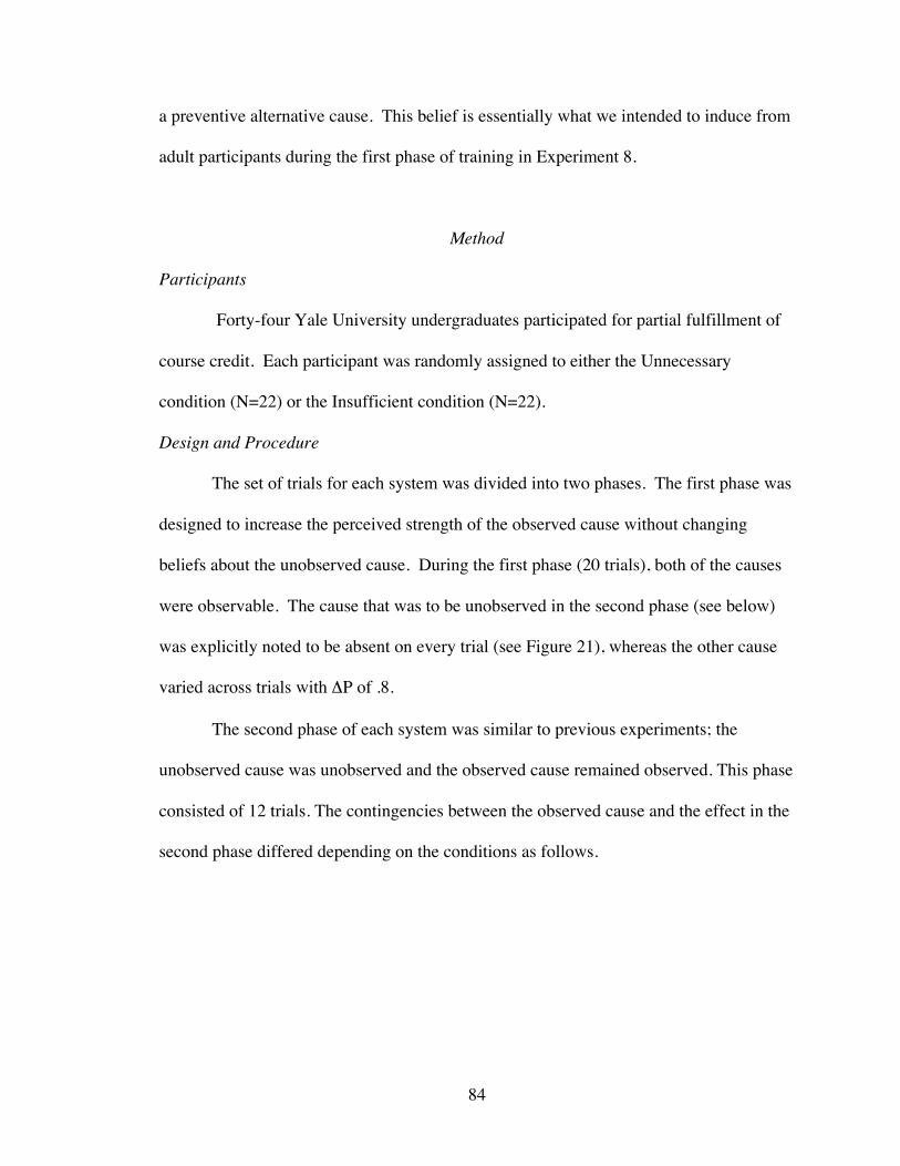
84

a preventive alternative cause. This belief is essentially what we intended to induce from

adult participants during the first phase of training in Experiment 8.

Method

Participants

Forty-four Yale University undergraduates participated for partial fulfillment of

course credit. Each participant was randomly assigned to either the Unnecessary

condition (N=22) or the Insufficient condition (N=22).

Design and Procedure

The set of trials for each system was divided into two phases. The first phase was

designed to increase the perceived strength of the observed cause without changing

beliefs about the unobserved cause. During the first phase (20 trials), both of the causes

were observable. The cause that was to be unobserved in the second phase (see below)

was explicitly noted to be absent on every trial (see Figure 21), whereas the other cause

varied across trials with ΔP of .8.

The second phase of each system was similar to previous experiments; the

unobserved cause was unobserved and the observed cause remained observed. This phase

consisted of 12 trials. The contingencies between the observed cause and the effect in the

second phase differed depending on the conditions as follows.

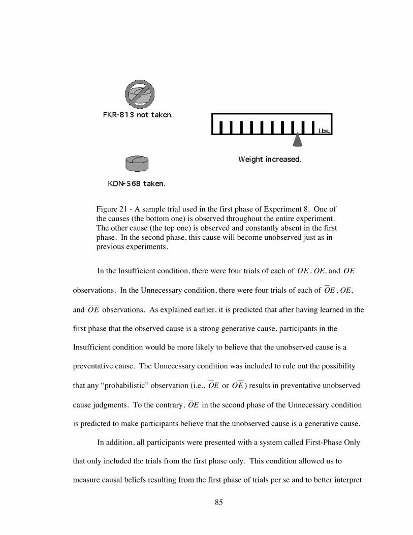
85

In the Insufficient condition, there were four trials of each of

€

OE , OE, and

€

OE

observations. In the Unnecessary condition, there were four trials of each of

€

OE , OE,

and

€

OE observations. As explained earlier, it is predicted that after having learned in the

first phase that the observed cause is a strong generative cause, participants in the

Insufficient condition would be more likely to believe that the unobserved cause is a

preventative cause. The Unnecessary condition was included to rule out the possibility

that any “probabilistic” observation (i.e.,

€

OE or

€

OE ) results in preventative unobserved

cause judgments. To the contrary,

€

OE in the second phase of the Unnecessary condition

is predicted to make participants believe that the unobserved cause is a generative cause.

In addition, all participants were presented with a system called First-Phase Only

that only included the trials from the first phase only. This condition allowed us to

measure causal beliefs resulting from the first phase of trials per se and to better interpret

Figure 21 - A sample trial used in the first phase of Experiment 8. One ofthe causes (the bottom one) is observed throughout the entire experiment.The other cause (the top one) is observed and constantly absent in the firstphase. In the second phase, this cause will become unobserved just as inprevious experiments.

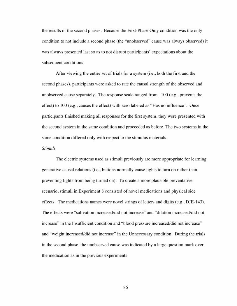
86

the results of the second phases. Because the First-Phase Only condition was the only

condition to not include a second phase (the “unobserved” cause was always observed) it

was always presented last so as to not disrupt participants’ expectations about the

subsequent conditions.

After viewing the entire set of trials for a system (i.e., both the first and the

second phases), participants were asked to rate the causal strength of the observed and

unobserved cause separately. The response scale ranged from –100 (e.g., prevents the

effect) to 100 (e.g., causes the effect) with zero labeled as “Has no influence”. Once

participants finished making all responses for the first system, they were presented with

the second system in the same condition and proceeded as before. The two systems in the

same condition differed only with respect to the stimulus materials.

Stimuli

The electric systems used as stimuli previously are more appropriate for learning

generative causal relations (i.e., buttons normally cause lights to turn on rather than

preventing lights from being turned on). To create a more plausible preventative

scenario, stimuli in Experiment 8 consisted of novel medications and physical side

effects. The medications names were novel strings of letters and digits (e.g., DJE-143).

The effects were “salivation increased/did not increase” and “dilation increased/did not

increase” in the Insufficient condition and “blood pressure increased/did not increase”

and “weight increased/did not increase” in the Unnecessary condition. During the trials

in the second phase, the unobserved cause was indicated by a large question mark over

the medication as in the previous experiments.

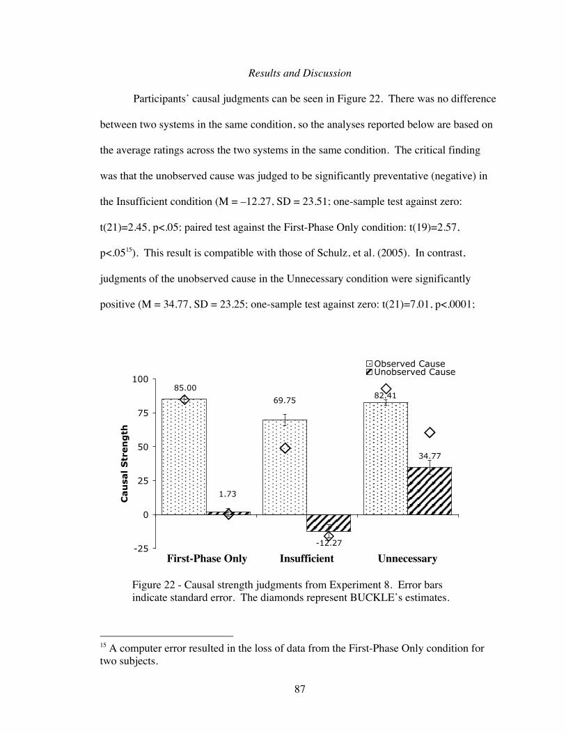
87


Participants’ causal judgments can be seen in Figure 22. There was no difference

between two systems in the same condition, so the analyses reported below are based on

the average ratings across the two systems in the same condition. The critical finding

was that the unobserved cause was judged to be significantly preventative (negative) in

the Insufficient condition (M = –12.27, SD = 23.51; one-sample test against zero:

t(21)=2.45, p<.05; paired test against the First-Phase Only condition: t(19)=2.57,

p<.0515). This result is compatible with those of Schulz, et al. (2005). In contrast,

judgments of the unobserved cause in the Unnecessary condition were significantly

positive (M = 34.77, SD = 23.25; one-sample test against zero: t(21)=7.01, p<.0001;

15 A computer error resulted in the loss of data from the First-Phase Only condition fortwo subjects.

Figure 22 - Causal strength judgments from Experiment 8. Error barsindicate standard error. The diamonds represent BUCKLE’s estimates.

82.4169.75

85.00

-12.27

34.77

1.73

-25

0

25

50

75

100

Cau

sal

Str

en

gth


UnnecessaryInsufficientFirst-Phase Only

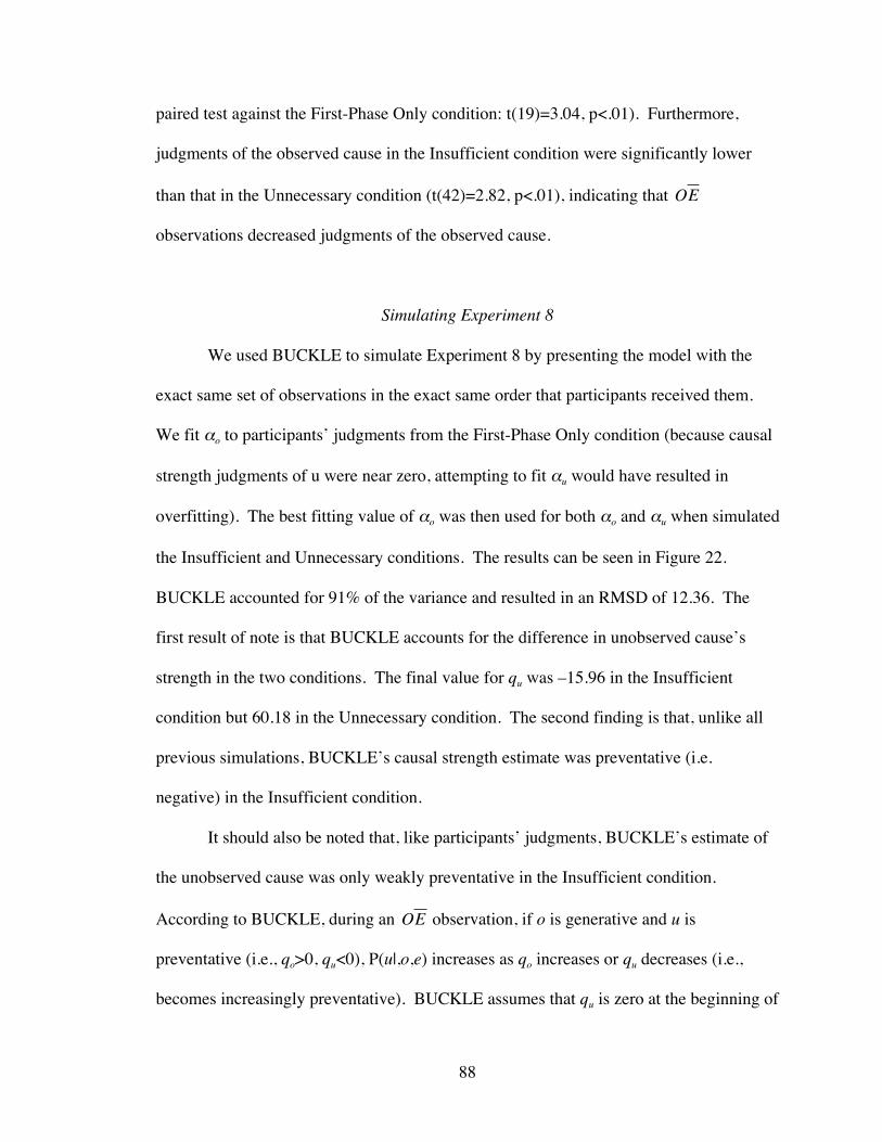
88

paired test against the First-Phase Only condition: t(19)=3.04, p<.01). Furthermore,

judgments of the observed cause in the Insufficient condition were significantly lower

than that in the Unnecessary condition (t(42)=2.82, p<.01), indicating that

€

OE

observations decreased judgments of the observed cause.

Simulating Experiment 8

We used BUCKLE to simulate Experiment 8 by presenting the model with the

exact same set of observations in the exact same order that participants received them.

We fit αo to participants’ judgments from the First-Phase Only condition (because causal

strength judgments of u were near zero, attempting to fit αu would have resulted in

overfitting). The best fitting value of αo was then used for both αo and αu when simulated

the Insufficient and Unnecessary conditions. The results can be seen in Figure 22.

BUCKLE accounted for 91% of the variance and resulted in an RMSD of 12.36. The

first result of note is that BUCKLE accounts for the difference in unobserved cause’s

strength in the two conditions. The final value for qu was –15.96 in the Insufficient

condition but 60.18 in the Unnecessary condition. The second finding is that, unlike all

previous simulations, BUCKLE’s causal strength estimate was preventative (i.e.

negative) in the Insufficient condition.

It should also be noted that, like participants’ judgments, BUCKLE’s estimate of

the unobserved cause was only weakly preventative in the Insufficient condition.

According to BUCKLE, during an

€

OE observation, if o is generative and u is

preventative (i.e., qo>0, qu<0), P(u|,o,e) increases as qo increases or qu decreases (i.e.,

becomes increasingly preventative). BUCKLE assumes that qu is zero at the beginning of

89

Experiment 8’s second phase and thus qu does not act to substantially increase the

likelihood of u. However, qo should be high at the beginning of the second phase.

Shouldn’t this increase the likelihood of u (and thus decrease qu)? According to

BUCKLE’s likelihood computation (see Appendix A), even when qu is small (e.g., -.01),

and qo is large (e.g., 0.9), the likelihood of u will be only slightly greater than chance

(e.g., .52). It is only when the perceived strength of the observed cause is near maximal

that

€

OE observations will lead to large negative values of qu (e.g., when qo=0.999 and

qu=-.01, the likelihood of u is .92). Thus, BUCKLE intuitively suggests that the strength

of the observed cause will predict the magnitude of the influence of

€

OE observations on

unobserved cause judgments.

Thus, according to BUCKLE, even when the observed cause is reasonably strong,

€

OE observations remain somewhat ambiguous. Because of this, even in the Insufficient

condition BUCKLE allows the possibility that the observed cause was insufficient to

bring about the effect. This interpretation causes BUCKLE to decrease the perceived

strength of the observed cause. Thus, just as was found in the current study, BUCKLE

argues that the observed cause in the Insufficient condition (qu = 49.05) should be

perceived as weaker than in the Unnecessary condition (qu =93.04; see Figure 22).

Summary

Experiment 8 illustrated that

€

OE observations do not necessarily lead learners to

perceive the unobserved cause as preventative. BUCKLE argues that this is because

€

OE

observations have ambiguous implications for unobserved causes. The current

experiment included a pre-training phase designed to minimize this ambiguity. As

90

predicted, with the pre-training, participants were able to use

€

OE observations to infer a

preventative influence of an unobserved cause. In addition, BUCKLE mirrored more

subtle elements of participants’ behavior. The

€

OE observations led to small decreases in

the perceived strength of the observed cause. Perhaps more surprising is the fact that

€

OE

observations led to only weakly preventative causal judgments. BUCKLE argues that

this again occurs because of the ambiguity inherent in

€

OE observations. Only when the

observed cause is near-absolutely sufficient (perhaps as in the beliefs of preschoolers,

Schulz, et al., 2005) will the unobserved cause be perceived as strongly preventative.

91

CHAPTER VI

GENERAL DISCUSSION

The model proposed here, BUCKLE, describes a simple two-step process for

learning in the presence of unobserved causes. Each of the two steps involves a

probabilistic inference about the likelihood of an event occurring. Each of these steps

occurs on every learning occasion and together allows causal beliefs to be modified over

the course of learning. The first step is to compute how likely the unobserved cause is to

be present. This inference is made using both information available in the environment

(e.g., the state of observed causes and effects), as well as beliefs and assumptions (e.g.,

the belief about the current strength of the observed cause). After this inference is made,

there is no longer any missing information; all causes are believed to be present with

some likelihood. The second step is to learn about the underlying casual relationships.

To do this, BUCKLE makes a prediction about how likely the effect is to be present

given the currently available information (e.g., the state of observed and unobserved

causes and effects and beliefs and assumptions). This inference allows BUCKLE to

compare its beliefs about how the world operates (i.e., the likelihood inference) with the

actual operation of the world (i.e., whether the effect actually occurred or not). Errors in

this step’s inference then form the basis of learning. Despite its relative simplicity,

BUCKLE appears to accurately capture a significant variety of aspects of people’s cause

learning.

92

Given a variety of statistical environments, BUCKLE successfully accounted for

participants’ causal strength judgments. In particular, BUCKLE anticipated the

substantial influence of unexplained effects (

€

OE observations) on judgments of the

unobserved cause, which in turn influenced judgments of the observed cause. BUCKLE

also accounted for more subtle behavior. For example, when participants encountered

€

OE observations, they did not necessarily judge the unobserved cause to be preventative.

This finding is contrary to the predictions of several models and appears to contradict

previously reported findings in children (Schulz, et al., 2005). However, given the details

of BUCKLE’s operation, we were able to speculate about why our result was obtained

and what the underlying developmental difference might have been. This allowed us to

design a situation that elicited preventative judgments, providing further evidence in

support of BUCKLE’s account and eliminating the apparent contradiction.

The ability to predict causal strength judgments is an obvious first requirement for

any model of causal learning. Indeed, fits to such judgments have been the primary

method of validating causal learning models (e.g., Buehner, et al. 2003; Lober & Shanks,

2000). Of course, the point of modeling any psychological process is to allow a deeper

understanding of its operation. Fortunately, BUCKLE details a rich process that can be

investigated in its own right. The most obvious byproduct of BUCKLE’s process is the

result from BUCKLE’s first step: the inference about the likelihood of the unobserved

cause. Again, using a variety of situations, our participants’ estimates consistently

mirrored those of BUCKLE on several different dimensions. For example, likelihood

estimates were greatly influenced by the state of the observed cause and effect. However,

as predicted by BUCKLE, even identical observations elicited reliably different

93

likelihood judgments under appropriate circumstances. This insight allowed us to

produce what may be the most dramatic illustration of BUCKLE’s process-oriented

nature. While presenting participants with identical sets of trials, we were able to elicit

predictably different causal strength judgments.

The Interchangeable Nature of BUCKLE

As with any model, there are many assumptions built into BUCKLE. Some of

these assumptions are captured by the values of various unchanging parameters (see

Table A1). However there are other, less obvious assumptions behind BUCKLE’s

operation demonstrated in this paper. For example, BUCKLE, as described so far,

assumes that each cause has an independent influence on its effect. Such an assumption

disallows causal interactivity that is often (if not always) present in the real world. For

example, individually, gasoline and key-turning do not cause your car to start; both

causes are needed together before the effect will occur.

Independent influence and causal interactivity describe qualitatively different

ways in which causes may operate. In the language of causal maps (see Pearl, 2000 for a

thorough review), this is a difference in parameterization. Independence and interactivity

are only two possible parameterizations. In theory, there are an infinite number of

parameterizations for any given set of causes and effects.

Fortunately, different parameterizations are easy to implement in BUCKLE. For

example, given the assumption that causes exert independent influence on their effects,

the expressions described in Appendix A and Equations 2-7 are appropriate to compute

the desired likelihood. However, if causes do not exert independent influence on their

94

effects, different expressions are needed to compute the same likelihood. Take the

example of computing the likelihood of the unobserved cause (BUCKLE’s first step).

Equation 1 can still be used, coupled with a specification of the different ways in which

each type of observation can occur and their associated probabilities. This information is

precisely what is described by a given parameterization. Thus, if BUCKLE were used to

simulate learning in a domain where causal interactivity were assumed, the expressions

used to elaborate Equation 1 (i.e., Appendix A) would need to be rewritten to reflect the

change in parameterization. The same is true of BUCKLE’s second step. Equations 2-7

provide the appropriate way to compute the likelihood of the effect under a noisy-

OR/noisy-AND-NOT parameterization. However, if it were discovered that a different

parameterization better described people’s beliefs, the relevant expressions could be

substituted.

Causal interactivity is not the only alternative parameterization that is

psychologically plausible. Recent work by Beckers and colleagues (Beckers, De

Houwer, Pineno, & Miller, 2005; Beckers, Miller, De Houwer, & Urushihara, in press;

see also Griffiths & Tenenbaum, 2005) has shed light on the inferences that are only

allowable when the effect is a continuous variable (e.g., temperature). BUCKLE, as

described here, assumes that effects (all events actually) are discrete. Clearly entirely

different parameterizations are required when dealing with continuous effects. In such a

situation, the likelihood of the effect is a distribution (or distributions) over possible

values of the effect rather than single probabilities. In particular, Beckers argues that

people generally assume that multiple effective causes lead to a stronger effect than a

single effective cause. This assumption implies a particular class of parameterizations

95

and, again, such parameterizations would imply a different set of expressions for the

inferences prescribed by BUCKLE.

Note that BUCKLE is not alone in this flexibility. Any model that explicitly

adopts a causal parameterization (e.g., MLE; Tenenbaum & Griffiths, 2005) will need to

change its specific computations if the parameterization changes. As causal models have

gained in popularity, more models are explicitly acknowledging their parameterization

assumptions. What these models share is a commitment to describe inferences that are

specifically causal. This means that the assumptions about causality are explicit in their

computation. The same cannot be said for non-causal models of learning such as the

constraint-satisfaction and RW models. For example, it is unclear why RW uses the sum

of associative strengths as the basis of its error-correction algorithm16. However, the

reason for this choice certainly does not have anything to do with how causes behave,

because RW is claimed to be a general (i.e., non-causal) model of learning. Thus, models

such as RW cannot be adapted to deal with different, specifically causal, assumptions.

This rigidity formed the basis of Waldmann’s (1996, 2000, 2001) studies as well as our

own Experiment 6. Thus, unlike BUCKLE, these non-causal models have no way of

predicting, a priori, that beliefs about parameterization should influence causal learning.

In this section, we have discussed various ways in which BUCKLE can be

extended. Of course, arbitrary changes to BUCKLE could lead to an ultimately

unfalsifiable model. Instead, we have attempted to illustrate that there is a principled

16 “The associative strength of the compound, VAX, must somehow be specified in terms ofthe strengths of the components. The simplest assumption, and the one we will makehere, is VAX = VA + VX,” (Rescorla & Wagner, 1972). Of course, if RW is treated as amodel of causal learning, then its assumptions about parameterization may be revealed(Tenenbaum & Griffiths, 2005). However, as its advocates claim (Shanks, et al., 1996),RW is not a model of causal learning.

96

relationship between assumptions about particular learning environments and the details

of BUCKLE’s operation. To reiterate the core principles, BUCKLE predicts that learners

typically represent an unobserved cause and learn about it using a two-step process. The

first step is to infer the likelihood that the unobserved cause is present. Using the result

of this inference, the strength of all causes, observed and unobserved, is adjusted.

Similarity between BUCKLE and Other Models of Learning

As briefly mentioned in the introduction, BUCKLE shares theoretical foundations

with several existing models. The idea of error-correction learning has a long history in

the psychology of learning (e.g., Widrow & Hoff, 1960). In particular, Rescorla and

Wagner (1972) used error-correction to model behavior (as opposed to neural activity).

The success of RW in accounting for learning behavior has led to its continued use even

more than thirty years later. Of course, as just discussed, we believe that RW has

features that limit its ability to account for a variety of causal learning phenomena.

To remedy these limitations, BUCKLE uses a slightly different model of causal

learning based on suggestions of Danks, et al. (2003). This model has two related

features that set it apart form RW. First, as just discussed, Danks, et al. (2003) method

uses a noisy-OR parameterization to compute the likelihood of the effect. BUCKLE

elaborates this by using either a noisy-OR parameterization when dealing with generative

causes and a noisy-AND-NOT parameterization when one cause is preventative. This

has two advantages. First, recent work (Cheng, 1997; Novick & Cheng, 2004; Griffiths

& Tenenbaum, 2005; Danks, Griffiths, & Tenenbaum, 2003; Steyvers, Tenenbaum,

Wagenmakers, & Blum, 2003) suggests that the noisy-OR/AND-NOT parameterization

97

better describes people’s causal beliefs. Second, and perhaps more critically, building a

model around the explicit notion of parameterization allows flexibility otherwise

unthinkable. If noisy-OR/AND-NOT parameterizations only work in certain domains of

causality, the model can simply be changed based on the new assumptions.

The second, related difference between RW and the proposal of Danks, et al.

(2003) has to do with the quantity being computed. RW computes associative strength, a

quantity that has been related to measurements of learning, but who’s exact meaning is

unclear. Associative strength is often related to, “magnitude or probability of conditioned

responding” (Rescorla & Wagner, 1972) in conditioning experiments. In human causal

learning studies, associative strength has been mapped onto a scale that includes

preventative cause (negative associative strengths), ineffective causes (associative

strengths of zero), and generative cause (negative associative strengths). Associative

strength also tends to capture both aspects of a cause’s sufficiency and its necessity (see

Cheng, 1997 for details on the relationship between ΔP and RW). BUCKLE and the

model of Danks, et al. (2003) do not learn associative strength. Instead, they learn a

quantity that describes a cause’s sufficiency. As mentioned in the introduction, this

quantity is essentially what Pearl (2000) calls PS and what Cheng (2000) calls contextual

causal power. The reason we chose this quantity actually has more to do with

methodological cleanliness than any deep theoretical motivation. When eliciting

judgments of associative strength, a vague question about “the degree to which A causes

B” has traditionally been used (e.g., Wasserman, Kao, Van Hamme, Katagiri & Young,

1996). Recent work (Griffiths & Tennenbaum, 2005; White, 1992) has noted that the

ambiguity of this question could elicit several, qualitatively different quantities. To elicit

98

the quantity computed by BUCKLE, a more concrete question is required, and thus we

can be more assured that our participants’ judgments reflect the quantity of interest.

The models discussed so far have all been related to BUCKLE’s learning process

(the second step) and not the first, inference step. More broadly, the idea of combining

the two steps (filling in missing data and learning) has a long history in the field of

machine learning. For example, Dempster, Laird, and Rubin (1977) describe an

algorithm called EM (see also McLachlan and Krishnan, 1997; Tanner, 1996) that is able

to successfully estimate parameters even when there are missing data. Like BUCKLE,

EM consists of two, repeated steps. The first step (the E step) is to compute a likelihood

distribution over possible values of the missing data. In the current studies, this step

would compute the likelihood that the unobserved cause was present or absent on all

trials. This step essentially acts to “fill in” missing data. The second step (the M step) is

to find the set of parameters that maximizes the distribution computed in the first step. In

the current studies, this would be equivalent to computing the MLE of qu and qo given the

observed data as well as the data inferred in the first step. These two steps are repeated

until parameter estimates converge. EM has been shown to successfully converge on

locally maximal parameter estimates (Dempster, Laird, and Rubin, 1977 provided the

proof).

Though BUCKLE and EM share a conceptual approach to the problem of missing

data, there are several differences. The largest difference is that EM performs its two

steps over the entire dataset simultaneously whereas BUCKLE performs its two steps on

one observation at a time. As a result, EM cannot begin learning until all the data are

collected. Thus, EM describes an inference that requires multiple iterations before

99

settling (much like the constraint-satisfaction network utilized in the current study)

whereas BUCKLE describes a trial-by-trial learning that allows beliefs to be modified in

a piecemeal fashion. This essentially prohibits EM from dealing with the dynamics of

learning found in several of the current experiments. For example, because EM ignores

trial order, it would not demonstrate the order effects found in Experiment 7.

There have been attempts to modify EM to be incremental (i.e., dealing with one

data item at a time). The motivation for this effort generally comes, not from a desire to

be psychologically plausible, but from a need to find efficient algorithms in the face of

massive datasets (e.g., data mining large databases). For example, Neal and Hinton

(1998) demonstrate that a modified EM algorithm requiring only one data item at a time

is equivalent to the canonical version of EM and is thus guaranteed to converge in the

same manner (though faster). However, even this incremental variant was designed to be

run on a complete dataset. For example, Neal and Hinton (1998) state that, “data items

might be selected for updating in the E step cyclically, or by some scheme that gives

preference to data items for which [the likelihood distribution] has not yet stabilized”.

Thus, the advantage of this algorithm is not in allowing for incremental learning, but in

its ability to learn from complete datasets more efficiently.

Others have suggested EM algorithms that are truly incremental (i.e., require only

one forward pass through the data; Bradley, Fayyad, & Reina, 1998; Suematsu,

Maebashi, Hayashi, 2004). However, these algorithms uniformly require considerable

computation and complex storage (e.g. clustering). BUCKLE is certainly a member of

this family of algorithms. BUCKLE’s certainly two steps mirror those of EM. However,

BUCKLE is also certainly a simplistic variant of EM. The most obvious example of this

100

is the fact that BUCKLE does not maximize its parameter estimates in the second step.

Instead, it uses the more obviously psychologically plausible notion of error-correction.

Nor does BUCKLE labor over the inference of its first step. It simply makes its best

guess given the available information and moves on. These features may no doubt lead

BUCKLE’s behavior to deviate from more complex EM variants, however, future work

is required to more thoroughly explore this speculation.

Conclusion

Knowledge about alternative causes is crucial in inducing causation from

covariation. Previous models of causal learning have acknowledged the importance of

alternative causes but have only made simplified assumptions about learning of

unobserved alternative causes. The current paper presents empirical evidence suggesting

that people willingly make sophisticated inferences about unobserved causes. We have

presented a new model of causal induction that delineates bases of such inferences and

demonstrated that BUCKLE could explain unobserved causal learning better than

existing models. As a result, BUCKLE could explain observed causal learning under

confounded situations better than existing models.

Because the current paper is the first thorough investigation of a model that is

specifically designed to deal with unobserved causal learning, most of our discussion and

experiments were focused on unobserved causal learning. Future research can further

examine other possible consequences of unobserved causal inferences on learning of

observed causes. We have also discussed many ways in which BUCKLE can be flexibly

expanded to accommodate causal environments different from those used in our current

101

experiments. Further research is needed to test the psychological validity of these

extensions.

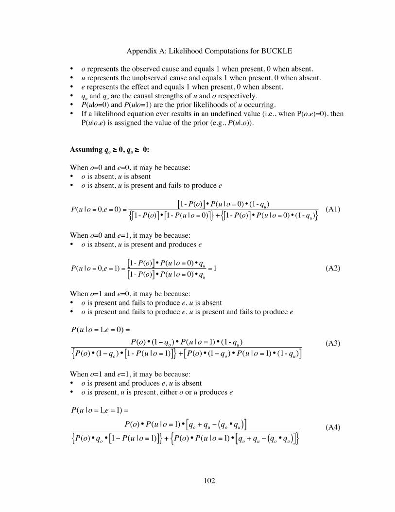
102

Appendix A: Likelihood Computations for BUCKLE

• o represents the observed cause and equals 1 when present, 0 when absent.• u represents the unobserved cause and equals 1 when present, 0 when absent.• e represents the effect and equals 1 when present, 0 when absent.• qu and qo are the causal strengths of u and o respectively.• P(u|o=0) and P(u|o=1) are the prior likelihoods of u occurring.• If a likelihood equation ever results in an undefined value (i.e., when P(o,e)=0), then

P(u|o,e) is assigned the value of the prior (e.g., P(u|,o)).

Assuming qo ≥ 0, qu ≥ 0:

When o=0 and e=0, it may be because:• o is absent, u is absent• o is absent, u is present and fails to produce e

€

P(u |o = 0,e = 0) =1- P(o)[ ] •P(u |o = 0)• (1- qu)

1- P(o)[ ] • 1- P(u |o = 0)[ ]{ } + 1- P(o)[ ] •P(u |o = 0)• (1- qu){ }(A1)

When o=0 and e=1, it may be because:• o is absent, u is present and produces e

€

P(u |o = 0,e =1) =1- P(o)[ ] •P(u |o = 0)•qu1- P(o)[ ] •P(u |o = 0)•qu

=1 (A2)

When o=1 and e=0, it may be because:• o is present and fails to produce e, u is absent• o is present and fails to produce e, u is present and fails to produce e

€

P(u |o =1,e = 0) =

P(o)• (1− qo)•P(u |o =1)• (1- qu)P(o)• (1− qo)• 1- P(u |o =1)[ ]{ } + P(o)• (1− qo)•P(u |o =1)• (1- qu)[ ]

(A3)

When o=1 and e=1, it may be because:• o is present and produces e, u is absent• o is present, u is present, either o or u produces e

€

P(u |o =1,e =1) =

P(o)•P(u |o =1)• qo + qu − qo •qu( )[ ]P(o)•qo • 1− P(u |o =1)[ ]{ } + P(o)•P(u |o =1)• qo + qu − qo •qu( )[ ]{ }

(A4)

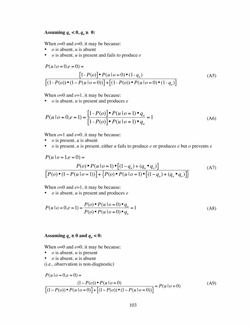
103

Assuming qo < 0, qu ≥ 0:

When o=0 and e=0, it may be because:• o is absent, u is absent• o is absent, u is present and fails to produce e

€

P(u |o = 0,e = 0) =

1- P(o)[ ] •P(u |o = 0)• (1- qu)(1- P(o))• (1− P(u |o = 0))[ ] + (1- P(o))•P(u |o = 0)• (1- qu)[ ]

(A5)


€

P(u |o = 0,e =1) =1- P(o)[ ] •P(u |o =1)•qu1- P(o)[ ] •P(u |o =1)•qu

=1 (A6)

When o=1 and e=0, it may be because:• o is present, u is absent• o is present, u is present, either u fails to produce e or produces e but o prevents e

€

P(u |o =1,e = 0) =

P(o)•P(u |o =1)• (1− qu) + (qu •qo)[ ]P(o)• (1− P(u |o =1))[ ] + P(o)•P(u |o =1)• (1− qu) + (qu •qo)[ ]{ }

(A7)


€

P(u |o = 0,e =1) =P(o)•P(u |o = 0)•quP(o)•P(u |o = 0)•qu

=1 (A8)

Assuming qo ≥ 0 and qu < 0:

When o=0 and e=0, it may be because:• o is absent, u is present• o is absent, u is absent(i.e., observation is non-diagnostic)

€

P(u |o = 0,e = 0) =

(1− P(o))•P(u |o = 0)(1− P(o))•P(u |o = 0)[ ] + (1− P(o))• (1− P(u |o = 0))[ ]

= P(u |o = 0) (A9)

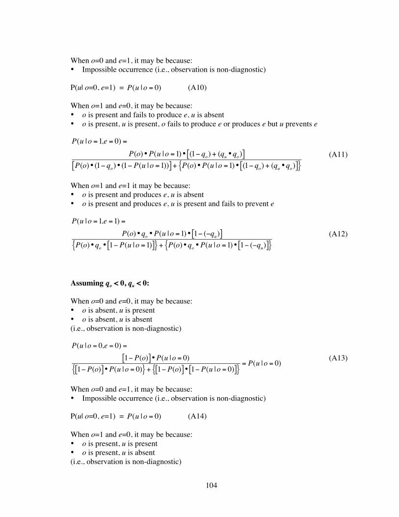
104

When o=0 and e=1, it may be because:• Impossible occurrence (i.e., observation is non-diagnostic)

P(u| o=0, e=1) =

€

P(u |o = 0) (A10)

When o=1 and e=0, it may be because:• o is present and fails to produce e, u is absent• o is present, u is present, o fails to produce e or produces e but u prevents e

€

P(u |o =1,e = 0) =

P(o)•P(u |o =1)• (1− qo) + (qu •qo)[ ]P(o)• (1− qo)• (1− P(u |o =1))[ ] + P(o)•P(u |o =1)• (1− qo) + (qu •qo)[ ]{ }

(A11)

When o=1 and e=1 it may be because:• o is present and produces e, u is absent• o is present and produces e, u is present and fails to prevent e

€

P(u |o =1,e =1) =

P(o)•qo •P(u |o =1)• 1− (−qu)[ ]P(o)•qo • 1− P(u |o =1)[ ]{ } + P(o)•qo •P(u |o =1)• 1− (−qu)[ ]{ }

(A12)

Assuming qo < 0, qu < 0:

When o=0 and e=0, it may be because:• o is absent, u is present• o is absent, u is absent(i.e., observation is non-diagnostic)

€

P(u |o = 0,e = 0) =

1− P(o)[ ] •P(u |o = 0)1− P(o)[ ] •P(u |o = 0){ } + 1− P(o)[ ] • 1− P(u |o = 0)[ ]{ }

= P(u |o = 0) (A13)


P(u| o=0, e=1) =

€

P(u |o = 0) (A14)

When o=1 and e=0, it may be because:• o is present, u is present• o is present, u is absent(i.e., observation is non-diagnostic)

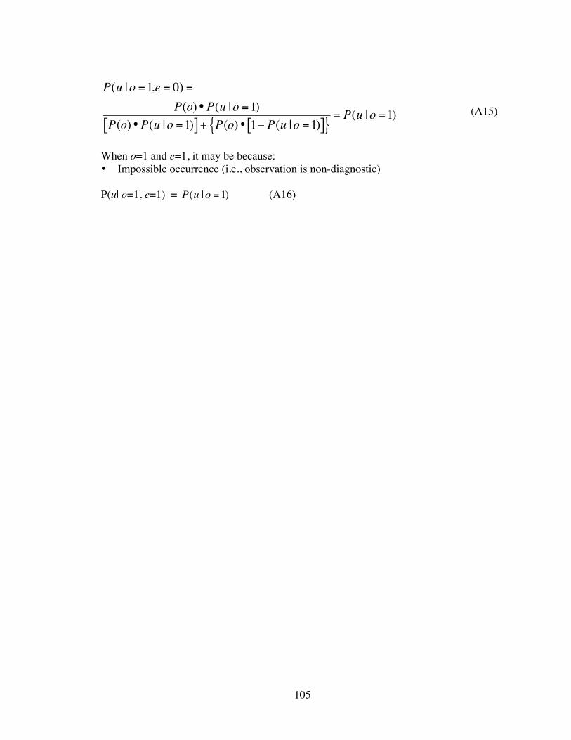
105

€

P(u |o =1,e = 0) =

P(o)•P(u |o =1)P(o)•P(u |o =1)[ ] + P(o)• 1− P(u |o =1)[ ]{ }

= P(u |o =1) (A15)


P(u| o=1, e=1) =

€

P(u |o =1) (A16)

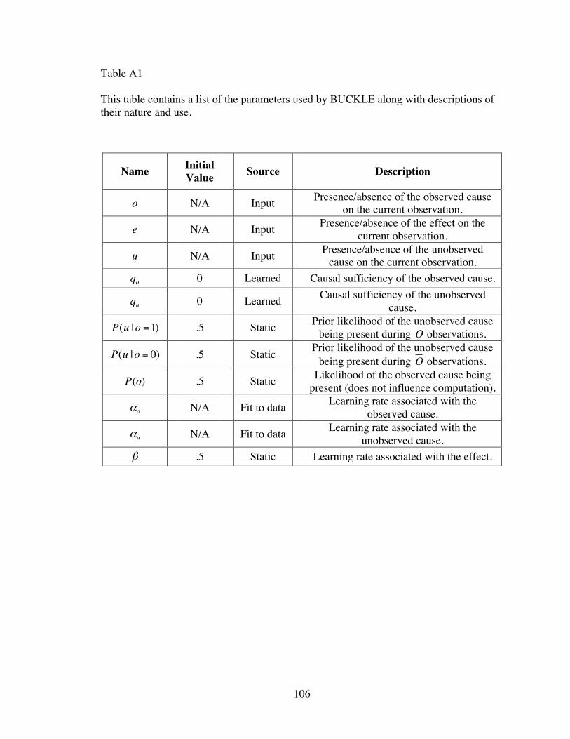
106

Table A1

This table contains a list of the parameters used by BUCKLE along with descriptions oftheir nature and use.

Name InitialValue Source Description

o N/A Input Presence/absence of the observed causeon the current observation.

e N/A Input Presence/absence of the effect on thecurrent observation.

u N/A Input Presence/absence of the unobservedcause on the current observation.

qo 0 Learned Causal sufficiency of the observed cause.

qu 0 Learned Causal sufficiency of the unobservedcause.

€

P(u |o =1) .5 Static Prior likelihood of the unobserved causebeing present during

€

O observations.

€

P(u |o = 0) .5 Static Prior likelihood of the unobserved causebeing present during

€

O observations.

€

P(o) .5 Static Likelihood of the observed cause beingpresent (does not influence computation).

αo N/A Fit to data Learning rate associated with theobserved cause.

αu N/A Fit to data Learning rate associated with theunobserved cause.

β .5 Static Learning rate associated with the effect.

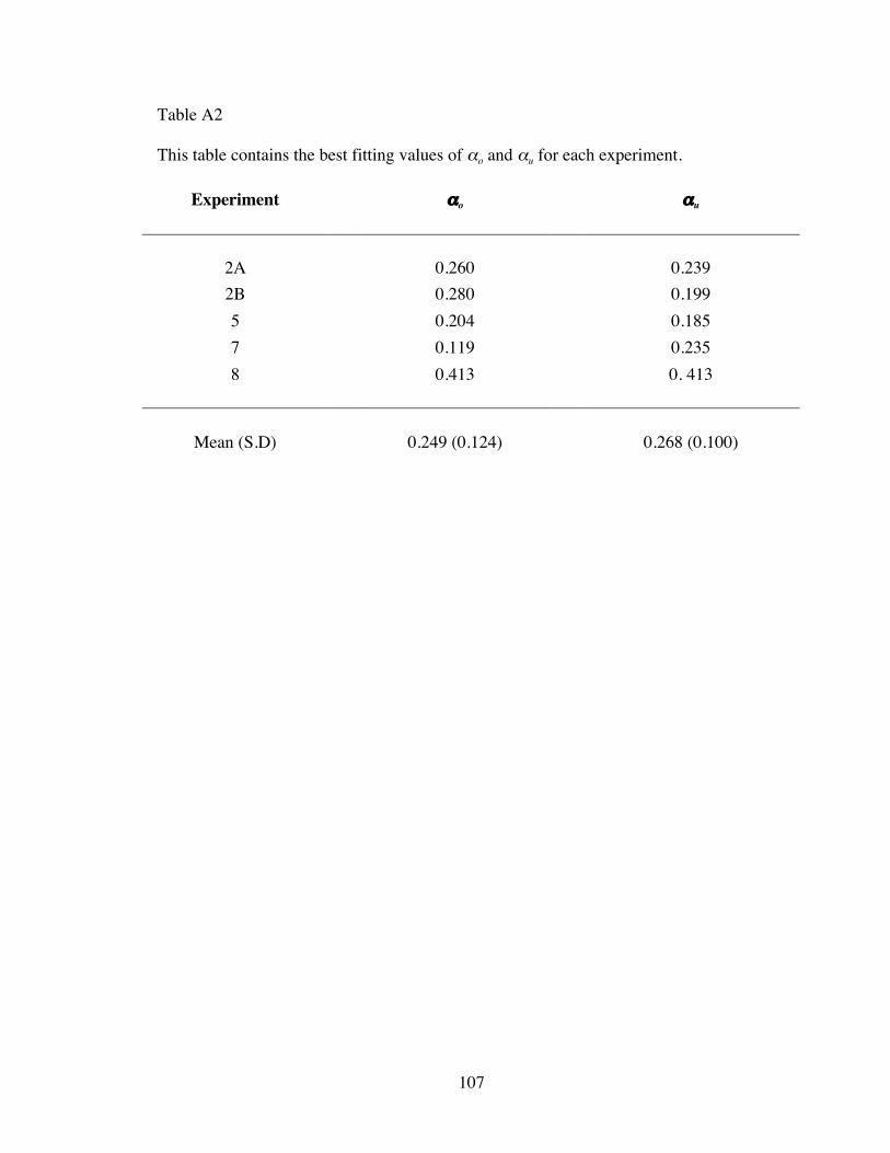
107

Table A2

This table contains the best fitting values of αo and αu for each experiment.

Experiment αo αu

2A 0.260 0.2392B 0.280 0.1995 0.204 0.1857 0.119 0.2358 0.413 0. 413

Mean (S.D) 0.249 (0.124) 0.268 (0.100)

108

Appendix B: Likelihood Computations for MLE

The MLE computes the combination of parameters most likely to have resulted inthe observed data. To do so, we calculate the likelihood of encountering the set ofobservations. If the condition includes the set of observations, D, each containing Nobservations, the likelihood can be computed as follows:

€

L(D |qo,qu) = P(Di |qo,qu)i=1

N

∏ (B1)

The likelihood of all possible combinations of qo and qu can then be computed and thepair that results in the greatest likelihood is the MLE.

To calculate P(Di|qo,qu), we will assume (as we did for BUCKLE) that causescombine in the manner of a noisy-OR/AND-NOT gate. The likelihood of each type ofobservation (i.e., P(Di|qo,qu)) may be computed by combining the likelihood of eachpossible way in which that observation (i.e., Di) could occur (see below). We assumedthat P(u| qo, qu) is a uniform distribution equal to 0.5, indicating complete uncertaintyabout the likelihood of the unobserved cause and that o is independent of u (i.e., P(e|u=1)= P(e|u=0)). As shown in the equation above, by iterating over the observed trial typesand multiplying the individual likelihoods we can compute the overall likelihood of eachpair of parameter values. Doing so for all possible combinations of parameter valuesallows us to find the pair that is most likely given the data.

When o=0 and e=0 it may be because:• o is absent, u is absent• o is absent, u is present and fails to produce e

€

P(o = 0,e = 0 |qo,qu) =

P(o = 0 |qo,qu)• P(u = 0 |qo,qu) + P(u =1 |qo,qu)• (1− qu)[ ]{ }(B2)

When o=0 and e=1 it may be because:• o is absent, u is present and produces e

€

P(o = 0,e =1 |qo,qu) = P(o = 0 |qo,qu)•P(u =1 |qo,qu)•qu (B3)

When o=1 and e=0 it may be because:• o is present and fails to produce e, u is absent• o is present and fails to produce e, u is present and fails to produce e

€

P(o =1,e = 0 |qo,qu) =

P(o =1 |qo,qu)•(1− qo)•P(u = 0 |qo,qu)[ ] + (1− qo)•P(u =1 |qo,qu)• (1− qu)[ ]{ }

(B4)

When o=1 and e=1 it may be because:• o is present and produces e• o is present, u is present and produces e

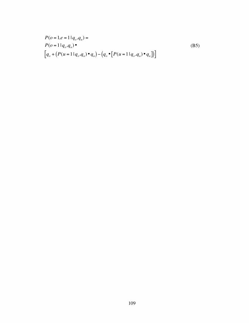
109

€

P(o =1,e =1 |qo,qu) =

P(o =1 |qo,qu)•

qo + P(u =1 |qo,qu)•qu( ) − qo • P(u =1 |qo,qu)•qu[ ]( )[ ](B5)

110

REFERENCES

Anderson, J. R. & Sheu, C. (1995). Causal inferences as perceptual judgments. Memoryand Cognition, 23, 510-524.

Baker, A.G., Mercier, P., Vallée-Tourangeau, F., Frank, R., & Pan, M. (1993). Selectiveassociations and causality judgments: The presence of a strong causal factor mayreduce judgments of a weaker one. Journal of Experimental Psychology:Learning, Memory, and Cognition, 19, 414-432.

Beckers, T., De Houwer, J., Pineno, O., & Miller, R. R. (2005). Outcome additivity andoutcome maximality influence cue competition in human causal learning. Journalof Experimental Psychology: Learning, Memory, & Cognition, 31, 238-249.

Beckers, T., Miller, R. R., De Houwer, J., & Urushihara, K. (in press). Reasoning rats:Forward blocking in Pavlovian animal conditioning is sensitive to constraints ofcausal inference. Journal of Experimental Psychology: General.

Bradley, P. S., Fayyad, F. M., & Reina, C. A. (1998, November). Scaling EM(Expectation-Maximization) clustering to large databases (MSR-TR-98-35).Redmond, WA: Microsoft.

Buehner, M. J., Cheng, P. W., & Clifford, D. (2003). From covariation to causation: Atest of the assumption of causal power. Journal of Experimental Psychology:Learning, Memory, & Cognition, 29, 1119-1140.

Bullock, M., Gelman, R., and Baillargeon, R. (1982). The development of causalreasoning. In W. J. Friedman (Ed.), The Developmental Psychology of Time (pp.209-254). New York: Academic Press.

Busemeyer, J. R. (1991). Intuitive statistical estimation. In N. H. Anderson (Ed.),Contributions to Information Integration Theory: Vol. 1. Hillsdale, NJ: Earlbaum.

Cheng, P. W. (1997). From covariation to causation: A causal power theory.Psychological Review, 104, 367-405.

Cheng, P. W., & Novick, L. R. (1990). A probabilistic contrast model of causalinduction. Journal of Personality & Social Psychology, 58, 545-567.

Cheng, P. W., & Novick, L. R. (1992). Covariation in natural causal induction.Psychological Review, 99, 365-382.

Cheng, P.W., Park, J., Yarlas, A.S., & Holyoak, K.J. (1996). A causal-power theory offocal sets. In D.R. Shanks, K.J. Holyoak, & D.L. Medin (Eds.), The psychology oflearning and motivation: Vol. 34. Causal learning (pp. 313-357). San Diego, CA:Academic Press.

Danks, D., Griffiths, T. L., & Tenenbaum, J. B. (2003). Dynamical causal learning. In S.Becker, S. Thrun & K. Obermayer (Eds.), Advances in Neural InformationProcessing Systems (pp. 67-74). Cambridge, MA: The MIT Press.

Dempster, A., Laird, N., and Rubin, D. (1977). Maximum likelihood from incompletedata via the EM algorithm. Journal of the Royal Statistical Society, Series B, 39,1–38.

Dennis, M. J., & Ahn, W. (2001). Primacy in causal strength judgments: The effect ofinitial evidence for generative versus inhibitory relationships. Memory andCognition, 29, 152-164.

111

Dickinson, A., Shanks, D., & Evenden, J. (1984). Judgment of act-outcome contingency:The role of selective attribution. Quarterly Journal of Experimental Psychology,36A, 29-50.

Goodie, A. S., Williams, C. C., Crooks, C. L. (2003). Controlling for causally relevantthird variables. Journal of General Psychology, 130, 415-30.

Griffiths, T. L., & Tenenbaum, J. B. (2005) Structure and strength in causal induction.Cognitive Psychology, 51, 354-384.

Waldmann, M. R., & Hagmayer, Y. (2001). Estimating causal strength: The role ofstructural knowledge and processing effort. Cognition, 82, 27-58.

Hagmayer, Y., & Waldmann, M. R. (2002). A constraint satisfaction model of causallearning and reasoning. In W.D. Gray, & C.D. Schunn (Eds.), Proceedings of theTwenty-Fourth Annual Conference of the Cognitive Science Society (pp. 405-410). Mahwah, NJ: Erlbaum.

Hagmayer, Y., & Waldmann, M. R. (2004). Seeing the unobservable - Inferring theprobability and impact of hidden causes. In K. D. Forbus, D. Gentner, T. Regier(Eds.) Proceedings of the Twenty-Sixth Annual Conference of the CognitiveScience Society (pp. 523-528). Mahwah, NJ: Erlbaum.

Holyoak, K. J., & Simon, D. (1999). Bidirectional reasoning in decision making byconstraint satisfaction. Journal of Experimental Psychology: General, 128, 3-31.

Hooke, R., & Jeeves, T. A. (1960). "Direct search" solution of numerical and statisticalproblems. Journal of the Association for Computing Machinery, 8, 212-229.

Jenkins, H. M., & Ward, W. C. (1965). Judgment of contingency between responses andoutcomes. Psychological Monographs: General and Applied, 79, 1-17.

Kelley, H. H. (1967). Attribution in social psychology. Nebraska Symposium onMotivation, 15, 192-238.

Lober, K., & Shanks, D. R. (2000). Is causal induction based on causal power? Critiqueof Cheng (1997). Psychological Review, 107, 195-212.

Lopez, F. J., Shanks, D. R., Almaraz, J., & Fernandez, P. (1998). Effects of trial order oncontingency judgments: A comparison of associative and probabilistic contrastaccounts. Journal of Experimental Psychology: Learning, Memory, andCognition, 24, 672-694.

Luhmann, C. C. & Ahn, W. (2003). Evaluating the causal role of unobserved variables.In R. Alterman & D. Kirsh (Eds.), Proceedings of the 25th Annual Conference ofthe Cognitive Science Society (734-739). Mahwah, New Jersey: LawrenceEarlbaum Associates, Inc.

Luhmann, C. C. (2005). Confounded: Causal inference and the requirement ofindependence. In B. G. Bara, L. Barsalou, & M. Bucciarelli (Eds.), Proceedingsof the 27th Annual Conference of the Cognitive Science Society (pp. 1355-1360).Mahwah, New Jersey: Lawrence Erlbaum Associates, Inc.

McClelland, J. L., & Rumelhart, D. E. (1981). An interactive activation model of contexteffects in letter perception: Part 1: An account of basic findings. PsychologicalReview, 88, 375-407.

McLachlan, G., & Krishnan, T. (1997). The EM Algorithm and Extensions. New York,NY: John Wiley and Sons.

McNemar, Q. (1947). Note on the sampling error of the difference between correlatedproportions or percentages. Psychometrika, 12, 153-157.

112

Morris, M.W. & Larrick, R, (1995). When one cause casts doubt on another: Anormative analysis of discounting in causal attribution, Psychological Review,102, 331-355.

Neal, R. M., & Hinton, G. E. (1998). A view of the EM algorithm that justifiesincremental, sparse, and other variants. In M. I. Jordan, (Ed.), Learning inGraphical Models (pp. 355-368) Cambridge, MA: MIT Press.

Novick, L. R. & Cheng, P. W. (2004). Assessing interactive causal influence.Psychological Review, 111, 455-485.

Pearl, J. (2000). Causality: Models, Reasoning, and Inference. New York, NY:Cambridge University Press.

Price, P. C., & Yates, J. F. (1993). Judgmental overshadowing: Further evidence of cueinteraction in contigency judgment. Memory and Cognition, 21, 561-572.

Read, S. J., & Marcus-Newhall, A. (1993). Explanatory coherence in social explanations:A parallel distributed processing account. Journal of Personality & SocialPsychology, 65, 429-447.

Rescorla, R. A., & Wagner, A. R. (1972). A theory of Pavlovian conditioning: Variationsin the effectiveness of reinforcement and nonreinforcement. In A. H. Black & W.Prokasy (Eds.), Classical Conditioning II. New York, NY: Appleton-Century-Crofts.

Schultz, L. E., Sommerville, J., & Gopnik, A. (2005). Casual determinism andpreschoolers' causal inferences. In B. G. Bara, L. Barsalou and M. Bucciarelli(Eds.), Proceedings of the 25th Annual Conference of the Cognitive ScienceSociety (1979-1984). Mahwah, New Jersey: Lawrence Earlbaum Associates, Inc.

Schustack, M. W., & Sternberg, R. J. (1981). Evaluation of evidence in causal inference.Journal of Experimental Psychology: General, 110, 101–120.

Shanks, D. R. (1989). Selectional processes in causality judgments. Memory andCognition, 17, 27-34.

Shanks, D. R., & Lopez, F. J. (1996). Causal order does not affect cue selection in humanassociative learning. Memory and Cognition, 24, 511-522.

Shanks, D. R. Holyoak, K. J., & Medin, D. L. (Eds.) (1996). The Psychology of Learningand Motivation (Vol. 34): Causal Learning. San Diego, CA: Academic Press.

Shanks, D. R., Lopez, F. J., Darby, R. J., & Dickinson, A. (1996). Distinguishingassociative and probabilistic contrast theories of human contingency judgment. InD. R. Shanks, K. J. Holyoak, & D. L. Medin (Eds.), In D.R. Shanks, K.J.Holyoak, & D.L. Medin (Eds.), The psychology of learning and motivation: Vol.34. Causal learning (pp. 265-311). San Diego, CA: Academic Press.

Schunn, C., & Wallach, D. (2002). In defense of goodness-of-fit in comparison of modelsto data. Unpublished manuscript, Pittsburgh, PA.

Simpson, E. H. (1951). The interpretation of interaction in contingency tables. Journal ofthe Royal Statistical Society, Series B, 13, 238-241.

Spellman, B. A. (1996). Acting as intuitive scientists: Contingency judgments are madewhile controlling for alternative potential causes. Psychological Science, 7, 337-342.

Steyvers, M., Tenenbaum, J. B., Wagenmakers, E., & Blum, B. (2003). Inferring causalnetworks from observations and interventions. Cognitive Science, 27, 453-489.

113

Suematsu, N., Maebashi, K., & Hayashi, A., (2004). An online variant of EM algorithmbased on the hierarchical mixture model learning. In M. H. Hamza (Ed.)Proceedings of the IASTED International Conference on Artificial Intelligenceand Applications, (pp. 270-275), Anaheim, CA: ACTA Press.

Tangen, J. M. & Allan, L. G. (2004). Cue-interaction and judgments of causality:Contributions of causal and associative processes, Memory and Cognition, 32,107-124.

Tanner, M. (1996). Tools for Statistical Inference (3rd ed.). New York: Springer Verlag.Thagard, P. (2000). Coherence in Thought and Action. Cambridge, Massachusetts: MIT

Press.Waldmann, M. R. (2000). Competition among causes but not effects in predictive and

diagnostic learning. Journal of Experimental Psychology: Learning, Memory, andCognition, 26, 53-76.

Waldmann, M. R. (2001). Predictive versus diagnostic causal learning: Evidence from anovershadowing paradigm. Psychonomic Bulletin & Review, 8, 600-608.

Waldmann, M. R. (1996). Knowledge-based causal induction. In D. R. Shanks, K. J.Holyoak, & D. L. Medin (Eds.), The Psychology of Learning and Motivation, Vol.34: Causal learning (pp. 47-88). San Diego: Academic Press.

Waldmann, M. R. & Hagmayer, Y. (2001). Estimating causal strength: The role ofstructural knowledge and processing effort. Cognition, 82, 27-58.

Waldmann, M. R., Holyoak, K. J., & Fratianne, A. (1995). Causal models and theacquisition of category structure. Journal of Experimental Psychology: General,124, 181-206.

Waldmann, M. R., & Holyoak, K. J. (1992). Predictive and diagnostic learning withincausal models: Asymmetries in cue competition. Journal of ExperimentalPsychology: General, 121, 222-236.

Wasserman, E. A., Kao, S. F., Van Hamme, L. J., Katagiri, M., & Young, M. E. (1996).Causation and association. In D. R. Shanks, D. L. Medin & K. J. Holyoak (Eds.),Psychology of Learning and Motivation, Vol. 34: Causal Learning (pp. 47-88).San Diego, CA: Academic Press.

White, P. A. (1992). Causal powers, causal questions, and the place of regularityinformation in causal attribution. British Journal of Psychology, 83, 161-188.

White, P. A. (2002). Causal attribution from covariation information: The evidentialevaluation model. European Journal of Social Psychology, 32, 667-684.

Widrow, B. & Hoff, M. E. (1960). Adaptive switching circuits, IRE WESCONConvention Record, 4, 96-104.

Documents

ii - ETD - Electronic Theses & Dissertationsetd.library.vanderbilt.edu/.../unrestricted/luhmann-dissertation.pdfno-confounding assumption (see Hagmeyer & Waldmann, 2004; Luhmann, 2005;