II D-Ai33 676 RESEARCH ON ADAPTIVE ANTENNA TECHNIQUES V,(U) STANFORD 1/2UNIV CA INFORMATION SYSTEMS LAB K M DUVALL ET AL.SEP 83 N00019-82-C-0i89

UNCLSIFIEDG 1714 N

liii&,8 JQ wW.,i * 2 J.2

mmli a * 00

125 m114 =

IEE'-

MICROCOPY RESOLUTION TEST CHARTNATIONAL BUREAU OF STANDARDS-1963-A

II

RESEARCH ON ADAPTIVE ANTENNA TECHNIQUES V

FINAL REPORT

by

Kenneth M. DuvallBernard Widrow

September 1983

Information Systems LaboratoryDepartment of Electrical Engineering D TC

Stanford University ELECTEStanford, CA 94305 ET

OCT 1760

D.This research was supported by the

Naval Air Systems Command of the Department of DefenseUnder Contract N00019-82-C-0189

APPROVED FOR PUBLIC RELEASE-, DISTRIBUTION UNLIMITED

. J The views and conclusions contained in this documentare those of the authors and should not be interpreted as

necessarily representing the official policies, either expressed or impliedof the Naval Air Systems Command or the U. S. Government.

W. "- V V -. " '. . .

, (F R

-ii -

ABSTRACT

- I

Adaptive antennas provide an important means of enhancing signal-to-noise

ratio in the adverse electromagnetic environments that sometimes arise due to

jamming or interference. For that reason, adaptive antennas are increasingly

finding application in high performance radar and communications systems. In

many of these systems the adaptive subsystem must exhibit robust performance

in the face of multipath or rapidly changing interference.

Unfortunately, the adaptive beamformers now in use do not perform well in

certain environments. It has been known for some time that correlated-signal

conditions (e.g., due to multipath) can lead to partial or total cancellation of the

desired signal within :'n adaptive beamformer. More recently it has been

recognized that signal cancellation can arise, during high-speed adaptation even

though 1) the desired signal and interfering signals are uncorrelated and 2) the

look-direction response is rigidly controlled. The initial sections of this report

examine the signal-cancellation mechanism, with emphasis on the more difficult

uncorrelated-signal case. Simulation results are presented that illustrate the

cancellation effect, and an analysis is given for a simple environment consisting of

the desired signal and one jammer.

The remaining sections of the report describe a technique for avoiding signal

cancellation. The adaptation problem is reformulated to permit jammer nulling

and signal recovery under conditions that ordinarily result in signal cancellation.

APPROVED FOR PUBLIC RELEASFsDISTRIBIJIh UO LM=

'j. iii -

The reformulated problem suggests a new adaptive structure comprised of a

*master beamformer in which adaptation is conducted in a synthetic, signal-free

environment and a slaved beamformer in which the actual array-element signals

are processed. The new structure, which is termed a composite beamformer, is

compared to Frost's hard-constrained adaptive beamformer. Particular attention

is given to relative performance in cancellation environments, to conditions under

which optimal behavior is approached, to convergence speed, and to weight

behavior near convergence.

Accession For

DTIC TAB 0Unarounced 0Justif ioatio_ ,

Distribut..o._

AvailabilItY Codes

Avail d/o "rDIat Speolal

7:FtI9:

* G~~OO ~)

-I-.

TABLE OF CONTENTS

Page

I. INTRODUCTIO N .............................................................................. I

H. SIGNAL CANCELLATION INHARD-CONSTRAINED BEAMFORMERS ................................ 4

A . Background ...................................................................................... 5B. Frost's Constrained LMS Algorithm ................................................ 7C. Signal Cancellation in the Wideband Case ...................................... 14D. Signal Cancellation in the Narrowband Case ................................... 21E. An Equivalent Adaptive-Noise-Cancelling Problem ........................ 32

I. A COMPOSITE BEAMFORMER THAT ELIMATESSIGNAL CANCELLATION ............................................................ 42

A. Problem Reformulation .................................................................... 42B. Signal Relationships in the CBF

M aster and Slave ............................................................................. 47C. CBF Performance - An Example .................................................... 54

IV. PERFORMANCE OF THE COMPOSITE BEAMFORMER 60

A. CBF Optimality in the Narrowband Case ....................................... 60B. Further Simulation Experiments with the CBF .............................. 68C. Convergence Time Constants .......................................................... 72D. W eight Quieting in the CBF ............................................................ 78

V. SUMMARY AND CONCLUSIONS ............................................. 83

REFERENCES .......................................... 86

APPENDICES ............................................ go

A. Analysis of the Dynamic Solution forthe Sinusoidal Case .......................................................................... 90

B. An Alternative Expression for theOptimal W eights in a Frost ABF .................................................... 101

C. An Analysis of Signal Influence Based Uponthe Generalized Sidelobe Canceller .................................................. 110

D. A Composite Beamformer Based UponW idrow's Plot-Signal Algorithm ...................................................... 114

E. Sim ulation M ethods ......................................................................... 129

q '" ,' ' : ::, . " '-'- "'/ "" i- -: " _i i i" ' ' •" " :: " " : ' ,

5', ,- . ' - - -. . . . • , . .' o , . -, - . . . . . . - - . - . ,. , .'. . , . .- -

IV

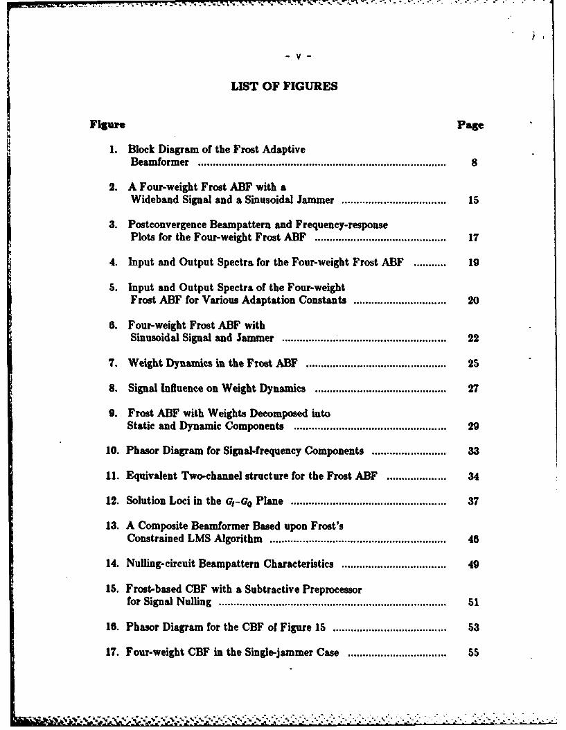
LIST OF FIGURESFigure Page

1. Block Diagram of the Frost AdaptiveBeamformer ........................................... 8

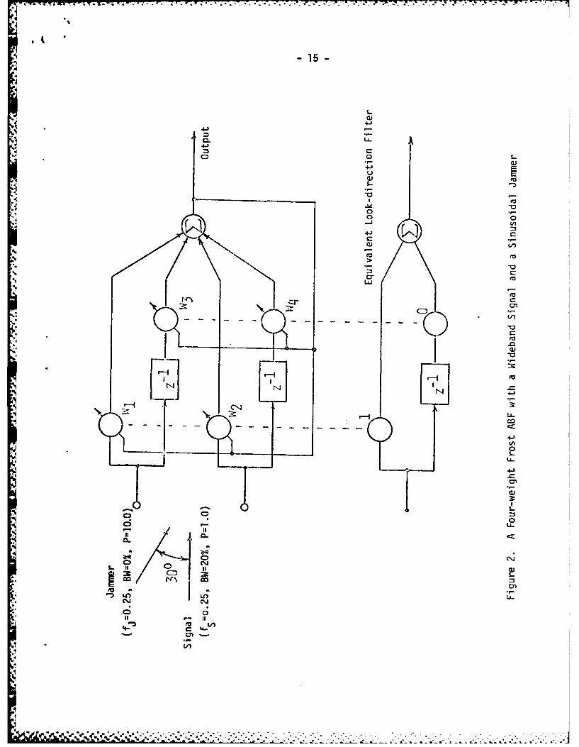
2. A Four-weight Frost ABF with aWideband Signal and a Sinusoidal Jammer ................................... 15

3. Postconvergence Beampattern and Frequency-response

Plots for the Four-weight Frost ABF ............................................ 17

4. Input and Output Spectra for the Four-weight Frost ABF ........... 19

5. Input and Output Spectra of the Four-weightFrost ABF for Various Adaptation Constants ............................... 20

5. Four-weight Frost ABF with

Sinusoidal Signal and Jammer ............................ 22

7. Weight Dynamics in the Frost ABF ............................................... 25

8. Signal Influence on Weight Dynamics ............................................ 27

9. Frost ABF with Weights Decomposed intoStatic and Dynamic Components ................................................... 29

10. Phasor Diagram for Signal-frequency Components ......................... 33

11. Equivalent Two-channel structure for the Frost ABF .................... 34

12. Solution Loci in the G,-GQ Plane .................................................... 37

13. A Composite Beamformer Based upon Frost'sConstrained LMS Algorithm ........................................................... 46

14. Nulling-circuit Beampattern Characteristics ................................... 49

15. Frost-based CBF with a Subtractive Preprocessor

for Signal N ulling ............................................................................ 51

16. Phasor Diagram for the CBF of Figure 15 ...................................... 53

17. Four-weight CBF in the Single-jammer Case ................................. 55

-vi-

18. Postconvergence Beampattern for the Four-weightCBF in the Single-jammer Case ................................................... 56

19. Input and Output Spectra for the Frost ABF and theFrost-based CBF .......................................................................... 58

20. Comparison of ABF and CBF Output Signals ............................ 59

21. Four-weight CBF in the Two-jammer Case ................................. 70

22. Postconvergence Beampattern for theFour-weight CBF ........................................................................ 71

23. Six-weight CBF in the Two-jammer Case .................................... 73

24. Postconvergence Beampattern Plot for theSix-weight CBF ............................................................................ 74

25. Comparison of ABF and CBF Convergence Timesin the Single-jammer Case ........................................................... 77

26. ABF and CBF Error Curves Near the Optimal Weight .............. 82

A-i. Equivalent Adaptive-Noise-Canceller

Representation ............................................................................... 91

A-2. Plot of Sinc Function Magnitude and an Upper Bound ............... 97

C-1. Block Diagram of a Griffiths-Jim Sidelobe Canceller .................... III

D-1. Diagram of an M-stage Nulling Tree ............................................ 117

D-2. Nulling-tree Beampattern Plot with Nullsat -0 , 0 , and 45 ........................................................................ 118

D-3. Nulling-tree Beampattern Plot with BroadenedN ull at 0 ....................................................................................... 120

D-4. Block Diagram of the Pilot-signal CBF ........................................ 121

E-1. Flowchart for Adaptive Antenna Simulation ................................ 131

E-2. Flowchart for Generation and Plotting ofAntenna Responses ........................................................................ 135

E-3. Flowchart for Generation and Plotting ofInput/Output Signals ............... .................................................... 138

-,. . . . ".' ' - " . . , - .

- - - -* ~

L INTRODUCTION

The past two decades have witnessed the emergence of the adaptive antenna

as an important element in countermeasures-resistant radar and communications

systems. The application that has inspired most of the development effort is

jammer nulling; adaptive antennas can eliminate a substantial fraction of the

incident jammer power while admitting some desired signal (or signals) with

useful gain. A key aspect of this selective treatment of jammers and desired

signals is that it is accomplished without extensive a priori knowledge of the

jammer environment. Instead, the locations of jammers are "learned" by some

adaptive algorithm, and nulls are automatically steered to and maintained on the

jammers.

One of the fundamental issues in adaptive antennas has been signal

preservation. It has been clear from the beginning that the nulling behavior

which is of such great value in eliminating jammers is a two-edged sword that

also threatens the desired signal. Proper control is absolutely essential to avoid

signal loss in the adaptive beamformer (ABF). The original sidelobe-canceller

scheme of Howells and Applebaum 11,2] exploited the differing signal-to-jammer

ratios in a directive primary antenna and an omnidirectional auxiliary antenna to

avoid seriously attenuating desired radar signals. Widrow [31, operating with

somewhat different signal and antenna assumptions, took the tack of introducing

pilot signals to control beamformer response in specified look directions. Griffiths

[4] devised a different soft-constraint technique that involved statistical

r7;

-2-

characterization of the desired signals rather than the actual surrogate signals

required by the pilot-signal scheme. Frost 15,61 developed a constrained least-

mean-square (LMS) algorithm that assured exact conformance with some

prespecified look-direction response. More recently, Griffiths and Jim 17,8]

contributed a structure called the "generalized sidelobe canceller," which

provided an alternative method of realizing hard constraints. Some further

development and generalization of soft-constraint methods has also taken place

within the past few years; Chestek [9) brought together much of the earlier work

on soft-constrained methods by combining soft linear constraints with a mean-

square-error criterion in his soft-constrained LMS algorithm.

A unifying factor in the work just outlined is the focus on the response of

the antenna to desired signals. This approach involves a tacit assumption that

the problem decomposes in a tractable way, i.e., that desired signals and jammers

can be treated independently. The assumption can be justified in many cases,

but, as will be demonstrated, there are some rather simple signal/jammer

scenarios where difficulty arises. When a failure occurs, the usual constraint

methods do not adequately protect the desired signal. Instead, the signal is

partially or totally destroyed in the adaptive beamformer by residual jammer

signals. This phenomenon is termed signal cancellation.

'* The remainder of this report is devoted to a further discussion of signal

cancellation and to the description of a method for avoiding it. The next chapter

N :

-3-

provides insight into the signal cancellation phenomenon by explaining how it

was recognized and by showing the effect in two simple cases. Chapter MI

introduces a composite beamformer that defeats signal cancellation and

demonstrates the performance improvement that it provides. Chapter IV

elaborates upon the characteristics of the composite beamformer by describing

convergence behavior, illustrating performance under additional signal conditions,

and examining the issues of convergence rate and weight behavior near

convergence. Finally, Chapter V summarizes the status of the work on signal

cancellation and lists some topics that deserve further research.

-4-

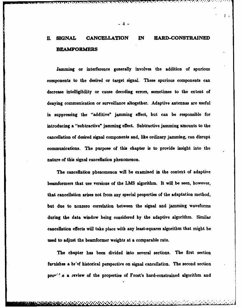
I. SIGNAL CANCELLATION IN HARD-CONSTRAINED

BEAMFORMERS

Jamming or interference generally involves the addition of spurious

components to the desired or target signal. These spurious components can

decrease intelligibility or cause decoding errors, sometimes to the extent of

denying communication or surveillance altogether. Adaptive antennas are useful

in suppressing the "additive" jamming effect, but can be responsible for

introducing a "subtractive" jamming effect. Subtractive jamming amounts to the

cancellation of desired signal components and, like ordinary jamming, can disrupt

communications. The purpose of this chapter is to provide insight into the

nature of this signal cancellation phenomenon.

The cancellation phenomenon will be examined in the context of adaptive

beamformers that use versions of the LMS algorithm. It will be seen, however,

that cancellation arises not from any special properties of the adaptation method,

but due to nonzero correlation between the signal and jamming waveforms

during the data window being considered by the adaptive algorithm. Similar

cancellation effects will take place with any least-squares algorithm that might be

used to adjust the beamformer weights at a comparable rate.

The chapter has been divided into several sections. The first section

furnishes a br'of historical perspective on signal cancellation. The second section

prop' "s a ieview of the properties of Frost's hard-constrained algorithm and

-5-

establishes notation that will be useful throughout the report. The third section

discusses the effects of signal cancellation on a wideband signal and illustrates the

destruction of signal components that can occur. The final two sections consider

cancellation in the narrowband case. Appendix A contains a supporting analysis

2 for the final section.

A. Background

It has been realized for some time that signal cancellation can occur even in

hard-constrained beamformers when correlation exists between the desired signal

and some other signal impinging upon the array. (See, for example, [61 by Frost.)

This was a disquieting fact, because this is precisely the condition that can arise

naturally as a result of multipath or can be induced artificially through repeater

jamming. It appears, however, that this troublesome case was more or less set

aside" while work continued on other aspects of adaptive antennas.

As adaptive-antenna work went forward in other areas during the mid-

seventies, developments relevant to signal cancellation were taking place in

another branch of adaptive systems. Experimental work in adaptive noise

cancellation had disclosed filtering phenomena that fell outside the purview of

Wiener filter theory. Glover [10,11,121 analyzed this non-Wiener behavior and

0 ome work directed specifically toward adaptive elimination of multipath interference at HF was described inNovember 1981 by Hasten and Loughlin 101. Their method makes use of a modulated pilot signal that is added to thecommunication signal at the transmitter. Pilot bandwidth must be adequate to provide discrimination between the vari-one modes arriving at the receiver. This approach is limited to those situations where the transmitter is accessible andbandwidth allocations are not restrictive.

showed that, for the case involving sinusoidal reference inputs, the adaptive noise

sccesflle a be regarded as a stable notch filter. Shensa 113,141 was later

sucessulin treating a somewhat more general class of input signals.

Widrow was able to extrapolate from the work being done on adaptive noise

cancellers and draw some disturbing new conclusions concerning signal

cancellation in adaptive beamforiners. Widrow realized that correlation (in the

usual long-term sense) was a sufficient, but not neceseary, condition for the

destructive effects of signal cancellation. If high adaptation speeds are employed,

signal cancellation can be induced by a broad class of jammer signals, and close

replication of the desired signal (e.g., through repeater jamming) is not

necessarily required. Since high adaptation rates are being sought so that good

jammer nulling performkance can be obtained in dynamic countermeasures

environments, the conditions that support signal cancellation may be routinely

present. Recognition of this state of affairs added considerable incentive to study

signal cancellation. Simulation work was begun at Stanford in 1980 to confirm

the effects predicted by Widrow and to support the search for methods of

avoiding signal cancellation. Portions of this work have been reported in

-~ References 15 and 18. Other workers [17,181 have observed signal cancellation in

actual adaptive-antenna systems.

-7-

B. Frost's Co=trained LMS Algorithm

The application of his constrained LMS algorithm to adaptive arrays has

been described in some detail by Frost [5,6J. Some of the key results will be

restated in this section to provide the background and notation for discussions

that follow.

The adaptive array problem to be considered is pictured in Figure 1. A

uniform linear array of K elements is connected to an adaptive beamformer

that consists of K tapped-delay-line filters, each with J taps and J

adjustable weights. The sampled tap voltages and the weights are indexed in the

columnar scheme shown in the figure and are identified in vector notation as~Xr'M Ar 1-- ), -T2(A, .. -KAA~ (2-1)

WTj) . [w1(j), w 2(j), ... , wK1(j)] , (2-2)

where j is the sample number. The filter outputs are summed to form the

beamformer output:

y(j) = WT(j)X(j) - XT(j)W(j) (2-3)

. In addition to being the useful output signal from the system, the

beamformer output serves as the error signal that is fed back for use in the

weight adaptation process. The goal of adaptation is to minimize the output

contribution of noise sources (such as the jammer indicated in the figure), subject

*4t

.9 e" ' f ,L .. ./ ,2 ._ "".J _," :, ," "' ' "" " ' ' "" " "

7-8

44n

44J

a)caci

L. m

S- LL

0

C1 t9-. -<

LUm

t) (0 <T

so---

ago.

coL

CU

I/~-

-9-

to a set of constraints that provide rigid control over the array response in the

direction from which desired signals are expected.

It is assumed that the desired signal and the interference are uncorrelated.

The incident signal vector may be decomposed according to

X(j) = S(j) + N(j) (2-4)

by letting S(j) represent the vector of desired signals at the beamformer taps

and N(j) represent the aggregate contribution of the various noise sources. If

the autocorrelations of the quantities of Eq. 2-4 are defined by

RXX . E[X(j) XT(j)] (2-5)

Rss A. E[S(j) ST(j)] (2-6)

RNN . E[N(j) NT(j)I , (2-7)

then the assumed lack of correlation between the desired signal and the noise is

expressed by

RXX = RSS + RNN (2-8)

This correlation condition must hold if the look-direction constraints are to afford

protection for the desired signal.

The constraint method depends upon knowing the arrival direction of the

desired signal. The array is assumed to be steered (either mechanically or

m . *- f r.• ° • - . • , . % -. . , • . .- .°. . . . , • . • ....- . - . °. . ° - o° -

- 10-

electrically) toward the known look direction. Under this assumption, the desired

signal components are identical at the inputs to the beamformer filters and along

any column of taps in the beamformer. An equivalent look-direction processor

can therefore be formed by summing the weights in each beamformer column to

arrive at the J-tap filter shown at the top of Figure 1. The equivalent look-

direction filter provides the key to an algorithm that minimizes noise

contributions at the output without influencing the response to the desired signal.

Specifically, the weights may be freely adjusted to minimize the noise output

provided the column sums in the beamformer remain equal to the preselected

weights in the equivalent look-direction processor. In order to state the

minimization problem succinctly, it is helpful to express the look-direction

impulse response in vector form and to define a constraint matrix. The look-

direction-response vector is formed from the weights in the equivalent look-

direction filter:

I AII1, 12, f.., 1J (2-0)

o.5.

y.

..

5,. . . . . . . . . . . . . . . *

* - 11 -

b75

The constraint matrix C is composed of columns of the form

0

0

0 } (i-1)"group of K elements

0

1 igroup of K elements

cl= 11

0

O (i+ 1)" group of K elements

0

0* : jigroup of K elements

0(2-10)

That is,

]C

C...[c , c , ... , *. ], (2-11)

The matrix C is a KJ X J matrix that conveys the beamformer structural

information needed to implement the constraints.

With the notation developed to this point, the constrained-LMS problem

may be stated:

- 12-

Minimize Efy(j)] = EIWTX(j)XT(j)W = WTRXXW (2.12)W

subject to CTW -

Frost developed both closed-form and adaptive solutions for the

constrained-LMS problem. The method of Lagrange multipliers was used to

arrive at the optimal solution in terms of the signal statistics and the constraints:

WO = RAJC[C "TRJC ]- L (2-13)

This solution assumes that the signal statistics are known (or have been

estimated) and imposes a heavy computational burden if the matrix inversions

must be repeatedly performed to track a dynamic environment.

The adaptive algorithm generates an asymptotically optimal solution to the

constrained-LMS problem and requires much less computation per weight-update

cycle than the closed-form solution. The update scheme is most easily

understood from the individual weight recursions:

IKw1(j+ 1) = w,(J) - Py(J)z,(f) - -,(j) + '

K im

-L K Aiffi -[wj) -pyJ) -(i) d)

w K+ (j+ 1) =w K+ I) -Pyj)Z-K+ ,j) [W - P(( + K2s-Kg- K

:.7

II h

WKJ(j+ 1) = w.4jU) - PYU)--xnr(J- i [w(j) +

K K,[ij Y

.1'*

":' ~wKJlJ+ 1) -- wKJ(J) - ps(J4rK,(J) K " . [w(j) - o~'J~'~j' + K-

(J-I)K+ 1

(2-14)

The right-hand side of each recursion involves the current weight value plus

several update terms. The first update term depends upon the current error and

the signal at the weight in question. The adaptation constant p is used to scale

this term; p is set* to yield stable system operation and to provide an

appropriate adaptation rate. The second update term is the average correction

over a column of weights, and the third update term is a fractional allocation of

the appropriate weight in the equivalent look-directional filter. Taken together,

the three update terms drive the weights toward the values that minimize output

power subject to the specified linear constraints. It is easy to verify the efficacy

of the constraint method by summing the updated weights over any column of

the beamformer and noting that the constraint is always satisfied.

The constrained-LMS algorithm may be written in matrix form to provide a

more compact description. It is helpful to introduce a KJ-dimensional initial

weight vector F, where

Futor governing the choice of i are discussed in References 6, S, and to.

*'. oo . , ' "° . a° .'° - . " " - ° . ° f ° - . -. .. . a . .. • - -. . . ' - o . . . .. . -

** " •* ' " " ".. . . ." " ". a"- '." . .". -" "'.

-14-

F A C(CTC)-1 (2-15)

and a KJ X KJ projection operator P, where

P =& I - C(CTC)-ICT , (2-1)

With this added notation, the constrained-LMS algorithm may be stated as:

W(O) = F

W(j+ 1) = P[W(j)-py(j)X(j)] + F (2-17)

It will also be useful to note the time constants exhibited by the hard-

constrained algorithm. Frost showed that the matrix P RyxxP determines the

rate of convergence of the mean weight vector toward the optimal weight vector

W. Specifically, convergence of the mean weight vector along the ii"

eigenvector of P RXXP occurs with a time constant given by

Ti 1 1 1in( l-pai) - p(i

where oru is the eigenvalue associated with the ilk eigenvector and where

updating at the sample rate (as opposed to, say, every tenth sample) is assumed.

C. Signal Cancellation In the Wideband Case

, The effects of signal cancellation in a hard-constrained ABF can be readily

demonstrated by simulating* the simple adaptive-antenna problem diagrammed

in Figure 2. The selected adaptive antenna was a two-element Frost ABF with

0As overview of the simulation methods used in this research is given in Appendix E.

.44

4-

17

44

L

U--

.44J

0 0

4.4)

Uc

00

co 0e

too

CMC

-16-

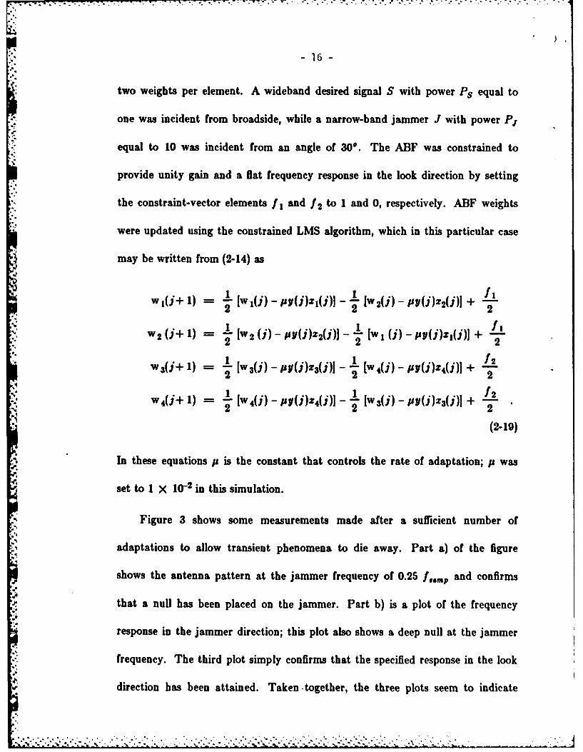
two weights per element. A wideband desired signal S with power Ps equal to

one was incident from broadside, while a narrow-band jammer J with power Pr

equal to 10 was incident from an angle of 30'. The ABF was constrained to

provide unity gain and a flat frequency response in the look direction by setting

the constraint-vector elements f and 12 to 1 and 0, respectively. ABF weights

were updated using the constrained LMS algorithm, which in this particular case

may be written from (2-14) as

w (J+ 1) 1 1 - (J l - . [w 2 Uj) - P Y()z 2(i)] + LI2 [w1(j) - 2 2

222w(j+ 1) = 17 [w (j) -PYi) 2(i)]- - () -PYU)Z4U)I + 2

w 3 (j+ 1) = - [ 31 ) - pYUj) 3(j)J - - [w U) - Pyli)z4 (i) + L2

2 2 2I.= ~ [w 41( sll4() "[j) - - 12(~3() I

w'i 11 w= iI-

(2-19)

In these equations p is the constant that controls the rate of adaptation; p was

set to I X 10-2 in this simulation.

Figure 3 shows some measurements made after a sufficient number of%',

-, adaptations to allow transient phenomena to die away. Part a) of the figure

shows the antenna pattern at the jammer frequency of 0.25 l,,,, and confirms

that a null has been placed on the jammer. Part b) is a plot of the frequency

response in the jammer direction; this plot also shows a deep null at the jammer

frequency. The third plot simply confirms that the specified response in the look

direction has been attained. Taken -together, the three plots seem to indicate

T--:- ~ ~ ~ ~ -0797 17.-,77

-.17- Signal

Jammer

OdB/

-40dB

a)

-40.0

0.0 0.1 0.2 0.3 0'4 0!5

b) Frequency

.-. 0.0

C

-40.0

0.0 0.1 0.2 0.3 0.4 0.5

c) Frequency

Figure 3. Postconvergence Plots for the Four-element Frost AGFa) Beampatternb) Jammer-direction Frequency Responsec) Signal-direction Frequency Response

v. . . . . . ... . . . . .. . . . . . . - ... - -

-~_w -111 7P 7~. 'Y .i. q..O -... ~ ~ 7 7 - -* -~ - - -W

-18-. 3

that all is well and that the intended objectives of signal recovery and jammer

rejection have been attained.

The favorable picture provided by the antenna plots of Figure 3 darkens

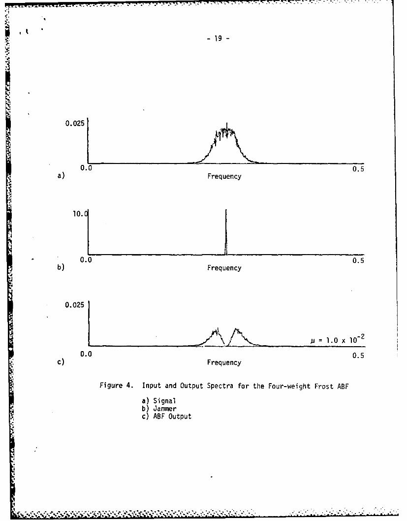
considerably when the desired signal and the ABF output are compared. Figure

4 is a plot of ensemble- averaged spectra of the desired signal, the jammer signal,

and the ABF output. It is clear that, despite very rigid control of the look-

direction response and good jammer rejection, the desired signal has not been

recovered intact. Instead the signal has experienced frequency-dependent

distortion. Signal components on the skirts of the signal remain unaffected, but

components in the vicinity of the jammer frequency have been totally or partially

destroyed in the ABF.

I The extent of signal cancellation for a given antenna structure and signal

environment is governed by the rate of adaptation, i.e., by the adaptation

parameter p. The simulation just described was repeated for several different

values of p; output spectra for the series of experiments are assembled in Figure

S. Parts a and b of the figure involve lower adaptation rates than the rate used

to produce the results in Figure 4 and reveal lesser amounts of signal destruction.

In fact, cancellation is almost undetectable in Part a. Part c repeats the results

shown in Figure 4. Part d involves a large pa (a value near the instability point)

and shows the near-total signal destruction that can occur in an extreme case. It

is apparent from Figure 5 that cancellation occurs over a considerable range of

adaptation parameter selections and that the destructive effects can be quite

-19-

0.025

0.0 0.5

a) Frequency

"10.1

- 0.0 0.5b) Frequency

0.025

0.0 0.5

c) Frequency

Figure 4. Input and Output Spectra for the Four-weight Frost ABF

a) Signalb) Jammerc) ABF Output

M ° '

77 %W'V-2-20-

.025

*&, =1.0 x 10-4

a) 0.0 Frequency 0.5

.025

0.05 = 1.0 x 10-3

b) 00Frequency 0.5

* .025

I p =1.0 x 1O-2

0.0 0.5Frequency

.025

$' p =8.0 x 10-2

0.0 0.5

d) Frequency

Figure 5. Output Power Spectra of the Four-weight Frost ABF

for Various Adaptation Constants

-21-

important when high adaptation rates are sought. It is also clear that, although

cancellation effects may be made negligible by choosing a sufficiently small p,

orders of magnitude in convergence rate must be sacrificed to maintain signal

quality. At these low adaptation rates the ability to track a dynamic

environment will be greatly reduced.

D. Signal Cancellation in the Narrowband Case

A wideband signal was useful in the examples of the previous section

because the broad spectrum clearly showed the extent of cancellation effects.

This section will concentrate on developing a more detailed picture of the

cancellation phenomenon by considering the internal operation of a beamformer

* while cancellation is occurring. A narrowband signal as well ' a narrowband

jammer will be used to facilitate the analysis of beamformer behavior.

A particularly simple beamformer structure and signal/jammer scenario were

sought to provide a test case for the study of cancellation effects in the Frost

ABF. The selected problem is illustrated in Figure 6, which shows a sinusoidal

desired signal S (frequency fs = 0.25) incident on a two-element array from

broadside and a sinusoidal jammer J (frequency f- = 0.26) incident from 45*.

Element spacing was a half wavelength at the signal frequency. The antenna

elements were tied to a four-weight Frost ABF that was steered to broadside and

constrained to provide unit gain and flat frequency response in the look direction.

(The constraints were f 1 1 and /2 = 0, as indicated in the equivalent look-

.1 %- • " 'Y ' ; m -m -

-22-

4~) 4

C)C

0

4-)

CL

-Ha

zrr

0- -v

C-C

C)

'-1-

4.)

0S..

.a

0)

00

If',

cl-i

V) c)

-1 7 74. . . . . . .'i., , ,=._ l. -o, ,. . . ,- % .. ", .. -, -' ." - . b,- -° * - .o

- - "- - -' -

-23-

direction filter.) The weights were updated using the constrained LMS algorithm

given in Equations (2-19).

Just enough degrees of freedom were provided in this test case to allow the

objectives of signal reception and jammer rejection to be realized. Constant gain

in the signal direction was assured by the hard constraints of the Frost

algorithm:

W 1 + W 2 = 1I w +w =O(2-20),-W 3 + W 4 = 0 (-0

The constraints consumed two of the four available degrees of freedom; the

remaining two degrees of freedom were adequate for eliminating the jammer.

The requirements for eliminating jammer energy can be readily derived for

the simple case at hand. The array output attributable to the jammer is given

by

YA(t= ewi [WI-jw3] + ei(w" )[w 2 -jwj (2-21)

where 4'e is the element-to-element phase shift for the jammer signal. The

element-to-element phase shift may be computed from the array geometry and

the signal and jammer parameters:

21r J sin 45 21r sin 45*

.'ee = - ---- 2.31 radians (2-22)

_(25

Inserting the value for ,, expanding, and equating real and imaginary parts to

-24 -

zero yields

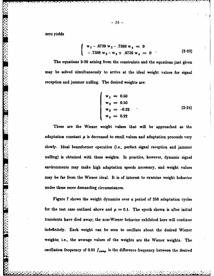
W1 w- 673g W2 -. 7388 W4 =0

- .7388W2 - W3 + .6739gW 4 = 0 2-3

The equations 2-20 arising from the constraints and the equations just given

may be solved simultaneously to arrive at the ideal weight values for signal

reception and jammer nulling. The desired weights are:

w 0.50

W2 = 0.50

W3= -0.22 (2-24)

W4= 0.22

* These are the Wiener weight values that will be approached as the

adaptation constant p is decreased to small values and adaptation proceeds very

slowly. Ideal beamformer operation (i.e., perfect signal reception and jammer

nulling) is obtained with these weights. In practice, however, dynamic signal

environments may make high adaptation speeds necessary, and weight values

may be far from the Wiener ideal. It is of interest to examine weight behavior

under these more demanding circumstances.

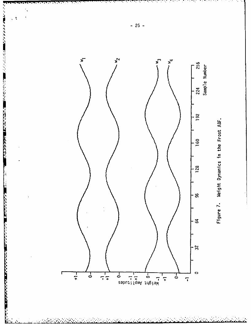
Figure 7 shows the weight dynamics over a period of 256 adaptation cycles

for the test case outlined above and p =0.1. The epoch shown is after initial

transients have died away; the non-Wiener behavior exhibited here will continue

indefinitely. Each weight can be seen to oscillate about the desired Wiener

weights; i.e., the average values of the weights are the Wiener weights. The

oscillation frequency of 0.01 is the difference frequency between the desired

-25-

*1cn

IL

c.C14 E~.

3 3 3ChU, co

000

o L

9- 0)

cl-cCY))

+ + Isapnj dwV q~ta

-26-

r- signal at 0.25 f...p and the jammer signal at 0.26 l.,rn.p This is the same

weight behavior noted by Glover [11,121 in a related noise-cancelling problem.

Figure 8 documents the behavior of the weights when the simulation

experiment is altered by abruptly switching off the signal at the time indicated.

The oscillatory behavior of the weights ceases, and, after a brief transient period,

the weights reach and hold the optimal values that were calculated earlier. It

thus appears that signal energy is needed to support the non-Wiener behavior

that has been observed. The precise role of the signal in the adaptive system

may be better understood by examining the interactions of the desired and

jammer signals and the dynamic weights.

From Figure 7 it is clear that during signal presence each of the weights is of

the form

W i = Ci + Ai sin(wAt + i) , (2-25)

where C is a constant giving the mean weight value, w, = (27r)(0.01 ferP) is

the radian difference frequency, and Ai and Oi are constants expressing the

amplitude and phase of the sinusoidal component of the weight. Arbitrarily

selecting w I as the phase reference and measuring the remaining constants yields

the following expressions for the weights:

4

* AI '**t '. . .- * . *. . . . . . . . o. . .. ... .. ..

-27-

'II

cNJ

CYI

0 IA~

4- u

Io S-

'i o)-0

E 4-)

.4L

CDi C C)+~ .I +0

sapnjLdwV 46LE

28-

w 0.50 + 0.46 sin (wt-4,)W 2 = 0.50 + 0.40 sin (w4 t-4o-r)W3 = -0.22 + 0.46 sin (wt-O-r/2) (2-26)

W 4 = 0.22 + 0.46 sin (wt-,4-32'/2)

Note that the oscillations of weights w I and w 2 are 180* out of phase so that the

hard constraint for these two weights is always satisfied. Similarly, weights w 3

and w 4 are antiphased and satisfy the constraint at all times.

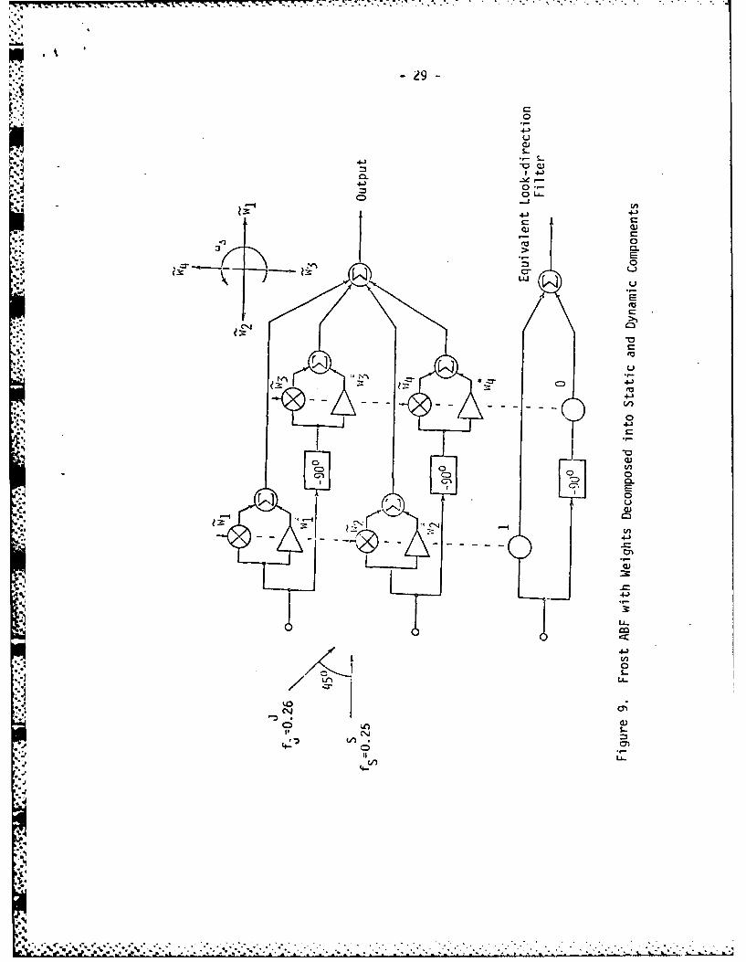
For purposes of analysis the beamformer of Figure 6 may be redrawn to

reflect the observed nature of the weight behavior. Figure 9 shows a revised

structure in which each weight has been replaced by the parallel combination of a

fixed gain and a mixer. The fixed gains are set to the Wiener weights as required

by the observed average values of the weights. The mixers have introduced into

them a set of sinusoidal voltages with radian frequency equal to W&, as required

by the observations regarding the oscillatory component of the weights. The

relative phases of the mixer input voltages are shown in the phasor diagram inset

into the upper right of the figure.

It is evident from Figure 9 that the oscillatory behavior of the weights

creates a considerably more complicated signal set in the adaptive beamformer

than would be the case with constant weights. The fixed gain associated with

each weight contributes one component at the signal frequency and a second

component at the jammer frequency. The mixer, however, yields sum and

difference components for both the signal and the jammer. The net contribution

Z;! .;. .? °. ?????. ? o. -- ?i--?-- --- -: .- ; • -

-29-

41.

4J4

44-3

e= 0*o Li.

:3 C

CE

LM

4)

4)

Ii 0

CDCI I.

-30-

from each weight is six components at four different frequencies; the signal set

* entering the final summing junction in Figure 9 consists of 24 different

components. A detailed examination of these components is necessary to

understand signal cancellation in even this simple case.

Fortunately, the apparent complexity of the 24-signal set is greater than its

actual complexity. First, it should be recalled that the Wiener weights are

known in this case to provide perfect signal reception and perfect jammer nulling.

It follows that the eight components attributable to the fixed gains combine to

simply yield a single component equal to the desired signal as seen at either array

element. Second, it should be noted that in both beamformer columns (i.e. at

weights w I and W 2 and at weights W 3 and W 4) the desired signal is cophased

while the weights are antiphased. All eight terms arising from mixer action on

the desired signal therefore sum to zero in the output summing junction. It

should be noted that components generated from the desired signal by weight

dynamics will always cancel in a properly steered Frost ABF due to the phase

* relationships enforced by array steering and the hard constraints.

At this point the only components that have not been examined are those

generated by mixer action on the jammer signals. The output signal may be

written as

-31

S=t) cos Wst

+ Icos w1 t]lA sin(wAt - 'o)]

+ [cos(wt - 0,) [A sin(wAt - 0o - r)l

+ [sin wjrtj [A sin(wAt - 00- 7r/2)]

+ [sin(w t - 0,)] [A sin(,At - 0o - 3ir/2)] (2-27)

where A is the amplitude of the weight oscillations. Expanding the products of

signals and weights yields

.4

.4 Y(t) = cos WS t

A Asi[_s t _ o

+ -1 sin[(w,& + w )t - 0o1 + A sin[(-ws)L - 0012 2

+ -" sin[(w& + w4t - - -1 + A sin[(-ws)t - 0o + 0,, - irl2 2

AAsi(.s t _ o2'A sin[(w + w1)t - 40] + A sin[(-WS)t -001

A sin[(w, + w )t - 0 4-Oe - 7] + A sin[(-ws)t - 0o + -

2 2(2-28)

Further simplifications are obvious at this point. Cancellation eliminates all

the terms at the radian frequency (w,& + w1 ). Additionally, terms at -"'s can be

combined and then reexpressed using the relationship

sin(-0) = - sin(0) . (2-29)

These steps plus inserting the measured value of A yield

.(t) = 1.0 cos wst - 0.46 sin(wSt+ o) - 0.46 sin (wst + + ir) (2-30)

The above expression for y(t) indicates the interesting nature of the

beamformer output in the case at hand. Weight dynamics have generated a

, .. .L...... .. °. ... . . .. ......... ....... .......

- 32 -

number of components at various frequencies, but weight phases are such that all

components except those at the signal frequency sum to zero within the

beamformer. The net result of the weight dynamics is a pair of synthesized

components at the signal frequency that, when added to the actual signal, serve

to drive the beamformer output power below the desired level.

Figure 10 is a phasor diagram that shows the three output signal

components and their sum. The output signal amplitude is 0.64, not 1.00 as

desired; output power is approximately 3.9 dB below the desired level. The

signal has been partially cancelled by non-Wiener behavior in the weights even

though the Frost constraint is perfectly sustained in the look direction. Faster

adaptation would cause even more signal loss.

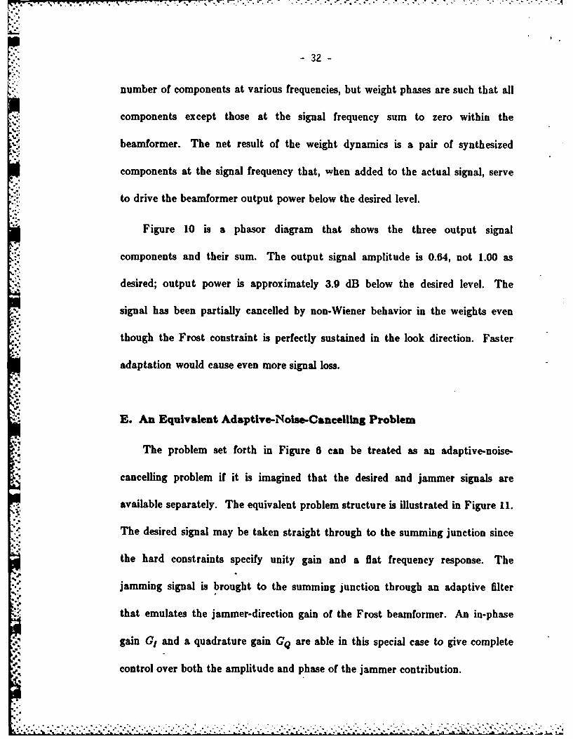
E. An Equivalent Adaptive-Noise-Cancelling Problem

The problem set forth in Figure 6 can be treated as an adaptive-noise-

cancelling problem if it is imagined that the desired and jammer signals are

available separately. The equivalent problem structure is illustrated in Figure 11.

The desired signal may be taken straight through to the summing junction since

the hard constraints specify unity gain and a flat frequency response. The

jamming signal is brought to the summing junction through an adaptive filter

that emulates the jammer-direction gain of the Frost beamformer. An in-phase

gain G1 and a quadrature gain GQ are able in this special case to give complete

control over both the amplitude and phase of the jammer contribution.

-iE--

CD 4-T

C-)-

E

C4-

CD

4 I-

* CD

-jA

-34-

CL

4 4J

'A-U-

V.' 4-)

U-

C)~

L

'-

4-.)

St . .7. 7 . .

-35-

Expressions relating G, and GQ to the ABF weights w 1, w 2, w 3, and w 4

are needed to complete the specification of the equivalent problem. The required

expressions may be derived from the equation for the jammer output from the

ABF:

Yt) w 1 cos WJt + w 2 cos(kwjt-0ce) + w3 sin wJt + w 4 sin(wjt-ee)

(2-31)

where 0,, is the element-to-element phase delay for the jammer signal. After

making use of trigonometric identities and regrouping terms, the equation

becomes

YO j)= [w I + (cos 0,,)W2-(sin 0J)w 4] cos wjt

+ (sin 0,,)w2 + w 3 + (cos 0ee)WJ sin wjt . (2-32)

Comparison of this equation with the structure of Figure 11 yields the

relationships

=-- -[w + (cos ec )w2 -(sin 0,, )w J (2-33)

GQ = -[(sin0,)w 2 + w3 + (cos 0,e)W

, The equivalent system involving G and GQ allows a considerably simpler

* characterization of the weight dynamics associated with signal cancellation than

would have been possible in the four-dimensional weight space of the original

problem. In particular, the reduced dimensionality simplifies comparisons of the

dynamic solution obtained during cancellation with the Wiener solution that is

approached at low adaptation rates.

- 36 -

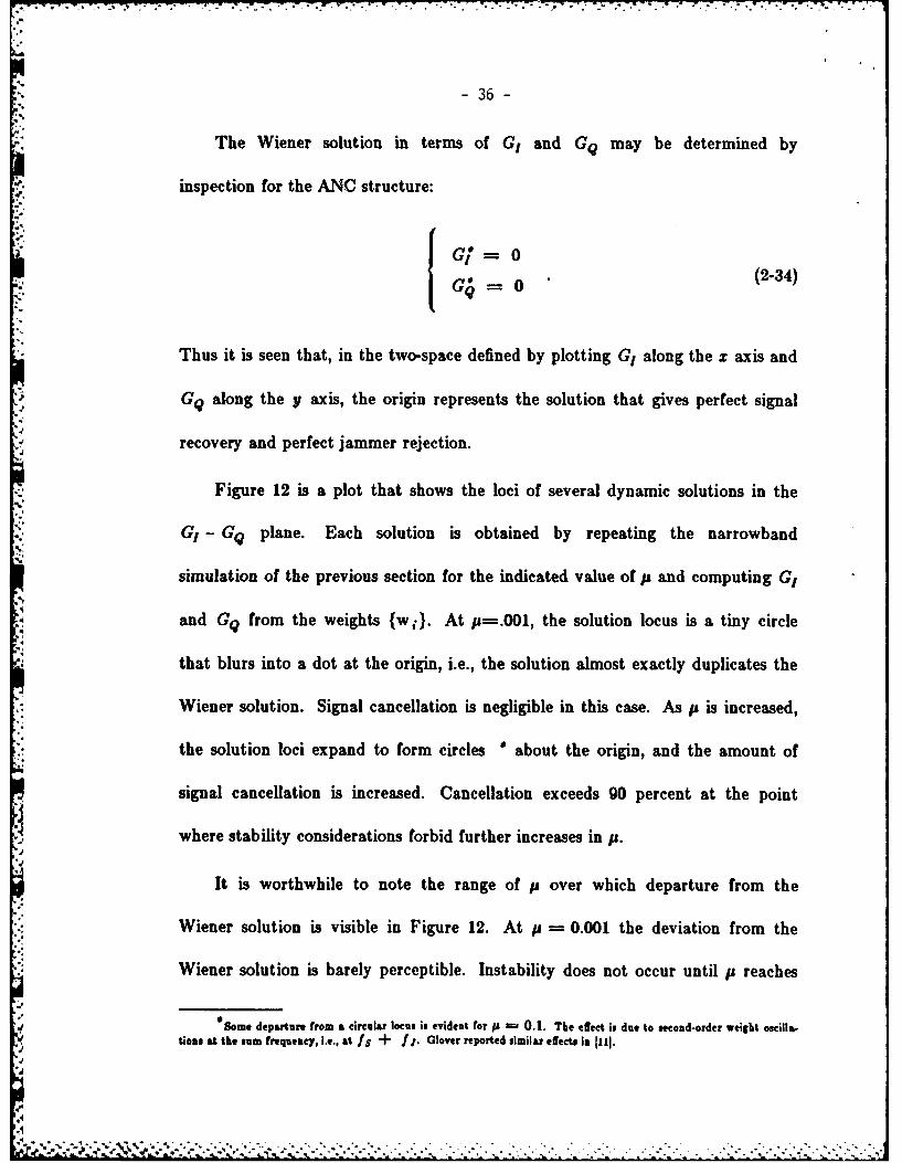
The Wiener solution in terms of G i and GQ may be determined by

inspection for the ANC structure:

SG/= 0. 0 (2-34)

Thus it is seen that, in the two-space defined by plotting G, along the z axis and

GQ along the y axis, the origin represents the solution that gives perfect signal.

recovery and perfect jammer rejection.

Figure 12 is a plot that shows the loci of several dynamic solutions in the

G, - GQ plane. Each solution is obtained by repeating the narrowband

simulation of the previous section for the indicated value of pU and computing G,

and GQ from the weights {w }. At p=.OO1, the solution locus is a tiny circle

that blurs into a dot at the origin, i.e., the solution almost exactly duplicates the

Wiener solution. Signal cancellation is negligible in this case. As p is increased,

the solution loci expand to form circles " about the origin, and the amount of

signal cancellation is increased. Cancellation exceeds 90 percent at the point

where stability considerations forbid further increases in p.

It is worthwhile to note the range of p over which departure from the

Wiener solution is visible in Figure 12. At p= 0.001 the deviation from the

Wiener solution is barely perceptible. Instability does not occur until p reaches

Some departure from a circular locus is evident for j -A 0.1. The effect is due to second-order weight oscilla-tioas at the sum frequency, i.e., at fS + f 1. Glover reported similar effects in Jllj.

%,4

J

-37-

'S1 .0

.4IMI = 0. 9

.0.

bM) = M) istemantdeo0h

mi.0 dus0en

FigureM0. 120ouio-oiinte0GQPae

CO0511 . .

-38-

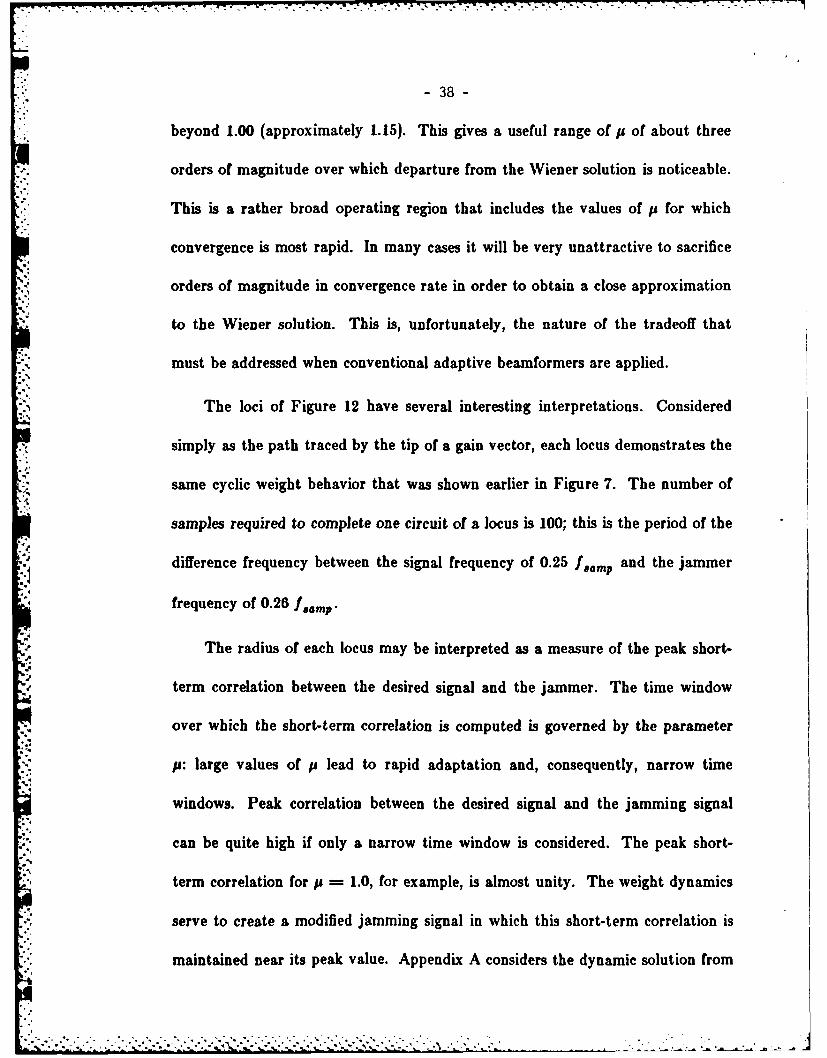
beyond 1.00 (approximately 1.15). This gives a useful range of p of about three

orders of magnitude over which departure from the Wiener solution is noticeable.

This is a rather broad operating region that includes the values of p for which

convergence is most rapid. In many cases it will be very unattractive to sacrifice

orders of magnitude in convergence rate in order to obtain a close approximation

to the Wiener solution. This is, unfortunately, the nature of the tradeoff that

must be addressed when conventional adaptive beamformers are applied.

The loci of Figure 12 have several interesting interpretations. Considered

simply as the path traced by the tip of a gain vector, each locus demonstrates the

same cyclic weight behavior that was shown earlier in Figure 7. The number of

samples required to complete one circuit of a locus is 100; this is the period of the

difference frequency between the signal frequency of 0.25 empand the jammer

frequency of 0.28 am

The radius of each locus may be interpreted as a measure of the peak short-

d term correlation between the desired signal and the jammer. The time window

over which the short-term correlation is computed is governed by the parameter

p: large values of p lead to rapid adaptation and, consequently, narrow time

windows. Peak correlation between the desired signal and the jamming signal

can be quite high if only a narrow time window is considered. The peak short-

term correlation for p = 1.0, for example, is almost unity. The weight dynamics

serve to create a modified jamming signal in which this short-term correlation is

maintained near its peak value. Appendix A considers the dynamic solution from

- 39 -

the viewpoint of short-term correlations and develops a closed-form description of

weight behavior when both signal and jammer are sinusoidal.

Another way to view the loci of Figure 12 is to treat them as traces of the

minima of dynamic error surfaces. It is well known that, in the stationary case,

the Wiener solution defines the minimum of a quadratic error surface. In the

case at hand, the error surface may be treated as static only at small values of p.

-9 The minimum of the surface in the stationary case is not at zero error, but is

elevated above zero by the power level of the desired signal. At low values of p

the Wiener solution is closely approximated, and the desired signal is delivered

essentially without loss at the beamformer output. As p is increased, the error

surface must be treated as dynamic. The minimum of the error surface no longer

coincides with the Wiener solution. Instead, for the simple case under

consideration, the minimum lies on a circle centered on the Wiener solution.

Furthermore, the dynamic minimum does not lie at the same error level as the

Wiener solution. The elevation of the minimum is decreased by the amount of

* signal cancellation attainable at a given value of p. The decrease, expressed as a

fraction of the desired signal power, is related to the quantity termed

miaadjustment 131

misadjustment = M(p) A El12(tLl-El(y*(flt (2-35)E[(y *(t))g 2-5

where y*(t) is the output with the optimal weight vector W*. Because E[y 2(t)]

is less than E(V*(t))21, misadjustment is a negative quantity in the region of

,,a ,., ' -. . ., . - ,, . - . . . . , .. - .. . . . .- , - - .. .- -. . . , - . . • , ,.4 - -d - I . . . i

40-

interest. It is, however, the magnitude of misadjustment that is important, not

the sign. The contours of Figure 12 have been labelled to show I M(p) I levels as

well as p values.

The discussion of the error surface that has just been given differs somewhat

from earlier treatments. For a given ABF structure, the error surface has

previously been considered simply as a function of the input signals; changes in

the error surface were attributable to changes in the input signal description.

Here the error surface has been described as a function of the adaptation

parameter. In other words, the error surface must be described in terms of the

signal environment perceived by the beamformer, not simply in terms of some

detached statistical characterization of the incident signals.

The view of the solution set that has just been given indicates the nature of

the problem at hand. There is a direct coupling between the adaptation

parameter that is chosen and the solution that is delivered by the ABF. Low

values of the adaptation parameter p yield a solution that conforms closely to the

Wiener solution and satisfies the requirement for signal preservation. These

values of p fail, however, to meet the requirements of responding rapidly and

tracking a dynamic signal environment. Higher values of p provide better

tracking of changes in the environment, but the non-Wiener solutions involve

sacrifices in the quality of the recovered signal. Given the beamformer under

consideration, nothing can be done beyond striking the best compromise between

signal q,3ality and tracking capability. A change in the nature of the beamformer

'. .

- r'flr7r~ rn r r r - r r -

- 41 -

is needed to break away from the limitatioDs imposed by the coupling between

the adaptation parameter and the solution generated by the ABF.

I

-,*1%4

.5

.1

'4

*~

.5.4

.54

II

*4~* 4.. .....-.....-*.' . - -~ ~ - - <a. ~ -* S -~~~*~>' ~ 4.~ a .Z.tL>.L.t.A.

-42-

MII. A COMPOSITE BEAMFORMER THAT ELIMINATES SIGNAL

CANCELLATION

Chapter 2 has illustrated the signal cancellation effects that can arise in

relatively simple signal/jammer scenarios and has demonstrated that even the

most rigid constraints can fail to preserve the desired signal. This chapter turns

from a discussion of the problem to the description of a solution and shows how

signal cancellation can be avoided at the price of some increase in beamformer

complexity.

Chapter 3 consists of three sections. The first section builds upon the

background provided by Chapter 2 and reformulates the adaptive beamformer

.* problem in such a way that jammer nulling can be accomplished at high

adaptation rates without signal cancellation. The beamformer structure that

arises out of the reformulation is termed a composite beamnormer or CBF. The

next section discusses the key issue of signal relationships within the new

beamformer. A demonstration of the performance improvement afforded by the

new beamformer is given in the third section by revisiting the wideband problem

from Chapter 2.

A. Problem Reformulation

Chapter 2 and Appendix A described the differing solutions derived by a

hard-constrained beamformer at various adaptation rates. The solutions differ

.. . . . . . . . . . . . . . .:,,,-,'....,,..,:.:,,:,..... , .. :-:,. .- ::...: ... .-. ;.....-. .. .... .-........... .... .. ,

.- 1 -7 71 -

-43

-43because, from the beamformer viewpoint, the problem changes. Unfortunately,

the viewpoints of the beamformer and the system designer begin to clash as

signal cancellation becomes significant. The designer is not interested in the

minimization of output power at all costs, and will typically invoke constraints in

an attempt to restrict the minimization process. The beamformer, however, is

designed to relentlessly pursue minimization. At high adaptation rates the

beamformer weights possess the mobility to exploit short-term correlations

between signal and jammers and thereby circumvent the constraints. Design

objectives are simultaneously bypassed, and system performance is

unsatisfactory. A problem reformulation is needed that harmonizes design

objectives with the realities of beamformer behavior at high adaptation rates; this

section pursues that reformulation.

Two observations can be made at this point that are useful in developing a

problem reformulation. One observation is that interaction between the desired

signal and the jammer is the root of the cancellation phenomenon. The nature of

this interaction was demonstrated in some detail in Chapter 2 for the case

involving a signal and a jammer that are narrowband. It was shown-4

experimentally and analytically that the presence of both signal and jammer

energy is a prerequisite for signal cancellation. In particular, it was shown that

" the output signal is the "target" of the cancellation process and that short-term

correlation between signal and jammer waveforms is the phenomenon that makes

*: cancellation possible.

-44-

A second observation that can be made is that the signal plays no role in the

Wiener-solution calculation in a perfectly steered Frost ABF. In other words, it

is completely equivalent to write

wO = RfJlCICTRjvCl (3-1)

rather than the earlier statement

Ws R 1C[C T R-j C] I , (2-13)

where RXX = Rss + RNN as originally assumed. This point can be appreciated

- intuitively from the fact that the look-direction response is determined

exclusively by the hard constraints, not by the desired signal. The equivalence of

(3-1) and (2-13) may be rigorously demonstrated by substituting for R in (2-

13) and simplifying. An appropriate substitution is

RXX = Rss + RNN = CT RRR C + RNN (3-2)

where RRR is the autocorrelation matrix for the vector of signal voltages

appearing at the taps of any one of the beamformer filters. Appendix B traces

the somewhat lengthy proof of the equivalence for both a narrowband processor

using a single complex weight per beamformer channel and a wideband processor

using tapped-delay-line filters for each beamformer channel. Yet another way to

explore the role of the signal is to consider the problem in the context of an

equivalent generalized sidelobe canceller; Appendix C discusses this approach to

the problem.

.45

- 45 -

Reconsideration of the adaptive beamformer problem has thus far indicated

1) that the signal drives the process of signal cancellation that results in its own

demise and 2) that the signal has no role in the determination of a set of weights

that optimizes array performance. These two points argue for exclusion of the

desired signal from the beamformer. The overlooked consideration is, of course,

that the original objective was to recover the signal. The remaining step is to

harmonize the objectives of cancellation-free adaptation and successful signal

. reception by devising a structure that excludes the signal from the adaptive

process but allows the signal to pass through to the system output. The problem

reformulation thus amounts to more precisely defining the role of the desired

signal in an adaptive array.

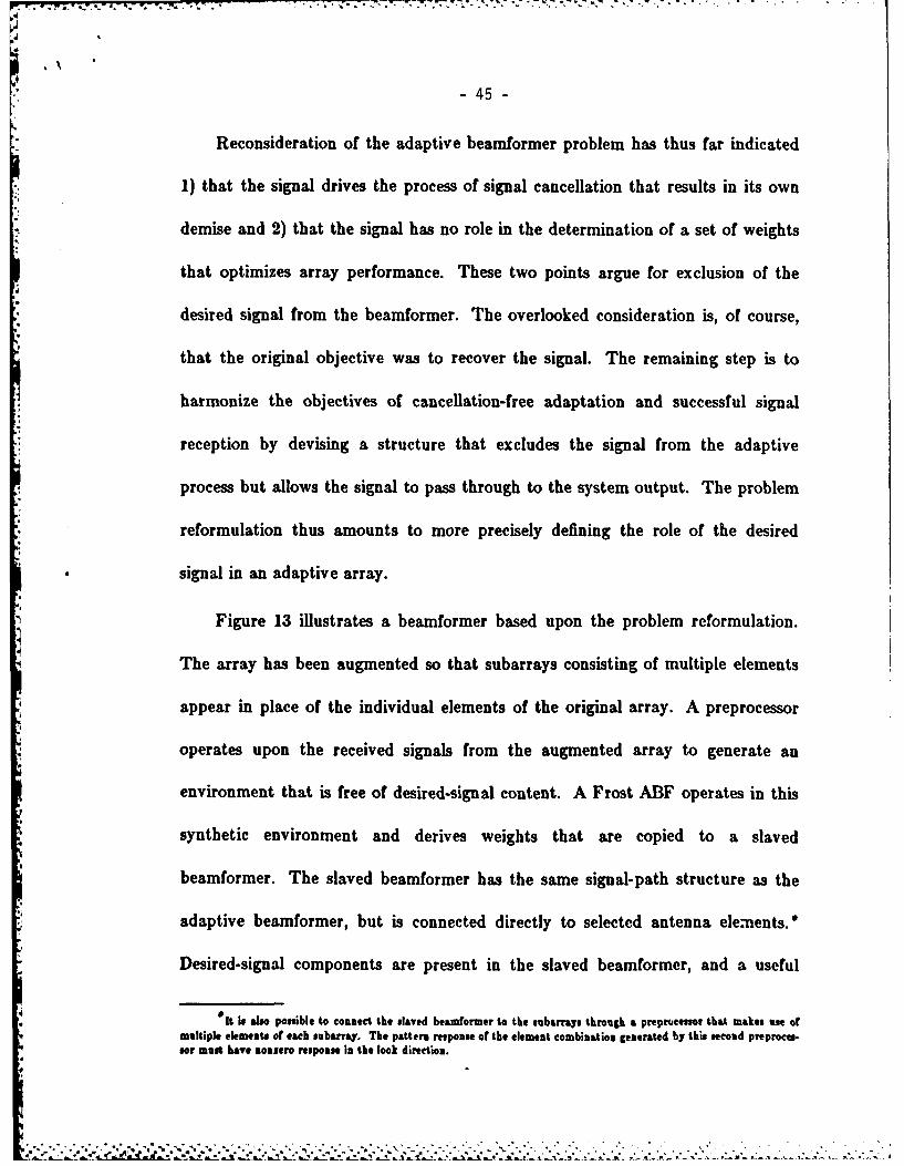
Figure 13 illustrates a beamformer based upon the problem reformulation.

The array has been augmented so that subarrays consisting of multiple elements

appear in place of the individual elements of the original array. A preprocessor

operates upon the received signals from the augmented array to generate an

environment that is free of desired-signal content. A Frost ABF operates in this

synthetic environment and derives weights that are copied to a slaved

beamformer. The slaved beamformer has the same signal-path structure as the

adaptive beamformer, but is connected directly to selected antenna elements.*

Desired-signal components are present in the slaved beamformer, and a useful

*It is also possible to connect the slaved beamformer to the subarrays through a preprocessor that makes ase ofmultiple elements of each subarray. The pattern response of the element combination generated by this second preproca.sor must have nonsero response in the look direction.

• -4 .. -.. ' . ' " ' -. -'- -. -. . ' ,-"- ' -'- " ? ' . .i i ..i .• .

- 771-. .- 7 71

-46-

I I.-

4.>.

tu I

4.-

4.L

- I-

0L

coLL

44

(n4

.4' LL-

%! j

-47

output may be drawn from it.

Taken as a whole, the structure shown in Figure 13 is termed a compo8ite

beamformer (CBF). The key elements are 1) an augmented array, 2) a

preprocessor that excludes the desired signal from the adaptive process, 3) an

2 adaptive beamformer that can be constrained to control look-direction response

while nulling jamming signals, and 4) a slaved beamformer that is used to

implement the computed solution and recover the desired signal. Three of these

elements, the array, the preprocessor and the adaptive beamformer, afford

considerable flexibility in that a variety of specific realizations are possible; the

I slaved beamformer design is inflexible in the sense that it mirrors the adaptive

beamformer design. Appendix D describes an alternative CBF realization based

Vupon Widrow's pilot-signal algorithm; other realizations may also be derived.

B. Signal Relationships in the CBF Master and Slave

Because CBF operation involves the derivation of weights in the master

beamformer for application in the slave, it is essential that the signal sets in the

two beamformers be closely related. Ideally, the two signal sets would be

identical, save for the absence of look-direction components in the master. This

would assure that weights derived in the master were equally appropriate for and

effective in the slave. Unfortunately, it is not possible, in general, to attain the

ideal signal relationships between the two beamformers, and compromises must

be allowed. This section begins a discussion of the nature of the compromises

."4. - .. , . .' , . . . . . . , - - . - . . - - . . .. ,- . . . . . . . - . . . .. . . .

*1 . I .kdl - ... --... = a- '- .d .I.. -.-- - -,-- - .- - .

I

-48-

that are necessary and of the consequences of those compromises.

The basic difficulty in attaining the ideal signal sets lies in removing the

* look-direction signal from the master beamformer without perturbing the various

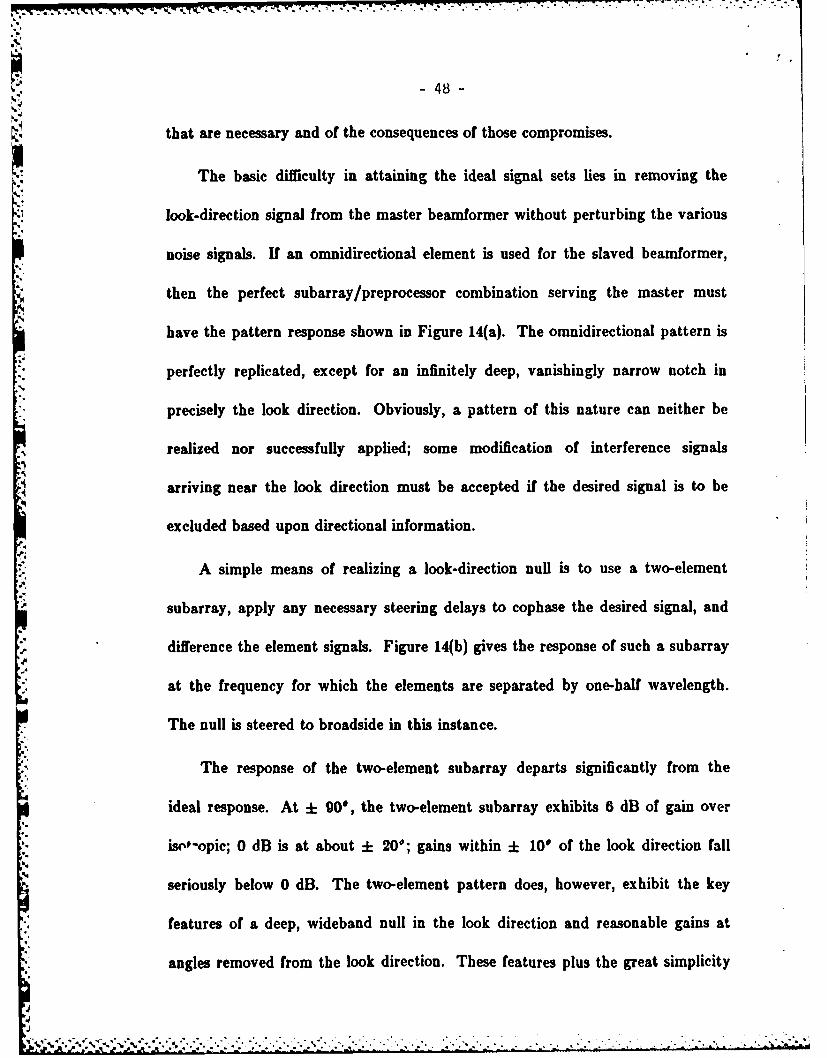
noise signals. If an omnidirectional element is used for the slaved beamformer,

then the perfect subarray/preprocessor combination serving the master must

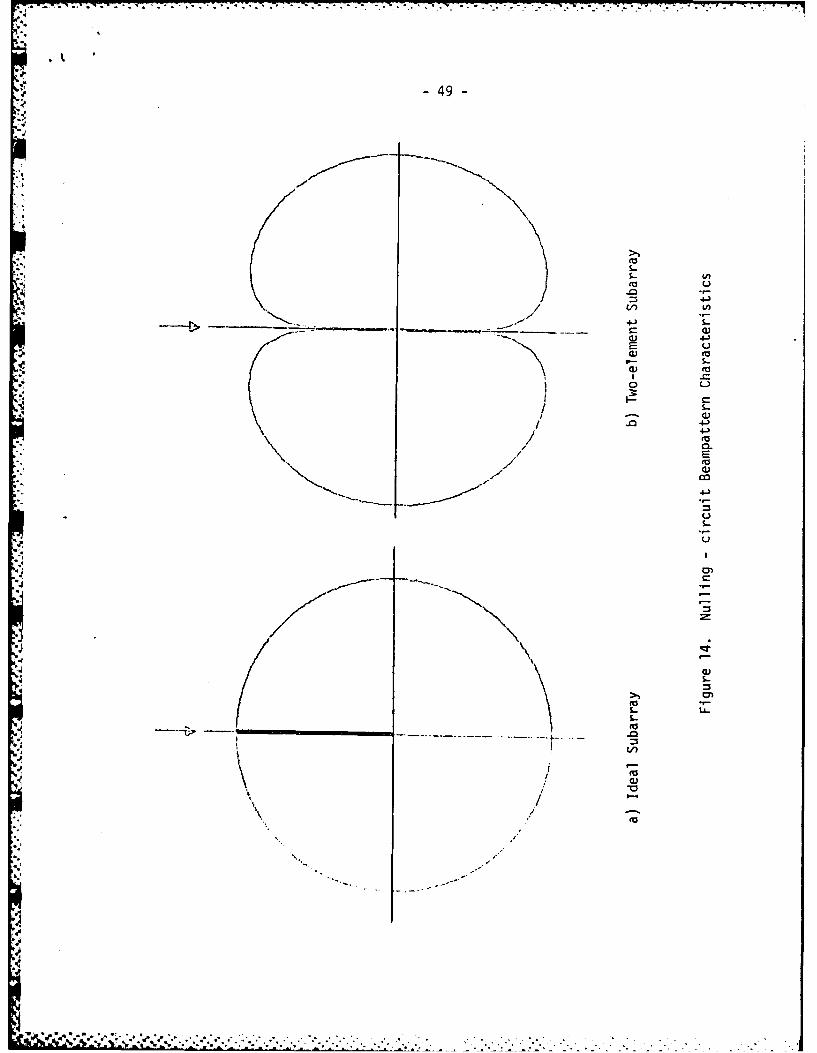
have the pattern response shown in Figure 14(a). The omnidirectional pattern is

perfectly replicated, except for an infinitely deep, vanishingly narrow notch in

precisely the look direction. Obviously, a pattern of this nature can neither be

realized nor successfully applied; some modification of interference signals

arriving near the look direction must be accepted if the desired signal is to be

excluded based upon directional information.

A simple means of realizing a look-direction null is to use a two-element

subarray, apply any necessary steering delays to cophase the desired signal, and

difference the element signals. Figure 14(b) gives the response of such a subarray

at the frequency for which the elements are separated by one-half wavelength.

The null is steered to broadside in this instance.

The response of the two-element subarray departs significantly from the

ideal response. At E o90., the two-element subarray exhibits 6 dB of gain over

is- "opic; 0 dB is at about ± 20'; gains within ± 10. of the look direction fall

seriously below 0 dB. The two-element pattern does, however, exhibit the key

features of a deep, wideband null in the look direction and reasonable gains at

angles removed from the look direction. These features plus the great simplicity

4d

-- 49

*14J

- S-

-~ 0)

E E

I -J

o. LL.I-

UP to~ .

-50-

of the subarray/preprocessor make the two-element subarray worthy of more

detailed consideration.

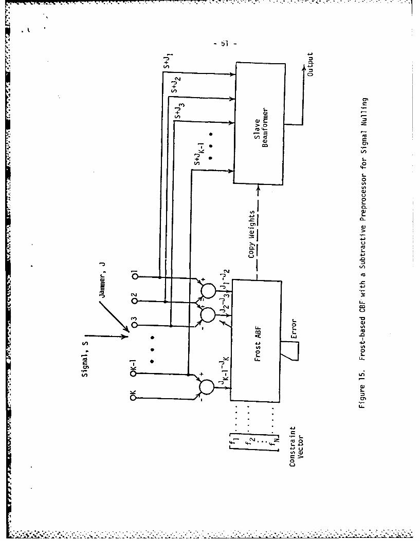
The general CBF structure of Figure 13 may be specialized to yield the CBF

shown in Figure 15. Here the desired signal is assumed to be incident from

broadside so beam steering may be neglected. The preprocessor is realized by

using two-element subarrays in a simple element-differencing scheme. The

sharing of elements between subarrays provides very efficient use of elements;

only a single element is needed beyond those ordinarily required for a comparable

array.

A Frost ABF operates upon the preprocessor output to derive a set of

weights that minimizes error power subject to a set of look-direct constraints. It

should be noted that, in contrast to conventional adaptive beamformers, the error

power is distinct from the CBF output signal power. Error power can be driven

to zero without endangering the desired signal component in the output. This is,

in fact, the ideal state of affairs.

Because weights derived in the Frost ABF will be applied in the slaved

beamformer, it is vital that relative signal phases match in the two beamformers.

The uniform structure that exists in the preprocessor assures that this phase

matching will be obtained. The set of two-element subarrays feeding the Frost

ABF echoes the structure of the array of omnidirectional elements serving the

°Element sharing among subarrays does introduce thermal-noise correlations in the master beamformer that are

not present in the slave. Generally, however, thermal noise powers will be relatively low, and these spurious correlationswill not seriously affect performance.

> 0

CZ

VI 0'4-

0V)(UL)0S..

C0.

4-3

oo

cn 4.)

0.

a)7

L.

C.-

SS

*~ (Z o

= . . .. . .-,S , -. _... * ---. .-- - , .- . .-*' -. .,.

-52-

slaved beamformer.

Phase relationships between signals in the ABF and the slaved beamformers

are made clearer in Figure 16. The jammer components received by the

omnidirectional elements are indicated by a set of equal-amplitude, uniformly

spaced phasors J1, J2 , J3 , ... , JK-i, JK" The preprocessor operates upon these

inputs to produce the phasor outputs JI-J 2, J2-J3 , ..., and JKI-JK. These

phasors are also equal in amplitude and have the same phase-angle separations as

the received jammer components. The preservation of relative phase in the

preprocessor assures that weights that generate a null in the ABF will also

generate a null in the slaved beamformer.

The phasor argument as advanced in Figure 16 applies to a single jammer at

a single frequency. Linearity and superposition apply, however, and show that

phase relationships are preserved for multiple jammers and for broadband as well

as narrowband signals.

The uniform linear array provides an attractive structure for the CBF

-' because there is the option of element sharing between subarrays. A regular

array structure is not, however, a prerequisite for the CBF. The fundamental

requirement is for phase matching between the master and slave beamformers.

Phase matching may be obtained for an arbitrary array geometry by augmenting

each original element to form identical subarrays at the element locations.

Identical preprocessors may then be used to form subarray responses with nulls in

the selected look direction. The preprocessor outputs must be cophased for the

4.; ' , :,.,,, , ,, -, ' .- ,.-. , ' ,, '. , ' ., - . . ,- . . .- - - , -i i- . , ,.--i , " : .- - - -

-4-

-4-

LL.

cLii

5-,

4 -

0

4~

- 54 -

look direction and applied to the adaptive beamformer while the original element

outputs are cophased and applied to the slave.

C. CBF Performance - An Example

The CBF described in the previous section is capable of delivering much

better performance at high adaptation speeds than, say, a comparable Frost

ABF. The performance contrast may be conveniently illustrated by returning to

the wideband problem of Chapter 2 for which the Frost ABF performance has

already been demonstrated.

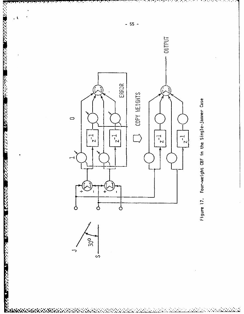
Figure 17 diagrams the wideband problem with a Frost-based CBF replacing

the original Frost ABF. The signal and jammer descriptions are identical, as are

the look-direction constraints. A third antenna element has been added in order

to provide appropriate inputs for the subtractive preprocessor. Two of the

]. elements also serve the slaved beamformer, which makes use of weights from and

functions in parallel with the adaptive beamformer.

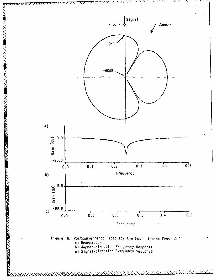
. The antenna pattern at the jammer frequency of 0.25 feamp is shown in Part-;..%

: 'i a) of Figure 18. This plot was generated after initial transients had died away

and jammer nulling was essentially complete. A deep notch exists at the jammer

arrival angle of 301.

Parts b) and c) of Figure 18 show the frequency response in the jammer

direction and look direction. The jammer-direction plot reveals a deep notch at

the jammer frequency. The look-direction plot confirms that the unit-gain, all-

',S ,, , ,. . ."." • • ", . -. .-. . - - - .... ,. . ',. - .. , .',. , . r ., - '. -.- ' '- ,. .,- , - . - .",- , . . ..

-55-

C-F-

cxcD

-pU

LLGJ

CDC

r )

S.-

ca

Signal-56 -ir Jammer

:, OdB

-60dB

a.a

C

,C

-80.0 ___________________________

0.0 0.1 0.2 0.3 0.4 0.5

.4*1b) Frequency

-oSo

~1 0.0.1

C

C) 80.0

0.0 0.1 0.2 0.3 0.4 5

Frequency

Figure 18. Postconvergencc Plots for the Four-elern.ent Frost ABF

a) Beampatternb) Jamer-direction Frequency Responsec) Signal-direction Frequency Response

.p.. S -IS~I- '

-57-

pass response specified by the constraints has been attained.

Some of the contrasts between Frost ABF and CBF performances may be

seen by comparing Figure 3 and Figure 18. The notch depths in both Part a)

and Part b) of the figures are greater for the CBF than for the Frost ABF, thus

indicating improved jammer rejection.47

A more dramatic view of the performance contrasts is provided by the

spectral plots of Figure 19. Parts a) and b) of the figure show ensemble averages

of the desired signal spectrum and the jammer spectrum. Part c) repeats the

ensemble-averaged Frost output spectrum that was shown in Figure 4. Part d)

provides the ensemble-averaged CBF output spectrum. The signal-cancellation

effects seen in Part c) are not present in the CBF spectrum, and extremely close

matching with the desired-signal spectrum is evident.

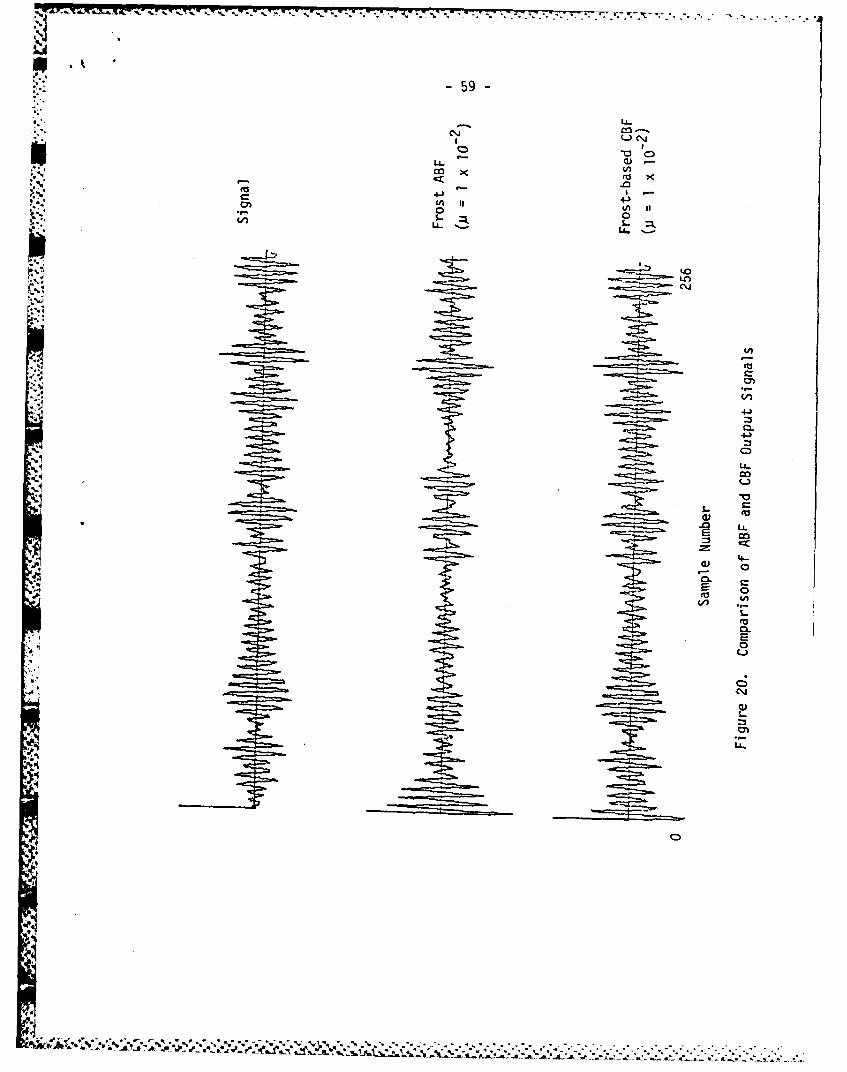
The differences between Frost ABF and CBF performance may also be

clearly seen in the time domain. Figure 20 contains 256-sample segments of time

domain data taken from the beginning of the simulation. Part a) illustrates the

desired-signal waveform; Part b) the Frost-ABF output; and Part c) the CBF

output. Both output waveforms show the transient associated with jammer

nuiling. Nulling should be complete within 50 samples, and good tracking of the

desired signal should be seen. The Frost-ABF output, however, shows

considerable distortion due to signal cancellation. CBF tracking, on the other

hand, is essentially perfect after jammer nulling.

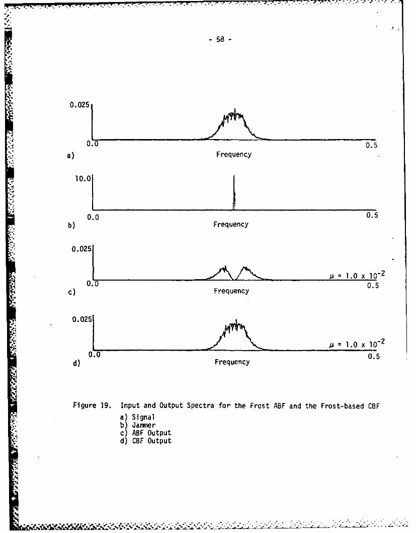
- 58 -F

0.025

0.00.5

a) Frequency

10.0

0.0 0.5b) Frequency

a'i 0.025

0.- . "_ ujj 1.0 x I 0-2

C) Frequency 0.5

0.025

ju = 1.0 x 1.0-2

0.0 0.5

d) Frequency

Figure 19. Input and Output Spectra for the Frost ABF and the Frost-based CBF

a) Signalb) Jammerc) ABF Outputd) CBF Output

-59-

< .0

0(A Ln

L.6

LO.

-V.-

LA

IF0

- 60 -

IV. PERFORMANCE OF THE COMPOSITE BEAMFORMER

The preceding chapter introduced the composite beamformer (CBF) and

illustrated the performance of a particular CBF realization based upon a simple

subtractive preprocessor and Frost's constrained LMS algorithm. An argument

I was advanced that, due to the deliberate phase matching between the master and

slave beamformers, jammer nulling is quite good in the CBF. Additionally, signal

cancellation of the type that can be so destructive in a hard-constrained ABF is

effectively suppressed. A sample case was shown in which the expected

improvements over a Frost ABF were, in fact, realized by a CBF using a simple

signal-nulling scheme.

This chapter continues the exploration of CBF performance. The first

., section examines the issue of CBF optimality in greater depth. The second

section then describes further simulation experiments designed explicitly to probe

CBF behavior with regard to optimality. A third section considers convergence

time constants in the CBF and draws comparisons with the Frost ABF. The

* fourth section describes CBF weight behavior near convergence and shows

contrasts between CBF and ABF behavior in that important region.

..

A. CBF Optimality In the Narrowband Case

The experiment of the previous chapter has indicated that, at least in a

selected case, the performance of the CBF at high adaptation speeds is greatly

superior to that of a comparable ABF. Questions remain, however, about the

I!

-61-

range of conditions for which optimal performance is approached. In this section

the issue of optimality will be investigated in greater depth for the important

case in which jammer signals are narrowband.

The discussion in this section will center upon the noise autocorrelation

matrix RNN. As was shown in Chapter M, R - governs the optimallolution for

the Frost ABF. Ideally, the adaptive (master) processor in the CBF would

receive unperturbed noise voltages and would thus tend toward the optimal

solution as indicated by Rjv. In practice, the phases of interference signals are

preserved through appropriate preprocessor design, but the interference

amplitudes (or, equivalently, the interference-to-thermal-noise ratios) are altered.

It is of interest to consider the influence of perturbations in interference-to-

thermal-noise ratio upon R -1

The signal vector u, associated with the itA narrowband interference source

may be written as

~e i #2'

= f(O,Pi)x = f(Oi,Pi) (4-1)

where f (i,Pi) is the pattern response of the K identical elements (or subarrays)

constituting the array, ei is the arrival angle of the signal with respect to a

reference direction, Pi is the signal power, ji is a propagation vector, and 01i is

the signal phase at the 1tA element with respect to a coordinate origin. For the

!6A .I * . . . .

IM It.-62-

important case of a uniform linear array with element spacing d, (4-1) may be

specialized to

1

Le:1 4, = f(O,,P,) " (4-2)

where the first element is taken as the phase reference and

- 27r(-) sin O, (4-3)

,x i

,* is the element-to-element phase shift for an arrival angle 9, (measured clockwise

from array broadside) and an interference wavelength of Xj.

Pattern responses of two types will be of interest. For an ideal

omnidirectional element,

f 1(P) = ei • (4-4)

If two such elements are placed a half wavelength apart and their outputs are

differenced to form the simple nullformer discussed previous!y, then

f 20A) = Pi[2 - 2 cos(v sin 0)] (4-5)

The noise autocorrelation matrix RNN for a K-element narrowband array

Itakes a simple form under the assumptions that the thermal noise voltages from

the elements are zero-mean Gaussian and mutually uncorrelated and that the M

incident narrowband signals have carrier phases that are uniformly distributed on

U - - -e

63-

(0,2r) and statistically independent both of one another and of the thermal noises

of the elements. Specifically,

MRNN = [1+ Pi .1C 47 2 , (4-6)~i,-I

where I is the K X K identity matrix, pi is the power ratio between the Ok

interference signal and the thermal noise voltage, and a2 is the thermal noise

variance. The power ratio pi incorporates the pattern response f (Oi,P,) and 2

ii ! (o ,p,)f ppl--i. o(4-7)

.p." Gupta and Ksienski [20] have observed that correlation matrices having the

structure of (4-6) may be inverted into a convenient form when the matrices are

'.4 reexpressed in terms of an orthonormal basis for {. }. Their method will be used

to derive an expression for R- 1 . This expression will then be used to determine

conditions under which the CBF solution approaches that of the Frost ABF.

The Gram-Schmidt process may be applied to construct an orthonormal

basis {g.}, i=1, 2, ..., M, for the {.}), i=1, 2, ... , M. As a preliminary step the

first basis vector is computed:

-,"lTe (4-8)

Then a set of orthogonal vectors {jU.}, i=1, 2, ... , M, is determined from

",,

-64-

.1,

i! "

- N r~i) i(4-9)

i-I

and normalized according to

0if~T e 0,. , -- (4-10)

otherwise

The vectors {l, may now be written in terms of the basis vectors. The

expression given in (4-0) may be rearranged to yield

i-!=- 1 - .0i + ., (4-11)

Forming the transpose in (4-11) and postmultiplying by u. then gives

AT = AT -C = VJO AT = A*(12

where the orthonormality of {.} has been used to simplify the expressions. By

using (4-11) and (4-12) together with the definition

*l 4iT (4-13)

-X. may be written as

i- = X~ (4-14)* j.i

The expression (4-6) for RNN now becomes

. % * ° o . ° -. - ' . " • • .. - . , . - o. ' °.. . . . . . . . . . . . .. ' . .-o .o ° .' .. °'° " - -. "" ' ..

- 5 -

M ),RNN ={I+ EPi Rile I ak ]r (4-1)

Because the optimal weights for both the Frost ABF and the Frost-based CBF

depend upon R-, it is necessary to invert the expression on the right-hand side

of (4-15). The inversion technique depends upon the matrix inversion lemma*

and is most readily applied by first considering the case M 1. In that case

(4-15) becomes

RNN = (I +1 p l 1 . } 2 (4-16)

Application of the inversion lemma to (4-16) then yields

R - p1 2 12(I + a T p, a 2 )-'1 } V -T (4-17)

which rearranges to the form

R = I1- (4-18)f +.0~2

By orthonormality,

Te

Also

The lemma is discussed in Appendix B in wother context.

- . . . . . . .. -F -. . . .-. . ---.

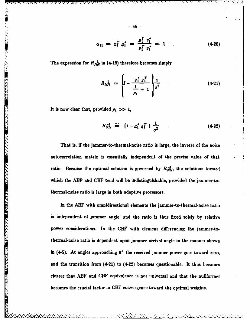
7;.. -Z 7 .. - -N

I.I

- 66 -

T =, =. (4-20)

The expression for RJv in (4-18) therefore becomes simply

R-1_ 1-_14 (4-21)

It is now clear that, provided Pi >> 1,

NNv - (I-.g g } 1" (4-22)

That is, if the jammer-to-thermal-noise ratio is large, the inverse of the noise

autocorrelation matrix is essentially independent of the precise value of that

ratio. Because the optimal solution is governed by RRN, the solutions toward

which the ABF and CBF tend will be indistinguishable, provided the jammer-to-

thermal-noise ratio is large in both adaptive processors.

In the ABF with omnidirectional elements the jammer-to-thermal-noise ratio

is independent of jammer angle, and the ratio is thus fixed solely by relative

power considerations. In the CBF with element differencing the jammer-to-

thermal-noise ratio is dependent upon jammer arrival angle in the manner shown

in (4-5). At angles approaching 00 the received jammer power goes toward zero,

and the transition from (4-21) to (4-22) becomes questionable. It thus becomes

clearer that ABF and CBF equivalence is not universal and that the nuilformer

becomes the crucial factor in CBF convergence toward the optimal weights.

,,. .

- 67 -

If consideration is now given to the two-jammer case (4-15) becomes

RNN = (I + plaft1g141 + P2f4laaT9 + P2c*20fMA19. , + ,,, ,.1 + p2& , } . (4-23)

Repeated application of the matrix inversion lemma shows that

eT

RNg IV2 (4-24)

1 p2a2

Again, under the assumption that P2 > 1, i.e., that the power of the second

jammer is well above the noise and that the projection of the second jammer's

propagation vector onto the second basis vector is nonzero

1 2 02! - - 1 ; ; . (4-25)

This expression is, like (4-22), independent of the jammer-to-thermal-noise ratios

under the assumptions stated; it follows that the ABF and CBF solutions are

again equivalent.

If the methods and assumptions just described for the single-jammer and

dual-jammer cases are extended to the case of M jammers, then

NN (I1 + (4-26)iII

That is, the ABF and CBF solutions become indistinguishable for the cases where

jammer-to-thermal-noise ratios in the adaptive processors remain large.

-68-

Two conditions must be satisfied for the jammer-to-thermal-noise ratio in

the CBF to be large. In the first place, of course, the jammer signal must arrive

at the array elements with appreciable power. This will usually be the case if the

jammer constitutes a threat. A second condition is that the nulformer not

discard so much jammer energy that the jammer contribution is driven into the

thermal noise. In the case of the two-element subarray, this difficulty may arise

at angles near the look direction, i.e., within about 10. of the signal azimuth;

with other nullformers the regions that seriously attenuate jammer signals may

be different.

A third condition must also be satisfied if the CBF weights are to reliably

approach optimality. This last condition relates to the number of degrees of

freedom available versus the number of jammers that must be nulled. In the

narrowband case one complex weight is adequate to null a jammer. If there are

*K beamformer channels, then the number of jammers must be less than or equal

to K-1 since one complex weight is lost to the constraints in a narrowband Frost

ABF.

B. Further Simulation Experiments with the CBF

Two additional simulation experiments were devised to assess CBF

performance under more difficult conditions than the single-jammer scenario of

Chapter 3. Particular attention was given to testing the optimality criteria just

discussed.

g * *. . U? * * **.. .. : . ,- '.: -:-"- -:- . * - .?- * - .. '". .-.-..-:- . .... - . -. _. -

-69-

The signal/jammer scenario for one experiment is shown in Figure 21. The

CBF configuration is identical to that used in the experiment of Chapter 3, but

the jammer environment has been altered. The jammer Jn is a signal centered at

0.25 learp with a bandwidth of 1%. The actual power of J, is 2.0, and its

arrival angle is -10,. The jammer J2 is equal in center frequency and bandwidth

to J1, but it is independent of J1 . The power of J2 is 1.5, and its arrival angle is

80".

With the restricted number of weights in the CBF, there were insufficient

degrees of freedom to meet the criteria stated in the previous section.

Specifically, there were only enough weights to null one jammer after allowing for

the loss of degrees of freedom to the constraints. It was of interest to examine

performance under these conditions of CBF saturation.

Figure 22 shows the beampattern plot obtained after initial transients had

disappeared. A relatively shallow null was placed on J2, while there was no

visible attenuation of the stronger J1. This behavior reflected the perception of

4 the jamming environment within the master beamformer where the nulling

circuits had attenuated Jn and boosted J2 . The actual solution reached by the

beamformer in this case was a dynamic one in which the power of J2 was reduced

to approximate that of J1 . Additionally, the response to J2 was adjusted

dynamically to approximately cancel the contribution from J1 . Unfortunately,

the solution was one which mapped poorly to the slaved beamformer because of

4the vastly different nullformer influences on the two jammers.

-70-

C,

e- 4)

C)

cr-c

LU-

C)%

C:) )

L.

L 0

C%J

77 ~~. . . ...

- 71 -

c~cc

73J -

C:))

3 co

.40)

~- 0

.4

- *.~. .- " . -

-72-

A second experiment was conducted in which the same signal/jammer

scenario was used, but the CBF was extended to provide two additional degrees

of freedom in both the master and the slave. Figure 23 shows the configuration

of this CBF.

The CBF beampattern after convergence is illustrated in Figure 24.

Extremely deep nulls have been placed on both J, and J2, and the beamformer

output consists almost exclusively of the desired signal. It is interesting to note

that the null depth on J2 remains somewhat greater than that on J1. This

reflects the relatively greater jammer-to-thermal-noise* ratio of J2 within the

CBF master as a result of nullformer action.

C. Convergence Time Constants

As was stated in Chapter 2, convergence of the constrained LMS algorithm

is governed by the eigenvalues of P Ry - P. With the aid of

p I_ C(C T Cyl C- T (2-16)

and

RXX= C RRR CT+ RNN , (3-2)

the matrix P Rx P may be rewritten as

J eThtra moise per element was set to -40 dB relative to unit power.

3

-73-

4J

5in

44*4

>1 W

4 .C.

ia

LV)- I-

*r-

cm

-74-

CCJ

0

4.)

-~~ 4J

IE-

co.

04-

-~ 4.)0

0 -j

- 75 -

P R P = [I- C(CTC) - ' CT][C RRR CT + RNN] P (4-27)

which simplifies to

SP RX P = P RNN P (4-28)

Once again it is seen that the role of the desired signal in the Frost ABF is very

limited and that the noise voltages govern convergence. It follows that, if an

ideal nulling circuit were realizable, CBF and ABF convergence rates would be

identical.

In practice, however, the nulling circuits are imperfect, and the noise

*- voltages in the CBF master only approximate the noise voltages in an equivalent

*. ABF. The actual CBF convergence rates are governed by the noise voltages that

are present in the master. These voltages may be expressed as

SX = X(") , (4-29)

where A is a matrix that describes the action of the nulling circuits and X14) is

the vector of voltages from the augmented array that is needed for the CBF.

Because the nulling circuits act to remove desired signal components (4-29) may

also be written as

.., iV = A(S(6) + M)) = AM() (4-30)

The analog of P RNN P in the Frost ABF then becomes

P RJN P = PA Rkd A T p (4-31)

for the Frost-based CBF.

a'".,- "v -", -"v ",.. . -". -" " . ,"--." " " "" -" " , - " - " " " • " ""- . . .

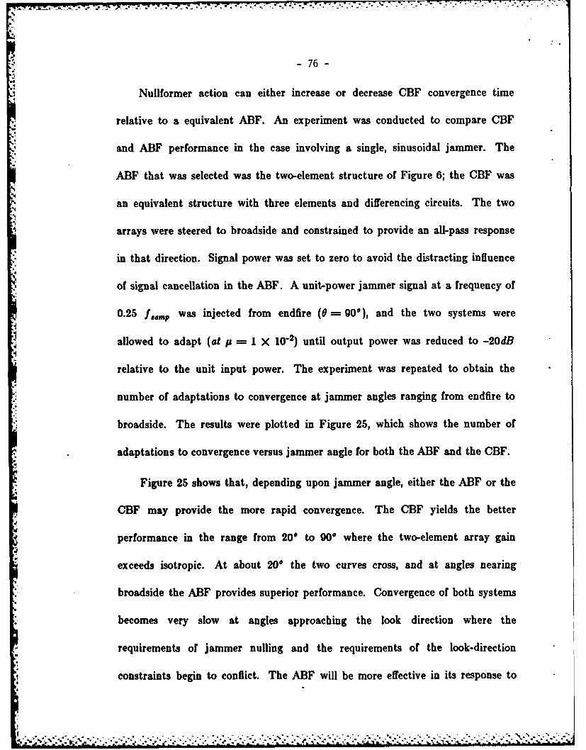
M --7 - 7W

-76-

Nullformer action can either increase or decrease CBF convergence time

relative to a equivalent ABF. An experiment was conducted to compare CBF

and ABF performance in the case involving a single, sinusoidal jammer. The

ABF that was selected was the two-element structure of Figure 6; the CBF was

an equivalent structure with three elements and differencing circuits. The two

arrays were steered to broadside and constrained to provide an all-pass response

in that direction. Signal power was set to zero to avoid the distracting influence

of signal cancellation in the ABF. A unit-power jammer signal at a frequency of

0.25 f,,rp was injected from endfire (0 = 0), and the two systems were

allowed to adapt (at p = 1 X 10-2) until output power was reduced to -20dB

relative to the unit input power. The experiment was repeated to obtain the

number of adaptations to convergence at jammer angles ranging from endfire to

broadside. The results were plotted in Figure 25, which shows the number of

adaptations to convergence versus jammer angle for both the ABF and the CBF.

Figure 25 shows that, depending upon jammer angle, either the ABF or the

CBF may provide the more rapid convergence. The CBF yields the better

performance in the range from 201 to 90* where the two-element array gain

exceeds isotropic. At about 20' the two curves cross, and at angles nearing

broadside the ABF provides superior performance. Convergence of both systems

becomes very slow at angles approaching the look direction where the

requirements of jammer nulling and the requirements of the look-direction

constraints begin to conflict. The ABF will be more effective in its response to

+ %"o2"'' " %P" " "°"" - "'+. " -'.-'•

+ . " :' : ... .. '" - ., ' . . ... ,C- +. -i , . '

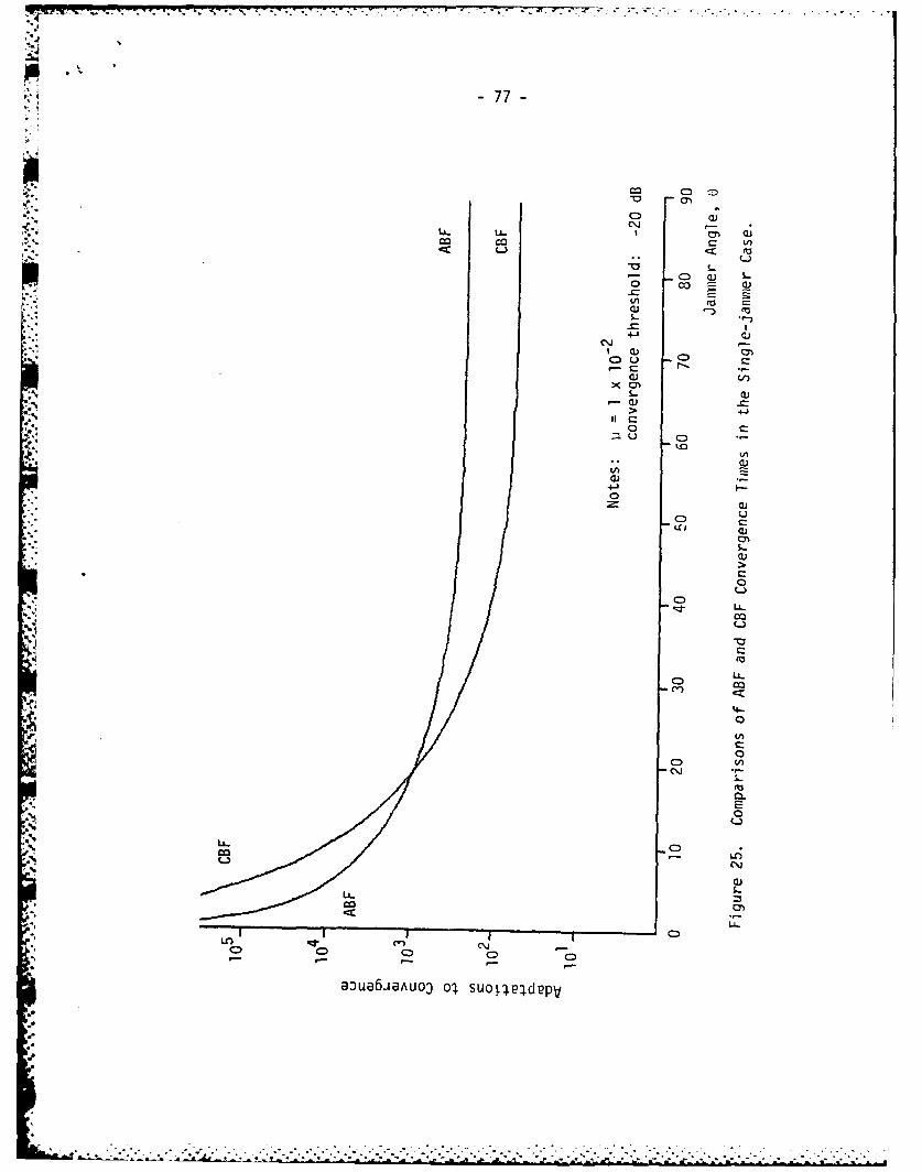
'.4 -77-

a M)

UI r-cn

S..

a) m

> 4-

L a)

'-a) a)

C)

a)a

4-' 4-

C) )

LL.

a)

~~LL.

C-)Ln c-)

C~'U

Cl CD C

aoua.AaUOD l SOLIPdP0

-78-

jammers arriving near the signal. On the other hand, the CBF will be somewhat

more tolerant of small errors in array steering because of its sluggish response at

angles near the look direction. It appears likely that, for small steering errors,

signal nulling in the CBF will be deferred indefinitely by a reasonably dynamic

electromagnetic environment or by the artificial injection of a small amount of

noise into the system.

D. Weight Quieting in the CBF

An important aspect of the performance of an adaptive system is its

behavior near the optimal solution. Ideally, the weights of an adaptive system

should move to the optimal solution, remain at precisely that point in weight

space, and displace only in response to a change in the optimal solution, i.e., in

*response to an actual change in the environment. In practice, a compromise

must be reached between the ability of an adaptive system to hold the optimal

*solution in a stationary environment and to track the optimal solution in a

nonstationary environment. The nature of the compromise is not necessarily the

same, however, from system to system. This section will compare the

performances of the Frost ABF and the Frost-based CBF near the optimal

solution and will show from another point of view that the CBF enjoys a

performance advantage.

Weight updating in the Frost ABF is accomplished in accordance with the

recursion relationships given in (2-14) or (2-17). The same weight updating

77 7I-- 7- 77-7 V'--- - -7--w- 71 rrC C--*.

-79-

technique is used in both the Frost ABF and the Frost-based CBF, but the data

samples entering the computations differ significantly as the two systems

approach convergence. The contrasts may be seen by examining any of the

weights; let the first weight w I be selected.

Initially the Frost ABF will be considered. The difference between the

values of w I at two successive samples may be written from (2-14) as

I K fiw l(k+ 1) - w 1(k) - -py(k)zl(k) - [w i(k) - py(k)z-(k)J + ,

j-+ K

(4-32)

. Because the constraint f is, by definition, the sum of the weights in the first

column of the beamformer, (4-32) may be simplified to

w 1(k+ 1) - w 1(k) = -py(k) [zl(k) - zj(k)]i=-i

(4-33)

Let it be assumed that at the kt sample instant the adaptive system has

reached a set of weights that closely approximates the optimal solution. Then

"""w l(k) w I (4-34)

Additionally, if the constraints are set to provide unity gain and an all-pass

response in the look direction, the system output is

y(k) s a(k) + nr(k) , (4-35)

where 8(k) is the signal at the kA sample time at any of the taps in the first

;" . "'-'.'...-.".-.. .-.- ..'.'..-°...''..,...-............ .- ,."- -' ."-" "2-2.' I -22-"-2-' i

-..L'!: " ' ' ' s - * . •

-80 -

column of the beamformer and nr(k) is the residual noise that exists at the

beamformer output with optimal weights.

The tap voltages in the first beamformer column may also be stated in terms

of signal and noise components:

- (k) - a(k) + ni(k) , i =1, 2, ..., K (4-36)

Note that the cophased signal is the same at taps I through K. This allows (4-

33) to be simplified to

[w.(k+ 1)- wl(k)ABF = -p[s(k) + n,(k)I [n, - - E nil (4-37)

The CBF weight recursion will now be considered under like circumstances.

" Again assume operation near W*. Further assume that the nulling-circuit

performance is nearly ideal so that differences in the noise voltages between the

CBF and a comparable ABF may be neglected. Then the CBF tap voltages are

; (k) = ni(k) , = 1, 2, ... , . (4-38)

The weight difference is obtained from (4-33) as

I K i 4-o[w l(k+ 1) -w l(k)]CBF = -p[ni(k)] [n, - -) nl (4-39)

The contrast between ABF and CBF weight behavior near convergence may

be seen by comparing (4-37) and (4-39); the difference lies in the inclusion of the

signal term in the ABF update expression.

--. 1

17i. .I. ;

.-- '-

The significance of this contrast is illustrated in Figure 26, which shows a

cut along the w I axis through the error surfaces of the two systems. Under the

assumption of negligibly different noise voltages in the ABF and CBF, the shapes

of the two error surfaces are identical. The ABF minimum, however, is

substantially elevated above the CBF minimum. If a useful signal is to be

delivered by the adaptive system, output signal-to-noise ratios in excess of 10 dB

are ordinarily required, and ratios in excess of 20 dB are certainly desirable.

These ratios imply that the signal levels will typically be three to ten times the

noise levels as the ABF nears convergence. The typical weight adjustment in the

ABF will thus be dominated by signal effects as the adaptive system nears

convergence. This becomes especially important when it is realized that the

signal-times-noise terms amount to short-term estimates of the correlation

between the signal and the noise. In other words, the signal influence in the ABF

should not be regarded as simply a random weight adjustment, but as a

I, purposeful step toward effecting signal cancellation. Because the CBF weight

adjustments are not influenced by the signal, the CBF weights exhibit less

variation about the optimal solution than the weights of the comparable ABF.

Further, the CBF weight adjustment process cannot cause signal cancellation.

-82-

~4-3

I-4--

I- 0

GJ

4-

0)di

m

" %-ilO;:X 6)

VP- -No I a C V I

-13-

V. SUMMARY AND CONCLUSIONS

It has been shown that interaction between the desired signal and

interference signals can lead to partial or total cancellation of the desired signal

within an adaptive beamformer (ABF). The signal cancellation phenomenon may

arise spontaneously in a multipath environment, or it may be deliberately or

accidentally induced by intentional or unintentional jamming. High adaptation

rates increase the susceptibility to signal cancellation in beamformers that have

not been designed to avoid the effect.

A composite beamformer (CBF) has been described that avoids signal

cancellation. The CBF makes use of both an adaptive beamformer and a

nonadaptive, slaved beamformer. The inputs to the adaptive beamformer are

preprocessed to exclude the desired signal, but retain representation of the.

interference signals. By restricting the adaptive process in this fashion, a solution

(i.e., a set of beamformer weights) is generated that influences only the

interference signals. Weights from the adaptive processor are copied to the

slaved processor, which is connected directly to the antenna elements and which

produces the useful output of the array. The CBF delivers much better

performance with regard to signal cancellation than a more conventional ABF.

Simulation data have been presented to show the improvement that can be

obtained.

The performance of a Frost-based CBF has been compared with that of a

* Frost ABF. If a narrowband system is assumed, it has been shown that the

-t....

- 84 -

Frost-based CBF will tend toward the optimal (i.e., the Wiener) solution

provided 1) the preprocessor admits energy from each jammer, 2) energy from

each jammer dominates the thermal noise, and 3) there are sufficient degrees of

freedom to null each jammer. The properly designed CBF is thus equivalent to

the comparable ABF in terms of the ideal solution. The CBF will not, however,

exhibit signal-induced weight variations. Performance will therefore be improved

in those cases where signal cancellation occurs in the ABF. Convergence toward

the optimal solution will, in general, be different for a CBF and an equivalent

ABF that are operating in the same environment. The convergence-rate

differences are governed by the influence of the preprocessor. In some cases the

CBF will attenuate a given interferor more rapidly than the ABF, while in other

cases the reverse is true. If the preprocessor is designed to match the basic array

element pattern except for a sharp null in the look direction, the convergence

rates for the CBF and the ABF are essentially the same. An exception occurs for

a jammer incident from very near the look direction. The CBF responds even

more sluggishly than the ABF to such an interferor. It is also true, however, that

the CBF is less sensitive to small steering errors than the ABF.

The studies of signal cancellation and the CBF have thus far suggested

several areas for further investigation. The signal cancellation phenomenon itself

is not so well characterized as might be desired. An improved characterization of

the phenomenon may provide a better means for analyzing the importance of

signal cancellation in various systems and environments. Additionally, this work

,- . '.,. - ,''.....:, . , s ,'. . -". , : . .. , -. .. :-.: '. - -.. ,:,",...-" , . .. -.

-85-

may reveal new ways to avoid the effect in adaptive arrays.

Perhaps the most promising area for further CBF improvement is in the

preprocessor that nulls the target signal. Work thus far has centered on the

element-differencing scheme because of its simplicity. Other preprocessor

configurations, though more complex from a hardware viewpoint, are capable of

yielding subarray patterns that provide a better match between the patterns seen

N by the adaptive beamformer and the slaved beamformer. Improved matching

will assure that the CBF performance (both dynamic and asymptotic) is

approximately that of the equivalent ABF, except for the superior CBF

performance with regard to signal cancellation. Steyskal [211 has recently

described a procedure for optimal pattern matching subject to null constraints.

This procedure appears to be well suited for preprocessor design.

The general procedure of adapting in the absence of signal can sometimes be

applied without resorting to the CBF. Systems that make use of low-duty-cycle

or frequency-hopped signals can employ other signal-exclusion schemes that arise

naturally out of the signaling format. Work is in progress at Stanford on

cancellation-free adaptation schemes for systems in these classes. These schemes

will trade timing constraints against the spatial-nulling method of the CBF and

will almost certainly result in less complex adaptation schemes for systems that

do not continuously occupy a channel.

-86-

REFERENCES

1. P. W. Howells, "Intermediate Frequency Side-lobe Canceller," U.S. Patent

3,202,990, 24 Aug. 1965 (filed 4 May 1959).

2. P. W. Howells, "Explorations in Fixed and Adaptive Resolution at GE and

SURC," IEEE Trans. Ant. and Prop., Vol. AP-24, pp. 575-584, Sept. 1976.

3. B. Widrow, P. E. Mantey, L. J. Griffiths, and B. B. Goode, "Adaptive

Antenna Systems," Proc. IEEE, Vol. 55, pp. 2143-2159, Dec. 1967.

4. L. J. Griffiths, "A Simple Adaptive Algorithm for Real-time Processing in

Antenna Arrays," Proc. IEEE, Vol. 57, pp. 1696-1704, Oct. 1969.

5. 0. L. Frost, M, "Adaptive Least Squares Optimization Subject to ,near

Equality Constraints," Ph.D. Dissertation, Stanford University, Stanford,

CA, Aug. 1970.

6. 0. L. Frost, M, "An Algorithm for Linearly Constrained Adaptive Array

Processing," Proc. IEEE, Vol. 60, pp. 926-935, Aug. 1972.

7. C. W. Jim, "A Comparison of Two LMS Constrained Optimal Array

Structures," Proc. IEEE, Vol. 65, pp. 1730-1731, Dec. 1977.

--- .'r_ t_ -* . .w ' , pF. r P7" ' m,, , " """*" " "(,, q 'p ' , ,,', "- .,"- .. ", *",*"-"" jN i . , ,€ ,, ,~ ,~n ,_ .n.h ,m ,, , ., a. .- - - - - - - .. .. .- '.% '''.,.. ..... ,... .',- ." '. .-- ° . ...." - '. -"-. .".

r t w- aS -.-

-87-

8. L. J. Griffiths and C. W. Jim, "An Alternative Approach to Linearly

Constrained Adaptive Beamforming," IEEE Trans. Ant. and Prop., Vol.

AP-30, pp. 27-34, Jan. 1982.

--.

9. R. A. Chestek, "The Addition of Soft Constraints to the LMS Algorithm,"

..a Ph.D. Dissertation, Stanford University, Stanford, CA, May 1979.

10. B. Widrow et al., "Adaptive Noise Cancelling: Principles and

Applications," Proc. IEEE, Vol. 63, pp. 1692-1716, Dec. 1975.

11. J. R. Glover, Jr., "Adaptive Noise Cancelling of Sinusoidal Interference,"

Ph.D. Dissertation, Stanford University, Stanford, CA, Dec. 1975.

12. J. R. Glover, Jr., "Adaptive Noise Cancelling Applied to Sinusoidal

Interferences," IEEE Trans. on Acoustics, Speech, and Signal Proc., Vol.

ASSP-25, pp. 484-491, Dec. 1977.

13. M. J. Shensa, "Performance of the Adaptive Noise Canceller with a Noisy

Reference - Non-Wiener Solutions," NOSC Tech. Report 381, Naval Ocean

Systems Center, San Diego, CA, 15 March 1979.

I14. M. J. Shensa, "Non-Wiener Solutions of the Adaptive Noise Canceller with

a Noisy Reference," IEEE Trans. on Acoustics, Speech, and Signal Proc.,

Vol. ASSP-28, Aug. 1980..4

. P , ' ,,, ' " ". ,".-,'',,"- ," ,"-. -'-" .'.- o''-.'-.''.-''- '. . .' ," .". -.".".".-L " - .a'.. .. '"..'.,' .' -"".' -' -" ,' -

:.,~~' - 88 -

15. B. Widrow, K. Duvall, R. Gooch, and W. Newman, "Jamming of Adaptive

Arrays by Signal Cancellation: the Phenomenon and Two Remedies,"

Proceedings of the 1980 Adaptive Antenna Symposium, RADC-TR-89-378,

Vol. 1, pp. 270-292, Dec. 1980.

. 16. B. Widrow, K. Duvall, R. Gooch, and W. Newman, "Signal Cancellation

Phenomena in Adaptive Antennas: Causes and Cures," IEEE Trans. on

Ant. and Prop., Vol. AP-30, pp. 469-478, May 1982.

17. R. T. Compton, Jr., Letter to B. Widrow referencing Figure 19 of

Reference 18, 23 May 1980.

18. T. Miller, R. Caldecott, and R. Huff, "A Satellite Simulator with a TDMA-

System- Compatible Adaptive Array," Report 3364-4, Electroscience

Laboratory, Ohio State University, Columbus, Ohio, Jan. 1976.

119. P. M. Hansen and J. P. Loughlin, "Adaptive Array for Elimination of

Multipath Interference at HF," IEEE Trans. on Ant. and Prop., Vol. AP-29,

-4 No. 6, Nov. 1981.

20. 1. J. Gupta and A. A. Ksienski, "Dependence of Adaptive Array

Performance on Conventional Array Design," IEEE Trans. on Ant. and

Prop., Vol. AP-30, No. 4, July 1082.

• .-..;.. ..-..v .° ." . - - . .. .. -. ... .. ... .-. .. . .""" ... , -. ,W..-"." " i'

" "" ' "...

" :"

'" " " , '"" '"' " ; : "

i 21. H. Steyskal, "Synthesis of Antenna Patterns with Prescribed Nulls," IEEE

:.', Trans. on Ant. and Prop., Vol. AP-30, No. 2, March 1g82.

-'

.4

9'0

APPENDIX A

ANALYSIS OF THE DYNAMIC SOLUTION

FOR THE SINUSOIDAL CASE

Chapter 2 discussed the dynamic solution that is tracked by an ABF when

large values of the adaptation parameter p; are used. A computer simulation

formed the basis of that discussion, and certain claims were made withouta

supporting analysis. In this appendix the dynamic error-surface minimum is

examined analytically, and a mathematical model is developed that supports the

discussion in Chapter 2.

In Chapter 2 the Frost ABF under study was mapped into an equivalent

adaptive noise canceller (ANC) in order to reduce the problem dimensionality and

simplify the analysis. This same mapping will be used here; Figure A-i reviews

the ANC structure that will be analyzed.

The ANC structure assumes separate availability of the desired signal and

the single jammer signal, both of which are sinusoids in the case under

consideration. The desired signal is taken directly to the output summing

junction 'M conformance with a unit-gain, all-pass constraint in the look

direction. The jammer signal is processed through a two-channel (in-phase and

quadrature) filter with one weight per channel and is subtracted from the desired

signal at the output summing junction. The ANC output is also the error signal

that is fed back to control adaptation of the filter weights. In the notation

HD-A133 676 RESEARCH ON ADAPTIVE ANTENNA TECHNIQUES V(U) STANFORD 2/2UNIV CR INFORMATION SYSTEMS LAB K M DUVALL ET AL.SEP 83 N@0019 82-C-0189

UNCLASSIFIED F/G 17/4 N

EEEEMMMEMMMMiEmEMhEEEEEEMhhEEMONEEONEEEEEI

liii111.0

IIIIL - 1111 1=4

MICROCOPY RESOLUTION TEST CHARTNATIONAL BUREU OF STANDARDS-1963-A

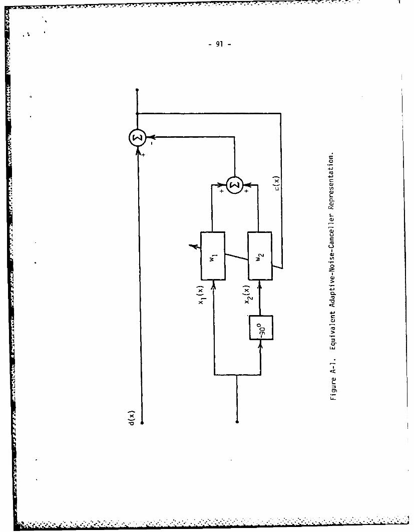
-91-

0

xw

U' (

* CA

0

I

CD eo

InJ

0U

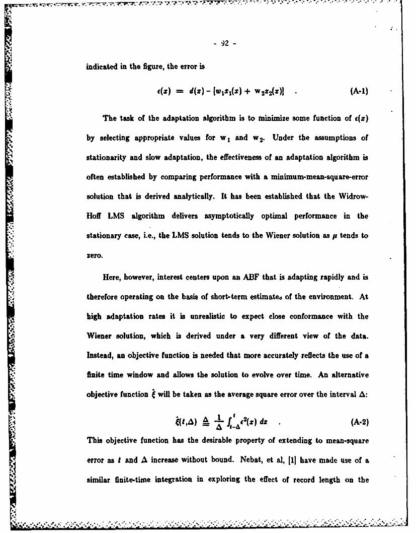
-92-

indicated in the figure, the error is

e(z) = d(z) - [wlxl(x) + w2X4(z)I (A-i)

The task of the adaptation algorithm is to minimize some function of f(Z)

by selecting appropriate values for w I and w2. Under the assumptions of

stationarity and slow adaptation, the effectiveness of an adaptation algorithm is

often established by comparing performance with a minimum-mean-square-error

solution that is derived analytically. It has been established that the Widrow-

Hoff LMS algorithm delivers asymptotically optimal performance in the

stationary case, i.e., the LMS solution tends to the Wiener solution as p tends to44

zero.

Here, however, interest centers upon an ABF that is adapting rapidly and is

therefore operating on the basis of short-term estimate* of the environment. At

high adaptation rates it is unrealistic to expect close conformance with the

Wiener solution, which is derived under a very different view of the data.

Instead, an objective function is needed that more accurately reflects the use of a

finite time window and allows the solution to evolve over time. An alternative

objective function C will be taken as the average square error over the interval A:

,) A -(Z) dZ (A-2)ea

This objective function has the desirable property of extending to mean-square

error as t and A increase without bound. Nebat, et al, (11 have made use of a

similar finite-time integration in exploring the effect of record length on the

a ' ** ** .d '

' " 4 4.... .4. - * . . . . . . . . . .... .

W7.- W- 77'

- 93 -

correlation of complex exponentials.

Combining (A-I) and (A-2) gives

2 2W2 tf~~tA)d 2(xdz - -- f d() 1 zdr ()2Z

2WW t 2.+ A _t:, (z)dz + 'a _ r,(z)(z)dr + A x2 (-)dz

(A-3)

To provide a more compact notation, let

r,y(t,A) A z ,(z)zi(z)dz i, j = 1, 2

p,(t,A) A I f d(z)zr(z)dz i = 1, 2 (A-4)

Equation (A-3) may now be rewritten as

t ) - -A d2(z)dz - 2w, pl(t,A) - 2w2 p2(t,A)

+ w? r,,(t,&) + 2wIw 2 r,(1,A) + w r2(t,A) (A-5)

Minimization of t(t,A) is accomplished by taking the gradient with respect

to the weights, setting the gradient to zero, and solving for w I and w 2. The first

two steps of this procedure yield

1-2 p1 (t,A) + 2w, rjj(t,A) + 2W2 r12(t,A) ".A

VCt,&) _ 12 P2(tA + 2w, rdf(SA) + 2W2 r22(*,A) J = o] (4

* The solution of (A-6) may be written as

* " " , . ." . . . . , . . . .. . . . o -

- 4 -

1 tmI = [r21(tA, ) r(t,4A) ] 1p2(t) (A-7)

where wim and w2 . are the values of the weights that minimize the objective

function during a given time window and where existence of the matrix inverse is

assumed. The equivalent matrix equation for (A-7) is

Wn = R-'(t,A) P(t,A) (A-8)

Equations (A-7) and (A-8) are finite-time-window versions of the familiar

Wiener-Hopf equation.

Since the dimension of (A-7) is only two, it is simple to expand the matrix

inverse and obtain expressions for the weights:

Win - 249,A) pllt,A) - r12(t,A) p2 t,A)

W2h. = (eR)I ) l(tA) p,(IA) + rII(t,A~) p2(t,(54 (A9)

Equations (A-9) describe the optimal weights for the two-weight adaptive noise

canceller at time t when averaging is over a window of duration A.

In order to obtain a direct comparison with the sinusoidal case considered in

Chapter 2, let

d(z) = cosw w

Z,(Z) = cos(W2 + )

z2(l) = sin (w2z+ ) (A-10)

/ ..- , ..' , ,. , .,'. ': '.,,. ..,. ' " . • . .. .. ..- . . . , . . . '. ,.. .. a . ,. ,. , , -. . - . . . .

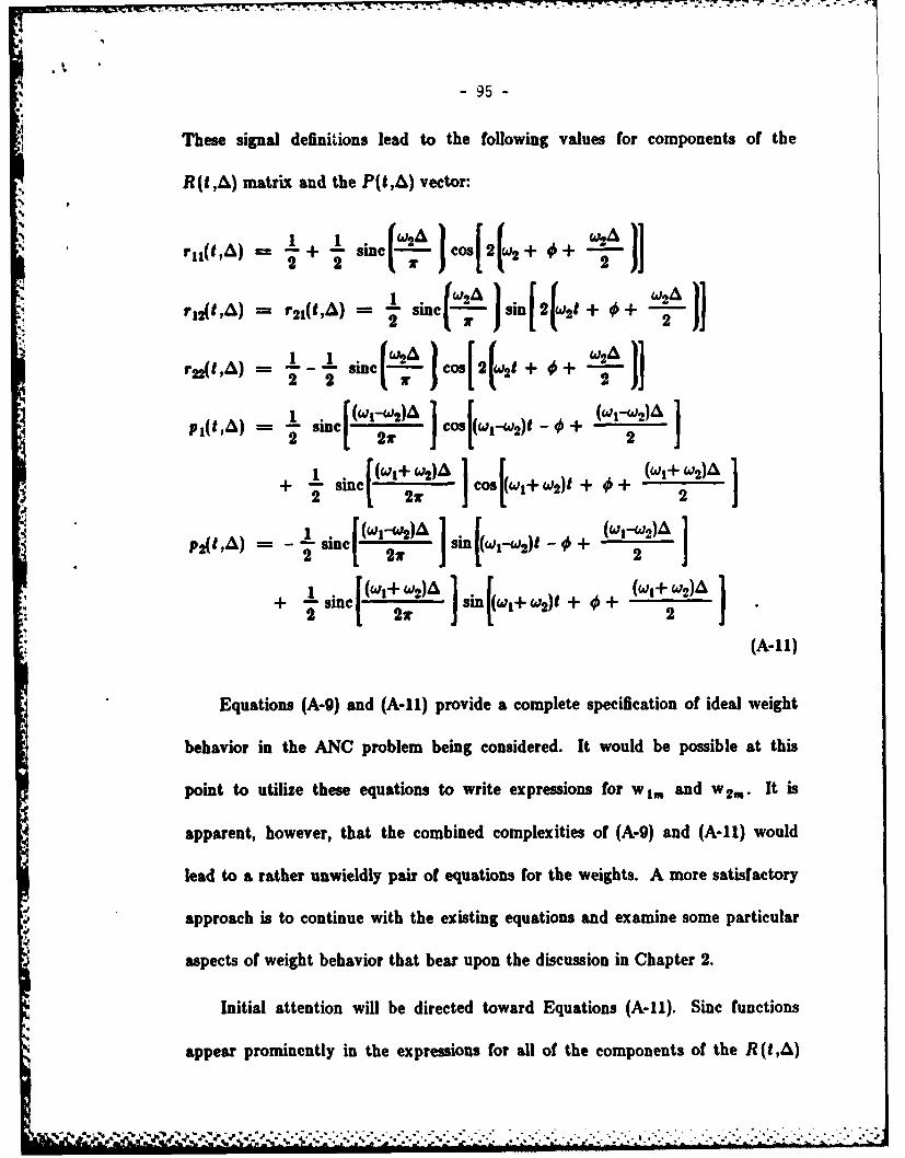
-95 -

These signal definitions lead to the following values for components of the

R(t,A) matrix and the P(t,A) vector:

r+ - sine +cos 2 + +

rz ?I(t,A) = I _ 1_. sin - o 2 LI + :2 2 r2

+ SI fl C l cos ,W2 )t + + d 2

PI(t,A) = - [-1sine Cos W" '--2)- + ( )

+ I sine((l+ W2)Isin ,W+ W)t + , + W 2)A

" (A-iI)

Equations (A-9) and (A-I1) provide a complete specification of ideal weight

behavior in the ANC problem being considered. It would be possible at this

point to utilize these equations to write expressions for wl, and w 2,. It is

'apparent, however, that the combined complexities of (A-9) and (A-i1) would

lead to a rather unwieldly pair of equations for the weights. A more satisfactory

approach is to continue with the existing equations and examine some particular

aspects of weight behavior that bear upon the discussion in Chapter 2.

Initial attention will be directed toward Equations (A-11). Sinc functions

appear prominently in the expressions for all of the components of the R (t,A)

I ~~~~~~......................................i.....l...mnmi~im ....

-96-

matrix and the P(t,A) vector. These sine functions govern the peak amplitudes

of most terms in the correlation expressions and thus play a key role in

determining weight behavior. The arguments of the sine functions involve only

the time window A and some function of w, and w2. This latter quantity is fixed

for a given problem statement, but the equivalent time window can be governed

in an adaptive system by choice of the adaptation parameter p. The observation

that weight amplitudes can be influenced by the choice of adaptation parameter

harmonizes well with the behavior observed in the experiments of Chapter 2.

A better understanding of the relative importance of the terms in (A-i1) can

be obtained from a closer study of the sine functions. Figure A-2 is a plot of sine

function magnitude as a function of the argument. An upper bound for the sine

function is also plotted to reflect the inverse dependency on argument that

dominates the sine function behavior. It is clear from the figure that a small

argument is necessary if the sine function is to contribute significant amplitude to

a term. Conversely, it is easy to see that, unless w, and w2 are equal, large values

of A will lead to large arguments and vanishing amplitude contributions from the

terms involving sine functions, i.e.,

lim rll(t,A) = 1A-.o0 2

lim r12(t,A) = lim r 1(t,A) 0At-00 A-00O

lim r(t,2A) = I.--,A -000 2

Z42

..I.--.-' '- " - ''' i - i .i - i • - , . . .. i " " . . -- ' ,.i" i -. '

- - .. S - - - .. - gZA % --.

-97-

3

Lfl

ca.CL

a)

3 J3.

4-

II C*j u

44-

0

4-0

UL-

p. 0 0 0 0o 0n 0I 0Y 0C

PUP C CO iP.U6 U

pu j oanj-

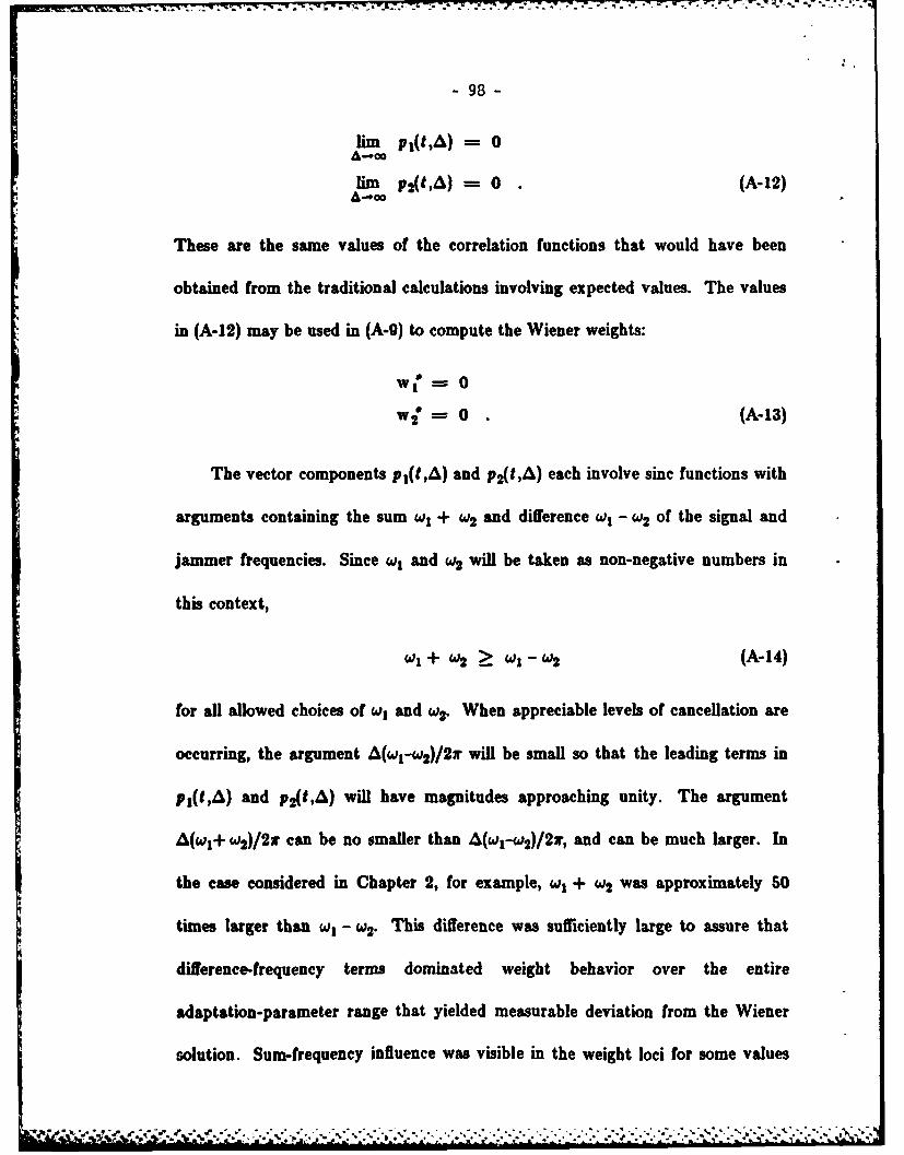
.... - 7 . .--.7. - . .-.

- 98 -

lim P 10 14) = 0A-oo

lim pt) = 0 .(A-12)

A-.*oo

These are the same values of the correlation functions that would have been

obtained from the traditional calculations involving expected values. The values

in (A-12) may be used in (A-9) to compute the Wiener weights:

wl - 0

w 2" = 0 (A-13)

The vector components pl(t,A) and p2(t,A) each involve sine functions with

arguments containing the sum w, + w2 and difference w, - w2 of the signal and

jammer frequencies. Since w, and u,2 will be taken as non-negative numbers in

this context,

WI + W2 2 WI - W2 (A-14)

for all allowed choices of w, and w2. When appreciable levels of cancellation are

occurring, the argument A(wI-w 2)/2" will be small so that the leading terms in

pl(t,A) and p2(t,A) will have magnitudes approaching unity. The argument

A(w + w2)/2r can be no smaller than A(wl-w2 )/2w, and can be much larger. In

the case considered in Chapter 2, for example, w, + w2 was approximately 50

times larger than WI - W2. This difference was sufficiently large to assure that

difference-frequency terms dominated weight behavior over the entire

adaptation-parameter range that yielded measurable deviation from the Wiener

solution. Sum-frequency influence was visible in the weight loci for some values

- 99 -

of the adaptation parameter, but never caused deviations of more than a few

percent from the basically circular loci.

It is useful to look more closely at weight behavior when difference-frequency

terms are dominant. Assume that w, and w2 are nearly equal and are sufficiently

different from zero so that

< 0.5 (A-5)

2v

and

W + W2 >> Col-jW 2 (A-16)

Under these circumstances, the difference-frequency terms in pj(t,A) and p2(t,A)

are dominant and

P1(tA - einc I w~ 2~1Cos Iw-W2) -+ (w ) +2 2w r 2 j

p2(,I ± [w1-'02)A wrw) (A-17)2 (L2i j 2 ]

Further, if sinc [ (Wl ) is negligible, then so is sine . This

observation allows the approximations

2

r1204,) =r 21(tA) = 0

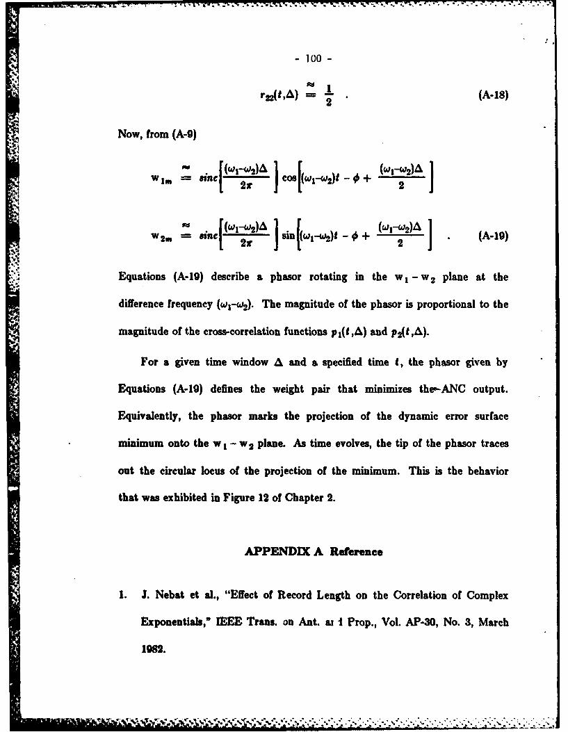
- 100 -

,.2(*,A) (A-18)

Now, from (A-g)

ON j '0'-w2)A ] Cos (WI-W2)t - +1W. sine[Lr 2 2 '

Wln sin (wl-.w2)t - + 2W2n se[ - W-) (I2) • A-)

Equations (A-lg) describe a phasor rotating in the w I -w 2 plane at the

difference frequency (w-w2). The magnitude of the phasor is proportional to the

magnitude of the cross-correlation functions pl(tA) and p2(t ).

For a given time window A and a specified time f, the phasor given by

Equations (A-19) defines the weight pair that minimizes theANC output.

Equivalently, the phasor marks the projection of the dynamic error surface

minimum onto the w I - w 2 plane. As time evolves, the tip of the phasor traces

out the circular locus of the projection of the minimum. This is the behavior

that was exhibited in Figure 12 of Chapter 2.

APPENDIX A Reference

1. J. Nebat et al., "Effect of Record Length on the Correlation of Complex

Exponentials," IEEE Trans. on Ant. at i Prop., Vol. AP-30, No. 3, March

1982.

L -

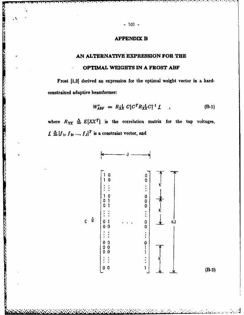
-101-

APPENDIX B

AN ALTERNATIVE EXPRESSION FOR THE

- OPTIMAL WEIGHTS IN A FROST ABF

Frost 11,21 derived an expression for the optimal weight vector in a hard-

constrained adaptive beamformer:

W6F = RjC[ C rR[ c - £. , (B-1)

where Ry 4L E[XXT ] is the correlation matrix for the tap voltages,

I AI 1, f , ..jl is a constraint vector, and

1I0 0- - - "10 0

1 00* . K

10 0

0 1 0• K

C 0 1 0 KJO0 0

0 0 000 00 l T

0 0 l . (B-2)

*, ; .-" *' - ,, ", ,....-.....,... ,,'".......".. ""-..".........-..-......."",.,..,..."...."-..-.-,,......."....--...-• " "..:J

102 -

is a constraint matrix. In this expression for WJt!F, the dependency on the signal

environment is given in terms of the tap voltages, i.e., in term of R.XX, which

may be estimated from X.

In this appendix it will be shown that an equivalent formulation for the

optimal weight vector may be given in terms of the vector N where

N = X- S (B-3)

is the vector of tap noise voltages that is obtained by deleting the desired-signal

component S. In particular, it will be shown that the equivalent expression is

W,1F = R -1CCTRjJkCJ- (B-4)

where RNN !! EINNTI is the correlation matrix for the tap noise voltages.

The balance of this appendix is broken into two sections. In the first section

the validity of (B-4) will be demonstrated for the narrowband case. The second

section will then examine the somewhat more complicated wideband case.

A. The Narrowband Case

In the narrowband case it is assumed that signal bandwidths are small

enough to allow incident signals to be characterized as sinusoids with amplitude

and phase variations that are slow with respect to the carrier frequency. Under

these circumstances a single complex weight is adequate to adjust the gain and

phase of each beamformer channel. That is, the tapped-delay-line filter

constituting each beamformer channel is replaced by an in-phase weight and a

i!... , ,, ; " i ' -."," '-: " - " ' ' " . ..""? '?" ' "" '"? -" ""'" -' ' '" "' - " ?""... - t ,-. ,,, ,,:., ,.,,..,,. ,"":" " """ -" ' . '--" " "' " -" ,-." - .-.,.,,. . -- .-. ." . . ..:''" " '

1U3 -

quadrature weight. For the narrowband Frost ABF, the constraint vector

becomes simply

L = , , (B-5)

with f I a complex number giving the in-phase constraint as its real part and the

quadrature constraint as its imaginary part. Additionally, the constraint matrix

takes a simple form:

C = [il "'' I 1 ._ • (- )

The correlation matrix Rx must be decomposed into its desired-signal

component and its noise component in order to proceed further. This may be

accomplished by rewriting (B-3) in the form

X = N+ S (B-7)

and then making use of the cophased nature of the signal to obtain

X = N + vs , (B-8)

where the signal amplitude is taken as /i. Now, (3-8) may be used to obtain

RXX = E[XXT ] = EINNT] + 1 JT

= RNN + eII1 , (13-9)

where Frost's assumption [1] of a lack of correlation between signal and noise

voltages has been used to simplify the expression for RXX.

It will be useful at this point to focus attention on the factor Rjj& C that

%". ..% '- .',; . . .". ,,. ". . . ., .- :".,--. - ,.' . .."- " '' .. .' . ". - " ",. . .. . • " . ' ." . . . ,,.. .. ,,,.,,. .. , .,. ." . . . *. .,' .,.. ,,*"- '-_ _ ' " '... ." " .•.. . .. .. ..."4 ' *. . . .',

- 104 -

appears twice in (B-1) and to make use of an observation by Baird and Zahm [3)

regarding the utility of the matrix inversion lemma in a closely related problem.

The lemma may be drawn from (4] in the following form:

If a nonsingular matrix H of order n can be written in the form

H = A + BDE , (B-10)

* where B, D, and E are n X p, p X p, and p X n, respectively, and A and

D are nonsingular, then

H- ' = A - ' - A-IB(D-I+ EA-'B) - E4 - . (B-I)

The lemma given in (B-il) may be used to invert RX- in

RAC - [RNN + 61 1 T-l1 I (B-12)

As a preliminary step it is noted that RNN, which is analogous to the A matrix

in (B-10), is invertible because it is assumed to be positive definite. The vectors

s1 and 1 T, which correspond to B and E in (10), are K x 1 and 1 x K,

respectively. The D matrix in (B-10) degenerates to the scalar I in (B-12) and is

clearly invertible. With the applicability of the inversion lemma established, (B-

12) may be written as

s R IV ITR R 1RjjC = [Ri - 1+* IT RFVNIl)

Expanding gives

I 4 -.

- - - - - -

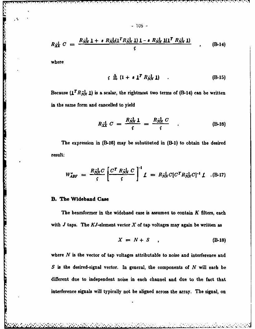
105-

Rja C NNRjJ 1 + 8 Rik(j R i k 1)1 -8 Rik 1 (j Rik 1) (B-14)

where

4(I + S i r Rik 1)

Because (lTR-N 1) is a scalar, the rightmost two terms of (B-14) can be written

in the same form and cancelled to yield

RAC - N (B-is)

The expression in (B-16) may be substituted in (B-i) to obtain the desired

result:

-- RNC[CTRN CI ,£ .(B-17)W18F -- -C NNf , , -

B. The Wideband Case

The beamformer in the wideband case is assumea to contain K filters, each

with J taps. The KJ-element vector X of tap voltages may again be written as

X = N+S

where N is the vector of tap voltages attributable to noise and interference and

S is the desired-signal vector. In general, the components of N will each be

different due to independent noise in each channel and due to the fact that

interference signals will typically not be aligned across the array. The signal, on

-" .

-106-

the other hand, is aligned across the array and is therefore identical down any

column of taps within the beamformer. The special structure of S may be

expressed by the relationship

S =CR , (B-19)

where C is defined by (B-2) and

R i. [s(k) s(k-r) a(k-2r) ... s(k - (J-l),) jr (B-20)

is the vector of desired-signal voltages at the taps of any beamformer delay line.

Combining (B,-18) and (B-19) yields

X = N+ CR (B1-21)

The correlation matrix for the wide band case may be computed based upon

(B-21):

RX = E[(N + CR)(N r + RTCT)j (B-22)

RXy = E[NNT ] + CEIRR T] CT (-23)

The transition from (B-22) to (B-23) has made use of the assumed lack of

correlation between signal and noise. Alternative forms for (&-23) are

RXX RNN + C RRR CT (3-24)

and

RXX RNN + RSS (3-25)

It should be noted that RNN and Rss are dimensioned KJ x KJ, while RRR is

,. S.. * ,,. ........ ...... "... ... ,.-... ... .... "-..... .... ... ,"....

-107-

dimensioned J x J. The difference in dimension between Rss and RRR reflects,

of course, the redundancy in RSS.

The matrix inversion lemma that was used in the narrowband case will

again be used to invert the matrix Ryx as expressed in (B-24):o'

.*i. RA- = RI,-V ICRI, + CT RI.C-' CTR-1 . (B-26)

Both RNN and RRR are assumed to be positive definite and therefore invertible.

The relationship given in (B26) will now be used to structure components of

the expression for WJF given in (B-I). The leading factor is easily constructed

• -. by postmultiplying (B-26) by C:

R C = RjJC - RNjkC[RJt + CTRj CI-I CTRfC " (B-27)

The central factor is obtained in two steps. First, (B-27) is premultiplied by

CT:

CTRj&C = [CTRI C1 + [-CTRRCj [RjJz + CTRjVC]-l [CTRj C]

(B-28)

The matrix inversion lemma is then applied once again to obtain:

[CTRiIC] -I [CTR C]- + [CTRvC] -I [CTRRNICI ( [R -1 + CTRR4CI

- [ -1RCIICTRRNC-I [CTRiVkCJ}-

lC'r R j&CJfCTRR IC, - I

[CTRcCI-I - [CTRiJNCI- + RRR (B-20)

Equations (B-27) and (B-29) may now be used to synthesize

N . . . . . .... ... ... . .... - . - ..at .. a. ' '.p.- ;....;.-;.... % .- . *--- - -- . a'2 .-% . . -i.i -'' - .' ' -, . " . ' " . -

* .**... - " " .

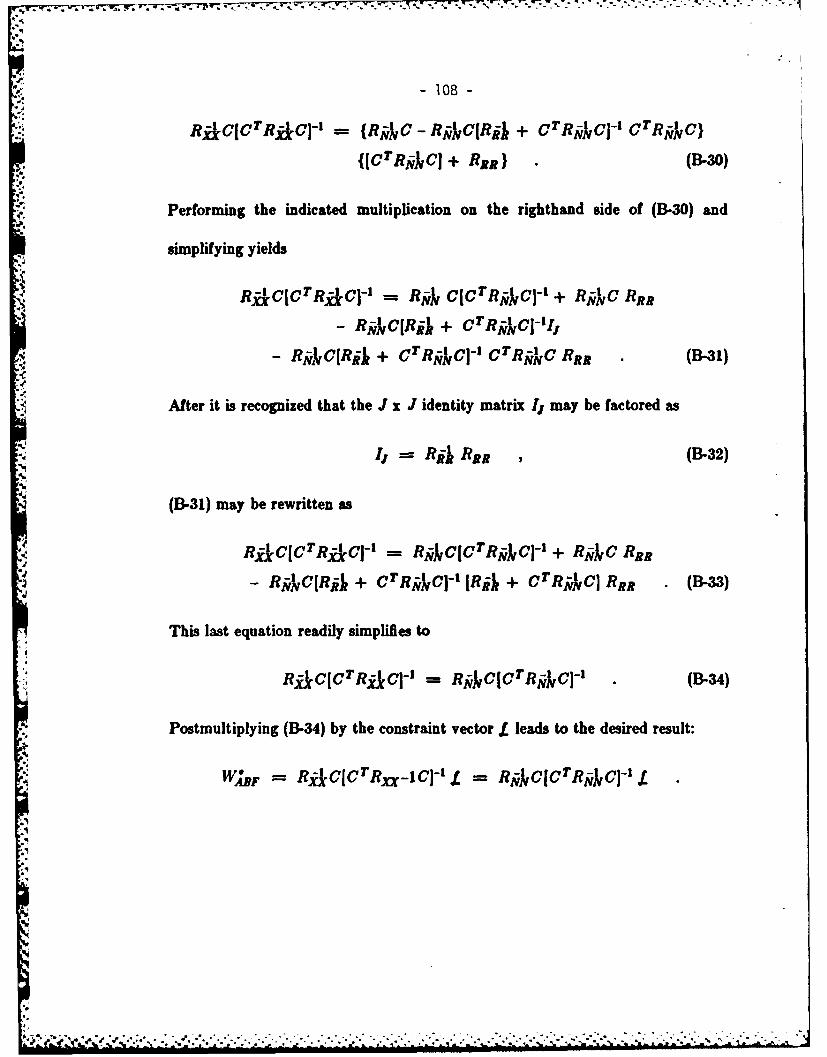
- 108 -

RIicICTRjJCl-l = R C - RJCjRjj + CTR Ci-' CrRjC)

{UcTRAcI + R ,) . (B-30)

Performing the indicated multiplication on the righthand side of (B-30) and

simplifying yields

Rj&CICTRj&cI -I = Ril C[CrRjjCJ- ' + RjC RRR- R1NC(Rij + cTRijkCI-II,

- Rj-VC[Rj + CTRgCJ-' CTRIC RRR • (B-31)

After it is recognized that the J x J identity matrix I, may be factored as

.;* = Rjjj Rqt (B-32)

(B-31) may be rewritten as

R,&C[CrjCJCl- = R 2JCjCT RjC - ' + RRNJ C RRR

- RjNCIRIL + cTRj-kC-l- IJR + CrRjkc ] RR, (B-33)

This last equation readily simplifies to

-RijCIcTR i -CCII- RjkCjCTR-1 -CI-I (B-34)

Postmultiplying (B-34) by the constraint vector . leads to the desired result:

= 6 RjjCCrR,_-1CJ1 f RgNCCTR - CII

1. '."e - • "d "t'. -'et " - - . - " "". . . . . . .""" " " " "' . .. ".. .. " . .. .

.A-. - 109 -

APPENDIX B References

1. 0.L. Frost M, "An Algorithm for Linearly Constrained Adaptive Array

Processing," Proc. IEEE, Vol. 60, No. 8, Aug. 1972.

2. 0. L. Frost III, Adaptive Least Squares Optimization Subject to Linear

Equality Constraints, Stanford Electronics Lab, Stanford, CA, Doe. SEL-70-

055, Technical Report 6796-2, Aug. 1970.

3. C. A. Baird, Jr., and C. L. Zahm, "Performance Criteria for Narrowband

Array Processing," Proc. 1971 IEEE Conference on Decision and Control,

Miami Beach, FL, 15-17, Dec. 1971.

4. B. Noble, Applied Linear Algebra, Prentice-Hall, Englewood Cliffs, N. J.,

' 1969.

.1. i k k .. .. d J . s w .. .saf- '. .a..' . -

-110-

APPENDIX C

AN ANALYSIS OF SIGNAL INFLUENCE BASED

UPON THE GENERALIZED SIDELOBE CANCELLER

4o

Another vehicle for analyzing the role of the desired or look-direction signal

is provided by the Grifliths-Jim generalized sidelobe canceller [1,2], a form of

which is diagrammed in Figure C-I. In this beamformer there is a fixed processor

(shown at the right side of the figure) that operates directly upon the signals

from the array and implements the look-direction constraints as stated by

(fi, i =1, 2, ..., N. Note that the look direction is perpendicular to the array

in the case shown; steering delays are needed for other look-direction choices.

There is also a second, adaptive processor that operates upon the difference

signals between adjacent elements and therefore is not exposed to look direction

C. signals through the eignal vector .* The output of the adaptive processor is

subtracted from the output of the fixed processor to obtain a useful signal. This

signal also constitutes the error signal that is used in an LMS update algorithm

as opposed the more complicated constrained LMS algorithm that would

otherwise be needed to implement hard constraints. It has been shown [2], that

9.; the Frost ABF and the generalized sidelobe canceller generate equivalent

solutions when the sidelobe canceller takes the particular form shown inT htere is, however, xpouue t the look-diction dpia throgh the errr ulpal that is ed back to direct adap-

Wes; the esetaised sildeobe eaaeeler is nbject to siplal caseeldloa.

C CL

:4-J

0j

dt

V4-

-j 0j

a, 0

+V

212

494 0

-R 0

- 112 -

Figure C-1.

In terms of the difference signal vector X1 and the signal d, the Wiener

weight vector for the generalized sidelobe canceller may be written as

W c= Rj~~ (C.d)

where

X, Z.; , ...ZjNNIT

RrrX 4E IX, X, T

PX' d E[dX'I . (C-2)

A representative element zi, 1 < i < K-1, of the difference signal vector

X' is obtained from the received signals according to

4Z = Zi - Zi_ . (C-3)

(The remaining elements of X1 were derived in the same manner at an earlier

point in time.) Each received signal is taken to consist of a signal component plus

noise components. Because the array is assumed to consist of identical elements

and to be perfectly steered, the signal components are identical across the array.

Therefore

*Zi - (=+nji-(+n -1 ) =-- n8-n+_1 (C-4)

It is evident from the lack of signal components in the difference signal vector

that the factor RjIX , can bring no signal influence to the Wiener solution.

The output d of the fixed beamformer in the generalized sidelobe canceller is

S. . . .- ., . . .,.

-13-

given by

K K Kd K E( e+ ni) =8s+ E~ n (C-5)

i°K im

The crosscorrelation may be calculated from X8 and d as follows:

Px . E~dX'!

= Effe + ± n)X'Jsi

- EIK' + E(l n[X'L4.' A i-.!

K

= Ellj N ,)X'] (0-6)s--I

It is now seen that the second factor of Equation (C-i) is also free of signal

influence and therefore that the Wiener solution for a hard-constrained ABF is

uninfluenced by the desired signal.

APPENDIX C References9

1. C. W. Jim, "A Comparison of Two LMS Constrained Optimal Array

Structures," Proc. IEEE, Vol. 65, pp. 1730-1731, Dec. 1977.

2. L. J. Griffiths and C. W. Jim, "An Alternative Approach to Linearly

Constrained Adaptive Beamforming," IEEE Trans. Ant. and Prop., Vol.

AP-30, pp. 27-34, Jan. 1g82.

'

-114-

APPENDIX D

A COMPOSITE BEAMFORMER BASED UPON

WIDROW'S PILOT-SIGNAL ALGORITHM

The composite-beamformer discussions in the body of this report centered

upon the use of Frcst's algorithm for weight adaptation. Frost's algorithm is

designed to operate in a signal-aligned environment, i.e., the array must be

steered either mechanically or electrically so that signals from the look direction

are cophased across the array. Once the array has been properly steered, the

Frost algorithm provides excellent control over the response in the chosen look

direction. The Frost-based CBF is an appropriate choice when a single look

direction can be established with reasonable accuracy.

In many cases, however, it is not possible or desirable to specify a single

direction of arrival for desired signals. These situations arise, for example, when

communications must be maintained with multiple stations, when the location of

a station is imprecisely known, or when motion of the receiving platform makes it

difficult to maintain high pointing accuracies. An alternative to the single, hard-

constrained look direction is needed in these cases.

There are two requirements that must be met in order to realize a CBF that

provides multiple look directions. The first requirement is to eliminate signal

energy incident from the various look directions. It is difficult and expensive to

generate wideband nulls in multiple directions. On the other hand, it is relatively

... .. ... .. ... .. ... .. ... .... -... ... .. .. . .-.

115-

simple to create multiple narrowband nulls by using a structure such as a nulling

.~ tree. The second requirement is to adaptively eliminate jammer signals while

sustaining useful responses in the look directions. Widrow's pilot-signal

algorithm provides a convenient method for nulling jammers while maintaining

soft-constrained responses in multiple look directions. Taken together, the

nulling-tree preprocessor and the pilot-signal algorithm form the building blocks

for a CBF that can serve multiple, narrowband signals.

The balance of this appendix describes the pilot-signal CBF and draws some

* comparisons with the basic pilot-signal beamformer. The first section discusses

the nulling-tree preprocessor and illustrates the use of the nulling tree to generate

multiple notches and broadened notches. The next section then explains the

CBF structure, which essentially consists of a nulling-tree preprocessor plus a

pilot-signal beamformer. The final section shows that, in contrast with the basic

pilot-signal ABF, the pilot-signal CBF is capable of generating an unbiased

solution for the narrowband case.

'4t A. The Nuliing Tree

The nulling tree was described by Davies [1) and is also termed the Davies

cascade or Davies null-steering network. As has been noted by Steinberg [21, the

nulling tree does not necessarily constitute the most efficient means of realizing

multiple nulls. The great virtue of the nulling tree lies in its ability to provide

independent control over multiple nulls. In that sense the nulling tree is well

.

S- 116 -

matched to Widrow's pilot-signal algorithm, which provides independent control

through the separate pilot signal established for each look direction.

The structure of the nulling tree is shown in Figure D-1. The tree consists

of a number of stages equal to the number of nulls to be generated. Each stage is

formed from a set of identical sections. The sections operate upon two outputs

from the preceding stage and perform a phase-shift-and-add process that nulls

signals arriving from a selected direction. In particular, a null is generated in the

0tA stage for signals arriving from an angle 0 by choosing the phase shift 4 given

by

-2?r d sin 0Xd + jr radians , (D-1)

where d is the interelement distance in the uniform linear array and X is the

wavelength at the frequency for which nulling is desired.

A computer program was written to design nulling trees and plot the

beampatterns resulting from the designs. Various test cases were examined to

determine the characteristics of the nulling-tree preprocessor.

Figure D-2 shows a series of beampattern pilots that result from adding

successive nulls at separate arrival angles. The initial null is established for

signals arriving from broadside; the second stage nulls signals from + 45'; and

the third stage is set for -30' arrivals. This preprocessor can accommodate an

environment in which there are multiple signals sources at well-defined look

directions.

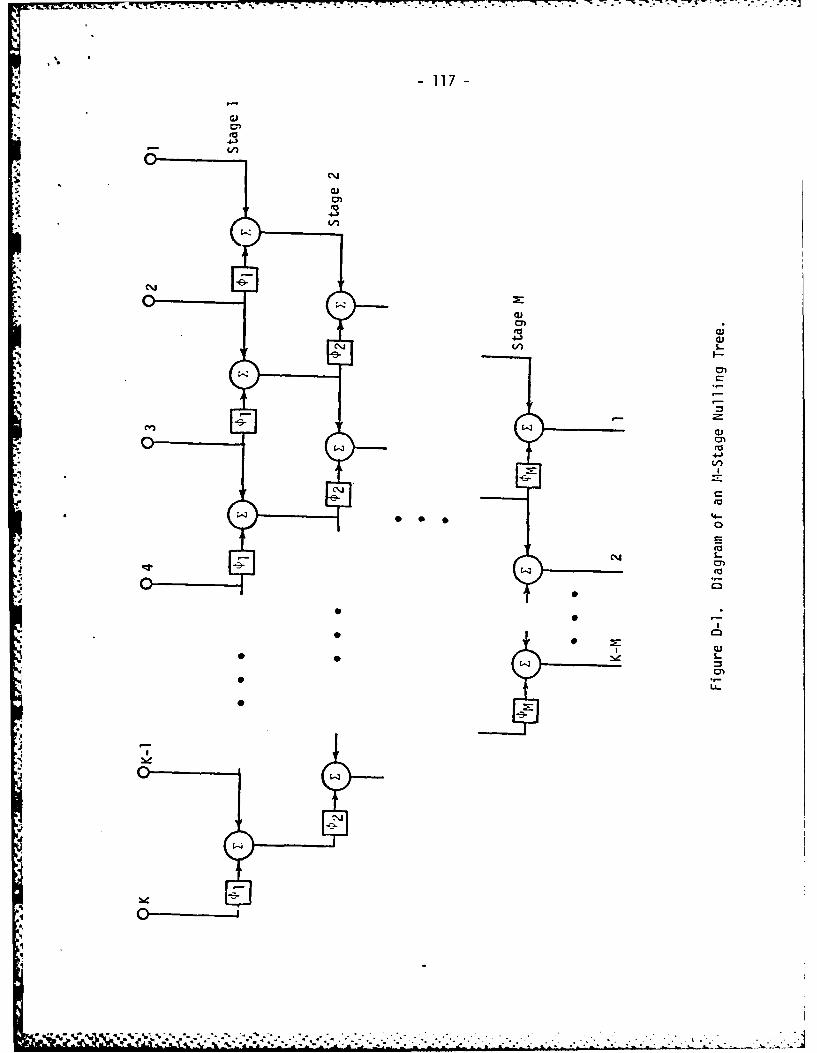
-117-

cmi

C-I-

0-0

GiE4 . L

*" L.

I-90i

*~*%*%**~ ~ .~. ... %.~...-. *.*4--

S-.

O

CD LO

Ln

0

4-)

- 0

/ CL

040

LOL

'~ L .0 r- co

qp 'asuodsab ADMOd PaZ L WON

pee.

____ f 'U--. U - . . . -

-119-

Another type of requirement is considered in Figure D-3. Here it is assumed

that only one emitter is of interest, but the look direction is imprecisely known.

An initial null is established in the estimated look direction, and successive stages

are used to broaden the null by creating additional spatial notches on each side

of the estimated direction.

B. Structure of the Pilot-Signal CBF

Figure D-4 is a block diagram of the pilot-signal CBF. A uniform linear

array of K elements provides the input signals to the CBF. All of the elements

are connected to the nulling-tree preprocessor, which consists of M stages that

create M nulls in the various directions from which desired signals may arrive.

The K-M outputs from the nulling tree constitute a signal-free environment in

*i which adaptation can proceed without concern about cancellation effects. The

slaved beamformer is connected directly to the first K-M elements of the array

and is used to derive a useful output signal for the receivers.

The pilot-signal algorithm is used to provide a prespecified, soft-constrained

response in each potential look direction. A separate pilot signal is generated for

each look direction and, after appropriate phasing, is added to the ABF inputs.

The pilots are also filtered and summed to form a synthetic "desired" signal

against which the ABF output is compared. The difference between the summed

pilots and the ABF output is the error signal that is used to guide adaptation.

• . . . . .. . . . . . .. ,- . . ,, . ..,. , . . .. ,... . . . . ,.... . .. .. ..

120-

CD a

CD 4.)4 co

CD 0

C4.

0 'U

C-

't

41)

0-

41

r S.

0)

I (V

conLA.

I I ICD

gpj 'audaj. LndPZ.1u.0

4plsos jmdPZ~uO

-121 -

4J

CLS _ _ _ __ _ _ _ _ _

C)

> 0

a) co

4-'0

c 0.

00

ea EL

coUCLC

00

CL 0

S. Li..

122-

Weight adaptation can be accomplished with a variety of different

algorithms. The Widrow-Hoff LMS algorithm 131 was initially proposed for use in

a digital implementation of the pilot-signal ABF. Applebaum 141 described an

analog implementation that makes use of correlation loops.

It is interesting to note that very few changes are needed to transform the

basic pilot-signal ABF into a pilot-signal CBF. The slaved beamformer is already

present in the pilot-signal scheme and therefore need not be introduced. The

only new components are the null-forming preprocessor and the extra antenna

elements entailed by the nulling process.

C. Bias Removal by the CBF

Soon after the development of the pilot-signal algorithm, it was recognized

that the solution it generates in the presence of signal is biased from the Wiener

solution. Griffiths [5] investigated the source of bias in some detail and succeeded

* both in explaining the phenomenon and devising an alternative beamformer that

avoided the problem. Griffiths' beamformer, however, is subject to signal

cancellation. The paragraphs that follow will demonstrate that, in addition to

solving the signal-cancellation problem, the CBF solves the bias problem, thus

eliminating both disadvantages normally encountered with pilot-signal

beamformers.

-123-

Griffiths investigated the bias issue in the context of a pilot-signal ABF with

a single look direction and, consequently, a single pilot signal. The same

approach will be followed here because the use of multiple pilot signals

complicates matters without contributing anything of substance.

The pilot signal in Griffiths' model is taken to be some multiple # of the

estimated desired signal i(k), i.e.,

d(k) = #i(k) • (D-2)

After phase shifting to allow for propagation effects, the pilot is added to the

beamformer inputs. This injected signal vector is identified as #,(k), where S(k)

is the estimated desired-signal vector across the inputs.

Weight updating is accomplished using the LMS algorithm:

- W(k+ 1) = W(k) + 2p( (k) - IXT(k) + PST(k)] W(k)) {X(k) + fS(k)}

(D-3)

where

X(k) is the input signal vector,

W(k) is the beamformer weight vector, and

p is the adaptation parameter.

Griffiths showed that the limiting value of the expectation of the weight

vector is given by

i)!

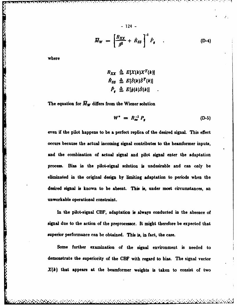
• + , ° -. . -- + . - + -.. . . + - . • _ . .. 7 .. . .. . . .

- 124 -

Vw = + Itss Pt (D-4)

where

Rx r EIX(k)XT(k)]

ASS E[D(k)§(k)J

The equation for Mw differs from the Wiener solution

w" = R, (D-5)

even if the pilot happens to be a perfect replica of the desired signal. This effect

occurs because the actual incoming signal contributes to the beamformer inputs,

and the combination of actual signal and pilot signal enter the adaptation

process. Bias in the pilot-signal solution is undesirable and can only be

eliminated in the original design by limiting adaptation to periods when the

desired signal is known to be absent. This is, under most circumstances, an

unworkable operational constraint.

In the pilot-signal CBF, adaptation is always conducted in the absence of

signal due to the action of the preprocessor. It might therefore be expected that

superior performance can be obtained. This is, in fact, the case.

Some further examination of the signal environment is needed to

demonstrate the superiority of the CBF with regard to bias. The signal vector

X(k) that appears at the beamformer weights is taken to consist of two

•-.

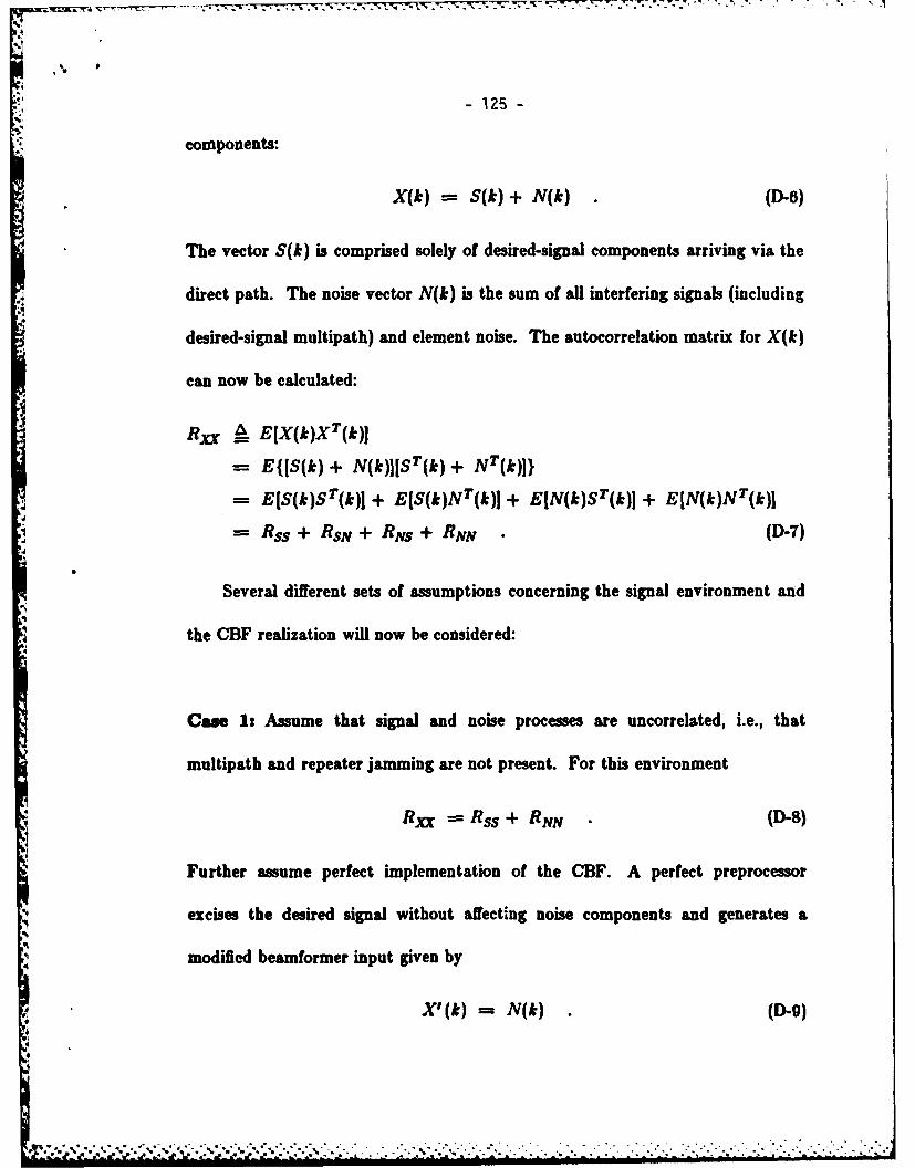
-125-

components:

X(k)--- S(k) + N(k) . (D-o)

The vector S(k) is comprised solely of desired-signal components arriving via the

direct path. The noise vector N(k) is the sum of all interfering signals (including

desired-signal multipath) and element noise. The autocorrelation matrix for X(k)

can now be calculated:I

R, 3 9_ E[X(k)X T (k)]

= E{IS(k) + N(k)IS T(k) + NT (k)])

E(S(k)ST(k)] + E[S(k)N T (k)] + E[N(k)S T (k)] + EIN(k)N T(k)]

RSS + RSN + RNS + RN (D-7)

Several different sets of assumptions concerning the signal environment and

the CBF realization will now be considered:

Case 1: Assume that signal and noise processes are uncorrelated, i.e., that

multipath and repeater jamming are not present. For this environment

RXX =Rss + RNN . (D-8)

Further assume perfect implementation of the CBF. A perfect preprocessor

excises the desired signal without affecting noise components and generates a

modified beamformer input given by

X,(k) N(k) . (D-9)

r . " ... •,, : , .... "...-].... .... i ~ l il'~i ii~ ii.-. W wiis

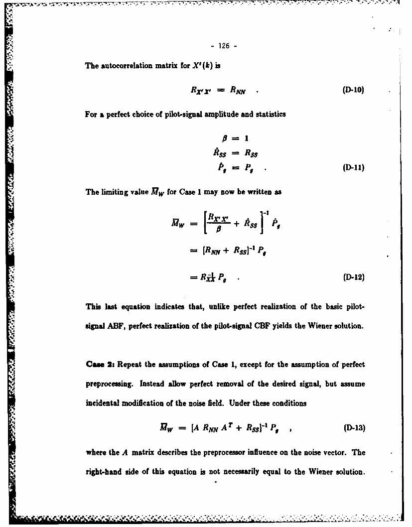
-126-

The autocorrelation matrix for X' (k) is

*. Xrr = RNN .(D-10)

For a perfect choice of pilot-signal amplitude and statistics

Rss = RSSR=P

r f I(.)

The limiting value MW for Case I may now be written as

]-I

= [RN + RssI-' Pg

= RA P, . (D-12)

This last equation indicates that, unlike perfect realization of the basic pilot-

signal ABF, perfect realization of the pilot-signal CBF yields the Wiener solution.

Can 2: Repeat the assumptions of Case 1, except for the assumption of perfect

preprocessing. Instead allow perfect removal of the desired signal, but assume

incidental modification of the noise field. Under these conditions.4

1w = [A RNN AT + RssI- PV , (D-13)

where the A matrix describes the preprocessor influence on the noise vector. The

right-hand side of this equation is not necessarily equal to the Wiener solution.

j "- . * * ' * . - . .. * .-, . -- - . u .. .. ...... . . . . . . . . . . .

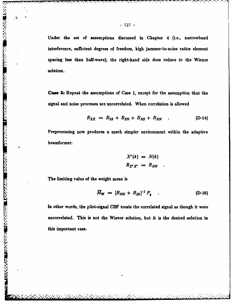
4 -IFT 1-

127-

Under the set of assumptions discussed in Chapter 4 (i.e., narrowband

interference, sufficient degrees of freedom, high jammer-to-noise ratios element

spacing less than half-wave), the right-hand side does reduce to the Wiener

solution.

Cam 3: Repeat the assumptions of Case 1, except for the assumption that the

signal and noise processes are uncorrelated. When correlation is allowed

Rxx = Rss + RSN + RNS + RNN - (D-14)

Preprocessing now produces a much simpler environment within the adaptive

beamformer:

X '(k) = N(k)

Rr X, = RNN

The limiting value of the weight mean is

iw = [RNN + Rss[' P, (D-1)

In other words, the pilot-signal CBF treats the correlated signal as though it were

uncorrelated. This is not the Wiener solution, but it is the desired solution in

this important case.

.-. *' "*/ I... *.. .. .... r . -. .... '.". . ......... .................. ... . 4

- 128-

APPENDIX D References

1. D. V. N. Davies, "Independent Angular Steering of Each Zero of the

Directional Pattern for a Linear Array," IEEE Trans. Ant. and Prop., AP-

4.~ 15, pp. 296-298, March 1967.

2. B. Steinberg, Principles of Aperture and Array System Design, John Wiley

and Sons, New York, 1976.

3. B. Widrow, P. E. Mantey, L. J. Griffiths, and B. B. Goode, "Adaptive

'. Antenna Systems," Proc. IEEE, Vol. 55, pp. 2143-2159, Dec. 1967.

4. S. P. Applebaum and D. J. Chapman, "Adaptive Arrays with Main Beam

Constraints," IEEE Trans. Ant. and Prop., Vol. AP-24, pp. 650-662, Sept.

1976.

5. L. J. Griffiths, "Signal Extraction Using Real-time Adaptation of a Linear

Multichannel Filter," Ph.D. Dissertation, Stanford University, Stanford, CA,

Jan. 1968.

I ..... ....44;

-129

APPENDIX E

SIMULATION METHODS

Computer simulations of the Frost ABF and the Frost-based CBF were used

to illustrate signal-cancellation effects and to demonstrate the performance

contrasts between the two beamformers. This appendix outlines the simulation

methods that were employed.

A. Simulation Facility

* The adaptive-antenna simulations for this research were performed on an HP

1000F minicomputer facility at Stanford University. The simulation software

was, for the most part, an existing Fortran package that was written by a team

of students* during 1079-1980 under the joint sponsorship of the U. S. Air

Force's Rome Air Development Center and the Naval Air Development Center.

The software package is organized as a set of programs that run under the

control of a driver program and exchange data through disk files. This

arrangement allows multiple simulation functions to be performed in parallel

(albeit on a time-shared basis) and facilitates research by allowing time-

consuming adaptation experiments to proceed in the background while

experiment preparation and data analysis are being performed by the user. The

software package is capable of simulating several different beamformer types and

Priatipd co-tributon were R. Gooch, W. Knalag, T. McCany, W. New-an, ud P. Titchemer.

n'..'i u nm -m i ii*i i 9.%:---

-130-

is sufficiently flexible to support most of the basic investigations that might be

* required for a specified adaptive antenna and signal/jammer scenario.

B. Simulation of an Adaptive Antenna

The program flow for adaptive antenna simulation is shown in Figure E-1.

The initial step in preparing a simulation experiment is to thoroughly specify the

"* problem that is to be considered. The driver program organizes this process by

prompting for the inputs that are needed to specify the following:

A. Antenna configuration

1. Number of elements

2. Location of each element

B. Beamformer structure

1. Number of taps per beamformer filter

2. Adaptive algorithm

3. Constraints (if applicable)

4. Initial weight values

C. Signal/jammer scenario

1. Number of signals/jammers

' F ' ,, ,', .,:. ,- -.....-.......-.. ,.-... ..• ..-.. •- -... • .....--........-...-.-......-.-...-.-...........-.....-....... ' - .-'',:

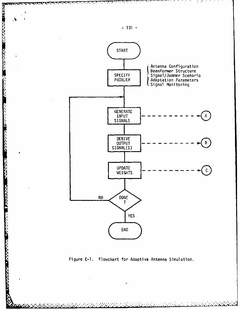
- 131 -

D Antenna Configurationj IBeamformer Structure

SPECIFY Signal/Jammer ScenarioPROBLEM Adaptation Parameters

Signal Monitoring

GENERATE

"'. INPUT

SIGNALS

,[" DERIVE--'i OUTPUT ,

ISIGNAL(S)

:.I I

UPDATE4 WEIGHTS

i

I NO DN

'YES

9

Figure E-1. Flowchart for Adaptive Antenna Simulation.

! , -. - . , -, ---.. ,.. ".. ' .. '-- - -.- ' -0"' -. ' -1: - - . " , . - - -: . -:- '''' -

W- 77 - -T-71

1 32 -

2. Signal/jammer arrival angle

3. Signal/jammer power

2. 4. Signal/jammer center frequency and bandwidth

-"

D. Adaptation parameters

1. Number of adaptation cycles

2. Adaptation constant

E. Signal (e.g. input, master output, slave output) to be stored for later

analysis.

All of these data are organized into disk files and thus made available for use by

various programs during the simulation or for reuse in subsequent runs.

The first step in the actual simulation is generation of the initial samples of

the input signals. This can be accomplished by a direct computation for.4;

sinusoidal signals since amplitude is known from the power specification and the

phase at any tap is known from the antenna/beamformer specifications, the

i1s signal frequency, and the initial (or prior-sample) phase. The process is more

difficult for wideband signals. These signals are derived by first generating a

white-noise sequence and then digitally bandpass filtering to obtain the desired

center frequency and bandwidth. In general, the sample values derived in this

fashion will not correspond exactly to the sample values needed at the antenna

elements since fractional-sample-interval delays are often encountered. A sinc

i ' :-,.',' .' - , .- '-. ---- " , . .. .. ...- -.- , ' " ",-".. . -.. , .--. -,.

- 133 -

interpolation is used to correct for this effect and provide accurate input samples

in the wideband case. The aggregate signal sample at each tap is just the sum of

the various signal and jammer samples derived for the tap. Separate signal

vectors are maintained for master and slave beamformers.

Once the signal vectors have been obtained for some sample instant, it is

straightforward to calculate the output signal or signals by forming the inner

product of a signal vector with the current weight vector. In the case of the

composite beamformer, both the master beamformer output and the slaved

beamformer output are required.

Weight updating is accomplished based upon the current signal vector and

the current adaptive array output. The weight recursion for the Frost ABF was

given in Eq. (2-17).

=After the new weight vector has been obtained, the next adaptation cycle

can begin. A check is made at this point to determine whether the prespecified

iV number of cycles has been completed. If so, the adaptation routine halts. If not,

the process of computing input samples, outputs, and new weight values

continues.

As the simulation progresses, data of interest are saved by transcribing to

disk files. The use of disk files allows large amounts of data to be saved and thus

supports lengthy adaptation experiments involving tens of thousands of

adaptation cycles. Additionally, the disk files provide convenient interfaces

between the simulation program and various data analysis programs.

h

-134-

C. Plotting or Antenna Responses

Two types of plots are typically used to characterize the response of an

adaptive antenna with some specified set of beamformer weights. One plot shows

the response to a unit-power test signal of specified frequency as the test-signal

angle of arrival is varied through, say, 360". This plot is usually termed a

"beampattern" and is useful in determining the relative response of the system to

jammers and desired signals. The second plot shows the response to a unit-power

test signal from a specified direction as the test-signal frequency is varied over

some range, generally from zero to half the sampling frequency. This plot is a

frequency-response characterization for the selected direction and is useful in

checking the effectiveness of jammer nulling and confirming the maintenance of

look-direction constraints. Both plot types are used most frequently to study

antenna response after the beamformer weights have converged (in the mean) to

the optimal solution for the environment under consideration. The plots may,

however, be plotted for any specified set of weights. A series of plots may be

generated to study, for example, the evolution of the antenna response as

adaptation occurs or the dynamics of the antenna response after convergence.

A flowchart of the procedure for generating and plotting antenna responses

is given in Figure E-2. The response plots are specified from the driver program,

which then starts the appropriate program for either a beampattern plot or a

frequency-response plot. Either program must first read the driver-specified

weight file and plot-parameter files from disk. The response for a given arrival

-135-

START

SPECIFYPATTERN

PLOT j

GI~--- ....[READ WEIGHTS]

COMPUTE(RESPOUSE

PLOTRESPONSE J

END

Figure E-2. Flowchart for Generationand Plotting of Antenna Responses.

-136-

direction and frequency is then found by forming the phasor sum of the weighted

tap voltages and computing the beamformer output power from the amplitude of

the sum. Repeated computations of this type give the response at enough

directions or frequencies to accurately characterize the antenna response. The

response is then plotted for study. A polar plot with a logarithmic (dB) radial

scale is usually preferred for beampattern plots, but a semilogarithmic cartesian

presentation sometimes serves well. A cartesian plot is used for the frequency-

response data, with frequency as the abscissa and power (in dB) as the ordinate.

D. Plotting of Input/Output Signals

Plots of input and output signals and their spectra are important in the

study of adaptive antenna performance. These plots are especially valuable in

investigations of signal cancellation. Cancellation effects that are difficult to

recognize in beampattern or frequency-response plots can be easily detected by

comparing input and output waveforms or spectra.

Input and output data are gathered during the course of simulation

experiments and written to disk files for later analysis and display. A number of

different signals (e.g. the desired signal, jammer signals, master beamformer

output, slaved beamformer output) may be collected to thoroughly characterize

beamformer behavior during various simulations. Plots of these data allow

comparisons to be drawn between different beamformers, different operating

4on

conditions, etc.

• -~~~~~....... ............... .... ,. ,....-....... ... ,... .... ,........ ,,........-...-,.

-137-

Figure E-3 diagram the event flow for production of input/output plots. If

spectral plots are elected, a DFT routine is entered to generate power spectra for

the selected signals. The DFT routine allows selection of transform size and

supports the computation of an average power spectrum over some specified

range of data samples. The power spectra are written to disk upon completion of

this computation. The plot program allows several signals or spectra to be

presented simultaneously for comparison. Waveform or spectral data are read

from specified disk files and plotted on separate axes with a common scale for

easy comparison.

APPROVED FOR PUBLIC RECEASEDISTRIBUTION UNLIMITED

to

CI

N - 138-

;STARTSPECTRA NO

:1 ___-Ye

~PLOT-- --- WAVE FORMS/

SPECTRA

END

Figure E-3. Flowchart for Generating andPlotting Input/Output Signals.

_ _ , .. . , - - , . , . ..- . ;.. . , .. . , .. . ., ,. - .,.. . ... . ... .,:-. . , - ,. . . . . .. . ,. . . .. ., ..

FILMED