Embed Size (px)
Citation preview

arX
iv:2
001.
1144
5v2
[as
tro-
ph.I
M]
14
Feb
2020
Draft version February 17, 2020Typeset using LATEX manuscript style in AASTeX62
IGRINS Slit-Viewing Camera Software
Hye-In Lee,1 Soojong Pak a,1 Gregory N. Mace,2 Kyle F. Kaplan,3 Huynh Anh N. Le,4
Heeyoung Oh,5 Chan Park,5 and Sungho Lee5
1School of Space Research, Kyung Hee University, 1732 Deogyeong-daero, Giheung-gu, Yongin-si, Gyeonggi-do, 17104,
Republic of Korea
2Department of Astronomy, University of Texas at Austin, Austin, TX 78712, USA
3SOFIA Science Center, NASA Ames Research Center, Moffett Field, CA 94035, USA
4Department of Astronomy, University of Science and Technology of China, Hefei, People’s Republic of China
5Korea Astronomy and Space Science Institute, Daejeon 34055, Republic of Korea
(Revised February 17, 2020)
Submitted to PASP
Abstract
We have developed observation control software for the Immersion GRating INfrared
Spectrometer (IGRINS) slit-viewing camera module, which maintains the position of
an astronomical target on the spectroscopic slit. It is composed of several packages that
monitor and control the system, acquire the images, and compensate for the tracking
error by sending tracking feedback information to the telescope control system. For effi-
cient development and maintenance of each software package, we have applied software
engineering methods, i.e., a spiral software development with model-based design. It
is not trivial to define the shape and center of astronomical object point spread func-
tions (PSFs), which do not have symmetric Gaussian profiles in short exposure (<4 s)

2 Lee et al.
guiding images. Efforts to determine the PSF centroid are additionally complicated
by the core saturation of bright guide stars. We have applied both a two-dimensional
Gaussian fitting algorithm (2DGA) and center balancing algorithm (CBA) to identify
an appropriate method for IGRINS in the near-infrared K-band. The CBA derives
the expected center position along the slit-width by referencing the spillover flux ratio
of the PSF wings on both sides of the slit. In this research, we have compared the
accuracy and reliability of the CBA to the 2DGA by using data from IGRINS com-
missioning observations at McDonald Observatory. We find that the performance of
each algorithm depends on the brightness of the targets and the seeing conditions, with
the CBA performing better in typical observing scenarios. The algorithms and test
results we present can be utilized with future spectroscopic slit observations in various
observing conditions and for a variety of spectrograph designs.
Keywords: Instrumentation: spectrographs — methods: data analysis, numerical —
techniques: spectroscopic
1. INTRODUCTION
Slit or fiber spectrographs are the most commonly used in modern astronomical spectroscopy. Since
a slit or a fiber tip on the focal plane collects photons for dispersion, the signal to noise ratio (S/N)
of a point target depends on the reliability of centering it in the collector. Studies by Shimono et al.
(2012) and Tamura et al. (2012) showed the importance of well defined relationship between a system
and the control software in the development of Prime Focus Spectrograph and the Fiber Multi Object
Spectrograph for Subaru Telescope. In the case of SpeX on the NASA Infrared Telescope Facility
(Rayner et al. 2003; Rayner 2017), the instrument control software consists of four components on
Bigdog, Guidedog, and Littledog computers. The Guidedog controls the infrared (IR) slit-viewing
camera (SVC) to monitor the spillover photons from the target on the slit or the off-slit guide star in
the field. Since the refraction index in IR bands is smaller than that in visible bands, the IR image
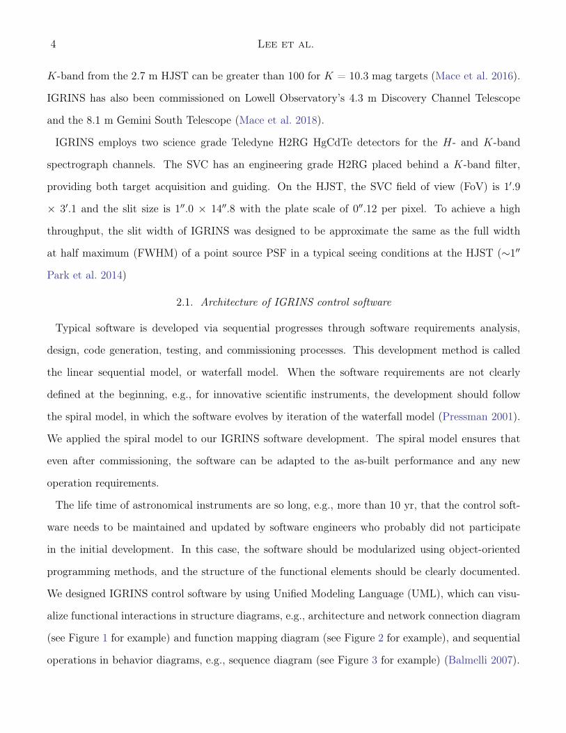
3
is less affected by the atmospheric turbulence and the IR guiding is more stable and efficient than in
the optical (Lacy et al. 2002; Rayner et al. 2003).
We have developed the Slit Camera Package (SCP) for operation of the Immersion GRating INfrared
Spectrometer (IGRINS) (Kwon et al. 2012; Park et al. 2014; Mace et al. 2016). IGRINS control soft-
ware was designed with numerous center-finding algorithms in accordance with software engineering
methods. There were a number of complications that had to be overcome, like saturated centers
and asymmetries of the point spread function (PSF) images in short exposures (<4 s) caused by
atmospheric turbulence. The asymmetric PSF profile can be a large fraction of a slit width. Ap-
propriate observation modes and scenarios can compensate for these properties and reduce slit-loss,
which means more science target flux on the spectral detectors and higher S/N spectra. We report
the performance of a guiding algorithm that has not been used with previous IR spectrographs, so
it can be useful for the future development of similar instruments.
In this paper, we describe IGRINS control software and the requirements of the SCP, including the
center balancing algorithm (CBA). Section 2 explains the control software architecture design and
the concepts of pointing and guiding for IR observations. In Section 3, we show the results with the
16 sample guide star images from the IGRINS SVC. We then discuss the performance test results in
Section 4, and discuss quantitative differences. Finally, we will summarize all of this work in Section
5.
2. OVERVIEW OF THE SCP
IGRINS is a compact and high-resolution (R = 45,000) near-IR, cross-dispersed, echelle spectro-
graph. In 2014 March, IGRINS had the first commissioning observations on the 2.7 m Harlan J.
Smith telescope (HJST) at McDonald Observatory (Park et al. 2014). The optical design of IGRINS
was carefully optimized to have high throughput. With simultaneous exposures in H- and K-bands,
IGRINS observes continuous wavelength spectra from 1.45 to 2.5 µm using a silicon immersion grating
(Jaffe et al. 1998; Marsh et al. 2007; Wang et al. 2010; Gully-Santiago et al. 2012), which was more
than 30 times the spectral grasp of the original CRIRES on the Very Large Telescope (Kaufl et al.
2004). The spectral S/N, per resolution element, of a point source observed with IGRINS in the
4 Lee et al.
K-band from the 2.7 m HJST can be greater than 100 for K = 10.3 mag targets (Mace et al. 2016).
IGRINS has also been commissioned on Lowell Observatory’s 4.3 m Discovery Channel Telescope
and the 8.1 m Gemini South Telescope (Mace et al. 2018).
IGRINS employs two science grade Teledyne H2RG HgCdTe detectors for the H- and K-band
spectrograph channels. The SVC has an engineering grade H2RG placed behind a K-band filter,
providing both target acquisition and guiding. On the HJST, the SVC field of view (FoV) is 1′.9
× 3′.1 and the slit size is 1′′.0 × 14′′.8 with the plate scale of 0′′.12 per pixel. To achieve a high
throughput, the slit width of IGRINS was designed to be approximate the same as the full width
at half maximum (FWHM) of a point source PSF in a typical seeing conditions at the HJST (∼1′′
Park et al. 2014)
2.1. Architecture of IGRINS control software
Typical software is developed via sequential progresses through software requirements analysis,
design, code generation, testing, and commissioning processes. This development method is called
the linear sequential model, or waterfall model. When the software requirements are not clearly
defined at the beginning, e.g., for innovative scientific instruments, the development should follow
the spiral model, in which the software evolves by iteration of the waterfall model (Pressman 2001).
We applied the spiral model to our IGRINS software development. The spiral model ensures that
even after commissioning, the software can be adapted to the as-built performance and any new
operation requirements.
The life time of astronomical instruments are so long, e.g., more than 10 yr, that the control soft-
ware needs to be maintained and updated by software engineers who probably did not participate
in the initial development. In this case, the software should be modularized using object-oriented
programming methods, and the structure of the functional elements should be clearly documented.
We designed IGRINS control software by using Unified Modeling Language (UML), which can visu-
alize functional interactions in structure diagrams, e.g., architecture and network connection diagram
(see Figure 1 for example) and function mapping diagram (see Figure 2 for example), and sequential
operations in behavior diagrams, e.g., sequence diagram (see Figure 3 for example) (Balmelli 2007).
5
IGRINS control software runs on the Instrument Control Computer, which is independent but
networked to both IGRINS and the telescope control system (TCS). It consists of the House Keeping
Package (HKP), the Data Taking Package (DTP), and the SCP. Figure 1 shows IGRINS software
architecture and the network connections (Rayner et al. 2003; Kwon et al. 2012). Components in
all packages were analyzed and designed by UML. In addition to the sequential operations, they do
threaded execution to avoid memory leak in the platform. The HKP controls and monitors the status
of the hardware components. The DTP takes spectral data, provides approved observing modes, and
controls the data flow and archiving. It also interacts with the calibration module via the HKP. The
SCP controls the SVC and communicates with the TCS. It performs an IR auto-guiding function
either by the off-slit guide star in the slit camera field or by the spillover photons from the target
on the slit (Rayner et al. 2003; Iseki et al. 2008; Landoni et al. 2012). The software was written in
Python 2.7 and used Tcl/Tk for graphic user interface (GUI) the elements on the environment of the
Macintosh operating system.
2.2. Operation Sequence
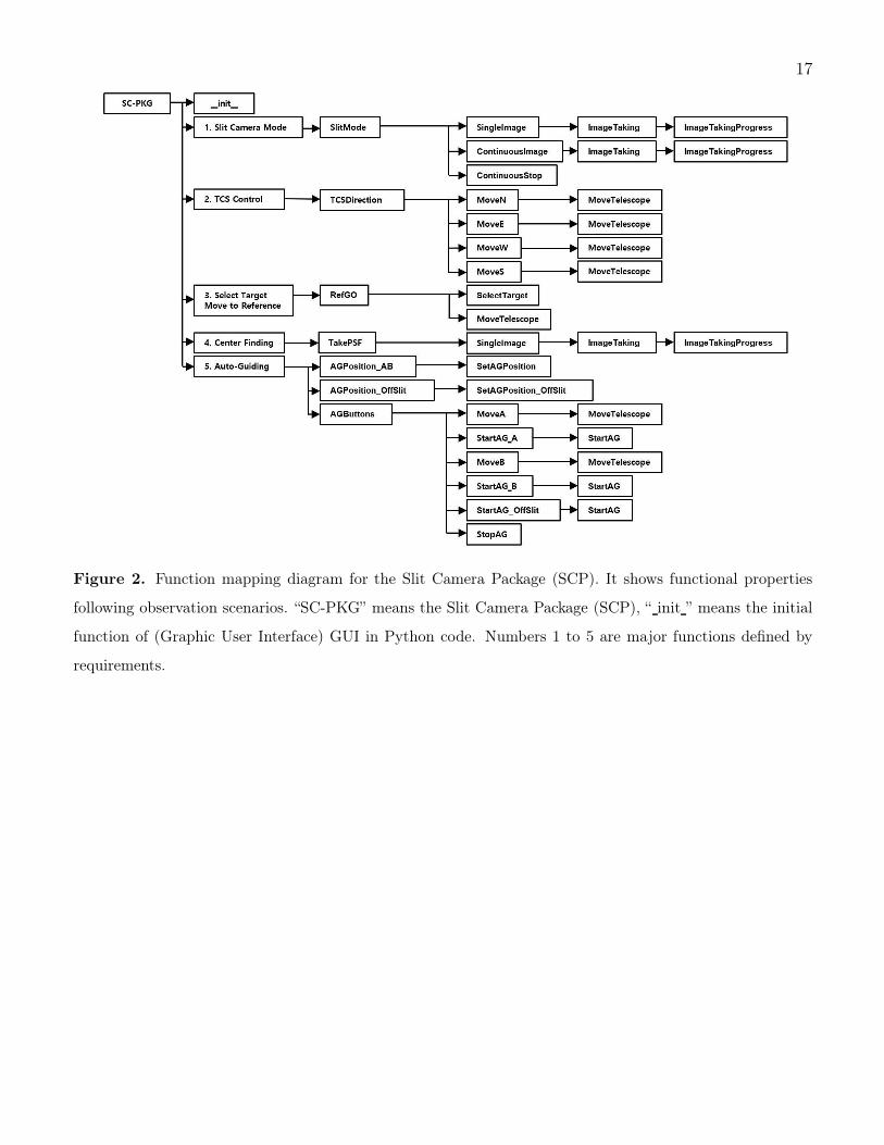
In Figure 2, we modeled every function and command using UML. Each required element is to be
a function code or command. We arranged the major functions in the GUI. Each functions can have
sub-functions, and some of the functions can be called by the major functions of high levels. We
deployed a sequence diagram for each operation (see example in Figure 3).
2.2.1. Boot-up and Shutdown
After the SCP opens a socket for internal connection to the DTP, it loads the initial coefficients
in the configuration file. The DTP and the SCP are connected with the science detector control
computers for each H2RG array. When the connections between the HKP and the DTP, the DTP
and the SCP, and the SCP and the TCS are ready, the SCP sends command to the Science Detector
Control Computer for Slit Camera (SDCS) to initialize the detector and to prepare for taking an
image. It also starts to get a current information of the TCS through TCP/IP. When all observation

6 Lee et al.
processes are complete, all packages sequentially exit alive threads and the GUI in the reverse order
of the boot-up processes.
2.2.2. Pointing and Guiding
The concepts of pointing in the telescope control include identifying the science target and setting
the target at the observing position, e.g., the spectroscope slit aperture (McGregor et al. 2000). We
defined a reference position (the green cross in Figure 4) which is near the slit in the SVC FoV
(Chen et al. 2012; McCormac et al. 2013). After confirming the target on the reference position, the
SCP finds the center of the target image and moves the telescope to place the target on the slit.
For faint or extended targets the center of the target is difficult to define and identify. In these
cases we use a guide star whose offset position from the target is accurately known. Placing the guide
star in the pre-set guide box defined from the offset (the pink box in Figure 4), we can efficiently and
effectively confirm the target on the reference position and move the target on the slit.
While IGRINS acquires spectroscopic observations with exposure times between 1.63 and 1800 s,
the SCP continuously takes the slit view images as Rayner et al. (2003) did for SpeX, and checks
the pointing by finding the center of the target on the slit or the guide star in the guide box. The
telescope tracking errors can be compensated for by periodically commanding the TCS to adjust
pointing. The pointing process is shown in the sequence diagrams in Figure 3.
2.2.3. Observing Mode
Infrared spectroscopy relies on periodically nodding the telescope pointing between the target and
the blank sky (Lacy et al. 2002; Rayner et al. 2003) to permit the subtraction of thermal background
emission from the telluric atmosphere, the telescope mirrors, and the instrument optics. To collect
the background data in the same observing conditions, observers need to be able to adjust telescope
pointing between spectroscopic frames.
We defined an A-box (the red box in Figure 4) for the target on the slit position and a B-box (the
cyan box in Figure 4) for sky observations. Both box positions are pre-determined by observers,
and the pointing can be performed by centering the target inside the boxes. When the target is at

7
the A-box, we can expect to take the data from the target. The reduction pipeline subtracts the
B-frame, which was taken with the target at the center of the B-box, from the A-frame. Note that
the B-box position on the slit camera FoV does not correspond to the blank sky. For observers to
check the blank sky position, the SCP shows a ghost B-box (the cyan dotted box filled of diagonal
lines in Figure 4) which is at the opposite side of the B-box.
For point source targets, observers can use a nod-on-slit mode, where both A-box and B-box are
on the slit. Unless the target is too faint, the pointing calibration is done by taking a target image
on the slit. In this mode, both A-frame subtracted by B-frame and B-frame subtracted by A-frame
can be combined in the reduction process.
For angularly extended targets, a nod-off-slit mode, in which the A-box is on the slit and the B-box
is out of the slit, should be used. If the target has a well-defined peak at the center, e.g., active
galactic nuclei, observers can use the target image on the slit to point. Otherwise, observers should
point the target by placing and centering the guide star at the guide box. By using the user-defined
script mode, with incremental offset values between the A-box and the guide-box, a slit-scan mode
can produce a three-dimensional data cube.
2.3. Center Finding Methods
When the target is placed on the slit, most of the target photons pass through and are then
collected by the spectrograph optics. The slit camera image contains only the spillover photons, but
the center of the PSF can be derived by fitting the spillover using the two-dimensional Gaussian
fitting algorithm (2DGA; Press et al. 2007). However, this maximum likelihood estimation can have
fatal biased errors when the peaked profile is blocked by the slit.
In the SCP, we developed a simple and robust CBA to define the center of the target. Assuming
the PSF is symmetric in the wings, the maximum throughput can be achieved when the spillover
photons in the slit width direction are balanced (Rayner et al. 2003; Landoni et al. 2012; Rayner
2017). When observers identify and confirm the target on the reference position (see Section 2.2.2),
the target image without any slit obstruction can be obtained. As shown in Figure 5, the SCP can
put virtual slit blocks at various offsets and simulate the slit-obstructed PSF images with which we

8 Lee et al.
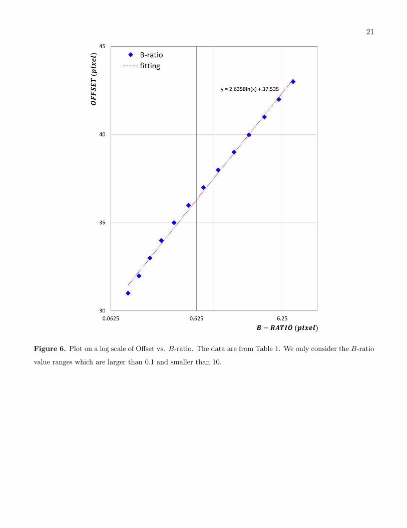
can derive the balance ratios (B-ratios) of the upper to the lower spillover flux values. Table 1 lists
simulated B-ratios from the sample images in Figure 5. Because the slit offset values and the B-ratios
are mapped linearly in Figure 6, the SCP can effectively estimate the offset position of the target
from the measured B-ratio during observations.
In order to explain the CBA and the way of IGRINS software design, we show the flowchart (see
Figure 7) and the sequence diagram (see Figure 8) to make the balance table. Using the flowchart
we can analyze the requirements and derive the solution model. Based on the flowchart, we included
interactions with other software packages and designed the sequence diagram using UML.
2.4. Auto-guiding Mode
After the SCP creates the balance table from the target image on the reference position, observers
can move the target into the A-box and begin acquiring spectra. The SCP takes the point target
image on the slit, and calculates the energy ratios (B-ratio) of the lower to the upper parts of the
slit. Applying the measured B-ratio value to the model relationship, the autoguider can move the
target onto the center of the slit width by sending the position offset commands to the TCS. In the
auto-guiding mode, this process repeats, while the DTP takes spectroscopic data.
3. PERFORMANCE TEST
3.1. Sample Data
The test data were taken at the McDonald 2.7 m telescope during IGRINS commissioning runs in
2014 March, May, and July. We selected 618 SCP frames from 16 point sources (5 < mK < 9 mag)
with various environmental conditions (see Table 2). In our sample frames, the positions of the point
sources were distributed around the center of the slit width direction (Iseki et al. 2008). Since the
shortest integration time of the array readout electronics is 1.63 s (Jeong et al. 2014), bright targets
in good seeing conditions were easily saturated at this short test integration time.
3.2. Expected Target Position
When the target was on the reference position, both centers of the target and another off-slit point
source were measured by the 2DGA. This method is reliable without slit mask obstructions. After

9
moving the target onto the slit, we measured the center of the off-slit point source by 2DGA and
derived the expected target position from the offset between the two sources. Figure 9 shows the
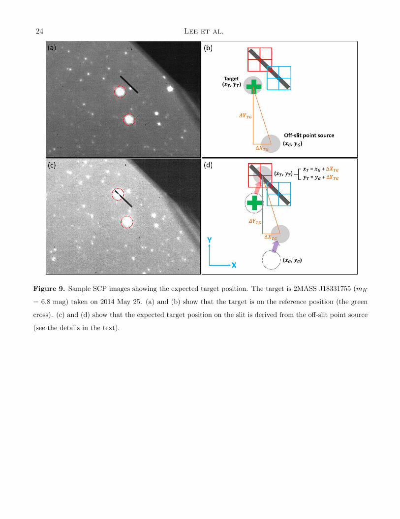
coordinates and definitions of position parameters. The red dotted circles of (a) and (c) are target
and off-slit point source. In (b), xT and yT are the center values of the target. xG and yG are the
center values of the off-slit point source. These center positions were derived by 2DGA. From the
center values, we got a distance ∆XTG and ∆YTG (the orange triangle and text). After the target
goes into the slit such as the blue and purple arrow (in case of A box, the red box) in (d), we inferred
the expected center of the target (xT=xG+∆XTG, yT=yG+∆YTG). The center of the target with slit
mask obstruction was measured by both 2DGA and CBA. Note that the definitions of the centers
from both 2DGA and CBA would be slightly different with saturated or non-symmetrical PSF.
3.3. Center Finding Errors
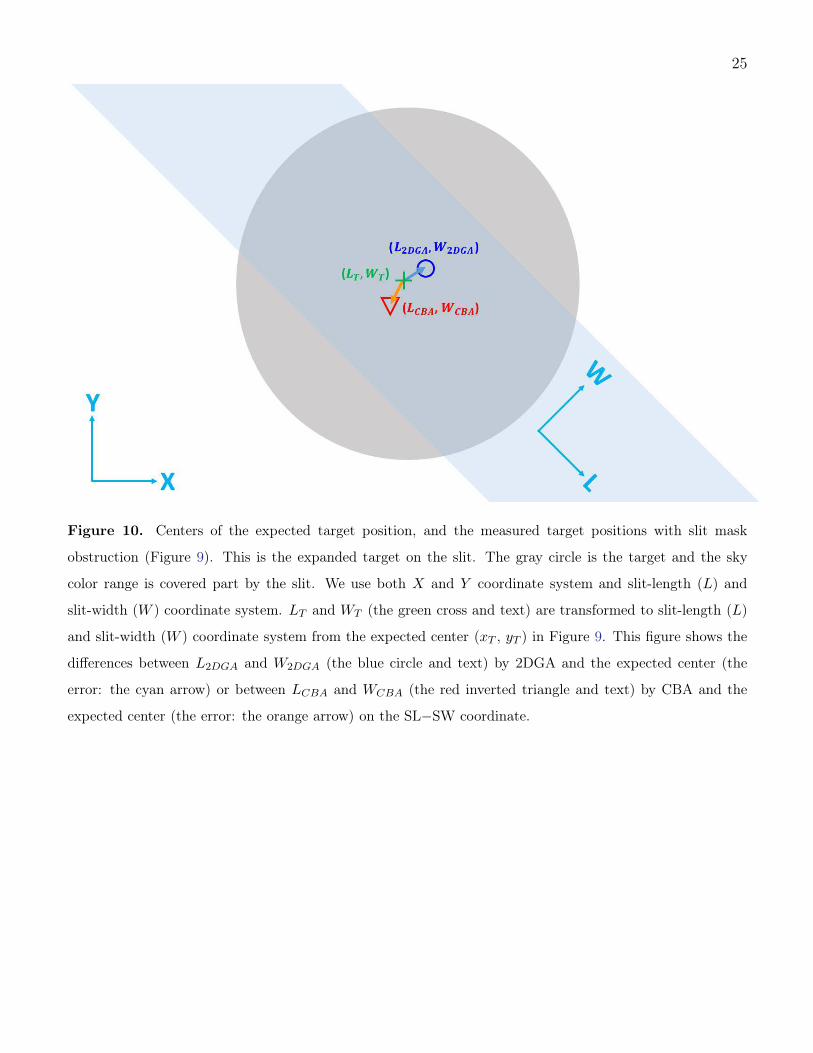
Since the center finding errors are mixed in the elements of X and Y , we have transformed the image
data from the X and Y coordinate system in the array format to the slit-length (L) and slit-width
(W ) coordinate system (see Figure 10). Since the pointing along the W direction is more critical for
minimizing slit-loss, only the slit-width direction component was considered (Iseki et al. 2008). The
measured target centers, with slit mask obstruction, from the 2DGA and the CBA, subtracted by
the expected target center, i.e., (∆W2DGA = W2DGA −WT ) and (∆WCBA = WCBA −WT ) were the
errors of the center finding algorithms (see Figure 10).
4. RESULT AND DISCUSSION
4.1. Characterizing Error Patterns
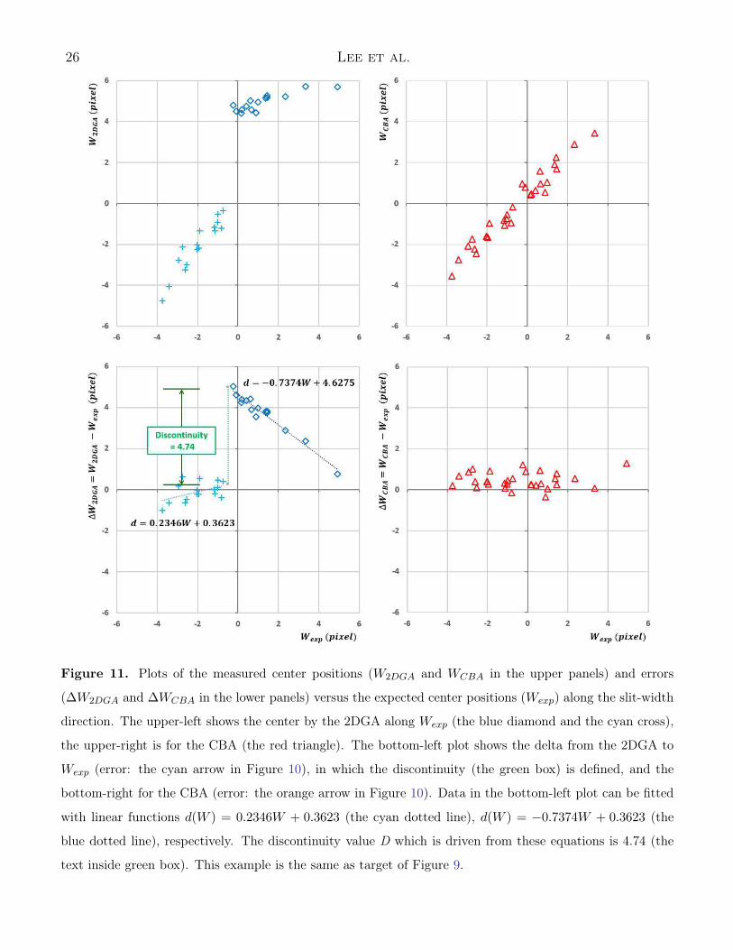
Figure 11 shows the measured center positions (W2DGA and WCBA) and errors (∆W2DGA and
∆WCBA) versus the expected center positions (WT ). The distribution of the errors in the slit co-
ordinate, as well as the root mean square (RMS) of the errors, can be compared to evaluate the
performance of the center finding algorithms.
The errors from the 2DGA in Figure 11 show a noticeable discontinuity pattern around the center.
This problem arises when the FWHM of the target PSF is smaller than the slit width. Figure 5

10 Lee et al.
shows the slit-blocked PSF profiles, which the 2DGA may misidentify the edge of the slit aperture as
the center of the PSF profile. When the target is near this discontinuous position, the auto-guiding
can be very unstable and begin jumping between the two slit edges. To quantize this fatal feature,
we modeled a simple linear discontinuous function, d(W ),
d(W ) =
a0 + a1W, when W ≤ c
b0 + b1W, when W > c
(1)
Where a0, a1, b0, b1, and c values derive from the minimum χ-squared value. We define a disconti-
nuity value, D, as follows:
D = |a0 + a1c− (b0 + b1c)| (2)
The above discontinuity value is another way of showing the performance and stability of the center
finding algorithms. Figure 11 shows that error (∆WCBA) distributions from the CBA do not have
any discontinuity features.
4.2. Errors in Various Conditions
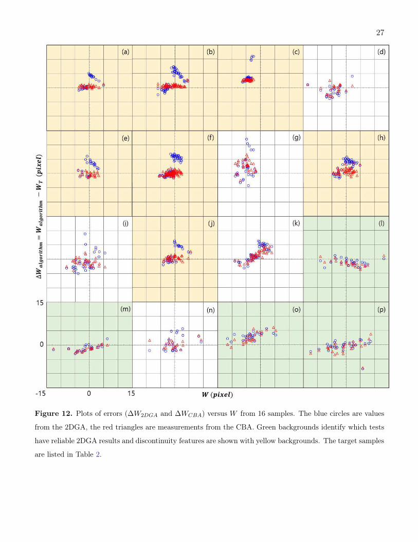
In this section, we compare the performance of the 2DGA and the CBA in various observing
conditions. Figure 12 shows plots of errors for all our data from the 16 targets. The error distribution
patterns are different for each center finding algorithm, and depends on the target brightness and
seeing conditions. Table 2 lists RMS values from the 2DGA and the CBA, and the discontinuity
values from the 2DGA. The CBA does not display discontinuities.
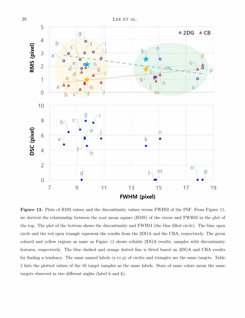
We plotted the RMS values and the discontinuity values as a function of the FWHM of the PSF
(see Figure 13). With smaller FWHM values, the RMS values from the 2DGA are larger, while
those from the CBA are somewhat smaller. To find the relationship between the error distribution
patterns in Figure 12 and the RMS and discontinuity values in Figure 13, we marked with the yellow
background color on both figures. When the FWHM is large (with the green background color), the
RMS differences between the 2DGA and the CBA are not significant. The CBA outperforms the
11
2DGA when the FWHM is small, which is also when the discontinuity feature in the 2DGA becomes
4-8 pixels (∼0.5-1 slit width).
Figure 14 shows the performances as a function of the target magnitude. Fainter targets have less
overflow flux on the sides of the slit, which decreases the reliability of the 2DGA to fit the peak using
the fainter wings of the PSF. The RMS values from the 2DGA are slightly decreasing as the brightness
of the target increases. For very bright targets, e.g., mK < 6 mag, four out of five samples do not
have discontinuity features because saturation causes large FWHM values. The CBA performs well,
even at low flux, because the ratio of overflow flux is minimally impacted by a decrease in overall
flux. The RMS values from the CBA show different trends, performing slightly better for fainter
targets, as we see in Figure 13.
5. CONCLUSIONS
We have applied software engineering methods, i.e., the model-based design and the spiral devel-
opment process, to IGRINS control software development. To maximize the number of collecting
photons in the spectrograph slit, we made CBA in addition to the typical 2DGA. Applying both al-
gorithms to commissioning observations, in various observing conditions at McDonald Observatory,
we showed that they both perform well in poor seeing conditions. Since very bright point sources
are easily saturated at the peak, the size of the PSF becomes bigger even in good seeing conditions
and this limits the effectiveness of the 2DGA. When the FWHM is comparable to the slit width, the
2DGA algorithm shows a discontinuity near the slit center because most of the stellar flux passes
through the spectrograph slit. In typical observing conditions, the CBA finds the center of the
slit-blocked image better than the 2DGA.
ACKNOWLEDGEMENT
This work was supported by the National Research Foundation of Korea (NRF), grant No.
2017R1A3A3001362, funded by the Government of the Republic of Korea (MSIP). Hye-In Lee and
Huynh Anh N. Le were supported by the BK21 Plus program through the NRF funded by the Min-
istry of Education of Korea. This work used the Immersion Grating Infrared Spectrometer (IGRINS)
12 Lee et al.
that was developed under the collaboration between the University of Texas at Austin and the Korea
Astronomy and Space Science Institute (KASI) with the financial support of the US National Science
Foundation under Grant AST-1229522 of the University of Texas at Austin, and of the Korean GMT
Project of KASI. The IGRINS software Packages were developed based on the contract between
KASI and Kyung Hee University. We thank the anonymous referees for their critical comments to
improve this paper. We appreciate Dr. John Kuehne of the McDonald Observatory, Dr. Moo-Young
Chun and Dr. Jae-Joon Lee of KASI, and Prof. Sungwon Lee and Mr. Bong-Yong Kwon of KHU
for contributing to this research. We also thank Prof. George Parks and Ms. Elaine S. Pak for
proofreading this manuscript. This paper includes data taken at the McDonald Observatory of the
University of Texas at Austin.
REFERENCES
Balmelli, L. 2007, Journal of Object Technology, 6,
149
Chen, L., Zhang, Z., & Wang, H. 2012, Proc.
SPIE, 8451, 84512K
Gully-Santiago, M., Wang, W., Deen, C., & Jaffe,
D. T. 2012, Proc. SPIE, 8450, 84502S
Iseki, A., Tomono, D., Tajitsu, A., Itoh, N. &
Miki, S. 2008, Proc. SPIE, 7019, 70192D
Jaffe, D. T., Keller, L. D., & Ershov, O. A. 1998,
Proc. SPIE, 3354, 201
Jeong, U., Chun, M.-Y, Oh, J. S., et al. 2014,
Proc. SPIE, 9154, 91541X
Kaufl, H. U., Ballester, P., Biereichel, P., et al.
2004, Proc. SPIE, 5492, 1218
Kwon, B., Kang, W., Cho, E., et al. 2012, KNOM
Review, 15, 2, 25
Lacy, J. H., Richter, M. J., Greathouse, T. K.,
Jaffe, D. T., & Zhu, Q. 2002, PASP, 114, 153
Landoni, M., Riva, M., Zerbi, F. M., et al. 2012,
Proc. SPIE, 8451, 84512X
Mace, G., Kim, H., Jaffe, D. T., et al. 2016, Proc.
SPIE, 9908, 99080C
Mace, G., Sokal, K., Lee, J.-J., et al. 2018, Proc.
SPIE, 10702, 107020Q
Marsh, J. P., Mar, D. J., & Jaffe, D. T. 2007,
ApOpt, 46, 3400
McCormac, J., Pollacco, D., Skillen, I., et al. 2013,
PASP, 125, 548
McGregor, P. J., Conroy, P., Harmelen, J. v., &
Bessell, M. S. 2000, PASA, 17, 102
Park, C., Jaffe, D. T., Yuk, I.S., et al. 2014, Proc.
SPIE, 9147, 91471D
Press, W. H., Teukolsky, S. A., Vetterling, W. T.,
& Flannery, B. P. 2007, Numerical Recipes: The
Art of Scientific Computing (3rd ed.; New York:
Cambridge Univ. Press)
13
Pressman, R. S. 2001, Software Engineering: A
Practitioner’s Approach (5th ed.; New York:
McGraw-Hill)
Rayner, J. T. 2017, SpeX Observing Manual (Hilo,
HI: NASA Infrared Telescope Facility) rev. 3
Rayner, J. T., Toomey, D. W., Onaka, P. M., et al.
2003, PASP, 115, 362
Shimono, A., Tamura, N., Sugai, H., & Karoji, H.
2012, Proc. SPIE, 8451, 84513F
Tamura, N., Takato, N., Iwamuro, F., et al. 2012,
Proc. SPIE, 8446, 84460M
Wang, W., Gully-Santiago, M., Deen, C., Mar, D.
J., & Jaffe, D. T. Proc. SPIE, 7739, 77394L

14 Lee et al.
Table 1. Balancing table
of SS433
Index Offset B-ratio
(pixel)
1 31 0.1001
2 32 0.1332
3 33 0.1782
4 34 0.2438
5* 35 0.3451
6 36 0.5054
7 37 0.7527
8* 38 1.1320
9 39 1.7160
10 40 2.5750
11 41 3.8983
12* 42 5.7586
13 43 8.3880
Note—Sample data were taken on 2014 May 24. “Offset” is the distance between a virtual slit and the
center of the target. “B-ratio” is the balancing ratio of the slit-width direction between up and down from
the virtual slit. The virtual-slit-blocked PSF images and the PSF profiles of Index 5, 8, and 12 (marked
with “*” symbols) are shown in Figure 5.

15
Table 2. Comparison of Results from 2DGA and CBA algorithms
Index Target Mag (K) FWHM (pixel)2DGA CBA
Label
Rms DSC Rms
20140525 2MASS J18331755 6.8 8.06 2.40 4.74 0.55 a
20140526 Serpens2 8.6 8.40 2.95 6.40 0.51 b
20140524 Serpens15 7.0 9.24 2.50 6.75 0.22 c
20140711 SR4 (V* V2058 Oph) 7.5 9.36 1.81 0 1.53 d
20140713 HD155379 6.5 9.58 2.13 5.68 0.74 e
20140524 SS433 8.2 9.59 3.00 5.51 0.66 f
20140712 HD155379 6.5 9.65 3.88 7.90 1.90 g
20140712 GSS32 7.3 9.74 2.11 4.56 1.00 h
20140711 HD155379 6.5 10.22 3.07 7.65 1.31 i
20140525 V2247Oph 8.4 10.78 2.58 5.54 0.75 j
20140526 GSS32 7.3 14.07 2.53 4.55 1.80 k
20140708 HIP5131 5.3 14.69 1.16 0 1.09 l
20140525 25 Oph 5.5 15.10 2.53 5.50 1.34 n
20140709 HIP95560 5.6 17.85 1.03 0 1.77 o
20140709 HIP93580 5.3 18.21 1.86 0 2.09 p
Note—“Index” is a list of commissioning dates. “2DGA” and “CBA” represent two-dimensional Gaussian
fitting algorithm and center balancing algorithm, respectively.
“FWHM” is taken through 2DGA on the reference position. “Label” is a list of FWHM arranged in a large
order which is used Figure 12.

16 Lee et al.
Figure 1. IGRINS control software architecture and network connection. The pointing and guiding parts
are enclosed within the red solid line. The packages developed for IGRINS control software system are in the
gray boxes: the House Keeping Package (HKP), the Slit Camera Package (SCP), the Data Taking Package
(DTP), the Quick Look Package (QLP), the Pipeline Package (PLP), and Observation Preparation Package
(OPP). Other packages from the observatory or from the off-the-shelf are in the white boxes: the Telescope
Control System (TCS), Science Detector Computer for Slit-camera (SDCS) Array Control Package, Science
Detector Computer for K-band (SDCK) Array Control Package, and Science Detector Computer for H-band
(SDCH) Array Control Package (Kwon et al. 2012). We used Unified Modeling Language (UML) (Visual
Paradigm 15.1, Visual Paradigm International Ltd.) to make this diagram.
17
Figure 2. Function mapping diagram for the Slit Camera Package (SCP). It shows functional properties
following observation scenarios. “SC-PKG” means the Slit Camera Package (SCP), “ init ” means the initial
function of (Graphic User Interface) GUI in Python code. Numbers 1 to 5 are major functions defined by
requirements.

18 Lee et al.
Figure 3. Sequence diagram for target pointing. These processes show that “3. Select Target Move to
Reference” of major functions in Figure 2. The sequential order numbers are labeled from 1 (read information)
to 11 (confirm target): 1. The Slit Camera Package (SCP) requires information from the Telescope Control
System (TCS). 2. The SCP displays the TCS information (R.A. and decl.). 1 and 2 continue until finishing
the current observation. 3. The observer finds a target by “Single” mode. 4. Then, the SCP communicates
with SDCS for taking a data. 5. After finding the target, the SCP calculates the center of the target. 6-9.
The observer decides and commands whether “on-slit guiding” or “off-slit guiding”, the guiding star moves
into a pre-defined box (A-box or guide box). 10. The observer confirms to identify the target through “Single”
or “Continuous” mode. The auto-guiding process follows after this pointing process.

19
Figure 4. Slit Viewer part of Graphic User Interface (GUI) of the Slit Camera Package (SCP). The green
cross is the reference position, the red and cyan boxes are pre-defined A and B position of on the slit. The
pink box is a guiding position for off-slit mode. The cyan dotted box filled of diagonal lines means blank
sky position. The user can turn on or off the guide box and blank sky box through checking “Use Guide
Position” and “Show Sky” in the GUI, respectively.

20 Lee et al.
Figure 5. Sample point source images overlapped by virtual slits. The target is SS433 (mK = 8.2 mag)
taken on 2014 May 24. As Figure 10, it converts X and Y coordinate into slit-length and slit-width. (“SW-
position” is slit-width direction, this is a relative position value (pixel) in pre-defined box on the reference
position.) The right plots show the one-dimensional profile along the slit width direction (marked with the
white dashed line on the left image). Inside the right plots, the “Offset” value shows the offset position of
the virtual slit in pixel units. “B-ratio” is the spillover energy ratios of upper to lower parts from the virtual
slits.
21
Figure 6. Plot on a log scale of Offset vs. B-ratio. The data are from Table 1. We only consider the B-ratio
value ranges which are larger than 0.1 and smaller than 10.

22 Lee et al.
Figure 7. Flowchart to make a balance table. The part of the pointing process at the reference position is
included in the process of making balance table.
23
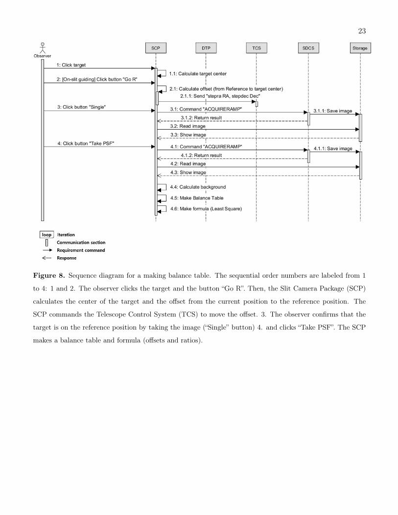
Figure 8. Sequence diagram for a making balance table. The sequential order numbers are labeled from 1
to 4: 1 and 2. The observer clicks the target and the button “Go R”. Then, the Slit Camera Package (SCP)
calculates the center of the target and the offset from the current position to the reference position. The
SCP commands the Telescope Control System (TCS) to move the offset. 3. The observer confirms that the
target is on the reference position by taking the image (“Single” button) 4. and clicks “Take PSF”. The SCP
makes a balance table and formula (offsets and ratios).
24 Lee et al.
Figure 9. Sample SCP images showing the expected target position. The target is 2MASS J18331755 (mK
= 6.8 mag) taken on 2014 May 25. (a) and (b) show that the target is on the reference position (the green
cross). (c) and (d) show that the expected target position on the slit is derived from the off-slit point source
(see the details in the text).
25
Figure 10. Centers of the expected target position, and the measured target positions with slit mask
obstruction (Figure 9). This is the expanded target on the slit. The gray circle is the target and the sky
color range is covered part by the slit. We use both X and Y coordinate system and slit-length (L) and
slit-width (W ) coordinate system. LT and WT (the green cross and text) are transformed to slit-length (L)
and slit-width (W ) coordinate system from the expected center (xT , yT ) in Figure 9. This figure shows the
differences between L2DGA and W2DGA (the blue circle and text) by 2DGA and the expected center (the
error: the cyan arrow) or between LCBA and WCBA (the red inverted triangle and text) by CBA and the
expected center (the error: the orange arrow) on the SL−SW coordinate.
26 Lee et al.
Figure 11. Plots of the measured center positions (W2DGA and WCBA in the upper panels) and errors
(∆W2DGA and ∆WCBA in the lower panels) versus the expected center positions (Wexp) along the slit-width
direction. The upper-left shows the center by the 2DGA along Wexp (the blue diamond and the cyan cross),
the upper-right is for the CBA (the red triangle). The bottom-left plot shows the delta from the 2DGA to
Wexp (error: the cyan arrow in Figure 10), in which the discontinuity (the green box) is defined, and the
bottom-right for the CBA (error: the orange arrow in Figure 10). Data in the bottom-left plot can be fitted
with linear functions d(W ) = 0.2346W + 0.3623 (the cyan dotted line), d(W ) = −0.7374W + 0.3623 (the
blue dotted line), respectively. The discontinuity value D which is driven from these equations is 4.74 (the
text inside green box). This example is the same as target of Figure 9.
27
Figure 12. Plots of errors (∆W2DGA and ∆WCBA) versus W from 16 samples. The blue circles are values
from the 2DGA, the red triangles are measurements from the CBA. Green backgrounds identify which tests
have reliable 2DGA results and discontinuity features are shown with yellow backgrounds. The target samples
are listed in Table 2.
28 Lee et al.
Figure 13. Plots of RMS values and the discontinuity values versus FWHM of the PSF. From Figure 12,
we derived the relationship between the root mean square (RMS) of the errors and FWHM in the plot of
the top. The plot of the bottom shows the discontinuity and FWHM (the blue filled circle). The blue open
circle and the red open triangle represent the results from the 2DGA and the CBA, respectively. The green
colored and yellow regions as same as Figure 12 shows reliable 2DGA results, samples with discontinuity
features, respectively. The blue dashed and orange dotted line is fitted based on 2DGA and CBA results
for finding a tendency. The same named labels (a to p) of circles and triangles are the same targets. Table
2 lists the plotted values of the 16 target samples as the same labels. Stars of same colors mean the same
targets observed in two different nights (label h and k).

29
Figure 14. Plots of RMS values and the discontinuity values versus the apparent K magnitude. As Figure
13, we derived the relationship between the RMS of the errors and K magnitude in the plot of the top. The
plot of the bottom shows the discontinuity and K magnitude (the blue filled circle). The blue open circle
and the red open triangle represent the results from the 2DGA and the CBA, respectively. The green colored
regions shows reliable 2DGA results as same as Figure 12. The blue dashed and orange dotted line is fitted
based on 2DGA and CBA results for finding a tendency. The same named labels (a to p) of circles and
triangles are the same targets. Table 2 lists the plotted values of the 16 target samples as the same labels.
Stars of same colors mean the same targets in the other days (label h and k in the green box, which means
same target).