Geological Survey of India

Central Region

Seminary Hills, Nagpur, India

Base Document

1st

National Working Group Meeting

4t h

and 5t h

Oc t obe r, 2010

IGCP 582

TROPICAL R IVERSTROPICAL R IVERS HYDRO-PHYSICAL PROCESSES,

IMPACTS, HAZARDS AND M A N A G E M E N T

Edited by Snigdha Ghatak

Vivek P Malaviya N V Venkatraman

FOREWORD

The 1st meeting of the International Geological Correlation Programme

(IGCP) –now called, ‘International Geoscience Programme’ is a platform for

eminent geoscientists to collaborate and exchange ideas, experiences in the field

of earth sciences. IGCP is a unique collaboration between International Union of

Geological Sciences (IUGS) and United Nations Educational, Scientific and

Cultural Organisation (UNESCO), for last three decades working in global

environment, natural resources, natural hazards etc.

IGCP activities in India is monitored by the Indian National Committee

(INC). INC is headed by Director General, Geological Survey of India (GSI) as

its ex-officio Chairman. INC also has members from ONGC, NGRI, AMD,

WIHG, BARC, CGWB, CWC, SINP, etc.

IGCP-582 in particular is a consortium of professionals to interact on

hydro-physical processes, hazards and management of Tropical Rivers. IGCP-

582 consists of professionals from geoscientific organisations like NGRI, NIH,

WIHG, ISM and academicians from University of Lucknow and CEPT

University. This group will work on various aspects of tropical river system

with special emphasis on the Holocene period of earth’s history.

This compilation of work provides a glance of the experience of the

distinguished experts in this subject field, who will work together for the next 4

years in the identified areas.

I take this opportunity to convey my best wishes to the newly selected

NWG members and wish the IGCP-582 all success in its initiatives and

endeavour.

FROM THE DESK OF THE DEPUTY DIRECTOR GENERAL AND HOD, CENTRAL REGION

The Geological Survey of India, as the nodal agency for Indian National

Committee (INC), implements IGCP Projects in India. IGCP 582 on Tropical

Rivers is one such programme that is being taken up this year to continue till

2014 in India. It gives me immense pleasure to know that the 1st National

Working Group (NWG) meeting for the prestigious IGCP 582 which has

tremendous societal values is being organized at Geological Survey of India,

Central Region, Nagpur.

I look forward to active participation of the geoscientists and

brainstorming sessions from this 1st NWG meeting. I extend my best wishes

to all the participants in this regard.

I extend my sincere thanks to Chairman, IGCP, INC, Chairman, IGCP

582 and Member Secretary, IGCP, INC for providing logistics and

infrastructural support. I also wish to place on record, the sincere initiative on

the part of Convener, IGCP 582 , NWG members and officials associated with

IGCP 582 secretariat at GSI,CR for arranging the meeting and bringing out

a volume within such a short time span. I am confident that the deliberations

will lead to fruitful contributions to the success of IGCP 582 Project.

INTERNATIONAL GEOSCIENCE PROGRAMME– 582  

TROPICAL RIVERS: HYDRO‐PHYSICAL PROCESSES, IMPACTS, HAZARDS AND MANAGEMENT 

(2009 ‐ 2014) 

INDIAN NATIONAL WORKING GROUP  Chairman, INC for IGCP:  Director General, Geological Survey of India  Member Secretary, INC for IGCP: 

 K. Balasubramaniam, Director, International Division 

 Chairman, IGCP582: 

 Dr. K. Rajaram, Deputy Director General, Op. Maharashtra, Head Mission II, Central Region, Geological Survey of India   

Convener:  Dr. (Mrs.) Snigdha Ghatak, Sr. Geologist, Geodata Division, GSI, CR  

Members:  

Dr. Ahmad S. Masood , Scientist ‐ ‘G’, Head Paleoclimate Group, NGRI  Shri N.V. Venkatraman, Senior Geologist, Geological Survey of India, Central Region  Dr. Rakesh Kumar , Scientist – F, Surface Water Hydrology Division, National Institute of Hydrology, Roorkee   Dr. M.S. Bodas, Senior Geologist, Project: Landslides, Geological Survey of India, Central Region, Pune  Dr. Pradeep Srivastava, Scientist – C, Sedimentology Group, Wadia Institute of Himalayan Geology, Dehradun   Dr. Sreemati Gupta, Senior Geologist, LHIM & EPE Division, Geological Survey of India, Pushpa Bhavan,  New Delhi   

Prof. Vinay Kumar Srivastava, Department of Applied Geophysics, Indian School of Mines, Dhanbad   Prof. Rameshwar Bali, Centre of Advanced Study in Geology, University of Lucknow, Lucknow   Dr. Vivek P. Malviya, Mineralogist, Mineral Physics Lab, Geological Survey of India, Central Region, Nagpur   Prof. Ajay K. Katuri, Faculty of Planning and Technology (CEPT), Center for Environmental Planning and Technology (CEPT) University, Ahmedabad, Gujarat  Shri Manoj Kumar Shukla, Assistant Geologist (Gr.‐I), Op: UP & UK, Quaternary Geology Project, Geological Survey of India, Lucknow  Shri Rajesh Kumar Senior Geologist, Geodata Division, Geological Survey of India, CHQ, Kolkata  Shri N.R. Mohapatra, Senior Geologist, Op. WB‐AN, Geological Survey of India, Eastern Region, Salt Lake, Kolkata          

 

Contents  

Page no.

Section I: Short papers Tropical rivers: hydro-physical processes, impacts, hazards and management (IGCP 582)…………………….. …..Rajiv Sinha, Edgardo M. Latrubesse,

1

Jose C. Stevaux, Zhongyuan Chen

Morphological modeling within Hoogly estuary, Indian Sunderbans: A framework for coastal zone management……….Snigdha Ghatak, Goutam Sen

5

Flood hazard modeling and flood risk assessment for a river basin…………………………………………………………..Rakesh Kumar

14

Assessment of urban flood in light of a river-front development project……………………… Ajay Kumar Katuri, Cees Van Westen, Naveen

23

Kumar Chikara

Study of drainage patterns as observed on remote sensing images over Jharia- Raniganj coal field of Eastern India………………………….V. K. Srivastava

43

Section II: Abstracts Soils and their mineral formation as tools in provenance, climate change and Geomorphological Research…………… …………………………..D.K. Pal

49

Impact and hazards of flooding in Mumbai …..…………….....M Chandradas 50

Process and forms of mountainous tropical river systems - example from Kerala state, South India……………. …………S. Manju and s. Anirudhan

52

Quaternary geology of Central India…………………………… M.P Tiwari 54

Late Quaternary fluvial history of the Upper Brahmaputra Valley, Northeastern India………………………………………………………………..N.R.Ramesh

55

Section I

1

TROPICAL RIVERS: HYDRO-PHYSICAL PROCESSES, IMPACTS,

HAZARDS AND MANAGEMENT (IGCP 582)

Rajiv Sinhaa, Edgardo M. Latrubesseb, Jose C. Stevauxc, Zhongyuan Chend

aGeosciences Group, Indian Institute of Technology Kanpur, Kanpur 208016, INDIA bDepartment of Geography and the Environment, University of Texas at Austin, USA

cUniversidade Guarulhos-Pr. Tereza Cristina, 1 – Centro, Guarulhos, SP, Brazil dEast China Normal University, Shanghai 200062, China

Introduction

River systems are considered as the economic engine in tropical regions; they have a central

role in electricity production, and sustain the bulk of agricultural production and other high-value

economical activities based on natural resources extraction (mining, fishing, timber). At the same time

they can also be drivers of natural disasters such as floods, bank erosion and rapid channel migration.

The most recent example of this is the Indus floods in Pakistan which affected 14 million people and

has devastated 1/5th of the country. Another major river disaster occurred in the Kosi river basin in

north Bihar and Nepal affected more than 3 million people when the river avulsed by more than 120 km

in August 2008 and the new channel, ~22km wide, carried 144,000 cusecs of discharge inundating

large areas (Sinha, 2009).

Tropical rivers draining the wet and wet-dry tropics with annual rainfall totals more than

700mm/year occur in a variety of geologic-geomorphologic settings: (a) orogenic mountains belts, (b)

Sedimentary and basaltic plateau/platforms, (c) Cratonic areas, (d) Lowland plains in sedimentary

basins and (e) Mixed terrain (Latrubesse, et al., 2005). The size of the river basins varies from 104 to

6x106 km2 and all of them show clear high but variable peak discharges during the rainy season and a

period of low flow when rainfall decreases. Some tropical rivers show two flood peaks, a principal and

a secondary one, during the year. Large tropical rivers in different parts of the world have drawn

particular attention and a range of subjects have been investigated including geomorphology,

sedimentological and hydro-sedimentary processes, flood and paleoflood hydrology and tectonic/

fluvial processes relationships. However, bearing in mind the large extent of the tropical regions and

the size of the rivers themselves, the knowledge base of the tropical rivers is still limited.

2

Keeping this in view, the ongoing IGCP 582 project on tropical rivers is focused on three

principal research themes: 1) analysis of past and present behavior on key hydrophysical indicators of

climate change (e.g. mean discharges, flood frequency, drought occurrence, sediment transport,

geomorphic processes), and within the environmental systems (soil degradation, desertification,

ecotope distribution); 2) study of spatial and temporal human impacts on land use (agriculture,

deforestation, river engineering, mining) and related changes to water resources, considering the

countries’ policy and institutional framework; and 3) establishment of a set of methods on river

management to decrease hydro-physical impacts of global change, flood disasters and direct impacts

by river engineering and mining. This paper presents a synthesis of the major issues related to tropical

rivers and challenges of research in this area.

Challenges of tropical river research

Large populations in developing economies, chaotic growth of urban areas and a sharp increase

in water and power demands are some of the common problems in all tropical countries. The resources

available and management strategies adopted to tackle geomorphic disasters, however, may be entirely

different from country to country. These differences eventually affect the overall economic growth of

the country. For example, Brazil, with a total of 8.5 million km2 of area and around 190 million people,

is considered as one of largest agricultural producer in the world because of a widespread agricultural

area and intensive water management practices. On the other hand, millions of people in India live on

rather rudimentary agriculture and face scarce availability of ground and surface water. This has

obviously resulted in a much lower rate of growth in the agricultural sector in India and has also

affected the water and power demands in many parts of the country.

Similarly, the overall increasing trends in sediment load in river basins of Colombia such as the

Madgalena River are attributed to a range of anthropogenic influences including decrease in forest

cover and increase in agricultural and pasture. In Argentina and Bolivia, the impact of land use changes

in historic time scale is also dramatic and has been affecting some of the most productive fluvial basins

of the world in terms of sediment production such as the Pilcomayo and Bermejo rivers. The

environmental disaster is repeating now with the destruction of the Chaco and the Sub Andean forest

along the socially and economically underdeveloped parts of these countries where flow some of the

most avulsive rivers of the world. Another major concern can be identified in flood disasters while

comparing different countries and regions. In Asia, the occurrence of floods is recurrent and

3

catastrophic and even though some of the largest rivers of the world drain through South America,

floods are not as much significant as in Asia and some basins of Africa

Human interference with the river systems has affected the natural flow conditions of tropical

rivers in many ways. Construction of dams and barrages on major rivers affects the entire river system

manifested as aggradation or degradation in certain reaches and alteration of natural ecosystem because

of changes in supply of nutrients and sediments. Water pollution, produced by the influx of large

amounts of mercury in the rivers, however, was significant, particularly along the Tapajos river basin

affecting mainly a few minor tributaries. At present, gold extraction by garimpeiros is scarce and

declining. Today mining in tropical countries of Africa is a huge and unknown environmental disaster.

As a good example we can use Angola, where a good part of the fluvial systems has been affected by

mining. The tropical rivers of New Guinea such as the Fly basin have been severely affected by mining

extraction for decades. The Fly is a medium sized river and its sediment load was significantly altered

by mining waste, increasing from 85 to more than 100 million tons/year (Milliman et al., 1999). Other

estimations suggest annual additions of ~50 million tons of sediments through mining waste, out of

which ~3% is transferred to the floodplain (Dietrich et al., 1999).

The IGCP 582 project: plan of action

The overall scope of the IGCP 582 project is to provide an integrated assessment of long-term

direct impacts of climate variability and human-induced change and management of tropical rivers

basins by identification, quantification and modeling of key hydro-geomorphologic indicators during

the past and present times. The potential impacts of global change on fluvial systems and of their socio-

economic implications will also be analyzed.

Research plan

Activity 1: Multidisciplinary Data Base on tropical rivers: Reports, data and spatial information (digital

maps and images) will be available trough a web site

Activity 2: Reconstruction of climates and past environment using indicators of global changes

Activity 3: Analysis of hydro-geomorphologic parameters of Global change and mechanism of

sediment routes

4

Activity 4: Analysis and compilation of recent flood disasters, investigation of the causative factors and

debate on the efficacy of the existing flood control measures

Knowledge dissemination

A series of international meetings will be organized during the project duration. At least one

intercontinental meeting will be organized to involve the majority of the participant researchers. With

this objective we will encourage the inclusion of our IGCP meetings inside largest international

meetings. Several meetings are planned to be organized in different parts of the world and they will

announced form time to time to enable the researchers to participate and interact.

Concluding remarks

The IGCP is a unique platform that facilitates the interaction among the researchers across the

globe. In tropical regions, it is a fact that generalizations are frequently encountered when comparing

the different developing countries or “tropical” countries. The IGCP 582 project would contribute

significantly towards understanding of tropical river systems in terms of their societal relevance as this

will address the issues of river management and human intervention as well as the flood disasters which

are often interconnected. The IGCP would facilitate the sharing of experiences of river management

among the researchers from different parts of the globe and would therefore contribute directly to the

Society.

References

Dietrich, W.; Day, G. and Parker, G. 1999. The Fly river, Papua New Guinea: inferences about Ruver

Dynamics, floodplain sediemntation and fate of sediemnt. In: Miller, A.J. and Gupta, A. (Eds.),

Varieties of Fluvial Form, J. Wiley & Sons, 345-376.

Milliman, J.D., Farnsworth, K.L. and Albertin, Ch. 1999. Flux and fate of fluvial sediments leaving

large islands in the East Indies. Journal of Sea Research, 41: 97-107.

Sinha, R. (2009). The Great avulsion of Kosi on 18 August 2008. Current Science, 97(3), 429-433.

Latrubesse, E.M., Stevaux J.C. and Sinha, R. (2005) Tropical Rivers. Geomorphology, 70/3-4, 187-

206.

5

MORPHOLOGICAL MODELING WITHIN HOOGLY ESTUARY, INDIAN SUNDERBANS: A FRAMEWORK FOR COASTAL ZONE MANAGEMENT

Snigdha Ghataka, Goutam Senb

aGeological Survey of India, Central Region, Nagpur bSchool of Ocenaographic Studies, Jadavpur University, Kolkata

Abstract

The southern sea facing islands of the Indian part of the Ganges- Brahmaputra delta is constantly under

threat due to natural causes and anthropogenic interventions. This demands implementation of viable

management plan backed by scientific reasoning. In this backdrop, coastal area morphological

modeling of Sagar Island located within Hoogly estuary was taken up utilizing map, imagery and tide

gauge computed relative sea level rise rate for the period between 1942 and 2001. Spatio-temporal

correlation based model was utilized to determine continuous variation of coastal configuration with

varying relative sea level rise (RSLR) scenario. Present study indicates, with higher sea level rise

greater amount of erosion is evident. 2.8mm/yr. of RSLR rate could be determined within Hoogly

estuary which is not on the higher side. A good match between the projected configuration of Sagar

Island and map data for same year determines the effectiveness of the model at least at decadal to sub

decadal scale.

Key words: Ganges Brahmaputra delta, relative sea level rise, spatio-temporal correlation, morphological modeling

Introduction

The West Bengal part of the Ganges-Brahmaputra delta, popularly known as the Sundarban delta, is a

system where intricate estuarine and coastal processes are influenced by adjacent marine, terrestrial and

meteorological systems and the dynamic interface amongst the three. Being the center of population

growth, coastal sea, ponds/wetlands, estuarine islands in this area are to sustain the negative impact

caused by society’s commercial, recreational, and residential activities. Additionally, natural forcing

like sea level rise or climate change is a prime issue of concern for this vulnerable tract. Presently, this

deltaic system is facing degradation due to natural and anthropogenic causes. Degradation of this

6

littoral tract is manifested in terms of frequent embankment failures, submergence & flooding, beach

erosion, siltation within embayment, saline water intrusion in the agricultural field etc (Hazra et al.

2002).

In the above perspective, viable coastal zone management options are to be adopted based on scientific

approach retaining socio-economic use of the coastal zone complying with preservation of resources

and nature values. Knowledge and understanding of coastal morphodynamic behaviour as well as

middle to long-term developments therein is essential in this respect. Lack of data pertaining to this

coast makes the task all the more difficult than expected and restricts proper estimation of impacts to be

caused by the different coastal variables.

The present study is aimed at predicting evolution of Sagar Island located at the mouth of Hoogly

estuary by a set of physical mathematical model through extrapolation of observed morphological

behaviour of erosion-accretion. The long term goal of this study is to identify the coupling amongst the

coastal processes and mainly two dimensional evolutions (shoreline change) of the form of deltaic

island system of West Bengal with special reference to sea level rise which in turn is guided by climate

change. This study is carried out so that a greater degree of certainty can be achieved while applying

the output as a blue print for the coastal managers and planners for this vulnerable niche.

Geological and Geomorphological setup:

Ganges-Brahmaputra delta is located at the northern apex of Bay of Bengal. Quaternary outbuilding of

the fine silt to mud dominated, macrotidal, lobate (Boyd et al., 1992) Sundarban delta took place

following depositional regression of the sea during Middle Holocene. With a tidal range of about 3.5 to

5m in the estuaries and complex network of estuaries, creeks and islands, this delta is a classic example

of tide dominated one and harbors the largest single continuous tract of mangrove forest. The Ganges-

Brahamaputra delta is represented by a low-lying flood plain covering more than 90,000 sq. km in India

and Bangladesh and grades into a more extensive sub-aqueous delta and deep sea fan complex. The

main sediment sources for the delta and the fan are the Ganges and Brahamaputra rivers, with a yearly

discharge of 1x109 t, with 80% of discharge occurring during the four months of SW Indian monsoon

(Coleman, 1969).

7

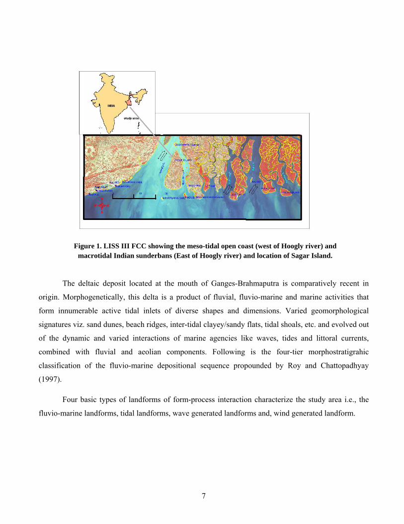
The deltaic deposit located at the mouth of Ganges-Brahmaputra is comparatively recent in

origin. Morphogenetically, this delta is a product of fluvial, fluvio-marine and marine activities that

form innumerable active tidal inlets of diverse shapes and dimensions. Varied geomorphological

signatures viz. sand dunes, beach ridges, inter-tidal clayey/sandy flats, tidal shoals, etc. and evolved out

of the dynamic and varied interactions of marine agencies like waves, tides and littoral currents,

combined with fluvial and aeolian components. Following is the four-tier morphostratigrahic

classification of the fluvio-marine depositional sequence propounded by Roy and Chattopadhyay

(1997).

Four basic types of landforms of form-process interaction characterize the study area i.e., the

fluvio-marine landforms, tidal landforms, wave generated landforms and, wind generated landform.

Figure 1. LISS III FCC showing the meso-tidal open coast (west of Hoogly river) and macrotidal Indian sunderbans (East of Hoogly river) and location of Sagar Island.

8

Table 1. Morphostratigraphy of the study area. (Source: Roy and Chattopadhyay, 1997).

Sundarban deltaic coast Age

Active estuarine deposit

Channel bar, intertidal flat and abandoned creek with or without mangroves, no oxidation effect of sediments

Older estuarine deposit

Interdistributary supratidal flat

Upper Holocene

Ancient estuarine deposit

Interdistributary stabilized supra-tidal flat Middle Holocene

Sagar Island:

Sagar Island is located at the mouth of the Hoogly estuary at the western extremity of the West

Bengal part of Sundarban delta. Sagar Island used to be a part of the single continuous stretch of

mangrove ecosystem prior to 1811. The reclamation of this fragile island was initiated thereafter as it

served as a source of revenue to British colonial government. The island became almost settled within

next 125 years. According to the 1991 census the population of the island was 1,49,222 with a decadal

growth of 39.9%. The natural processes like sea level rise, tidal action, current, wave etc. aided by

anthropogenic interventions have resulted into accelerated rate of erosion of the coastal stretch of the

island. Historical records indicate submergence of the Kapil Muni Temple, a significant cultural

landmark created at the southern tip of Sagar Island for couple of times in the recent past

(Bandyopadhyay, 1997). Apart from these the construction of Farakka dam upstream of the river

Ganges has affected the sediment budget and other physical variables for this estuary (Basu, 2001).

Materials and methods:

Data integration in time series using GIS (MapInfo) and image processing (ERDAS Imaging)

methodologies for Sagar island has been carried out using multi dated maps and imagery. Two types of

data sources utilized for the present work include raster data and rate of relative sea level rise data. The

raster data defines the initial condition for modeling for the three islands and includes 1942-SOI

toposheet, survey year: 1921-23, 1973, 1971– SOI toposheets survey year: 1967-68,1968-69, 1989-

LISS II FCC, 2001-LISS III digital data. Trend of shoreline changes is determined for Sagar Island

through overlay analysis of the high tide line (HTL) between the above mentioned time frames.

9

Quantitative change detection analysis is carried out on the vectorised data set to estimate the nature

and quantum of erosion and accretion for the islands. Limited ground truth input on HTL has been

incorporated after field studies for the year 2000, 2001 for Sagar Island. Field traverses pertaining to

physical identification of the zones of erosion and accretion in the year 2001 corroborate well with the

zones of erosion and accretion while comparing 2001 and 1988 data.

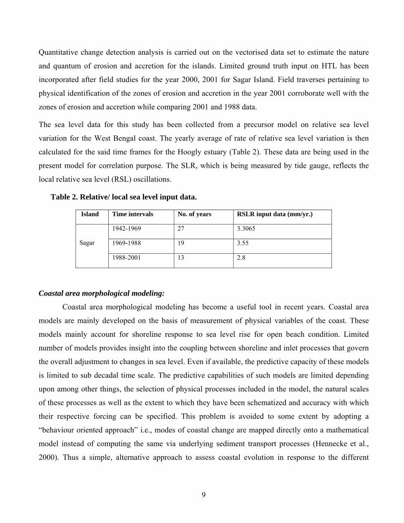
The sea level data for this study has been collected from a precursor model on relative sea level

variation for the West Bengal coast. The yearly average of rate of relative sea level variation is then

calculated for the said time frames for the Hoogly estuary (Table 2). These data are being used in the

present model for correlation purpose. The SLR, which is being measured by tide gauge, reflects the

local relative sea level (RSL) oscillations.

Table 2. Relative/ local sea level input data.

Island Time intervals No. of years RSLR input data (mm/yr.)

1942-1969 27 3.3065

1969-1988 19 3.55

Sagar

1988-2001 13 2.8

Coastal area morphological modeling:

Coastal area morphological modeling has become a useful tool in recent years. Coastal area

models are mainly developed on the basis of measurement of physical variables of the coast. These

models mainly account for shoreline response to sea level rise for open beach condition. Limited

number of models provides insight into the coupling between shoreline and inlet processes that govern

the overall adjustment to changes in sea level. Even if available, the predictive capacity of these models

is limited to sub decadal time scale. The predictive capabilities of such models are limited depending

upon among other things, the selection of physical processes included in the model, the natural scales

of these processes as well as the extent to which they have been schematized and accuracy with which

their respective forcing can be specified. This problem is avoided to some extent by adopting a

“behaviour oriented approach” i.e., modes of coastal change are mapped directly onto a mathematical

model instead of computing the same via underlying sediment transport processes (Hennecke et al.,

2000). Thus a simple, alternative approach to assess coastal evolution in response to the different

10

coastal processes including the role of sea level rise is also evaluated. (Thom and Roy, 1998; IPCC,

1996; Bakkar and De Vriend, 1995).

In the present study a statistical spatio-temporal correlation based model was developed

correlating sea level scenario and change of coastal configuration (Ghatak and Sen, 2004). The

evolution of Sagar Island in the past years (about 60 years for Sagar i.e., 1942-2001) around a common

reference point i.e., the centroid of the first base year, is estimated by considering rate of radial

shifts/change in the consecutive base years (say, for Sagar island it is 1969,1988,2001) in terms of

erosion and accretion. Spatial data of each intersecting data points between the radial line and each base

year HTL polygons are retrieved. Statistical correlation of rate of sea level change and rate of radial

change both spatially and temporally are incorporated into the GIS environment by applying a

functional relationship. Here, spatial as well as temporal data of positions are considered for correlation

analysis to understand the impact of one location on the dynamic process at other locations. Rationale

behind this hypothesis lies in the fact that hydrodynamics of river and sea is influenced by regional as

well as local constraints. As a result of this, impact is felt at adjacent regions. The degree of impact

again varies with positions from the zone of influence and so does the scenario for temporal changes.

The projected output reflects the configuration the island is likely to attain with a particular sea level

rise in the presence of set of other variables that were effective in the said time frame. Thus indirectly a

coastal form-process approach is adhered to where the dynamics of sediment transport or deposition

from one point to the other over a space of years is ultimately reflected in its form. The best correlated

points, best correlated sea level value and rate of change are cast under the shield of a composite

algorithm for Sagar Island to arrive at the projected outputs of the island configuration of the three

islands at a desired SLR scenario. Three sea level rise scenarios are initially considered for Sagar island

(including the maximum and minimum possible RSLR scenario for this region). This analysis is further

carried out to find out the projected configuration of the islands under most suitable relative sea level

rise (RSLR) scenario for a particular time interval by determining least area or shape deviation between

projected data of a year (projected from a base year) with the particular HTL of the same year as

available in the map. This predicted data is either projected from the previous base year, in case of

forecast situation or projected from next base year in case of hind cast situation with respect to a

particular base year.

Results:

Data analysis in the GIS platform reveals that the overall area of Sagar Island has decreased

between the years 1942 to 2001 with an initial decreasing trend of total area between 1942 to

1988 followed by an increasing trend between 1988 and 2001. The southern sector of Sagar

Island has been under the constant threat of erosion in the said time frame. The sites and rates of

erosion and accretion are not constant in different intervals of the said time frame. At the eastern

half of the island, south of Chemaguri Gang accretion is active and stabilization of the shoal by

mangrove growth is taking place, while at the northeastern part significant erosion has taken

place. The southern sea facing part of the island near Dublat, Kapil Muni’s temple, significant

erosion has taken place in the model time frame.

The initial estimate on the projected output of the island with these three different sea level rise

rates (viz. 3mm/yr., 3.5mm/yr., 4mm/yr.) after five years (2006), ten years (2011) and twenty

years (2021), projecting the same from 2001 shows that with increasing sea level accelerated

erosion or maximum percentage area loss will occur (2.68% with RSLR of 4mm/yr.). Estimation

of both shape and area change between the projected output and the original data set is carried out

through GIS query using three different RSLR scenario viz. 3mm, 3.5mm, 4mm/yr. Area change

is determined by measuring total area deviation between the projected year and reference year

and shape change is determined by estimating total deviation in area of the projected data set in

and outside the reference year. This is carried out to determine the order by which the projected

configuration moves toward the dynamic equilibrium configuration for that reference year. The

Chemaguri Gang

Figure 2. Area change of Sagar Island.

12

dynamic equilibrium configuration is achieved through continuous readjustment of the coast to the

environmental changes over the geological/historical periods in the regional and environmental

setting. The least deviation in total area or area deviation with respect to shape change provide

comparatively accurate sea level rise rates for different time frames assuming that erosion and

accretion are the effect of relative sea level rise for this region in the presence of other short-term

coastal variables. Using the above mentioned RSLR it is seen that 3.5mm/yr RSLR between 1942-

1969, 1969-1989 and 3mm/yr RSLR during 1989-2001 both for fore cast and hind cast situations

provide least deviation in comparison to the available maps of that particular year. Further fine-

tuning of data for RSLR is achieved by introducing smaller variation of the RSLR values for

particular time period and calculating the least deviation between projected and observed

configuration. This provides a suitable RSLR of 2.8mm/yr. for 1989-2001, 3.4mm/yr for 1969-1988

and 3.15mm/yr for 1942-1969. A good correlation between the projected and map data determines

the effectiveness of the model at least at decadal scale.

Conclusions:

Use of this type of coastal area morphological model is advantageous as very restricted type of

data (topographic maps and imagery, aerial photo and SLR data) can be utilized to provide

modeling outcomes. Moreover, the dynamics of sediment transport or deposition from one locale to

the other through space and time are indirectly considered into the model as the shoreline position

reflects the dynamic equilibrium condition through continuous adjustments to the environmental

changes over the geological/historical periods in the regional and environmental setting. The whole

approach of the study including new type of modeling method adds a new dimension for providing

the scientific background for formulating coastal zone management plans. The present knowledge

base with further research in these directions is expected to open up new vistas. This work is a

contribution to IGCP-582 project.

Acknowledgements:

The authors express their gratitude and thanks to Prof. A.D. Mukhopadhyay, Ex-Vice

Chancellor Vidyasagar University, India and Prof. S. Hazra, Director, School of Oceanographic

Studies, Jadavpur University, India, Dr. P. Sanyal, Retd. Addl. Chief Conservator of Forest, W.B,

India and Shri. B. K Saha, Retd. Dy. Director General, Marine Wing, Geological Survey of India,

for the constant encouragement and help rendered during carrying out this work.

13

References:

Bakkar, W.T. and de Vriend, H.J., 1995. Resonance and morphological stability of tidal basins. Marine Geology,126,5-18.

Bandopadhyay, S., 1997. Coastal erosion and its management in Sagar Island, South 24 Parganas, West Bengal. Indian Journal of Earth Sciences, 24(3-4), 51-69.

Basu, S.R., 2001. Impact of man on environment: Some cases of concern. In: Singh, L.R., (eds.), Professor R N Dubey Foundation Allahabad, 68p.

Boyd, R., Dalrymple, R. and Zaitlin, B.A., 1992. Classification of clastic coastal depositional environments. Sedimentary Geology, 80, 139-150.

Coleman, J.M., 1969. Brahamaputra river channel processes and sedimentation. Sedimentary Geology, 3, 129-139.

Ghatak, S. and Sen, G.K., (2004). Deltaic shoreline evolution in response to sea level rise. Third Indian National conference on Harbour and Ocean Engineering, 2004, National Institute of Oceanography, Goa, v 1, 139-147.

Hazra, S, Ghosh T, Dasgupta, R and Sen G, 2002. Sea level and associated changes in the Sunderbans. Science and culture, 68 , 9-12, 309-321.

Hennecke, W.G. and Cowell, P.J., 2000. GIS modeling of impacts of an accelerated rate of sea-level rise on coastal inlets and deeply embayed shorelines. Environmental Geosciences, 7(3), 137-148.

Intergovernmental Panel on Climatic Change (IPCC), 1996. Climate change 1995. The Science of Climate Change, Cambridge University Press, 572p.

Roy, R.K. and Chattopadhyay, G.S., 1997 Quaternary Geology of the environs of Ganga delta, West Bengal and Bihar. Indian Journal of Geology, 69(2), 177-209.

Thom, B.G., and Roy, P.S.,1998. Sea level rise and climate: Lessons from the Holocene. In: Pearman, G.I., (ed.), Greenhouse-Planning for climate change. Melbourne: Commonwealth Scientific and Industrial Research (CSIRO), Division of Atmospheric Research, 177-188.

14

FLOOD HAZARD MODELING AND FLOOD RISK ASSESSMENT FOR A RIVER BASIN

Rakesh Kumar

National Institute of Hydrology, Roorkee-247667, Uttarakhand, India

rk18p@yahoo.co.in and rakesh@nih.ernet.in

Abstract

In recent years the number and scale of water related disasters, flood in particular has been increasing.

The losses from floods often offset years of hard-won social and economic development. The problem

is further expected to be aggravated with the phenomena of climate change. Therefore, mitigation and

managing of flood hazards has become a priority for alleviating poverty, ensuring socio economic

progress, preserving our eco-systems and ensuring the gains of development. The paper presents

procedure for flood hazard modeling and flood risk zoning for a river basin. Floods of various return

periods have been estimated using the L-moments approach. Rating curves have been developed

employing the Artificial Neural Network and the least squares techniques. Depth of flooding,

inundation for various return periods and risk associated with the flooding have been simulated using

the HEC-RAS package. The flood inundation simulated by the HEC-RAS has been compared with the

flood inundation mapped using the satellite data.

Key Words : Flood hazard, Hydrologic Modeling, L-moments, Flood risk zoning.

Introduction

Flood is the most frequent natural disaster claiming loss of life and property compared to any other

natural disaster. About one-third of all losses due to nature’s fury are attributed to floods. On an

average floods claim a loss of more than 50 billion US dollars per year and 40000 victims per year in

the last decades of the twentieth century in the world (Berga, 2000). In India also, floods are the most

frequently faced natural disasters. As reported by Central Water Commission (CWC) under Ministry of

Water Resources, Government of India, the annual average area affected by floods is 7.563 million ha.

This observation is based on the data for the period 1953 to 2000 published in Indian Water Resources

15

Society (IWRS, 2001) with variability ranging from 1.26 million ha in 1965 to 17.5 million ha in 1978.

On an average floods have affected about 33 million persons during 1953 to 2000 and average annual

damage due to floods is about IRs. 46 billion. There is every possibility that this figure may increase in

future due to rapid growth of population and increased encroachments of the flood plains for habitation,

cultivation and other activities (Kumar et al., 2005).

Some of the important policies on flood management have been described by Kumar et al. (2005).

Various types of structural as well as non-structural measures have been envisaged to reduce the

damages in the flood plains in India. Construction of embankments, levees, spurs, etc. have been

implemented in some of the states. The total length of constructed embankments is 16800 km and

drainage channels are of 32500 km. A total of 1040 towns and 4760 villages are currently protected

against flood. Barring occasional breaches in embankments, these have provided reasonable protection

to an area of about 15.07 M ha. A large number of reservoirs have been constructed and these

reservoirs have resulted in reduction of intensity of floods. The non-structural measures such as flood

forecasting and warning are also being adopted. The flood forecasting and flood warning in India

commenced in 1958, for the Yamuna River in Delhi. It has evolved to cover most of the flood prone

interstate river basins in India. The Central Water Commission has established a flood forecasting

network for 70 rivers basins covering 18 States/Union Territories. The forecasts are issued at about 175

stations. Out of these 145 stations are for river stage forecasts and 28 for inflow forecasts to the

reservoirs. A Working Group of National Natural Resources Management System (NNRMS, 2002)

standing committee on water resources for flood risk zoning of major flood prone rivers considering

remote sensing input was constituted by the Ministry of Water Resources in 1999. The working group

recommended flood risk zoning using satellite based remote sensing with a view to give thrust towards

implementation of flood plain zoning measures. There is a need for taking more effective structural and

non-structural measures of flood management and flood damage reduction based on long term reliable

data, advance analyses and modelling procedures and antecedent rainfall forecasting using information

based on radar, satellite based instrumentation and high resolution Numerical Weather Prediction

(NWP) models. It also necessitates capacity building for implementation of these measures and

bridging the gaps between the developed advance and robust procedures and their field applications.

16

Definitions of Terms

The definitions of terms (i) flood inundation map, (ii) flood hazard map, (iii) flood risk zone map and

(iv) flood plain zoning map used in the study are described below.

Flood inundation map

A flood inundation map provides information about the areal extent of inundation for a reach of a river

during a flood event when the flood water in the river overtops its banks and leads to the flooding of

adjoining areas or flood plains. The flood inundation map for a reach of river may be prepared by

demarcation with physical inputs i.e. by demarcating the various locations of the flood plains which get

inundated during a particular flood, by hydraulic/hydrologic modelling and using the satellite data.

Flood hazard map

A flood hazard map provides information about the return period associated with the areal extent of

inundation for a reach of a river. The flood hazard maps are prepared delineating areas subjected to

inundation by floods of various magnitudes and frequencies. These maps may serve as important tools

in proper flood plain management. It is necessary that the area flooded by a particular flood is shown

by suitable colour scheme or designs on the map. In addition, explanatory notes, tables and graphs may

also be provided with flood hazard maps to facilitate their use.

Flood risk zone map

A flood risk zone map provides information about the risk associated with the damages caused or losses

resulting from a flood event in a particular area or flood risk zone. Preparation of flood risk zone map

incorporates the financial aspects and provides the actuarial inputs for flood insurance plans and for

other purposes.

Flood plain zoning map

A flood plain zoning map categorizes various zones based on administrative legislations for planning

and development of the flood plains for various purposes such as agricultural activities, play fields,

industrial areas and residential areas etc. Preparation of flood plain zoning maps takes into

consideration the inputs from flood inundation, flood hazard and flood risk zone maps.

17

Methodology

The methodology for flood hazard modeling and flood risk zoning for a reach of a river basin is briefly

described as follows. The objective of the study are: (i) to develop L-moments based flood frequency

relationships using the annual maximum peak flood series and the partial duration series for the

gauging sites of the river reach, (ii) to develop rating curves for the gauging sites of the river reach, (iii)

to prepare flood inundation maps for the river reach, (iv) to prepare flood hazard maps for the river

reach, (v) to prepare flood risk zone maps for the river reach and (vi) to predict flood inundation and

flood hazard areas for various stages of river flow.

In the study, risk is defined as the probability of occurrence of a flood at least once during

successive years of design life. The return period for which a structure should be designed is computed

based on the risk acceptable. Risk acceptable depends upon economic and policy considerations. If for

a time invariant hydrologic system the probability of occurrence of an event, x, greater than the design

event, xo, during a period of n years is P, then the probability of non-occurrence, Q is 1-P. The

probability that x will occur at least once in the n years i.e. the risk of failure, R is: R = 1-(1-1/T)n ;

where, R is the risk, T is the return period for which the structure should be designed, and n is the

design life of the structure (Robson & Read, 1999). Using the above formula, the return period T can be

determined for a given R (acceptable risk) during a period of time in years (n). The flood corresponding

to this T is estimated and routed through the river reach for estimation of the water surface profile and

inundation mapping. The expression of risk mentioned above may be extended to incorporate other

variables related to losses due to floods, which can be defined as functions of return period (T). The

flow chart illustrating the general terminology of flood inundation mapping, flood hazard mapping,

flood risk zone mapping and flood plain zoning is shown in Fig. 1.

Analysis and Results

In the study, flood frequency analysis has been carried out using the L-moments approach (Hosking &

Wallis, 1997; Kumar & Chatterjee, 2005; Kumar et al., 2003). For identifying the robust frequency

distribution for the respective gauging sites, L-moment ratio diagram and Zdist statistic criteria have

been adopted. Table 1 gives the Zdist statistic values for seven sites of the study area. The values of the

parameters of the robust identified distributions for the stream flow gauging sites are given in Table 2.

Floods of various return periods viz. 2, 10, 20, 25, 50, 100, 200, 500 and 1000 return periods have been

18

estimated for the seven stream flow gauging sites of study area, using the robust identified frequency

distribution for each of the stream flow gauging sites. The Digital Elevation Model (DEM) of the study

area has been prepared employing the GIS package Arc View 3.2 (Fig. 2). Rating curves have been

developed using the least squares approach and the Artificial Neural (ANN) technique (Kumar et al.,

2004). The mosaic of satellite data for the study area covered in three satellite scenes of IRS 1C and 1D

has been prepared and flooding for some of the previous years simulated by the hydraulic modelling

have been compared with the spread of flooding over the flood plain estimated from the analyses of the

remote sensing data using the GIS package ERDAS. Hydraulic modeling of the river reach has been

carried out using the HEC-GeoRas 3.1 and HEC-RAS 3.1.2 (Hydraulic Engineering Centre-River

Analysis System) packages developed by the U.S. Army Corps of Engineers. Fig 3 shows flood plain

area inundated and depth of flooding for 1000 year return period flood for the study area. Fig 4

illustrates flood plain area inundated for various return periods for the study area. Flood risk zone maps

have been prepared for various risk levels and for different durations of flooding. Fig 5 shows flood

risk zone map for a risk (R) of 25% over a period (n) of 25 years.

Fig. 1 Flow chart illustrating the general terminology of flood inundationmapping flood hazard mapping, flood risk zone mapping and floodplain zoning

 

19

Table 1 distiZ -statistic for various frequency distributions

Sl. No. Distributio

n

Site-1 Site-2 Site-3 Site-4 Site-5 Site-6 Site-7

1 GLO -0.04 0.37 0.35 1.91 0.72 0.10 1.03

2 GEV --0.66 -0.01 -0.62 1.51 -0.26 -0.12 0.42

3 GNO -0.50 -0.08 -0.26 1.38 0.03 -0.33 0.36

4 PE(3) -0.50 -0.24 -0.33 1.12 0.02 -0.69 0.17

5 GPA --1.77 -0.88 -2.19 0.57 -1.97 -0.76 0.90

Table 2 Values of parameters for various distributions for seven gauging sites

Site Distribution Parameters of the Distribution

Site-1 GEV ξ = 0.856 α = 0.238 k = -0.025

Site-2 GLO ξ = 0.999 α = 0.174 k = -0.002

Site-3 GNO ξ = 1.022 α = 0.210 k= 0.208

Site-4 GPA ξ = 0.230 α = 0.978 k = 0.269

Site-5 GLO ξ = 0.905 α = 0.162 k = -0.316

Site-6 PE-III µ = 1.000 σ = 0.339 γ = -0.166

Site-7 PE-III µ = 1.000 σ = 0.433 γ = 1.010

20

Fig. 2 Digital Elevation Model (DEM) of the Study Area

Fig. 3 Flood plain area inundated and depth of flooding for 1000 year return period flood for the

study area

21

010002000300040005000600070008000

Are

a (S

q. K

m)

2 10 25 50 100 200 500 1000

Return Period (year)

Inundation areas for floods of various return periods

Fig. 4. Flood plain area inundated for various return periods for the study area

Fig. 5 Flood risk zone map for a risk (R) of 25% over a period (n) of 25 years

CONCLUSIONS

In this study flood inundation maps, flood hazard maps and flood risk zone maps have been developed

for a river reach of a basin. The flooded areas for some of the years for the study area simulated by the

22

HEC-RAS package have been compared with the flooding mapped using the satellite data employing

the GIS package ERDAS. These maps may be used for land use planning, flood insurance purposes and

flood damage reduction. The calibrated and validated hydrologic model, as described in the study may

be coupled with a distributed rainfall-runoff model using the antecedent rainfall forecasts based on

radar, satellite based instrumentation and high resolution Numerical Weather Prediction (NWP) models

and may be used for simulation of flood inundation, depth of flooding and risk associated with the

flooding in real time for flood mitigation and management. Presently, there are many uncertainties in

forecasting heavy rainfall and the uncertainty should be minimised, quantified and presented as an

integral part of the forecast. It would help in providing improved flood hazard warning and lead to

better flood management and flood damage reduction.

REFERENCE Berga, L. (2000) Dams and Floods. Paris: ICOLD, http:// www.icold-cigb.net

Hosking, J. R. M. & Wallis, J. R. (1997) Regional frequency analysis-an approach based on L-moments. Cambridge University Press, New York.

IWRS (2001) Theme paper on Management of floods and droughts, Indian Water Resources Society, Roorkee, India, pp. 4-12.

Kumar, R. & Chatterjee, C. (2005) Regional flood frequency analysis using L-moments for North Brahmaputra Region of India. Journal of Hydrologic Engineering, American Society of Civil Engineers, Vol. 10, No. 1, pp. 1-7.

Kumar, R., Singh, R.D. & Sharma, K.D. (2005) Water resources of India, Current Science Journal, Vol. 89, No. 5, pp. 794-811.

Kumar, R., Chatterjee, C. & Kumar, S. (2003) Regional flood formulas using L-moments for small watersheds of Sone Subzone of India, Journal of Applied Engineering in Agriculture, American Society of Agricultural Engineers. Vol. 19, No. 1, pp.47-53.

Kumar, S., Kumar, R., Jain, S.K. & Sharma, A. (2004) Development of Stage-Discharge Relationship Using Artificial Neural Network Technique. International Conference on “Hydraulic Engineering: Research and Practice”, Oct. 26-28, 2004 at IIT, Roorkee.

NNRMS (2002) Flood risk zoning using satellite based remote sensing, Ministry of Water Resources, Govt. of India.

Robson, A. & Read, D. (1999) Flood Estimation Handbook: 3 Statistical procedures for flood frequency estimation Institute of Hydrology, UK.

23

ASSESSMENT OF URBAN FLOOD IN LIGHT OF A RIVER FRONT DEVELOPMENT PROJECT

Ajay Kumar Katuria,b, Cees van Westenb, Naveen Kumar Chikarac

 

a Center for Environmental Planning and Technology CEPT University), Ahmedabad, India Email: ajay.katuri@cept.ac.in, katuri@itc.nl

b International Institute for Geoinformation Science and Earth Observation (ITC), The Netherlands Email: westen@itc.nl

c Risk Management Solutions India, New Delhi, India Email: chhikaranavin@yahoo.co.in

Abstract:

In this research the impacts of human intervention on flood situation for a river section in an urban area

has been assessed. Sabarmati river had undergone a face-lift with AMC1 sponsored SRFDP2, which had

reduced the river section. The purpose of SRFD project was to reclaim land for residential (21%), slum

rehabilitation (10%) and recreational purpose. Flood simulation was carried out using SOBEK for

different return periods for two scenarios – pre and post SRFDP. Return periods of 10, 25 and 50 years

are considered based on the meteorological data and the site conditions. As predicted, the project

eliminates the risk of 10year RP flood, but the 25 and 50 year RP floods still continue to happen. The

study does not present the risk scenarios and flood vulnerability statistics, which were dealt separately.

Key words: Flood simulation, SOBEK, river encroachment, river front development, urban risk

mitigation

Introduction

Flood in an urban area is defined as inundation due to rise in river water level. In the Indian city of

Ahmedabad, flooding happens periodically, though the local authority down rate it as a local

inundation. Many marginalised people live in these flood zones, which were not marked even in the

development plan. First hand observation of the first author for 4 successive years reveals that annually,

many parts of the river banks get inundated for duration longer than a day.

                                                            1 AMC – Ahmedabad Municipal Corporation 2 SRFDP - Sabarmati River Front Development project

24

In a human made disaster in a near by city, Surat, there was a flood for almost 2 weeks, which killed

about 300 people and cost the Govt., a US $ 4.5 billion (Singh, 2008). The Economic and Social Loss

given by the Chief Minister of Gujarat is as follow:

Industrial loss INR 143 billion

Crop loss INR 40 billion

Damages pertaining to infrastructure INR 35.7 billion

Total economic loss INR 218.75 billion

This event had happened because of an human error at the dam site in estimating the run off reaching

the dam site and the amount of outflow to be discharged. When the mistake was realised, much larger

amount of water had to be released from the dam in order to keep the dam safe, which resulted in a

massive flood wave approaching down stream, combined with the ongoing rainfall in the city and

surrounding areas. This has resulted in a historic flood event in Surat city, which is every disaster

manager’s worst nightmare.

Ahmedabad also faced a similar event in 1998, when 100s of million INR worth goods and services

were damaged. So this study aims to understand the change in the flood hazard before and after the

implementation of the SRFDP.

Study area

Ahmedabad city lies 22o 55’ and 23o 08’ North Latitude and 72o30’ and 72o 42’ East Longitude.

Ahmedabad city has an area of 1943 Sq. Km. and more than 3.5 million (currently 5.5 million) people

call Ahmedabad a Home (CEPTUniversity 2007). It is estimated to be housing more than 6.5 million

people by the year 2011(CEPTUniversity 2007). Out of the total 3.5 million people in the city, 439,843

people live in slums (Census 2001). These slums also have about 65,509 kids less than 6 years of age.

Mainly these slums are located in areas along the water ways and railway tracks.

As shown in the map Figure 1, much of the city is flat and lies between 46.63 to 50.92 meters height

from MSL. The average elevation of the city is 48.77meters (NIH, National Institute of Hydrology

2007). River Sabarmati cuts through the centre of the city flowing from north to south. There are 7

                                                            3 This is the area at the time of the study. Currently the city area is increased to 400Sq. Km. Source: CEPTUniversity (2007). CDS, City Development Plan. Ahmedabad, India.

25

man-made structures on the river in the city area (within a stretch of 11km), one railways bridge and 6

road bridges. There is a (Vasna) barrage at the southern end of the city, which is used to store water in

the river for irrigation purposes. There is a small tributary, called Chandra Bhaga near Gandhi Ashram

area, which drains into the river. Other than this, there are no major streams emptying into the River.

Figure 1 Topographic map of Ahmedabad

Prepared from a total station survey using ArcMap by the authors.

The River Sabarmati originates in the Aravali range in the state of Rajasthan and flows to Gulf of

Khambhat to the mouth at apprx. 81 Kms in South. Overall length of the river is 371km out of which

323 km is in the state of Gujarat. Annual average rainfall in this catchment is about 575mm which

mainly happens during the monsoon months of June-September.

1. Digital Terrain Model

Digital Terrain Model was prepared from total station survey points. These points were geo-referenced

and used for DTM generation. 95% of the points were considered as the training data set and 5% of the

data set was considered as test data set. As a part of this study, we interpolated these points into a

DTM, viz., Kriging, Triangular Inverted Network (TIN), Inverse Distance Weighted method (IDW) and

Spline. A pixel size of 5mteres was used for all the interpolations. Accuracy of DEM is another

important aspect in this process. Accuracy is the closeness of the simulated DEM to the reality.

Common methods used to express the errors are Root Mean Square Error (RMSE) and standard

deviation. These two methods only present the error as a single value, which according to some authors

26

(Burrough, PA 1986), induces stationarity. Other ways of depicting the error is spatial variation error

(Wood, J 1994).

(Wilson, J. P. editor and Gallant, J. editor 2000; Maune, DF 2007) discussed causes, detection,

visualisation and correction of DEM errors. Quantitative measures of estimating the errors used

topographic map elements, field measurements or hypothetical DEMs as reference values. For our case,

we have a total station survey points and the DEM generated is checked for reliability and accuracy.

Magnitude of error is terrain dependent. It is lower in less complex terrains (Gao, J 1997) like

Ahmedabad, where the terrain is almost flat except the river and its surroundings. This data might have

a slight systemic error, accumulated during the process of data collection and propagation of the same

from one point to another. So above mentioned methods were applied and the method resulting least

error was adapted as the model input.

Figure 2 Sabarmati River basin

Source: (Gopalakrishnan, M 2006)

27

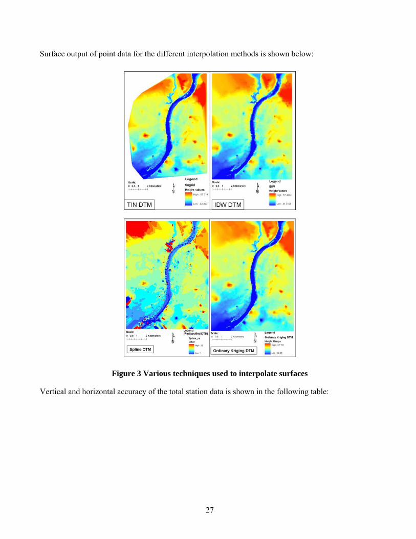
Surface output of point data for the different interpolation methods is shown below:

Figure 3 Various techniques used to interpolate surfaces

Vertical and horizontal accuracy of the total station data is shown in the following table:

28

Table 1 Comparison of horizontal and vertical accuracies of different surfaces obtained by TS

data interpolation techniques

S

No.

Interpolation technique RMSE Horizontal

accuracy

(meters)

Vertical Accuracy

(meters)

1 TIN 0.8541 1.48 1.67

2 Inverse Distance

Weighting

0.7778 1.35 1.52

3 Spline 1.088 1.88 2.13

4 Ordinary Kriging 0.6017 1.04 1.18

5 Simple Kriging 0.7705 1.33 1.51

6 Universal Kriging 0.7677 1.33 1.50

3.1 Generation of Digital Surface model

Digital surface model (DSM) was generated by adding the man made structures like residential,

commercial, institutional and other buildings, roads from (Katuri, A. K., Sharifi, M. A. and van

Westen, C. J. 2006). Same exercise was repeated for the post-SRFDP scenario. These two surface

models were used to simulate the flood viz. both pre and post project scenarios.

Meteorological information

The weather graph of Ahmedabad can be distinctly divided into three seasons, namely, the cold dry

winters, the hot dry summers and the monsoon season. The mercury starts soaring in Ahmedabad from

early spring (March), reaching its peak in the month of May (43.40 Celsius). The temperature remains

high until June, then falls drastically during July and again rises rapidly in the month of October (as

high as 39.40 Celsius). January is the coldest month of the year with mercury dipping down to 4.90

Celsius.

Like most parts of the country, Ahmedabad receives its maximum precipitation from the southwest

monsoons during the months of July and August. As is observed from the graph, the total precipitation

for the year 2000 is 72.71 cm. Out of this 59.0 cm is received in the months of July and August alone.

29

Some pre-monsoon showers bring relief during May and June while rest of the months remains dry

throughout the year.

Correspondingly, the Relative Humidity is also high during the rainy season reaching its peak in the

months of July (98%) and August (90%) respectively.

For the current study, we have just considered the riverine flooding. So the rainfall data has not been

analysed. Discharge data from the year 1979 to 2006 is collected from the Gujarat Water Resources

Development Corporation (GWRDC). This data is analysed and used for the modelling.

4.1 Magnitude-frequency analysis

This was carried out to find out the relation between probability of the occurrence of a certain flood

event, its return period and its magnitude. For this, we used two methods: Gumbel’s method and Log

Pearson type III method.

Gumbel’s method:

Gumbel’s probability was plotted to obtain the return periods using the following equations.

1+=

NRPL …………………………… Equation 1

Where: PL is the Left sided probability (probability of having less values in the series)

N = number of observation

R = Rank

Now return period for each observation is determined using equation 2

LR PPT

−==

111 …………………………… Equation 2

Where T = Return Period

PR = Right sided probability

The plotting positions ‘y’ are determined using the third equation

)lnln( LPy −−= ……………………… Equation 3

30

The return periods obtained from the Gumbel’s plots are shown in Figure 4 below.

Figure 4. Gumbel’s plots for the probability distribution of return periods

In the maximum discharge, we have some smaller outliers at the origin, indicating a possibility of two

trends instead of the one depicted above. Using this frequency analysis the design hydrographs were

obtained for the return periods of 10, 25, and 50 years based on 2006 year flood wave.

4.2 Correction for Outliers

Outliers are the data values which deviate from the general trend of the data. In our case, the lower

outliers are located at the origin. Based on the coefficient of skew, the check for outliers is performed

for structural break. If the skew is higher than + 0.4, the data is tested for the higher outliers. If the

skew is less than -0.4, then a test for lower outliers need to be performed. Similarly, if the skew lies

between +0.4 and -0.4, then test for both outliers is performed. In this case, skew was less then -0.4

(0.039), so the low outliers were detected using the using equation from(Chow, Maidment, DR and

Mays, LW 1988):

ynL sKyy −= ……………………………………..Equation 4

Where: Ly = Low outlier threshold in log units

nK = One-sided 10 % significance level for the normal distribution

ys = Standard deviation of y

31

y = Mean of y

y = Log x (Log of yearly maximum flow rates)

The low outlier threshold obtained was 684 m3/sec. All the values below this were eliminated from

calculation of magnitudes using Gumbel’s method. After removing the outliers the remaining data was

limited to 16 years instead of total 28 years. The new lower outlier adjusted Gumbel’s plots are shown

in Figure 5. The design hydrograph for different return periods after the outlier adjustment are shown in

Figure 6.

Figure 5: Gumbel’s plots for the probability distribution of return periods after adjusting lower

outliers

Gumbel's Method For 10, 25 and 50 year return Periods with outlier adjustments

02000400060008000

1000012000140001600018000

17 18 19 19 20 21 22 22 23 24 25 25 26 27 28

Time (Days)

Flow

Rat

es (c

um/s

ec) 2006 Flood

10 Year Return Period Flood

25 Year Return Period Flood

50 Year Return Period Flood

Figure 6 Gumbel’s Method of flood Magnitude – frequency analysis for 10, 25 and 50 years of

return period after adjusting the lower outliers

32

Log Pearson type III

Here, the variate is first transformed into logarithmic form (base10) and transformed data is then

analysed. According to (Chow et al. 1988), the magnitude xT of a hydrologic event may be represented

as the mean µ plus the departure ∆xT of the variate from the mean.

TT xx ∆+= µ ……………………………….Equation 5

The departure may be taken as equal to the standard deviation σ and a frequency factor KT; that is,

σTT Kx =∆ ……………………Equation 6

The departure ∆xT and the frequency factor KT are functions of the return period and the type of

probability distribution to be used in the analysis. Thus the equation 1 can be expressed as:

σµ TT Kx += …………………………….Equation 7

Or it can be approximated by

sKxx TT += …………………………..Equation 8

When the variable analyzed is y = log x, then the using the equation for applying the statistics for the

logarithms of the data, then the equation 4 becomes

yTT sKyy += ……………………….Equation 9

Once the value of y is obtained, then the frequency factor KT is calculated using the equation

5432232

31)1()6(

31)1( kzkkzkzzkzzKT ++−−−+−+= …..Equation 10

Where: KT = Frequency factor

K = Cs/6

Cs = coefficient of skewness

31

3

)2)(1(

)(

y

n

ii

S snn

yynC

−−

−=

∑=

33

n = Total number of years for data available

yi = y for a particular year

y = Mean of y or Log x

sy = Standard deviation of y

21

1

2)(1

1⎟⎠

⎞⎜⎝

⎛−

−= ∑

=

n

iiy yy

ns ……………………. Equation 11

z = standard normal variate

Finally, the frequency factor KT is calculated using the equation

5432232

31)1()6(

31)1( kzkkzkzzkzzKT ++−−−+−+= ………..Equation 12

Where: KT = Frequency factor

K = Cs/6

The required value of Return Period xT is calculated by taking the antilog of yT using the equation 9.

For detailed information on this method please refer (Chow et al. 1988). Then use the value of KT and

Sy were used in equation 9 and calculated the value of yr. The return period was calculated by taking

the antilog of yr.

The design hydrographs obtained by this method for different return periods of 10, 25, and 50 years

along with year 2006 are presented in the following diagram..

Pearson Type III Distribution For 10, 25 and 50 year return Periods

010002000300040005000600070008000

17 18 19 20 21 22 23 24 25 26 27 28

Time (Days)

Flow

Rat

es

(cum

/sec

) 10 year Return25 Year Return

50 Year Return

2006 Year flood

Figure 7 Log Person Type – III Flood Magnitude – frequency analysis for 10, 25 and 50 years of

return period with year 2006 data

34

4.3 Reliability of predictions

The reliability of both Gumbel’s and Pearson Type III methods was estimated at 90% confidence limits

for 50 year discharge in Sabarmati river based on 28 years data. The maximum flow rates predicted by

Guumbel’s method with and without lower outlier adjustment and the Pearson Type III are shown in

Table 2.

For β = 0.9, α= 0.05 and the required Standard Normal Variate Z has the exceedence probability 0.05.

The upper and lower limits were calculated for testing the reliability of prediction of 50 year return

period and the predicted values of 50 year return period, for both methods were assessed within these

estimated limits. The value for Qmax for 50 year return period at 90% confidence limits by Gunbel’s

and Pearson Type III method must fall within the intervals of 15524 > x > 4573. The value produced

by Gumbel’s method (without outlier adjustment) and Perarson Type III, lies perfectly within the limit,

but the Gumbel’s (with outlier adjustment) predicted the value overshoots the 90% confidence limits.

 

Table 2 Comparison of the flood frequency analysis methods

Return

Period

(Tr)

Gumbel (No

outlier adjustment)

Qmax (m3/s)

Gumbel (with

outlier adjustment)

Qmax (m3/s)

Pearson Type

III Qmax (m3/s)

10 year 960.1436 3480.127 3331.331

25 year 2511.504 8448.343 5461.631

50 year 5097.105 16728.700 7516.807

Although, 90% confidence limits supported both Gumbel’s and Pearson Type III methods but it suffers

a bias introduced by the lower outliers. Due this lower outlier effect the predicted value for 50 year

return period were much lower than that of 2006 year flood event, the maximum in last 28 years

(Figure 6). The results obtained by Gumbel’s method after removing the lower outliers overshoot the

90% confidence limits of the reliability test. The Pearson Type III suffered from no such problems and

was based on entire dataset available for frequency analysis. Thus, Pearson Type III was preferred over

Gumbel’s method for simulating flood modelling for the return periods of 10, 25 and 50 years.

35

Flood hazard assessment

Flood in Ahmedabad city is assessed using the above meteorological data for two different situations.

One is as is situation and the other one is with complete implementation of the ongoing River Front

Development Project. The DSM is conditioned for the new river sections after the implementation of

the project.

The data available after the removal of outliers is only for 16 years. Using this data, flood scenarios for

three return periods were simulated

5.1 SOBEK model

We used SOBEK 1D and 2D models for simulating river flow and overland flow respectively. Both

ends of the river in the city (Sardar Bridge on north and Vasna barrage in south) were considered as

boundary conditions. The flow rates at the Vasna barrage were used to calibrate the model results.

Because of the limitation of the software to handle not more than 100,000 pixels, we have to loose the

resolution of the DSM from 5 meter to 20 meters.

5.2 Surface roughness

Surface roughness was expressed using Manning’s coefficients. Manning’s coefficients were taken from the

National Institute of Hydrology’s report, “Hydrologic Studies for Sabarmati Riverfront Development Project” for

the Ahmedabad Municipal Corporation. Table below show the Manning’s coefficients used in the

simulation.Table 3 Manning’s roughness coefficients adapted for the model.

Land use category Manning’s

value

Natural River section 0.25

Modified River section 0.30

Agricultural land 0.040

Industrial /Commercial 0.032

Open area 0.025

Residential 0.035

36

The schematisation of the network is a crucial step in the simulation. First, the river network in 1D

(centreline of the river) was imported from ArcGIS into the netter in SOBEK environment. For

defining the representing system, river shape, location, river cross-sections, calculation points,

boundary nodes, 2D grid, connection nodes, measurement stations, and hydraulic structure like orifice

etc. were defined. Then, the terrain information was imported to SOBEK in ASCII format. This DEM

plays an important role in modelling flood in SOBEK. As discussed earlier, the pixel resolution,

SOBEK can handle depends on the number of pixels. He computation time in SOBEK goes up

enormously if the number of pixels is higher. Care was taken to restrict the total number of pixels (less

than 100,000 pixels) for efficient functioning of the model. In the 2D schematization history nodes

were placed at selected areas to record detailed time series of water depths and velocities.

Figure 8 SOBEK Schemetisation in 1D2D with details

Figure 9 River sections after implementation of SRFDP

37

In order to assess the impact of flood hazard after the completion of the SRFDP, the digital surface

model was modified to incorporate the new river sections as shown in Error! Reference source not

found.. the cross sections were added at an interval of 200 mt. SOBEK interpolates the surface between

these cross sections.

Output from SOBEK is exported into .asci format. Using various techniques, these input are

converted into ArcGIS environment to visualise and assess the associated risk.

Results of flooding scenarios

After successful simulation of the 2006 event, the calibrated model was applied to both natural and

modified river sections that represented the new river front known as Sabarmati River Front (SRF). The

flood simulation results for both Pre and Post SRFDP situation for the return periods of 10, 25 and 50

year, are presented in next sub-section.

6.1 Flood depth maps for 10, 25 and 50 year return period

The flood depth maps for a 10 year return period for Pre and Post SRFDP are presented in figure 4-6.

It can be seen that after SRFDP implementation there is no chance of occurrence of flood once in 10

years. On the other hand, the natural state of the river still produces some flood inundating an area of

1.6 meter square. Although there will be flood, but the only people who will be affected are those

staying near the river bank. This includes a large number of slum dwellers. For the floods that have a

chance of occurrence once in 25 years, the SRFDP again proves to be efficient in restricting the flood

from spreading to larger areas as compared to that of the natural river section. This is evident from

Figure 11, that the there is a 75% reduction of inundated areas with the SRFDP in place. But with a

severe flood of high magnitude, having a change of occurrence once in 50 years, SRFDP no longer

proves effective and the flood inundates almost equal areas - Figure 12. For actual quantification of

flood hazard please refer Figure 13. The visual examination of all the flood depth maps provides a clear

indication of the potentials of SRFDP towards mitigation of this disaster.

38

Figure 10 Flood inundation Depths maps for 10 year return period

Figure 11 Flood inundation Depths maps for 25 year return period

39

Figure 12 Flood inundation Depths maps for 50 year return period

Flood hazard assessment is conducted in two different ways. First, the hazard is presented in the form

of flood spatial extents. This is done with respect to different return period flood and the increase or

decreased is quantified in terms of inundated area.

The second assessment expresses the hazard in terms of severity, based on inundation depths and flow

velocity. In the last section the suitability of SRFDP in combating the flood situation is compared in Pre

and Post SRFDP states of Sabarmati River.

6.2 Flood hazard – spatial extents

The visual assessments in the previous chapter demand the importance of quantification of flood

hazards and a comparison of the two situations. In this section, the flood hazard is quantified and

compared in terms of its spatial context. The inundation depth maps produced by model were colour

coded and overlaid. The river was kept separate to assess the correct measurements. The area obtained

from all the flood extents maps were presented in table 5-1, and the Pre- and Post SRFDP situations

were compared.

 

40

Table 4 Comparison of the inundated areas for Pre (Natural) and Post SRFDP state

Return Periods

(years)

Pre – SRFDP

inundated area

(km2)

Post – SRFDP

inundated area

(km2)

Change in

inundated area

(km2)

10 1.60 0.00 1.60

25 7.22 3.14 4.08

50 12.11 12.90 -0.79

The figure indicating the change in area column in

Table 4 shows that Post SRFDP flood are much smaller in spatial extents in comparison to the natural

section of the river. The only exception to the decrease in extents is a flood of very high magnitude

with a probability of occurrence of one in 50 years. While simulating the results, it was evident that the

river overtops the banks at a very late stage. However the flood occurs at northern end of SRF where

the river width is much higher that the constricted conditions.

The study shows that the intervention in the river course by this project does alter the flood extent in

the lower return period events. In the higher return period events, i.e. 50yrs event, the project is

negatively impacting the flood extent. With the change in the rainfall pattern (Das, Saurabh, Shukla,

Ashish K. and Maitra, Animesh 2010) there is a need for more detailed analyses to be carried out

before finalising a project which changes the river course.

41

Figure 13 Comparison of Pre and Post SRFDP flood hazard extents

42

References:

Burrough, P. (1986). "Principles of geographical information systems for land resources assessment."

Geocarto International 1(3): 54-54.

Census (2001). District Census Handbook.

CEPTUniversity (2007). CDS, City Development Plan. Ahmedabad, India.

Chow, D. Maidment, et al. (1988). Applied hydrology, McGraw-Hill, New York.

Das, S., A. K. Shukla, et al. (2010). "Investigation of vertical profile of rain microstructure at

Ahmedabad in Indian tropical region." Advances in Space Research 45(10): 1235-1243.

Gao, J. (1997). "Resolution and accuracy of terrain representation by grid DEMs at a micro-scale."

International Journal of Geographical Information Science 11(2): 199-212.

Gopalakrishnan, M. (2006). "Challenges of Water for Food, People and Environment–." Water and

agriculture: sustainability, markets and policies: 221.

Katuri, A. K., M. A. Sharifi, et al. (2006). "Urban mapping and land use characterisation for risk

assessment." Presented at the 2nd international symposium on Geo-Information for disaster

management Gi4DM : remote sensing and GIS techniques for monitoring and prediction of

disasters, 25-26 September, 2006, Goa, India. 7 p.

Maune, D. (2007). Digital elevation model technologies and applications: The DEM users manual,

American Society for Photogrammetry and Remote Sensing.

NIH, N. I. o. H. (2007). "Hydrologic Studies for Sabarmati Riverfront Development Project."

Retrieved 20th September, 2010, from www.egovamc.com/sabarmati/NIH_report.pdf.

Wilson, J. P. e. and J. e. Gallant (2000). Terrain analysis : principles and applications. New York etc.,

Wiley & Sons.

Wood, J. (1994). "Visualizing contour interpolation accuracy in digital elevation models." Visualisation

in geographical information systems: 168-180.

43

STUDY OF DRAINAGE PATTERNS AS OBSERVED ON REMOTE SENSING

IMAGES OVER JHARIA- RANIGANJ COAL FIELD OF EASTERN

INDIA

V. K. Srivastava

Dept of Applied Geophysics, Indian School of Mines, Dhanabd 826004

E mail: ism_vinay@yahoo.co.in

Study of drainage pattern as observed on remote sensing images has been carried out covering

Jharia -Raniganj coal fields of Gondawna terrain of Damodar Valley of eastern India ( see fig 1)

from the point of view of surface water resources management, and is briefly presented here.

A. The Jharia coal field which lies in Dhanabd Dt of Jharkahnd and is the only source of prime

cocking coal of the country shows coarse subdendiritic pattern with general flow direction to south and

south east. on a gentle rolling topographic surface ( see fig 2 and 4). The streams are effluents in nature

and show characteristics of a hilly river ie they swell with sort spell of rain and drain quickly as the

rain stop. The river Damodar which is the trunk river is of perennial in nature and flows

approximately in a faulted southern margin of the coal field. The important tributaries of this trunk

river are Jamunia , Katri , Khudia , Ekra and Kari Jhors which are seasonal in nature and are flowing

in south and south easterly directions. .Drainage dissection has been also observed along Jamunia and

Katri rivers. These drainage lines cut across the whole sedimentary section and the interfluve region

in between shows very little variations in relief. Drainage density varies from 0.5 to 1.5 over with

basin of sizes ranging from 8 to 170 sq km .and of average stream lengths from 10 to 120 km. The

valley sections of these channels are flat and shallow and water flow in these streams are sluggish

and slow reflecting “old age” streams in matured eroded surface of gentle slope( 1 to 3 degree). The

commonly observed zig- zag drainage lines of the tributaries suggest that the flow lines are

controlled by criss cross joints , fractures and cross faults of sedimentary formations in the basin

and of post Gondwana age.

.

B. The Raniganj Coal field is approximately SSE above described Jharia coal field and lies in the

Burdwan district of West Bengal9 see ffgi 4 and 5). The basin is drained by three perennial rivers viz,;

Damodar , Barakar and Ajay having and the two group of tributaries are observed one joining

44

Damodar flowing mostly over Gondwana terrain and other joining Ajay river flowing mostly over

archaen terrain . Structure of the basin is like half graben with mild slope of 3 to 5 degree.

The Damodar river enters the coal field near Somaliya village ( 86 40 E, 23 40 N ) and flows in a

south - south easterly direction forming approximately the southern faulted margin of this coal field

and finally leaves the region to the north of Jalanpur village ( 87 E 23 45 N). The river Ajay enters the

region from Chitranjan and partly form the northern depositional margin of this basin. The Barakar

river after entering the area near Sijua settlement ie north of Karma tanr ( 86 12 E 23 53 N) joins the

main river Damodar to the west of Dishergarh..

Besides these 3-perennial rivers, the region is drained by 15 nalas and jors and the prominent one

are Barajouri ,Choupahri, Harial jhor , Khol , Machkanda ,Nonia, Paunta and Sigaran nala with

stream length varying from 10 to 20 km and having basin size ranging from 15 to 120 Sq km and

drainage density from 0.5 to 2.0. The general drainage pattern in the region is dendiritic to sub

dendiritic flowing over a eroded plain of gentle slope( 5 to 8 degree) . These seasonal water channels

remain dry or contain little water during most of the months of the year except during the rainy

season. Drainage section is again shallow and flat which is filled with sediments generated by sheet

erosion of gently sloping surrounding terrain. It is observed that the drainage lines within the basin are

controlled by criss cross joints and fractures and cross faults within sedimentary formations and also

at places they are controlled by the out cropping iron stone shale and dolerite dykes.

45

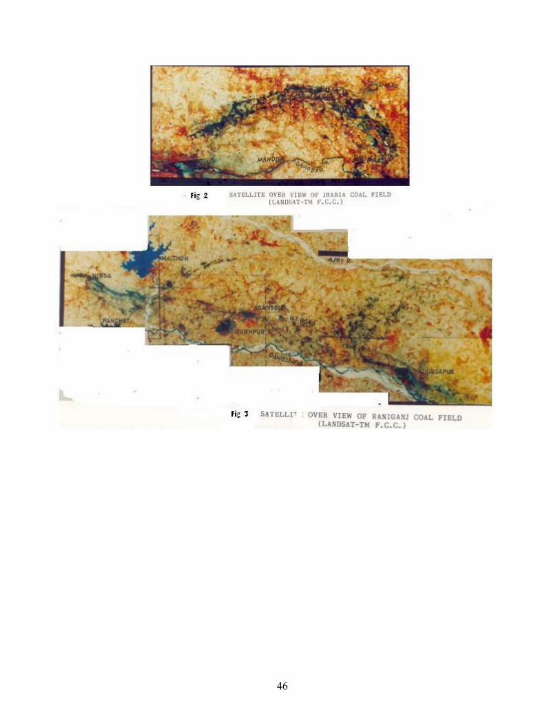
46

47

48

Reference

Srivastava V K,1997, “ Study of Drainage Pattern of Jharia Coal Field ( Bihar ) , India through Remote

Sensing Technology “ Journ. of Ind. Soc of Remote Sensing , Vol 25, No 1, pp42-46

Srivastava V K and Mitra D ,1995, “ Study of Drainage Pattern of Raniganj Coal field (Burdwan Dt ) as

observed on Landsat TM /IRS LISS II Imagery “ , Jourl of Ind Soc of Remote Sensing , Vol 23 , No 4 pp

225-235.

Srivastava V K ,1991, “ Remote Sensing Applications in Monitoring Environmental Impacts of Mining in

Jharia- Raniganj Coal Filed” Final Report submitted to Ministry of Environment and Forest under PC-

NNRMS , New Delhi ,pp 1- 161.

Section II

49

SOILS AND THEIR MINERAL FORMATION AS TOOLS IN PROVENANCE, CLIMATE CHANGE AND GEOMORPHOLOGICAL RESEARCH

D.K. Pal

Global Theme-Agro-Ecosystems, ICRISAT, Patancheru, Hyderabad, Andhra Pradesh

Email:paldilip2001@yahoo.com

Abstract

Secondary minerals at a less advanced stage of weathering may adjust to subsequent environmental changes.

Therefore, they may lose their interpretative value. However, pedogenic minerals like di- and trioctahedral

smectite, smectite-kaolin interstratified mineral, hydroxy inter-layered vermiculite and smectite and pedogenic

calcium carbonate have been found to be useful as paleo-environmental indicators because these pedogenic

minerals in three major soil types (red, black and alluvial soils) and drill cores of the Ganga Plains of semi-arid

parts of India, could be preserved unchanged amidst climate change from humid to semi-arid climate. Studies

on the genesis of these pedogenic minerals so far conducted at the NBSS&LUP (ICAR), Nagpur, Geosciences

Laboratory, Civil Engineering Department, IIT, Kanpur and Department of Geology, Delhi University, Delhi,

India for the last two and a half decades have helped the pedologists and geoscientists not only to unravel the

past geomorphic processes in the formation of spatially associated red (Alfisols) and black (Vertisols) soils of the

Peninsular India and the existence of Vertisols amidst micaceous Indo-Gangetic alluvial Plain, but also to infer

the provenance and climate change in the Himalayan Foreland and polygenesis in the major soil types of the

Indian subcontinent.

The review on the research results obtained by these national institutes indicate that the X-ray diffraction

analysis of the soil clay fractions and also the micromorphological thin section studies specially of carbonate

minerals and plasmic fabrics have become formidable analytical tools in provenance and climate change

research.

Keywords: Climate change, mineral formations, soil and earth science research

50

IMPACT AND HAZARDS OF FLOODING IN MUMBAI

M Chandradas

Geological Survey of India, Central Region, Nagpur chandradasm@yahoo.com

Abstract

Mumbai metropolitan region and Suburban areas received heavy rains on 26th and 27th July

2005which was struck with a heavy storm that resulted in the flooding of many parts of the Mumbai

City and Suburbs. The entire city had to face multiple hardships, due to disruption of power supply,

stoppage of road and rail communication network and other essential commodities. The above disaster

was an eye opener to all major cities in India to study the effects of urban conditions on rainfall–runoff

relationships. Changes in the physical characteristics of urban areas due to the developmental works,

involve physical and topographical changes, thus altering the natural processes in the area. In depth

basin analysis, study of the catchment area is necessary to understand the process of inundation and

flooding. The soil type, the vegetative cover, topographical features of the land surface and the physical

structure in the catchment play a key role in influencing the runoff process. Urban areas tend to reduce

the natural vegetative cover due to developmental structures such as roads, pavements, buildings

(residential and non-residential), paved parking lots and sidewalks, driveways that collectively increase

the impervious surfaces in the catchments. Areas are reclaimed by dumping constructional

waste/weathered Deccan trap material over the mudflat and leveled and compressed by rollers thereby

reducing the ground porosity, clogging the natural drainage and increasing the surface runoff, which

other wise would have been natural soak pits during precipitation. Major causes for flooding in

Mumbai are due to the very low gradient, the mudflat areas have a gradient of less than 2o and are

affected due to tidal changes in sea .Also, the monsoon pattern has changed. But the drainage

system has only not lived up to its capacity. For Water Management, topographic map play a very

important role. These Maps gives us the basic information regarding ground slopes, which enables us to

establish floodplain zones and delineate the areas subject to flooding. The most ignored system in

Mumbai is its natural drainage, its rivers and rivulets. Of these, river Mithi is the most important,

drainage of Suburban Mumbai. Others rivers have almost disappeared; the Mithi still flows as a

stinking choked nullah The River originates in the Sanjay Gandhi National Park — thus, it is rain-

fed. It flows to the Tulsi Lake, and then to Vihar and Powai lakes. From Powai Lake it starts an

51

approximately 15 km journey that ends in the Arabian Sea at Mahim creek. It is pathetic that many

of the Mumbai citizens and even the civic administration are not aware of the presence of a river

in heart of Mumbai.

The field observations indicate that all the rivers in Mumbai are suffering from the following

five assaults:

• Open, dangling cable and pipe crossings on the sides of the bridges and culverts,

• Debris dumping (from construction activities as well as industrial wastes) on banks and into rivers,

• Sedimentation in river beds and dumping of urban solid wastes into rivers coupled with nil to

inadequate annual desilting efforts,

• Ingress encroachments from the banks (building, industries, and slums); and modification of river

courses and local diversion of streams.

Recommendations towards maintaining ecological balance, we have to first restore the existing

degraded rivers and river-banks to initiate recovery of the urban ecosystem, provide river flushing

system to initiate rejuvenation of river channels. Restore the Mangrove-Ecosystem and rejuvenate the

coastal zones and construct detention basins and infiltration zones for flood control and provide broad

roads near toll tax areas for people to escape in case of disasters and calamities.

Remove encroachments and facilitate flow in all the Creek System and strictly adhere to the

Development Plan. Implementation of India’s environmental policy in a proactive manner and ensure

compliance of environmental regulations by the Municipal Corporation.

Reference

1-D Mathematical Model and Desk Studies for mitigating floods of MIthi River of Mumbai, Technical

Report No. 4297, CWPRS, Pune, January 2006.

Seismic hazard Microzonation of Mumbai Urban Agglomeration Unpublished report GSI 2009

Monograph on flood hazard Environmental information system India

Gupta, Kapil, “Urban Flooding: Vulnerability, Preparedness and Mitigation – 944 mm Mumbai 26/07/2005

event”, Presentation, International Centre for Excellence in Water Resources Management,

Adelaide, 29 May 2006.

52

PROCESS AND FORMS OF MOUNTAINOUS TROPICAL RIVER SYSTEMS -

EXAMPLE FROM KERALA STATE, SOUTH INDIA

S. Manjua and S. Anirudhanb

aGeological Survey of India, Central Region, Nagpur bDept. of Geology, University of Kerala, Kariavattom

manjusudevan@gmail.com

Abstract

The south western part of Indian peninsula is unique with respect to climate physiographic and

drainage conditions. Presence of Western Ghats running roughly parallel to the western shoreline of

India plays a significant role in determining the uniqueness of this morphogenetic region. The entire

state of Kerala fall in this typical morphogenetic region is characterized by number of short and swift

west flowing rivers and tributary system. Out of the 44 rivers originating from the Western Ghats 41

flows in the west direction draining the Kerala state which has a total area of 38,590 km2. Maximum

transect width of this country is only 124 km which clearly vouch for the short run of even the largest

river of this region. The entire region experience a typical tropical climate which comes exactly within

the Tropical Am and Tropical Aw regions of Koppen (1939). By considering the classification of

Indian rivers according to Gupta (1984) only five rivers can be grouped under medium river (catchment

area between 2000-20000 km2) and the rest can be classified as minor rivers (i.e., catchment area <

2000 km2). Geologically the area is occupied by Precambrian crystalline rocks, viz., Khondalite and

charnockite. This region is conspicuous by absence of any major sedimentary basin except for a fringe

of Tertiary formation along the coastal margin. The regional structural grain of Precambrian rocks as

evident from the satellite imagery has NW-SE or NNW-SSE direction.

Because of the archetypal climatic, geologic and physiographic milieu, the region enjoys a

unique geomorphic process. The dominant fluvial process operates in this region with its full sequence

right from weathering through all progression of mass wasting. The ubiquitous laterite, a residual

product of chemical weathering of tropical climate gives sufficient stability to the slopes of this region.

However, partly weathered portion is susceptible for slide or slump in the highland and steep slopes.

Channel forms of almost all rivers are more or less uniform for minor and for medium rivers. The

most notable channel form features from upstream to downstream direction of majority of mountainous

53

rivers of Kerala are bedrock channel floors with rapids and falls, boulder - pebble bedded channel

floor with unstable banks, sandy bar- pool sequence with more or less stable banks (laterite?) and wide

and deeper channel with unstable banks (floodplain). The tectonic and climatic implications of the

varied channel form features are explored in this study.

Key words: Tropical Rivers, process and forms, morphogenetic landforms

54

QUATERNARY GEOLOGY OF CENTRAL INDIA

M P. Tiwari

Nagpur 

Abstract

In central India, Quaternary sediments occur as thick deposits of deep, structural riparian basins

and thin deposits of shallow river valleys. Quaternary sequences from Lower Pleistocene to Holocene

are seen in structural basins, whereas shallow river valley deposits show upper Pleistocene to Holocene

sequence. Formal Quaternary lithostratigraphic formations have been described only in the Narmada

valley and it is proposed that nomenclature and succession of the Narmada valley may be adopted in

other river valleys of the central India. Quaternary stratigraphic succession, proposed for Central India

comprises; 1. Ramnagar formation, 2. Hirdepur formation, 3. Baneta formation, 4, Surajkund

formation, 5. Dhansi formation and 6. Pilikarar formation. Each formation has characteristic

soiI/palaeosol at its top. Soils on the older formations, are ferruginous while soils on the younger

formations are calcic. Tephra beds are seen at two levels; as insitu tephra below the brown soil

developed on the Baneta Formation and as reworked tephra associated with coarse basal units of the

Hirdepur Formation. Geochemistry and fission track dates relate the tephra beds of the Narmada, Son,

Purna and Kukdi valleys with the Youngest Toba Tephra of 75 ka. Radiocarbon dates suggests that: 1.

The Ramnagar formation is younger than 4.5 ka and 2. Hirdepur formation comprises sediments

deposited during 25 to 13 ka Last glacial maximum). The Baneta formation with insitu tephra

represents the early last glacial (Early Upper Pleistocene). Hirdepur and Baneta formations comprise

mammalian fossils of Upper Pleistocene affinity and the underlying Surajkund formation comprises

fossils of Middle Pleistocene affinity. The fossil of Homo erectus was recovered from the Surajkund

formation. The boundary between the Surajkund formation and the underlying Dhansi formation also

marks the boundary between Brunhes Normal magnetic polarity epoch and Matuyama reverse polarity

epoch.

 

  55

LATE QUATERNARY FLUVIAL HISTORY OF THE UPPER BRAHMAPUTRA VALLEY, NORTHEASTERN INDIA

By

N.R.Ramesh

Geological Survey of India, Bangalore

Email: n.ramesh@gsi.gov.in, geo_nittur@yahoo.co.in,

Abstract

Systematic geological mapping and allied researches in the Brahmaputra valley in parts

of Assam and adjoining Arunachal Pradesh have provided evidences of Late Quaternary changes

in the river regimes, possibly in response to global climatic changes and mild neotectonic

movements. Recently, evidences of river metamorphosis, unilateral migration, severe bank

erosion and flood hazards are also reported from parts of Upper Assam and foothill plains of

Arunachal Pradesh. Building up of morphostratigraphic sequence in the alluvial plains combined

with radiocarbon dates has enabled the identification of major episodes of erosion and deposition

in the region. The surficial study of Quaternary formations in and around the Bengal Basin has

broadly indicated the presence of four-tier sequence of Upper Pleistocene to modern sediments.

A comparative study of the data from the Brahmaputra valley and adjacent isolated narrow

basins brings out two distinct ages of these sediments, namely the Pleistocene and Holocene. The

form and content of the terrace deposits and misfit river reveal that the rivers have progressively

shrunk in size since the late Pleistocene time. Supporting evidences from the Indo-Gangetic

valley, Deccan region and Arabian Sea demonstrate that the successive phases of aggradations

and incision are possibly linked to late Quaternary climatic changes and local tectonic

movements.