WP/15/256

If the Fed Acts, How Do You React? The Liftoff Effect on Capital Flows

Swarnali Ahmed

IMF Working Papers describe research in progress by the author(s) and are published

to elicit comments and to encourage debate. The views expressed in IMF Working

Papers are those of the author(s) and do not necessarily represent the views of the IMF, its

Executive Board, or IMF management.

© 2015 International Monetary Fund WP/15/256

IMF Working Paper

Strategy, Policy and Review Department

If the Fed Acts, How do You React? The Liftoff Effect on Capital Flows

Prepared by Swarnali Ahmed

Authorized for distribution by Martin Kaufman

December 2015

Abstract

After more than six years of ultra-low interest rates, a Fed liftoff (rate hike) is just a matter

of time. This paper goes back to history to understand the spillover effect – or what is

termed in the paper as the ‘liftoff’ effect – of the previous five Fed liftoffs on capital

flows. Using a dynamic panel framework covering 48 countries (27 advanced economies,

21 emerging markets) over the period 1982-2006, the paper shows that the liftoff effect on

capital flows (total private, portfolio) is significantly higher for emerging market

economies (EM) than advanced market economies (AM). EM capital flows are hit

indiscriminately one quarter before liftoff, suggesting that markets usually price in the

liftoff before the actual event. Over time, there is a bit more variation among EM as policy

responses/framework can to some extent dampen market reactions. The findings are

similar to the unfolding of events during the taper tantrum episode indicating that, even

though current circumstances are very different, history could still provide a good

guidance.

JEL Classification Numbers: F32, E52

Keywords: Fed liftoffs, policy responses, policy framework, capital flows, emerging market

economies.

Author’s E-Mail Address: sahmed@imf.org

IMF Working Papers describe research in progress by the author(s) and are published to

elicit comments and to encourage debate. The views expressed in IMF Working Papers are

those of the author(s) and do not necessarily represent the views of the IMF, its Executive Board,

or IMF management.

3

Contents Abstract ..................................................................................................................................... 2

I. INTRODUCTION ................................................................................................................. 4

II. THE LIFTOFF EFFECT OF THE U.S. RATE ................................................................... 6

A. Empirical Strategy............................................................................................................ 6

Step 1: The Generic Model for Capital Flows .................................................................. 7

Step 2: The Saturated Model Introducing Liftoff Effects ................................................. 8

Step 3: The Restricted Model from the Saturated Model ............................................... 10

Robustness Checks.......................................................................................................... 10

B. Results ............................................................................................................................ 11

Model Results ................................................................................................................. 11

Using Model Results to Get a Sense of Magnitude ........................................................ 12

C. Why a Liftoff Effect Prior to Liftoff? ............................................................................ 13

III. THE LIFTOFF EFFECT OF DOMESTIC POLICIES .................................................... 15

A. The Policies .................................................................................................................... 15

B. Empirical Strategy .......................................................................................................... 18

C. Results ............................................................................................................................ 19

D. Can Policies Mitigate the Negative Liftoff Effect of the U.S. Rate? ............................. 21

The Estimated Extra Impact on Capital Flows during Liftoff Episodes due to One

Standard Deviation Shock in Each Variable ................................................................... 22

The Estimated Extra Impact during Liftoff Episodes using Average Values of Each

Variable ........................................................................................................................... 23

IV. CONCLUDING THOUGHTS ......................................................................................... 24

V. REFERENCES................................................................................................................... 26

VI. FIGURES .......................................................................................................................... 28

VII. TABLES .......................................................................................................................... 34

VIII. APPENDIX .................................................................................................................... 38

4

I. INTRODUCTION1

After more than six years of ultra-low U.S. rates, a liftoff (rate hike) is now just a

matter of time. Though there may be surprises, the Fed has already communicated

significantly about this issue. Yet, the imminent Fed liftoff is causing a lot of anxiety about

the ripple effects on emerging market economies (EM). What makes the anxiety worse is the

continued decline in EM growth prospects. And, the memory of the 2013 taper tantrum – if a

mere announcement could cause such financial shock waves in the EM world, what havoc

would the actual event cause?

This paper goes back to history to understand the spillover effect – or what is termed

in the paper as the ‘liftoff’ effect – of the previous five Fed liftoffs on capital flows. Defining

a liftoff as the first hike in the U.S. policy rate that would be the start of a hiking cycle after a

period of declining or constant policy rate, the paper gauges the extra sensitivity of capital

flows to the U.S. rates during such episodes. The paper then explores what domestic policies

can do during liftoff episodes. Is there room for preemptive measures? Is there any particular

country characteristic or policy framework that makes countries more susceptible to liftoffs?

The paper attempts to answer these questions.

One might argue that this time is different. It is unconventional monetary policies - an

unknown territory. The economic conditions and the financial linkages are also very different

and have evolved over time. What good is history? At the very least, history can provide a

benchmark, a reference point to understand how ‘different’ things are now. The findings

suggest that history can actually be more useful than that. The key conclusions of the paper

are similar to the unfolding of events during the taper tantrum episode indicating that, even

though current circumstances are very different, history could still provide a good guidance

of direction.

Using a dynamic panel framework covering 48 countries over the period 1982-2006,

the paper shows that the liftoff effect on capital flows (total private, portfolio) is significantly

1 I am thankful to Badi Baltagi, Varapat Chensavasdijai, Cristina Constantinescu, Karl Habermeier, Saiful

Hannan, Martin Kaufman, Jeta Menkulasi, Papa N’Diaye, Pau Rabanal, Tahsin Saadi Sedik, Hélène Poirson

Ward, Sophia Zhang, and seminar participants at IMF for their helpful comments and suggestions. All

remaining errors are mine.

5

higher for EM than advanced market economies (AM). EM capital flows are hit

indiscriminately one quarter before liftoff, suggesting that markets usually price in the liftoff

before the actual event. Before liftoff, policy cannot do much to prevent the liftoff effect. In

particular, there is no evidence that countries with more open capital accounts are hit more.

However, over time, there is a bit more variation among EM as country specific policy

responses/framework can to some extent dampen market reactions. In particular, maintaining

monetary policy independence and improving near-term budget deficit seem to mitigate

negative market reactions post liftoff or during liftoff. Also, countries with open capital

account seem to recover quickly over time.

The analysis in this paper contributes to the empirical research on the determinants of

capital flows. The paper broadly relates to three strands of work in this particular field. The

first body of work focuses on the extreme capital flow episodes – sudden stops and surges –

to understand the key determinants of capital flows (Calvo, 1998; Ghosh, Qureshi, Kim and

Zalduendo (2012); Forbes and Warnock, 2012). The empirical specification is consistent

with the basic tenets of portfolio theory in which expected returns, risk, and risk preferences

matter (Ahmed and Zlate, 2014). The determinants are usually divided into external ‘push’

factors – external conditions that attract investors to increase exposure in a particular country

– and domestic ‘pull’ factors – domestic country characteristics that affect risks and returns

to investors. Recent studies have also emphasized the importance of distinguishing between

gross and net flows (Ghosh, Qureshi, Kim and Zalduendo, 2012; Forbes and Warnock, 2012;

Broner, Didier, Erce and Schmukler, 2013). The second strand of literature focuses on the

entire sample, rather than extreme capital flows movements (Ahmed and Zlate, 2014; IMF

2011a; IMF 2011b), with the idea that it is difficult to identify how the longer-term

determinants of capital flows may have changed over time when considering only surges and

stops (Ahmed and Zlate, 2014). More recently, this body of work has also explored the

impact of unconventional monetary policies (Ahmed and Zlate, 2014) and low risk/low

global rate episodes (IMF 2011a). The third body of work focuses on the spillover effect of

monetary policy shocks (Chen, Mancini-Griffoli and Sahay, 2014). The focus is not

restricted to capital flows but on a wide arrange of asset classes. Chen, Mancini-Griffoli and

Sahay (2014) give a good summary of literature in this particular field.

6

The contribution of this paper is that, to my knowledge, this is the first attempt to

look specifically at liftoff episodes to determine the extra sensitivity of capital flows

movements during such times. At the current juncture, this is an extremely policy relevant

question as the Fed is on the brink of hiking after a prolonged period of ultra-low interest

rates. The continued decline of EM growth prospects will make it difficult to disentangle the

liftoff effect from the negative growth effect on capital flows. Looking at previous liftoff

episodes will be useful in making the distinction. The prevailing body of work, while

extremely useful in understanding the determinants of capital flows, may not completely be

comparable to the current situation. This paper builds on the existing literature to make a

more tailor made prescription for the challenges faced by EM in the current global

environment.

The rest of the paper is organized as follows. Section II measures the liftoff effect of

the U.S. rate – the negative impact on capital flows due to the Fed rate hike. Section III looks

at the liftoff effect of policy responses/framework, and discusses which policy responses and

policy frameworks dampen the negative liftoff effect of the U.S. rate. The relative liftoff

impact of the U.S. rate and the policy responses/framework are also discussed. Both the

sections (II and III) identify the timing when the liftoff effects kick in for the U.S. rate and

policy responses/framework. Section IV concludes.

II. THE LIFTOFF EFFECT OF THE U.S. RATE

A. Empirical Strategy

The net capital inflows to emerging and advanced market economies are modeled

using a dynamic panel framework comprising 48 countries (27 AM, 21 EM) over the period

1982Q1-2006Q4. Since the focus is to capture the liftoff effect, quarterly data is used. Higher

frequency data would have been better for such an exercise. However, due to data

constraints, particularly the unavailability of higher frequency data for earlier years in EM,

quarterly data is used instead. The countries and data sources are given in Appendix. All the

results in the paper (and the robustness tests) use robust standard errors (White cross-section

covariance method). Where needed, Breusch-Godfrey tests are also performed to check for

serial correlation.

7

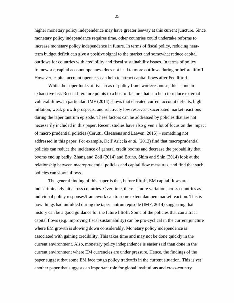
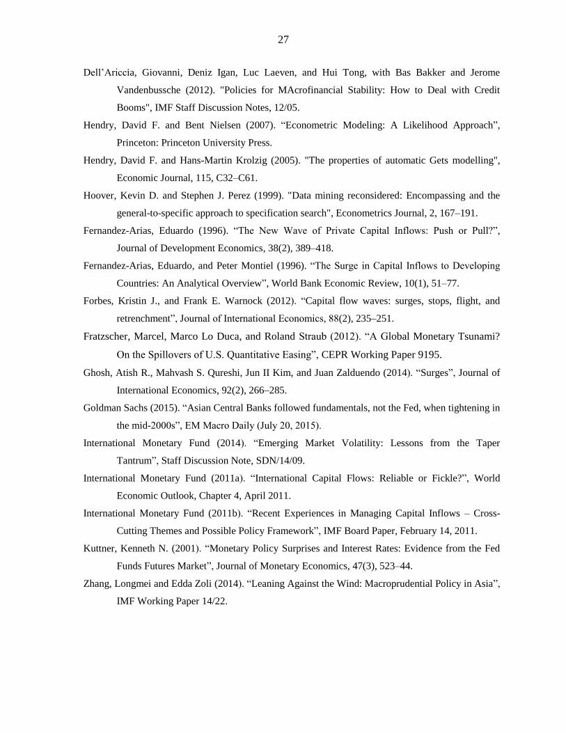
The empirical strategy can be summarized in three steps (figure 1). In the first step, a

general empirical model is built that explains capital flows using the variables (push/pull

factors) that literature has deemed to be important determinants. In the second step, the

“liftoff” effect is captured using an augmented model which includes interactive terms of

liftoff time dummies (explained in detail below) with the U.S. interest rate. This can be

regarded as the saturated model. In the third and final step, the saturated model is reduced by

deleting (after appropriate tests) the interactive terms that are not significant. This sub-

section discusses these three steps in detail and then lists the robustness tests performed.

Step 1: The Generic Model for Capital Flows

Following literature, the determinants of capital flows are grouped into “push” and

“pull” factors (Chuhan, Claessens and Mamingi, 1993; Fernandez-Arias, 1996; Fernandez-

Arias and Montiel, 1996; Ghosh, Qureshi, Kim and Zalduendo, 2012; Forbes and Warnock,

2012; Ahmed and Zlate, 2014). Push factors reflect external conditions that attract investors

to increase exposure in a particular country. Pull factors are recipient country characteristics

that affect risks and returns to investors, and is influenced by local macroeconomic

fundamentals.

Specifically, the starting point is a general empirical model that is often used to

analyze the determinants of capital flows:

( 1 )

The left hand-side, , represents the ratio of net inflows – either total2 or portfolio

only – to country i during time period t, as a fraction of the country’s nominal GDP. The

flows as a share of GDP are modeled as a function of fixed effects ( =1 if an observation

pertains to country i, 0 otherwise), a vector of variables representing external conditions or

2 Unless stated otherwise, total represents total private flows.

8

push factors, a vector of variables representing domestic or pull factors, and s lagged

dependent variables where the length of s is regression specific3.

The external factors include the U.S. interest rate, the U.S. consumer prices (year-

over-year growth), U.S. GDP Growth (year-over-year growth), an index for risk aversion,

and commodity price index (year-over-year growth). For risk aversion or a measure of global

market uncertainty, following an approach similar to Ghosh, Qureshi, Kim and Zalduendo

(2012), the volatility of S&P 500 index returns4 is used rather than the more commonly used

VIX index because the latter is available from 1990 onwards. However, VIX is also used to

perform robustness checks. The domestic pull factors include domestic interest rates,

consumer prices (year-over-year growth), real effective exchange rate (year-over-year

growth), and GDP growth (year-over-year growth). Data sources and list of countries are

given in Appendix.

Presented as such, the model can be regarded as the unconstrained version (Ghosh,

Qureshi, Kim and Zalduendo, 2012). The constrained model would have included real rate

differentials (between the U.S. and the recipient country) and the corresponding GDP growth

differentials instead of the individual components presented in the unconstrained model.

Step 2: The Saturated Model Introducing Liftoff Effects

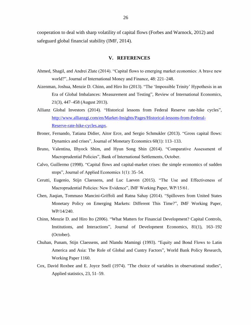
For the purpose of this paper, liftoff is the first increase in the U.S. interest rate which

would eventually be the start of a hiking cycle after a period of declining or constant policy

rate. A liftoff can be regarded as the turning point in the US monetary policy, where interest

rates start to increase after a decline. The “liftoff” effect is defined as the extra sensitivity of

variables during such liftoff episodes. It can be thus regarded as the spillover effect of the

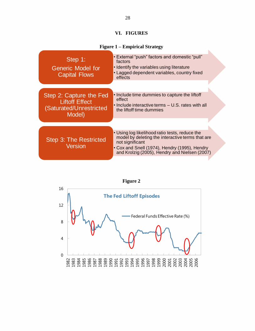
Fed liftoff. Using this definition, five liftoff episodes are identified in the period 1982-2006

(figure 2): March 1983, January 1987, February 1994, June 1999, and June 2004. Since

capital flows data is available on a quarterly basis, the analysis needs to be done using

3 For few regressions, autoregressive errors, AR(), are used instead of lagged dependent variables. The number

of lagged dependent variables or autoregressive terms is quoted in the results.

4 S&P index volatility is the quarterly average of twelve-month rolling standard deviation of S&P index annual

returns.

9

quarterly frequency. The “liftoff quarters” are: Q1 1983, Q1 1987, Q1 1994, Q2 1999, and

Q2 2004. Using this information, five time dummy variables are constructed:

Two quarters before liftoff = 1 and =0 otherwise.

One quarter before liftoff = 1 and =0 otherwise.

Liftoff quarter = 1 and =0 otherwise.

One quarter post liftoff = 1 and =0 otherwise.

Two quarters post liftoff = 1 and =0 otherwise.

The presence of five time dummies is useful to extract a comprehensive picture of

how capital flows react to variables before, during, and post-liftoffs. The liftoff effect may

not necessarily come into play during the liftoff quarter. If the liftoff effect is already priced

in, the spillover effect on capital flows will occur before the actual event. The time dummies

thus help to identify when exactly the liftoff effect kicks in.

The strategy is to interact the time dummies with relevant variables to capture the

liftoff effect and also get a sense of when the liftoff effect kicks in. The liftoff effect of a

particular variable is thus the coefficient of the interactive term comprising the time dummy

and the variable. The dummy variable in the interactive term helps to identify if the liftoff

effect occurs before, during and/or after liftoff. For the first part of the paper, the time

dummies are interacted with the U.S. interest rate to measure the liftoff effect of the U.S.

interest rate. In the second part, the time dummies are interacted with the variables

representing policy responses/framework to measure the liftoff effect of policy framework or

policy responses.

In terms of algebraic formulation, one can easily move from the generic model in

equation 1, to the saturated model:

( 2

10

where are the five dummy variables with j=-2,-1,0,+1,+2 representing two quarters before

liftoff, one quarter before liftoff, liftoff quarter, one quarter after liftoff, and two quarters

after liftoff, respectively.

Step 3: The Restricted Model from the Saturated Model

Not all the liftoff variables, that is the time dummies interacted with the U.S. rate, are

significant. The interactive dummies that are not significant and the corresponding time

dummies are removed from the model using a log-likelihood ratio test to make sure that the

restricted version is preferable to the unrestricted/saturated model. This idea of moving from

a general model with all the possible interactive terms (with the time dummies) to a

parsimonious one with the significant ones, using a log-likelihood ratio test, is inspired from

the independent work of on the one hand Cox and Snell (1974) and the other hand Hoover

and Perez (1999) and Hendry and Krolzig (2005). A simple exposition of the algorithm is

given in Hendry and Nielsen (2007).

Robustness Checks

A host of robustness checks are performed for all the results reported in this paper to

assess the rigor of the results. Since the volatility of S&P 500 returns is used in the reported

results, the more traditionally used VIX index is used to measure global risk aversion for

robustness checks. The presence of real effective exchange rates and inflation rates as

dependent variables could lead to potential endogeneity problems, particularly in EM where

they turn out to be significant in the specification. Hence, these variables are instrumented

using their lags for the regressions on EM. Some of the key coefficients turn out to be higher

in magnitude and even more significant in the alternative specification using instruments.

Some of the variables in EM have extreme points in the earlier years of the sample. In

particular, the longer series for Brazil policy rate (overnight rate/SELIC) has some extreme

points. In cross-section containing 21 EM, this should not have much impact on the results.

However, as robustness checks, the following alternative specifications are run: 1) excluding

data points from the entire sample where policy rate is greater than 30 percent, 2) excluding

data points where policy rates or inflation rates are greater than 30 percent, 3) excluding data

11

points where policy rates or inflation or commodity prices are greater than 30 percent, 4)

excluding Brazil from the list of countries, 5) using the policy rate series for Brazil that starts

from 1998, that is, using a shorter series. Unless stated otherwise, the main findings are

robust to all these specifications. Where they are not robust, the discrepancy is discussed

when reporting the results.

B. Results

Model Results

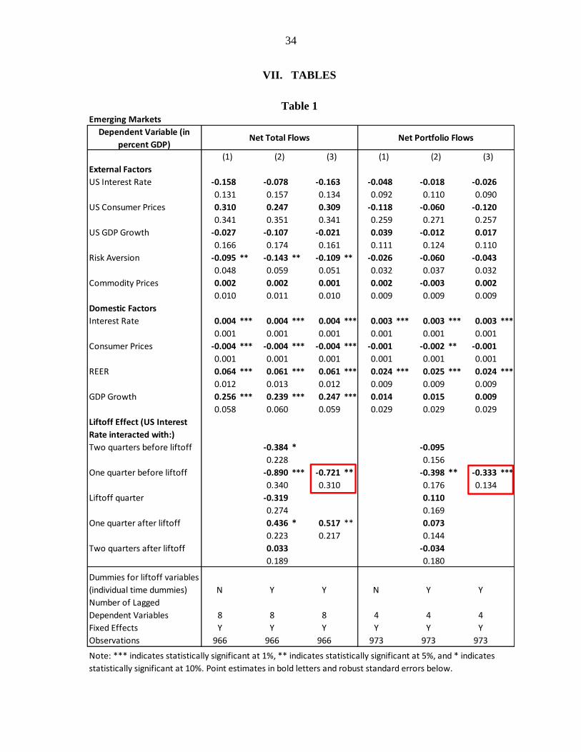
Using the empirical strategy discussed in the previous sub-section, table 1 reports the

first set of results for EM. The first three columns report the results for the three steps using

net total flows, as a share of GDP, as the dependent variable, while the last three columns

report the results using net portfolio flows, as a share of GDP, as the dependent variable. The

independent variables are grouped in three categories: the external factors (representing the

push factors), the domestic factors (representing the pull factors), and the liftoff variables

(the dummy variables interacted with the U.S. interest rate).

The first column for both total and portfolio flows shows that risk aversion and

domestic factors are significant determinants of capital flows. However, when the sample

excluding extreme data points is used, policy rates and inflation are not significant for total

flows and inflation and growth are no longer significant for portfolio flows. Similarly, in the

second and third column, some of the coefficients of the variables without liftoff effect (that

is, variables not interacted with the dummy variables) can be sensitive to extreme data points.

However, the coefficients of the interactive terms, representing the liftoff effects, are similar

in all the versions including/excluding extreme data points. Since the focus of the paper is on

the liftoff effect and the coefficients of the liftoff effect are similar in all the robustness

checks, this does not affect the main findings of the paper.

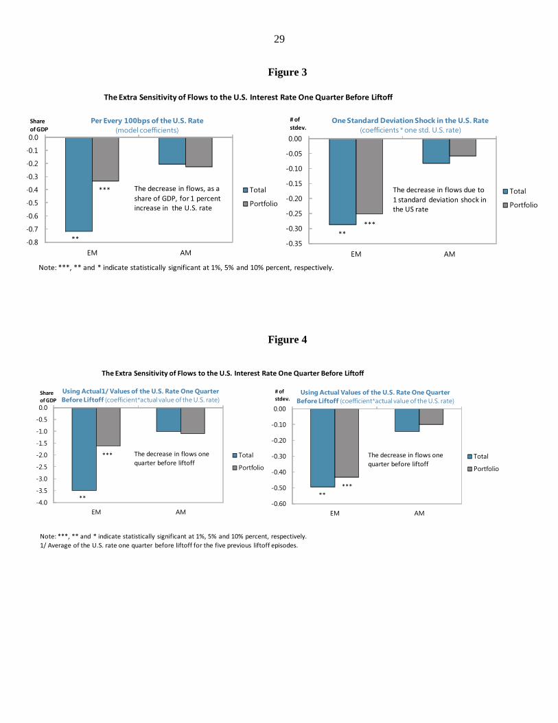
Turning to the focus of the paper, the results of the second and third column, using

both total and portfolio flows, clearly show that there is a significant liftoff effect of the U.S.

interest rate one quarter before liftoff – the variable capturing the interaction between the

dummy variable representing one quarter before liftoff and the U.S. interest rate is significant

in both cases. For every 100bps of the U.S. interest rate, there is 0.72 and 0.33 percent of

GDP of net total and net portfolio outflow, respectively, one quarter prior to the liftoff.

12

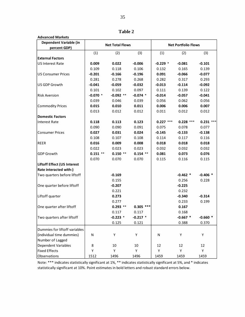
This liftoff effect of the U.S. rate seems to be absent for AM, as shown in table 2

where the same exercise is performed using AM instead of EM, and the next sub-section

shows that the magnitude is also less than EM (figures 3 and 4). There could be few possible

reasons for the diverging results between EM and AM. First, this could be due to the varying

reaction of capital flows during risk sell-off episodes. EM typically experience capital

outflows during risk sell-off; while AM, especially safe heavens, tend to receive capital

inflow. Second, AM tend to borrow in domestic currency while most EM borrow in US

dollars, making them more vulnerable to increases in the U.S. rate.

The results are, broadly speaking, robust to alternative specifications discussed in the

previous sub-section. In particular, the liftoff effect on EM portfolio flows is robust to all the

specifications listed, and in most cases, the coefficients are larger. Hence, the reported results

can be regarded as conservative estimates. However, the results on EM total flows in some

cases do not hold strongly.

Using Model Results to Get a Sense of Magnitude

The reported coefficients give a sense of the extra marginal impact of the U.S. rate on

capital flows during liftoff episodes – this is termed as the liftoff effect in the paper. To get a

sense of what could potentially be the extra total impact of a particular variable due to the

liftoff, the model results are used to perform two exercises. First, the coefficients are used to

compute the extra impact assuming a scenario with one standard deviation shock in the U.S.

rate. This is essentially the model coefficients multiplied by one standard deviation of the

U.S. rate. In other words, all else equal, what would be the extra impact on capital flows

during liftoff episodes (compared to normal times) due to one standard deviation shock in the

U.S. rate? Second, the coefficients are multiplied by the average values of the U.S. rate in the

past five episodes to get a sense of the model prediction of the extra total impact on capital

flows due to the liftoff. Again, this would answer the question that, all else equal, what was

the extra impact during liftoff episodes due to the level of the U.S. rate? It must be cautioned

that these exercises can give only an approximate idea of magnitude; hence, the numbers

should not be over-interpreted. The purpose is to get a sense of magnitude due to the liftoff

effect by performing two exercises that, put together, can give the reader an approximate

sense of the ranges of the possible impact on capital flows due to the liftoff.

13

The computations from the first exercise show that one standard deviation shock in

the U.S. interest rate would decrease the flows by 2.0 and 0.9 percent of GDP for total and

portfolio flows, respectively. When expressed in number of standard deviations of the

respective data, these numbers translate to equal magnitude, around 0.3 standard deviations

(figure 3). Using the average of the U.S. rate for every quarter before liftoff in the sample,

the results imply that, the previous liftoffs resulted in net outflow of 3.5 and 1.6 percent of

GDP for total and portfolio flows, respectively (figure 4). In standard deviation terms, these

numbers amount to 0.5 and 0.4. For total flows, there seems to be payback one quarter post

liftoff, though the magnitude is less than the loss before liftoff (table 1).

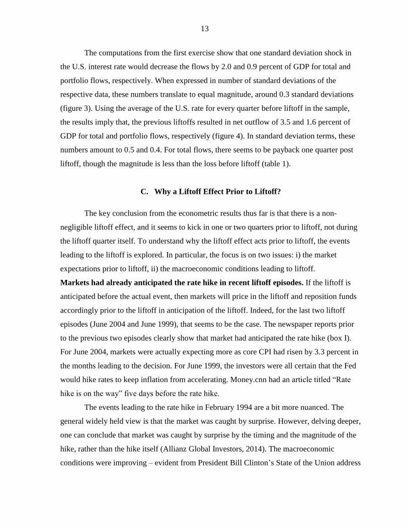
C. Why a Liftoff Effect Prior to Liftoff?

The key conclusion from the econometric results thus far is that there is a non-

negligible liftoff effect, and it seems to kick in one or two quarters prior to liftoff, not during

the liftoff quarter itself. To understand why the liftoff effect acts prior to liftoff, the events

leading to the liftoff is explored. In particular, the focus is on two issues: i) the market

expectations prior to liftoff, ii) the macroeconomic conditions leading to liftoff.

Markets had already anticipated the rate hike in recent liftoff episodes. If the liftoff is

anticipated before the actual event, then markets will price in the liftoff and reposition funds

accordingly prior to the liftoff in anticipation of the liftoff. Indeed, for the last two liftoff

episodes (June 2004 and June 1999), that seems to be the case. The newspaper reports prior

to the previous two episodes clearly show that market had anticipated the rate hike (box I).

For June 2004, markets were actually expecting more as core CPI had risen by 3.3 percent in

the months leading to the decision. For June 1999, the investors were all certain that the Fed

would hike rates to keep inflation from accelerating. Money.cnn had an article titled “Rate

hike is on the way” five days before the rate hike.

The events leading to the rate hike in February 1994 are a bit more nuanced. The

general widely held view is that the market was caught by surprise. However, delving deeper,

one can conclude that market was caught by surprise by the timing and the magnitude of the

hike, rather than the hike itself (Allianz Global Investors, 2014). The macroeconomic

conditions were improving – evident from President Bill Clinton’s State of the Union address

14

in January 1994 – and the then Fed Chairman Greenspan was hinting at potential rate hikes

for some time.

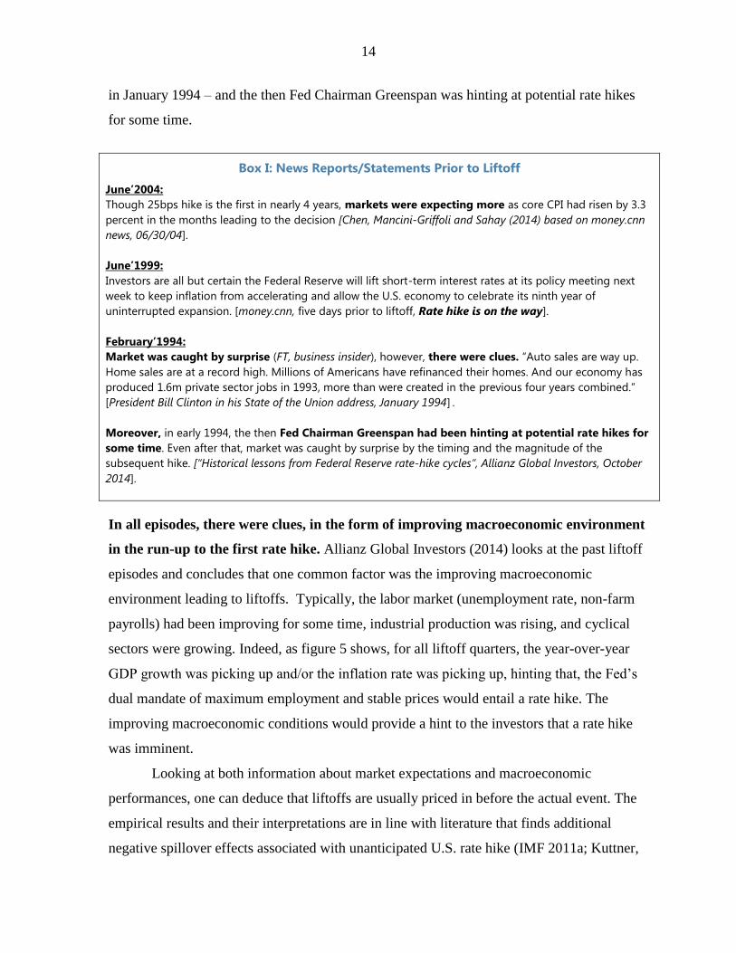
Box I: News Reports/Statements Prior to Liftoff

June’2004:

Though 25bps hike is the first in nearly 4 years, markets were expecting more as core CPI had risen by 3.3

percent in the months leading to the decision [Chen, Mancini-Griffoli and Sahay (2014) based on money.cnn

news, 06/30/04].

June’1999:

Investors are all but certain the Federal Reserve will lift short-term interest rates at its policy meeting next

week to keep inflation from accelerating and allow the U.S. economy to celebrate its ninth year of

uninterrupted expansion. [money.cnn, five days prior to liftoff, Rate hike is on the way].

February’1994:

Market was caught by surprise (FT, business insider), however, there were clues. “Auto sales are way up.

Home sales are at a record high. Millions of Americans have refinanced their homes. And our economy has

produced 1.6m private sector jobs in 1993, more than were created in the previous four years combined.”

[President Bill Clinton in his State of the Union address, January 1994] .

Moreover, in early 1994, the then Fed Chairman Greenspan had been hinting at potential rate hikes for

some time. Even after that, market was caught by surprise by the timing and the magnitude of the

subsequent hike. [“Historical lessons from Federal Reserve rate-hike cycles”, Allianz Global Investors, October

2014].

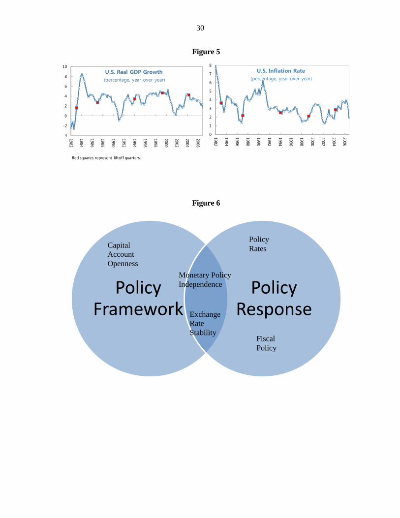
In all episodes, there were clues, in the form of improving macroeconomic environment

in the run-up to the first rate hike. Allianz Global Investors (2014) looks at the past liftoff

episodes and concludes that one common factor was the improving macroeconomic

environment leading to liftoffs. Typically, the labor market (unemployment rate, non-farm

payrolls) had been improving for some time, industrial production was rising, and cyclical

sectors were growing. Indeed, as figure 5 shows, for all liftoff quarters, the year-over-year

GDP growth was picking up and/or the inflation rate was picking up, hinting that, the Fed’s

dual mandate of maximum employment and stable prices would entail a rate hike. The

improving macroeconomic conditions would provide a hint to the investors that a rate hike

was imminent.

Looking at both information about market expectations and macroeconomic

performances, one can deduce that liftoffs are usually priced in before the actual event. The

empirical results and their interpretations are in line with literature that finds additional

negative spillover effects associated with unanticipated U.S. rate hike (IMF 2011a; Kuttner,

15

2001). Since the rate hike is usually priced in by the quarter of the liftoff, the liftoff effect of

the liftoff quarter is insignificant. However, as investors start to digest incoming data

showing improved macroeconomic conditions, they start building expectations and re-

positioning funds away from emerging markets – hence, the liftoff effect occurs before the

actual event.

III. THE LIFTOFF EFFECT OF DOMESTIC POLICIES

The previous section showed that the liftoff is usually accompanied by net capital

outflows as the sensitivity of flows to the U.S. rate increases in the quarter before liftoff. Can

domestic policies mitigate the negative effect of the Fed liftoff? This section aims to answer

that. Conceptually, a useful way of looking into policies would be to divide them into policy

responses and policy framework, with the understanding that there is room for overlap

between the two (figure 6). The policy response in a particular country would be a function

of the underlying policy framework. This sections looks at five areas domestic poly

responses/framework. First, the description of the policies are given, followed by the

empirical strategy used to include them in the regression specification. Finally, the results are

reported, followed by a discussion on the relative magnitude of the liftoff effects owing to the

U.S. rate hike and the policy responses/framework.

A. The Policies

To understand the role of domestic policies in mitigating the negative liftoff effect

emanating from the U.S. interest rate hike, the following five policies are looked at:

Domestic Policy Rates – In the face of the U.S. rate hike, can increasing domestic policy

rates retain capital flows by maintaining the interest rate differentials? The same policy rate

as the one in the generic model is used to understand this question. To capture the extra

liftoff effect pertaining to domestic policy rates, the interactive term with the liftoff dummies

are used.

16

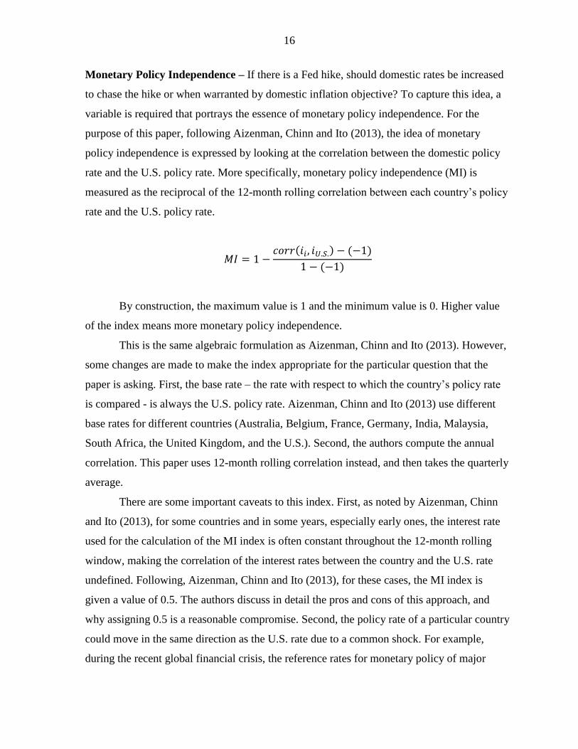
Monetary Policy Independence – If there is a Fed hike, should domestic rates be increased

to chase the hike or when warranted by domestic inflation objective? To capture this idea, a

variable is required that portrays the essence of monetary policy independence. For the

purpose of this paper, following Aizenman, Chinn and Ito (2013), the idea of monetary

policy independence is expressed by looking at the correlation between the domestic policy

rate and the U.S. policy rate. More specifically, monetary policy independence (MI) is

measured as the reciprocal of the 12-month rolling correlation between each country’s policy

rate and the U.S. policy rate.

By construction, the maximum value is 1 and the minimum value is 0. Higher value

of the index means more monetary policy independence.

This is the same algebraic formulation as Aizenman, Chinn and Ito (2013). However,

some changes are made to make the index appropriate for the particular question that the

paper is asking. First, the base rate – the rate with respect to which the country’s policy rate

is compared - is always the U.S. policy rate. Aizenman, Chinn and Ito (2013) use different

base rates for different countries (Australia, Belgium, France, Germany, India, Malaysia,

South Africa, the United Kingdom, and the U.S.). Second, the authors compute the annual

correlation. This paper uses 12-month rolling correlation instead, and then takes the quarterly

average.

There are some important caveats to this index. First, as noted by Aizenman, Chinn

and Ito (2013), for some countries and in some years, especially early ones, the interest rate

used for the calculation of the MI index is often constant throughout the 12-month rolling

window, making the correlation of the interest rates between the country and the U.S. rate

undefined. Following, Aizenman, Chinn and Ito (2013), for these cases, the MI index is

given a value of 0.5. The authors discuss in detail the pros and cons of this approach, and

why assigning 0.5 is a reasonable compromise. Second, the policy rate of a particular country

could move in the same direction as the U.S. rate due to a common shock. For example,

during the recent global financial crisis, the reference rates for monetary policy of major

17

central banks comoved quite strongly, not because they were following the Fed, but because

they were hit by a common shock. However, this might be less of an issue for this paper

since the period of analysis is until 2006, and hence does not include the global financial

crisis.

Exchange Rate Stability – Again, following Aizenman, Chinn and Ito (2013), a very simple

expression is used to capture the exchange rate stability of a particular country. The volatility

of the month-over-month exchange rate movements are used to understand the exchange rate

stability, with the idea that a more fixed exchange rate regime would have less volatility, and

vice versa. More specifically, the exchange rate stability index (ERS) is defined as the 12-

month rolling standard deviation of the monthly exchange rate change, and included in the

formula below to normalize the index between 0 and 1.

A higher value of the index indicates more stable movement of the exchange rate. Again,

Aizenman, Chinn and Ito (2013) use the exchange rate movement vis-à-vis a base country

which is not necessarily always the U.S. However, this paper uses the bilateral exchange rate

of the recipient country vis-à-vis the U.S dollar. The paper uses the 12-month rolling

standard deviation of currency movements whereas Aizenman, Chinn and Ito (2013) use

annual standard deviations of the monthly exchange rate changes.

Capital Account Openness – Are countries with more open capital account more prone to

liftoff effects? To answer this question, the widely used Chinn-Ito Index for capital account

openness is used. This index is based on information regarding restrictions in the IMF’s

Annual Report on Exchange Arrangements and Exchange Restrictions (AREAER). Chinn

and Ito (2006) provide a detailed description of the index. This index is normalized between

0 and 1, with higher value indicating that a country is open to cross-border capital

transactions.

18

Budget Surplus (Deficit) – Fiscal policy is one of the key policy tools available to the

government. In the face of a U.S. liftoff, one near-term policy response could be to improve

budget deficit to provide a positive signal to the market, particularly if a country’s fiscal

sustainability is an issue. In order to understand if fiscal policy can play any role in

mitigating the negative liftoff effect owing to the U.S. rate hike, the quarter over quarter

budget surplus, expressed as a share of GDP, is used. An increase in the variable means more

budget surplus, suggesting, all else equal, more fiscal discipline.

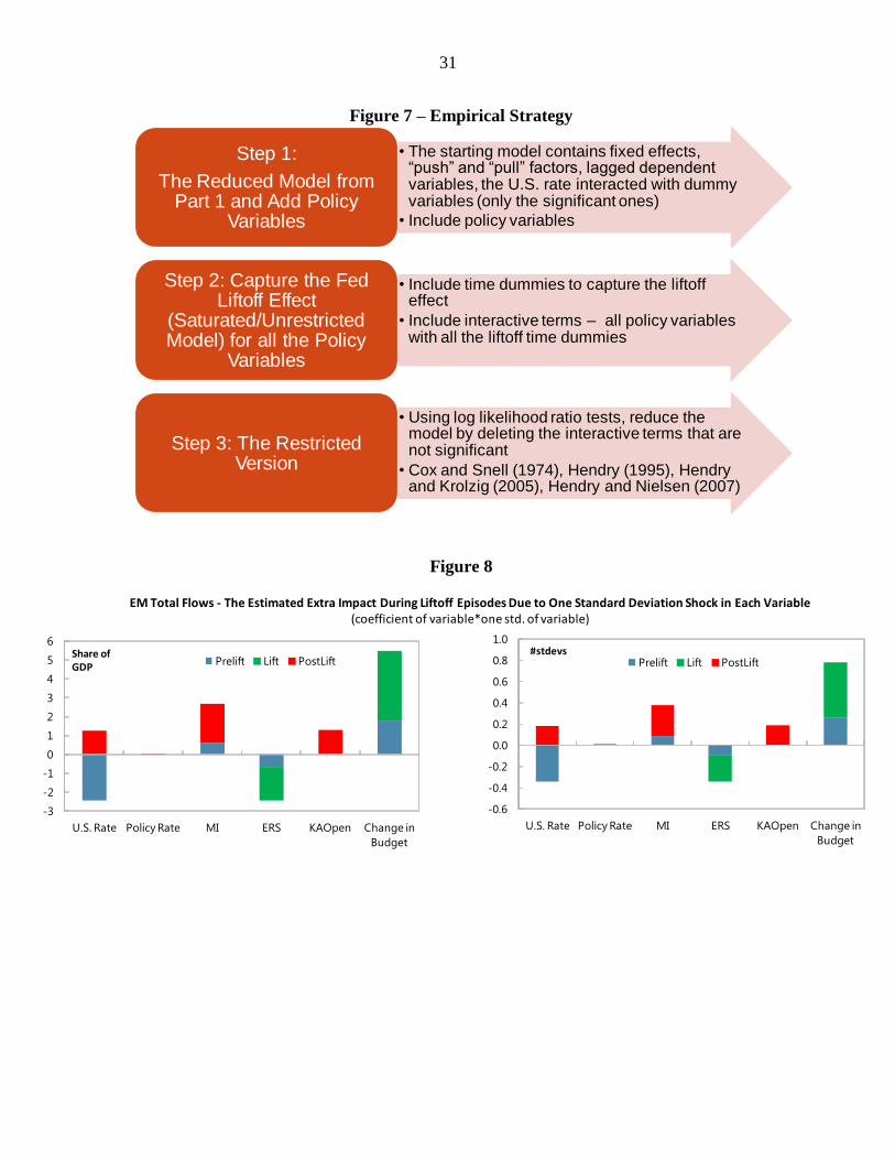
B. Empirical Strategy

Similar to the empirical strategy employed when measuring the liftoff effect of the

U.S. rate, a 3-step approach is used (figure 7).

The first step starts with the reduced model from the previous section containing

country specific fixed effects, “push” and “pull” factors, lagged dependent variables, the U.S.

rate interacted with dummy variables (only the significant ones), and the corresponding time

dummy variables. All the variables representing policy responses/framework, except budget

surplus, are included in this model.

In the second step, all the possible liftoff effects of all the policy variables are

included to obtain the saturated model. For each policy variable, the interactive term between

the policy variable and each time dummy is included. In other words, there are five

interactive terms for each policy variable showing the interaction with two quarters before

liftoff, one quarter before liftoff, liftoff quarter, one quarter after liftoff, and two quarters

after liftoff. In addition, all the time dummy variables are included. Like the previous section,

the liftoff effect of a particular variable is thus the coefficient of the interactive term

comprising the time dummy and the variable. The dummy variable in the interactive term

helps to identify if the liftoff effect occurs before, during and/or after liftoff.

For the third and the final step, the restricted version is obtained from the saturated

model by deleting the interactive terms that are not significant. Log-likelihood ratio tests are

also performed to make sure that the reduced version is preferred to the saturated model.

Since the data set for budget surplus is considerably shorter than the other policy

variables, the regressions for budget surplus are run separately, using the same 3-step

approach. The starting model contains the country specific fixed effects, “push” and “pull”

19

factors, lagged dependent variables, the U.S. rate interacted with dummy variables (only the

significant ones), the corresponding time dummy variables, and budget surplus. This model

is extended to include all the interactive terms between the budget surplus and the time

dummies. The final restricted version includes only the interactive terms that are statistically

significant. Log-likelihood ratio tests are performed to make sure the restricted version is

accepted against the saturated model.

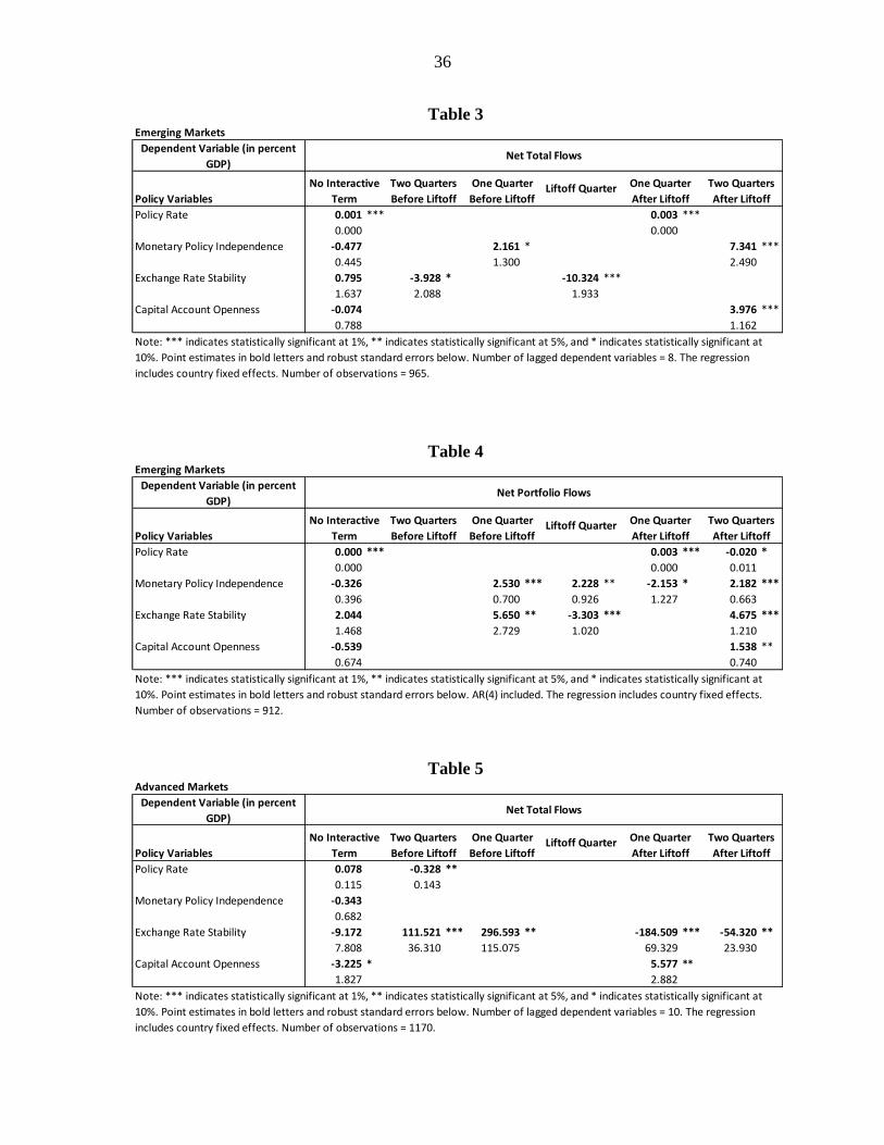
C. Results

This sub-section discusses the significance of the results. The magnitude is discussed

in the next sub-section. The coefficients of the policy variables and their interactive terms

with the dummy variables are reported in tables 3, 4, 5, and 6 for EM total flows, EM

portfolio flows, AM total flows, and AM portfolio flows, respectively. The results for fiscal

policies are reported separately in table 7.

Some overall observations strike out. First, the liftoff effects of policies are

substantially higher for EM than AM. Second, whereas the liftoff effect of the U.S. rate kicks

in before liftoff, that of the variables representing policy responses/framework usually act

during or after liftoff. Third, though the policy variables (with the exception of policy rates)

are not significant on their own, indicating they are not significant during normal times, they

are significant when interacted with liftoff dummies. This shows that, some of the policy

responses/framework, though not the usual determinant of capital flows, can be significant

during liftoff episodes. Looking at specific policy framework/response:

Monetary policy independence: The results indicate that keeping monetary policy

independence can help to increase net capital flows during liftoff episodes. Aizenman, Chinn

and Ito (2013) find that greater monetary policy independence can dampen output volatility.

The statistical significance of monetary policy independence could thus also reflect the

indirect impact of less output volatility on capital flows. The policy implication would be to

adjust monetary policy according to domestic inflation objectives. This finding is in line with

recent literature. IMF (2014) shows that monetary policy was one of the most used tools

during the taper tantrum episode. However, the report underscores that most countries raised

rates to fight against inflation, not just capital outflows and depreciating currencies. If rates

20

are increased for the latter purposes, the study cautions that they risk the opposite effects of

slowing down the economy, thereby undermining investor confidence, and in turn driving

further capital outflows and currency depreciation. In the same vein, a recent study (Goldman

Sachs, 2015) shows that the Asian Central Banks followed fundamentals, not the Fed, when

tightening in the mid-2000s.

Domestic policy rates: Though the reported results show that some interactive terms between

domestic policy rates and dummy variables are significant, they do not survive the robustness

tests. In particular, policy rates do not come out significant when extreme data points

(independent variables) are removed from the sample. Hence, one can conclude that there is

very weak or no evidence that raising policy rates helps during liftoff episodes.

Budget surplus: Interestingly, near term budget improvement – expressed in the regression as

quarter-over-quarter change in budget surplus (as a share of GDP) – comes out significant

even though near term budget surplus is not significant without the interactive term. Even

though fiscal policy is not a usual determinant of capital flows, the results suggest that it

could be an important tool during liftoff episodes. This result is very robust to all the

robustness checks mentioned previously. However, the results do not hold when budget

surplus, as a share of GDP, is expressed as year-over-year change. One possible explanation,

for the strong robust significance of the quarter-over-quarter budget surplus (but not year-

over-year budget surplus change) could come from the lessons during taper tantrum. IMF

(2014) finds that emerging markets that acted early and decisively have tended to fare better.

Improvement in the budget surplus could be an early signal to the market that policies are

committed towards improving fundamentals.

Capital account openness: One of the most interesting results of the paper is the lack of

statistical significance of capital account openness prior or during liftoff. The results show no

evidence that countries with more open capital accounts are hit more. This finding is in

accord with some recent literature that shows that domestic policies cannot do much to

attenuate spillovers during U.S. monetary policy shocks. Fratzscher, LoDuca and Straub

(2012) find no evidence that foreign exchange or capital account policies help contain

21

spillovers. However, the reported results in this paper show that countries with more open

capital accounts recover quicker: there is a statistically significant positive liftoff effect one

or two quarter after liftoff.

Exchange rate stability: Exchange rate stability is the only variable that shows significant

liftoff effect for AM5. The results for AM indicate that countries with more flexible exchange

rate regimes fare better in attracting capital flows post liftoff. The results for EM are more

mixed and not necessarily significant in terms of magnitude (see next sub-section). Countries

with more stable exchange rate seem to have more net total outflows two quarters before

liftoff and during the liftoff quarter. Countries with more stable exchange rate also have more

portfolio outflows during the liftoff quarter. However, more stable currency also attracts

more portfolio inflows one quarter prior to liftoff and two quarter post liftoff.

D. Can Policies Mitigate the Negative Liftoff Effect of the U.S. Rate?

This section discusses the potential magnitude of the results. The aim is to get an idea

if the policy framework/responses can make a meaningful difference. In particular, can they

mitigate the negative liftoff effect of the U.S. rate?6 The same two exercises, as in the

previous section, are performed, and the caveats already mentioned in that section also hold

here. The first looks at the extra impact on capital flows during liftoff episodes from one

standard deviation shock of each variable. The second exercise computes the extra impact by

taking average of the model predictions in the past five liftoff episodes (model coefficient

multiplied by the average values of the variables in the past episodes).

5 The only exception is the interactive term of the domestic policy rate that comes out significant two quarters

post liftoff for AM portfolio flows.

6 Since the spillover effects of the U.S. rate on AM is very limited and the policy response/framework seem not

to make any difference, evident from the lack of significant results in tables 5 and 6, this sections focuses on

EM only.

22

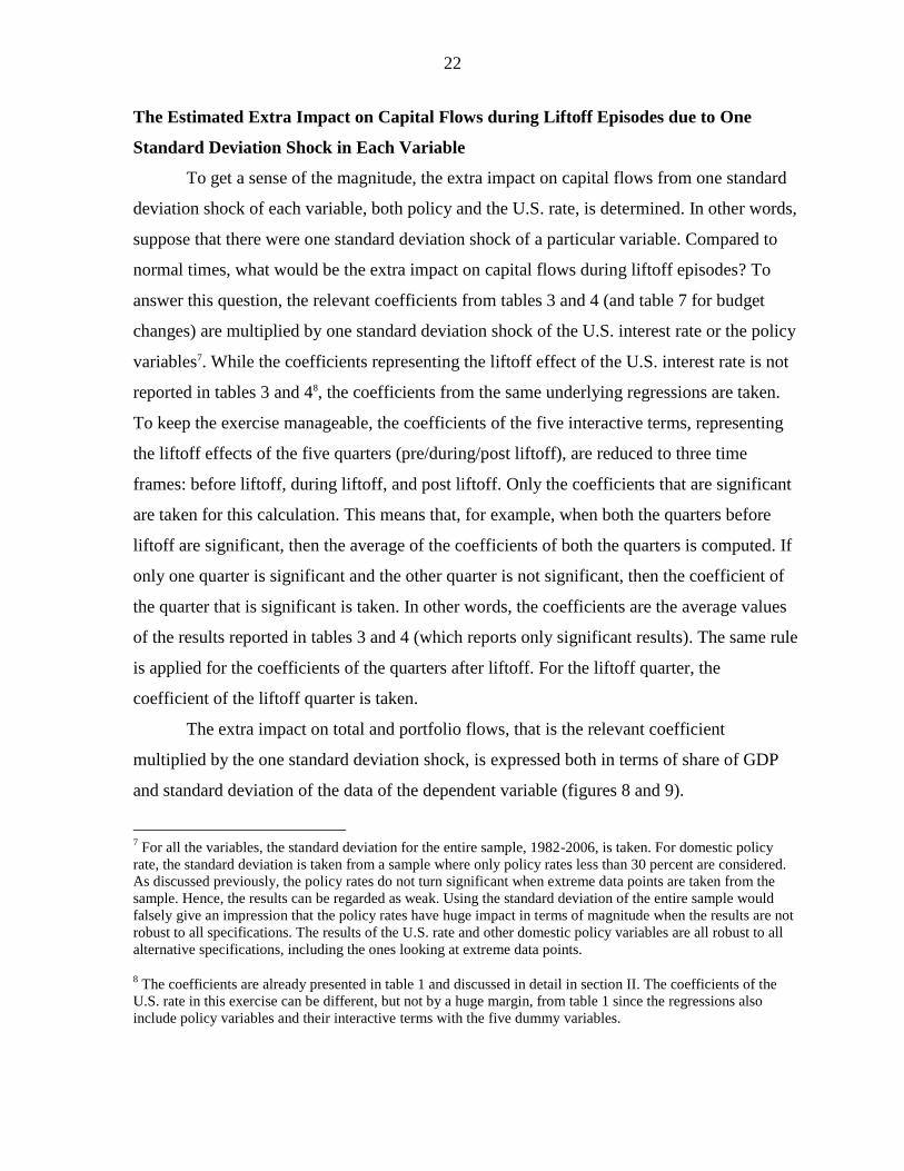
The Estimated Extra Impact on Capital Flows during Liftoff Episodes due to One

Standard Deviation Shock in Each Variable

To get a sense of the magnitude, the extra impact on capital flows from one standard

deviation shock of each variable, both policy and the U.S. rate, is determined. In other words,

suppose that there were one standard deviation shock of a particular variable. Compared to

normal times, what would be the extra impact on capital flows during liftoff episodes? To

answer this question, the relevant coefficients from tables 3 and 4 (and table 7 for budget

changes) are multiplied by one standard deviation shock of the U.S. interest rate or the policy

variables7. While the coefficients representing the liftoff effect of the U.S. interest rate is not

reported in tables 3 and 48, the coefficients from the same underlying regressions are taken.

To keep the exercise manageable, the coefficients of the five interactive terms, representing

the liftoff effects of the five quarters (pre/during/post liftoff), are reduced to three time

frames: before liftoff, during liftoff, and post liftoff. Only the coefficients that are significant

are taken for this calculation. This means that, for example, when both the quarters before

liftoff are significant, then the average of the coefficients of both the quarters is computed. If

only one quarter is significant and the other quarter is not significant, then the coefficient of

the quarter that is significant is taken. In other words, the coefficients are the average values

of the results reported in tables 3 and 4 (which reports only significant results). The same rule

is applied for the coefficients of the quarters after liftoff. For the liftoff quarter, the

coefficient of the liftoff quarter is taken.

The extra impact on total and portfolio flows, that is the relevant coefficient

multiplied by the one standard deviation shock, is expressed both in terms of share of GDP

and standard deviation of the data of the dependent variable (figures 8 and 9).

7 For all the variables, the standard deviation for the entire sample, 1982-2006, is taken. For domestic policy

rate, the standard deviation is taken from a sample where only policy rates less than 30 percent are considered.

As discussed previously, the policy rates do not turn significant when extreme data points are taken from the

sample. Hence, the results can be regarded as weak. Using the standard deviation of the entire sample would

falsely give an impression that the policy rates have huge impact in terms of magnitude when the results are not

robust to all specifications. The results of the U.S. rate and other domestic policy variables are all robust to all

alternative specifications, including the ones looking at extreme data points.

8 The coefficients are already presented in table 1 and discussed in detail in section II. The coefficients of the

U.S. rate in this exercise can be different, but not by a huge margin, from table 1 since the regressions also

include policy variables and their interactive terms with the five dummy variables.

23

For total flows, the results indicate that before liftoff, the net outflow due to one

standard deviation shock in the U.S. rate could be substantial, around 2.4 percent of GDP

(0.3 standard deviation of the data). This effect cannot be completely mitigated by policy

variables before liftoff. Only one standard deviation shock of the quarterly improvement in

budget could help by attracting net inflow of 1.8 percent of GDP. During the liftoff quarter,

improvement in quarterly budget surplus can give substantial boost, attracting around net

inflows of 3.7 percent of GDP. After liftoff, monetary policy independence and open capital

accounts can help, attracting net inflows of 2.1 and 1.3 percent of GDP, respectively.

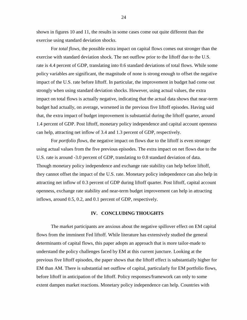
For portfolio flows, the results indicate that before liftoff, the net outflow due to one

standard deviation shock in the U.S. rate could be substantial, around 1.7 percent of GDP.

This translates into 0.5 standard deviation of the data, higher than the standard deviation

reported for total flows. Unlike total flows, a positive shock in near-term budget does not

have an impact before liftoff. However, monetary policy independence and exchange rate

stability shocks can help to some extent. During liftoff quarter, maintaining monetary policy

independence can help by attracting net inflow of 0.6 percent of GDP. However, countries

with more fixed exchange rate seem to be hit more, with a net outflow of 0.6 percent of GDP.

After liftoff, near-term budget improvement, exchange rate stability, and capital account

openness shocks can increase net portfolio flows, by 1.3, 0.8 and 0.5 percent of GDP,

respectively.

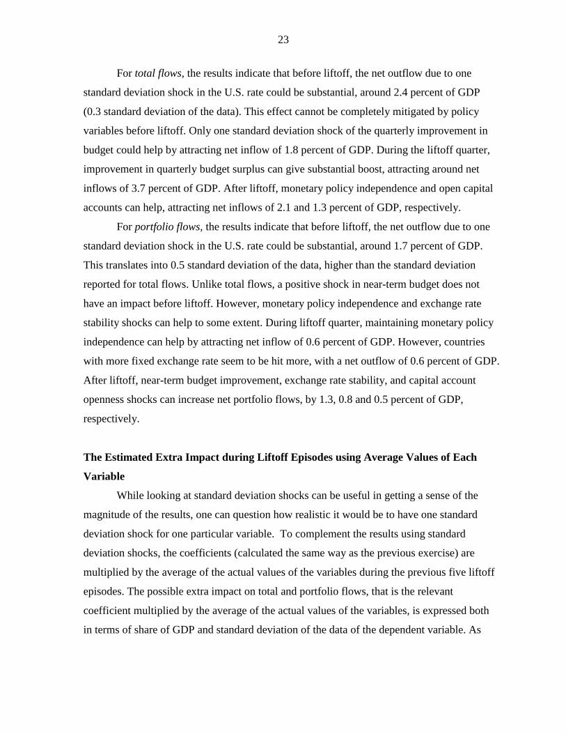
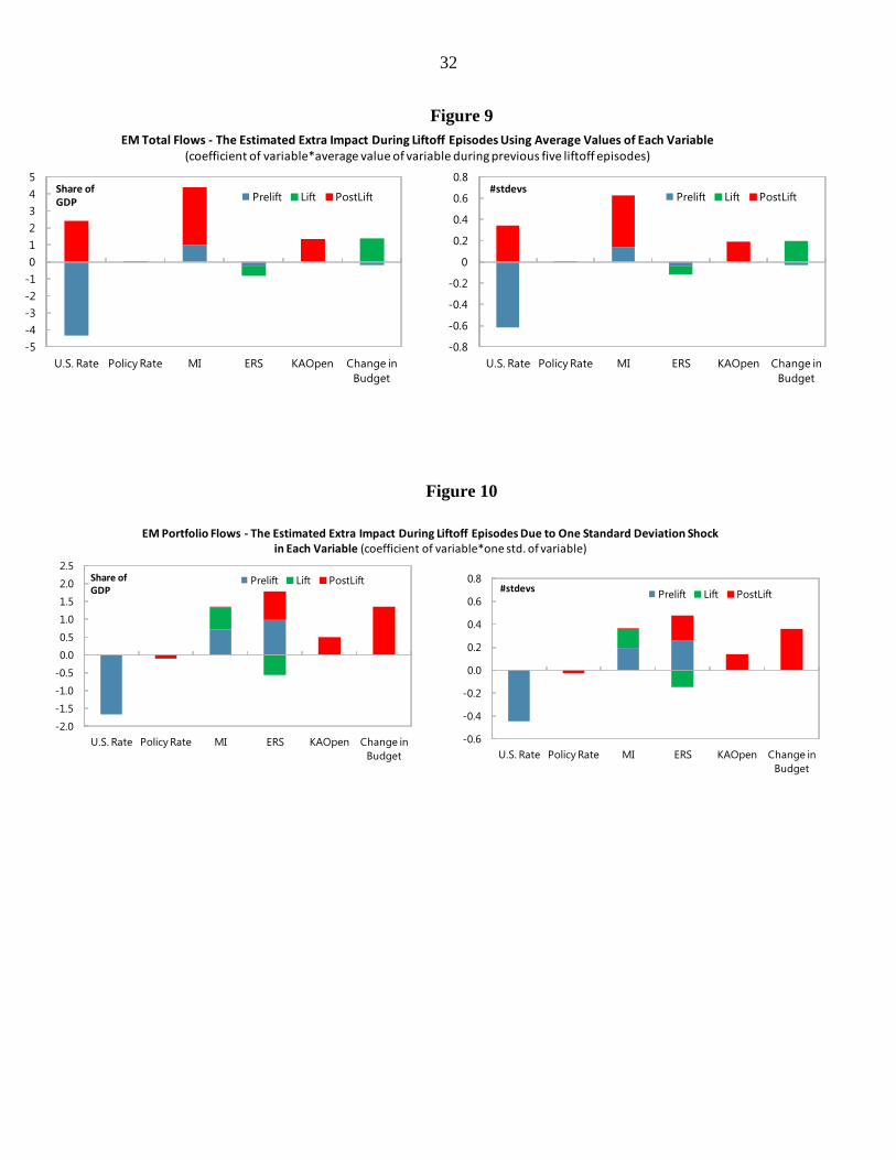
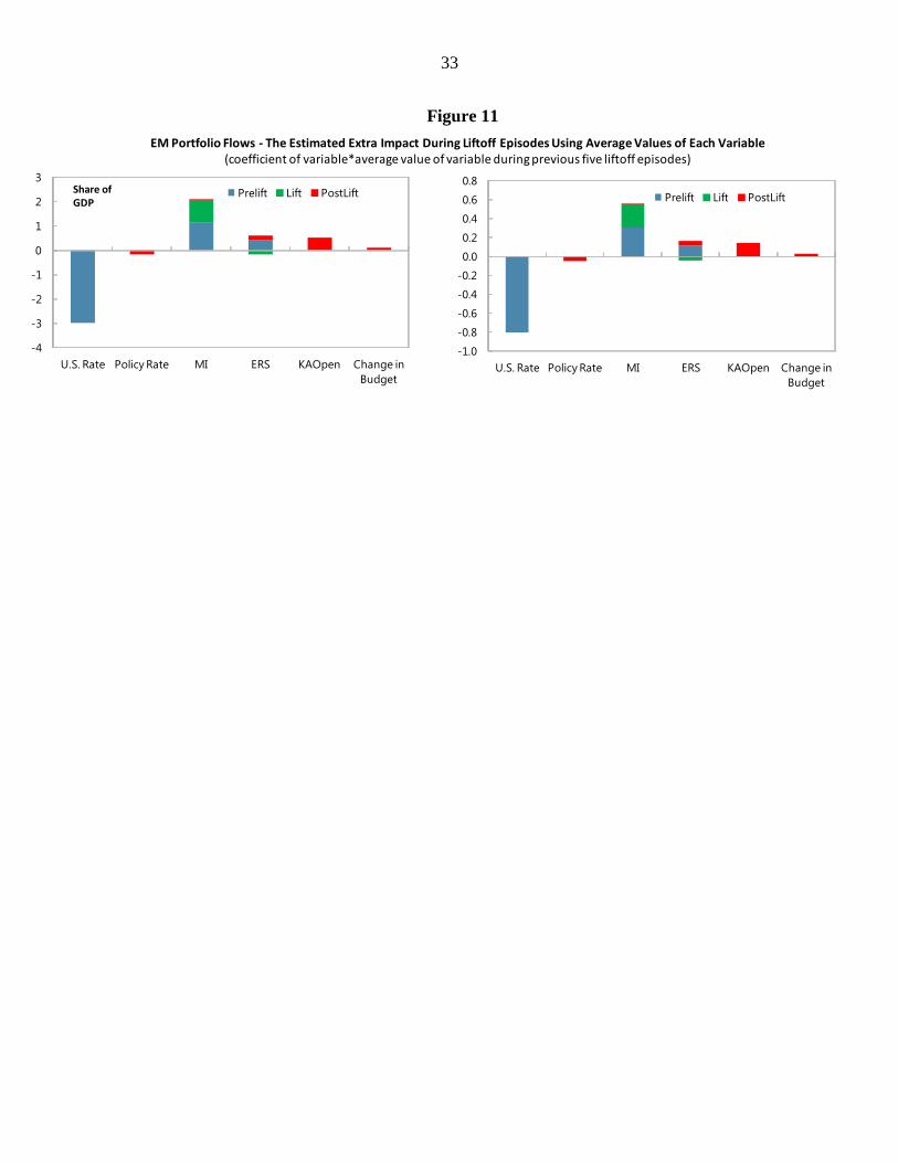
The Estimated Extra Impact during Liftoff Episodes using Average Values of Each

Variable

While looking at standard deviation shocks can be useful in getting a sense of the

magnitude of the results, one can question how realistic it would be to have one standard

deviation shock for one particular variable. To complement the results using standard

deviation shocks, the coefficients (calculated the same way as the previous exercise) are

multiplied by the average of the actual values of the variables during the previous five liftoff

episodes. The possible extra impact on total and portfolio flows, that is the relevant

coefficient multiplied by the average of the actual values of the variables, is expressed both

in terms of share of GDP and standard deviation of the data of the dependent variable. As

24

shown in figures 10 and 11, the results in some cases come out quite different than the

exercise using standard deviation shocks.

For total flows, the possible extra impact on capital flows comes out stronger than the

exercise with standard deviation shock. The net outflow prior to the liftoff due to the U.S.

rate is 4.4 percent of GDP, translating into 0.6 standard deviations of total flows. While some

policy variables are significant, the magnitude of none is strong enough to offset the negative

impact of the U.S. rate before liftoff. In particular, the improvement in budget had come out

strongly when using standard deviation shocks. However, using actual values, the extra

impact on total flows is actually negative, indicating that the actual data shows that near-term

budget had actually, on average, worsened in the previous five liftoff episodes. Having said

that, the extra impact of budget improvement is substantial during the liftoff quarter, around

1.4 percent of GDP. Post liftoff, monetary policy independence and capital account openness

can help, attracting net inflow of 3.4 and 1.3 percent of GDP, respectively.

For portfolio flows, the negative impact on flows due to the liftoff is even stronger

using actual values from the five previous episodes. The extra impact on net flows due to the

U.S. rate is around -3.0 percent of GDP, translating to 0.8 standard deviation of data.

Though monetary policy independence and exchange rate stability can help before liftoff,

they cannot offset the impact of the U.S. rate. Monetary policy independence can also help in

attracting net inflow of 0.3 percent of GDP during liftoff quarter. Post liftoff, capital account

openness, exchange rate stability and near-term budget improvement can help in attracting

inflows, around 0.5, 0.2, and 0.1 percent of GDP, respectively.

IV. CONCLUDING THOUGHTS

The market participants are anxious about the negative spillover effect on EM capital

flows from the imminent Fed liftoff. While literature has extensively studied the general

determinants of capital flows, this paper adopts an approach that is more tailor-made to

understand the policy challenges faced by EM at this current juncture. Looking at the

previous five liftoff episodes, the paper shows that the liftoff effect is substantially higher for

EM than AM. There is substantial net outflow of capital, particularly for EM portfolio flows,

before liftoff in anticipation of the liftoff. Policy responses/framework can only to some

extent dampen market reactions. Monetary policy independence can help. Countries with

25

higher monetary policy independence may have greater leeway at this current juncture. Since

monetary policy independence requires time, other countries could undertake reforms to

increase monetary policy independence in future. In terms of fiscal policy, reducing near-

term budget deficit can give a positive signal to the market and somewhat reduce capital

outflows for countries with credibility and fiscal sustainability issues. In terms of policy

framework, capital account openness does not lead to more outflows during or before liftoff.

However, capital account openness can help to attract capital flows after Fed liftoff.

While the paper looks at five areas of policy framework/response, this is not an

exhaustive list. Recent literature points to a host of factors that can help to reduce external

vulnerabilities. In particular, IMF (2014) shows that elevated current account deficits, high

inflation, weak growth prospects, and relatively low reserves exacerbated market reactions

during the taper tantrum episode. These factors can be addressed by policies that are not

necessarily included in this paper. Recent studies have also given a lot of focus on the impact

of macro prudential policies (Cerutti, Claessens and Laeven, 2015) – something not

addressed in this paper. For example, Dell’Ariccia et al. (2012) find that macroprudential

policies can reduce the incidence of general credit booms and decrease the probability that

booms end up badly. Zhang and Zoli (2014) and Bruno, Shim and Shin (2014) look at the

relationship between macroprudential policies and capital flow measures, and find that such

policies can slow inflows.

The general finding of this paper is that, before liftoff, EM capital flows are

indiscriminately hit across countries. Over time, there is more variation across countries as

individual policy responses/framework can to some extent dampen market reaction. This is

how things had unfolded during the taper tantrum episode (IMF, 2014) suggesting that

history can be a good guidance for the future liftoff. Some of the policies that can attract

capital flows (e.g. improving fiscal sustainability) can be pro-cyclical in the current juncture

where EM growth is slowing down considerably. Monetary policy independence is

associated with gaining credibility. This takes time and may not be done quickly in the

current environment. Also, monetary policy independence is easier said than done in the

current environment where EM currencies are under pressure. Hence, the findings of the

paper suggest that some EM face tough policy tradeoffs in the current situation. This is yet

another paper that suggests an important role for global institutions and cross-country

26

cooperation to deal with sharp volatility of capital flows (Forbes and Warnock, 2012) and

safeguard global financial stability (IMF, 2014).

V. REFERENCES

Ahmed, Shagil, and Andrei Zlate (2014). “Capital flows to emerging market economies: A brave new

world?”, Journal of International Money and Finance, 48: 221–248.

Aizenman, Joshua, Menzie D. Chinn, and Hiro Ito (2013). “The ‘Impossible Trinity’ Hypothesis in an

Era of Global Imbalances: Measurement and Testing”, Review of International Economics,

21(3), 447–458 (August 2013).

Allianz Global Investors (2014). “Historical lessons from Federal Reserve rate-hike cycles”,

http://www.allianzgi.com/en/Market-Insights/Pages/Historical-lessons-from-Federal-

Reserve-rate-hike-cycles.aspx.

Broner, Fernando, Tatiana Didier, Aitor Erce, and Sergio Schmukler (2013). “Gross capital flows:

Dynamics and crises”, Journal of Monetary Economics 60(1): 113–133.

Bruno, Valentina, Ilhyock Shim, and Hyun Song Shin (2014). “Comparative Assessment of

Macroprudential Policies”, Bank of International Settlements, October.

Calvo, Guillermo (1998). “Capital flows and capital-market crises: the simple economics of sudden

stops”, Journal of Applied Economics 1(1): 35–54.

Cerutti, Eugenio, Stijn Claessens, and Luc Laeven (2015). “The Use and Effectiveness of

Macroprudential Policies: New Evidence”, IMF Working Paper, WP/15/61.

Chen, Jiaqian, Tommaso Mancini-Griffoli and Ratna Sahay (2014). “Spillovers from United States

Monetary Policy on Emerging Markets: Different This Time?”, IMF Working Paper,

WP/14/240.

Chinn, Menzie D. and Hiro Ito (2006). “What Matters for Financial Development? Capital Controls,

Institutions, and Interactions”, Journal of Development Economics, 81(1), 163–192

(October).

Chuhan, Punam, Stijn Claessens, and Nlandu Mamingi (1993). “Equity and Bond Flows to Latin

America and Asia: The Role of Global and Cuntry Factors”, World Bank Policy Research,

Working Paper 1160.

Cox, David Roxbee and E. Joyce Snell (1974). "The choice of variables in observational studies",

Applied statistics, 23, 51–59.

27

Dell’Ariccia, Giovanni, Deniz Igan, Luc Laeven, and Hui Tong, with Bas Bakker and Jerome

Vandenbussche (2012). "Policies for MAcrofinancial Stability: How to Deal with Credit

Booms", IMF Staff Discussion Notes, 12/05.

Hendry, David F. and Bent Nielsen (2007). “Econometric Modeling: A Likelihood Approach”,

Princeton: Princeton University Press.

Hendry, David F. and Hans-Martin Krolzig (2005). "The properties of automatic Gets modelling",

Economic Journal, 115, C32–C61.

Hoover, Kevin D. and Stephen J. Perez (1999). "Data mining reconsidered: Encompassing and the

general-to-specific approach to specification search", Econometrics Journal, 2, 167–191.

Fernandez-Arias, Eduardo (1996). “The New Wave of Private Capital Inflows: Push or Pull?”,

Journal of Development Economics, 38(2), 389–418.

Fernandez-Arias, Eduardo, and Peter Montiel (1996). “The Surge in Capital Inflows to Developing

Countries: An Analytical Overview”, World Bank Economic Review, 10(1), 51–77.

Forbes, Kristin J., and Frank E. Warnock (2012). “Capital flow waves: surges, stops, flight, and

retrenchment”, Journal of International Economics, 88(2), 235–251.

Fratzscher, Marcel, Marco Lo Duca, and Roland Straub (2012). “A Global Monetary Tsunami?

On the Spillovers of U.S. Quantitative Easing”, CEPR Working Paper 9195.

Ghosh, Atish R., Mahvash S. Qureshi, Jun II Kim, and Juan Zalduendo (2014). “Surges”, Journal of

International Economics, 92(2), 266–285.

Goldman Sachs (2015). “Asian Central Banks followed fundamentals, not the Fed, when tightening in

the mid-2000s”, EM Macro Daily (July 20, 2015).

International Monetary Fund (2014). “Emerging Market Volatility: Lessons from the Taper

Tantrum”, Staff Discussion Note, SDN/14/09.

International Monetary Fund (2011a). “International Capital Flows: Reliable or Fickle?”, World

Economic Outlook, Chapter 4, April 2011.

International Monetary Fund (2011b). “Recent Experiences in Managing Capital Inflows – Cross-

Cutting Themes and Possible Policy Framework”, IMF Board Paper, February 14, 2011.

Kuttner, Kenneth N. (2001). “Monetary Policy Surprises and Interest Rates: Evidence from the Fed

Funds Futures Market”, Journal of Monetary Economics, 47(3), 523–44.

Zhang, Longmei and Edda Zoli (2014). “Leaning Against the Wind: Macroprudential Policy in Asia”,

IMF Working Paper 14/22.

28

VI. FIGURES

Figure 1 – Empirical Strategy

Figure 2

• External “push” factors and domestic “pull” factors

• Identify the variables using literature

• Lagged dependent variables, country fixed effects

Step 1:

Generic Model for Capital Flows

• Include time dummies to capture the liftoff effect

• Include interactive terms – U.S. rates with all the liftoff time dummies

Step 2: Capture the Fed Liftoff Effect

(Saturated/Unrestricted Model)

• Using log likelihood ratio tests, reduce the model by deleting the interactive terms that are not significant

• Cox and Snell (1974), Hendry (1995), Hendry and Krolzig (2005), Hendry and Nielsen (2007)

Step 3: The Restricted Version

0

4

8

12

16

1982

1983

1984

1985

1986

1987

1988

1989

1990

1991

1992

1993

1994

1995

1996

1997

1998

1999

2000

2001

2002

2003

2004

2005

2006

The Fed Liftoff Episodes

Federal Funds Effective Rate (%)

29

Figure 3

Figure 4

-0.8

-0.7

-0.6

-0.5

-0.4

-0.3

-0.2

-0.1

0.0

EM AM

Per Every 100bps of the U.S. Rate

(model coefficients)

Total

Portfolio

The decrease in flows, as a

share of GDP, for 1 percent increase in the U.S. rate

***

Share

of GDP

**

Note: ***, ** and * indicate statistically significant at 1%, 5% and 10% percent, respectively.

-0.35

-0.30

-0.25

-0.20

-0.15

-0.10

-0.05

0.00

EM AM

One Standard Deviation Shock in the U.S. Rate

(coefficients * one std. U.S. rate)

Total

Portfolio

The decrease in flows due to

1 standard deviation shock in the US rate

***

**

# of

stdev.

The Extra Sensitivity of Flows to the U.S. Interest Rate One Quarter Before Liftoff

-4.0

-3.5

-3.0

-2.5

-2.0

-1.5

-1.0

-0.5

0.0

EM AM

Using Actual1/ Values of the U.S. Rate One Quarter

Before Liftoff (coefficient*actual value of the U.S. rate)

Total

Portfolio

The decrease in flows one

quarter before liftoff***

Share

of GDP

**-0.60

-0.50

-0.40

-0.30

-0.20

-0.10

0.00

EM AM

Using Actual Values of the U.S. Rate One Quarter

Before Liftoff (coefficient*actual value of the U.S. rate)

Total

Portfolio

The decrease in flows one

quarter before liftoff

***

**

# of

stdev.

Note: ***, ** and * indicate statistically significant at 1%, 5% and 10% percent, respectively.

1/ Average of the U.S. rate one quarter before liftoff for the five previous liftoff episodes.

The Extra Sensitivity of Flows to the U.S. Interest Rate One Quarter Before Liftoff

30

Figure 5

Figure 6

-4

-2

0

2

4

6

8

10

1982

1984

1986

1988

1990

1992

1994

1996

1998

2000

2002

2004

2006

U.S. Real GDP Growth

(percentage, year-over-year)

0

1

2

3

4

5

6

7

8

1982

1984

1986

1988

1990

1992

1994

1996

1998

2000

2002

2004

2006

U.S. Inflation Rate

(percentage, year-over-year)

Red squares represent liftoff quarters.

Policy Framework

Policy Response

Capital

Account

Openness

Monetary Policy

Independence

Exchange

Rate

Stability

Policy

Rates

Fiscal

Policy

31

Figure 7 – Empirical Strategy

Figure 8

• The starting model contains fixed effects, “push” and “pull” factors, lagged dependent variables, the U.S. rate interacted with dummy variables (only the significant ones)

• Include policy variables

Step 1:

The Reduced Model from Part 1 and Add Policy

Variables

• Include time dummies to capture the liftoff effect

• Include interactive terms – all policy variables with all the liftoff time dummies

Step 2: Capture the Fed Liftoff Effect

(Saturated/Unrestricted Model) for all the Policy

Variables

• Using log likelihood ratio tests, reduce the model by deleting the interactive terms that are not significant

• Cox and Snell (1974), Hendry (1995), Hendry and Krolzig (2005), Hendry and Nielsen (2007)

Step 3: The Restricted Version

-3

-2

-1

0

1

2

3

4

5

6

U.S. Rate Policy Rate MI ERS KAOpen Change in

Budget

Prelift Lift PostLift

-0.6

-0.4

-0.2

0.0

0.2

0.4

0.6

0.8

1.0

U.S. Rate Policy Rate MI ERS KAOpen Change in

Budget

Prelift Lift PostLift

EM Total Flows - The Estimated Extra Impact During Liftoff Episodes Due to One Standard Deviation Shock in Each Variable (coefficient of variable*one std. of variable)

Share of GDP

#stdevs

32

Figure 9

Figure 10

-5

-4

-3

-2

-1

0

1

2

3

4

5

U.S. Rate Policy Rate MI ERS KAOpen Change in

Budget

Prelift Lift PostLiftShare of GDP

-0.8

-0.6

-0.4

-0.2

0

0.2

0.4

0.6

0.8

U.S. Rate Policy Rate MI ERS KAOpen Change in

Budget

Prelift Lift PostLift#stdevs

EM Total Flows - The Estimated Extra Impact During Liftoff Episodes Using Average Values of Each Variable (coefficient of variable*average value of variable during previous five liftoff episodes)

-2.0

-1.5

-1.0

-0.5

0.0

0.5

1.0

1.5

2.0

2.5

U.S. Rate Policy Rate MI ERS KAOpen Change in

Budget

Prelift Lift PostLift

-0.6

-0.4

-0.2

0.0

0.2

0.4

0.6

0.8

U.S. Rate Policy Rate MI ERS KAOpen Change in

Budget

Prelift Lift PostLift

Share of GDP #stdevs

EM Portfolio Flows - The Estimated Extra Impact During Liftoff Episodes Due to One Standard Deviation Shock in Each Variable (coefficient of variable*one std. of variable)

33

Figure 11

-4

-3

-2

-1

0

1

2

3

U.S. Rate Policy Rate MI ERS KAOpen Change in

Budget

Prelift Lift PostLiftShare of GDP

-1.0

-0.8

-0.6

-0.4

-0.2

0.0

0.2

0.4

0.6

0.8

U.S. Rate Policy Rate MI ERS KAOpen Change in

Budget

Prelift Lift PostLift

EM Portfolio Flows - The Estimated Extra Impact During Liftoff Episodes Using Average Values of Each Variable (coefficient of variable*average value of variable during previous five liftoff episodes)

34

VII. TABLES

Table 1

Emerging Markets

Dependent Variable (in

percent GDP)

External Factors

US Interest Rate -0.158 -0.078 -0.163 -0.048 -0.018 -0.026

0.131 0.157 0.134 0.092 0.110 0.090

US Consumer Prices 0.310 0.247 0.309 -0.118 -0.060 -0.120

0.341 0.351 0.341 0.259 0.271 0.257

US GDP Growth -0.027 -0.107 -0.021 0.039 -0.012 0.017

0.166 0.174 0.161 0.111 0.124 0.110

Risk Aversion -0.095 ** -0.143 ** -0.109 ** -0.026 -0.060 -0.043

0.048 0.059 0.051 0.032 0.037 0.032

Commodity Prices 0.002 0.002 0.001 0.002 -0.003 0.002

0.010 0.011 0.010 0.009 0.009 0.009

Domestic Factors

Interest Rate 0.004 *** 0.004 *** 0.004 *** 0.003 *** 0.003 *** 0.003 ***

0.001 0.001 0.001 0.001 0.001 0.001

Consumer Prices -0.004 *** -0.004 *** -0.004 *** -0.001 -0.002 ** -0.001

0.001 0.001 0.001 0.001 0.001 0.001

REER 0.064 *** 0.061 *** 0.061 *** 0.024 *** 0.025 *** 0.024 ***

0.012 0.013 0.012 0.009 0.009 0.009

GDP Growth 0.256 *** 0.239 *** 0.247 *** 0.014 0.015 0.009

0.058 0.060 0.059 0.029 0.029 0.029

Liftoff Effect (US Interest

Rate interacted with:)

Two quarters before liftoff -0.384 * -0.095

0.228 0.156

One quarter before liftoff -0.890 *** -0.721 ** -0.398 ** -0.333 ***

0.340 0.310 0.176 0.134

Liftoff quarter -0.319 0.110

0.274 0.169

One quarter after liftoff 0.436 * 0.517 ** 0.073

0.223 0.217 0.144

Two quarters after liftoff 0.033 -0.034

0.189 0.180

Dummies for liftoff variables

(individual time dummies) N Y Y N Y Y

Number of Lagged

Dependent Variables 8 8 8 4 4 4

Fixed Effects Y Y Y Y Y Y

Observations 966 966 966 973 973 973

Net Total Flows Net Portfolio Flows

Note: *** indicates statistically significant at 1%, ** indicates statistically significant at 5%, and * indicates

statistically significant at 10%. Point estimates in bold letters and robust standard errors below.

(1) (2) (3) (1) (2) (3)

35

Table 2

Advanced Markets

Dependent Variable (in

percent GDP)

External Factors

US Interest Rate 0.009 0.022 -0.006 -0.229 * -0.081 -0.101

0.109 0.118 0.106 0.132 0.165 0.139

US Consumer Prices -0.201 -0.166 -0.196 0.091 -0.066 -0.077

0.281 0.278 0.268 0.282 0.317 0.293

US GDP Growth -0.041 -0.059 -0.032 -0.013 -0.114 -0.092

0.101 0.102 0.097 0.111 0.139 0.122

Risk Aversion -0.070 * -0.092 ** -0.074 * -0.014 -0.057 -0.041

0.039 0.046 0.039 0.056 0.062 0.056

Commodity Prices 0.015 0.010 0.011 0.006 0.006 0.007

0.013 0.012 0.012 0.011 0.012 0.012

Domestic Factors

Interest Rate 0.118 0.113 0.123 0.227 *** 0.228 *** 0.231 ***

0.090 0.090 0.091 0.075 0.078 0.077

Consumer Prices 0.027 0.031 0.024 -0.145 -0.133 -0.138

0.108 0.107 0.108 0.114 0.117 0.116

REER 0.016 0.009 0.008 0.018 0.018 0.018

0.022 0.023 0.023 0.032 0.032 0.032

GDP Growth 0.151 ** 0.150 ** 0.154 ** 0.081 0.073 0.076

0.070 0.070 0.070 0.115 0.116 0.115

Liftoff Effect (US Interest

Rate interacted with:)

Two quarters before liftoff -0.169 -0.462 * -0.406 *

0.155 0.256 0.228

One quarter before liftoff -0.207 -0.225

0.221 0.232

Liftoff quarter 0.273 -0.340 -0.314

0.277 0.233 0.199

One quarter after liftoff 0.293 ** 0.305 *** 0.167

0.117 0.117 0.168

Two quarters after liftoff -0.223 * -0.217 * -0.667 * -0.660 *

0.125 0.121 0.388 0.370

Dummies for liftoff variables

(individual time dummies) N Y Y N Y Y

Number of Lagged

Dependent Variables 8 10 10 12 12 12

Fixed Effects Y Y Y Y Y Y

Observations 1512 1496 1496 1459 1459 1459

Note: *** indicates statistically significant at 1%, ** indicates statistically significant at 5%, and * indicates

statistically significant at 10%. Point estimates in bold letters and robust standard errors below.

Net Total Flows Net Portfolio Flows

(1) (2) (3) (1) (2) (3)

36

Table 3

Table 4

Table 5

Emerging Markets

Dependent Variable (in percent

GDP)

Policy Variables

Policy Rate 0.001 *** 0.003 ***

0.000 0.000

Monetary Policy Independence -0.477 2.161 * 7.341 ***

0.445 1.300 2.490

Exchange Rate Stability 0.795 -3.928 * -10.324 ***

1.637 2.088 1.933

Capital Account Openness -0.074 3.976 ***

0.788 1.162

One Quarter

After Liftoff

Two Quarters

After Liftoff

Net Total Flows

Note: *** indicates statistically significant at 1%, ** indicates statistically significant at 5%, and * indicates statistically significant at

10%. Point estimates in bold letters and robust standard errors below. Number of lagged dependent variables = 8. The regression

includes country fixed effects. Number of observations = 965.

No Interactive

Term

Two Quarters

Before Liftoff

One Quarter

Before LiftoffLiftoff Quarter

Emerging Markets

Dependent Variable (in percent

GDP)

Policy Variables

Policy Rate 0.000 *** 0.003 *** -0.020 *

0.000 0.000 0.011

Monetary Policy Independence -0.326 2.530 *** 2.228 ** -2.153 * 2.182 ***

0.396 0.700 0.926 1.227 0.663

Exchange Rate Stability 2.044 5.650 ** -3.303 *** 4.675 ***

1.468 2.729 1.020 1.210

Capital Account Openness -0.539 1.538 **

0.674 0.740

Note: *** indicates statistically significant at 1%, ** indicates statistically significant at 5%, and * indicates statistically significant at

10%. Point estimates in bold letters and robust standard errors below. AR(4) included. The regression includes country fixed effects.

Number of observations = 912.

Net Portfolio Flows

No Interactive

Term

Two Quarters

Before Liftoff

One Quarter

Before LiftoffLiftoff Quarter One Quarter

After Liftoff

Two Quarters

After Liftoff

Advanced Markets

Dependent Variable (in percent

GDP)

Policy Variables

Policy Rate 0.078 -0.328 **

0.115 0.143

Monetary Policy Independence -0.343

0.682

Exchange Rate Stability -9.172 111.521 *** 296.593 ** -184.509 *** -54.320 **

7.808 36.310 115.075 69.329 23.930

Capital Account Openness -3.225 * 5.577 **

1.827 2.882

Note: *** indicates statistically significant at 1%, ** indicates statistically significant at 5%, and * indicates statistically significant at

10%. Point estimates in bold letters and robust standard errors below. Number of lagged dependent variables = 10. The regression

includes country fixed effects. Number of observations = 1170.

Net Total Flows

No Interactive

Term

Two Quarters

Before Liftoff

One Quarter

Before LiftoffLiftoff Quarter One Quarter

After Liftoff

Two Quarters

After Liftoff

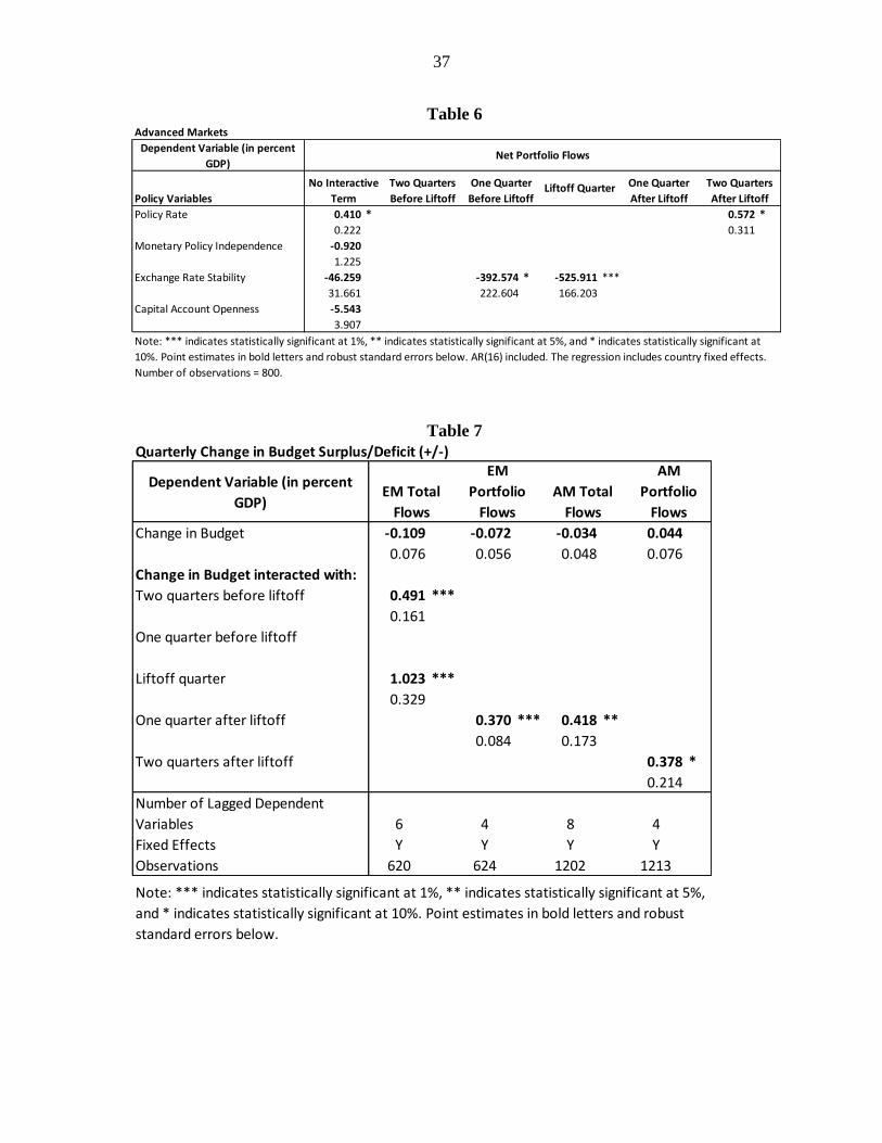
37

Table 6

Table 7

Advanced Markets

Dependent Variable (in percent

GDP)

Policy Variables

Policy Rate 0.410 * 0.572 *

0.222 0.311

Monetary Policy Independence -0.920

1.225

Exchange Rate Stability -46.259 -392.574 * -525.911 ***

31.661 222.604 166.203

Capital Account Openness -5.543

3.907

Note: *** indicates statistically significant at 1%, ** indicates statistically significant at 5%, and * indicates statistically significant at

10%. Point estimates in bold letters and robust standard errors below. AR(16) included. The regression includes country fixed effects.

Number of observations = 800.

Net Portfolio Flows

No Interactive

Term

Two Quarters

Before Liftoff

One Quarter

Before LiftoffLiftoff Quarter One Quarter

After Liftoff

Two Quarters

After Liftoff

Dependent Variable (in percent

GDP)

Change in Budget -0.109 -0.072 -0.034 0.044

0.076 0.056 0.048 0.076

Change in Budget interacted with:

Two quarters before liftoff 0.491 ***

0.161

One quarter before liftoff

Liftoff quarter 1.023 ***

0.329

One quarter after liftoff 0.370 *** 0.418 **

0.084 0.173

Two quarters after liftoff 0.378 *

0.214

Number of Lagged Dependent

Variables 6 4 8 4

Fixed Effects Y Y Y Y

Observations 620 624 1202 1213

Note: *** indicates statistically significant at 1%, ** indicates statistically significant at 5%,

and * indicates statistically significant at 10%. Point estimates in bold letters and robust

standard errors below.

EM Total

Flows

EM

Portfolio

Flows

AM Total

Flows

Quarterly Change in Budget Surplus/Deficit (+/-)AM

Portfolio

Flows

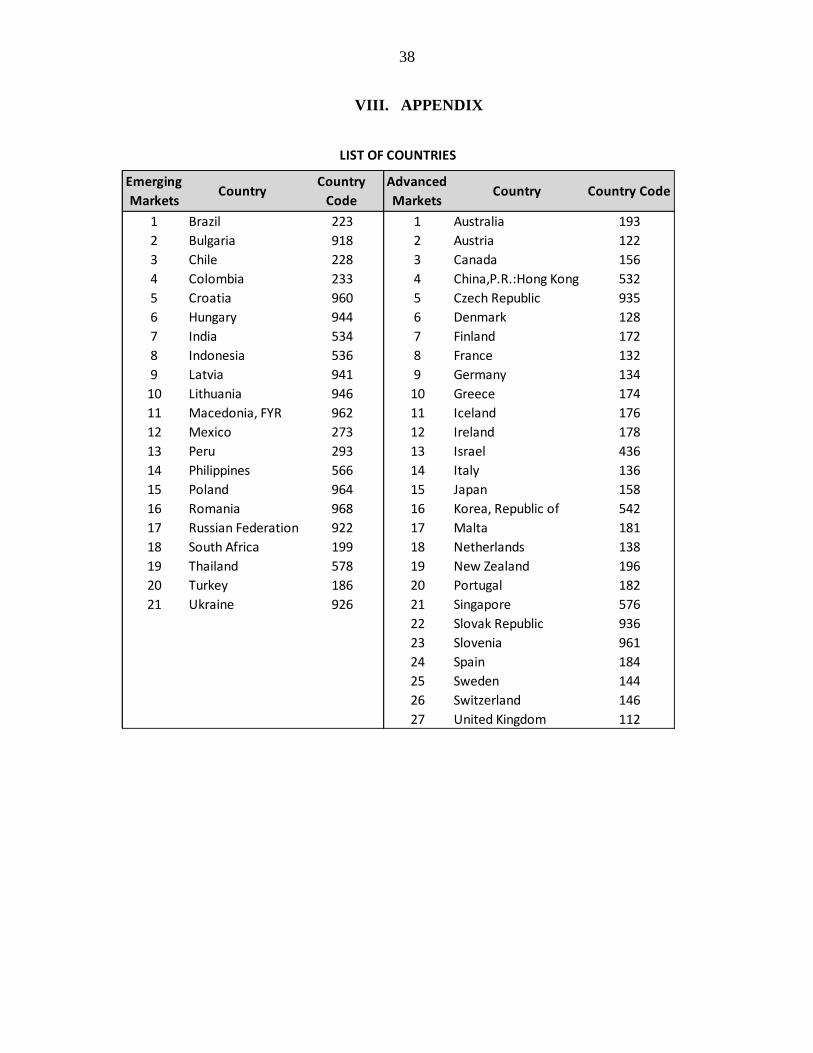
38

VIII. APPENDIX

Emerging

MarketsCountry

Country

Code

Advanced

MarketsCountry Country Code

1 Brazil 223 1 Australia 193

2 Bulgaria 918 2 Austria 122

3 Chile 228 3 Canada 156

4 Colombia 233 4 China,P.R.:Hong Kong 532

5 Croatia 960 5 Czech Republic 935

6 Hungary 944 6 Denmark 128

7 India 534 7 Finland 172

8 Indonesia 536 8 France 132

9 Latvia 941 9 Germany 134

10 Lithuania 946 10 Greece 174

11 Macedonia, FYR 962 11 Iceland 176

12 Mexico 273 12 Ireland 178

13 Peru 293 13 Israel 436

14 Philippines 566 14 Italy 136

15 Poland 964 15 Japan 158

16 Romania 968 16 Korea, Republic of 542

17 Russian Federation 922 17 Malta 181

18 South Africa 199 18 Netherlands 138

19 Thailand 578 19 New Zealand 196

20 Turkey 186 20 Portugal 182

21 Ukraine 926 21 Singapore 576

22 Slovak Republic 936

23 Slovenia 961

24 Spain 184

25 Sweden 144

26 Switzerland 146

27 United Kingdom 112

LIST OF COUNTRIES

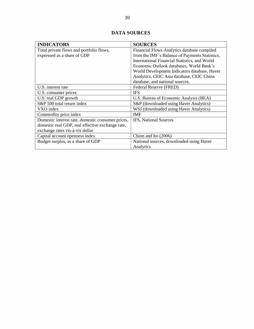
39

DATA SOURCES

INDICATORS SOURCES Total private flows and portfolio flows,

expressed as a share of GDP

Financial Flows Analytics database compiled

from the IMF’s Balance of Payments Statistics,

International Financial Statistics, and World

Economic Outlook databases, World Bank’s

World Development Indicators database, Haver

Analytics, CEIC Asia database, CEIC China

database, and national sources.

U.S. interest rate Federal Reserve (FRED)

U.S. consumer prices IFS

U.S. real GDP growth U.S. Bureau of Economic Analysis (BEA)

S&P 500 total return index S&P (downloaded using Haver Analytics)

VXO index WSJ (downloaded using Haver Analytics)

Commodity price index IMF

Domestic interest rate, domestic consumer prices,

domestic real GDP, real effective exchange rate,

exchange rates vis-à-vis dollar

IFS, National Sources

Capital account openness index Chinn and Ito (2006)

Budget surplus, as a share of GDP National sources, downloaded using Haver

Analytics