IEOR E4707: Financial Engineering: Continuous-Time Models ...janroman.dhis.org/finance/Equity/BlackScholesCtsTime.pdf · IEOR E4707: Financial Engineering: Continuous-Time Models

IEOR E4707: Financial Engineering: Continuous-Time Models Fall 2009c© 2009 by Martin Haugh

Black-Scholes and the Volatility Surface

When we studied discrete-time models we used martingale pricing to derive the Black-Scholes formula forEuropean options. It was clear, however, that we could also have used a replicating strategy argument to derivethe formula. In this part of the course, we will use the replicating strategy argument in continuous time toderive the Black-Scholes partial differential equation. We will use this PDE and the Feynman-Kac equation todemonstrate that the price we obtain from the replicating strategy argument is consistent with martingalepricing.

We will also discuss the weaknesses of the Black-Scholes model, i.e. geometric Brownian motion, and this leadsus naturally to the concept of the volatility surface which we will describe in some detail. We will also derive andstudy the Black-Scholes Greeks and discuss how they are used in practice to hedge option portfolios. We willalso derive Black’s formula which emphasizes the role of the forward when pricing European options. Finally, wewill discuss the pricing of other derivative securities and which securities can be priced uniquely given thevolatility surface. Change of numeraire / measure methods will also be demonstrated to price exchange options.

1 The Black-Scholes PDE

We now derive the Black-Scholes PDE for a call-option on a non-dividend paying stock with strike K andmaturity T . We assume that the stock price follows a geometric Brownian motion so that

dSt = µSt dt + σSt dWt (1)

where Wt is a standard Brownian motion. We also assume that interest rates are constant so that $1 invested inthe cash account at time 0 will be worth Bt := $ exp(rt) at time t. We will denote by C(S, t) the value of thecall option at time t. By Ito’s lemma we know that

dC(S, t) =(µSt

∂C

∂S+∂C

∂t+

12σ2S2 ∂

2C

∂S2

)dt + σSt

∂C

∂SdWt (2)

Let us now consider a self-financing trading strategy where at each time t we hold xt units of the cash accountand yt units of the stock. Then Pt, the time t value of this strategy satisfies

Pt = xtBt + ytSt. (3)

We will choose xt and yt in such a way that the strategy replicates the value of the option. The self-financingassumption implies that

dPt = xt dBt + yt dSt (4)= rxtBt dt+ yt (µSt dt + σSt dBt)= (rXtBt + ytµSt) dt + ytσSt dWt. (5)

Note that (4) is consistent with our earlier definition1 of self-financing. In particular, any gains or losses on theportfolio are due entirely to gains or losses in the underlying securities, i.e. the cash-account and stock, and notdue to changes in the holdings xt and yt.

1It is also worth pointing out that the mathematical definition of self-financing is obtained by applying Ito’s Lemma to (3)and setting the result equal to the right-hand-side of (4).

Black-Scholes and the Volatility Surface 2

Returning to our derivation, we can equate terms in (2) with the corresponding terms in (5) to obtain

yt =∂C

∂S(6)

rxtBt =∂C

∂t+

12σ2S2 ∂

2C

∂S2. (7)

If we set C0 = P0, the initial value of our self-financing strategy, then it must be the case that Ct = Pt for all tsince C and P have the same dynamics. This is true by construction after we equated terms in (2) with thecorresponding terms in (5). Substituting (6) and (7) into (3) we obtain

rSt∂C

∂S+

∂C

∂t+

12σ2S2 ∂

2C

∂S2− rC = 0, (8)

the Black-Scholes PDE. In order to solve (8) boundary conditions must also be provided. In the case of ourcall option those conditions are: C(S, T ) = max(S −K, 0), C(0, t) = 0 for all t and C(S, t)→ S as S →∞.

The solution to (8) in the case of a call option is

C(S, t) = StΦ(d1) − e−r(T−t)KΦ(d2) (9)

where d1 =log(St

K

)+ (r + σ2/2)(T − t)σ√T − t

and d2 = d1 − σ√T − t

and Φ(·) is the CDF of the standard normal distribution. One way to confirm (9) is to compute the variouspartial derivatives, then substitute them into (8) and check that (8) holds. The price of a European put-optioncan also now be easily computed from put-call parity and (9).

The most interesting feature of the Black-Scholes PDE (8) is that µ does not appear2 anywhere. Note that theBlack-Scholes PDE would also hold if we had assumed that µ = r. However, if µ = r then investors would notdemand a premium for holding the stock. Since this would generally only hold if investors were risk-neutral, thismethod of derivatives pricing came to be known as risk-neutral pricing.

2 Martingale Pricing

We can easily see that the Black-Scholes PDE in (8) is consistent with martingale pricing. Martingale pricingtheory states that deflated security prices are martingales. If we deflate by the cash account, then the deflatedstock price process, Yt say, satisfies Yt := St/Bt. Then Ito’s Lemma and Girsanov’s Theorem imply

dYt = (µ− r)Yt dt + σYt dWt

= (µ− r)Yt dt + σYt (dWQt − ηt dt)= (µ− r − σηt)Yt dt + σYt dW

Qt .

where Q denotes a new probability measure and WQt is a Q-Brownian motion. But we know from martingalepricing that if Q is an equivalent martingale measure then it must be the case that Yt is a martingale. This thenimplies that ηt = (µ− r)/σ for all t. It also implies that the dynamics of St satisfy

dSt = µSt dt + σSt dWt

= rSt dt + σSt dWQt . (10)

Using (10), we can now derive (9) using martingale pricing. In particular, we have

C(St, t) = EQt[e−r(T−t) max(ST −K, 0)

](11)

2The discrete-time counterpart to this observation was when we observed that the true probabilities of up-moves and down-moves did not have an impact on option prices.


whereST = Ste

(r−σ2/2)(T−t)+σWQT

is log-normally distributed. While the calculations are a little tedious, it is straightforward to solve (11) andobtain (9) as the solution.

Dividends

If we assume that the stock pays a continuous dividend yield of q, i.e. the dividend paid over the interval(t, t+ dt] equals qStdt, then the dynamics of the stock price satisfy

dSt = (r − q)St dt + σSt dWQt . (12)

In this case the total gain process, i.e. the capital gain or loss from holding the security plus accumulateddividends, is a Q-martingale. The call option price is still given by (11) but now with

ST = Ste(r−q−σ2/2)(T−t)+σWQ

T .

In this case the call option price is given by

C(S, t) = e−q(T−t)StΦ(d1) − e−r(T−t)KΦ(d2) (13)

where d1 =log(St

K

)+ (r − q + σ2/2)(T − t)

σ√T − t

and d2 = d1 − σ√T − t.

Exercise 1 Follow the argument of the previous section to derive the Black-Scholes PDE when the stock paysa continuous dividend yield of q.

Feynman-Kac

We have already seen that the Black-Scholes formula can be derived from either the martingale pricing approachor the replicating strategy / risk neutral PDE approach. In fact we can go directly from the Black-Scholes PDEto the martingale pricing equation of (11) using the Feynman-Kac formula.

Exercise 2 Derive the same PDE as in Exercise 1 but this time by using (12) and applying the Feynman-Kacformula to an analogous expression to (11).

While the original derivation of the Black-Scholes formula was based on the PDE approach, the martingalepricing approach is more general and often more amenable to computation. For example, numerical methods forsolving PDEs are usually too slow if the number of dimensions are greater3 than three. Monte-Carlo methodscan be used to evaluate (11) regardless of the number of state variables, however, as long as we can simulatefrom the relevant probability distributions. The martingale pricing approach can also be used for problems thatare non-Markovian. This is not the case for the PDE approach.

The Black-Scholes Model is Complete

It is worth mentioning that the Black-Scholes model is a complete model and so every derivative security isattainable or replicable. In particular, this means that every security can be priced uniquely. Completenessfollows from the fact that the EMM in (10) is unique: the only possible choice for ηt was ηt = (µ− r)/σ.

3The Black-Scholes PDE is only two-dimensional with state variable t and S. The Black-Scholes PDE is therefore easy tosolve numerically.


3 The Volatility Surface

The Black-Scholes model is an elegant model but it does not perform very well in practice. For example, it iswell known that stock prices jump on occasions and do not always move in the smooth manner predicted by theGBM motion model. Stock prices also tend to have fatter tails than those predicted by GBM. Finally, if theBlack-Scholes model were correct then we should have a flat implied volatility surface. The volatility surface is afunction of strike, K, and time-to-maturity, T , and is defined implicitly

C(S, 0) := BS (S, T, r, q,K, σ(K,T )) (14)

where C(S,K, T ) denotes the current market price of a call option with time-to-maturity T and strike K, andBS(·) is the Black-Scholes formula for pricing a call option. In other words, σ(K,T ) is the volatility that, whensubstituted into the Black-Scholes formula, gives the market price, C(S,K, T ). Because the Black-Scholesformula is continuous and increasing in σ, there will always4 be a unique solution, σ(K,T ). If the Black-Scholesmodel were correct then the volatility surface would be flat with σ(K,T ) = σ for all K and T . In practice,however, not only is the volatility surface not flat but it actually varies, often significantly, with time.

Figure 1: The Volatility Surface

In Figure 1 above we see a snapshot of the5 volatility surface for the Eurostoxx 50 index on November 28th,2007. The principal features of the volatility surface is that options with lower strikes tend to have higherimplied volatilities. For a given maturity, T , this feature is typically referred to as the volatility skew or smile.For a given strike, K, the implied volatility can be either increasing or decreasing with time-to-maturity. Ingeneral, however, σ(K,T ) tends to converge to a constant as T →∞. For T small, however, we often observean inverted volatility surface with short-term options having much higher volatilities than longer-term options.This is particularly true in times of market stress.

It is worth pointing out that different implementations6 of Black-Scholes will result in different implied volatilitysurfaces. If the implementations are correct, however, then we would expect the volatility surfaces to be very

4Assuming there is no arbitrage in the market-place.5Note that by put-call parity the implied volatility σ(K,T ) for a given European call option will be also be the implied

volatility for a European put option of the same strike and maturity. Hence we can talk about “the” implied volatility surface.6For example different methods of handling dividends would result in different implementations.


similar in shape. Single-stock options are generally American and in this case, put and call options will typicallygive rise to different surfaces. Note that put-call parity does not apply for American options.

Clearly then the Black-Scholes model is far from accurate and market participants are well aware of this.However, the language of Black-Scholes is pervasive. Every trading desk computes the Black-Scholes impliedvolatility surface and the Greeks they compute and use are Black-Scholes Greeks.

Arbitrage Constraints on the Volatility Surface

The shape of the implied volatility surface is constrained by the absence of arbitrage. In particular:

1. We must have σ(K,T ) ≥ 0 for all strikes K and expirations T .

2. At any given maturity, T , the skew cannot be too steep. Otherwise butterfly arbitrages will exist.

3. Likewise the term structure of implied volatility cannot be too inverted. Otherwise calendar spreadarbitrages will exist.

In practice the implied volatility surface will not violate any of these restrictions as otherwise there would be anarbitrage in the market. These restrictions can be difficult to enforce, however, when we are “bumping” or“stressing” the volatility surface, a task that is commonly performed for risk management purposes.

Why is there a Skew?

For stocks and stock indices the shape of the volatility surface is always changing. There is generally a skew,however, so that for any fixed maturity, T , the implied volatility decreases with the strike, K. It is mostpronounced at shorter expirations. There are several explanations for the skew:

1. Stocks do not follow GBM with a fixed volatility. Markets often jump and jumps to the downside tend tobe larger and more frequent than jumps to the upside.

2. Risk aversion: as markets go down, fear sets in and volatility goes up.

3. Supply and demand. Investors like to protect their portfolio by purchasing out-of-the-money puts. This isanother form of risk aversion.

4. The total value of company assets, i.e. debt + equity, is a more natural candidate to follow GBM. If so,then equity volatility should increase as the equity value decreases. This is known as the leverage effect.(See below for further explanation.)

Interestingly, there was little or no skew before the Wall street crash of 1987. So it appears to be the case thatit took the market the best part of two decades before it understood that it was pricing options incorrectly.

The Leverage Effect

Let V , E and D denote the total value of a company, the company’s equity and the company’s debt,respectively. Then the fundamental accounting equations states that

V = D + E. (15)

Equation (15) is the basis for the classical structural models that are used to price risky debt and credit defaultswaps. Merton (1970’s) recognized that the equity value could be viewed as the value of a call option on V withstrike equal to D.

Let ∆V , ∆E and ∆D be the change in values of V , E and D, respectively. ThenV + ∆V = (E + ∆E) + (D + ∆D) so that

V + ∆VV

=E + ∆E

V+D + ∆D

V

=E

V

(E + ∆E

E

)+D

V

(D + ∆D

D

)(16)


If the equity component is substantial so that the debt is not too risky, then (16) implies

σV ≈E

VσE

where σV and σE are the firm value and equity volatilities, respectively. We therefore have

σE ≈V

EσV . (17)

Example 1 (The Leverage Effect)

Suppose, for example, that V = 1, E = .5 and σV = 20%. Then (17) implies σE ≈ 40%. Suppose σV remainsunchanged but that over time the firm loses 20% of its value. Almost all of this loss is borne by equity so thatnow (17) implies σE ≈ 53%. σE has therefore increased despite the fact that σV has remained constant. This isdue to the leverage effect which helps explain the presence of skew in equity option markets.

What the Volatility Surface Tells Us

To be clear, we continue to assume that the volatility surface has been constructed from European option prices.Consider a butterfly strategy centered at K where you are:

1. long a call option with strike K −∆K

2. long a call with strike K + ∆K

3. short 2 call options with strike K

The value of the butterfly, B0, at time t = 0, satisfies

B0 = C(K −∆K,T )− 2C(K,T ) + C(K + ∆K,T )≈ e−rT Prob(K −∆K ≤ ST ≤ K + ∆K)×∆K/2≈ e−rT f(K,T )× 2∆K ×∆K/2= e−rT f(K,T )× (∆K)2

where f(K,T ) is the probability density function (PDF) of ST evaluated at K. We therefore have

f(K,T ) ≈ erTC(K −∆K,T )− 2C(K,T ) + C(K + ∆K,T )

(∆K)2. (18)

Letting ∆K → 0 in (18), we obtain

f(K,T ) = erT∂2C

∂K2.

The volatility surface therefore gives the marginal risk-neutral distribution of the stock price, ST , for any time,T . It tells us nothing about the joint distribution of the stock price at multiple times, T1, . . . , Tn.

This should not be surprising since the volatility surface is constructed from European option prices and thelatter only depend on the marginal distributions of ST .

Example 2 (Same marginals, different joint distributions)

Suppose there are 2 stocks, A and B, and that they are both initially priced at $1. There are two time periods,T1 and T2. The stock prices for t = T1 and t = T2 satisfy

S(A)t = eZ

(A)t

S(B)t = eZ

(B)t .


Suppose now that Z(A)T1

and Z(A)T2

are independent N(0, 1) random variables. Suppose also that Z(B)T1

= Z(A)T1

and thatZ

(B)T2

= αZ(A)T1

+√

1− α2Z(A)T2

.

Then each Z(A)t and Z

(B)t has an N(0, 1) distribution and so each stock has the same log-normal marginal

distribution at times T1 and T2. It therefore follows that options on A and B with the same strike and maturitymust have the same price.

But now consider an at-the-money (ATM) knockout put option with strike = 1, barrier at 1.1 and expiration atT2. The payoff function is then given by

Payoff = max (1− ST2 , 0) 1{St≤1.1 for all t: 0≤t≤T}.

Question: Would the knockout option on A have the same price as the knockout on B?

Question: How does your answer depend on α?

Question: What does this say about the ability of the volatility surface to price barrier options?

4 The Greeks

We now turn to the sensitivities of the option prices to the various parameters. These sensitivities, or theGreeks are usually computed using the Black-Scholes formula, despite the fact that the Black-Scholes model isknown to be a poor approximation to reality. But first we return to put-call parity.

Put-Call Parity

Consider a European call option and a European put option, respectively, each with the same strike, K, andmaturity T . Assuming a continuous dividend yield, q, then put-call parity states

e−rT K + Call Price = e−qT S + Put Price. (19)

This of course follows from a simple arbitrage argument and the fact that both sides of (19) equal max(ST ,K)at time T . Put-call parity is useful for calculating Greeks. For example7, it implies that Vega(Call) = Vega(Put)and that Gamma(Call) = Gamma(Put). It is also extremely useful for calibrating dividends andconstructing the volatility surface.

The Greeks

The principal Greeks for European call options are described below. The Greeks for put options can becalculated in the same manner or via put-call parity.

Definition: The delta of an option is the sensitivity of the option price to a change in the price of theunderlying security.

The delta of a European call option satisfies

delta =∂C

∂S= e−qT Φ(d1).

This is the usual delta corresponding to a volatility surface that is sticky-by-strike. It assumes that as theunderlying security moves, the volatility of the option does not move. If the volatility of the option did movethen the delta would have an additional term of the form vega× ∂σ(K,T )/∂S. In this case we would say thatthe volatility surface was sticky-by-delta. Equity markets typically use the sticky-by-strike approach whencomputing deltas. Foreign exchange markets, on the other hand, tend to use the sticky-by-delta approach.Similar comments apply to gamma as defined below.

7See below for definitions of vega and gamma.


(a) Delta for European Call and Put Options (b) Delta for Call Options as Time-To-Maturity Varies

Figure 2: Delta for European Options

By put-call parity, we have deltaput = deltacall − e−qT . Figure 2(a) shows the delta for a call and put option,respectively, as a function of the underlying stock price. In Figure 2(b) we show the delta for a call option as afunction of the underlying stock price for three different times-to-maturity. It was assumed r = q = 0. What isthe strike K? Note that the delta becomes steeper around K when time-to-maturity decreases. Note also thatdelta = Φ(d1) = Prob(option expires in the money). (This is only approximately true when r and q non-zero.)

Figure 3: Delta for European Call Options as a Function of Time-To-Maturity

In Figure 3 we show the delta of a call option as a function of time-to-maturity for three options of differentmoney-ness. Are there any surprises here? What would the corresponding plot for put options look like?


Definition: The gamma of an option is the sensitivity of the option’s delta to a change in the price of theunderlying security.

The gamma of a call option satisfies

gamma =∂2C

∂S2= e−qT

φ(d1)σS√T

where φ(·) is the standard normal PDF.

(a) Gamma as a Function of Stock Price (b) Gamma as a Function of Time-to-Maturity

Figure 4: Gamma for European Options

In Figure 4(a) we show the gamma of a European option as a function of stock price for three differenttime-to-maturities. Note that by put-call parity, the gamma for European call and put options with the samestrike are equal. Gamma is always positive due to option convexity. Traders who are long gamma can makemoney by gamma scalping. Gamma scalping is the process of regularly re-balancing your options portfolio to bedelta-neutral. However, you must pay for this long gamma position up front with the option premium. In Figure4(b), we display gamma as a function of time-to-maturity. Can you explain the behavior of the three curves inFigure 4(b)?

Definition: The vega of an option is the sensitivity of the option price to a change in volatility.

The vega of a call option satisfies

vega =∂C

∂σ= e−qTS

√T φ(d1).

In Figure 5(b) we plot vega as a function of the underlying stock price. We assumed K = 100 and thatr = q = 0. Note again that by put-call parity, the vega of a call option equals the vega of a put option with thesame strike. Why does vega increase with time-to-maturity? For a given time-to-maturity, why is vega peakednear the strike? Turning to Figure 5(b), note that the vega decreases to 0 as time-to-maturity goes to 0. This isconsistent with Figure 5(a). It is also clear from the expression for vega.

Question: Is there any “inconsistency” to talk about vega when we use the Black-Scholes model?

Definition: The theta of an option is the sensitivity of the option price to a negative change in


(a) Vega as a Function of Stock Price (b) Vega as a Function of Time-to-Maturity

Figure 5: Vega for European Options

time-to-maturity.

The theta of a call option satisfies

theta = −∂C∂T

= −e−qTSφ(d1)σ

2√T

+ qe−qTSN(d1) − rKe−rTN(d2).

(a) Theta as a Function of Stock Price (b) Theta as a Function of Time-to-Maturity

Figure 6: Theta for European Options

In Figure 6(a) we plot theta for three call options of different money-ness as a function of the underlying stockprice. We have assumed that r = q = 0%. Note that the call option’s theta is always negative. Can you explainwhy this is the case? Why does theta become more negatively peaked as time-to-maturity decreases to 0?

In Figure 6(b) we again plot theta for three call options of different money-ness, but this time as a function oftime-to-maturity. Note that the ATM option has the most negative theta and this gets more negative astime-to-maturity goes to 0. Can you explain why?


Options Can Have Positive Theta: In Figure 7 we plot theta for three put options of different money-nessas a function of time-to-maturity. We assume here that q = 0 and r = 10%. Note that theta can be positive forin-the-money put options. Why? We can also obtain positive theta for call options when q is large. In typicalscenarios, however, theta for both call and put options will be negative.

Figure 7: Positive Theta is Possible

The Relationship between Delta, Theta and Gamma

Recall that the Black-Scholes PDE states that any derivative security with price Pt must satisfy

∂P

∂t+ (r − q)S ∂P

∂S+

12σ2S2 ∂

2P

∂S2= rP. (20)

Writing θ, δ and Γ for theta, delta and gamma, we obtain

θ + (r − q)Sδ +12σ2S2Γ = rP. (21)

Equation (21) holds in general for any portfolio of securities. If the portfolio in question is delta-hedged so thatthe portfolio δ = 0 then we obtain

θ +12σ2S2Γ = rP (22)

It is clear from (22) that any gain from gamma is offset by losses due to theta. This of course assumes that thecorrect implied volatility is assumed in the Black-Scholes model. Since we know that the Black-Scholes model iswrong, this observation should only be used to help your intuition and not taken as a “fact”.

Delta-Gamma-Vega Approximations to Option Prices

A simple application of Taylor’s Theorem says

C(S + ∆S, σ + ∆σ) ≈ C(S, σ) + ∆S∂C

∂S+

12

(∆S)2 ∂2C

∂S2+ ∆σ

∂C

∂σ

= C(S, σ) + ∆S × δ +12

(∆S)2 × Γ + ∆σ × vega.

where C(S, σ) is the price of a derivative security as a function8 of the current stock price, S, and the impliedvolatility, σ. We therefore obtain

P&L = δ∆S +Γ2

(∆S)2 + vega ∆σ

8The price may also depend on other parameters, in particular time-to-maturity, but we suppress that dependence here.


= delta P&L + gamma P&L + vega P&L

When ∆σ = 0, we obtain the well-known delta-gamma approximation. This approximation is often used, forexample,in historical Value-at-Risk (VaR) calculations for portfolios that include options. We can also write

P&L = δS

(∆SS

)+

ΓS2

2

(∆SS

)2

+ vega ∆σ

= ESP× Return + $ Gamma× Return2 + vega ∆σ

where ESP denotes the equivalent stock position or “dollar” delta.

5 Delta Hedging

In the Black-Scholes model with GBM, an option can be replicated exactly by delta-hedging the option. Infact the Black-Scholes PDE we derived earlier was obtained by a delta-hedging / replication argument. The ideabehind delta-hedging is to re-balance the portfolio of the option and stock continuously so that you always havea new delta of zero. Of course it is not practical in to hedge continuously and so instead we hedge periodically.Periodic or discrete hedging then results in some replication error. Consider Figure 8 below which displays ascreen-shot of an Excel spreadsheet that was used to simulate a delta-hedging strategy.

Figure 8: Delta-Hedging in Excel

Mechanics of the Excel spreadsheet

In every period, the portfolio is re-balanced so that it is delta-neutral. This is done by using the delta of theoptions portfolio to determine the total stock position. This stock position is funded through borrowing at therisk-free rate and it accrues dividends according to the dividend yield. The timing of the cash-flows is ignoredwhen calculating the hedging P&L.

Stock prices are simulated assuming St ∼ GBM(µ, σ) so that

St+∆t = Ste(µ−σ2/2)∆t+σ

√∆tZ


where Z ∼ N(0, 1). Note the option implied volatility, σimp, need not equal σ which in turn need not equal the

realized volatility. This has interesting implications for the trading P&L and many questions arise.

Question: If you sell options, what typically happens the total P&L if σ < σimp?

Question: If you sell options, what typically happens the total P&L if σ > σimp?

Question: If σ = σimp what typically happens the total P&L as the number of re-balances increases?

Some Answers to Delta-Hedging Questions

Recall that the price of an option increases as the volatility increases. Therefore if realized volatility is higherthan expected, i.e. the level at which it was sold, we expect to lose money on average when we delta-hedge anoption that we sold. Similarly, we expect to make money when we delta-hedge if the realized volatility is lowerthan the level at which it was sold.

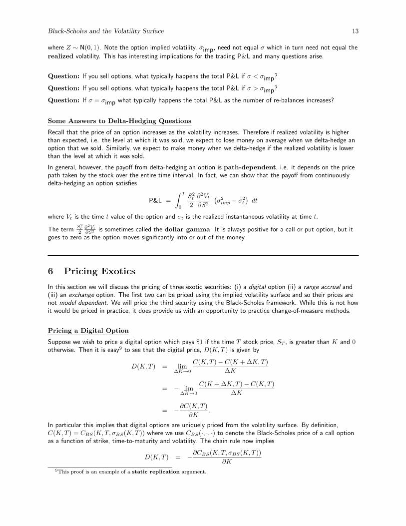
In general, however, the payoff from delta-hedging an option is path-dependent, i.e. it depends on the pricepath taken by the stock over the entire time interval. In fact, we can show that the payoff from continuouslydelta-hedging an option satisfies

P&L =∫ T

0

S2t

2∂2Vt∂S2

(σ2imp − σ2

t

)dt

where Vt is the time t value of the option and σt is the realized instantaneous volatility at time t.

The termS2

t

2∂2Vt

∂S2 is sometimes called the dollar gamma. It is always positive for a call or put option, but itgoes to zero as the option moves significantly into or out of the money.

6 Pricing Exotics

In this section we will discuss the pricing of three exotic securities: (i) a digital option (ii) a range accrual and(iii) an exchange option. The first two can be priced using the implied volatility surface and so their prices arenot model dependent. We will price the third security using the Black-Scholes framework. While this is not howit would be priced in practice, it does provide us with an opportunity to practice change-of-measure methods.

Pricing a Digital Option

Suppose we wish to price a digital option which pays $1 if the time T stock price, ST , is greater than K and 0otherwise. Then it is easy9 to see that the digital price, D(K,T ) is given by

D(K,T ) = lim∆K→0

C(K,T )− C(K + ∆K,T )∆K

= − lim∆K→0

C(K + ∆K,T )− C(K,T )∆K

= −∂C(K,T )∂K

.

In particular this implies that digital options are uniquely priced from the volatility surface. By definition,C(K,T ) = CBS(K,T, σBS(K,T )) where we use CBS(·, ·, ·) to denote the Black-Scholes price of a call optionas a function of strike, time-to-maturity and volatility. The chain rule now implies

D(K,T ) = −∂CBS(K,T, σBS(K,T ))∂K

9This proof is an example of a static replication argument.


= −∂CBS∂K

− ∂CBS∂σBS

∂σBS∂K

= −∂CBS∂K

− vega× skew.

Example 3 (Pricing a digital) Suppose r = q = 0, T = 1 year, S0 = 100 and K = 100 so the digital isat-the-money. Suppose also that the skew is 2.5% per 10% change in strike and σatm = 25%. Then

D(100, 1) = Φ(−σatm

2

)− S0 φ

(σatm2

)× −.025

.1S0

= Φ(−σatm

2

)+ .25 φ

(σatm2

)≈ .45 + .25× .4= .55

Therefore the digital price = 55% of notional when priced correctly. If we ignored the skew and just theBlack-Scholes price using the ATM implied volatility, the price would have been 45% of notional which issignificantly less than the correct price.

Exercise 3 Why does the skew make the digital more expensive in the example above?

Pricing a Range Accrual

Consider now a 3-month range accrual on the Nikkei 225 index with range 13, 000 to 14, 000. After 3 monthsthe product pays X% of notional where

X = % of days over the 3 months that index is inside the range

e.g. If the notional is $10M and the index is inside the range 70% of the time, then the payoff is $7M .

Question: Is it possible to calculate the price of this range accrual using the volatility surface?

Hint: Consider a portfolio consisting of a pair of digital’s for each date between now and the expiration.

Pricing an Exchange Option

Suppose now that there are two non-dividend-paying securities with dynamics given by

dYt = µyYt dt + σyYt dW(y)t

dXt = µxXt dt + σxXt dW(x)t

so that each security follows a GBM. We also assume dW(x)t × dW (y)

t = ρ dt so that the two security returnshave an instantaneous correlation of ρ.

Let Zt := Yt/Xt. Then Ito’s Lemma (check!) implies

dZtZt

=(µy − µx − ρσxσy + σ2

x

)dt + σydW

(y)t − σxdW

(x)t . (23)

The instantaneous variance of dZ/Z is given by(dZtZt

)2

=(σydW

(y)t − σxdW

(x)t

)2

=(σ2x + σ2

y − 2ρσxσy)dt


Now define a new process, Wt as

dWt =σyσdW

(y)t − σx

σdW

(x)t

where σ2 :=(σ2x + σ2

y − 2ρσxσy). Then Wt is clearly a continuous martingale. Moreover,

(dWt)2 =

(σy dW

(y)t − σx dW

(x)t

σ

)2

= dt.

Hence by Levy’s Theorem, Wt is a Brownian motion and so Zt is a GBM. Using (23) we can write its dynamicsas

dZtZt

=(µy − µx − ρσxσy + σ2

x

)dt + σdWt. (24)

Consider now an exchange option expiring at time T where the payoff is given by

Exchange Option Payoff = max (0, YT −XT ) .

We could use martingale pricing to compute this directly and explicitly solve

P0 = EQ0[e−rT max (0, YT −XT )

]for the price of the option. This involves solving a two-dimensional integral with the bivariate normaldistribution which is possible but somewhat tedious.

Instead, however, we could price the option by using asset Xt as our numeraire. Let Qx be the probabilitymeasure associated with this new numeraire. Then martingale pricing implies

P0

X0= EQx

0

[max (0, YT −XT )

XT

]= EQx

0 [max (0, ZT − 1)] . (25)

Equation (24) gives the dynamics of Zt under our original probability measure (whichever one it was), but weneed to know its dynamics under the probability measure Qx. But this is easy. We know from Girsanov’sTheorem that only the drift of Zt will change so that the volatility will remain unchanged. We also know thatZt must be a martingale and so under Qx this drift must be zero.

But then the right-hand side of (25) is simply the Black-Scholes option price where we set the risk-free rate tozero, the volatility to σ and the strike to 1.

Exercise 4 If asset X pays a continuous dividend yield of qx then show that only the strike in (25) needs to bechanged.

Exercise 5 If asset Y pays a continuous dividend yield of qy then show that (25) is still valid but that now wemust assume Zt pays the same dividend yield.

Pricing Other Exotics

Perhaps the two most commonly traded exotic derivatives are barrier options and variance-swaps. In fact at thisstage these securities are viewed as more semi-exotic than exotic. As suggested by Example 2, the price of abarrier option cannot be priced using the volatility surface as the latter only defines the marginal distributions ofthe stock prices. While we could use Black-Scholes and GBM with some constant volatility to determine a price,it is well known that this leads to very inaccurate pricing. Moreover, a rule employed to determine the constantvolatility might well lead to arbitrage opportunities for other market participants.

It is generally believed that variance swaps can be priced uniquely from the volatility surface. However, this isonly true for variance-swaps with maturities that are less than two or three years. For maturities beyond that, itis probably necessary to include stochastic interest rates and dividends in order to price variance swapsaccurately. Variance-swaps will be studied in detail in the assignments.


7 Dividends, the Forward and Black’s Model

Let C = C(S,K, r, q, σ, T − t) be the price of a call option on a stock. Then the Black-Scholes model says

C = Se−q(T−t)Φ(d1)−Ke−r(T−t)Φ(d2)

where

d1 =log(S/K) + (r − q + σ2/2)(T − t)

σ√T − t

,

d2 = d1 − σ√T − t. Let F := Se(r−q)(T−t) so that F is the time t forward price for delivery of the stock at

time T . Then we can write

C = Fe−r(T−t)N(d1)−Ke−r(T−t)N(d2) (26)= e−r(T−t) × Expected-Payoff-of-the-Option

where

d1 =log(F/K) + (T − t)σ2/2

σ√T − t

,

d2 = d1 − σ√T − t.

Note that the option price now only depends on F,K, r, σ and T − t. In fact we can write the call price as

C = Black(F,K, r, σ, T − t).

where the function Black(·) is defined implicitly by (26). When we write option prices in terms of the forwardand not the spot price, the resulting formula is often called Black’s formula. It emphasizes the importance of theforward price in establishing the price of the option. The spot price is only relevant in so far as it influences theforward price.

Dividends and Option Pricing

As we have seen, the Black-Scholes formula easily accommodates a continuous dividend yield. In practice,however, dividends are discrete. In order to handle discrete dividends we could convert them into dividend yieldsbut this can create problems. For example, as an ex-dividend date approaches, the dividend yield can growarbitrarily high. We would also need a different dividend yield for each option maturity. A particularly importantproblem is that delta and the other Greeks can become distorted when we replace discrete dividends with acontinuous dividend yield.

Example 4 (Discrete dividends)

Consider a deep in-the-money call option with expiration 1 week from now, a current stock price = $100 and a$5 dividend going ex-dividend during the week. Then

Black-Scholes delta = e−qT Φ(d1)≈ e−qT

= e−(.05×52)/52

= 95.12%

But what do you think the real delta is?

Using a continuous dividend yield can also create major problems when pricing American options. Consider, forexample, an American call option with expiration T on a stock that goes ex-dividend on date tdiv < T . This is


the only dividend that the stock pays before the option maturity. We know the option should only ever beexercised at either expiration or immediately before tdiv. However, if we use a continuous dividend yield, thepricing algorithm will never “see” this ex-dividend date and so it will never exercise early, even when it is optimalto do so.

There are many possible solutions to this problem of handling discrete dividends. A common solution is to takeX0 = S0 − PV(Dividends) as the “basic” security where

PV(Dividends) = present value of dividends going ex-dividend between now and option expiration.

This works fine for European options (recall that what matters is the forward). For American options, we could,for example, build a binomial lattice for Xt. Then at each date in the lattice, we can determine the stock priceand account properly for the discrete dividends, determining correctly whether it is optimal to early exercise ornot. In fact this was the subject of a question in an earlier assignment.

8 Extensions of Black-Scholes

The Black-Scholes model is easily applied to other securities. In addition to options on stocks and indices, thesesecurities include currency options, options on some commodities and options on index, stock and currencyfutures. Of course, in all of these cases it is well understood that the model has many weaknesses. As a result,the model has been extended in many ways. These extensions include jump-diffusion models, stochasticvolatility models, local volatility models, regime-switching models, garch models and others.

One of the principal uses of the Black-Scholes framework is that is often used to quote derivatives prices viaimplied volatilities. This is true even for securities where the GBM model is clearly inappropriate. Such securitiesinclude, for example, caplets and swaptions in the fixed income markets, CDS options in credit markets andoptions on variance-swaps in equity markets.

Documents

IEOR E4707: Financial Engineering: Continuous-Time Models ...janroman.dhis.org/finance/Equity/BlackScholesCtsTime.pdf · IEOR E4707: Financial Engineering: Continuous-Time Models