IEEE TRANSACTIONS ON SYSTEMS, MAN, AND …suban/papers/30smca01-shrt.pdf · (e-mail: [email protected]; [email protected]). ... we assume orthographic projection. The

IEEE TRANSACTIONS ON SYSTEMS, MAN, AND CYBERNETICS—PART A: SYSTEMS AND HUMANS, VOL. 30, NO. 1, JANUARY 2000 67

Correspondence________________________________________________________________________

Isolated 3-D Object Recognition through Next ViewPlanning

Sumantra Dutta Roy, Santanu Chaudhury, and Subhashis Banerjee

Abstract—In many cases, a single view of an object may not contain suf-ficient features to recognize it unambiguously. This paper presents a newon-line recognition scheme based on next view planning for the identifica-tion of an isolated three-dimensional (3-D) object using simple features. Thescheme uses a probabilistic reasoning framework for recognition and plan-ning. Our knowledge representation scheme encodes feature based infor-mation about objects as well as the uncertainty in the recognition process.This is used both in the probability calculations as well as in planning thenext view. Results clearly demonstrate the effectiveness of our strategy fora reasonably complex experimental set.

Index Terms—Active vision, reactive planning, 3-D object recognition.

I. INTRODUCTION

In this paper, we present a new on-line scheme for the recognitionof an isolated three-dimensional (3-D) object using reactive next viewplanning. A hierarchical knowledge representation scheme facilitatesrecognition and the planning process. The planning process utilizesthe current observation and past history for identifying a sequence ofmoves to disambiguate between similar objects.

Most model-based object recognition systems consider the problemof recognizing objects from the image of a single view [1]–[4]. How-ever, a single view may not contain sufficient features to recognizethe object unambiguously. In fact, two objects may have all views incommon with respect to a given feature set, and may be distinguishedonly through a sequence of views. Further, in recognizing 3-D objectsfrom a single view, recognition systems often use complex feature sets[2]. In many cases, it may be possible to achieve the same, incurring lesserror and smaller processing cost using a simpler feature set and suit-ably planning multiple observations. A simple feature set is applicablefor a larger class of objects than a model base specific complex featureset. Model base-specific complex features such as 3-D invariants havebeen proposed only for special cases so far (e.g., [3]). The purpose ofthis paper is to investigate the use of suitably planned multiple viewsand two-dimensional (2-D) invariants for 3-D object recognition.

A. Relation with Other Work

With an active sensor, object recognition involves identification of aview of an object and if necessary, planning further views. Tarabaniset al. [5] survey the field of sensor planning for vision tasks. We cancompare various active 3-D object recognition systems on the basis ofthe following four issues.

1) Nature of the Next View Planning Strategy:The system shouldplan moves with maximum ability to discriminate between views

Manuscript received October 23, 1997; revised May 5, 1998.S. Dutta Roy and S. Banerjee are with the Department of Computer Sci-

ence and Engineering, Indian Institute of Technology, New Delhi-110 016, India(e-mail: [email protected]; [email protected]).

S. Chaudhury is with the Department of Electrical Engineering, Indian Insti-tute of Technology, New Delhi 110 016, India.

Publisher Item Identifier S 1083-4427(00)01177-2.

common to more than one object in the model base. The cost in-curred in this process should also be minimal. The system should,preferably be on-line and reactive—the past and present inputsshould guide the planning mechanism at each stage.

While the scheme of Maver and Bajcsy [6] is on-line, that ofGremban and Ikeuchi [7] is not. Due to the combinatorial natureof the problem, an off-line approach may not always be feasible.

2) Uncertainty Handling Capability of the Hypothesis GenerationMechanism:The occlusion-based next view planning approachof Maver and Bajcsy [6], as well as that of Gremban and Ikeuchi[7] are essentially deterministic. A probabilistic strategy canmake the system more robust and resistant to errors compared toa deterministic one. Dickinsonet al. [8] use Bayesian methodsto handle uncertainty, while Hutchinson and Kak [9] use theDempster–Shafer theory.

3) Efficient Representation of Domain Knowledge:The knowledgerepresentation scheme should support an efficient mechanismto generate hypotheses on the basis of the evidence received. Itshould also play a role in optimally planning the next view.

Dickinsonet al. [8] use a hierarchical representation schemebased on volumetric primitives, which are associated with a highfeature extraction cost. Due to the non-hierarchical nature ofHutchinson and Kak’s system [9], many redundant hypothesesare proposed, which have to be later removed through consis-tency checks.

4) Speed and Efficiency of Algorithms for Both Hypothesis Gen-eration and Next View Planning:It is desirable to have algo-rithms with low order polynomial-time complexity to generatehypotheses accurately and fast. The next view planning strategyacts on the basis of these hypotheses.

In Hutchinson and Kak’s system [9], although the poly-nomial-time formulation overcomes the exponential timecomplexity associated with assigning beliefs to all possiblehypotheses, their system still has the overhead of intersectioncomputation in creating common frames of discernment. Con-sistency checks have to be used to remove the many redundanthypotheses produced earlier. Though Dickinsonet al. [8] useBayes nets for hypothesis generation, their system incurs theoverhead of tracking the region of interest through successiveframes.

The next view planning strategy that this paper presents is reactiveand on-line—the evidence obtained from each view is used in the hy-pothesis generation and the planning process. Our probabilistic hypoth-esis generation mechanism can handle cases of feature detection errors.We use a hierarchical knowledge representation scheme which not onlyensures a low-order polynomial-time complexity of the hypothesis gen-eration process, but also plays an important role in planning the nextview. The hierarchy itself enforces different constraints to prune theset of possible hypotheses. The scheme is independent of the type offeatures used, unlike that of [8]. We present results of over 100 exper-iments with our recognition scheme on two sets of models. Extensiveexperimentation shows the effectiveness of our proposed strategy ofusing simple features and multiple views for recognizing complex 3-Dshapes.

The organization of the rest of the paper is as follows: Section IIpresents our knowledge representation scheme. We discuss hypothesisgeneration for class and object recognition in Section III. Section IV

1083-4427/00$10.00 © 2000 IEEE

68 IEEE TRANSACTIONS ON SYSTEMS, MAN, AND CYBERNETICS—PART A: SYSTEMS AND HUMANS, VOL. 30, NO. 1, JANUARY 2000

describes our algorithm for planning the next view. In Section V wedemonstrate the working of our system on two sets of objects. We sum-marize the salient features of our scheme and discuss areas for furtherwork in Section VI.

II. THE KNOWLEDGE REPRESENTATIONSCHEME

A view of a 3-D object is characterized by a set of features. With re-spect to a particular feature set and over a particular range of viewingangles, a view of a 3-D object is independent of the viewpoint. Koen-derink and van Doorn [10] define aspects as topologically equivalentclasses of object appearances. Ikeuchiet al.generalize this definition:object appearances may be grouped into equivalence classes with re-spect to a feature set. These equivalence classes are aspects [11]. In thiscontext, we define the following terms:

Class A: Class (or, aspect-class) is a set of aspects, equiva-lent with respect to a feature set.

Feature-Class: A feature-class is a set of equivalent aspects de-fined for oneparticular feature.

Fig. 1 shows a simple example of an object with its associated aspectsand classes. The locus of view-directions is one-dimensional (1-D) andwe assume orthographic projection. The basis of the different classes isthe number of horizontal lines(h) and vertical lines(v) in a particularview of the object. Thus, a class may be represented ashhvi. Thereare six aspects of the object shown, belonging to three classes. In thisexample, for simplicity we assume only one feature detector so thateach feature-class is also a class.

We propose a new knowledge representation scheme encoding do-main knowledge about the object, relations between different aspects,and the correspondence of these aspects with feature detectors. Fig. 2illustrates an example of this scheme. We use this knowledge represen-tation scheme both in belief updating as well as in next view planning.Sections III andIV discuss these topics, respectively. The representa-tion scheme consists of two parts.

1) The Feature-Dependence Subnet:In the feature-dependencesubnet

• F represents the complete set of featuresfFjg used forcharacterizing views.

• A feature nodeFj is associated with feature-classesfjk.Factors such as noise and nonadaptive thresholds can introduceerrors in the feature detection process. Letpjlk represent theprobability that the feature-class present isfjl, given that the de-tector for featureFj detects it to befjk. We definepjlk as theratio of the number of times the detector for featureFj interpretsfeature-classfjl asfjk, and the number of times the feature de-tector reports the feature-class asfjk. TheFj node stores a tableof these values for its corresponding feature detector.

• A class nodeCi stores itsa priori probability,P (Ci). Alink between classCi and feature-classfjk indicates thatfjk forms a subset of features observed inCi. This ac-counts for aPART-OFrelation between the two. Thus, aclass represents ann-vector[f1j f2j � � � fnj ]. Since aclass cannot be independent of any feature, each class hasn input edges corresponding to then features.

2 The Class-Aspect Subnet:The class-aspect subnet encodes therelationships between classes, aspects, and objects.

• O represents the set of all objectsfOig• An object nodeOi stores its probability,P (Oi).• An aspect nodeaij stores its angular extent�ij (in de-

grees), its probabilityP (aij), its parent classCj , and itsneighboring aspects.

• Aspectaij has aPART-OFrelationship with its parent ob-jectOi. Thus,3-tuplehOi; Cj ; �iki represents an aspect.

Fig. 1. Aspects and classes of an object.

Fig. 2. Example of the knowledge representation scheme.

Aspect nodeaij has exactly one link to any object(Oi)and exactly one link to its parent classCj .

III. H YPOTHESISGENERATION

The recognition system takes any arbitrary view of an object as input.Using a set of features (the feature-classes), it generates hypothesesabout the likely identity of the class. This is, in turn used for gener-ating hypotheses about the object’s identity. The interaction of the hy-pothesis generation part with the rest of the system is shown in Fig. 3.Hypothesis generation consists of two steps namely, class identifica-tion, and object identification.

A. Class Identification, Accounting for Uncertainty

Our algorithm suitably schedules feature detectors to perform prob-abilistic class identification. In what follows, we discuss its various as-pects. Fig. 4 presents the overall algorithm.

1) Ordering of Feature Detectors:A proper ordering of feature de-tectors speeds up the class recognition process. At any stage, we choosethe hitherto unused feature detector for which the feature-class corre-sponding to the most probable class has the least number of outgoingarcs, i.e., the least out-degree. This is done in order to obtain that fea-ture-class which has the largest discriminatory power in terms of thenumber of classes it could correspond to. For example, in Fig. 2 if allfeature detectors are unused andC2 has the highesta priori probability,F3 will be tried first, followed byF2 andF1, if required.


Fig. 3. Flow diagram depicting the flow of information and control in our system.

Fig. 4. Class recognition algorithm.

2) Class Probability Calculations Using the Knowledge Represen-tation Scheme:We obtain thea priori probability of classCi as

P (Ci) =p

P (Op) �q

P (apqjOp) : (1)

Here, aspectsapq belong to classCi. Let NF , NC , andNa denotethe number of feature-classes associated with feature detectorFj , thenumber of classes, and the number of aspects, respectively.P (apqjOp)is�pq=360. We can computeP (Ci) from our knowledge representationscheme by considering each aspect node belonging to an object andtesting if it has a link to nodeCi; this takesO(NC + Na) time. (TheNC term is for the initialization of class probabilities to 0.)

Let the detector for featureFj report the feature-class obtained to befjk. Given this evidence, we obtain the probability of classCi from theBayes rule

P (Cijfjk) =P (Ci) � P (fjkjCi)

m

[P (Cm) � P (fjkjCm)](2)

P (fjkjCi) is 1 for those classes which have a link from feature-classfjk. It is 0 for the rest. The computation of(2) takesO(NC) time—thisis done for each feature-class. Hence, the computation ofP (fjkjCi) forall feature-classesfjk for feature detectorFj takes timeO(NF � NC).

For an error-free situation,P (Cijfjk) is P 0(Ci), the a posterioriprobability of classCi. However, due to errors possible in the featuredetection process, a degree of uncertainty is associated with the evi-dence. The value ofP 0(Ci) is, then

P 0(Ci) =l

P (Cijfjl) � pjlk (3)

wherefjl’s are feature-classes associated with featureFj . Accordingto our knowledge representation scheme, only one feature-class underfeatureFj , sayfjr has a link to classCi. The summation reduces to oneterm,P (Cijfjr) � pjrk. Thus, our knowledge representation schemealso enable recovery from feature detection errors.

B. Object Identification

Based on the outcome of the class recognition scheme, we estimatethe object probabilities as follows. Initially, we calculate thea prioriprobability of each aspect as

P (aj k ) = P (Oj ) � P (aj k jOj ): (4)


(a) (b)

Fig. 5. (a) The notation used (Section IV) and (b) a case when our algorithmis not guaranteed to succeed (Section IV-A).

If there areN objects in the model base, we initializeP (Oj ) to1=Nbefore the first observation. For the first observation,P (aj k jOjp) is�j k =360. A priori aspect probability calculations takeO(Na) time.

For any subsequent observation, we haveto account for the move-ment in the probability calculations. For example, a particular move-ment may preclude the occurrence of some aspects for a given classobserved. The value ofP (aj k jOj ) is given by

P (aj k jOj ) = �j k =360 (5)

where�j k (�j k 2 [0; �j k ]) represents the angular range pos-sible within aspectaj k for the move(s) taken to reach this posi-tion. Due to the movement made, we could have observed onlym(0 � m � r) aspects out of a total ofr aspects belonging to classCi.

Experiments with Model Base I

Let the class recognition phase report the observed class to beCi.Let us assume thatCi could have come from aspectsaj k , aj k ,� � � ; aj k , where allj1; j2; � � � ; jm are not necessarily different.We obtain thea posterioriprobability of aspectaj k given this evi-dence using the Bayes rule

P (aj k jCi) =P (aj k ) � P (Cijaj k )

m

p=1

[P (aj k ) � P (Cijaj k )]

(6)

P (Cijaj k ) is1 for aspects with a link to classCi, 0 otherwise. Finally,we obtain thea posterioriprobability

P (Oj ) =l

P (aj k jCi) (7)

where aspectsaj k belong to classCi.If the probability of some object is above a predetermined threshold

(experimentally determined, e.g., 0.87 for Model Base I), the algorithmreports a success, and stops. If not, it means that the view of the objectis not sufficient to identify the object unambiguously. We have to takethe next view.

In our hierarchical scheme, the link conditional probabilities (rep-resenting relations between nodes) themselves enforce consistencychecks at each level of evidence. The feature evidence is progressivelyrefined as it passes through different levels in the hierarchy, leading tosimpler evidence propagation and less computational cost. This is anadvantage of our scheme over that proposed in [9].

IV. NEXT VIEW PLANNING

The class observed in the class recognition phase could have comefrom many aspects in the model base, each with its own range of po-sitions within the aspect. Due to this ambiguity, one has to search for

Fig. 6. Partially constructed search tree.

Fig. 7. Object recognition algorithm.

the best move to discern between these competing aspects subject tomemory and processing limitations, if any. The parameters describedabove characterize the state of the system. The planning process aimsto determine a move from the current step, which would uniquely iden-tify the given object. We pose the planning problem as that of a forwardsearch in the state space which takes us to a state in which the aspectlist corresponding to the class observed has exactly one node. We use asearch tree for this purpose. A search tree node represents the followinginformation: [Fig. 5(a)] the unique class observed for the angular move-ment made so far, the aspects possible for this angle-class pair, and foreach aspect, the range of positions possible within it( sij � eij).

sij

and eij denote the two positions within aspectaij where the currentviewpoint can be, as a result of the movement made thus far. Here, sij � eij ; and sij ,

eij 2 [0; �ij ], where�ij is the angular extent of

aspectaij . A leaf node is one which has either one aspect associatedwith it or corresponds to a total angular movement of 360� or morefrom the root node.

Fig. 6 shows an example of a partially constructed search tree. Froma view point, we categorize possible moves as follows.


Fig. 8. Model Base I: The objects (from left) areO ,O ,O ,O ,O , O , O , andO , respectively.

(a)

(b)

(c)

(d)

Fig. 9. Some experiments with Model Base I: initial classh232i. The objects areO [(a) and (c)], andO [(b) and (d)], respectively. (a)h232i ! h231(221)i ! h232i ! h221i ! h232i. (b) h232i ! h221i ! h221i ! h221i. (c) h232i ! h232i ! h221i. (d)h232i ! h221i ! h221i ! h221i. The numbers above the arrows denote the number of turntable steps. A negative sign indicates a clockwise movement.(The figure in parentheses shows an example of recovery from feature detection errors.)

Primary Move: A primary move represents a move from an aspectby �, the minimum angle needed to move out of it.

Auxiliary Move: An auxiliary move represents a move from an as-pect by an angle corresponding to the primary move of another com-peting aspect.

Let�cij and�a

ij represent the minimum angles necessary to move outof the current assumed aspect in the clockwise and counterclockwisedirections, respectively. Three cases are possible.

1) Type I Move: �cij and�a

ij both take us out of the current aspectto a single aspect in each of the two directions—aip andaiq,

respectively. We construct search tree nodes corresponding toboth moves.

2) Type II Move: Exactly one out of�cij and�a

ij takes us to a singleaspectaip. For the other direction, the aspect we would reachdepends upon the initial position(2

sij ;

eij ]) in the current as-

pect. We construct a search tree node corresponding to the formermove.

3) Type III Move: Whether we move in the clockwise or the coun-terclockwise direction, the aspect reached depends on the initialposition in the current aspect. We choose the move which leads


(a)

(b)

(c)

(d)

(e)

(f)

Fig. 10. Some experiments with Model Base I: initial classh221i. Primary moves alone (a)O : h221i ! h221i ! h423i. (b)O : h221i !

h221i ! h221i ! h221i ! h221i. (c)O : h221i ! h232i ! h232i. Primary and auxiliary moves (d)O : h221i ! h221i ! h423i. (e)O : h221i ! h221i ! h322i. (f) O : h221i ! h232i ! h232i ! h221i ! h232i. The numbers above the arrows denote the number ofturntable steps. A negative sign indicates a clockwise movement.

us to the side with the largest angular range possible in any reach-able aspect.

We expand a nonleaf node by generating child nodes correspondingto primary moves for all competing aspects in its aspect list. We can

also generate additional child nodes by considering auxiliary moves.We assign a code to each move, a higher code to a less preferred move.We assign a code 0 to Types I and II primary moves and 1 to Type IIauxiliary moves. Type III primary moves get a code of 2, and Type III


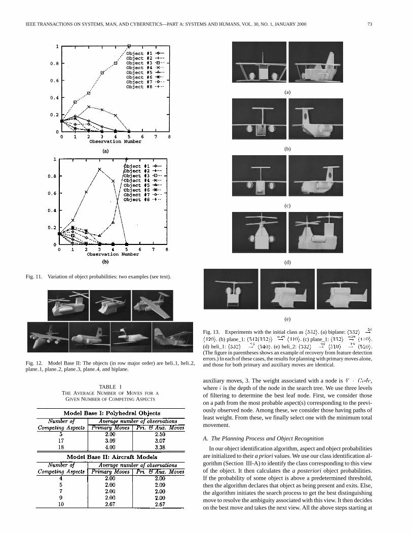
Fig. 11. Variation of object probabilities: two examples (see text).

Fig. 12. Model Base II: The objects (in row major order) are heli1, heli 2,plane1, plane2, plane3, plane4, and biplane.

TABLE ITHE AVERAGE NUMBER OF MOVES FOR A

GIVEN NUMBER OF COMPETING ASPECTS

(a)

(b)

(c)

(d)

(e)

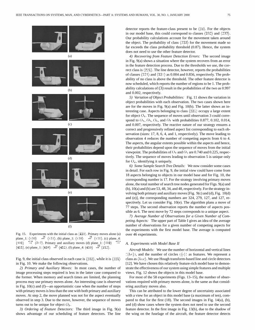
Fig. 13. Experiments with the initial class ash332i. (a) biplane:h332i !

h420i. (b) plane_1:h342(332)i ! h410i. (c) plane_1:h332i ! h410i.(d) heli_1:h332i ! h540i. (e) heli_2:h332i ! h510i ! h510i.(The figure in parentheses shows an example of recovery from feature detectionerrors.) In each of these cases, the results for planning with primary moves alone,and those for both primary and auxiliary moves are identical.

auxiliary moves, 3. The weight associated with a node is4i

� Code,wherei is the depth of the node in the search tree. We use three levelsof filtering to determine the best leaf node. First, we consider thoseon a path from the most probable aspect(s) corresponding to the previ-ously observed node. Among these, we consider those having paths ofleast weight. From these, we finally select one with the minimum totalmovement.

A. The Planning Process and Object Recognition

In our object identification algorithm, aspect and object probabilitiesare initialized to theira priori values. We use our class identification al-gorithm (Section III-A) to identify the class corresponding to this viewof the object. It then calculates thea posterioriobject probabilities.If the probability of some object is above a predetermined threshold,then the algorithm declares that object as being present and exits. Else,the algorithm initiates the search process to get the best distinguishingmove to resolve the ambiguity associated with this view. It then decideson the best move and takes the next view. All the above steps starting at


(a)

(b)

(c)

(d)

(e)

(f)

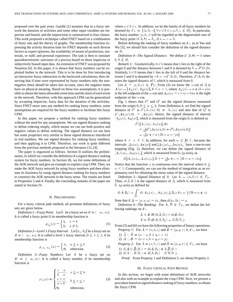
Fig. 14. Experiments with the initial class ash411i. Primary moves alone (a)plane_2:h411i ! h114i. (b) plane_2:h411i ! h114i. (c) plane_1:h411i ! h332i. Primary and auxiliary moves (d) plane_2:h411i !

h114i. (e) plane_2:h411i ! h215(214)i. (f) plane_1:h411i ! h332i.(The figure in parentheses shows an example of recovery from feature detectionerrors.)

the class identification phase are repeated. Fig. 7 presents our overallobject identification algorithm in detail. Fig. 3 shows the interaction ofthe next view planning part with the rest of the system.

Search tree node expansion is always finite due to the following rea-sons: the number of aspects is finite, and no aspect is repeated alonga search tree path. Further, even if competing objects have the sameaspects, search tree expansion stops when the total movement alonga path is 360�. Primary moves eliminate redundant image processingoperations, while auxiliary moves enable better aspect resolution. Our

planning scheme is global—its reactive nature incorporates all previousmovements and observations both in the probability calculations (Sec-tion III-B) as well as in the planning process. Our robust class recog-nition algorithm can recover from many feature detection errors at theclass recognition phase itself (Section III-A-2). If the view indeed cor-responds to the most probable aspect at a particular stage, then oursearch process using primary and auxiliary moves is guaranteed to per-form aspect resolution and uniquely identify the object in the followingstep, assuming no feature detection errors. Even if the view does notcorrespond to the most probable aspect, the list of possible aspects aview could correspond to is refined at each observation stage. The plan-ning process is initiated with the new aspect list. This illustrates the re-active nature of our planning strategy.

Assuming no feature detection errors, our algorithm is guaranteedto succeed except in three cases. The first is for objects with the sameaspect structure (i.e., the layout of classes in the aspect graph) but dif-ferent aspect angles. Further, our strategy does not handle the case whenthe aspect angles are greater than or equal to 180�. Fig. 5(b) shows anexample of the third case. Let us suppose that we have to move coun-terclockwise. Let denote the angular extent of the smallest aspectobserved so far. The current viewpoint lies in this angular range. Letaij+1 be a unique aspect for the assumed object. The counterclock-wise movement will be by an angle +!. If +! > �ij+1, we maymiss this unique aspect altogether.

B. Bounds on the Number of Observations

It is instructive to consider bounds onTavg(n), the number of ob-servations required to disambiguate between a set ofn aspects (cor-responding to the initially observed class). For a simple case to serveas a benchmark, let us assume the number of aspects reachable fromany aspect as 1, and no movement or image processing errors. We alsoassume no errors in either movement or image processing. We choosea move that partitions the initial aspect set into more than one equiva-lence class. If the size of the aspect list in one such equivalence classis j, the expected additional number of observations isTavg(j), wherej 2 [1; n). We haveTavg(n) = 1 + ( n�1

j=1Tavg(j))=(n� 1), and

Tavg(1) = 1. By induction, we can show thatTavg(n) = O(loge n).

V. RESULTS AND DISCUSSION

Our experimental setup has a camera connected to a MATROXimage processing card and a stepper motor-controlled turntable.The turntable moves by 200 steps to complete a 360� movement.We use simple and robust features with low feature extraction cost,compared to systems using complex features (e.g., [8] uses volumetricprimitives).

We have experimented extensively with two object sets as modelbases. We have chosen such objects in our model base that most of themhave more than one view in common. The list of possible aspects asso-ciated with one initial view is quite large. Our experiments have beenwith both strategies—to have primary moves alone, and both primaryand auxiliary moves for expanding the search tree node correspondingto an observation.

1) Polyhedral Objects:We use as features, the number of hori-zontal and vertical lines(hhvi), and the number of nonbackground seg-mented regions in an image(hri). We represent a class ashhvri. Weuse a Hough transform-based line detector [12]. For getting the numberof regions in the image, we perform sequential labeling (connectedcomponents: pixel labeling) [12] on a thresholded gradient image. Wehave chosen this model base so that most objects have more than oneview in common—the degree of ambiguity associated with a view isvery large. Fig. 8 shows the objects in this model base. Figs. 9 and 10show some experiments with the objects in the first model base. For


(a)

(b)

(c)

(d)

(e)

(f)

Fig. 15. Experiments with the initial class ash410i. Primary moves alone (a)plane_1:h410i ! h411i. (b) plane_1:h410i ! h411i. (c) plane_4:h410i ! h212i. Primary and auxiliary moves (d) plane_1:h410i !

h411i. (e) plane_1:h410i ! h411i. (f) plane_4:h410i ! h212i.

Fig. 9, the initial class observed in each case ish232i, while it is h221iin Fig. 10. We make the following observations.

2) Primary and Auxiliary Moves:In most cases, the number ofimage processing steps required is less in the latter case compared tothe former. When memory and search times are limited, the planningprocess may use primary moves alone. An interesting case is observedin Fig. 10(c) and (f)—an opportunistic case when the number of stepswith primary moves is less than the one with both primary and auxiliarymoves. At step 2, the move planned was not for the aspect eventuallyobserved in step 3. Due to the move, however, the sequence of movesturns out to be unique for objectO3.

3) Ordering of Feature Detectors:The third image in Fig. 9(a)shows advantage of our scheduling of feature detectors. The line

detector reports the feature-class present to beh23i. For the objectsin our model base, this could correspond to classesh232i andh233i.Our probability calculations account for the movement taken aroundthe object. The probability of classh232i for the movement made sofar exceeds the class probability threshold (0.87). Hence, the systemdoes not need to use the other feature detector.

4) Recovering from Feature Detection Errors:The second imagein Fig. 9(a) shows a situation where the system recovers from an errorin the feature detection process. Due to the thresholds we use, the cor-rect class ish221i. The line detector, however, reports the probabilitiesof classesh221i andh231i as 0.004 and 0.856, respectively. The prob-ability of no class is above the threshold. The other feature detector isnow scheduled, which reports the number of regions to be 1. The prob-ability calculations of(3) result in the probabilities of the two as 0.997and 0.002, respectively.

5) Variation of Object Probabilities:Fig. 11 shows the variation inobject probabilities with each observation. The two cases shown hereare for the moves in Fig. 9(a) and Fig. 10(b). The latter shows an in-teresting case. Aspects belonging to classh221i occupy a large extentfor objectO4. The sequence of moves until observation 3 could corre-spond toO4, O5, O6, andO7 with probabilities 0.877, 0.102, 0.014,and 0.007, respectively. The reactive nature of our strategy ensures acorrect and progressively refined aspect list corresponding to each ob-servation (sizes: 17, 8, 6, 4, and 1, respectively). The move leading toobservation 4 reduces the number of competing aspects from 6 to 4.The aspects, the angular extents possible within the aspects and hence,their probabilities depend upon the sequence of moves from the initialviewpoint. The probabilities ofO4 andO5 are 0.740 and 0.225, respec-tively. The sequence of moves leading to observation 5 is unique onlyfor O5, identifying it uniquely.

6) Some Sample Search Tree Details:We now consider some casesin detail. For each row in Fig. 9, the initial view could have come from18 aspects belonging to objects in our model base and for Fig. 10, thecorresponding number is 17. For the strategy involving primary movesalone, the total number of search tree nodes generated for Figs. 9(a) and(b), 10(a) and (b) are 53, 48, 34, and 48, respectively. For the strategy in-volving both primary and auxiliary moves [Fig. 9(c) and (d), Fig. 10(d)and (e)], the corresponding numbers are 324, 279, 127, and 127, re-spectively. Let us consider Fig. 10(e). The algorithm plans a move of77 steps. The second observation reports the number of aspects pos-sible as 6. The next move by 72 steps corresponds to a unique aspect.

7) Average Number of Observations for a Given Number of Com-peting Aspects:The upper part of Table I gives an idea of the averagenumber of observations for a given number of competing aspects forthe experiments with the first model base. The average is computedover 46 experiments.

A. Experiments with Model Base II

Aircraft Models: We use the number of horizontal and vertical lines(hhvi), and the number of circles(hci) as features. We represent aclass ashhvci. We use Hough transform-based line and circle detectors[12]. We have chosen this relatively feature-rich model base to demon-strate the effectiveness of our system using simple features and multipleviews. Fig. 12 shows the objects in this model base.

For most of the 58 experiments (Figs. 13–15), the number of obser-vations required with primary moves alone, is the same as that consid-ering auxiliary moves also.

This can be attributed to the lower degree of uncertainty associatedwith a view for an object in this model base (a maximum of ten), com-pared to that for the first (18). The second images in Fig. 14(a), (b),and (d) show cases where the system does not need to use the secondfeature detector. In the first image in Fig. 13(b), due to the shadow ofthe wing on the fuselage of the aircraft, the feature detector detects


four vertical lines instead of three, the correct number. Our recoverymechanism (Section III-A-2) corrects this error. For the experimentsshown in Fig. 14, the number of search tree nodes constructed for pri-mary moves alone is 14, whereas the corresponding number for bothprimary and auxiliary moves is 125. The corresponding numbers forthe experiments in Fig. 15 are 14 and 41, respectively.

VI. CONCLUSIONS

This paper presents an integrated approach for the recognition ofan isolated 3-D object through on-line next view planning using prob-abilistic reasoning. Our knowledge representation scheme facilitatesplanning by exploiting the relationships between features, aspects, andobject models. The recognition scheme has the ability to correctly iden-tify objects even when they have a large number of similar views. If afeature set is not rich enough to identify an object from a single view,this strategy may be used to identify it from multiple views. We demon-strate that the proposed recognition strategy works correctly even underprocessing and memory constraints due to the incremental reactiveplanning strategy. No related work has addressed this problem.

While we use simple features for the purpose of illustration, one mayuse other features such as texture, color, specularities, and reflectanceratios. Over 100 experiments demonstrate the effectiveness of usingsimple features and multiple views even on a relatively complex classof objects with a high degree of ambiguity associated with a view ofthe object. Our experiments show that one may use simple features torecognize objects with complex 3-D shapes (as in Fig. 12).

Major areas for further work include multiple object recognitionand searching for an object in a cluttered environment. This would re-quire suitably incorporating occlusion handling techniques (e.g., thosein [13]). An extension of this work would take movement errors intoaccount.

REFERENCES

[1] P. J. Besl and R. C. Jain, “Three-dimensional object recognition,”ACMComput. Surv., vol. 17, pp. 76–145, Mar. 1985.

[2] R. T. Chin and C. R. Dyer, “Model based recognition in robot vision,”ACM Comput. Surv., vol. 18, pp. 67–108, Mar. 1986.

[3] A. Zisserman, D. Forsyth, J. Mundy, C. Rothwell, J. Liu, and N. Pillow,“3-D object recognition using invariance,”Artif. Intell., vol. 78, pp.239–288, 1995.

[4] D. P. Mukherjee and D. Dutta Majumder, “On shape from symmetry,”Proc. Ind. Nat. Sci. Acad., vol. A-62, no. 5, pp. 415–428, 1996.

[5] K. A. Tarabanis, P. K. Allen, and R. Y. Tsai, “A survey of sensor planningin computer vision,”IEEE Trans. Robot. Automat., vol. 11, pp. 86–104,Feb. 1995.

[6] J. Maver and R. Bajcsy, “Occlusions as a guide for planning the nextview,” IEEE Trans. Pattern Anal. Machine Intell., vol. 15, pp. 76–145,May 1993.

[7] K. D. Gremban and K. Ikeuchi, “Planning multiple observations for ob-ject recognition,”Int. J. Comput. Vis., vol. 12, pp. 137–172, Apr. 1994.

[8] S. J. Dickinson, H. I. Christensen, J. Tsotsos, and G. Olofsson, “Ac-tive object recognition integrating attention and view point control,”Comput. Vis. Image Understand., vol. 67, pp. 239–260, Sept. 1997.

[9] S. A. Hutchinson and A. C. Kak, “Planning sensing strategies in a robotwork cell with multi-sensor capabilities,”IEEE Trans. Robot. Automat.,vol. 5, pp. 765–783, Dec. 1989.

[10] J. J. Koenderink and A. J. van Doorn, “The internal representation ofsolid shape with respect to vision,”Biol. Cybern., vol. 32, pp. 211–216,1979.

[11] K. D. Gremban and K. Ikeuchi, “Appearance-based vision and theautomatic generation of object recognition programs,” inThree-Di-mensional Object Recognition Systems, A. K. Jain and P. J. Flynn,Eds. Amsterdam, The Netherlands: Elsevier, 1993, pp. 229–258.

[12] R. M. Haralick and L. G. Shapiro,Computer and Robot Vi-sion. Reading, MA: Addison-Wesley, 1992.

[13] D. Dutta Majumder and K. S. Ray, “Recognition and position determina-tion of partially occluded object for a computer vision system,”J. IETE,vol. 37, no. 5/6, pp. 419–442, 1991.

Fuzzy Critical Path Method Based on Signed DistanceRanking of Fuzzy Numbers

Jin-Shing Yao and Feng-Tse Lin

Abstract—In this paper, we apply a signed distance ranking method forfuzzy numbers to a critical path method for activity-on-edge (AOE) net-works. We use signed distance ranking to define ordering simply, whichmeans we can use both positive and negative values to define ordering. Theprimary result obtained in this paper is the use of signed distance rankingof fuzzy numbers obtaining Properties 3 and 4. We conclude that the fuzzyAOE network is an extension of the crisp AOE network, and thus the fuzzycritical path in a fuzzy AOE network, under some conditions, is the sameas the crisp critical path in a crisp AOE network.

Index Terms—Activity-on-edge (AOE) network, critical path method,fuzzy number, signed distance ranking.

I. INTRODUCTION

Activity-on-edge (AOE) networks have proved very useful for per-formance evaluation of some types of projects. This evaluation includesdetermining certain aspects about the project, e.g., what is the leastamount of time in which the project may be completed, and which in-dividual activities should be speeded to reduce overall project length,etc. [2]. Since the activities in an AOE network can be carried out inparallel, the minimum time to complete the project is the length of thelongest path from the start of project to its finish. The longest path isthe critical path. To identify the critical path, three parameters for eachof its activities are determined:

1) earliest event time;2) latest event time;3) slack time.

The critical path is the one from the start of project to the finish ofproject where the slack times are all zeros. The purpose of the criticalpath method (CPM) is to identify critical activities on the critical pathso that resources may be concentrated on these activities in order toreduce project length time. Besides, CPM has proved very valuablein evaluating project performance and identifying bottlenecks. Thus,CPM is a vital tool for the planning and control of complex projects.

The successful implementation of CPM requires the availability ofa clear determined time duration for each activity. However, in prac-tical situations this requirement is usually hard to fulfill since many ofactivities will be executed for the first time. Hence, there is always un-certainty about the time duration of activities in the network planning,leading to the development of fuzzy critical path methods. In devel-oping the fuzzy critical path approach, several approaches have been

Manuscript received February 6, 1999; revised July 24, 1999.J.-S. Yao is with the Department of Mathematics, National Taiwan University,

Taipei, Taiwan, R.O.C.F.-T. Lin is with the Department of Applied Mathematics, Chinese Culture

University, Taipei, Taiwan, R.O.C.Publisher Item Identifier S 1083-4427(00)01180-2.

1083-4427/00$10.00 © 2000 IEEE


proposed over the past years. Gazdik [1] assumes that in a fuzzy net-work the duration of activities and some other input variables are im-precise and biased, and the imprecision is summarized to four classes.This work proposed a technique called FNET based on a combinationof fuzzy sets and the theory of graphs. The membership function ex-pressing the activity duration time for FNET depends on such diversefactors as expert opinions; the availability of means of production, ma-terials, or staff; and personal experience. The task is then to simulatequasideterministic outcomes of a process based on those imprecise orsubjectively biased input data. An extension of FNET was proposed byNasution [4]. In this paper, it is shown that fuzzy numbers can be ex-ploited further in the network. This is to be done by first introducingan interactive fuzzy subtraction in the backward calculations; then ob-serving that if time were represented by fuzzy numbers only the non-negative times should be taken into account, since the negative timeshave no physical meaning. Based on these two assumptions, it is pos-sible to obtain the latest allowable event time and the slack of each eventin the network. Therefore, with this approach CPM can be generalizedby accepting imprecise, fuzzy data for the duration of the activities.Since FNET never uses any method for ranking fuzzy numbers, someassumptions are required for the fuzzy numbers to facilitate this fuzzyCPM.

In this paper, we propose a method for ranking fuzzy numberswithout the need for any assumptions. We use signed distance rankingto define ordering simply, which means we can use both positive andnegative values to define ordering. The signed distance we use herehas some properties very similar to those signed distances introducedin real numbers. We use signed distance for ranking fuzzy numbers,and then applying it to CPM. Therefore, our work is quite differentfrom the previous methods proposed in the literature [1], [4].

The paper is organized as follows. Section II outlines the prelimi-naries, in which we consider the definition of a signed distance rankingsystem for fuzzy numbers. In Section III, we list some definitions ofthe AOE network and give an example to explain crisp CPM. Then, wemake the AOE fuzzy network by using fuzzy numbers and then elimi-nate its fuzziness by using signed distance ranking for fuzzy numbersto construct the AOE network in the fuzzy sense. The results are listedin Properties 3 and 4. Finally, the concluding remarks of the paper arestated in Section IV.

II. PRELIMINARIES

For a fuzzy critical path method, all pertinent definitions of fuzzysets are given below.

Definition 1—Fuzzy Point:Let~b1 be a fuzzy set onR = (�1;1).It is called a fuzzy point if its membership function is

�~b (x) =1; x = b

0; x 6= b:(1)

Definition 2—Level� Fuzzy Interval: Let [a�; b�] be a fuzzy set onR = (�1;1). It is called a level� fuzzy interval,0 � � � 1, if itsmembership function is

�[a ; b ](x) =�; a � x � b

0; otherwise.(2)

Definition 3—Fuzzy Numbers:Let ~A be a fuzzy set onR = (�1;1). It is called a fuzzy number, if its membershipfunction is

�~A(x) =

x� a

b� a; a � x � b

c� x

c� b; b � x � c

0; otherwise,

(3)

wherea< b< c. In addition, we let the family of all fuzzy numbers bedenoted byFN = f(a; b; c)j 8 a< b< c; a; b; c 2 Rg. In particular,the fuzzy number(a; b; c) will be regarded as the degenerated case ofthe fuzzy point(b; b; b) = ~b1, if a = c = b.

Before defining the ranking of fuzzy numbers onFN as in Yao andWu [5], we should first consider the definition of the signed distanceonR.

Definition 4—The Signed Distance:We defined�(b; 0) = b whenb, 0 2 R.

Remark 1: Geometrically,0<b means thatb lies to the right of theorigin 0 and the distance betweenb and 0 is denoted byb = d�(b; 0).Similarly, b< 0 means thatb lies to the left of 0 and the distance be-tweenb and 0 is denoted by�b = �d�(b; 0). Therefore,d�(b; 0) de-notes the signed distance ofb, which is measured from 0.

Let ~A = (a; b; c) 2 FN . From (3) we know the�-cut of ~A isA(�) = [AL(�); AR(�)], 0 � � � 1, whereAL(�) = a+(b� a)�is the left endpoint of the�-cut andAR(�) = c� (c� b)� is the rightendpoint of the�-cut.

Fig. 1 shows thatP 0 andQ0 are the signed distances measuredfrom the origin 0,0 � � � 1. From Definition 4, we find the signeddistance ofP 0 is d�(AL(�); 0) = AL(�) and also that ofQ0 isd�(AR(�); 0) = AR(�). Hence, the signed distance of interval[AL(�); AR(�)], which is measured from the origin 0, is defined as

d�([AL(�); AR(�)]; 0)

= 12 [d

�(AL(�); 0) + d�(AR(�); 0)]

= 12[a+ c+ (2b� a� c)�]

where0 � � � 1. In addition, for each� 2 [0; 1], because theintervals[AL(�); AR(�)] and[AL(�)�; AR(�)�] have a one-to-onemapping (Fig. 1), therefore, we can define the signed distance of[AL(�)�; AR(�)�], which is measured from~01 (y-axis), as

d([AL(�)�; AR(�)�]; ~01) =12[a+ c+ (2b� a� c)�]:

Notice that the function� is continuous over the interval where0 �� 1. Consequently, we can use the method of integration as an ex-planatory tool for obtaining the mean value of the signed distance.

Definition 5—Signed Distance of~A: Let ~A = (a; b; c) 2 FN .Then,d( ~A; ~01) is the signed distance of~A, which is measured from~01 (y-axis) as defined by

d( ~A; ~01) =1

0

d([AL(�)�; AR(�)�]; ~01) d� = 14(2b+ a+ c):

Note that if ~A = (a; a; a) = ~a1, thend(~a1; ~01) = a.Definition 6—The Ranking:For ~A, ~B 2 FN , we define the fol-

lowing rankings onFN~A � ~B iff d( ~A; ~01)<d( ~B; ~01)

~A � ~B iff d( ~A; ~01) = d( ~B; ~01):

From [3] and [6] we have the following properties of binary operations.Property 1: For ~A = (a; b; c) and ~B = (p; q; r) 2 FN , we have

1) ~A � ~B = (a + p; b + q; c + r)2) ~A ~B = (a � r; b � q; c � p).

Property 2: For ~A = (a; b; c) and ~B = (p; q; r) 2 FN , we have

1) d( ~A � ~B; ~01) = d( ~A; ~01) + d( ~B; ~01)2) d( ~A ~B; ~01) = d( ~A; ~01) � d( ~B; ~01).

Proof: From Property 1 and Definition 5, we obtain Property 2.

III. FUZZY CRITICAL PATH METHOD

In this section, we begin with some definitions of AOE networksand also with an example to explain the crisp CPM. Next, we present aprocedure based on signed distance ranking of fuzzy numbers, to obtainthe fuzzy CPM.


Fig. 1. The�-cut of fuzzy number~A.

Fig. 2. Crisp AOE networkN = (V;A; T ).

A. CPM in Crisp Case

An AOE network is a directed acyclic graph in which the verticesrepresent events and the edges represent project activities or tasks to beperformed on a project [2]. Formally, an AOE network is representedby N = (V;A; T ). Let V = fv1; v2; � � � ; vng be a set of verticesrepresenting a set of events, wherev1 is the start of the project,vn isits completion, andA � V �V is the set of directed edges connectingthe vertices. The tasks to be performed on the project are representedby directed edges. For each activityb 2 A, a magnitudetb 2 T isdefined, wheretb is the time required for the completion of activityb[1], [4].

Example 1: Finding a crisp critical path in an AOE network,N =(V;A; T ).

Fig. 2 is an example of an AOE network for a hypothet-ical project with seven events and ten tasks or activities. LetV = fvj = j � 1jj = 1; 2; � � � ; 7g be the set of seven events;A= f(v1; v2), (v1; v3), (v1; v4), (v2; v3), (v3; v4), (v2; v5), (v3; v6),(v4; v6), (v5; v6), (v6; v7)g be the set of ten activities; andT =ftv v , tv v , tv v , tv v , tv v , tv v , tv v , tv v , tv v , tv v gbe the number associated with each activity representing the timeneeded to perform that activity, wheretv v = t01 = 3, tv v = t02= 4, tv v = t03 = 6, etc. Thus, the activity(v1; v2) requires threedays, whereas(v1; v3) requires four days. Usually, these times areonly estimates. The critical path of this network is(v1; v2), (v2; v3),(v3; v4), (v4; v6), (v6; v7).

In an AOE network,N = (V;A; T ), whereV = fv1; v2; � � � ; vng.Let tv v be the processing time for each activity(vi; vj). We definethe earliest event time for eventvi and the latest event time for eventvjastEv andtLv , respectively. Assume that the values oftv v , tEv ,andtLv are already known. From Fig. 3 we see thattEv andtLv ,representing the earliest event time for eventvj and the latest eventtime for eventvi, satisfy the following equations:

tEv = tEv + tv v (4)

tLv = tLv � tv v : (5)

Also, letTv v be the total available time for activity(vi; vj). We obtain

Tv v = tLv � tEv : (6)

Fig. 3. Diagram of t ; t ; t ; t ; t , and T inN = (V;A; T ).

Fig. 4. A triangular fuzzy number~t .

Let Dj = fvijvi 2 V and(vi; vj) 2 Ag be a set of events obtainedfrom eventvj 2 V such that(vi; vj) 2 A andvi<vj . In Example 1,for instance, ifvj = v4(= 3) thenD4 = fvijvi 2 V and(vi; v4) 2Ag = fv1; v3g = f0; 2g. Clearly, from Fig. 3, we can obtaintEv foreventvj by using the following equations:

tEv = maxv 2D

[tEv + tv v ] and tEv = tLv = 0: (7)

Similarly, letEi = fvj jvj 2 V and(vi; vj) 2 Ag be a set of eventsobtained from eventvi 2 V , such that(vi; vj) 2 A andvi<vj . Forinstance in Example 1, ifvi = v3(= 2) thenE3 = fvj jvj 2 V and(v3; vj) 2 Ag = fv4; v6g= f3; 5g. Then, we obtaintLv for eventviby using the following equations:

tLv = minv 2E

[tLv � tv v ] and tLv = tEv : (8)

Finally, when

Tv v = tv v ; i.e., tLv = tEv + tv v (9)

we conclude that activity(vi; vj) is definitely on the critical path of thecrisp network.

B. Fuzzy CPM Based on Signed Distance Ranking of Fuzzy Numbers

As noted earlier in this section, for each activity(vi; vj), we as-sume that the values oftv v , tEv , andtLv are already known andtEv , tLv , andTv v can be obtained from (7), (8), and (6), respec-tively. However, this assumption may cause severe difficulties in prac-tice. Therefore, here we considertv v is only an estimate and is im-precise. Thus, we maketv v fuzzy by using the following triangularfuzzy number (Fig. 4)

~tv v = (tv v ��v v 1; tv v ; tv v +�v v 2);

0<�v v 1<tv v ; 0<�v v 2: (10)

By Definition 5, we haved(~tv v ; ~01) = tv v + 1

4(�v v 2��v v 1).

It is the signed distance of~tv v measured from~01. Sinced(~tv v ; ~01)= 1

4(3tv v + �v v 2) +

1

4(tv v � �v v )> 0, we conclude that

d(~tv v ; ~01) is a positive distance between~tv v and~01. In other words,the processing time is measured from the origin 0. Thus, we define


t�v v to be an estimate of the processing time for activity(vi; vj) inthe fuzzy sense, i.e.

t�

v v = d(~tv v ; ~01) = tv v + 1

4(�v v 2 ��v v 1): (11)

Remark 2: If �v v 1 = �v v 2, i.e., the triangle in Fig. 4 isan isosceles triangle, then we havet�v v = tv v . In particular, if�v v 1 = �v v 2 = 0, then the fuzzy case will become crisp.

As we mentioned above, in the crisp AOE network,N = (V;A; T ),the earliest event timetEv for eventvi, the latest event timetLvfor eventvj , and the total available timeTv v for activity (vi; vj)are directly derived from (7), (8), and (6), respectively. However,in practice, the decision-maker should realize that these time vari-ables are imprecise and consider them in a fuzzy sense. Thus, anestimate of the earliest event time for eventvi is in the interval[tEv � �EEv 1; tEv + �Ev 2], 0<�Ev 1<tEv , 0<�Ev 2,wheretEv is a known number. In considering the accuracy, we findthat when the earliest event time is exactlytEv , the error rate isdefinitely 0. Clearly, greater imprecision of time will produce largererror rates. When an estimate eventually approaches one of the twoends of the interval, i.e.,tEv ��Ev 1 or tEv +�Ev 2, the error ratebecomes largest. However, it is preferable to use the term “confidencelevel” rather than “error rate.” Thus, when the earliest event time isexactlytEv , we obtain the confidence level is 1. On the other hand,when an estimate approaches one of the two ends of the interval, theconfidence level becomes the smallest. In this section, we will usethe fuzzy number from (12) below and use the membership grade torepresent the confidence level.

Similar to the abovetv v in (10), which corresponds to the interval[tEv � �Ev 1; tEv + �Ev 2], we then define the fuzzy number oftEv as

~tEv = (tEv ��Ev 1; tEv +�Ev 2) (12)

where0<�Ev 1<tEv , 0<�Ev 2, and the parameters satisfy (15)and (23) below. We then definet�Ev to be an estimate of the earliestevent time for eventvi in the fuzzy sense, i.e.,

t�

Ev = d(~tEv ; ~01) = tEv + 1

4(�Ev 2 ��Ev 1) (>0): (13)

From (4), i.e.,tEv = tEv + tv v , we fuzzify both sides of theequation to obtain~tEv � ~tEv � ~tv v . Note that� is the ranking forFN , as defined in Definition 6. From Definitions 5 and 6, and also fromProperty 2, we haved(~tEv ; ~01) = d(~tEv � ~tv v ; ~01) = d(~tEv ; ~01)

+ d(~tv v ; ~01). From (11) and (13), we obtain the following equation:

t�

Ev = t�

Ev + t�

v v : (14)

Thus, we have

tEv + 1

4(�Ev 2 ��Ev 1)

= tEv + tv v + 1

4[�Ev 2 ��Ev 1 + (�v v 2 ��v v 1)]:

According to (4), we obtain the following condition for parameters:

�Ev 2 ��Ev 1 = (�Ev 2 ��Ev 1) + (�v v 2 ��v v 1):

(15)

Similarly, the fuzzy number oftLv is defined as

~tLv = (tLv ��Lv 1; tLv ; tLv +�Lv 2) (16)

where0<�Lv 1<tLv and0<�Lv 2, and the parameters must sat-isfy (19) and (23) below. Then, we definet�Lv to be an estimate of thelatest event time for eventvj in the fuzzy sense, i.e.

t�

Lv = d(~tLv ; ~01) = tLv + 1

4(�Lv 2 ��Lv 1): (17)

Fuzzifying both sides of (5),tLv = tLv � tv v , yields ~tLv �

~tLv ~tv v . From Definitions 5 and 6, and from Property 2, we ob-

taind(~tLv ; ~01) = d(~tLv ; ~01)� d(~tv v ; ~01). From (11) and (17) weobtain the following equation:

t�

Lv = t�

Lv � t�

v v : (18)

Then, we have

tLv + 1

4(�Lv 2 ��Lv 1)

= tLv � tv v + 1

4[(�Lv 2 ��Lv 1)

� (�v v 2 ��v v 1)]:

According to (5), we obtain the following condition for parameters

�Lv 2 ��Lv 1 = (�Lv 2 ��Lv 1)� (�v v 2 ��v v 1): (19)

The fuzzy number of the total available timetv v is defined as

~Tv v = (Tv v �$v v 1; Tv v ; Tv v +$v v 2) (20)

where0<$v v 1<Tv v and0<$v v 2, and the parameters mustsatisfy (23) and (24) below. LetT �

v v be an estimate of the total avail-able time for activity(vi; vj) in the fuzzy sense, i.e.

T�

v v = d( ~Tv v ; ~01) = Tv v + 1

4($v v 2 �$v v 1): (21)

Fuzzifying both sides of (6),Tv v = tLv � tEv , yields ~Tv v �

~tLv ~tEv . From Definitions 5 and 6, and from Property 2, we haved( ~Tv v ; ~01) = d(~tLv ; ~01) � d(~tEv ; ~01). From (13), (17), and (21)we obtain the following equation

T�

v v = t�

Lv � t�

Ev : (22)

Therefore we have

Tv v + 1

4($v v 2 �$v v 1)

= tLv � tEv + 1

4[�Lv 2 ��Lv 1 + (�Ev 2 ��Ev 1)]:

From (6), we obtain the following condition for parameters:

$v v 2 �$v v 1 = (�Lv 2 ��Lv 1)� (�Ev 2 ��Ev 1): (23)

Finally, fuzzifying both sides of (9),Tv v = tv v , yields ~Tv v �

~tv v . Similarly, we obtainT �

v v = t�v v and also have

Tv v + 1

4($v v 2 �$v v 1) = tv v + 1

4(�v v 2 ��v v 1):

SinceTv v = tv v , we obtain the condition for parameters

$v v 2 �$v v 1 = �v v 2 ��v v 1: (24)

Furthermore, from (15), (19), (23), and (24) we obtain the followingconditions for parameters,

�Lv 2 ��Lv 1 = �Ev 2 ��Ev 1

�Lv 2 ��Lv 1 = �Ev 2 ��Ev 1

and

(�Lv 2 ��Lv 1)� (�Ev 2 ��Ev 1)

= �v v 2 ��v v 1: (25)

Remark 3: Here we compare the crisp AOE network for the effortsmade by a decision-maker with the fuzzy AOE network. Consider eachactivity (vi; vj) in the crisp AOE network. The values oftv v , tEv ,and tLv are already known, however, the values oftEv , tLv , andTv v are determined according to (6)–(8). On the other hand, for eachactivity (vi; vj) in the fuzzy AOE network, the fuzzy number~tv v

in (10) must satisfy0<�v v 1<tv v and 0<�v v 2. The otherfuzzy numbers~tEv , ~tLv , and ~Tv v , as defined in (12), (16), and(20), respectively, are determined as follows. Since the values oftEv ,tEv , tLv , tLv , andTv v , as well as the values oftv v , �v v 1,and�v v 2 in (10) are already known; the decision-maker can chooseappropriate values for�Ev q, �Ev q , �Lv q , �Lv q, and$v v q ,whereq = 1; 2 to satisfy (15), (19), (23), and (24), respectively. (SeeExample 2 and Remark 4.)

While T �

v v = t�v v , i.e., t�Lv = t�Ev + t�v v , we conclude thatthe activity(vi; vj) is on the fuzzy critical path. Next, the processing


time tb(2 T ) is considered for each activityb(2 A) in the crisp AOEnetwork,N = (V;A; T ). We fuzzify tb as~tb, and then obtaining anestimate of the processing time for activityb in the fuzzy sense,t�b =d(~tb; ~01). Let T � = ft�b j8 tb 2 T; b 2 A; t�b = d(~tb; ~01g. Hence, weconstruct a fuzzy AOE network,N� = (V;A; T �). From the previousdiscussions we summarize the following property.

Property 3: Consider the fuzzy AOE network,N� = (V;A; T �).The fuzzy numbers oftv v , tEv , tLv , andTv v , are~tv v , ~tEv ,~tLv , and ~Tv v , respectively. When those fuzzy numbers satisfy (15),(19), (23), and (24), we obtain the following significant results.

1) An estimate of the processing time of activity(vi; vj) in thefuzzy sense is

t�

v v = tv v + 1

4(�v v 2 ��v v 1):

2) An estimate of the earliest event time of eventvi in the fuzzysense is

t�

Ev = tEv + 1

4(�Ev 2 ��Ev 1):

3) An estimate of the latest event time of eventvj in the fuzzy senseis

t�

Lv = tLv + 1

4(�Lv 2 ��Lv 1):

4) An estimate of the total available time of activity(vi; vj) in thefuzzy sense is

T�

v v = Tv v + 1

4($v v 2 �$v v 1):

5) t�Ev = t�Ev + t�v v ; t�Lv = t�Lv � t�v v , andT �

v v = t�Lv �t�Ev .

6) WhenT �

v v = t�v v , i.e., t�Lv = t�Ev + t�v v , the activity(vi; vj) is on the fuzzy critical path.

Now, from (7) we knowtEv + tv v � tEv , 8 vi 2 Dj , and alsoknow there is at least one equal sign which holds. When both sidesof the above equation are fuzzified, we obtain~tEv � ~tv v ~tEv ,8 vi 2 Dj , and also know there is at least one�which holds. The sym-bols� are� the ranking onFN (see Definition 6). From Definitions5 and 6 and also from Property 2, we obtain the following equationsd(~tEv ; ~01) + d(~tv v ; ~01) � d(~tEv ; ~01), 8 vi 2 Dj , and also knowthere is at least one equal sign which holds. Furthermore, from (11) and(13) we knowt�Ev + t�v v � t�Ev , 8 vi 2 Dj , and also know at leastone equal sign holds there. Hence, we obtain the following equation:

t�

Ev = maxv 2D

(t�Ev + t�

v v ): (26)

Sincet�Ev + t�v v � t�Ev , 8 vi 2 Dj , we obtain

tEv + tv v + 1

4f(�Ev 2 ��Ev 1) + (�v v 2 ��v v 1g

� tEv + 1

4(�Ev 2 ��Ev 1); 8 vi 2 Dj :

In fact, the above equation can be derived directly from (15) andtEv +tv v � tEv , 8 vi 2 Dj . Therefore, no additional conditions for pa-rameters are needed in (26).

Next, consider the equationtEv = tLv = 0. After fuzzifying bothsides of the equation, we obtain~tEv � ~tLv � ~01 andd(~tEv ; ~01) =d(~tLv ; ~01) = d(~01; ~01). Hence, we obtaint�Ev = t�Lv = 0, butit requires an additional condition,�Ev 2 = �Ev 1 = �Lv 2 =�Lv 1 = 0.

Similarly, from (8) we havetLv � tLv �tv v ,8 vj 2 Ei, and alsohave at least one equal sign which holds. We use the same procedureto fuzzify both sides of the equation, obtaining~tLv ~tLv ~tv v ,8 vj 2 Ei and also determine that at least one� holds. From Def-initions 5 and 6, and also from Property 2, we derive the equation,d(~tLv ; ~01) � d(~tLv ; ~01)�d(~tv v ; ~01),8 vj 2 Ei, where at least oneequal sign holds. Furthermore, from (11) and (17) we obtaint�Lv �

t�Lv � t�v v , 8 vj 2 Ei, where at least one equal sign holds. Thus wederive the following equation:

t�

Lv = maxv 2E

(t�Lv � t�

v v ): (27)

Similar to (26), the above equation can be derived from (19) andtLv � tLv � tv v , 8 vj 2 Ei. Therefore, no additional conditionsfor parameters are needed in (27). Finally, we consider the equationtLv = tEv . After fuzzifying the equation, we obtain~tLv � ~tEvandd(~tLv ; ~01) = d(~tEv ; ~01). Then, by (13) and (17), we obtaint�Lv = t�Ev and an additional condition for parameters:

�Lv 2 ��Lv 1 = �Ev 2 ��Ev 1: (28)

If t�Ev = t�Lv , then an estimate of the earliest event time for eventvj in the fuzzy sense is equal to an estimate of the latest event timefor eventvj in the fuzzy sense. Obviously, this indicates there is noslack time. In conclusion, we summarize the above statements in thefollowing property.

Property 4: Consider the fuzzy AOE network,N� = (V;A; T �).If �Ev 2 = �Ev 1 = �Lv 2 = �Lv 1 = 0, and�Lv 2 � �Lv 1

= �Ev 2 � �Ev 1, as well as the conditions in Property 3 hold, wesummarize the following results.

1) An estimate of the earliest event time for eventvj inthe fuzzy sense ist�Ev , which can be derived fromt�Ev = maxv 2D (t�Ev + t�v v ) andt�Ev = t�Lv = 0.

2) An estimate of the latest event time for eventvi in the fuzzy senseis t�Lv , which can be derived fromt�Lv = minv 2E (t�Lv �t�v v ) andt�Lv = t�Ev .

3) The activity(vi; vj) will on the critical path ift�Ev = t�Lv andt�Ev = t�Lv .

Proof: Equations (1) and (2) can be proved directly from (26) and(27). Sincet�Ev = t�Lv andt�Ev = t�Lv , from (5) of the Property 3,we obtaint�v v = t�Ev � t�Ev = t�Lv � t�Ev = T �v v . By (6) ofProperty 3, we have proved (3).

Example 2: Construct a fuzzy AOE network,N� = (V;A; T �),from the crisp AOE network,N = (V;A; T ), of Example 1. Let~tv v

= (2.1, 3, 3.8),~tv v = (3.5, 4, 5),~tv v = (5, 6, 7.2),~tv v = (3.2,4, 4.8),~tv v = (4, 5, 6.3),~tv v = (4.1, 5, 6.1),~tv v = (2.8, 4, 5),~tv v = (4.9, 6, 7.2),~tv v = (1.5, 2, 2.7),~tv v = (3.8, 5, 6). Aftercalculating by (1) of Property 3, we obtain the following estimates ofprocessing time in the fuzzy sense, i.e.t�v v = 2.975,t�v v = 4.125,t�v v = 6.05,t�v v = 4, t�v v = 5.075,t�v v = 5.05,t�v v = 3.95,t�v v = 6.025,t�v v = 2.05, andt�v v = 4.95. We letT � = ft�v v ,t�v v , t�v v , t�v v , t�v v , t�v v , t�v v , t�v v , t�v v , t�v v g. Hence, weconstruct a fuzzy AOE network,N� = (V;A; T �), as shown in Fig. 5.

Next, we should choose appropriate values for the parameters,i.e.,�Ev 1, �Ev 2, �Ev 1, �Ev 2, �Lv 1, �Lv 2, �Lv 1, �Lv 2,$v v 1, and$v v 2, to satisfy Properties 3 and 4. Then we calculatet�Ei andt�Ej by using (1) and (2) of Property 4 in the following table(see Remark 4).

In Table I, for example, we calculatet�E3 by using (1) of Property 4as follows. Sincej = 3, we haveDj = fij(i; j) 2 Ag = fi = 0; i =2g (see Fig. 5). From Table I, we find thatt�E0 = 0, t�E2 = 6:975,t�03 = 6:05, andt�23 = 5:075. Thus, we obtain

t�

E3 = maxft�E0 + t�

03; t�

E2 + t�

23g

= maxf0 + 6:05; 6:975 + 5:075g = 12:05:

In Table II, for example, we calculatet�L2 by using (2) of Property 4as follows. Sincei = 2, we haveEi = fjj(i; j) 2 Ag = fj = 3; j =5g (see Fig. 5). From Table II, we find thatt�L3 = 12:05, t�L5 = 18:075,t�23 = 5:075, andt�25 = 3:95. Thus, we obtaint�L2 = minft�L5 � t�25,t�L3 � t�23g = minf18:075� 3:95, 12:05� 5:075g = 6:975.

From Tables I and II, we obtain Table III. Table III shows the processof finding a fuzzy critical path inN�. According to the rule of (3) in


Fig. 5. Fuzzy AOE networkN = (V;A; T ).

TABLE ICOMPUTATION OF t , THE EARLIEST

EVENT TIME FOR EVENT i IN THE FUZZY SENSE

TABLE IICOMPUTATION OF t , THE EARLIEST EVENT TIME FOR EVENT

j IN THE FUZZY SENSE

TABLE IIIPROCESSES OFFINDING A FUZZY CRITICAL PATH IN N = (V;A; T )

Property 4, we find a critical path 0! 1! 2! 3! 5! 6 (i.e.,v1! v2 ! v3 ! v4 ! v6 ! v7). The total time of the path ist� =23:025. However, in the crisp case of Example 1, the critical path ofN = (V;A; T ) is also 0! 1! 2! 3! 5! 6, and the total timeof the path ist = 3+ 4+ 5+ 6+ 5= 23 (see Table IV).

Remark 4: An example to explain our approach for determiningthe appropriate values for those parameters to satisfy the conditionsof Properties 3 and 4. Here we only consider the activity(v5; v6).Since~tv v = (1.5, 2, 2.7), we obtain�v v 1 = 0.5 and�v v 2 =0.7 by simple subtraction. Property 3 states that the fuzzy numbers

TABLE IVCOMPUTATION OF THETOTAL TIME OF A CRITICAL PATH IN N = (V;A; T )

should satisfy (15), (19), (23), and (24). Hence,�Ev 2 � �Ev 1 =(�Ev 2��Ev 1)+0:2,�Lv 2��Lv 1 = (�Lv 2��Lv 1)�0:2,$v v 2 � $v v 1 = (�Lv 2 � �Lv 1) � (�Ev 2 � �Ev 1),$v v 2 � $v v 1 = 0:2. Sincevj = j � 1, from Table IV wehave tEv = tE4 = 8, tLv = tL4 = 16 (etc.), tEv = 18,tLv = 18, Tv v = tLv � tEv = 10, tEv = tLv = 0, andtEv = tLv = 23. Subsequently, we take the following equations�Ev 2 � �Ev 1 = �Lv 2 � �Lv 1 = 0:3, �Ev 2 � �Ev 1 =�Lv 2 ��Lv 1 = 0:1, and$v v 2 �$v v 1 = 0:2, where�Ev q ,�Ev q, �Lv q , �Lv q, $v v q , q = 1; 2, to satisfy the followingcriteria, 0<�Ev 1<tEv = 8, 0<�Ev 2, 0<�Ev 1< 18,0<�Ev 2, 0<�Lv 1< 16, 0<�Lv 2, 0<�Lv 1< 18,0<�Lv 2, 0<$v v 1<Tv v = 10, and0<$v v 2. Finally, wecould choose appropriate values for the above parameters to satisfyProperty 3. For example, we choose�Ev 2 = 0:2, �Ev 1 = 0:1,�Ev 2 = 0:5, �Ev 1 = 0:2, �Lv 2 = 0:3, �Lv 1 = 0:2,�Lv 2 = 0:4, �Lv 1 = 0:1, $v v 2 = 0:3, and$v v 1 = 0:1.Then, we obtain~tEv = (8�0:1; 8; 8+0:2),~tEv = (17:8; 18; 18:5),~tLv = (15:8;16; 16:3), ~tLv = (17:9; 18; 18:4), and~Tv v = (9:9; 10; 10:3). From (13), (17), and (21) we obtaint�Ev = t�E4 = 8:025, t�Lv = t�L4 = 16:025 (etc.),t�Ev = 18:075,t�Lv = 18:075, andT �

v v = 10:05 (= t�Lv � t�Ev ). Notice that wehave the same results here as in Table III.

IV. CONCLUDING REMARKS

This paper has presented a ranking method for fuzzy numbers ina CPM of AOE networks. The focus of the paper was to introducethe signed distance ranking of fuzzy numbers, and use them to obtainfuzzy critical paths. In Section III, we discussed fuzzy CPM based ona signed distance ranking of fuzzy numbers. When the processing timefor activity (vi; vj) in the crisp case istv v and the fuzzy numberof tv v is ~tv v = (tv v � �v v 1; tv v ; tv v + �v v 2), where0<�v v 1<tv v , and0<�v v 2, then an estimate of the processingtime in the fuzzy sense is given byt�v v = tv v + 1

4(�v v 2 �

�v v 1). Interpretation of the result is as follows, viz. Fig. 4. When�v v 1<�v v 2, the triangle goes to the right side (largertv v ), andwe obtaintv v <t�v v . Conversely, when�v v 2<�v v 1, the tri-angle goes to the left side (smallertv v ), and we obtaint�v v <tv v .However, if�v v 2 = �v v 1, then it is an isosceles triangle, so wehavetv v = t�v v . We conclude that if the following criteria a)–d)hold, the fuzzy AOE network,N� = (V;A; T �), which is defined inProperties 3 and 4, becomes the crisp AOE network,N = (V;A; T ),which is defined in Section III-A.

1) For each activity(vi; vj), if �v v 2 = �v v 1, which is definedin (11), then

t�

v v = tv v :

2) For each eventvj , if �Ev 2 = �Ev 1, as defined in (13), thent�Ev = tEv .

3) For each eventvj , if �Lv 2 = �Lv 1, as defined in (17), thent�Lv = tLv .

4) For each activity(vi; vj), if $v v 2 = $v v 1, as defined in(21), thenT �

v v = Tv v .


Consequently, we conclude that the fuzzy AOE network,N� = (V;A; T �), is an extension of the crisp AOE network,N = (V;A; T ).

In addition, we let(vj ; vj ), (vj ; vj ); � � � ; (vj ; vj ), where0<m<n, j0 = v1, and vm = vn, be the critical path in thenetwork N = (V;A; T ). The processing times for each activityon the critical path aretv v , tv v ; � � � ; tv v and theysatisfy Tv v = tv v , p = 1; 2; � � � ;m, in (9). Wemake both sides ofTv v = tv v fuzzy, thus obtaining~Tv v �

~Tv v . By Definition 6 we haved( ~Tv v ; ~01)

= d(~tv v ; ~01). Then, from (11) and (21) we obtain

T�

v v = t�

v v ; p = 1; 2; � � � ;m: (29)

Therefore,

Tv v + 1

4($v v 2 �$v v 1)

= tv v + 1

4(�v v 2 ��v v 1):

SinceTv v = tv v , we obtain the following condition forparameters

$v v 2 �$v v 1

= �v v 2 ��v v 1; p = 1; 2; � � � ;m: (30)

In summary, we conclude that if we hold (29) and (30), then by (6) ofProperty 3 and (3) of Property 4, the fuzzy critical path in a fuzzy AOEnetwork is the same as the critical path in a crisp AOE network.

REFERENCES

[1] I. Gazdik, “Fuzzy-network planning-FNET,”IEEE Trans. Rel., vol.R-32, no. 3, pp. 304–313, 1983.

[2] E. Horowitz, S. Sahni, and D. Mehta,Fundamental of Data Structuresin C++ , New York: Freeman, 1995.

[3] A. Kaufmann and M. M. Gupta,Introduction to Fuzzy Arithmetic,Theory and Applications, New York: Van Nostrand Reinhold, 1991.

[4] S. H. Nasution, “Fuzzy critical path method,”IEEE Trans. Syst., Man.,Cybern., vol. 24, pp. 48–57, Jan. 1994.

[5] J. S. Yao and K. M. Wu, “Ranking Fuzzy numbers based on decompo-sition principle and signed distance,”Fuzzy Sets Syst., to be published.

[6] H.-J. Zimmermann,Fuzzy Set Theory and Its Applications, 2nded. Boston, MA: Kluwer, 1991.

Documents

IEEE TRANSACTIONS ON SYSTEMS, MAN, AND …suban/papers/30smca01-shrt.pdf · (e-mail: [email protected]; [email protected]). ... we assume orthographic projection. The