IEEE TRANSACTIONS ON PATTERN ANALYSIS AND …jeffcohn/biblio/TPAMI2547397 FINAL.pdf · IEEE Proof Selective Transfer Machine for Personalized Facial Expression Analysis Wen-Sheng

IEEE P

roof

Selective Transfer Machine for PersonalizedFacial Expression AnalysisWen-Sheng Chu, Fernando De la Torre, and Jeffrey F. Cohn

Abstract—Automatic facial action unit (AU) and expression detection from videos is a long-standing problem. The problem is

challenging in part because classifiers must generalize to previously unknown subjects that differ markedly in behavior and facial

morphology (e.g., heavy versus delicate brows, smooth versus deeply etched wrinkles) from those on which the classifiers are trained.

While some progress has been achieved through improvements in choices of features and classifiers, the challenge occasioned by

individual differences among people remains. Person-specific classifiers would be a possible solution but for a paucity of training data.

Sufficient training data for person-specific classifiers typically is unavailable. This paper addresses the problem of how to personalize a

generic classifier without additional labels from the test subject. We propose a transductive learning method, which we refer to as a

Selective Transfer Machine (STM), to personalize a generic classifier by attenuating person-specific mismatches. STM achieves this

effect by simultaneously learning a classifier and re-weighting the training samples that are most relevant to the test subject. We

compared STM to both generic classifiers and cross-domain learning methods on four benchmarks: CK+ [44], GEMEP-FERA [67], RU-

FACS [4] and GFT [57]. STM outperformed generic classifiers in all.

Index Terms—Facial expression analysis, personalization, domain adaptation, transfer learning, support vector machine (SVM)

Ç

1 INTRODUCTION

AUTOMATIC facial AU detection confronts a number ofchallenges. These include changes in pose, scale, illumi-

nation, occlusion, and individual differences in face shape,texture, and behavior. Face shape and texture differ betweenand within sexes; they differ with ethnic and racial back-grounds, age or developmental level, exposure to the ele-ments, and in the base rates with which they occur. Forexample, some people smile frequently and broadly, whileothers smile rarely and only in a controlled manner, counter-acting the upward pull of the zygomatic major on the lip cor-ners. These and other sources of variation representconsiderable challenges for computer vision. Furthermore,there is the challenge of automatically detecting facial actionsthat require significant training and expertise in humans [67].

To address these challenges, previous work has focusedon identifying optimal feature representations and classi-fiers. Interested readers may refer to [20], [46], [49], [56] forcomprehensive reviews. While improvements have beenmade, a persistent shortcoming of existing systems is thatthey fail to generalize well to previously unseen, or new,subjects. One way to cope with this problem is to train andtest separate classifiers on each subject (i.e., person-specificclassifier). Fig. 1a shows a real example of how a simple

linear person-specific classifier can separate the positivesamples of AU12 (lip corner puller, seen in smiling) fromthe negative ones. When ample training data are available,a person-specific classifier approaches an ideal classifier, onethat best separates actions for the test subject.

A problem with person-specific classifiers is that a suffi-cient quantity of training data is usually unavailable. In partfor this reason, most approaches use training data frommul-tiple subjects in the hope to compensate for subject biases.However, as shown in Fig. 1b, when a classifier is trained onall training subjects and tested on an unknown subject, itsgeneralizability may disappoint. When a classifier is trainedand tested in this manner, we refer to it as a generic classifier.Because person-independent classifiers typically are not fea-sible, generic classifiers are commonly used.

We hypothesize that impaired generalizability occursin part because of individual differences among subjects.Fig. 2 illustrates this phenomenon on real data in a 3-Deigenspace. One can observe that if the data in Fig. 2a areinterpreted as positive and negative classes, they could bevery difficult to separate without overfitting. If the datain Fig. 2a are instead interpreted as subjects, the groupingeffect becomes clear and echoes our conjectureabout individual differences. Individual differences mayinclude sex, skin color and texture, illumination, andother ways in which people and image acquisition effectsmay vary. Our guiding hypothesis is that the person-specific bias causes standard generic classifiers to performworse on some subjects than others [28].

To mitigate the influence of individual biases, this paperexplores the idea of personalizing a generic classifier forfacial expression analysis. Given a common observationthat a test video usually comes from only a single subject,we assume the test distribution can be approximated by asubset of video frames from training subjects. The problem

� W.-S. Chu and F.D.la Torre are with the Robotics Institute, Carnegie MellonUniversity, Pittsburgh, PA 15213. E-mail: [email protected],[email protected].

� J. F. Cohn is with the Robotics Institute, Carnegie Mellon University, andwith the Department of Psychology, University of Pittsburgh, Pittsburgh,PA 15260. E-mail: [email protected].

Manuscript received 3 July 2014; revised 2 Mar. 2016; accepted 17 Mar. 2016.Date of publication 0 . 0000; date of current version 0 . 0000.Recommended for acceptance by T. Cootes.For information on obtaining reprints of this article, please send e-mail to:[email protected], and reference the Digital Object Identifier below.Digital Object Identifier no. 10.1109/TPAMI.2016.2547397

IEEE TRANSACTIONS ON PATTERN ANALYSIS AND MACHINE INTELLIGENCE, VOL. 38, NO. X, XXXXX 2016 1

0162-8828� 2016 IEEE. Personal use is permitted, but republication/redistribution requires IEEE permission.See http://www.ieee.org/publications_standards/publications/rights/index.html for more information.

mailto:

mailto:

mailto:

IEEE P

roof

of personalizing a generic classifier is then formulated astraining a classifier on selected training samples, whilereducing the discrepancy between distributions of selectedtraining samples and test ones. In this way, generic classi-fiers can adapt to unseen test subjects without test labels.We term this transductive approach a Selective TransferMachine. The major contributions of this work include:

� Based on both qualitative observations and empiricalfindings, individual differences attenuate perfor-mance of AU detection. To address this problem, weintroduce Selective Transfer Machine (STM), an unsu-pervised personalization approach that reduces mis-match between feature distributions of training andtest subjects. We propose an effective and robustprocedure to optimize STM in its primal form.

� Considering that many applications afford labeledtest data, we introduce a useful extension of STM,termed L-STM, to make use of labeled data from thetarget domain. This extension shows considerableperformance improvement in situations wherelabeled test data are available.

� To evaluate STM, we conduct comprehensive experi-ments using within-subject, cross-subject, and cross-dataset scenarios on four benchmark datasets. Wetest STM for both AU detection and detection ofholistic expressions.

� For test subjects, some training samples are moreinstrumental than others. We can identify thosetraining samples using STM. The effectiveness ofSTM scales as domain size, or the number of trainingsubjects, increases.

This paper is organized as follows. Section 2 reviewsrelated work. Sections 3–5 describe the STM model, optimi-zation algorithm, and theoretical rationale. Section 6 introdu-ces L-STM, an STM extension that utilizes labeled test data.Section 7 considers similarities and differences between STMand related methods. Section 8 evaluates STM and alterna-tives for AU and holistic expression detection. Section 9 con-cludes the paperwith remarks and futurework.

2 RELATED WORK

Our approach lies at the intersection between facial expres-sion analysis and cross-domain adaptation. Below webriefly discuss each in turn.

2.1 Facial Expression Analysis

Automatic facial expression analysis entails at least threesteps: Face tracking and registration, feature extraction,and learning classifiers. This section reviews recent advan-ces in each.

Tracking and registration. Tracking and registration ofnon-rigid facial features is a long-standing problem in com-puter vision. The goal of tracking is to detect facial land-marks (e.g., eyes) in each frame. For facial landmarkdetection, Parametrized Appearance Models (PAM) areamong the most popular methods. PAM include the Lucas-Kanade method [43], Active Appearance Models (AAM)[18], [47], Constrained Local Models (CLM) [15], and, morerecently, Zface [34] and Supervised Descent Method [74].Once facial landmarks are located, the registration stepaims to align the face image to remove 3D rigid headmotion, so features can be geometrically normalized. A sim-ilarity transformation [20], [61], [86] registers faces withrespect to an averaged face. A Delaunay triangulation canbe also applied with a backward piecewise affine warpingto extract features in areas not explicitly tracked. This two-step registration proves to preserve better shape variationin appearance than by geometric normalization alone.

Feature extraction. With advances in tracking and registra-tion, there has been a renewed emphasis on biologicallyinspired features and temporal variation. As summarized inTable 1, current approaches to feature extraction may bebroadly divided into four types: geometric, appearance, dynamic,and fusion. Geometric features contain information about theshape and locations of permanent facial features, such as eyes

Fig. 1. An illustration of the proposed Selective Transfer Machine (STM):(a) 2D PCA projection of positive (squares) and negative (circles) sam-ples for a given AU (in this case AU 12 or lip-corner raiser) for three sub-jects. An ideal classifier separates AU 12 nearly perfectly for eachsubject. (b) A generic classifier trained on all three subjects generalizespoorly to a new person (i.e., test subject) due to individual differencesbetween the 3-subject training set and the new person. STM personal-izes a generic classifier and reliably separates an AU for a new subject.

Fig. 2. Visualization of samples from the RU-FACS dataset [4] in 3Deigenspace: colors/markers indicate different (a) positive/negative clas-ses, and (b) subjects (best viewed in color).

2 IEEE TRANSACTIONS ON PATTERN ANALYSIS AND MACHINE INTELLIGENCE, VOL. 38, NO. X, XXXXX 2016

IEEE P

roof

or nose. Standard approaches rely on detecting fiducial facialpoints [45], a connected face [61], landmark coordinates [15],or face component shape parameterization [45]. Geometricfeatures have performed well for many but not all AU detec-tion tasks. They have difficulties in detecting subtle expres-sions and are highly vulnerable to registration error [16].

Appearance features, which often are biologically inspired,afford increased robustness to tracking and registration error.Appearance features represent skin texture and its permuta-tions and have been widely applied to facial expression anal-ysis. Representative methods include SIFT [86], DAISY [86],Gabor jets [4], LBP [35], [84], Bag-of-Words model [60], [61],compositional [77] and others [72].Dynamic features, a newlypopular technique, encodes temporal information during thefeature extraction stage. Examples include optical flow [32],bag of temporal words [62], volume LBP/LPQ [82], Gabormotion energy [73], and others. Fusion approaches incorpo-rate multiple features, e.g., Multiple Kernel Learning (MKL)[58], and have yet to prove superior to other approaches [67].

Classifiers. Two main trends have been pursued whendesigning classifiers for facial expression analysis, as sum-marized in Table 2. One trend, static modeling, typicallytackles the problem as discriminative classification and eval-uates each frame independently. Representative approachesinclude Neural Network [38], Adaboost [4], SVMs [45], [61],[83], andDeepNetworks [42]. Due to lack of temporal consis-tency, static models tend to produce non-smooth results. Toaddress this issue, temporal modeling, the other trend, cap-tures the temporal transition between contiguous frames.For instance, Dynamic Bayesian Network (DBN) withappearance features [65] was proposed to model AU co-occurrence. Other variants of DBN include Hidden MarkovModels [59] and Conditional Random Fields (CRF) [9], [68].As an alternative, Simon et al. [61] proposed a structural-out-put SVM that detects AUs as temporal segments. To modelrelations between segments, Rudovic et al. [52] consideredordinal information in CRF. More recently, Ding et al. [21]proposed a hybrid approach that integrates frame-based,segment-based, and transition-based tasks in a sequentialorder. Interested readers are referred to [20], [46], [49], [56],[67] for more complete surveys.

Common to all these approaches is the assumption thattraining and test data are drawn from the same distribution.However, as Fig. 2 shows, they could suffer from individualdifferences, causing poor generalizability to an unseen sub-ject. STM makes no such assumption. Instead, it seeks a per-sonalized classifier by re-weighting training samplesaccording to their distribution mismatch with test samples.Several studies merged into this direction could be found in[55], [78], [79], [80].

2.2 Cross-Domain Adaptation

Our approach is motivated by an increasing concern aboutdataset shift in the object detection literature. In real-worlddata, labels of interest could occur infrequently and featuresvary markedly between and within datasets. These factorscontribute to significant biases in object categorization [66].Saenko et al. [40], [54] proposed to reduce the discrepancybetween features by learning metric transformation. Aytarand Zisserman [2] regularized the training of a new objectclass by transferring pre-learned models. Chattopadhyayet al. [12] proposed to learn a combination of source classifiersthat matches the target labels. Because these techniques use asupervised approach in which one or more labeled instancesare required from the target domain, they are ill-suited to newdomains or subjects for which no prior knowledge is avail-able. In contrast, our approach is unsupervised and thus bet-ter geared to the generalization to newdomains or subjects.

Closer to our approach is a special case in unsuperviseddomain adaptation known as covariate shift [63]. In covariateshift, train and test domains follow different distributionsbut the label distributions remain the same.

On the other hand, Dud�ık et al. [24] infer the re-samplingweights through maximum entropy density estimationwithout target labels. Maximum Mean Discrepancy (MMD)[5] measures the discrepancy between two different distri-butions in terms of expectations of empirical samples. With-out estimating densities, Transductive SVM (T-SVM) [36]simultaneously learns a decision boundary and maximizesthe margin in the presence of unlabeled patterns. Domainadaptation SVM [6] extends T-SVM by progressively adjust-ing the discriminant function toward the target domain.SVM-KNN [81] labels a single query using an SVM trainedon its k neighborhood of the training data. Each of thesemethods uses either all or a portion of the training data.STM learns to re-weight training instances, which reducesthe influence of irrelevant data.

Considering distribution mismatch, Kernel Mean Match-ing (KMM) [31] directly infers re-sampling weights by

TABLE 1Representative Feature Extraction Methods

TABLE 2Representative Classifiers

CHU ET AL.: SELECTIVE TRANSFER MACHINE FOR PERSONALIZED FACIAL EXPRESSION ANALYSIS 3

IEEE P

roof

matching training and test distributions. Following this idea,Yamada et al. [75] estimated relative importanceweights andlearned from re-weighted training samples for 3D humanpose estimation. See [50] for further review. These methodstake a two-step approach that first estimates the samplingweights and then trains a re-weighted classifier or regressor.In contrast, STM jointly optimizes both the sampling weightsand the classifier parameters and hence preserves the dis-criminant property of the newdecision boundary.

3 SELECTIVE TRANSFER MACHINE (STM)

This section describes the proposed Selective TransferMachine (STM) for personalizing a generic classifier. Unlikeprevious cross-domain methods [2], [22], [39], [76], STMrequires no labels from a test subject. For classification pur-pose, we model STM with a Support Vector Machine (SVM)due to its popularity for AU detection [15], [35], [61].

Problem formulation. Recent research and applications inautomatic facial expression analysis consider video data,which provide awide sampling of facial appearance changes.We assume the distribution of a subject’s appearance can beestimated by certain video frames. Based on this assumption,the main idea of STM is to re-weight training samples (i.e.,frames) to form a distribution that approximates the test dis-tribution. Classifiers trained on the re-weighted training sam-ples are likely to generalize to the test subject.

Denote the training set as Dtr¼fxi; yigntri¼1; yi2fþ1;�1g(see notation1). For notational simplicity, we stack 1 in each

data vector xi to compensate for the offset, i.e., xi2Rdþ1. Weformulate STM as minimizing the objective:

gðf; sÞ ¼ minf;s

RfðDtr; sÞ þ �VsðXtr;XteÞ; (1)

where RfðDtr; sÞ is the SVM empirical risk defined on the

decision function f , and training set Dtr with each instanceweighted by selection coefficients s2Rntr . Each entry si cor-responds to a positive weight for a training sample xi.

VsðXtr;XteÞ measures training and test distribution mis-match as a function of s. The lower the value of Vs is, thecloser the training and the test distributions are. � > 0 is atradeoff between the risk and the distribution mismatch.The goal of STM is to jointly optimize the decision functionf as well as the selective coefficient s, such that the resultingclassifier can alleviate person-specific biases.

Penalized SVM. The first term in STM, RfðDtr; sÞ, is theempirical risk of a penalized SVM, where each traininginstance is weighted by its relevance to the test data. In the

following, we denote X�Xtr for notational simplicity unlessfurther referred. The linear penalized SVM has the target

decision function in the form fðxÞ¼w>x and minimizes:

RwðDtr; sÞ ¼ 1

2kwk2 þ C

Xntri¼1

siLpðyi;w>xiÞ; (2)

where Lpðy; �Þ¼maxð0; 1� y�Þp (p ¼ 1 stands for hinge lossand p ¼ 2 for quadratic loss). In general, L could be any lossfunction. The unconstrained linear SVM in (2) can be

extended to a nonlinear version by introducing a kernelmatrix Kij :¼kðxi; xjÞ, which corresponds to a kernel func-tion k induced from a nonlinear feature mapping ’ð�Þ. Usingthe representer theorem [11], the nonlinear decision func-tion can be represented fðxÞ¼Pntr

i¼1 bikðxi; xÞ, yielding thenonlinear penalized SVM:

RbbðDtr; sÞ ¼ 1

2bb>Kbbþ C

Xntri¼1

siLpðyi;k>i bbÞ; (3)

where bb2Rntr is the expansion coefficient and ki is the ithcolumn of K. Unlike most standard solvers, we train thepenalized SVM in the primal due to its simplicity and effi-ciency. Through the unconstrained primal problems, weapply Newton’s method with quadratic convergence [11].Details are given in Section 4.

Distribution mismatch. The second term in STM, VsðXtr;

XteÞ, imitates domainmismatch and aims to find a re-weight-ing function that minimizes the discrepancy between thetraining and the test distributions. In previous cross-domainlearning methods, the re-weighting function may be com-puted by separately estimating the densities and then theweights (e.g., [64]). However, this strategy could be prone toerror while taking the ratio of estimated densities [64].

To estimate the re-weighting function, here we adopt theKernel Mean Matching (KMM) [31] method, which aims toreduce the distance of empirical means between the trainingand the test distributions in the Reproducing Kernel HilbertSpace H. KMM computes the instance re-weighting si thatminimizes:

VsðXtr;XteÞ¼ 1

ntr

Xntri¼1

si’ðxtri Þ�1

nte

Xntej¼1

’ðxtej Þ��

��2

H: (4)

Let ki :¼ntrnte

Pntej¼1 kðxtri ; xtej Þ, i¼1; . . . ; ntr, capture the closeness

between a training sample and each test sample, solving s in(4) can be rewritten as a quadratic programming (QP):

mins1

2s>Ks� kk>s;

s:t: si 2 ½0; B�;Xntri¼1

si � ntr

�� ntr�;

(5)

where B defines a scope that bounds discrepancy betweenprobability distributions Ptr and Pte (B¼1;000 in our case).For B!1, one obtains an unweighted solution where allsi ¼ 1. The second constraint ensures the weighted samplesto be close to a probability distribution [31]. Observe in(5) that a larger ki leads to a larger si to minimize the objec-tive. This matches our intuition to put higher selectionweights on the training samples that are more likely toresemble the test distribution.

A major benefit from KMM is a direct importance estima-tion without estimating training and test densities. Com-pared to existing approaches, with proper tuning of kernelbandwidth, KMM shows the lowest importance estimationerror, and robustness to input dimension and the number oftraining samples [64]. Fig. 3 illustrates its effect on a syn-thetic data. As shown, KMM can estimate the ideal fittingwell, while standard Ordinary Least Square (OLS) and

1. Bold capital letters denote a matrix X; bold lower-case lettersdenote a column vector x. xi represents the ith column of the matrix X.All non-bold letters represent scalars. xj denotes the scalar in the jthelement of x. In2Rn�n is an identity matrix.


IEEE P

roof

Weighted OLS (WOLS) with training/test ratio lead to sub-optimal prediction.

4 OPTIMIZATION FOR STM

To solve Eq. (1), we adopt Alternate Convex Search [26] thatalternates between solving the decision function f and theselection coefficient s. Note that the objective in (1) is bicon-vex: Convex in f when s is fixed (f is quadratic and Lp isconvex), and convex in s when f is fixed (since K0).Under these conditions, the alternate optimization approachis guaranteed to monotonically decrease the objective func-tion. Because the function is bounded below, it will con-verge to a critical point. Algorithm 1 summarizes the STMalgorithm. Once the optimization is done, f is applied toperform the inference for test images. Below we detail thetwo steps in the alternate algorithm.

Minimizing over s. Denote the training losses as‘pi :¼Lpðyi; fðxiÞÞ, i¼1; . . . ; ntr. The optimization over s canbe rewritten into the following QP:

mins1

2s>Ksþ ðC

�‘‘p � kkÞ>s

s:t: 0 � si � B; ntrð1� �Þ �Xntri¼1

si � ntrð1þ �Þ:(6)

Since K0 by definition, (6) has only one global optimum.To make the algorithm numerically stable, we add a ridge s

on the diagonal so that K sIntr (s¼10�8 in our case).Note that the procedure here is different from the

original KMM in terms of weight refinement: In each itera-tion s will be refined through the training loss ‘‘p fromthe penalized SVM. This effect can be observed fromminimizing the second term in (6): Larger ‘‘p leads tosmaller s to keep the objective small. This effectivelyreduces the selection weights of misclassified trainingsamples. On the contrary, KMM uses no label informa-tion and thus is incapable of refining importance weights.Introducing training losses helps preserve the discrimi-nant property of the new decision boundary and henceleads to a more robust personalized classifier. From thisperspective, KMM can be treated as a special case as thefirst iteration in STM.

Algorithm 1. Selective Transfer Machine

Input: Xtr, Xte, parameters C; �Output: Inferred test labels y

$for test data

1 Initialize training loss ‘‘p 0;2 while not converged do3 Update the instance-wise re-weighting s by solving the

QP in (6);4 Update the decision function f and training loss ‘‘p by

solving the penalized SVM in (2) or (3);5 Infer test labels by y

$ fðXteÞ

Fig. 5 illustrates the iterative effect of personalizing ageneric classifier on a synthetic example. In it#1, thehyperplane estimated by KMM is unreliable due to its unsu-pervised nature. On the other hand, STM simultaneouslyconsiders the SVM loss and the similarity between trainingand test samples, and thus encourages the associated train-ing samples with small training loss to be weighted more.As can be observed, as the iterations proceed, the STM sepa-ration hyperplane moves toward the ideal hyperplane forthe target data.

Minimizing over f . Let sv indicate the index set of supportvectors, and nsv the number of support vectors. In the case

training loss ‘‘2 being quadratic, the gradient and theHessian of the linear penalized SVM in (2) can be written as:

rw ¼ wþ 2CXSI0ðX>w� yÞ; (7)

Hw ¼ Id þ 2CXSI0X>; (8)

where S¼diagðsÞ2Rntr�ntr denotes the re-weighting matrix,

y2Rntr the label vector, and I02Rntr�ntr the proximity iden-tity matrix with the first nsv diagonal elements being 1 andthe rest being 0. Similarly, the gradient with respect to theexpansion coefficient bb in (3) can be derived as:

rbb ¼ Kbbþ 2CKSI0ðKbb� yÞ; (9)

Hbb ¼ Kþ 2CKSI0K: (10)

Given the gradients and the Hessians, the penalized SVMcan be optimized in the primal using standard Newton’smethod or conjugate gradient.

Differentiable huber loss. The L1 (hinge) loss in standardSVMs are not differentiable, hampering its gradient andHessian to be explicitly expressed and computed. Instead,we use the Huber loss [11] as a differentiable surrogate, i.e.,

L1ðyi; fðxiÞÞLH yisignðfðxiÞÞð Þ. Note that any differentialconvex loss, e.g., logistic loss and exponential loss, can bedirectly incorporated. The Huber loss is defined as:

LHðaÞ ¼0 ifa > 1þ h,

ð1þh�aÞ24h if j1� aj � h,

1� a otherwise,

8<: (11)

where h is a parameter of choice. Fig. 4 shows the influnce

of h in comparison to the L1 and L2 loss. As can beobserved, LH approaches the hinge loss when h!0. Asindicated in [11], there is no clear reason to prefer the hingeloss because replacing the hinge loss with Huber loss doesnot influence much the results. With the differentiableHuber loss, the gradient and Hessian with Huber loss forthe penalized linear SVM can be obtained:

Fig. 3. Fitting a line to a quadratic function using KMM and other re-weighting methods. The larger size (more red) of training data, the moreweight KMM adopted. As can be observed, KMM puts higher weights inthe training samples closer to the test ones. Compared to standard OLSor WOLS, KMM leads to better approximation for the test data.


IEEE P

roofrw ¼ wþ C

2hXSI0 X>w� ð1þ hÞy� �� CXSI1y; (12)

Hw ¼ Id þ C

2hXSI0X>; (13)

and for the penalized nonlinear SVM:

rbb ¼ Kbbþ C

2hKSI0 Kbb� ð1þ hÞy½ � �KI1y; (14)

Hbb ¼ Kþ C

2hKSI0K; (15)

where I12Rntr�ntr denotes the proximity identity matrixwith the first nsv diagonal elements being 0, followed byn‘ (the number of points in the linear part of the Huberloss) elements of ones. With the derived gradientsand Hessians, we optimize for f using standard Newtonmethod.

5 THEORETICAL RATIONALE

This section analyzes two important properties of STM, bi-convexity and boundedness, based on the techniques devel-oped for biconvex optimization [30]. Then we justify theconvergence of the Alternate Convex Search algorithm,which we used for solving STM, in terms of both objectivevalue and optimization variables.

5.1 Properties of STM

We start by showing that STM is a biconvex problem.

Property 1. (Bi-convexity) Selective Transfer Machine in (1) is abiconvex optimization problem.

Proof. Denote the decision variable of f as w2W�Rd

and the selection coefficient s2S�Rntr , where W andS are two non-empty convex sets. Let Z �W � S bethe solution set on W � S; Zw and Zs be the subsetswhen w and s are given respectively. Because Zs isconvex for every w 2W (w and Lp are convex;si 2 ½0; B� are non-negative) and Zw is convex forevery s 2 S (Vs is QP and K 0), the solution set Zis a biconvex set. Hence STM can be rewritten in thestandard form of biconvex optimization problem [1]:minw;sfgðw; sÞ : ðw; sÞ2Zg: tu

Property 2. (Boundedness) The STM optimization problem inProblem (1) is bounded from below.

Proof. The boundedness can be observed from two aspects:(1) Rf is bounded due to the quadratic term in f andnon-negative s and Lp. (2) Vs is bounded since K is posi-tive semi-definite. tuFollowing the same proof line, the above properties can

be also shown for nonlinear STM defined with Eq. (3).

5.2 Algorithm

The following analysis mimics directly Section 4 in [30]. Wepresent the key steps for proving the convergence and referto more details on this style of proof in [30].

Alternate convex search. To solve the biconvex STM prob-lem, one approach is to exploit its convex substructure.We used the Alternate Convex Search (ACS) algorithm[71], a special case of Block-Relaxation Methods, by alter-nately solving the convex subproblems. For explanationconvenience, we recall the ACS algorithm in Algorithm 2.

Denote z ¼ ðw; sÞ as the solution variable. As men-tioned in Section 4, STM can be seen as initializing s0using KMM or a uniform vector, and then solving theclassifier w1 as an unweighed SVM. As will be discussedbelow and in Section 8.5, the permutation order does notinfluence the convergence. For Step 4, there are severalways to determine the stopping criterion. We used therelative decrease of z compared to the last iteration.Below we discuss the convergence properties in terms ofobjective value (i.e., the difference between gðztÞ andgðzt�1Þ of two consecutive iterations t and t� 1), and thevariables (i.e., the difference between zt and zt�1).

Convergence. Recall thatW and S are two non-empty sets,and Z �W � S is a biconvex set on W � S. We firstly show

Fig. 5. Comparisons of a generic SVM, a personalized STM, and an ideal classifier for synthetic data. The left-most figure shows the convergencecurve of the objective value. Figures it#1,4,8,12 with training/test accuracy (Tr% and Te%) show the corresponding hyperplanes at each iteration.Grey (shaded) dots denote training samples, and white (unshaded) dots denote test samples. Circles and squares denote two different classes.Note that it#1 indicates the results of KMM [31]. STM improves separation relative to the generic SVM as early as the 1st iteration and convergestoward the ideal hyperplane by the 12th iteration.

Fig. 4. Loss functions: (a) L1 and L2 loss, and (b) Huber loss.


IEEE P

roof

the convergence of the sequence of objective valuefgðztÞgt2N, and then convergence of the sequence of varia-bles fztgt2N.

Algorithm 2. Alternate Convex Search Algorithm

1 Step 1: Choose a starting point z0 ðw0; s0Þ 2 Z;2 Set t 0;3 while not converged do4 Step 2: Solve the convex optimization problem for fixed

wt : stþ1 minsfgðwt; sÞ; s 2 Zwtg;5 Step 3: Solve the convex optimization problem for fixed

stþ1:wtþ1 minwfgðw; stþ1Þ;w 2 Zstþ1g;6 Step 4: Set ztþ1 ðwtþ1; stþ1Þ;7 Set t tþ 1;8 end

Theorem 1. Let the STM objective function be g : Z ! R. Thenthe sequence of objective value fgðztÞgt2N generated by ACSconverges monotonically.

Proof. The sequence fgðztÞgt2N generated by Algorithm 2decreases monotonically, because gðw�; s�Þ�gðw; s�Þ;8w 2 Zs� , and gðw�; s�Þ�gðw�; sÞ; 8s 2 Zw� . In addition,Property 2 shows g is bounded from below. According toTheorem 4.5 in [30], the sequence fgðztÞgt2N converges toa limit real value. tuTheorem 1 only tells the convergence of fgðztÞgt2N but

not of fztgt2N. See Example 4.3 in [30] where fgðztÞgt2N con-verge but fztgt2N diverge. The following states the conditionfor the convergence of fztgt2N.Theorem 2. Let W and S be closed sets, and zt ¼ ðwt; stÞt2N

where wt 2W and st 2 S. The sequence of variables fztgt2Ngenerated by ACS converge to z� 2W � S.

Proof. This can be proved using Theorem 4.7 in [30]. tu

6 STM WITH LABELED TARGET DATA (L-STM)

As discussed above, STM requires no labels from the tar-get subject to personalize a generic classifier. Neverthe-less, in many problems one might collect partiallylabeled data from the target domain, or acquire addi-tional guidance with a few manual labels. Such labelscan be considered as the only reference to the target sub-ject and aid the determination of the personalized classi-fier. This section describes an inductive extension ofSTM, termed L-STM, to adapt target labels for personal-izing a classifier.

Given the target data and their labels as DL¼fxLj ; yLj gnLj¼1,yLj 2fþ1;�1g, 0�nL�nte, we formulate L-STM by introduc-

ing an additional regularization term VLðDLÞ to (1):

minf;s RfðDtr; sÞþ�VsðXtr;XteÞþ�LVLðDLÞ; (16)

where �L > 0 is a tradeoff parameter. A choice of large �L

ensures the labeled target data are correctly classified. The

goal of VLðDLÞ is to regulate the classification quality on the

labeled target data. In this paper, we define VLðDLÞ ¼PnLj¼1 L

pðyLj ; fðxLj ÞÞ. Note that an L2 loss here is analogous to

the regularization in Least Square SVM [69], which

performs comparably with SVM using the hinge loss andhas been shown to benefit binary classification, such as our

task at hand. Because VLðDLÞ is convex in f , problem (16)remains a biconvex optimization problem, and thus theACS algorithm can be directly applied.

We show that solving problem (16) is equivalent to solv-ing the original STM using a training set augmented withweighted labeled target data. We demonstrate the use of L2

loss on linear SVM, while different choices of loss functions

(e.g., L1) and classifier types (e.g., nonlinear SVM) can beapplied. Specifically, updating for s remains the same pro-cess. For updating w, one can use Newton’s method byassociated gradient and Hessian:

rw ¼ wþ bXbSðbX>w� byÞ; (17)

Hw ¼ Id þ bXbSbX>; (18)

where bX¼ XtrjXL� �

is the augmented set with labeled tar-

get data, bS¼½2CSI0 00 �LInL

� is the augmented re-weighting

matrix, and by¼½ yyL� are the augmented labels.

The equivalence between (16) and an augmented STM isuseful particularly for the scenario of AU detection, whereFACS coding is time-consuming and unlabeled videos areusually abundant. L-STM allows users to add just a fewframes to alleviate false detections significantly. Fig. 6 illus-trates the benefits of L-STM over alternative methods. Lightyellow (dark green) indicates positive (negative) frames forAU 12 on Subject 12 of the RU-FACS dataset. Top two rowsshow the ground truth and the detection result of an idealclassifier. The numbers in parentheses indicate F1 scores.The third and fourth rows illustrate the detection of ageneric SVM and KMM. Both approaches produced manyfalse detections due to the person-specific biases and thelack of weight refinement. STM, on the fifth row, greatlyreduced false positives and produced a better F1 score. Thelast row shows the detection of L-STM only two misclassi-fied frames from STM with manually corrected labels. L-STM boosted 10-point F1 score. As we observed empiri-cally, the more the labeled target data are introduced, thebetter L-STM approaches the ideal classifier.

Fig. 6. Comparison of different methods on the RU-FACS dataset. Lightyellow (dark green) indicates AU 12 presense (absense) of Subject 12.The numbers in parentheses are F1 scores. Two misclassified frames ofSTM were chosen and fed into L-STM with correct labels.


IEEE P

roof7 DISCUSSION OF RELATED WORK

A few related efforts use personalized modeling for facialexpression analysis, e.g., AU intensity estimation [53]. STMdiffers from them in how it accomplishes personalization.Chang and Huang [8] introduced an additional face recog-nition module and trained a neural network on the combi-nation of face identities and facial features. Romera-Paredes et al. [51] applied multi-task learning to learn agroup of linear models and then calibrated the modelstoward the target subject using target labels. By contrast,STM requires neither a face recognition module nor targetlabels. Motivated by covariate shift [63], Chen et al. [14]proposed transductive and inductive transfer algorithmsfor learning person-specific models. In their transductivesetting, KL-divergence was used to estimate sample impor-tance. However, STM models the domain mismatch usingKMM [31], which with proper tuning, as implied in [64],yields better estimation.

Closest to STM is transductive transfer learning, whichseeks to address domain shift problems without targetlabels. Table 3 summarizes the comparison. DT-MKL [22]simultaneously minimizes the MMD criterion [5] and amulti-kernel SVM. DAM [23] leverages a set of pre-trained base classifiers and solves for a test classifier thatshares similar predictions with the base classifiers. How-ever, similar to T-SVM [36] and SVM-KNN [81], thesemethods treat training data uniformly. By contrast, KMM[31] and STM consider importance re-weighting, properlyadjusting the importance for each training instance tomove the decision function toward test data. KMM per-forms re-weighting only once while STM does so in aniterative manner. From this perspective, KMM can beviewed as an initialization of STM (see Section 4). In addi-tion, STM uses training loss to refine instance weights insuccessive steps, thus being able to reduce weights of thesamples that carry a large loss. DA-SVM [6] refines

instance weights as a quadratic function decaying withiterations. However, DA-SVM could fail to converge dueto its non-convexity, while STM is formulated as a bi-con-vex problem and thus assures convergence. Moreover,STM can be extended to tackle labeled target data, whichgreatly improves the performance.

8 EXPERIMENTS

STM was evaluated in datasets that afforded inclusion ofboth posed and unposed facial expression, frontal versusvariable pose, complexity (e.g., interview versus three-person interaction), and differences in numbers of sub-jects, the amount of video per subject, and men andwomen of diverse ethnicity. These factors are among theindividual differences that adversely affect classifier per-formance in previous work [28]. We compared STMagainst alternative approaches under various scenarios,including a generic classifier, person-specific classifiers,and cross-domain classifiers, under within-subject, cross-subject, and cross-dataset scenarios. Operational parame-ters for STM included initialization order, parameterchoice, and domain size.

8.1 Dataset Description

We tested the algorithms on four diverse datasets thatinvolve posed, acted, or spontaneous expressions, andvary in video quality, length, annotation, the number ofsubjects, and context, as summarized in Table 4 and illus-trated in Fig. 7.

(1) The extended Cohn-Kanade (CK+) dataset [44] containsbrief (approximately 20 frames on average) videos of posedand un-posed facial expressions. Videos begin with a neu-tral expression and finish at the apex, or peak, which isannotated with AUs and with holistic expressions. Changesin pose and illumination are relatively small. Posed expres-sions from 123 subjects and 593 videos were used. SinceSTM requires some number of frames to estimate a test dis-tribution, it is necessary to modify coding in CK+. Specifi-cally, we assume the last one-third frames share the sameAU labels. We note that this may introduce some errors,compared to related methods that use only the peak framefor classification.

(2) The GEMEP-FERA dataset [67] consists of seven por-trayed emotion expressions by 10 trained actors. Actorswere instructed to utter pseudo-linguistic phoneme sequen-ces or a sustained vowel and display pre-selected facialexpressions. Head pose is primarily frontal with some fastmovements. Each video is annotated with AUs and holisticexpressions. We used the GEMEP-FERA training set, whichcomprises 7 subjects (three of them men) and 87 videos.

TABLE 3Compare STM with Related Transductive

Transfer Learning Methods

MethodsImportancere-weight

Weightrefine

ConvexityLabeled

target data

SVM-KNN [81] � � NA �T-SVM [17] � � non-convex �KMM [31] @ � convex �DA-SVM [6] � @ non-convex �DT-MKL [22] � � jointly convex optionalDAM [23] � � convex optionalSTM (proposed) @ @ bi-convex optional

@: included, �: omitted, NA: not applicable

TABLE 4Detailed Content of Different Datasets

Datasets #Subjects #Videos #Frames/video Content AU annotation Expression annotation

CK+ [44] 123 593 20 Neutral!peak Per video Per videoGEMEP-FERA [67] 7 87 20 60 Acting Frame-by-frame Per videoRU-FACS [4] 34 34 5000 8000 Interview Frame-by-frame –GFT [57] 720 720 60,000 Multi-person social interaction Frame-by-frame –


IEEE P

roof

(3) RU-FACS dataset [4] consists of video-recorded inter-views of 100 young adults of varying ethnicity. Interviewsare approximately 2.5 minutes in duration. Head pose isfrontal with small to a moderate out-of-plane rotation. AUare coded if the intensity is greater than ‘A’, i.e., lowestintensity on a 5-point scale. We had access to 34 of the inter-views, of which video from five subjects could not be proc-essed for technical reasons. Thus, the experiments reportedhere were conducted with data from 29 participants withmore than 180,000 frames in total.

(4) GFT [57] consists of social interaction between 720previously unacquainted young adults that were assembledinto groups of three persons each and observed over thecourse of a 30-minute group formation task. Two minutes ofAU-annotated video from 14 groups (i.e., 42 subjects) wasused in the experiments for a total of approximately 302,000frames. Head pose varies over a range of about plus/minus15-20 degrees [28]. For comparability with RU-FACS, weincluded AU 6, 9, 12, 14, 15, 20, 23 and 24.

Out of these datasets, CK+ is themost controlled, followedby GEMEP-FERA. Both include annotations for holisticexpressions and AUs. GEMEP-FERA introduces variationsin spontaneous expressions and large head movements butcontains only seven subjects. RU-FACS and GFT are bothunposed and vary in complexity. RU-FACS is an interviewcontext; GFT is a social interaction over a longer durationwith greater variability. The first sets of experiments focuson CK+, GEMEP, and RU-FACS. GFT figures primarily inexperiments on domain transfer between datasets and on theinfluence of numbers of subjects on performance.

8.2 Settings

Face tracking and registration. For CK+, FERA, and GFT, 49landmarks were detected and tracked using the Super-vised Descent Method (SDM) [74]. For RU-FACS, weused available AAM detection and tracking of 68 land-marks. Tracked landmarks were registered to a 200�200template shape.

Feature extraction. Given a registered facial image, SIFTdescriptors were extracted using 36�36 patches centered atselected landmarks (nine on the upper face and seven onthe lower face), because AUs occur only in local facialregions. The dimensionality of the descriptors was reducedby preserving 98 percent PCA energy.

AU selection and evaluation. Positive samples were takenas frames with an AU presence and negative samples asframes without an AU. We selected the eight most com-monly observed AUs across all datasets. To provide a com-prehensive evaluation, we reported both Area Under theROC Curve (AUC) and F1 score. As AUC was originallydesigned for balanced binary classification tasks, F1 score,as the harmonic mean of precision and recall, could be moremeaningful for imbalanced data, such as AUs.

Dataset split and validation. A leave-one-subject-out proto-col was used. For each AU, we iteratively chose one subjectfor testing and the remaining subjects for training and vali-dation. For all iterations, we first identified the range forwhich F1 scores on the validation set was greatest. Then, wechose the F1 scores for which C was small. That is, wesought the parameters that maximize F1 scores while pre-serving the smoothness of the decision boundary.

8.3 Action Unit (AU) Detection

We evaluated STM with generic classifiers and alternativeapproaches using three scenarios for AU detection: within-subject, cross-subject, and cross-dataset. We report results sep-arately for each scenario.

8.3.1 Within-Subject AU Detection

A natural comparison with STM is a classifier trained on asingle subject, also known as a Person-Specific (PS) classifier.A PS classifier can be defined in at least two ways. One, themore common definition, is a classifier trained and testedon the same subject. We refer to this usage as PS1. The otherdefinition, referred to as PS2 or quasi-PS, is a classifier thathas been tested on a subject included in the training set. TheGEMEP-FERA competition [67] defined PS in this way. AnSVM trained with PS2 (PS2-SVM) is sometimes consideredto be a generic classifier (e.g., [45]). In our usage, we reservethe term “generic classifier” to the case in which trainingand test subjects are independent.

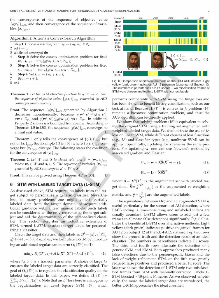
Here we compare STM with both PS1-SVM and PS2-SVM, and summarize the results in Table 5. In all, PS1-SVMshowed the lowest AUC and F1. This outcome occurredbecause of the relatively small number of samples for indi-vidual subjects. Lack of sufficient training data for individ-ual subjects is a common problem for person-specificclassifiers. It is likely that PS1-SVM would have performedthe best if the amount training data from the same subject islarge enough. PS2-SVM achieved better AUC and F1because it sees more training subjects. Overall, STM consis-tently outperformed both PS classifiers.

Selection ability of STM. Recall that PS2 includes samplesof the test subject in both training and test sets. Could STMimprove PS2 performance by selecting proper trainingsamples? To answer this question, we employed PS2 toinvestigate STM’s ability to select relevant training sampleswith respect to the test subject. Table 6 shows the selectionpercentage of STM upon initialization and convergence.Here STM is initialized by KMM. Each row sums to 1 andrepresents a test subject; each entry within one row denotesthe percentage of selected samples from each training sub-ject. For example, (a) shows the initialization phase that,when testing on Subject 2, 26 percent of training samples

Fig. 7. Example images from (a) CK+ [44], (b) GEMEP-FERA [67], and(c) RU-FACS [4] datasets.


IEEE P

roofwere selected from Subject 1. Upon convergence, as (b)

shows, STM selected most training samples that belong tothe target subject (higher diagonal value). Note that theselection percentages along the diagonal do not sum to 100percent due to insufficient training samples for the targetsubject. As a result, STM was able to select relevant trainingsamples, even from different subjects, to alleviate the mis-match between training and test distributions.

8.3.2 Cross-Subject AU Detection

Using a cross-subject scenario, i.e., training and test subjectsare independent in all iterations (a.k.a., leave-one-subject-out), we compared STM against various types of methods.Unsupervised domain adaptation methods are closest toSTM. For comparisons we included Kernel Mean Matching(KMM) [31], Domain Adaptation SVM (DA-SVM) [6], andSubspace Alignment (SA) [25]. Multiple source domainadaptation methods serve as another natural comparison bytreating each training subject as one source domains; wecompared to the state-of-the-art DAM [23]. For baselinemethods, we compared with linear SVMs and semi-super-vised Transductive SVM (T-SVM) [17]. T-SVM, KMM,DAM and SA were implemented per the respective author’swebpage. Because STM requires no target labels, methodsthat use target labels for adaptation (e.g., [19], [40], [54])were not included.

All methods were compared in CK+ and RU-FACS witha few exceptions in CK+. In CK+, SA was ruled out becausetoo few frames were available per subject to compute mean-ingful subspaces. DAM was also omitted in CK+ because it

would be problematic to choose negative samples given thestructure of the data (i.e., pre-segmented positive exam-ples). In training, a Gaussian kernel was used with a band-width set as the median distance between pairwisesamples. For KMM and STM we set B¼1;000 so that none

of si reached the upper bound, and �¼ffiffiffiffiffiffiffiffiffintr�1p ffiffiffiffiffi

ntrp . As reported in

[31], when B was reduced to the point where a small per-centage of the si reached B, empirically performance eitherremained unchanged, or worsened. For T-SVM we used[17] since the original T-SVM [36] solves an integer pro-gramming and thus unscalable to our problem that consistshundreds to thousands of frames. For fairness, we used lin-ear SVMs in all cases. In DA-SVM, we used LibSVM [7] asdiscussed in Section 4, t¼0:5 and b¼0:03. For SA, weobtained the dimension of subspaces dmax using their theo-

retical bound with g¼106 and d¼0:1; SA with both NN andSVM classifiers were reported. Following [23], we tunedDAMusing C¼1, �L¼�D1

¼�D2¼1; bwas set as the median

of computedMMDvalues [5]; the threshold for virtual labelswere cross-validated in f0:01; 0:1; 0:5; 1g. Linear SVMs wereused as base classifiers. Note that, because these alternativemethods are not optimized for our task, their performancesmight be improved by searching over a wider range ofparameters.

Discussion. Tables 7 and 8 show results on AUC and F1scores. A linear SVM served as a generic classifier. Forsemi-supervised learning, T-SVM performed similarly toSVM in RU-FACS, but worse than SVM in CK+. An expla-nation is that in CK+ the negative (neutral) and positive(peak frames) samples are easier to separate than consecu-tive frames in RU-FACS. For transductive transfer learn-ing, KMM performed worse than the generic classifier,

TABLE 5Within-Subject AU Detection with STM and PS Classifiers

TABLE 6Selection Percentage of STM for Different Subjects

TABLE 7Cross-Subject AU Detection on RU-FACS Dataset. “SA (NN|SVM)” Indicates SA with NN and SVM, Respectively


IEEE P

roofbecause KMM estimates sample weights without label

information. SA combined with both Nearest Neighbor(NN) and SVM led to even worse results than the abovemethods. This is because SA obtains an optimal transfor-mation through linear subspace representation, whichcould be improper due to the non-linearity of our data. Inaddition, SA weighted all training samples equally, andthus suffered from biases caused by individual differences(as illustrated in Fig. 2). Although SA+SVM performedbetter in AUC, its low F1 score tells a likely overfitting(low precision or recall). The proposed STM outperformedalternative methods in general. For AUC in RU-FACS,STM achieved the highest averaged score about 6 pointshigher than the 2nd best, and the highest scores in all buttwo AUs. For F1, STM had the highest averaged scoreabout 12 points higher than the nearest alternative, andthe highest F1 score of all but AU4. For CK+, STMachieved 91 percent AUC on average, slightly better thanthe best-published result 90.5 percent [41], although theresults may not be directly comparable due to differentchoices of features and registration. It is noteworthy thatwe tested the last one-third of a video that could containlow intensities, while [41] tested only on peak frames withthe highest intensity. On the other hand, STM may bebenefited from additional frames due to more information.

For other SVM-based methods, unlike STM that uses apenalized SVM, T-SVM considered neither re-weighting fortraining instances nor weight refinement for irrelevant sam-ples, such as noises or outliers. On the other hand, DA-SVMextends T-SVM by progressively labeling test samplesand removing labeled training ones. Not surprisingly,DA-SVM showed better performance than KMM and T-SVM, because it selects relevant samples for training.However, similar to T-SVM, DA-SVM did not update there-weightings using label information. Moreover, it is notalways guaranteed to converge. In our experiments, wefaced the situation where DA-SVM failed to converge dueto a large amount of samples lying within the marginbounds. In contrast, STM is a biconvex formulation, andtherefore is guaranteed to converge to a critical point andoutperformed existing approaches (details in Section 4).

As for multi-source domain adaptation, DAM overallperformed comparably in AUC, but significantly worsethan STM in F1. There are at least three explanations. First,AUs are by nature imbalanced: Simply predicting all sam-ples as negative could yield high AUC for infrequent AUs(such as AUs 4), yet zero precision and recall for F1 score.

Second, similar to person-specific classifiers, training sam-ples for each subject are typically insufficient to estimate thetrue distribution (as discussed in Section 8.3.1). Using suchlimited training samples for each subject, therefore, limitsthe power of base classifiers and the final prediction inDAM. Last but not least, DAM uses MMD to estimate inter-subject distance, which could be inaccurate due to insuffi-cient samples or sampling bias (e.g., some subjects havemore expressions than others).

Although in Table 7 STM achieved slightly worse thanDAM in AUC for some AUs, STM showed a better improve-ment in F1 metric, which more properly describes ourimbalanced detection task. STM’s improvement could belimited due to insufficient training subjects, which hinderSTM from selecting and receiving proper supports from thetraining samples. This can be also explained by the findingsof selection ability in Section 8.3.1. When the number of sub-jects and training samples increase, as will be illustrated inSection 8.5.3, STM is able to gain contributions from theselected data, and thus the improvement becomes moreobvious. Overall STM achieved the most competitive per-formance due to the properties of instance re-weighting,weight refinement, and convergence.

8.3.3 Cross-Dataset AU Detection

Detecting AUs across datasets is challenging because of dif-ferences in acquisition and participant characteristics andbehavior. Fig. 7 shows participant characteristics, context,illumination, camera parameters among the differences thatmay bias features. Generic SVMs fail to address such differ-ences. Sections 8.3.1 and 8.3.2 have shown the effectivenessof STM on within-dataset experiments involving within-sub-ject and across-subject scenarios. This section aims to justifythat STM can attain not only subject adaptation but can benaturally extended for cross-dataset adaptation. Specifically,we performed two experiments, RU-FACS!GEMEP-FERAand GFT!RU-FACS, using the same settings describedabove.

Table 9 shows the results. One can observe that cross-domain approaches outperformed a generic classifier inmost cases. It is not surprising because a generic classifierdoes not model the biases between datasets. That is, inthe cross-dataset scenario, the training and test distribu-tions vary more dramatically than in within-dataset sce-nario, causing a generic classifier to fail to transfer theknowledge from one dataset to another. This alsoexplains why cross-domain approaches showed consis-tent improvements in the cross-dataset setting, comparedto the within-dataset results. Among the cross-domainmethods, STM consistently outperforms the others.Observe STM gained improvement over SVM in Table 7by 12.8 percent in AUC (76.5!86.3) and 33.7 percent inF1 (40.6!54.3), and in Table 9(b) by 37.9 percent in AUC(55.8!77.0) and 46.1 percent in F1 (28.6!41.8). Theadvantages of STM over SVM becomes more obvious inthe cross-dataset experiments.

8.4 Holistic Expression Detection

Taking into account of individual differences, STM showedimprovement for AU detection. In this experiment, we askwhether the same could be found for holistic expression

TABLE 8Cross-Subject AU Detection on CK+ Dataset


IEEE P

roof

detection. We used the major benchmarks CK+ [44] andFERA emotion subchallenge [67] for this experiment, andthe same settings in Section 8.2, except for that the labelswere replaced as holistic expressions. Similar to [67], we uti-lized every frame of a video to train and test our algorithm.Because each video had only a single expression labelinstead of a frame-by-frame labeling, F1 score is meaning-less in this experiment. For CK+, 327 out of the original 593videos were given a nominal expression label based on the7 basic and discrete expressions: Anger, Contempt, Disgust,Fear, Happy, Sadness, and Surprise. For GEMEP-FERA, 289portrayals were retained one out of the five expressionstates: Anger, Fear, Joy, Sadness, and Relief. The training setincluded seven actors with 3 5 instances of each expressionper actor. We evaluated on the training set, which containeda total of 155 videos. STM was also compared to alternativeapproaches discussed in Section 8.3.2.

Table 10(a) shows the results from CK+. Note that DA-SVM is unavailable in this experiment because it failed toconverge to a final classifier due to insufficient test data,recalling that we used the last one-third frames of eachvideo for test. One can observe that a generic SVM per-formed fairly well because positive (peak expressions) andnegative samples (neutral faces) are relatively easy to sepa-rate in CK+. KMM and T-SVM resulted in suboptimalresults due to the lack of a weight-refinement step, and thuswere unable to rectify badly estimated weights for learningthe final classifier (see discussions in Section 7). This effectbecomes obvious when there is insufficient test data, suchas this experiment. On the other hand, STM considers thelabels for weight refinement and performed similarly aswell as a generic SVM.

Table 10(b) presents our results on GEMEP-FERA,which served as a larger and more challenging benchmarkfor evaluating the holistic expression detection perfor-mance. In this experiment, each test video consisted oftens of frames, and thus enabled DA-SVM to converge inmost cases. The generic SVM performed poorly due tolarge variations in this dataset, such as head movementsand exaggerated expressions. Without the ability to selectmeaningful training samples, the generic classifier suf-fered from the individual differences. Other cross-domainmethods alleviated the person-specific biases and pro-duced better results. Overall STM achieved the best aver-aged performance. This also serves as evidence that when

training data grow larger and more complex, the improve-ment of STM becomes clearer.

8.5 Analysis

8.5.1 Initialization Order

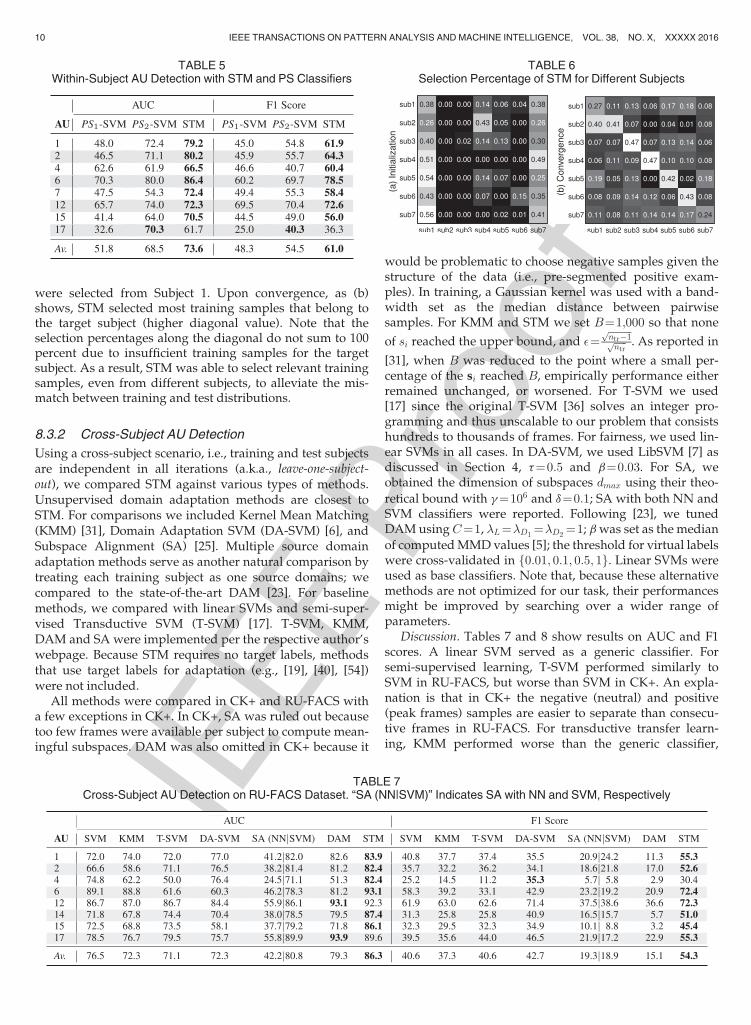
A potential concern of STM is that the initializationorder could affect the convergence property and perfor-mance. To evaluate this, we examined the initializationorder with w0 (STMw) and with s0 (STMs). Standardtwo-stage approach, i.e., solving the selection coefficientsfirst and then the penalized SVM (e.g., [31]), can be inter-preted as STMw, as discussed in Section 4. To validateconvergence property of STM, we randomized 10 initiali-zation sets for STMw and STMs respectively. Upon theconvergence of STM, we computed the objective differ-ences in consecutive iterations (gðztþ1Þ�gðztÞ), and theabsolute sum of variable difference (kztþ1�ztk1). For thecases where STM took fewer iterations to converge, weset the difference of later iterations to 0.

Fig. 8a shows the curve of mean and standard devia-tion of differences across the iterations of STMw andSTMs. Note that the differences were scaled for visuali-zation convenience. The random initial value wasreflected in the first iteration and made a major differ-ence with the value of the second iteration. One can

TABLE 9Cross-Dataset AU Detection: (a) RU-FACS!GEMEP-FERA, and (b) GFT!RU-FACS

(“A!B” Represents for Training on Dataset A and Test on B)

TABLE 10Expression Detection with AUC on (a) CK+

and (b) GEMEP-FERA


IEEE P

roofobserve that in STMw and STMs, both the objective value

and difference between consecutive variables decreasedat each step and toward convergence, as theoreticallydetailed in Section 5. Note that, although the resultingsolution was slightly different due to different initializa-tion, the performance remains the same as both convergeto a critical point. We observed so by comparing the con-fusion matrices during the experiments.

8.5.2 Parameter Choice

Recall that training STM involves two parameters: C forthe tradeoff between maximal margin and training loss,and � for the tradeoff between the SVM empirical riskand the domain mismatch. This section examines the sensi-tivity of performance with respect to different parameterchoices. Specifically, we ran the experiments of detectingAU12 on the CK+ dataset with the parameters ranges

C2f2�10; . . . ; 210g and �2f2�10; . . . ; 210g. Following theexperiment settings in Section 8.2, we computed an aver-aged F1 score for evaluating the performance. We usedGaussian kernel with a fixed bandwidth as the median dis-tance between sample points.

Fig. 8c illustrates the contour plot of F1 scoreversus different parameter pairs in terms of ðlog 2ðCÞ;log 2ð�ÞÞ. As can be observed, the performance scattersevenly in most region of the plot, showing that STM isrobust to the parameter choices when their values arereasonable. The performance decayed when both ðC; �Þbecome extremely small (< 2�6), as shown in the bottomleft of the plot. This is not surprising because smaller val-ues of C and � imply less emphasis on training loss andpersonalization. Note that with large enough �, STMdoes not need large C to achieve comparable F1, provid-ing an explanation that personalization helps avoidimposing large C and hence avoids overfitting. As a gen-eral guideline for choosing parameters, we suggest asmall value of C with a reasonably large � (thus encour-aging a decision boundary with reasonably small distri-bution mismatch).

We note that cross validation (CV) for domain adaptationmethods is difficult and remains an open research issue. Asalso mentioned in [64], this issue becomes vital in a conven-tional scenario where the number of training samples ismuch smaller than the number of test samples. However, inour case, we always have much more training samples thantest samples, and thus, the CV process is less biased undercovariate shift. In addition, as can be seen in Fig. 2 of [64],with proper s (kernel bandwidth) and standard CV, KMM

consistently reaches lower error than the KL-divergence-based CV [64]. This serves as a justification for KMM’sability to estimate importance weights.

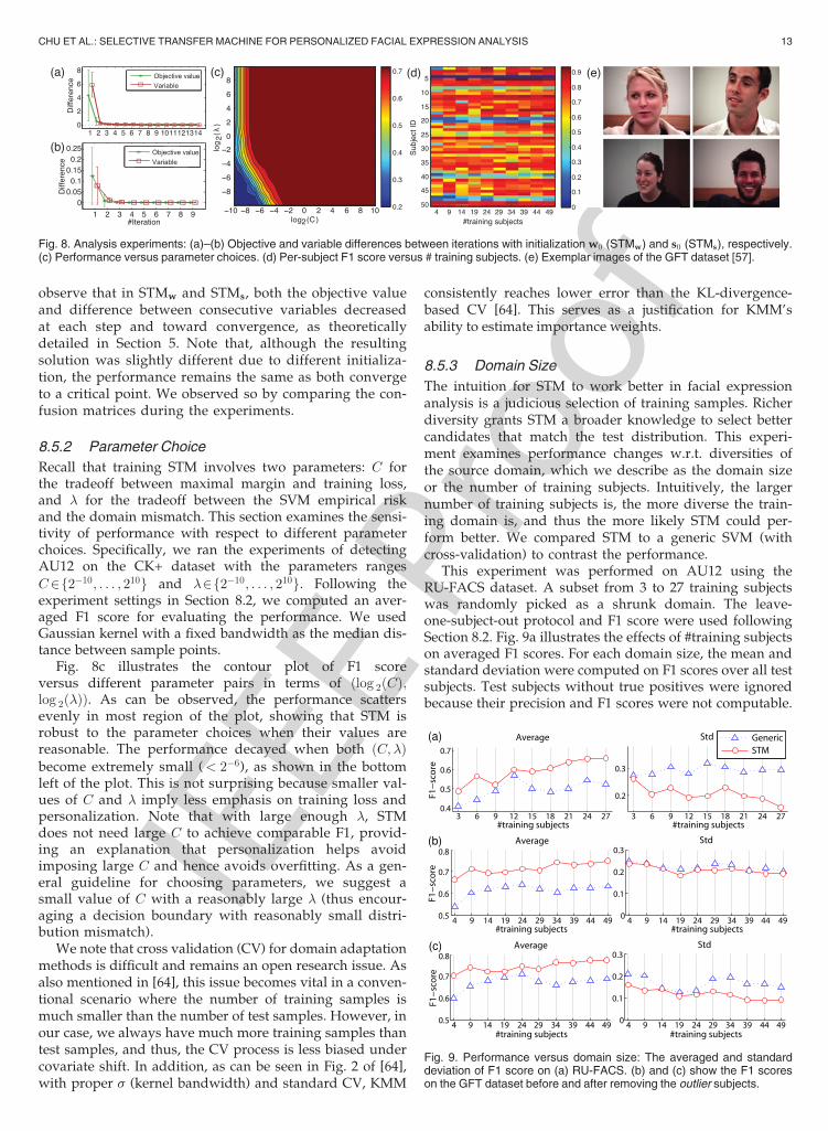
8.5.3 Domain Size

The intuition for STM to work better in facial expressionanalysis is a judicious selection of training samples. Richerdiversity grants STM a broader knowledge to select bettercandidates that match the test distribution. This experi-ment examines performance changes w.r.t. diversities ofthe source domain, which we describe as the domain sizeor the number of training subjects. Intuitively, the largernumber of training subjects is, the more diverse the train-ing domain is, and thus the more likely STM could per-form better. We compared STM to a generic SVM (withcross-validation) to contrast the performance.

This experiment was performed on AU12 using theRU-FACS dataset. A subset from 3 to 27 training subjectswas randomly picked as a shrunk domain. The leave-one-subject-out protocol and F1 score were used followingSection 8.2. Fig. 9a illustrates the effects of #training subjectson averaged F1 scores. For each domain size, the mean andstandard deviation were computed on F1 scores over all testsubjects. Test subjects without true positives were ignoredbecause their precision and F1 scores were not computable.

Fig. 8. Analysis experiments: (a)–(b) Objective and variable differences between iterations with initialization w0 (STMw) and s0 (STMs), respectively.(c) Performance versus parameter choices. (d) Per-subject F1 score versus # training subjects. (e) Exemplar images of the GFT dataset [57].

Fig. 9. Performance versus domain size: The averaged and standarddeviation of F1 score on (a) RU-FACS. (b) and (c) show the F1 scoreson the GFT dataset before and after removing the outlier subjects.


IEEE P

roof

One can observe that, as #training subjects grew, STMachieved higher F1 scores, and also performed more consis-tently with lower standard deviation. This observationimitates Section 8.3.2, where a source domain with poordiversity was shown to limit STM’s performance. On theother hand, the generic classifier improved when #trainingsubjects rose to 12. However, with more training subjectsbeing introduced, its performance was slightly lowered dueto the biases caused by individual differences. Note that,because the training subjects were downsampled in a ran-domized manner, it is possible that STM achieved betterperformance on a domain with less training subjects.

As another justification, we examined the effects ofdomain size on the GFT dataset [57], which contains a largernumber of subjects and more intensive facial expressionsthan RU-FACS. The GFT dataset records videos of real-lifesocial interactions among three-person groups in less con-strained contexts. Videos were recorded using separatewall-mounted cameras facing each subject; Fig. 8e showsexemplar frames. The videos include moderate-to-largehead rotations and frequent occlusions; facial movementsare spontaneous and unscripted. We selected 50 videoswith around 3 minutes each (5,400 frames).

Following the same procedure, we randomly picked asubset of subjects varying from 4 to 49 as the shrunkdomains. Fig. 9b shows the F1 scores with respect to thenumber of training subjects. One can observe the aver-aged F1 score increased with #training subjects, althoughthe standard deviation fluctuated. To study the fluctua-tion, we broke down the averaged F1 into individual sub-jects corresponding to different training sizes, as shownin Fig. 8d. Each row represents a test video; each columnrepresents one number of training subjects (ranging from4 to 49). Note that for subject four (the 4th row), there isno F1 score because AU12 was absent. One can observethat for six outlier subjects (e.g., rows 19, 20, 39, 40, 47,48), their F1 scores remained low even as the number ofsubjects was increased. This result suggests that thesesubjects share no or few instances in the feature space.Visual inspection of their data was consistent with thishypothesis. The outliers were ones with darker skin color,asymmetric smiles or relatively large head pose varia-tions. Thus, for these subjects STM could offer no benefit.This finding suggests the need to include great heteroge-neity in training subjects. When these subjects were omit-ted, as shown in Fig. 9c, the F1 scores are markedlyhigher. The influence of the domain size becomes clearand replicates Fig. 9a. It is interesting to note that, forgeneric classifiers, the performance increased until 24training subjects and then drops abruptly. This obse-rvation serves as another evidence that individual differ-ences (introduced by increasing number of trainingsubjects) could bias generic classifiers.

Between these two experiments, generally the averagedF1 score in GFT is higher than that in RU-FACS. At leasttwo factors may have accounted for this difference. One isthat participants in GFT may have been less inhibited andmore expressive. In RU-FACS, subjects were motivated toconvince an examiner of their veridicality. They knew thatthey would be penalized if they were not believed. In thethree-person social interaction of GFT, there were no such

negative contingencies. Subjects may have felt more relaxedand become more expressive. More intense AUs are moreeasily detected. The other factor is that inter-observer reli-ability of the ground truth FACS labels was likely muchhigher for GFT than for RU-FACS. Kappa coefficients forGFT were exceptionally good. While reliability for RU-FACS is not available, we know from past confirmation-coding that inter-observer agreement was not as high. Lesserror in the GFT ground truth would contribute to moreaccurate classifier performance.

8.6 Discussion

In above experiments, we have evaluated STM against alter-native methods in many scenarios: Within-subject (Sec-tion 8.3.1), cross-subject (Section 8.3.2), cross-dataset(Section 8.3.3), and holistic expression detection (Section 8.4).We also systematically analyzed STM on its initializationorder, and the sensitivity to parameters and domain size(Section 8.5). STM consistently outperformed a generic SVMand most alternative methods. The advantage of STM isclearest in GFT, where the variety of subjects are moreextensive, and slightly so, in RU-FACS. The results indicatea more obvious improvement in F1 than in AUC, in largecomplex datasets than in posed datasets, in cross-datasetscenario than in within-dataset scenario, and with moretraining subjects than with fewer ones.

STM has some limitations. For example, it suffersfrom the lack of training subjects or crucial mismatchbetween training and test distributions, which are knownas common drawbacks in unsupervised domain adapta-tion methods. For a theoretical analysis in terms of per-formance versus the number of samples, Corollary 1.9 inKMM [29] reaches a transductive bound for an estimatedrisk of a re-weighted task, given the assumptions of lin-ear loss and data being iid. However, it remains unclearhow to theoretically analyze STM’s performance in termsof the number of test samples, because STM involvesnonlinear loss functions and the data are from real-worldvideos (non-iid).

9 CONCLUSION AND FUTURE WORK

Based on the observation of individuals differences, wehave presented Selective Transfer Machine for personalizedfacial expression analysis. We showed that STM translatesto a biconvex problem, and proposed an alternating algo-rithm with a primal solution. In addition, we introducedL-STM, an extension of STM that exhibited significantimprovement when labeled test data are available. Ourresults on both AU and holistic expression detection sug-gested that STM is capable of improving test performanceby selecting training samples that form a close distributionto test samples. Experiments using within-subject, cross-subject, and cross-dataset scenarios revealed two insights:(1) Some training data are more instrumental than others,and (2) the effectiveness of STM scales as the number oftraining subjects increases.

It is worth noticing that STM can be extended to other clas-sifiers with convex decision functions and losses, such aslogistic regression. This is a direct outcome of Property 1 inSection 5.1. However, for non-convex cases, such as random


IEEE P

roof

forest, local minimum could cause worse performance. Weleave extensions to non-convex classifiers as a focus of futurework. Moreover, improving STM’s training speed couldbe another direction due to the QP for solving s. Finally, whilethis study focuses evaluations on facial expressions, STMcould be applied to other fields where object-specific issuesare involved, e.g., object or activity recognition.

ACKNOWLEDGMENTS

The authors would like thank many anonymous reviewersfor constructive feedback. Research reported in this paperwas supported in part by the National Institutes of Health(NIH) under Award Number R01MH096951, the NationalScience Foundation (NSF) under the grant RI-1116583, andArmy Research Laboratory Collaborative Technology Alli-ance Program under cooperative agreement W911NF-10-2-0016. The content is solely the responsibility of the authorsand does not necessarily represent the official views of theNIH or the NSF.

REFERENCES

[1] R. Aumann and S. Hart, “Bi-convexity and bi-martingales,” IsraelJ. Math., vol. 54, no. 2, pp. 159–180, 1986.

[2] Y. Aytar and A. Zisserman, “Tabula RASA: Model transfer forobject category detection,” in Proc. IEEE Int. Conf. Comput. Vision,2011, pp. 2252–2259.

[3] M. Baktashmotlagh, M. T. Harandi, B. C. Lovell, andM. Salzmann,“Unsupervised domain adaptation by domain invariant projec-tion,” in Proc. IEEE Int. Conf. Comput. Vision, 2013, pp. 769–776.

[4] M. Bartlett, G. Littlewort, M. Frank, C. Lainscsek, I. Fasel, and J.Movellan, “Automatic recognition of facial actions in spontaneousexpressions,” J. Multimedia, vol. 1, no. 6, pp. 22–35, 2006.

[5] K. M. Borgwardt, A. Gretton, M. J. Rasch, H. P. Kriegel, B.Sch€olkopf, and A. J. Smola, “Integrating structured biological databy kernel maximum mean discrepancy,” Bioinformatics, vol. 22,no. 14, pp. 49–57, 2006.

[6] L. Bruzzone and M. Marconcini, “Domain adaptation problems: ADASVM classification technique and a circular validation strat-egy,” IEEE Trans. Pattern Anal. Mach. Intell., vol. 32, no. 5, pp. 770–787, May 2010.

[7] C.-C. Chang and C.-J. Lin, “LIBSVM: A library for support vectormachines,” ACM Trans. Intell. Syst. Technol., vol. 2, pp. 27:1–27:27,2011.

[8] C.-Y. Chang and V.-C. Huang, “Personalized facial expressionrecognition in indoor environments,” in Proc. Int. Joint Conf. Neu-ral Netw., 2010, pp. 1–8.

[9] K.-Y. Chang, T.-L. Liu, and S.-H. Lai, “Learning partially-observed hidden conditional random fields for facial expressionrecognition,” in Proc. IEEE Conf. Comput. Vis. Pattern Recog., 2009,pp. 533–540.

[10] Y. Chang, C. Hu, R. Feris, and M. Turk, “Manifold based analysisof facial expression,” Image Vision Comput., vol. 24, no. 6, pp. 605–614, 2006.

[11] O. Chapelle, “Training a support vector machine in the primal,”Neural Comput., vol. 19, no. 5, pp. 1155–1178, 2007.

[12] R. Chattopadhyay, Q. Sun, W. Fan, I. Davidson, S. Panchanathan,and J. Ye, “Multi-Source domain adaptation and its application toearly detection of fatigue,” ACM Trans. Knowl. Discovery Data,vol. 6, no. 4, p. 18, 2012.

[13] J. Chen, M. Kim, Y. Wang, and Q. Ji, “Switching Gaussian processdynamic models for simultaneous composite motion tracking andrecognition,” in Proc. IEEE Conf. Comput. Vis. Pattern Recog., 2009,pp. 2655–2662.

[14] J. Chen, X. Liu, P. Tu, and A. Aragones, “Learning person-specificmodels for facial expression and action unit recognition,” PatternRecog. Lett., vol. 34, no. 15, pp. 1964–1970, 2013.

[15] S. W. Chew, P. Lucey, S. Lucey, J. Saragih, J. F. Cohn, and S. Srid-haran, “Person-independent facial expression detection usingconstrained local models,” in Proc. IEEE Int. Conf. Autom. Face Ges-ture Recog., 2011, pp. 915–920.

[16] S. W. Chew, P. Lucey, S. Lucey, J. Saragih, J. F. Cohn, I. Matthews,and S. Sridharan, “In the pursuit of effective affective computing:The relationship between features and registration,” IEEE Trans.Syst., Man, Cybern., Part B: Cybern., vol. 42, no. 4, pp. 1006–1016,Aug. 2012.

[17] R. Collobert, F. Sinz, J. Weston, and L. Bottou, “Large scale trans-ductive SVMs,” J. Mach. Learning Res., vol. 7, pp. 1687–1712, 2006.

[18] T. F. Cootes, G. J. Edwards, and C. J. Taylor, “Active appearancemodels,” IEEE Trans. Pattern Anal. Mach. Intell., vol. 23, no. 6,pp. 681–685, Jun. 2001.

[19] H. Daum�e III, “Frustratingly easy domain adaptation,” in Proc.Conf. Assoc. Comput. Linguistics, 2007, pp. 256–263.

[20] F. De la Torre and J. F. Cohn, “Facial expression analysis,” VisualAnalysis of Humans: Looking at People, p. 377, 2011.

[21] X. Ding, W.-S. Chu, F. De la Torre, and J. F. Cohn, “Facial actionunit event detection by cascade of tasks,” in Proc. IEEE Int. Conf.Comput. Vis., 2013, pp. 2400–2407.

[22] L. Duan, I. W. Tsang, and D. Xu, “Domain transfer multiple kernellearning,” IEEE Trans. Pattern Anal. Mach. Intell., vol. 34, no. 3,pp. 465–479, Mar. 2012.

[23] L. Duan, D. Xu, and I. W. Tsang, “Domain adaptation from multi-ple sources: A domain-dependent regularization approach,” IEEETrans. Neural Netw. Learning Syst., vol. 23, no. 3, pp. 504–518, Mar.2012.

[24] M. Dudık, R. E. Schapire, and S. J. Phillips, “Correcting sampleselection bias in maximum entropy density estimation,” in Proc.Adv. Neural Inf. Process. Syst., 2005, pp. 323–330.

[25] B. Fernando, A. Habrard, M. Sebban, and T. Tuytelaars,“Unsupervised visual domain adaptation using subspacealignment,” inProc. IEEE Int. Conf. Comput. Vis., 2013, pp. 2960–2967.

[26] C. Floudas and V. Visweswaran, “A global optimization algo-rithm (gop) for certain classes of nonconvex nlpsxi. theory,” Com-put. Chem. Eng., vol. 14, no. 12, pp. 1397–1417, 1990.

[27] T. Gehrig and H. K. Ekenel, “A common framework for real-timeemotion recognition and facial action unit detection,” in Proc.IEEE Conf. Comput. Vis. Pattern Recog. Workshop, 2011, pp. 1–6.

[28] J. M. Girard, J. F. Cohn, L. A. Jeni, M. A. Sayette, and F. De laTorre, “Spontaneous facial expression in unscripted social interac-tions can be measured automatically,” Behavior Research Methods,vol. 47, no. 4, pp. 1136-1147, 2014.

[29] D. A. Goldberg, M. B. Goldberg, M. D. Goldberg, and B. M. Gold-berg, “Obtaining person-specific images in a public venue,” U.S.Patent 7,561,723, 2009.

[30] J. Gorski, F. Pfeuffer, and K. Klamroth, “Biconvex sets and optimi-zation with biconvex functions: A survey and extensions,” Math.Methods Operations Res., vol. 66, no. 3, pp. 373–407, 2007.

[31] A. Gretton, A. Smola, J. Huang, M. Schmittfull, K. Borgwardt, andB. Sch€olkopf, “Covariate shift by kernel mean matching,” DatasetShift Mach. Learning, vol. 3, no. 4, pp. 131–160, 2009.

[32] H. Gunes and M. Piccardi, “Affect recognition from face andbody: Early fusion vs. late fusion,” in Proc. Int. Conf. Systems, ManCybern., 2005, vol. 4, pp. 3437–3443.

[33] Y. Guo, G. Zhao, and M. Pietik€ainen, “Dynamic facial expressionrecognition using longitudinal facial expression atlases,” in Proc.10th Eur. Conf. Comput. Vis., 2012, pp. 631–644.

[34] L. A. Jeni, J. F. Cohn, and T. Kanade, “Dense 3d face alignmentfrom 2d videos in real-time,” in Proc. IEEE Int. Conf. Autom. FaceGesture Recog., 2015.

[35] B. Jiang, M. F. Valstar, and M. Pantic, “Action unit detection usingsparse appearance descriptors in space-time video volumes,” inProc. Autom. Face Gesture Recog., 2011, pp. 314–321.

[36] T. Joachims, “Transductive inference for text classification usingsupport vector machines,” in Proc. Int. Conf. Mach. Learn., 1999,pp. 200–209.

[37] T. Kanade, J. F. Cohn, and Y. Tian, “Comprehensive database forfacial expression analysis,” in Proc. Autom. FaceGesture Recog.,2000, pp. 46–53.

[38] A. Kapoor and R. W. Picard, “Multimodal affect recognition inlearning environments,” in Proc. ACM Int. Conf. Multimedia, 2005,pp. 677-682.

[39] A. Khosla, T. Zhou, T. Malisiewicz, A. Efros, and A. Torralba,“Undoing the damage of dataset bias,” in Proc. 10th Eur. Conf.Comput. Vis., 2012, pp. 158-171.

[40] B. Kulis, K. Saenko, and T. Darrell, “What you saw is not whatyou get: Domain adaptation using asymmetric kernel trans-forms,” in Proc. IEEE Conf. Comput. Vis. Pattern Recog., 2011,pp. 1785–1792.


IEEE P

roof

[41] G. Littlewort, J. Whitehill, T. Wu, I. Fasel, M. Frank, J. Movellan,and M. Bartlett, “The computer expression recognition toolbox(CERT),” in Proc. IEEE Int. Conf. Autom. Face Gesture Recog., 2011,pp. 298–305.

[42] M. Liu, S. Li, S. Shan, and X. Chen, “AU-aware deep networks forfacial expression recognition,” in Proc. IEEE Conf. Autom. Face Ges-ture Recog., 2013, pp. 1–6.

[43] B. D. Lucas and T. Kanade, “An iterative image registration tech-nique with an application to stereo vision,” in Proc. Int. Joint Conf.Artif. Intell., 1981, pp. 674–679.

[44] P. Lucey, J. F. Cohn, T. Kanade, J. Saragih, Z. Ambadar, andI. Matthews, “The extended Cohn-Kanade dataset (CK+): Acomplete dataset for action unit and emotion-specifiedexpression,” in Proc. IEEE Conf. Comput. Vis. Pattern Recog.Workshops, 2010, pp. 94–101.

[45] S. Lucey, A. B. Ashraf, and J. Cohn, “Investigating spontaneousfacial action recognition through AAM representations of theface,” Face Recog., pp. 275–286, 2007.

[46] A. Martinez and S. Du, “A model of the perception of facialexpressions of emotion by humans: Research overview andperspectives,” J. Mach. Learning Res., vol. 13, pp. 1589–1608,2012.

[47] I. Matthews and S. Baker, “Active appearance models revisited,”Int. J. Comput. Vis., vol. 60, no. 2, pp. 135–164, 2004.

[48] C. Orrite, A. Ga~n�an, and G. Rogez, “Hog-based decision tree forfacial expression classification,” in Proc. 4th Iberian Conf. PatternRecog. Image Anal., 2009, pp. 176-183.

[49] M. Pantic and M. S. Bartlett, “Machine analysis of facialexpressions,” Face Recog., pp. 377–416, 2007.

[50] J. Quionero-Candela, M. Sugiyama, A. Schwaighofer, and N. Law-rence, Dataset Shift in Machine Learning. Cambridge, MA, USA:MIT Press, 2009.

[51] B. Romera-Paredes, M. S. Aung, M. Pontil, N. Bianchi-Ber-thouze, A. de C Williams, and P. Watson, “Transfer learningto account for idiosyncrasy in face and body expressions,” inProc. 10th IEEE Int. Conf. Workshops Automat. Face GestureRecog., 2013, pp. 1–6.

[52] O. Rudovic, V. Pavlovic, and M. Pantic, “Kernel conditionalordinal random fields for temporal segmentation of facialaction units,” in Proc. Eur. Conf. Comput. Vis. Workshop, 2012,pp. 260–269.

[53] O. Rudovic, V. Pavlovic, and M. Pantic, “Context-sensitivedynamic ordinal regression for intensity estimation of facial actionunits,” IEEE Trans. Pattern Anal. Mach. Intell., vol. 37, no. 5,pp. 944–958, May 2015.

[54] K. Saenko, B. Kulis, M. Fritz, and T. Darrell, “Adapting visual cat-egory models to new domains,” in Proc. Eur. Conf. Comput. Vis.,2010, pp. 213-226.

[55] E. Sangineto, G. Zen, E. Ricci, and N. Sebe, “We are not all equal:Personalizing models for facial expression analysis with transduc-tive parameter transfer,” in Proc. 22nd ACM Int. Conf. Multimedia,2014, pp. 357–366 .

[56] E. Sariyanidi, H. Gunes, and A. Cavallaro, “Automatic analysis offacial affect: A survey of registration, representation, and recog-nition,” IEEE Trans. Pattern Anal. Mach. Intell., vol. 37, no. 6,pp. 1113–1133, Jun. 2015.

[57] M. A. Sayette, K. G. Creswell, J. D. Dimoff, C. E. Fairbairn,J. F. Cohn, B. W. Heckman, T. R. Kirchner, J. M. Levine,and R. L. Moreland, “Alcohol and group formation a multi-modal investigation of the effects of alcohol on emotion andsocial bonding,” Psychological Sci., vol. 23, no. 8, pp. 869–878,2012.

[58] T. Senechal, V. Rapp, H. Salam, R. Seguier, K. Bailly, and L. Pre-vost, “Facial action recognition combining heterogeneous featuresvia multikernel learning,” IEEE Trans. Syst., Man, Cybern., Part B:Cybern., vol. 42, no. 4, pp. 993–1005, Aug. 2012.

[59] L. Shang and K. Chan, “Nonparametric discriminant HMM andapplication to facial expression recognition,” in Proc. IEEE Conf.Comput. Vis. Pattern Recog., 2009, pp. 2090–2096.

[60] K. Sikka, T. Wu, J. Susskind, and M. Bartlett, “Exploring bag ofwords architectures in the facial expression domain,” in Proc. 12thInt. Conf. Comput. Vision, 2012, pp. 250-259.

[61] T. Simon, M. H. Nguyen, F. De La Torre, and J. F. Cohn, “Actionunit detection with segment-based SVMs,” in Proc. IEEE Conf.Comput. Vis. Pattern Recog., 2010, pp. 2737–2744.

[62] J. Sivic and A. Zisserman, “Video Google: A text retrievalapproach to object matching in videos,” in Proc. IEEE Int. Conf.Comput. Vis., 2003, vol. 2, pp. 1470–1477.

[63] M. Sugiyama, M. Krauledat, and K. M€uller, “Covariate shift adap-tation by importance weighted cross validation,” J. Mach. LearningRes., vol. 8, pp. 985–1005, 2007.

[64] M. Sugiyama, S. Nakajima, H. Kashima, P. V. Buenau, and M.Kawanabe, “Direct importance estimation with model selectionand its application to covariate shift adaptation,” in Proc. Adv.Neural Inf. Process. Syst., 2007, pp. 1433–1440.

[65] Y. Tong, W. Liao, and Q. Ji, “Facial action unit recognition byexploiting their dynamic and semantic relationships,” IEEETrans. Pattern Anal. Mach. Intell., vol. 29, no. 10, pp. 1683–1699,Oct. 2007.

[66] A. Torralba and A. Efros, “Unbiased look at dataset bias,” in Proc.IEEE Conf. Comput. Vis. Pattern Recog., 2011, pp. 1521–1528.

[67] M. F. Valstar, M. Mehu, B. Jiang, M. Pantic, and K. Scherer, “Meta-analysis of the first facial expression recognition challenge,” IEEETrans. Syst., Man, Cybern. Part B, vol. 42, no. 4, pp. 966–979, Aug.2012.

[68] M. F. Valstar and M. Pantic, “Fully automatic recognition of thetemporal phases of facial actions,” IEEE Trans. Syst., Man, Cybern.,Part B: Cybern., vol. 42, no. 1, pp. 28–43, Feb. 2012.

[69] T. Van Gestel, J. A. Suykens, B. Baesens, S. Viaene, J. Vanthienen,G. Dedene, B. De Moor, and J. Vandewalle, “Benchmarking leastsquares support vector machine classifiers,” Mach. Learning,vol. 54, no. 1, pp. 5–32, 2004.

[70] Z. Wang, S. Wang, and Q. Ji, “Capturing complex spatio-tem-poral relations among facial muscles for facial expressionrecognition,” in Proc. IEEE Conf. Comput. Vis. Pattern Recog.,2013, pp. 3422–3429.

[71] R. E. Wendell and A. P. Hurter, “Minimization of a non-separableobjective function subject to disjoint constraints,” Operations Res.,vol. 24, no. 4, pp. 643–657, 1976.

[72] J. Whitehill, M. S. Bartlett, and J. R. Movellan, “Automatic facialexpression recognition,” Soc. Emotions Nature Artifact, vol. 88,2013.

[73] T. Wu, M. S. Bartlett, and J. Movellan, “Facial expression recogni-tion using Gabor motion energy filters,” in Proc. IEEE Conf. Com-put. Vis. Pattern Recog. Workshop, 2010, pp. 42–47.

[74] X. Xiong and F. De la Torre, “Supervised descent method and itsapplications to face alignment.” in Proc. IEEE Conf. Comput. Vis.Pattern Recog., 2013, pp. 532–539.

[75] M. Yamada, L. Sigal, and M. Raptis, “No bias left behind: Covari-ate shift adaptation for discriminative 3d pose estimation,” inProc. 12th Eur. Conf. Comput. Vis., 2012, pp. 674–687.

[76] J. Yang, R. Yan, and A. Hauptmann, “Cross-domain video conceptdetection using adaptive SVMs,” in Proc. Int. Conf. Multimedia,2007, pp. 188–197.

[77] P. Yang, Q. Liu, and D. N. Metaxas, “Exploring facial expressionswith compositional features,” in Proc. IEEE Conf. Comput. Vis. Pat-tern Recog., 2010, pp. 2638–2644.

[78] S. Yang, O. Rudovic, V. Pavlovic, and M. Pantic, “Personalizedmodeling of facial action unit intensity,” in Proc. Adv. Visual Com-put., 2014, pp. 269–281.

[79] G. Zen, E. Sangineto, E. Ricci, and N. Sebe, “Unsuperviseddomain adaptation for personalized facial emotion recognition,”in Proc. Int. Conf. Multimodal Interaction, 2014, pp. 128–135.

[80] J. Zeng, W.-S. Chu, F. De la Torre, J. F. Cohn, and Z. Xiong,“Confidence preserving machine for facial action unit detection,”in Proc. IEEE Int. Conf. Comput. Vis., 2015, pp. 3622–3630.

[81] H. Zhang, A. C. Berg, M. Maire, and J. Malik, “SVM-KNN: Dis-criminative nearest neighbor classification for visual category rec-ognition,” in Proc. IEEE Conf. Comput. Vis. Pattern Recog., 2006,pp. 2126–2136.

[82] G. Zhao and M. Pietikainen, “Dynamic texture recognition usinglocal binary patterns with an application to facial expressions,”IEEE Trans. Pattern Anal. Mach. Intell., vol. 29, no. 6, pp. 915–928,Jun. 2007.

[83] K. Zhao, W.-S. Chu, F. De la Torre, J. F. Cohn, and H. Zhang,“Joint patch and multi-label learning for facial action unitdetection,” in Proc. IEEE Conf. Comput. Vis. Pattern Recog.,2015.

[84] L. Zhong, Q. Liu, P. Yang, B. Liu, J. Huang, and D. Metaxas,“Learning active facial patches for expression analysis,” in Proc.IEEE Conf. Comput. Vis. Pattern Recog., 2012, pp. 1499–1510.


IEEE P

roof

[85] F. Zhou, F. De la Torre, and J. F. Cohn, “Unsupervised discoveryof facial events,” in Proc. IEEE Conf. Comput. Vis. Pattern Recog.,2010, pp. 2574–2581.

[86] Y. Zhu, F. De la Torre, J. F. Cohn, and Y. J. Zhang, “Dynamic cas-cades with bidirectional bootstrapping for action unit detection inspontaneous facial behavior,” IEEE Trans. Affective Comput., vol. 2,no. 2, pp. 79–91, Apr.–Jun. 2011.

Wen-Sheng Chu received the BS andMS degrees in computer science from NationalCheng Kung University, Tainan, Taiwan. He iscurrently working toward the PhD degree at theRobotics Institute, Carnegie Mellon University,Pittsburgh, PA, USA. His research interests lie inthe development and use of machine learningtechniques for computer vision problems. He is astudent member of the IEEE and a member ofthe Phi Tau Phi Scholastic Honor Society.

Fernando De la Torre received the BSc degreein telecommunications, as well as the MSc andPhD degrees in electronic engineering from theLa Salle School of Engineering at Ramon LlullUniversity, Barcelona, Spain in 1994, 1996, and2002, respectively. He is an associate researchprofessor in the Robotics Institute at CarnegieMellon University. His research interests are inthe fields of computer vision and machine learn-ing. Currently, he is directing the ComponentAnalysis Laboratory (http://ca.cs.cmu.edu) and

the Human Sensing Laboratory (http://humansensing.cs.cmu.edu) atCarnegie Mellon University. He has more than 150 publications inreferred journals and conferences and is an associate editor at IEEETPAMI. He has organized and co-organized several workshops and hasgiven tutorials at international conferences on component analysis.

Jeffrey F. Cohn is a professor of psychology andpsychiatry at the University of Pittsburgh andadjunct professor of computer science at theRobotics Institute at Carnegie Mellon University.He leads interdisciplinary and inter-institutionalefforts to develop advanced methods of auto-matic analysis and synthesis of facial expressionand prosody; and applies those tools to researchin human emotion, social development, non-ver-bal communication, psychopathology, and bio-medicine. He has served as a Co-Chair of the

2008 IEEE International Conference on Automatic Face and GestureRecognition (FG2008), the 2009 International Conference on AffectiveComputing and Intelligent Interaction (ACII2009), the Steering Commit-tee for IEEE International Conference on Automatic Face and GestureRecognition, and the 2014 International Conference on Multimodal Inter-faces (ACM 2014). He has co-edited special issues of the Journal ofImage and Vision Computing and is a Co-Editor of IEEE Transactions inAffective Computing (TAC).

" For more information on this or any other computing topic,please visit our Digital Library at www.computer.org/publications/dlib.


Documents

IEEE TRANSACTIONS ON PATTERN ANALYSIS AND …jeffcohn/biblio/TPAMI2547397 FINAL.pdf · IEEE Proof Selective Transfer Machine for Personalized Facial Expression Analysis Wen-Sheng