IEEE TRANSACTIONS ON PATTERN ANALYSIS AND ...vision.stanford.edu/teaching/cs231b_spring1415/papers/...input image. The deﬁnition of an ”object” vary. It can be a single instance

IEEE TRANSACTIONS ON PATTERN ANALYSIS AND MACHINE INTELLIGENCE, VOL. 6, NO. 1, JANUARY 2010 1

Tracking-Learning-DetectionZdenek Kalal, Krystian Mikolajczyk, and Jiri Matas,

Abstract—This paper investigates long-term tracking of unknown objects in a video stream. The object is defined by its location andextent in a single frame. In every frame that follows, the task is to determine the object’s location and extent or indicate that the object isnot present. We propose a novel tracking framework (TLD) that explicitly decomposes the long-term tracking task into tracking, learningand detection. The tracker follows the object from frame to frame. The detector localizes all appearances that have been observed sofar and corrects the tracker if necessary. The learning estimates detector’s errors and updates it to avoid these errors in the future. Westudy how to identify detector’s errors and learn from them. We develop a novel learning method (P-N learning) which estimates theerrors by a pair of “experts”: (i) P-expert estimates missed detections, and (ii) N-expert estimates false alarms. The learning process ismodeled as a discrete dynamical system and the conditions under which the learning guarantees improvement are found. We describeour real-time implementation of the TLD framework and the P-N learning. We carry out an extensive quantitative evaluation whichshows a significant improvement over state-of-the-art approaches.

Index Terms—Long-term tracking, learning from video, bootstrapping, real-time, semi-supervised learning

F

1 INTRODUCTIONConsider a video stream taken by a hand-held camera depict-ing various objects moving in and out of the camera’s field ofview. Given a bounding box defining the object of interestin a single frame, our goal is to automatically determinethe object’s bounding box or indicate that the object is notvisible in every frame that follows. The video stream is to beprocessed at frame-rate and the process should run indefinitelylong. We refer to this task as long-term tracking.

To enable the long-term tracking, there are a number ofproblems which need to be addressed. The key problem isthe detection of the object when it reappears in the camera’sfield of view. This problem is aggravated by the fact that theobject may change its appearance thus making the appearancefrom the initial frame irrelevant. Next, a successful long-term tracker should handle scale and illumination changes,background clutter, partial occlusions and operate in real-time.

The long-term tracking can be approached either fromtracking or from detection perspectives. Tracking algorithmsestimate the object motion. Trackers require only initialization,are fast and produce smooth trajectories. On the other hand,they accumulate error during run-time (drift) and typicallyfail if the object disappears from the camera view. Researchin tracking aims at developing increasingly robust trackersthat track “longer”. The post-failure behavior is not directlyaddressed. Detection-based algorithms estimate the object lo-cation in every frame independently. Detectors do not driftand do not fail if the object disappears from the camera view.However, they require an offline training stage and thereforecannot be applied to unknown objects.

• Z. Kalal and K. Mikolajczyk are with the Centre for Vision, Speech andSignal Processing, University of Surrey, Guildford, UK.WWW: http://info.ee.surrey.ac.uk/Personal/Z.Kalal/

• J. Matas is with the Center for Machine Perception, Department ofCybernetics, Faculty of Electrical Engineering, Czech Technical Universityin Prague, Czech Republic.

The starting point of our research is the acceptance of thefact that neither tracking nor detection can solve the long-term tracking task independently. However, if they operatesimultaneously, there is potential to benefit one from another.A tracker can provide weakly labeled training data for adetector and thus improve it during run-time. A detector canre-initialize a tracker and thus minimize the tracking failures.

The first contribution of this paper is the design of a novelframework (TLD) that decomposes the long-term tracking taskinto three sub-tasks: tracking, learning and detection. Eachsub-task is addressed by a single component and the compo-nents operate simultaneously. The tracker follows the objectfrom frame to frame. The detector localizes all appearancesthat have been observed so far and corrects the tracker ifnecessary. The learning estimates detector’s errors and updatesit to avoid these errors in the future.

While a wide range of trackers and detectors exist, we arenot aware of any learning method that would be suitable for theTLD framework. Such a learning method should: (i) deal witharbitrarily complex video streams where the tracking failuresare frequent, (ii) never degrade the detector if the video doesnot contain relevant information and (iii) operate in real-time.

To tackle all these challenges, we rely on the variousinformation sources contained in the video. Consider, forinstance, a single patch denoting the object location in a singleframe. This patch defines not only the appearance of the object,but also determines the surrounding patches, which define theappearance of the background. When tracking the patch, onecan discover different appearances of the same object as wellas more appearances of the background. This is in contrast tostandard machine learning approaches, where a single exampleis considered independent from other examples [1]. This opensinteresting questions how to effectively exploit the informationin the video during learning.

The second contribution of the paper is the new learningparadigm called P-N learning. The detector is evaluated inevery frame of the video. Its responses are analyzed by two


Fig. 1. Given a single bounding box defining the object location and extent in the initial frame (LEFT), our systemtracks, learns and detects the object in real-time. The red dot indicates that the object is not visible.

types of ”experts”: (i) P-expert – recognizes missed detections,and (ii) N-expert – recognizes false alarms. The estimatederrors augment a training set of the detector, and the detectoris retrained to avoid these errors in the future. As any otherprocess, also the P-N experts are making errors them self.However, if the probability of expert’s error is within certainlimits (which will be analytically quantified), the errors aremutually compensated which leads to stable learning.

The third contribution is the implementation. We show howto build a real-time long-term tracking system based on theTLD framework and the P-N learning. The system tracks,learns and detects an object in a video stream in real-time.

The fourth contribution is the extensive evaluation of thestate-of-the-art methods on benchmark data sets, where ourmethod achieved saturated performance. Therefore, we havecollected and annotated new, more challenging data sets, wherea significant improvement over state-of-the-art was achieved.

The rest of the paper is organized as follows. Section 2reviews the work related to the long-term tracking. Section 3introduces the TLD framework and section 4 proposes the P-Nlearning. Section 5 comments on the implementation of TLD.Section 6 then performs a number of comparative experiments.The paper finishes with contributions and suggestions forfuture research.

2 RELATED WORK

This section reviews the related approaches for each of thecomponent of our system. Section 2.1 reviews the objecttracking with the focus on robust trackers that perform onlinelearning. Section 2.2 discusses the object detection. Finally,section 2.3 reviews relevant machine learning approaches fortraining of object detectors.

2.1 Object tracking

Object tracking is the task of estimation of the object motion.Trackers typically assume that the object is visible through-out the sequence. Various representations of the object areused in practice, for example: points [2], [3], [4], articulatedmodels [5], [6], [7], contours [8], [9], [10], [11], or opticalflow [12], [13], [14]. Here we focus on the methods thatrepresent the objects by geometric shapes and their motion isestimated between consecutive frames, i.e. the so-called frame-to-frame tracking. Template tracking is the most straightfor-ward approach in that case. The object is described by a targettemplate (an image patch, a color histogram) and the motion is

defined as a transformation that minimizes mismatch betweenthe target template and the candidate patch. Template trackingcan be either realized as static [15] (when the target templatedoes not change), or adaptive [2], [3] (when the target templateis extracted from the previous frame). Methods that combinestatic and adaptive template tracking have been proposed [16],[17], [18], as well as methods that recognize ”reliable” partsof the template [19], [20]. Templates have limited modelingcapabilities as they represent only a single appearance of theobject. To model more appearance variations, the generativemodels have been proposed. The generative models are eitherbuild offline [21], or during run-time [22], [23]. The generativetrackers model only the appearance of the object and as suchoften fail in cluttered background. In order to alleviate thisproblem, recent trackers also model the environment where theobject moves. Two approaches to environment modeling areoften used. First, the environment is searched for supportingobject the motion of which is correlated with the object of in-terest [24], [25]. These supporting object then help in trackingwhen the object of interest disappears from the camera view orundergoes a difficult transformation. Second, the environmentis considered as a negative class against which the trackershould discriminate. A common approach of discriminativetrackers is to build a binary classifier that represents the deci-sion boundary between the object and its background. Staticdiscriminative trackers [26] train an object classifier beforetracking which limits their applications to known objects.Adaptive discriminative trackers [27], [28], [29], [30] builda classifier during tracking. The essential phase of adaptivediscriminative trackers is the update: the close neighborhoodof the current location is used to sample positive trainingexamples, distant surrounding of the current location is usedto sample negative examples, and these are used to updatethe classifier in every frame. It has been demonstrated thatthis updating strategy handles significant appearance changes,short-term occlusions, and cluttered background. However,these methods also suffer from drift and fail if the object leavesthe scene for longer than expected. To address these problemsthe update of the tracking classifier has been constrained by anauxiliary classifier trained in the first frame [31] or by traininga pair of independent classifiers [32], [33].

2.2 Object detectionObject detection is the task of localization of objects in aninput image. The definition of an ”object” vary. It can be asingle instance or a whole class of objects. Object detection


methods are typically based on the local image features [34]or a sliding window [35]. The feature-based approaches usu-ally follow the pipeline of: (i) feature detection, (ii) featurerecognition, and (iii) model fitting. Planarity [34], [36] or afull 3D model [37] is typically exploited. These algorithmsreached a level of maturity and operate in real-time even onlow power devices [38] and in addition enable detection of alarge number of objects [39], [40]. The main strength as wellas the limitation is the detection of image features and therequirement to know the geometry of the object in advance.The sliding window-based approaches [35], scan the inputimage by a window of various sizes and for each windowdecide whether the underlying patch contains the object ofinterest or not. For a QVGA frame, there are roughly 50,000patches that are evaluated in every frame. To achieve a real-time performance, sliding window-based detectors adopted theso-called cascaded architecture [35]. Exploiting the fact thatbackground is far more frequent than the object, a classifier isseparated into a number of stages, each of which enables earlyrejection of background patches thus reducing the numberof stages that have to be evaluated on average. Training ofsuch detectors typically requires a large number of trainingexamples and intensive computation in the training stage toaccurately represent the decision boundary between the objectand background. An alternative approach is to model the objectas a collection of templates. In that case the learning involvesjust adding one more template [41].

2.3 Machine learning

Object detectors are traditionally trained assuming that alltraining examples are labeled. Such an assumption is toostrong in our case since we wish to train a detector froma single labeled example and a video stream. This problemcan be formulated as a semi-supervised learning [42], [43]that exploits both labeled and unlabeled data. These methodstypically assume independent and identically distributed datawith certain properties, such as that the unlabeled examplesform “natural” clusters in the feature space. A number ofalgorithms relying on similar assumptions have been proposedin the past including EM, Self-learning and Co-training.

Expectation-Maximization (EM) is a generic method forfinding estimates of model parameters given unlabeled data.EM is an iterative process, which in case of binary classifica-tion alternates over estimation of soft-labels of unlabeled dataand training a classifier. EM was successfully applied to docu-ment classification [44] and learning of object categories [45].In the semi-supervised learning terminology, EM algorithmrelies on the ”low density separation” assumption [42], whichmeans that the classes are well separated. EM is sometimesinterpreted as a “soft” version of self-learning [43].

Self-learning starts by training an initial classifier from alabeled training set, the classifier is then evaluated on theunlabeled data. The examples with the most confident classifierresponses are added to the training set and the classifier isretrained. This is an iterative process. The self-learning hasbeen applied to human eye detection in [46]. However, it wasobserved that the detector improved more if the unlabeled

Fig. 2. The block diagram of the TLD framework.

data was selected by an independent measure rather than theclassifier confidence. It was suggested that the low densityseparation assumption is not satisfied for object detection andother approaches may work better.

Co-training [1] is a learning method build on the idea thatindependent classifiers can mutually train one another. Tocreate such independent classifiers, co-training assumes thattwo independent feature-spaces are available. The learningis initialized by training of two separate classifiers usingthe labeled examples. Both classifiers are then evaluated onunlabeled data. The confidently labeled samples from thefirst classifier are used to augment the training set of thesecond classifier and vice versa in an iterative process. Co-training works best for problems with independent modalities,e.g. text classification [1] (text and hyper-links) or biometricrecognition systems [47] (appearance and voice). In visualobject detection, co-training has been applied to car detectionin surveillance [48] and moving object recognition [49]. Weargue that co-training is suboptimal for object detection, sincethe examples (image patches) are sampled from a singlemodality. Features extracted from a single modality may bedependent and therefore violate the assumptions of co-training.

2.4 Most related approachesMany approaches combine tracking, learning and detectionin some sense. In [50], an offline trained detector is used tovalidate the trajectory output by a tracker and if the trajectoryis not validated, an exhaustive image search is performed tofind the target. Other approaches integrate the detector withina particle filtering [51] framework. Such techniques have beenapplied to tracking of faces in low frame-rate video [52],multiple hockey players [53], or pedestrians [54], [55]. Incontrast to our method, these methods rely on an offline traineddetector that does not change its properties during run-time.Adaptive discriminative trackers [29], [30], [31], [32], [33]also have the capability to track, learn and detect. Thesemethods realize tracking by an online learned detector thatdiscriminates the target from its background. In other words,a single process represents both tracking and detection. Thisis in contrast to our approach where tracking and detectionare independent processes that exchange information usinglearning. By keeping the tracking and detection separated ourapproach does not have to compromise neither on tracking nordetection capabilities of its components.


Training

P-Nexperts

Classifier

unlabeled data

TrainingSet

labeled data

labels

classifierparameters

[+] examples

[-] examples

Fig. 3. The block diagram of the P-N learning.

3 TRACKING-LEARNING-DETECTIONTLD is a framework designed for long-term tracking of anunknown object in a video stream. Its block diagram isshown in figure 2. The components of the framework arecharacterized as follows: Tracker estimates the object’s motionbetween consecutive frames under the assumption that theframe-to-frame motion is limited and the object is visible.The tracker is likely to fail and never recover if the objectmoves out of the camera view. Detector treats every frameas independent and performs full scanning of the image tolocalize all appearances that have been observed and learnedin the past. As any other detector, the detector makes twotypes of errors: false positives and false negative. Learningobserves performance of both, tracker and detector, estimatesdetector’s errors and generates training examples to avoid theseerrors in the future. The learning component assumes that boththe tracker and the detector can fail. By the virtue of thelearning, the detector generalizes to more object appearancesand discriminates against background.

4 P-N LEARNINGThis section investigates the learning component of the TLDframework. The goal of the component is to improve theperformance of an object detector by online processing ofa video stream. In every frame of the stream, we wish toevaluate the current detector, identify its errors and updateit to avoid these errors in the future. The key idea of P-Nlearning is that the detector errors can be identified by twotypes of “experts”. P-expert identifies only false negatives, N-expert identifies only false positives. Both of the experts makeerrors themselves, however, their independence enables mutualcompensation of their errors.

Section 4.1 formulates the P-N learning as a semi-supervised learning method. Section 4.2 models the P-N learn-ing as a discrete dynamical system and finds conditions underwhich the learning guarantees improvement of the detector.Section 4.3 performs several experiments with syntheticallygenerated experts. Finally, section 4.4 applies the P-N learningto training object detectors from video and proposes expertsthat could be used in practice.

4.1 FormalizationLet x be an example from a feature-space X and y be a labelfrom a space of labels Y = {−1, 1}. A set of examples X

is called an unlabeled set, Y is called a set of labels andL = {(x, y)} is called a labeled set. The input to the P-Nlearning is a labeled set Ll and an unlabeled set Xu, wherel � u. The task of P-N learning is to learn a classifier f :X → Y from labeled set Ll and bootstrap its performanceby the unlabeled set Xu. Classifier f is a function from afamily F parameterized by Θ. The family F is subject toimplementation and is considered fixed in training, the trainingtherefore corresponds to estimation of the parameters Θ.

The P-N learning consists of four blocks: (i) a classifier tobe learned, (ii) training set – a collection of labeled trainingexamples, (iii) supervised training – a method that trains aclassifier from training set, and (iv) P-N experts – functionsthat generate positive and negative training examples duringlearning. See figure 3 for illustration.

The training process is initialized by inserting the labeledset L to the training set. The training set is then passed tosupervised learning which trains a classifier, i.e. estimates theinitial parameters Θ0. The learning process then proceeds byiterative bootstrapping. In iteration k, the classifier trained inprevious iteration classifies the entire unlabeled set, yku =f(xu|Θk−1) for all xu ∈ Xu. The classification is analyzedby the P-N experts which estimate examples that have beenclassified incorrectly. These examples are added with changedlabels to the training set. The iteration finishes by retrainingthe classifier, i.e. estimation of Θk. The process iterates untilconvergence or other stopping criterion.

The crucial element of P-N learning is the estimation ofthe classifier errors. The key idea is to separate the estimationof false positives from the estimation of false negatives. Forthis reason, the unlabeled set is split into two parts basedon the current classification and each part is analyzed by anindependent expert. P-expert analyzes examples classified asnegative, estimates false negatives and adds them to trainingset with positive label. In iteration k, P-expert outputs n+(k)positive examples. N-expert analyzes examples classified aspositive, estimates false positives and adds them with neg-ative label to the training set. In iteration k, the N-expertoutputs n−(k) negative examples. The P-expert increases theclassifier’s generality. The N-expert increases the classifier’sdiscriminability.

Relation to supervised bootstrap. To put the P-N learninginto broader context, let us consider that the labels of setXu are known. Under this assumption it is straightforward torecognize misclassified examples and add them to the trainingset with correct labels. Such a strategy is commonly called(supervised) bootstraping [56]. A classifier trained using suchsupervised bootstrap focuses on the decision boundary andoften outperforms a classifier trained on randomly sampledtraining set [56]. The same idea of focusing on the decisionboundary underpins the P-N learning with the difference thatthe labels of the set Xu are unknown. P-N learning cantherefore be viewed as a generalization of standard bootstrap tounlabeled case where labels are not given but rather estimatedusing the P-N experts. As any other process, also the P-N experts make errors by estimating the labels incorrectly.Such errors propagate through the training, which will betheoretically analyzed in the following section.


4.2 Stability

This section analyses the impact of the P-N learning on theclassifier performance. We assume an abstract classifier (e.g.nearest neighbour) the performance of which is measuredon Xu. The classifier initially classifies the unlabeled set atrandom and then corrects its classification for those examplesthat were returned by the P-N experts. For the purpose ofthe analysis, let us consider that the labels of Xu are known.This will allow us to measure both the classifier errors and theerrors of the P-N experts. The performance of this classifierwill be characterized by a number of false positives α(k) and anumber of false negatives β(k), where k indicates the iterationof training.

In iteration k, the P-expert outputs n+c (k) positive exampleswhich are correct (positive based on the ground truth), andn+f (k) positive examples which are false (negative basedon the ground truth), which forces the classifier to changen+(k) = n+c (k) + n+f (k) negatively classified examplesto positive. Similarly, the N-experts outputs n−c (k) correctnegative examples and n−f (k) false negative examples, whichforces the classifier to change n−(k) = n−c (k) + n−f (k)examples classified as positive to negative. The false positiveand false negative errors of the classifier in the next iterationthus become:

α(k + 1) = α(k)− n−c (k) + n+f (k) (1a)

β(k + 1) = β(k)− n+c (k) + n−f (k). (1b)

Equation 1a shows that false positives α(k) decrease ifn−c (k) > n+f (k), i.e. number of examples that were correctlyrelabeled to negative is higher than the number of examplesthat were incorrectly relabeled to positive. Similarly, the falsenegatives β(k) decrease if n+c (k) > n−f (k).

Quality measures. In order to analyze the convergence ofthe P-N learning, a model needs to be defined that relates thequality of the P-N experts to the absolute number of positiveand negative examples output in each iteration. The quality ofthe P-N experts is characterized by four quality measures:

• P-precision – reliability of the positive labels, i.e. thenumber of correct positive examples divided by thenumber of all positive examples output by the P-expert,P+ = n+c /(n

+c + n+f ).

• P-recall – percentage of identified false negative errors,i.e. the number of correct positive examples divided bythe number of false negatives output by the classifier,R+ = n+c / β.

• N-precision – reliability of negative labels, i.e. the numberof correct negative examples divided by the number ofall positive examples output by the N-expert, P− =n−c /(n

−c + n−f ).

• N-recall – percentage of recognized false positive errors,i.e. the number of correct negative examples divided bythe number of all false positives output by the classifier,R− = n−c /α.

Given these quality measures, the number of correct andfalse examples output by P-N experts at iteration k have the

l1=0, l2< 1

a

b b b

a a

l1=0, l2=1 l1

=0, l2> 1

Fig. 4. Evolution of errors during P-N learning for differ-ent eigenvalues of matrix M. The errors are decreasing(LEFT), are static (MIDDLE) or grow (RIGHT).

following form:

n+c (k) = R+ β(k), n+f (k) =(1− P+)

P+R+ β(k) (2a)

n−c (k) = R− α(k), n−f (k) =(1− P−)

P−R− α(k). (2b)

By combining the equation 1a, 1b, 2a and 2b we obtain thefollowing equations:

α(k + 1) = (1−R−)α(k) +(1− P+)

P+R+ β(k) (3a)

β(k + 1) =(1− P−)

P−R− α(k) + (1−R+)β(k). (3b)

After defining the state vector ~x(k) =[α(k) β(k)

]Tand a

2× 2 matrix M as

M =

[1−R− (1−P+)

P+ R+

(1−P−)P− R− (1−R+)

](4)

it is possible to rewrite the equations as

~x(k + 1) = M~x(k).

This is a recursive equations that correspond to a discretedynamical system. The system shows how the error of theclassifier (encoded by the system state) propagates from oneiteration of P-N learning to another. Our goal is to show, underwhich conditions the error in the system drops.

Based on the well founded theory of dynamical systems[57], [58], the state vector ~x converges to zero if both eigen-values λ1, λ2 of the transition matrix M are smaller than one.Note that the matrix M is a function of the expert’s qualitymeasures. Therefore, if the quality measures are known, itallows the determine the stability of the learning. Experts forwhich corresponding matrix M has both eigenvalues smallerthan one will be called error-canceling. Figure 4 illustratesthe evolution of error of the classifier when λ1 = 0 and (i)λ2 < 1, (ii) λ2 = 1, (iii) λ2 > 1.

In the above analysis the quality measures were assumed tobe constant and the classes separable. In practice, it is not notpossible to identify all the errors of the classifier. Therefore,the training does not converge to error-less classifier, butmay stabilize at a certain level. In case the quality measurevary, the performance increases in those iterations where theeigenvalues of M are smaller than one.


0 1000

0

1

Number of Frames Processed

F-M

easu

re

0.0

0.5

0.6

Fig. 5. Performance of a detector as a function of thenumber of processed frames. The detectors were trainedby synthetic P-N experts with certain level of error. Theclassifier is improved up to error 50% (BLACK), highererror degrades it (RED).

4.3 Experiments with simulated experts

In this experiment, a classifier is trained on a real sequenceusing simulated P-N experts. Our goal is to analyze thelearning performance as a function of the expert’s qualitymeasures.

The analysis is carried on sequence CAR (see figure 12).In the first frame of the sequence, we train a random forrestclassifier using affine warps of the initial patch and the back-ground from the first frame. Next, we perform a single run overthe sequence. In every frame, the classifier is evaluated, thesimulated experts identify errors and the classifier is updated.After every update, the classifier is evaluated on the entiresequence to measure its performance using f-measure. Theperformance is then drawn as a function of the number ofprocessed frames and the quality of the P-N experts.

The P-N experts are characterized by four quality measures,P+, R+, P−, R−. To reduce this 4D space, the parameters areset to P+ = R+ = P− = R− = 1 − ε, where ε representserror of the expert. The transition matrix then becomes M =ε1, where 1 is a 2x2 matrix with all elements equal to 1. Theeigenvalues of this matrix are λ1 = 0, λ2 = 2ε. Therefore theP-N learning should be improving the performance if ε < 0.5.The error is varied in the range ε = 0 : 0.9.

The experts are simulated as follows. In frame k, the classi-fier generates β(k) false negatives. P-expert relabels n+c (k) =(1− ε)β(k) of them to positive which gives R+ = 1− ε. Inorder to simulate the required precision P+ = 1 − ε, the P-expert relabels additional n+f (k) = ε β(k) background samplesto positive. Therefore, the total number of examples relabeledto positive in iteration k is n+ = n+c (k)+n+f (k) = β(k). TheN-experts were generated similarly.

The performance of the detector as a function of number ofprocessed frames is depicted in figure 5. Notice that if ε ≤ 0.5the performance of the detector increases with more trainingdata. In general, ε = 0.5 will give unstable results although inthis sequence it leads to improvements. Increasing the noise-level further leads to sudden degradation of the classifier.These results are in line with the P-N Learning theory.

a) scanning grid b) unacceptable labeling c) acceptable labeling

Fig. 6. Illustration of a scanning grid and correspondingvolume of labels. Red dots correspond to positive labels.

4.4 Design of real experts

This section applies the P-N learning to training an objectdetector from a labeled frame and a video stream. The de-tector consists of a binary classifier and a scanning window,and the training examples correspond to image patches. Thelabeled examples Xl are extracted from the labeled frame. Theunlabeled data Xu are extracted from the video stream.

The P-N learning is initialized by supervised training ofso-called initial detector. In every frame, the P-N learningperforms the following steps: (i) evaluation of the detectoron the current frame, (ii) estimation of the detector errorsusing the P-N experts, (iii) update of the detector by labeledexamples output by the experts. The detector obtained at theend of the learning is called the final detector.

Figure 6 (a) that shows three frames of a video sequenceoverlaid with a scanning grid. Every bounding box in the griddefines an image patch, the label of which is represented asa colored dot in (b,c). Every scanning window-based detectorconsiders the patches as independent. Therefore, there are 2N

possible label combinations in a single frame, where N is thenumber of bounding boxes in the grid. Figure 6 (b) shows onesuch labeling. The labeling indicates, that the object appearsin several locations in a single frame and that there is notemporal continuity in the motion. Such labeling is unlikelyto be correct. On the other hand, if the detector outputs resultsdepicted in (c) the labeling is plausible since the object appearsat one location in each frame and the detected locations buildup a trajectory in time. In other words, the labels of the patchesare dependent. We refer to such a property as structure. Thekey idea of the P-N experts is to exploit the structure in datato identify the detector errors.

P-expert exploits the temporal structure in the video andassumes that the object moves along a trajectory. The P-expertremembers the location of the object in the previous frame andestimates the object location in current frame using a frame-to-frame tracker. If the detector labeled the current location asnegative (i.e. made false negative error), the P-expert generatesa positive example.

N-expert exploits the spatial structure in the video andassumes that the object can appear at a single location only.The N-expert analyzes all responses of the detector in thecurrent frame and the response produced by the tracker andselects the one that is the most confident. Patches that are notoverlapping with the maximally confident patch are labeledas negative. The maximally confident patch re-initializes thelocation of the tracker.

Figure 7 depicts a sequence of three frames, the object


Fig. 7. Illustration of the examples output by the P-Nexperts. The third row shows error compensation.

to be learned is a car within the yellow bounding box. Thecar is tracked from frame to frame by a tracker. The trackerrepresents the P-expert that outputs positive training examples.Notice that due to occlusion of the object, the output of P-expert in time t + 2 outputs incorrect positive example. N-expert identifies maximally confident patch (denoted by a redstar) and labels all other detections as negative. Notice that theN-expert is discriminating against another car, and in additioncorrected the error made by the P-expert in time t+ 2.

5 IMPLEMENTATION OF TLDThis section describes our implementation of the TLD frame-work. The block diagram is shown in figure 8.

5.1 Prerequisites

At any time instance, the object is represented by its state.The state is either a bounding box or a flag indicating thatthe object is not visible. The bounding box has a fixed aspectratio (given by the initial bounding box) and is parameterizedby its location and scale. Other parameters such as in-planerotation are not considered. Spatial similarity of two boundingboxes is measured using overlap, which is defined as a ratiobetween intersection and union.

A single instance of the object’s appearance is representedby an image patch p. The patch is sampled from an imagewithin the object bounding box and then is re-sampled to anormalized resolution (15x15 pixels) regardless of the aspectratio. Similarity between two patches pi, pj is defined as

S(pi, pj) = 0.5(NCC(pi, pj) + 1), (5)

where NCC is a Normalized Correlation Coefficient.A sequence of object states defines a trajectory of an object

in a video volume as well as the corresponding trajectoryin the appearance (feature) space. Note that the trajectory isfragmented as the object may not be visible.

5.2 Object model

Object model M is a data structure that representsthe object and its surrounding observed so far. It isa collection of positive and negative patches, M =

Tracking

Detection

Inte

gra

tor Object

stateLearning

updatedetector

Videoframe

Object model

Objectstate

updatetracker

Fig. 8. Detailed block diagram of the TLD framework.

{p+1 , p+2 , . . . , p

+m, p

−1 , p

−2 , . . . , p

−n }, where p+ and p− repre-

sent the object and background patches, respectively. Positivepatches are ordered according to the time when the patch wasadded to the collection. p+1 represents the first positive patchadded to the collection, p+m is the positive patch added last.

Given an arbitrary patch p and object model M , we defineseveral similarity measures:

1) Similarity with the positive nearest neighbor,S+(p,M) = maxp+

i ∈MS(p, p+i ).

2) Similarity with the negative nearest neighbor,S−(p,M) = maxp−

i ∈MS(p, p−i ).

3) Similarity with the positive nearest neighbor consid-ering 50% earliest positive patches, S+

50%(p,M) =maxp+

i ∈M∧

i<m2S(p, p+i ).

4) Relative similarity, Sr = S+

S++S− . Relative similarityranges from 0 to 1, higher values mean more confidentthat the patch depicts the object.

5) Conservative similarity, Sc =S+50%

S+50%

+S− . Conservativesimilarity ranges from 0 to 1. High value of Sc meanmore confidence that the patch resembles appearanceobserved in the first 50% of the positive patches.

Nearest Neighbor (NN) classifier. The similarity measures(Sr, Sc) are used throughout TLD to indicate how muchan arbitrary patch resembles the appearances in the model.The Relative similarity is used to define a nearest neighborclassifier. A patch p is classified as positive if Sr(p,M) > θNNotherwise the patch is classified as negative. A classificationmargin is defined as Sr(p,M)− θNN. Parameter θNN enablestuning the NN classifier either towards recall or precision.

Model update. To integrate a new labeled patch to theobject model we use the following strategy: the patch isadded to the collection only if the its label estimated by NNclassifier is different from the label given by the P-N experts.This leads to a significant reduction of accepted patches atthe cost of coarser representation of the decision boundary.Therefore we improve this strategy by adding also patcheswhere the classification margin is smaller than λ. With largerλ, the model accepts more patches which leads to betterrepresentation of the decision boundary. In our experiments weuse λ = 0.1 which compromises the accuracy of representationand the speed of growing of the object model. Exact settingof this parameter is not critical.


Ensemble classifier 1-NN classifier

Patch

variance

Rejected patches

Accepted

patches

( ,..., )

1

1

2

32

3

Fig. 9. Block diagram of the object detector.

5.3 Object detector

The detector scans the input image by a scanning-window andfor each patch decides about presence or absence of the object.

Scanning-window grid. We generate all possible scales andshifts of an initial bounding box with the following parameters:scales step = 1.2, horizontal step = 10% of width, verticalstep = 10% of height, minimal bounding box size = 20 pixels.This setting produces around 50k bounding boxes for a QVGAimage (240x320), the exact number depends on the aspect ratioof the initial bounding box.

Cascaded classifier. As the number of bounding boxesto be evaluated is large, the classification of every singlepatch has to be very efficient. A straightforward approachof directly evaluating the NN classifier is problematic as itinvolves evaluation of the Relative similarity (i.e. search fortwo nearest neighbours). As illustrated in figure 9, we structurethe classifier into three stages: (i) patch variance, (ii) ensembleclassifier, and (iii) nearest neighbor. Each stage either rejectsthe patch in question or passes it to the next stage. In ourprevious work [59] we used only the first two stages. Lateron, we observed that the performance improves if the thirdstage is added. Templates allowed us to better estimate thereliability of the detection.

5.3.1 Patch variance

Patch variance is the first stage of our cascade. This stagerejects all patches, for which gray-value variance is smallerthan 50% of variance of the patch that was selected fortracking. The stage exploits the fact that gray-value varianceof a patch p can be expressed as E(p2) − E2(p), and thatthe expected value E(p) can be measured in constant timeusing integral images [35]. This stage typically rejects morethan 50% of non-object patches (e.g. sky, street). The variancethreshold restricts the maximal appearance change of theobject. However, since the parameter is easily interpretable,it can be adjusted by a user for particular application. In allof our experiments we kept it constant.

5.3.2 Ensemble classifier

Ensemble classifier is the second stage of our detector. The in-put to the ensemble is an image patch that was not rejected bythe variance filter. The ensemble consists of n base classifiers.Each base classifier i performs a number of pixel comparisonson the patch resulting in a binary code x, which indexes to anarray of posteriors Pi(y|x), where y ∈ {0, 1}. The posteriorsof individual base classifiers are averaged and the ensembleclassifies the patch as the object if the average posterior islarger than 50%.

1

0

0

0

1

1

0

1

1

1

pixel comparisons binary codeinput image + bounding box

blur measure

blurred image

output

Fig. 10. Conversion of a patch to a binary code.

Pixel comparisons. Every base classifier is based on a setof pixel comparisons. Similarly as in [60], [61], [62], the pixelcomparisons are generated offline at random and stay fixed inrun-time. First, the image is convolved with a Gaussian kernelwith standard deviation of 3 pixels to increase the robustnessto shift and image noise. Next, the predefined set of pixelcomparison is stretched to the patch. Each comparison returns0 or 1 and these measurements are concatenated into x.

Generating pixel comparisons. The vital element of en-semble classifiers is the independence of the base classi-fiers [63]. The independence of the classifiers is in our caseenforced by generating different pixel comparisons for eachbase classifier. First, we discretize the space of pixel locationswithin a normalized patch and generate all possible horizontaland vertical pixel comparisons. Next, we permutate the com-parisons and split them into the base classifiers. As a result,every classifier is guaranteed to be based on a different set offeatures and all the features together uniformly cover the entirepatch. This is in contrast to standard approaches [60], [61],[62], where every pixel comparison is generated independentof other pixel comparisons.

Posterior probabilities. Every base classifier i maintains adistribution of posterior probabilities Pi(y|x). The distributionhas 2d entries, where d is the number of pixel comparisons.We use 13 comparison, which gives 8192 possible codes thatindex to the posterior probability. The probability is estimatedas Pi(y|x) = #p

#p+#n , where #p and #n correspond tonumber of positive and negative patches, respectively, thatwere assigned the same binary code.

Initialization and update. In the initialization stage, allbase posterior probabilities are set to zero, i.e. vote for negativeclass. During run-time the ensemble classifier is updated asfollows. The labeled example is classified by the ensembleand if the classification is incorrect, the corresponding #pand #n are updated which consequently updates Pi(y|x).

5.3.3 Nearest neighbor classifierAfter filtering the patches by the variance filter and the ensem-ble classifier, we are typically left with several of boundingboxes that are not decided yet (≈ 50). Therefore, we can usethe online model and classify the patch using a NN classifier.A patch is classified as the object if Sr(p,M) > θNN, whereθNN = 0.6. This parameter has been set empirically and itsvalue is not critical. We observed that similar performanceis achieved in the range (0.5-0.7). The positively classifiedpatches represent the responses of the object detector. Whenthe number of templates in NN classifier exceeds some thresh-old (given by memory), we use random forgetting of templates.We observed that the number of templates stabilizes around


several hundred which can be easily stored in memory.

5.4 TrackerThe tracking component of TLD is based on Median-Flowtracker [64] extended with failure detection. Median-Flowtracker represents the object by a bounding box and estimatesits motion between consecutive frames. Internally, the trackerestimates displacements of a number of points within theobject’s bounding box, estimates their reliability, and voteswith 50% of the most reliable displacements for the motion ofthe bounding box using median. We use a grid of 10×10 pointsand estimate their motion using pyramidal Lucas-Kanadetracker [65]. Lucas-Kanade uses 2 levels of the pyramid andrepresents the points by 10× 10 patches.

Failure detection. Median-Flow [64] tracker assumes visi-bility of the object and therefore inevitably fails if the objectgets fully occluded or moves out of the camera view. Toidentify these situations we use the following strategy. Let didenote the displacement of a single point of the Median-Flowtracker and dm be the median displacement. A residual of asingle displacement is then defined as |di − dm|. A failure ofthe tracker is declared if median|di − dm|>10 pixels. Thisstrategy is able to reliably identify failures caused by fastmotion or fast occlusion of the object of interest. In thatcase, the individual displacement become scattered around theimage and the residual rapidly increases (the threshold of 10pixels is not critical). If the failure is detected, the tracker doesnot return any bounding box.

5.5 IntegratorIntegrator combines the bounding box of the tracker and thebounding boxes of the detector into a single bounding boxoutput by TLD. TIf neither the tracker not the detector outputa bounding box, the object is declared as not visible. Other-wise the integrator outputs the maximally confident boundingbox, measured using Conservative similarity Sc. The trackerand detector have identical priorities, however they representfundamentally different estimates of the object state. Whilethe detector localizes already known templates, the trackerlocalizes potentially new templates and thus can bring newdata for detector.

5.6 Learning componentThe task of the learning component is to initialize the objectdetector in the first frame and update the detector in run-timeusing the P-expert and the N-expert. An alternative explanationof the experts, called growing and pruning, can be foundin [66].

5.6.1 InitializationIn the first frame, the learning component trains the initialdetector using labeled examples generated as follows. Thepositive training examples are synthesized from the initialbounding box. First we select 10 bounding boxes on thescanning grid that are closest to the initial bounding box. Foreach of the bounding box, we generate 20 warped versions

Fig. 11. Illustration of P-expert: a) object model andthecore in feature space (gray blob), b) unreliable (dotted)and reliable (thick) trajectory , c) the object model and thecore after the update. Red dots are positive examples,black dots are negative, cross denotes end of a trajectory.

by geometric transformations (shift ±1%, scale change ±1%,in-plane rotation ±10◦) and add them with Gaussian noise(σ = 5) on pixels. The result is 200 synthetic positive patches.Negative patches are collected from the surrounding of theinitializing bounding box, no synthetic negative examples aregenerated. If the application requires fast initialization, we sub-sample the generated training examples. The labeled trainingpatches are then used to update the object model as discussedin subsection 5.2 and the ensemble classifier as discussed insubsection 5.3. After the initialization the object detector isready for run-time and to be updated by a pair of P-N experts.

5.6.2 P-expertThe goal of P-expert is to discover new appearances of theobject and thus increase generalization of the object detector.Section 4.4 suggested that the P-expert can exploit the factthat the object moves on a trajectory and add positive examplesextracted from such a trajectory. However, in the TLD system,the object trajectory is generated by a combination of a tracker,detector and the integrator. This combined process traces adiscontinuous trajectory, which is not correct all the time. Thechallenge of the P-expert is to identify reliable parts of thetrajectory and use it to generate positive training examples.

To identify the reliable parts of the trajectory, the P-expertrelies on an object model M . See figure 11 for reference.Consider an object model represented as colored points in afeature space. Positive examples are represented by red dotsconnected by a directed curve suggesting their order, negativeexamples are black. Using the conservative similarity Sc, onecan define a subset in the feature space, where Sc is largerthan a threshold. We refer to this subset as the core of theobject model. Note that the core is not a static structure, butit grows as new examples are coming to the model. However,the growth is slower than the entire model.

P-expert identifies the reliable parts of the trajectory asfollows. The trajectory becomes reliable as soon as it entersthe core and remain reliable until is re-initialized or the trackeridentifies its own failure. Figure 11 (b) illustrates the reliableand non-reliable trajectory in feature space. And figure 11(c) shows how the core changes after accepting new positiveexamples from reliable trajectory.

In every frame, the P-expert outputs a decision about thereliability of the current location (P-expert is an online pro-cess). If the current location is reliable, the P-expert generates


a set of positive examples that update the object model andthe ensemble classifier. We select 10 bounding boxes on thescanning grid that are closest to the current bounding box. Foreach of the bounding box, we generate 10 warped versionsby geometric transformations (shift ±1%, scale change ±1%,in-plane rotation ±5◦) and add them with Gaussian noise(σ = 5). The result is 100 synthetic positive examples forensemble classifier.

5.6.3 N-expertN-expert generates negative training examples. Its goal is todiscover clutter in the background against which the detectorshould discriminate. The key assumption of the N-expert isthat the object can occupy at most one location in the image.Therefore, if the object location is known, the surrounding ofthe location is labeled as negative. The N-expert is appliedat the same time as P-expert, i.e. if the trajectory is reliable.In that case, patches that are far from current bounding box(overlap < 0.2) are all labeled as negative. For the update ofthe object detector and the ensemble classifier, we consideronly those patches that were not rejected neither by thevariance filter nor the ensemble classifier.

6 QUANTITATIVE EVALUATION

This section reports on a set of quantitative experimentscomparing the TLD with relevant algorithms. The first twoexperiments (section 6.1, section 6.2) evaluate our system onbenchmark sequences that are commonly used in the litera-ture. In both of these experiments, a saturated performanceis achieved. Section 6.3 therefore introduces a new, morechallenging dataset. Using this dataset, section 6.4 focuseson evaluation of the learning component of TLD. Finally,section 6.5 evaluates the whole system.

Every experiment in this section adopts the following eval-uation protocol. A tracker is initialized in the first frame of asequence and tracks the object of interest up to the end. Theproduced trajectory is then compared to ground truth using anumber of measures specified in the particular experiment.

6.1 Comparison 1: CoGDTLD was compared with results reported in [33] which re-ports on performance of 5 trackers (Iterative Visual Track-ing (IVT) [22], Online Discriminative Features (ODV) [27],Ensemble Tracking (ET) [28], Multiple Instance Learning(MIL) [30], and Co-trained Generative-Discriminative track-ing (CoGD) [33]) on 6 sequences. The sequences includefull occlusions and disappearance of the object. CoGD [33]dominated on these sequences as it enabled re-detection ofthe object. As in [33], the performance was accessed usingthe Number of successfully tracked frames, i.e. the number offrames where overlap with a ground truth bounding box islarger than 50%. Frames where the object was occluded werenot counted. For instance, for a sequence of 100 frames with20 occluded frames, the maximal possible score is 80.

Table 1 shows the results. TLD achieved the maximalpossible score in the sequences and matched the performanceof CoGD [33]. It was reported in [33] that CoGD runs at

TABLE 1Number of successfully tracked frames – TLD in

comparison to results reported in [33].

Sequence Frames Occ. IVT ODF ET MIL CoGD TLD[22] [27] [28] [30] [33]

David *761 0 17 - 94 135 759 761Jumping 313 0 75 313 44 313 313 313Pedestrian 1 140 0 11 6 22 101 140 140Pedestrian 2 338 93 33 8 118 37 240 240Pedestrian 3 184 30 50 5 53 49 154 154Car 945 143 163 - 10 45 802 802

TABLE 2Recall – TLD1.0 in comparison to results reported

in [67]. Bold font means the best score.

Sequence Frames OB ORF FT MIL Prost TLD[29] [68] [20] [30] [67]

Girl 452 24.0 - 70.0 70.0 89.0 93.1David 502 23.0 - 47.0 70.0 80.0 100.0Sylvester 1344 51.0 - 74.0 74.0 73.0 97.4Face occlusion 1 858 35.0 - 100.0 93.0 100.0 98.9Face occlusion 2 812 75.0 - 48.0 96.0 82.0 96.9Tiger 354 38.0 - 20.0 77.0 79.0 88.7Board 698 - 10.0 67.9 67.9 75.0 87.1Box 1161 - 28.3 61.4 24.5 91.4 91.8Lemming 1336 - 17.2 54.9 83.6 70.5 85.8Liquor 1741 - 53.6 79.9 20.6 83.7 91.7Mean - 42.2 27.3 58.1 64.8 80.4 92.5

2 frames per second, and requires several frames (typically6) for initialization. In contrast, TLD requires just a singleframe and runs at 20 frames per second. This experimentdemonstrates that neither the generative trackers (IVT [22]),nor the discriminative trackers (ODF [27], ET [28], MIL [30])are able to handle full occlusions or disappearance of theobject. CoGD will be evaluated in detail in section 6.5.

6.2 Comparison 2: ProstTLD was compared with the results reported in [67] whichreports on performance of 5 algorithms (Online Boosting(OB) [29], Online Random Forrest (ORF) [68], Fragment-baset Tracker (FT) [20], MIL [30] and Prost [67]) on 10benchmark sequences. The sequences include partial occlu-sions and pose changes. The performance was reported usingtwo measures: (i) Recall - number of true positives divided bythe length of the sequence (true positive is considered if theoverlap with ground truth is > 50%), and (ii) Average local-ization Error - average distance between center of predictedand ground truth bounding box. TLD estimates scale of anobject. However, the algorithms compared in this experimentperform tracking in single scale only. In order to make a faircomparison, the scale estimation was not used.

Table 2 shows the performance measured by Recall. TLDscored best in 9/10 outperforming by more than 12% thesecond best (Prost [67]). Table 2 shows the performancemeasured by Average localization error. TLD scored best in7/10 being 1.6 times more accurate than the second best.

6.3 TLD datasetThe experiments 6.1 and 6.2 show that TLD performs wellon benchmark sequences. We consider these sequences assaturated and therefore introduce new, more challenging data


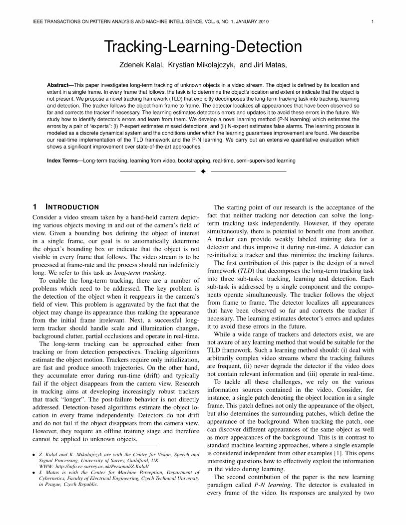
TABLE 3Average localization error – TLD in comparison to results

reported in [67]. Bold means best.

Sequence Frames OB ORF FT MIL Prost TLD[29] [68] [20] [30] [67]

Girl 452 43.3 - 26.5 31.6 19.0 18.1David 502 51.0 - 46.0 15.6 15.3 4.0Sylvester 1344 32.9 - 11.2 9.4 10.6 5.9Face occlusion 1 858 49.0 - 6.5 18.4 7.0 15.4Face occlusion 2 812 19.6 - 45.1 14.3 17.2 12.6Tiger 354 17.9 - 39.6 8.4 7.2 6.4Board 698 - 154.5 154.5 51.2 37.0 10.9Box 1161 - 145.4 145.4 104.5 12.1 17.4Lemming 1336 - 166.3 166.3 14.9 25.4 16.4Liquor 1741 - 67.3 67.3 165.1 21.6 6.5Mean - 32.9 133.4 78.0 46.1 18.4 10.9

TABLE 4TLD dataset

Name Frames Mov. Partial Full Pose Illum. Scale Similarcamera occ. occ. change change change objects

1. David 761 yes yes no yes yes yes no2. Jumping 313 yes no no no no no no3. Pedestrian 1 140 yes no no no no no no4. Pedestrian 2 338 yes yes yes no no no yes5. Pedestrian 3 184 yes yes yes no no no yes6. Car 945 yes yes yes no no no yes7. Motocross 2665 yes yes yes yes yes yes yes8. Volkswagen 8576 yes yes yes yes yes yes yes9. Carchase 9928 yes yes yes yes yes yes yes10. Panda 3000 yes yes yes yes yes yes no

set. We started from the 6 sequences used in experiment 6.1and collected 4 additional sequences: Motocross, Volkswagen,Carchase and Panda. The new sequences are long and containall the challenges typical for long-term tracking. Table 4 liststhe properties of the sequences and figure 12 shows corre-sponding snapshots. The sequences were manually annotated.More than 50% of occlusion or more than 90 degrees of out-of-plane rotation was annotated as ”not visible”.

The performance is evaluated using precision P , recall Rand f-measure F . P is the number of true positives divided bynumber of all responses, R is the number true positives dividedby the number of object occurrences that should have beendetected. F combines these two measures as F = 2PR/(P +R). A detection was considered to be correct if its overlapwith ground truth bounding box was larger than 50%.

6.4 Improvement of the object detector

This experiment quantitatively evaluates the learning com-ponent of the TLD system on the TLD dataset. For everysequence, we compare the Initial Detector (trained in the firstframe) and the Final Detector (obtained after one pass throughthe training). Next, we measure the quality of the P-N experts(P+, R+, P−,R−) in every iteration of the learning and reportthe average score.

Table 5 shows the achieved results. The scores of theInitial Detector are shown in the 3rd column. Precision isabove 79% high except for sequence 9, which contains asignificant background clutter and objects similar to the target(cars). Recall is low for the majority of sequences except forsequence 5 where the recall is 73%. High recall indicates thatthe appearance of the object does not vary significantly andtraining the Initial Detector is sufficient.

The scores of the Final Detector are displayed in the 4thcolumn. Recall of the detector was significantly increased withlittle drop of precision. In sequence 9, even the precision wasincreased from 36% to 90%, which shows that the false pos-itives of the Initial Detector were identified by N-experts andcorrected. Most significant increase of the performance is forsequences 7-10 which are the most challenging of the wholeset. The Initial Detector fails here but for the Final Detectorthe f-measure in the range of 25-83%. This demonstrates theimprovement of the detector using P-N learning.

The last three columns of Table 5 report the performanceof P-N experts. Both experts have precision higher than 60%except for sequence 10 which has P-precision just 31%. Recallof the experts is in the range of 2-78%. The last column showsthe corresponding eigenvalues of matrix M. Notice that alleigenvalues are smaller than one. This demonstrates that theproposed experts work across different scenarios. The largerthese eigenvalues are, the less the P-N learning improves theperformance. For example in sequence 10 one eigenvalue is0.99 which reflects poor performance of the P-N experts. Thetarget of this sequence is an animal which performs out-of-plane motion. Median-Flow tracker is not very reliable inthis scenario, but still P-N learning exploits the informationprovided by the tracker and improves the detector.

6.5 Comparison 3: TLD datasetThis experiment evaluates the proposed system on the TLDdataset and compares it to five trackers: (1) OB [29], (2)SB [31], (3) BS [69], (4) MIL [30], and (5) CoGD [33].Binaries for trackers (1-3) are available in the Internet1.Trackers (4,5) were kindly evaluated directly by their authors.

Since this experiment compares various trackers for whichthe default initialization (defined by ground truth) might notbe optimal, we allowed the initialization to be selected by theauthors. For instance, when tracking a motorbike racer, somealgorithms might perform better when tracking only a partof the racer. When comparing thus obtained trajectories toground truth, we performed normalization (shift, aspect andscale correction) of the trajectory so that the first boundingbox matched the ground truth, all remaining bounding boxeswere normalized with the same parameters. The normalizedtrajectory was then directly compared to ground truth usingoverlap and true positive was considered if the overlap waslarger than 25%. As we allowed different initialization, theearlier used threshold 50% was found to be too restrictive.

Sequences Motocross and Volkswagen were evaluated bythe MIL tracker [30] only up to the frame 500 as the algorithmrequired loading all images into memory in advance. Since thealgorithm failed during this period, the remaining frames wereconsidered as failed.

Table 6 show the achieved performance evaluated byprecision/recall/f-measure. The last row shows a weightedaverage performance (weighted by number of frames in thesequence). Considering the overall performance accessed byF-measure, TLD achieved the best performance of 81% signif-icantly outperforming the second best approach that achieved

1. http://www.vision.ee.ethz.ch/boostingTrackers/


TABLE 5Performance analysis of P-N learning. The Initial Detector is trained on the first frame. The Final Detector is trained

using the proposed P-N learning. The last three columns show internal statistics of the training process.

Sequence Frames Initial Detector Final Detector P-expert N-expert EigenvaluesPrecision / Recall / F-measure Precision / Recall / F-measure P+, R+ P−, R− λ1, λ2

1. David 761 1.00 / 0.01 / 0.02 1.00 / 0.32 / 0.49 1.00 / 0.08 0.99 / 0.17 0.92 / 0.832. Jumping 313 1.00 / 0.01 / 0.02 0.99 / 0.88 / 0.93 0.86 / 0.24 0.98 / 0.30 0.70 / 0.773. Pedestrian 1 140 1.00 / 0.06 / 0.12 1.00 / 0.12 / 0.22 0.81 / 0.04 1.00 / 0.04 0.96 / 0.964. Pedestrian 2 338 1.00 / 0.02 / 0.03 1.00 / 0.34 / 0.51 1.00 / 0.25 1.00 / 0.24 0.76 / 0.755. Pedestrian 3 184 1.00 / 0.73 / 0.84 0.97 / 0.93 / 0.95 0.98 / 0.78 0.98 / 0.68 0.32 / 0.226. Car 945 1.00 / 0.04 / 0.08 0.99 / 0.82 / 0.90 1.00 / 0.52 1.00 / 0.46 0.48 / 0.547. Motocross 2665 1.00 / 0.00 / 0.00 0.92 / 0.32 / 0.47 0.96 / 0.19 0.84 / 0.08 0.92 / 0.818. Volkswagen 8576 1.00 / 0.00 / 0.00 0.92 / 0.75 / 0.83 0.70 / 0.23 0.99 / 0.09 0.91 / 0.779. Car Chase 9928 0.36 / 0.00 / 0.00 0.90 / 0.42 / 0.57 0.64 / 0.19 0.95 / 0.22 0.76 / 0.8310. Panda 3000 0.79 / 0.01 / 0.01 0.51 / 0.16 / 0.25 0.31 / 0.02 0.96 / 0.19 0.81 / 0.99

1. David 2. Jumping 3. Pedestrian 1 4. Pedestrian 2 5. Pedestrian 3

6. Car 8. Volkswagen 9. Car Chase 10. Panda7. Motocross

Fig. 12. Snapshots from the introduced TLD dataset.

22%, other approaches range between 13-15%. The sequenceshave been processed with identical parameters with exceptionfor sequence Panda, where any positive example added to themodel had been augmented with mirrored version.

CONCLUSIONS

In this paper, we studied the problem of tracking of anunknown object in a video stream, where the object changesappearance frequently moves in and out of the camera view.We designed a new framework that decomposes the tasks intothree components: tracking, learning and detection. The learn-ing component was analyzed in detail. We have demonstratedthat an object detector can be trained from a single exampleand an unlabeled video stream using the following strategy:(i) evaluate the detector, (ii) estimate its errors by a pair ofexperts, and (iii) update the classifier. Each expert is focusedon identification of particular type of the classifier error andis allowed to make errors itself. The stability of the learningis achieved by designing experts that mutually compensatetheir errors. The theoretical contribution is the formalizationof this process as a discrete dynamical system, which allowedus to specify conditions, under which the learning processguarantees improvement of the classifier. We demonstratedthat the experts can exploit spatio-temporal relationships inthe video. A real-time implementation of the framework has

been described in detail. And an extensive set of experimentswas performed. Superiority of our approach with respect tothe closest competitors was clearly demonstrated. The codeof the algorithm as well as the TLD dataset has been madeavailable online2.

LIMITATIONS AND FUTURE WORKThere are a number of challenges that have to be addressed inorder to get more reliable and general system based on TLD.For instance, TLD does not perform well in case of full out-of-plane rotation. In that case the, the Median-Flow trackerdrifts away from the target and can be re-initialized onlyif the object reappears with appearance seen/learned before.Current implementation of TLD trains only the detector andthe tracker stay fixed. As a result the tracker makes alwaysthe same errors. An interesting extension would be to trainalso the tracking component. TLD currently tracks a singleobject. Multi-target tracking opens interesting questions howto jointly train the models and share features in order toscale. Current version does not perform well for articulatedobjects such as pedestrians. In case of restricted scenarios,e.g. static camera, an interesting extension of TLD would beto include background subtraction in order to improve thetracking capabilities.

2. http://cmp.felk.cvut.cz/tld


Sequence Frames OB [29] SB [31] BS [69] MIL [30] CoGD [33] TLD1. David 761 0.41 / 0.29 / 0.34 0.35 / 0.35 / 0.35 0.32 / 0.24 / 0.28 0.15 / 0.15 / 0.15 1.00 / 1.00 / 1.00 1.00 / 1.00 / 1.002. Jumping 313 0.47 / 0.05 / 0.09 0.25 / 0.13 / 0.17 0.17 / 0.14 / 0.15 1.00 / 1.00 / 1.00 1.00 / 0.99 / 1.00 1.00 / 1.00 / 1.003. Pedestrian 1 140 0.61 / 0.14 / 0.23 0.48 / 0.33 / 0.39 0.29 / 0.10 / 0.15 0.69 / 0.69 / 0.69 1.00 / 1.00 / 1.00 1.00 / 1.00 / 1.004. Pedestrian 2 338 0.77 / 0.12 / 0.21 0.85 / 0.71 / 0.77 1.00 / 0.02 / 0.04 0.10 / 0.12 / 0.11 0.72 / 0.92 / 0.81 0.89 / 0.92 / 0.915. Pedestrian 3 184 1.00 / 0.33 / 0.49 0.41 / 0.33 / 0.36 0.92 / 0.46 / 0.62 0.69 / 0.81 / 0.75 0.85 / 1.00 / 0.92 0.99 / 1.00 / 0.996. Car 945 0.94 / 0.59 / 0.73 1.00 / 0.67 / 0.80 0.99 / 0.56 / 0.72 0.23 / 0.25 / 0.24 0.95 / 0.96 / 0.96 0.92 / 0.97 / 0.947. Motocross 2665 0.33 / 0.00 / 0.01 0.13 / 0.03 / 0.05 0.14 / 0.00 / 0.00 0.05 / 0.02 / 0.03 0.93 / 0.30 / 0.45 0.89 / 0.77 / 0.838. Volkswagen 8576 0.39 / 0.02 / 0.04 0.04 / 0.04 / 0.04 0.02 / 0.01 / 0.01 0.42 / 0.04 / 0.07 0.79 / 0.06 / 0.11 0.80 / 0.96 / 0.879. Carchase 9928 0.79 / 0.03 / 0.06 0.80 / 0.04 / 0.09 0.52 / 0.12 / 0.19 0.62 / 0.04 / 0.07 0.95 / 0.04 / 0.08 0.86 / 0.70 / 0.7710. Panda 3000 0.95 / 0.35 / 0.51 1.00 / 0.17 / 0.29 0.99 / 0.17 / 0.30 0.36 / 0.40 / 0.38 0.12 / 0.12 / 0.12 0.58 / 0.63 / 0.60mean 26850 0.62 / 0.09 / 0.13 0.50 / 0.10 / 0.14 0.39 / 0.10 / 0.15 0.44 / 0.11 / 0.13 0.80 / 0.18 / 0.22 0.82 / 0.81 / 0.81

TABLE 6Performance evaluation on TLD dataset measured by Precision/Recall/F-measure. Bold numbers indicate the best

score. TLD1.0 scored best in 9/10 sequences.

ACKNOWLEDGMENTSThe research was supported by the UK EPSRC EP/F0034 20/1and BBC R&D grants (KM and ZK) and by EC project FP7-ICT-270138 Darwin and Czech Science Foundation projectGACR P103/10/1585 (JM).

REFERENCES[1] A. Blum and T. Mitchell, “Combining labeled and unlabeled data with

co-training,” Conference on Computational Learning Theory, p. 100,1998.

[2] B. D. Lucas and T. Kanade, “An iterative image registration techniquewith an application to stereo vision,” International Joint Conference onArtificial Intelligence, vol. 81, pp. 674–679, 1981.

[3] J. Shi and C. Tomasi, “Good features to track,” Conference on ComputerVision and Pattern Recognition, 1994.

[4] P. Sand and S. Teller, “Particle video: Long-range motion estimationusing point trajectories,” International Journal of Computer Vision,vol. 80, no. 1, pp. 72–91, 2008.

[5] L. Wang, W. Hu, and T. Tan, “Recent developments in human motionanalysis,” Pattern Recognition, vol. 36, no. 3, pp. 585–601, 2003.

[6] D. Ramanan, D. A. Forsyth, and A. Zisserman, “Tracking people bylearning their appearance,” IEEE Transactions on Pattern Analysis andMachine Intelligence, pp. 65–81, 2007.

[7] P. Buehler, M. Everingham, D. P. Huttenlocher, and A. Zisserman,“Long term arm and hand tracking for continuous sign language TVbroadcasts,” British Machine Vision Conference, 2008.

[8] S. Birchfield, “Elliptical head tracking using intensity gradients and colorhistograms,” Conference on Computer Vision and Pattern Recognition,1998.

[9] M. Isard and A. Blake, “CONDENSATION - Conditional DensityPropagation for Visual Tracking,” International Journal of ComputerVision, vol. 29, no. 1, pp. 5–28, 1998.

[10] C. Bibby and I. Reid, “Robust real-time visual tracking using pixel-wiseposteriors,” European Conference on Computer Vision, 2008.

[11] C. Bibby and I. Reid, “Real-time Tracking of Multiple OccludingObjects using Level Sets,” Computer Vision and Pattern Recognition,2010.

[12] B. K. P. Horn and B. G. Schunck, “Determining optical flow,” Artificialintelligence, vol. 17, no. 1-3, pp. 185–203, 1981.

[13] T. Brox, A. Bruhn, N. Papenberg, and J. Weickert, “High accuracyoptical flow estimation based on a theory for warping,” EuropeanConference on Computer Vision, pp. 25–36, 2004.

[14] J. L. Barron, D. J. Fleet, and S. S. Beauchemin, “Performance of OpticalFlow Techniques,” International Journal of Computer Vision, vol. 12,no. 1, pp. 43–77, 1994.

[15] D. Comaniciu, V. Ramesh, and P. Meer, “Kernel-Based Object Track-ing,” IEEE Transactions on Pattern Analysis and Machine Intelligence,vol. 25, no. 5, pp. 564–577, 2003.

[16] I. Matthews, T. Ishikawa, and S. Baker, “The Template Update Prob-lem,” IEEE Transactions on Pattern Analysis and Machine Intelligence,vol. 26, no. 6, pp. 810–815, 2004.

[17] N. Dowson and R. Bowden, “Simultaneous Modeling and Tracking(SMAT) of Feature Sets,” Conference on Computer Vision and PatternRecognition, 2005.

[18] A. Rahimi, L. P. Morency, and T. Darrell, “Reducing drift in differentialtracking,” Computer Vision and Image Understanding, vol. 109, no. 2,pp. 97–111, 2008.

[19] A. D. Jepson, D. J. Fleet, and T. F. El-Maraghi, “Robust OnlineAppearance Models for Visual Tracking,” IEEE Transactions on PatternAnalysis and Machine Intelligence, pp. 1296–1311, 2003.

[20] A. Adam, E. Rivlin, and I. Shimshoni, “Robust Fragments-based Track-ing using the Integral Histogram,” Conference on Computer Vision andPattern Recognition, pp. 798–805, 2006.

[21] M. J. Black and A. D. Jepson, “Eigentracking: Robust matching andtracking of articulated objects using a view-based representation,” Inter-national Journal of Computer Vision, vol. 26, no. 1, pp. 63–84, 1998.

[22] D. Ross, J. Lim, R. Lin, and M. Yang, “Incremental Learning for RobustVisual Tracking,” International Journal of Computer Vision, vol. 77,pp. 125–141, Aug. 2007.

[23] J. Kwon and K. M. Lee, “Visual Tracking Decomposition,” Conferenceon Computer Vision and Pattern Recognition, 2010.

[24] M. Yang, Y. Wu, and G. Hua, “Context-aware visual tracking.,” IEEEtransactions on pattern analysis and machine intelligence, vol. 31,pp. 1195–209, July 2009.

[25] H. Grabner, J. Matas, L. Van Gool, and P. Cattin, “Tracking the Invisible:Learning Where the Object Might be,” Conference on Computer Visionand Pattern Recognition, 2010.

[26] S. Avidan, “Support Vector Tracking,” IEEE Transactions on PatternAnalysis and Machine Intelligence, pp. 1064–1072, 2004.

[27] R. Collins, Y. Liu, and M. Leordeanu, “Online Selection of Discrimi-native Tracking Features,” IEEE Transactions on Pattern Analysis andMachine Intelligence, vol. 27, no. 10, pp. 1631–1643, 2005.

[28] S. Avidan, “Ensemble Tracking,” IEEE Transactions on Pattern Analysisand Machine Intelligence, vol. 29, no. 2, pp. 261–271, 2007.

[29] H. Grabner and H. Bischof, “On-line boosting and vision,” Conferenceon Computer Vision and Pattern Recognition, 2006.

[30] B. Babenko, M.-H. Yang, and S. Belongie, “Visual Tracking withOnline Multiple Instance Learning,” Conference on Computer Visionand Pattern Recognition, 2009.

[31] H. Grabner, C. Leistner, and H. Bischof, “Semi-Supervised On-lineBoosting for Robust Tracking,” European Conference on ComputerVision, 2008.

[32] F. Tang, S. Brennan, Q. Zhao, H. Tao, and U. C. Santa Cruz, “Co-tracking using semi-supervised support vector machines,” InternationalConference on Computer Vision, pp. 1–8, 2007.

[33] Q. Yu, T. B. Dinh, and G. Medioni, “Online tracking and reacquisi-tion using co-trained generative and discriminative trackers,” EuropeanConference on Computer Vision, 2008.

[34] D. G. Lowe, “Distinctive image features from scale-invariant keypoints,”International Journal of Computer Vision, vol. 60, no. 2, pp. 91–110,2004.

[35] P. Viola and M. Jones, “Rapid object detection using a boosted cas-cade of simple features,” Conference on Computer Vision and PatternRecognition, 2001.

[36] V. Lepetit, P. Lagger, and P. Fua, “Randomized trees for real-timekeypoint recognition,” Conference on Computer Vision and PatternRecognition, 2005.

[37] L. Vacchetti, V. Lepetit, and P. Fua, “Stable real-time 3d tracking usingonline and offline information,” IEEE Transactions on Pattern Analysisand Machine Intelligence, vol. 26, no. 10, p. 1385, 2004.


[38] S. Taylor and T. Drummond, “Multiple target localisation at over 100fps,” British Machine Vision Conference, 2009.

[39] J. Pilet and H. Saito, “Virtually augmenting hundreds of real pictures: Anapproach based on learning, retrieval, and tracking,” 2010 IEEE VirtualReality Conference (VR), pp. 71–78, Mar. 2010.

[40] S. Obdrzalek and J. Matas, “Sub-linear indexing for large scale objectrecognition,” British Machine Vision Conference, vol. 1, pp. 1–10, 2005.

[41] S. Hinterstoisser, O. Kutter, N. Navab, P. Fua, and V. Lepetit, “Real-time learning of accurate patch rectification,” Conference on ComputerVision and Pattern Recognition, 2009.

[42] O. Chapelle, B. Scholkopf, and A. Zien, Semi-Supervised Learning.Cambridge, MA: MIT Press, 2006.

[43] X. Zhu and A. B. Goldberg, Introduction to semi-supervised learning.Morgan & Claypool Publishers, 2009.

[44] K. Nigam, A. K. McCallum, S. Thrun, and T. Mitchell, “Text clas-sification from labeled and unlabeled documents using EM,” MachineLearning, vol. 39, no. 2, pp. 103–134, 2000.

[45] R. Fergus, P. Perona, and A. Zisserman, “Object class recognition byunsupervised scale-invariant learning,” Conference on Computer Visionand Pattern Recognition, vol. 2, 2003.

[46] C. Rosenberg, M. Hebert, and H. Schneiderman, “Semi-supervisedself-training of object detection models,” Workshop on Application ofComputer Vision, 2005.

[47] N. Poh, R. Wong, J. Kittler, and F. Roli, “Challenges and ResearchDirections for Adaptive Biometric Recognition Systems,” Advances inBiometrics, 2009.

[48] A. Levin, P. Viola, and Y. Freund, “Unsupervised improvement of visualdetectors using co-training,” International Conference on ComputerVision, 2003.

[49] O. Javed, S. Ali, and M. Shah, “Online detection and classification ofmoving objects using progressively improving detectors,” Conference onComputer Vision and Pattern Recognition, 2005.

[50] O. Williams, A. Blake, and R. Cipolla, “Sparse bayesian learning forefficient visual tracking,” IEEE Transactions on Pattern Analysis andMachine Intelligence, vol. 27, no. 8, pp. 1292–1304, 2005.

[51] M. Isard and A. Blake, “CONDENSATION Conditional DensityPropagation for Visual Tracking,” International Journal of ComputerVision, vol. 29, no. 1, pp. 5–28, 1998.

[52] Y. Li, H. Ai, T. Yamashita, S. Lao, and M. Kawade, “Tracking inLow Frame Rate Video: A Cascade Particle Filter with DiscriminativeObservers of Different Lifespans,” Conference on Computer Vision andPattern Recognition, 2007.

[53] K. Okuma, A. Taleghani, N. de Freitas, J. J. Little, and D. G. Lowe,“A boosted particle filter: Multitarget detection and tracking,” EuropeanConference on Computer Vision, 2004.

[54] B. Leibe, K. Schindler, and L. Van Gool, “Coupled Detection andTrajectory Estimation for Multi-Object Tracking,” 2007 IEEE 11thInternational Conference on Computer Vision, pp. 1–8, Oct. 2007.

[55] M. D. Breitenstein, F. Reichlin, B. Leibe, E. Koller-Meier, and L. V.Gool, “Robust Tracking-by-Detection using a Detector Confidence Par-ticle Filter,” International Conference on Computer Vision, 2009.

[56] K. K. Sung and T. Poggio, “Example-based learning for view-basedhuman face detection,” IEEE Transactions on Pattern Analysis andMachine Intelligence, vol. 20, no. 1, pp. 39–51, 1998.

[57] K. Zhou, J. C. Doyle, and K. Glover, Robust and optimal control.Prentice Hall Englewood Cliffs, NJ, 1996.

[58] K. Ogata, Modern control engineering. Prentice Hall, 2009.[59] Z. Kalal, J. Matas, and K. Mikolajczyk, “P-N Learning: Bootstrapping

Binary Classifiers by Structural Constraints,” Conference on ComputerVision and Pattern Recognition, 2010.

[60] V. Lepetit and P. Fua, “Keypoint recognition using randomized trees.,”IEEE transactions on pattern analysis and machine intelligence, vol. 28,pp. 1465–79, Sept. 2006.

[61] M. Ozuysal, P. Fua, and V. Lepetit, “Fast Keypoint Recognition inTen Lines of Code,” Conference on Computer Vision and PatternRecognition, 2007.

[62] M. Calonder, V. Lepetit, and P. Fua, “BRIEF : Binary Robust Indepen-dent Elementary Features,” European Conference on Computer Vision,2010.

[63] L. Breiman, “Random forests,” Machine Learning, vol. 45, no. 1, pp. 5–32, 2001.

[64] Z. Kalal, K. Mikolajczyk, and J. Matas, “Forward-Backward Error:Automatic Detection of Tracking Failures,” International Conference onPattern Recognition, pp. 23–26, 2010.

[65] J. Y. Bouguet, “Pyramidal Implementation of the Lucas Kanade FeatureTracker Description of the algorithm,” Technical Report, Intel Micro-processor Research Labs, 1999.

[66] Z. Kalal, J. Matas, and K. Mikolajczyk, “Online learning of robust objectdetectors during unstable tracking,” On-line Learning for ComputerVision Workshop, 2009.

[67] J. Santner, C. Leistner, A. Saffari, T. Pock, and H. Bischof, “PROST:Parallel Robust Online Simple Tracking,” Conference on ComputerVision and Pattern Recognition, 2010.

[68] A. Saffari, C. Leistner, J. Santner, M. Godec, and H. Bischof, “On-line Random Forests,” Online Learning for Computer Vision Workshop,2009.

[69] S. Stalder, H. Grabner, and L. V. Gool, “Beyond semi-supervisedtracking: Tracking should be as simple as detection, but not simpler thanrecognition,” 2009 IEEE 12th International Conference on ComputerVision Workshops, ICCV Workshops, pp. 1409–1416, Sept. 2009.

Zdenek Kalal received the MSc degree in Tech-nical Cybernetics from the Czech Technical Uni-versity, Prague, in 2007. In 2011, he defendedhis PhD at the Centre of Vision, Speech andSignal Processing, University of Surrey, UK. Heis running a start-up company (tldvision.com)with the goal to bring the TLD technology intoindustrial applications.

Krystian Mikolajczyk is a Senior Lecturer inRobot Vision at the Centre for Vision, Speechand Signal processing at the University of Sur-rey, UK. He did his PhD at INRIA Grenoble(France) on invariant interest points and thenheld post-doc positions at INRIA, University ofOxford (UK) and Technical University of Darm-stadt (Germany), working primarily on imagerecognition problems. His main scientic con-tributions are in the domain of invariant im-age descriptors for matching and recognition.

He currently leads a group of PhD students and post-docs focusedon visual recognition problems including issues like image match-ing, categorization, retrieval as well as object and action recogni-tion. http://personal.ee.surrey.ac.uk/Personal/K.Mikolajczyk Centre forVision, Speech and Signal Processing, University of Surrey, UK.

Jiri Matas received the MSc degree in cyber-netics (with honors) from the Czech TechnicalUniversity in 1987 and the PhD degree fromthe University of Surrey, UK, in 1995. He haspublished more than 150 papers in refereed jour-nals and conferences. His publications have ap-proximately 4000 citations in the ISI Thomson-Reuters Science Citation Index and 10000 inGoogle scholar. His h-index is 21 (ISI) and 34(Google scholar) respectively.

He received the best paper prize at the British Machine Vision Confer-ences in 2002 and 2005 and at the Asian Conference on Computer Vi-sion in 2007. J. Matas has served in various roles at major internationalconferences (e.g. ICCV, CVPR, ICPR, NIPS, ECCV), co- chairing ECCV2004 and CVPR 2007. He is on the editorial board of IJCV and IEEE T.PAMI. His research interests include object recognition, image retrieval,tracking, sequential pattern recognition, invariant feature detection, andHough Transform and RANSAC-type optimization.

Documents

IEEE TRANSACTIONS ON PATTERN ANALYSIS AND ...vision.stanford.edu/teaching/cs231b_spring1415/papers/...input image. The deﬁnition of an ”object” vary. It can be a single instance