IEEE TRANSACTIONS ON MOBILE COMPUTING, …napl.gmu.edu/pubs/JPapers/ZaidiMark-TMobile05.pdfReal-Time Mobility Tracking Algorithms for Cellular Networks Based on Kalman ... S wireless

Real-Time Mobility Tracking Algorithms forCellular Networks Based on Kalman Filtering

Zainab R. Zaidi, Student Member, IEEE, and Brian L. Mark, Member, IEEE

Abstract—We propose two algorithms for real-time tracking of the location and dynamic motion of a mobile station in a cellular

network using the pilot signal strengths from neighboring base stations. The underlying mobility model is based on a dynamic linear

system driven by a discrete command process that determines the mobile station’s acceleration. The command process is modeled as

a semi-Markov process over a finite set of acceleration levels. The first algorithm consists of an averaging filter for processing pilot

signal strength measurements and two Kalman filters, one to estimate the discrete command process and the other to estimate the

mobility state. The second algorithm employs a single Kalman filter without prefiltering and is able to track a mobile station even when a

limited set of pilot signal measurements is available. Both of the proposed tracking algorithms can be used to predict future mobility

behavior, which can be useful in resource allocation applications. Our numerical results show that the proposed tracking algorithms

perform accurately over a wide range of mobility parameter values.

Index Terms—Cellular networks, mobility model, geolocation, pilot signal strengths, Kalman filter.

�

1 INTRODUCTION

AS wireless services become more pervasive and loca-tion-aware, the need to locate and track mobile stations

accurately and efficiently becomes increasingly important.A key technical challenge for modern wireless networks isto provide seamless access and quality-of-service (QoS)guarantees for mobile users. QoS provisioning can only beachieved by means of efficient mobility management tohandle the frequent handoffs and rerouting of traffic thatare experienced by a typical mobile station. We distinguishbetween mobility tracking, in which the position, velocity,and acceleration of the mobile user are estimated, versusconventional geolocation techniques, which only estimatethe position coordinates. Knowledge of velocity andacceleration information can be used to predict the futurelocations of the mobile stations, which in turn can be usedto optimize resource allocation in the network.

One application of great practical interest is fast handoff incellular networks. If the occurrence of a handoff from one cellto another can be predicted ahead of time, the handoffprocedure can be initiated in advance [1], [2]. These predic-tions can provide a “handoff pretrigger” incorporated in IPmobilityprotocols discussed in [3], [4], toprovide transparentnetwork layer mobility management. Another applicationarea of interest is location-aware services, for example, E911andWeb caching (cf. [5]). In such applications, better quality-of-service can be achieved if the location of the mobile can bepredicted in advance, even on a short time-scale.

Many geolocation technologies have been developed thatcanpinpoint theposition of amobile user on the surface of theearth. Themost popular technology in current use, theGlobal

Positioning System (GPS), provides the user with positionestimates accurate towithin a radius of 10meters or better bymeans of at least four satellites from a system of 24 satellites,spaced equally in six orbital planes [6], [7]. To operateproperly, however, GPS receivers require a clear view of thesky, in the line-of-sight of the satellites, which precludes theiruse in indoor or RF-shadowed environments. Moreover, thecost and size of GPS receivers may be prohibitive for smalldevices (e.g., sensors)with very limited battery lives thatmaybe used in pervasive computing environments. AssistedGPS(AGPS) [8], [9] can work in indoor environments as well asoutdoors, but this technology requires additional signalingequipment, i.e., AGPS receivers.

Geo-location techniques based on time of arrival (TOA),time difference of arrival (TDOA) [10], angle of arrival(AOA) [11], [12], timing advance, and location fingerprint-ing [13] offer inexpensive network-based alternatives toGPS, but are far less accurate. These techniques use theradio signals transmitted by the users instead of additionalsatellite signals. However, some of these techniques haveadditional infrastructure requirements; for example, AOArequires an adaptive antenna array to measure the angle ofarrival and the location fingerprinting scheme requires alarge amount of memory to maintain a location database.

While geolocation techniques focus on pinpointing thelocationof theuserat agiven instantof time,mobility trackingrequires an underlying model to characterize the user’smobility. Construction of mobility patterns for analysis andsimulation has attracted considerable attention in recentyears (cf. [14], [15], [16], [17]). Such models can be used todrive simulation models of the wireless network. Severalworks have modeled mobile behavior as a random walk orBrownian motion [18]. In [19], a stochastic model of mobilitybased on a pair of coupled differential equations called theMarkovian highway Poisson arrival location model (PALM)is proposed. A semi-Markov model proposed in [5] incorpo-rates user mobility and requirements. The aforementionedmobility models, while useful for driving simulations of

IEEE TRANSACTIONS ON MOBILE COMPUTING, VOL. 4, NO. 2, MARCH/APRIL 2005 195

. The authors are with the Department of Electrical and ComputerEngineering, MS 1G5, George Mason University, 4400 University Drive,Fairfax, VA 22030. E-mail: {zzaidi, bmark}@gmu.edu.

Manuscript received 25 Feb. 2003; revised 15 Dec. 2003; accepted 20 Feb.2004; published online 27 Jan. 2005.For information on obtaining reprints of this article, please send e-mail to:[email protected], and reference IEEECS Log Number TMC-0023-0203.

1536-1233/05/$20.00 � 2005 IEEE Published by the IEEE CS, CASS, ComSoc, IES, & SPS

mobile networks, have limitations in the range of mobilitythat canbe captured. Toour knowledge, noneof thesemodelsis suitable for tracking the velocity and acceleration of amobile station in real-time.

Liu et al. [1] proposed a mobility model for wireless ATMnetworks based on a dynamic linear system model in whichthe mobility state consists of the position, velocity, andacceleration of the mobile. Originally introduced by Singer[20] (cf. [21]) for tracking targets in tactical weapons systems,the dynamic system model can capture a wide range ofrealistic usermobility patterns. Based on thismodel, Liu et al.[1] developed an algorithm (which we refer to as the LBCalgorithm) for estimating the mobility state using a modifiedKalman filter with observations taken from three indepen-dent pilot signal strength measurements, also called RSSI(Received Signal Strength Indication) measurements, fromthree different base stations. In our numerical experiments,we have found that the LBC algorithm can perform poorly,particularly when the mobile trajectory includes rapidchanges in acceleration. As discussed later in this paper, thepoor performance of the LBC algorithm is due to someinaccurate assumptions in the estimation process.

The inaccuracy of the LBC estimator has also beenpointed out by Yang and Wang [2], who proposed analternative estimation scheme based on sequential MonteCarlo (SMC) filtering. The SMC scheme can achieve betterperformance than the LBC scheme, but is computationallyintensive and, hence, might not be suitable for real-timelocation tracking. The SMC scheme relies on updating andstoring a large number of sample weights. Moreover, theSMC scheme can suffer from numerical instability, whichnecessitates the use of a resampling procedure [2]. However,we have observed that resampling does not solve theproblem completely and the estimation sometimes has tobe terminated prematurely. A comparison of the perfor-mance of the SMC algorithm and the mobility estimatorsproposed in this paper is provided in Section 5.

In this paper, we propose two new mobility trackingalgorithms based on RSSI measurements and Kalmanfiltering.1 The first algorithm, which we call MT-1, differsfrom the LBC algorithm in that the RSSI measurements arepreprocessed with an averaging filter to obtain coarseposition estimates, which are then provided as inputs to amodified Kalman filter. In contrast to the LBC algorithm, themodified Kalman filter is used only to generate estimates ofthe discrete commandprocess. A key component of theMT-1algorithm is a secondKalman filter, which producesmobilitystate estimates from the raw RSSI measurements and thediscrete command estimates. Our numerical results showthat the MT-1 algorithm performs far more accurately thanthe LBC algorithm. The rationale behind the performanceimprovement is discussed later in the paper.

Our tracking algorithms can also utilize alternative typesof observation data such as time-of-arrival (TOA) informa-tion or coarse tracking information obtained from GPS.Several schemes have been developed for estimation ofTOA parameters from received signals such as codetracking and acquisition in spread spectrum systems usingdelay lock loop (DLL) or tau-dither loop as described in

[23]. Moreover, the GPS receivers can be used to providecoarse location information, whenever available, to estimatethe mobility state of the mobile station.

In thepresentpaper,wealso showhowthemobilitymodelcan be used to predict the mobile’s future movements.Mobility prediction can be used in resource managementalgorithms that preallocate resources in anticipation of thefuture position of the mobile user. In realistic mobilenetworkingscenarios, theremaybe limitationson theamountof observation data available. We consider two such limita-tions: 1) RSSImeasurement samples fromagiven base stationmaynot be available at every time slot and 2) fewer than threeindependentRSSImeasurementsmaybeavailable. In the firstcase, there may be an insufficient number of observationsamples to perform the averagingproperly, as required in theMT-1 algorithm.

To avoid this problem, we propose a simplified mobilitytracking algorithm called MT-2, which consists of only asingle (extended) Kalman filter, without a prefilter. For thesecond limitation on observation data, mobility trackingmay still be possible due to the inherent prior knowledgeretained in the estimation process. This issue is discussedlater in the paper using the concept of observability fromsystems theory. Our numerical results show that the MT-2estimator is able to track mobility adequately with only twoRSSI observations, even when the availability of measure-ment samples precludes the use of the MT-1 estimator.When the above limitations on observation data are notpresent, MT-1 performs better than MT-2. Both MT-1 andMT-2 outperform the LBC algorithm under a wide range ofmobility scenarios.

Section 2 discusses the dynamic linear system mobilitymodel on which our mobility tracking algorithms are based.Section 3 presents our proposed MT-1 and MT-2 mobilitytracking algorithms anddiscusses howmobility behavior canbe predicted under the dynamic mobility model. We pointout why the LBC algorithm performs poorly and justify ourproposed schemes for mobility tracking. Section 4 discussesissues related to mobility tracking under limited observationdata. Section 5 presents numerical results demonstrating theaccuracy and robustness of our proposed mobility trackingalgorithms. Finally, Section 6 concludes the paper.

2 DYNAMIC MOBILITY STATE MODEL

In this section, we discuss a dynamic mobility state modelthat was originally developed for tracking maneuveringtargets in tactical weapons systems [20], [21]. The mobilitystate model can capture a wide range of mobility scenarios,including sudden stops and changes in acceleration. Morerecently, Liu et al. [1] applied the model to characterize themobility of a mobile station in a wireless ATM network.Our discussion is based on [1], but we correct several errorswhich appeared in that paper.

The mobile station’s state at time t is defined by a(column) vector2

ssðtÞ ¼ ½xðtÞ; _xxðtÞ; €xxðtÞ; yðtÞ; _yyðtÞ; €yyðtÞ�0; ð1Þ

where xðtÞ and yðtÞ specify the position, _xxðtÞ and _yyðtÞ specifythe velocity, and €xxðtÞ and €yyðtÞ specify the acceleration in the x

196 IEEE TRANSACTIONS ON MOBILE COMPUTING, VOL. 4, NO. 2, MARCH/APRIL 2005

1. A preliminary version of this work appeared in [22]. 2. The notation 0 indicates the matrix transpose operator.

and y directions in a two-dimensional grid. The state vectorcan be written more compactly as

ssðtÞ ¼ xxðtÞyyðtÞ

� �; ð2Þ

where xxðtÞ ¼ ½xðtÞ; _xxðtÞ; €xxðtÞ�0 and yyðtÞ ¼ ½yðtÞ; _yyðtÞ; €yyðtÞ�0.The acceleration vector, aaðtÞ ¼ ½€xxðtÞ; €yyðtÞ�0, is modeled as

follows:

aaðtÞ ¼ uuðtÞ þ rrðtÞ; ð3Þ

where uuðtÞ ¼ ½uxðtÞ; uyðtÞ�0 is a discrete command processand rrðtÞ ¼ ½rxðtÞ; ryðtÞ�0 is a zero-mean Gaussian processchosen to cover the gaps between adjacent levels of theprocess uuðtÞ. The command processes uxðtÞ and uyðtÞ aremodeled as semi-Markov processes that take values from afinite set of acceleration levels L ¼ fl1; � � � ; lmg. Thus, theprocess uuðtÞ takes values in the set M ¼ L�L. Theautocorrelation function of rrðtÞ is given by

Rrð�Þ ¼ E½rrðtÞrr0ðtþ �Þ� ¼ �21e��j� jI2; ð4Þ

where �21 is the common variance of rxðtÞ and ryðtÞ, � is thereciprocal of the acceleration time constant, and Ik denotesthe k� k identity matrix for any positive integer k.

The process rrðtÞ can be generated by passing a zero-mean,white Gaussian random process, wwðtÞ ¼ ½wxðtÞ; wyðtÞ�0,through a single pole filter as follows:

_rrrrðtÞ ¼ ��rrðtÞ þ wwðtÞ: ð5Þ

The autocorrelation function of wwðtÞ is given by

Rwð�Þ ¼ 2��21�ð�ÞI2; ð6Þ

where �ð�Þ is the Dirac delta function. Using (5), the linearsystem describing the state evolution in the x-direction canbe written as:

_xxxxðtÞ ¼ ~AA1xxðtÞ þ ~BB1uxðtÞ þ ~CC1wxðtÞ; ð7Þ

where

~AA1 ¼0 1 00 0 10 0 ��

24

35; ~BB1 ¼

00�

24

35; ~CC1 ¼

001

2435: ð8Þ

Similarly, the state equation for the y-direction is given by

_yyyyðtÞ ¼ ~AA1yyðtÞ þ ~BB1uyðtÞ þ ~CC1wyðtÞ: ð9Þ

Combining (7) and (9) yields the overall state equation

_ssssðtÞ ¼ ~AAssðtÞ þ ~BBuuðtÞ þ ~CCwwðtÞ; ð10Þ

where3

~AA ¼ I2 � ~AA1; ~BB ¼ I2 � ~BB1; ~CC ¼ I2 � ~CC1; ð11Þ

and � denotes the Kronecker matrix product (cf. [24]).By sampling the state once every T time units, the system

can be characterized in terms of the discrete-time statevector ssn ¼ ssðnT Þ. The corresponding discrete-time stateequation is given by

ssnþ1 ¼ Assn þBuun þ wwn; ð12Þ

where

A ¼ e~AAT ;B ¼

Z tþT

t

e~AAðtþT��Þ ~BBd� ð13Þ

and

wwn ¼Z ðnþ1ÞT

nT

e~AAðtþT��Þ ~CCwwð�Þd�: ð14Þ

The vector wwn is a 6� 1 column vector.4 The matrices A andB are given in Appendix A. The process wwn is a discrete-time zero mean, stationary Gaussian process with auto-correlation function RwðkÞ ¼ �kQ, where �0 ¼ 1 and �k ¼ 0when k 6¼ 0 [20]. The matrix Q, the covariance matrix of wwn,is given in Appendix B.

In a cellular network, the distance between themobile unitanda reachablebase station canbe inferred fromtheReceivedSignal Strength Indication (RSSI) or pilot signal of the basestation. The RSSI, measured in dB, is typicallymodeled as thesumof three terms: path loss, shadow fading, and fast fading.Fast fading is assumed to be sufficiently attenuated using alowpass filter. Therefore, the RSSI received at themobile unitfrom the base station in cell iwith coordinates ðai; biÞ at timenis given by (cf. [25], [26], [27], [28])

pn;i ¼ �i � 10� logðdn;iÞ þ n;i; ð15Þ

where �i is a constant determined by the transmittedpower, wavelength, antenna height, and gain of cell i, � is aslope index (typically, � ¼ 2 for highways and � ¼ 4 formicrocells in a city), n;i is a zero mean, stationary Gaussianprocess with standard deviation � typically from 4-8 dB,and dn;i is the distance between the mobile unit and the basestation, given by

dn;i ¼ffiffiffiffiffiffiffiffiffiffiffiffiffiffiffiffiffiffiffiffiffiffiffiffiffiffiffiffiffiffiffiffiffiffiffiffiffiffiffiffiffiffiffiffiffiffiðxn � aiÞ2 þ ðyn � biÞ2

q: ð16Þ

To locate the mobile station in the two-dimensional plane,threedistancemeasurements to neighboring base stations aresufficient. Thus, the observation vector consists of the threelargest RSSIs denoted pn;1, pn;2, pn;3, given as follows:

oon ¼ ðpn;1; pn;2; pn;3Þ0 ¼ hðssnÞ þ n; ð17Þ

where n ¼ ð n;1; n;2; n;3Þ0 and

hðssnÞ ¼ �� 10� logðddnÞ; ð18Þ

where �� ¼ ð�1; �2; �3Þ0 and ddn ¼ ðdn;1; dn;2; dn;3Þ0. The covar-iance matrix of n is given by R ¼ �2 I3.

To estimate the mobility state vector ssn, the observationequation, (17), is linearized as follows:5

oon ¼ hðss�nÞ þHn�ssn þ n; ð19Þ

where ss�n is the nominal or reference vector and �ssn ¼ssn � ss�n is the difference between the true and nominal statevectors. In an extended Kalman filter,6 the nominal vector is

ZAIDI AND MARK: REAL-TIME MOBILITY TRACKING ALGORITHMS FOR CELLULAR NETWORKS BASED ON KALMAN FILTERING 197

3. The expression for the matrix corresponding to ~BB on p. 934 of [1] isincorrect.

4. The corresponding vector Wn in (4) of [1] is incorrectly indicated as a2� 1 matrix.

5. The corresponding (8) in [1] is incorrect (cf. [7]).6. In this context, the term “extended” refers to the linearized

observation equation (cf. [7]).

obtained from the estimated state trajectory ssssn, i.e., ss�n ¼ ssssn.

The matrix Hn is given by

Hn ¼ @h

@ssss¼ssssnj : ð20Þ

An explicit expression for Hn is given in Appendix C.We assumed that the model parameters, i.e., �i, �, and �

are known constants for our simulation studies. Theseparameters, however, may vary over a serving area. Inpractice, the base stations in many modern cellular net-works (e.g., Sprint PCS) are capable of estimating thepropagation model parameters � and � using the trainingfield data consisting of pilot signals, mobile’s locationinformation, terrain information, etc. The parameter �i canbe determined from the transmission characteristics of thebase station i. As an example, the “deciBel Planner”software [29] developed by Northwood Technologies7

provides this capability.We also note that the mobility tracking algorithms

described in this paper can use signal measurements otherthan RSSI. For example, some networks provide time-of-arrival (TOA) information [23]. If TOA information wereused, (17) and (19) would change. An advantage of TOA isthat we would not have to rely on the signal propagationmodel described in (15). On the other hand, TOA measure-ments require additional infrastructure involving delay lockloops.

3 MOBILITY TRACKING ALGORITHMS

In this section, we present two mobility tracking algorithms,MT-1 and MT-2, and discuss their accuracy and effective-ness in comparison with the LBC algorithm. We alsodescribe how the algorithms can be used to predict themobile’s future trajectory.

3.1 MT-1 Algorithm

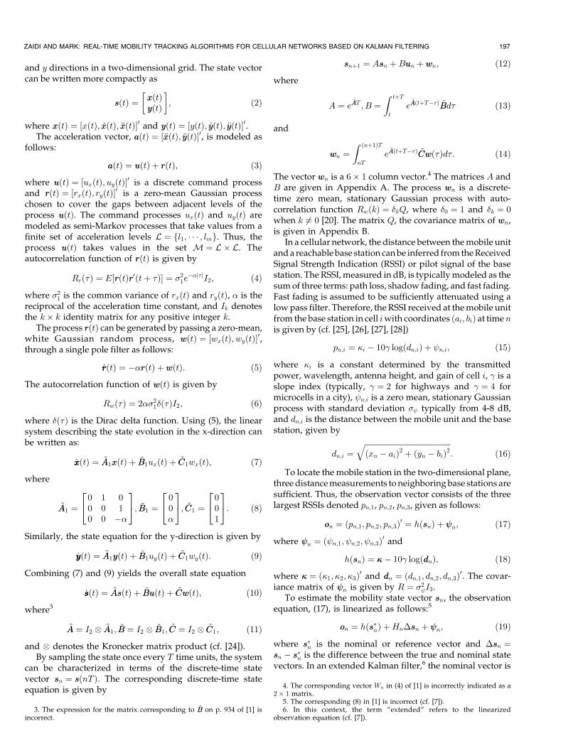
Fig. 1a illustrates the overall structure of our proposed MT-1

mobility estimator, consisting of a prefilter, a modified

Kalman filter, and an extended Kalman filter.

3.1.1 Prefilter

The prefilter consists of an averaging filter and a coarse

position estimator, as shown in Fig. 1b. The prefilter outputs

a vector of position estimates denoted by oooon ¼ ½xxn; yyn�0,which are used as the observation data for the modified

Kalman filter. The averaging filter reduces the shadowing

noise considerably, without significantly modifying the

path loss. The averaged RSSI measurements are then used

to generate coarse estimates of the position coordinates.The observation vector oon as given in (17) consists of the

path loss and the shadowing component. The averaging

filter reduces the shadowing component in the observa-

tions. Different filters can be used for this purpose.

Applying a rectangular window, the output ~oooon of the

averaging filter is given as

~oooon ¼ 1

N

Xni¼n�Nþ1

ooi; ð21Þ

whereN is the lengthof thewindow.For smallN , the residual

shadowing component is quite large and yields erroneous

position estimates; however, for large N , the path loss is

modified and induces errors in the position estimates. Our

solution to this problem is to use a bank of averaging filters in

series, each with small length N , instead of a single filter of

larger length. In the filter bank arrangement, each filter

performs an averaging operation according to (21) and

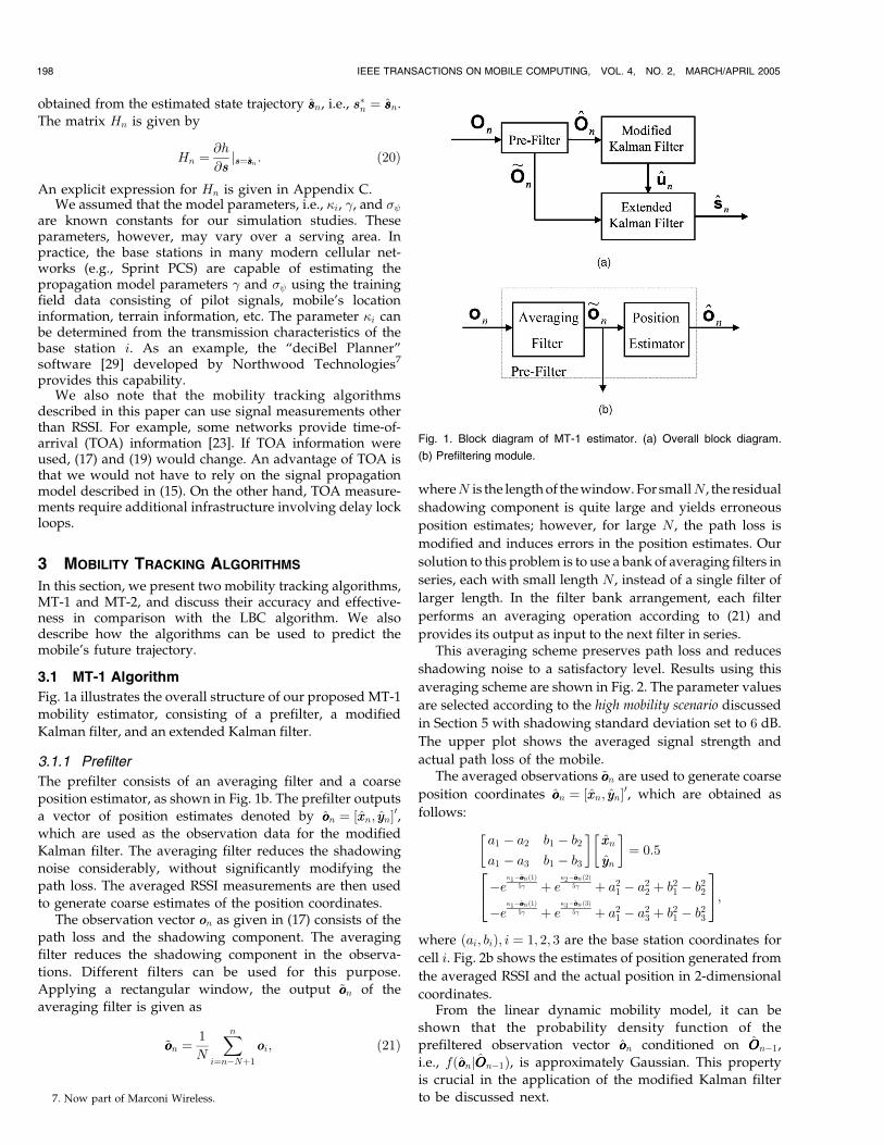
provides its output as input to the next filter in series.This averaging scheme preserves path loss and reduces

shadowing noise to a satisfactory level. Results using this

averaging scheme are shown in Fig. 2. The parameter values

are selected according to the high mobility scenario discussed

in Section 5 with shadowing standard deviation set to 6 dB.

The upper plot shows the averaged signal strength and

actual path loss of the mobile.The averaged observations ~oooon are used to generate coarse

position coordinates oooon ¼ ½xxn; yyn�0, which are obtained as

follows:

a1 � a2 b1 � b2

a1 � a3 b1 � b3

� �xxn

yyn

� �¼ 0:5

�e�1�~oooonð1Þ

5� þ e�2�~oooonð2Þ

5� þ a21 � a22 þ b21 � b22

�e�1�~oooonð1Þ

5� þ e�3�~oooonð3Þ

5� þ a21 � a23 þ b21 � b23

24

35;

where ðai; biÞ; i ¼ 1; 2; 3 are the base station coordinates for

cell i. Fig. 2b shows the estimates of position generated from

the averaged RSSI and the actual position in 2-dimensional

coordinates.From the linear dynamic mobility model, it can be

shown that the probability density function of the

prefiltered observation vector oooon conditioned on OOOOn�1,

i.e., fðoooonjOOOOn�1Þ, is approximately Gaussian. This property

is crucial in the application of the modified Kalman filter

to be discussed next.


Fig. 1. Block diagram of MT-1 estimator. (a) Overall block diagram.

(b) Prefiltering module.

7. Now part of Marconi Wireless.

3.1.2 Modified Kalman Filter

The conventional Kalman filter is modified to take intoaccount the discrete command process uun. A Bayesian-basedestimator for uun is integrated into the extendedKalman filter,resulting in the “modified Kalman filter” structure (cf. [1],[20], [21]). In the MT-1 estimator, it is important to note thatthe input to the modified Kalman filter is the vector ofprefiltered observations oooon, rather than the vector of rawobservations oon, as in the LBC algorithm [1].

In the MT-1 algorithm, the Bayesian-based estimator foruun is an approximation of the conditional mean of uun giventhe sequence, OOOOn ¼ ½oooo1; � � � ; oooon�0, of all prefiltered observa-tions up to time n:

uuuun ¼Xll2M

llPPfuun ¼ lljOOOOng; ð22Þ

where the conditional probability Pfuun ¼ lljOOOOng is approxi-

mated by

PPfuun ¼ lljOOOOng ¼ cfðoooonjuun ¼ ll; OOOOn�1ÞPPfuun ¼ lljOOOOn�1g; ð23Þ

with the constant c chosen such thatXjj2M

PPfuun ¼ jjjOOOOng ¼ 1:

The density fðoooonjuun ¼ ll; OOOOn�1Þ is approximatelyGaussian:

NðHpreðAssssn�1 þBllÞ; HpreMnjn�1H0preÞ; ð24Þ

where

Hpre ¼1 0 0 0 0 00 0 0 1 0 0

� �: ð25Þ

The approximate probability PPfuun ¼ lljOOOOn�1g can be calcu-

lated using the transition probability, all;jj, of the semi-

Markov process uun as follows:

PPfuun ¼ lljOOOOn�1g �Xjj2M

all;jjPfuun�1 ¼ jjjOOOOn�1g: ð26Þ

The probability estimates are initialized with the initial

discrete command state probabilities �ll ¼ Pfuu0 ¼ llg as

follows: PPfuu0 ¼ lljOOOO�1g ¼ �ll.

The modified Kalman filter is specified as follows: The

state estimate at time n is defined by ssssnjn ¼4 EðssnjOOOOnÞ, with

the initialization step ssss0j�1 ¼ 0, where 0 is the 6� 1 vector

of all zeros. The Kalman gain matrix is denoted by Kn. The

covariance matrix is defined by Mnjn�1 ¼4CovðssnjOOOOn�1Þ and

is initialized by M0j�1 ¼ I6.

Recursion steps for MT-1 modified Kalman filter (time n):

1. PPfuun ¼ lljOOOOn�1g ¼P

jj2M all;jjPfuun�1 ¼ jjjOOOOn�1g:2. PPfuun ¼ lljOOOOng ¼ cfðoooonjuun ¼ ll; OOOOn�1ÞPPfuun ¼ lljOOOOn�1g:3. uuuun ¼

Pll2M llPPfuun ¼ lljOOOOng:

4. Kn ¼Mnjn�1H0preðHpreMnjn�1H

0preÞ

�1:5. ssssnjn ¼ ssssnjn�1 þKnðoooon �Hpressssnjn�1Þ[Correction step].6. ssssnþ1jn ¼ Assssnjn þBuuuun [Prediction step].


Fig. 2. Performance of prefilter in MT-1 algorithm.

7. Mnjn ¼ ðI �KnHpreÞMnjn�1ðI �KnHpreÞ0:8. Mnþ1jn ¼ AMnjnA

0 þQ:

In the recursion part of the filter, the first three steps

correspond to the Bayesian-based estimator and the

remaining steps implement a conventional Kalman filter.

3.1.3 Extended Kalman Filter

The modified Kalman filter described above provides the

mobility state estimates ssssnjn and discrete command esti-

mates uuuun. However, the accuracy of the mobility state

estimates ssssnjn is largely dependent on the performance of

the prefilter. Since the coarse position estimates are used as

the observations for the modified Kalman filter, the best the

filter can do is to track the coarse position coordinates. Any

inaccuracy and error in the prefilter can cause the estimator

to diverge.To avoid this problem, we have introduced a second

(extended) Kalman filter to produce the mobility state

estimates. The extended Kalman filter, as shown in Fig. 1a,

takes the averaged pilot signal strengths OOOOn as observations

and the estimated discrete command states uuuun from the

modified Kalman filter and generates the mobility state

estimate ssssnjn. The extended Kalman filter consists of a

recursion similar to that of Section 3.1.2 (cf. [7]).

Recursion steps for MT-1 extended Kalman filter (time n):

1. Hn ¼ @h@ss ss¼ssssnjn�1

�� :2. Kn ¼Mnjn�1H

0nðHnMnjn�1H

0n þRresÞ�1:

3. ssssnjn ¼ ssssnjn�1 þKnð~oooon � hðssssnjn�1ÞÞ[Correction step].4. ssssnþ1jn ¼ Assssnjn þBuuuun [Prediction step].5. Mnjn ¼ ðI �KnHnÞMnjn�1ðI �KnHnÞ0 �KnRresK

0n:

6. Mnþ1jn ¼ AMnjnA0 þQ:

The matrix Rres is used in the Kalman filter recursion as

the covariance matrix of the residual noise in the averaged

RSSI’s. A suitable matrix for Rres is �I3, where � � 0:01. The

overall performance of the MT-1 mobility estimator in

Fig. 1a does not depend strongly on the performance of the

prefilter since the residual noise of the prefilter is removed

by the extended Kalman filter.

3.2 MT-2 Algorithm

As discussed before, the prefilter used in the MT-1 mobility

estimation scheme requires a relatively high frequency of

pilot signal samples to be received from the same base

station, i.e., one sample per time slot, in order for the

averaging filter to reduce the shadowing noise sufficiently.

In real-time wireless systems, it is not always possible to

meet this requirement on the observation data. At times, it

is difficult to obtain a collection of measurements from the

same base station because the mobile may move out of

range from the base station or an obstruction might make

the corresponding signal difficult to measure accurately.We have developed the MT-2 algorithm as an alternative

estimation scheme to deal with scenarios where the prefilter

cannot be used to obtain coarse position estimates effec-

tively (cf. Section 3.1.1). Under such scenarios, the discrete

command process cannot be estimated accurately by the

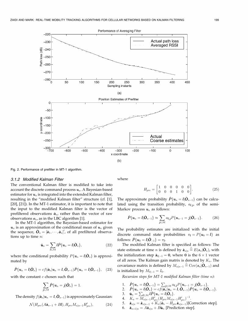
MT-1 algorithm. As shown in Fig. 3, the MT-2 algorithm

consists of a single extended Kalman filter and the discrete

command process is treated as additional noise. Here, thetotal noise covariance matrix is given by

~QQ ¼ QþBE½ðuun �E½uun�Þðuun � E½uun�Þ0�B0; ð27Þ

where the matrix Q, the covariance matrix of wwn, is given inAppendix B. The discrete command process uun consists oftwo zero-mean independent semi-Markov processes, so thecovariance matrix of uun is given by

E½ðuun �E½uun�Þðuun �E½uun�Þ0� ¼ �2uI2; ð28Þ

where �2u is the variance of ux and uy. Although the noiseprocess in this case, i.e., Buun þ wwn, is not white noise, weignore the correlation between the noise samples.

The recursion steps in the extended Kalman filter of Fig. 3are similar to that of the extended Kalman filter described inSection 3.1.3 and are given as follows:

Recursion steps for MT-2 extended Kalman filter (time n):

1. Hn ¼ @h@ss ss¼ssssnjn�1

�� :2. Kn ¼Mnjn�1H

0nðHnMnjn�1H

0n þRÞ�1:

3. ssssnjn ¼ ssssnjn�1 þKnðoon � hðssssnjn�1ÞÞ[Correction step].4. ssssnþ1jn ¼ Assssnjn [Prediction step].5. Mnjn ¼ ðI �KnHnÞMnjn�1ðI �KnHnÞ0 �KnRK

0n:

6. Mnþ1jn ¼ AMnjnA0 þ ~QQ:

3.3 Comparison with LBC Algorithm

The LBC estimator proposed in [1] consists only of the

modifiedKalman filter,which takes the rawobservation data

as input and produces mobility state estimates. In this case,

the Bayesian-based estimator in the modified Kalman filter

approximates the conditional probability density of the pilot

signal strengths given the vector of previous observations

OOn�1 with a Gaussian density, i.e., NðHnðAssssn�1 þBuuuun�1Þ;HnMnjn�1H

0n þRÞ (cf. (43) of [1]). The matrix Mnjn�1 ¼

4

CovðssnjOOn�1Þ is the covariancematrix and the transformation

matrix Hn is given in (20). This assumption turns out to be

inaccurate and can lead to divergence of the LBC estimator.

An approximation for the conditional probability density

function of each element of the observation vector, i.e., the

pilot signal strengths pn;i, conditioned on the past observa-

tions is given in Appendix D.In our numerical studies (see Section 5), we have found

that the Bayesian-based estimator can give inaccurateestimates of uun, primarily due to the approximation of thedensity fðoonjOOn�1Þ by a Gaussian density. The inaccuracy inthe estimates uuuun leads to divergence of the modifiedKalman filter. Consequently, the LBC estimator is not ableto track a mobile station that undergoes sudden changes inacceleration. To solve this inherent problem of the LBCestimator, the MT-1 algorithm preprocesses the RSSImeasurements using the prefilter to extract the observationssuitable for the modified Kalman filter. In MT-1, themodified Kalman filter from the LBC scheme is retained,


Fig. 3. Block diagram for MT-2 estimator.

but its input consists of coarse position estimates from theprefilter, rather than the raw RSSI measurements. Further-more, in the MT-1 algorithm, the modified Kalman filter isused only to generate estimates of the discrete commandprocess and a second (extended) Kalman filter is used toyield mobility state estimates using the discrete commandestimates and averaged RSSI measurements as inputs. Thecombination of two Kalman filters in the MT-1 estimatorperforms much better than the LBC estimator.

In the MT-2 algorithm, the discrete command process uunis not estimated explicitly, but is treated as additional noise.The structure of the MT-2 estimator is simpler than that ofthe LBC estimator because it does not include the Bayesian-based estimator for the discrete command process. Thus,the MT-2 algorithm avoids the inherent inaccuracy of theBayesian-based estimator used in the LBC algorithm. Ournumerical results (cf. Section 5) show that MT-2 consistentlyoutperforms the LBC algorithm.

3.4 Mobility Prediction

Under the dynamic mobility model discussed in Section 2,knowledge of the mobility state information at a given timet0 allows us to predict the mobility state at a time t in thefuture. The predicted state ~sssst of a mobile node at time t isgiven as follows, assuming that the state estimate sssst0 at timet0 is available:

~sssst ¼ Aðt� t0Þsssst0 ; ð29Þ

where Aðt� t0Þ ¼ I2 �A1ðt� t0Þ. The matrix A1 is given in(32). The error covariance matrix Mt�t0 for the predictedmobility state is given by

Mt�t0 ¼ Aðt� t0ÞMt0Aðt� t0Þ0 þ �2uBðt� t0ÞBðt� t0Þ0þQðt� t0Þ; ð30Þ

whereMt0 ¼ Covðsssst0Þ,�2u is thevariance ofux anduy,Bðt� t0Þ¼ I2 �B1ðt� t0Þ, and Qðt� t0Þ ¼ 2��21I2 �Q1ðt� t0Þ. Thematrices B1 and Q1 are given in (32) and (33).

Mobility prediction can play a key role in advancedresource management schemes that anticipate the futureresource needs of a mobile station. Some promisingapplications include smooth handoff [1] and fast wirelessInternet service provisioning [5]. It is important to note thatin using the mobility prediction information (29), one musttake into account the degree to which the prediction errorgrows with time, as indicated by (30).

4 MOBILITY STATE OBSERVABILITY

As discussed before, three measurements of pilot signals areneeded to locate themobile unit in two-dimensional space. Inreal systems, it is not always possible for themobile to obtainsignal measurements from three independent base stations.At times, the mobile may not be able to obtain accuratemeasurements from at least three pilots as the signals comingfrom farther base stations may become very weak. In theestimation scheme of Liu et al. [1], the observation set at eachsampling instant is assumed to consist of independent RSSImeasurements from three different base stations. However,by considering the observability properties of the mobilitymodel,weshall showthatmobility trackingcanbeperformedwith fewer than three independent RSSI measurements. It iswell-known that the Kalman filter can yield meaningful

estimates of the system state only if the underlying system isobservable [30].

Since the RSSI measurements are nonlinear functions ofthe mobility state as given in (17), the Jacobian of thetransformation function hðssnÞ, i.e., Hn (cf. (20) andAppendix C) is used to determine observability of thesystem. The system of (12) is observable over the interval½n0; n1� if and only if the columns of the matrix OobsðnÞ ¼Hn�ðn0; nÞ are linearly independent functions of n over½n0; n1�, where �ðn0; nÞ is the state-transition matrix of thesystem (cf. [31]). For the discrete-time realization of thesystem (cf. (12)), the matrix �ðn0; nÞ ¼ An�n0 , where A isgiven in Appendix A. By examining the structure of theobservability matrix OobsðnÞ ¼ HnA

n�n0 , as given in Appen-dix E, the system observability can be characterized moresimply as follows:

Proposition 1. The system of (12) is observable over the interval½n0; n1� if and only if xxðnÞ 6¼ cyyðnÞ for each n over ½n0; n1�,where c is a constant, xxðnÞ ¼ ðxn � a1; xn � a2; xn � a3Þ, andyyðnÞ ¼ ðyn � b1; yn � b2; yn � b3Þ.

Proposition 1 implies that the system is observableunder fairly general conditions when three independentRSSI measurements are available at each time slot, asshould be expected from geometric considerations. Whenonly two RSSI measurements per time slot are available,say from base stations 1 and 2, the observability conditionreduces to the inequality of the vectors ðxn � a1; xn � a2Þand cðyn � b1; yn � b2Þ as functions of n over the interval½n0; n1�. Therefore, in principle, two independent RSSImeasurements per time slot can be sufficient for mobilitytracking. Similarly, with only one RSSI measurement, sayfrom base station 1, the observability condition reduces tothe inequality of the functions ðxn � a1Þ and cðyn � b1Þ overthe interval ½n0; n1�. In this case, if the movement of themobile remains linear for the length of the interval ½n0; n1�,then the observability condition is not satisfied, i.e.,ðxn � a1Þ ¼ cðyn � b1Þ, and estimates of the mobility statescannot be found.

We remark that collecting observations beyond a certaintime window has a negligible effect on the observability ofthe system. The bound on the effective observation windowis due to the characteristics of the linear dynamic systemmodel of user’s mobility. In this model, the autocorrelationbetween the random acceleration of the mobile station attime t and tþ � decays exponentially as � increases(cf. Section 2). This decay depends on the time-coefficientof acceleration �, with larger � implying faster decay. FromAppendix E, one can see that the effect of larger � is toreduce the effective observation window, as subsequentobservations beyond the window become less relevant tomobility state estimation at the initial time n0.

Of course, besides the observability criterion of Proposi-tion 1, there are other factors involved in determining theeffectiveness of the mobility tracking. In general, theestimation error is reduced when more independentobservations are available. Our numerical results (seeSection 5) show that the simplified mobility trackingalgorithm MT-2 performs well even when only twoindependent RSSI measurements are available.


5 NUMERICAL RESULTS

In our numerical experiments, random mobile trajectoriesare generated in Matlab using the dynamic state modelgiven in (12). The position coordinates are specified in unitsof meters. The parameters determining the autocorrelationfunction of the random acceleration process rrðtÞ are set asfollows (cf. (4)): � ¼ 1000 s�1 and �1 ¼ 1 dB. The covariancematrix R of n (cf. (17)) is determined by setting theparameter � ¼ 6 dB. The state vector ssðtÞ is initialized tothe zero vector.

The discrete command processes uxðtÞ and uyðtÞ areindependent semi-Markov processes, each taking on fivepossible levels of acceleration comprising the set L ¼ f�5,�2:5, 0, 2:5, 5g in units ofm=s2. This set of acceleration levels iscapable of generating a wide range of dynamic motion. Werefer to this selectionas thehighmobility scenario.Thesamplinginterval is set to T ¼ 0:1s. The initial probability vector �� fortheHSMM is initialized to the uniformdistribution. The totalduration of each sample trajectory isN ¼ 600 sample points,which corresponds to 2 minutes. The elements of thetransition probability matrix Ah are initialized to a commonvalue of 1=5. We assume that the dwell times in each state areuniformly distributed with a commonmean value of 2 s. Theparameter �i is assumed to be zero for all cells i.

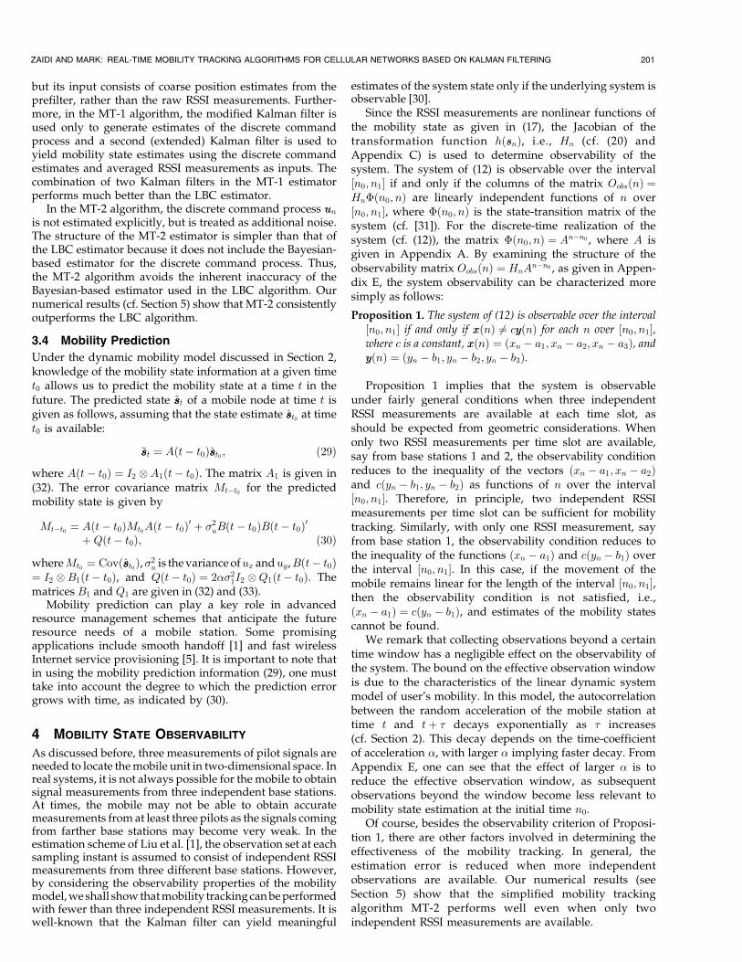
Fig. 4 shows a typical sample mobile trajectory,8 gener-ated by the dynamic state model with the given parametervalues. The figure also shows estimated trajectories obtainedfrom the LBC algorithm and the MT-1 algorithm, respec-tively. The figure shows that the LBC algorithm fails to trackthe actual trajectory, particularly when there are sharp orsudden changes in direction. We remark that standard GPStechniques would also fail to track the sudden accelerationsproduced by the dynamic state model with the givenparameter settings. On the other hand, MT-1 is able to followthe curves of the actual trajectory with reasonably good

accuracy.We remark that the sample trajectories correspond-ing to the specified parameter values are considerably moredynamic than those of an actual mobile station in a livenetwork environment. They provide a good benchmark toevaluate the robustness and accuracy of mobility trackingalgorithms.

We use root mean squared error (RMSE) as a figure ofmerit to compare a given trajectory fxn; yng and itsestimated trajectory fxxn; yyng:

RMSE ¼

ffiffiffiffiffiffiffiffiffiffiffiffiffiffiffiffiffiffiffiffiffiffiffiffiffiffiffiffiffiffiffiffiffiffiffiffiffiffiffiffiffiffiffiffiffiffiffiffiffiffiffiffiffiffiffiffiffiffiffiffiffiffiffi1

N

XNn¼1

½ðxxn � xnÞ2 þ ðyyn � ynÞ2�

vuut : ð31Þ

Table 1 shows the sample mean and variance of the RMSEstatistic computed using more than 500 independentlygenerated sample trajectories. We denote the selection ofacceleration levels between�5 to 5 m=s2 as the high mobilityscenario in Table 1. To evaluate the comparative perfor-mance of MT-1 and MT-2 with LBC under low mobilityconditions more typical for actual cellular networks, we alsoperform a set of simulations for the discrete command levelsselected fromL ¼ f�0:5;�0:25; 0; 0:25; 0:5gm=s2. The respec-tive results are listed under the “low mobility scenario”column in Table 1. In the scenarios of Table 1, three basestations provide independent RSSI measurements at eachtime slot. The performance of the mobility tracking algo-rithms is evaluatedwhen the parameter � is set to 6 dB and 8dB. Recall that � determines the covariance matrix of theobservation noise (cf. (17)).

Table 1 provides a quantitative comparison of the relativemerits of the MT-1, MT-2, and LBC estimators, whichconfirms the qualitative implications of Fig. 4. The tableshows that under perfect observation conditions for prefilter-ing, the MT-1 estimator achieves the best performance. TheMT-2 estimator performs reasonably well and clearly out-performs theLBCestimator. Theperformancedegradation ofthe LBC estimator is observed to bemuch greater than that of


8. The starting point is at ð0; 0Þ.

Fig. 4. Performance of MT-1 and LBC algorithms.

MT-1andMT-2when thenoise level in theobservationdata isincreased.

Table 1 also shows performance degradation for the LBCestimator when the trajectories are more dynamic althoughthe other tracking algorithms show stable or even betterperformance for the highmobility scenario. In our numericalanalysis, we also performed simulations for the lowermobility conditions andMT-1 andMT-2 consistentlyperformbetter than LBC. We conclude that MT-1 and MT-2 achievebetter performance than LBC over a wide range of mobilityscenarios and wireless propagation environments.

Table 1 also provides a quantitative performancecomparison of MT-1 and MT-2 with the sequential MonteCarlo (SMC) approach to mobility tracking (cf. [2]). Thenumber of samples is selected to be 800 corresponding tothe best estimator described in [2]. The initial mobility statesamples are initialized as zero vectors and their respectiveweights are initialized to unity. Table 1 shows that althoughSMC provides better performance than LBC, the MT-1 and

MT-2 estimators both outperform the SMC estimator for alltested scenarios of mobility and propagation environments.The MT-1 and MT-2 estimators are also computationallysimpler than the SMC algorithm.

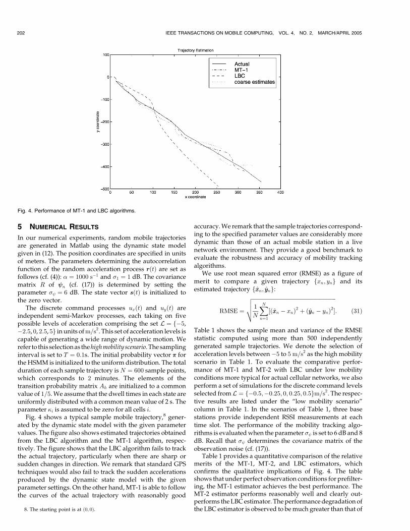
Fig. 5 shows a sample trajectory of a mobile user in acellular network, along with the estimated and predictedtrajectories under the MT-1 algorithm. The predictedtrajectory is a straight line that starts in the upper right-hand corner of the figure at the point ð�125;�85Þ. Observethat the predicted trajectory initially stays close to theestimated trajectory and then deviates from it over time.The deviation indicates the increase in prediction error or,more precisely, the prediction uncertainty. An importantpoint to be noted here is that although prediction errorincreases with time, the estimation error is independent oftime once the Kalman filter reaches the steady state.

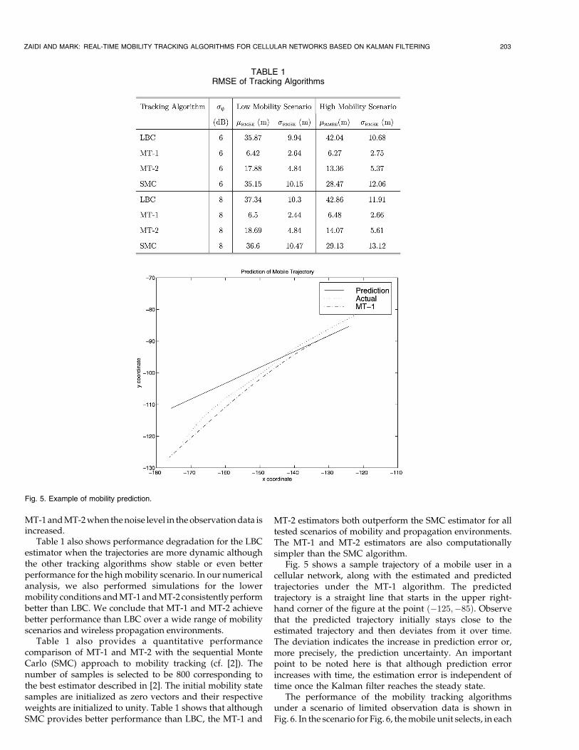
The performance of the mobility tracking algorithmsunder a scenario of limited observation data is shown inFig. 6. In the scenario for Fig. 6, themobile unit selects, in each


TABLE 1RMSE of Tracking Algorithms

Fig. 5. Example of mobility prediction.

time slot, three RSSI measurements from a set of nine base

stations in its vicinity to forman active set. Inpractice, the three

strongest RSSI measurements would be selected. In order tosimulate the effect of the dynamic changes to the active set of

three base stations over time, the active set changes from time

slot to time slot in the sequence f1; 2; 3g, f4; 5; 6g, f7; 8; 9g, andrepeats. Thus, anRSSImeasurement fromagivenbase station

is available onlyonce every three time slots. This scenariowaschosen to reflect similar patterns observed in test drives of an

actualCDMAnetwork.As can be seen in Fig. 6, only theMT-2

algorithm is able to track the mobile trajectory accurately. In

this case, the prefilter in the MT-1 algorithm is ineffective,

resulting in inaccurate discrete command estimates. In the

LBC algorithm, the discrete command estimates are alsoinaccurate, although for a different reason (cf. Section 3.3).

In Fig. 7a, a sample trajectory is estimated using the MT-2

algorithmfor the followingdifferent casesof observationdata

availability:

. w 1 obs, 1 BS: One RSSI measurement per time slotfrom one base station.

. w 1 obs, 2 BS: One RSSI measurement per time slotalternately from two base stations.

. w 2 obs: Two independent RSSI measurements pertime slot.

. w 3 obs: Three independent RSSI measurements pertime slot.

The initial position of the sample trajectory of Fig. 7a isshown by “*” whereas the estimated trajectories areinitialized at the origin. When three independent RSSImeasurements are available per time slot, the MT-2estimator converges fastest to the true trajectory. Whentwo RSSI measurements are available per time slot, con-vergence occurs more slowly. The worst case shown is whenonly one observation from a single base station is availablethroughout the course of trajectory estimation. In this case,the MT-2 estimator fails to track the given trajectory.

An explanation of this last case in terms of the observa-bility arguments of Section 4 is given as follows: Since � ¼1000 s�1 and T ¼ 0:1 s, the observation window is approxi-mately 5, i.e., 0.5 seconds (see Appendix E). During this shorttime window, the movement of the mobile remainsapproximately linear and, consequently, the system is notobservable (cf. Section 4). However, the estimation perfor-mance improves significantly if two base stations supply oneobservation per sampling interval alternately. Thus, invol-ving RSSI measurements from another base station helps tosatisfy the observability criterion.

For the cases where fewer than three observations areavailable, the estimation performance is largely determinedby the observability criteria. The estimators are not depend-able for the intervals when the system is unobservable. Also,more observations provide more redundancy to overcomethe observation noise. In the case where three observationsare available, the estimator performs equally well regardlessof whether or not prior knowledge of the mobile (i.e., initiallocation) is known.

In Fig. 7b, the performance of MT-2 is shown for differentnumbers of observations available at each sampling instantwhen some prior knowledge of the initial position of themobile unit is given. This situation may occur when, forexample, the number of independent RSSI measurementssuddenly reduces from three to two and the most recentposition estimate effectively initializes the future iterationsof the tracking algorithm on the reduced observation dataset. In practice, pilot signals from one or more of the basestations in the active set may become corrupted due to pathobstructions during a call and, hence, the active set may haveto be reduced in size. With prior knowledge of the mobile’sposition, the availability of two independent RSSI measure-ments yields similar performance as in the case with threeindependent RSSI measurements. When only one observa-tion is available in alternate time slots from two basestations, we observe a reduction in tracking performance. As


Fig. 6. Performance of mobility tracking algorithms under limited observation data.

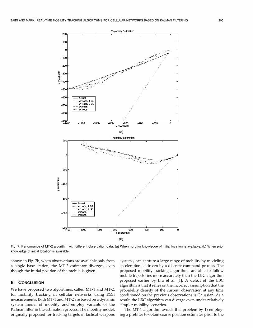
shown in Fig. 7b, when observations are available only from

a single base station, the MT-2 estimator diverges, even

though the initial position of the mobile is given.

6 CONCLUSION

We have proposed two algorithms, called MT-1 and MT-2,

for mobility tracking in cellular networks using RSSI

measurements. BothMT-1 andMT-2 are based on a dynamic

system model of mobility and employ variants of the

Kalman filter in the estimation process. The mobility model,

originally proposed for tracking targets in tactical weapons

systems, can capture a large range of mobility by modelingacceleration as driven by a discrete command process. Theproposed mobility tracking algorithms are able to followmobile trajectories more accurately than the LBC algorithmproposed earlier by Liu et al. [1]. A defect of the LBCalgorithm is that it relies on the incorrect assumption that theprobability density of the current observation at any timeconditioned on the previous observations is Gaussian. As aresult, the LBC algorithm can diverge even under relativelysimpler mobility scenarios.

The MT-1 algorithm avoids this problem by 1) employ-ing a prefilter to obtain coarse position estimates prior to the


Fig. 7. Performance of MT-2 algorithm with different observation data. (a) When no prior knowledge of initial location is available. (b) When prior

knowledge of initial location is available.

application of the modified Kalman filter and 2) decoupling

mobility state estimation from estimation of the discrete

command process. The MT-2 algorithm consists of a single

extended Kalman filter, wherein the discrete command

process is treated as additional noise. Under certain

scenarios of limited observation data where MT-1 fails,

MT-2 is able to track mobility with adequate accuracy. In all

of our numerical experiments, both MT-1 and MT-2

outperform the LBC algorithm by a large margin. The

MT-1,2 algorithms also compare favorably against the SMC

mobility tracking algorithm proposed in [2].Requirements on the observation data for the tracking

algorithms were also investigated and observability argu-

ments from systems theory suggested that mobility tracking

could be achieved with fewer than three independent RSSI

measurements from base stations. Our numerical results

showed that two independent RSSI measurements were

sufficient for mobility tracking but a single RSSI measure-

mentwasnot. Theproposedmobility tracking algorithms can

be used in mobility-based resource allocation schemes such

as fast IPhandoff [3] andprecaching ofWebproxy servers [5].

APPENDIX A

STATE EQUATION MATRICES

The matrices A and B are given by:9

A ¼ e~AAT ;B ¼

Z tþT

t

e~AAðtþT��Þ ~BBd�:

Using standard techniques from matrix algebra, the

matrices can be written as

A ¼ I2 �A1ðT Þ; B ¼ I2 �B1ðT Þ;

where

A1ðT Þ ¼1 T a0 1 b0 0 e��T

24

35; B1ðT Þ ¼

c�a�b

24

35; ð32Þ

and

a ¼ ð�1þ �T þ e��T Þ=�2;

b ¼ ð1� e��T Þ=�;

c ¼ ð1� �T þ �2

2T 2 � e��T Þ=�2:

APPENDIX B

COVARIANCE MATRIX OF DISCRETE WHITE NOISE

The matrix Q is given by10

Q ¼ 2��21I2 �Q1ðT Þ;

where Q1ðT Þ ¼ ½qij� is a symmetric 3� 3 matrix with upper

triangular entries given as follows:

q11 ¼ ð1� e�2�T þ 2�T þ 2�3T 3=3� 2�2T 2 � 4�Te��T Þ=ð2�5Þ;

q12 ¼ ðe�2�T þ 1� 2e��T þ 2�Te��T � 2�T þ �2T 2Þ=ð2�4Þ;q13 ¼ ð1� e�2�T � 2�Te��T Þ=ð2�3Þ;q22 ¼ ð4e��T � 3� e�2�T þ 2�T Þ=ð2�3Þ;q23 ¼ ðe�2�T þ 1� 2e��T Þ=ð2�2Þ;q33 ¼ ð1� e�2�T Þ=ð2�Þ:

ð33Þ

APPENDIX C

TRANSFORMATION MATRIX OF LINEARIZEDOBSERVATIONS

The matrix Hn in the linearized observation (19) is given by

Hn ¼ �5�hhn;1hhn;2hhn;3

24

35;

where hhn;i is the ith row of Hn with

hhn;i ¼2

d2n;iðxn � ai; 0; 0; yn � bi; 0; 0Þ;

for i ¼ 1; 2; 3.

APPENDIX D

PROBABILITY DENSITY FUNCTION OF RSSI

The conditional probability density function (pdf) of the

mobility state vector conditioned on the past observations is

approximately Gaussian (cf. [1]), i.e.,

fðssnjOOn�1Þ � N ðAssssn�1 þBuuuun�1;Mnjn�1Þ; ð34Þ

where OOn�1 ¼ ðoon�1; ::::; oo1Þ and the matrix Mnjn�1 ¼4

CovðssnjOOn�1Þ is the covariance matrix. Thus, the position

coordinates of the mobile ðxn; ynÞ conditioned on OOn�1 can

be approximated by Gaussian random variables with (mean,

variance) given by ðx; �2xÞ and ðy; �2yÞ, respectively. Thesequantities can be obtained from the mean and covariance

matrices of the mobility state vector as defined in (34). The

pdf of the distance, dn;i, of the mobile from a base station in

cell i at sampling time n is given by

fdn;iðÞ ¼

2��x�ygðÞ;

where

gðÞ ¼4Z 2�

0

exp

� cos �� ðx � aiÞð Þ2

2�2x�

sin �� ðy � biÞ� �2

2�2y

!d�;

and ðai; biÞ are the coordinates of base station i. The path

loss for cell i is hi ¼ �i � 10� logðdn;iÞ, where the pdf of hi is

given by


9. The expression for the matrix B given in (36) of [1] is incorrect.10. This expression is equivalent to (37) in [1].

fhið�Þ ¼1

20��x�ye�i��5� g e

�i��10�

� �:

The conditional pdf of the pilot signal strength pn;i given

the previous observations is approximated by

fpn;ið jOOn�1Þ ¼1

20��x�y

1ffiffiffiffiffiffiffiffiffiffiffi2��2

q Z 1

�1e�i��5� e

�ð ��Þ2

2�2 g e

�i��10�

� �d�:

The above expression cannot be evaluated in closed form.

Numerical integration might be a possible solution, but is

time-consuming and, therefore, unsuitable for real-time

mobility estimation.

APPENDIX E

OBSERVABILITY MATRIX

The observabilitymatrixOobsðnÞ ¼ HnAn�n0 can bewritten as

OobsðnÞ ¼ �10�½Oobs;xðnÞ; Oobs;yðnÞ�; ð35Þ

where

Oobs;xðnÞ ¼px;1 px;1ðn� n0ÞT px;1pnpx;2 px;2ðn� n0ÞT px;2pnpx;3 px;3ðn� n0ÞT px;3pn

24

35 ð36Þ

and Oobs;yðnÞ is defined similarly, except that the subscript x

is replaced by y. Here,

px;i ¼xn � aid2n;i

; py;i ¼yn � bid2n;i

; i ¼ 1; 2; 3;

and

pn ¼ 1

�2�1þ ðn� n0Þ�T þ e�ðn�n0Þ�T� �

:

We remove the constant �10� in (35) and perform the

following column operations on OobsðnÞ, where Ci denotes

the ith column:

1. C3 ¼ �2C3 and C6 ¼ �2C6, and2. C3 ¼ C3 þ C1 � �C2 and C6 ¼ C6 þ C4 � �C5

to obtain a reduced matrix ~OOobsðnÞ ¼ ½ ~OOobs;xðnÞ; ~OOobs;yðnÞ�,where

~OOobs;xðnÞ ¼px;1 px;1ðn� n0ÞT px;1e

�ðn�n0Þ�T

px;2 px;2ðn� n0ÞT px;2e�ðn�n0Þ�T

px;3 px;3ðn� n0ÞT px;3e�ðn�n0Þ�T

24

35 ð37Þ

and ~OOobs;yðnÞ is defined similarly.Note that the third and sixth columns of ~OOobsðnÞ consist

of exponentials which go to zero as ðn� n0Þ increases. Thisimplies a limit on the effective observation window size. For

example, if � ¼ 1000 s�1 and T ¼ 0:1 s, then e�ðn�n0Þ�T � 0

for ðn� n0Þ ¼ 5, which implies that only the first five

observations from n0 are useful for estimating the system

state at time n0.From (37), one sees that observability of the system, or

the linear independence of columns of ~OOobsðnÞ over an

observation interval ½n0; n1�, depends on the position

coordinates ðxn; ynÞ of the mobile. The system is observable

over the interval ½n0; n1� if and only if xxðnÞ 6¼ cyyðnÞ for each

n over ½n0; n1], where c is a constant and xxðnÞ and yyðnÞ arethe vector functions xxðnÞ ¼ ðxn � a1; xn � a2; xn � a3Þ and

yyðnÞ ¼ ðyn � b1; yn � b2; yn � b3Þ.

ACKNOWLEDGMENTS

This work was supported by the US National Science

Foundation under Grant No. ACI-0133390 and by a grant

from the TRW Foundation.

REFERENCES

[1] T. Liu, P. Bahl, and I. Chlamtac, “Mobility Modeling, LocationTracking, and Trajectory Prediction in Wireless ATM Networks,”IEEE J. Selected Areas in Comm., vol. 16, pp. 922-936, Aug. 1998.

[2] Z. Yang and X. Wang, “Joint Mobility Tracking and Hard Handoffin Cellular Networks via Sequential Monte Carlo Filtering,” Proc.IEEE INFOCOM ’02, vol. 2, pp. 968-975, June 2002.

[3] J. Kempf, J. Wood, and G. Fu, “Fast Mobile IPv6 Handover PacketLoss Performance,” Proc. IEEE Wireless Networking and Comm.Conf. (WCNC ’03), Mar. 2003.

[4] Y. Gwon, G. Fu, and R. Jain, “Fast Handoffs in Wireless LANNetworks Using Mobile Initiated Tunneling Handoff Protocol forIPv4 (MITHv4),” Proc. IEEE Wireless Networking and Comm. Conf.(WCNC 2003), pp. 1248-1252, Mar. 2003.

[5] H. Kobayashi, S.Z. Yu, and B.L. Mark, “An Integrated Mobilityand Traffic Model for Resource Allocation in Wireless Networks,”Proc. Third ACM Int’l Workshop Wireless Mobile Multimedia, pp. 39-47, Aug. 2000.

[6] J.B. Tsui, Fundamentals of Global Positioning System Receivers: ASoftware Approach. New York: John Wiley & Sons, 2000.

[7] R.G. Brown and P.Y. Hwang, Introduction to Random Signals andApplied Kalman Filtering. third ed., New York: John Wiley & Sons,1997.

[8] G.M. Djuknic and R.E. Richton, “Geo-Location and Assisted GPS,”Computer, vol. 34. pp. 123-125, Feb. 2001.

[9] F.V. Diggelen, “Indoor GPS Theory and Implementation,” Proc.IEEE Position Location and Navigation Symp. 2002, pp. 240-247, 2002.

[10] K.C. Ho and Y.T. Chan, “Solution and Performance Analysis ofGeolocation by TDOA,” IEEE Trans. Aerospace and ElectronicSystems, pp. 1311-1322, Oct. 1993.

[11] P. Deng and P.Z. Fan, “An AOA Assisted TOA PositioningSystem,” Proc. World Computer Congress-Int’l Conf. CommunicationTechnology (WCC-ICCT ’00), vol. 2, pp. 1501-1504, 2000.

[12] L. Cong and W. Zhuang, “Hybrid TDOA/AOA Mobile UserLocation for Wideband CDMA Cellular Systems,” IEEE Trans.Wireless Comm., vol. 1, pp. 1439-1447, July 2002.

[13] P. Bahl and V.N. Padmanabhan, “RADAR: An In-Building RF-Based User Location and Tracking System,” Proc. IEEE INFOCOM’00, vol. 2, pp. 775-784, Mar. 2000.

[14] P.C. Chen, “A Cellular Based Mobile Location Tracking System,”Proc. IEEE Vehicular Technology Conf. (VTC ’99), pp. 1979-1983,1999.

[15] D. Gu and S.S. Rappaport, “A Dynamic Location TrackingStrategy for Mobile Communication Systems,” Proc. VehicularTechnology Conf. (VTC ’98), pp. 259-263, 1998.

[16] Y. Lin and P. Lin, “Performance Modeling of Location TrackingSystems,” Mobile Computing and Comm. Rev., vol. 2, no. 3, pp. 24-27, 1998.

[17] M. Hellebrandt and R. Mathar, “Location Tracking of Mobiles inCellular Radio Networks,” IEEE Trans. Vehicular Technology,vol. 48, pp. 1558-1562, Sept. 1999.

[18] I.F. Akyildiz, Y.B. Lin, W.R. Lai, and R.J. Chen, “A New RandomWalk Model for PCS Networks,” IEEE J. Selected Areas in Comm.,vol. 18, no. 7, pp. 1254-1260, 2000.

[19] K.K. Leung, W.A. Massey, and W. Whitt, “Traffic Models forWireless Communication Networks,” IEEE J. Select. Areas inComm., vol. 12, pp. 1353-1364, Oct. 1994.

[20] R.A. Singer, “Estimating Optimal Tracking Filter Performance forManned Maneuvering Targets,” IEEE Trans. Aerospace andElectronic Systems, vol. 6, pp. 473-483, July 1970.

[21] R.L. Moose, H.F. Vanlandingham, and D.H. McCabe, “Modelingand Estimation for Tracking Maneuvering Targets,” IEEE Trans.Aerospace and Electronic Systems, vol. 15, pp. 448-456, May 1979.


[22] B.L. Mark and Z.R. Zaidi, “Robust Mobility Tracking for CellularNetworks,” Proc. IEEE Int’l Conf. Comm. (ICC ’02), vol. 1, pp. 445-449, May 2002.

[23] J.J. Caffery Jr., Wireless Location in CDMA Cellular Radio Systems.Norwell, Mass.: Kluwer Academic, 1999.

[24] R.E. Bellman, Introduction to Matrix Analysis. New York: McGraw-Hill, 2nd ed. 1970.

[25] G.L. Stuber, Principles of Mobile Communication. second ed., Mass.:Kluwer Academic, 2001.

[26] M. Gudmundson, “Correlation Model for Shadowing Fading inMobile Radio Systems,” Electronic Letters, vol. 27, pp. 2145-2146,Nov. 1991.

[27] H. Suzuki, “A Statistical Model for Radio Propagation,” IEEETrans. Comm., vol. 25, pp. 673-680, July 1977.

[28] J.W. Mark and W. Zhuang, Wireless Communications and Network-ing. Prentice Hall, 2003.

[29] DeciBel Planner, Planet General Model Technical Notes. NorthwoodTechnologies Inc., Sept. 2001.

[30] B. Southall, B.F. Buxton, and J.A. Marchant, “Controllability andObservability: Tools for Kalman Filter Design,” Proc. BritishMachine Vision Conference (BMVC ’98), vol. 1, pp. 164-173, 1998.

[31] T. Kailath, Linear Systems Englewood Cliffs, N.J.: Prentice-Hall,Inc., 1980.

Zainab R. Zaidi (S’00) received the BE degreein electrical engineering from NED University ofEngineering and Technology, Karachi, Pakistanin 1997. She received the MS degree inelectrical engineering and the PhD in electricaland computer engineering from George MasonUniversity, Fairfax, Virginia in 1999 and 2004,respectively. Currently, she is working on herpostdoctoral studies in the Department ofElectrical and Computer Engineering at George

Mason University. Her research involves geolocation, mobility trackingtechniques, and their applications to security and quality-of-serviceaspects of cellular and mobile ad hoc networks. She is a studentmember of the IEEE.

Brian L. Mark (M’91) received the BASc degreein computer engineering with an option inmathematics from the University of Waterloo,Canada, in 1991 and the PhD degree inelectrical engineering from Princeton University,Princeton, in 1995. He was a research staffmember at the C&C Research Laboratories,NEC US, from 1995 to 1999. In 1999, he was onpart-time leave from NEC as a visiting research-er at Ecole Nationale Superieure des Telecom-

munications in Paris, France. In 2000, he joined the Department ofElectrical and Computer Engineering at George Mason University,where he is currently an assistant professor. His main recent researchinterests lie broadly in the design, modeling, and analysis of commu-nication systems, communication networks, and computer systems. Hewas corecipient of the best conference paper award for IEEE Infocom’97. He received a US National Science Foundation CAREER Award in2002. He is a member of the IEEE.

. For more information on this or any computing topic, please visitour Digital Library at www.computer.org/publications/dlib.


Documents

IEEE TRANSACTIONS ON MOBILE COMPUTING, …napl.gmu.edu/pubs/JPapers/ZaidiMark-TMobile05.pdfReal-Time Mobility Tracking Algorithms for Cellular Networks Based on Kalman ... S wireless