IEEE TRANSACTIONS ON KNOWLEDGE AND DATA …pramanik/teaching/courses/cse880/14f/seminars/... · Abstract—K-means is one of the most popular clustering algorithms. This article introduces

Efficient Disk-Based K-Means Clusteringfor Relational Databases

Carlos Ordonez and Edward Omiecinski

Abstract—K-means is one of the most popular clustering algorithms. This article introduces an efficient disk-based implementation of

K-means. The proposed algorithm is designed to work inside a relational database management system. It can cluster large data sets

having very high dimensionality. In general, it only requires three scans over the data set. It is optimized to perform heavy disk I/O and

its memory requirements are low. Its parameters are easy to set. An extensive experimental section evaluates quality of results and

performance. The proposed algorithm is compared against the Standard K-means algorithm as well as the Scalable K-means

algorithm.

Index Terms—Clustering, K-means, relational databases, disk.

�

1 INTRODUCTION

CLUSTERING algorithms partition a data set into severalgroups such that points in the same group are close to

each other and points across groups are far from each other[15]. Without any doubt, clustering is one of the mostpopular data mining [42], [18] techniques used nowadays.This problem has been extensively studied by the statisticscommunity [41], [14], [38], the database community [8], [17],[46], [24], [2], [33], and the machine learning community[15], [39], [45], [26]. Most algorithms work with numericdata [4], [46], [21], [8], [45], but there is some recent work onclustering categorical data [22], [20], [25]. There has beenextensive database research on clustering large data sets;some important approaches include [8], [4], [24], [46], [2],[10], [29]. The problem is not easy. High dimensionality[24], [1], [2], [3], data sparsity [2], [3], [21], and noise [4], [9],[10], [24] make clustering a harder problem. Findingoptimal grid partitions for high-dimensional data isintroduced in [24]. Finding clusters on projections of high-dimensional data has been the approach in [4], [1], [2], [3].Sampling and choosing representative points is proposed in[21]. On a related theme, there has been an interest infinding ways to integrate data mining with relationaldatabase management systems [40], [16], [11], [31], [12],[35], but for the most part the integration problem is farfrom having a final solution.

1.1 Motivation

Despite many proposals for scalable clustering algorithms

made by the database and datamining communities [2], [24],

[4], [21], [46], the K-means algorithm remains one of themost

popular clustering algorithms used in practice [8], [17], [39],

[37], [25], [32], [34]. K-means has several advantages. It issimple and fast. It works well with a variety of probabilitydistributions. K-means only has two input parameters: thenumber of clusters and the desired accuracy. It can beadapted to work with categorical data [25]. However, it doeshave some drawbacks aswell. It may converge to suboptimalsolutions [8], [9], [17]. It may take a high number of iterationsto converge [8], [17], [37]. Suchnumber of iterations cannot bedetermined beforehand and may change from run to run.Results may be bad with high-dimensional data. It cannot beused for clustering problemswhose results cannot fit inmainmemory; that is the case when the data set has very highdimensionality or the desired number of clusters is too big.These limitations motivate having an improved algorithmthat can obtain high-quality clusters that is able to handle bigproblem sizes, is scalable, is robust to noise, and haspredictable performance.

Now, we motivate the need to integrate clustering with arelational DBMS. In most clustering algorithms, the inputdata set is given as a plain file or table. Each line in the filecontains one data point and all points have exactly the samenumber of dimensions. We believe this framework isrestrictive and too simple from a practical point of viewfor several reasons. Data sets are stored mostly in relationaldatabases and, in general, there needs to be a conversion tothe format required by the clustering program. Thisconversion may require exporting data outside the DBMS,which may take significant time and, in general, it issupposed to take place outside the scope of the algorithm.For very high-dimensional data, many dimension valuesmay be zero for many points. So, a plain table/file wastes alot of disk space and, more importantly, it requires a lot ofCPU computation rendering the clustering algorithmslower. The storage of clustering results, which are mostlymatrices, is left open ended. Most algorithms work inmemory and leave such results in text or binary fileswithout any special structure. Again, we believe somethinghas to be done to integrate the clustering algorithm in atighter and more flexible manner to the DBMS to makeresults easier to use. We propose storing clustering results

IEEE TRANSACTIONS ON KNOWLEDGE AND DATA ENGINEERING, VOL. 16, NO. 8, AUGUST 2004 909

. C. Ordonez is with Teradata, a division of NCR, 17095 Via del Campo,Rancho Bernardo, CA 92127. E-mail: [email protected].

. E. Omiecinski is with the College of Computing, Georgia Institute ofTechnology, 801 Atlantic Drive, Atlanta, GA 30332.E-mail: [email protected].

Manuscript received 26 Apr. 2002; revised 9 Dec. 2002; accepted 14 May2003.For information on obtaining reprints of this article, please send e-mail to:[email protected], and reference IEEECS Log Number 116422.

1041-4347/04/$20.00 � 2004 IEEE Published by the IEEE Computer Society

in disk-based matrices to solve these problems, but trying tokeep performance at an acceptable level. All our improve-ments have the goal to allow K-means to cluster large datasets inside a relational database management system.

1.2 Contributions and Article Outline

A summary of our contributions follows: They are dividedinto two major groups: algorithmic improvements and diskorganization of input data set and matrices.

Our algorithmic improvements include the following:Initialization of centroids is based on the global mean andcovariance of the data set. Sufficient statistics are combinedwith periodic M steps to achieve faster convergence. Thealgorithm uses cluster splitting to improve the quality of thesolution. The algorithm can effectively handle transactiondata by having special operations for sparse matrices (withmany null entries). In general, the algorithm only requiresthree scans over the data set for each run and one additionalone-time run to compute the global mean and covariance.

We propose organizing the input data set and matriceson disk instead of managing them in memory having twogoals in mind: to handle clustering problems of any sizeand to integrate the algorithm into a relational DBMS. Theorganization we propose for the input data set is relationalhaving one row per dimension value per point. Matrices areorganized as binary files having a fixed structure during thealgorithm execution. Disk I/O (Input/Output access) isminimized using an adequate disk organization dependingon the K-means algorithm matrix access pattern. Memoryrequirements are low and memory management is simple.

The rest of this article is organized as follows. Section 2provides definitions and an overview of K-means. Section 3introduces the efficient disk-based K-means algorithm tocluster large data sets inside a relational database. Section 4contains experiments to evaluate quality of results andperformance. Section 5 discusses related work. The articleconcludes with Section 6.

2 PRELIMINARIES

2.1 Definitions

The input is a data set D containing n d-dimensional points:D ¼ fx1; x2; . . . ; xng, and k, the desired number of clusters.The output are three matricesC;R;W , containing themeans,the variances and the weights, respectively, for each clusterand a partition ofD into k subsets.MatricesC andR are d� kand W is k� 1. Three subscripts are used to index matrices:i ¼ 1 . . .n; j ¼ 1 . . . k; l ¼ 1 . . . d. Let D1; D2; . . . ; Dk be the ksubsets of D induced by clusters s.t. Dj \Dj0 ¼ ;; j 6¼ j0. Torefer to one column of C or R, we use the j subscript (e.g.,Cj;Rj). K-means uses Euclidean distance to determine theclosest centroid to each point xi. The squared Euclideandistance from xi to Cj is defined as

dðxi; CjÞ ¼ ðxi � CjÞtðxi � CjÞ: ð1Þ

2.2 The K-Means Algorithm

Since K-means can be considered a simplified and con-strained version of the EM algorithm [13] for a mixture ofGaussian distributions [39], [9], we describe it under the EMframework [36]. Due to lack of space, we do not showpseudocode for the K-means algorithm.

K-means can be described at a high level as follows:K-means assumes spherical Gaussians [39], [8] (i.e., dimen-sions have the same variance). Centroids Cj are generallyinitialized with k random points. The algorithm iteratesexecuting the E and the M steps starting from some initialsolution until cluster centroids become stable. The E stepdetermines the closest cluster for each point and adds thepoint to it. That is, the E step determines cluster member-ship. The M step updates all centroids Cj by averagingpoints belonging to the same cluster. The cluster weightsWj

and diagonal covariance matrices Rj are also updated basedon the new centroids. The quality of a clustering solution ismeasured by the average quantization error qðCÞ, definedin (2) (also known as distortion and squared reconstructionerror) [15], [27], [39]. Lower values for qðCÞ are better.

qðCÞ ¼ 1

n

Xn

i¼1

dðxi; CjÞ; ð2Þ

where xi 2 Dj. This quantity measures the average squareddistance from each point to the centroid of the cluster whereit belongs, according to the partition into k subsets. TheK-means algorithm stops when centroids change by amarginal fraction (�) in consecutive iterations measured bythe quantization error. K-means is theoretically guaranteedto converge decreasing qðCÞ at each iteration [15], [27], [39],but it is customary to set a threshold on the number ofiterations to avoid excessively long runs.

3 AN EFFICIENT K-MEANS ALGORITHM FOR

RELATIONAL DATABASES

In this section, we present our main contributions. We startby presenting an overview of the proposed algorithm andthen we explain its features in detail. The algorithm featuresare presented in two groups. The first group introducesgeneral algorithmic improvements to K-means. The secondgroup discusses disk organization of matrices and the inputdata set to implement the algorithm inside a relationaldatabase management system. The proposed algorithm willbe called RKM, which stands for Relational K-Means.

3.1 RKM: The Disk-Based K-Means Algorithm

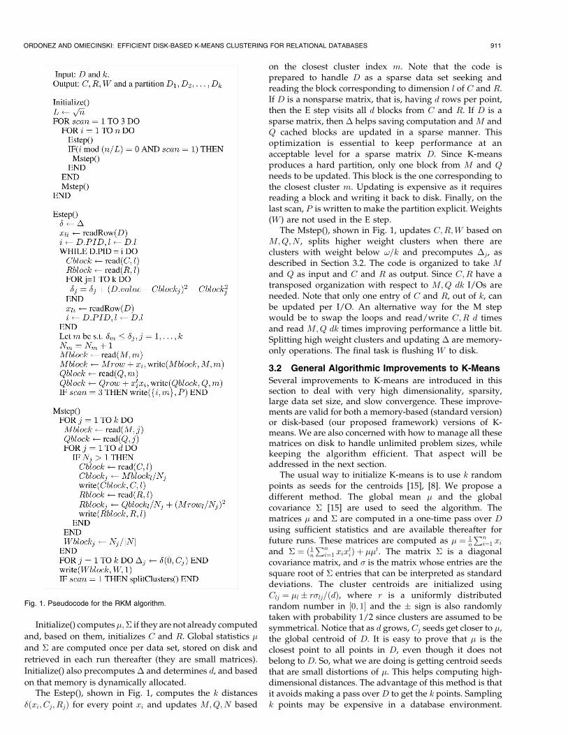
In this section, we present an overview of RKM. Generalalgorithmic improvements are presented in Section 3.2 anda disk organization for matrices is presented in Section 3.3.The RKM pseudocode is given in Fig. 1. This is a high-leveldescription. The algorithm sets initial values of C inInitialize() based on �;� as proposed in Section 3.2. It thenmakes three scans over D. The goal of the first scan is to getgood approximations for centroids Cj by exploiting dataredundancy via frequent M steps and by splitting clusterswhen necessary. The goal of the second and third scan is totune Cj and shrink Rj values, like Standard K-means. Thesecond and third scan are not sensitive to the order of pointsand reduce the sensitivity (if any) to the order of pointsfrom the first scan. The E step is executed n times per scan.The M step is periodically executed L ¼ ffiffiffi

np

times per scan.I/O for D and P is buffered with blocks having b rows. I/Ofor the matrices is also buffered using the correspondingblock as a buffer for matrix rows or columns.

910 IEEE TRANSACTIONS ON KNOWLEDGE AND DATA ENGINEERING, VOL. 16, NO. 8, AUGUST 2004

Initialize() computes �;� if they are not already computed

and, based on them, initializes C and R. Global statistics �

and � are computed once per data set, stored on disk and

retrieved in each run thereafter (they are small matrices).

Initialize() also precomputes� and determines d, and based

on that memory is dynamically allocated.The Estep(), shown in Fig. 1, computes the k distances

�ðxi; Cj; RjÞ for every point xi and updates M;Q;N based

on the closest cluster index m. Note that the code isprepared to handle D as a sparse data set seeking andreading the block corresponding to dimension l of C and R.If D is a nonsparse matrix, that is, having d rows per point,then the E step visits all d blocks from C and R. If D is asparse matrix, then � helps saving computation and M andQ cached blocks are updated in a sparse manner. Thisoptimization is essential to keep performance at anacceptable level for a sparse matrix D. Since K-meansproduces a hard partition, only one block from M and Q

needs to be updated. This block is the one corresponding tothe closest cluster m. Updating is expensive as it requiresreading a block and writing it back to disk. Finally, on thelast scan, P is written to make the partition explicit. Weights(W ) are not used in the E step.

The Mstep(), shown in Fig. 1, updates C;R;W based onM;Q;N , splits higher weight clusters when there areclusters with weight below !=k and precomputes �j, asdescribed in Section 3.2. The code is organized to take M

and Q as input and C and R as output. Since C;R have atransposed organization with respect to M;Q dk I/Os areneeded. Note that only one entry of C and R, out of k, canbe updated per I/O. An alternative way for the M stepwould be to swap the loops and read/write C;R d timesand read M;Q dk times improving performance a little bit.Splitting high weight clusters and updating � are memory-only operations. The final task is flushing W to disk.

3.2 General Algorithmic Improvements to K-Means

Several improvements to K-means are introduced in thissection to deal with very high dimensionality, sparsity,large data set size, and slow convergence. These improve-ments are valid for both a memory-based (standard version)or disk-based (our proposed framework) versions of K-means. We are also concerned with how to manage all thesematrices on disk to handle unlimited problem sizes, whilekeeping the algorithm efficient. That aspect will beaddressed in the next section.

The usual way to initialize K-means is to use k randompoints as seeds for the centroids [15], [8]. We propose adifferent method. The global mean � and the globalcovariance � [15] are used to seed the algorithm. Thematrices � and � are computed in a one-time pass over Dusing sufficient statistics and are available thereafter forfuture runs. These matrices are computed as � ¼ 1

n

Pni¼1 xi

and � ¼ ð1nPn

i¼1 xixtiÞ þ ��t. The matrix � is a diagonal

covariance matrix, and � is the matrix whose entries are thesquare root of � entries that can be interpreted as standarddeviations. The cluster centroids are initialized usingClj ¼ �l � r�lj=ðdÞ, where r is a uniformly distributedrandom number in ½0; 1� and the � sign is also randomlytaken with probability 1/2 since clusters are assumed to besymmetrical. Notice that as d grows, Cj seeds get closer to �,the global centroid of D. It is easy to prove that � is theclosest point to all points in D, even though it does notbelong to D. So, what we are doing is getting centroid seedsthat are small distortions of �. This helps computing high-dimensional distances. The advantage of this method is thatit avoids making a pass over D to get the k points. Samplingk points may be expensive in a database environment.

ORDONEZ AND OMIECINSKI: EFFICIENT DISK-BASED K-MEANS CLUSTERING FOR RELATIONAL DATABASES 911

Fig. 1. Pseudocode for the RKM algorithm.

However, RKM can use that initialization without anychanges to the rest of the algorithm.

When D has many entries equal to zero and d is high,evaluating (1) can be expensive. In typical transactiondatabases, a few dimensions may have nonzero values. So,we precompute a distance from every Cj to the null vector�00. To that purpose, we define the following k-dimensionalvector: �j ¼ dð�00; CjÞ. Then,

dðxi; CjÞ ¼ �j þXd

l¼1;xlj 6¼0

ððxli � CljÞ2 � C2ljÞ:

This precomputation will save time when D has entriesequal to zero (transaction files or high-d data), but will notaffect performance when points in D have no coordinatesequal to zero (low-dimensional numeric files).

Besides speed of convergence, K-means is often criticizedfor finding a suboptimal solution [8], [17], a commonproblem with clustering algorithms [14], [15]. Most of thetimes suboptimality involves several clusters groupedtogether as one while other clusters have almost no pointsor no points at all [8], [17]. So, we propose splitting “heavy”clusters to achieve higher quality results. RKM splits clusterswith higher than average weight and drops those with veryfew points. This process is different from the one proposedin [8], where zero-weight clusters are reseeded to somerandom point that is far from the current centroid. In moredetail, the process is as follows: When a cluster falls below aminimum weight threshold, it is assigned a new centroidcoming from the highest weight cluster. This high weightcluster gets split in two. The two new centroids are randompoints taken within one standard deviation from the heavycluster mean. The reason behind this is that we want to splitclusters without unnecessarily absorbing points that effec-tively belong to other clusters. We introduce a minimumweight threshold ! to control splitting; ! will be an inputparameter for RKM. Let a be the index of the weight of acluster s.t. Wa < !=k. Let b be the index of the weight of thecluster with highest weight. Then, Cb �

ffiffiffiffiffiffiffiffiffiffiffiffiffiffiffiffiffivect½Rj�

pand Cb þffiffiffiffiffiffiffiffiffiffiffiffiffiffiffiffiffi

vect½Rj�p

are the new centroids (the right terms areprecisely one standard deviation). The weight of reseededclusters will be Wb=2. The weight of the old low weightcluster a is ignored and its points are absorbed into otherclusters in future M steps. This process gets repeated untilthere are no more clusters below !=k. Cluster splitting willbe done in the M step.

Sufficient statistics [30], [28], [8], [46], are summaries ofgroups of points (in this case clusters), represented byD1; . . . ; Dk. RKM uses matrices M, N , and Q, where M andQ are d� k and N is k� 1, containing sum of points:Mj ¼

P8xi2Dj

xi, sum of squared points: Qj ¼P

8xi2Djxix

ti,

and number of points per cluster: Nj ¼ jDjj. The outputmatrices C;R;W can be computed from M;Q;N with

Cj ¼ Mj=Nj;

Rj ¼ Qj=Nj �MjMtj=N

2j ;

and

Wj ¼ Nj

�X

J

NJ:

Note that this is a powerful feature since we do not need torefer to D anymore.

Sufficient statistics reduce I/O time by avoiding repeatedscans over the data and by allowing parameter estimationperiodically as transactions are being read. Periodic M stepsare used to accelerate convergence. Remember that clustermembership is determined in the E step and C;R;W areupdated in the M step. By using sufficient statistics, thealgorithm can run the M step at different times whilescanning D. At one extreme, we could have an onlineversion [45], [8] that runs the M step after every point. Thatwould be a bad choice. The algorithm would be slowerbecause of matrix operations and it would also be verysensitive to the order of points because centroids wouldchange after every point is read. At the other extreme, wecould have a version that runs the M step after all n pointsare read. This would reduce it to the standard version ofK-means and no performance improvement would beachieved. However, it must be noted that the standardversion of K-means is not sensitive to the order of pointsand has the potential of reaching a local optimal solution.Therefore, it is desirable to choose a point somewhere in themiddle, but closer to the standard version. That is, runningthe M step as few times as possible. We propose toperiodically execute the M step every n=L points, orequivalently, L times per scan. This accelerates convergencewhen n is large and there is high redundancy in D. To someextent, L resembles number of iterations. In fact, Lwould beequal to the number of iterations if every block of n=Lpoints had the same points. The default value for thenumber of M steps is L ¼

ffiffiffin

p. The reason behind this

number is that the algorithm uses as many points to makeone M step as the number of M steps it executes periteration. The value for L will be fixed and is not considereda running parameter for RKM. Observe that L is indepen-dent from d and k. As n grows, the algorithm will takeadvantage of data set size to converge faster. The E step isexecuted for every point, i.e., n times per scan. The E stepcannot be executed fewer times, unless sampling is done. Ingeneral, RKM will run for three iterations. The first iterationwill obtain a good approximation to C by making frequentM steps and splitting clusters. The second and thirditerations will tune results by making a complete M stepbased on the n data points. They also have the purpose ofreducing sensitivity to the order of points on disk from thefirst iteration. Further iterations can improve quality ofresults by a marginal fraction like the Standard K-meansalgorithm, but for our experiments all measurements aretaken at the end of the third iteration.

3.3 Disk Organization of Matricesand Input Data Set

In this part, we present our proposed disk layout toefficiently manage big clustering problems involving veryhigh dimensionality or a large number of clusters. Ourapproach is different from previous approaches in the sensethat we use disk instead of memory to manage clusteringresults. This may sound counterintuitive given highermemory capabilities and disk performance remaining moreor less constant in modern computer systems [11]. Never-theless, performance is still good giving the ability to


manage problems of unlimited sizes as we shall see.Besides, an algorithm that uses less memory at a reasonablespeed may be preferable to a very efficient algorithm thatuses a lot of memory. In the end, clustering results have tobe stored on disk.

3.3.1 Disk Organization for Input Data Set and

Partition Table

The following discussion is based on the relational model[16], [44]. Our approach assumes the input data set D is in acertain relational form. Instead of assuming we have a plaintable with n d-dimensional rows as most other algorithms,each row contains only the value for one dimension of onepoint when such value is different from zero. This is donefor efficiency reasons when D is a matrix having manyzeroes, which is the case of transaction data. The schema(definition) for D is DðPID; l; valueÞ, where PID is the pointidentifier, l is the dimension subscript, and value is thecorresponding nonzero value. When D has exactly dn rows,we refer to it as a nonsparse matrix; otherwise, (when it hasless rows) D is called a sparse matrix. If D is sparse, it willhave in total td rows, where t is the average of sðxiÞ andsðxiÞ represents the number of nonzero dimensions for xi;the number t can be thought of as average transaction size.In practice, this table may have an index, but for ourimplementation, it will not be required since D is readsequentially. The primary key of D is simply ðPID; lÞ. Thisrepresentation becomes particularly useful when D is asparse matrix, but it is still adequate for any data set.Converting D to our proposed scheme takes time OðdnÞ andis done once per data set. As mentioned in Section 2,K-means produces a hard partition of D into k subsetsD1; D2; . . . ; Dk. Each xi is assigned to one cluster and suchassignment is stored in the table P ðPID; jÞ. So, P containsthe partition of D into k subsets. Each subset Dj can beselected using j to indicate the desired cluster number. Thistable is used for output only and its I/O cost is very lowsince it is written n times during the last scan and each rowis very small. We close this part stressing that disk seeks(positioning the file pointer at a specific disk address insidethe file) are not needed for D and P because they areaccessed sequentially. Also, I/Os are buffered reading agroup of D rows or writing a group of P rows. Thisbuffering capability is provided by the I/O library of theprogramming language. This scenario will be completelydifferent for matrices as we shall see in the followingparagraphs.

3.3.2 Disk Organization for Matrices

Now, we explain how to organize matrices on disk. Thisdisk organization is oriented toward making the RKMimplementation efficient, but it is not strictly relational as itwas the case for D and P . In fact, a pure relational schemewould not work in this case because arrays and subscriptsare needed to manipulate matrices. In any case, it isstraightforward to transform the proposed matrices layoutinto simple relational tables having a primary key and anumber of nonkey columns.

When organizing matrices on disk, there are threepotential alternatives depending on the granularity levelfor I/O:

1. doing one I/O per matrix entry,2. doing one I/O per matrix row or column, or3. doing one I/O for the entire matrix.

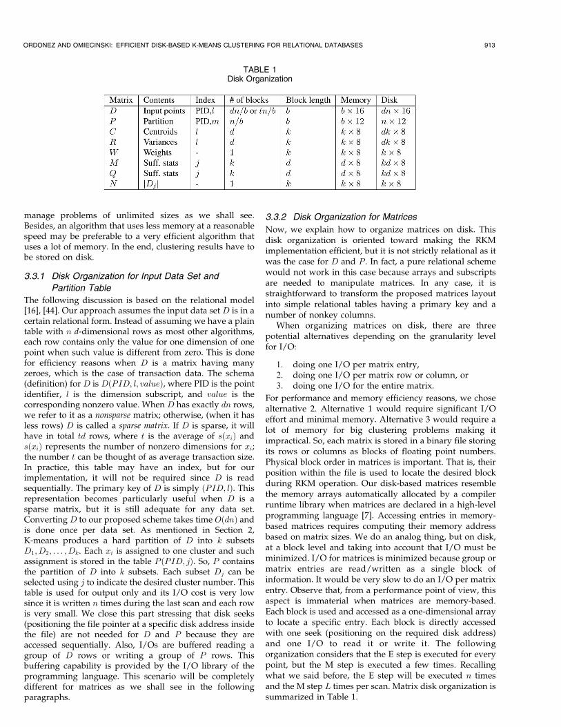
For performance and memory efficiency reasons, we chosealternative 2. Alternative 1 would require significant I/Oeffort and minimal memory. Alternative 3 would require alot of memory for big clustering problems making itimpractical. So, each matrix is stored in a binary file storingits rows or columns as blocks of floating point numbers.Physical block order in matrices is important. That is, theirposition within the file is used to locate the desired blockduring RKM operation. Our disk-based matrices resemblethe memory arrays automatically allocated by a compilerruntime library when matrices are declared in a high-levelprogramming language [7]. Accessing entries in memory-based matrices requires computing their memory addressbased on matrix sizes. We do an analog thing, but on disk,at a block level and taking into account that I/O must beminimized. I/O for matrices is minimized because group ormatrix entries are read/written as a single block ofinformation. It would be very slow to do an I/O per matrixentry. Observe that, from a performance point of view, thisaspect is immaterial when matrices are memory-based.Each block is used and accessed as a one-dimensional arrayto locate a specific entry. Each block is directly accessedwith one seek (positioning on the required disk address)and one I/O to read it or write it. The followingorganization considers that the E step is executed for everypoint, but the M step is executed a few times. Recallingwhat we said before, the E step will be executed n timesand the M step L times per scan. Matrix disk organization issummarized in Table 1.


TABLE 1Disk Organization

In the E step, C and R have to be read for every xi tocompute �ðxi; Cj; RjÞ. Note that W is not needed in the Estep. If D is a sparse matrix, then most dimensions in C;Rwill not be needed to compute �. But, in any case, all kdistances must be computed at each E step. This motivatesstoring C;R with all k values for each cluster as one blockfor each dimension. That is, each row of C and R, asdefined in Section 2 becomes one block. Each block isaccessed using the dimension l as an index. If there are sðxiÞrows for xi, then only sðxiÞ blocks from C and R are read.When sðxiÞ < d this saves significant I/O. As mentionedbefore, we use � to store precomputed distances. Thisauxiliary matrix is small and, therefore, it is kept inmemory. Once the k distances �ðxi; Cj; RjÞ have beencomputed, we have to add xi to the closest cluster throughits sufficient statistics. This means we have to read andwrite only information about one cluster from M and Q.This motivates storing all d dimensions of one cluster as oneblock and using the cluster index j as index. That is, eachcolumn of M and Q, as defined in Section 3.2 becomes oneblock. Let m be the index of the closest cluster. When xi isadded to Mm, we have to read Mm from disk, add xi to it,and then write Mm back to disk. A similar reasoningmotivates organizing Q in the same manner as M. So, onlytwo I/Os are needed to update M and two I/Os are neededto update Q per E step. Note that, in this case, the diskorganization we have for C;R would be inefficient as itwould require d I/Os every time M is updated. Since N isa small matrix, it is kept in memory as one row of k valuesavoiding reading it or writing it. To assign xi to Dm,representing the closest cluster, we just need to write itsPID and m to P in a single I/O.

The M step is expensive in I/O cost since each entry ofevery matrix needs to be accessed and C;R are disk-transposed with respect to M;Q. Matrices M;Q;N have tobe read in order to write C;R;W . But fortunately, the Mstep is executed infrequently and, in general, the size of thematrices is small compared to a large data setD. This makesseeks/reads/writes performance acceptable as we will seein the experimental section. Matrix W can be organized in asimilar manner to N storing the k weights as a single block,but updating it in each M step. By writing C;R;W to disk atevery M step an advantage is gained: The algorithm can bestopped at any time. So, if there is an I/O error whilescanning D or the algorithm is simply interrupted by theuser, the latest results are available on disk. Even further,the exact value of C;R;W could be obtained up to the lastread point by reading M;Q;N , which are updated in everyE step. Due to lack of space, we omit a further discussion onhow to seek, read and write blocks of C;R;W;M;Q and N .

The read/write operations on the data set and allmatrices are summarized in Table 2. The data set D is readin the E step. Since each row corresponds to one dimensiont, I/Os are needed on average per E step ifD is sparse and dotherwise. Also, when cluster membership has beendetermined, P is updated during the 2nd scan. Thisproduces the hard partition. Matrices D and P are notneeded in the M step. As mentioned before, C;R have to beread in the E step. Each access requires one seek and one I/O to read the blocks with k values. For the M step, the story

is quite different since M and Q are transposed. So, 2dk

seeks and I/Os are needed per M step to update C and R,

respectively. Note that this is expensive compared to the E

step. An online version, running the M step after every E

step, would make RKM extremely slow.Key observation. RKM has time complexity OðdknÞ. It

requires OðdkÞ memory operations per E step but only

Oðdþ kÞ I/Os per E step. The M step requires OðdkÞ I/Os,

but it is executed only L ¼ffiffiffin

ptimes per scan. So, M step’s

contribution to disk I/O is insignificant for large n. There-

fore, an entire scan requiresOððdþ kÞnþ dk2Þ ¼ Oððdþ kÞnÞI/Os for large n. This is a key ingredient to get an efficient

algorithm that is disk-based.

3.3.3 Memory and Disk Requirements

This section explains how much memory and how much

disk space is needed by the proposed approach. From

Table 1, it can be seen that memory requirements are

Oðdþ kÞ, which for large clustering problems are much

smaller than OðdkÞ. This latter space complexity is the

minimum requirement for any approach that is memory-

based. I/O for D and P is buffered with blocks having b

rows; this number is independent from d and k. I/O for the

matrices is also buffered using the corresponding block as a

buffer. There is header information not included for space

numbers that includes the matrix name, its number of

blocks, and its number of columns. We ignore the space

required by the header since it is negligible.Disk space requirements are OðdkÞ for matrices OðnÞ for

P and OðdnÞ forD. That is, the algorithm does not introduce

any extra space overhead. We assume points in D are

available in any order as long as all rows (dimensions)

belonging to the same point are contiguous. In practice, this

involves having an index, but note that D is accessed

sequentially; there is no need to search a key or make

random access. On the other hand, matrix organization is

fixed throughout the algorithm execution. Then, each block

can either be located through an index or through a direct

disk address computation. In our case, we directly compute

disk addresses based on matrix size and desired dimension

l or cluster number j. Storage for D assumes PID and

dimension are four byte integers and dimension value a

double precision (eight bytes). Storage for all matrices is

based on double precision variables. Disk usage in bytes is

summarized in Table 1.


TABLE 2Read/Write Usage of Matrices

3.4 Examples

We show two examples of potential input data sets andtheir corresponding clustering output in Fig. 2. Recall thateach block of C represents one dimension, each block hask ¼ 2 values, and it is read/written in a single I/O. Blocksare identified and located (via a disk seek) by dimensionindex l. As mentioned before, matrix block order isimportant; in fact, the examples show C exactly as it isphysically stored on disk. W only has one block containingthe k cluster weights. Due to lack of space, we do not showR or sufficient statistics M;Q;N , but they follow the layoutdefined in Section 3.3.

The first example represents a data set D having d ¼ 3and n ¼ 4. This data set is a nonsparse matrix. In this case,there are two clusters clearly represented by the repeatedrows. The cluster centroids and weights appear to the right.It can be the case that some dimensions are not present asrows when their value is zero. That is the case with the rightdata set, which is sparse.

The second example shows a hypothetical transactiontable D containing items treated as a sparse binary matrix.For this data set, d ¼ 4 and n ¼ 5. Those items that are notpresent in a transaction do not appear as rows, as it happensin a typical database environment. The d items are treatedas binary dimensions. When the item is present thedimension value is one. Otherwise, a value of zero isassumed. However, this value could stand for some metriclike item price or item quantity if clustering was desired onsuch characteristics. Clusters appear on the right just likethe first example; first the centroids and then the weights.

4 EXPERIMENTAL EVALUATION

This section presents an extensive experimental evaluation.RKM is compared against the Standard K-means algorithm

[17], [15] and the well-known Scalable K-means algorithm[8]. We implemented the improved Scalable K-meansalgorithm proposed in [17]. Both Standard K-means andScalable K-means use memory to manipulate C;R;W andM;Q;N and access disk only to read D or write P . On theother hand, RKM uses disk all the time keeping one block ofeach matrix in memory at any given moment. All experi-ments were performed on a Personal Computer running at800 MHz with 64 MB of memory and a 40 GB hard disk. Allalgorithms were implemented in the C++ language. Nooptimizations such as parallel processing, multithreading,caching files, or compression were used in the followingtests.

There are three sections discussing experiments with realdata sets, synthetic numeric data sets, and synthetictransaction data sets, respectively. Although there is nouniversal agreement, we consider 20 dimensions or less lowdimensionality, from 30 to 100 high dimensionality, and1,000 and beyond very high dimensionality. In general, inorder to use K-means it is necessary to normalize ortransform the input data set D to have dimensions withsimilar scales since K-means assumes spherical Gaussians[39]. All data sets were transformed to have zero mean andunit variance before using the algorithms using a z-scoretransformation [28].

The main input parameter was k, the desired number ofclusters. I/O for D and P was buffered using b ¼ 100 rowsfor RKM. To stop Scalable K-means and Standard K-means,we used a tolerance threshold of 0:001 for the quantizationerror to get acceptable results. A smaller threshold wouldonly slow the algorithms and it would marginally improvethe quality of solutions. Buffer size for Scalable K-meanswas set at 1 percent of n, which was the best settingaccording to the experiments reported in [8] and [17]. For


Fig. 2. Examples of a multidimensional numeric data set and a transaction data set.

RKM, the default weight threshold was ! ¼ 0:2 to reseedclusters. For Scalable K-means, zero-weight clusters werereseeded to the furthest neighbor as explained in [8], [17].Cluster centroids were not reseeded for Standard K-meansunder any circumstance.

The three algorithms used Euclidean distance and werecompared with the quantization error defined in (2)(average distance from each data point to the centroid ofthe cluster containing the point). For RKM, the global mean� and the global variance � were used to initialize Cj, asexplained in Section 3.2. For Scalable K-means andStandard K-means, k random points were used as seedsfor Cj, which is the most common way to seed K-means asexplained in Section 2.

4.1 Real Data Sets

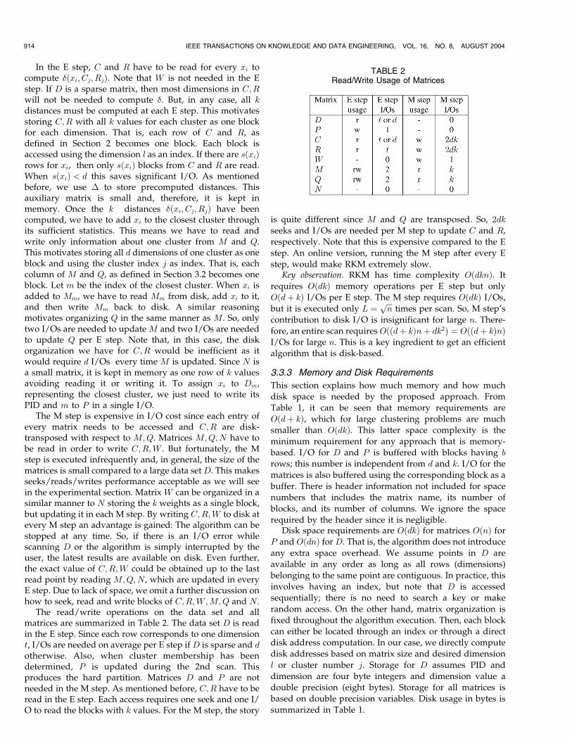
In general with real data it is not possible to find the globaloptimal clustering solution. Therefore, the only acceptableway to compare the algorithms is by analyzing thequantization error; the lower the better. It is customary torun K-means several times to find a good clusteringsolution. Table 3 contains the quantization error andelapsed time to find the best solution out of 10 runs withseveral real data sets with two different values of k for eachof them.

This is a short description of each data set. TheAstronomy data set sizes were n ¼ 36; 889 and d ¼ 4; thisdata set contained information about stars and wasobtained from the California Institute of Technology. TheMedical data set sizes were n ¼ 655 and d ¼ 13; this data setcontained information about patients being treated for heartdisease and was obtained from the Emory UniversityHospital. The Internet data set had n ¼ 10; 105 points withd ¼ 72. This data set contained log information from usersat a Web site and was taken from the UCI MachineLearning repository; it had many zeroes. The US Censusdata set had n ¼ 8; 000 points with d ¼ 68 sampled from theUS census data set available from the UCI MachineLearning repository; this data set had many zeroes. TheVotes data set contained categorical columns about a sampleof voters in 1984 and was obtained from the UCI MachineLearning Repository. Dimensions were converted to binary.It had n ¼ 435; d ¼ 17. This was a small data set with manyzeroes.

In seven instances, RKM found the best solution. In twoproblem instances (Astronomy), Standard K-means foundthe best solution, but the solution found by RKM was veryclose. RKM and Standard K-means were tied in oneinstance. In general, Scalable K-means came in third place.Even though a lower quantization error means a betterclustering solution, there was not a significant difference inthe quality of the solutions found by the three algorithms.For small data sets, the three algorithms had similarperformance. For low-dimensional large data sets (Astron-omy), Scalable K-means was the fastest, with RKM comingsecond being about twice as slow. For high-dimensionallarge data sets (USCensus and Internet), RKM and ScalableK-means had similar performance, and Standard K-meanswas about an order of magnitude worse. RKM tookadvantage of the abundance of zeroes for these high-dimensional data sets.

4.2 Numeric Synthetic Data Sets

The numeric synthetic data generator we used allowed usto generate clusters having a multidimensional Gaussian(normal) distribution. The generator allows specifying d, k,n, the scale for dimensions, the cluster radiuses Rj, and anoise level �. In general, we kept dimensions in the ½0� 100�range and cluster radiuses at 10, so that they could overlapand at the same time not be perfectly separated. Note that,since clusters follow a normal distribution, they containpoints that are up to �3� from � [15], [28]. The defaultswere n ¼ 10; 000; d ¼ 10, k ¼ 10, and � ¼ 1 percent.

Noise, dimensionality, and a high number make cluster-ing a more difficult problem [2], [4], [43], [8]. The followingexperiments analyze the algorithm behavior under eachaspect. The next set of experiments is not complete as we donot show what happens when we vary combinations ofthese parameters, but we chose values that are common in atypical data mining environment.

4.2.1 Quality of Results

Accuracy is the main quality concern for clusters. Aconfusion matrix [2], [15] is a common tool to evaluateclustering accuracy when clusters are known. But, thatwould allow us to show only a few results. In our case, onecluster is considered accurate if there is no more than � errorin its centroid and weight. This is computed as follows: Letcj; wj be the correct mean and weight, respectively, (as


TABLE 3Quality of Results and Performance with Real Data Sets

given by the data generator) of cluster j having estimatedCj;Wj values by the clustering algorithm, and let � be theestimation error. Then, cluster j is considered accurate ifð1=dÞ

Pdl¼1 jclj � Cljj=jcljj � � and jwj �Wjj=wj � �. For the

experiments below, we set � ¼ 0:1. That is, we will considera cluster to be correct if it its mean and weight differ by nomore than 10 percent from the generated cluster. Theprocess to check clusters for accuracy is as follows: Clusterseeds are generated in a random order and then clusteringresults may also appear in any order. So, there are manypermutations in which clusters may correspond to eachother (k!). To check clusters, we build a list of pairs(estimated, generated) clusters. Each estimated cluster ismatched (by distance) with the closest synthetic cluster andit is eliminated from further consideration. For eachmatched cluster, we compute its accuracy error accordingto its weight and centroid. If both are below �, thediscovered cluster will be considered accurate.

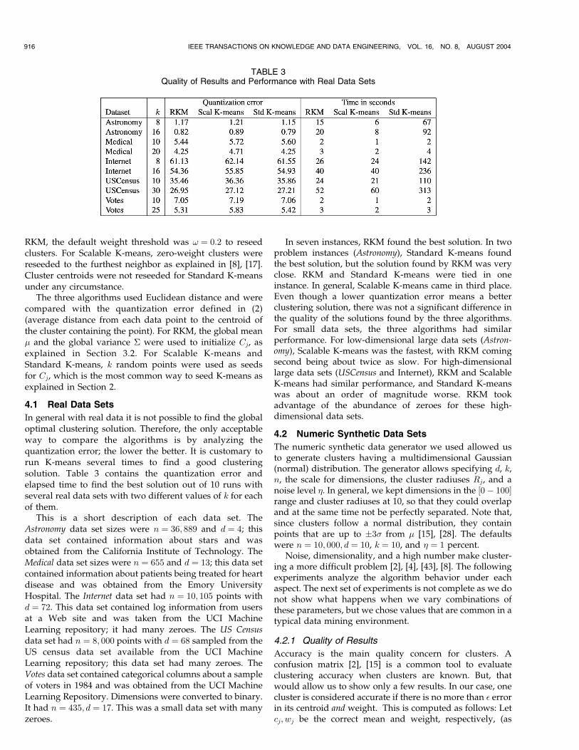
In graphs shown in Fig. 3, we evaluate quality of resultsunder a variety or conditions. All the algorithms were runwith kþ 1 clusters in order to separate noise as a potentialcluster. The graphs in Fig. 3 show the average percentage ofaccurate clusters in 10 runs. They represent what the usermight expect from running the algorithm once. Whenanalyzing the average run in more detail, we have thefollowing: The first graph shows what happens when noiseis gradually incremented. It can be seen that RKM outper-forms the other two algorithms by a wide margin. In thesecond graph, we show what happens when dimensionalitygrows. RKM performs best, Scalable K-means comes secondand Standard K-means comes last. There is no significantdifference. The third graph shows what happens when thedata set contains an increasing number of clusters. SinceK-means is not hierarchical, it has trouble identifying low-weight clusters. RKM again finds a higher percentage ofaccurate clusters than their rivals; getting more than80 percent of clusters right when k ¼ 50. Due to lack ofspace, we do not show graphs with the best run out of10 runs; results are similar, but percentages are higher forall algorithms.

Table 4 shows the average quantization error for 10 runsof each algorithm with n ¼ 10k. This table corresponds tosome instances graphed in Fig. 3. This table gives morespecific evidence about the quality of solutions found byeach algorithm on well-separated clusters. RKM finds the

best solution in all instances. Scalable K-means finds bettersolutions than Standard K-means at the lower noise levels.At higher noise, Scalable K-means is slightly worse thanStandard K-means. We can conclude that quality-wise RKMperforms better than Scalable K-means and StandardK-means, and Scalable K-means and Standard K-meansfind solutions of similar quality on well separated clusterswith a low level of noise.

4.2.2 Performance

This section analyzes performance. We excluded the time totransform D into the proposed relational scheme. Thatprocess is executed once per data set and takes time OðdnÞas explained in Sections 3.2 and 3.3.

In Fig. 4, we evaluate how much performance is lost byhaving a disk-based implementation. The default sizes weren ¼ 100k, d ¼ 10, and k ¼ 10. In the memory-based im-plementation, the algorithm is identical but it does not usedisk at all to manage matrices. In the disk-based imple-mentation, we use the proposed disk organization and diskaccess optimizations. In the memory-based implementa-tion, we use dynamic matrices based on pointers anddynamic memory allocation. These comparisons try toanswer the question of how much speed we are losing inperformance by using disk instead of memory. To oursurprise, it was not much and, in fact, for higherdimensionality the disk-based implementation was better.A close inspection revealed I/O cost is amortized as dgrows, while memory access remains constant. Anotherreason is that our memory-based version uses dynamicmemory allocation for matrices. This introduces some


Fig. 3. Quality of results with synthetic data sets: average percentage of accurate clusters.

TABLE 4Quality of Results with Synthetic Data Sets:

Average Quantization Error

overhead. A memory-based version with static arrayswould be slightly faster. Nevertheless, that option isdiscarded since it is not practical in a real-world scenario.So, this is telling us it would not be worth it to try tooptimize the algorithm by caching the most frequentlyaccessed blocks of the matrices. There would be aperformance gain, but it would not be significant andmemory management overhead could even make it slower.

In Fig. 5, we compare RKM performance againstStandard K-means and Scalable K-means. We used datasets having the following defaults: d ¼ 10, k ¼ 10, andn ¼ 10k. Clearly, times scale linearly for RKM. Scalable K-means is the fastest, RKM comes second, and Standard K-means comes last. Observe that, in order for K-means tohave similar performance to RKM, it would need toconverge to an acceptable solution in no more than threeiterations, which is unlikely in practice.

4.3 Very High-Dimensional Synthetic Data Sets

We used synthetic transaction data sets to evaluate RKMagainst very high-d data sets. The IBM synthetic datagenerator has seven parameters to generate transactionscontaining items to test association rule algorithms [5], [6]. Ingeneral,weonlyvariedn (numberof transactions, calledDbythe generator), t (average transaction size, called T by thegenerator), averagepattern length (about 1/2 of T and called Iby the generator), and used defaults for the rest, unlessspecified otherwise. The number of items d (called nitems bythe generator) was set to 1,000 or 10,000. The defaults arenumber of patterns npatterns ¼ 1; 000, average rule con-fidence conf ¼ 0:75, and item correlation corr ¼ 0:25. Trans-action files are named after the parameters with which they

were created. The standard way [6] is to use T , I, and D tolabel files since those are the three most common parametersto change.

4.3.1 Performance

In Fig. 6, we show performance graphs to cluster sparsetransaction files containing transactions. It was not possibleto run Standard K-means or Scalable K-means given the bigmemory requirements and running time. The chosen testfile was T10I5D100k; which is one of the most common filesused in the literature [6], [23]. The number of transactionswas 100k by default, the average transaction size was 10,and the average pattern length is 5. There are some basicdifferences between these data sets and the multidimen-sional data sets shown before: they are binary, dimension-ality is very high, noise content is low, and transactions arevery sparse vectors (with 10 items present out of 1,000 or10,000). In each case, we plot the times to cluster with d ¼1; 000 and d ¼ 10; 000. We can see that performance isminimally affected by dimensionality because the averagetransaction size remains constant.

5 RELATED WORK

BIRCH [46] is an important precursor of scalable clusteringalgorithms used in a database environment. It is looselybased on K-means and keeps a similar set of sufficientstatistics as ours (sums of points and sums of squaredpoints). However, it is hierarchical, memory-based, and ithas been shown that it does not work well with high-dimensional data or a high level of noise [24]. Improving


Fig. 4. Performance: comparing disk versus memory implementations.

Fig. 5. Performance: time cluster numeric data sets. Defaults: n ¼ 10k, d� 10, and k ¼ 10.

K-means to find higher quality solutions has been investi-gated before. The idea of splitting and merging clustersbased on the EM algorithm is presented in [43]. The maindifferences with [43] are that we do not merge clusters, oursplitting criterion is simpler (since we do not computedistances between two distributions), several clusters maybe divided at the same time in a single M step, and we splithigh weight clusters that are sparser. Their experimentsshow high-quality solutions are found, but computationalcost is increased five times. Moving bad centroids to betterlocations in K-means is presented in [19]. This approach isalso different from ours. Only one bad cluster is discardedat the end of an iteration, while we may split severalclusters in one M step, the splitting criterion is morecomplex and the computation cost is higher. A memory-based K-means algorithm to cluster binary data streamswas introduced in [34]; this algorithm is faster and moreefficient than RKM, but it is only suitable for sparse binarydata. The well-known Scalable K-means algorithm isintroduced in [8]. This is a memory-based algorithm, alsobased on sufficient statistics, that makes compression in twophases for dense and quasi-dense regions. It only requiresone scan over the data, but it makes heavier CPU use and itrequires careful tuning of running parameters (buffer size,compression ratio). The authors use it to build severalmodels concurrently incurring a high overhead, but havingthe ability to automatically pick the highest quality model.They propose reseeding empty clusters to low probabilityclusters. No splitting is done; basically, a bad cluster ismoved to a far location where it has a higher chance ofgetting points. An important improvement of ScalableK-means was introduced in [17]. The authors simplifybuffer management and make extensive comparisons withseveral versions of K-means. One of their findings is thatK-means with sampling is inaccurate. They also show thatScalable K-means is slightly faster than Standard K-meansand, in fact, in some cases, it turns out to be slower giventhe overhead to perform the two-phase compression. Theyalso show that the quality of solutions for StandardK-means and Scalable K-means is about the same on highdimensional data. They show their improved version ofScalable K-means is faster than Standard K-means and findssolutions of similar quality. These facts motivated us tocompare against Standard K-means and the improvedversion of Scalable K-means. A related approach to

integrate a clustering algorithm with a relational DBMS ispresented in [35], where SQLEM is introduced. SQLEMrepresents the EM clustering algorithm programmed inSQL and, therefore, executing on top of the query optimizerwithout directly accessing the file management system.RKM represents the counterpart of SQLEM, directlyaccessing the file management system, and overriding thequery optimizer. This article presented a prototype forsequential processing, but more research is needed to get atighter integration with a parallel DBMS. Many aspectsabout RKM can also be applied to the EM clusteringalgorithm. That topic is also subject of future research.

6 CONCLUSIONS

This article presented a disk-based K-means clusteringalgorithm, called RKM, suitable to be programmed insidea relational DBMS. RKM is designed to manage bigclustering problem sizes. We proposed a series of algorith-mic improvements as well as a disk organization scheme forthe data set and matrices. Its main algorithmic improve-ments include sparse matrix manipulation, periodicM steps,mean-based initialization, and cluster splitting. The algo-rithm only requires three scans over the data to cluster asparse data set. The algorithm does not use sampling. Weproposed a disk organization for the input data set and thematrices. We recommend organizing the input data set D ina relational form with one row per dimension value for eachpoint. In this manner, we can easily manage sparse data setsandmake dimension an explicit index for matrices. Our diskorganization for matrices is based on the assumption that theE step is executed for every point and the M step is executeda few times per iteration. We recommend organizing themeansmatrixC and variancesmatrixRwith d blocks havingk values each. In contrast, we recommend organizingM andQ with k blocks having d values each. N and W can beupdated inmemory because they are small, but writingW inevery M step. This allows results to be available at any timeshould the algorithm be interrupted. Experimental evalua-tion shows RKM can obtain solutions of comparable qualityto Standard K-means and Scalable K-means on a variety ofreal and synthetic data sets.We also included experiments tojustify RKM’s capability to cluster high-dimensional trans-action files. Performance is linear in the number of points,dimensionality, desired number of clusters, and transaction


Fig. 6. Performance time cluster transaction data sets. Defaults: n ¼ 100k, k ¼ 10, and T ¼ 10.

size. Performance is minimally affected by dimensionality

when transaction size remains constant. RKM has no

practical memory limitations.

6.1 Future Work

Since RKM can cluster binary data, we want to investigate

how good it is to cluster categorical data. Caching several

rows of the matrices does not seem a promising research

direction given our experiments, but there may be

optimizations we cannot foresee. We would like to use

our algorithm as a foundation to build more complex data

mining programs inside relational Database Management

Systems. We would like to explore other data mining

techniques that use memory intensively and modify them

to work on disk keeping performance at an acceptable level.

ACKNOWLEDGMENTS

The authors wish to thank the reviewers for their

comments. The first author specially thanks the reviewer

who suggested using quantization error as the basic quality

criterion and the reviewer who suggested performing

experiments with real data.

REFERENCES

[1] C. Aggarwal, C. Procopiuc, J. Wolf, P. Yu, and J. Park, “FastAlgorithms for Projected Clustering,” Proc. ACM SIGMOD Conf.,1999.

[2] C. Aggarwal and P. Yu, “Finding Generalized Projected Clustersin High Dimensional Spaces,” Proc. ACM SIGMOD Conf., 2000.

[3] C. Aggarwal and P. Yu, “Outlier Detection for High DimensionalData,” Proc. ACM SIGMOD Conf., 2001.

[4] R. Agrawal, J. Gehrke, D. Gunopolos, and P. Raghavan, “Auto-matic Subspace Clustering of High Dimensional Data for DataMining Applications,” Proc. ACM SIGMOD Conf., 1998.

[5] R. Agrawal, T. Imielinski, and A. Swami, “Mining AssociationRules between Sets of Items in Large Databases,” Proc. ACMSIGMOD Conf., pp. 207-216, 1993.

[6] R. Agrawal and R. Srikant, “Fast Algorithms for MiningAssociation Rules in Large Databases,” Proc. Very Large Data BaseConf., 1994.

[7] A. Aho, R. Sethi, and J.D. Ullman, Compilers: Principles, Techniquesand Tools. pp. 200-250, Addison-Wesley, 1986.

[8] P. Bradley, U. Fayyad, and C. Reina, “Scaling ClusteringAlgorithms to Large Databases,” Proc. ACM KDD Conf., 1998.

[9] P. Bradley, U. Fayyad, and C. Reina, “Scaling EM Clustering toLarge Databases,” technical report, Microsoft Research, 1999.

[10] M. Breunig, H.P. Kriegel, P. Kroger, and J. Sander, “Data Bubbles:Quality Preserving Performance Boosting for Hierarchical Clus-tering,” Proc. ACM SIGMOD Conf., 2001.

[11] S. Chaudhuri and G. Weikum, “Rethinking Database SystemArchitecture: Towards a Self-Tuning RISC-Style Database Sys-tem,” Proc. Very Large Data Base Conf., 2000.

[12] J. Clear, D. Dunn, B. Harvey, M.L. Heytens, and P. Lohman,“Nonstop SQL/MX Primitives for Knowledge Discovery,” Proc.ACM KDD Conf., 1999.

[13] A.P. Dempster, N.M. Laird, and D. Rubin, “Maximum LikelihoodEstimation from Incomplete Data via the EM Algorithm,” J. RoyalStatistical Soc., vol. 39, no. 1, pp. 1-38, 1977.

[14] R. Dubes and A.K. Jain, Clustering Methodologies in ExploratoryData Analysis. pp. 10-35, New York: Academic Press, 1980.

[15] R. Duda and P. Hart, Pattern Classification and Scene Analysis.pp. 10-45, J. Wiley and Sons, 1973.

[16] R. Elmasri and S.B. Navathe, Fundamentals of Database Systems,third ed. pp. 841-871, Addison-Wesley, 2000.

[17] F. Fanstrom, J. Lewis, and C. Elkan, “Scalability for ClusteringAlgorithms Revisited,” SIGKDD Explorations, vol. 2, no. 1, pp. 51-57, June 2000.

[18] U. Fayyad, G. Piatetsky-Shapiro, and P. Smyth, “The Kdd Processfor Extracting Useful Knowledge from Volumes of Data,” Comm.ACM, vol. 39, no. 11, pp. 27-34, Nov. 1996.

[19] B. Fritzke, “The LBG-U Method for Vector Quantization—AnImprovement over LBG Inspired from Neural Networks,” NeuralProcessing Letters, vol. 5, no. 1, pp. 35-45, 1997.

[20] V. Ganti, J. Gehrke, and R. Ramakrishnan, “Cactus-ClusteringCategorical Data Using Summaries,” Proc. ACM KDD Conf., 1999.

[21] S. Guha, R. Rastogi, and K. Shim, “Cure: An Efficient ClusteringAlgorithm for Large Databases,” Proc. SIGMOD Conf., 1998.

[22] S. Guha, R. Rastogi, and K. Shim, “Rock: A Robust ClusteringAlgorithm for Categorical Attributes,” Proc. Int’l Conf. Data Eng.,1999.

[23] J. Han, J. Pei, and Y. Yun, “Mining Frequent Patterns withoutCandidate Generation,” Proc. ACM SIGMOD Conf., 2000.

[24] A. Hinneburg and D. Keim, “Optimal Grid-Clustering: TowardsBreaking the Curse of Dimensionality,” Proc. Very Large Data BaseConf., 1999.

[25] Z. Huang, “Extensions to the k-Means Algorithm for ClusteringLarge Data Sets with Categorical Values,” Data Mining andKnowledge Discovery, vol. 2, no. 3, 1998.

[26] M. Jordan and R. Jacobs, “Hierarchical Mixtures of Experts andthe EM Algorithm,” Neural Computation, vol. 6, no. 2, 1994.

[27] J.B. MacQueen, “Some Methods for Classification and Analysis ofMultivariate Observations,” Proc. Fifth Berkeley Symp. Math.Statistics and Probability, 1967.

[28] A. Mood, F. Graybill, and D. Boes, Introduction to the Theory ofStatistics. pp. 299-320, New York: McGraw Hill, 1974.

[29] A. Nanopoulos, Y. Theodoridis, and Y. Manolopoulos, “C2p:Clustering Based on Closest Pairs,” Proc. Very Large Data BasesConf., 2001.

[30] R. Neal, G. Hinton, “A View of the EM Algorithm that JustifiesIncremental, Sparse and Other Variants,” technical report, Dept.of Statistics, Univ. of Toronto, 1993.

[31] A. Netz, S. Chaudhuri, U. Fayyad, and J. Berhardt, “IntegratingData Mining with SQL Databases: Ole Db for Data Mining,” Proc.IEEE Int’l Conf. Data Eng., 2001.

[32] M. Ng, “K-means Type Algorithms on Distributed MemoryComputers,” Int’l J. High Speed Computing, vol. 11, no. 2, 2000.

[33] R. Ng and J. Han, “Efficient and Effective Clustering Method forSpatial Data Mining,” Proc. Very Large Data Bases Conf., 1994.

[34] C. Ordonez, “Clustering Binary Data Streams with K-means,”Proc. ACM DKMD Workshop, 2003.

[35] C. Ordonez and P. Cereghini, “SQLEM: Fast Clustering in SQLUsing the EM Algorithm,” Proc. ACM SIGMOD Conf., 2000.

[36] C. Ordonez and E. Omiecinski, “FREM: Fast and Robust EMClustering for Large Data Sets,” Proc. ACM Conf. Information andKnowledge Management, 2002.

[37] D. Pelleg and A. Moore, “Accelerating Exact K-means Algorithmswith Geometric Reasoning,” Proc. Knowledge Discovery and DataMining Conf., 1999.

[38] R.A. Redner and H.F. Walker, “Mixture Densities, MaximumLikelihood, and the EM Algorithm,“ SIAM Rev., vol. 26, pp. 195-239, 1984.

[39] S. Roweis and Z. Ghahramani, “A Unifying Review of LinearGaussian Models,” Neural Computation, 1999.

[40] S. Sarawagi, S. Thomas, and R. Agrawal, “Integrating Mining withRelational Databases: Alternatives and Implications,” Proc. ACMSIGMOD Conf., 1998.

[41] D. Scott, Multivariate Density Estimation, pp. 10-130. New York:J. Wiley and Sons, 1992.

[42] M. Seigel, E. Sciore, and S. Salveter, Knowledge Discovery inDatabases. AAAI Press/The Mit Press, 1991.

[43] N. Ueda, R. Nakano, Z. Ghahramani, and G. Hinton, “SMEMAlgorithm for Mixture Models,” Neural Information ProcessingSystems, 1998.

[44] J.D. Ullman, Principles of Database and Knowledge-Base Systems,vol. 1. Rockville, Md: Computer Science Press, 1988.

[45] L. Xu and M. Jordan, “On Convergence Properties of the EMAlgorithm for Gaussian Mixtures,” Neural Computation, vol. 7,1995.

[46] T. Zhang, R. Ramakrishnan, and M. Livny, “Birch: An EfficientData Clustering Method for Very Large Databases,” Proc. ACMSIGMOD Conf., 1996.


Carlos Ordonez received the BS degree inapplied mathematics and the MS degree incomputer science both from the UNAM Univer-sity, Mexico, in 1992 and 1996, respectively. Hereceived the PhD degree in computer sciencefrom the Georgia Institute of Technology, Atlan-ta, in 2000. Dr. Ordonez currently works forTeradata, a division of NCR Corporation, doingresearch and consulting on Data Mining tech-nology. He has published more than 10 research

articles and holds three patents related to data mining.

Edward Omiecinski received the PhD degreefrom Northwestern University in 1984. He iscurrently an associate professor at the GeorgiaInstitute of Technology in the College of Com-puting. He has published more than 60 papers ininternational journals and conferences dealingwith database systems and data mining. Hisresearch has been funded by the US NationalScience Foundation, DARPA, and NLM. He is amember of the ACM.

. For more information on this or any other computing topic,please visit our Digital Library at www.computer.org/publications/dlib.


Documents

IEEE TRANSACTIONS ON KNOWLEDGE AND DATA …pramanik/teaching/courses/cse880/14f/seminars/... · Abstract—K-means is one of the most popular clustering algorithms. This article introduces